This work is distributed as a Discussion Paper by the

STANFORD INSTITUTE FOR ECONOMIC POLICY RESEARCH

SIEPR Discussion Paper No. 15-­‐009 Trade Intermediation, Financial Frictions, and the Gains from

Trade

By

Jackie M.L. Chan

Stanford Institute for Economic Policy Research Stanford University Stanford, CA 94305 (650) 725-­‐1874

The Stanford Institute for Economic Policy Research at Stanford University supports

research bearing on economic and public policy issues. The SIEPR Discussion Paper Series reports on research and policy analysis conducted by researchers affiliated with the

Institute. Working papers in this series reflect the views of the authors and not necessarily those of the Stanford Institute for Economic Policy Research or Stanford University

Trade Intermediation, Financial Frictions, and

the Gains from Trade

Jackie M.L. Chan∗

March 25, 2015

JOB MARKET PAPER

Most current version available at: http://stanford.edu/~jmlchan/

Abstract

This paper develops a heterogeneous firm model of international trade with trade in-

termediation and financial frictions. Indirect exporting through intermediaries entails lower

fixed costs but larger variable costs, and thus intermediaries alleviate financial frictions which

magnify the fixed cost of exporting. The model finds strong empirical support in firm-level

data on indirect exports for 118 countries as well as country-level data on entrepot trade

through Hong Kong for over 50 countries. Financially more constrained exporting firms and

financially less developed countries are more likely to use trade intermediaries. Both of these

effects are stronger in financially more vulnerable industries. Calibrating a two-country ver-

sion of the model in general equilibrium for China and US reveals important gains from

trade intermediation. When indirect exporting is eliminated from China, welfare, exports,

and the share of exporting firms fall by 0.24%, 18%, and 59% respectively.

JEL classification codes: F10, F14, F36, G20

Keywords: intermediaries, indirect exports, financial constraints, gains from trade, Hong

Kong.

∗I am deeply indebted to Kalina Manova, Kyle Bagwell, and Renee Bowen for their invaluable advice. Ialso want to thank Dave Donaldson, Pete Klenow, Robert Hall, Seunghoon Lee, and Stephen Terry. Supportfrom the Leonard W. Ely and Shirley R. Ely Graduate Student Fund Fellowship of the Stanford Institute forEconomic Policy Research (SIEPR) is gratefully acknowledged. Correspondence: Jackie M.L. Chan, Departmentof Economics, Stanford University, 579 Serra Mall, Stanford, CA 94305, jmlchan@stanford.edu.

1

1 Introduction

Intermediaries facilitate transactions between different parties in many markets. In interna-

tional trade, third-party intermediaries allow firms to sell goods abroad without having to

directly export to the destinations themselves. These indirect trade flows are observed through

trade intermediaries like retailers, wholesalers, or trading companies that match buyers and

sellers across borders. Despite the reduction in barriers to trade, exporting to foreign countries

remains a costly endeavor. Although potentially less profitable, indirect exporting is a cheaper

alternative for producers that cannot afford the large upfront costs of selling abroad. This pa-

per examines the determinants of intermediary trade, with a focus on financial frictions, and

quantifies the effect of trade intermediation on the gains from trade.

Trade intermediaries may be located in domestic or foreign markets. It is estimated that

10 to 20% of exports are sold through domestic intermediaries in countries like the US, Italy,

China, and France (Bernard et al. 2010, Bernard et al. 2013, Ahn et al. 2011, Crozet et al.

2013). According to the World Bank Enterprise Surveys, the average share of exports sold

indirectly through a domestic third-party across many developing countries is substantial at

21%.1 Indirect exports may also flow through intermediaries in a foreign country before reaching

their final destination. This type of indirect exports is commonly referred to as “re-exports”,

or the exports of foreign goods. Globally, the share of re-export trade has been estimated to

be around 15% (Andriamananjara et al. 2004). Re-export trade activity is especially large for

entrepots or trading ports like Hong Kong. Trading companies in Hong Kong such as Li &

Fung Limited have a network of manufacturers in Asia and they assist these firms in finding

customers for their products. Trade intermediation in Hong Kong is extremely large: In 2010,

the value of re-exports through Hong Kong was almost $400 billion USD, while the ratio of

re-exports to gross exports from Hong Kong was 96%.

I develop a heterogeneous firm model of international trade with trade intermediation and

financial frictions. Firms have access to two export modes: direct and indirect. By indirectly

exporting through an intermediary, firms save on fixed costs (e.g., marketing, distribution, prod-

uct design), but face higher variable costs due to additional re-routing transportation costs and

a fee for the intermediary’s services. This trade-off implies that the most productive firms with

high revenue export directly while less productive firms sell indirectly. Besides productivity,

financial market frictions also importantly affect the sorting of firms into export modes. Specif-

ically, the (fixed) cost of exporting requires outside financing, and is therefore magnified by

financial frictions which raise the cost of capital. This can incentivize firms to export indirectly

as the relatively cheaper alternative. The theory thus predicts that financially constrained firms

are more likely to be indirect exporters. Correspondingly, in the aggregate, financially devel-

oped countries with lower costs of credit for all firms have a smaller fraction of exports that are

indirectly sold. Furthermore, these effects are more pronounced in financially more vulnerable

sectors.

1On the import side, Chilean wholesalers accounted for 35% of imports from Argentina (Blum et al. 2010).

2

I test the firm-level implications of the model using the World Bank Enterprise Surveys,

a firm-level dataset covering 118 developing countries. The data provide information on firms

direct exports and indirect exports through domestic intermediaries, as well as a measure of

their financial frictions. The latter is captured by asking whether access to financing, like

availability and cost, is an obstacle to the firm’s operations.2 The results confirm that firms

with greater difficulty in accessing finance are more likely to be indirect exporters. Moreover,

exploiting variation in sector financial vulnerability which is exogenous from the perspective

of individual firms, I find that the interaction effect of financial constraints on the likelihood

of indirect exporting is indeed stronger in sectors with higher external finance dependence and

lower asset tangibility. These two measures capture, respectively, firms’ demand for outside

financing within a given industry and the availability of collateralizable assets to raise financial

capital (Rajan and Zingales 1998, Braun 2003).

At the aggregate level, I examine the bilateral share of indirect exports in total exports

for each pair of countries. Systematic data on this aggregate indirect export share is available

only for re-exports by foreign intermediaries in the entrepot of Hong Kong. This data of

intermediary trade is unique in identifying both origin and destination countries. Using a

sample of 56 exporters, 85 importers, and 25 industries, I estimate a fractional probit model

following the method of Papke and Wooldridge (2008), where the regressors are the exporter’s

financial development and its interactions with sector financial vulnerability. Consistent with

the theory, the indirect export share decreases with the exporter’s financial development, as

measured by the private credit-to-GDP ratio, especially in financially vulnerable sectors. This

result is robust to the inclusion of other factors that might affect indirect trade shares such as

market size, geography, and costs of trade.

To evaluate the gains from trade intermediation, the model is calibrated in general equilib-

rium for two countries and two sectors. My work is the first that I am aware of to perform

quantitative welfare analysis for models with trade intermediation. The nature of the calibra-

tion approach is similar to Melitz and Redding (2013). After recovering the costs of exporting,

I perform counterfactuals to gauge the relative importance of indirect exporting for consumer

welfare and firm export performance. The calibration is done for China and the US in 2005,

where the share of exports from China to the US through intermediaries is around 37%. Elim-

inating indirect exporting and direct exporting from China leads to a static welfare loss (as

defined by the real wage), respectively, of 0.24% and 0.40% for China. Comparing these two

scenarios, the loss from intermediaries is close to 60% of the welfare change from removing direct

exporting. Exports from China to the US fall by 18% upon removing trade intermediaries, and

the share of exporting firms declines dramatically by 59%. Furthermore, as financial frictions

increase, trade intermediation becomes more important for firms. I find that the relative change

in the share of exporting firms from the removal of indirect versus direct exporting is roughly

10% larger when the cost of capital (lending rate) is one standard deviation higher. Bai et al.

(2013) show that selling through an intermediary can lead to increased productivity through

2This variable and others that are similarly related to the firm’s obstacles of operations have been usedpreviously in other studies such as Olney (2014) and Aterido et al. (2011).

3

learning-by-exporting. If so, the static gains from intermediated trade analyzed here may be

magnified in a dynamic setting.

For countries with weak credit institutions, exporting remains an expensive undertaking that

could benefit from policies that favor greater trade intermediation and increased competition

amongst the intermediaries. Indirect exporting can be the stepping stone to selling abroad

directly, and additional positive externalities and productivity-enhancing effects are generated

when trade intermediaries share their knowledge with producers and manufacturers (Ellis 2003).

The quantitative exercises here show large gains from trade intermediation for producers and

consumers alike.

This paper merges and contributes to two strands of research in international trade: inter-

mediated trade and the impact of financial market imperfections on trade. There has been a

recent burgeoning literature on trade intermediation examining firm-level data from different

countries. Various hypotheses regarding the role of trade intermediaries have been examined.

For example, Ahn et al. (2011) find that intermediary shares in China are larger for smaller,

more distant destinations associated with higher trade costs. Bernard et al. (2013) and Felber-

mayr and Jung (2011) examine the effect of governance quality and expropriation risk for Italy

and US, respectively.3 This paper incorporates many of these findings in the empirical work,

but highlights a new and important channel through which financial frictions can affect firms’

export mode and aggregate intermediated trade. Data from the Enterprise Surveys indicate

that access to financing is one of the major problems firms face. The results here show that

trade intermediaries can alleviate financial market frictions at the firm and country level. The

empirical analysis also makes novel use of the indirect export data through Hong Kong, as

previous studies have focused on the trade relationship between Hong Kong and China alone

(e.g., Feenstra and Hanson 2004, Fisman et al. 2008). Furthermore, my quantitative analysis is

an important step towards understanding not just how intermediaries alter trade patterns, but

also how much they affect the gains from trade, for both consumers and firms.

The model in this paper is an extension of the heterogeneous firm model with intermediary

trade in Ahn et al. (2011), and with firm-level financial frictions similar to Manova (2013).4

The sorting pattern predicted by the model with three cutoff productivities is similar to hetero-

geneous firm models such as Helpman et al. (2004). The proximity-concentration trade-off for

horizontal foreign direct investment versus exporting generates the same productivity thresh-

olds.5

3Other papers this area of research include Akerman (2014) for Sweden, Crozet et al. (2013) for France, Blumet al. (2010, 2011) for Argentina, Chile, and Colombia, Fryges (2007) for Germany and the United Kingdom,and Hessels and Terjesen (2010) for the Netherlands. Studies that use the Enterprise Surveys to examine indirectexporting include Lu et al. (2011), Abel-Koch (2013), and Hoefele et al. (2013). Related work is research on theso called “carry-along” trade, where manufacturers export goods that they themselves do not make (Bernard etal. 2012, Eckel and Riezman 2013). McCann (2013) find multi-product firms are more likely to use intermediariesthan single product firms.

4Other models of trade intermediaries (without financial frictions) include Rauch and Watson (2004), Antrasand Costinot (2011), Petropoulou (2011), Felbermayr and Jung (2011), Blum et al. (2011), Krishna and Sheveleva(2013), and Tang and Zhang (2012). Another heterogeneous firm model with financial frictions is Chaney (2013)where firms have a random liquidity draw.

5Nunn and Trefler (2013b) model vertical integration versus outsourcing and have a similar result.

4

This paper also adds to the large literature on the effect of domestic institutions on inter-

national trade and growth. The study most closely related is Manova (2013), which examines

theoretically and empirically how financial frictions influence exports at the extensive and in-

tensive margins. The empirical strategy in this paper follows Manova (2013) and Beck (2002,

2003) in exploiting the industry variation of financial vulnerability.6 Becker et al. (2013) focus

on the interaction between the development of the financial system and fixed costs; they find

that more developed financial markets have more exports in sectors where fixed costs are high

and to destinations that also require high costs. Firm-level evidence is more mixed, but some

studies show that financial health is indeed positively correlated with export status (e.g., Muuls

2008, Berman and Hericourt 2010, Minetti and Zhu 2011). Although the link between bilateral

trade and finance has been well studied, how financial markets affect intermediary trade, which

constitutes a significant portion of global trade, is less understood. This paper aims to fill this

void. More broadly, the strength of institutions associated with, for instance, contracting and

property-rights or financial development have been shown to be sources of comparative advan-

tage and determinants of trade patterns (Nunn and Trefler 2013a). The novel finding here

from the country-level empirical analysis shows how countries with or without these sources of

comparative advantage can benefit from trade intermediation.

The paper proceeds as follows. Section 2 presents the theoretical model which generates

the testable implications. Section 3 outlines the estimation strategies and Section 4 provides

details on the datasets used. Section 5 presents the empirical results for firm and country-level

regressions. Section 6 describes the model calibration and results from counterfactual exercises,

and Section 7 concludes.

2 Model

The model builds on the theoretical framework in Ahn et al. (2011) and Manova (2013), where

heterogeneous firms in a standard Melitz (2003) setting can export directly or indirectly through

a third-party trade intermediary.7 Firms face a trade-off where exporting indirectly requires

higher variable costs but lower fixed costs; financial frictions magnify these fixed costs and affect

firms’ choice in export mode.

2.1 Preferences

There are N countries in the world, each with a representative agent. Preferences exhibit

constant elasticity of substitution, σ > 1, between the differentiated varieties. The utility of the

6Other papers in this strand include Svaleryd and Vlachos (2005), Hur et al. (2006), and Chan and Manova(2014).

7Akerman (2014), Felbemayr and Jung (2011), Bai et al. (2013), and Tang and Zhang (2012) use similarmodels of heterogeneous firms with productivity sorting into indirect and direct exporting.

5

representative consumer in country j is given by:

Uj = qµ0j0

S∏s=1

(∫Ωjs

qjs(ω)σ−1σ dω

) σσ−1

µs, (2.1)

where µ0 +∑

s µs = 1, qj0 denotes the consumption of the numeraire good, and qjs(ω) is the

consumption of variety ω within the set of varieties Ωjs in sector s. Solving the consumer’s

maximization problem, the isoelastic demand function is qjs(ω) = pjs(ω)−σµsYj/P1−σjs . Yj is

aggregate expenditure in country j, pjs(ω) is the price that the consumer pays for variety ω,

and Pjs = (∫

Ωjspjs(ω)1−σdω)

11−σ is the ideal price index.

2.2 Firms, production, and exporting

All countries produce the numeraire good using a constant returns to scale technology; the wage

of country i is wi. Heterogeneous firms producing the differentiated goods pay a sunk cost of

entry and draw productivity ϕ from the bounded Pareto distribution G(ϕ) =[1−ϕkLϕ−k

]/[1−(

ϕLϕH

)k]. The support of the distribution is [ϕL, ϕH ], and k > σ − 1 is assumed. The marginal

cost of production for a firm in country i is then wi/ϕ.

To accommodate the added complication of a second export mode, I simplify Manova’s

(2013) modeling of financial constraints. Specifically, a firm in country i that sells domestically

solves the following maximization problem:

maxp,q

πHiis(ϕ, λ) = piis(ϕ)qiis(ϕ)− qiis(ϕ)wiϕ− λ

θiηswif

Hii (2.2)

s.t. qiis(ϕ) =(piis(ϕ))−σµsYi

P 1−σis

.

fHii denotes the fixed cost of domestic production in labor units. These are large upfront ex-

penditures that require some outside financing. Firms face financial frictions that increase their

cost of capital and magnify the fixed costs of production.8 These financial frictions have a

firm-specific component λ and a country-specific component θi. Along with its productivity pa-

rameter, a firm draws firm-specific financial constraint λ from F (λ). This parameter represents

the difficulty of individual firms’ access to credit, for example from higher interest rates, fees,

or stringent collateral requirements, and may vary across firms due to distortions in the capital

market and the misallocation of capital (e.g., Hsieh and Klenow 2009). Furthermore, countries

with weaker financial institutions (low θi) have less credit available in the economy and this

also serves to increase the cost of capital for all firms.

The industry-specific parameter ηs captures the fraction of the fixed cost that requires

outside funds. Firms in financially vulnerable sectors with large ηs depend more on external

financing. In the empirical analysis, sector financial vulnerability will be measured by external

finance dependence as well as asset tangibility. Asset tangibility is another common measure

8The same results can be derived if financial frictions amplify variable and/or fixed costs (e.g., Olney 2014).

6

which captures the ability of assets or collateral to secure external financing. While credit

constraints may be micro-founded in different ways, financial frictions ultimately raise the cost

of capital for firms. Solving the optimization problem, pHiis(ϕ) = σσ−1

wiϕ , a simple markup over

the variable costs of production.

A firm in country i selling abroad to country j has the option of exporting directly or

indirectly through an intermediary. By exporting directly, the firm faces an (additional) fixed

cost of λθiηswif

Dij , and iceberg transportation costs τD > 1 of exporting from country i to j.

Since exporting requires similar upfront fixed costs, for instance from distribution or product

design, the cost of capital is assumed to magnify exporting fixed costs as well. The optimization

problem is:

maxp,q

πDijs(ϕ, λ) = pijs(ϕ)qijs(ϕ)− qijs(ϕ)wiτ

D

ϕ− λ

θiηswif

Dij (2.3)

s.t. qijs(ϕ) =(pijs(ϕ))−σµsYj

P 1−σjs

.

The price set by firms that export directly is pDijs(ϕ) = σσ−1

wiτD

ϕ .

A firm may instead export indirectly through a trade intermediary. Variable costs include

transportation costs τ I and the fee or commission for the intermediary’s services γ. Moreover,

the fixed cost of indirect exporting is f Iij . Thus, the indirect exporter’s maximization problem

is:

maxp,q

πIijs(ϕ, λ) = pijs(ϕ)qijs(ϕ)− qijs(ϕ)wiτ

I

ϕ− λ

θiηswif

Iij (2.4)

s.t. qijs(ϕ) =(γpijs(ϕ))−σµsYj

P 1−σjs

.

Note that demand is a function of the intermediary’s final price. Hence, the price that the

intermediary charges to foreign buyers in the final destination is a double markup of the variable

costs of production: pMijs(ϕ) = σσ−1

wiγτI

ϕ .

2.3 Trade intermediation at the firm-level

Solving the optimization problems of the domestic producer, indirect exporter, and direct ex-

porter respectively, the following profit functions are derived:

πHiis(ϕ, λ) =( σ

σ − 1

wiϕ

1

Pis

)1−σ µsYiσ− λ

θiηswif

Hii ⇒ ϕHiis(λ), (2.5a)

πIijs(ϕ, λ) =( σ

σ − 1

wiτI

ϕ

1

Pjs

)1−σ µsYjσ− λ

θiηswif

Iij ⇒ ϕIijs(λ), (2.5b)

πDijs(ϕ, λ) =( σ

σ − 1

wiτD

ϕ

1

Pjs

)1−σ µsYjσ− λ

θiηswif

Dij ⇒ ϕijs(λ), (2.5c)

7

Figure 1: Profit curves of direct and indirect exporters

Define τ I ≡ τ Iγσσ−1 . By setting πHiis(ϕ, λ) and πIijs(ϕ, λ) equal to zero, we obtain respectively

the cutoff productivities for which domestic production and indirect exporting are profitable,

denoted as ϕHiis(λ) and ϕIijs(λ). Furthermore, by equating πDijs(ϕ, λ) with πIijs(ϕ, λ), the cutoff

productivity for direct exporting ϕijs(λ) is recovered. fDij is assumed to be sufficiently larger

than f Iij , such that less productive firms find it more profitable to export indirectly while the

most productive firms are willing to pay the higher fixed costs to directly export and obtain

larger profits.9 In addition, assuming that ϕIijs(λ) > ϕHiis(λ), all exporting firms would sell in

the domestic market. Proposition 1 summarizes this productivity sorting pattern.

Proposition 1. (Productivity sorting) The least productive firms sell only domestically, more

productive firms sell domestically and export indirectly, and the most productive firms sell do-

mestically and export directly.

Figure 1 illustrates the trade-off between variable and fixed costs that determines the choice

of export mode; profit curves are shown. Firms with productivity between ϕL and ϕIijs(λ)

are not productive enough to export, while firms between ϕIijs(λ) and ϕijs(λ) choose to export

through an intermediary, and the most productive firms between ϕijs(λ) and ϕH export directly.

The trade-off between variable and fixed costs has implications for firms’ export mode in

relation to firm financial constraints. Financial frictions raise the cost of capital and incentivize

firms to be indirect exporters as opposed to direct exporters; this is Proposition 2.

Proposition 2. (Firm financial constraints) Financially constrained exporting firms are more

likely to export indirectly, especially in financially more vulnerable industries (∂ Pr(indirect|exporting)∂λ >

0, ∂2 Pr(indirect|exporting)

∂λ∂ηs> 0).

9The sufficient condition is fDij /fIij > (τ I/τD)σ−1. Selling through intermediaries is generally considered

a cheaper alternative to direct exporting, as fixed costs related to marketing or distribution are handled bythe intermediary. Moreover, considering the cost of exporting to businesses in Hong Kong, the city port hasconsistently ranked among the world’s lowest in trade costs, either measured with the World Bank Doing Businesscosts of trade across borders or the Logistics Performance Index.

8

Proof. See Appendix A.

The intuition for Proposition 2 is as follows: Since the fixed costs of direct exporting are

larger (fDij > f Iij), an increase in financial constraint λ raises the cutoff ϕijs more than ϕIijs.

For a given draw of ϕ, the likelihood of indirect exporting increases (conditional on exporting)

when the productivity distribution is taken into account. Thus, financially constrained firms are

more likely to export through an intermediary, and this effect is more pronounced in financially

vulnerable industries where ηs is larger.

2.4 Trade intermediation at the aggregate level

To derive predictions at the aggregate level, assume that firm financial constraints λ are drawn

independently from productivity.10 For each exporter-importer-sector triplet, the total value of

indirect and direct exports can be computed. Given M ei potential producers in origin i, total

indirect and direct exports arriving in the destination country are:

XIijs = M e

i

∫ λ

λ

∫ ϕijs

ϕIijs

pMijs(ϕ)qMijs(ϕ)dG(ϕ)dF (λ). (2.6a)

XDijs = M e

i

∫ λ

λ

∫ ϕH

ϕijs

pDijs(ϕ)qDijs(ϕ)dG(ϕ)dF (λ), (2.6b)

Goods that reach destination j indirectly from intermediaries are valued at the prices that the

intermediaries sell at. Analytical expressions for Equations (2.6a) and (2.6b) are derived with

the Pareto distribution assumption.

Thus, the indirect export share is defined as the bilateral share of indirect exports through

intermediaries in total exports:

Ψijs ≡Indirect Exports

Total Exports=

XIijs

XIijs +XD

ijs

. (2.7)

The indirect export share Ψijs varies with exporter, importer, and sector characteristics. The

comparative static in partial equilibrium with respect to financial development θi is derived in

Proposition 3.

Proposition 3. (Financial development) Financially developed countries have lower indirect

export shares, especially in financially more vulnerable industries (∂Ψijs∂θi

< 0,∂2Ψijs∂θi∂ηs

< 0).

Proof. See Appendix A.

10While firm-level distortions and productivity are unlikely to be independent, there is evidence on resourcemisallocation to suggest that they are not necessarily strongly correlated. For example, de Vries (2014) finds thatthe correlation between distortions to capital and productivity is positive and small in the Brazilian retail sector,but the relation between distortions to capital and employment is not statistically significant. Bartelsman et al.(2013) finds the within-industry cross-sectional covariance between size and productivity to be low for Europeancountries, and close to zero for the transition European economies.

9

The intuition for this result is similar to the firm-level prediction. While a higher level

of financial development helps producers export either directly or indirectly, the benefit for

direct exporters is larger. Hence, a country with less credit constraints on producers has a

lower fraction of firms that rely on intermediaries. Again, the effect of financial development

on indirect exports is relatively more pronounced in financially vulnerable sectors.

While Proposition 3 is the key prediction at the aggregate level, the model has other impli-

cations as well. For instance, the indirect export share is larger when the destination market

has a lower level of expenditures (∂Ψijs/∂Yj < 0), when direct transportation costs are larger

(∂Ψijs/τD > 0), when indirect transportation costs are smaller (∂Ψijs/τ

I < 0), and when the

fixed costs of direct exporting are greater (∂Ψijs/fDij > 0).

Note that the model setup does not explicitly distinguish between domestic and foreign

trade intermediaries. These third-party intermediaries may or may not be located in the home

country, and it would not affect the model’s predictions. However, due to data limitations,

I study domestic intermediation at the firm-level (with the Enterprise Surveys), and foreign

intermediation at the country-level, examining indirect exports through intermediaries in Hong

Kong.

3 Empirical framework

3.1 Testing firm-level predictions

Empirical support for the model’s predictions is obtained from a series of regressions. First, to

verify the sorting pattern as stated in Proposition 1, I estimate an ordered probit model:

Statusfsit = a0 + a1 lnProdfsit + aZZfsit + efsit, (3.1)

where Statusfsit is the export status of firm h in country i, sector s, and year t, Prodfsit is the

firm’s productivity, and Zfsit is a vector of control variables (such as age of the establishment

and percent of foreign ownership.) Status is equal to 0 if the firm only sells in the home market,

1 if the firm is an indirect exporter, and 2 if the firm is a direct exporter. From Proposition 1,

we hypothesize a1 to be greater than zero, so that productivity is positively correlated with

exporting.

Proposition 2 is a statement regarding the effect of financial constraints on firms’ export

mode. A first attempt at empirically verifying the relation is to regress:

1[ind exp]fsit = γ0 + γ1FinConsfsit + εfsit,

where 1[ind exp] is an indicator variable for indirect (as opposed to direct) exporting, and

FinCons is the measure of firm-level financial constraints. However, this regression will suffer

from endogeneity, either due to omitted variable bias or reverse causality. Reverse causality

may arise if for instance, direct exporters require more capital and consistently have greater

difficulties in obtaining it.

10

To address these issues, I first include controls in the regression for firm characteristics

such as productivity, firm age, and percent of foreign ownership as above. The correlation

between productivity, as measured by value added per worker, and FinCons for exporting

firms is low at -0.021. Controlling for productivity is model driven as the comparative statics

in Proposition 2 are derived conditional on the productivity draw of the firm. To address the

second comparative static in Proposition 2, I exploit sector variation in financial vulnerability.

Specifically, FinCons is interacted with industry measures of financial vulnerability, namely

external finance dependence and asset tangibility. As explained in Section 4.3, these measures

are exogenous from the perspective of individual firms. This general difference-in-difference

approach follows Beck (2003), Braun (2003) and Manova (2008, 2013) among others. Although

indirect exporters could potentially self-select into financially vulnerable industries, the data

suggests that this is unlikely (see Figures 2(b), (c), and (d)). Furthermore, country, year, and

sector fixed effects are included to control for any unobserved heterogeneity within these groups.

These could for example be the country’s geographic location, historical economic development,

or industry business conditions that are correlated with trade intermediation. Thus, I estimate

the following equations using the sample of exporting firms:

1[ind exp]fsit = γ0 + γ1FinConsfsit + γeExtF ins + γtTangs (3.2a)

+ γ2FinConsfsit × ExtF ins + γ3FinConsfsit × Tangs+ γp lnProdfsit + γZZfsit + ci + ct + εfsit,

1[ind exp]fsit = g0 + g1FinConsfsit + g2FinConsfsit × ExtF ins (3.2b)

+ g3FinConsfsit × Tangs + gp lnProdfsit + gZZfsit + cs + ci + ct + νfsit.

According to Proposition 2, we expect γ0 and g1 to be positive. Sector financial vulnerability

is decomposed into external finance dependence (ExtF ins) and asset tangibility (Tangs). The

interaction terms therefore provide the test for the model implication that the effect of firm-

level financial constraints is more pronounced in financially vulnerable sectors. We would find

empirical evidence consistent with this hypothesis if γ2 > 0 and γ3 < 0, and likewise for g2 and

g3.

3.2 Testing country-level predictions

The approach to empirically validating Proposition 3 at the country-level is similar to the

test of Proposition 2 at the firm-level. Instead of individual firms’ credit constraints, at the

aggregate level, the relevant measure of financial frictions is the degree of financial development

or strength of credit institutions. Identification again comes from interactions between financial

development and sector external finance dependence as well as asset tangibility. With standard

OLS, the corresponding regression equation to test country-level predictions of Propositions 3

11

is:

Ψijst = Γ0t + Γ1FinDevit + Γ2FinDevit × ExtF ins (3.3)

+ Γ3FinDevit × Tangs + ΓZZijst + ci + cj + cs + εijst,

where Ψijst (≡ Indirect Exports/Total Exports) is the indirect export share for exporter i,

importer j, sector s at time t. FinDevit stands for the financial development of origin i.

The vector Z contains additional explanatory variables to guard against omitted variable bias.

As mentioned in Section 2.4, other parameters in the model affect the indirect export share.

Thus Zijst includes the market size of the origin and destination countries, direct and rerouting

distances between the origin and destination, and the costs of trading across borders. ci, cj , and

cs are group dummy variables for exporter, importer, and industry respectively, which control

for unobserved group heterogeneity. Along with year fixed effects which account for temporal

fluctuation, these could potentially capture other effects like differences in the wage rate.

In the regression equation (3.3), the dependent variable Ψijst, or indirect export share, is

a fraction between 0 and 1. Many countries do not trade indirectly through intermediaries

in Hong Kong, so there are many observations at the boundary of 0 (see Figure 4(a)). The

linearity assumption of OLS is therefore violated. Hence, I follow Papke and Wooldridge (2008)

to estimate a fractional response model with time-constant unobserved effects.11 In particular,

the fractional probit model is assumed and the method of quasi-maximum likelihood estimation

(QMLE) is applied.

The standard Chamberlain-Mundlak device is used to handle unobserved heterogeneity from

ci, cj , and cs (Mundlak 1978, Chamberlain 1980, Wooldridge 2002). The unobserved effects

in each group are assumed to be normally distributed with linear expectation and constant

variance conditional on the explanatory variables. Specifically, let the vector xijst contain all

of the explanatory variables in Equation (3.3) (FinDevit, F inDevit × ExtF ins, F inDevit ×Tangs, Zijst), and exploit the normal distribution by assuming:

Ψijst = Φ(xijstβ + ci + cj + cs), t = 1, ..., T. (3.4)

Φ(·) is the standard normal cumulative distribution. As I will not be relying on an instrumen-

tal variables approach, but rather the general difference-in-difference approach which exploits

exogenous variation in sector financial vulnerability, the framework in Papke and Wooldridge

(2008) under the assumption of exogeneity is adopted. Exogeneity implies that E(Ψijst|xijs, ci, cj , cs) =

E(Ψijst|xijst, ci, cj , cs), where xijs ≡ (xijs1, ...,xijsT ) is the set of covariates in all time periods.

As in the firm-level regressions, there are concerns for potential endogeneity. However, as dis-

cussed in Section 4 and in particular Appendix Table C.3, intermediated trade through Hong

Kong represents a small portion of global economic activity, so reverse causality is unlikely.

11Tang and Zhang (2012) and Abel-Koch (2013) also have the dependent variable as the share of indirectexports. Tang and Zhang (2012) run simple OLS only for their empirical analysis, and Abel-Koch (2013) findsthat her results are robust using either OLS or the fractional response model. Demir and Javorcik (2014) alsouse a fractional response model for robustness.

12

The Mundlak (1978) version of Chamberlain’s assumption is imposed for each unobserved

group effect. The three conditional normality assumptions are:

ci|(xijs1,xijs2, ...,xijsT ) ∼ Normal(A1 + xiB1, σ2v1),

cj |(xijs1,xijs2, ...,xijsT ) ∼ Normal(A2 + xjB2, σ2v2),

cs|(xijs1,xijs2, ...,xijsT ) ∼ Normal(A3 + xsB3, σ2v3),

where xi ≡ (NjST )−1∑Nj

j=1

∑Ss=1

∑Tt=1 xijst is the vector of regressors averaged across all

importers, sectors, and time; xj and xs are analogously defined. We could alternatively write

ci = A1 + xiB1 + v1i, where v1i|xi ∼ Normal(0, σ2v1), and likewise for cj and cs. As an example,

recall the vector xi consists of not only exporter financial development, but also gravity model

variables like origin market size, therefore correlation between ci and xi is expected. Thus,

E(Ψijst|xijs, v1i, v2j , v3s) = Φ(A+ xijstβ + xiB1 + xjB2 + xsB3 + vijs),

where A = A1 + A2 + A3 and vijs = v1i + v2j + v3s. Note vijs|(xi, xj , xs) ∼ Normal(0, σ2v1 +

σ2v2 + σ2

v3). We can further simplify this to:

E(Ψijst|xijs) = Φ(Av + xijstβv + xiB1v + xjB2v + xsB3v), (3.6)

where the subscript v denotes division of the original coefficient by (1 + σ2v1 + σ2

v2 + σ2v3)1/2.

Equation (3.6) is estimated using the pooled Bernoulli QMLE, or as it is referred to in Papke

and Wooldridge (2008), the “pooled fractional probit” estimator.

4 Data

4.1 World Bank Enterprise Surveys

To test the firm-level predictions of the model, the World Bank Enterprise Surveys dataset

is used. These surveys are representative samples of the countries’ private sectors (World

Bank 2014).12 The proceeding analysis uses a sample of pooled cross-sections over 40,000

manufacturing firms from 118 countries between 2006 and 2013 (see Appendix B). Most of the

countries are developing nations with low incomes; some of them are surveyed multiple times,

so the dataset has a total of 146 country-years. The sampling methodology is stratified random

sampling, with large firms being oversampled since they are less abundant; sampling weights

are used in all analyses. Industry classification in these surveys is rather sparse, so there are 11

ISIC Rev. 2 3-digit manufacturing sectors used for the empirical analysis.13

12The surveys are at the establishment level, but for the purposes of this paper, the words “firm” and “estab-lishment” are synonymous.

13The Enterprise Surveys are originally classified as 2-digit ISIC Rev. 3. The 11 industries are: Textiles(321), Leather products (323, 324), Garments (322), Food (311, 313), Metals and machinery (371, 372, 381, 382),Electronics (383), Chemicals and pharmaceuticals (351, 352), Wood and furniture (331, 332), Non-metallic andplastic materials (355, 356, 361, 362, 369), Auto and auto components (384), and Other manufacturing. For

13

A firm’s mode of export is determined by the following survey question: “In [this] fiscal year,

what percent of this establishment’s sales were: 1) National sales, 2) Indirect exports (sold

domestically to third party that exports products), 3) Direct exports?” Hence, the relevant

trade intermediaries in this dataset are all domestic businesses.14 Appendix Table C.1 presents

aggregate descriptive statistics. Roughly one-quarter of firms export, and three-quarters of

those firms are direct exporters. The share of exports that are directly sold is slightly larger at

78%, though large variation exists across countries.15 Thus, in this large sample of developing

countries, direct exporters dominate the export market but their market shares are not so

disproportionate.

Financing constraints are elicited by the following question: “Is access to financing, which

includes availability and cost (interest rates, fees and collateral requirements): No Obstacle (0),

Minor obstacle (1), Moderate obstacle (2), Major obstacle (3), a Very Severe Obstacle (4), to

the current operations of this establishment?” A discrete 5 point scale is used for this self-

reported individual firm-level measure of financial frictions. Similar questions are asked with

the same scale for other potential obstacles related to the business environment that firms may

face. In Table 1, these obstacles are ranked according to the proportion of firms that report

they are the most serious obstacle to their business operations or investment climate. Access

to finance ranks at the top of this list of constraints at nearly 23%. This provides motivation

to focus on financial frictions and how they affect firm performance and the choice of export

mode. Note that other distortions such as labor regulations are relatively minor impediments

for most firms.16

The obstacle variables from the Enterprise Surveys are informative because they address the

problems that firms specifically face. This is especially the case for access to finance, since they

explicitly state that these costs arise from interest rates or collateral requirements. One may

also be interested in more common measures of firm financial health, such as the debt ratio.

Unfortunately, the Enterprise Surveys do not provide such detailed information.17

industries that combine multiple industries, the means of external finance dependence and asset tangibility areused. The values used for “Other manufacturing” are averages over all industries.

14The existence of foreign trade intermediaries is admittedly a concern. However, most of the countries in thedataset are located in Eastern Europe, Africa, and Latin America, which are not particularly close to well-knownentrepots such as Hong Kong, Singapore, or the Netherlands. Thus, re-exports or indirect exports to othercountries should be relatively small. Certainly, the Hong Kong re-exports data suggests that domestic inter-mediation quantitatively dominates foreign intermediation through Hong Kong for these low income countries.Since the classification of sales is restricted to the three categories, any indirect exports to foreign intermediariesmust be categorized as direct exports. This limitation of the data, however, would imply that the amount ofintermediation is underestimated.

15Firms with any positive direct exports are classified as direct exporters; firms with positive indirect exportsare zero direct exporters are indirect exporters. The remaining firms are categorized as domestic producers.Of 40,801 manufacturing firms, 12,502 either export indirectly or directly, and 2,026 export both indirectly anddirectly. Of these 2,026 firms, the average share of sales that are sold to intermediaries is 21%, while directexports are 24% of total sales. The empirical results in Section 5.1.1 and 5.1.2 are robust to removing firms thatfor instance have positive direct exports and zero sales in the home market, a situation which should not beobserved according strictly to the model, or observations that have both positive indirect and direct exports.

16In the sample of exporting firms, 14.8% of firms responded with access to finance as the most serious obstacle,tied for first with tax rates. The proportion of exporting firms stating that customs and trade regulations affectsbusiness operations the most remains low at 3.38%.

17The most closely related variable is the proportion of the establishment’s working capital that is financed

14

Table 1: Firms’ Most Serious Obstacle to Operations

Obstacle Proportion (%)

1 Access to finance 22.62 Tax rates 15.93 Practices of competitors in the informal sector 12.84 Inadequately educated workforce 9.745 Electricity 8.116 Tax administrations 4.897 Political instability 4.178 Labor regulations 4.149 Crime, theft and disorder 3.6410 Access to land 3.2711 Transportation of goods, supplies, and inputs 3.2512 Corruption 3.0913 Customs and trade regulations 1.7514 Business licensing and permits 1.4915 Courts 1.20

Notes: Author’s calculations from the World Bank Enterprise Surveys.N = 39,141 manufacturing firms.

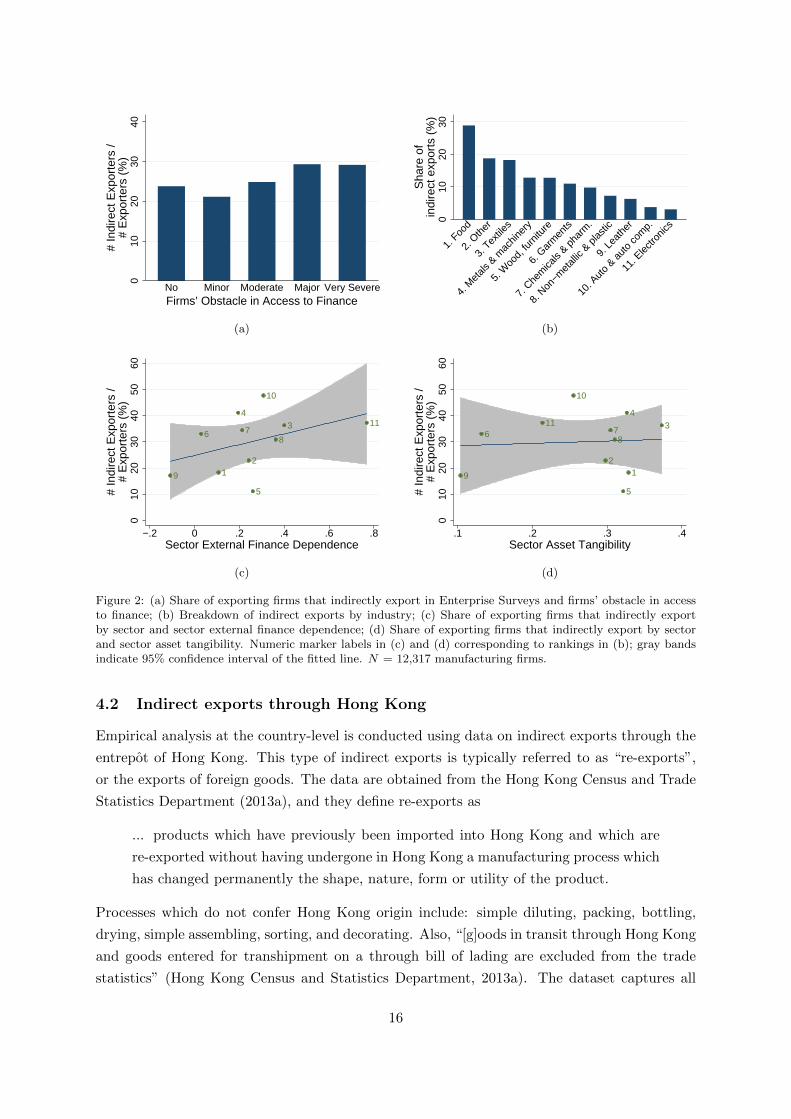
Figure 2 presents preliminary evidence of the relationship between financial constraints and

export mode at the firm and sector level. In Figure 2(a), I plot the share of exporters that

export indirectly across the different levels of financing barriers. While the percentages are

close, there is positive correlation between the severity of credit constraints and the likelihood

of exporting indirectly, as one might expect from the theory.

Next, Figure 2(b) graphs the use of domestic intermediaries across industries in the raw data.

For each country, each industry’s share of total indirect exports is computed; the unweighted

mean of all countries is presented. Although the share of indirect exports that are in industries

manufacturing food and textile products are indeed large, there is still a considerable amount

of indirect exports in other industries. In particular, the percentages for Metals and Machinery

as well as Wood and Furniture are both greater than 10%.

Lastly, Figures 2(c) and (d) plot the share of exporters that export indirectly across different

levels of sector financial vulnerability. Financially vulnerability is characterized by high external

finance dependence and low asset tangibility (see Section 4.3 below). In the model, exporting

firms in financially vulnerable sectors are also more likely to be export through intermediaries

(∂ Pr(indirect|exporter)/∂ηs > 0), so we expect a positive (negative) relationship between

external finance dependence (asset tangibility) and the likelihood of exporting indirectly. While

Figure 2(b) examines sales, (c) and (d) are focused on the proportion of indirect exporting firms.

The numeric marker labels beside each observation correspond to the rank of indirect sales in

(b). The positive relationship between the share of indirect exporters and sectors’ dependence

on outside financing is clear, but the raw correlation with asset hardness is weak.

externally, but this variable contains many more missing observations. The correlation with the obstacle indexfor obtaining finance is 0.174, so they are weakly positively correlated. While the regression results using thisvariable are qualitatively similar to the main findings, the coefficients are not precisely estimated.

15

010

2030

40

# In

dire

ct E

xpor

ters

/#

Exp

orte

rs (

%)

No Minor Moderate Major Very SevereFirms’ Obstacle in Access to Finance

(a)

010

2030

Sha

re o

fin

dire

ct e

xpor

ts (

%)

1. F

ood

2. O

ther

3. T

extile

s

4. M

etals

& m

achin

ery

5. W

ood,

furn

iture

6. G

arm

ents

7. C

hem

icals

& pha

rm.

8. N

on−m

etall

ic & p

lastic

9. L

eath

er

10. A

uto

& aut

o co

mp.

11. E

lectro

nics

(b)

3

9

6

1

411

7

5

8

10

2

010

2030

4050

60

# In

dire

ct E

xpor

ters

/#

Exp

orte

rs (

%)

−.2 0 .2 .4 .6 .8Sector External Finance Dependence

(c)

3

9

6

1

411

7

5

8

10

2

010

2030

4050

60

# In

dire

ct E

xpor

ters

/#

Exp

orte

rs (

%)

.1 .2 .3 .4Sector Asset Tangibility

(d)

Figure 2: (a) Share of exporting firms that indirectly export in Enterprise Surveys and firms’ obstacle in accessto finance; (b) Breakdown of indirect exports by industry; (c) Share of exporting firms that indirectly exportby sector and sector external finance dependence; (d) Share of exporting firms that indirectly export by sectorand sector asset tangibility. Numeric marker labels in (c) and (d) corresponding to rankings in (b); gray bandsindicate 95% confidence interval of the fitted line. N = 12,317 manufacturing firms.

4.2 Indirect exports through Hong Kong

Empirical analysis at the country-level is conducted using data on indirect exports through the

entrepot of Hong Kong. This type of indirect exports is typically referred to as “re-exports”,

or the exports of foreign goods. The data are obtained from the Hong Kong Census and Trade

Statistics Department (2013a), and they define re-exports as

... products which have previously been imported into Hong Kong and which are

re-exported without having undergone in Hong Kong a manufacturing process which

has changed permanently the shape, nature, form or utility of the product.

Processes which do not confer Hong Kong origin include: simple diluting, packing, bottling,

drying, simple assembling, sorting, and decorating. Also, “[g]oods in transit through Hong Kong

and goods entered for transhipment on a through bill of lading are excluded from the trade

statistics” (Hong Kong Census and Statistics Department, 2013a). The dataset captures all

16

1020

3040

5060

Sha

re o

f Exp

orts

thro

ugh

Hon

g K

ong

(%)

1860 1880 1900 1920 1940 1960 1980 2000Year

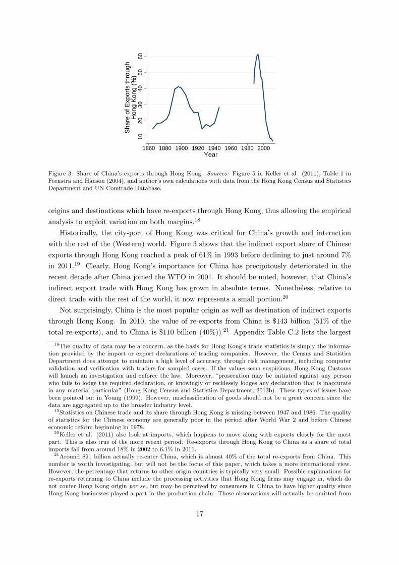
Figure 3: Share of China’s exports through Hong Kong. Sources: Figure 5 in Keller et al. (2011), Table 1 inFeenstra and Hanson (2004), and author’s own calculations with data from the Hong Kong Census and StatisticsDepartment and UN Comtrade Database.

origins and destinations which have re-exports through Hong Kong, thus allowing the empirical

analysis to exploit variation on both margins.18

Historically, the city-port of Hong Kong was critical for China’s growth and interaction

with the rest of the (Western) world. Figure 3 shows that the indirect export share of Chinese

exports through Hong Kong reached a peak of 61% in 1993 before declining to just around 7%

in 2011.19 Clearly, Hong Kong’s importance for China has precipitously deteriorated in the

recent decade after China joined the WTO in 2001. It should be noted, however, that China’s

indirect export trade with Hong Kong has grown in absolute terms. Nonetheless, relative to

direct trade with the rest of the world, it now represents a small portion.20

Not surprisingly, China is the most popular origin as well as destination of indirect exports

through Hong Kong. In 2010, the value of re-exports from China is $143 billion (51% of the

total re-exports), and to China is $110 billion (40%)).21 Appendix Table C.2 lists the largest

18The quality of data may be a concern, as the basis for Hong Kong’s trade statistics is simply the informa-tion provided by the import or export declarations of trading companies. However, the Census and StatisticsDepartment does attempt to maintain a high level of accuracy, through risk management, including computervalidation and verification with traders for sampled cases. If the values seem suspicious, Hong Kong Customswill launch an investigation and enforce the law. Moreover, “prosecution may be initiated against any personwho fails to lodge the required declaration, or knowingly or recklessly lodges any declaration that is inaccuratein any material particular” (Hong Kong Census and Statistics Department, 2013b). These types of issues havebeen pointed out in Young (1999). However, misclassification of goods should not be a great concern since thedata are aggregated up to the broader industry level.

19Statistics on Chinese trade and its share through Hong Kong is missing between 1947 and 1986. The qualityof statistics for the Chinese economy are generally poor in the period after World War 2 and before Chineseeconomic reform beginning in 1978.

20Keller et al. (2011) also look at imports, which happens to move along with exports closely for the mostpart. This is also true of the more recent period. Re-exports through Hong Kong to China as a share of totalimports fall from around 18% in 2002 to 6.1% in 2011.

21Around $91 billion actually re-enter China, which is almost 40% of the total re-exports from China. Thisnumber is worth investigating, but will not be the focus of this paper, which takes a more international view.However, the percentage that returns to other origin countries is typically very small. Possible explanations forre-exports returning to China include the processing activities that Hong Kong firms may engage in, which donot confer Hong Kong origin per se, but may be perceived by consumers in China to have higher quality sinceHong Kong businesses played a part in the production chain. These observations will actually be omitted from

17

(a)

01

23

45

Sha

re o

f Exp

orts

thro

ugh

Hon

g K

ong

(%)

45

67

89

10

(log)

Rea

l Ind

irect

Exp

orts

and

Exp

orts

(bi

llion

s of

200

5 U

SD

)

2002 2004 2006 2008 2010 2012

Re−exports through Hong KongBilateral exportsShare of exports through HongKong

(b)

010

2030

40S

hare

of r

e−ex

port

s (%

)

Mac

hiner

y, ele

ctric

Mac

hiner

y, ex

cept

elec

trica

l

Other

Prof.

and

scien

t. eq

uipm

ent

Textile

s

Garm

ents

Indu

strial

chem

icals

Plastic

pro

ducts

Leat

her

Other

chem

icals

(c)

050

100

Indi

rect

Exp

ort S

hare

(%

)

0 100 200 300Private credit−to−GDP ratio

(d)

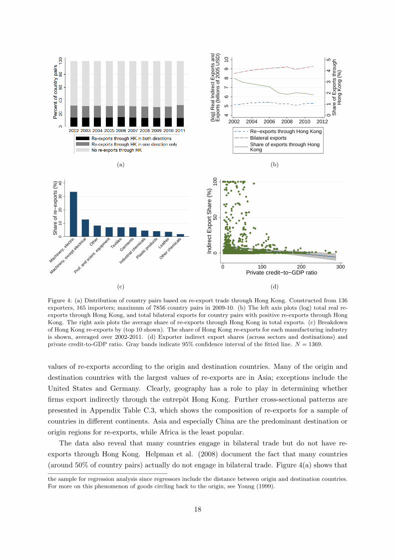
Figure 4: (a) Distribution of country pairs based on re-export trade through Hong Kong. Constructed from 136exporters, 165 importers; maximum of 7856 country pairs in 2009-10. (b) The left axis plots (log) total real re-exports through Hong Kong, and total bilateral exports for country pairs with positive re-exports through HongKong. The right axis plots the average share of re-exports through Hong Kong in total exports. (c) Breakdownof Hong Kong re-exports by (top 10 shown). The share of Hong Kong re-exports for each manufacturing industryis shown, averaged over 2002-2011. (d) Exporter indirect export shares (across sectors and destinations) andprivate credit-to-GDP ratio. Gray bands indicate 95% confidence interval of the fitted line. N = 1369.

values of re-exports according to the origin and destination countries. Many of the origin and

destination countries with the largest values of re-exports are in Asia; exceptions include the

United States and Germany. Clearly, geography has a role to play in determining whether

firms export indirectly through the entrepot Hong Kong. Further cross-sectional patterns are

presented in Appendix Table C.3, which shows the composition of re-exports for a sample of

countries in different continents. Asia and especially China are the predominant destination or

origin regions for re-exports, while Africa is the least popular.

The data also reveal that many countries engage in bilateral trade but do not have re-

exports through Hong Kong. Helpman et al. (2008) document the fact that many countries

(around 50% of country pairs) actually do not engage in bilateral trade. Figure 4(a) shows that

the sample for regression analysis since regressors include the distance between origin and destination countries.For more on this phenomenon of goods circling back to the origin, see Young (1999).

18

of countries with positive trade flows, either directly with one another or indirectly through

Hong Kong, the majority of country pairs do not trade through Hong Kong. Some 20% have

positive indirect exports through Hong Kong in one direction, while around 15% have it in both

directions.22 This pattern of the extensive margin is very stable over these 10 years.

Figure 4(b) shows how the intensive margin of the re-export trade in Hong Kong has changed

over time. On the left axis of Figure 4(b), the value of (log) total re-exports through Hong Kong

is plotted. Of country pairs with positive indirect exports through Hong Kong, their bilateral

direct exports is aggregated globally and shown as well. Values of (gross) exports come from

the UN Comtrade Database. While both trade flows experience a net increase over this period,

direct exports certainly rise more than indirect exports. This is consistent with the evidence of

trade barriers gradually declining, whether in the form of tariffs or physical impediments such as

transportation costs. Appendix Figure C.1 displays regional heterogeneity. Re-exports through

Hong Kong have increased significantly (at roughly 78%) for Asian destinations, including

China. Meanwhile, re-exports to Africa have risen by 63%. The effect of the 2007-08 Financial

Crisis is also clear. Re-exports generally fell, especially in 2009, then recovered thereafter.

Europe and the United States faced the largest declines in 2009 as importers, and also had

the slowest rebounds. Of course, global trade flows greatly diminished as a whole during this

period. In 2009, re-exports fell by more than 16%, but direct exports contracted even more at

21%. On the right axis of Figure 4(b), the share of exports that flow through Hong Kong as

re-exports is plotted. The overall trend is a decline from over 3% to less than 2%, but with an

increase in 2009 before falling again. Appendix Table C.4 presents re-export shares in 2010 for

various countries to and from regions. For China, around 9% of exports to the rest of Asia as

well as Europe or the Americas are intermediated by Hong Kong.23

Figure 4(c) shows the breakdown of indirect exports by industry. Again, the classification

of an industry is 3-digit ISIC Rev. 2.24 There are 25 industries in the data analysis.25 For

each year, each industry’s proportion of total re-exports through Hong Kong is computed;

averages over 2002 to 2011 for the top 10 industries are shown. The pattern in any one year is

similar as the standard deviation across years is not large. As in Figure 2(b), other industries

besides Textiles and Wearing apparel represent a large portion of indirect exports. In fact, both

Machinery sectors, electrical and non-electrical, are consistently the top industries.

Finally, Figure 4(d) provides a first glance at the relationship between countries’ strength

of financial institutions and their indirect export share from intermediary trade through Hong

Kong. Financial development is measured by the commonly used private credit-to-GDP ratio

22In 2010, there were 83 country pairs with positive re-exports through Hong Kong but zero direct exports.23The statistics of Appendix Table C.4 are similar if we calculate re-export shares to each destination/origin

first, then take the average over the region.24The original classification of Hong Kong re-exports is 5-digit SITC (Rev. 3 and Rev. 4). The UN Statistics

Division provides tables for converting higher revisions of SITC, namely Rev. 4 and Rev. 3, to Rev. 2.25These are: Food (ISIC Rev. 2 311, 312), Beverages (313), Textiles (321), Garments (322), Leather (323),

Wood except furniture (331), Furniture except metal (332), Paper and products (341), Printing and publishing(342), Industrial chemicals (351), Other chemicals (352), Rubber products (355), Plastic products (356), Pottery,china, earthenware (361), Glass and products (362), Other non-metallic products (369), Iron and steel (371),Non-ferrous metals (372), Fabricated metal products (381), Machinery except electrical (382) Machinery, electric(383), Transport equipment (384), Professional and scientific equipment (385), and Other (390).

19

(see Section 4.4). A clear negative correlation is displayed, as more financially developed coun-

tries have lower indirect export shares. The correlation is also statistically significant, as the

t-statistic from a simple OLS regression is -4.91, and with year fixed effects included, -4.35.

4.3 Sector characteristics

Measures of financial vulnerability are drawn from standard sources. Rajan and Zingales (1998)

provides the measure for external finance dependence, defined as capital expenditures minus

cash flow from operations divided by capital expenditures. In other words, this is the share

of investment needs that cannot be financed with the firm’s internal funds. The measure for

asset tangibility is taken from Braun (2003), defined as net property, plant, and equipment

over total assets. This captures the ability of of an firm in a particular industry to secure

external finance by pledging collateralizable assets. The mean (standard deviation) of external

finance dependence across industries is 0.24 (0.33), while for asset tangibility it is 0.30 (0.14).

The correlation between them is low (0.0096), demonstrating they capture different aspects of

financial vulnerability.

Both external finance dependence and asset tangibility measures are constructed using data

from publicly listed US companies in Compustat. The industry median is chosen to summa-

rize financial vulnerability across firms. The measures reflect large technological components

associated with industries’ demand for external financing and overall asset hardness (Rajan

and Zingales 1998, Claessens and Laeven 2003). Therefore, they are regarded as exogenous

from the perspective of individual firms. As noted by authors who have previously used these

variables, there are certain advantages to using US data for measurement (Braun 2003, Manova

2008, 2013). Since US financial institutions are highly developed, this implies firms can closely

attain their optimal quantity of external financing and asset structure. Moreover, the choice

of a reference country mitigates endogeneity for country-level regressions. While the levels of

these measures may vary for each country, identification requires that the ranking of sectors is

similar across countries. Lastly, to the extent that the costs of production in manufacturing

and distribution or marketing costs for domestic and foreign markets are comparable, the use

of financial vulnerability as a measure of the cost arising from financial frictions is applicable

to both producing for the domestic market and exporting abroad.

4.4 Country characteristics

Data for country-level explanatory variables are obtained from various sources. Following previ-

ous studies (e.g., Rajan and Zingales 1998, Claessens and Laeven 2003, Braun 2003, and Manova

2013), a country’s level financial development is proxied with private credit by deposit money

banks (as a percentage of GDP) from Beck et al. (2000). This is an outcome-based measure

that captures the use of external funds in an economy.26 Real GDP is computed from the IMF

World Economic Outlook Database. As standard practice, geographic distance is used as the

26Taiwan is not in this dataset, so I follow the methodology of Beck et al. (2000) and use financial statisticsdata from the Central Bank of the Republic of China (Taiwan) (2013).

20

proxy for iceberg variable transportation costs. The measure of geographic distance between

countries is drawn from CEPII (Mayer and Zignago 2011).27

The proxy for the fixed cost of exporting is constructed from the World Bank Doing Business

reports data. In this dataset, there are three separate measures of the cost of trade across

borders: the number of documents, time, and cost (per container) of exporting or importing.

These are commonly employed as measures of trade costs in the international trade literature

(e.g., Bernard et al. 2013, Chan and Manova 2014), and they do not depend on the value of

shipment or quantity of exports. I compute an index that takes the average of all three, with a

higher value indicating larger bilateral fixed costs of trade for a given country pair.

Other country-level variables include the strength of the contracting environment and tax

rates. Rule of law from the World Bank Governance Indicators is used to measure the strength

of a country’s contracting environment, while data on corporate tax rates is retrieved from

KPMG International (2013).28 Lastly, bilateral tariff data at the ISIC 3-digit indudstry level

are retrieved from the World Integrated Trade Solution (WITS) TRAINS database.29

5 Empirical results

5.1 Firm-level evidence

5.1.1 Productivity sorting

Results from the ordered probit regression of Equation (3.1) are shown in Table 2. The sample

includes all manufacturing firms for 118 countries. Labor productivity is measured by value

added per employee, where value added is sales minus the cost of raw materials and inter-

mediated goods used in production. Due to data limitations, two measures of productivity

are typically employed when examining the Enterprise Surveys: sales per employee and value

added per employee. The number of observations is greatly reduced when using total factor

productivity (TFP), so the main results presented here rely on (log) value added per worker.

The regression results are qualitatively identical using either sales per employee or TFP as

measures of productivity; these are available upon request.30 The number of employees is per-

manent plus temporary workers (weighted by average length of employment). Standard errors

are clustered by strata, but similar results are obtained if they are instead clustered by sector

or country-sector.

The results are supportive of Proposition 1, firms’ productivity sorting pattern. The co-

27Simple distance (most populated cities, km) is used.28While some of these values may differ from say the OECD, they are explicit about why such differences may

arise. For example, the marginal federal corporate income tax rate on the highest income bracket of corporationsin the United States is 35%, but the effective rate including state and local taxes and deductibles is approximately40%.

29The duty type is effectively applied rates.30To construct TFP, the measure of capital is the net book value of machinery vehicles, equipment, land, and

buildings. TFP is the residual from the constrained log-log regression of sales per worker or value added perworker on capital and number of workers with country, sector, and year fixed effects. The correlation of (log)value added per employee with (log) sales per employee and TFP are 0.970 and 0.653 respectively.

21

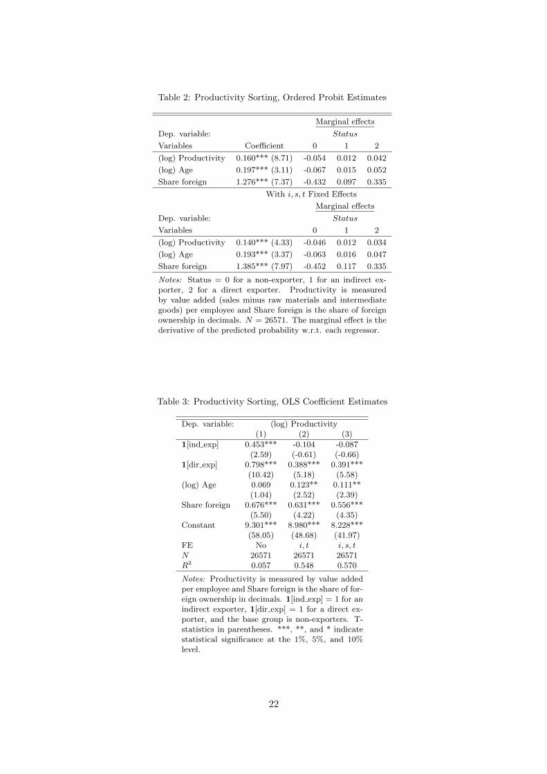
Table 2: Productivity Sorting, Ordered Probit Estimates

Marginal effects

Dep. variable: Status

Variables Coefficient 0 1 2

(log) Productivity 0.160*** (8.71) -0.054 0.012 0.042

(log) Age 0.197*** (3.11) -0.067 0.015 0.052

Share foreign 1.276*** (7.37) -0.432 0.097 0.335

With i, s, t Fixed Effects

Marginal effects

Dep. variable: Status

Variables 0 1 2

(log) Productivity 0.140*** (4.33) -0.046 0.012 0.034

(log) Age 0.193*** (3.37) -0.063 0.016 0.047

Share foreign 1.385*** (7.97) -0.452 0.117 0.335

Notes: Status = 0 for a non-exporter, 1 for an indirect ex-porter, 2 for a direct exporter. Productivity is measuredby value added (sales minus raw materials and intermediategoods) per employee and Share foreign is the share of foreignownership in decimals. N = 26571. The marginal effect is thederivative of the predicted probability w.r.t. each regressor.

Table 3: Productivity Sorting, OLS Coefficient Estimates

Dep. variable: (log) Productivity(1) (2) (3)

1[ind exp] 0.453*** -0.104 -0.087(2.59) (-0.61) (-0.66)

1[dir exp] 0.798*** 0.388*** 0.391***(10.42) (5.18) (5.58)

(log) Age 0.069 0.123** 0.111**(1.04) (2.52) (2.39)

Share foreign 0.676*** 0.631*** 0.556***(5.50) (4.22) (4.35)

Constant 9.301*** 8.980*** 8.228***(58.05) (48.68) (41.97)

FE No i, t i, s, tN 26571 26571 26571R2 0.057 0.548 0.570

Notes: Productivity is measured by value addedper employee and Share foreign is the share of for-eign ownership in decimals. 1[ind exp] = 1 for anindirect exporter, 1[dir exp] = 1 for a direct ex-porter, and the base group is non-exporters. T-statistics in parentheses. ***, **, and * indicatestatistical significance at the 1%, 5%, and 10%level.

22

efficients on (log) productivity in both panels are positive and statistically significant, which

suggests that more productive firms are more likely to be direct exporters and less likely to only

sell in the home market. An increase in productivity also increases the probability of being an

indirect exporter, as indicated by the marginal effect of productivity when Status is equal to 1.

Marginal effects are calculated by taking derivative of the predicted probability with respect to

each regressor. The bottom panels include country, industry, and year fixed effects, and reveals

the same qualitative pattern. With this specification, the predicted conditional probabilities

of pure domestic production, indirect exporting, and direct exporting are respectively 0.737,

0.105, and 0.158. When firm productivity improves by 10%, the likelihood of being a indirect

exporter and direct exporter increases respectively by 0.12% and 0.34%. Along with productiv-

ity, firm age and the share of foreign ownership also increase the probability of exporting. Both

coefficients are positive and statistically significant in either panel of Table 2. Similar results

are obtained with an ordered logit model.

Estimates in the bottom panels of Table 2 are potentially inconsistent and/or biased due

to the incidental parameters problem for non-linear models with unobserved effects.31 Thus, I

present results from an alternative approach to test the productivity sorting pattern: an OLS

regression of productivity on indicator variables for indirect and direct exporting. The following

equation is estimated:

lnProdfsit = b0 + b11[ind exp]fsit + b21[dir exp]fsit + bZZfsit + cs + ci + ct + efsit. (5.1)

Table 3 displays the results. While direct exporters certainly appear to be the most productive,

the distinction in productivity between indirect exporters and non-exporters is less apparent.

With sector, country, and year fixed effects in columns 2 or 3, the coefficient on the indirect

exporter dummy variable is negative but imprecisely estimated. Measuring labor productivity

with sales per employee, the coefficient on the indirect exporting indicator is positive but the

standard error is also large. The findings here suggest that empirically, for this sample of

developing countries, indirect exporters may only be marginally more productive than non-

exporting producers, if at all.

5.1.2 Financial constraints and export mode

Besides Proposition 2, the model also predicts that financially constrained firms are more likely

to be pure domestic producers and not export abroad. In unreported results, I confirm that

FinCons actually does not have a significant effect on the likelihood of exporting. This is in

fact consistent with the findings in Table 3. If cutoff productivities ϕHiis and ϕIijs are equal, then

the model predicts that financial constraints have no effect on the probability of exporting.

Furthermore, it may be that financial constraints prevent firms from selling to less profitable

destinations, but they still manage to sell to some highly attractive markets, in which case they

are still classified as exporters. Unfortunately, the Enterprise Surveys do not provide detailed

31While the Chamberlain-Mundlak device could theoretically be used, to the best of my knowledge, there isno estimator for random-effects ordered probit or logit models with sample weights.

23

Table 4: Firm Financial Constraints and Export Mode, Probit Coefficient Estimates

Dependent variable: 1[ind exp](1) (2) (3) (4) (5)

FinCons 0.130** 0.112* 0.136** 0.119* 0.114**(2.04) (1.75) (2.17) (1.89) (1.96)

ExtFins -0.041 -0.201** -0.217**(-0.61) (-2.15) (-2.40)

Tangs 0.053 0.171* 0.140(0.81) (1.85) (1.59)

FinCons × ExtFins 0.149** 0.127** 0.178***(2.50) (2.32) (3.18)

FinCons × Tangs -0.107** -0.082* -0.123**(-2.05) (-1.72) (-2.56)

(log) Productivity -0.202*** -0.171*** -0.189*** -0.172*** -0.170***(-2.98) (-3.04) (-2.93) (-3.03) (-2.69)

(log) L -0.341***(-5.69)

FE i, t i, s, t i, t i, s, t i, tN 9084 9084 9084 9084 9084

Notes: 1[ind exp] = 1 for an indirect exporter, 0 for a direct exporter. Sampleincludes only exporting firms. ExtF ins and Tangs standardized. All regressionsinclude controls for productivity (value added per worker), age of firm, and shareof foreign ownership. T-statistics in parentheses. ***, **, and * indicate statisticalsignificance at the 1%, 5%, and 10% level.

information on the destinations of firm exports. This is less problematic when studying the

choice of export mode among exporting firms since the percentage of firms that have both

positive indirect and direct exports is relatively small. Thus, the analysis proceeds by examining

closely the relation between firm-level financial constraints and export mode.

Table 4 reports the results from estimating Equations (3.2a) and (3.2b), where the sample

is exporting firms only. The empirical results are consistent with Proposition 2: financially

more constrained exporting firms are more likely to be indirect exporters. In all columns of

Table 4, the coefficient of FinCons (γ1) is positive and significant, suggesting that having

greater obstacles in access to finance is positively correlated with indirect exporting. In column

2, which controls for unobserved sector heterogeneity, when FinCons increases by one standard

deviation (1.31), the probability of an exporting firm being an indirect exporter increases by

around 4.8%. All regressions also include as regressors (log) productivity as measured by value

added per worker, firm age, and the share of foreign ownership. Consistent with the productivity

sorting patterns exhibited in Tables 2 and 3, more productive firms are more likely to be direct

exporters.

The results also reveal important systematic variation in the likelihood of indirect exporting

from differences in sector financial vulnerability. Financially constrained exporting firms are

especially likely to export through intermediaries in financially more vulnerable sectors that

rely more on external finance and have soft, less tangible assets. In column 3, industry external

finance dependence (ExtF ins) as well as asset tangibility (Tangs) are included. To ease the in-

terpretation of these coefficients, both have been standardized to mean 0 and standard deviation

1. The coefficients on the interaction terms FinCons × ExtF ins (γ2) and FinCons × Tangs

24

(γ3) are positive and negative respectively, just as the model predicts. Moreover, a one-standard

deviation change in either ExtFins or Tangs changes the marginal effect of FinCons consid-

erably, as the magnitudes of the coefficients on the interaction terms are comparable to that of

FinCons alone.

While firm financial constraints may partially capture the financial vulnerability of the

industry to which it belongs, the correlation between the average level of financial constraints

in a sector and ExtF ins (Tangs) is -0.071 (-0.019), so at first glance there is weak empirical

support for this notion. Regardless, column 4 shows that the main result is robust to the

inclusion of sector fixed effects. Other than financial vulnerability, sector fixed effects subsume

other characteristics like product specificity, contract intensity, or the cost of marketing and

distribution. The effect of financial constraints is mitigated in magnitude but the coefficients

remain significant. Lastly, column 5 in Table 4 controls for firm size with (log) number of

employees as a regressor. Correlation between size and financial constraints is weak at -0.080;

the same is also true for the correlation between size and productivity (-0.028). As one would

expect, larger firms are less likely to be indirect exporters. More importantly, after controlling

for firm size, the key result with regards to FinCons× ExtFins and FinCons× Tangs is not

affected.

Table 5 presents results from alternative estimation methods and other robustness checks.

These estimation results all reinforce the previous empirical findings. Columns 1 shows the

results from estimating a logit model. In column 2, the same method from Papke and Wooldridge

(2008) as described in Section 3.2 is employed. The estimation technique is applicable not just to

continuous fractional dependent variables but binary dependent variables (e.g., indirect versus

direct exporting) as well. Again, the Chamberlain-Mundlak device is used, and comparing

column 3 in Table 4 with column 2 in Table 5, the magnitudes of the coefficients are in fact

very close. Column 3 estimates a simple OLS regression with fixed effects. Estimating this

linear model, the incidental parameters problem is not encountered. Alternatively, the OLS

regression can have the ratio of indirect exports to total exports as the dependent variable.

Since the percentage of firms with both positive indirect and direct exports is relatively small,

many of the values of the dependent variable are 0 or 1. Hence, the coefficient estimates from

such a regression are quantitatively similar, and demonstrate that financially more constrained

firms also have larger shares of sales as indirect exports. Again, this is more pronounced in

financially vulnerable sectors.32

Accounting for potential selection effects into exporting, in columns 4 and 5, results from

estimating a bivariate probit model with selection are reported. Column 4 is the selection

equation while column 5 is the equation of interest which includes the interaction terms. To

satisfy the exclusion restriction, the selection equation in column 4 includes a dummy variable

for having exported in the past, and empirically it is a strong indicator of whether the firm

32With an instrumental variables approach and assuming linearity for computational purposes, the results arequalitatively similar but the coefficients are imprecisely estimated. Following Fisman and Svensson (2007) andOlney (2014), the instrument for financial constraints is the average level of financial constraints of other firmsin the same country, industry, and year.

25

Table 5: Robustness Checks, Alternative Estimation Methods and Additional Controls

Logit Chamberlain OLS Heckman Probit(1) (2) (3) (4) (5) (6) (7)

FinCons 0.235** 0.134** 0.044** 0.001 0.137** 0.188*** 0.185***(2.17) (2.20) (2.26) (0.02) (2.18) (2.67) (2.63)

ExtFins -0.331** -0.200** -0.064** 0.024 -0.198** -0.196***(-2.05) (-2.15) (-2.28) (0.76) (-2.12) (-2.18)

Tangs 0.288* 0.169* 0.057* 0.211** 0.170* 0.166*(1.80) (1.83) (1.86) (2.47) (1.85) (1.86)

FinCons × ExtFins 0.249** 0.148** 0.048*** 0.148** 0.145**(2.24) (2.36) (2.65) (2.49) (2.48)

FinCons × Tangs -0.179* -0.105** -0.036** -0.107** -0.109**(-1.94) (-1.96) (-2.08) (-2.05) (-2.14)

Exported before 6.005***(29.7)

Transportation of goods -0.034 -0.017(-0.37) (-0.19)

Customs, trade regulations -0.055 -0.062(-0.75) (-0.87)

Tax rates -0.017 -0.003(-0.22) (-0.04)

Tax administrations 0.026 0.034(0.34) (0.46)

Labor regulations -0.027 -0.027(-0.28) (-0.27)

Workforce -0.046 -0.043(-0.63) (-0.59)

Crime, theft, and disorder -0.124** -0.135**(-2.07) (-2.33)

Corruption -0.040 -0.032(-0.61) (-0.49)

FE i, t i, t i, t i, t i, t i, t i, tN 9084 9084 9084 26571 26571 9084 9084R2 0.177

Notes: The dependent variable in all columns except column 4 is 1[ind exp]; in column 4 it is an indicator forexporting. Sample includes firms in all columns except column 4, which includes all firms. All regressions includecontrols for productivity, age of firm, and share of foreign ownership. “Workforce” stands for inadequately edu-cated workforce. T-statistics in parentheses. ***, **, and * indicate statistical significance at the 1%, 5%, and10% level.

currently exports. Column 5 shows that previous results are robust to this specification as well.

Columns 6 and 7 in Table 5 reveal that access to finance is the key firm-level obstacle to

business operations correlated with export mode. Recall Table 1 listed the obstacles to business

operations that the Enterprise Surveys inquired about. Including them as regressors, we find

that only the coefficients of access to finance and crime, theft, and disorder are statistically

significant. The p-value from a Wald test of the null hypothesis that all coefficients except

FinCons are zero is 0.269. In particular, the insignificance on the coefficient of Corruption

contrasts with the results of Olney (2014). The findings here suggest that distortions in capital

markets have the strongest relationship with firms’ export modes, while taxes or labor market

frictions are less relevant.

26

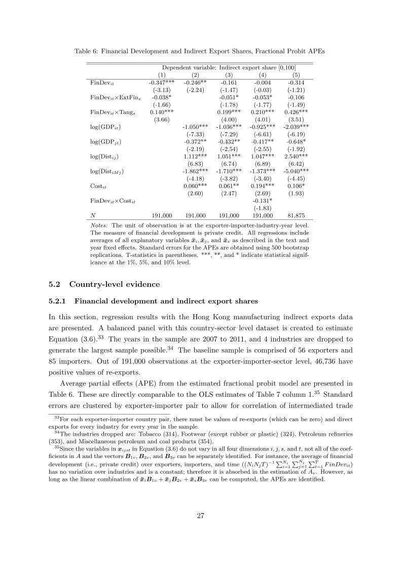
Table 6: Financial Development and Indirect Export Shares, Fractional Probit APEs

Dependent variable: Indirect export share [0,100](1) (2) (3) (4) (5)

FinDevit -0.347*** -0.246** -0.161 -0.004 -0.314(-3.13) (-2.24) (-1.47) (-0.03) (-1.21)

FinDevit×ExtFins -0.038* -0.051* -0.053* -0.106(-1.66) (-1.78) (-1.77) (-1.49)

FinDevit×Tangs 0.140*** 0.199*** 0.210*** 0.426***(3.66) (4.00) (4.01) (3.51)

log(GDPit) -1.050*** -1.036*** -0.925*** -2.039***(-7.33) (-7.29) (-6.61) (-6.19)

log(GDPjt) -0.372** -0.432** -0.417** -0.648*(-2.19) (-2.54) (-2.55) (-1.92)

log(Distij) 1.112*** 1.051*** 1.047*** 2.540***(6.83) (6.74) (6.89) (6.42)

log(DistiMj) -1.862*** -1.710*** -1.373*** -5.040***(-4.18) (-3.82) (-3.40) (-4.45)

Costit 0.060*** 0.061** 0.194*** 0.106*(2.60) (2.47) (2.69) (1.93)

FinDevit×Costit -0.131*(-1.83)

N 191,000 191,000 191,000 191,000 81,875

Notes: The unit of observation is at the exporter-importer-industry-year level.The measure of financial development is private credit. All regressions includeaverages of all explanatory variables xi, xj , and xs as described in the text andyear fixed effects. Standard errors for the APEs are obtained using 500 bootstrapreplications. T-statistics in parentheses. ***, **, and * indicate statistical signif-icance at the 1%, 5%, and 10% level.

5.2 Country-level evidence

5.2.1 Financial development and indirect export shares

In this section, regression results with the Hong Kong manufacturing indirect exports data

are presented. A balanced panel with this country-sector level dataset is created to estimate

Equation (3.6).33 The years in the sample are 2007 to 2011, and 4 industries are dropped to

generate the largest sample possible.34 The baseline sample is comprised of 56 exporters and

85 importers. Out of 191,000 observations at the exporter-importer-sector level, 46,736 have

positive values of re-exports.

Average partial effects (APE) from the estimated fractional probit model are presented in

Table 6. These are directly comparable to the OLS estimates of Table 7 column 1.35 Standard

errors are clustered by exporter-importer pair to allow for correlation of intermediated trade

33For each exporter-importer country pair, there must be values of re-exports (which can be zero) and directexports for every industry for every year in the sample.

34The industries dropped are: Tobacco (314), Footwear (except rubber or plastic) (324), Petroleum refineries(353), and Miscellaneous petroleum and coal products (354).

35Since the variables in xijst in Equation (3.6) do not vary in all four dimensions i, j, s, and t, not all of the coef-ficients in A and the vectors B1v,B2v, and B3v can be separately identified. For instance, the average of financial

development (i.e., private credit) over exporters, importers, and time ((NiNjT )−1 ∑Nii=1

∑Nj

j=1

∑Tt=1 FinDevit)

has no variation over industries and is a constant; therefore it is absorbed in the estimation of Av. However, aslong as the linear combination of xiB1v + xjB2v + xsB3v can be computed, the APEs are identified.

27

across sectors and years for a given set of origin and destination countries.36 All regressions

include averages of all explanatory variables xi, xj , and xs as described in Section 3 as well as

year fixed effects, but these are not reported for ease of exposition. Moreover, the coefficients

have been rescaled by multiplying by 100 so that the indirect export share ranges from 0 to

100 instead of the unit interval. As in the firm-level regressions, both sector external finance

dependence and asset tangibility have been standardized.

The empirical patterns shown in Table 6 are consistent with Proposition 3. As expected,

exporting countries with a higher level of financial development (FinDevit), as measured by the

private credit-to-GDP ratio, are associated with a lower indirect export share. Moreover, the

share of indirect exports varies systematically across sectors as predicted by the model. The

effect of FinDevit on the indirect export share is greater for industries that demand a higher

degree with external finance, as seen by the negative sign on FinDevit×ExtF ins, or industries

with fewer collateralizable assets, as indicated by the positive sign on FinDevit × Tangs. It is

interesting to note that while the micro-level results suggest sector external finance dependence

is a more crucial factor in the determination of export mode, at the aggregate level, it is asset

tangibility that has a larger economic and statistical effect. The stylized model presented in

Section 2 is agnostic about what measures of financial vulnerability should be used. Empirical

results here demonstrate that industry asset tangibility appears to matter more than external

finance dependence in determining the aggregate share of indirect exports.

The key result remains with the inclusion of additional regressors to help alleviate omitted

variable bias. The control variables are standard gravity equation variables such as market

size and distance and the cost of exporting Costit (Costit is standardized). Consistent with the

model’s predictions, the indirect export share is smaller for larger destination markets (GDPjt),

shorter direct distances between origin and destination (log(Distij)), and longer rerouting dis-

tances (log(DistiMj)). The coefficient on Costit is positive and significant, indicating aggregate

indirect export shares are larger when the cost of exporting is higher.37

In column 4, I perform another test of the model by interacting financial development with

the cost of trade. This is similar to the regressions in Becker et al. (2013). The comparative

static tested is ∂2Ψijs/∂θi∂fDij < 0. The intuition for this result, as before, is that the effect

of financial institution strength should be more pronounced when fixed costs are higher. Thus,

this provides a simple test to the model’s assumption that financial frictions amplify fixed

costs and that the effect is multiplicative. The coefficient on the interaction term FinDevit ×Costit is indeed negative as predicted and statistically significant, providing validity to the

model’s assumption. Importantly, the pronounced effect of financial development in financially

36Following Papke and Wooldridge (2008), standard errors are obtained using 500 bootstrap replications.37It is difficult to find a measure that solely captures the cost of selling directly abroad without the cost of

selling indirectly through Hong Kong. However, the model’s prediction ∂Ψijs/∂fDij > 0 holds if one assumes fixed

costs are multiplicative; that is, fDij = fi × fj and fIij = fi × fM . Note that using the cost of importing is alsoproblematic since intermediaries may also have to pay these costs. Regardless, the main finding of the effect offinancial development on indirect export shares is robust to alternative measures of the fixed cost of trade. Inparticular, the World Bank Logistics Performance Index is used as another proxy. For both the Doing Businessmeasure and Logistics Performance Index, the cost of importing and the average of the cost of exporting andimporting have been considered as well. These results are available upon request.

28

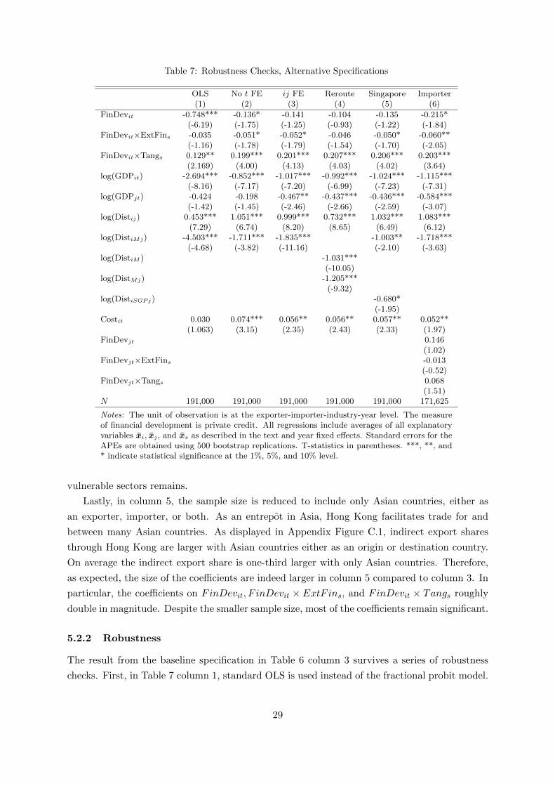
Table 7: Robustness Checks, Alternative Specifications

OLS No t FE ij FE Reroute Singapore Importer(1) (2) (3) (4) (5) (6)

FinDevit -0.748*** -0.136* -0.141 -0.104 -0.135 -0.215*(-6.19) (-1.75) (-1.25) (-0.93) (-1.22) (-1.84)

FinDevit×ExtFins -0.035 -0.051* -0.052* -0.046 -0.050* -0.060**(-1.16) (-1.78) (-1.79) (-1.54) (-1.70) (-2.05)

FinDevit×Tangs 0.129** 0.199*** 0.201*** 0.207*** 0.206*** 0.203***(2.169) (4.00) (4.13) (4.03) (4.02) (3.64)

log(GDPit) -2.694*** -0.852*** -1.017*** -0.992*** -1.024*** -1.115***(-8.16) (-7.17) (-7.20) (-6.99) (-7.23) (-7.31)

log(GDPjt) -0.424 -0.198 -0.467** -0.437*** -0.436*** -0.584***(-1.42) (-1.45) (-2.46) (-2.66) (-2.59) (-3.07)

log(Distij) 0.453*** 1.051*** 0.999*** 0.732*** 1.032*** 1.083***(7.29) (6.74) (8.20) (8.65) (6.49) (6.12)

log(DistiMj) -4.503*** -1.711*** -1.835*** -1.003** -1.718***(-4.68) (-3.82) (-11.16) (-2.10) (-3.63)

log(DistiM ) -1.031***(-10.05)

log(DistMj) -1.205***(-9.32)

log(DistiSGPj) -0.680*(-1.95)

Costit 0.030 0.074*** 0.056** 0.056** 0.057** 0.052**(1.063) (3.15) (2.35) (2.43) (2.33) (1.97)

FinDevjt 0.146(1.02)

FinDevjt×ExtFins -0.013(-0.52)

FinDevjt×Tangs 0.068(1.51)

N 191,000 191,000 191,000 191,000 191,000 171,625

Notes: The unit of observation is at the exporter-importer-industry-year level. The measureof financial development is private credit. All regressions include averages of all explanatoryvariables xi, xj , and xs as described in the text and year fixed effects. Standard errors for theAPEs are obtained using 500 bootstrap replications. T-statistics in parentheses. ***, **, and* indicate statistical significance at the 1%, 5%, and 10% level.

vulnerable sectors remains.

Lastly, in column 5, the sample size is reduced to include only Asian countries, either as

an exporter, importer, or both. As an entrepot in Asia, Hong Kong facilitates trade for and

between many Asian countries. As displayed in Appendix Figure C.1, indirect export shares

through Hong Kong are larger with Asian countries either as an origin or destination country.

On average the indirect export share is one-third larger with only Asian countries. Therefore,

as expected, the size of the coefficients are indeed larger in column 5 compared to column 3. In

particular, the coefficients on FinDevit, F inDevit × ExtF ins, and FinDevit × Tangs roughly

double in magnitude. Despite the smaller sample size, most of the coefficients remain significant.

5.2.2 Robustness

The result from the baseline specification in Table 6 column 3 survives a series of robustness

checks. First, in Table 7 column 1, standard OLS is used instead of the fractional probit model.

29

Note that except for the distance measures log(Distij) and log(DistiMj), the coefficients from

this regression with the averages of the explanatory variables are numerically identical to an

OLS regression with exporter, importer, and sector fixed effects.38 Note that the fractional

probit model estimates of the APEs in Table 6 column 3 are directly comparable to the OLS

estimates. The interaction effects are both underestimated with OLS relative to the fractional

response model, but the signs of the coefficients are the same in either case.

Next, column 2 excludes year fixed effects while column 3 uses country-pair fixed effects as

alternative specifications. The estimates are quantitatively similar to the baseline specification.

Instead of the total rerouting distance, column 4 separates the effects of distance between

the origin to Hong Kong (log(DistiM )) and Hong Kong to the destination (log(DistMj)). Not

surprisingly, both are negatively related to the indirect export ratio, and the magnitudes are

close. As column 5 shows, these results are also robust to the additional control of the rerouting

distances to another nearby entrepot, Singapore. The negative coefficient on DistiSGPj indicates

that when rerouting to Singapore is farther, rather than increasing the share of indirect exports

through Hong Kong, it has the opposite effect of lowering it. This suggests that Hong Kong

may not really be a substitute trading port for Singapore. When transportation costs associated

with rerouting are large, the use of intermediaries in either location is smaller. Lastly, in column

6, financial development of the importing country and its interactions with ExtF ins and Tangs

are included as regressors. There does not appear to be any systematic variation of indirect

export shares across importers’ strength of financial institutions nor across sector financial

vulnerability. Compared with exporter financial development, these effects are small and not

statistically significant. This is consistent with the idea that financial frictions affect export

decisions and intermediaries help exporting firms alleviate these frictions.

Similar qualitative patterns are observed in Table 8, which presents specifications with

additional regressors as motivated by prior literature. Bernard et al. (2013) find indirect exports

are larger with a stronger contracting environment in the importing country. Columns 1 and

2 of Table 8 indicate that the strength of the exporter’s contracting environment ConEnvit is

correlated with indirect export shares through Hong Kong, but not the importer’s. The private

credit-to-GDP ratio and rule of law measures are highly correlated (0.638), so it is not too

surprising to find financial development has less impact when both are included.

The regression in column 3 includes the corporate tax rates of the origin and destination

countries as explanatory variables. Feenstra and Hanson (2004) examine the single origin coun-

try of China and find that destination countries with lower corporate tax rates are associated

with lower re-export shares.39 The results here also show that a lower corporate tax rate in

either the origin or destination country is correlated with smaller re-export shares; however, the

38With a fixed effects model estimated with OLS, the coefficient on log(Distij) remains positive and significantwhile log(DistiMj) is positive but insignificant.

39The idea proposed is that firms with business presence in China and Hong Kong have an incentive to setartificially low prices on Chinese exports to Hong Kong. Since the corporate tax rate is lower in Hong Kong thanin China, firms would like to transfer profits and avoid taxes. The value of re-exports would thus be larger. From2007-2011, Hong Kong has one of the lowest corporate tax rates in the sample. The idea is the same in the caseof transferring profits from the origin country to Hong Kong.

30

Table 8: Robustness Checks, Additional Regressors

Dependent variable: Indirect export share [0,100](1) (2) (3) (4)

FinDevit -0.154 -0.142 -0.151 -0.130(-1.43) (-1.31) (-1.44) (-1.18)

FinDevit×ExtFins -0.043 -0.044 -0.048 -0.054*(-1.59) (-1.59) (-1.76) (-1.95)

FinDevit×Tangs 0.181*** 0.189*** 0.189*** 0.141**(3.89) (3.98) (4.02) (2.34)

log(GDPit) -0.976*** -0.971*** -0.992*** -1.024***(-7.14) (-7.16) (-7.00) (-7.23)

log(GDPjt) -0.421** -0.385** -0.421*** -0.436***(-2.53) (-2.39) (-2.56) (-2.59)

log(Distij) 0.943*** 0.932*** 0.964*** 1.032***(6.81) (6.55) (7.18) (6.49)

log(DistiMj) -1.335*** -1.165*** -1.373*** -1.003**(-3.24) (-3.13) (-3.60) (-2.10)

Costit 0.052* 0.049* 0.080*** 0.043(1.92) (1.83) (2.85) (1.54)

ConEnvit 1.360* 1.440**(1.89) (2.00)

ConEnvjt 0.031(0.06)

Corporate Rateit 0.178(0.83)

Corporate Ratejt 0.252(1.25)

Tariffijst 0.898*(1.69)

N 191,000 191,000 191,000 133,875

Notes: Average partial effects (APE) shown. All regressions includelog(GDPit), log(GDPjt), log(Distij), log(DistiMj), averages of all ex-planatory variables xi, xj , and xs and year fixed effects. Standard er-rors for the APEs are obtained using 500 bootstrap replications.

effects are not precisely estimated. Evidence for corporate tax evasion in this sample appears

to be weak.

Tariffs are another type of trade barrier considered in column 4. Fisman et al. (2008) find

a positive relationship between tariff rates and the re-export share from Hong Kong to China,

suggesting possible tariff evasion through the entrepot of Hong Kong. In terms of the model, a

tariff simply increases variable costs and essentially reduces the effective destination market size.

Both hypotheses suggest that a higher tariff rate should be associated with higher re-export

shares, and this is indeed empirically observed. However, distinguishing the two hypotheses is

beyond the scope of the paper. More importantly, the empirically observed effect of financial

development on indirect export shares is unchanged.

6 Calibration and counterfactuals

To quantitatively evaluate the contribution of trade intermediation on aggregate welfare and

firm performance, I calibrate the model in Section 2 for two countries, China and the US

in 2005, in general equilibrium. The calibration strategy mainly follows Breinlich and Cunat

31

(2011), but also resembles Melitz and Redding (2013). Since indirect exporting is an extra

option for producers, removing trade intermediaries can only hurt producers. Without a clean

natural experiment, it is difficult to assess the importance of trade intermediaries in facilitating

international transactions. From the calibration, the fixed costs of production and exporting

are recovered. I then perform counterfactual exercises by altering the fixed costs and analyze,

through the lends of the model, the effect on consumers and suppliers in various hypothetical

scenarios.

Additional simplifications are introduced to the model in order to match it to the data.

First, there is only one manufacturing sector for differentiated varieties (S = 1). Therefore the

utility function is Uj = q1−µjj0

(∫Ωjs

qjs(ω)σ−1σ dω

) σσ−1

µj. Separate measures of µj are estimated

for China and the US. Pj is the price index for manufacturing goods; the price index for the

whole country combines Pj and the numeraire price of one. Thus, welfare as defined by the real

wage is:40

wj(1

1−µj

)1−µj (Pjµj

)µj . (6.1)

On the supply side, after paying the sunk cost of entry fEii , differentiated goods firms draw

productivity ϕ from a Pareto distribution with support [1,∞), i.e., G(ϕ) = 1−ϕ−k. Wages are

set exogenously in the homogeneous goods sector. Of M ei potential entrants in each country, Mi

firms with productivity greater than or equal to the cutoff productivity ϕHii end up producing

domestically, and a fraction of those firms also export to the rest of the world. This is determined

by a free entry condition which states the probability of successful entry multiplied by the

average profits conditional on successful entry are equal to the (nominal) sunk entry cost:

(1−G(ϕHii ))πi = wifEii , (6.2)

where

πi =1

1−G(ϕHii )

[∫ ∞ϕHii

πHii (ϕ)dG(ϕ) +

∫ ϕij

ϕIij

πIij(ϕ)dG(ϕ) +

∫ ∞ϕij

πDij (ϕ)dG(ϕ)].

Thus, πi includes profits from domestic sales as well as exports; πHii (ϕ), πIij(ϕ), and πDij (ϕ), are

analogs of Equations (2.5a) to (2.5c).

The calibration recovers the fixed costs of domestic production, indirect exporting, and

direct exporting. Table 9 summarizes the one-to-one mapping between fixed costs and observed

aggregate variables or moments after solving the system of equations that describes the two-

country economy and its stationary equilibrium (see Appendix D). Subscripts c and u denote

China and the US respectively. The sunk cost of entry for China (fEcc) is retrieved directly from

the data.

With a homogeneous goods sector, trade in the manufacturing goods sector can be unbal-

anced. Table 10 gives a sense of the amount of trade between the two countries. µiYi represents

40Given the functional form of preferences, defining welfare as the real wage is equivalent using utility.

32

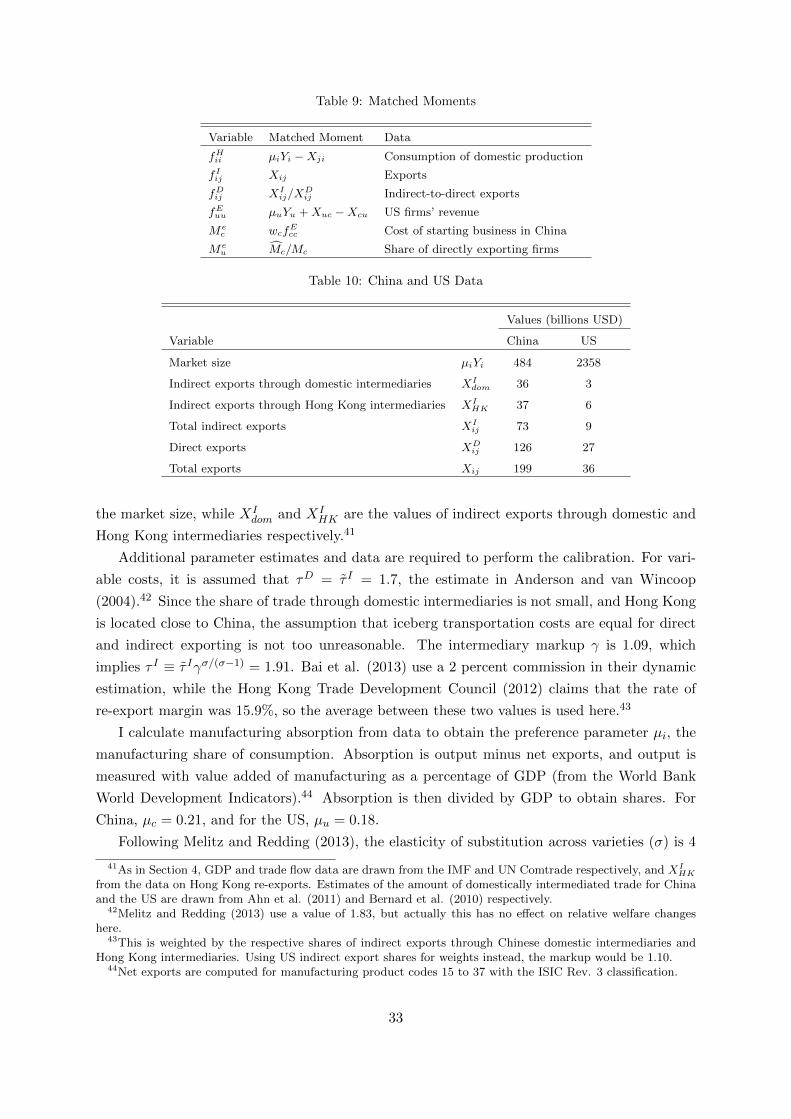
Table 9: Matched Moments

Variable Matched Moment Data

fHii µiYi −Xji Consumption of domestic production

fIij Xij Exports

fDij XIij/X

Dij Indirect-to-direct exports

fEuu µuYu +Xuc −Xcu US firms’ revenue

Mec wcf

Ecc Cost of starting business in China

Meu Mc/Mc Share of directly exporting firms

Table 10: China and US Data

Values (billions USD)

Variable China US

Market size µiYi 484 2358

Indirect exports through domestic intermediaries XIdom 36 3

Indirect exports through Hong Kong intermediaries XIHK 37 6

Total indirect exports XIij 73 9

Direct exports XDij 126 27

Total exports Xij 199 36

the market size, while XIdom and XI

HK are the values of indirect exports through domestic and

Hong Kong intermediaries respectively.41

Additional parameter estimates and data are required to perform the calibration. For vari-

able costs, it is assumed that τD = τ I = 1.7, the estimate in Anderson and van Wincoop

(2004).42 Since the share of trade through domestic intermediaries is not small, and Hong Kong

is located close to China, the assumption that iceberg transportation costs are equal for direct

and indirect exporting is not too unreasonable. The intermediary markup γ is 1.09, which

implies τ I ≡ τ Iγσ/(σ−1) = 1.91. Bai et al. (2013) use a 2 percent commission in their dynamic

estimation, while the Hong Kong Trade Development Council (2012) claims that the rate of

re-export margin was 15.9%, so the average between these two values is used here.43

I calculate manufacturing absorption from data to obtain the preference parameter µi, the

manufacturing share of consumption. Absorption is output minus net exports, and output is

measured with value added of manufacturing as a percentage of GDP (from the World Bank

World Development Indicators).44 Absorption is then divided by GDP to obtain shares. For

China, µc = 0.21, and for the US, µu = 0.18.

Following Melitz and Redding (2013), the elasticity of substitution across varieties (σ) is 4

41As in Section 4, GDP and trade flow data are drawn from the IMF and UN Comtrade respectively, and XIHK

from the data on Hong Kong re-exports. Estimates of the amount of domestically intermediated trade for Chinaand the US are drawn from Ahn et al. (2011) and Bernard et al. (2010) respectively.

42Melitz and Redding (2013) use a value of 1.83, but actually this has no effect on relative welfare changeshere.

43This is weighted by the respective shares of indirect exports through Chinese domestic intermediaries andHong Kong intermediaries. Using US indirect export shares for weights instead, the markup would be 1.10.

44Net exports are computed for manufacturing product codes 15 to 37 with the ISIC Rev. 3 classification.

33

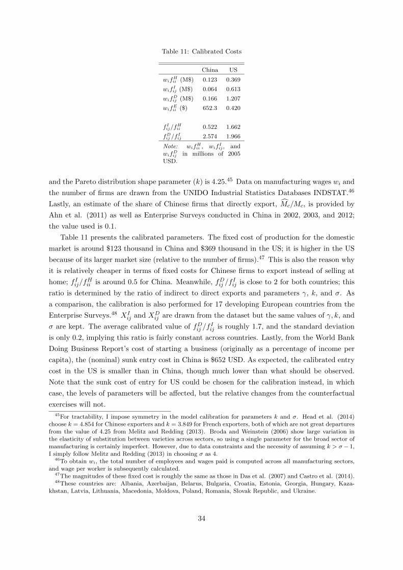
Table 11: Calibrated Costs

China US

wifHii (M$) 0.123 0.369

wifIij (M$) 0.064 0.613

wifDij (M$) 0.166 1.207

wifEii ($) 652.3 0.420

fIij/fHii 0.522 1.662

fDij /fIij 2.574 1.966

Note: wifHii , wif

Iij , and

wifDij in millions of 2005

USD.

and the Pareto distribution shape parameter (k) is 4.25.45 Data on manufacturing wages wi and

the number of firms are drawn from the UNIDO Industrial Statistics Databases INDSTAT.46

Lastly, an estimate of the share of Chinese firms that directly export, Mc/Mc, is provided by

Ahn et al. (2011) as well as Enterprise Surveys conducted in China in 2002, 2003, and 2012;

the value used is 0.1.

Table 11 presents the calibrated parameters. The fixed cost of production for the domestic

market is around $123 thousand in China and $369 thousand in the US; it is higher in the US

because of its larger market size (relative to the number of firms).47 This is also the reason why

it is relatively cheaper in terms of fixed costs for Chinese firms to export instead of selling at

home; f Iij/fHii is around 0.5 for China. Meanwhile, fDij /f

Iij is close to 2 for both countries; this

ratio is determined by the ratio of indirect to direct exports and parameters γ, k, and σ. As

a comparison, the calibration is also performed for 17 developing European countries from the

Enterprise Surveys.48 XIij and XD

ij are drawn from the dataset but the same values of γ, k, and

σ are kept. The average calibrated value of fDij /fIij is roughly 1.7, and the standard deviation

is only 0.2, implying this ratio is fairly constant across countries. Lastly, from the World Bank

Doing Business Report’s cost of starting a business (originally as a percentage of income per

capita), the (nominal) sunk entry cost in China is $652 USD. As expected, the calibrated entry

cost in the US is smaller than in China, though much lower than what should be observed.

Note that the sunk cost of entry for US could be chosen for the calibration instead, in which

case, the levels of parameters will be affected, but the relative changes from the counterfactual

exercises will not.

45For tractability, I impose symmetry in the model calibration for parameters k and σ. Head et al. (2014)choose k = 4.854 for Chinese exporters and k = 3.849 for French exporters, both of which are not great departuresfrom the value of 4.25 from Melitz and Redding (2013). Broda and Weinstein (2006) show large variation inthe elasticity of substitution between varieties across sectors, so using a single parameter for the broad sector ofmanufacturing is certainly imperfect. However, due to data constraints and the necessity of assuming k > σ− 1,I simply follow Melitz and Redding (2013) in choosing σ as 4.

46To obtain wi, the total number of employees and wages paid is computed across all manufacturing sectors,and wage per worker is subsequently calculated.

47The magnitudes of these fixed cost is roughly the same as those in Das et al. (2007) and Castro et al. (2014).48These countries are: Albania, Azerbaijan, Belarus, Bulgaria, Croatia, Estonia, Georgia, Hungary, Kaza-

khstan, Latvia, Lithuania, Macedonia, Moldova, Poland, Romania, Slovak Republic, and Ukraine.

34

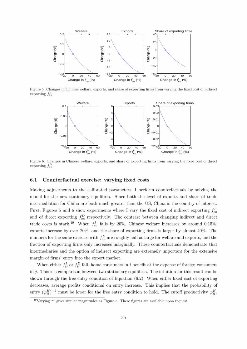
−20 0 20 40 60−0.2

−0.1

0

0.1

0.2

Change in fcuI (%)

Cha

nge

(%)

Welfare

−20 0 20 40 60−15

−10

−5

0

5

10

15

Change in fcuI (%)

Cha

nge

(%)

Exports

−20 0 20 40 60−60

−40

−20

0

20

40

Change in fcuI (%)

Cha

nge

(%)

Share of exporting firms

Figure 5: Changes in Chinese welfare, exports, and share of exporting firms from varying the fixed cost of indirectexporting fIcu.

−20 0 20 40 60−0.1

−0.05

0

0.05

0.1

Change in fcuD (%)

Cha

nge

(%)

Welfare

−20 0 20 40 60−6

−4

−2

0

2

4

6

Change in fcuD (%)

Cha

nge

(%)

Exports

−20 0 20 40 60−0.03

−0.02

−0.01

0

0.01

0.02

0.03

Change in fcuD (%)

Cha

nge

(%)

Share of exporting firms

Figure 6: Changes in Chinese welfare, exports, and share of exporting firms from varying the fixed cost of directexporting fDcu.

6.1 Counterfactual exercise: varying fixed costs

Making adjustments to the calibrated parameters, I perform counterfactuals by solving the

model for the new stationary equilibria. Since both the level of exports and share of trade

intermediation for China are both much greater than the US, China is the country of interest.

First, Figures 5 and 6 show experiments where I vary the fixed cost of indirect exporting f Icu

and of direct exporting fDcu respectively. The contrast between changing indirect and direct

trade costs is stark.49 When f Icu falls by 20%, Chinese welfare increases by around 0.15%,

exports increase by over 20%, and the share of exporting firms is larger by almost 40%. The

numbers for the same exercise with fDcu are roughly half as large for welfare and exports, and the

fraction of exporting firms only increases marginally. These counterfactuals demonstrate that

intermediaries and the option of indirect exporting are extremely important for the extensive

margin of firms’ entry into the export market.

When either f Iij or fDij fall, home consumers in i benefit at the expense of foreign consumers

in j. This is a comparison between two stationary equilibria. The intuition for this result can be

shown through the free entry condition of Equation (6.2). When either fixed cost of exporting

decreases, average profits conditional on entry increase. This implies that the probability of

entry (ϕHii )−k must be lower for the free entry condition to hold. The cutoff productivity ϕHii ,

49Varying τ I gives similar magnitudes as Figure 5. These figures are available upon request.

35

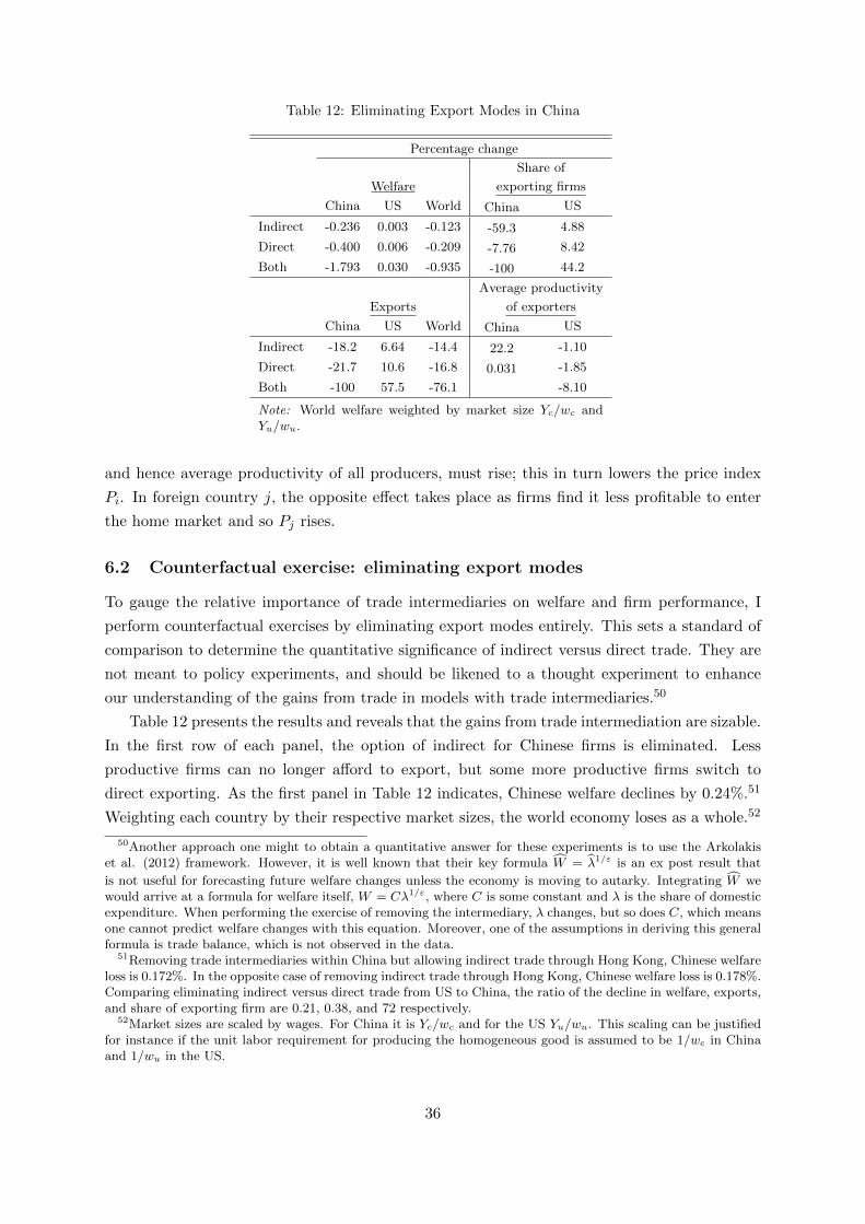
Table 12: Eliminating Export Modes in China

Percentage change

Share of

Welfare exporting firms

China US World China US

Indirect -0.236 0.003 -0.123 -59.3 4.88

Direct -0.400 0.006 -0.209 -7.76 8.42

Both -1.793 0.030 -0.935 -100 44.2

Average productivity

Exports of exporters

China US World China US

Indirect -18.2 6.64 -14.4 22.2 -1.10

Direct -21.7 10.6 -16.8 0.031 -1.85

Both -100 57.5 -76.1 -8.10

Note: World welfare weighted by market size Yc/wc andYu/wu.

and hence average productivity of all producers, must rise; this in turn lowers the price index

Pi. In foreign country j, the opposite effect takes place as firms find it less profitable to enter

the home market and so Pj rises.

6.2 Counterfactual exercise: eliminating export modes

To gauge the relative importance of trade intermediaries on welfare and firm performance, I

perform counterfactual exercises by eliminating export modes entirely. This sets a standard of

comparison to determine the quantitative significance of indirect versus direct trade. They are

not meant to policy experiments, and should be likened to a thought experiment to enhance

our understanding of the gains from trade in models with trade intermediaries.50

Table 12 presents the results and reveals that the gains from trade intermediation are sizable.

In the first row of each panel, the option of indirect for Chinese firms is eliminated. Less

productive firms can no longer afford to export, but some more productive firms switch to

direct exporting. As the first panel in Table 12 indicates, Chinese welfare declines by 0.24%.51

Weighting each country by their respective market sizes, the world economy loses as a whole.52

50Another approach one might to obtain a quantitative answer for these experiments is to use the Arkolakiset al. (2012) framework. However, it is well known that their key formula W = λ1/ε is an ex post result that

is not useful for forecasting future welfare changes unless the economy is moving to autarky. Integrating W wewould arrive at a formula for welfare itself, W = Cλ1/ε, where C is some constant and λ is the share of domesticexpenditure. When performing the exercise of removing the intermediary, λ changes, but so does C, which meansone cannot predict welfare changes with this equation. Moreover, one of the assumptions in deriving this generalformula is trade balance, which is not observed in the data.

51Removing trade intermediaries within China but allowing indirect trade through Hong Kong, Chinese welfareloss is 0.172%. In the opposite case of removing indirect trade through Hong Kong, Chinese welfare loss is 0.178%.Comparing eliminating indirect versus direct trade from US to China, the ratio of the decline in welfare, exports,and share of exporting firm are 0.21, 0.38, and 72 respectively.

52Market sizes are scaled by wages. For China it is Yc/wc and for the US Yu/wu. This scaling can be justifiedfor instance if the unit labor requirement for producing the homogeneous good is assumed to be 1/wc in Chinaand 1/wu in the US.

36

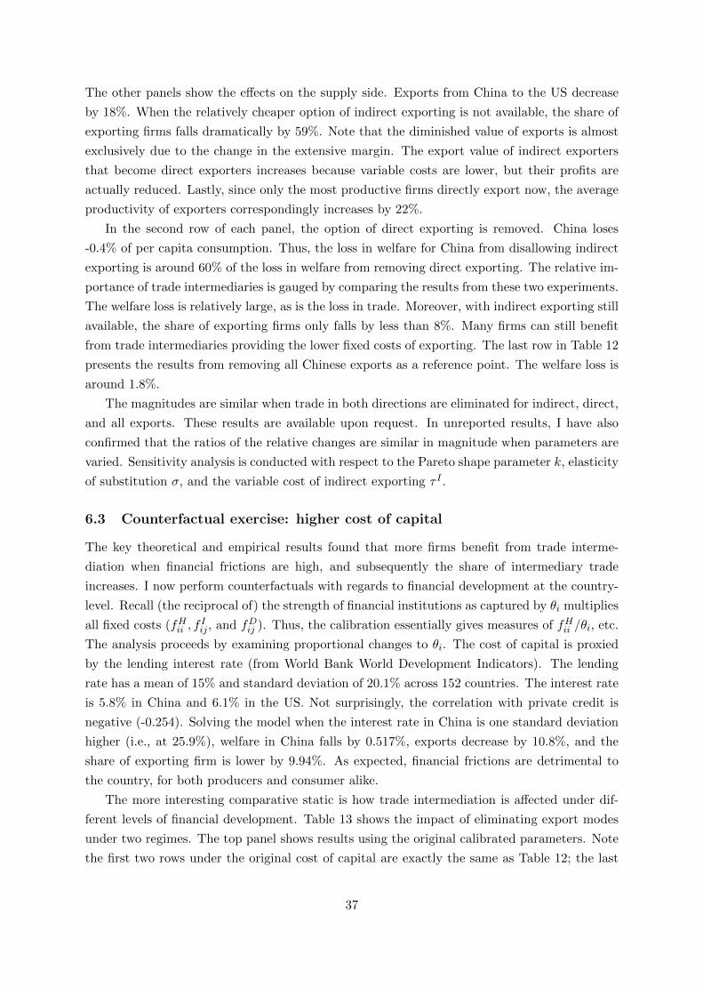
The other panels show the effects on the supply side. Exports from China to the US decrease

by 18%. When the relatively cheaper option of indirect exporting is not available, the share of

exporting firms falls dramatically by 59%. Note that the diminished value of exports is almost

exclusively due to the change in the extensive margin. The export value of indirect exporters

that become direct exporters increases because variable costs are lower, but their profits are

actually reduced. Lastly, since only the most productive firms directly export now, the average

productivity of exporters correspondingly increases by 22%.

In the second row of each panel, the option of direct exporting is removed. China loses

-0.4% of per capita consumption. Thus, the loss in welfare for China from disallowing indirect

exporting is around 60% of the loss in welfare from removing direct exporting. The relative im-

portance of trade intermediaries is gauged by comparing the results from these two experiments.

The welfare loss is relatively large, as is the loss in trade. Moreover, with indirect exporting still

available, the share of exporting firms only falls by less than 8%. Many firms can still benefit

from trade intermediaries providing the lower fixed costs of exporting. The last row in Table 12

presents the results from removing all Chinese exports as a reference point. The welfare loss is

around 1.8%.

The magnitudes are similar when trade in both directions are eliminated for indirect, direct,

and all exports. These results are available upon request. In unreported results, I have also

confirmed that the ratios of the relative changes are similar in magnitude when parameters are

varied. Sensitivity analysis is conducted with respect to the Pareto shape parameter k, elasticity

of substitution σ, and the variable cost of indirect exporting τ I .

6.3 Counterfactual exercise: higher cost of capital

The key theoretical and empirical results found that more firms benefit from trade interme-

diation when financial frictions are high, and subsequently the share of intermediary trade

increases. I now perform counterfactuals with regards to financial development at the country-

level. Recall (the reciprocal of) the strength of financial institutions as captured by θi multiplies

all fixed costs (fHii , fIij , and fDij ). Thus, the calibration essentially gives measures of fHii /θi, etc.

The analysis proceeds by examining proportional changes to θi. The cost of capital is proxied

by the lending interest rate (from World Bank World Development Indicators). The lending

rate has a mean of 15% and standard deviation of 20.1% across 152 countries. The interest rate

is 5.8% in China and 6.1% in the US. Not surprisingly, the correlation with private credit is

negative (-0.254). Solving the model when the interest rate in China is one standard deviation

higher (i.e., at 25.9%), welfare in China falls by 0.517%, exports decrease by 10.8%, and the

share of exporting firm is lower by 9.94%. As expected, financial frictions are detrimental to

the country, for both producers and consumer alike.

The more interesting comparative static is how trade intermediation is affected under dif-

ferent levels of financial development. Table 13 shows the impact of eliminating export modes

under two regimes. The top panel shows results using the original calibrated parameters. Note

the first two rows under the original cost of capital are exactly the same as Table 12; the last

37

Table 13: Outcomes in China

Original cost of capital

Share of

Welfare Exports exporting firms

EliminatingIndirect -0.236 -18.2 -59.3

Direct -0.400 -21.7 -7.76

Ratio of changes (indirect/direct) 0.590 0.836 7.64

1 standard deviation higher

Share of

Welfare Exports exporting firms

EliminatingIndirect -0.213 -17.8 -59.1

Direct -0.362 -21.2 -7.06

Ratio of changes (indirect/direct) 0.589 0.842 8.37

Note: First two rows in each panel in percentage points.

row merely computes the ratio of the two changes for convenience. The bottom panel raises the

cost of capital in China by one standard deviation as explained above, and then performs the

same counterfactual exercises of eliminating export modes. In the bottom panel where the cost

of capital is higher, the magnitudes of the changes in all outcome variables are smaller. This

is to be expected as the overall level of trade has fallen. Since the amount of trade is not the

same under each regime, comparing the levels of each variable can be misleading. Comparison

is instead made between the last row of the two panels to determine the relative importance of

trade intermediation.

First, welfare loss from eliminating indirect exporting relative to direct exporting in China

is larger with lower financial frictions. Since US firms fill the void in the Chinese market left by

Chinese firms, the difference for consumers is very minimal. However, the opposite is true for

producers: trade intermediation is more important for firms when financial frictions increase.

As the last rows in the second and third columns show, total exports fall relatively more when

borrowing costs increase (the ratio is 0.842 versus 0.836). Furthermore, the decline in the share

of exporting firms is relatively greater in the bottom panel. The ratio of relative changes,

8.37 versus 7.64, is almost 10% higher. This calibration exercise provides some corroborating

evidence to the regression analysis, demonstrating the importance of trade intermediaries for

exporters as financial development weakens.

The quantitative exercises presented have compared stationary equilibria and did not in-

corporate any dynamics into the model. Evidence from Bai et al. (2013) suggests that firms

also learn from exporting by selling indirectly through intermediaries. Since the less productive

firms that rely on trade intermediaries to provide them with a cheaper alternative of selling

abroad may realize productivity gains over time, one might expect that the gains from trade

intermediation may be even larger.

38

7 Conclusion

This paper has shown the prevalence of intermediary trade using both firm and country-level

data. Using a model of heterogeneous firms with trade intermediaries and market frictions, I

derive testable implications regarding the characteristics of firms and countries that engage in

indirect exporting. The empirical analysis exploits sectoral variation in financial vulnerability.

Financially more constrained exporting firms are more likely to be indirect exporters, and

correspondingly, in the aggregate, exporting countries with weaker financial institutions have

larger indirect export shares. Both effects are stronger in sectors characterized by high external

finance dependence and low asset tangibility. The role of geography is also critical in determining

indirect export shares through Hong Kong. Institution strength in the contracting environment

is associated with larger indirect export trade as well.

The calibration exercise provides quantitative analysis of the importance of trade interme-

diaries for welfare and global trade. I find that eliminating the option of indirect exporting

leads to a 0.24% welfare loss in China, while removing direct exporting lowers Chinese wel-

fare by 0.40%. There are considerable gains from trade due to the presence of intermediaries.

Exports fall by 18% when trade intermediaries disappear. Moreover, when financial frictions

become larger, the option of indirect exporting is even more valued by firms. When the fixed

costs of production and exporting increase from higher costs of capital, the relative decline in

the share of exporting firms from the elimination of indirect versus direct exporting is 10%

larger. Although the counterfactuals here focus on country-level financial frictions, incorporat-

ing firm-level financial constraints or distortions with intermediary trade will certainly help us

understand quantitatively the role of intermediaries in alleviating credit constraints. This is left

for future research.

The role of trade intermediaries appears to be declining as barriers to trade are being

reduced and information is more readily available and accessible. For entrepot economies like

Hong Kong, they must diversify and find their new comparative advantage. The networks they

have developed over the years are still extremely valuable however, and they must find new ways

to facilitate international trade. Establishments operating in Hong Kong now engage heavily in

offshore trade like merchanting and merchandising for offshore transactions. Research in these

areas will help achieve a more complete understanding of the patterns of global trade.

39

References

Abel-Koch, J. (2013). Who uses intermediaries in international trade? Evidence from firm-levelsurvey data. The World Economy 36 (8), 1041–1064.

Ahn, J., A. K. Khandelwal, and S.-J. Wei (2011). The role of intermediaries in facilitatingtrade. The World Economy 84 (1), 7385.

Akerman, A. (2014). A theory on the role of wholesalers in international trade based oneconomies of scope. Stockholm University mimeo.

Anderson, J. E. and E. van Wincoop (2004). Trade costs. Journal of Economic Literature 42 (3),691–751.

Andriamananjara, S., H. Arce, and M. J. Ferrantino (2004). Transshipment in the UnitedStates. U.S. International Trade Commission Office of Economics Working Paper .

Antras, P. and A. Costinot (2010). Intermediated trade. Quarterly Journal of Eco-nomics 126 (3), 1319–1374.

Arkolakis, C., A. Costinot, and A. Rodrıguez-Clare (2012). New trade models, same old gains?American Economic Review 102 (1), 94–130.

Aterido, R., M. Hallward-Driemeier, and C. Pages (2011). Big constraints to small firms’growth: Business environment and employment growth across firms. Economic Developmentand Cultural Change 59 (3), 609–647.

Bai, X., K. Krishna, and H. Ma (2013). How you export matters: Export mode, learning andproductivity in China. Pennsylvania State University Mimeo.

Bartelsman, E., J. Haltiwanger, and S. Scarpetta (2013). Cross-country differences in produc-tivity: The role of allocation and selection. American Economic Review 103 (1), 305–334.

Beck, T. (2002). Financial development and international trade: is there a link? Journal ofInternational Economics 57 (1), 107–131.

Beck, T. (2003). Financial dependence and international trade. Review of International Eco-nomics 11, 296–316.

Beck, T., A. Demirguc-Kunt, and R. Levine (2000). A new database on the structure anddevelopment of the financial sector. World Bank Economic Review 14 (3), 597–605.

Becker, B., J. Chen, and D. Greenberg (2013). Financial development, fixed costs, and inter-national trade. Review of Corporate Finance Studies 2 (1), 1–28.

Berman, N. and J. Hericourt (2010). Financial factors and the margins of trade: Evidence fromcross-country firm-level data. Journal of Development Economics 93 (2), 206–217.

Bernard, A. B., E. J. Blanchard, I. V. Beveren, and H. Vandenbussche (2012). Carry-alongtrade. NBER Working Paper No. 18246 .

Bernard, A. B., M. Grazzi, and C. Tomasi (2013). Intermediaries in international trade: Marginsof trade and export flows. NBER Working Papers No. 17711 .

Bernard, A. B., J. B. Jensen, S. J. Redding, and P. K. Schott (2010). Wholesalers and retailersin US trade. American Economic Review 100 (2), 408–413.

40

Blum, B. S., S. Claro, and I. Horstmann (2010). Facts and figures on intermediated trade.American Economic Review 100 (2), 419–423.

Blum, B. S., S. Claro, and I. Horstmann (2011). Intermediation and the nature of trade costs:Theory and evidence. University of Toronto Mimeo.

Braun, M. (2003). Financial contractibtility and asset hardness. University of California- LosAngeles mimeo.

Breinlich, H. and A. Cunat (2011). Trade liberalization and heterogeneous firm models: Anevaluation using the Canada - US Free Trade Agreement. LSE and University of EssexMimeo.

Broda, C. and D. E. Weinstein (2006). Globalization and the gains from variety. QuarterlyJournal of Economics 121 (2), 541–585.

Castro, L., B. Li, K. E. Maskus, and Y. Xie (2014). Fixed export costs and export behavior.CESifo Working Paper No. 4697 .

Central Bank of the Republic of China (Taiwan) (2013). Financial Statistics. http://www.cbc.gov.tw/content.asp?mp=2&CuItem=2069. Accessed: 15/12/2013.

Chamberlain, G. (1980). Analysis of variance with qualitative data. Review of EconomicStudies 47, 225238.

Chan, J. M. and K. Manova (2014). Financial development and the choice of trade partners.NBER Working Paper No. 18867 .

Chaney, T. (2013). Liquidity constrained exporters. NBER Working Paper No. 19170 .

Claessens, S. and L. Laeven (2003). Financial development, property rights, and growth. Journalof Finance 58 (6), 2401–2436.

Crozet, M., G. Lalanne, and S. Poncet (2013). Wholesalers in international trade. EuropeanEconomic Review 58, 1–17.

Das, S., M. J. Roberts, and J. R. Tybout (2007). Market entry costs, producer heterogeneity,and export dynamics. Econometrica 75 (3), 837–873.

de Vries, G. J. (2014). Productivity in a distorted market: The case of Brazil’s retail sector.Review of Income and Wealth 60 (3), 499–524.

Demir, B. and B. Javorcik (2014). Grin and bear it: Producer-financed exports from an emergingmarket. University of Oxford Mimeo.

Eckel, C. and R. Riezman (2013). Cats and dogs. University of Iowa Mimeo.

Ellis, P. (2003). Are international trade intermediaries catalysts in economic development? Anew research agenda. Journal of International Marketing 11 (1), 73–93.

Feenstra, R. C. and G. H. Hanson (2004). Intermediaries in entrepot trade: Hong Kong re-exports of Chinese goods. Journal of Economics and Management Strategy 13 (1), 335.

Felbermayr, G. and B. Jung (2011). Trade intermediation and the organization of exporters.Review of International Economics 19 (4), 634–648.

41

Fisman, R., P. Moustakerski, and S.-J. Wei (2008). Outsourcing tariff evasion: A new explana-tion for entrepot trade. Review of Economics and Statistics 90 (3), 587–592.

Fisman, R. and Svensson (2007). Are corruption and taxation really harmful to growth? Firmlevel evidence. Journal of Development Economics 83, 63–75.

Fryges, H. (2007). The change of sales modes in international markets: Empirical results forGerman and British high-tech firms. Progress in International Business Research 1, 139–185.

Head, K., T. Mayer, and M. Thoenig (2014). Welfare and trade without Pareto. AmericanEconomic Review: Papers & Proceedings 104 (5), 310–316.

Helpman, E., M. J. Melitz, and Y. Rubinstein (2008). Estimating trade flows: Trading partnersand trading volumes. Quarterly Journal of Economics 123 (2), 441–487.

Helpman, E., M. J. Melitz, and S. R. Yeaple (2004). Export versus FDI with heterogeneousfirms. American Economic Review .

Hessels, J. and S. Terjesen (2010). Resource dependency and institutional theory perspectiveson direct and indirect export choices. Small Business Economics 34 (2), 203–220.

Hoefele, A., T. Schmidt-Eisenlohr, and Z. Yu (2013). Payment choice in international trade:Theory and evidence from cross-country firm level data. CESifo Working Paper No. 4350 .

Hong Kong Census and Statistics Department (2013a). Hong Kong merchandise trade statisticsimports. http://www.censtatd.gov.hk/hkstat/sub/sp230.jsp?productCode=B1020001.Accessed: 15/12/2013.

Hong Kong Census and Statistics Department (2013b). How to complete and lodge im-port/export declarations. www.censtatd.gov.hk/FileManager/EN/Content_93/B8XX0022.

pdf. Accessed: 15/12/2013.

Hong Kong Trade Development Council (2012). Import and Export Trade Industry in HongKong . http://hong-kong-economy-research.hktdc.com/business-news/article/

Hong-Kong-Industry-Profiles/Import-and-Export-Trade-Industry-in-Hong-Kong/

hkip/en/1/1X000000/1X006NJK.htm. Accessed: 03/09/2014.

Hsieh, C.-T. and P. J. Klenow (2009). Misallocation and manufacturing TFP in China andIndia. Quarterly Journal of Economics 124 (4), 1403–1448.

Hur, J., M. Raj, and Y. E. Riyanto (2006). Finance and trade: A cross-country empiricalanalysis on the impact of financial development and asset tangibility on international trade.World Development 34 (10), 1728–1741.

Keller, W., B. Li, and C. H. Shiue (2011). China’s foreign trade: Perspectives from the past150 years. The World Economy 34 (6), 853–892.

KPMG International (2013). Corporate and Indirect Tax Survey 2012. http:

//www.kpmg.com/Global/en/IssuesAndInsights/ArticlesPublications/Documents/

corporate-and-indirect-tax-rate-survey-2011.pdf. Accessed: 15/12/2013.

Krishna, K. and Y. Sheveleva (2013). Wheat or strawberries? Intermediated trade with limitedcontracting. Pennsylvania State University Mimeo.

42

Lu, J., Y. Lu, and Z. Tao (2011). Intermediaries, firm heterogeneity, and exporting behavior.Peking University Mimeo.

Manova, K. (2008). Credit constraints, equity market liberalizations and international trade.Journal of International Economics 76, 33–47.

Manova, K. (2013). Credit constraints, heterogeneous firms, and international trade. Review ofEconomic Studies 80, 711–744.

Mayer, T. and S. Zignago (2011). Notes on CEPIIs distances measures (Geodist). CEPIIWorking Paper 2011-25 .

McCann, F. (2013). Indirect exporters. Journal of Industry, Competition and Trade 13 (4),519–535.

Melitz, M. (2003). The impact of trade on intra-industry reallocations and aggregate industryproductivity. Econometrica 71, 1695–1725.

Melitz, M. J. and S. J. Redding (2013). New trade models, new welfare implications. NBERWorking Papers No. 18919 .

Minetti, R. and S. C. Zhu (2011). Credit constraints and firm export: Microeconomic evidencefrom Italy. Journal of International Economics 83, 109125.

Mundlak, Y. (1980). On the pooling of time series and cross section data. Econometrica 46 (1),69–85.

Muuls, M. (2008). Exporters and credit constraints. A firm-level approach. National Bank ofBelgium Working Paper Research 139 .

Nunn, N. and D. Trefler (2013a). Domestic institutions as a source of comparative advantage.NBER Working Paper No. 18851 .

Nunn, N. and D. Trefler (2013b). Incomplete contracts and the boundaries of the multinationalfirm. Journal of Economic Behavior & Organization 94, 330–344.

Olney, W. W. (2014). Impact of corruption on firm level export decisions. Williams Collegemimeo.

Papke, L. E. and J. M. Wooldridge (2008). Panel data methods for fractional response variableswith an application to test pass rates. Journal of Econometrics 145 (1-2), 121–133.

Petropoulou, D. (2011). Information costs, networks and intermediation in international trade.Federal Reserve Bank of Dallas Globalization and Monetary Policy Institute Working PaperNo. 76 .

Rajan, R. G. and L. Zingales (1998). Financial dependence and growth. American EconomicReview 88 (3), 559–586.

Svaleryd, H. and J. Vlachos (2005). Financial markets, the pattern of industrial specializa-tion and comparative advantage: Evidence from OECD countries. European Economic Re-view 49 (1), 113–144.

Tang, H. and Y. Zhang (2012). Quality differentiation and trade intermediation. Tufts UniversityMimeo.

43

Wooldridge, J. M. (2002). Econometric Analysis of Cross Section and Panel Data. Cambridge,MA: MIT Press.

World Bank (2014). Survey Methodology. http://www.enterprisesurveys.org/

methodology. Accessed: 03/09/2014.

Young, A. (1999). Transport, processing and information: Value added and the circuitousmovement of goods. University of Chicago mimeo.

44

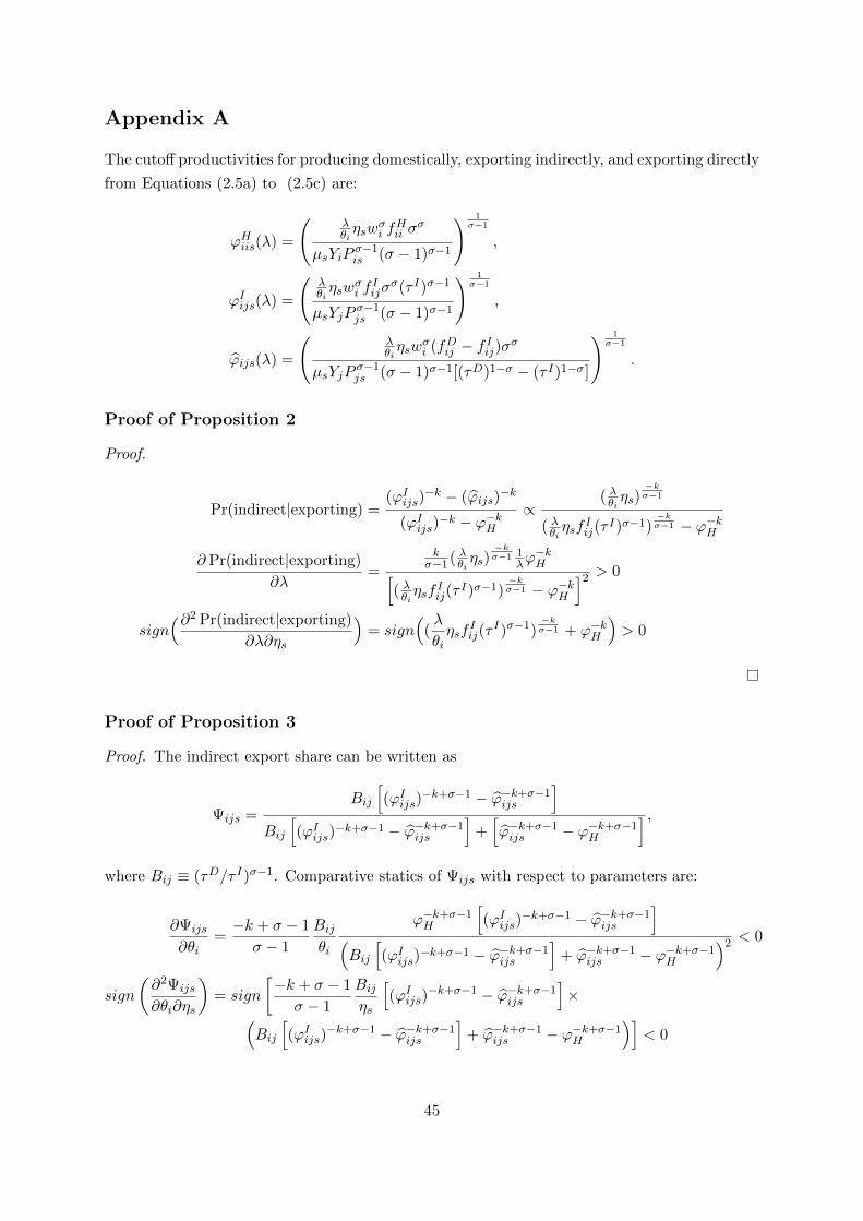
Appendix A

The cutoff productivities for producing domestically, exporting indirectly, and exporting directly

from Equations (2.5a) to (2.5c) are:

ϕHiis(λ) =

(λθiηsw

σi f

Hii σ

σ

µsYiPσ−1is (σ − 1)σ−1

) 1σ−1

,

ϕIijs(λ) =

(λθiηsw

σi f

Iijσ

σ(τ I)σ−1

µsYjPσ−1js (σ − 1)σ−1

) 1σ−1

,

ϕijs(λ) =

(λθiηsw

σi (fDij − f Iij)σσ

µsYjPσ−1js (σ − 1)σ−1[(τD)1−σ − (τ I)1−σ]

) 1σ−1

.

Proof of Proposition 2

Proof.

Pr(indirect|exporting) =(ϕIijs)

−k − (ϕijs)−k

(ϕIijs)−k − ϕ−kH

∝( λθi ηs)

−kσ−1

( λθi ηsfIij(τ

I)σ−1)−kσ−1 − ϕ−kH

∂ Pr(indirect|exporting)

∂λ=

kσ−1( λθi ηs)

−kσ−1 1

λϕ−kH[

( λθi ηsfIij(τ

I)σ−1)−kσ−1 − ϕ−kH

]2 > 0

sign(∂2 Pr(indirect|exporting)

∂λ∂ηs

)= sign

((λ

θiηsf

Iij(τ

I)σ−1)−kσ−1 + ϕ−kH

)> 0

Proof of Proposition 3

Proof. The indirect export share can be written as

Ψijs =Bij

[(ϕIijs)

−k+σ−1 − ϕ−k+σ−1ijs

]Bij

[(ϕIijs)

−k+σ−1 − ϕ−k+σ−1ijs

]+[ϕ−k+σ−1ijs − ϕ−k+σ−1

H

] ,where Bij ≡ (τD/τ I)σ−1. Comparative statics of Ψijs with respect to parameters are:

∂Ψijs

∂θi=−k + σ − 1

σ − 1

Bijθi

ϕ−k+σ−1H

[(ϕIijs)

−k+σ−1 − ϕ−k+σ−1ijs

](Bij

[(ϕIijs)

−k+σ−1 − ϕ−k+σ−1ijs

]+ ϕ−k+σ−1

ijs − ϕ−k+σ−1H

)2 < 0

sign

(∂2Ψijs

∂θi∂ηs

)= sign

[−k + σ − 1

σ − 1

Bijηs

[(ϕIijs)

−k+σ−1 − ϕ−k+σ−1ijs

]×(

Bij

[(ϕIijs)

−k+σ−1 − ϕ−k+σ−1ijs

]+ ϕ−k+σ−1

ijs − ϕ−k+σ−1H

)]< 0

45

We also have:

sign

(∂Ψijs

∂Yj

)= sign

(−k + σ − 1

σ − 1

BijYj

ϕ−k+σ−1H

[(ϕIijs)

−k+σ−1 − ϕ−k+σ−1ijs

])< 0

sign

(∂Ψijs

∂τD

)= sign

(Bij

[σ − 1

τD

((ϕIijs)

−k+σ−1 − ϕ−k+σ−1ijs

)(ϕ−k+σ−1ijs − ϕ−k+σ−1

H

)−

(−k + σ − 1)ϕ−k+σ−1ijs (τD)−σ

(τD)1−σ − (τ I)1−σ

((ϕIijs)

−k+σ−1 − ϕ−k+σ−1H

)])> 0

sign

(∂Ψijs

∂τ I

)= sign

(Bij

[−σ − 1

τ I

((ϕIijs)

−k+σ−1 − ϕ−k+σ−1ijs

)+

(−k + σ − 1)ϕ−k+σ−1ijs (τ I)−σ

(τD)1−σ − (τ I)1−σ

((ϕIijs)

−k+σ−1 − ϕ−k+σ−1H

)])< 0

sign

(∂Ψijs

∂fDij

)= sign

(k − σ + 1

σ − 1

Bij

fDij − f Iijϕ−k+σ−1ijs

[(ϕIijs)

−k+σ−1 − ϕ−k+σ−1H

])> 0

Appendix B

Countries in World Bank Enterprise Surveys Dataset

Africa: Angola, Benin, Botswana, Burkina Faso, Burundi, Cameroon, Cape Verde, Central

African Republic, Chad, Democratic Republic of Congo, Republic of Congo, Eritrea, Ethiopia,

Gabon, Gambia, Ghana, Guinea, Guinea Bissau, Ivory Coast, Kenya, Lesotho, Liberia, Mada-

gascar, Malawi, Mali, Mauritania, Mauritius, Mozambique, Namibia, Niger, Nigeria, Rwanda,

Senegal, Sierra Leone, South Africa, Swaziland, Tanzania, Togo, Uganda, Zambia, Zimbabwe

East Asia Pacific: Fiji, Indonesia, Lao People’s Democratic Republic, Micronesia, Philippines,

Samoa, Timor Leste, Tonga, Vanuatu, Vietnam

Europe Central Asia: Albania, Armenia, Azerbaijan, Belarus, Bosnia and Herzegovina,

Bulgaria, Croatia, Czech Republic, Estonia, Georgia, Hungary, Kazakhstan, Kosovo, Kyrgyz

Republic, Latvia, Lithuania, Macedonia, Moldova, Mongolia, Montenegro, Poland, Romania,

Russian Federation, Serbia, Slovak Republic, Slovenia, Tajikistan, Turkey, Ukraine, Uzbekistan

Latin America and Caribbean: Antigua and Barbuda, Argentina, Bahamas, Barbados,

Belize, Bolivia, Brazil, Chile, Colombia, Costa Rica, Dominica, Dominican Republic, Ecuador,

El Salvador, Grenada, Guatemala, Guyana, Honduras, Jamaica, Mexico, Nicaragua, Panama,

Paraguay, Peru, St. Kitts and Nevis, St. Lucia, St. Vincent and the Grenadines, Suriname,

Trinidad and Tobago, Uruguay, Venezuela

South Asia Region: Afghanistan, Bangladesh, Bhutan, Nepal, Pakistan, Sri Lanka

Other: China, Iraq, Yemen

46

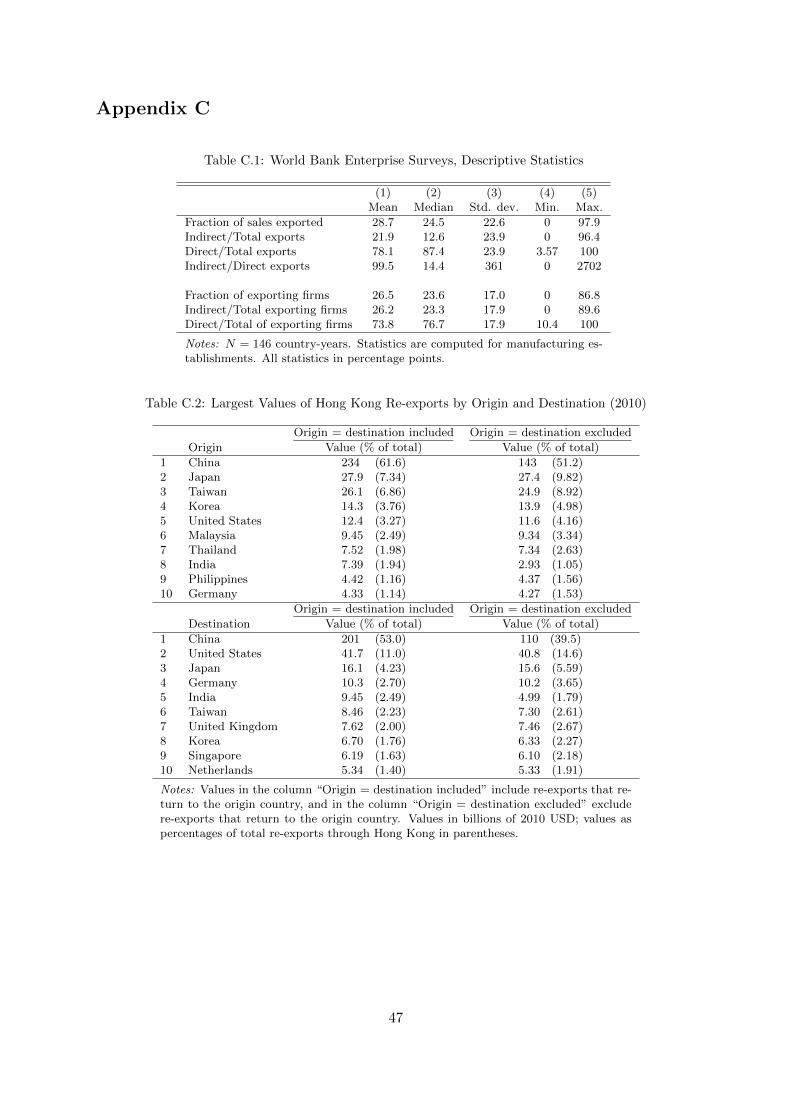
Appendix C

Table C.1: World Bank Enterprise Surveys, Descriptive Statistics

(1) (2) (3) (4) (5)Mean Median Std. dev. Min. Max.

Fraction of sales exported 28.7 24.5 22.6 0 97.9Indirect/Total exports 21.9 12.6 23.9 0 96.4Direct/Total exports 78.1 87.4 23.9 3.57 100Indirect/Direct exports 99.5 14.4 361 0 2702

Fraction of exporting firms 26.5 23.6 17.0 0 86.8Indirect/Total exporting firms 26.2 23.3 17.9 0 89.6Direct/Total of exporting firms 73.8 76.7 17.9 10.4 100

Notes: N = 146 country-years. Statistics are computed for manufacturing es-tablishments. All statistics in percentage points.

Table C.2: Largest Values of Hong Kong Re-exports by Origin and Destination (2010)

Origin = destination included Origin = destination excluded

Origin Value (% of total) Value (% of total)

1 China 234 (61.6) 143 (51.2)2 Japan 27.9 (7.34) 27.4 (9.82)3 Taiwan 26.1 (6.86) 24.9 (8.92)4 Korea 14.3 (3.76) 13.9 (4.98)5 United States 12.4 (3.27) 11.6 (4.16)6 Malaysia 9.45 (2.49) 9.34 (3.34)7 Thailand 7.52 (1.98) 7.34 (2.63)8 India 7.39 (1.94) 2.93 (1.05)9 Philippines 4.42 (1.16) 4.37 (1.56)10 Germany 4.33 (1.14) 4.27 (1.53)

Origin = destination included Origin = destination excluded

Destination Value (% of total) Value (% of total)

1 China 201 (53.0) 110 (39.5)2 United States 41.7 (11.0) 40.8 (14.6)3 Japan 16.1 (4.23) 15.6 (5.59)4 Germany 10.3 (2.70) 10.2 (3.65)5 India 9.45 (2.49) 4.99 (1.79)6 Taiwan 8.46 (2.23) 7.30 (2.61)7 United Kingdom 7.62 (2.00) 7.46 (2.67)8 Korea 6.70 (1.76) 6.33 (2.27)9 Singapore 6.19 (1.63) 6.10 (2.18)10 Netherlands 5.34 (1.40) 5.33 (1.91)

Notes: Values in the column “Origin = destination included” include re-exports that re-turn to the origin country, and in the column “Origin = destination excluded” excludere-exports that return to the origin country. Values in billions of 2010 USD; values aspercentages of total re-exports through Hong Kong in parentheses.

47

Table C.3: Composition of Hong Kong Re-exports (2010)

Destination Region Origin RegionCountry Chn Asia Eur. Am. Afr. Chn Asia Eur. Am. Afr.

China 37.1 29.4 32.0 1.46 77.0 11.3 10.7 0.97Japan 86.7 8.28 2.42 2.41 0.16 92.7 3.76 2.12 1.27 0.14India 43.0 31.6 13.7 11.7 0.14 81.7 8.37 5.56 2.18 2.13Australia 74.5 22.3 2.00 1.03 0.18 75.4 5.28 17.9 1.37 0.09Israel 31.8 16.1 7.53 44.6 0.01 78.0 16.8 2.59 0.78 1.85Germany 80.2 18.1 0.71 0.87 0.11 93.3 4.52 0.45 1.65 0.05United States 74.3 22.2 3.29 0.17 0.07 92.2 6.19 1.12 0.26 0.19Nigeria 88.7 9.12 2.22 0.01 0 90.5 8.33 0.93 0.16 <0.01

Notes: Rows in each panel sum to 100%. Abbreviations: Chn- China, Asia- Asia exclud-ing China, Eur.- Europe, Am.- Americas, and Afr.- Africa. In both panels, observationswhere the origin is the same as the destination are excluded.

Table C.4: Re-export Shares by Destination and Origin Regions (2010)

Destination Region Origin RegionCountry Chn Asia Eur. Am. Afr. Chn Asia Eur. Am. Afr.

China 8.57 9.82 9.98 2.52 9.82 6.23 5.50 4.58Japan 12.7 0.74 0.63 0.38 0.42 10.1 0.20 0.43 0.21 0.24India 6.76 1.28 1.09 1.15 0.03 8.86 0.37 0.52 0.36 0.62Australia 0.88 0.13 0.07 0.06 0.01 9.91 0.36 2.18 0.23 0.17Israel 23.4 2.57 0.69 3.10 0.01 9.53 0.81 0.09 0.04 1.05Germany 4.46 0.51 <0.01 0.02 0.02 11.8 0.31 0.01 0.23 0.02United States 8.19 0.81 0.14 <0.01 0.03 11.4 0.61 0.13 0.01 0.16Nigeria 1.03 0.01 <0.01 <0.01 0 1.27 0.29 0.02 0.01 <0.01

Notes: Abbreviations: Chn- China, Asia- Asia excluding China, Eur.- Europe, Am.- Amer-icas, and Afr.- Africa. In both panels, observations where the origin is the same as the des-tination are excluded. Total re-exports and direct exports are first separately aggregatedby region, then the re-export share for each region is calculated.

01

23

45

(log)

Rea

l Re−

Exp

orts

(bill

ions

of 2

005

US

D)

2002 2004 2006 2008 2010 2012Year

China Asia excl. China EuropeAmericas Africa

By Origin Region

(a)

01

23

45

(log)

Rea

l Re−

Exp

orts

(bill

ions

of 2

005

US

D)

2002 2004 2006 2008 2010 2012Year

China Asia excl. China EuropeAmericas Africa

By Destination Region

(b)

Figure C.1: (a) (log) Real Hong Kong re-exports by origin region; (b) (log) Real Hong Kong re-exports bydestination region. Observations where the origin is the same as the destination are excluded.

48

05

1015

2025

Re−

expo

rt S

hare

s

2002 2004 2006 2008 2010 2012Year

China Asia excl. China EuropeAmericas Africa

By Origin Region

(a)

05

1015

2025

Re−

expo

rt S

hare

s

2002 2004 2006 2008 2010 2012Year

China Asia excl. China EuropeAmericas Africa

By Destination Region

(b)

Figure C.2: (a) Re-export shares through Hong Kong by origin region; (b) Re-export shares through Hong Kongby destination region. Observations where the origin is the same as the destination are excluded.

49

Appendix D

Note Mi = M ei (ϕHii )−k and τ I = τD = τ . The following equations can be derived for i = c, u:

wifHii =

k − σ + 1

σk

µYi −Xji

Mi

f Iij =

1

Xij

σk

k − σ + 1τ−kwi

(wiwj

)− σkσ−1 Mj

M ej

M ei

(XIij

XDij

+ 1

)(XIij

γXDij

+ γ−σ

)−1

fHjj

σ−1k−σ+1

fHjj

fDij =

( XIij

γXDij

+ γ−σ

) σ−1k−σ+1

(1− γ−σ)γσk

k−σ+1 + 1

f IijM ei =

σ − 1

σk

µYi +XIij/γ +XD

ij −Xji

wifEii

The calibration will also use the following equation:

M eu =

(1

XDcu

) kσ−1

(σk

k − σ + 1

) kσ−1

τ−kw−kc Mk

σ−1c Mu

(Mc

Mc

) k−σ+1σ−1 M e

c

Mcw

σkσ−1u (fHuu)

kσ−1 ,

where McMc

is the fraction of directly exporting firms in China.

50