travaux mathématiques - urząd miasta...
TRANSCRIPT
Travaux mathématiques
Faculty of Science,Technology
and Communication
Travaux mathématiques
Presentation The journal « Travaux mathématiques » is published by the Mathematics Seminar of the University of Luxembourg. Even though the main focus of the journal is on original research articles, surveys and historical studies are also welcome.
Editors-in-Chief
Carine Molitor-Braun (University of Luxembourg)Norbert Poncin (University of Luxembourg)
Address: University of Luxembourg Avenue de la Faïencerie, 162AL-1511 Luxembourg CityGrand-Duchy of LuxembourgEmail: [email protected] or [email protected] [email protected]
Associate Editors
Jean Ludwig (University Paul Verlaine, Metz – University of Luxembourg)Martin Olbrich (University of Luxembourg)Martin Schlichenmaier (University of Luxembourg)Anton Thalmaier (University of Luxembourg)
Editorial Board
Bachir Bekka (University of Rennes)Lionel Bérard-Bergery (University H. Poincaré, Nancy)Martin Bordemann (University of Haute Alsace, Mulhouse)Johannes Huebschmann (University of Lille)Pierre Lecomte (University of Liège)Jiang-Hua Lu (University of Hong Kong)Raymond Mortini (University Paul Verlaine, Metz)Jean-Paul Pier (University of Luxembourg)Claude Roger (University Claude Bernard, Lyon) Izu Vaisman (University of Haifa)Alain Valette (University of Neuchâtel)Robert Wolak (Jagiellonian University of Krakow)
Travaux mathématiques
–Special Issue: Proceedings of the 8th Conference on
Geometry and Topology of Manifolds–
Editors:Jan Kubarski
Norbert PoncinRobert Wolak
_
Volume XVIII, 2008
Faculty of Science,Technology
and Communication

Proceedings1 of the 8th Conference on
Geometry and Topology of Manifolds
(Lie algebroids, dynamical systems and applications)
Luxembourg-Poland-Ukraine conference
Przemysl (Poland) - L’viv (Ukraine) 30.04.07 - 6.05.2007
Edited by
Norbert PoncinJan KubarskiRobert Wolak
1Additionally including two regular papers submitted to “Travaux Mathematiques”.
2
The Organizing Committee
Jan Kubarski, chairman, ÃLodz, Poland, email: [email protected]– Institute of Mathematics of the Technical University of Lodz, ÃLodz
Robert Wolak, Krakow, Poland, email: [email protected]– Institute of Mathematics of the Jagiellonian University, Krakow
Tomasz Rybicki, Krakow, Poland, email: [email protected]– Institute of Mathematics of the Jagiellonian University, Krakow
Michael Zarichny, Rzeszow, Poland; L’viv, Ukraine, email: [email protected]– Institute of Mathematics, Rzeszow University, Rzeszow– Faculty of Mechanics and Mathematics of L’viv Ivan Franko National Univer-sity, L’viv
Norbert Poncin, Luxembourg, Luxembourg, email: [email protected]– Institute of Mathematics, University of Luxembourg, Grand-Duchy of Luxem-bourg
Andriy Panasyuk, Warsaw, Poland; L’viv, Ukraine, email: [email protected]– Institute for Applied Problems of Mechanics and Mathematics of NationalAcademy of Sciences of Ukraine, L’viv– Department of Mathematical Methods in Physics, University of Warsaw, War-saw
Vladimir Sharko, Kiev, Ukraine, email: [email protected]– Institute of Mathematics of the National Academy of Sciences of Ukraine, Kiev
The Scientific Committee
Yu. Aminow (Ukraine) V. Yu. Ovsienko (France)B. Bojarski (Poland) J. Pradines (France)A. Borisenko (Ukraine) A. O. Prishlyak (Ukraine)R. Brown (UK) A. M. Samoilenko (Ukraine)S. Brzychczy (Poland) V. Sharko (Ukraine)J. Grabowski (Poland) N. Teleman (Italy)J. Kubarski (Poland) M. Zarichny (Poland, Ukraine)P. Lecomte (Belgium) N. T. Zhung (France)A. S. Mishchenko (Russia)
3
The Sponsors
Committee on Mathematics of the Polish Academy of SciencesTechnical University of LodzJagiellonian UniversityAGH University of Science and TechnologyRzeszow UniversityUniversity of WarsawUniversity of LuxembourgL’viv Ivan Franko National UniversityNational Academy of Sciences of UkraineBank“Dnister”, L’viv“Kredo Bank”, L’viv

5
Foreword
This eighth conference of a cycle, which was initiated in 1998 with a meeting inKonopnica (see http://im0.p.lodz.pl/konferencje/), took place in two cities;the first part was held in Przemysl, Poland, at the State High School of EastEurope, the second part in L’viv, Ukraine, at the Ivan Franko National Universityof L’viv.
The main aim of the conference series is to present and discuss new results ongeometry and topology of manifolds with particular attention paid to applicationsof algebraic methods. The topics that are usually discussed include:
• Dynamical systems on manifolds and applications
• Lie groups (including infinite dimensional ones), Lie algebroids and theirgeneralizations, Lie groupoids
• Characteristic classes, index theory, K-theory, Fredholm operators
• Singular foliations, cohomology theories for foliated manifolds and their quo-tients
• Symplectic, Poisson, Jacobi and special Riemannian manifolds
• Topology of infinite-dimensional manifolds
• Applications to mathematical physics
Jan Kubarski
Robert Wolak

7
List of Participants
1. Abe, Kojun, Shinshu University, Matsumoto, Nagano Prefecture, Japan
2. Aminov, Yuriy, National Academy of Sciences of Ukraine, Kharkiv, Ukraine
3. Ammar, Mourad, University of Luxembourg, Luxembourg, Grand-Duchy ofLuxembourg
4. Balcerzak, Bogdan, Technical University of Lodz, ÃLodz, Poland
5. Banakh, Taras, National University, L’viv, Ukraine
6. Bazylevych, Lidia, National University, L’viv, Ukraine
7. Bojarski, Bogdan, Polish Academy of Sciences, Warszawa, Poland
8. Bokalo, Bogdan, L’viv Ivan Franko National University, L’viv, Ukraine
9. Casati, Paolo, II Universita di Milano, Milano, Italy
10. Eichhorn, Juergen, Greifswald University, Greifswald, Germany
11. Fregier, Yael, University of Luxembourg, Luxembourg, Grand-Duchy ofLuxembourg
12. Grabowska, Katarzyna, University of Warsaw, Warsaw, Poland
13. Grabowski, Janusz, Polish Academy of Sciences, Warsaw, Poland
14. Gutik, Oleg, L’viv Ivan Franko National University, L’viv, Ukraine
15. Hajduk, BogusÃlaw, University of WrocÃlaw, WrocÃlaw, Poland
16. Hall, Graham, University of Aberdeen, Aberdeen, UK
17. Hausmann, Jean-Claude, Universite de Geneve, Geneve, Switzerland
18. Hryniv, Olena, L’viv Ivan Franko National University, L’viv, Ukraine
19. Jaworowski, Jan, Bloomingon, Indiana, USA
20. Jozefowicz, MaÃlgorzata, Jagiellonian University, Cracow, Poland
21. Kass, Guy, University of Luxembourg, Luxembourg, Grand-Duchy of Lux-embourg
22. Kotov, Alexei, University of Luxembourg, Luxembourg, Grand-Duchy ofLuxembourg
23. Kowalik, Agnieszka, AGH University of Science and Technology, Cracow,Poland
24. Krantz, Thomas, University of Luxembourg, Luxembourg, Grand-Duchy ofLuxembourg
25. Kravchuk, Olga, The Khmelnytskyi National University, Khmelnytskyi, Ukraine
26. Krot-Sieniawska, Ewa, University of Bialystok, BiaÃlystok, Poland
27. Kubarski, Jan, Technical University of Lodz, ÃLodz, Poland
28. Kwasniewski, Andrzej Krzysztof, University of Bialystok, BiaÃlystok, Poland
29. Leandre, Remi, Universite de Bourgogne, Dijon, France
8
30. Lech, Jacek, AGH University of Science and Technology, Cracow, Poland
31. Lyaskovska Nadya, L’viv Ivan Franko National University, L’viv, Ukraine
32. Maakestad, Helge, The Norwegian University of Science and Technology(NTNU), Trondheim, Norway
33. Maksymenko, Sergiy, National Academy of Sciences of Ukraine, Kyiv, Ukraine
34. Matsyuk, Roman, National Academy of Sciences of Ukraine, L’viv, Ukraine
35. Mazurenko, Nataliia, Pre-Carpathian National University of Ukraine, Ivano-Frankivsk, Ukraine
36. Michalik, Ilona, AGH University of Science and Technology, Cracow, Poland
37. Mormul, Piotr, Warsaw University, Warsaw, Poland
38. Muranov, Yury Vladimirovich, Vitebsk State University, Vitebsk, Belarus
39. Mykytyuk, Ihor, Rzeszow State University, Rzeszow, Poland
40. Nguiffo Boyom, Michel, University Montpellier, Montpellier, France
41. Ovsienko, Valentin, University Claude Bernard Lyon 1, Lyon, France
42. Panasyuk, Andriy, University of Warsaw, Warsaw, Poland; National Academyof Sciences of Ukraine, L’viv, Ukraine
43. Pavlov, Alexander, Moscow State University, Moscow, Russia
44. Pelykh, Wolodymyr, National Academy of Sciences of Ukraine, L’viv, Ukraine
45. Petrenko, O., Kyiv National University, Kyiv, Ukraine
46. Poncin, Norbert, University of Luxembourg, Luxembourg, Grand-Duchy ofLuxembourg
47. Popescu, Paul, University of Craiova, Craiova, Romania
48. Pradines, Jean, Universite Toulouse III, Toulouse, France
49. Protasov, Igor, Kyiv National University, Kyiv, Ukraine
50. Pyrch, Nazar, Ukrainian Academy of Printing, L’viv, Ukraine
51. Radoux, Fabian, University of Luxembourg, Luxembourg, Grand-Duchy ofLuxembourg
52. Rodrigues, Alexandre, University of Sao Paulo, Sao Paulo, Bazil
53. Rotkiewicz, MikoÃlaj, Warsaw University, Warsaw, Poland
54. Rubin, Matatyahu, Ben Gurion University, Beer Sheva, Israel
55. Rybicki, Tomasz, AGH University of Science and Technology, Cracow, Poland
56. Shabat, Oryslava, Ukrainian Academy of Printing, L’viv, Ukraine
57. Sarlet, Willy, Ghent University, Gent, Nederlands
58. Sharko, Vladimir, National Academy of Sciences of Ukraine, K’iev, Ukraine
59. Sharkovsky, Aleksandr Nikolayevich, National Academy of Sciences of Ukraine,K’iev, Ukraine
60. Shukel, Oksana, L’viv Ivan Franko National University, L’viv, Ukraine
9
61. Szajewska, Marzena, University of Bialystok, BiaÃlystok, Poland
62. Szeghy, David, Eotvos University, Budapest, Hungary
63. Tadeyev, Petro, The International University of Economics and Humanities,Rivne, Ukraine
64. Teleman, Nicolae, Universita Politecnica delle Marche, Ancona, Italy
65. Tulczyjew, WÃlodzimierz, Istituto Nazionale di Fisica Nucleare, Sezione diNapoli, Monte Cavallo, Italy
66. Urbanski, PaweÃl, University of Warsaw, Warsaw, Poland
67. Voytsitskyy, Rostislav, L’viv Ivan Franko National University, L’viv, Ukraine
68. Wolak, Robert, Jagiellonian University, Cracow, Poland
69. Yurchuk, Irina, Taras Shevchenko National University of Kyiv, Kyiv, Ukraine
70. Yusenko, Kostyantyn, National Academy of Sciences of Ukraine, Kiev, Ukraine
71. Zarichny, Michael, Rzeszow University, Rzeszow, Poland; L’viv Ivan FrankoNational University, L’viv, Ukraine
72. Zarichny, Ihor, L’viv Ivan Franko National University, L’viv, Ukraine

Travaux mathematiques, Volume 18 (2008), 11–21, c© Universite du Luxembourg
Jet bundles on projective space1
by Helge Maakestad
AbstractIn this paper we state and prove some results on the structure of the
jet bundles as left and right module over the structure sheaf O on theprojective line and projective space using elementary techniques involvingdiagonalization of matrices, multilinear algebra and sheaf cohomology.
1 Introduction
In this paper a complete classification of the structure of the jet bundles on theprojective line and projective space PN = SL(V )/P as left and right P -module isgiven. In the first section explicit techniques and known results on the splittingtype of the jet bundles as left and right module over the structure sheaf O arerecalled. In the final section the classification of the structure of the jet bundleson projective space as left and right P -module is done using sheaf cohomology,multilinear algebra and representations of SL(V ).
2 On the left and right structure and matrix di-
agonalization
In this section we recall results obtained in previous papers ([9], [10], [13], [14] and[15]) where the jets are studied as left and right module using explicit calculationsinvolving diagonalization of matrices.
Notation. Let X/S be a separated scheme, and let p, q be the two projectionmaps p, q : X ×X → X. There is a closed immersion
∆ : X → X ×X
and an exact sequence of sheaves
(2.1) 0 → Ik+1 → OX×X → O∆k → 0.
The sheaf I is the sheaf defining the diagonal in X ×X.
1Received: September 26, 2007
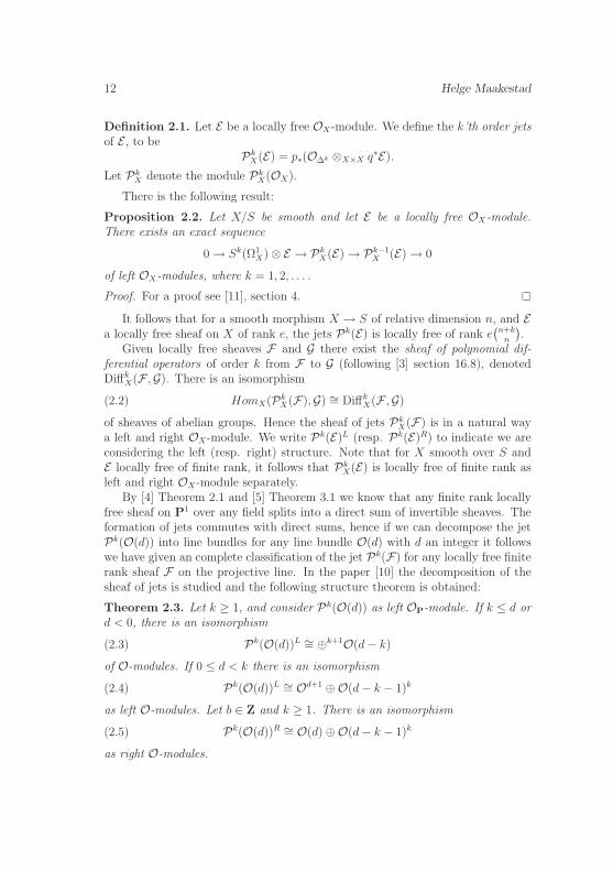
12 Helge Maakestad
Definition 2.1. Let E be a locally free OX-module. We define the k’th order jetsof E , to be
PkX(E) = p∗(O∆k ⊗X×X q∗E).
Let PkX denote the module Pk
X(OX).
There is the following result:
Proposition 2.2. Let X/S be smooth and let E be a locally free OX-module.There exists an exact sequence
0 → Sk(Ω1X)⊗ E → Pk
X(E) → Pk−1X (E) → 0
of left OX-modules, where k = 1, 2, . . . .
Proof. For a proof see [11], section 4.
It follows that for a smooth morphism X → S of relative dimension n, and Ea locally free sheaf on X of rank e, the jets Pk(E) is locally free of rank e
(n+k
n
).
Given locally free sheaves F and G there exist the sheaf of polynomial dif-ferential operators of order k from F to G (following [3] section 16.8), denotedDiffk
X(F ,G). There is an isomorphism
(2.2) HomX(PkX(F),G) ∼= Diffk
X(F ,G)
of sheaves of abelian groups. Hence the sheaf of jets PkX(F) is in a natural way
a left and right OX-module. We write Pk(E)L (resp. Pk(E)R) to indicate we areconsidering the left (resp. right) structure. Note that for X smooth over S andE locally free of finite rank, it follows that Pk
X(E) is locally free of finite rank asleft and right OX-module separately.
By [4] Theorem 2.1 and [5] Theorem 3.1 we know that any finite rank locallyfree sheaf on P1 over any field splits into a direct sum of invertible sheaves. Theformation of jets commutes with direct sums, hence if we can decompose the jetPk(O(d)) into line bundles for any line bundle O(d) with d an integer it followswe have given an complete classification of the jet Pk(F) for any locally free finiterank sheaf F on the projective line. In the paper [10] the decomposition of thesheaf of jets is studied and the following structure theorem is obtained:
Theorem 2.3. Let k ≥ 1, and consider Pk(O(d)) as left OP-module. If k ≤ d ord < 0, there is an isomorphism
(2.3) Pk(O(d))L ∼= ⊕k+1O(d− k)
of O-modules. If 0 ≤ d < k there is an isomorphism
(2.4) Pk(O(d))L ∼= Od+1 ⊕O(d− k − 1)k
as left O-modules. Let b ∈ Z and k ≥ 1. There is an isomorphism
(2.5) Pk(O(d))R ∼= O(d)⊕O(d− k − 1)k
as right O-modules.
Jet bundles on projective space 13
Proof. See [10].
The proof of this result is done by calculating and diagonalizing the transitionmatrix of the jet bundle. The result gives a complete classification of the jets ofan arbitrary locally free sheaf on the projective line as left and right module overthe structure sheaf.
3 On the left and right P -module structure on
the projective line
In this section we give a complete classification of the left and right P -modulestructure of the jets on the projective line over a field of characteristic zero usingthe same techniques as in [8].
Let in general V be a finite dimensional vector space over a field F of char-acteristic zero. Any affine algebraic group G is a closed subgroup of GL(V ) forsome V , and given any closed subgroup H ⊆ G, there exists a quotient mapG → G/H with nice properties. The variety G/H is smooth and quasi projec-tive, and the quotient map is universal with respect to H-invariant morphismsof varieties. F -rational points of the quotient G/H correspond to orbits of Hin G (see [7], section I.5). Moreover: any finite-dimensional H-module ρ givesrise to a finite rank G-homogeneous vector bundle E = E(ρ) and by [1], chapter4 this correspondence sets up an equivalence of categories between the categoryof linear finite dimensional representations of H and the category of finite rankG-homogeneous vector bundles on G/H. There exists an equivalence of categoriesbetween the category of finite rank G-homogeneous vector bundles and the cat-egory of finite rank locally free sheaves with a G-linearization, hence we will usethese two notions interchangeably.
Fix a line L in V , and let P be the closed subgroup of SL(V ) stabilizing L.The quotient SL(V )/P is naturally isomorphic to projective space P parametrizinglines in V , and if we choose a basis e0, · · · , en for V , the quotient map
π : SL(V ) → P
can be chosen to be defined as follows: map any matrix A to its first column-vector.It follows that π is locally trivial in the Zariski topology, in fact it trivializes overthe basic open subsets Ui of projective space. One also checks that any SL(V )-homogeneous vectorbundle on P trivializes over the basic open subsets Ui. Anyline bundle O(d) on projective space is SL(V )-homogeneous coming from a uniquecharacter of P since SL(V ) has no characters. The sheaf of jets Pk(O(d)) is asheaf of bi-modules, locally free as left and right O-module separately. It has aleft and right SL(V )-linearization, hence we may classify the P -module structureof Pk(O(d)) corresponding to the left and right structure, and that is the aim ofthis section.
14 Helge Maakestad
The calculation of the representations corresponding to Pk(O(d)) as left andright P -module is contained in Theorems 3.4 and 3.6. As a byproduct we obtainthe classification of the splitting type of the jet bundles obtained in [10]: this isCorollaries 3.5 and 3.7.
Let, in the following section V be a vector space over F of dimension two.P = SL(V )/P is the projective line parametrizing lines in V . There exists twoexact sequences of P -modules.
0 → L → V → Q → 0
and0 → m → V ∗ → L∗ → 0,
and one easily sees that m ∼= L as P -module.Let p, q : P×P → P be the canonical projection maps, and let I ⊆ OP×P be
the ideal of the diagonal. Let O∆k = OP×P/Ik+1 be the k′th order infinitesimalneighborhood of the diagonal. Recall the definition of the sheaf of jets:
Definition 3.1. Let E be an OP-module. Let k ≥ 1 and let
Pk(E) = p∗(O∆k ⊗ q∗E)
be the k’th order sheaf of jets of E .
If E is a sheaf with an SL(V )-linearization, it follows that Pk(E) has a canonicalSL(V )-linearization. There is an exact sequence:
(3.1) 0 → Ik+1 → OP×P → O∆k → 0.
Apply the functor R p∗(− ⊗ q∗O(d)) to the sequence 3.1 to obtain a long exactsequence of SL(V )-linearized sheaves
(3.2) 0 → p∗(Ik+1 ⊗ q∗O(d)) → p∗q∗O(d) → Pk(O(d))L →
R1 p∗(Ik+1 ⊗ q∗O(d)) → R1 p∗q∗O(d) → R1 p∗(O∆k ⊗ q∗O(d)) → · · ·of OP-modules. We write Pk(O(d))L to indicate that we use the left structureof the jets. We write Pk(O(d))R to indicate right structure. The terms in thesequence 3.2 are locally free since they are coherent and any coherent sheaf withan SL(V )-linearization is locally free.
Proposition 3.2. Let E be an SL(V )-linearized sheaf with support in ∆ ⊆ P×P.For all i ≥ 1 the following holds:
Ri p∗(E) = Ri q∗(E) = 0.
Jet bundles on projective space 15
Proof. Let x ∈ P be the distinguished point and consider the fiber diagram
Pj //
p,q²²
P×P
p,q
²²Spec(κ(x)) i // P
Since Ri p∗(E) and Ri q∗(E) have an SL(V )-linearization it is enough to check thestatement of the lemma on the fiber at x. We get by [6], Proposition III.9.3isomorphisms
Ri p∗(E)(x) ∼= Ri p∗(j∗E)
andRi q∗(E)(x) ∼= Ri q∗(j∗E),
and since j∗E is supported on a zero-dimensional scheme, the lemma follows.
It follows from the Lemma that R1 p∗(O∆k⊗q∗O(d)) = R1 q∗(O∆k⊗q∗O(d)) =0 sinceO∆k⊗q∗O(d) is supported on the diagonal. Hence we get an exact sequenceof P -modules when we pass to the fiber of 3.2 at the distinguished point x ∈ P.Let m ⊆ OP be the sheaf of ideals of x. By [6] Theorem III.12.9 and Lemma 3.2we get the following exact sequence of P -modules:
(3.3) 0 → H0(P,mk+1 ⊗O(d)) → H0(P,O(d)) → Pk(O(d))(x) →
H1(P, mk+1 ⊗O(d)) → H1(P,O(d)) → 0.
Proposition 3.3. Let k ≥ 1 and d < k. Then there is an isomorphism
H1(P, mk+1 ⊗O(d)) ∼= Symk+1(L)⊗ Symk−d−1(V )
of P -modules.
Proof. There is an isomorphism of sheaves O(−k − 1) ∼= mk+1 defined as follows:
x−k−10 → tk+1
on the open set D(x0) where t = x1/x0. On the open set D(x1) it is defined asfollows:
x−k−11 → 1.
We get an isomorphism O(d − k − 1) ∼= mk+1 ⊗ O(d) of sheaves, but the corre-sponding inclusion of sheaves
O(d− k − 1) → O(d)
16 Helge Maakestad
is not a map of P -linearized sheaves, since it is zero on the fiber at x. Hence wemust twist by the character of mk+1 = O(−k− 1) when we use Serre-duality. Weget
H1(P,mk+1 ⊗O(d)) ∼= Symk+1(L)⊗ H0(P,O(k − d− 1))∗ ∼=Symk+1(L)⊗ Symk−d−1(V ),
and the proposition follows.
We first give a complete classification of the left P -module structure of thejets. The result is the following.
Theorem 3.4. Let k ≥ 1, and consider Pk(O(d)) as left OP-module. If k ≤ d,there exists an isomorphism
(3.4) Pk(O(d))L(x) ∼= Symk−d(L∗)⊗ Symk(V ∗)
of P -modules. If d ≥ 0 there exist an isomorphism
(3.5) Pk(O(−d))L(x) ∼= Symk+d(L)⊗ Symk(V )
of P -modules. If 0 ≤ d < k there exist an isomorphism
(3.6) Pk(O(d))L(x) ∼= Symd(V ∗)⊕ Symk+1(L)⊗ Symk−d−1(V )
of P -modules.
Proof. The isomorphism from 3.4 follows from Theorem 2.4 in [8]. We prove theisomorphism 3.5: Since −d < 0 we get an exact sequence
0 → Pk(O(−d))(x) → H1(P,mk+1 ⊗O(−d)) → H1(P,O(−d)) → 0
of P -modules. By proposition 3.3 we get the exact sequence of P -modules
0 → Pk(O(−d))L(x) → Symk+1(L)⊗ Symd+k−1(V ) → Symd−2(V ) → 0.
The map on the right is described as follows: dualize to get the following:
Symd−2(V ∗) ∼= Symk+1(L∗)⊗ Symk+1(L)⊗ Symd−2(V ∗) ∼=Symk+1(L∗)⊗ Symk+1(m)⊗ Symd−2(V ∗) → Symk+1(L∗)⊗ Symd+k−1(V ∗).
The map is described explicitly as follows:
f(x0, x1) → xk+10 ⊗ xk+1
1 f(x0, x1).
If we dualize this map we get a map
Symk+1(L)⊗ Symd+k−1(V ) → Symd−2(V ),
Jet bundles on projective space 17
given explicitly as follows:
ek+10 ⊗ f(e0, e1) → φ(f(e0, e1)),
where φ is k + 1 times partial derivative with respect to the e1-variable. Thereexists a natural map
Symk+d(L)⊗ Symk(V ) → Symk+1(L)⊗ Symd+k−1(V )
given byek+d0 ⊗ f(e0, e1) → ek+1
0 ⊗ ed−10 f(e0, e1)
and one checks that this gives an exact sequence
0 → Symk+d(L)⊗ Symk(V ) → Symk+1(L)⊗ Symd+k−1(V ) →Symd−2(V ) → 0,
hence we get an isomorphism
Pk(O(−d))L(x) ∼= Symk+d(L)⊗ Symk(V ),
and the isomorphism from 3.5 is proved. We next prove isomorphism 3.6: Byvanishing of cohomology on the projective line we get the following exact sequence:
0 → H0(P,O(d)) → Pk(O(d))L(x) → H1(P, mk+1 ⊗O(d)) → 0.
We get by Proposition 3.3 an exact sequence of P -modules
0 → Symd(V ∗) → Pk(O(d))L(x) → Symk+1(L)⊗ Symk−d−1(V ) → 0.
It splits because of the following:
Ext1P (Symk+1(L)⊗ Symk−d−1(V ), Symd(V ∗)) =
Ext1P (ρ, Symk+1(L∗)⊗ Symk−d−1(V ∗)⊗ Symk−1(V ∗)).
Here ρ is the trivial character of P . Since there is an equivalence of categoriesbetween the category of P -modules and SL(V )-linearized sheaves we get again byequivariant Serre-duality
Ext1P (ρ, Symk+1(L∗)⊗ Symk−d−1(V ∗)⊗ Symk−1(V ∗)) = H1(P,O(k + 1)⊗ E1) =
⊕r1 H1(P,O(k + 1)) = ⊕r1 H0(P,O(−k − 3))∗ = 0.
Here E1 is the SL(V )-linearized sheaf corresponding to Symk−d−1(V ∗)⊗Symk−1(V ∗)and r1 is the rank of E1. Hence we get
Pk(O(d))L(x) ∼= Symd(V ∗)⊕ Symk+1(L)⊗ Symk−d−1(V ),
and the isomorphism from 3.6 is proved hence the theorem follows.
18 Helge Maakestad
As a corollary we get a result on the splitting type of the jets as left moduleon the projective line.
Corollary 3.5. The splitting type of Pk(O(d)) as left OP-module is as follows:If k ≥ 1 and d < 0 or d ≥ k there exist an isomorphism
(3.7) Pk(O(d))L ∼= ⊕k+1O(d− k)
of left O-modules. If 0 ≤ d < k there exist an isomorphism
(3.8) Pk(O(d))L ∼= Od+1 ⊕O(−k − 1)k−d
of left O-modules.
Proof. This follows directly from Theorem 3.4.
We next give a complete classification of the right P -module structure of thejets. The result is the following.
Theorem 3.6. Let k ≥ 1 and consider Pk(O(d)) as right module. If d > 0 thereexist an isomorphism
(3.9) Pk(O(−d))R(x) ∼= Symd(L)⊕ Symk+d+1(L)⊗ Symk−1(V )
of P -modules. If d ≥ 0 there exist an isomorphism
(3.10) Pk(O(d))R(x) ∼= Symd(L∗)⊕ Symd−k−1(L∗)⊗ Symk−1(V )
as P -modules.
Proof. We prove the isomorphism 3.9: Using the functor Ri q∗(−⊗ q∗O(−d)) weget a long exact sequence of SL(V )-linearized sheaves
0 → q∗(Ik+1)⊗O(−d) → q∗q∗O(−d) → Pk(O(−d))R → R1 q∗(Ik+1)⊗O(−d) →
R1 q∗(OP×P)⊗O(−d) → 0.
It is exact on the right because of Proposition 3.2. Here we write Pk(O(d))R toindicate we use the right structure of the jets. We take the fiber at x ∈ P andusing Cech-calculations for coherent sheaves on the projective line, we obtain thefollowing exact sequence of P -modules:
0 → H0(P,OP)⊗O(−d)(x) → Pk(O(−d))R(x) → H1(P,mk+1)⊗O(−d)(x) → 0
Hence we get by Proposition 3.3 the following exact sequence of P -modules:
0 → Symd(L) → Pk(O(−d))R(x) → Symd(L)⊗ Symk+1(L)⊗ Symk−1(V ) → 0
Jet bundles on projective space 19
It is split exact because of the following argument using Ext’s and equivariantSerre-duality:
Ext1P (Symd+k+1(L)⊗ Symk−1(V ), Symd(L)) = Ext1
P (ρ, Symk+1(L∗)⊗ Symk(V ∗)),
where ρ is the trivial character of P . By equivariant Serre duality we get
Ext1P (ρ, Symk+1(L∗)⊗ Symk(V ∗)) = H1(P,O(k + 1)⊗ E2) =
= ⊕r2 H0(P,O(−k − 3))∗ = 0.
Here E2 is the abstract vector bundle corresponding to Symk(V ∗) and r2 is therank of E2. Hence we get the desired isomorphism
Pk(O(−d))R(x) ∼= Symd(L)⊕ Symd+k+1(L)⊗ Symk−1(V ),
and isomorphism 3.9 is proved.We next prove the isomorphism 3.10: Using the functor Ri q∗(−⊗ q∗O(d)) we
get a long exact sequence of SL(V )-linearized sheaves
0 → q∗(Ik+1)⊗O(d) → q∗q∗O(d) → Pk(O(d))R → R1 q∗(Ik+1)⊗O(d) →R1 q∗(OP×P)⊗O(d) → 0.
We take the fiber at x ∈ P and using Cech-calculations for coherent sheaves onthe projective line, we obtain the following exact sequence of P -modules:
0 → H0(P,OP)⊗O(d)(x) → Pk(O(d))R(x) → H1(P,mk+1)⊗O(d)(x) → 0.
Proposition 3.3 gives the following sequence of P -modules
0 → Symd(L∗) → Pk(O(d))R(e) → Symd(L∗)⊗ Symk+1(L)⊗ Symk−1(V ) → 0
It splits because of the following Ext and equivariant Serre-duality argument:
Ext1P (Symd(L∗)⊗ Symk+1(L)⊗ Symk−1(V ), Symd(L∗)) =
Ext1P (ρ, Symk+1(L∗)⊗ Symk−1(V ∗)).
Let E3 be the vector bundle corresponding to Symk−1(V ∗) and let r3 be its rank.We get
Ext1P (ρ, Symk+1(L∗)⊗ Symk−1(V ∗)) = H1(P,O(k + 1)⊗ E3) =
= ⊕r3 H0(P,O(−k − 3))∗ = 0,
hence we get the isomorphism
Pk(O(d))R(x) ∼= Symd(L∗)⊕ Symd−k−1(L∗)⊗ Symk−1(V ),
and isomorphism 3.10 follows.
20 Helge Maakestad
As a corollary we get a result on the splitting type of the jets as right module.
Corollary 3.7. Let k ≥ 1 and d ∈ Z. There exist an isomorphism
(3.11) Pk(O(d))R ∼= O(d)⊕O(d− k − 1)k
of right OP-modules.
Proof. This follows directly from Theorem 3.6.
Note that Corollary 3.5 and 3.7 recover Theorem 3.4, hence we have usedelementary properties of representations of SL(V ) to classify sheaves of left andright modules on the projective line over any field of characteristic zero.
On projective space of higher dimension there is the following result: LetPN = SL(V )/P where P is the subgroup fixing a line, and let O(d) be the linebundle with d ∈ Z. It follows O(d) has a canonical SL(V )-linearization.
Theorem 3.8. For all 1 ≤ k < d, the representation corresponding to Pk(O(d))L
is Symd−k(L∗)⊗ Symk(V ∗).
Proof. See [8].
Note that the result in Theorem 3.8 is true over any field F if char(F ) > n.
Corollary 3.9. For all 1 ≤ k < d, Pk(O(d)) decompose as left O-module as
⊕(N+kN )O(d− k).
Proof. See [8].
Note. Theorem 3.4 and 3.6 give a complete classification of the structure ofthe jets as left and right P -module for any line bundle O(d).
Acknowledgements. Thanks to Michel Brion and Dan Laksov for comments.
References
[1] D. N. Akhiezer, Lie group actions in complex analysis, Aspects of Mathemat-ics, Vieweg (1995)
[2] A. Borel, Linear algebraic groups, Graduate Texts in Mathematics no. 126,Springer Verlag (1991)
[3] A. Grothendieck, Elements de geometrie algebrique IV4,Etude locale desschemas et des morphismes de schemas , Publ. Math. IHES 32 (1967)
[4] A. Grothendieck, Sur la classification des fibres holomorphes sur la sphere deRiemann, Amer. J. Math. 79 (1957)
Jet bundles on projective space 21
[5] G. Harder, Gruppenschemata uber vollstandigen Kurven, Invent. Math. 6(1968)
[6] R. Hartshorne, Algebraic geometry, Graduate Texts in Mathematics no. 52,Springer Verlag (1977)
[7] J. C. Jantzen, Representations of algebraic groups, Pure and Applied Math-ematics (131), Academic Press (1987)
[8] H. Maakestad, A note on the principal parts on projective space and linearrepresentations, Proc. Amer. Math. Soc. 133 (2005) no. 2
[9] H. Maakestad, Modules of principal parts on the projective line, Ark. Mat.42 (2004) no. 2
[10] H. Maakestad, Principal parts on the projective line over arbitrary rings,Manuscripta Math. 126 (2008), no. 4
[11] D. Perkinson, Curves in grassmannians, Trans. Amer. Math. Soc 347 (1995)no. 9
[12] D. Perkinson, Principal parts of line bundles on toric varieties, CompositioMath. 104, 27-39, (1996)
[13] R. Piene, G. Sacchiero, Duality for rational normal scrolls, Comm. in Alg. 12(9), 1041-1066, (1984)
[14] S. di Rocco, A. J. Sommese, Line bundles for which a projectivized jet bundleis a product, Proc. Amer. Math. Soc. 129, (2001), no.6, 1659–1663
[15] A. J. Sommese, Compact complex manifolds possessing a line bundle with atrivial jet bundle, Abh. Math. Sem. Univ. Hamburg 47 (1978)
Helge MaakestadInstitut [email protected]

Travaux mathematiques, Volume 18 (2008), 23–25, c© Universite du Luxembourg
Around Birkhoff Theorem1
by O.Petrenko and I.V.Protasov
Abstract
Let X be a topological space, f : X → X be a mapping (not necessarilycontinuous). A point x ∈ X is recurrent if x is a limit point of the orbit(fn(x))n∈N. We prove that, for a Hausdorff space X, every bijection has arecurrent point if and only if X is either finite or a one-point compactifica-tion of an infinite discrete space.
1 Introduction
Let X be a topological space, f : X → X be an arbitrary mapping. A pointx ∈ X is said to be recurrent if for every neighbourhood U of x and every n ∈ ω,there exists m > n such that fm(x) ∈ U (in other words, x is a limit point ofthe orbit (fn(x))n∈N). By Birkhoff Theorem ([1],[2]), every continuous mappingf : X → X of a compact space X has a recurrent point. We are going to provethe following ”discontinuous” version of Birkhoff Theorem.
Theorem 1.1. For a Hausdorff space X, the following statements are equivalent:(i) every mapping f : X → X has a recurrent point;(ii) every bijection f : X → X has a recurrent point;(iii) X is either finite or a one-point compactification of an infinite discrete
space.
2 Auxiliary lemmas
For proof of Theorem, we need two lemmas. Remind that a subspace Y of a topo-logical space X is discrete in itself if, for every y ∈ Y there exists a neighbourhoodU of y, such that U ∩ Y = y.Lemma 2.1. For every infinite Hausdorff space X, there exists a disjoint family ofcountable discrete in itself subspaces Xα : α ∈ A such that either X\ ⋃
α∈AXα = ∅
or X \ ⋃α∈A
Xα is a singleton x and x is a limit point of every subspace Xα.
1Received: October 7, 2007
24 O.Petrenko and I.V.Protasov
Proof. We use the following auxiliary statement: every infinite Hausdorff space Shas a countable subspace D discrete in itself. Indeed, if S is discrete, it is clear.Otherwise, we fix some non-isolated point s ∈ S, choose an arbitrary elementd0 ∈ S, d0 6= s and the disjoint open neighbourhoods U0, V0 of d0 and s. Thenwe pick an arbitrary element d1 ∈ V0 and disjoint open neighbourhoods U1, V1
of d1 and s such that U1 ⊆ V0, V1 ⊆ V0. After N steps we get the sequence(dn)n∈N of elements of S and the sequence (Un)n∈N of its neighbourhoods suchthat Ui ∩ Uj = ∅ for all distinct i, j ∈ N. Then D = dn : n ∈ N is discrete initself.
By Zorn Lemma, there exists a maximal disjoint family Xα : α ∈ A ofcountable discrete in itself subspaces of X. By the auxiliary statement, applyingto S = X \ ⋃
α∈AXα, we conclude that X \ ⋃
α∈AXα is finite.
We assume that X \ ⋃α∈A
Xα 6= ∅ and take an arbitrary element y ∈ X \ ⋃α∈A
Xα.
If y is not a limit point of some subspace Xβ, we put X ′β = Xβ∪y and X ′
α = Xα
for all α 6= β. Then X ′α : α ∈ A is a disjoint family of countable discrete in itself
subspaces of X and |X \ ⋃α∈A
Xα| > |X \ ⋃α∈A
X ′α|. Repeating this arguments, we
may suppose that every element y ∈ X \ ⋃α∈A
Xα is a limit point of each subspace
Xα.If |X \ ⋃
α∈AXα| > 1, we fix two arbitrary points y, z ∈ X \ ⋃
α∈AXα and its
disjoint neighbourhoods U and V . For one fixed α0 ∈ A we put
X ′α0
= (Xα0 ∩ U) ∪ z, X ′′α0
= (Xα0 \ U) ∪ y
For every α ∈ A \ α0, we put
X ′α = (Xα ∩ U), X ′′
α = (Xα \ U)
Then X ′α, X ′′
α : α ∈ A is a disjoint family of countable subspaces discrete initself, and |X \ ⋃
α∈A(X ′
α ∪ X ′′α)| < |X \ ⋃
α∈AXα|. Repeating the arguments of
above and this paragraphs, after finite number of steps we get a desired family ofsubspaces of X.
Lemma 2.2. An infinite Hausdorff space X is a one-point compactification of adiscrete space if and only if, for every partition X =
⊔α∈A
Xα of X to countable
subspaces, at least one subspace of the partition is not discrete in itself.
Proof. Let X be a one-point compactification of discrete subspace D, x = X\D.Given any partition X =
⊔α∈A
Xα of X to countable subspaces, we take β ∈ Asuch that x ∈ Xβ. Then x is non-isolated point of Xβ, so Xβ is not discrete initself.
Around Birkhoff Theorem 25
On the other hand, let X satisfy the partition condition of lemma. We take thefamily Xα : α ∈ A given by Lemma 1. If X\ ⋃
α∈AXα = ∅, we get a contradiction
to the partition condition, so X \ ⋃α∈A
Xα = x. We assume that X \V is infinite
for some neighbourhood V of x, and choose a countable discrete in itself subspaceD of X \V , put Y = D∪x and Yα = Xα\D. Since x is a limit point of each Xα,every subspace Yα is countable. Then X = Y ∪ ⋃
α∈AYα, each subspace Y, Yα, α ∈ A
is countable and discrete in itself, so we again arrive on the contradiction with thepartition condition. Hence, X \ V is finite for every neighbourhood V of x, so Xis a one-point compactification of discrete space X \ x.
3 Proof of main result
Proof of Theorem 1. The implication (i)⇒(ii) is trivial.To show (ii)⇒(iii), we assume that X is infinite, but X is not a one-point
compactification of a discrete space. By Lemma 2, there is a partition X =⊔
α∈AXα
such that each cell Xα is countable and discrete in itself. For every α ∈ A, we fixsome bijection fα : Xα → Xα without periodic points. Put f =
⊔α∈A fα. Then
f : X → X is a bijection without recurrent points.If X is finite then every mapping f : X → X has a periodic point which is
recurrent. Let X be a one-point compactification of an infinite discrete space D,x = X \D, f : X → X. If x is not a limit point of the orbit fn(x) : n ∈ N,then there exists a neighbourhood U of x and n ∈ N such that fm(x) /∈ U forevery m > n. Since X \ U is finite, at least one point from X \ U is periodic.Hence, (iii)⇒(i).
¤Problem 3.1. Detect all Hausdorff spaces such that every continuous mappingf : X → X has a recurrent point. Does there exist non-countably compact spacewith this property?
References
[1] G.D. Birkhoff, Dynamical systems, Amer. Math. Soc. Coll. Publ., 9, 1927.
[2] R.Ellis, Lectures on topological dynamics, Benjamin, New York, 1969.
Department of Cybernetics,Kyiv National University,Volodimirska 64, Kyiv 01033,Ukrainee-mail: [email protected]

Travaux mathematiques, Volume 18 (2008), 27–37, c© Universite du Luxembourg
Zero-emission surfaces of a moving electron1
by Yu. A. Aminov
Abstract
The motion of an electron in a constant magnetic field and its electro-magnetic emission are presented. We consider a zero-emission ruled surfaceof the electron. The theorem on existence and uniqueness of a secondelectron with the same zero-emission surface is proved. The notion of ”con-jugate” electron is introduced and the formula for distance between two”conjugate” electrons is given.
Mathematics Subject Classification. Primary 53A05, 78A35, 78A40;Secondary 53A25.
Keywords. Ruled surface, helix, electron, electromagnetic field.
“...Maxwell has developed a complete mathematicaltheory to describe electromagnetism and showed that
charges moving with acceleration emit...”Abdus Salam “Unification of forces”
1 Introduction
The classical problem about a motion of a charge in a constant magnetic field iswell investigated. It seems that impossible to discover something new here. Butgeometrical point of view allows to add interesting knowledge to this old problem.It is well known, that the motion of a charge with acceleration be accompaniedby emission of electromagnetic field. This emission is going from every point ofthe trajectory of the charge at moment, when the charge passes this point. If thecharge is an electron, so this emission is considerable. For example, the motionof the stream of electrons in a synchrotron gives the strong synchrotron emission.For proton, which mass is at 2000 times larger than electron one, his emission isnot such important. Therefore we speak further about the electron motion.
1Received: October 23, 2007
28 Yuriy Aminov
There exists physical theory to describe this emission, which we use in presentarticle. The formula for emission, represented in [3], gives two directions, startingfrom the point of trajectory, for which the emission is equal to zero. We considerthe ruled surface in E3 with the trajectory as a directrix and a generatrix, goingin the direction with emission equal to zero. More precisely, we must take theray in this direction, but complete surface is more comfortable for consideration.That’s the way ” zero- emission surface” arises.
As there exist two directions with emission equal to zero, so there are twozero-emission surfaces.
This surface has some interesting geometrical properties. In the section 1 weshow that the trajectory is an asymptotic curve on it. It is natural to put thefollowing question: does determined zero-emission surface the electron, which itsgenerate. It is purely mathematical question about uniqueness. If to speak moreprecisely so the talk is going about the trajectory and the law of motion alongthis trajectory. We show that here the uniqueness does not have place. In thesection 2 the following theorem is been proving
Theorem 1.1. For an electron in a constant magnetic field every zero-emissionsurface contains a unique second electron such that these electrons lie throughouttheir motion in the common zero-emission line.
Denote the first electron Q1 and the second Q2. We indicate the place for Q2
and calculate the distance between Q1 and Q2, which is a constant.In the section 2 the notion of geometrically consistent (coherent) motion of the
third electron Q3 with respect to the electrons Q1, Q2 is given. It is motion, whenQ3 lies on the straight -line Q1Q2 and distance q between Q1 and Q3 is constant.We use the word ”geometrically” for emphasize that here we ignore influence byCoulomb fields and emissions of every electrons each other. It have place
Theorem 1.2. There exists a motion of electron Q3 along helix q = const on thezero-emission surface geometrically consistent (coherent) with the motions of Q1
and Q2.
2 The trajectory of an electron as the asymp-
totic line on the zero-emission surface
Let us consider the motion of a point charge ( for example, an electron) in aconstant magnetic field H = H0 = const within the bounds of classical electro-dynamics. If the motion is with acceleration then there exists an emission of
Zero-emission surfaces of a moving electron 29
electromagnetic field. In the classical electrodynamics the emission is describedby two vector fields - electric Eemit and magnetic Bemit. The fields Eemit and Bemit
at different points have different intensities and vectors. We have found some cor-relation between emission and some ruled surfaces (see [1], [2]) and present it herewith some new details.
If x(t) is a vector position of a point of the electron trajectory, then the equa-tion of motion is the following
d2x
dt2= − e
mc[dx
dtH0], (1)
where t is the time, e is the electric charge, m is its mass and c is the light velocity.It is well known that the charge moves along a straight line or a circle or a helix.Denote
µ0 = − e
mc.
By integration of (1) we obtain
dx
dt= µ0[xH0] + q, (2)
where q = qi is the constant vector. Let e1, e2, e3 be an orthogonal frame in E3
and H0 = he3. We can rewrite Equation (2) in the form of a system of equations
dx1
dt= µ0hx2 + q1,
dx2
dt= −µ0hx1 + q2, (3)
dx3
dt= q3.
Let the initial data for t = 0 be
x1(0) = x10, x2(0) = x20, x3(0) = 0,dxi(0)
dt= ai, i = 1, 2, 3.
Introduce new coordinates
x1 = x1 − q2
µ0h, x2 = x2 +
q1
µ0h, x3 = x3.
Then the Equations (3) will be as follows
dx1
dt= µ0hx2,
dx2
dt= −µ0hx1,
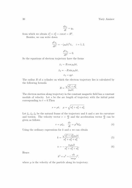
30 Yuriy Aminov
dx3
dt= q3,
from which we obtain x21 + x2
2 = const = R2.Besides, we can write down
d2xi
dt2= −(µ0h)2xi, i = 1, 2,
d2x3
dt2= 0.
So the equations of electron trajectory have the forms
x1 = R cos µ0ht,
x2 = −R sin µ0ht,
x3 = q3t.
The radius R of a cylinder on which the electron trajectory lies is calculated bythe following formula
R =
√a2
1 + a22
|µ0h| .
The electron motion along trajectory in the constant magnetic field has a constantmodule of velocity. Let s be the arc length of trajectory with the initial pointcorresponding to t = 0.Then
s = µt, µ =√
a21 + a2
2 + a23.
Let ξ1, ξ2, ξ3 be the natural frame of the trajectory and k and κ are its curvatureand torsion. The velocity vector v = dx
dtand the acceleration vector dv
dtcan be
given as follows
v = µξ1,dv
dt= µ2kξ2. (4)
Using the ordinary expressions for k and κ we can obtain
k =
√a2
1 + a22|µ0h|
a21 + a2
2 + a23
. (5)
κ = − a3µ0h
a21 + a2
2 + a23
. (6)
Hence
k2 + κ2 = (eh
mcµ)2,
where µ is the velocity of the particle along its trajectory.
Zero-emission surfaces of a moving electron 31
Now we consider the emission of an electron moving along a helix. Since theelectron has a curvilinear trajectory, so its acceleration is non-zero and therefore itradiates an electromagnetic field. Assume that the origin of coordinates coincideswith the current position of the electron. We denote this point by Q1.We supposethat electron lies at this point at time t.
Let r be the vector position of a point in space. Then the electric and magneticemission at a point with the vector position r can be given by the followingexpressions (see [3](19.17), [4](14.35))
Eemit(r, t′) =
e
4πε0c2l3[r, [r − v|r|
c,dv
dt]], (7)
Bemit(r, t′) =
[r, Eemit]
|r|c ,
where the right sides are taken for t, t′ = t + |r|c, l = |r| − (vr)/c and ε0 is some
physical constant.Two natural ruled surfaces appear which are constructed using the directions
with zero emission.According to Equation (7) for the direction r with zero-emission the vector
product [r − v|r|c
, ξ2] is proportional to r. Let ν be the unit vector along r.Takinginto consideration the formula (4), we obtain
[ν − µ
cξ1, ξ2] = λν, (9)
where λ is an unknown coefficient. Let us suppose that λ 6= 0. Then we concludethat ν lies in the plane of ξ1, ξ3. We have
ν = ν1ξ1 + ν3ξ3, (ν1)2 + (ν3)2 = 1.
Equation (9) can be rewritten as follows
ν1ξ3 − ν3ξ1 − µ
cξ3 = λ(ν1ξ1 + ν3ξ3).
Therefore we have two equations
−ν3 = λν1,
ν1 − µ
c= λν3,
from which we obtain(ν1)2 + (ν3)2 − µ
cν1 = 0,
and 1 = µcν1. But the velocity of an electron is less than c. The latter equality
is impossible. Hence λ = 0. The equation for zero-emission direction is of thefollowing form
[ν − µ
cξ1, ξ2] = 0. (10)
32 Yuriy Aminov
This equation is given in [ 3], [4] . From (10) we can conclude that the zero-emission direction lies in the osculation plane of trajectory
ν =µ
cξ1 + λξ2,
where λ is the coefficient. As ν is the unit vector, λ can be given by two expressions
λ = ±√
1− (µ
c)2.
So, there are two zero-emission directions ν1 and ν2, which lie symmetrically withrespect to ξ1. Let φ > 0 be the angle between ν1 and ξ1. Evidently cos φ = µ
c. We
call φ the angle of zero emission. We have
ν1 = cos φξ1 + sin φξ2,
ν2 = cos φξ1 − sin φξ2
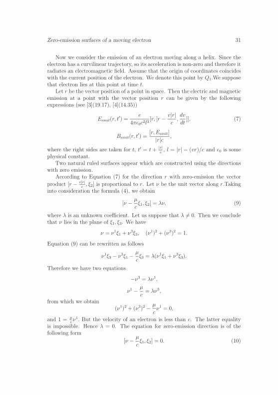
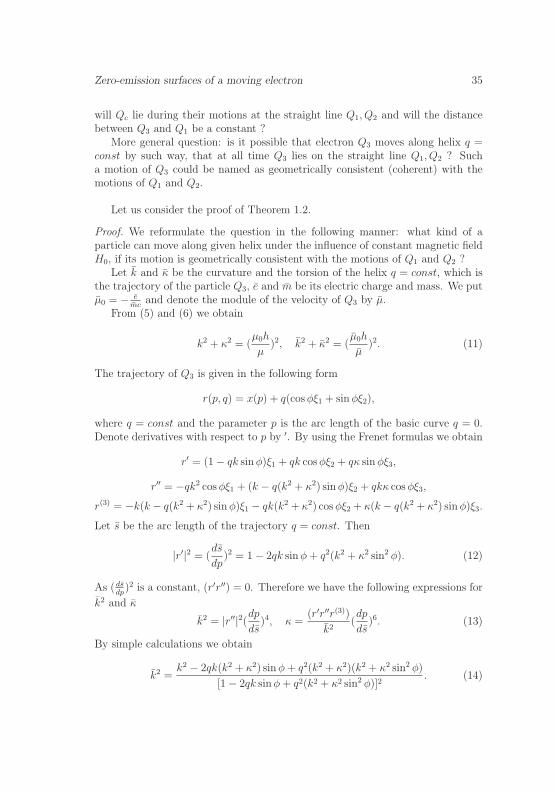
Drawing through every point of the helix a straight line in the direction ν1 weobtain a ruled surface Ψ1(Q1), see Fig.1. It is natural to call it a zero-emissionsurface.
Therefore, zero-emission surface of a moving electron is the regular ruledsurface with the trajectory of the electron as a directrix and a generatrix, goingin the direction with the electron emission from the point of trajectory equal tozero.
By analogy, we obtain a ruled surface Ψ2(Q1).Since the principal normal to the trajectory lies in the tangent plane to surface
Ψi(Q1), this curve is an asymptotic line.
Remark. One can also construct a ruled zero-emission surface for the generalcase of a radiating electron ( not necessarily in a constant magnetic field). Thenthe trajectory of the particle will be an asymptotic line on this surface.
Consider now the following question:
Does there exist another electron Q2 in the zero-emission straightline of Q1 such that its zero-emission straight line at every moment tcoincides with that of the first electron Q1?
Zero-emission surfaces of a moving electron 33
Fig. 1
Now we can prove Theorem 1.1.
Proof. By the existence of a second electron we mean the existence of a trajectoryand the existence of a motion of the electron along this trajectory.
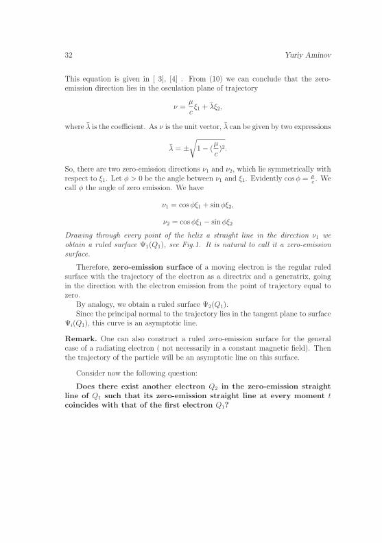
We shall say that electrons Q1 and Q2 are ”conjugate” on the surface Ψ1(Q1).
Fig. 2
The place of electron Q2 can be indicated in a simple way. The point Q2 is theintersection point of the ray from Q1 in the direction ν1 with the cylinder carryingthe trajectory of Q1. It is obvious that this intersection point describes a helixparallel to the helix of the point Q1. The uniqueness of this second electron is aconsequence of the following lemmas. Let us write down the equation of surfaceΨ1(Q1)
r(p, q) = x(p) + q(cos φξ1 + sin φξ2),
34 Yuriy Aminov
where x(p) is the vector position of the trajectory of Q1 and the parameter p isits arc length. Denote
T = 2k sin φ− q(k2 + κ2 sin2 φ).
Lemma 2.1. Asymptotic lines distinct from straight line generators have the thefollowing form except when q = 0 or T = 0
dp +2 sin2 φ
qT cos φdq = 0.
Lemma 2.2. An asymptotic line on the surface in question has a constant geodesiccurvature only when q = 0 or q = 2k sin φ/(k2 + κ2 sin2 φ).
The proofs of these lemmas are given in [1]. From geometrical considerationwe have found that Ψ1(Q1) = Ψ2(Q2). The zero-emission ray of Q2 with the originat Q2 lies on the zero-emission ray of Q1. The trajectory of the second electronis given by the Equation
q =2k sin φ
k2 + κ2 sin2 φ.
The expression in the right side is a constant. It is equal to the distance betweentwo ”conjugate” electrons Q1 and Q2. With the help of expressions (5) and(6) we can calculate this distance in terms of the initial data and the value ofmagnetic field, h.
Note the following interesting property of the zero-emission surface: its stric-tion curve takes a medial position between the trajectories of the electrons Q1 andQ2. The striction curve consists of central points Qc (see Fig.2) and lies on thecylinder co-axial with the one carrying the first two helices. But the radius of thiscylinder is less than R. At points of the striction line the zero-emission surfaceΨ1(Q1) has a common tangent plane with this interior cylinder. The strictionline is a helix too. The principal normal of the striction line is orthogonal to thetangent plane of Ψ1(Q1). Therefore the striction line is a geodesic on the zero-emission surface.
3 Geometrically consistent motions.
We consider now the question of stability of configuration consisting of threeelectrons Q1, Qc and Q2, without regard for their mutual influence. More precisely:
Zero-emission surfaces of a moving electron 35
will Qc lie during their motions at the straight line Q1, Q2 and will the distancebetween Q3 and Q1 be a constant ?
More general question: is it possible that electron Q3 moves along helix q =const by such way, that at all time Q3 lies on the straight line Q1, Q2 ? Sucha motion of Q3 could be named as geometrically consistent (coherent) with themotions of Q1 and Q2.
Let us consider the proof of Theorem 1.2.
Proof. We reformulate the question in the following manner: what kind of aparticle can move along given helix under the influence of constant magnetic fieldH0, if its motion is geometrically consistent with the motions of Q1 and Q2 ?
Let k and κ be the curvature and the torsion of the helix q = const, which isthe trajectory of the particle Q3, e and m be its electric charge and mass. We putµ0 = − e
mcand denote the module of the velocity of Q3 by µ.
From (5) and (6) we obtain
k2 + κ2 = (µ0h
µ)2, k2 + κ2 = (
µ0h
µ)2. (11)
The trajectory of Q3 is given in the following form
r(p, q) = x(p) + q(cos φξ1 + sin φξ2),
where q = const and the parameter p is the arc length of the basic curve q = 0.Denote derivatives with respect to p by ′. By using the Frenet formulas we obtain
r′ = (1− qk sin φ)ξ1 + qk cos φξ2 + qκ sin φξ3,
r′′ = −qk2 cos φξ1 + (k − q(k2 + κ2) sin φ)ξ2 + qkκ cos φξ3,
r(3) = −k(k − q(k2 + κ2) sin φ)ξ1 − qk(k2 + κ2) cos φξ2 + κ(k − q(k2 + κ2) sin φ)ξ3.
Let s be the arc length of the trajectory q = const. Then
|r′|2 = (ds
dp)2 = 1− 2qk sin φ + q2(k2 + κ2 sin2 φ). (12)
As ( dsdp
)2 is a constant, (r′r′′) = 0. Therefore we have the following expressions for
k2 and κ
k2 = |r′′|2(dp
ds)4, κ =
(r′r′′r(3))
k2(dp
ds)6. (13)
By simple calculations we obtain
k2 =k2 − 2qk(k2 + κ2) sin φ + q2(k2 + κ2)(k2 + κ2 sin2 φ)
[1− 2qk sin φ + q2(k2 + κ2 sin2 φ)]2. (14)
36 Yuriy Aminov
It is not difficult to calculate
(r′r′′r(3)) = κ[k2 − 2qk(k2 + κ2) sin φ + q2(k2 + κ2)(k2 + κ2 sin2 φ)]. (15)
Hence from (13) and (15) we obtain
κ =κ
1− 2qk sin φ + q2(k2 + κ2 sin2 φ). (16)
With the help of (14) and (16) we obtain
k2 + κ2
k2 + κ2= 1− 2qk sin φ + q2(k2 + κ2 sin2 φ). (17)
Taking into account the relations (11) and (17), we can write down the secondexpression as follows
k2 + κ2
k2 + κ2= (
µ0µ
µ0µ)2. (18)
For the velocities of Q1 and Q3 along their trajectories we have
µ =dp
dt, µ =
ds
dt= µ
ds
dp.
Hence
(µ
µ)2 = (
ds
dp)2 = 1− 2qk sin φ + q2(k2 + κ2 sin2 φ). (19)
Substitute this expression into (18) and compare the result with (17). We obtainµ0 = µ0.
Hence, if the motion of charge Q3 is geometrically consistent with motions ofQ1 and Q2, the ratio e
mis the same as for Q1 and Q2.
Hence the particle Q3 can be an electron. If at the initial moment its velocityvector is tangent to helix q = const and
µ = µ(1− 2qk sin φ + q2(k2 + κ2 sin2 φ))12 ,
then the motions of Q1, Q2 and Q3 will be geometrically consistent (coherent).
References
[1] Yu.A.Aminov, Physical interpretation of certain ruled surfaces in E3 in termsof the motion of a point charge, Sbornik: Mathematics, 197:12, 1713-1721.
[2] Yu.Aminov,Electron motion and ruled surfaces, Abstracts of the 8th Confer-ence on Geometry and Topology of Manifolds, Luxemburg-Poland-Ukraineconference, Przemysl(Poland)-L’viv(Ukraine)30.04.07-6.05.2007, p.29-30.
Zero-emission surfaces of a moving electron 37
[3] W.K.H.Panofsky and M.Phyllips, Classical electricity and magnetism,Addison- Wesley, Cambridge , MA, 1955.
[4] J.D.Jackson, Classical electrodynamics, John Wiley and Sons, INC, NewYork- London, 1962.
[5] Y.A.Aminov,On the motion of an electron in constant magnetic field, Ab-stracts of the VI Conference on Physics of High Energy, Nuclear Physics andAccelerators, Kharkiv, 25.02.08-29.02.08, p.84-85.
Yuriy AminovB.Verkin Institute for Low Temperature Physics and Engineering of the NAS ofUkraine, 47 Lenin Ave., Kharkiv, 61103, Ukraine38 Gagarin Ave.,ap. 26, Kharkov, 61140, [email protected]

Travaux mathematiques, Volume 18 (2008), 39–44, c© Universite du Luxembourg
Homotopy dimension of orbits of Morse functions on surfaces1
by Sergiy Maksymenko
Abstract
Let M be a compact surface, P be either the real line R or the circleS1, and f : M → P be a C∞ Morse map. The identity component Did(M)of the group of diffeomorphisms of M acts on the space C∞(M,P ) by thefollowing formula: h · f = f h−1 for h ∈ Did(M) and f ∈ C∞(M, P ).Let O(f) be the orbit of f with respect to this action and n be the totalnumber of critical points of f . In this note we show that O(f) is homotopyequivalent to a certain covering space of the n-th configuration space ofthe interior IntM . This in particular implies that the (co-)homology ofO(f) vanish in dimensions greater than 2n− 1, and the fundamental groupπ1O(f) is a subgroup of the n-th braid group Bn(M).
Mathematics Subject Classification. 14F35, 46T10.
Keywords. Morse function, orbits, classifying spaces, homotopy dimension,geometric dimension.
1 Introduction
Let M be a compact surface, P be either the real line R or the circle S1. Thenthe group D(M) of C∞ diffeomorphisms of M acts on the space C∞(M, P ) bythe following formula:
(1.1) h · f = f h−1
for h ∈ D(M) and f ∈ C∞(M, P ).We say that a smooth (C∞) map f : M → P is Morse if
(i) critical points of f are non-degenerate and belong to the interior of M ;
(ii) f is constant on every connected component of ∂M .
1Received: October 24, 2007
40 Sergiy Maksymenko
Let f ∈ C∞(M, P ), Σf be the set of critical points of f , and D(f, Σf ) be thesubgroup of D(M) consisting of diffeomorphisms h such that h(Σf ) = (Σf ).
Then we can define the stabilizers S(f) and S(f, Σf ), and orbits O(f) andO(f, Σf ) with respect to the actions of the groups D(M) and D(f, Σf ). Thus
S(f) = h ∈ D(M) : f h−1 = f, O(f) = f h−1 : h ∈ D(M),
S(f, Σf ) = S(f) ∩ D(f, Σf ).
We endow the spaces D(M) and C∞(M,P ) with the corresponding C∞ Whit-ney topologies. They induce certain topologies on the stabilizers and orbits.
Let Did(M) and Did(f, Σf ) be the identity path components of the groupsD(M) and D(f, Σf ), Sid(f) and Sid(f, Σf ) be the identity path components of thecorresponding stabilizers, and Of (f) and Of (f, Σf ) be the path-components of fin the corresponding orbits with respect to the induced topologies.
Lemma 1. If Σf is discrete set, e.g. when f is Morse, then Sid(f, Σf ) = Sid(f).
Proof. Since S(f, Σf ) ⊂ S(f), we have that Sid(f, Σf ) ⊂ Sid(f). Conversely, letht : M → M be an isotopy such that h0 = idM and ht ∈ S(f) for all t ∈ I.,i.e. f ht = f . We have to show that ht ∈ S(f, Σf ) for all t ∈ I. Notice thatd(f ht) = h∗t df = df , whence ht(Σf ) = Σf . Since Σf is discrete and h0 = idM
fixes Σf , we see that so does every ht, i.e. ht ∈ S(f, Σf ).
Let f : M → P be a Morse map. Denote by ci, (i = 0, 1, 2), the total numbersof critical points of f of index i and let n = c0 + c1 + c2 be the total number ofcritical points of f .
Notice that for every Morse map f its orbits O(f) and O(f, Σf ) are Frechetsubmanifolds of C∞(M,P ) of finite codimension, see [4, 5]. Therefore, e.g. [3],these orbits have the homotopy types of CW-complexes. But in general thesecomplexes may have infinite dimensions.
Let X be a topological space which is homotopy equivalent to some CW-complex. Then a homotopy dimension h.d. X of X is the minimal dimension ofa CW-complex homotopy equivalent to X. In particular h.d. X can be equal to∞. It is also evident that if h.d. X < ∞, then (co-)homology of X vanish indimensions greater that h.d. X.
If π is a finitely presented group π, then the geometric dimension of π, denotedg.d. π, is the homotopy dimension of its Eilenberg-Mac Lane space K(π, 1):
g.d. π := h.d. K(π, 1).
In [2, Theorems 1.3, 1.5, 1.9] the author described the homotopy types ofSid(f), Of (f), and Of (f, Σf ). It follows from these results that
h.d.Sid(f), h.d.Of (f, Σf ) ≤ 1.
Homotopy dimension of orbits of Morse functions on surfaces 41
In fact, Sid(f) is contractible provided either f has at least one critical point ofindex 1, i.e., c1 ≥ 1 or M is non-orientable. Otherwise Sid(f) ' S1.
Also, Of (f) ' S1 for Morse mappings T 2 → S1 and K2 → S1 without criticalpoints, and Of (f) is contractible in all other cases, where K stands for the Kleinbottle.
For Of (f) the description is not so complete. But if f is generic, i.e., it takesdistinct values at distinct critical points, then
h.d.Of (f) ≤ maxc0 + c2 + 1, c1 + 2 < ∞.
Actually, in this case Of (f) is either contractible or homotopy equivalent to T k
or to RP 3 × T k for some k ≥ 0, where T k is a k-dimensional torus.Thus the upper bound for h.d.Of (f) (at least in generic case) depends only
on the number of critical points of f at each index.In this note we will show that h.d.Of (f) ≤ 2n−1 for arbitrary Morse mapping
f : M → P having exactly n ≥ 1 critical points. Notice that if n = 0, then f isgeneric, and in fact h.d.Of (f) ≤ 1, see [2, Table 1.10].
Theorem 2. Let f : M → P be a Morse map and n be the total number of criticalpoints of f . Assume that n ≥ 1. Denote by Fn(IntM) the configuration space of npoints of the interior IntM of M . Then Of (f) is homotopy equivalent to a certaincovering space F(f) of Fn(IntM).
Corollary 3. h.d.Of (f) ≤ 2n − 1, whence (co-)homology of Of (f) vanish indimensions ≥ 2n.
Proof. Since Fn(IntM) and its connected covering spaces are open manifolds ofdimension 2n, they are homotopy equivalent to CW-complexes of dimensions notgreater than 2n− 1.
For simplicity denote π = π1Of (f). Since the covering map F(f) → Fn(IntM)yields a monomorphisms of fundamental groups, we obtain the following:
Corollary 4. The fundamental group π of Of (f) is a subgroup of the n-th braidgroup Bn(M) = π1(Fn(IntM)) of M .
Corollary 5. Suppose that M is aspherical, i.e., M 6= S2,RP 2. Then Of (f) isaspherical as well, i.e., K(π, 1)-space, whence g.d. π ≤ 2n− 1.
Proof. Actually the aspherity of Of (f) for the case M 6= S2,RP 2 is proved in [2,Theorems 1.5, 1.9].
But it can be shown by another arguments. It is well known and can easilybe deduced from [1] that for an aspherical surface M every of its configurationspaces Fn(IntM) and thus every covering space of Fn(IntM) are aspherical aswell. Hence so is F(f) and thus Of (f) itself.
A presentation for π will be given in another paper.
42 Sergiy Maksymenko
2 Orbits of the actions of Did(M) and Did(f, Σf)
Proposition 6. Let f : M → P be a Morse map and
(2.1) p : D(M) 7→ O(f), p(h) = f h−1
be the natural projection. Then Of (f) is the orbit of f with respect to Did(M) andOf (f, Σf ) is the orbit of f with respect to Did(f, Σf ). In other words,
p(Did(M)) = Of (f) and p(Did(f, Σf )) = Of (f, Σf ).
Proof. The proof is based on the following general statement. Let G be a topo-logical group transitively acting on a topological space O and f ∈ O. Denote byGe the path-component of the unit e in G and let Of be the path-component of fin O.
Lemma 7. Suppose that the mapping p : G → O defined by
p(γ) = γ · f, ∀γ ∈ G
satisfies a covering path axiom (in particular, this holds when p is a locally trivialfibration). Then Of is the orbit of f with respect to the induced action of Ge onO, i.e., p(Ge) = Of .
Proof. Evidently, p(Ge) ⊂ Of . Conversely, let g ∈ Of . Then there exists a pathω : I → Of between f and g, i.e., ω(0) = f and ω(1) = g. Since p satisfiesthe covering path axiom, ω lifts to the path ω : I → G such that ω(0) = e andω = p ω. Then g = ω(1) = p ω(1) ∈ p(Ge). Thus p(Ge) = Of .
It remains to note that the mapping (2.1) is a locally trivial fibration, seee.g. [4, 5], and D(M) (resp. D(f, Σf )) transitively acts on the orbit O(f) (resp.O(f, Σf )). Therefore the conditions of Lemma 7 are satisfied.
3 Proof of Theorem 2
Let Fn(IntM) be the configuration space of n points of the interior IntM of M .Thus
(3.1) Fn(IntM) = Pn(IntM)/Sn,
wherePn(IntM) = (x1, . . . xn) | xi ∈ IntM and xi 6= xj for i 6= j
is called the pure n-th configuration space of IntM , and Sn is the symmetric groupof n symbols freely acting on Pn(IntM) by permutations of coordinates.
Homotopy dimension of orbits of Morse functions on surfaces 43
We can regard Fn(IntM) as the space of n-tuples of mutually distinct pointsof IntM .
Denote by Σf = x1, . . . , xn the set of critical points of f . Then for everyg ∈ Of (f) the set Σg of its critical points is a point in Fn(IntM). Hence thecorrespondence g 7→ Σg is a well-defined mapping
k : Of (f) → Fn(IntM), k(g) = Σg.
Lemma 8. (i) The mapping k is a locally trivial fibration. The connected compo-nent of the fiber containing f is homeomorphic to Of (f, Σf ).
(ii) Let ki : πi(Of (f), f) → πi(Fn(IntM), Σf ), (i ≥ 1), be the correspondinghomomorphism of homotopy groups induced by k. Then k1 is a monomorphismand all other ki for i ≥ 2 are isomorphisms.
Assuming that Lemma 8 is proved we will now complete our theorem. LetF(f) be the covering space of Fn(IntM) corresponding to the subgroup
π1Of (f) ≈ k1(π1Of (f)) ⊂ π1Fn(IntM).
Then k lifts to the mapping k : Of (f) → F(f) which induces isomorphism ofall homotopy groups. Since Of (f) and F(f) are connected, we obtain from (2)
that k is a desired homotopy equivalence. Theorem 2 is proved modulo Lemma 8.
Proof of Lemma 8. (i) Recall, [1], that the following evaluation map
e : Did(M) → Fn(IntM), e(h) = h(Σf )
is a locally trivial principal fibration with fiber
D(f) = Did(M) ∩ D(f, Σf ).
Let p : Did(M) → Of (f) be the projection defined by p(h) = f h−1. Thenthe set of critical points of the function f h−1 ∈ Of (f) is h(Σf ). Therefore ecoincides with the following composition:
e = k p : Did(M)p−−−→ Of (f)
k−−−→ Fn(IntM).
Since e and (by Proposition 6) the mapping p are principal locally trivial fibrations,we obtain that k is also a locally trivial fibration with fiber O(f) being the orbitof f with respect to the group D(f).
It is easy to see that the identity component of the group D(f) coincides withDid(f, Σf ), whence by Proposition 6, the connected component of O(f) containingf is Of (f, Σf ).
(ii) As noted above since n ≥ 1, it follows from [2, Theorems 1.5(i), 1.9] thatOf (f, Σf ) is contractible. Then from the exact sequence of homotopy groups ofthe fibration k we obtain that for i ≥ 2 every ki is an isomorphism, and k1 is amonomorphism. Lemma 8 is proved.
44 Sergiy Maksymenko
Remark 9. In general the covering map F(f) → Fn(IntM) is not regular, i.e.,π1Of (f) ≈ π1F(f) is not a normal subgroup of Bn(M) = π1Fn(IntM).
Remark 10. Theorem 2 does not answer the question whether Of (f) has thehomotopy type of a finite CW-complex. Indeed, since M is compact, it followsfrom (3.1) that Bn(M) can be regarded as an open cellular (i.e. consisting of fullcells) subset of a finite CW-complex
∏n M/Sn. Therefore if the covering map
F(f) → Fn(IntM) is an infinite sheet covering, i.e., π1Of (f) has an infinite indexin Bn(M), then we obtain a priori an infinite cellular subdivision of F(f). On theother hand, as noted above, for a generic Morse map f : M → P a finiteness ofthe homotopy type of Of (f) follows from [2].
References
[1] E. Fadell, L. Neuwirth, Configuration spaces, Math. Scand. 10 (1962) 111-118.
[2] S. Maksymenko, Homotopy types of stabilizers and orbits of Morse functionson surfaces, Annals of Global Analysis and Geometry, 29 no. 3, (2006) 241-285, http://xxx.lanl.gov/math.GT/0310067
[3] R. S. Palais, Homotopy theory of infinite dimensional manifolds, Topology, 5(1966) 1-16.
[4] V. Poenaru, Un theoreme des fonctions implicites pour les espacesd’applications C∞, Publ. Math. Inst. Hautes Etud. Sci., 38 (1970) 93-124.
[5] F. Segreraert, Un theoreme de fonction implicites sur certains espaces deFrechet et quelques applications, Ann. scient. ec. norm. sup., 4-e serie, 5(1972) 599-660.
Sergiy MaksymenkoTopology dept., Institute of Mathematics of NAS of Ukraine,Tereshchenkivska st. 3, Kyiv, 01601 UkraineE-mail: [email protected]
Travaux mathematiques, Volume 18 (2008), 45–64, c© Universite du Luxembourg
On surgery inside a manifold 1
by Yuri V. Muranov and Rolando Jimenez
Abstract
To study surgery on a submanifold inside an ambient manifold Wall con-structed the theory of splitting of a simple homotopy equivalence along asubmanifold. The results and methods of splitting theory are very efficientin the classification of manifolds, in the investigation of group actions, andin many others geometric problems. In this paper we compare the meth-ods and results of the abstract surgery with the corresponding methodsand results of the surgery inside an ambient manifold. We consider onlyhigher dimensions. We describe some relations between abstract surgeryand surgery inside the ambient manifold for a filtered manifold. We ob-tain new relations between various structure sets and obstruction groupsfor filtered manifolds and describe some applications of the obtained resultsto the problem of realizing surgery and splitting obstructions by maps ofclosed manifolds.
1 Introduction
In surgery theory, one sometimes looks at submanifolds to get additional informa-tion about surgery obstruction groups and natural maps (see [2], [5], [7], [9], [13],[14], [15], [16], [17], [18], [19], [24], and [27])). To study surgery on manifold pairs,in [27] Wall introduced the concept of splitting of a simple homotopy equivalencealong a submanifold in the case of piecewise linear and smooth manifolds andapplied this approach to various geometric problems. For topological manifoldsthis approach was developed by Ranicki in [23], [24], and [25]. The advantage oftopological category is exhibited by the possibility of realizing various obstructiongroups, structure sets, and natural maps on the spectra level (see [1], [22], [23],[24], [27], and [28]).
In the present paper, we compare the abstract surgery with the surgery insidean ambient manifold. We consider only topological manifolds and topologicalnormal maps. All manifolds pairs X ⊂ Y will be topological manifold pairsin the sense of Ranicki [24]; in particular, X will be a locally flat submanifold.We consider the case of higher dimensions, that is the dimensions of all closed
1Received: October 29, 2007
46 Muranov, Jimenez
manifolds will be ≥ 5, and the dimensions of all manifolds with boundary will be≥ 6.
In section 2 we recall necessary definitions of surgery theory for manifold pairs.Afterwards, we describe various natural maps between exact sequences containingsurgery obstruction groups and structure sets. Then we give an example of exactcomputations.
In section 3 we consider manifolds with filtration. At first, we describe thesurgery and splitting problem in this case and give a short summary of resultson this subject. Afterwards, we obtain new relations between various obstructiongroups and describe some geometric applications of the obtained results.
2 Pairs of manifolds
Let Xn be a connected closed n-dimensional manifold. We suppose that thefundamental group π = π1(X) of the manifold is equipped with an orientationhomomorphism w : π → ±1 which coincides with the first Stiefel-Whitney class.In what follow, we do not indicate this homomorphism if this doesn’t lead toconfusion, and we suppose that all homomorphisms of groups preserve orientation.
Consider a degree-one topological normal map (t-triangulation)
(f, b) : (Mn, νM) → (Xn, νX),
of closed topological manifolds, where b : νM → νX is a map of topological bundlescovering f , and νM is the stable normal bundle of M in an Euclidean space. Twonormal maps (fi, bi), (i = 0, 1) are said to be normally bordant (concordant) ifthere exists a topological normal map
(F, B) : (W n+1; ∂0W,∂1W ) → (X × I; X × 0, X × 1)of manifolds with boundary, whose restrictions to the bottom boundary ∂0W =M0 and to the top boundary ∂1W = M1 coincide with the normal maps (f0, b0)and (f1, b1), respectively (see [23] and [24]). The set of concordance classes ofnormal maps to the manifold X is denoted T TOP (X) and coincides with the set[X, G/TOP ], where TOP is the group of stable homeomorphisms of n-dimensionalEuclidean spaces with a base point, and G is the monoid of stable homotopyequivalences of spheres.
A simple homotopy equivalence f : M → X is called a homotopy triangulation(s-triangulation) of the manifold X. Two such maps fi : Mi → X(i = 0, 1) aresaid to be equivalent (concordant) if there exists a topological manifold W n+1
with boundary ∂W = M0 ∪M1 and a simple homotopy equivalence of triads
(F ; f0, f1) : (W ; M0,M1) → (X × I; X × 0, X × 1).The topological manifold structure set STOP (X) consists of the concordance classesof s-triangulations of the manifold X.
Surgery inside manifold 47
The structure sets T TOP (X) and STOP (X) fit into the surgery exact sequence
(2.1) · · · → Ln+1(π) → STOP (X) → T TOP (X)σ→ Ln(π)
where Ln(π) is the surgery obstruction group and the map σ provides a surgeryobstruction, that is an obstruction for the existence of a simple homotopy equiv-alence in the class of the normal bordisms (see [4], [24], [25], and [27]). Note thatany element of the group Ln(π) is represented by a normal map of closed mani-folds with boundary [27], and there is a very small number of elements x ∈ Ln(π)which are obstructions to surgery on closed manifolds. Denote by Cn(π) ⊂ Ln(π)a subgroup generated by elements which can be realized as obstructions to surgeryof normal maps of closed manifolds.
The surgery exact sequence (2.1) is realized on the spectra level [23]. For everygroup π, the 4-periodic Ω-spectrum L(π) is defined (see [23], [24], and [25]) with
πn(L(π)) = Ln(π).
For any topological space X equipped with an orientation homomorphism
w : π1(X) → ±1,there exists a cofibration
(2.2) X+ ∧ L• → L(π1(X))
of spectra, where L• is the 1-connected cover of the spectrum L(1) [23]. Thealgebraic surgery exact sequence of Ranicki [23]
(2.3) · · · → Ln+1(π1(X)) → Sn+1(X) → Hn(Bπ;L•) → Ln(π1(X)) → · · ·is the homotopy long exact sequence of the cofibration (2.2). Denote by S(X) thehomotopical cofiber of the map (2.2). Then πi(S(X)) = Si(X) and Sn+1(X) =STOP (X).
For a topological manifold X, the surgery exact sequence (2.1) is isomorphicto the corresponding part of exact sequence (2.3). For X = Bπ we obtain thealgebraic surgery exact sequence containing the Assembly map
(2.4) A : Hn(Bπ;L•) → Ln(π)
for the group π. The image of the Assembly map coincides with the group Cn(π)[27].
Now let Xn ⊂ Y n+q be a closed topological manifold pair of codimension q [24].An s-triangulation f : N → Y splits along the submanifold X if it is homotopicto a map g, transversal to X with M = g−1(X), and the restrictions
(2.5) g|M : M → X and g|(N\M) : N \M → Y \X
48 Muranov, Jimenez
are simple homotopy equivalences (see [1], [13], [20], [24], and [27]).An s-triangulation g : N → Y , which satisfies conditions (2.5), is called an
s-triangulation of the manifold pair (Y, X). Denote by ξ the topological nor-mal block bundle of the submanifold X in Y [24]. Following [24], denote bySTOP (Y, X, ξ) the set of the concordance classes of s-triangulations of the mani-fold pair (Y,X).
For a simple homotopy equivalence f : M → Y , a splitting obstruction lies inthe splitting obstruction group LSn(F ), which depends only on n mod 4 and onthe square
(2.6) F =
π1(∂U) → π1(Y \X)↓ ↓
π1(U) → π1(Y )
of fundamental groups, where U is a tubular neighborhood of the submanifold Xin Y . In fact, to find a map with properties (2.5) in the homotopy class of thesimple homotopy equivalence f means to do surgery on the transversal preimageof the submanifold X inside the manifold N (see [24] and [27]). We have thefollowing exact sequence [24]
(2.7) · · · → LSn+1(F ) → STOP (Y, X, ξ) → STOP (Y ) → LSn(F ).
Surgery exact sequence (2.1) algebraically describes the situation when we wouldlike to do abstract surgery starting from a normal map (f, b) ∈ T (Y ). Exactsequence (2.7) is similar to surgery exact sequence (2.1) and algebraically describesthe situation when we start from a simple homotopy equivalence f : N → Y andwould like to do surgery of the normal map
f |f−1(X) : f−1(X) = M → X
inside an ambient manifold N . For a manifold pair (Y n+q, Xn), the exact se-quences (2.1) and (2.7) fit into the commutative diagram(2.8)
· · · → LSn+1(F ) → STOP (Y,X, ξ) → STOP (Y ) → LSn(F )↓ ↓ ↓ ↓
· · · → Ln+1(π1(X)) → STOP (X) → T TOP (X) → Ln(π1(X)),
where vertical maps correspond to pass from surgery inside the ambient manifoldY to abstract surgery.
We have a cofibration (see [1], [2], [11], [23], and [24])
(2.9) S(Y ) → Σq+1LS(F ),
where Σq is the q-iterated suspension functor [26], and LS(F ) is the 4-periodicΩ-spectrum realizing the groups LS∗(F ). Denote by S(Y, X, ξ) the homotopicalfiber of the map in (2.9) with homotopy groups
πi(S(Y, X, ξ)) = Si(Y, X, ξ).
Surgery inside manifold 49
Note that exact sequence (2.7) is isomorphic to the corresponding part of thehomotopy long exact sequence
(2.10) · · · → LSn+1(F ) → Sn+q+1(Y,X, ξ) → Sn+q+1(Y ) → LSn(F ) → . . .
of cofibration (2.9) (see [1], [24], and [25]). In particular, Sn+q+1(Y, X, ξ) =STOP (Y, X, ξ). Commutative diagram (2.8) also is realized on the spectra level.
Exact sequences (2.1) and (2.10) fits in many various diagrams and braids ofexact sequences (see [1], [2], [3], [9], [11], [22], [23], and [24]).
For a manifold pair Xn ⊂ Y n+q, we can consider an opposite situation [2].Consider a normal map f : N → Y which is transversal to the submanifold X withM = f−1(X), and for which the restriction f |M : M → X is a simple homotopyequivalence. We define the set NSTOP (Y, X) as the set of equivalence classes ofsuch maps under the following equivalence relation [2].
Two maps fi : Ni → Y (i = 0, 1), with Mi = f−1i (X), are equivalent if there
exists a normal bordism F : W → X such that:
i) ∂W = N0 ∪N1 and F |Ni= fi (i = 0, 1),
ii) F is transversal to X with F−1(X) = V and ∂V = M0 ∪M1,
iii) the restriction F |V is an s-cobordism between F |Mi= fi (i = 0, 1).
Evidently, we have the following natural forgetful maps [2]
(2.11) NSTOP (Y, X) → T TOP (Y ) and STOP (Y, X, ξ) → NSTOP (Y, X).
The maps in (2.11) are realized on the spectra level by means of the followingcofibrations of spectra [2]
(2.12) NS(Y, X) → Y+ ∧ L• and ΩS(Y, X, ξ) → NS(Y, X).
Denote πi(NS(Y, X)) = NSi(Y,X). Then we haveNSn+q(Y,X) = NSTOP (Y, X).The following theorem can be found in [2].
Theorem 2.1. The homotopy long exact sequences of cofibrations in (2.12) fit inthe following commutative diagram of exact sequences(2.13)
......
...↓ ↓ ↓
· · · → Sn+q+1(Y,X, ξ) → NSn+q(Y,X) → Ln+q(π1(Y \X)) → · · ·↓ ↓ ↓
· · · → Sn+q+1(Y ) → Hn+q(Y ;L•) → Ln+q(π1(Y )) → · · ·↓ ↓ ↓
· · · → LSn(F ) → Ln(π1(X)) → Ln+q(π1(Y \X) → π1(Y )) → · · · ,↓ ↓ ↓...
......
in which all rows and columns are exact, and which is realized on the spectra level.
50 Muranov, Jimenez
Consider the following maps
(2.14)
φ1 : STOP (Y ) = Sn+q+1(Y ) → Ln(π1(X)),
φ2 : NSTOP (Y,X) = NSn+q(Y,X) → Ln+q(π1(Y )),
φ3 : Ln+q+1(π1(Y \X) → π1(Y )) → Sn+q(Y,X, ξ),
which are obtained as compositions of the maps from diagram (2.13) (see also(2.8)). The maps in (2.14) have very clear geometrical description. For example,for any homotopy triangulation (f : N → Y ) ∈ STOP (Y ), the element φ1(f) ∈Ln(π1(X)) is the obstruction to surgery of the normal map
f |f−1(X) : f−1(X) → X.
We describe now the relations between the maps in (2.14).
Theorem 2.2. The maps in (2.14) are realized on the spectra level by the followingmaps of spectra
(2.15)
Ωn+q+1S(Y ) → L(π1(X)),
Ωn+qNS(Y, X) → Ωn+qL(π1(Y )),
Ωn+q+1L(π1(Y \X) → π1(Y )) → Ωn+qS(Y, X, ξ).
The homotopy cofibers of the maps in (2.15) are naturally homotopy equivalent.
Proof. The realization of the maps on the spectra level follows from the realizationof diagram (2.13) on spectra level. Now the equivalence of cofibers follows from[20, Lemma 2].
Consider a pair of real projective spaces RP 2k ⊂ RP 2k+1 (k ≥ 3). The groupπ1(RP 2k) is isomorphic to Z/2 and has a nontrivial orientation.
Proposition 2.3. For k odd, the nontrivial element of the group L2k(Z/2−) = Z/2does not lie in the image of the map
φ1 : STOP (RP 2k+1) → L2k(Z/2−).
For k even, the nontrivial element of the group L2k(Z/2−) lies in the image of themap φ1.
Proof. In the considered case, the group LSn(F ) is the Browder-Livesay groupLNn(1 → Z/2+) (see [1], [5], [6], and [13]). The map LSn(F ) → Ln(Z/2−) is anisomorphism for n = 4k and is trivial for n = 4k + 2 (see, for example, [10], [17],[18], [19], and [27]). Now the result follows easily from diagram (2.8) and from[19] (see also [17]).
Surgery inside manifold 51
In fact, Proposition 2.3 states that for any simple homotopy equivalence
f : N4n+3 → RP 4n+3
the surgery obstruction of the restriction
f |f−1(RP 4n+2) : f−1(RP 4n+2) → RP 4n+2
is trivial. There exists a simple homotopy equivalence
f : N4n+1 → RP 4n+1,
for which the surgery obstruction of the restriction
f |f−1(RP 4n) : f−1(RP 4n) → RP 4n
is nontrivial. In a similar way, it is possible to compute the maps in (2.14) forvarious manifold pairs using the results of [10], [14], [17], and [18].
Note that we exclude from our consideration the case of bordered manifolds.There are a lot of results about surgery on manifold pairs with boundary in papers[9], [11], [24], and [27]. We would like to point out only that the consideration ofthe structure sets NS(Y, X) is similar to the consideration of the mixed structureson a manifold with boundary (the submanifold X plays the role of the boundary∂Y ) (see [2], [9], and [27, page 116]).
3 Filtered manifolds
In this section we describe surgery on closed filtered manifolds. At first, we givenecessary known results (see [3], [6], [10], [16], [17], [22], and [28]). Then we obtainnew relations between various obstruction groups and structure sets for filteredmanifolds. We describe also applications of the obtained results to the problem ofrealizing elements of various surgery and splitting obstruction groups by normalmaps of closed manifolds.
Denote by X a filtration
(3.1) Xk ⊂ Xk−1 ⊂ · · · ⊂ X2 ⊂ X1 ⊂ X0 = X
of a closed manifold X by closed submanifolds. We assume that every pair ofmanifolds of X is a closed manifold pair [24, page 570]. Let nj (n0 = n) be thedimension of the manifold Xj, and qj = nj−1−nj (1 ≤ j ≤ k) be the codimensionof Xj in Xj−1. Let si = qi + qi−1 be the codimension Xi in Xi−2. Recall that weare working in higher dimensions, and nk ≥ 5.
Let Fi (0 ≤ i ≤ k − 1) be the square of fundamental groups in the splittingproblem for the manifold pair (Xi, Xi+1).
52 Muranov, Jimenez
Denote by ξi (1 ≤ i ≤ k) the normal block bundle of Xi in Xi−1 and byνi (2 ≤ i ≤ k) the normal bundle of Xi in Xi−2. We have the associated sphericalbundles [24]
(Dqi , Sqi−1) → (E(ξi), S(ξi)) → Xi
and(Dsi , Ssi−1) → (E(νi), S(νi)) → Xi.
For 2 ≤ i ≤ k, we assume that the space E(νi) of the normal bundle νi is identifiedwith the space E(ξi−1|E(ξi)) of the restriction of the bundle ξi−1 to the space E(ξi)in such a way that (see [3], [6], [10], [22], and [28])
(3.2) S(νi) = S(ξi−1|E(ξi)) ∪ E(ξi−1|S(ξi)).
We assume also that every triple of manifolds from the filtration X satisfies theconditions on normal bundles that are similar to conditions in (3.2). Thus thefiltration X is a stratified manifold in the sense of Browder-Quinn (see [6] and[28]).
Let X ij (0 ≤ i ≤ j ≤ k) be a subfiltration
(3.3) Xj ⊂ Xj−1 ⊂ · · · ⊂ Xi
of the filtration X . Denote X ik by X i and X 0
j by Xj. In particular, we have
(3.4) X 1 = X 1k and X j
j = Xj.
A topological normal map f : M → X defines a t-triangulation of the filtrationX (see [6], [22], [24], and [28]). Thus we can suppose that the map f is topolog-ically transversal to the submanifolds Xi with f−1(Xi) = Mi, and we have thefiltration M:
(3.5) Mk ⊂ Mk−1 ⊂ · · · ⊂ M1 ⊂ M0 = M.
Denote by T TOP (X ) the set of concordance classes (classes of normal bordisms)of such maps. Note that the natural forgetful map T TOP (X ) → T TOP (X) is anisomorphism (see [22] and [24]).
A t-triangulation (f, b) : M → X is called an s-triangulation of the filtrationX if all constituent normal maps of pairs
(Mj,Ml) → (Xj, Xl), 0 ≤ j < l ≤ k
are s-triangulations. Denote by STOP (X ) the set of concordance classes of s-triangulations of the filtration X (see [3], [6], [22], and [28]).
The Browder-Quinn group LBQnk
(X ) is the group of obstructions to find ans-triangulation of the filtration X in the concordance class of a t-triangulationof this filtration (see [3], [6], [22], and [28]). The surgery theory for stratifiedmanifolds is similar to the classical surgery theory. The following result (see [6]and [28]) provides an exact sequence that is similar to surgery exact sequence(2.1).
Surgery inside manifold 53
Theorem 3.1. For a filtration X , there exists an exact sequence
(3.6) · · · → LBQnk+1(X ) → STOP (X ) → T TOP (X) → LBQ
nk(X ),
which is realized by a cofibration of spectra
(3.7) X+ ∧ L• → Σn−nkLBQ(X ) → S(X ).
The corresponding part of the homotopy long exact sequence of cofibration (3.7)coincides with exact sequence (3.6), and we have isomorphisms
πi(LBQ(X )) = LBQ
i (X ) and STOP (X ) = Sn+1(X ),
where Si(X ) = πi(S(X )).
Note that for a filtration X that is given by a manifold pair X1 ⊂ X0, thegroups LBQ
∗ (X ) coincide with the surgery obstruction groups LP∗(F0) (see [3],[10], [22], [24] and [27]).
Let X be a filtration (3.1). A simple homotopy equivalence f : M → X splitsalong the subfiltration X 1 (see (3.4)) if it is homotopic to a map g for whichall restrictions to all pairs of submanifolds, fitting into the filtration M, are s-triangulations (see [3], [10], and [28]). The obstructions groups LSFnk
(X ) tosplitting a simple homotopy equivalence
f : M → X
along the subfiltration X 1 is defined in [3] (see, also, [10]). The groups LSF∗(X )are realized by the spectrum LSF(X ).
For a filtration X , that is given by a manifold pair X1 ⊂ X0, the groupsLSF∗(X ) coincide with the splitting obstruction groups LS∗(F0) (see [3], [10],[24] and [27]).
For a filtration X , we have the following braid of exact sequences [3]
(3.8)
→ Sn+1(X ) −→ Hn(X,L•) → Ln(π1(X)) →
Sn+1(X) LBQnk
(X ) Θk
→ Ln+1(π1(X))δ−→ LSFnk
(X ) −→ Sn(X ) → .
Note that for a manifold pair X1 ⊂ X0, the braid of exact sequences (3.8)coincides with the braid of exact sequences of [24, Proposition 7.2.6, iv].
Recall that a codimension-one manifold pair Xn ⊂ Y n+1 is called a Browder-Livesay pair if X is a one-sided submanifold, and the horizontal maps in thesquare (2.6) are isomorphisms (see [1], [5], [7], [13], and [24]). Filtration X iscalled a Browder-Livesay filtration if every pair Xi+1 ⊂ Xi of submanifolds of thefiltration is a Browder-Livesay pair. An application of LSF∗(X )-groups to studythe Assembly map is given by the following theorem (see [3], [10], [12], and [22]).
54 Muranov, Jimenez
Theorem 3.2. Let x ∈ Ln(π) be an element for which δ(x) 6= 0 for some Browder-Livesay filtration X of a manifold X with π1(X) = π. Then x does not belong tothe image of the Assembly map A in (2.4).
Note that for projective surgery obstruction groups Lp∗, the image of the As-
sembly map is described by means the invariant δ for filtrations that contains onlytwo or three manifolds (see [12], [13], and [21]). Others applications of surgery onfiltered manifolds are given in papers [3], [10], and [17].
The following theorem [3] gives a lot of relations between spectra for surgeryand splitting obstruction groups of a filtration X .
Theorem 3.3. Let X be a filtration (3.1). Denote by ci the codimension ofthe submanifold Xi in the manifold X (1 ≤ i ≤ k). We have the homotopycommutative diagram of spectra(3.9)
ΩS(X) → ΣckLSF(X ) → Σck−1LSF(Xk−1) → · · · → Σc1LS(F0)↓ ↓ ↓ ↓
X+ ∧ L• → ΣckLBQ(X ) → Σck−1LBQ(Xk−1) → · · · → Σc1LP(F0),
in which all squares are pullback, and the cofibers of all vertical maps are naturallyhomotopy equivalent to the spectrum L(π1(X)).
The case of subfiltrations X ij (0 ≤ i ≤ k) of the filtration X was considered
in papers [3], [10], and [22]. In this case, there are a lot of relations betweenobstruction groups and structure sets. These results are given by commutativediagrams and braids of exact sequences (see [3], [10], and [22]).
Consider the filtration in (3.1). Let Gi = π1(Xi) be the fundamental group ofthe manifold Xi, and ρi = π1(Xi \Xi+1). For every pair of manifolds Xi+1 ⊂ Xi,we have the following pullback square of spectra (see [1], [2], [8], [16], [24], and[27])
(3.10)Σqi+1LP(Fi) → L(Gi)
↓ ↓Σqi+1L(Gi+1) → L(ρi → Gi).
Note that the homotopy long exact sequences of the maps from this pullbacksquare generate the braid of exact sequences [27, page 264], which is very helpfulfor computing surgery obstruction groups and natural maps (see [1], [7], [8], [13],[14], [18], and [27]).
Recall that LP(Fi) = LBQ(X ii+1) and ci is the codimension of Xi in X0. Using
the suspension functor, we can join together the squares (3.10) for various manifoldpairs Xi+1 ⊂ Xi fitting into the filtration X . We obtain the following homotopy
Surgery inside manifold 55
commutative diagram of spectra
(3.11)
L(G0)
Σc1LP(F0) L(ρ0 → G0)
Σc1L(G1)
Σc2LP(F1) ∗ Σc1L(ρ1 → G1)
Σc2L(G2)
Σc3LP(F2) Σc2L(ρ2 → G2)
Σc3L(G3)
...
Σck−1L(Gk−1)
ΣckLP(Fk−1) Σck−1L(ρk−1 → Gk−1).
ΣckL(Gk)
We can extend diagram (3.11) to the left direction by means of the pullbackconstruction (see [1], [10], [16], and [22]). Thus we obtain the diagram consistingof the pullback squares of spectra for all Browder-Quinn groups LBQ
∗ (X ij ) (0 ≤
i ≤ j ≤ k) (see [3], [10], and [22]). More precisely, the left part of the extendeddiagram consists of the suspensions of the pullback squares
(3.12)LBQ(X i
j ) −→ ΩqjLBQ(X ij−1)
↓ ↓LBQ(X i+1
j ) −→ ΩqjLBQ(X i+1j−1),
where 0 ≤ i < i + 1 < j ≤ k. Note that the homotopical cofiber of horizontalmaps in (3.12) is Ω−1LS(Fj−1), and the homotopical cofiber of the vertical mapsis Ωsj−1L(ρi) [22]. Every diagram (3.12) generates the braid of exact sequencescontaining the groups LS∗(Fj), L∗(ρi), and the corresponding Browder-Quinnsurgery obstruction groups (see [1], [2], [3], [8], [10], and [22]).
The map from the spectrum X+ ∧ L• to the spectrum of the extended dia-gram (3.11) is defined. The obtained diagram has a form of a pyramid and it ishomotopy commutative. The constituent maps of spectra
X+ ∧ L• → ΣcjLBQ(X ij )
56 Muranov, Jimenez
realize the mapsσi
j : Hn(X;L•) → LBQn−cj
(X ij )
which have very clear geometric sense. For a normal map (f, b) : M → X, the lastmap gives an obstruction
σij(f, b) ∈ LBQ
n−cj(X i
j )
to surgery of the normal map of filtered manifolds
f |f−1(Xi) : Mij → X i
j .
The map in Proposition 2.3 is a particular case of this one.For the case of a Browder-Livesay filtration, the extended diagram (3.11) pro-
vides a filtration for the surgery exact sequence of Hambleton and Kharshiladze(see [1], [10], [16], and [22]).
To understand similarity and difference between ”abstract surgery theory” and”surgery theory inside an ambient manifold” we need to study more exotic subfil-trations of the filtration X . Now we describe relations between various obstructiongroups and structure sets in this case.
Let A ⊂ 0, 1, . . . , k be a nonempty subset. Denote by ZA the subfiltrationof the filtration X consisting only of the manifolds that are indexed by A. Forexample, Zi = X i
i = Xi,Z0,i is Xi ⊂ X0,
andZ0,i,i+1 is Xi+1 ⊂ Xi ⊂ X0.
Note that in [12] the spectrum LSF(Zi,j,m) is denoted by LSP(Xi, Xj, Xm).Denote by Ψi, (1 ≤ i ≤ k) the square of fundamental groups in the splittingproblem for the manifold pair Xi ⊂ X0. Note that Ψ1 = F0.
The triple of manifolds X2 ⊂ X1 ⊂ X defines a commutative diagram ofinclusions
(3.13)(X1 \X2) ⊂ (X \X2)
∩ ∩X1 ⊂ X.
Denote by F ′0 the square of fundamental groups in the splitting problem for the
pair (X1 \X2) ⊂ (X \X2) (see [23] and [24]).The horizontal inclusions in (3.13) are inclusions of codimensions q1, and dia-
gram (3.13) generates the homotopy commutative diagram of spectra
(3.14)
L(π1(X1 \X2)) → Ωq1L(π1(X \X1) → π1(X \X2))↓ ↓
L(π1(X1)) → Ωq1L(π1(X \X1) → π1(X))↓ ↓
L(π1(X1 \X2) → (π1(X1))trrel−→ Ωq1L(π1(X \X2) → π1(X)),
Surgery inside manifold 57
in which all horizontal maps are the transfer maps, and the upper vertical mapsare induced by the vertical maps from (3.13). The cofiber of the bottom horizontalmap is the spectrum Ω−1−q2LNS(X, X1, X2) of the relative transfer map trrel (see[21]) with homotopy groups
LNSn(X,X1, X2) = πn(LNS(X, X1, X2)).
The spectrum LNS(X, X1, X2) closely relates with the spectrum
LSP(X,X1, X2) = LSF(Z0,1,2)
(see [12] and [21]). In particular, we have the homotopy pullback square of spectra
(3.15)LSP(X, X1, X2) → Ωq2LS(F0)
↓ ↓LS(Ψ2) → LNS(X, X1, X2),
where F0 is the square in the splitting problem for the pair (X, X1), and Ψ2 isthe similar square for the pair (X,X2) (see [12]). The homotopy cofiber of thehorizontal maps in (3.15) is Ω−1LS(F1), where F1 is the square of fundamentalgroups in the splitting problem for the manifold pair (X1, X2). The homotopycofiber of the vertical maps in (3.15) is Ωq2−1LS(F ′
0) (see [12] and [21]).
Proposition 3.4. There exists a homotopy commutative diagram of spectra
(3.16)
Σc1LS(Ψ1)
Σc2LSF(Z0,1,2) ∗ Σc2LNS(Z0,1,2)
Σc2LS(Ψ2)
Σc3LSF(Z0,2,3) Σc3LNS(Z0,2,3)
Σc3LS(Ψ3)
Σc4LSF(Z0,3,4) Σc4LNS(Z0,3,4)
Σc4LS(Ψ4)
...
Σck−1LS(Ψk−1)
ΣckLSF(Z0,k−1,k) ΣckLNS(Z0,k−1,k),
ΣckLS(Ψk)
58 Muranov, Jimenez
in which all squares are pullback. We have a map from the spectrum ΩS(X)to diagram (3.16) such that the obtained diagram, in the form of a pyramid, ishomotopy commutative. The constituent maps of spectra
ΩS(X) → ΣciLS(Ψi), 1 ≤ i ≤ k
andΩS(X) → ΣciLSF(Z0,i−1,i), 2 ≤ i ≤ k
have very clear geometrical sense. The first map is the realization of the splittingobstruction map
STOP (X) → LSn−ci(Ψi)
for the manifold pair (X,Xi). The second map is the realization of the map
STOP (X) → LSPn−ci(X, Xi−1, Xi)
which takes an obstruction to splitting along the submanifold pair (Xi, Xi−1) ⊂ X.
Proof. All squares in diagram (3.16) are similar to the square in (3.15), and hencethey are pullback. The upper horizontal row in diagram (3.9) is defined for anyfiltration X of the manifold X. Hence this row provides the existence of the mapfrom ΩS(X) to diagram (3.16).
Remark. For a filtration X of the manifold X, diagram (3.16) describes relationsbetween spectra of various splitting obstruction groups. These groups are thegroups of obstruction to ”surgery inside the ambient manifold X”. Diagram (3.16)corresponds to diagram (3.11), which describes relations between abstract surgeryobstruction groups for a filtered manifold.
Remark 3.5. If the codimension ci ≥ 3, we have homotopy equivalences
LS(Ψi) ' L(π1(Xi)), LSF(Z0,i,i+1) = LP(Fi), LNS(Z0,i,i+1) ' Ωqi+1L(ρi → Gi),
where Fi is the square of fundamental groups in the splitting problem for themanifold pair (Xi, Xi+1) ( see [12] and [24]).
Theorem 3.6. For 1 ≤ i < i+1 < j ≤ k, we have the homotopy pullback squaresof spectra
(3.17)ΣcjLSF(Z0,i,...,j) → Σcj−1LSF(Z0,i,...,j−1)
↓ ↓ΣcjLSF(Z0,i+1,...,j) → Σcj−1LSF(Z0,i+1,...,j−1).
The homotopy cofiber of the horizontal maps in (3.17) is Σcj+1LS(Fj−1). Thehomotopy cofiber of the vertical maps in (3.17) is Σci+1LS(Ψ′
i), where Ψ′i is the
square of fundamental groups for the codimension ci manifold pair (X \Xi+1, Xi \Xi+1).
Surgery inside manifold 59
Proof. Similarly to diagram (3.11) we can extend diagram (3.16) to the left di-rection by using the pullback construction. In particular, after the first step weobtain the additional column of spectra X0,i−2,i−1,i (3 ≤ i ≤ k) fitting into thepullback squares
(3.18)X0,i−2,i−1,i → Σci−1LSF(Z0,i−2,i−1)
↓ ↓ΣciLSF(Z0,i−1,i) → Σci−1LS(Ψi−1),
where the cofiber of horizontal maps is Σcj+1LS(Fj−1). Consider diagram (3.9)and squares (3.12) for the filtration Z0,i−2,i−1,i. It follows now that the map
(3.19) ΣciLSF(Z0,i−2,i−1,i) → Σci−1LSF(Z0,i−2,i−1),
is defined, and the cofiber of the map in (3.19) is Σcj+1LS(Fj−1). By the uniqueproperty of the pullback square, the spectrum X0,i−2,i−1,i coincides with the spec-trum ΣciLSF(Z0,i−2,i−1,i) (3 ≤ i ≤ k). The diagram similar to (3.9) takes placefor any subfiltration Z0,i,i+1,...,j−1,j of the filtration X . Hence, we can iterate ourconstruction. The description of the cofiber of the vertical maps in (3.17) followsfrom diagram (3.15).
The extended diagram (3.16) describes natural relations between spectra forthe splitting problems along various filtered submanifolds of the given filtrationX . The left upper slanting row in this diagram coincides with the part of upperrow in diagram (3.9).
Consider the diagram of maps of filtrations
(3.20)Z0,i,i+1,...,j−1,j → Z0,i,i+1,...,j−1
↓ ↓Z0,i+1,...,j−1,j → Z0,i+1,...,j−1,
in which all maps are the ”forgetful” maps. For example, the left vertical map isthe map of forgetting of the submanifold Xi. The maps in homotopy commutativesquare (3.17) are induced by maps from diagram (3.20).
The following result follows from Theorem 3.6.
Corollary 3.7. The homotopy long exact sequences of the pullback square (3.17)provide the braid of exact sequences, which contains the following sequences
· · · → LSFn(Z0,i,i+1,...,j−1,j) → LSFn+qj(Z0,i,i+1,...,j−1) → LSn−1(Fj−1) → . . .
and
· · · → LSFn(Z0,i,i+1,...,j−1,j) → LSFn(Z0,i+1,...,j−1,j) → LSn+ni−nj−1(Ψ′i) → . . . .
60 Muranov, Jimenez
Corollary 3.8. Diagram (3.20) induces the pullback square of spectra
S(Z0,i,i+1,...,j−1,j) → S(Z0,i,i+1,...,j−1)↓ ↓
S(Z0,i+1,...,j−1,j) → S(Z0,i+1,...,j−1).
The homotopy cofiber of the horizontal maps is Σcj+1LS(Fj−1), and the homotopycofiber of the vertical maps is Σci+1LS(Ψ′
i).
Proof. The pullback construction for spectra LSF(Z0,i,...,j) and Proposition 3.4provide the maps of the spectra ΩS(X ) to all spectra of the pullback square (3.17)in such a way, that we obtain a homotopy commutative diagram in the formof a pyramid. The homotopy cofibers of these maps give the pullback squaresof spectra of structure sets. Now the result follows from Theorem 3.6 and theproperties of the maps between pullback squares.
Consider the triple X2 ⊂ X1 ⊂ X0 of manifolds, which is the subfiltration Z0,1,2
of the filtration X . This triple generates the upper square of diagram (3.16).Forgetting the ambient manifold X0 of the triple X2 ⊂ X1 ⊂ X0, we obtain anatural map of this square to the pullback square marked by ”star” in diagram(3.11) (see [3], [10], [12], and [28]). By a similar way, we can construct the naturalforgetful map Υ of diagram (3.16) to the subdiagram of diagram (3.11). The mapΥ is given by the maps of spectra
(3.21)ΣciLS(Ψi) → ΣciL(Gi) (1 ≤ i ≤ k),ΣciLSF(Z0,i−1,i) → ΣciLP(Fi−1) (2 ≤ i ≤ k),ΣciLNS(Z0,i−1,i) → Σci−1L(ρi−1 → Gi−1) (2 ≤ i ≤ k).
Theorem 3.9. For a subfiltration Z0,i,i+1,...,j−1,j of the filtration X , the naturalforgetful map
(3.22) LSF(Z0,i,i+1,...,j−1,j) → LBQ(Zi,i+1,...,j−1,j)
is defined. The homotopy cofiber of the map in (3.22) is ΩciL(π1(X0 \Xi) → G0).
Proof. See [3]. The pullback construction provides a map Υleft of the extended tothe left direction diagram (3.16) to the corresponding subdiagram of the extendeddiagram (3.11). This map extends the map Υ. From now the result follows usingthe natural properties of the maps of pullback squares.
The compositions of the maps from extended diagram (3.16) (see also diagram(3.9)) provide a map
(3.23) ΣckLSF(Xk) → Σc1LS(F0)
of spectra, which induces the map
γ : LSFnk(X ) → LSn1(F0)
Surgery inside manifold 61
of splitting obstruction groups.The following result is a natural generalization of results from [3] and [22], and
it is similar to Theorem 3.2.
Theorem 3.10. Let F be a square of fundamental groups in a splitting problem.Let X be a filtration of a closed manifold X such that F0 = F , and the subfiltrationX 1 of X is a Browder-Livesay filtration. If an element x ∈ LSn1(F ) does notbelong to the image of the map
γ : LSFnk(X ) → LSn1(F ),
then the element x cannot be realized as an obstruction to splitting of a simplehomotopy equivalence of closed manifolds.
Proof. The proof is similar to the one given in [3] (see also [10] and [22]).
In fact, in higher codimensions (≥ 3) the bottom part of diagram (3.16) coin-cides with the corresponding part of diagram (3.11), as follows easily from Remark3.5, Theorem 3.8 and properties of maps in (3.21). Recall that q1 is the codimen-sion of the submanifold X1 in the manifold X. If q1 ≥ 3, then the map Υ providesan isomorphism of diagram (3.16) into the subdiagram of diagram (3.11).
If q1 = 2, then the upper square of diagram (3.16) has the following form
(3.24)
Σc1LS(Ψ1)
Σc2LSF(Z0,1,2) ∗ Σc2LNS(Z0,1,2),
Σc2L(G2)
and the other bottom part of the diagram coincides with the corresponding partof diagram (3.11).
The most interesting case is q1 = q2 = 1. In this case, the upper part ofdiagram (3.16) has the following form
(3.25)
Σc1LS(Ψ1)
Σc2LSF(Z0,1,2) ∗ Σc2LNS(Z0,1,2)
Σc2LS(Ψ2)
Σc3LSF(Z0,2,3) Σc3LNS(Z0,2,3),
Σc3L(G3)
and the other bottom part of the diagram coincides with the corresponding partof diagram (3.11).
62 Muranov, Jimenez
In the cases q1 = 2 and q1 = q2 = 1, diagram (3.16) can be extended to the left,as well, using the pullback construction. The obtained diagrams contain L-, LSF-,LS-, and LBQ-spectra of various obstruction groups for the filtration X . Similarlyto Corollary 3.8 we can construct pullback squares of spectra of the correspondingstructure sets. Note that braids of homotopy long exact sequences of such pullbacksquares are very effective for computing obstruction groups, structure sets, andnatural maps (see [8], [9], [10], [13], [14], and [17]). A lot of geometric applicationsof Browder-Livesay filtrations are given in [3], [10], [17], and [22].
References
[1] A. Bak and Yu. V. Muranov, Splitting along submanifolds, and L-spectra, J.Math. Sci. (N. Y.), 123 (2004), 4169–4184.
[2] A. Bak and Yu.V. Muranov, Normal invariants of manifold pairs and assem-bly maps, Sb.: Math., 197 (2006), 791–811.
[3] A. Bak and Yu.V. Muranov, Splitting of a simple homotopy equivalence alonga submanifold with filtration, Sb.: Math., to appear.
[4] W. Browder, Surgery on simply-connected manifolds, Ergebnisse der Math-ematik und ihrer Grenzgebiete, Band 65. Springer-Verlag, New York-Heidelberg, 1972.
[5] W. Browder and G. R. Livesay, Fixed point free involutions on homotopyspheres, Bull. Amer. Math. Soc., 73 (1967), 242–245.
[6] W. Browder and F. Quinn, A surgery theory for G-manifolds and stratifiedspaces, in Manifolds, Univ. of Tokyo Press, 1975, 27–36.
[7] S. E. Cappell and J. L. Shaneson, Pseudo-free actions. I., Lecture Notes inMath., 763 (1979), 395–447.
[8] A. Cavicchioli, Yu.V. Muranov, and F. Spaggiari, Relative groups in surgerytheory, Bull. Belg. Math. Soc. Simon Stevin, 12 (2005), 109–135.
[9] A. Cavicchioli, Yu.V. Muranov, and F. Spaggiari, Mixed structures on a man-ifold with boundary, Glasgow Math. J., 48 (2006), 125-143.
[10] A. Cavicchioli, Yu. V. Muranov, F. Spaggiari, On the elements of the secondtype in surgery groups, Preprint-Max-Plank Institut fur Mathematik, 111(2006).
[11] M. Cencelj, Yu.V. Muranov, and D. Repovs, On the splitting problem formanifold pairs with boundaries, Abh. Math. Sem. Univ. Hamburg, 76 (2006),35-55.
Surgery inside manifold 63
[12] R. Jimenez, Yu.V. Muranov, and D. Repovs, Splitting along a submanifoldpair, Journal K-Theory, to appear.
[13] I. Hambleton, Projective surgery obstructions on closed manifolds, LectureNotes in Math., 967 (1982), 101–131.
[14] I. Hambleton, L. Taylor, and B. Williams, An Introduction to maps betweensurgery obstruction groups, Lecture Notes in Math., 1051 (1984), 49–127.
[15] I. Hambleton, J. Milgram, L. Taylor, and B. Williams, Surgery with finitefundamental group, Proc. London Mat. Soc., 56 (1988), 349–379.
[16] I. Hambleton and A.F. Kharshiladze, A spectral sequence in surgery theory,Russian Acad. Sci. Sb. Math., 77 (1994), 1–9.
[17] F. Hegenbarth and Yu.V. Muranov, On the surgery assembly map, PreprintICTP, IC/2007/012.
[18] A.F. Kharshiladze, Surgery on manifolds with finite fundamental groups, Us-pehi Mat. Nauk, 42 (1987), 55–85.
[19] S. Lopez de Medrano, Involutions on manifolds, Springer-Verlag, Berlin-Heidelberg-New York, 1971.
[20] Yu.V. Muranov, Obstruction groups to splitting and quadratic extensions ofantistructures, Izvestiya Math., 59:6 (1995), 1207–1232.
[21] Yu.V. Muranov and R. Himenez, Transfer Maps for Triples of Manifolds,Math. Notes, 79 (2006), 387–398.
[22] Yu.V. Muranov, D. Repovs and R. Jimenez, Surgery spectral sequence andmanifolds with filtration, Trans. Moscow Math. Soc., 2006, 261–288.
[23] A.A. Ranicki, The total surgery obstruction, Lecture Notes in Math., 763(1979), 275–316.
[24] A.A. Ranicki, Exact Sequences in the Algebraic Theory of Surgery, Math.Notes 26, Princeton Univ. Press, Princeton, N. J., 1981.
[25] A.A. Ranicki, Algebraic L-theory and Topological Manifolds, CambridgeTracts in Math., Cambridge University Press, 1992.
[26] R. Switzer, Algebraic Topology–Homotopy and Homology, Grund. Math.Wiss. 212, Springer–Verlag, Berlin–Heidelberg–New York, 1975.
[27] C.T.C. Wall, Surgery on Compact Manifolds, Second Edition, A. A. RanickiEditor, Amer. Math. Soc., Providence, R.I., 1999.
64 Muranov, Jimenez
[28] S. Weinberger, The Topological Classification of Stratified Spaces, The Uni-versity of Chicago Press, Chicago and London, 1994.
Yu.V. MuranovUniversidad Tecnologica de la Mixteca. Km.2.5 Carretera a Acatlima, Huajuapande Leon, Oaxaca CP. 69000 [email protected]
Rolando JimenezInstituto de Matematicas - Oaxaca, Universidad Nacional Autonoma de Mexico.Leon 2 Altos, Colonia Centro, CP. 68000 Oaxaca, Oaxaca, [email protected]
Travaux mathematiques, Volume 18 (2008), 65–75, c© Universite du Luxembourg
Inonu–Wigner contraction to the truncated current Lie algebras1
by Paolo Casati and Giovanni Ortenzi
Abstract
We show how the truncated current Lie algebras can be constructed byperforming a generalized Inonu–Wigner contraction from a direct sum ofcopies of the same Lie algebra g. Further we explain how the sometimeexisting ad–invariant non degenerated bilinear form may be obtained usingthe same procedure.
1 Introduction
The idea of Lie algebra contraction [7] has born in order to provide a rigorousand appealing argument to justify the claim that the theory of special relativitycoincides with the classical mechanics if the light travels infinite velocity. Sincethen it has found fertile ground in many fields of mathematics. In the applications,this idea is manly used to deduce informations on one Lie algebra by regarding itas contraction of an other better known one (see e.g. [1, 2]).This will be also the case of the present paper. We shall use the tool of Liealgebra contraction to study a class of in general non semisimple Lie algebraswidely investigated in the literature under different names, among which that oftruncated current Lie algebra [12, 11], which we shall keep thorough the wholepaper.
A truncated current Lie algebra can be associated to any Lie algebra and anypositive integer number as follows. Let g be a Lie algebra over a field K and letn ∈ N be a positive integer number, then the Lie algebra
(1.1) g(n) = g⊗K K [λ] /Kλn+1.
with Lie bracket
(1.2)[X ⊗ λi, Y ⊗ λj
]= [X, Y ]⊗ λi+j X, Y ∈ g, i, j ∈ N
is called a truncated current Lie algebra .These Lie algebras are naturally graded by non–negative degrees in λ:
(1.3) gk = x⊗ λk ∈ g(n)| 0 ≤ k ≤ n1Received: October 31, 2007
66 P. Casati and G. Ortenzi
and if n > 0 are not semisimple being gn in the radical of its Killing form. Whatmakes these the algebra interesting is that they appear in many different contestlike the theory of integrable systems [8], in algebraic geometry [9, 6] or finallymore recently in the theory of Lie algebra and their representations [4, 5, 10, 12].
Surprising enough, however, one of their maybe most important property,namely the presence of a bilinear symmetric ad–invariant non degenerated formeven in many case when these Lie algebras are non reductive, has been discoveredonly very recently [3]. The aim of this paper is to show how a generalized Inonu–Wigner contraction could be useful to proceed in the investigations of such Liealgebras. The starting point is the observation that, for a fixed n ∈ N, g(n) is, asvector space, isomorph to the direct sum gn = ⊕n
i=0g. This suggests to obtain theLie algebra g(n) by contraction of the direct sum of n + 1 copies of g. This willbe indeed the case, as will be shown in the next section. Using this contractionmoreover we shall carry any bilinear ad–invariant form of gn+1 in an interestingbilinear ad–invariant form of g(n), which turns out to be non degenerated if thatof g has this latter property. Further it seems fairly natural to hope that suchtechnique could be useful to study other aspects of the truncated current Liealgebra as their cohomology groups or their Poisson cohomology just to mentiona few.
Acknowledgements The authors would like to thank the anonymous referee whopoints out a mistake on the first version of the main theorem proof and suggestsa possible solution.P.C. would like to thank Professor Jan-Erik Roos of the University of Stockholmfor giving us this latter reference during interesting discussion on this subjectmoreover it is a pleasure to thank the organizers and all the participants to theLuxembourg-Poland-Ukraine conference, Lie algebroids, dynamical systems andapplications for the pleasant days passed together. G.O. thanks the University ofMilano Bicocca for the kind hospitality.
2 Truncated current Lie algebras
The aim of this first section is to present the truncated current Lie algebras alreadymentioned in the introduction.Despite to the fact that our constructions can be straightforward generalized tothe infinite dimensional Lie algebras we restrict ourself to the maybe simpler finitedimensional case.
Definition 2.1. For any Lie algebra g and any positive integer number n ∈ N letus denote by g(n) the Lie algebra given by the tensor product
(2.1) g⊗ C(n)
Inonu–Wigner contraction to the truncated current Lie algebras 67
where C(n) = C[λ]/(λ)n+1, C[λ] is the ring of polynomials in λ and (λ)n+1 is theprincipal ideal generated by λn+1.
This algebra may be identified with the Lie algebra of polynomial maps fromC[λ]/(λn+1) in g, hence an element X(λ) in g(n) can be viewed as the mappingX : C→ g, X(λ) =
∑nk=0 Xkλ
k where Xk ∈ g.In this setting the Lie bracket of two elements in g(n), X(λ) =
∑nk=0 Xkλ
k andY (λ) =
∑nk=0 Ykλ
k can be written explicitly as
(2.2) [X(λ), Y (λ)] =n∑
k=0
(k∑
j=0
[Xj, Yk−j]g
)λk
where [·, ·]g is the Lie bracket defined on g.If on g is defined an ad–invariant bilinear form 〈·, ·〉 (for instance the Killingform) then we can carry it to a bilinear form 〈·, ·〉λ on g(λ) by setting on C(λ) thestandard inner product
(2.3) (p(λ), q(λ)) =
(n∑
i=0
piλi,
n∑j=0
qjλj
)=
∫
|λ|=1
λ−1p(λ)q(λ)dλ =∞∑i=0
piqi
(where z denotes the complex conjugate of z and one has to keep in mind that allthe sums are on a finite set and that on the unit circle both p(λ) and p(λ−1) arewell defined). More precisely on g(λ) will be defined the bilinear form:
〈X(λ), Y (λ)〉λ = 〈n∑
i=0
Xiλi,
n∑j=0
Yjλj〉λ(2.4)
=
∫
|λ|=1
λ−1〈X(λ), Y (λ−1)〉dλ =n∑
i=0
〈Xi, Yi〉.
Unfortunately this bilinear form, while it is not degenerate if the bilinear form ong is not degenerate, turns out to be in general not ad–invariant even if the formchosen on g (like in the case of the Killing form) is ad–invariant. Suppose indeedg = sl(2,C) endowed with the Killing form and set
X =
(0 10 0
)H =
(1 00 −1
)Y =
(0 01 0
)
then〈H, [Xλ, Y λ]〉λ = 〈H, Hλ2〉λ = 0
but〈[H, Xλ], Y λ〉λ = 〈2Xλ, Y λ〉λ = 2 6= 0.
On the other hand there exist on g(n) non trivial symmetric ad–invariant forms,which are surely more exotic than that previously considered but non–degenerated.As proved in [3] it holds indeed
68 P. Casati and G. Ortenzi
Theorem 2.2. Suppose that on g is defined symmetric ad–invariant non–degeneratedbilinear form 〈·, ·〉g then for any set of complex numbers A = ajj=0,...n, the bi-linear form
(2.5)g(n) × g(n) → C(X(λ), Y (λ)) 7→ 〈X(λ), Y (λ)〉(n)
A =∑n
j=0 aj
∑ji=0〈Xi, Yj−i〉g.
is a symmetric bilinear, ad–invariant and, if an 6= 0, non degenerate form.
3 Lie Algebras Contraction
This section is devote to construct the Lie algebra g(n) as contraction of the directsum gn = ⊕n
i=0g. To begin with let us observe that the formula (2.2) suggests analternative but obviously equivalent definition of the same truncated current Liealgebras:
Definition 3.1. Let g be a Lie algebra over the field K and n be a positive integernumber, the truncated current Lie algebra g(n) associated to the pair (g, n) is theLie algebra given as vector space by the direct sum gn = ⊕n
i=0g of n + 1 copies ofthe Lie algebra g and with Lie bracket given by:
[(X0, X1, . . . , Xn), (Y0, Y1, . . . Yn)] = (Z0, Z1, . . . , Zn)
Zk =∑k
j=0 [Xj, Yk−j] k = 0, . . . n .
On behalf of this definition one can regard to the truncated current Lie algebrag(n) as the space gn = ⊕n
i=0gi endowed with modified Lie bracket with respectto that corresponding to the direct sum of Lie algebras. It is therefore quitenatural to wonder if such modified brackets may be obtained from the usual oneby performing a suitable Lie algebra contraction. For example in the first nontrivial case namely that corresponding to the truncated current Lie algebra g(1),with g finite dimensional, is indeed the case. In this particular case we can choosea basis for the direct sum g1 of the type X
(k)j , k = 0, 1 j = 1, . . . , r = dim(g)
X(k)j ∈ gk k = 0, 1, j = 1, . . . , r, with respect to which the canonical Lie bracket
are written in the form
(3.1)
[X
(k)j , X
(k)i
]=
∑rl=1 cl
jiX(k)l k = 0, 1 i, j = 1, . . . r
[X
(0)j , X
(1)i
]= 0 i, j = 1, . . . r
i.e., with the same structure constants for each copy of g. Then by performingthe parameter depending change of basis
Y(0)j = X
(0)i + X
(1)i i = 1, . . . r
Y(1)j = ζX
(1)i i = 1, . . . r
Inonu–Wigner contraction to the truncated current Lie algebras 69
the equations (3.1) become[Y
(0)j , Y
(0)i
]=
∑rl=1 cl
jiY(0)l i, j = 1, . . . r
[Y
(0)j , Y
(1)i
]=
∑rl=1 cl
jiY(1)l i, j = 1, . . . r
[Y
(1)j , Y
(1)i
]= ζ
∑rl=1 cl
jiY(1)l i, j = 1, . . . r.
Now computing the limit for ζ → 0 in these latter equations one obtains exactlythe Lie bracket previously defined on g(1). Unfortunately this procedure, whichcoincides with the canonical Inonu–Wigner contraction, cannot be directly andstraightforward extended to the general case. In this case one has to move muchmore carefully choosing an appropriate parameter dependence of the new basis asexplained in the
Theorem 3.2. Let g be Lie algebra of dimension r and let us denote by gn = ⊕ni=0g
the direct sum of n + 1 copies of g. Let us moreover choose X(k)i , i = 1, . . . r,
k = 0, . . . n a basis for gn such that X(k)i ∈ gk for all i = 1, . . . r, so that with
respect to this basis the canonical bracket of gn will have the form(3.2)[
X(k)i , X
(k)j
]=
∑rl=1 cl
ijX(k)l k = 0, . . . n i, j = 1, . . . r
[X
(k)i , X
(m)j
]= 0 k, m = 0, . . . n, k 6= m i, j = 1, . . . r.
Then if we write equations (3.2) with respect to the basis
(3.3) Y(k)i =
n−k∑
l=0
ζk2l
X(l)i k = 0, . . . , n i = 1, . . . r,
and then perform the limit ζ → 0 we end up with the Lie bracket for the Liealgebra g(n):
(3.4)
[Y
(l)i , Y
(m)j
]=
∑rl=1 cl
ijY(l+m)l l + m ≤ n i, j = 1, . . . r
[Y
(l)i , Y
(m)j
]= 0 l + m > n i, j = 1, . . . r.
Proof Let us first compute the Lie bracket of two elements of the new basissay Y
(l)i and Y
(m)j (where we omit here and in what follows the explicit dependence
from ζ) in terms of the old ones:
(3.5)[Y (k)
p , Y (j)q
]=
r∑t=1
Min(n−k,n−j)∑
l=0
ζ(k+j)2l
ctpqX
(l)t .
70 P. Casati and G. Ortenzi
If k + j < n + 1 we write them as
(3.6)[Y (k)
p , Y (j)q
]=
r∑t=1
n−k−j∑
l=0
ζ(k+j)2l
ctpqX
(l)t +
Min(n−k,n−j)∑
l=n−k−j+1
ζ(k+j)2l
ctpqX
(l)t ,
which using the definition of the elements Y(k)p can be written as
(3.7)[Y (k)
p , Y (j)q
]=
r∑t=1
ctpqY
(j+k)t +
Min(n−k,n−j)∑
l=n−k−j+1
ζ(k+j)2l
ctpqX
(l)t .
To prove our claim we need to show that if ζ goes to zero then for k + j > n thewhole right hand of equation (3.5) and for k + j ≤ n the second term in the righthand of equation (3.7) vanish.
From equation (3.3) follows by induction over l that
(3.8) ζn2l
X(l)i =
n∑
k=n−l
pkl(ζ)Y(k)i
with pkl(ζ) a polynomial in ζ. Indeed in the case l = 0 this coincides with theequation (3.3). Now if we set k = l +1 in equation (3.3) and multiply both handsof it by ζ(l+1)2l+1
we get
ζ(l+1)2l+1
Y(n−l−1)i =
l∑
k=0
ζn2k+(l+1)(2l+1−2k)X(k)i + ζn2l+1
X(l+1)i
which using the induction hypothesis gives equation (3.8) for l + 1. Now substi-tuting this in the expression (3.5) with k+j > n, one obtains only positive powers
of ζ on the right hand side of[Y
(k)p , Y
(j)q
]. Hence taking the limit ζ → 0 gives
that[Y
(k)p , Y
(j)q
]= 0.
In case of equations (3.7) (which correspond to the case k + j ≤ n) we needthe
Lemma 3.3. The elements ζ2k(n−k)X(k) k = 0, . . . n can be written as
(3.9) ζ2k(n−k)X(k)p =
k∑j=0
qkj (ζ−1)Y (n−j)
p
where qkj is a polynomial of degree deg(qk
j ) = 2k − 2j.
Proof First we rewrite the formula (3.3)
Y(n−k)i =
k∑
l=0
ζ2l(n−k)X(l)i k = 0, . . . , n i = 1, . . . r
Inonu–Wigner contraction to the truncated current Lie algebras 71
and we proceed by induction on the index k. For k = 0 formula (3.9) is immedi-ately true. For k = 1 we have ζ2(n−1)X(1) = Y (n−1) − ζ−1Y (n). So let us suppose(3.9) is true for k and let us prove it for k + 1. We have
Y (n−k−1)p =
k∑
l=0
ζ2l(n−k−1)X(l)p + ζ2k+1(n−k−1)X(k+1)
p ,
which can be written in the form
ζ2k+1(n−k−1)X(k+1)p = Y (n−k−1)
p −k∑
l=0
ζ2l(l−k−1)ζ2l(n−l)X(l)p
then by induction
ζ2k+1(n−k−1)X(k+1)p = Y (n−k−1)
p −k∑
l=0
l∑j=0
ζ2l(l−k−1)qlj(ζ
−1)Y (n−j)p .
By commuting the two sums in the last term of this expression we have
ζ2k+1(n−k−1)X(k+1)p = Y (n−k−1)
p −k∑
j=0
k∑
l=j
ζ2l(l−k−1)qlj(ζ
−1)Y (n−j)p .
from which we have
qk+1l (ζ−1) = −
k∑
l=j
ζ2l(l−k−1)qlj(ζ
−1)
Since it is easily checked that the leading terms (in ζ−1) in this sum is thatcorresponding to the index l = k, we have finally
deg(qk+1j ) = 2k + deg(qk
j ) j = 0, . . . k.
Then again by induction
deg(qk+1j ) = 2k + 2k − 2j = 2k+1 − 2j
which concludes the proof of our lemma.
¤Now this lemma allows us to estimate ζ2l(k+j)X l
p, we have indeed that
ζ2l(k+j)X lp = ζ2l(k+j)+2l(n−l−n+l)X l
p = ζ2l(k+j−n+l)ζ2l(n−l)X lp
= ζ2l(k+j−n+l)∑l
s=0 qkj (ζ−1)Y
(n−s)p
=∑l
s=0 ζ2l(k+j−n+l)qkj (ζ−1)Y
(n−s)p .
Therefore being deg(qls) = 2l − 2s and j + k − n + l > 1:
limζ→0ζ2l(k+j−n+l)qk
j (ζ−1) = 0 ∀l n− k − j + 1 ≤ l ≤ Min(n− k, n− j).
¤
72 P. Casati and G. Ortenzi
4 Bilinear form contraction
In this section we proceed further in the application of the Lie algebra contrac-tion to the truncated current Lie algebras by showing how our generalized Inonu–Wigner contraction allows us to obtain also the wanted ad–invariant symmetricnon degenerate bilinear forms on g(n) (2.5) as well. This result can be actuallyachieved but unfortunately one has first to modify the canonical bilinear formdefined on the direct sum gn = ⊕n
k=0g by multiplying its entries by factors de-pending in a quite complicate way from the parameter ζ. More precisely it holdsthe
Theorem 4.1. Let us consider on the Lie algebra given by the direct sum gn =⊕n
k=0g the canonical bilinear form induced from that defined on g 〈·, ·〉g:
(4.1)〈·, ·〉n : gn × gn → K
((X0, . . . , Xn), (Y0, . . . , Yn)) 7→ 〈X, Y 〉n =∑n
k=0〈Xk, Yk〉g .
Then there exist ζ–depending factors dk(ζ) such that the modified inner producton gn given by
(4.2) 〈X, Y 〉n(ζ) =n∑
k=0
dk(ζ)〈Xk, Yk〉g
has the following property
(4.3) limζ→0〈Y (j)p (ζ), Y (k)
q (ζ)〉n(ζ) = 〈Y (j)p , Y (k)
q 〉(n)A
Proof. Let us first consider the relations (4.3) when j = 0 and k running be-tween 0 and n. This relations form a system of n+1 independent linear equations
(4.4) 〈Y (0)p (ζ), Y (k)
q (ζ)〉 = akωpq k = 0, . . . n, p, q = 1, . . . dim(g)
where ωpqp,q=1,...,dim g is the matrix form of the pairing 〈·, ·〉g.We actually should simply verify the weaker assumption
〈Y (0)p (ζ), Y (k)
q (ζ)〉 ∼ akωpq k = 0, . . . n, p, q = 1, . . . , dim(g)
but since this does not affect our proof, let us consider the equation (4.4) instead.From this equation one can explicitly compute the coefficients dk(ζ), k = 0, . . . , n,although their expression in terms of ζ turns out to be complicate. Likely enoughwe need only to know that the dk(ζ) satisfy (4.4) and use it to to prove thefollowing technical
Lemma 4.2. The coefficients dk(ζ) have the following asymptotic expansion
(4.5) ζ(n−k)2k
dk(ζ) ∼ (−1)kanζ−2k+1.
Inonu–Wigner contraction to the truncated current Lie algebras 73
Proof. Let us proceed by induction from formula (4.4) we have immediately
ζnd0(ζ) = an
and similarlyζ(n−1)2d1(ζ) ∼ −anζ−2+1.
Let us suppose (4.5) is true for k and let us prove it for k +1. Using (4.4) we have
ζ(n−k−1)2k+1
dk+1(ζ) = an−k−1 −k∑
i=0
ζ(n−k−1)2i
di(ζ)
therefore using the induction hypothesis we obtain
ζ(n−k−1)2k+1dk+1(ζ) = an−k−1 −
∑ki=0 ζ(i−k−1)2i
ζ2i(n−i)di(ζ)
∼ an−k−1 −∑k
i=0(−1)iζ(i−k−1)2i−2i+1an
∼ −∑ki=0(−1)ianζ2i(i−k−2)+1 ∼ (−1)k+1anζ−2k+1+1
which is formula (4.5) for k + 1 proving the claim.
¤
We can complete our theorem. For j + k > n we have indeed
(4.6) 〈Y (j)p (ζ), Y (k)
q (ζ)〉(ζ) =
Minn−k,n−j∑
l=0
dl(ζ)ζ(j+k)2l〈X(l)p , X(l)
q 〉g.
Using lemma 4.2 we can estimate this equation as
∑Minn−k,n−jl=0 ζ(j+k−n+l)2l
ζ(n−l)2ldl(ζ)
∼ ∑Minn−k,n−jl=0 (−1)lanζ
(j+k−n+l)2l−2l+1 =∑Minn−k,n−j
l=0 (−1)lanζ2l(j+k−n+l−1)+1
and since j + k − n + l > 0 (being l ≥ 0) we have that
limζ→0〈Y (k)p , Y (j)
q 〉 = 0 for j + k > n
as wanted. If vice versa j + k ≤ n, we have that as
〈Y (k)p , Y
(j)q 〉 =
∑Minn−k,n−jl=0 ζ(j+k)2l
dl(ζ)ωpq
=∑n−k−j
l=0 ζ(j+k)2ldl(ζ)ωpq +
∑Minn−k,n−jl=n−k−j+1 ζ(j+k)2l
dl(ζ)ωpq
using (4.4) we obtain immediately that
n−k−j∑
l=0
ζ(j+k)2l
dl(ζ) = ak+j,
74 P. Casati and G. Ortenzi
while for the second summand we have, using lemma 4.2
Minn−k,n−j∑
l=n−k−j+1
ζ(j+k)2l
dl(ζ) ∼Minn−k,n−j∑
l=n−k−j+1
anζ(j+k−n+l−1)2l+1.
But this implies, because l > n−k− j and therefore j +k−n+ l−1 ≥ 0 that theparameter ζ in the addends of the above written equation appears with powersbigger then one, and therefore that
limζ→0
Minn−k,n−j∑
l=n−k−j+1
ζ(j+k)2l
dl(ζ)
= 0
and then finally that
limζ→0〈Y (k)p , Y (j)
q 〉 = ωpq for j + k ≤ n j, k ≥ 1 p, q = 1, . . . , dim(g)
which concludes the proof of our theorem.
¤
Remark 4.3. Of course the most interesting and more studied case in the lit-erature is when the “source” algebra g is simple. In this case indeed the corre-sponding truncated Lie algebras are metric and one may use such ad–invariantnon degenerated bilinear form to construct exactly as in the case of simple Lie al-gebras their affinization. These latter Lie algebras may be obtained as generalizedInonu–Wigner contraction from the direct sum of the corresponding Kac–MoodyLie algebra as well.
References
[1] S. L. Cacciatori, G. Ortenzi, S. Penati Plane waves from double extendedspacetimes. Nuclear Phys. B 774 (2007), no. 1-3, 298–322.
[2] B. Cahen,Contraction de SU(1, 1) vers le groupe de Heisenberg. Travauxmathematiques. Fasc. XV, 19–43, Trav. Math., XV, Univ. Luxemb., Lux-embourg, 2004.
[3] P. Casati, G. Ortenzi New integrable hierarchies from vertex operator rep-resentations of polynomial Lie algebras. J. Geom. Phys. 56 (2006), no. 3,418–449.
[4] F. Geoffriau, Homomorphisme de Harish-Chandra pour les algebres de Takiffgeneralisees. J. Algebra 171 (1995), no. 2, 444–456.
Inonu–Wigner contraction to the truncated current Lie algebras 75
[5] F. Geoffriau, Sur le centre de l’algebre enveloppante d’une algebre de Takiff.Ann. Math. Blaise Pascal 1 (1994), no. 2, 15–31 (1995).
[6] P. Hanion Cyclic homology and the MacDonald conjectures. Inv. Math. vol86; pp. 131–159.
[7] E. Inonu, E. P. Wigner, On the contraction of groups and their representa-tions. Proc. Nat. Acad. Sci. U. S. A. 39, (1953). 510–524.
[8] G. Magnano, F. Magri, Poisson-Nijenhuis structures and Sato hierarchy. Rev.Math. Phys. 3 no. 4, 1991, 403–466.
[9] S. J. Takiff, Rings of invariant polynomials for a class of Lie algebras. Trans.Amer. Math. Soc. 160 1971 249–262.
[10] J. van de Leur Backlund transformations for new integrable hierarchies relatedto the polynomial Lie algebra gl(n)
∞ . J. Geom. Phys. 57 (2007), no. 2, 435–447.
[11] B. J. Wilson Highest-Weight Theory for Truncated Current Lie AlgebrasRepresentations of Truncated Current Lie Algebras arXiv:0705.1203
[12] B. J. Wilson Representations of Truncated Current Lie AlgebrasarXiv:0706.2923
P. CasatiDipartimento di Matematica e ApplicazioniUniversita di Milano BicoccaVia R. Cozzi 53, I-20125 Milano, ItalyE–mail: [email protected],
G. OrtenziDipartimento di Fisica Nucleare e Teorica,Universita di Pavia,Via A. Bassi, 6 27100 Pavia, Italy,I.N.F.N. Sezione di PaviaVia A. Bassi, 6 27100 Pavia, Italy,E–mail: [email protected], [email protected]

Travaux mathematiques, Volume 18 (2008), 77–86, c© Universite du Luxembourg
Reconstruction theorems for two remarkable groups
of diffeomorphisms1
by Agnieszka Kowalik, Ilona Michalik and Tomasz Rybicki
Abstract
The notion of modular group of diffeomorphisms is introduced. The groupof Hamiltonian diffeomorphisms of a Poisson manifold is considered. It isshown that these groups determine uniquely the underlying manifolds andthe related geometric structures. In the proofs a general reconstructiontheorem of M. Rubin is applied.
1 Introduction
It is well known ([2], [11]) that the group of all Cr-diffeomorphisms (1 ≤ r ≤ ∞)of a Cr-manifold defines uniquely the topological and smooth structure of themanifold. Analogous results are true for the automorphism groups of somegeometric structures. In the present note we show reconstruction theorems incase of some nontransitive geometric structures by making use of a very deepand general reconstruction theorem concerning homeomorphism groups provedby M. Rubin (Theorem 1.3).
Let us first recall some concepts and facts from papers of M. Rubin ( [11], [12],[3]). For a topological space X let H(X) denote the group of all homeomorphismsof X. Let G be a subgroup of H(X). For a subset U of X we define
GU = g ∈ G| g|(X\U) = id.
Definition 1.1. (Rubin) Group G is said to be factorizable if for every open coverU of X, the set
⋃U∈U GU generates G.
Observe that we may also express the condition of factorizability in a slightlydifferent way. For g ∈ G let supp(g) := x ∈ X|g(x) 6= x be the support of g.For any open U ⊂ X let GU be the totality of g with supp(g) ⊂ U . Then Gis factorizable (in our sense) if for every open cover U of X, the set
⋃U∈U GU
generates G. It is immediate that this condition is stronger than that in Definition1.1.
1Received: October 31, 2007
78 Kowalik, Michalik, Rybicki
Definition 1.2. Group G is said to be non-fixing if G(x) 6= x for every x ∈ X,where G(x) := g(x)|g ∈ G.Theorem 1.3. Let X, Y be regular topological spaces (i.e they satisfy T3 condi-tion) and let G and H be factorizable (in the sense of Definition 1.1), non-fixinghomeomorphism groups of X and Y , resp. Suppose that there is an isomorphismϕ : G ∼= H. Then there is a homeomorphism τ : X ∼= Y such that ϕ(g) = τ gτ−1
for every g ∈ G.
In this note we will confine ourselves mainly to the C∞-smoothness category.The main reason is that the notion of the regularity of a diffeomorphism group(see [8]) can be expressed naturally in this category.
Finally, we would like to emphasize that the reconstruction problem is verygeometrical in its spirit. Namely, the fact that the automorphism group of a geo-metric structure of a manifold determines uniquely the manifold and the structurecould be viewed as a modern counterpart of the Erlangen program of F. Klein [7](see also [2]).
Acknowledgements. We would like to thank Professor Mati Rubin for illu-minating discussions which we had with him in Lvov during the 8th Conferenceof Geometry and Topology of Manifolds.
2 Singular foliations and modular diffeomorphism
groups
Recently E. Ben Ami and M. Rubin showed in [3] very interesting reconstructiontheorems concerning homeomorphism and diffeomorphism groups related to a re-gular foliation. Here we will deal with the case of singular foliations.
Let 1 ≤ r ≤ ∞ and let L be a subset of a Cr-manifold M endowed witha Cr-differentiable structure which makes it an immersed submanifold. Then L isweakly imbedded if for any locally connected topological space N and a continuousmap f : N → M satisfying f(N) ⊂ L, the map f : N → L is continuous as well.It follows that in this case such a differentiable structure is unique .
Definition 2.1. A foliation of class Cr is a partition F of M into weaklyimbedded submanifolds, called leaves, such that the following condition holds.If x belongs to a k-dimensional leaf, then there is a local chart (U, φ) with φ(x) = 0,and φ(U) = V ×W , where V is open in Rk, and W is open in Rn−k, such thatif L ∈ F then φ(L ∩ U) = V × l, where l = w ∈ W |φ−1(0, w) ∈ L.
Foliation is called regular if all leaves have the same dimension and singular ifthis condition is not satisfied. From now on by foliation we will mean a singularfoliation.
Reconstruction theorems 79
Let (Mi,Fi), i = 1, 2, be foliated manifolds. A map f : M1 → M2 is calledfoliation preserving if f(Lx) = Lf(x) for any x ∈ M1, where Lx is the leaf passingthrough x. Next, if (M1,F1) = (M2,F2) then f is said to be leaf preservingif f(Lx) = Lx for all x ∈ M1. Throughout the symbol Diffr(M,F) will stand forthe group of all leaf preserving Cr-diffeomorphisms of a foliated manifold (M,F).
In view of P. Stefan [15] foliations can be regarded as collections of accessiblesets in the following sense.
Definition 2.2. A smooth mapping φ of a open subset of R×M into M is saidto be a Cr-arrow, 1 ≤ r ≤ ∞, if(1) φ(t, ·) = φt is a local Cr-diffeomorphism for each t, possibly with emptydomain,(2) φ0 = id on its domain,(3) dom(φt) ⊂ dom(φs) whenever 0 6 s < t.
Given an arbitrary set of arrows A, let A∗ be the totality of local diffeomor-phisms ψ such that ψ = φ(t, ·) for some φ ∈ A, t ∈ R. Next A denotes the setconsisting of all local diffeomorphisms being finite compositions of elements fromA∗ or (A∗)−1 = ψ−1|ψ ∈ A∗, and of the identity.
Definition 2.3. The orbits of A are called accessible sets of A.
For x ∈ M let A(x), A(x) be the vector subspaces of TxM generated by
φ(t, y)|φ ∈ A, φt(y) = x, dyψ(v)|ψ ∈ A, ψ(y) = x, v ∈ A(y),respectively.
Theorem 2.4. Let A be an arbitrary set of Cr-arrows on M. Then:(i) Every accessible set of A admits a (unique) Cr -differentiable structure of a con-nected weakly imbedded submanifold of M .(ii) The collection of accessible sets defines a foliation F .(iii) A(x) is the tangent distribution of F (cf. [15], [16] for the notion oftangent distribution to a foliation).
Let G(M) ⊂ Diff∞(M) be any diffeomorphism group. Throught out the sym-bol Gc(M) will stand for the subgroup of all compactly supported elements. Bya smooth path (or isotopy) in G(M) we mean any family ftt∈R with ft ∈ G(M)such that the map (t, x) 7→ ft(x) is smooth. Next, G(M)0 denotes the subgroupof all f ∈ G(M) such that there is a smooth path ftt∈R with ft = id for t 6 0and ft = f for t > 1, and such that each ft stabilizes outside a fixed compact set.
Given G(M) the totality of ft as above constitutes a set of arrows. This setdetermines uniquely a foliation. Likewise, the flow of a Cr-vector field is an arrow.Therefore any set of vector fields on M defines a foliation.
As usual, X(M) denotes the Lie algebra of vector fields on M , and X(M)c itsLie subalgebra of compactly supported elements.
80 Kowalik, Michalik, Rybicki
Definition 2.5. Let G(M) ⊂ Diff∞c (M) be a group of compactly supporteddiffeomorphisms of M . To any smooth path ft in G(M)0 one can attach a familyof vector fields given by
ft =dft
dt(f−1
t ).
G(M) is called regular (cf. [8]) if there exists a Lie subalgebra g of X(M)c
such that there is a one-to-one correspondence between isotopies ft in G(M)0 andsmooth paths Xt in g given by
(2.1)dft
dt= Xt ft with f0 = id,
that is ft = Xt. In particular, ft is a flow if and only if the corresponding Xt = Xis time-independent. g is then called the Lie algebra of G(M).
Definition 2.6. A Lie algebra of compactly supported vector fields g ⊂ X(M)c
is called modular if it is a C∞(M)-module. A regular group of diffeomorphismsG(M) is said to be modular if its Lie algebra g is modular.
Example 2.7. Let F be a C∞-foliation on a manifold M . Then Diff∞(M,F) ismodular with the Lie algebra X(M,F)c, the Lie algebra of all compactly supportedvector fields tangent to F .
Problem 2.8. The following question seems to have a deep geometrical meaning:given a modular group G(M), under what conditions one has the equalityG(M) = Diff∞(M,FG(M)), where FG(M) is the foliation induced by G(M)? Noticethat the inclusion G(M) ⊂ Diff∞(M,FG(M)) is always fulfilled.
Proposition 2.9. Suppose that G(M) is modular and let Ui be a finite familyof open balls of M . If ft is an isotopy in G(M) such that
⋃t
supp(ft) ⊂⋃
Ui,
then there are isotopies f jt , supported in Ui(j), which satisfy ft = f s
t · · · f 1t . In
particular, G(M) satisfies Definition 1.1.
Proof. Let ft be as above and let Xt be the corresponding family in XG(M).By considering f(p/m)tf
−1(p−1/m)t, p = 1, . . . ,m, instead of ft we may assume that ft
is close to the identity.First we choose a new family of open balls, Vjs
j=1, satisfying supp(ft) ⊂V1 ∪ · · · ∪ Vs for each t and which is starwise subordinate than Ui, that is
(∀j)(∃i) star(Vj) ⊂ Ui(j), where star(Vj) =⋃
V j∩V k 6=∅Vk.
Let (λj)sj=1 be a partition of unity subordinate to Vj, and let Y j
t = λjXt.We set
Xjt = Y 1
t + · · ·+ Y jt , j = 1, . . . , s,
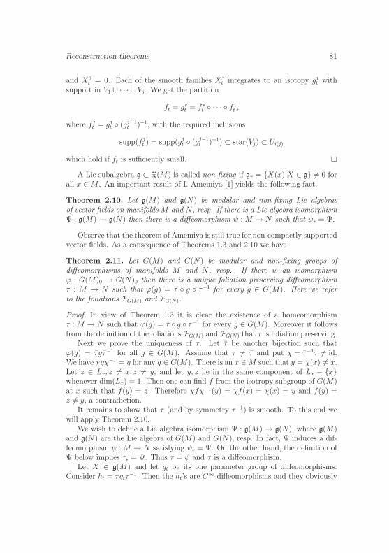
Reconstruction theorems 81
and X0t = 0. Each of the smooth families Xj
t integrates to an isotopy gjt with
support in V1 ∪ · · · ∪ Vj. We get the partition
ft = gst = f s
t · · · f 1t ,
where f jt = gj
t (gj−1t )−1, with the required inclusions
supp(f jt ) = supp(gj
t (gj−1t )−1) ⊂ star(Vj) ⊂ Ui(j)
which hold if ft is sufficiently small.
A Lie subalgebra g ⊂ X(M) is called non-fixing if gx = X(x)|X ∈ g 6= 0 forall x ∈ M . An important result of I. Amemiya [1] yields the following fact.
Theorem 2.10. Let g(M) and g(N) be modular and non-fixing Lie algebrasof vector fields on manifolds M and N , resp. If there is a Lie algebra isomorphismΨ : g(M) → g(N) then there is a diffeomorphism ψ : M → N such that ψ∗ = Ψ.
Observe that the theorem of Amemiya is still true for non-compactly supportedvector fields. As a consequence of Theorems 1.3 and 2.10 we have
Theorem 2.11. Let G(M) and G(N) be modular and non-fixing groups ofdiffeomorphisms of manifolds M and N , resp. If there is an isomorphismϕ : G(M)0 → G(N)0 then there is a unique foliation preserving diffeomorphismτ : M → N such that ϕ(g) = τ g τ−1 for every g ∈ G(M). Here we referto the foliations FG(M) and FG(N).
Proof. In view of Theorem 1.3 it is clear the existence of a homeomorphismτ : M → N such that ϕ(g) = τ g τ−1 for every g ∈ G(M). Moreover it followsfrom the definition of the foliations FG(M) and FG(N) that τ is foliation preserving.
Next we prove the uniqueness of τ . Let τ be another bijection such thatϕ(g) = τ gτ−1 for all g ∈ G(M). Assume that τ 6= τ and put χ = τ−1τ 6= id.We have χgχ−1 = g for any g ∈ G(M). There is an x ∈ M such that y = χ(x) 6= x.Let z ∈ Lx, z 6= x, z 6= y, and let y, z lie in the same component of Lx − xwhenever dim(Lx) = 1. Then one can find f from the isotropy subgroup of G(M)at x such that f(y) = z. Therefore χfχ−1(y) = χf(x) = χ(x) = y and f(y) =z 6= y, a contradiction.
It remains to show that τ (and by symmetry τ−1) is smooth. To this end wewill apply Theorem 2.10.
We wish to define a Lie algebra isomorphism Ψ : g(M) → g(N), where g(M)and g(N) are the Lie algebra of G(M) and G(N), resp. In fact, Ψ induces a dif-feomorphism ψ : M → N satisfying ψ∗ = Ψ. On the other hand, the definition ofΨ below implies τ∗ = Ψ. Thus τ = ψ and τ is a diffeomorphism.
Let X ∈ g(M) and let gt be its one parameter group of diffeomorphisms.Consider ht = τgtτ
−1. Then the ht’s are C∞-diffeomorphisms and they obviously
82 Kowalik, Michalik, Rybicki
satisfy ht+s = hths and h0 = id. Since the action of R on N by (t, x) 7→ ht(x) iscontinuous, in view of a well known theorem of Bochner and Montgomery [4], itis C∞-smooth in both variables. Therefore, it is a one parameter transformationgroup of an element of X(N), say Ψ(X).
Then we have the following equality
(2.2) (Ψ(X)u) τ = X(u τ) ∀u ∈ C∞(N), ∀X ∈ g(M).
This implies also that the right hand side of (2.2) is meaningful for any u andX. In fact, let gt and ht = τgtτ
−1 be the one-parameter transformation groupsof X and Ψ(X), resp. Then (u τ gt)(x) = (u ht τ)(x) for any x ∈ M andthe derivative d
dt(u τ gt)(x)|t=0 exists. Therefore
X(u τ) =d
dt(u τ gt)|t=0 =
d
dt(u ht)|t=0 τ = (Ψ(X)u) τ.
By iterating the above we have also (Ψ(X1)Ψ(X2)u) τ = X1(X2(u τ)).It follows easily from the above equalities that Ψ is a homomorphism. By
uniqueness, ϕ−1 must determine the homeomorphism τ−1. Consequently, the re-spective mapping from g(N) to g(M) is the inverse of Ψ. Thus Ψ is a Lie algebraisomorphism. This completes the proof.
Corollary 2.12. Let FM and FN be foliations on manifolds M and N , resp.If there is an isomorphism ϕ : Diff∞(M,FM)0 → Diff∞(N,FN)0 then there isa foliation preserving diffeomorphism τ : M → N such that ϕ(g) = τ g τ−1 forevery g ∈ Diff∞(M,FM)0.
Conjecture 2.13. By a standard argument using approximation theorems (cf. [6])one has Diffr(Rn)0 = Diffr(Rn)c, where 1 ≤ r ≤ ∞. Now, let 0 < k < n andlet Fn−k be a foliation on Rn−k with L0 = 0. Then F = Rk × LL∈Fn−k
isa foliation on Rn. Note that in light of a splitting theorem by P. Dazord [5] everyfoliation on a manifold assumes locally this form.
Now our conjecture is that Diffr(Rn,F)0 = Diffr(Rn,F)c in view of a possible“foliated” adaptation of the proof of an approximation theorem (this is beyond thescope of this note). As a consequence we would obtain the factorization propertyand the reconstruction theorem for Diffr(Rn,F)c; that is, we could detect from thealgebraic structure of Diffr(Rn,F)c the dimension k and the foliation F .
3 Hamiltonian group of a Poisson manifold
The reconstruction problem in case of Poisson structures has been studied byone of us in [14] but here we use a different definition of the Hamiltonian group(by using regularity) and the resulting group is possibly larger and more naturalthan that in [14].
Reconstruction theorems 83
Poisson structures are nontransitive generalizations of symplectic structures.A Poisson structure on a manifold M can be introduced by a 2-vector Λ on Msuch that [Λ, Λ] = 0, where [., .] is the Schouten-Nijenhuis bracket (see [17]).In general, the rank of Λx varies but it is even everywhere. The ring of the realsmooth functions on M , C∞(M), admits a Lie algebra structure by means of thebracket
(3.1) u, v = Λ(du, dv) for any u, v ∈ C∞(M)
and every adjoint homomorphism of this bracket is a derivation of C∞(M), thatis the Leibniz rule is satisfied
(3.2) u, vw = vu,w+ wu, v.Equivalently, any 2-linear bracket on C∞(M) verifying (3.2) and the Jacobi
rule defines uniquely a Poisson structure Λ by (3.1).We have the ‘sharp’ bundle homomorphism associated with Λ
] : Ω1(M) → X(M), σ(ρ]) = Λ(ρ, σ),
for any 1-forms ρ, σ ∈ Ω1(M), where ρ] = ](ρ). In the case where Λ is nonde-generate (i.e. rank(Λ) = dim(M)), ] is an isomorphism and we get a symplecticstructure. In general, the distribution ](T ∗
xM), x ∈ M , integrates to a generalizedfoliation F(Λ) such that Λ restricted to any leaf induces a symplectic structure.The symplectic form living on L ∈ F(Λ) will be denoted by ωΛ
L .A smooth mapping f of (M, Λ) into itself is called a Poisson morphism if
u f, v f = u, v f for any u, v ∈ C∞(M). Let Diff∞(M, Λ) be the groupof all Poisson diffeomorphisms of (M, Λ) which are leaf preserving with respectto F(Λ). We will show that Diff∞(M, Λ)c is a regular group.
Recall that a vector field X is an infinitesimal automorphism of (M, Λ) if[Λ, X] = 0, that is if LXΛ = 0, where L is the Lie derivative. By X(M, Λ)c wedenote the Lie algebra of all infinitesimal automorphisms of (M, Λ) with com-pact support and tangent to F(Λ). Next, let X∗(M, Λ) be the ideal of X(M, Λ)of all Hamiltonian vector fields, i.e. X ∈ X∗(M, Λ) iff there exists a compactlysupported u ∈ C∞(M) such that X = [Λ, u] or, equivalently, X = (du)]. We havethe inclusion [X(M, Λ), X(M, Λ)] ⊂ X∗(M, Λ) as a consequence of the equality[X1, X2] = [Λ, u], where u is defined by u(x) = ι(X1(x) ∧X2(x))ωΛ
Lx(cf. [9]) .
Proposition 3.1. Let (M, Λ) be an arbitrary Poisson manifold. Suppose that ft
is a compactly supported smooth path with f0 = id and Xt is the correspondingpath in X(M)c given by (2.1). Then ft ∈ Diff∞(M, Λ)0 for each t if and onlyif Xt ∈ X(M, Λ)c for each t.
Proof. By restricting ft to a leaf L and using the equality
∂
∂t(f ∗t ωt) = f ∗t
(Lft
ωt +∂
∂tωt
)
84 Kowalik, Michalik, Rybicki
we have
d
dtf ∗t ωΛ
L = f ∗t (LXtωΛL) = f ∗t (ι(Xt)dωΛ
L + d(ι(Xt)ωΛL)) = f ∗t d(ι(Xt)ω
ΛL).
It follows that the claim is true on any leaf, and consequently so is on M .
A smooth path satisfying Proposition 3.1 is called a Poisson isotopy. A Pois-son isotopy ft is Hamiltonian if the corresponding Xt ∈ X∗(M, Λ)c for each t.A diffeomorphism f of (M, Λ) is called Hamiltonian if there exists a Hamilto-nian isotopy ft such that f0 = id and f1 = f . The totality of all Hamiltoniandiffeomorphisms is denoted by H(M, Λ). It is obvious that H(M, Λ)0 = H(M, Λ).
Proposition 3.2. H(M, Λ) is a normal subgroup of Diff∞(M, Λ)c. Moreover,H(M, Λ) is a regular group with Lie algebra X∗(M, Λ)c.
Proof. First we show that H(M, Λ) satisfies the group axioms. Let ft, gt beHamiltonian isotopies, that is ft = (dut)
], gt = (dvt)] for some smooth families
of C∞-functions ut and vt. Then ft gt is still a Hamiltonian isotopy with thecorresponding smooth path in X∗(M, Λ) being (d(ut + vt f−1
t ))], (cf. [8]). Fur-thermore, we have that f−1
t is Hamiltonian as well with the corresponding smoothpath (d(−ut ft))
]. Therefore H(M, Λ) is a group.Next, if ft is a Hamiltonian isotopy as above and g is a Poisson diffeomorphism
then g−1ftg is also Hamiltonian with the corresponding smooth path (d(utg))].This means that H(M, Λ) is a normal subgroup of Diff∞(M, Λ)c. The secondassertion is trivial.
Lemma 3.3. Let X ∈ X∗(M, Λ)c with supp(X) ⊂ ⋃ki=1 Ui, where the Ui are
open. Then there is a decomposition X = X1 + · · ·+Xk such that Xi ∈ X∗(M, Λ)c
and supp(Xi) ⊂ Ui. The same is true for smooth curves in X∗(M, Λ)c insteadof elements of X∗(M, Λ)c.
The proof is a consequence of the definition of X∗(M, Λ). Although X∗(M, Λ)c
is not modular, Lemma 3.3 combined with [10], chapter X, enable us to prove thefollowing analogue of Theorem 2.10.
Theorem 3.4. Let (M, ΛM) and (N, ΛN) be Poisson manifolds with no leavesof dimension zero. If there is a Lie algebra isomorphism Ψ : X∗(M, ΛM)c →X∗(N, ΛN)c then there is a foliation preserving diffeomorphism ψ : M → N suchthat ψ∗ = Ψ and ψ∗ΛM = µΛN for some nowhere vanishing function µ ∈ C∞(M)which is constant on leaves.
Another consequence of Lemma 3.3 is the fragmentation property forH(M, Λ).
Proposition 3.5. Let f ∈ H(M, Λ) and M =⋃k
i=1 Ui, where the Ui are openballs. Then there exist fj ∈ H(M, Λ), j = 1, . . . , l, with f = f1 . . . fl such thatsupp(fj) ⊂ Ui(j) for all j. The same is true for isotopies in H(M, Λ).
Reconstruction theorems 85
The proof exploits the correspondence between isotopies in H(M, Λ) andsmooth curves in X∗(M, Λ)c given by (2.1) and is similar to that of Proposition2.9.
Theorem 3.6. Let (M, ΛM) and (N, ΛN) be Poisson manifolds with no leavesof dimension 0. If there is an isomorphism ϕ : H(M,FM) → H(N,FN) thenthere is a unique foliation preserving diffeomorphism τ : M → N such that ϕ(g) =τ g τ−1 for every g ∈ H(M,FM) and τ∗ΛM = µΛN for some nowhere vanishingfunction µ ∈ C∞(M) which is constant on leaves.
Proof. The existence of τ is an immediate consequence of Theorem 1.3 and Propo-sition 3.5. The proof of the uniqueness of τ is analogous to that in the proofof Theorem 2.11. In the remaining part of the proof we follow the proof of Theo-rem 2.11 and we use Theorem 3.4.
The following fact can be proved in a “traditional” way ([2], [13]), but here isa consequence of the above results and Theorem 1.3 in [3].
Corollary 3.7. Let (M, ωM) and (N,ωN) be symplectic manifolds and letDiff∞(M, ωM) and Diff∞(M, ωN) be the corresponding symplectomorphism groups.If there is an isomorphism ϕ : Diff∞(M, ωM) → Diff∞(N, ωN) then there is a dif-feomorphism τ : M → N such that ϕ(g) = τ g τ−1 for every g ∈ Diff∞(M, ωM)and τ ∗ωN = CωM for some constant C.
A possible reconstruction theorem for the group of Poisson diffeomorphisms(even if the Poisson structure is regular) is still an open and probably difficultproblem.
References
[1] I.Amemiya, Lie algebra of vector fields and complex structure, J. Math. Soc.Japan 27 (1975), 545-549.
[2] A.Banyaga, The structure of classical diffeomorphism groups, Mathematicsand its Applications, 400, Kluwer Academic Publishers Group, Dordrecht,1997.
[3] E.Ben Ami and M.Rubin, On the reconstruction problem of factorizable home-omorphism groups and foliated manifolds , preprint.
[4] S.Bochner, D.Montgomery, Groups of differentiable and real or complex an-alytic transformations, Ann. Math. 46 (1945), 685-694.
[5] P.Dazord, Feuilletages a singularites. Nederl. Akad. Wetensch. Indag. Math.47 (1985), no. 1, 21–39.
86 Kowalik, Michalik, Rybicki
[6] M.W.Hirsch, Differential topology, Springer-Verlag, New York, 1976.
[7] F.Klein, Erlangen programm, Math. Ann. 43 (1893).
[8] A.Kriegl, P.W.Michor, The Convenient Setting of Global Analysis, Mathe-matical Surveys and Monographs, vol.53, American Mathematical Society,1997.
[9] A.Lichnerowicz, Les varietes de Poisson et leur algebres de Lie associees,J. Diff. Geometry 12 (1977), 253-300.
[10] H.Omori, Infinite dimensional Lie transformation groups, Lecture Notes inMath. 427, Springer-Verlag 1974.
[11] M.Rubin, On the reconstruction of topological spaces from their groupsof homeomorphisms, Trans.Amer.Math. Soc., 312 (1989), 487-537.
[12] M.Rubin, Locally moving groups and reconstruction problems , OrderedGroups and Infinite Permutation Groups Math. Appl. 354, Kluwer Acad.Publ. Dordrecht, (1996), 121-151.
[13] T.Rybicki, Isomorphisms between groups of diffeomorphisms, Proc. Amer.Math. Soc. 123(1995), 303-310.
[14] T.Rybicki, On automorphisms of a Poisson manifold, Soochow J. Math.23(1997), 329-337.
[15] P.Stefan, Accessible sets, orbits and foliations with singularities, Proc.London Math. Soc. 29(1974), 699-713.
[16] P.Stefan, Integrability of systems of vectorfields, London Math. Soc. (2)21(1980), 544-556.
[17] I.Vaisman, Lectures on the Geometry of Poisson Manifolds, Progress in Math.118, Birkhauser 1994.
Agnieszka Kowalike-mail: [email protected] Michalike-mail: [email protected] Rybickie-mail: [email protected]
Faculty of Applied MathematicsAGH University of Science and Technologyal. Mickiewicza 3030-059 KrakowPoland
Travaux mathematiques, Volume 18 (2008), 87–92, c© Universite du Luxembourg
Bernoulli-Taylor formula in the case of Q-umbral Calculus 1
by Ewa Krot-Sieniawska
Abstract
In this note we derive the Q-difference Bernoulli-Taylor formula withthe rest term of the Cauchy form by the Viskov’s method [1]. This isan extension of technique presented in [5, 6, 7] by the use of Q-extendedKwasniewski’s ∗ψ-product [3, 4]. The main theorems of Q-umbral cal-culus were given by G. Markowsky in 1968 (see [2]) and extended byA.K.Kwasniewski [3, 4].
Mathematics Subject Classification. 17B01, 17B35, 33C45.
Keywords. Generalized differential operator, ∗Q-product, Q-integral.
1 Introduction - Q-umbral calculus
We shall denote by P the algebra of polynomials over the field F of characteristiczero.
Let us consider a one parameter family F of sequences. Then a sequence ψ iscalled admissible ([3, 4]) if ψ ∈ F . Where
F = Ψ : R ⊃ [a, b]; q ∈ [a, b] : Ψ(q) : Z→ F; Ψ0(q) = 1, Ψn(q) 6= 0,
Ψ−n(q) = 0, n ∈ N.Now let us to introduce the Ψ-notation [3, 4]:
nψ = Ψn−1(q)Ψ−1n (q);
nψ! = nψ(n− 1)ψ · · · 2ψ1ψ = Ψ−1n (q),
nkψ = nψ(n− 1)ψ · · · (n− k + 1)ψ,
(n
k
)
ψ
=nk
ψ
kψ!,
expψy =∞∑
k=0
yk
kψ!.
1Received: October 31, 2007
88 Ewa Krot-Sieniawska
Definition 1.1. [2, 3] Let Q be a linear map Q : P → P such that:
∀p∈P deg(Qp) = (deg p)− 1,
deg p=−1 means p=const=0. Then Q is called a generalized differential operator[2].
Definition 1.2. [2] A normal sequence of polynomials qn(x)n≥0 has the follow-ing properties:
(a) ∀n≥0 deg qn(x) = n;
(b) ∀x∈F q0(x) = 1 ;
(c) ∀n≥1 qn(0) = 0 .
Definition 1.3. [2, 3] Let qn(x)n≥0 be the normal sequence of polynomials.Then we call it the ψ-basic sequence of the generalized differential operator Q (orQ−ψ−basic sequence) if:
∀n≥0 Qqn(x) = nψqn−1(x).
In [2] it is shown that once a differential operator Q is given a unique ψ-basicpolynomial sequence is determined and the other way round: given a normalsequence qn(x)n≥0 there exists a uniquely determined generalized differentialoperator Q.
Definition 1.4. [2, 3] The xQ-operator (Q-multiplication operator, the operatordual to Q ) is the linear map xQ : P → P such that:
∀n≥0 xQqn(x) =n + 1
(n + 1)ψ
qn+1(x).
Note that: [Q, xQ] = id.
Definition 1.5. [3] Let qn(x)n≥0 be a Q−ψ−basic sequence. Let
Eyq (Q) = Ey(Q) = expQ, ψyQ =
∞∑
k=0
qk(y)Qk
kψ!.
Eyq (Q) = Ey(Q) is called the Q−ψ−generalized translation operator.
As was announced in [5, 7], the notion of Kwasniewski’s ∗ψ product and itsproperties presented in [3] can be easily Q-extended as follows.
Bernoulli-Taylor formula in the case of Q-umbral Calculus 89
Definition 1.6. [3]
x ∗Q qn(x) = xQ(qn(x)) =n + 1
(n + 1)ψ
qn+1(x), n ≥ 0
xn ∗Q qn(x) = (xnQ)(q1(x)) =
(n + 1)!
(n + 1)ψ!qn+1(x), n ≥ 0
Therefore
x ∗Q α1 = x ∗Q αq0(x) = xQ(αq0(x)) = αxQ(q0(x)) = αx ∗Q 1
andf(x) ∗Q qn(x) = f(xQ)qn(x)
for every formal series f (f ∈ F[[x]]).
Definition 1.7. According to definition above and [3] we can define Q-powers ofx by recurrence relation:
x0∗Q = 1 = q0(x)
xn∗Q = x ∗Q (x(n−1)∗Q) = xQ(x(n−1)∗Q).
It is easy to show that:
xn∗Q = x ∗Q x ∗Q . . . ∗Q 1 =n!
nψ!qn(x), n ≥ 0.
Also note that:
xn∗Q ∗Q xk∗Q =n!
nψ!qk+n(x)
and
xk∗Q ∗Q xn∗Q =k!
kψ!qk+n(x)
so in general i.e. for arbitrary admissible ψ and for every qn(x)n≥0 it is non-commutative.
Due to definition above one can prove the following Q-extended properties ofKwasniewski’s ∗ψ product [3, 4].
Proposition 1.8. Let f, g be formal series, (f, g ∈ F[[x]]). Then for ∗Q definedabove holds:
(a) Qxn∗Q = nx(n−1)∗Q , n ≥ 0;
(b) expQ,ψ[αx] = expαxQ1, where expQ, ψαx =∑
k≥0
qk(x)αk
kψ !;
(c) Q(xk ∗Q xn∗Q) = (Dxk) ∗Q xn∗Q + xk ∗Q (Qxn∗Q);
90 Ewa Krot-Sieniawska
(d) Q(f ∗Q g) = (Df) ∗Q g + f ∗Q (Qg), (Q-Leibnitz rule);
(e) f(xQ)g(xQ)1 = f(x) ∗Q g; g(x) = g(xQ)1.
According to [2, 3], let us to define Q-integration operator which is a rightinverse operation to generalized differential operator Q i.e.:
Q ∫
dQt = id.
Definition 1.9. We define Q-integral as a linear operator such that∫
qn(x)dQx =1
(n + 1)ψ
qn+1(x); n ≥ 0.
Proposition 1.10.
(a) Q ∫ x
αf(t)dQt = f(x);
(b)∫ x
α(Qf)(t)dQt = f(x)− f(α);
(c) formula for integration ”per partes” :
∫ β
α
(f ∗Q Qg)(x)dQx = [(f ∗Q g)(x)]βα −∫ β
α
((Df) ∗Q g)(x)dQx.
2 Q-umbral calculus Bernoulli-Taylor formula
In [1] O.V.Viskov establishes the following identity
(2.1) p
n∑
k=0
(−q)kpk
k!=
(−q)npn+1
n!
what he calls the Bernoulli identity. Here p, q stand for linear operators satisfyingcondition:
(2.2) [p, q] = pq − qp = id.
Now let p and q be as below:
p = Q, q = xQ − y, y ∈ F.
From definition (1.4) we have [Q, xQ − y] = id. After substitution into (2.1) weget:
Q
n∑
k=0
(y − xQ)kQk
k!=
(y − xQ)nQn+1
n!.
Bernoulli-Taylor formula in the case of Q-umbral Calculus 91
Now let us apply it to any polynomial (formal series) f :
Q
n∑
k=0
(y − xQ)k(Qkf)(t)
k!=
(y − xQ)n(Qn+1f)(t)
n!.
Now using definitions (1.6) and (1.7) of ∗Q-product we get:
Q
n∑
k=0
(y − x)k∗Q ∗Q (Qkf)(t)
k!=
(y − x)n∗Q ∗Q (Qn+1f)(t)
n!.
After integration∫ x
ydQt using proposition (1.2) it gives Q-difference calculus
Bernoulli-Taylor formula of the form:
(2.3) f(x) =n∑
k=0
1
k!(x− y)k∗Q ∗Q (Qkf)(y) + Rn+1(x)
where Rn+1 stands for the rest term of the Cauchy type :
(2.4) Rn+1(x) =1
n!
∫ x
y
(x− t)n∗Q ∗Q (Qn+1f)(t)dψt.
3 Special cases
1. An example of generalized differential operator is Q ≡ ∂ψ. Then qn = xn
and ∂ψxn = nψxn−1 for an admissible ψ. ∂ψ is called ψ-derivative. Then
also xQ ≡ xψ and xψxn = (n+1)(n+1)ψ
xn+1 and [∂ψ, xψ] = id. In this case we get
∂ψ -difference calculus Bernoulli-Taylor formula presented in [5, 6, 7] of theform
f(x) =n∑
k=0
1
k!(x− α)k∗ψ ∗ψ (∂k
ψf)(α) + Rn+1(x)
with
Rn+1(x) =1
n!
∫ x
α
(x− t)n∗ψ ∗ψ (∂n+1ψ f)(t)dψt.
In [3] there is given a condition for the case Q = Q(∂ψ) for some admissibleψ, (see Section 2, Observation 2.1).
2. For Q = ∂ψ, qn(x) = xn, n ≥ 0 the choice ψn(q) = 1[R(qn)]!
, R(x) = 1−x1−q
gives the well known q-factorial nq! = nq(n − 1)q . . . 2q1q, for nq = 1 + q +q2 + . . . + qn−1. Then ∂ψ = ∂q becomes the well known Jackson’s derivative∂q:
(∂qf)(x) =f(x)− f(qx)
(1− q)x
The ∂q-difference version of the Bernoulli-Taylor formula was given in [5] bythe use of ∗q-product.
92 Ewa Krot-Sieniawska
3. By the choice Q ≡ D ≡ ddx
, qn(x) = xn and ψn = 1n!
after substitution to(2.3), (2.4) we get the classical Bernoulli-Taylor formula of the form:
f(x) =n∑
k=0
(x− α)k
k!f (k)(α) +
∫ x
α
(x− t)n
n!fn+1(t)dt
where f (k)(α) = (Dkf)(α).
Acknowledgements. I would like to thank Professor A. Krzysztof Kwasniewskifor his very helpful comments, suggestions, improvements and corrections of thisnote.
References
[1] O.V. Viskov, Noncommutative aproach to Classical Problems of Analysis,Trudy matiematicz’eskovo Instituta AN SSSR 177 (1986), pp.21, in russian.
[2] G. Markowsky, Differential operators and the theory of binomial enumeration,J. Math. Anal.Appl. 63 (1978), pp.145-155.
[3] A.K. Kwasniewski, Main theorems of extended finite operator calculus, Inte-gral Transforms and Special Functions Vol. 14 No 6 (2003), pp.499-516.
[4] A.K. Kwasniewski, Extended finite operator calculus - an example of alge-braization of analysis, Bulletin of the Allahabad Mathematical Society Vol20 2005 pp. 1-24.
[5] A.K. Kwasniewski, Bernoulli-Taylor formula of ψ-umbral dif-ference calculus, Faculty of Mathematics, Univesity of ÃLodz,http://www.math.uni.lodz.pl/main/polish/preprints/.
[6] A.K. Kwasniewski, On ψ-umbral difference calculus Bernoulli-Taylor formulawith a Cauchy-type remainder, Bulletin de la Societe des Sciences et desLettres de ÃLodz Vol.54, Serie: Recherches sur les Deformations Vol. 44 (2004),pp. 21-29.
[7] A.K. Kwasniewski, More on Bernoulli-Taylor formula for extended umbralcalculus, Advances in Applied Clifford Algebras, Vol. 16 (1) 2006, pp. 29-39.
Ewa Krot-SieniawskaInstitute of Computer Science, University in BiaÃlystokPL-15-887 BiaÃlystok, ul.Sosnowa 64, POLANDe-mail: [email protected]
Travaux mathematiques, Volume 18 (2008), 93–101, c© Universite du Luxembourg
On the pseudoharmonic functions1
by Iryna Yurchuk
Abstract
We will obtain the conditions for pseudoharmonic functions defined ona disk to be topologically equivalent in term of their invariant that is afinite connected graph with a strict partial order on vertices. The inverseproblem of the realization of a graph as a combinatorial invariant of suchfunctions will be solved.
1 Introduction
In [1, 2, 3, 9] the conditions for a topological equivalence of functions, flows,and other structures on manifolds were obtained. Almost all of such solutionsare formulated by using their invariants which are some combinatorial objects(graphs, chord diagrams, shakes etc.) For example in [2] the authors constructedspin graphs that were used for the classification of Morse-Smale flows on closedsurfaces. In this note we use the so called combinatorial diagrams (being graphswith additional data) for the classification of pseudoharmonic functions on 2-disk.
Let D2 ⊂ C be a oriented closed 2−disk and f : D2 → R be a pseudoharmonicfunction. Recall that a function f is pseudoharmonic if there is a preserving orien-tation homeomorphism ϕ of a domain D2 onto itself such that f ϕ is harmonic.
Let us characterize all types of points of IntD2 and ∂D2.A point z0 ∈ IntD2 is called a regular point of f if there is a U(z0) in which
f equals to f = Rez + f(z0), otherwise z0 is critical.A point z0 ∈ ∂D2 is called a boundary regular point of f if there exist U(z0) ∈
D2 and a homeomorphism h : U → D2+ of it onto a semidisk D2
+ = D2 ∩ (R ×[0, +∞)) such that a function h f h−1 : D2
+ → R equals to Rez + f(z0).Points of ∂D2 that are neither regular nor isolated points of their level curves
will be called boundary critical.A value c of f is called critical (regular) if the connected components of level
curves of f−1(c) contain critical points (don’t contain critical points and are home-omorphic to a disjoint union of segments that intersect the ∂D2 in their endpoints).
Definition 1.1. A value c of f is semiregular if it is neither regular nor critical.
1Received: October 31, 2007
94 Iryna Yurchuk
It is known that the level curves of a critical value of a pseudoharmonic functionare trees (in general, a disjoint union of trees) [4].
By f |∂D2 we denote a restriction of f on the boundary ∂D2. We will beinterested in a case when f |∂D2 has a finite number of local extrema. In otherwords, the pseudoharmonic function defined on D2 ⊂ C is a continuous functionsatisfying the following conditions [4, 5, 6, 8]:
• f |∂D2 is a continuous function with a finite number of local extrema;
• f has a finite number of critical points in the interior of a disk and each ofthem is a saddle point (in the neighborhood of them the function f has arepresentation like f = Rezn + const, n ≥ 2, where z = x + iy).
At first we will construct its combinatorial invariant (called a combinatorial dia-gram) and formulate a necessary and sufficient condition of a topological equiva-lence of such function. After that we will be interested in the converse problem.Suppose we are given a graph, to which conditions it should satisfy to be a com-binatorial invariant of a pseudoharmonic function.
Let us recall some definitions. We will say that f, g : D2 → R are topologicallyequivalent if there exist preserving orientation homeomorphisms h1 : D2 → D2
and h2 : R→ R such that f = h−12 g h1.
By a graph G we mean a topological graph (i.e., a CW - complex with 0 and1 – cells, where 0−cells are its vertices and 1− cells are its edges). Let T be a tree(i.e., a CW−complex such that it does not contain cycles). Denote by V the setof its vertices and by Vter(T ) the subset of V consisting of all terminal vertices.A disjoint union of trees is called a forest and denoted by F =
⋃i
Ψi, where every
Ψi is a tree. By a path P (vi, vk) which connects vertices vi and vk of G we meana sequence of edges ej such that each of them belongs to it once. It is knownthat for any two vertices of a tree there is a unique path connecting them. Twovertices of a graph are adjacent if they are the ends of the same edge. A graph Gis embedded into R2 if there exists a bijection φ : G → R2 such that two pointsφ(x) and φ(y) are joined by a segment iff x and y are joined by an edge of G andno two distinct open segments have a point in common.
2 Theorem of a topological equivalence
Since a disk is a manifold with a boundary and the problem of a construction ofa invariant of such manifolds is unsolved we need to obtain a special structure.
First construct the Kronrod-Reeb graph (ΓK−R) of f |∂D2 . ΓK−R(f |∂D2) isisomorphic to a circle with even number of vertices. Then, we add to ΓK−R(f |∂D2)
collections of connected components f−1(ai) ⊆ f−1(ai) and f−1(ci) ⊆ f−1(ci)
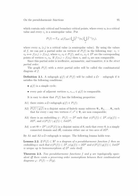
On the pseudoharmonic functions 95
which contain only critical and boundary critical points, where every ai is a criticalvalue and every cj is a semiregular value. Put
P (f) = ΓK−R(f |∂D2)⋃i
f−1(ai)⋃j
f−1(cj),
where every ai (cj) is a critical value (a semiregular value). By using the valuesof f , we can put a partial order on vertices of P (f) in the following way: v1 >v2 ⇐⇒ f(x1) > f(x2), where v1, v2 ∈ P (f), and x1, x2 ∈ D2 are the correspondingpoints of vertices v1, v2. If f(x1) = f(x2) then v1 and v2 are non comparable.
Since this partial order is irreflexive, asymmetric, and transitive, it is the strictpartial order.
The graph P (f) with a strict partial order will be called the combinatorialdiagram of f .
Definition 2.1. A subgraph q(f) of P (f) will be called a Cr – subgraph if itsatisfies the following conditions:
• q(f) is a simple cycle;
• every pair of adjacent vertices vi, vi+1 ∈ q(f) is comparable.
It is easy to show that P (f) has the following properties:
A1) there exists a Cr-subgraph q(f) ∈ P (f);
A2) P (f) \ q(f) is a disjoint union of finitely many subtrees Ψ1, Ψ2, . . . , Ψn suchthat for every i any two vertices v′, v′′ ∈ Ψi are non comparable;
A3) there is an embedding ψ : P (f) → D2 such that ψ(P (f)) ⊂ D2, ψ(q(f)) =∂D2, and ψ(P (f) \ q(f)) ⊂ IntD2;
A4) a set Θ = D2\ψ(P (f)) is a disjoint union of θi such that every θi is a simplyconnected domain and ∂θi contains either one or two arcs of ∂D2.
By A1 and A2 a Cr-subgraph is unique. The following lemma holds true.
Lemma 2.2. If P (f) ⊂ R3 is a diagram of a pseudoharmonic function f then anembedding ψ such that ψ(P (f)) ⊂ D2, ψ(q(f)) = ∂D2 and ψ(P (f)\q(f)) ⊂ IntD2
is unique up to homeomorphism of D2 onto itself.
Theorem 2.3. Two pseudoharmonic functions f and g are topologically equiv-alent iff there exists a preserving order isomorphism between their combinatorialdiagrams ϕ : P (f) → P (g).
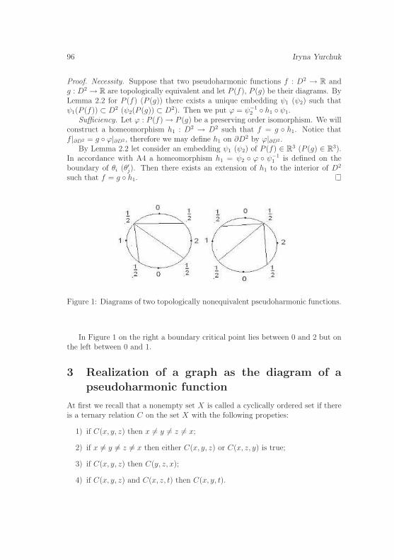
96 Iryna Yurchuk
Proof. Necessity. Suppose that two pseudoharmonic functions f : D2 → R andg : D2 → R are topologically equivalent and let P (f), P (g) be their diagrams. ByLemma 2.2 for P (f) (P (g)) there exists a unique embedding ψ1 (ψ2) such thatψ1(P (f)) ⊂ D2 (ψ2(P (g)) ⊂ D2). Then we put ϕ = ψ−1
2 h1 ψ1.Sufficiency. Let ϕ : P (f) → P (g) be a preserving order isomorphism. We will
construct a homeomorphism h1 : D2 → D2 such that f = g h1. Notice thatf |∂D2 = g ϕ|∂D2 , therefore we may define h1 on ∂D2 by ϕ|∂D2 .
By Lemma 2.2 let consider an embedding ψ1 (ψ2) of P (f) ∈ R3 (P (g) ∈ R3).In accordance with A4 a homeomorphism h1 = ψ2 ϕ ψ−1
1 is defined on theboundary of θi (θ′j). Then there exists an extension of h1 to the interior of D2
such that f = g h1.
Figure 1: Diagrams of two topologically nonequivalent pseudoharmonic functions.
In Figure 1 on the right a boundary critical point lies between 0 and 2 but onthe left between 0 and 1.
3 Realization of a graph as the diagram of a
pseudoharmonic function
At first we recall that a nonempty set X is called a cyclically ordered set if thereis a ternary relation C on the set X with the following propeties:
1) if C(x, y, z) then x 6= y 6= z 6= x;
2) if x 6= y 6= z 6= x then either C(x, y, z) or C(x, z, y) is true;
3) if C(x, y, z) then C(y, z, x);
4) if C(x, y, z) and C(x, z, t) then C(x, y, t).

On the pseudoharmonic functions 97
Two elements are neighboring with respect to a fixed cyclic order C if for any x 6=x′, x′′ we have either C(x′, x′′, x) or C(x′′, x′, x). Let fix a subset V ∗ of vertices of atree T such that Vter(T ) ⊆ V ∗ ⊆ V and put a cyclic order on them. The notationC(vj1 , vj2 , ..., vjk
) means that C(vj1 , vj2 , ..., vjk) = C(vjk
, vj1 , vj2 , ..., vjk−1) = . . . =
C(vj2 , ..., vjk, vj1), where vji
6= vjk, k 6= i, vji
∈ V ∗.
Definition 3.1. A tree T with a fixed cyclic order of vertices vi ∈ V ∗ is called a D-planar if there exists an embedding ϕ such that ϕ(T ) ⊂ D2, ϕ(V ∗) ⊂ ∂D2, ϕ(T \V ∗) ⊂ IntD2, C(vj1 , vj2 , ..., vjk
)= C(ϕ(vj1), ϕ(vj2), ..., ϕ(vjk)), where a cyclic order
C(ϕ(vj1), ϕ(vj2), ..., ϕ(vjk)) is generated by the orientation of ∂D2 and Vter(T ) ⊆
V ∗ ⊆ V .
The next theorem is a criteria of the D-planarity of a tree.
Theorem 3.2. If ]V ∗ = 2 then a tree T is a D-planar.If ]V ∗ ≥ 3 then the D-planarity of a tree T is equivalent to the following
condition that has to be satisfied: for every edge e there are exactly two paths inT such that they pass through an edge e and connect adjacent vertices of V ∗.
We leave the proof to the reader.
12
3
4 5 6
7
12
34
5 6 7
12
3
45
6
7
1
2
3
4
5 6
7
Figure 2: On the right a tree is not a D– planar.
Let G be a finite connected graph with a strict partial order and every of itsvertex has a degree greater than 1.
Definition 3.3. A simple cycle γ ⊂ G will be called a Cr – cycle if every pair ofadjacent vertices of γ are comparable.
98 Iryna Yurchuk
Suppose that for a graph G the following conditions hold:
C1) a graph G has a unique Cr-cycle γ;;
C2) G \ γ = F =k⋃
i=1
Ψi where F is a forest such that
• any two vertices vj and vk of every connected component Ψi ⊂ F arenon comparable;
• for any vertex v ∈ G \ γ it is true that deg(v) = 2s ≥ 4;
C3) Condition on a strict order for Cr – cycle γ:
for any vertex v of γ and its adjacent vertices v1 and v2 such that v1, v2 ∈ γone of the following conditions holds true:
• if deg(v) = 2 then deg(v1) > 2, deg(v2) > 2 and there exists a uniqueindex i such that v1, v2 ∈ Ψi;
• if deg(v) = 2s > 2 (deg(v) = 2s + 1) then v1 ≶ v ≷ v2 (v1 ≶ v ≶ v2);
C4) Condition on a strict order for G: if for some vertices of G we have thatv < v′ (v > v′) and v′, v′′ ∈ Ψi ⊆ G \ γ then v < v′′ (v > v′′);.
By C2 there exists a nonempty subset of vertices V ∗ of F such that V ∗ ∈ γ. It isclear that a subset V ∗ of F is divided into subsets V ∗
i such that V ∗ =⋃i
V ∗i and
V ∗i ⊂ Ψi ⊂ F .
Definition 3.4. A graph G ⊂ R3 satisfying C1 and C2 is called a D−planar ifthere exists an embedding ϕ : G → D2 such that ϕ(γ) = ∂D2, ϕ(G \ γ) ⊂ IntD2.
Theorem 3.5. A graph G satisfying C1 and C2 is a D – planar iff every tree Ψi
with a subset of vertices V ∗i that has a cyclic order defined by γ is a D-planar and
for any index m 6= n a set V ∗n belongs to a unique connected component of γ \V ∗
m.
Let v1 and v2 be any two vertices v1, v2 ∈ V ∗i ⊆ Ψi ⊆ G satisfying C1 and C2.
A set γ \ (v1 ∪ v2) consists of a disjoint union of sets γ1 and γ2.
Definition 3.6. A pair of vertices v1, v2 ∈ V ∗i is called boundary if there exists
an index k such that γk does not contain vertices of a set V ∗i and at least one
vertex of V ∗ \ V ∗i belongs to γk, k = 1, 2.
Denoted by ω(v1, v2) a boundary pair and by α a set γk from Definition 3.6.It is clear that for every vertex vi of ω(v1, v2) there exists an adjacent vertex vi
such that vi ∈ α where i = 1, 2.
Definition 3.7. A graph G is called special if the following conditions hold:
On the pseudoharmonic functions 99
S1) G satisfies C1 and C2;
S2) G is a D – planar;
S3) for any boundary pair ω(v1, v2) ∈ V ∗i the pair v1, v2 belongs to a unique set
V ∗k , where V ∗
k ⊂ V ∗ \ V ∗i .
Lemma 3.8. If a graph G is special then the set Θ = D2 \ φ(G) consists of adisjoint union of domains θi such that every ∂θi contains either one or two arcsof a boundary ∂D2, where φ : G → D2 is an embedding such that φ(γ) = ∂D2,φ(G \ γ) ⊂ IntD2.
Definition 3.9. A special graph G is called a ∆ – graph if it satisfies C3.
Let us there are two partial order < and <′ on a set A. We will say that a par-tial order < can be extended to <′ if a map Id : (A,<) → (A,<′) is monotonous.
Theorem 3.10. If graph is a combinatorial diagram of a pseudoharmonic functionf then G is a ∆ – graph.
If a graph G is a ∆ – graph, then a strict partial order on V (G) can be ex-tended to one so that a graph G with new partial order on a set of vertices will beisomorphic to the combinatorial diagram of some pseudoharmonic function f . Astrict partial order of a graph G coincides with a strict partial order of a combi-natorial diagram P (f) of a pseudoharmonic function f iff G satisfies:
if vertices v′, v′′ are non comparable then from v > v′ follows v > v′′ wherev ∈ G, v 6= v′, v 6= v′′.
We briefly give main ideas of a proof.
Proof. Necessity. This follows from A1-A4.Sufficiency. Let G be a ∆ – graph. By Definition 3.7 and Lemma 3.8 there
exists an embedding φ : G → D2 such that φ(γ) = ∂D2, φ(G \ γ) = IntD2, andthe set Θ = D2 \ φ(G) consists of a disjoint union of domains θi such that every∂θi contains either one or two arcs of a boundary ∂D2. For every θi let us definea foliation:
Case 1: Let θk1 ⊂ Θ and ∂θk1 contains one arc Si ⊂ ∂D2. We consider φ−1(Si).Since γ is a Cr – cycle satisfying C3, the set φ−1(Si) consists of two edges e1 ande1 such that they are adjacent to vertex v (its degree equals to 2) and anothertheir end vertices are non comparable. We define a foliation by curves Γi such thatfor any index i it is true that Γi
⋂Si = xi
1 ∪ xi2, lim
i→nΓi = ∂θk1 \ Si, and
⋂i
Γi = ∅,
Γ0 = ∂ε(φ(v)), where xi1 ∈ φ−1(e1), xi
2 ∈ φ−1(e2), ε(φ(v)) is a neighborhood ofφ(v) (Figure 3).
Case 2: Let θk2 ⊂ Θ be such that ∂θk2 contains two boundary arcs Sni⊂ ∂D2
and Smi⊂ ∂D2. We consider φ−1(Sni
) and φ−1(Smi). Since γ is Cr – cycle
satisfying C3, the set φ−1(Sni) (φ−1(Smi
)) consists of an edge e1 (e2) such that its
100 Iryna Yurchuk
Figure 3: A foliation of a domain with one boundary arc.
end vertices are comparable. It is clear that ∂θk1 \ (Sni∪ Smi
) = λ1 ∪ λ2, whereφ−1(λ1) ∈ Ψl, φ−1(λ2) ∈ Ψk. We define a foliation by curves Γi such that for anyindex i it is true that Γi
⋂Sni
= xi1, Γi
⋂Smi
= xi2 and lim
i→nΓi = λ2,
⋂i
Γi = ∅,
Γ0 = λ1, where xi1 ∈ φ−1(e1), xi
2 ∈ φ−1(e2) (Figure 4).
Figure 4: A foliation of a domain with two boundary arcs.
A family of curves Γj is a regular and there exists a continuous functionsuch that this family is the level curves of it [7]. Therefore for every θi there isa continuous function fi. Since θi ∩ θj 6= ∅ and fi(x) = fj(x), where x ∈ θi ∩ θj,there exist a continuous function f such that f |θi
= fi. By C2 all critical pointsof IntD2 are saddle.
Let consider the restriction of f onto ∂D2. The points φ(vi) corresponding tovertices vi such that vi ∈ γ and deg(vi) = 2k are local extrema of it. It is obviousthat there is a finite number of them. By C3 it is easy to prove that after localminima be next a local maxima on ∂D2.
On the pseudoharmonic functions 101
Corollary 3.11. Let G is a ∆ – graph. G satisfies C4 iff a strict partial order ofG coincides with a strict partial order of a combinatorial diagram P (f) of somepseudoharmonic function f corresponding it.
References
[1] Arnold V.I., Bernoulli – Euler updown numbers associated with function sin-gularities, their combinatorics and mathematics, Duke Math. J., 1991, 63. 2,pp. 537-555
[2] Bolsinov A.V., Oshemkov A.A., Sharko V.V., On classification of flows onmanifolds I, Meth. Funct. Anal. Top., 1996, vol. 2, no.2, pp. 51-60
[3] Bolsinov A. V., Fomenko A. T., Exact topological classification of Hamil-tonian flows on smooth two-dimensional surfaces (Russian summary), Zap.Nauchn. Sem. S.-Peterburg, Otdel. Mat. Inst. Steklov, 1996, 235, pp. 22-53
[4] Boothby W.M., The topology of regular curve families with multiple saddlepoints, Amer. J. Math., 1951, 73, pp. 405-438
[5] Jenkins J.A, Morse M., Contour equivalent pseudoharmonic functions andpseudoconjugates, Amer. J. Math., 1952, 74, pp. 23-51
[6] Kaplan W., Topology of level curves of harmonic functions, Trans. Amer.Math. Soc., 1948, vol. 63. 3, pp. 514-522
[7] Kaplan W., Regular Curve - Families Filling the Plane I, Duke Math. J.,1940, vol. 7, pp. 154-184
[8] Morse M., The topology of pseudo-harmonic functions, Duke Math. J., 1946,13, pp. 21-42
[9] Prishlyak A. O., Regular functions on closed three-dimensional manifolds,Dopov. Nats. Akad. Nauk Ukr. Mat. Prirodozn. Tekh. Nauki, 2003, no. 8,pp. 21-24
Iryna YurchukTopology Department, Institute of Mathematics,Ukrainian National Academy of Science,Tereshchenkivska str. 3, 01601 Kyiv, [email protected]

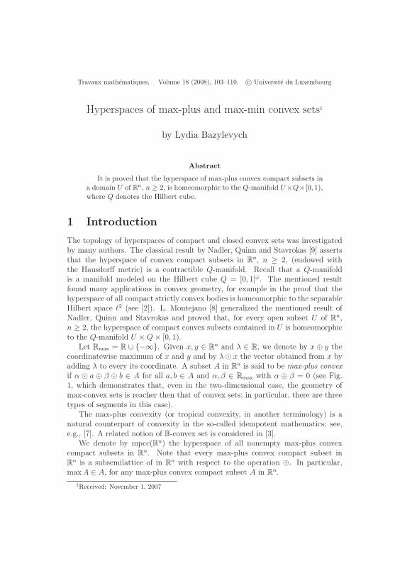
Travaux mathematiques, Volume 18 (2008), 103–110, c© Universite du Luxembourg
Hyperspaces of max-plus and max-min convex sets1
by Lydia Bazylevych
Abstract
It is proved that the hyperspace of max-plus convex compact subsets ina domain U of Rn, n ≥ 2, is homeomorphic to the Q-manifold U×Q×[0, 1),where Q denotes the Hilbert cube.
1 Introduction
The topology of hyperspaces of compact and closed convex sets was investigatedby many authors. The classical result by Nadler, Quinn and Stavrokas [9] assertsthat the hyperspace of convex compact subsets in Rn, n ≥ 2, (endowed withthe Hausdorff metric) is a contractible Q-manifold. Recall that a Q-manifoldis a manifold modeled on the Hilbert cube Q = [0, 1]ω. The mentioned resultfound many applications in convex geometry, for example in the proof that thehyperspace of all compact strictly convex bodies is homeomorphic to the separableHilbert space `2 (see [2]). L. Montejano [8] generalized the mentioned result ofNadler, Quinn and Stavrokas and proved that, for every open subset U of Rn,n ≥ 2, the hyperspace of compact convex subsets contained in U is homeomorphicto the Q-manifold U ×Q× [0, 1).
Let Rmax = R ∪ −∞. Given x, y ∈ Rn and λ ∈ R, we denote by x ⊕ y thecoordinatewise maximum of x and y and by λ¯ x the vector obtained from x byadding λ to every its coordinate. A subset A in Rn is said to be max-plus convexif α ¯ a ⊕ β ¯ b ∈ A for all a, b ∈ A and α, β ∈ Rmax with α ⊕ β = 0 (see Fig.1, which demonstrates that, even in the two-dimensional case, the geometry ofmax-convex sets is reacher then that of convex sets; in particular, there are threetypes of segments in this case).
The max-plus convexity (or tropical convexity, in another terminology) is anatural counterpart of convexity in the so-called idempotent mathematics; see,e.g., [7]. A related notion of B-convex set is considered in [3].
We denote by mpcc(Rn) the hyperspace of all nonempty max-plus convexcompact subsets in Rn. Note that every max-plus convex compact subset inRn is a subsemilattice of in Rn with respect to the operation ⊕. In particular,max A ∈ A, for any max-plus convex compact subset A in Rn.
1Received: November 1, 2007
104 Lydia Bazylevych
q
q
q
q
q
q
¡¡
¡¡
¡¡
¡¡
¡¡
¡¡
¡¡
¡¡
¡
¡¡
¡¡¡
¡¡
¡¡¡
Figure 1: A max-plus convex set and typical segments in the plane
The aim of this paper is to show that there exists a max-plus counterpartof the Montejano theorem. We prove that the hyperspace of max-plus convexcompact sets in an open set U of Rn, n ≥ 2, is the Q-manifold U ×Q× [0, 1).
In order to keep a reasonable length of this publication we only outline theproofs and omit technical details. They will appear elsewhere.
2 Preliminaries
If a ∈ Rn, we write a = (a1, . . . , an). We endow Rn with the L∞-metric d,d(a, b) = maxi |ai − bi|. The set Rmax is endowed with the metric %, %(x, y) =|ex − ey| (convention: e−∞ = 0).
By exp X we denote the set of all nonempty compact subsets of a metric space(X, d). We endow exp X with the Hausdorff metric dH :
dH(A,B) = infε > 0 | A ⊂ Oε(B), B ⊂ Oε(A)(hereafter, Or(C) denotes the r-neighborhood of C ∈ exp X; also, by Or(C)we denote the closed r-neighborhood of C). We denote by max the maximumoperation in Rn. Note that, for any nonempty compact subset A in Rn, theelement max(A) is well-defined.
Lemma 2.1. The maximum map max: mpcc(Rn) → Rn is continuous.
Proof. Suppose that A,B ∈ mpcc(Rn) and dH(A,B) = ε ≥ 0. Let max(A) =(p1, . . . , pn), max(B) = (q1, . . . , qn). Suppose that d(max(A), max(B)) > ε. With-out loss of generality, we may assume that qi > pi + ε, for some i. Then
Hyperspaces of max-plus and max-min convex sets 105
Oqi−pi(max(B)) does not intersect A, whence dH(A,B) ≥ qi − pi > ε. The
obtained contradiction demonstrates that d(max(A), max(B)) ≤ dH(A,B). ThusdH is nonexpanding and therefore continuous.
Note also that max(A) ∈ A, for every A ∈ mpcc(Rn).For any subset U of Rn, by mpcc(U) we denote the set
A ∈ mpcc(Rn) | A ⊂ U.
Recall that a map is said to be proper if the preimage of any compact subsetis compact.
By AR (respectively ANR) we denote the class of absolute (neighborhood)retracts for the class of metrizable spaces.
The following notion is introduced in [6]. A c-structure on a topological spaceX is an assignment to every nonempty finite subset A of X a contractible subspaceF (A) of X such that F (A) ⊂ F (A′) whenever A ⊂ A′. A pair (X,F ), where Fis a c-structure on X is called a c-space. A subset E of X is called an F -set ifF (A) ⊂ E for any finite A ⊂ E. A metric c-space (X, d) is said to be a metricl.c.-space if all the open balls are F -sets and all open r-neighborhoods of F -setsare also F -sets. It is known (see [6]) that any complete metric l.c.-space is anabsolute retract.
We say that a metric space X satisfies the disjoint approximation property(DAP) if for every continuous function ε : X → (0,∞) there exist continuousmaps f1, f2 : X → X such that d(fi(x), x) < ε(x), for every x ∈ X, i = 1, 2, andf1(X) ∩ f2(X) = ∅.
We will need the following characterization theorem for Q-manifolds.
Theorem 2.2 (Torunczyk [10]). A locally compact ANR X is a Q-manifold ifand only if X satisfies the DAP.
A Q-manifold M is said to be [0, 1)-stable if M is homeomorphic to M ×[0, 1) (see [5]). The following result of R.Y.T. Wong [11] is often used in infinite-dimensional topology: a Q-manifold X is [0, 1)-stable if and only if there is aproper homotopy H : X → [0, 1) → X such that H(x, 0) = x for every x ∈ X(recall that a map is proper if the preimage of every compact set is compact).
We will use the following Classification theorem for [0, 1)-stable Q-manifolds;see [5, Theorem 21.2].
Theorem 2.3. Two [0, 1)-stable Q-manifolds are homeomorphic if and only theyare homotopy equivalent.
3 Main result
The main result of this section is the following theorem.
106 Lydia Bazylevych
Theorem 3.1. Let U be an open subset of Rn, where n ≥ 2. Then the hyperspacempcc(U) is homeomorphic to U ×Q× [0, 1).
Proof. First we are going to prove that the hyperspace mpcc(Rn) is an absoluteretract. We introduce a c-structure on mpcc(Rn) as follows. First, if A1, . . . , Akis a finite subset of mpcc(Rn) and λ1, . . . , λk ∈ Rmax with λ1 ⊕ · · · ⊕ λk = 0, thenwe let
k⊕i=1
λi ¯ Ai = ⊕ki=1λi ¯ ai | ai ∈ Ai, i = 1, . . . , k.
Note that⊕k
i=1 λi ¯ Ai ∈ mpcc(Rn).Next, let
F (A1, . . . , Ak) = ⊕ki=1λi ¯ Ai | λi ∈ Rmax, i = 1, . . . , k, ⊕k
i=1λi = 0.Note that every set of the form A = F (A1, . . . , Ak) is contractible. Indeed, letA0 ∈ A. Define the map F : A× [−∞, 0] → A by the formula
F (A,α) = A⊕ α¯ A0, (A,α) ∈ A× [−∞, 0].
Also, we define the map G : A× [−∞, 0] → A by the formula
G(A,α) = α¯ A⊕ A0, (A,α) ∈ A× [−∞, 0].
Gluing the maps F and G, define the map H : A × [−∞,∞] → A by theformula
H(A, t) =
F (A, t), if t ∈ [−∞, 0],
G(A,−t), if t ∈ [0,∞].
Then it can be easily proved that H is a homotopy that connects the identity mapand a constant map.
A direct verification that F determines a c-structure and that the space soobtained is a metric l.c.-space is left to the reader.
We are going to demonstrate that the space mpcc(Rn) satisfies the DAP.Let ε : mpcc(Rn) → (0,∞) be a continuous function. Define f1 : mpcc(Rn) →mpcc(Rn) by the formula f1(A) = Oε(A)/2(A). It is easy to see that the map f1 iscontinuous and d(f1(A), A) ≤ ε(A)/2 < ε(A).
Letf2(A) = A ∪ λ¯max A | λ ∈ [0, ε(A)/3].
Then f2 is a continuous map, d(f1(A), A) < ε(A), and simple geometric argumentsshow that
f1(mpcc(Rn)) ∩ f2(mpcc(Rn)) = ∅(indeed, for any A ∈ f1(mpcc(Rn)), every neighborhood of the point max A is n-dimensional, while, for any A ∈ f2(mpcc(Rn)), the point max A has 1-dimensionalneighborhoods).
Hyperspaces of max-plus and max-min convex sets 107
By Torunczyk’s characterization theorem, the space mpcc(Rn) is a Q-manifold.Note that the hyperspace mpcc(U) is an open subset of the hyperspace mpcc(Rn)
and therefore is also a Q-manifold.In order to prove that the space mpcc(U) is [0, 1)-stable we have to construct
a proper homotopy
H : mpcc(U)× [1,∞) → mpcc(U)
such that H(A, 1) = A, for every A ∈ mpcc(U) (see, e.g. [4]). For any A ∈mpcc(U), let
ϕ(A) = supt ∈ [1,∞) | hτ (A) ⊂ U for every τ ∈ [1, t)
(note that ϕ(A) can be equal to ∞), where hτ (A) is the image of A under thehomothety map centered at max(A) with dilation coefficient τ (note also thatthe homothety maps preserve the max-plus convexity). That the function ϕ islower-semicontinuous follows from the fact that U is open in Rn. In its turn, thisimplies that the set
W = (A, t) ∈ mpcc(U)× [1,∞) | t < ϕ(A)
is open in mpcc(U) × [1,∞). There exists a map g : mpcc(U) × [1,∞) → [1,∞)such that the map f : mpcc(U)×[1,∞) → W defined by f(A, t) = (A, g(A, t)), forevery A ∈ mpcc(U), is a homeomorphism. Indeed, the function ϕ being a lower-semicontinuous is a pointwise limit of a sequence of continuous functions ϕ1 ≤ϕ2 ≤ . . . . Without loss of generality, one may assume that 1 < ϕ1 < ϕ2 < . . . .Given A ∈ mpcc(U), define a function ΦA : [1,∞) → [1, ϕ(A)) by the conditions:ΦA(1) = 1; ΦA(n) = ϕn−1(A), for every n = 2, 3, . . . ; ΦA is linear on every segment[1, ϕ1(A)] and [ϕn(A), ϕn+1(A)], n ∈ N. Finally, let g(A, t) = ΦA(t).
Then define a required homotopy H by the formula H(A, t) = hg(A,t)(A).In order to finish the proof of the theorem, we have, according to the classifi-
cation theorem for the [0, 1)-stable Q-manifolds, to show that the space mpcc(U)is homotopy equivalent to U . This can be demonstrated as follows. Let
G : mpcc(U)× [0, 1] → mpcc(U)
be the homotopy defined by the formula
G(A, t) = ln t¯max(A)⊕ a | a ∈ A, (A, t) ∈ mpcc(U)× [0, 1]
(convention: ln 0 = −∞). We see that the subspace G(mpcc(U)× 1), which isnaturally homeomorphic to U is a deformation retract of mpcc(U).
108 Lydia Bazylevych
4 max-min-convex sets
For any x = (x1, . . . , xn) ∈ Rn and any λ ∈ (−∞,∞], let
λ⊗ x = (minλ, x1, . . . , minλ, xn).
A subset A of Rn is called max-min-convex if, for any x, y ∈ A and any λ, µ ∈[−∞,∞] with λ ⊕ µ = ∞, we have (λ ⊗ x) ⊕ (µ ⊗ y) ∈ A. The geometry of themax-min-convex sets is considerably more complicated than that of convex setsand even max-plus convex sets.
We denote by mmcc(Rn) the hyperspace of nonempty compact max-min-convex subsets in Rn.
The following result is a counterpart of Theorem 3.1 for the max-min convexsets.
Theorem 4.1. Let U be an open subset of Rn, where n ≥ 2. Then the hyperspacemmcc(U) is homeomorphic to U ×Q× [0, 1).
The proof of this theorem follows the line of that of Theorem 3.1. Here we onlynote that a c-structure on the hyperspace mmcc(Rn) can be defined as follows:given a finite subset A1, . . . , Ak is of mmcc(Rn) we let
F (A1, . . . , Ak) = ⊕ki=1λi ⊗ Ai | λi ∈ [−∞,∞], i = 1, . . . , k, ⊕k
i=1λi = ∞,
wherek⊕
i=1
λi ⊗ Ai = ⊕ki=1λi ⊗ ai | ai ∈ Ai, i = 1, . . . , k.
5 Remarks and open questions
Recall that R∞ is the direct limit of the sequence
R → R2 → R3 → . . . ,
where every arrow denotes the natural embedding
(x1, . . . , xn) 7→ (x1, . . . , xn, 0) : Rn → Rn+1.
Define mpcc(R∞) is the direct limit of the sequence
mpcc(R) → mpcc(R2) → mpcc(R3) → . . . .
For any subset U of R∞, we let mpcc(U) = A ∈ mpcc(R∞) | A ⊂ U.We conjecture that, for any open subset U of R∞, the spaces mpcc(U) and
mmcc(U) are homeomorphic to U .
Hyperspaces of max-plus and max-min convex sets 109
Let h denote one of the hyperspaces mpcc or mmcc. We denote by p-h(X) thesubspace of the space h(X) consisting of all subpolyhedra. Applying the techniqueof absorbing sets in Q-manifolds (see, e.g. [1]) one can prove that the hyperspaceof compact convex polyhedra in an open set U of Rn is homeomorphic to theσ-manifold U × σ, where
σ = (xi) ∈ Q = [0, 1]ω | xi = 0 for all but finitely many i.
We conjecture that the hyperspaces p-mpcc(U) or p-mmcc(U) are also homeomor-phic to U × σ. Moreover, it looks plausible that the pairs (mpcc(U), p-mpcc(U))and (mmcc(U), p-mmcc(U)) are homeomorphic to the pair
(U ×Q× [0, 1), U × σ × [0, 1)).
The following two questions are suggested by the referee.
Problem 5.1. The max-plus convex subsets can be naturally defined also for thespace (R∪−∞)n. Does Theorem 3.1 still hold for open subsets in (R∪−∞)n,for n ≥ 2?
Also, max-min convex sets can be naturally defined in the space [−∞,∞]n.Does Theorem 4.1 still hold for open subsets in [−∞,∞]n, for n ≥ 2?
Problem 5.2. Let C(X,R) denote the Banach lattice of continuous functions ona compact metrizable space X. The notion of max-plus convexity can be naturallydefined for C(X,R). One can ask whether the hyperspace of compact max-plusconvex subsets in C(X,R) is homeomorphic to the separable Hilbert space `2, forinfinite X.
Acknowledgement. The author is indebted to the referee for his/her carefulreading of the manuscript and important remarks.
References
[1] C. Bessaga, A. PeÃlczynski, Selected topics in infinite-dimensional topology,Monografie Matematyczne, 58, Warsaw: PWN, 1975.
[2] L.E. Bazylevych, On the hyperspace of strictly convex bodies, Mat. studii., 2(1993), 83-86.
[3] W. Briec, C. Horvath, B-convexity, Optimization, V. 53, No 2 (2004), 103-127.
[4] T.A. Chapman, On some applications of infinite-dimensional manifolds tothe theory of shape, Fund. Math., 76 (1972), 181-193.
110 Lydia Bazylevych
[5] T.A. Chapman, Lectures on Hilbert cube manifolds, Conference Board of theMathematical Sciences Regional Conference Series in Mathematics, No.28,Providence, R.I.: American Mathematical Society, X.
[6] C. D.Horvath, Contractibility and generalized convexity, J. Math. Anal.Appl., 156, no. 2 (1991), 341-357.
[7] G. L. Litvinov, V. P. Maslov, and G. B. Shpiz., Idempotent functional anal-ysis: An algebraic approach, translated from Matematicheskie Zametki, vol.69, no. 5 (2001), 758-797.
[8] L. Montejano, The hyperspace of compact convex subsets of an open subsetof Rn, Bull. Pol. Acad. Sci. Math., V.35, No 11-12 (1987), 793-799.
[9] S.B. Nadler, Jr., J. Quinn, N.M. Stavrokas, Hyperspace of compact convexsets, Pacif. J. Math., 83 (1979), 441-462.
[10] H. Torunczyk, On CE-images of the Hilbert cube and characterization of Q-manifolds, Fund. Math., 106, no. 1 (1980), 31-40.
[11] R.Y.T. Wong, Non-compact Hilbert cube manifolds, preprint.
Lydia BazylevychInstitute of Applied Mathematics and Fundamental SciencesNational University “Lviv Polytechnica”5 O. Nevskoho Str.Lviv, [email protected]
Travaux mathematiques, Volume 18 (2008), 111–123, c© Universite du Luxembourg
Manifolds modeled on countable direct limits of absolute extensors1
by Oryslava Shabat and Michael Zarichnyi
Abstract
This is a survey of results on topology of manifolds modeled on countabledirect limits of absolute extensors. We also prove a characterization theoremfor manifolds modeled on countable direct limits of Tychonov cubes.
1 Introduction
We consider manifolds modeled on countable direct limits of absolute extensors.A survey of some known theories of such manifolds is presented in Section 3.In Section 4 we consider generalizations of manifolds modeled on the countabledirect limits of the Hilbert cubes and prove a characterization theorem for suchmanifolds. Section 5 is devoted to universal maps of model spaces. Some applica-tions are presented in Section 6 and in concluding Section 7 we formulate a shortcollection of open problems.
2 Preliminaries
By the ANR-spaces we mean the absolute neighborhood retracts for metrizablespaces.
By w(X) we denote the weight of a topological space X.By MC (respectively MC(n)) we will denote the class of metrizable compacta
(respectively the class of metrizable compacta of dimension ≤ n). A space X issaid to be an absolute extensor for the class MC (respectively MC(n)) if, givenany map f : B → X defined on a closed subset B of a space Y ∈MC (respectivelyY ∈ MC(n)), there exists a continuous extension of f onto Y . Replacing, in thelast phrase, the words “onto Y ” by “onto a neighborhood of B in Y ” we obtain thenotion of absolute neighborhood extensor for the class MC (respectively MC(n)).
Given a class C of topological spaces, we denote by C∞ the class of spaceswhich can be represented as countable direct limits of sequences of spaces X1 →X2 → . . . , where Xi ∈ C and Xi is a closed subset of Xi+1 for every i.
1Received: November 4, 2007
112 Oryslava Shabat and Michael Zarichnyi
By Q we will denote the Hilbert cube, Q =∏∞
i=1[−1, 1]i. Let Q∞ denote thedirect limit of the sequence
Q → Q× 0 → Q×Q → Q×Q× 0 → Q×Q×Q → . . . .
By R∞ we denote the direct limit of the sequence
R→ R× 0 → R× R→ R× R× 0 → R× R× R→ . . . .
A closed set A in a space X is called a Z-set (respectively strong Z-set) ifthere exist maps f : X → X arbitrarily close to the identity map of X and suchthat the image f(X) (respectively the closure of f(X)) misses A. An embeddingis called a Z-embedding if its image is a Z-set.
3 Manifolds
3.1 R∞-manifolds and Q∞-manifolds
The manifolds modeled on the spaces R∞ and Q∞ (i.e. R∞-manifolds and Q∞-manifolds) are investigated in many publications (most of the literature on thelist of references are devoted to these manifolds).
In particular, the topological characterization of these manifolds is very simple(see [26]).
Theorem 3.1. Let X be a countable direct limit of a sequence of finite-dimensionalcompact metrizable spaces. The following conditions are equivalent:
1. X is an R∞-manifold;
2. for every compact metrizable finite-dimensional pair (A,B) and every em-bedding f : B → X there exists an embedding f : U → X of a neighborhoodU of B in A.
Deleting the words “finite-dimensional” from the above theorem one obtainsa characterization of Q∞-manifolds.
The spaces R∞ and Q∞ admit a weaker metrizable topologies. Namely, identi-fying every Rn with the subspace (xi) ∈ `2 | xi = 0 for all i > n of the separableHilbert space `2 one can regard the set R∞ as the subspace
σ = (xi) ∈ `2 | xi = 0 for all but finitely many i
of `2.A characterization of the bitopological space (R∞, σ) and bitopological mani-
folds modeled on these spaces is obtained in [6].
Manifolds modeled on countable direct limits 113
Theorem 3.2. A bitopological space (Mw,Mm) is an (R∞, σ)-manifold if and onlyif Mw is an R∞-manifold, the identity map id : Mw → Mm is a fine homotopyequivalence and every compact subset in Mm is a strong Z-set.
We can identify Q with the standard Hilbert cube∏∞
i=1[−1/i; 1/i] in `2. Theneach nQ =
∏∞i=1[−n/i; n/i] is a Z-set in (n + 1)Q =
∏∞i=1[−(n + 1)/i; (n + 1)/i].
The subspace ∪∞n=1nQ ⊂ `2 is the linear hull of Q in `2, which is denoted by Σ.By the characterization of Q∞, it can be shown that Q∞ is homeomorphic to thedirect limit of the sequence Q → 2Q → 3Q → . . . . Thus, the set Q∞ is identifiedwith Σ. The bitopological space (Q∞, Σ) and (Q∞, Σ)-manifolds are characterizedsimilarly to Theorem 3.2.
The following theorems can be proved for both R∞-manifolds and Q∞-manifolds(note that we do not formulate these results in full generality; e.g., see [26, 27, 31,32, 33, 15, 19]):
1. (Open Embedding) Every connected R∞-manifold (resp. Q∞-manifold) ad-mits an open embedding into the model space;
2. (Closed Embedding) Every connected R∞-manifold (resp. Q∞-manifold)admits a closed embedding into the model space;
3. (Stability) Let M be an R∞-manifold (resp. Q∞-manifold). Then M ×R∞(resp. M ×Q∞) is homeomorphic to M ;
4. (Classification) Every homotopy equivalence between R∞-manifolds (resp.Q∞-manifolds) is homotopic to a homeomorphism;
5. (Product) Let X ∈ MC∞ (resp. X ∈ C∞, where C = ∪∞n=1MC(n)) bean absolute neighborhood extensor. Then X × Q∞ (resp. X × R∞) is aQ∞-manifold (resp. R∞-manifold);
6. (Triangulation) For every R∞-manifold (resp. Q∞-manifold) X there existsa locally finite simplicial complex K such that X is homeomorphic to |K|×R∞ (resp. |K| ×Q∞).
3.2 Manifolds modeled on direct limits of Menger com-pacta
The standard universal n-dimensional Menger compactum µn is defined as follows(e.g., see [12]). Let Fi, i = 0, 1, 2, . . . , be the family of 3mi congruent cubesobtained by means of partition of the unit m-dimensional cube Im, m ≥ n, by(m − 1)-dimensional affine subspaces in Rm given by the equations xj = k/3i,j = 1, 2, . . . , m and 0 ≤ k ≤ 3i. For a collection K of cubes, denote by Sn(K) the
114 Oryslava Shabat and Michael Zarichnyi
union of all faces of dimension ≤ n of the cubes in K. Taking F0 = Im andF0 = ∪F0 and assuming that Fi and Fi are already defined for all i < k, set
Fk = K ∈ Fk−1 | K ∩ (∪Sn(Fk−1)) 6= ∅, Fk = ∪Fk.
Finally, let µmn = ∩∞i=0Fi ⊂ Im.
For m ≥ 2n + 1 and n fixed, all spaces µmn are homeomorphic [8]. Let µn =
µ2n+1n .
Denote by µ∞n the direct limit of the sequence
(3.1) µ(1)n → µ(2)
n → µ(3)n → . . . ,
in which all spaces µ(i)n are topological copies of µn and all embeddings are Z-
embeddings.A paracompact space X is called a µ∞n -manifold if X is locally homeomorphic
to open subsets in the space µ∞n . The theory of µ∞n -manifolds is developed in [25].In particular, a characterization theorem in the spirit of Theorem 3.1 is proved.
Other theories of manifolds modeled on countable direct limits of absolute ex-tensors related to transfinite and cohomological dimension theories are consideredin [23].
4 Manifolds modeled on countable direct limits
of Tychonov cubes
By I we denote the unit segment [0, 1]. Further, ω denotes the smallest infiniteordinal number. The Tychonov product Iτ , where τ is a cardinal number, is calleda Tychonov cube.
In [30], we consider the space I(α), which is the countable direct limit
Iτ0 −→ Iτ0 × 0 → Iτ0 × Iτ1 → . . . ,
where α = (τ0, τ1, . . . ) is a sequence of ordinal numbers such that ω < τ0 ≤ τ1 ≤. . . .
The space I(α) admits a topological characterization, in some sense analogicalto the characterization of the space Q∞ = lim−→Qn, given by K. Sakai [26]. It
is also proved in [30] that the space I(α) is topologically homogeneous and self-similar. Therefore, the space I(α) can be considered as a model space for a classof manifolds.
Let α = (τ0, τ1, . . . ) be a sequence described above. Denote τ(α) = supi
τ+i .
Let us introduce the following classes:
C(∞) =U | U ∼= lim−→ Ki, where Ki
are compact Hausdorff spaces and K1 ⊂ K2 ⊂ . . . C(α) =U ∈ C(∞) | w(Ki) < τ(α) , i = 1, 2, . . . .
Manifolds modeled on countable direct limits 115
Definition 4.1. A paracompact space X is called an I(α)-manifold if there is anopen cover U of the space X such that:
1. U is either finite or countable locally finite;
2. every U ∈ U is homeomorphic to an open subset in I(α) and, moreover,U ∈ C(∞).
Note that if the manifolds under consideration are connected then the firstcondition from the definition can be dropped.
Theorem 4.2 (Characterization). Let X be a topological space, X ∈ C(α). Thefollowing are equivalent:
1. X is an I(α)-manifold;
2. For every compact Hausdorff pair (A,B), where w(A) ≤ τ(α), and everyembedding f : B → X there exists a neighborhood U of the set B in A andan embedding f : U → X such that f |B = f .
We first need the following statement.
Proposition 4.3. Let X be an I(α)-manifold. Then X ∈ C(α).
Proof. Since X is an I(α)-manifold, there exists a countable locally finite coverUi of the space X, where Ui is homeomorphic to some open set in I(α) for everyi and Ui = lim−→
j
Kij, where Kij are compact subspaces, Ki1 ⊂ Ki2 ⊂ . . . .
Let us define the compact subsets Li as follows:
L1 = K11, L2 = K12 ∪K22, . . . , Ln = K1n ∪K2n ∪ · · · ∪Knn, . . . .
Then, clearly, X =⋃∞
k=1 Lk and L1 ⊂ L2 ⊂ . . . . It remains to prove thatX = lim−→Ki, i.e., for any subset W ⊂ X the following holds: W ⊂
opX if and only
if W ∩ Lk ⊂op
Lk for all k.
If n ≤ k, then the set W ∩Knk = (W ∩ Lk) ∩Knk is open in Knk, thereforethe set W ∩ Un is open in Un and hence in X, for all n. Thus, W is open.
Proof of Theorem. 1) ⇒ 2). Consider a compact Hausdorff pair (A,B), wherew(A) < τ and let f : B → X be an embedding. Again we assume that Ui isa countable locally finite cover of X, where Ui is homeomorphic to some opensubset of the space I(α) for every i and Ui = lim−→
j
Kij, where Kij are compact
subsets, Ki1 ⊂ Ki2 ⊂ . . . .; denote by hi : Ui → h(Ui) ⊂opI(α) the corresponding
116 Oryslava Shabat and Michael Zarichnyi
homeomorphism. There exists n < ω such that f(B) ⊂n⋃
i=1
Ui. One may assume
that B =n⋃
i=1
Bi, where Bi are closed subsets of B and f(Bi) ⊂ Ui.
By induction, define compact neighborhoods Vi of the sets B1 ∪ · · · ∪ Bi in Aand embeddings gi : Vi → X, i = 1, 2 . . . n such that B ⊂ Bi and gi|Vi−1
= gi−1,where V0 = B and g0 = f .
There exists a closed neighborhood B1 of the set B1 in B for which f(B1) ⊂U1. Then f |fB1
: B1 → U1h1−→ h1(U1) ⊂
opI(α). By the characterization theorem
for the space I(α) (see [30][Theorem 3.1]), for the pair (A, B1), the embedding
h1 (f |fB1) : B1 → I(α) can be extended to an embedding f1 : A → I(α). Choose
a closed neighborhood C1 of the set B1 such that C1 ⊂ W , f1(C1) ⊂ h1(U1) and
C1 ∩B ⊂ B1. Denote h−11 f1 ≡ f1.
Consider V1 = B ∪ C1 and the embedding g1 : V1 → X which satisfies theconditions g1|B = f , g1|V1 = f1. In n steps we obtain an embedding gn : Vn → X,where Vn is a neighborhood of the set B in A.
2) ⇒ 1). Let X = lim−→ Ki, where K1 ⊂ K2 ⊂ . . . are compact Hausdorff
spaces with w(Ki) < τ . Write I(α) = lim−→ Y1 → Y2 → Y3 → . . . , where Yi are
compact Hausdorff spaces from the definition of I(α), i.e. Yi = Iτ0 × · · · × Iτi .Let n1 = 1. There exists an embedding f1 : Kn1 → I(α). Since f1(Kn1) is
compact, f1(Kn1) ⊂ Ym1 , for some m1. Consider the pair (Ym1 , (f1(Kn1)) and theembedding f−1
1 : f1(Kn1) → X. By the condition, there exists a neighborhoodU1 on which one can extend the embedding g1 : U1 → X, where U1 is the closedneighborhood of the set f(Kn1) in Ym1 . Since the set g1(U1) is compact, thereexists n2 > n1 such that g1(U1) ⊂ Kn2 . The embedding g−1
1 : g1(U1) → I(α) canbe extend to an embedding f2 : Kn2 → I(α), by [30, Theorem 3.1]. Since f2(Kn2)is a compact set, there exists m2 > m1 such that f2(Kn2) ⊂ Ym2 . Proceeding asabove, we obtain the following commutative diagram:
Kn1
Â Ä //
f1
²²
Kn2
Â Ä //
f2
²²
Kn3
Â Ä //
f3
²²
. . .
f1(Kn1)Ä _
²²
f2(Kn2)Ä _
²²
f3(Kn3)Ä _
²²
. . .
U1Ä _
²²
g1
BB¥¥¥¥¥¥¥¥¥¥¥¥¥¥¥¥¥¥Â Ä // U2Ä _
²²
g2
BB¥¥¥¥¥¥¥¥¥¥¥¥¥¥¥¥¥¥Â Ä // U3Ä _
²²
g3
DDªªªªªªªªªªªªªªªªªªÂ Ä // . . .
Ym1
Â Ä // Ym2
Â Ä // Ym3
Â Ä // . . .
By the construction above, the maps gifi and fi+1gi are inclusions for eachi = 1, 2, . . . or this might be simply written gifi = id and fi+1gi = id.
Manifolds modeled on countable direct limits 117
We therefore obtain that
X =lim−→j
Kj = lim−→Kn1 → Kn2 → . . .
= lim−→Kn1
f1−→ U1g1−→ Kn2
f2−→ U2g2−→ . . .
= lim−→U1 → U2 → . . . = U
is an open subset in the space I(α). Therefore X is an I(α)-manifold.
Note that, actually, we have proved a stronger result.
Theorem 4.4 (Open embedding). Every I(α)-manifold X admits an open embed-ding into the model space I(α).
5 Universal maps
The projection maps pr : R∞ × R∞ → R∞ and pr : Q∞ × Q∞ → Q∞ are charac-terized in [2].
The second named author [37, 39], using the construction of Dranishnikov mapfn : µn → Q (see [11]), defined a universal map ϕ : R∞ → Q∞. This map can becharacterized as follows:
Definition 5.1. A map f : X → Y is said to be strongly (ω,∞)-universal if forevery finite-dimensional compact metrizable pair (Z, A), and a metrizable com-pactum C, every embedding α : A → X and maps β : Z → C, γ : C → Y suchthat f α = γ β|A, there exists an embedding α : Z → X such that α|A = αand f α = γ β (i.e., the diagram
Xf // Y
A ⊂α
OO
Zβ
//
αbbE
EE
EE
C
γ
OO
is commutative).
Theorem 5.2. There exists a unique (up to homeomorphisms) strongly (ω,∞)-universal map ϕ : R∞ → Q∞.
It is natural to conjecture that the universal map ϕ is locally self-similar, i.e.for every x ∈ R∞ and every neighborhood U of x there exists a neighborhoodV ⊂ U of x such that the restriction map ϕ|V : V → ϕ(V ) is homeomorphic toϕ. It is proved in [5] that this is not the case.
118 Oryslava Shabat and Michael Zarichnyi
Universal maps µ∞n → µ∞n , µ∞n → R∞ and µ∞n → Q∞ are constructed andcharacterized in [25]. In the theory of µ∞n -manifolds, the universal map ψn : µ∞n →µ∞n plays a role analogical to the projection map pr : R∞ × R∞ → R∞ in thetheory of R∞-manifolds. In particular, a counterpart of Stability Theorem looksas follows (see the proof of Theorem 4.5 in [25]): for any µ∞n -manifold M ⊂ µ∞n ,the preimage ψ−1
n (M) is homeomorphic to M .Note also that there exists a metrizable counterpart of the universal map
ϕ : R∞ → Q∞, namely, a map σ → Σ defined in [40].
6 Applications
The R∞-manifolds and Q∞-manifolds naturally arise in different areas of topologyand other areas of mathematics.
Given a sequence (Xi, xi) of separable metrizable locally compact ANR-spaceswith base points, one can construct the direct limit
X1 → X1 × x2 → X1 ×X2 → X1 ×X2 × x3 → . . .
It is proved in [22] that, under some natural conditions, the mentioned directlimit is an R∞-manifold. Another situations when the countable direct limits ofANR-spaces are either R∞- or Q∞-manifolds are considered in [36].
It is proved in [34] that the free topological groups of compact metrizable(finite-dimensional) ANR-spaces are Q∞-manifolds (respectively R∞-manifolds).Recall that the free topological group of a Tychonov space X is a topologicalgroup F (X) which is characterized by the following conditions:
1. X is a closed subspace of F (X);
2. any continuous map of f : X → G into a topological group G admits anextension f : F (X) → G, where f is a continuous homomorphism.
An analogous result is proved in [34] for the infinite symmetric power functorSP∞. Recall that the space SP∞(X, ∗) is defined as the countable direct limitlim−→ SPn(X), where the embedding SPn(X) → SPn+1(X) is defined by the for-mula [x1, . . . , xn] 7→ [x1, . . . , xn, ∗]. The condition that X is an ANR-space is notnecessary in order that SP∞(X, ∗) be an R∞-manifold; a corresponding exampleis constructed in [35]. The infinite symmetric powers are examples of topologicalsemigroups. In [3], one can find results when the free topological semigroups insome classes are R∞-manifolds. In [7] it is proved that the free topological semi-lattices over suitable spaces are R∞-manifolds and Q∞-manifolds. In particular,such a free semilattice over a space X ∈ MC∞ is a Q∞-manifold if and only ifevery compact subspace of X is contained in a Q-manifold.
In [39], it is proved that for any topological group G whose underlying spaceis from the class MC∞ there exists a continuous epimorphism : H → G, where
Manifolds modeled on countable direct limits 119
H is a topological group whose underlying space is an R∞-manifold (called anR∞-resolution of G). The result is based on existence of a counterpart of theuniversal map ϕ : R∞ → Q∞ in the theory of topological groups.
Let us turn our attention to the theory of topological linear spaces. It isknown in [16] that the space Q∞ is homeomorphic to the space (`2, bw), wherebw stands for the bounded-weak topology. In [1], there are characterized thelinear topological spaces which are homeomorphic to R∞. In [5], it is provedthat the universal map ϕ : R∞ → Q∞ can be realized as a linear map of lineartopological spaces. A related result that the universal map ϕ can be realized asa map of suitably topologized spaces of probability measures with finite supportsis obtained in [38].
The following application of the topology of Q∞-manifolds to function spacesis obtained in [29]. Let X, Y be metric spaces and for each k let k-LIP(X, Y ) bethe space of all k-Lipschitz maps from X to Y endowed with the compact-opentopology. In [29], it is proved that, under some natural conditions on X and Y , thedirect limit of the sequence 1-LIP(X,Y ) → 2-LIP(X,Y ) → · · · is a Q∞-manifold
The Banach-Mazur compactum BM(n) is the space of norms on Euclideann-space Rn modulo the natural action of the linear group GL(n). In [4], a naturalchain of embeddings
BM(1) → BM(2) → · · · → BM(n) → · · ·
is defined and it is proved that the direct limit lim−→ BM(n) of this sequence ishomeomorphic to the space Q∞.
Because of fractal nature of the n-dimensional universal Menger compactumµn, one can expect that the µ∞n -manifolds will be applied in fractal geometry.
7 Remarks and open problems
In connection to the results on existence of universal maps R∞ → Q∞ and σ → Σthe following problem seems to be natural.
Problem 7.1. Is there a bitopological universal map (R∞, σ) → (Q∞, Σ)? If theanswer is affirmative, find a topological characterization of such a map.
One can naturally introduce the notion of differentiable structure on everyR∞-manifold (see, e.r. [24]).
As it is proven in [34] the free topological groups of suitable ANR-spaces areR∞-manifolds.
Problem 7.2. Is there a differentiable structure on the free topological groupF (X) for which both the multiplication operation and the inversion are differen-tiable?
120 Oryslava Shabat and Michael Zarichnyi
The results of Section 4 lead to the following question:
Problem 7.3. Is it possible to extend Theorem 4.2 to the case of sequence α =(τ1, τ2, τ3, . . . ) such that τ1 > ω and τ1 > τi, for all i > 1?
Some results in this direction can be found in [10].
Problem 7.4. Is the free topological group of the Tychonov cube Iτ , where τ > ω,an I(α)-manifold, for some α?
Problem 7.5. Are there representations of I(α)-manifolds “in nature” (e.g., asfunction spaces or linear topological spaces)?
Acknowledgements. The authors are indebted to two anonymous refereesfor their valuable comments.
References
[1] T. Banakh, On linear topological spaces (linearly) homeomorphic to R∞. Mat.Stud. 9 (1998), no. 1, 99–101, 111.
[2] T. Banakh, Parametric results for certain classes of infinite-dimensionalmanifolds. Ukr. Mat. Zh. 43:6 (1991), 853–859.
[3] T. Banakh, O. Hryniv, Free topological inverse semigroups as infinite-dimensional manifolds, Algebraical Structures and their Appl., Kyiv, In-tof Math. NASU, 2002, pp. 132–140.
[4] T. Banakh, K. Kawamura, K. Sakai, The direct limit of the Banach-Mazurcompacta, Bull. London Math. Soc. 32:6 (2000), 709–717.
[5] T. Banakh, D. Repovs, On linear realizations and local self-similarity of theuniversal Zarichnyi map. Houston J. Math. 31 (2005), no. 4, 1103–1114.
[6] T. Banakh, K. Sakai, Characterizations of (R∞, σ)- or (Q∞, Σ)-manifoldsand their applications. Topology Appl. 106 (2000), no. 2, 115–134.
[7] T. Banakh, K. Sakai, Free topological semilattices homeomorphic to R∞ orQ∞, Topology Appl. 106 (2000), 135–147.
[8] M. Bestvina, Characterizing k-dimensional universal Menger compacta,Mem. Amer. Math. Soc. 380 Amer. Math. Soc., Providence, RI, 1988.
[9] T.A. Chapman On some applications of infinite-dimensional manifolds to thetheory of shape, Fund. Math. 76 (1972), 181–193.
Manifolds modeled on countable direct limits 121
[10] T.Banakh, O.Shabat, M.Zarichnyi, A uniform approach to producing modelspaces of infinite-dimensional topology. In: General Topology, GeometricTopology and their applications, Research Institute for Mathematical Sci-ences, Kyoto University, 1531 (2007), 68-74.
[11] A.N. Dranishnikov, Universal Menger compacta and universal mappings. (inRussian) Mat. Sb. (N.S.) 129(171) (1986), no. 1, 121–139, 160.
[12] R. Engelking, Dimension Theory, N.-H. Math. Library vol. 19, North-HollandPubl. Co., Amsterdam, 1978.
[13] R. E. Heisey, Open subsets of R∞ are stable. Proc. Amer. Math. Soc. 59(1976), no. 2, 377–380.
[14] R. E. Heisey, Stability, open embeddings, and classification of bounded weak-*manifolds. General Topology and Appl. 6 (1976), no. 3, 327–338.
[15] R. E. Heisey, A factorization of the direct limit of Hilbert cubes. Proc. Amer.Math. Soc. 54 (1976), 255–260.
[16] R. E. Heisey, Manifolds modelled on R∞ or bounded weak-* topologies. Trans.Amer. Math. Soc. 206 (1975), 295–312.
[17] R. E. Heisey, Partitions of unity and a closed embedding theorem for (Cp, b∗)-manifolds. Trans. Amer. Math. Soc. 206 (1975), 281–294.
[18] R. E. Heisey, Contracting spaces of maps on the countable direct limit of aspace. Trans. Amer. Math. Soc. 193 (1974), 389–411.
[19] R. E. Heisey, Embedding piecewise linear R∞-manifolds into R∞. The Pro-ceedings of the 1981 Topology Conference (Blacksburg, Va., 1981). TopologyProc. 6 (1981), no. 2, 317–328 (1982).
[20] R. E. Heisey, Manifolds modelled on the direct limit of Hilbert cubes. Geomet-ric topology (Proc. Georgia Topology Conf., Athens, Ga., 1977), pp. 609–619,Academic Press, New York-London, 1979.
[21] R. E. Heisey, Factoring open subsets of R∞ with control. Proceedings ofthe 1978 Topology Conference (Univ. Oklahoma, Norman, Okla., 1978), II.Topology Proc. 3 (1978), no. 2, 363–373 (1979).
[22] R. E. Heisey, H. Torunczyk, On the topology of direct limits of ANRs. PacificJ. Math. 93 (1981), no. 2, 307–312.
[23] E. Pentsak, M. Zarichnyi, On strongly universal kω-spaces related to transfi-nite inductive and cohomological dimension. Methods Funct. Anal. Topology2 (1996), no. 3-4, 122–127.
122 Oryslava Shabat and Michael Zarichnyi
[24] RempaÃla, J. A. On a class of infinite-dimensional manifolds. Bull. Acad.Polon. Sci. Ser. Sci. Math. Astronom. Phys. 22 (1974), 533–537.
[25] D. Repovs, M. Zarichnyi, Topology of manifolds modeled on countable directlimits of Menger compacta, Topology Appl. 153 (2006), no. 17, 3230–3240.
[26] K. Sakai, On R∞-manifolds and Q∞-manifolds, Topol. Appl. 18 (1984),69–79.
[27] K. Sakai, On R∞-manifolds and Q∞-manifolds. II. Infinite deficiency.Tsukuba J. Math. 8 (1984), no. 1, 101–118.
[28] K. Sakai, Each R∞-manifold has a unique piecewise linear R∞-structure.Proc. Amer. Math. Soc. 90 (1984), no. 4, 616–618.
[29] K. Sakai, A Q∞-manifold topology of the space of Lipschitz maps. TopologyAppl. 53 (1993), no. 1, 7–18.
[30] O. Shabat and M. Zarichnyi, Universal maps of kω-spaces, Matem. Stud. 21(1) (2004), 71–80.
[31] Vo Thanh Liem, An unknotting theorem in Q∞-manifolds. Proc. Amer.Math. Soc. 82 (1981), no. 1, 125–132.
[32] Vo Thanh Liem, On infinite deficiency in R∞-manifolds. Trans. Amer. Math.Soc. 288 (1985), no. 1, 205–226.
[33] Vo Thanh Liem, An α-approximation theorem for Q∞-manifolds. TopologyAppl. 12 (1981), no. 3, 289–304.
[34] M. M. Zarichnyı, Free topological groups of absolute neighborhood retractsand infinite-dimensional manifolds. (Russian) Dokl. Akad. Nauk SSSR 266(1982), no. 3, 541–544.
[35] M. Zarichnyi, Symmetric products that are finite-dimensional manifolds.(Ukrainian) Visnik L’viv. Derzh. Univ. Ser. Mekh.-Mat. No. 24 (1985), 65–69,116.
[36] M.M. Zarichnyı, Infinite-dimensional manifolds which arise from the directlimits of ANRs. (Russian) Uspekhi Mat. Nauk 39 (1984), no. 2(236), 153–154.
[37] M. Zarichnyi, Functors generated by universal maps of injective limits ofsequences of Menger compacta, Matematika. Nauchnyje trudy 562 (1991),Riga, 95–102.
[38] M. Zarichnyi, On universal maps and spaces of probability measures withfinite support, Matem. Studii 2 (1993), 78–82.
Manifolds modeled on countable direct limits 123
[39] M. Zarichnyi, Strongly countable-dimensional resolvents of sigma-compactgroups, Fundam. Prikl. Mat. 4:1 (1998), 101–108.
[40] M. Zarichnyi, Universal map of σ onto Σ and absorbing sets in the classesof absolute Borelian and projective finite-dimensional spaces. Topology Appl.67 (1995), no. 3, 221–230.
Oryslava ShabatUkrainian Printing Academy19 Pidholocko Str.79020 Lviv, [email protected]
Michael ZarichnyiLviv National University,1 Universytetska Str.,79000 Lviv, Ukraineand Institute of Mathematics,University of Rzeszow,16A Rejtana Str., 35-310 Rzeszow,[email protected]

Travaux mathematiques, Volume 18 (2008), 125–137, c© Universite du Luxembourg
Second order variational problem and2-dimensional concircular geometry1 2
by Roman Matsyuk
Abstract
It is proved that the set of geodesic circles in two dimensions may begiven a variational description and the explicit form of it is presented. Inthe limit case of the Euclidean geometry a certain claim of uniqueness ofsuch description is proved. A formal notion of ‘spin’ force is discovered asa by-product of the variation procedure involving the acceleration.
1 Introduction
The concircular geometry deals with geodesic circles in (pseudo)-Riemannianspace. Geodesic circles in two dimensions are those curves in 2-dimensional(pseudo)-Riemannian space who preserve the Frenet curvature along them. Inrelativity theory this coincides with the definition of the uniformly acceleratedone-dimensional motion of a test particle. The ordinary differential equation togovern such curves has order three [1]. Thus the Lagrange function should involvesecond derivatives and, at the same time, it should depend linearly on them.
Aiming at simplification of the exposition and of the accompanying notations,let us agree not to be confused with such notions as vector or bivector normin pseudo-Riemannian geometry. Although the outcome of present investigationlucidly concerns both the proper Riemannian and the pseudo-Riemannian ge-ometries, for the sake of prudence one may restrict oneself to the case of properRiemannian space, and it still will remain evident, wherein the results will be validin actually the pseudo-Riemannian framework as well. Thus hereinafter we shallsomewhat vaguely use the terms Riemannian and Euclidean, keeping in mind thatstrictly speaking, some details of pure technical developments can in fact applyonly to proper Riemannian case.
Consider the following Lagrange function in 2–dimensional Euclidean space:
(1) L = LII + LI =εiju
iuj
‖u‖3 −m‖u‖ ,
1Received: November 20, 20072Research supported by the grant GACR 201/06/0922 of the Czech Science Foundation
126 Roman Matsyuk
with εij denoting the skew-symmetric covariant Levi–Civita symbol. The firstaddend, LII , is the so-called signed first Frenet curvature of a path. Further inthis contribution we show that the expression (1) as a candidate for the Lagrangefunction is very tightly defined by the conditions of the symmetry of correspondingequation of motion and by the request that the Frenet curvature be preserved alongthe extremal curves.
Formula (1) clearly suggests accepting same Lagrange function also for generalRiemannian case,
(2) LR = k −m‖u‖ .
To prove the preservation of curvature k along the extremals of (2) we need somefurther tools as introduced below.
2 Means from higher order mechanics of
Ostrohrads’kyj
2.1 Parametric homogeneity
Let T qM = xj, uj, uj, uj, . . . ,(q−1)u j denote the manifold of qth-order Ehres-
mann velocities to the base manifold M of dimension n. The prolonged repa-rametrization group Glqn = Jq
0 (R, R)0 acts on the manifold T qM = Jq0 (R, M)
by composition of jets (in our case n = 2). As far as the Lagrange function (2)depends on the derivatives of at most second order, it lives on the space T 2M .The infinitesimal counterpart of the above mentioned parameter transformationsof T 2M (we put q = 2) is given by so-called fundamental fields (for arbitrary orderconsult [2, 3]):
ζ1 = ui ∂
∂ui+ 2 ui ∂
∂ui, ζ2 = ui ∂
∂ui.
If a function F defined on T 2M does not change under arbitrary parame-ter transformations discussed above, then it with necessity satisfies the followingsufficient conditions:
(3) ζ1F = 0 , ζ2F = 0 .
On the other hand, if a function L on T 2M defines a parameter-independentautonomous variational problem with the action functional
∫L
(xj, uj, uj
)dς ,
then it also with necessity satisfies the so-called Zermelo sufficient conditions [4, 5]:
(4) ζ1L = L , ζ2L = 0 .
Variational problem for concircular geometry 127
The generalized momenta are being conventionally introduced by the nextexpressions:
p(2)i =
∂L
∂ui, p
(1)i =
∂L
∂ui− d
dςp
(2)i ,
while the Hamilton function reads:
H = p(2)i ui + p
(1)i ui − L .
This Hamilton function may also be expressed in different way [3, 8]:
(5) H = ζ1L +d
dςζ2L− L .
As the Hamilton function is a constant of motion, from (3), (4), and (5) weimmediately obtain the following proposition:
Proposition 2.1. Let a function LII be parameter-independent, and let anotherfunction LII define a parameter-independent variational problem on T 2M . ThenLII is constant along the extremals of the variational problem, defined by theLagrange function
(6) L = LII + LI .
This holds because LII = −H with H corresponding to (6).Frenet curvature is constant along the extremals of (2), so by the Proposi-
tion 2.1 we have right to state:
Claim 2.1 ([6, 7]). The Lagrange function(2) constitutes the variational principlefor the geodesic circles.
Now we wish to provide evidence that in the limit case of Euclidean space thecorresponding Euler-Poisson equation may be specified by means of symmetryconsiderations together with the curvature preservation requirement. This meansthat the inverse variational problem tools should be applied.
2.2 The generalized Helmholtz conditions andsymmetry.
Following Tulczyjew (see [9, 3]), let us introduce some operators, acting in thegraded algebra of differential forms who live on manifolds T qM of varying orderq of jets:
1. The total derivative:
dT f = ui ∂f
∂xi+ ui ∂f
∂ui+ ui ∂f
∂ui+ · · ·+ q
ui ∂f
∂q−1
u i, ddT = dT d ;
128 Roman Matsyuk
2. For each of r ≤ q the derivations of zero degree:
i0(ω) = deg(ω) ω , ir(f) = 0 , ir(dxi) = 0 ,
ir(dkui) = (k+1) !
(k−r+1) !d
k−ru i, ir(d
kui) = 0 , if k < r − 1 ;
3. The Lagrange derivative:
δ =
(i0 − dT i1 +
1
2dT
2i2 − 1
6dT
3i3 + · · ·+ (−1)q
q!dT
qiq
)d .
It is of common knowledge that the Euler–Poisson expressions constitute a co-variant object.
Lemma 2.1 ([9]). Let a system of some differential expressions of the third orderform a covariant object—the differential one-form
(7) ε = Ei
(xj, uj, uj, uj
)dxi.
Then ε = δ (L) for some (local) L if and only if
(8) δ (ε) = 0 .
Developing the criterion (8) amounts to establishing a general pattern for theexpression (7),
(9) Ei = Aij(xl, ul) uj + up ∂
∂upAij(x
l, ul) uj + Bij(xl, ul) uj + qi(x
l, ul),
and to some generalized Helmholtz conditions [8, 10, 11], cast in the form of asystem of partial differential equations, imposed on the coefficients Aij = −Aji,Bij, and qi:
∂u[iAjl] = 0
2 B [ij] − 3D1Aij = 0(10a)
2 ∂u[i B j] l − 4 ∂x[i A j] l + ∂xlAij + 2D1∂ulAij = 0(10b)
∂u(i q j) −D1B(ij) = 0
2 ∂ul∂u[i q j] − 4 ∂x[i B j] l + D12∂ulAij + 6D1∂x[i A jl] = 0
4 ∂x[i q j] − 2D1∂u[i q j] −D13Aij = 0 ,
where the notation D1 = up∂xp was introduced.The Euclidean symmetry means that everywhere on the submanifold E defined
by the system of equations El = 0 the shifted system X (El) vanishes too, where
Variational problem for concircular geometry 129
X denotes the prolonged generator of (pseudo)-orthogonal transformations. Wedenote this criterion as
(11) X(El) |E = 0 .
That we tend to embrace nothing more but only the geodesic circles as extremals,falls into similar condition:
(12) (dT k) |E = 0 .
As far as in two-dimensional space (dim M = 2) the skew-symmetric matrix Aij
is invertible, it is not difficult to implement conditions (11) and (12).If one wishes to include in the set of extremals all those Euclidean geodesics
that refer to the natural parameter, one has to imply one more condition:
(13) El |u=0 .
Theorem 2.1. Let a third order autonomous dynamical equation E = 0 in two-dimensional space obey conditions:
1. δ(ε) = 0;
2. The system of ODEs Ej = 0 possesses the Euclidean symmetry;
3. The system Ej = 0 possesses the first integral — the Frenet curvature k,and includes all curves of constant curvature as its solutions;
4. It also includes the strait lines with natural parametrization, u = 0.
Then
Ei =εiju
j
‖u‖3 − 3(u · u)
‖u‖5 εijuj + m
‖u‖2ui − (u · u) ui
‖u‖3 .
The Lagrange function is given by (1).
Remarks.
• If, for instance, we took L = k√
uiui, then H = 0 for this Lagrange function,and the Proposition 2.1 wouldn’t work.
• Because of the non-degeneracy of the matrix Aij, there cannot exist aparameter-invariant variational problem in two dimensions that would pro-duce strictly the third order Euler–Poisson equation. But, if we omit thefirst addend k in (2), then what remains defines the conventional parameter-invariant problem for the Riemannian projective geodesic paths. So, whatfixes the parameter along the extremal in our case, is the Frenet curvature kin (2).
One should confer with [12] and [13] on these remarks.
130 Roman Matsyuk
2.3 Proof of the Theorem 2.1
Before passing to the proof of the above Theorem let us notice two simplificationformulæ which hold at specific occasion of two dimensions. Namely, for arbitraryvectors a, c, v, and w it is true that
(14) ‖a ∧ c‖ =√| det[gij]| |εija
icj| and ‖a ∧ c‖‖v ∧w‖ = |(a ∧ c)·(v ∧w)| ,
where, as usual, (a ∧ c)·(v ∧w) = (a · v)(c ·w)− (c · v)(a ·w) [14]. Also, let usagree to postpone the proof of the second part of statement 3 of Theorem 2.1 untilmore general Riemannian case proved in Section 3.2.
Proof of the necessity implication of Theorem 2.1 assumptions. In order to meetthe condition 4 of the Theorem 2.1 in the form(13), we have to remove the arrayq from (9). Next we write down the first part of the statement 3 given by meansof (12). Starting with the expression
(15) k =‖u ∧ u‖‖u‖3
of the Frenet curvature we substitute u in
dT k =(u ∧ u)·(u ∧ u)
‖u‖3‖u ∧ u‖ − 3‖u ∧ u‖(u · u)
‖u‖5
by u = −A−1(u.∂u) Au−A−1Bu of (9) and then split the expression (12) by thepowers of u to obtain separately
(u · u)(u ∧ u) · (u ∧ (A−1(u.∂u)Au
))+ 3 (u · u)‖u ∧ u‖2 = 0(16a)
(u ∧ u) · (u ∧ (A−1Bu
))= 0 .(16b)
Let us recall that the covariant and the contravariant Levi–Civita symbols arerelated by εije
jl = −δil and also let matrix A be expressed as Aij = A12εij. With
these agreements the first addend in (16a) becomes
1
A12
‖u‖2‖u ∧ u‖2(u.∂u)A12 ,
thus reducing (16a) by means of (14) to the partial differential equation
‖u‖2(u.∂u)A12 + 3 A12(u · u) = 0
that in turn yields the solution
A12 = α‖u‖−3.
Variational problem for concircular geometry 131
Now we see that matrix A satisfies the relations
(17) u.∂u A = −3u·u‖u‖2
A ,
and, evidently,
(18) eijui∂
∂ujA = 0 ,
with the help of which the Euler–Poisson expression (9) becomes
(19) E = Au− 3u·u‖u‖2
Au + Bu ,
so that the submanifold E = 0 is now defined by the equation
(20) u = 3u·u‖u‖2
A−1Bu .
Again with the help of (14) the equation (16b) takes the shape
∥∥u ∧ (A−1Bu
)∥∥ = 0, or εijejpBplu
iul = 0 ,
from where it follows that
(21) upBpl = 0.
The generators of the Euclidean symmetry are enumerated by an arbitraryconstant $ and an arbitrary constant array χ = χi and they read:
χ.∂x
(≡ χi ∂
∂xi
);(22a)
$eij
(xi
∂
∂xj+ ui
∂
∂uj+ ui
∂
∂uj+ ui
∂
∂uj
).(22b)
Applying criterion (11) with X = χ.∂x and taking into account the substitu-tion (20) ends in
(23) −χ.∂x α
αBu + χ.∂x Bu = 0.
Applying criterion (11) with X equal to (22b) and again calling to mind thesubstitution (20) with the help of
AljeijA−1
ip =
1
A12
A−1lp = −gile
ip
132 Roman Matsyuk
ends in
gijeilBlpu
p + eilui∂
∂ulBjpu
p + eilBjlui = 0 , identically with respect to up,
from where we conclude:
(24) eilui∂
∂ulBjp + gije
ilBlp + gipeilBjl = 0 .
We may deduce from (24) that the skew-symmetric part of B should satisfy theequation:
(25) eijui∂
∂ujB[lp] + gile
ijB[jp] + gipeijB[lj] = 0.
Let the skew-symmetric part of matrix B be presented as βεij. Then equation (25)confirms that β should be a differential invariant:
(26) eijui∂
∂uj
β = 0.
But the variationality condition (10a) now says:
(27) 2β = 3u.∂xα .
Applying the left hand side operator of (26) to (27) along with equation (18)produces
εjieip ∂
∂xpα = 0.
Thus α does not depend on xi. Looking back at (27) immediately implies β = 0,matrix B being symmetric thus. In addition, we see that matrix B also shouldnot depend on xi by the reason of relation (23).
Now it is time to turn back to the constraint (21) Of course, we could have usedit much earlier, but we prefer to unleash it now. So, the two equations, containedthere, allow us to prescribe the shape to the matrix B as follows (independent ofits virtual symmetry). Let B12 = b1u2, B21 = b2u1. Then from (21) one has:
Bij = biuj − (b·u)gij .
But we already know that B[ij] = 0. This immediately implies that b and u mustbe collinear, b = µu, thus suggesting the following form of matrix B:
(28) Bij = µ (uiuj − (u · u) gij) .
Let us again act on (28) with the operator eijui∂
∂uj and make use of (24). Aftersome simplifications we get:
eijui∂
∂ujµ = 0 ,
Variational problem for concircular geometry 133
what suggests that µ depends on ui exclusively via u·u.The definite step consists in applying the second valid variational criterion,
that of (10b). It is efficient to make contraction of (10b) with ui on the left andin meanwhile not to forget about the constraint (21). One obtains:
ui ∂
∂uiBjp = −Bjp .
Together with the guise (28) this produces(
2 (u · u)∂µ
∂‖u‖2+ 3 µ
)(uiuj − (u · u)gij) = 0 ,
what clearly has the solution µ = m
(u·u)3/2 and so says the finite appearance of B:
Bij =m
(u · u)3/2(uiuj − (u · u) gij) .
3 The variational description of geodesic circles
3.1 The variational equation
Before calculating the variation of the integrand in the functional expression∫
k dςlet us agree on some basic formulæ. If υ denotes the infinitesimal shift of the pathxi(ς) and if D stands for the covariant differentiation operator according to thatshift, then the covariant variation of any vector field ξ along this path is given by
(29) 〈υ, Dξ〉i = 〈υ, dξi〉+ Γilj ξ
jυl.
Let the covariant derivative of a vector field be notated by prime. And let usintroduce a special designation for the evaluation of Riemannian curvature onvelocities as follows:
σlj = Rji,p
luiup.
The vector differential one-form σ = [σlj] is semi-basic when the projection TM →
M is considered: 〈υ, σ〉l = σljυ
j. Let θ denote the vector one-form representingthe identity: θ = [δl
j]. Next formulæ replace then the usual interchange rulebetween infinitesimal variation and ordinary differentiation:
Du = θ ′ [this recapitulates definition (29)],
D(u′) = (Du)′ − σ [this recapitulates the definition of the tensor Rji,pl ].
(30)
Further on we shall find escape from highly tangled and tedious calculationsin the truth of the following relation (valid in two dimensions only):
(31) (a · a) (v ∧ c)·(v ∧ c)− (a · v) (v ∧ c)·(a ∧ c) + (a · c) (v ∧ c)·(a ∧ v) = 0 ,
134 Roman Matsyuk
along with the simplification formulæ (14).The above formal and highly symbolic notations save place and time and
help to avoid unessential calculative details, whereas keeping the skeleton of thevariational procedure untouched and faithfully tracing the logical outlines of ourdevelopment as well as producing the correct final result.
With these prerequisites we calculate the covariant variation of the Frenetcurvature (15), discarding terms which present total covariant derivatives:
Dk =(u ∧ u′)·
(Du ∧ u′
)
‖u‖3‖u ∧ u′‖ − 3‖u ∧ u′‖‖u‖5
(u · Du
)+
(u ∧ u′)·(u ∧ Du′
)
‖u‖3‖u ∧ u′‖ =
[by (14), (30), and Leibniz rule]
= 2‖Du ∧ u′‖‖u‖3
− 3‖u ∧ u′‖‖u‖5
(u · Du
)− 3
‖Du ∧ u‖‖u‖5
(u · u′)
−(u ∧ u′)·(u ∧ σ)
‖u‖3‖u ∧ u′‖
= −‖Du ∧ u′‖‖u‖3
− (u ∧ u′)·(u ∧ σ)
‖u‖3‖u ∧ u′‖ [by (31)]
=‖θ ∧ u′′‖‖u‖3
− 3‖θ ∧ u′‖‖u‖5
(u · u′)− (u ∧ u′)·(u ∧ σ)
‖u‖3‖u ∧ u′‖ [by Leibniz rule again].
Let us introduce one more succinct notation:
Rj =
√| det[gij]|‖u‖3
εilRjn,pluiupun
The relation between this scalar semi-basic one form Rjdxj and previously intro-duced vector semi-basic one form σi
jdxj is obvious:
√| det[gij]| εilu
iσlj
‖u‖3= Rj.
Both quantities satisfy the constraint imposed on the contraction with velocity:
(32) Rjuj = 0 ,
along with
(33) uiσij = 0 .
Now the Euler–Poisson equation for the complete Lagrange function (2) may beexpressed in the form, valid in each case of different signature of metric tensor gij
with the help of Hodge star operator:
(34) ER = −∗u′′
‖u‖3+ 3
(u · u′)‖u‖5
∗ u′ + m(u · u)u′ − (u′ · u)u
‖u‖3−R = 0
Variational problem for concircular geometry 135
Remark. The force R may be given another shape thanks to the relation (33):
Rldxl =(u ∧ u′)·(u ∧ σ)
‖u‖3‖u ∧ u′‖ =σ·u′
‖u‖‖u ∧ u′‖ =1
2Rlj,piu
jSpidxl ,
where Spi =(u ∧ u′)pi
‖u‖‖u ∧ u′‖ is a formally introduced ‘spin’ tensor.
3.2 Completeness of variational description of geodesiccircles
It remains to prove that every geodesic circle may be given a consistent parametri-zation, which makes it an extremal of the variational problem with the Lagrangefunction (2).
The governing equation for the geodesic circles. With the intention to derive adynamical differential equation, governing the motion along a geodesic path, weput equal to zero the derivative of the Frenet curvature function k in terms ofnatural parametrization by ds =
√uiui dς:
(35) u′s·u′′
s = 0.
To it we add the obvious constraint
(36) u′s·u′
s + us·u′′s = 0,
which merely presents the differential consequence of
(37) us·u′s = 0.
Next we solve the system of equations (35) and (36) for u′′s to obtain
(38) (u′′s)l =εli(u
′s)
i
εij(u′s)i(us)ju′
s·u′s .
We leave it to the Reader to check with the help of (37) and of us·us = 1that in two–dimensional space the late (38) by means of the relation εil(u
′s)
i =(u′s)lεij(u
′s)
i(us)j reduces to the well known governing equation of geodesic circles
(39) u′′s + (u′
s·u′s)u = 0.
In order to dispense with the constraint us·us = 1 we recalculate the derivativesin (39) by the reparametrization from s to an arbitrary elapsed parameter ς alongthe path of a geodesic circle to see at last that geodesic circles accept characteri-zation as the integral curves of the following parameter-homogeneous differentialequation:
(40)u′′
‖u‖3=
u·u′′
‖u‖5u + 3
u·u′
‖u‖5u′ − 3
(u · u′)2
‖u‖7u .
136 Roman Matsyuk
Proof of the exhaustivenes of extremal set. Let us complement equation (40) bythe following additional one, which is consistent with the equation (34) (as itsconsequence) and will play the role of the means to fix the way of parametrizationalong the extremal curve:
(41)u·u′′
‖u‖3− 3
(u · u′)2
‖u‖5=
(m
‖u‖ u ∧ u′ − u ∧R)
.
For the sake of efficiency, let us evaluate the Euler–Poisson expression (34) onsome arbitrary vector υ:
ER.υ =∗ (υ ∧ u′′)‖u‖3
− 3u·u′
‖u‖5∗ (υ ∧ u′) +
m
‖u‖3(u ∧ u′)·(u ∧ υ)−R .υ .
If now we substitute u′′ in this equation with the expression from (40) and simul-taneously take into account the additional equation (41), we will get:
ER.υ = −∗ (υ ∧ u) ∗ (υ ∧R)
‖u‖2+
m
‖u‖3∗ (υ ∧ u) ∗ (u ∧ u′)
+m
‖u‖3(u ∧ u′)·(u ∧ υ)−R .υ
= −(υ · u) (u ·R)
‖u‖2+ υ·R−R .υ ≡ 0
because of (32)
Acknowledgment. My participation in this excellent conference was madepossible exclusively due to the generosity of the organizes to whom my deepestgratitude should and actually is being readily expressed here.
References
[1] Kentaro YANO, Concircular geometry. I. Concircular transformations. Proc.Imp. Acad. Jap., vol. 16 (1940), no. 6, p. 195–200.
[2] Roman Ya. MATSYUK, A first order prolongation of the conventional space,in: Differential geometry and applications (Brno, 1995), p. 403–415, MasarykUniv, Brno, 1996.
[3] Manuel De LEON and Paulo R RODRIGUES, Generalized classical mechan-ics and field theory, North-Holland, Amsterdam e.a., 1985.
[4] Michiaki KAWAGUCHI, An introduction to the theory of higher orderspaces I: The theory of Kawaguchi spaces. RAAG [Research Association ofApplied Geometry] Memoirs, Vol. 3. (1962), p. 718–734.
Variational problem for concircular geometry 137
[5] John David LOGAN, Invariant variational principles, Academic Press, NewYork, 1977.
[6] Roman Ya. MATSYUK., The variational principle for geodesic circles, (inRussian) in: Boundary value problems of mathematical physics, collect. sci.works, p. 79-81, Naukova Dumka, Kiev 1981 [Zbl 0479.35006].
[7] Roman Ya. MATSYUK, Variational principle for uniformly accelerated mo-tion. (in Russian) Mat. Metody i Fiz.-Mekh. Polya, vol. 16 (1982), p. 84–88[MR0700801 (84g:83003)].
[8] Roman Ya. MATSYUK. Poincare-invariant equations of motion in lagrangianmechanics with higher derivatives. (in Russian) PhD thesis: Institute forApplied Problems in Mechanics and Mathematics, Academy of Science ofUkraine, L’viv, 1984, 140 pp.
[9] WÃlodzimierz M. TULCZYJEW, Sur la differentielle de Lagrange C. R. Acad.Sci., Paris, Ser. A et B, t. 280 (1975), no 19, p. 1295–1298.
[10] Roman Ya. MATSYUK, On the existence of a Lagrangian for a system ofordinary differential equations. (in Russian) Mat. Metody i Fiz.-Mekh. Polya,vol. 13 (1981), pp 34–38, 113 [MR0634648 (84g:58039)].
[11] Roman Ya. MATSYUK, Lagrangian analysis of invariant third-order equa-tions of motion in relativistic classical particle mechanics. (in Russian) Dokl.Akad. Nauk SSSR, vol. 282 (1985), p. 841–844 [MR0802859 (87d:70028)].English translation: Soviet Phys. Dokl. vol. 30 (1985), p 458–460.
[12] Sviatoslav LEIKO, Extremals of rotation functionals of curves in a pseudo-Riemannian space, and trajectories of spinning particles in gravitationalfields. Russ. Acad. Sci., Dokl., Math., vol. 46 (1993), no. 1, p. 84–87. Trans-lation from Dokl. Akad. Nauk, Ross. Akad. Nauk, vol. 325, (1992), no. 4,p. 659–663.
[13] H. ARODZ, A. SITARZ and P. WEGRZYN, On relativistic point particleswith curvature-dependent actions. Acta Phys. Polon., vol. B20 (1989), no. 11,p. 921–939.
[14] Jean Alexandre DIEUDONNE, Treatise on Analysis, vol. IV, AcademicPress, New York, 1974.
Roman MatsyukInstitute for Applied Problems in Mechanics and Mathematics, L’viv, Ukraine15 Dudayev St., 79005 L’viv, [email protected]

Travaux mathematiques, Volume 18 (2008), 139–160, c© Universite du Luxembourg
Complex of Nijenhuis and KV cohomology 1
by Michel Nguiffo Boyom
Abstract
Various cohomology theories on the same locally flat manifold and theirrelationships are discussed. In particular a spectral sequence is used to re-late the cohomology of superorder differential forms following Koszul [19]and a pioneering complex initiated by Nijenhuis [32]. The moduli of holo-morphic structures which are adapted to a symplectic structure is discussed.A kahlerian alter ego of the Weinstein-Marsden symplectic reduction is stud-ied as well as some relevant applications.
1 Introduction
In a locally flat manifold (M, D) we plan dealing with three cochain complexes.The first one has been constructed in [32]. This work of Nijenhuis is really thepioneering work on the cohomology of locally flat manifolds. The second complexwe are interested in is the complex of superorder differential forms. It is a sub-complex of the Chevalley-Eilenberg complex of the Lie algebra A(M) of smoothvector fields with coefficents in the vector space of tensors in M [19]. The thirdcomplex we intend to deal with is called KV complex [29]. From the theory ofdeformations of linear connections viewpoint [34] the KV complex of a locally flatmanifold (M, D) is the solution of the following conjecture of Gerstenhaber.Every restrict theory of deformation generates its proper cohomology theory [7].Really the pioneering work of Nijenhuis has been motivated by the Lie groupversus of this conjecture. Indeed, Albert Nijenhuis and Jean-Louis Koszul wereinterested in the deformations of (Koszul-) Vinberg algebras. These algebras areclosely related to left invariant locally flat structures in Lie groups. At the otherside compact locally flat hyperbolic maniflods are non rigid, viz they always admitnon trivial deformations [17] [18]. The homological versus of this non rigidity prop-erty might be the non vanishing property of the second cohomolgy space of somedeformation complex. Through section 8 we discuss relationships between variouscohomology complexes on a locally flat manifold (M, D). For instance we shallprove that the cohomology of the pioneering complex constructed by Nijenhuisand the cohomology of the complex of superorder differential forms constructed
1Received: December 14, 2007
140 Michel Nguiffo Boyom
by Koszul coincide with the term E1 of a spectral sequence E = (Ep,qr ) which con-
verges to the KV cohomology of (M,D). To start we shall recall the definitionsof cochain complexes we are intrested in.
2 Complex of superorder differential forms
Let A(M) be the Lie algebra of smooth vector fields in a smooth manifold M .We denote by θ the representation of A(M) which extends its adjoint in the spaceτ(M) of tensors in M . Every subspace T r
s (M) of homogeneous tensors of type(r, s) is a A(M)-module. Let
C(A(M), T rs (M) = ⊕kC
k(A(M), T rs (M))
be the T rs (M)-valued Chevalley-Eilenberg complex of A(M). Elements of
Ck = Ck(A(M), T rs (M))
are k-multilinear maps from A(M) to T rs (M). We set
Ck = 0
whenever k is a negative integer,
C0 = T rs (M).
Let ` be a non negative integer. Following [19] a cochain f ∈ Ck is of order ≤ `if for X1, .., Xk ∈ A(M) and x ∈ M the value f(X1, .., Xk)(x) depends on the `-jetsj`xX1, .., j
`xXk. The set of cochains of order ≤ ` is denoted by C`(A(M), τ(M)).
Let us setC∞(A(M), τ(M)) = ∪`C`(A(M), τ(M)).
Then C∞(A(M), τ(M)) is called the complex of τ(M)-valued superorder differen-tial forms in M . This complex contains some canonical non vanishing cohomologyclasses. Here are two examples given in [19].(i) The divergence class is definedin an oriented manifold equipped with a volume form v. The divergence of anelement X ∈ A(M) is defined by the formula
div(X)v = θ(X)v.
Let ∇ be the covariant derivation of a linear connection in M . Then consider theT 2
1 (M)-valued 1-cochain α defined by
α(X) = θ(X)∇.
For (Y, Z ∈ A(M) α(X)(Y, Z) is defined by
θ(X)∇)(Y, Z) = [X,∇Y Z]−∇[X,Y ]Z −∇Y [X, Z].
Complex of Nijenhuis and KV cohomology 141
This cocycle α is of order ≤ 1. Its cohomology class [α] never vanishes. Fur-thermore this cohomology class [α] doesn’t depend on the choice of the linearconnection ∇. Some interpretations of those canonical classes are given in [19].
3 Pioneering cochain complex of Nijenhuis
Let (M, D) a locally flat manifold. This means that D is the covariant derivationof a torsion free linear connection whose curvature tensor vanishes identically.Therefore the Lie algebra A(M) is the commutator (Lie) algebra of the Koszul-Vinberg algebra A whose multiplication is defined by XY = DXY ∀X, Y ∈ A(M).Thus the vector space X(M) of smooth vector fields is a two-sided A-module.We recall that a two-sided module of a Koszul-Vinberg algebra A is a vector spaceV with two-sided actions of A which are denoted by av and by va respectively.These actions must satisfy the following axioms: ∀a, b ∈ A, ∀v ∈ V
a(bv))− (ab)v = b(av))− (ba)v,
a(vb))− (av)b = v(ab)(va)b.
The tensor product V ⊗W of A-two-sided modules V and W is a two-sided moduleover the KV algebra A under the following actions
a(v ⊗ w) = av ⊗ w + v ⊗ aw,
(v ⊗ w)a = v ⊗ wa.
The linear space Hom(V,W ) is a A-two-sided module under the following actionsof A: ∀f ∈ Hom(V, W ), a ∈ A, v ∈ V
(af)(v) = a((fv))− f(av),
(fa)(v) = (f(v))a.
Thus if W is a left module over A then Hom(V,W ) is a left module over A.Let us go back to the case of the locally flat manifold (M, D). The extension ofDX in τ(M) is denoted by DX as well. Then A and τ(M) are left modules overthe Lie algebra A(M). The vector space HomR(A, τ(M)) is endowed with thestructure of left module over A(M) which is defined by
(Xf)(Y ) = DX(f(Y ))− f(DXY )
Now we consider the Chevalley-Eilenberg complex Cce(A(M), HomR(A, τ(M)))of HomR(A, τ(M))-valued cochains of A(M). Its kth homogeneous subspace isdenoted by Ck
N(A, τ(M). It consists of HomR(A, τ(M))-valued skew symmetrick-multilinear maps of A(M). Its coboundary operator dce is defined as it follows.
142 Michel Nguiffo Boyom
If f ∈ CkN(A(M), HomR(A, τ(M)) then dcef ∈ Ck+1
N (A(M), HomR(A, τ(M)) isdefined as it follows
(dcef)(X1, .., Xk+1) =∑
j≤k+1
(−1)j+1DXj(f(X1, ..Xj, ..; Xk+1))+
∑
i≤j,i6=j
(−1)i+jf([Xi, Xj], ., Xi, ., Xj, ., Xk+1).
The symbol Xj means that the variable Xj is missing. The kth cohomologyspace of this complex is denoted by Hk
N(A(M), HomR(A, τ(M))). Following [32]the graded vector space ⊕kC
kN(A(M), HomR(A, τ(M))) is the complex of τ(M)-
valued cochains of the Koszul-Vinberg algebra A. Thereby A. Nijenhuis definesthe kth cohomology space Hk
N(A, τ(M)) of the Koszul-Vinberg algebras A as itfollows
Hk(A, τ(M)) = Hk−1CE (A(M), HomR(A, τ(M))).
4 The KV complex of (M,D)
Let (M, D) be a locally flat manifold. As before we consider the Koszul-Vinbergalgebra A whose multiplication is defined by XY = DXY ∀X, Y ∈ X(M). Thevector space of contravariant tensors is a two-sided module over A. Both leftaction and right action are defined as it follows. Let ξ = Y1 ⊗ Y2.. ⊗ Yp and letX ∈ A. We set
Xξ =∑j≤p
Y1 ⊗X2..⊗XYj..⊗ Yp,
ξX = Y1 ⊗ Y2..⊗ Yp−1 ⊗ YpX.
The subspace of covariant tensors is a left module over A. Indeed we regard acovariant p-tensor f as a p-multilinear map from the vector space A to the vectorspace of real valued smooth functions. Then the left action Xf is defined by
(Xf)(Y1 ⊗ Y2...⊗ Yp) = X(f(Y1 ⊗ ..⊗ Yp))−∑j≤p
f(Y1 ⊗ Y2..XYj ⊗ ...Yp).
Let J(τ(M)) ⊂ τ(M) be the subspace consisting of ξ ∈ τ(M) such that X(Y ξ)) =(XY )ξ ∀X,Y ∈ A. The subspace of k-multilinear maps from A to τ(M) is denotedby Ck
KV (A, τ(M)). Let Z be the group of integers. We build the Z-graded vectorspace CKV (A, τ(M)) = ⊕kC
kKV (A, τ(M)) by setting
CkKV (A, τ(M)) = 0
if k is a negative integer,
C0KV (A, τ(M)) = J(τ(M)),

Complex of Nijenhuis and KV cohomology 143
Ck(A, τ(M)) = HomR(A⊗k, τ(M))
if k is a positive integer. We define the coboundary operator
δ : Ck(A, τ(M)) → Ck+1(A, τ(M)).
Given f ∈ C0(A, τ(M)) then δf ∈ C1(A, τ(M)) is defined by
(δf)(X) = −Xf + fX.
Let f ∈ CkKV (A, τ(M)). Then δf ∈ Ck+1
KV (A, τ(M)) is defined as it follows
(δf)(X1 ⊗X2..⊗Xk+1) =∑
j≤k
(−1)j[(Xjf)(X1 ⊗X2..Xj..⊗Xk+1)+
(f(X1 ⊗X2..Xj)...Xk ⊗Xj)XK+1].
The couple (CKV (A, τ(M)), δ) is a cochain complex. It is called the tensor-valued KV complex of the locally manifold (M, D). Its cohomology is denoted byHKV (A, τ(M)). The ultimate goal of the next sections is the study of relationshipsbetween the KV cohomology and the following three deeply significant cochaincomplexes of (M, D): the complex CN(A, τ(M)) initiated by Nijenhuis [32], thecomplex of superorder differential forms C(A(M), τ(M)) initiated by Koszul [19]and the classical de Rham complex of differential form CdR(M,R). That arereasons why we plan performing some spectrale sequences which converge to thecohomolgy of the KV complex CKV (A, τ(M)). To make short S-sequence standsfor spectral sequence.
5 An S-sequence converging to HKV(A, τ (M))
Let (j, `) be a couple of non negative integers. Let Cj,`KV (A, τ(M)) be the vector
space consisting of f ∈ Cj+`KV (A, τ(M)) such that f(X1, .., Xj, Y1, .., Y`) is skew
symmetric w.r.t. X1, .., Xj. We set
F jCKV (A, τ(M)) = ⊕`Cj,`KV (A, τ(M)).
These subspaces have the following properties
F j+1CKV (A, τ(M)) ⊂ F jCKV (A, τ(M)),
δF jCKV (A, τ(M)) ⊂ F jCKV (A, τ(M)),
The filtration of CkKV (A, τ(M)) by F jCKV (A, τ(M))∩Ck
KV (A, τ(M)) is bounded.From these properties one derives a spectral sequence E = Ep,q
r . Furthermore onededuces that this spectral sequence Er converges to HKV (A, τ(M)). In particularwe have the decomposition
HkKV (A, τ(M)) = ⊕p+q=kE
p,q∞ .
144 Michel Nguiffo Boyom
6 Relationships between scalar KV cohomology,
cohomology of superorder differential forms,
and the Nijenhuis complex
The spectral sequence Er of the last section is an efficient tool to relate the coho-mology HN(A, τ(M)) of Nijenhuis complex to the cohomology H(A(M), τ(M)) ofsuperorder differential forms following Koszul [19]. This section is devoted to thecase of T 0(M)-valued KV complex of A. The subspace T 0(M) is nothing else thanthe space of real valued smooth functions. It is a left A-module. At the ohter sidewe may identify the vector space T 1
0 (M) with the vector space HomR(A, T 0(M)).Thus according to our previous notation the vector space Ck
N(A(M), T 10 (M)) is a
subspace of the vector space Ck+1KV (A, T 0(M)). The following result is a key step
towards our goal.
Theorem 6.1. [20] The graded vector space
CN = ⊕kCkN(A(M), T 1
0 (M))
is a subcomplex of the scalar KV complex CKV (M). Its (k)th cohomology spaceHk
N(A(M), T 10 (M)) after Nijenhuis [32] coincides with its (k+1)th KV cohomology
space Hk+1KV (CN).
Really Theorem 6.1 is a corollary of the following general feature. Let V bea two-sided module over a Koszul-Vinberg algebra A. Then the vector spaceCk
N(A, V ) = Hom(∧kA,Hom(A, V ) is obviously a subspace of the vector spaceCk+1
KV (A, V ). Therefore let f ∈ CkN(A, V ) ⊂ Ck+1
KV (A, V ). As we did before thecoboundary operator of Nijenhuis and the KV coboundary operator are denotedby dce and by δ respectively. Given X1, .., Xk+2 ∈ A, according to the definitionof the operator δ one has
δf(X1, ., Xk+2) =∑
j≤(k+1)
(−1)j[(Xjf)(X1, .Xj, .Xk+2)+
(fXk+2)(X1, ..Xj, .., Xk+1, Xj)].
At the right side of the formula above Xjf and fXk+2 must be understood as itfollows
(Xjf)(a1, .., ak+1) = Xj(f(a1, .., ak+1))−∑
i
(f(a1, .., Xjai, .., ak+1)),
(fXk+2)(a1, .., ak+1) = (f(a1, .., ak+1))Xk+2.
It is easy to check that (δf)(X1, ..Xk+2) is skew symmetric w.r.t. X1, .., Xk+1.Thus the graded space CN(A, V ) = ⊕Hom(∧kA,Hom(A, V )) is preserved by
Complex of Nijenhuis and KV cohomology 145
the KV coboundary operator δ. Thereby the graded space CN(A, V ) has twocochain complex structures: (CN(A, V ), δ) and (CN(A, V ), dce). Nevertheless thecohomology spaces which are derived from those cochain complex structures don’tconicide. Theorem 6.1 is a straight consequence of the following
Theorem 6.2. Suppose V to be a left module over the KV algebra A. Then thecoboundary operators δ and dce we have defined are related by the formula
δf(X1, .., Xk+2) = −(dcef(X1, .., Xk+1))(Xk+2)
∀f ∈ CkN(A, V ).
Theorem 6.2 help to end the sketch of proof of Theorem 6.1. Now we go backto the previous filtration. Namely F jCKV (A, T 0(M)) ⊂ CKV (A, T 0(M)). It givesrise to the filtration of HKV (A, T 0(M)) by the subspaces
F jHKV (A, T 0(M)) = ι?(HKV (F jCKV (A, T 0(M)))).
The mapping ι : F jCKV CKV (A, TO(M)) → CKV (A, T 0(M)) is the inclusion map.From Theorem 6.2 the cohomology defined by Nijenhuis [32] is closely related tothe cohomology of superorder differential forms defined by Koszul [19]. Indeed weare in position to impliment the following identification
Hk+1KV (F kCKV (A, TO(M))) = Hk+1
N (A, T 0(M)) = Hk(A(M), T 1O(M)).
Really the vector space Hk(A(M), T 10 (M)) is nothing but the T 1
0 (M)- valued kth
cohomology of superorder differential forms [19]. Owning this argument we havethe following equalities
F kHKV (A, T 0(M)) ∩Hk+1KV (A, T 0(M)) = ι?(Hk+1
N (A(M), T 0(M))).
To conclude we use the spectral sequence Er which is derived from the filtrationF jCKV (A, T0(M)). Then it becomes easy to check that both Hj−1(A(M), T 1
0 (M))and Hj
N(A, T 0(M)) defined by Nijenhuis [32] and by Koszul [19] respectively areconnected to the spectral sequence Er by of the identifications
HjN(A, T 0(M)) = Hj
KV (F j−1C?(A, T 0(M))) = Hj−1(A(M), T 1O(M)).
7 Relation to the de Rham complex of M
In this section we shall use the filtration F jCKV (A, T 0(M)) to point out some re-lationships between the KV cohomology and the de Rham cohomolgy of a locallyflat manifold (M,D). Let us consider the vector space Cp,q
KS(A, T 0(M)) whoseelements f are (p + q)-multilinear maps f(X1, .., Xp, Y1, .., Yq) from A to T 0(M)
146 Michel Nguiffo Boyom
subject to the following requirements
(i) f(X1, .., Xp, Y1, .., Yq) is skew symmetric w.r.t. the variables X1, .., Xp;
(ii) f(X1, .., Xp, Y1, .., Yq) is symmetric w.r.t. the variables Y1, .., Yq.
Thus we can write f(X1∧X2∧ ..∧Xp, Y1∨Y2∨ ..∨Yq) where X1∧X2∧ ..∧Xp
is the exterior (tensor) product of X1, .., Xp and Y1 ∨ Y2 ∨ ..∨ Yq is the symmetric(tensor) product of Y1, .., Yq. So, one has
CKS(M,R) =∑p,q
Cp,qKS(A, T 0(M)).
Consider the Koszul-Spencer coboundary operator
∂ : Cp,qKS(M, R) → Cp+1,q−1
KS (M, R)
[10]. Let f ∈ Cp,qKS(M, R). Let ξ = X1 ∧X2 ∧ ..∧Xp+1 and ζ = Y1 ∨ Y2 ∨ ..∨ Yq−1.
Then ∂f ∈ Cp+1,q−1KS (M,R) is defined by
(∂f)(ξ, ζ) =
p+1∑j=1
(−1)j(f(X1 ∧ ..Xi... ∧Xp+1, Xi ∨ Y1 ∨ ..Yq−1).
It is easy to check that ∂2 = 0. Thus one gets the Koszul-Spencer complex
→ Cp−1,q+1KS (M,R) → Cp,q
KS(M,R) → Cp+1,q−1KS (M, R) →
whose cohomology at the level Cp,qKS(M,R) is denoted by Hp,q
KS(M, R). This com-plex is positively acyclic in the sense that Hp,q
KS(M, R) vanishes for every pair (p, q)of positive integers. Furthermore the map
∂ : Cp,1KS(M, R) → Cp+1,0
KS (M,R)
is surjective. The vector space Cp,0KS(M, R) is the space of p-multilinear skew
symmetric maps from the vector space A to the vector space T 0(M). The vectorspace Ωp(M) of ordinary differential p-forms is a subspace of Cp
KS(M, R). Now let
d : Ωp(M) → Ωp+1(M)
be the classical exterior differential operator. The space Cp,1KS(M, R) is nothing but
CpN(A, T 1
O(M)) ⊂ Cp+1KV (A, T 0(M)). Then the KV coboundary operator δ maps
Cp,1KS(M,R) in Cp+1,0
KS (M, R). Theorem 6.2 is a particular case of the followingstatement (where KS coboundary operator means Koszul-Spencer coboundaryoperator).
Complex of Nijenhuis and KV cohomology 147
Theorem 7.1. Let f ∈ Cp,1KS(M, R). The de Rham operator d, the K-S coboundary
operator ∂ and the KV operator δ are related as it follows. Given f ∈ Cp,1KS(M, R)
we haved(δf) = (−1)p−1∂(δf).
Clearly tensorial cochains are superorder differential forms of order ≤ O. Theyare preserved by all of the coboundary operators d, ∂ and δ. Now we deal withtensorial cochains of CKS(M, R). This means that we are concerned with cochainswhich are T 0(M)-linear. Then Theorem 7.1 shows that the Koszul-Spencer oper-ator gives rise to the following short exact sequence of cochain complexes
O → ∂(Cp−1,2KS (M,R)) → Cp,1
KS(M,R) → Ωp+1(M) → 0.
At the level ∂(Cp−1,2KS (M, R)) the KV cohomology of
∑p ∂(Cp−1,2
KS (M,R) will be
denoted by hp−1,2. On one hand we already know that HpN(A, T 1
0 (M)) coincideswith the (p+1)th real valued KV cohomology space Hp+1(A) of CKV (M, R) at thelevel of Cp,1
KS(M, R). On another hand we know that the cohomology of (Ω(M), d)is nothing else than the real de Rham cohomology HdR(M, R) of the manifold M .This discussion yields the long exact cohomology sequence which relates the KVcohomology to the real de Rham cohomology, namely
→ hp−1,2 → Hp+1(A) → Hp+1dR (M, R) → hp,2 →
8 Weinstein- Marsden reduction of adapted holo-
morphic structures
This section is devoted to foliated symplectic manifolds and their reductions underhamiltonian actions of Lie [22]. Hamiltonian actions we deal with have equivariantmomenta maps. Main definitions are given below.
Definition 8.1. A FL structure in a smooth manifold M is a triple (M,ω, L)where L is a lagrangian foliation in a symplectic manifold (M, ω).
Definition 8.2. An automorphism of (M,ω, L) is a L-preserving symplectomor-phism of (M, ω)
Let Φ = (φt)t∈R be a flow of automorphisms of (M, ω,L) which is generatedby a non singular vector field X. The flow Φ is assumed to be a hamiltonian flowof (M,ω) with a proper momentum map which is denoted by µ. Let us supposethat zero is a regular value of µ. Then µ−1(0) is a submanifold of M . By thevirtue of the classical Weinstein-Marsden theorem Φ\µ−1(0) admits a symplecticform ωo such that
π?(ωo) = ι?(ω)
148 Michel Nguiffo Boyom
where π is the canonical projection
µ−1(0) → Φ\µ−1(0)
and ι is the inclusion map of µ−1(0) in M .
Definition 8.3. An almost complex tensor J ∈ Aut(TM) is said to be adaptedto (M,ω) if at every point x ∈ M ωx(JX, JY ) = ω(X,Y ) and if the quadraticform ω(JX, X) is positive definite.
There are symplectic maniflolds without any adapted holomorphic structure[31], [36] If J is adapted to (M,ω) then J(L) is a lagrangian distribution whichis transverse to L. Then arises the following question: (Q1): Is the distributionJ(L) completely integrable? When the answer of question (Q1) is affirmative thecouple (L, J(L)) defines a bilagrangian structure in (M,ω). Thereby there existsa unique torsion free linear connection whose covariant derivation D satisfies thefollowings requirements:
DX(L) = L,
DX(J(L)) = J(L),
DXω = 0
for every smooth vector field X.Let X(M) be the vector space of smooth vector fields in M . We consider thebilinear map ∇ from X(M) to itself which is definied by
ω(∇XY, Z) = X(ω(Y, Z))− ω(Y, [X,Z])
∀X, Y, Z ∈ X(M). The bilinear ∇ has the following remarkable property. Everylagrangian foliation L in (M, ω) is preserved by ∇. Furthermore if F is a leaf of Lthen the restriction of ∇ in F is a torsion free linear connection whose curvaturetensor vanishes identically [39]. We decompose the tangent bundle TM as TM =L ⊕ J(L). Then every X ∈ X(M) is decomposed as X = (X1, X2) ∈ L × J(L).Suppose that J(L) is completely integrable. Then the covariant derivation of theunique torsion free symplectic connection D defined by the couple (L, J(L)) isgiven by
DX1,X2(Y1, Y2) = (∇X1Y1 + [X2, Y1]1,∇X2Y2 + [X1, Y2]2).
Now we suppose J(L) to be completely integrable. Araises the question (Q2)to know whether the connection D is locally flat. To answer this question Q2
one may perform the following relevant theorem by H. Hess [12]. A system(q1, .., qm, p1, .., pm)) of local coordinate functions will be denoted simply by q, p).
Complex of Nijenhuis and KV cohomology 149
Theorem 8.4. Suppose that J(L) is completely integrable. Then the followingstatements are equivalent(1) The curvature tensor of D vanishes identically.(2) In a neighbourhood of each point of M there exists a system (q, p) of localcoordinate functions subject to the following requirements(a) ω =
∑i dqi ∧ dpi,
(b) L is generated by the hamiltonian vector fields Xi of the functions pi,(c) J(L) is generated by the hamiltonian vector fields Yi of the functions qi.
Let us go back to the Weinstein-Marsden reduction (Φ\µ−1(0), ωo). Since thefoliation L is preserved by Φ let us assume that L is subordinated to µ−1(0)in the following meaning. If a leaf F of L meets µ−1(0) then F ⊂ µ−1(0).Thereby the foliation L gives rise to a lagrangian foliation Lo in the reduction(Φ\µ−1(0), ωo). The third question we are interested in is (Q3): does J give riseto an almost complex tensor Jo ∈ Aut(T (Φ\µ−1)(0)) which is adapted to thereduction (Φ\µ−1(0), ω)? The last statement relating J and Jo has the follow-ing meaning. Let go be the Riemannian metric in µ−1(0) which is defined bythe quadratic form ω(J(X), X). We suppose that Φ\µ−1(0) is simply connected.Then there exists a complex analytic submanifold W of (M,J) satisfying the fol-lowing conditions(i) W ⊂ µ−1(0)(ii) W is a transversal of the foliation of µ−1(0) by the orbits of Φ.The main concern of the sequel is to (briefly) discuss questions (Q1), (Q2) and(Q3). We suppose once for all that the following property (DH) holds in (M,ω, L).In a neighbourhood of every point x ∈ M there exists a system (q1, .., qm, p1, .., pm)of local coordinate functions such that (DH1): ω =
∑j dqj ∧ dpj, (DH2): L is
generated by the hamiltonian vector fields of the functions pj. Using property(DH) one defines a local complex analytic structure whose complex coordinatesfunctions are
zj = qj +√−1pj.
The almost complex tensor JDH of this local holomorphic structure is defined by
JDH(Sj) = Yj,
JDH(Yj) = −Sj
where Sj and Yj are the hamiltonian vector fields of pj and of qj respectively. Inregard to the question Q1 the following theorem is useful.
Theorem 8.5. Let (M,J) be an integrable almost complex structure which isadapted to (M, ω). Let (qj, pj) be local coordinate functions with property (DH).Then the hamiltonian vector fields Sj satisfy the following properties : (a) [Si, J(Sj)]is a local section of J(L), (b) [J(Si), J(Sj)] is a local section of L.
150 Michel Nguiffo Boyom
Proof. We suppose that the local functions qi, pi are defined in an open U ⊂ Mand that the tangent bundle TM is trivial over U . Let LU be the restriction of Lover U . Then we define the map θ from LU to U ×R2m by setting
θ(x, v) = (x, ωx(J(S1), v), .., ωx(J(Sm), v), ωx(J(Y1), v), .., ωx(J(Ym), v)).
Now let (σ1, .., σm be a basis of local sections of LU such that θ(σj) = constant.Clearly the system (S1, .., Sm, Y1, .., Ym) is an orthonormal basis of the local Rie-mannian metric gDH which is defined by
gDH(X,Y ) = ω(JDHX,Y ).
Then let us perform the Riemannian metric gDH to get the following gDH-othogonaldecomposition of J(σj)
J(σj) =∑
ω(JDHSi, J(σj))Si +∑
ω(JDHYi, J(σj))Yi.
Since the local functions ω(JSi, σj) and ω(J(Yi), σj) are constant, all of the brack-ets [Si, σj] vanish identically. Of course the Nijenhuis tensor NJ vanishes identi-cally as well. One combines the last arguments with the fact that Si and Yj arehamiltonian vector fields to end the proof of Theorem 8.5.We have assumed that the flow Φ preserves the lagrangian foliation L. Withoutloss of generality we can suppose that S1 coincides with the generator of Φ. Weknow that [S1, J(S1] is a local section of J(L). The complex line bundle gener-ated by span(S1 ,J(S1 )) is completely integrable. According to our hypothesis thetriple (M, ω, J) is a Kaehler manifold. Let To be the orthogonal of span(S1, J(S1))w.r.t. the Riemannian metric defined by ω(JX, Y ). Then both span(S1 ,J(S1))and To are complex analytic distributions. According to [13], [14] To is completelyintegrable (resp totally geodesic ) if and only span(S1, J(S1)) is completely inte-grable (resp. totally geodesic). These arguments allow one to prove that J(L) iscompletely integrable. To make this claim more precise the following remark maybe useful. Every leaf Fo of To is a Kaehlerian submanifold of (M,ω, J). Moreoversuch a leaf Fo is a covering of the symplectic reduction (Φ\µ−1(0), ωo). Let us sup-pose that Φ\µ−1(0) is simply connected. Then we may identify Φ\µ−1(0) with theKaehlerian manifold (Fo, ω, J). Thus every integrable almost complex structure(M,J) which is adapted to (M, ω) has a reduction in (Φ\µ−1(0), ωo, Lo).
We conclude the discussion above by the following statement
Theorem 8.6. Every holomorphic structure (M,J) which is adapted to (M, ω)has a reduction (Φ\µ−1(0), Jo) which is adapted to (Φ\µ−1(0), ωo, Lo).
Theorem 8.6 above helps to prove inductively ( w.r.t. dim(M)) that J(L) iscompletely integrable [25].
Complex of Nijenhuis and KV cohomology 151
9 The flatness problem for (L,J(L))
From now on we suppose that J(L) is completely integrable. We keep the previ-ous notation. Let us recall that the couple (L, J(L)) defines a unique (L, J(L))-preserving torsion free symplectic connection whose covariant derivative D is de-fined by
DX1,X2(Y1, Y2) = (∇X1Y1 + [X2, Y1]1,∇X2Y2 + [X1, Y2]2).
The curvature tensor of D may be different from zero. For instance let one con-sider the euclidian space R2 with the symplectic form ω(x, y) = exp(xy)dx ∧ dy.Let L and L′ be the foliations whose leaves are the straight lines y = constantand x = constant respectively. These foliations are lagrangian. The torsionfree symplectic connection defined by (L,L′) is not locally flat, viz its curvaturetensor doesn’t vanish identically. In constrast to this, let one take ω(x, y) =(exp(x) + exp(y))dx ∧ dy. The foliations L and L′ are the same as above. Thenthe curvature tensor of the torsion free symplectic connection defined by (L,L′)vanishes identically.We go back to general situation. We consider the couple (L, J(L)) given by a holo-morphic structure (M,J) which is adapted to (M, ω). We suppose that (M,ω, L)has property (DH). Let (qi, pi) be a system of local Darboux coordinate functionswith property (DH). Thus, the functions p1, .., pm are local first integrals of thelagrangian foliation L. We fix a basis α1, .., αm of local sections of L subject tothe following requirements: ω(JSi, αj) = δi,j where δi,j is the Kronecker symbol.We use property (DH) and Theorem 8.6 to prove that for every couple (i, j) thelocal vector fields [Si, J(Sj)] and [JSi, JSj] are local sections of J(L) and of L re-spectively. Thereby the complete integrability of J(L) implies that [JSi, JSj] = 0.We combine these results to prove that the local vector fields Jαj are hamiltonianvector fields. Moreover the system (S1, .., Sm, Jα1, .., Jαm)(x) is a symplectic basisof (TxM, ω) satisfying the following conditions
[Si, Sj] = 0,
[Si, Jαj] = 0,
[Jαi, Jαj] = 0.
Now for every index j let yj be a fixed local primitive of the closed differential1-form iJαj
ω. In regard to the bilagrangian structure (M,ω, J, J(L)) the system(y1, .., ym, p1, .., pm) of local coordinate functions satisfy the properties of the the-orem of Hess. In other words the following statements hold(a) ω =
∑dyi ∧ dpi,
(b) L is spanned by the hamiltonian vector fields Sj of pj;(c) J(L) is spanned by the hamiltonian vector fields Jαj of yj.Let D be the torsion free symplectic connection defined by the couple (L, J(L)).
152 Michel Nguiffo Boyom
According to the theorem of Hess the conditions (a), (b) and (c) hold if and onlyif the curvature tensor of D vanishes identically. Thus we can state the following
Theorem 9.1. Let (M, ω, L) be a FL-structure in a symplectic manifold (M,ω).Then, every complex analytic structure (M, J) which is adapted to (M,ω) definesa locally flat structure (M, D) satisfying the following conditions(i) DXω = 0,(ii) DX(L) = L and DX(J(L)) = J(L) for every vector field X.
The flatness problem for (L, J(L)) that we just discussed is but a particularcase of the general extension problem. More precisely suppose a submanifoldN ⊂ M (respectively suppose the leaves of a foliation of M) to carry a particulargeometrical structure (S). The problem is to know whether (S) can be extendedin the ambiant manifold M. For instance, we consider a FL-structure (M,ω, L).The leaves of L are locally flat manifolds. In the discussion above we have beenconcerned with the extension problem for the locally flat structures of leaves of Land of leaves of J(L) respectively. About the reduction of (M, ω, L) by the flowΦ our discussion yields the following statement.
Theorem 9.2. Let us consider data (M, ω,L), Φ and µ such that the symplecticreduction (Φ\µ−1(0), ωo) is simply connected. If (M, ω, L) admits an adapted holo-morphic structure (M, J) then its reduction (Φ\µ−1(0), ωo, Lo) admits an adaptedholomorphic structure (Φ\µ−1(0), Jo).
The Kaehlerian reduction theorem above yields other relevant corollaries someof which have been proved using different techniques [25]. Let one state (withoutproof) two such theorems.
Theorem 9.3. [8]. We assume that the manifold M is simply connected. Suppose(M,ω, L) is homogeneous under an effective action of a completely solvable Liegroup G. If a G-homogeneous holomorphic structure (M,J) is adapted to (M, ω)then the following statements hold.(i) The action of G in M is free.(ii) The manifold M is the total space of a fiber bundle whose base is a Hessianmanifold and whose fibers are simply connected homogeneous Kaehlerian subman-ifolds.
Theorem 9.3 we just stated has been proved by Gindikin S.G, Piatecckii-SapiroI.I. and Vinberg E.B. [8] See also [4], [5] and [9]. Theorem 9.3 is a special caseof a theorem by Dorfmeister and Nakjima (the fundamental conjecture) [5]. Forother cases of the conjecture see [3], [23].The second statement we have in mind is a particular case of a conjecture ofBenson and Gordon [1], [2].
Theorem 9.4. We assume that (M, ω,L) is homogeneous under the action of acompletely solvable Lie group G. Suppose that a holomorphic structure (M,J) is
Complex of Nijenhuis and KV cohomology 153
adapted to (M, ω). If the Kaehlerian structure (M,ω, J) is invariant under the ac-tion of a cocompact lattice Γ ⊂ G then the compact manifold Γ\G is diffeomorphicto the flat torus T 2m = Z2m\R2m.
Really the statement above is a particular solution of a conjecture which hasbeen stated by C. Benson and C. Gordon see [2],[11],[25], [33], [37]. See also [20].
10 Lagrangian webs
Let (M,ω, L) be a FL-structure. We plan pointing out another relevant corollaryof the existence of holomorphic structures which are adapted to (M, ω).
Theorem 10.1. Let M be a simply connected manifold with a FL-structure(M,ω, L). Then every holomorphic structure (M, J) which is adapted to (M, ω)gives rise to a continuous one parameter family L(t) of lagrangian foliations of(M,ω) which have the following properties.(i) These foliations L(t) are pairwise transverse everywhere and (L(t), L(t′)) islocally flat ∀(t, t′) ∈ R2 −∆R2.(ii) The locally flat symplectic connection Dt,t′ defined by (L(t), L(t′)) doesn’t de-pend on the choice of the point (t, t′) ∈ R2 −∆R2.
Proof. We start with the locally flat structure (M,D) which is defined by (L, J(L)).For every t ∈ R the distribution L(t) is spanned by the vector fields X + tJ(X)where X runs over the set of local sections of L. The complete integrability ofJ(L) implies the complete integrability of L(t). Obviously the lagrangian folia-tions L(t) and L(t′) are transverse whenever t 6= t′.Let Dt,t′ be the torsion free symplectic connection defined by the couple (L(t), L(t′)).Let (x1, .., xm, y1, .., ym) be a system of local coordinates functions satisfying theconditions(a) ω =
∑dxi ∧ dyi,
(b) L is generated by the hamiltonian vector fields of y1, .., ym)(c) J(L) is generated by the hamiltonian vector fields of (x1, .., xm).Then the functions xj, yj are local affine coordinate functions of the locally flatstructure (M,D). In other words, these functions satisfy the following conditions
D(dxj) = 0,
D(dyj) = 0.
Let (t, t′) ∈ R2 −∆R2. Then we set
xj(t, t′) =
1
t− t′(yj + txj),
yj(t, t′) = yj + t′xj
154 Michel Nguiffo Boyom
for j := 1, .., m.Now it is easy to check that data
D(t,t’) = ((x1(t, t′), ., xm(t, t′), y1(t, t
′), ., ym(t, t′)), ω, (L(t), L(t′)))
satisfy conditions (a), (b) and (c). Therefore, by the virtue of Theorem 8.4 thecurvature tensor of Dt,t′ vanishes identically. The property (i) is proved.At one side the local functions xj(t, t
′), yj(t, t′) satisfy the conditions
Dt,t′(dxj(t, t′)) = 0,
Dt,t′(dyj(t, t′)) = 0.
At the other side the same functions xj(t, t′), yj(t, t
′) satisfy the requirementsD(dxj(t, t
′)) = 0 and D(dyj(t, t′)) = 0. As conclusion we get Dt,t′ = D.
A straightforth consequence of Theorem 10.1 is that (M,ω) admits lagrangiank-web for every positive integer k. The study of these lagrangian webs is not thepurpose of this paper. Nevertheless we intend to show that those lagrangian websare locally linearizable.
11 Linearization problem for lagrangian webs
Let Fj, j := 1, .., k be a k-web in a smooth manifold M .Let m = dimM and n = dimFj. Then m = 2n. Let x ∈ M . Let Fj(x) be the leafof Fj through the point x and let Vj = TxFj.We shall say that the web Fj is linearizable near the point x ∈ M if there existsa local chart of M , namely (U, φ), satisfying the following conditions
φ(U ∩ Fj) ⊂ (dφ)(x)(Vj)
∀j := 1, .., k. The linearization problem for webs is a difficult problem. Ourconcern is the linearization problem for lagrangian webs defined by a holomorphicstructure (M, J) which is adapted to a symplectic manifold with a FL-structure(M,ω, L)From Theorem 10.1 above we deduce that the symplectic manifold (M, ω) admitsa lagrangian k-web for every positive integer k. Such a k-web is defined by ak-sequence (t1, .., tk) ∈ Rk with tj 6= tj′ whener j 6= j′.
Theorem 11.1. The family L(t) is continuously locally linearizable.
Proof. Actually, every k-web (L(t1), .., L(tk)) is locally linearizable. Indeed, in aneighbourhood U of x ∈ M one considers a system of local coordinate functions,namely x1, .., xm, y1, .., ym which satisfy conditions (a), (b) and (c) (see the proof ofTheorem 10.1). Let us suppose that xi(p) = 0, yi(p) = 0. The lagrangian foliation
Complex of Nijenhuis and KV cohomology 155
L(tj) is locally defined by the system yi + tjxi = ci, with ci ∈ R ∀i := 1, .., m. LetXi and Yi be the hamiltonian vector fields of yi and of xi respectively. Condition(a) implies that
[Xi, Xi′ ] = 0,
[Xi, Yi′ ] = 0,
[Yi, Yi′ ] = 0.
Thus conditions (b) and (c) imply that span((Y1 + tjX1, .., Ym + tjXm)) = L(tj).From this discussion we deduce that the local chart whose local coordinate func-tions are x1, .., xm, y1, .., ym yields a linearization of the web (L(t1), .., L(tk)). It isclear that our proof walks continuously w.r.t. the parameter t ∈ R. This ends theproof of Theorem 11.1.
Now we have an application which assigns to each couple (t, t′) ∈ R2 − ∆R2
the locally flat structure (M, Dt,t′) which is defined by (L(t), L(t′)). We know that
(M,Dt,t′) = (M,D0,1) = (M,D).
Then arises the question to know whether (M,D) is complete or hyperbolic. Be-fore discussing those questions let us recall the notions we are concerned with.Let c : [0, 1] → M be a smooth curve. The parallel transport (w.r.t. D) along c isdenoted by τ . Let s ∈ [0, 1], we denote by τs the parallel transport from Tc(0)Mto Tc(s)M . Then let one set
Q(c) =
∫ 1
O
(τ−1s (c(s)))ds
where c(s) is the velocity of c at the time s. Since (M, D) is locally flat Q(c)depends only on the homotopy class of c. Thus, let us identify the universalcovering M with the set [[0, 1],M ]xo of homotopy class of curves c with c(0) =xo ∈ M . Then, we get a local (affine) diffeomorphism Q from M to the vectorspace TxoM . The couple (τ,Q) defines an affine representation of the fundamentalgroup π1(M) in the affine space TxoM . The linear part τ : π1(M) → GL(ToM isthe linear holonomy representation and τ(π1(M)) is the linear holonomy group of(M,D). Let us go back to the map which goes from (M,L(t), L(t′)) to (M,D(t,t′)).Now, (M, D(t,t′)) defines the linear holonomy group H ⊂ GL(Txo) which doesn’tdepend on (t, t′). This holonomy group H is a discrete subgroup of the lineargroup GL(TxoM). The locally flat structure (M,D) is called complete if Q is aglobal diffeomorphim onto TxoM . In constrast to the completeness property alocally flat structure (M,D) is called hyperbolic if Q is a diffeomorphism onto aconvex domain not containing any straight line. Taking into account the discussionconcerning the holonomy group H, we have the following result. Let Aff(M,ω, D)be the Lie group of (ω, D)-preserving diffeomorphisms of M .
156 Michel Nguiffo Boyom
Theorem 11.2. Suppose that the manifold M is simply connected. If the Liegroup Aff(M,ω, D) contains a discrete nilpotent subgroup Γ such that Γ\M iscompact then Q is a diffeomorphism onto TxoM .
Theorem 11.2 is a corrolary of a theorem due to David Fried, Bill Goldmanand Michael Hirsh [6]. Regarding the completeness problem for affinely flat man-ifolds see also [16], [24]. Really (M, D) is the universal covering of a locally flatstructure (Γ\M, D′) whose fundamental group is Γ. The linear holonomy groupH of (Γ\M, D′) is unimodular and nilpotent. According to [6] the conjecture ofMarkus holds for H. In other words both (M, D) and (Γ\M, D′) are complete.Let (M,ω, L, N) be an arbitrary locally flat bilagrangian structure. Let D be thetorsion free symplectic connection defined by (L,N). We know that every localDarboux coordinate system (q1, .., qm, p1, .., pm) which satisfies the conditions ofthe theorem of Hess are actually affine coordinates functions of (M, D) [26]. Sucha local coordinate system is called Darboux-Hess coordinate funtions.Let us observe that when (M,D) is hyperbolic all of the geodesics of the linearconnection D are bounded. Now suppose that (L,N) = (L, J(L)). Every system(x1, .., xm, y1, .., ym) of Darboux-Hess coordinate funtions of (L, J(L)) gives rise toa system (xi(t, t
′), yi(t, t′)) of Darboux-Hess coordinate functions of (L(t), L(t′)),
namely
xi(t, t′) =
1
t− t′(yi + txi),
yi(t, t′) = yi + t′xi.
We have observed that these functions xi(t, t′), yi(t, t
′) are affine functions of(M,D).
Theorem 11.3. We assume that M is simply connected. Suppose that the groupAff(M, D) of D-preserving diffeomorphisms contains a discrete subgroup Γ suchthat (Γ\M, D) is a compact locally flat manifold. Then the following statementsare equivalent. (i) (Γ\M, D) is hyperbolic. (ii) there exist a real valued smoothfunction h ∈ C∞(M) such that dh is Γ-equivariant and the quadratic form D(dh)is positive definite.
Theorem 11.3 is a reformulation of a result of Koszul [18]. According to thetheorem of Koszul a compact locally flat maniflod (M,D) is hyperbolic if and onlyif it admits a locally hessian Riemannian metric [35]. In other words, a compactlocally flat manifold (M, D) is hyperbolic if and only if there is a closed differential1-form θ ∈ Ω1(M, R) whose covariant derivative Dθ is positive definite.J-L Koszul has also proved that a compact hyperbolic manifold (M, D) alwaysadmits non trivial deformations.The KV cohomology theory provides a good framework for the study of hyper-bolic locally flat manifolds. This cohomology also helps to handle the non rigiditytheorem proved by Koszul. In the next section we plan to summarize some other
Complex of Nijenhuis and KV cohomology 157
applications of the KV cohomology of locally flat manifolds. In this note we havehighlighted the pioneering paper of Nijehnuis. The reader is refered to [29], [32].In terms of KV cohomology a hessian manifold is a triple (M,D, g) where (M,D)is a locally flat manifold and (M, g) is a Riemannian manifold whose metric ten-sor g ∈ C2(M, R) is a 1-cocycle of the real valued KV complex (C(M, R), δ). Inother words it satifies the condition δ(g) = 0. The condition δg = 0 implies thatin a neighbourhood of every point of M there exists a local real valued smoothfunction h such that g = δ(dh). Let us go back to the FL-structure (M,ω, L)admitting an adapted holomorphic structure (M, J). Let (M,D) be the locallyflat structure defined by the bilagrangian structure (L, J(L)). We are going tobuild a spectral sequence Ep,q
r which is analogous to the Hochschild-Serre spectralsequence and which converges to the KV cohomology H?
KV (M, R). The notationis the same as in section 4. So A is the KV algebra (X(M), D) of (M,D). LetAL ⊂ A be the subspace of smooth vector fields which are tangent to leaves of L.We endow the cochain complex ⊕Ck(M, R) with the filtration
F jC = ⊕k(FjC) ∩ Ck(M,R).
By definition f ∈ (F jC)∩Ck(M, R) if f(X1⊗X2..⊗Xk) = 0 whenever more thank + 1− j arguments between X1, .., Xk are elements of the subspace AL. We putF 0C ∩ Ck(M,R) = Ck(M, R). It is easy to check that all of the subspaces F jChave the following properties
F j+1C ⊂ F jC,
δ(F jC) ⊂ F jC
F k+1C ∩ Ck(M, R) = 0.
Conditions (i), (ii) and (iii) imply that the spectral sequence E = Ep,qr which is
derived from the filtration F jC converges to the cohomology space H?KV (M, R).
Roughly speaking one has
E∞ = limr
Er = HKV (M).
This implies that
HkKV (M) =
∑
p+q=k
Ep,q∞ .
The spectral sequence Ep,qr we just built is the alter ego of the Hochschild-Serre
spectral sequence of a pair (h ⊂ g) of Lie algebras.
12 KV cohomology and hyperbolicity
Our discussions show that the hyperbolicity problem for locally flat manifolds isclosely related to the KV cohomology. The same cohomology helps to handle
158 Michel Nguiffo Boyom
the deformations of linear connections on a locally flat manifold (M, D). Thereader is refereed to [34] for other aspect of deformation of torsion free linearconnections on Riemannian manifolds. Regarding the hyperbolicity problem thereader is refereed to [15], [18], [38]. The hyperbolicity property is in contrast withthe following rigidity theorem
Theorem 12.1. Let (M,D) be a locally flat manifold. If H2KV (M) = 0 then every
deformation of (M, D) is trivial.
Thus the non rigidity of compact hyperbolic locally flat manifolds (M,D)implies the non vanishing of H2
KV (M) = H2KV (A,A). An simple example has
been worked in detail in [29].
References
[1] Benson C. and Gordon C, Kahler and symplectic structures on nilmanifolds,Topology 27 (1988) 513-518.
[2] Benson C. and Gordon C. Kahler structures on compact solvmanifolds, Procof the Amer Math Soc, 108 (1990) 971-990.
[3] Borel A. Kahlerian coset spaces of semi-simple Lie groups, Proc Nat AcadSci USA, 40(1954) 1147-1151
[4] Dorfmeister J. Homogeneous Kahler manifolds admitting transitive solvableLie group of automorphisms. Ann Sci Ec Norm Sup (4) 18 (1985) N1,143-180.
[5] Dorfmeister J. and Najikama K. The fundamental conjecture. Acta Math. 160(1988) 13-70.
[6] Fried D., Goldman W. and Hirsch M.W. Affine manifolds with nilpotentholonomy. Comment Math Helv 56 (1981) 487-523.
[7] Gerstenhaber M. On deformations of Rings and Algebras, Ann. of Math. Vol79 N1 (1964) 59-103.
[8] Gindikin S.G. , Piatecckii-Sapiro I.I. and Vinberg E.B. Homogeneous Kahlermanifolds in Geometry of homogeneous bounded domains, CIME 1967.
[9] Gindikin S.G.,Piatecckii-Sapiro I.I. and Vinberg E.B. On classificationand canonical realization of complex homogeneous bounded domains.Trans.Moscow Math Soc 13 (1964) 340-403.
[10] Guillemin V and Sternberg S. An algebraic model for transitive differentialgeometry. Bull of the Amer Math Soc 70 (1965) 16-47.
Complex of Nijenhuis and KV cohomology 159
[11] Hasegawa A. A note on compact solvmanifolds with kahlerian structuresarXiv Math cv/0406227 VI 11 (2004).
[12] Hess H. Connection on symplectic manifolds and Geometric quantization.lecture Notes in Math 836, 153-166.
[13] Johnson L.D. Kahler submersion and holomorphic connection. Jour DiffGeom 15 (1980) 71-79.
[14] Johnson L.D. and Witt L.B. Totaly geodesic foliations. Jour Diff Geom 15(1980) 225-235.
[15] Kaup W. Hyperbolische Raume. Ann Inst Fourier 18 (1968) 303-330.
[16] Kim H. Complete left invariant affine structure on nilpotent Lie groups. J.Diff Geom 24 (1986) 373-394.
[17] Koszul J-L. Varietes localement plates et convexite. Osaka J. Math 2 (1965)285-290.
[18] Koszul J-L. Deformations varietes localement plates. Ann Inst Fourier 18(1968) 103-114.
[19] Koszul J-L. Homologie des formes differentielles d’ordre superieur. Ann SciEc Nor Sup (4) 7 (1974) 139-153.
[20] McDuff D. The moment map for circle action on symplectic manifolds. Jourgeom and Pys. 5 (1988) 149-160.
[21] McDuff D. Example of simply connected symplectic manifolds non kahlerian.Jour Diff geom 70 (1984) 267-277.
[22] Marsden J. and Weinstein A. reduction of symplectic manifolds with symme-try. Report on Math Phys 5 (1974) 121-130.
[23] Matsushima Y. Sur les espaces homogens kahleriens d’un groupe de Liereductif Nagoya Math J. (1957) 53-60.
[24] Milnor J. Fundamental groups of complete affinely flat manifolds. Adv inMath 25 (1977) 178-187.ibitem34
[25] Nguiffo Boyom M. Reductions Kahleriennes dans les groupes de Lie resolubleset applications. To appear (in Osaka J. Math)
[26] Nguiffo Boyom M. Metriques Kahleriennes affinement plates. Proc LondonMath Soc 3 (1993) 358-380.
160 Michel Nguiffo Boyom
[27] Nguiffo Boyom M. Structures localement plates dans certaines varietes sym-plectique Math Scand 76 (1995) 61-84.
[28] Nguiffo Boyom M. KV cohomology of Koszul-Vinberg algebroids and Poissonmanifolds. Internat J. Math 16 (2005) N9, 1033-1061.
[29] Nguiffo Boyom M. The cohomology of Koszul-Vinberg algebras. Pacific J.Math 225 (2006),N1, 119-153.
[30] Nguiffo Boyom M. Some lagrangian invariants of symplectic manifolds. PolishAcademic of Sciences, Banach centre Pub vol 76 (2007) 515-525.
[31] Nguiffo Boyom M. and Wolak R. Affine structures and KV cohomology. J.Geome Phys. 42 (2002) N4 307-317.
[32] Nijenhuis A. Sur une classe de propriees communes a quelques types differentsd’algebres. Enseignement Mathem (2) 14 (1968)225-277
[33] Opera J. and Tralle A.E. Symplectic manifolds with no kahler structure. Lec-ture Notes on Math 1661, Springer-Verlag 1997.
[34] Raghunathan S. Deformations of linear connections and Riemannian metrics.J. Math. Mech. 13 (1964) 97-123.
[35] Shima H. Homogeneous hessian manifolds. Ann Inst Fourier 30(1980), 91-128.
[36] Thurston W. Some simple example of symplectic manifolds. Proc Amer MathSoc 55 (1975) 467-468.
[37] Tralle A.E. and Kedra J. Compact completely solvable solvmanifolds are tori.IMRN N15 (1997) 727-732. )
[38] Vey J. Une notion d’hyperbolicite sur les varietes localement plates. C.R.Acad. Sci Paris 266 (1968) 622-624.
[39] Weinstein A. Symplectic manifolds and their lagrangian submanifolds. Advin Math 6 (1971) 329-346.
Michel Nguiffo BoyomUMR CNRS 5149. 3M Departement de Mathematiques et de Modelisation Uni-versite Montpellier2, Montpellier, France.e-mail: [email protected]

Travaux mathématiques
–Regular Papers
Faculty of Science,Technology
and Communication

Travaux mathematiques, Volume 18 (2008), 161–178, c© Universite du Luxembourg
The Kepler and the two-center problemsin spaces of constant curvature:on the regularization problem;Lie algebra of first integrals1
by Tatiana G. Vozmishcheva
Abstract
The Kepler and the two-center problems in spaces of constant curvatureare investigated. The statement of problems of dynamics in spaces of con-stant curvature is often rather nontrivial. One of the main question is thedescription of the potential which is generated by a gravitational center.There exist several approaches to the generalization of the classical prob-lems for curved spaces. Moreover, the systems under consideration in celes-tial mechanics have singularities and, formally speaking, are not integrablein the sense of Liouville (the vector fields generated by the Hamiltoniansare not complete). In this paper we describe a regularization of the prob-lem under consideration; after this regularization the vector fields becomecomplete and smooth.
1 Dynamics in spaces of constant curvature
The problem on the regularization takes one of the central places in celestial me-chanics. A solution of the equations of motion in the classical Kepler problem atγ > 0 has a singularity corresponding to a material particle falling on the gravi-tational center. At the point of singularity the velocity of motion is infinite (i.e.,the vector fields are not complete). However this singularity can be eliminatedafter a suitable regularization.
We describe two approaches to the generalization of the Newtonian potentialto the case of curved spaces using the example of spaces of constant curvature.
1. One approach to determine the Newtonian potential V in the planar caseconsists in solving the Poisson equation, which reduces to the Laplace equationfor zero mass density. Except of the constants, there exist only the followingspherically-symmetrical solutions of the Laplace equation in n-dimensional Eu-clidean space (with accuracy up to the multiplication by a constant): r2−n for
1Received: January 20, 2008
162 T. Vozmishcheva
n ≥ 3 and ln r for n = 2. Thus, in the three-dimensional Euclidean space, thefunction 1
ris a harmonic function. If we consider the plane motion under the
action of the gravitational potential field (for instance, in the classical Keplerproblem) as a reduction of the three-dimensional problem, then one can deter-mine the Newtonian potential as −1
rin the two-dimensional case as well.
The solutions of the Laplace equation (invariant with respect to rotationsabout the attracting center) are the functions (tan r)2−n and (tanh r)2−n for n ≥ 3and the functions ln tan r and ln tanh r for n = 2 (here r is a distance to the attract-ing center, the constant, which enters into the solution of the Laplace equation,is unessential) for the n-dimensional sphere (of constant curvature 1) and for then-dimensional Lobachevsky space (of constant curvature −1) respectively. As inthe plane case, for the two-dimensional sphere an analog of the Newtonian poten-tial can be thought of (with accuracy up to a coefficient) as the function −cotan r,i.e., a harmonic function on a three-dimensional sphere. For the two-dimensionalLobachevsky space an analog of the Newtonian potential is the function −cotanh r(with accuracy up to a coefficient).
2. Another approach to the determination of the Newtonian potential consistsin the fact that only this potential (and the potential of an elastic spring) generatesa central field where all bounded orbits are closed.
Let a material particle p of unit mass move in a field of force with the potentialV depending only on a distance between the particle and the fixed gravitationalcenter P in a three-dimensional space of constant curvature. We consider it as asphere S3 or the upper sheet of hyperboloid H3 (depending on a sign of curvature)embedded in R4 or in the Minkowski space M4 (with the coordinates q0, q1, q2, q3)in a standard way. We will attend to the case of the negative curvature when theequation of hyperboloid has the form
q20 − q2 = R2, R2 =
1
λ,
making the necessary remarks for the case of the positive curvature. Here, λ isthe curvature, R is the curvature radius. For a sphere the corresponding equationhas the form
q20 + q2 = R2.
The problem under consideration is an analog of the classical problem on themotion in the central field. Let θ be the length of the arc of the hyperbola,connecting the points p and P (θ is measured in radians). Let us place thegravitational center at the vertex of hyperboloid. Then the potential V is afunction depending only on the angle θ
(1.1) V = − γ
Rcotanh θ + const .
The constant is unessential, the parameter γ plays the role of the gravitationalconstant.
The Kepler and the two-center problems in spaces of constant curvature 163
In the case of positive curvature we must replace the hyperbolic functions bythe corresponding trigonometric functions in formula (1.1).
The function V has the singular point of Newtonian type at θ = 0. Forthe sphere the potential is antisymmetric between the two hemispheres. If γ ispositive, then we have the attracting singularity at θ = 0 (the north pole) and theequal repelling singularity at the antipodal point, i.e., at θ = π (the south pole).These two singularities can be treated as a source and a sink, since the phase flowthrough the boundary of any closed region, which does not contain gravitationalcenters, equals zero.
The Lagrangian function in the problem considered is
L =1
2[−(q0)
2 + (q1)2 + (q2)
2 + (q3)2]− V.
The Lagrangian is defined in the ambient space where the metric is indefinite.It has to be restricted to the tangent space to H3. The metric induced by thepseudo-Euclidean metric in H3 is positive definite and so the kinetic energy is alsopositive definite. The metric signature of the Minkowski space is g(−1, 1, 1, 1). Ifthe metric signature in the Minkowski space is defined as g(1,−1,−1,−1), thenthe induced metric in H3 is negative definite. In this case, in order to obtaina positive definite kinetic energy, we have to take the induced metric with thereversed sign.
Let us pass to the pseudospherical coordinates. The transformation formulasare the following
(1.2)q0 = R cosh θ, q1 = R sinh θ cos ϕ,q2 = R sinh θ sin ϕ cos ψ, q3 = R sinh θ sin ϕ sin ψ.
Here, θ defines the length of hyperbola (”meridian”) in the pseudo-Euclideanmetric going from the pole of the upper sheet of the hyperboloid to a variablepoint, that is, the pseudospherical coordinates are analogous to the sphericalcoordinates (for the spherical coordinates, θ is the length of a meridian, greatcircle, going from the north pole of the sphere to a variable point). The metricinduced in the space H3 (relative to the coordinates R, θ, ϕ, ψ) is
ds2 = R2(dθ2 + sinh 2θdϕ2 + sinh 2θ sin2 ϕdψ2).
The Lagrangian L is given by
(1.3) L =1
2R2(θ2 + sh2θ(ϕ2 + sin2 ϕψ2)− V.
(In the case of positive curvature the function sinh θ in formula (1.3) must bereplaced by the function sin θ.)
It appears that for the potential function of type (1.1) (we suppose that γ > 0)all bounded orbits of a mass point are closed.
164 T. Vozmishcheva
It is well known that for the Newtonian potential all finite orbits are closed(they are ellipses). As was proved by G. Bertrand (1873), along with Newtonian,there exists exactly one more central potential field for which all finite trajectoriesare closed. This is the field generated by the Hook potential V = kr2, where k isa positive constant.
For the sphere and the Lobachevsky space, the problem of describing potentialsfor which all finite trajectories are closed was solved in [5, 6, 4, 7].
2 Hamiltonian vector fields
Let us presents some definitions.Let H be a smooth function on a symplectic manifold (M2n, w). We define the
vector of skew-symmetric gradient sgrad H for this function by using the followingidentity:
w = (v, sgrad H) ,
where v is an arbitrary tangent vector, v(H) is the derivative of the function Halong v.
In local coordinates x1, ..., x2n, we obtain the following expression:
(sgrad H)i = ωij ∂H
∂xj.
Here, ωij are components of the inverse matrix to the matrix Ω (the summation istaken over recurring superscripts and subscripts), Ω is the matrix of the canonicalform
Ω =
(0 E−E 0
).
Definition 1. The vector field sgrad H is called a Hamiltonian vector field. The func-tion H is called the Hamiltonian (or energy function) of the vector field sgrad H.
In local symplectic coordinates q1, ..., qn, p1, ..., pn, which, according to theDarboux theorem, always exist in a neighborhood of any point of manifold, theHamiltonian system is written in the following form:
dqi
dt=
∂H
∂pi∂pi
∂t= −∂H
∂qi
i = 1, , . . . , n
H(q, p) = H(q1 , ..., qn , p1 , ..., pn) ,
that is, the components of the Hamiltonian vector field in appropriate (canonical)coordinates have the form:
sgrad H =
(∂H
∂p1
, ...,∂H
∂pn
,−∂H
∂q1, ...,−∂H
∂qn
).
The Kepler and the two-center problems in spaces of constant curvature 165
Definition 2.1. A function f on a manifold is called a first integral of the vectorfield v, if it is constant along all trajectories of the system, i.e.,
f(γ(t)) = const ,
where γ(t) is the integral trajectory of the system under consideration.
3 Regularization of the Kepler problem on a
sphere
Let us carry out the regularization of the Kepler problem on a two-dimensionalsphere [8]. We shall consider the gravitating center placed at the pole of the sphere
q20 + q2
1 + q22 =
1
λwith the coordinates (q0, q1, q2) = (
1√λ
, 0, 0), and locally pass to
the gnomonic coordinates x1, x2.Let us introduce the complex variable z = x1 + ix2. Then in the gnomonic
variables the energy of the system can be presented in the form
(3.1) h = (1 + λr2)(z2 + λ(z, z)2) + V (r) .
Let us make the change of variable z and time t by the formulas
(3.2)
z = ω2, t′ =dt
dτ= 4|ω2| = 4|z|;
z = 2ωω =1
2|ω2|ωω′;
r = |z|; V (r) =γ
r.
Thus, the expression for h can be rewritten as
(3.3)1
2
(1 + λ|ω2|2)
|ω′|2 + λ|ω2| [Re(ωω′)]2
+ 4γ = 4h|ω2| .
Clearly, after the change of coordinates and time, the equations of motion donot have any singularity.
4 Lie Algebra of first integrals
As was noted above the Kepler problem in Euclidean space admits 5 independentfirst integrals. In the Kepler problem all the bounded orbits are closed. Becauseof this it is possible to construct integrals of motion which define the orientation ofan orbit in its plane. These integrals are the cartesian components of the Laplace-Runge-Lenz vector, which at every point of a Keplerian orbit lies in its plane andis parallel to the major axis of the orbit
(4.1) Ai = −Lijpj +γxi
r.
166 T. Vozmishcheva
The generalization of expression (4.1) for a sphere was obtained in [5]. Thefirst term in the expression for Ai is conserved in the motion of a free particle. Itis constructed from the generators Lij and momenta pj. In free particle motionon the sphere, the law of conservation of linear momentum is replaced by the lawof conservation of the following vector
(4.2) π = p + λx(x · p).
The components are proportional to the corresponding generators of the geomet-rical symmetry group SO(N +1). These generators are the components of angularmomentum in the ambient space
πi = λ1/2L0i .
Making the same replacement in expression (4.1), one can obtain the requiredgeneralization of the Runge-Lenz-Laplace vector in the Kepler problem on thesphere
(4.3) Ai = −Lijπj +γxi
r.
The length of the Runge-Lenz-Laplace vector is defined from
(4.4) A2 = γ2 + 2HL2 − λ(L2)2.
The Hamiltonian is written in the form
(4.5) H =1
2(π2 + λL2)− γ
r.
The commutative relations for L and A are the following [5], [2], [3]
(4.6)Ai, Aj = −2εijkLk(H − λL2) ,Li, Lj = εijkLk , Li, Aj = εijkAk ,
(here, we use the notation Lij = εijkLk). In the space of the negative constantcurvature the sign in the brackets is positive.
5 Description of the system on a sphere. Re-
duction
Let r1 and r2 be radius-vectors (issuing from the center of the sphere ) of stationaryattracting centers, and let r be the radius-vector of a mass point. Then thepotential of the two-center problem on a sphere has the form
(5.1) V = −γ1
Rcotan θ1 − γ2
Rcotan θ2 ,
The Kepler and the two-center problems in spaces of constant curvature 167
where R is the radius of the sphere, γ1 and γ2 are positive constants characterizingthe force of attraction, and θi is the angle between the vectors ri and r.
Let P1 and P2 denote the attracting centers, and let Q1 and Q2 be the pointswhich are diametrically opposite to them. It is seen from the formula for the
potential V that at the points P1, P2 this potential has singularities of the type −1
r
and at the points Q1, Q2 it has singularities of the type1
r, i.e., for the Newtonian
potential on a sphere, the existence of the attracting center leads to the appearanceof an additional repelling center (at the antipodal point).
We consider a three-dimensional sphere S3 of radius R. It is embedded ina standard way in the space R4 that is described in the Cartesian coordinatesq0, q1, q2, q3. The equation of this sphere has the form (q0)
2 +(q1)2 +(q2)
2 +(q3)2 =
R2. Let the attracting centers P1 and P2 be located on the sphere at the pointswith the coordinates r1 = (α, β, 0, 0) and r2 = (−α, β, 0, 0), α > 0, β > 0, α2 +β2 = R2, under the action of the Newtonian attraction of which a mass pointmoves.
We introduce the spherical coordinate system. The transition formulas arewritten as
q0 = R cos θ, q1 = R sin θ cos ϕ,q2 = R sin θ sin ϕ cos ψ, q3 = R sin θ sin ϕ sin ψ.
The metric that is induced on the three-dimensional sphere is written as
(5.2) ds2 = R2(dθ2 + sin2 θdϕ2 + sin2 θ sin2 ϕdψ2).
Relative to the spherical coordinates R, θ, ϕ, ψ, the Lagrangian L is given by
(5.3) L =1
2R2(θ2 + sin2 θ(ϕ2 + sin2 ϕψ2))− V.
Without any loss in generality, we consider a unit sphere.
Theorem 5.1. A material point in the two-center problem on the three-dimensionalsphere S3 moves in the same way as in the two-dimensional system (on the unittwo-dimensional sphere S2 : y2 + x2 + z2 = 1) with the energy
h =1
2(y2 + x2 + z2) + Veff ,
where the effective potential energy is given by the expression
Veff = −γ1cotan θ1 − γ2cotan θ2 +p2
ϕ
2z2.
Proof. Let a mass point move on a three-dimensional sphere in the field of twofixed attracting centers. We pass to the new variables q0 = x, q1 = y, q2 = z cos ϕ
168 T. Vozmishcheva
and q3 = z sin ϕ. The Lagrange function with respect to the new variables is givenby
(5.4) L =1
2(x2 + y2 + z2 + z2ϕ2)− V .
Since the Lagrangian does not depend on the variable ϕ, then the system admitsthe symmetry group gα : ϕ → ϕ + α, x → x, y → y, z → z. The vector field∂/∂ϕ corresponds to this symmetry group. According to the Noether theorem,
the value pϕ =∂L
∂ϕis preserved. In mechanics the coordinate ϕ is called a cyclic
coordinate. Now we can exclude it using the Routh method, i.e.,
(5.5)∂L
∂ϕ2= pϕ = const ,
where pϕ is a generalized momentum corresponding to the coordinate ϕ and de-pending on the initial conditions. As a result, we have the Routh function
(5.6) R =1
2(x2 + y2 + z2)− Veff ,
where Veff is the reduced potential of the form
(5.7) Veff = −γ1cotan θ1 − γ2cotan θ2 +p2
ϕ
2z2.
Thus, we have reduced our problem on the motion of a material particle on athree-dimensional sphere in the field of two fixed centers to the two-dimensionalcase, that is, to the motion on a two-dimensional sphere x2 + y2 + z2 = 1 in thefield with the reduced potential (5.7).
6 Integrals of the system
The coordinates on a sphere in which the Hamiltonian of the two-center problemhas the Liouville form were pointed out in [7]. These are spheroconical coor-dinates ξ, η. They are determined in the following way. Consider the equation(relative to λ)
x2
λ− α2+
y2
λ + β2+
z2
λ= 0 .
It is easily verified that its roots have different signs. Denoting them by ξ2 and−η2,we obtain the coordinates (ξ, η), where 0 ≤ ξ ≤ α and 0 ≤ η ≤ β.
The coordinate lines of this coordinate system are the lines (ξ = const , η =const ) of intersection of the sphere with two families of conical cones with verticesat the center of the sphere, i.e., the quadrics. The geometric properties of these
The Kepler and the two-center problems in spaces of constant curvature 169
lines on the sphere are in many respects similar to that of ordinary ellipses andhyperbolae on the plane. In addition, they are the “Keplerian” orbits in theproblem on motion of a point on a sphere in the field generated by a single center(see [4]).
Formulas expressing the Cartesian coordinates through the spheroconical oneshave the form
x2 =1
α2(α2 − ξ2)(α2 + η2), y2 =
1
β2(β2 + ξ2)(β2 − η2), z2 =
R2
α2β2ξ2η2 .
Obviously, extracting the roots, we obtain different signs for x and y dependingon what half of the sphere (right or left, upper or lower) we consider. Therefore,we obtain the following expressions for the coordinate transformation formulas:
(6.1)
x =1
αsgn (x)
√(α2 − ξ2)(α2 + η2),
y =1
βsgn (y)
√(β2 + ξ2)(β2 − η2),
z =R
αβξη.
(In order to obtain the limit cases of the problems under consideration we considerhere the radius of the sphere to be equal to R, in [7] the radius is 1. This meansthat if R →∞ we must obtain the plane case.)
Introduced curvilinear coordinates are orthogonal and satisfy the followingconditions:
(6.2) ξ2 ≤ α2, η2 ≤ β2.
Let us consider the potential (5.1)
V =−γ1 cos θ1 sin θ2 − γ2 cos θ2 sin θ1
R sin θ1 sin θ2
.
It is clear thatcos θi = ±αx + βy, sin2 θi = 1− cos2 θi.
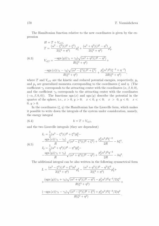
170 T. Vozmishcheva
The Hamiltonian function relative to the new coordinates is given by the ex-pression
(6.3)
H = T + Veff ,
T =(α2 − ξ2)(β2 + ξ2)
2(ξ2 + η2)p2
ξ +(α2 + η2)(β2 − η2)
2(ξ2 + η2)p2
η,
Veff =−sgn (y)(γ1 + γ2)
√(α2 + η2)(β2 − η2)
R(ξ2 + η2)+
−sgn (x)(γ1 − γ2)√
(α2 − ξ2)(β2 + ξ2)
R(ξ2 + η2)+
p2ϕα2β2(ξ−2 + η−2)
2R(ξ2 + η2),
where T and Veff are the kinetic and reduced potential energies, respectively, pξ
and pη are generalized momenta corresponding to the coordinates ξ and η. (Thecoefficient γ1 corresponds to the attracting center with the coordinates (α, β, 0, 0),and the coefficient γ2 corresponds to the attracting center with the coordinates(−α, β, 0, 0)). The functions sgn (x) and sgn (y) describe the potential in thequarter of the sphere, i.e., x > 0, y > 0; x < 0, y < 0; x > 0, y < 0; x <0, y > 0.
In the coordinates (ξ, η) the Hamiltonian has the Liouville form, which makesit possible to write down the integrals of the system under consideration, namely,the energy integral
(6.4) h = T + Veff ,
and the two Liouville integrals (they are dependent)
(6.5)
I1 =1
2(α2 − ξ2)(β2 + ξ2)p2
ξ−
−sgn (x)(γ1 − γ2)
R
√(α2 − ξ2)(β2 + ξ2) +
p2ϕα2β2ξ−2
2R− hξ2,
I2 =1
2(α2 + η2)(β2 − η2)p2
η−
−sgn (y)(γ1 + γ2)
R
√(α2 + η2)(β2 − η2) +
p2ϕα2β2η−2
2R− hη2.
The additional integral can be also written in the following symmetrical form
L =(α2 − ξ2)(β2 + ξ2)η2
2(ξ2 + η2)p2
ξ −(α2 + η2)(β2 − η2)ξ2
2(ξ2 + η2)p2
η+
+(sgn (y)(γ1 + γ2)
√(α2 + η2)(β2 − η2)− p2
ϕα2β2η−2/2)ξ2
R(ξ2 + η2)+
(−sgn (x)(γ1 − γ2)√
(α2 − ξ2)(β2 + ξ2) + p2ϕα2β2ξ−2/2)η2
R(ξ2 + η2).
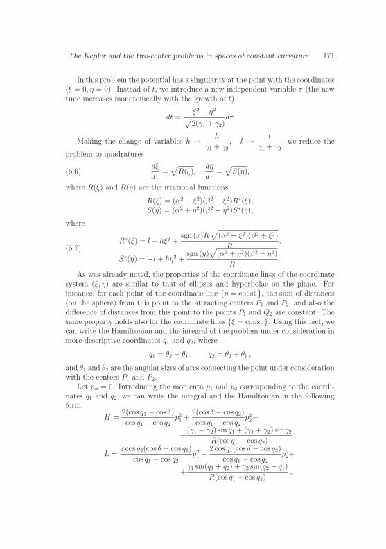
The Kepler and the two-center problems in spaces of constant curvature 171
In this problem the potential has a singularity at the point with the coordinates(ξ = 0, η = 0). Instead of t, we introduce a new independent variable τ (the newtime increases monotonically with the growth of t)
dt =ξ2 + η2
√2(γ1 + γ2)
dτ
Making the change of variables h → h
γ1 + γ2
, l → l
γ1 + γ2
, we reduce the
problem to quadratures
(6.6)dξ
dτ=
√R(ξ),
dη
dτ=
√S(η),
where R(ξ) and R(η) are the irrational functions
R(ξ) = (α2 − ξ2)(β2 + ξ2)R∗(ξ),S(η) = (α2 + η2)(β2 − η2)S∗(η),
where
(6.7)R∗(ξ) = l + hξ2 +
sgn (x)K√
(α2 − ξ2)(β2 + ξ2)
R,
S∗(η) = −l + hη2 +sgn (y)
√(α2 + η2)(β2 − η2)
R.
As was already noted, the properties of the coordinate lines of the coordinatesystem (ξ, η) are similar to that of ellipses and hyperbolae on the plane. Forinstance, for each point of the coordinate line η = const , the sum of distances(on the sphere) from this point to the attracting centers P1 and P2, and also thedifference of distances from this point to the points P1 and Q2 are constant. Thesame property holds also for the coordinate lines ξ = const . Using this fact, wecan write the Hamiltonian and the integral of the problem under consideration inmore descriptive coordinates q1 and q2, where
q1 = θ2 − θ1 , q2 = θ2 + θ1 ,
and θ1 and θ2 are the angular sizes of arcs connecting the point under considerationwith the centers P1 and P2.
Let pϕ = 0. Introducing the momenta p1 and p2 corresponding to the coordi-nates q1 and q2, we can write the integral and the Hamiltonian in the followingform:
H =2(cos q1 − cos δ)
cos q1 − cos q2
p21 +
2(cos δ − cos q2)
cos q1 − cos q2
p22−
−(γ1 − γ2) sin q1 + (γ1 + γ2) sin q2
R(cos q1 − cos q2),
L =2 cos q2(cos δ − cos q1)
cos q1 − cos q2
p21 −
2 cos q1(cos δ − cos q2)
cos q1 − cos q2
p22+
+γ1 sin(q1 + q2) + γ2 sin(q2 − q1)
R(cos q1 − cos q2),
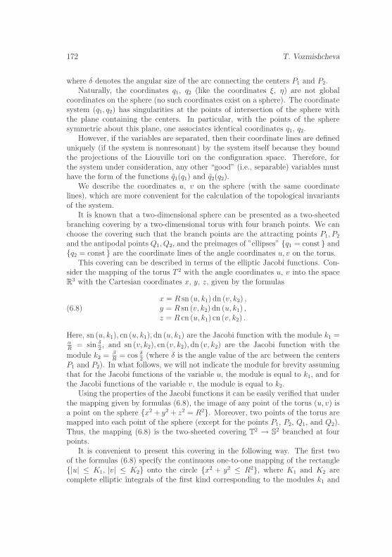
172 T. Vozmishcheva
where δ denotes the angular size of the arc connecting the centers P1 and P2.Naturally, the coordinates q1, q2 (like the coordinates ξ, η) are not global
coordinates on the sphere (no such coordinates exist on a sphere). The coordinatesystem (q1, q2) has singularities at the points of intersection of the sphere withthe plane containing the centers. In particular, with the points of the spheresymmetric about this plane, one associates identical coordinates q1, q2.
However, if the variables are separated, then their coordinate lines are defineduniquely (if the system is nonresonant) by the system itself because they boundthe projections of the Liouville tori on the configuration space. Therefore, forthe system under consideration, any other “good” (i.e., separable) variables musthave the form of the functions q1(q1) and q2(q2).
We describe the coordinates u, v on the sphere (with the same coordinatelines), which are more convenient for the calculation of the topological invariantsof the system.
It is known that a two-dimensional sphere can be presented as a two-sheetedbranching covering by a two-dimensional torus with four branch points. We canchoose the covering such that the branch points are the attracting points P1, P2
and the antipodal points Q1, Q2, and the preimages of ”ellipses” q1 = const andq2 = const are the coordinate lines of the angle coordinates u, v on the torus.
This covering can be described in terms of the elliptic Jacobi functions. Con-sider the mapping of the torus T 2 with the angle coordinates u, v into the spaceR3 with the Cartesian coordinates x, y, z, given by the formulas
(6.8)x = R sn (u, k1) dn (v, k2) ,y = R sn (v, k2) dn (u, k1) ,z = R cn (u, k1) cn (v, k2) .
Here, sn (u, k1), cn (u, k1), dn (u, k1) are the Jacobi function with the module k1 =αR
= sin δ2, and sn (v, k2), cn (v, k2), dn (v, k2) are the Jacobi function with the
module k2 = βR
= cos δ2
(where δ is the angle value of the arc between the centersP1 and P2). In what follows, we will not indicate the module for brevity assumingthat for the Jacobi functions of the variable u, the module is equal to k1, and forthe Jacobi functions of the variable v, the module is equal to k2.
Using the properties of the Jacobi functions it can be easily verified that underthe mapping given by formulas (6.8), the image of any point of the torus (u, v) isa point on the sphere x2 + y2 + z2 = R2. Moreover, two points of the torus aremapped into each point of the sphere (except for the points P1, P2, Q1, and Q2).Thus, the mapping (6.8) is the two-sheeted covering T2 → S2 branched at fourpoints.
It is convenient to present this covering in the following way. The first twoof the formulas (6.8) specify the continuous one-to-one mapping of the rectangle|u| ≤ K1, |v| ≤ K2 onto the circle x2 + y2 ≤ R2, where K1 and K2 arecomplete elliptic integrals of the first kind corresponding to the modules k1 and
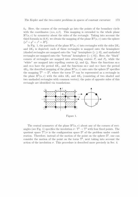
The Kepler and the two-center problems in spaces of constant curvature 173
k2. Here, the corners of the rectangle go into the points of the boundary circlewith the coordinates (±α,±β). This mapping is extended to the whole planeR2(u, v) by symmetry about the sides of the rectangle. Taking into account thethird formula in (6.8), we obtain the mapping of the plane R2(u, v) onto the spherex2 + y2 + z2 = R2.
In Fig. 1, the partition of the plane R2(u, v) into rectangles with the sides 2K1
and 2K2 is depicted; each of these rectangles is mapped onto the hemisphere(shaded rectangles are mapped onto the “top” hemisphere z ≥ 0, and unshadedrectangles are mapped onto the “bottom” hemisphere z ≤ 0). Here, the “black”corners of rectangles are mapped into attracting centers P1 and P2, while the“white” are mapped into repelling centers Q1 and Q2. Since the functions sn uand cn u have the period 4K1, and the functions sn v and cn v have the period4K2, the described mapping of the plane R2(u, v) onto onto the sphere S2 specifiesthe mapping T2 → S2, where the torus T2 can be represented as a rectangle inthe plane R2(u, v) with the sides 4K1 and 4K2 (consisting of two shaded andtwo unshaded rectangles with common vertex); the pairs of opposite sides of thisrectangle are identified via translations.
K2
K1u
v
Figure 1.
The central symmetry of the plane R2(u, v) about any of the corners of rect-angles (see Fig. 1) specifies the involution σ : T2 → T2 with four fixed points. Thequotient space T2/σ is the configuration space S2 of the problem under consid-eration. Therefore, instead of the motion of the point on the sphere S2, one canconsider the motion of the point on the torus T2, next taking into account theaction of the involution σ. This procedure is described more precisely in Sec. 4.
174 T. Vozmishcheva
The Hamiltonian and the additional integral in the variables u, v (i.e., describ-ing the motion of the point on the torus T2) have the form
H =p2
u + p2v
2(sin2 δcn 2u + cos2 δcn 2v
)−
−(γ1 − γ2) sin δsn udn u + (γ1 + γ2) cos δsn vdn v
R(sin2 δcn 2u + cos2 δcn 2v
) ,
L =cotan δcn 2vp2
u−tan δcn 2up2v
2(tan δcn 2u + cotan δcn 2v
)−
−(γ1−γ2) cos δsn udn ucn 2v−(γ1+γ2) sin δsn vdn vcn 2u
R(tan δcn 2u + cotan δcn 2v
) ,
where pu and pv are the momenta corresponding to the coordinates u, v.
7 Regularization
The potential V of the problem under consideration has singularities at four pointson the sphere (the attracting centers P1 and P2 and repelling centers Q1 and Q2).Moreover, at the points P1 and P2, the function V tends to −∞, and at thepoints Q1 and Q2 it tends to +∞. Since the kinetic energy T is always positiveand the total energy H = T + V is constant along the trajectories of the system,this implies that the particle moving on the sphere in the field generated by thepotential V never reaches the points Q1 and Q2. For the points P1 and P2, thesituation is just opposite: for any location of a particle on the sphere, we canset an initial velocity such that this particle reaches the attracting center for afinite time. Moreover, the velocity of the particle “at the instant of falling on theattracting center” becomes infinitely large (because T + V = const ).
Thus, the two-center problem on a sphere is described by the Hamiltoniansystem on the cotangent bundle to the two-dimensional sphere T ∗S2 with theHamiltonian H = T + V , where T is a function quadratic in momenta (thestandard metric on the sphere), and V is the function on the sphere given byformula (5.1). However, in this approach, the phase space of this system is notthe whole manifold T ∗S2, because the function V is not defined at four points P1,P2, Q1, and Q2 of the sphere (and, therefore, the function H is not defined onfour planes which are fibers of the cotangent bundle T ∗S2 over these four points).
Denote by S0 the sphere S2 with four points P1, P2, Q1, and Q2 removed.Then the phase space of the system is T ∗S0. As was already noted above, theHamiltonian vector field w = sgrad H on T ∗S0, which specifies the system, isnot complete. Therefore, although the system has the additional integral L (seeSec. 3), it is not Liouville integrable. Nevertheless, as will be shown below, aftera certain regularization the qualitative behavior of the system will be the sameas that of Liouville integrable Hamiltonian systems (almost all trajectories areconditionally periodic windings of tori).
The Kepler and the two-center problems in spaces of constant curvature 175
Note that the method for regularizing the system described below is similarto the regularization proposed by T. Levi-Civita for the classical Kepler problem.
Consider the Hamiltonian H as a function of the variables (u, v, pu, pv). Asystem with such a Hamiltonian can be considered as a Hamiltonian system onthe cotangent bundle to the torus T2. Introduce the notation
(7.1) λ(u, v) = sin2 δcn 2u + cos2 δcn 2v .
Then the Hamiltonian has the form
H =p2
u + p2v
2λ(u, v)− (γ1 − γ2) sin δsn udn u + (γ1 + γ2) cos δsn vdn v
R · λ(u, v),
and the coordinates of the field W = sgrad H on T ∗T2 are equal to(
∂H
∂pu
,∂H
∂pv
,−∂H
∂u,−∂H
∂v
).
In the phase space T ∗T2, the vector field W has singularities at the pointswhere λ(u, v) = 0, i.e., at the points (±K1,±K2, pu, pv). Consider the vector fieldW = λ(u, v) · sgrad H. In the coordinates (u, v, pu, pv) it has the form
(7.2)
(pu, pv, sin δcn u
(γ1 − γ2
R(2dn 2u− 1)− 2 sin δsn udn u · h
),
cos δcn v
(γ1 + γ2
R(2dn 2v − 1)− 2 cos δsn vdn v · h
)),
where h = H(u, v, pu, pv) is the value of the Hamiltonian at the point (u, v, pu, pv).The vector field W also has singularities at the points(±K1,±K2, pu, pv) because the Hamiltonian H is not defined at the points whereλ(u, v) = 0. Denote by Wh the restriction of the vector field W to the isoenergysurface Qh = H = h ⊂ T ∗T2. The vector field Wh already has no singularities(but it is defined only on the three-dimensional surface Qh). It is specified byformula (7.2) and, in particular, is defined at the points (±K1,±K2, pu, pv) lyingon the surface Qh, i.e.,
Wh(±K1,±K2, pu, pv) = (pu, pv, 0, 0) .
It is clear that integral trajectories of the field Wh coincide (with an accu-racy up to the change of a parameter) with integral trajectories of the initialvector field W = sgrad H on T ∗T2, since the multiplication of the field W by the
function λ(u, v) can be treated as the change of time:dt
dτ= λ(u(t), v(t)), where
(u(t), v(t), pu(t), pv(t)) is the trajectory of the field W .On the other hand, the vector field Wh on the surface Qh coincides with the
restriction to this surface of a certain vector field defined on the whole phase space
176 T. Vozmishcheva
T ∗T2. It is clear that such a continuation is not unique. For instance, as a suchfield, we can take the field sgrad Fh, where
(7.3)Fh = λ(H − h) =
p2u + p2
v
2− h
(sin2 δcn 2u + cos2 δcn 2v
)−−γ1 − γ2
Rsin δsn udn u− γ1 + γ2
Rcos δsn vdn v .
Then sgrad Fh = λsgrad H + (H − h)sgrad λ. Since Fh = 0 = H = h, thevector field sgrad Fh is tangent to the surface Qh and coincides with the field Wh
on it.The integral L of the initial system is, obviously, the integral of the Hamil-
tonian system with the Hamiltonian Fh on the surface Fh = 0. Therefore,after the described regularization the topological properties of the system withthe Hamiltonian H on T ∗T2 on each isoenergy surface Qh, will be similar to thoseof ordinary integrable Hamiltonian systems. In particular, nonsingular invari-ant manifolds of the system are Liouville tori and surgeries of these tori can bedescribed via the Fomenko–Ziecshang invariants.
Up to now, we, in fact, spoke about the regularization of the system on T ∗T2,which appeared from the consideration of the (branched) covering of the sphere S2
by the torus T2. This covering is defined by the involution σ : T2 → T2, describedin Sec. 3. The involution σ extends to an involution σ∗ : T ∗T2 → T ∗T2 in anatural way. Now, in order to return to the system on the sphere (and exactlythis system is the main subject of our study), it is necessary to take into accountthe action of the involution σ∗ on T ∗T2.
Since the involution σ : T2 → T2 is generated by the central symmetry ofthe plane R2(u, v) about the point (K1, K2) (or any other corner of rectangles inFig. 1), in the coordinates (u, v, pu, pv), the involution σ∗ has the form
(7.4) σ∗ : (u, v, pu, pv) → (2K1 − u, 2K2 − v,−pu,−pv) .
Therefore, the involution σ∗ has exactly 4 fixed points (±K1,±K2, 0, 0). Notethat the quotient space T ∗T2/σ∗ is not a manifold.
Now, we fix a certain value of h and consider the function Fh given by for-mula (7.3). It is easy to see that the surface Fh = 0 is invariant with respectto the involution σ∗ and does not contain the points (±K1,±K2, 0, 0) (a directcalculation shows that at these 4 points, the values of the function Fh are equal
to ±γi
Rsin δ, where i = 1, 2). Thus, the quotient spaces Fh = 0/σ∗ can be
considered as the isoenergy surfaces of the initial system on the sphere after theregularization.
Moreover, it is also easily verified that the vector field Wh on the surface Fh =0 is likewise invariant with respect to the involution σ∗, which makes it possibleto consider the vector field wh = Wh/σ
∗ as a result of the regularization of theinitial vector field w = sgrad H on the isoenergy surface Qh = H = h ⊂ T ∗S2.
The Kepler and the two-center problems in spaces of constant curvature 177
Thus, the above argument leads to the following statement describing the reg-ularization of the two-center problem on the sphere, i.e., the Hamiltonian systemw = sgrad H on the cotangent bundle to the sphere T ∗S2 with the HamiltonianH = T + V , where the function T quadratic in momenta is defined by the stan-dard metric on the sphere of radius R in R3, and the function V is given byformula (5.1).
Theorem 7.1 (on the regularization). Let h be a regular value of the Hamilto-nian H, and let Qh = H = h ⊂ T ∗S2 be the corresponding isoenergy surface.On the surface Qh, we consider the vector field wh = λsgrad H, where λ is func-tion (7.1) on the sphere S2.
Let f : T2 → S2 be the (branched) two-sheeted covering (6.8), letσ∗ : T ∗T2 → T ∗T2 be the corresponding involution (7.4), and let Fh be the func-tion defined by formula (7.3), on the cotangent bundle to the torus T ∗T2. On thesurface Fh = 0 ⊂ T ∗T2, consider the vector field Wh = sgrad Fh.
Then we have the following :
(1) the surface Fh = 0 ⊂ T ∗T2 is a closed three-dimensional manifold onwhich the involution σ∗ acts without fixed points ;
(2) on the surface Fh = 0, the vector field Wh has no singularities and isinvariant with respect to the involution σ∗;
(3) mapping (6.8) induces a diffeomorphism of the quotient space (with respectto the involution σ∗) of the surface Fh = 0 without points lying in 4fibers over the branch points of the mapping f onto the surface H = h ;moreover, this diffeomorphism transforms the vector field Wh into the vectorfield wh.
Note that the irregular values h of the Hamiltonian H are explicitly writtenin the construction of bifurcation diagrams.
178 T. Vozmishcheva
References
[1] T.G. Vozmischeva and A.A. Oshemkov, The topological analysis of the two-center problem on the two-dimensional sphere, Sbornik: mathematics, 2002,193(8), 3-38
[2] Ya.I. Granovsky, A.S. Zhedanov and I.M. Lutsenko, Quadratic algebras anddynamics in the curved space. I Oscillator, Theor. and Math. Physics, 1992,91, 2, 207–216.
[3] Ya.I. Granovsky, A.S. Zhedanov and I.M. Lutsenko, Quadratic algebras anddynamics in the curved space. II The Kepler problem, Theor. and Math.Physics, 1992, 91, 3, 396–410.
[4] V. V. Kozlov, On the dinamics in the spaces of constant curvature, Vestn.MGU, Ser. Mat. Mekh., 1994, No. 2, 28–35.
[5] P. W. Higgs, Dynamical symmetries in a spherical geometry. I, J. Phys. A:Math. Gen., 1979, 12, No 3, 309–323.
[6] N. A. Chernikov, The Kepler problem in the Lobachevsky space and its solu-tion, Acta Phys. Polonica, 1992, B23, 115–119.
[7] V. V. Kozlov and O. A. Harin, Kepler’s problem in constant curvature spaces,Cel. Mech. and Dyn. Astr., 1992, 54, 393–399.
[8] T. G. Vozmischeva, Classification of motions for generalization of the twocenter problem on a sphere, Cel. Mech. and Dyn. Astr., 2000, 77, 37–48.
[9] T. G. Vozmischeva, The Lagrange and Two-center Problems in theLobachevsky Space, Cel. Mech. and Dyn. Astr., 2002, 84, No 1, 65–85.
T.G. VozmishchevaIzhevsk State Technical UniversityApplied Mathematics Department Applied Mathematics and Computer Sci-ence ChairIzhevsk, Studencheskaya st. 7, [email protected], [email protected]
Travaux mathematiques, Volume 18 (2008), 179–200, c© Universite du Luxembourg
Sur la desintegration de larepresentation de conjugaison des
groupes de Lie nilpotents1
by Fatma Khlif
Resume
Nous presentons dans ce papier une desintegration en irreductibles dela representation de conjugaison d’un groupe de Lie nilpotent connexe etsimplement connexe. Nous construisons aussi un operateur d’entrelacementexplicite pour cette desintegration.
Classification Mathematique par Matieres. 22E27.
Mots-clef. Representation de conjugaison, operateur d’entrelacement, double-classe.
1 Introduction
Soit G un groupe localement compact de fonction module ∆G. On definit larepresentation de conjugaison (γG, L2(G)) de G par
γG(x)ξ(y) = ∆12G(x)ξ(x−1yx), ξ ∈ L2(G), x, y ∈ G.
Il est clair que γG est triviale sur le centre Z(G) de G. Soient (π,Hπ) et (π′,Hπ′)deux representations unitaires de G. On appelle operateur d’entrelacement entreπ et π′ tout operateur lineaire et borne U : Hπ → Hπ′ tel que U π(g) = π′(g)Upour tout g ∈ G. L’espace des operateurs d’entrelacement est note Hom(π, π′). Ondit que π et π′ sont equivalentes et on note π ' π′ s’il existe un operateur unitairedans Hom(π, π′). Soient maintenant S et T deux ensembles de representationsde G,. On dit que S est faiblement contenu dans T , qu’on note S ≺ T , si∩σ∈Sker(σ) ⊇ ∩τ∈T ker(τ). On dit aussi que S et T sont faiblement equivalents eton note S ∼ T , si S ≺ T et T ≺ S. Le support d’une representation ρ de G estdefini par
suppρ = π ∈ G, π ≺ ρ.1This work was supported by the CMCU contract 03/S 1502
180 F. Khlif
Alors il est clair que suppγG ⊂ G/Z(G), et que l’inclusion peut etre stricte(Voir [4], [6] et [7]). Cette egalite a ete etablie pour les groupes de Lie compacts etconnexes (voir [11]), les groupes de Lie simplement connexes nilpotents de classemaximale, les produits semi-directs de la forme Rn Rn (voir [9]).
Dans [6], E. Kaniuth a montre que
suppγG ∼ π ⊗ π, π ∈ Gpour les groupes σ-compacts et moyennables.
Dans ce papier, on se propose dans une premiere etape de montrer que siG est un groupe de Lie nilpotent connexe et simplement connexe, alors γG estequivalente a
∫ ⊕G
πl,−ldµ(πl), pour une certaine mesure dµ sur G et certainesrepresentations unitaires πl,−l speciales de G (voir 3.4). Ensuite, on ecrit unedesintegration en irreductibles de la representation γG en faisant intervenir desformules de desintegrations des representations induites [2] et des restrictions desrepresentations unitaires et irreductibles des groupes de Lie nilpotents [1]. Finale-ment, on construit un operateur d’entrelacement explicite pour cette desintegration.
2 Definitions et rappels
2.1 Mesures sur les sous-groupes de Lie nilpotents
Soit G un groupe de Lie connexe, simplement connexe et nilpotent d’algebre de Lieg. En notant exp l’application exponentielle, on ecrit G = exp g. Soit B = exp b
un sous-groupe connexe ferme de G.Nous appelons base de Jordan-Holder de b toute base Y = Y1, . . . , Yk de b
telle que le sous-espace bi := vecYi, ..., Yk soit un ideal de b pour i = 1, ..., k. Lasuite d’ideaux (bi)
k+1i=1 , telle que bk+1 = 0, s’appelle suite de Jordan-Holder de b
associee a Y .Une base de Malcev de g relative a b est par definition toute famille libre de
vecteurs X = X1, ..., Xn−k telle que vecXj, ..., Xn−k, b soit une sous-algebrede dimension n− j + 1 pour tout j = 1, ..., n− k. Alors les applications
Expb,Y : Rk → B, (t1, . . . , tk) 7→ exp t1Y1 · · · exp tkYk
et
Expgb : Rn−k → G/B, (t1, . . . , tn−k) 7→ exp t1X1 · · · exp tn−kXn−k ·B
sont des diffeomorphismes.L’espace de Schwartz S(G) de G est donne par l’ensemble des fonctions ϕ :
G → C verifiant ϕ Expg,Z ∈ S(Rn), ou Z est une base de Jordan-Holder de g etou S(Rn) designe l’espace de Schwartz ordinaire des fonctions C∞ a decroissancerapide sur l’espace vectoriel reel Rn.
Desintegration des representations de conjugaison 181
On choisit une mesure db sur B de la maniere suivante. Si η ∈ Cc(B), l’espacedes fonctions continues sur B a support compact, on pose
∫
B
η(b)db :=
∫
Rk
η(exp t1Y1 · · · exp tkYk)dt1 . . . dtk.
Cette mesure est invariante a gauche, donc une mesure de Haar. D’autre part siX = X1, . . . , Xn−k une base de Malcev de g relative a b, alors la mesure dX surG/B definie pour toute fonction continue a support compact η sur G/B par
∫
G/B
η(g)dX (g) :=
∫
Rn−k
η(Expgb(t))dt
est aussi G-invariante.
2.2 Representations induites
Soit G un groupe de Lie nilpotent connexe et simplement connexe d’algebre deLie g. Soit l une forme lineaire sur g et bl la forme bilineaire definie par bl(X, Y ) =〈l, [X, Y ]〉, X, Y ∈ g. On dit qu’une sous-algebre de Lie h de g est subordonnee a l sielle est totalement isotrope pour bl, c.a.d bl(h, h) = 0. On note S(l, g) l’ensemblede telles sous-algebres et M(l, g) celui des sous-algebres qui sont en meme tempsdes sous-espaces totalement isotropes pour bl et maximaux. Un element h deM(l, g) sera appele polarisation en l dans g, et par abus de language, le sous-groupe de Lie associe H = exp h sera aussi appele polarisation en l dans G. SoitZ une base de Jordan-Holder de g. On obtient une polarisation p(l) en l ∈ g∗
particuliere, appelee polarisation de Vergne relative a Z, de la facon suivante.Soit (gj)
n+1j=1 la suite de Jordan-Holder de g associee a Z. Alors
p(l) :=n∑
j=1
gj(l|gj).
Ici pour une algebre de Lie g et une forme lineaire l ∈ g∗, le symbole g(l) designele stabilisateur de l dans g, c. a d. g(l) = X ∈ g; 〈l, [X, g]〉 = 0.
Soit h ∈ S(l, g) et H = exp h. On definit le caractere χl de H par χl(exp X) =e−i〈l,X〉, X ∈ h. On construit la representation induite τl := τl,H := IndG
Hχl de Gde la facon suivante. Soit
S(G/H, χl) := ξ : G → C; ξ(gh) = χl(h−1)ξ(g), pour tout g ∈ G, h ∈ H,
ξ Expgh ∈ S(Rn−k),
pour une base (et alors pour toute base) de Malcev X = X1, . . . , Xn−k de g
relative a h. Nous munissons S(G/H, χl) de la norme
‖ξ‖22 :=
∫
G/H
|ξ(g)|2dX (g), ξ ∈ S(G/H, χl).
182 F. Khlif
Comme la mesure dX est G-invariante, la translation a gauche dans S(G/H, χl)est isometrique et definit la representation τl sur le complete L2(G/H,χl) deS(G/H, χl) pour la norme ‖.‖2.
D’apres la theorie de Kirillov, la representation τl,H est irreductible, si et seule-ment si H est une polarisation en l dans G. Dans ce cas-la, on ecrira πl au lieude τl. En outre, les representations πl,Bl
et πl,B′l sont equivalentes si et seulementsi Bl et B′
l sont deux polarisations en l dans G.
2.3 Representation conjuguee
Soit G un groupe localement compact et (π,Hπ) une representation de G. Onnote H′
π le dual C-lineaire de Hπ. D’apres le theoreme de Riesz, l’applicationHπ → H′
π, ξ 7→ fξ, definie pour tout η ∈ Hπ par fξ(η) = 〈ξ, η〉, est bijective etanti-lineaire. Munissons H′
π du produit scalaire 〈fξ, fη〉 = 〈ξ, η〉. La representationconjuguee π de G agit sur H′
π par π(g)fξ = fπ(g)ξ pour tout g ∈ G.
2.4 Integrale directe d’espaces de Hilbert
Soient G un groupe localement compact et X un espace localement compact, soit(πx,Hπx), x ∈ X un champ de representations unitaires de G et µ une mesuresur X. On note HX = ∪x∈XHπx et L2
0 = L20(X,HX , µ) l’ensemble des applications
f : X → HX telles que pour tout x ∈ X, f(x) ∈ Hπx et les fonctions x →‖f(x)‖Hπx
et (g, x) → 〈πx(g)[f(x)], f(x)〉 soient continues a support compact surX resp. sur G×X. On suppose que pour tout x ∈ X, le sous-espace f(x), f ∈ L2
0est dense dans Hπx . On munit L2
0 de la norme
‖f‖2 :=
√∫
X
‖f(x)‖2Hx
dµ(x).
On appelle alors integrale directe de (Hπx)x∈X , notee∫ ⊕
XHπxdµ(x), l’adherence
de L20 pour la norme ‖.‖2 et on definit la representation integrale directe π =∫ ⊕
Xπxdµ(x) de G agissant sur Hπ =
∫ ⊕XHπxdµ(x) par [π(g)f ](x) = πx(g)[f(x)]
pour tout g ∈ G, x ∈ X et f ∈ Hπ.
2.5 Espace de Garding
Soient G un groupe de Lie et du la mesure de Haar sur G, (π,Hπ) une representationunitaire de G, ξ ∈ Hπ et ϕ ∈ C∞
c (G), l’espace des fonctions infiniment differentiablesa support compact sur G. On appelle vecteur de Garding le vecteur π(ϕ)ξ definipar
π(ϕ)ξ =
∫
G
ϕ(u)π(u)ξ du.
Desintegration des representations de conjugaison 183
2.6 Operateurs de Hilbert-Schmidt
Soient H un espace de Hilbert, B(H) l’ensemble des operateurs bornes de H etA ∈ B(H). On dit que A est un operateur de Hilbert-Schmidt si l’operateur borneA∗A est tracable. L’ensemble des operateurs de Hilbert-Schmidt sera note HS(H),sur lequel on definit la norme suivante
‖A‖2HS = tr(A∗A).
En particulier pour une representation unitaire (π,Hπ) d’un groupe de Lie connexe,simplement connexe et nilpotent G = exp g et ϕ ∈ S(G), l’operateur π(ϕ) esttoujours de Hilbert-Schmidt. De plus, si π = πl ∈ G, l ∈ g∗ et ϕ ∈ S(G), alorsl’operateur πl(ϕ) est a noyau, c’est-a-dire on peut ecrire
πl(ϕ)ξ(x) =
∫
G/Bl
Kπl(ϕ)(x, g)ξ(g)dg, ξ ∈ Hπl, x ∈ G,
ou Bl est une polarisation en l dans G et Kπl(ϕ) est le noyau de πl(ϕ), qui estdonne par
Kπl(ϕ)(x, y) =
∫
Bl
ϕ(xby−1)χl(b)db, x, y ∈ G.
De plus Kπl(ϕ) ∈ S(G/Bl ×G/Bl, χl × χ−l) et l’application
S(G) → S(G/Bl ×G/Bl, χl × χ−l); ϕ 7→ Kπl(ϕ),
est continue et surjective (voir [5]).
2.7 Mesure de Plancherel
Soient G = exp g un groupe de Lie nilpotent connexe et simplement connexe,Z = Z1, . . . , Zn une base de Jordan-Holder de g et (gj)
n+1j=1 la suite de Jordan-
Holder de g associee a Z. On note pour tout j ∈ 1, . . . , n+1, dj(l) = dim(G·l|gj)
et dj = maxl∈g∗
dj(l). Soit E = l ∈ g∗, dj(l) = dj, j ∈ 1, . . . , n + 1 l’ouvert
G−invariant des orbites generiques. On considere les ensembles d’indices suivants
S = j ∈ 1, . . . , n; dj 6= dj+1, T = 1, . . . , n \ S.
Si on pose g∗S = vecZ∗j , j ∈ S et g∗T = vecZ∗
j , j ∈ T, on aura g∗ = g∗S⊕g∗T . Deplus, chaque G−orbite dans E rencontre g∗T en un seul point, en particulier E ∩g∗Test un ouvert de Zariski non vide dans g∗T . D’autre part, pour tout l ∈ E , la formebilineaire bl, definie par bl(X, Y ) = 〈l, [X, Y ]〉, X, Y ∈ g, est non degeneree. Ilexiste alors une fonction polynomiale, appelee le Pfaffien de l, qui verifie Pf(l)2 =det
(〈l, [Zi, Zj]〉)
i,j∈S. Soit K la bijection de Kirillov definie par
K : g∗/G 3 Ad∗G(l) 7→ [πl] ∈ G.
184 F. Khlif
Si dlT est la mesure euclidienne sur g∗T , alors l’application K : (E ∩ g∗T )/G → Genvoie la mesure dl = |Pf(l)|dlT en la mesure de Plancherel dµ sur G. Cette mesureintervient dans la desintegration de la representation reguliere gauche de G. Laformule de Plancherel dit que
‖ϕ‖22 =
∫
G
‖π(ϕ)‖2HSdµ(π) =
∫
E∩g∗T
‖πl(ϕ)‖2HS|Pf(l)|dlT , ϕ ∈ L2(G).
Par abus d’ecriture nous mettons aussi∫
g∗/G
dµ(πl) =
∫
G
dµ(π).
Nous definissons l’espace Hilbertien L2(G) comme integrale hilbertienne
L2(G) :=
∮
G
HS(Hπ)dµ(π).
2.8 Ensemble des double-classes
Soient H = exp h et B = exp b deux sous-groupes fermes connexes d’un groupede Lie G = exp g nilpotent, connexe et simplement connexe. On definit la double-classe relative a H et B d’un element g ∈ G, et on la note g = H · g · B, commeetant le sous-ensemble de G donne par H · g · B = h · g · b, (h, b) ∈ H × B.L’ensemble de toutes ces doubles-classes sera note HGB. Pour decrire cetensemble, on peut se referer au travail de Abdennadher et Ludwig [1]. Dans lasuite, on adopte leurs notations pour rappeler leur resultat. Soit Z = Z1, . . . , Znune base de Jordan-Holder de g. L’ideal engendre par Zi, . . . , Zn est note gi etGi son sous-groupe de Lie. On considere maintenant les sous-ensembles d’indicessuivants
Ig/h = i ∈ 1, . . . , n, Zi 6∈ h + gi+1, I = Ig/h ∩ Ig/b.
On note aussi I(h, b) le sous-ensemble de I caracterise par
i ∈ I(h, b) ⇐⇒
il existe un ouvert de Zariski non vide Ui ⊂ Gtel que pour tout g ∈ Ui, Zi 6∈ h + Adgb + gi+1.
On designe par Wi, i ∈ I, la partie de G donnee par
Wi =
g ∈ G, Zi 6∈ h + Adgb + gi+1 si i ∈ I(h, b)g ∈ G,Zi ∈ h + Adgb + gi+1 sinon.
Ces ensembles ont la propriete (P) de stabilite par la multiplication a droite avecles elements de B et a gauche avec les elements de H. De plus, chaque Wi contientun ouvert de Zariski maximal Ui non vide de G, ayant la propriete (P). On pose
U =⋂i∈IUi,
Desintegration des representations de conjugaison 185
qui est aussi un ouvert de Zariski de G verifiant (P). L’ensemble d’indices I(h, b),caracterisant l’ensemble des double-classes HGB, est alors
I(h, b) = i ∈ I, ∀g ∈ U , Zi 6∈ h + Adgb + gi+1.
On pose I(h, b) = i1 < · · · < id et on considere les applications suivantes
φ : Rd → G(t1, . . . , td) 7→ exp t1Zi1 · · · exp tdZid
etP : G → HGB
g 7→ g = H · g ·B.
Ainsi V = φ−1(U) est un ouvert de Zariski de Rd et U = P (U) est l’ensembledes double-classes de presque tous les elements de G. Avec cette constructionl’application
φ : V → U(t1, . . . , td) 7→ H · exp t1Zi1 · · · exp tdZid ·B
est un homeomorphisme. Dans la suite on notera Φ : U → G tel que Φ = φ φ−1.Dans le meme travail, Abdennadher et Ludwig [1] ont desintegre la mesure
invariante sur G/B en une integrale sur l’ensemble des double-classes. Si on prenddes bases de Malcev Y(g, h, b) et X de h relative a h ∩ Adgb respectivement deg relative a b qui varient rationnellement en g ∈ G, alors il existe une fonctionrationnelle F definie sur l’ensemble des double-classes telle que la mesure dγ,definie pour toute fonction ψ : HGB → C continue et a support compactdans U , par la relation∫
HGB
ψ(g)dγ(g) :=
∫
Vψ(H · exp t1Zi1 · · · exp tdZid ·B)|F (t1, . . . , td)|dt1 . . . dtd,
verifie(2.1)∫
G/B
ϕ(g)dX (g) =
∫
HGB
( ∫
H/H∩Φ(g)·B·Φ(g)−1
ϕ(h · Φ(g) ·B)dY(Φ(g),h,b)(h))dγ(g)
pour ϕ ∈ Cc(G/B).
2.9 Desintegration des restrictions de representations
Soient G un groupe de Lie nilpotent connexe et simplement connexe d’algebre deLie g, l ∈ g∗ et πl ∈ G. Soient Bl = exp bl une polarisation de G en l et H = exp h
un sous-groupe ferme connexe de G. La desintegration de πl|H sur l’ensemble desdouble-classes HGBl est donnee par Mackey dans [10] par
186 F. Khlif
πl|H '∫ ⊕
HGBl
IndHH∩Φ(g)·Bl·Φ(g)−1χ
Ad∗Φ(g)
(l)dγ(g)
avec une mesure γ sur HGBl. Un operateur d’entrelacement explicite pourcette desintegration est donne par Abdennadher et Ludwig dans [1] par
Srest : S(G/Bl, χl) −→∫ ⊕
HGBl
L2(H/H ∩ Φ(g) ·Bl · Φ(g)−1, χAd∗
Φ(g)(l))dγ(g)
tel que
(2.2) Srest(ξ)(g)(h) = ξ(h · Φ(g)),
ou ξ ∈ S(G/Bl, χl), g ∈ HGBl et h ∈ H.
2.10 Desintegration des representations induites
Soient G un groupe de Lie nilpotent connexe simplement connexe d’algebre deLie g, l ∈ g∗, H = exp h un sous-groupe de Lie ferme de G tel que 〈l, [h, h]〉 = 0et soit τl = IndG
Hχl la representation monomiale induite a partir du caractereunitaire χl. D’apres Corwin, Greenleaf [3] et Lipsman [8], la desintegration de τl
en irreductibles s’obtient comme suit
τl '∫ ⊕
(l+h⊥)/H
πfd(f),
d(f) etant une certaine mesure naturelle sur l’espace (l + h⊥)/H des H-orbites.Une desintegration concrete de τl est donnee par Baklouti et Ludwig [2], par laformule
(2.3) τl '∫ ⊕
VR,Bl
πfdλR,Bl (f),
ou VR,Bl est un sous-espace affine construit comme suit. Soit s = (gj)0≤j≤n une
suite d’ideaux de g verifiant
0 = gn+1 ⊂ gn ⊂ . . . ⊂ g1 = g
et Z = Z1, . . . , Zn la base de Jordan-Holder associee a s, c.a.d Zj ∈ gj/gj+1 etgj = Zj, . . . , Zn . On note hj = gj + h, j = 1, . . . , n et 1 ≤ j1 < . . . < jk ≤ n lesindices tels que hj 6= hj+1. Ainsi on construit a partir de Z une base de MalcevB = X1, . . . , Xk de g relative a h, dite extraite de la base Z, telle que Xi = Zji
.On pose alors
(2.4) VR,Bl = l +
r∑i=1
Ri(t)X∗i , t ∈ Rk ⊂ l + h⊥
Desintegration des representations de conjugaison 187
ou R = (R1, ..., Rr) est une famille de fonctions affines sur Rk, pour un certainr ∈ N, qui seront decrites en detail dans (4.1). De plus dλR,B
l est la mesure deLebesgue sur VR,B
l . Dans leur meme article, Baklouti et Ludwig ont construitun operateur d’entrelacement pour cette equivalence, en choisissant pour toutf ∈ VR,B
l et pour sa polarisation de Vergne relative a Z Bf = exp bf , certainesbases de Malcev Y(f) de bf relative a bf ∩ h, qui varient rationnellement avec f ,de sorte que l’operateur
(2.5) SInd : S(G/H,χl) −→∫ ⊕
VR,Bl
L2(G/Bf , χf )dλR,Bl (f)
defini pour tout ξ ∈ S(G/H, χl), f ∈ VR,Bl et g ∈ G par
SInd(ξ)(f)(g) =
∫
Bf /Bf∩H
ξ(gb)χf (b)dY(f)(b)
se prolonge sur L2(G/H, χl) en un operateur d’entrelacement unitaire pour l’equi-valence (2.3).
3 Desintegration de la representation de conju-
gaison
Il s’agit de donner dans cette partie une desintegration en irreductibles de larepresentation de conjugaison γG d’un groupe de Lie nilpotent connexe et simple-ment connexe G. Nous devons d’abord introduire certaines nouvelles representationsdu groupe G.
Definition 3.1. Soit l ∈ g∗ et Bl une polarisation en l. On definit la representation(πl,−l) de G dans l’espace hilbertien L2(G/Bl ×G/Bl, χl × χ−l) par
πl,−l(g)η(x, y) = η(g−1x, g−1y), x, y, g ∈ G.
Definition 3.2. Soit (π,Hπ) une representation unitaire et irreductible de G etA ∈ HS(Hπ), alors l’operateur π(g) A π(g−1) est aussi dans HS(Hπ) pourg ∈ G. On definit alors la representation (Cπ, HS(Hπ)) de G par
Cπ(g)A = π(g) A π(g−1), g ∈ G, A ∈ HS(Hπ).
En outre, la representation (C, L2(G)) de G est definie comme etant l’integralehilbertienne
C :=
∫ ⊕
G
Cπdµ(π).
Notre premier resultat s’enonce comme suit.
188 F. Khlif
Lemme 3.3. Soit l ∈ g∗ et Bl une polarisation de G en l. Alors pour πl = πl,Bl
on a queCπl
' πl,−l.
Demonstration. Notons HS0(Hπl) = πl(ξ), ξ ∈ S(G), qui est un sous-espace
dense de HS(Hπl). Nous savons d’apres [5], que l’application lineaire
U : HS0(Hπl) → L2(G/Bl ×G/Bl, χl × χ−l)
definie parU(πl(ξ)) := Kπl(ξ), ξ ∈ S(G),
envoie HS0(Hπl) sur l’espace S(G/Bl×G/Bl, χl×χ−l). Elle s’etend par continuite
en un operateur d’entrelacement unitaire entre Cπlet πl,−l. En effet, pour ξ ∈ Hπl
,on a
‖U(πl(ξ))‖2L2(G/Bl×G/Bl,χl×χ−l)
=
∫
G/Bl×G/Bl
|Kπl(ξ)(x, y)|2dxdy = ‖πl(ξ)‖2HS(Hπl
).
D’autre part, pour x, y ∈ G on a
U Cπl(g)(πl(ξ))(x, y) = KCπl
(g)(πl(ξ))(x, y) = Kπl(γG(g)(ξ))(x, y) = Kπl(ξ)(g−1x, g−1y)
= πl,−l(g)(Kπl(ξ))(x, y) = πl,−l(g) U(πl(ξ))(x, y).
¤
Theoreme 3.4. Soit G un groupe de Lie nilpotent connexe et simplement connexe.Soit µ la mesure de Plancherel de G. Alors
γG '∫ ⊕
g∗/G
πl,−ldµ(πl).
Demonstration. Il suffit de se rappeler que d’apres le theoreme de Plancherel,les espaces hilbertiens L2(G) et L2(G) =
∮G
HS(Hπ)dµ(π) sont isometriquementisomorphes et la transformation de Fourier
F (ξ)(π) := π(ξ), ξ ∈ L2(G) ∩ L1(G),
nous donne un tel operateur unitaire. En outre, F entrelace les representations γG
et C. En effet
F (γG(g)ξ)(π) = π(g)π(ξ)π(g−1) = Cπ(g)F (ξ)(π), ξ ∈ L2(G), g ∈ G.
Alors on a d’apres le lemme 3.3
γG '∫ ⊕
G
Cπdµ(π) '∫ ⊕
g∗/G
πl,−ldµ(πl).
¤
Desintegration des representations de conjugaison 189
L’etape suivante dans cette section consiste a ecrire une formule de desintegrationen irreductibles de la representation de conjugaison. Commencons par prouver laproposition suivante.
Proposition 3.5. On a :
γG '∫ ⊕
g∗/G
IndGBl
(χl|Bl⊗ π−l|Bl
)dµ(πl).
Demonstration. D’apres le theoreme 3.4, il suffit de montrer l’equivalence
πl,−l ' IndGBl
(χl|Bl⊗ π−l|Bl
),
ou l ∈ g∗ et Bl une polarisation de G en l. On note νl := IndGBl
(χl|Bl⊗ π−l|Bl
),donc νl est une representation de G qui agit sur l’espace hilbertien
Hνl:=
ψ : G → L2(G/Bl, χ−l), ψ mesurable,ψ(gb) = χl(b)
−1π−l(b)−1(ψ(g)), g ∈ G, b ∈ Bl,∫
G/Bl‖ψ(g)‖2
Hπ(−l)dX (g) < ∞
.
Nous verifions que si η ∈ L2(G/Bl × G/Bl, χl × χ−l), alors la fonction y 7→η(x, xy) =: V (η)(x)(y) est dans L2(G/Bl, χ−l) pour presque tout x ∈ G et que
V (η)(xb)(y) = η(xb, xby) = χl(b)−1π−l(b)
−1(V (η(x)))(y), y ∈ G, b ∈ Bl.
On peut donc considerer l’operateur
V : Hπl,−l−→ Hνl
defini parV (η)(x)(y) = η(x, xy), x, y ∈ G, η ∈ Hπl,−l
.
Il est clair que V est une isometrie. D’autre part, on verifie facilement que V πl,−l(g) = νl(g) V. En effet, pour x, y ∈ G, on a
(V πl,−l(g))η(x)(y) = πl,−l(g)η(x, xy) = η(g−1x, g−1xy)
= V (η)(g−1x, y) = (νl(g) V )η(x)(y).
Par consequent, les representations πl,−l et νl sont equivalentes. Le theoreme 3.4permet de conclure.
¤
En ce qui suit, on donne finalement la formule de la desintegration de γG enirreductibles.
190 F. Khlif
Theoreme 3.6. Soient g∗ 3 l 7→ Bl = exp bl un choix mesurable de polarisa-tions en l dans G et soit dγl, l ∈ g∗, la mesure sur l’ensemble des double-classesBlGBl =: GBl decrite dans 2.8. Pour g ∈ G, on note l(g) := l−Ad∗Φ(g)(l),
VR,Bl(g) le sous-espace affine de l(g) + (bl ∩ AdΦ(g)bl)
⊥ defini comme dans (2.4) et
dλR,Bl(g) la mesure de Lebesgue associee. On a alors
(3.1) γG '∫ ⊕
g∗/G
∫ ⊕
GBl
∫ ⊕
VR,Bl(g)
πl(g)+R(t)
dλR,Bl(g) (t)dγl(g)dµ(πl).
Demonstration. Pour tout l ∈ g∗ et Bl une polarisation en l dans G on a
IndGBl
(χl|Bl⊗ π−l|Bl
) ' IndGBl
(χl|Bl
⊗∫ ⊕
GBl
IndBl
Bl∩Φ(g)·Bl·Φ(g)−1χAd∗Φ(g)
(−l)dγl(g))
' IndGBl
∫ ⊕
GBl
IndBl
Bl∩Φ(g)·Bl·Φ(g)−1χl(g)dγl(g)
'∫ ⊕
GBl
IndGBl∩Φ(g)·Bl·Φ(g)−1χl(g)
dγl(g)
'∫ ⊕
GBl
∫ ⊕
VR,Bl(g)
πl(g)+R(t)
dλR,Bl(g) (t)dγl(g).
La proposition 3.5 nous permet de conclure. ¤
Corollaire 3.7. Soit G un groupe de Lie nilpotent connexe et simplement connexeet γG la representation de conjugaison associee, alors si L : G → g∗/G designel’application reciproque de la bijection de Kirillov, on a
L(suppγG) ⊂ (Ωπ − Ωπ)/G, π ∈ G,
ou Ωπ est l’orbite coadjointe de π.
Demonstration. Ce resultat decoule immediatement de la desintegration de larepresentation γG decrite dans le theoreme 3.6. En effet, pour tout l ∈ g∗ et g ∈ Gon a
l − Ad∗g(l) + (bl ∩ Adgbl)⊥ = l − Ad∗g(l) + (bl)
⊥ + (Adgbl)⊥
= (l + (bl)⊥)− (Ad∗g(l) + (Adgbl)
⊥) ⊂ Ωπl− Ωπl
.
¤
Desintegration des representations de conjugaison 191
4 Espace de desintegration
Dans cette partie, on ecrit une desintegration concrete de γG. Le lemme suivant estun outil indispensable dans la construction explicite de l’espace de desintegration.
Lemme 4.1. (voir [1]) On considere une famille F(t) = V 1(t), . . . , V k(t) dek vecteurs de Rn qui dependent polynomialement d’un parametre t ∈ Rn. Soitr = maxrang(F(t)), t ∈ Rn et soit e1, . . . , en la base canonique de Rn. On aalors le resultat suivant
1. Vr = t ∈ Rn, rang(F(t)) = r est un ouvert de Zariski de Rn.2. Pour tout i ∈ 1, . . . , n, l’ensemble t ∈ Rn, ei 6∈ vecF(t) ou bien son
complementaire, contient un ouvert de Zariski non vide de Rn.
Fixons une base de Jordan-Holder Z = Z1, . . . , Zn de g et adoptons lesnotations de 2.7. On a vu que chaque G−orbite dans E rencontre g∗T en un seulpoint, en particulier E ∩ g∗T est un ouvert de Zariski non vide dans g∗T . Soit q lecardinal de l’ensemble indice T = T1 < · · · < Tq. Identifions g∗T avec Rq a l’aidede l’application
w = (w1, . . . , wq) →q∑
j=1
wjZ∗Tj
=: lw.
Ainsi il existe un ouvert de Zariski O de Rq, tel que
γG '∫ ⊕
OIndG
Blw
((χlw)|Blw
⊗ (π−lw)|Blw
)|Pf(lw)|dw.
Dans la suite, on donnera une desintegration en irreductibles de (π−lw)|Blw
ense basant sur les resultats de Abdennadher et Ludwig [1]. Notons que l’existencedes differents ouverts de Zariski dans cette construction est due au lemme 4.1.On note Bw := Blw et bw := blw la polarisation de Vergne dans g en lw relativea la base de Jordan-Holder Z. Soit w ∈ O et i 6∈ Ig/bw , alors Zi ∈ bw + gi+1.Il existe Zi(w) = Zi +
∑nk=i+1 ai,k(w)Zk ∈ bw tels que ai,k(w)i+1≤k≤n soient les
solutions du systeme d’equations lineaires donne par 〈lw, [Zi(w), Zk]〉 = 0 pourtout k ∈ i, . . . , n. En reduisant si necessaire O on peut supposer que pour toutw dans l’ouvert de Zariski O on a
Ig/bw = j1, ..., jp.
D’autre part, d’apres le lemme 4.1, il existe un ouvert de Zariski W de Rq ×G etun ensemble d’indices i1, . . . , id ⊂ 1, . . . , n tel que pour tout w ∈ Rq verifiant(w ×G) ∩W 6= ∅,
I(bw, bw) = i ∈ Ig/bw ; Zi 6∈ bw + Adgbw + gi+1, ∀(w, g) ∈ W = i1, . . . , id.
192 F. Khlif
Notons aussi pour w ∈ Rq, tel que (w ×G) ∩W 6= ∅
φ = φw : Rd → G; φ(s) =d∏
k=1
exp skZik ,
Ww := g ∈ G; (w, g) ∈ W et Vw = φ−1w (Ww).
On obtient alors
πlw |Bw'
∫ ⊕
Vw
IndBw
Bw∩φ(s)·Bw·φ(s)−1χAd∗φ(s)
(lw)|Fw(s)|ds, s ∈ Vw
et d’apres l’egalite (2.1), Fw(s) est une fonction rationnelle en s et en w, doncelle est continue en (w, s) pour tout (w, φ(s)) dans l’ouvert de Zariski W et quidetermine la mesure sur l’ensemble des double-classes.
Passons maintenant a la construction d’un operateur d’entrelacement pourcette equivalence. On a vu que Zj1 , ..., Zjp est une base de Malcev de g relative abw, pour tout w ∈ O. De plus, si on note cIg/bw = 1, ..., n\Ig/bw = α1, ..., αn−p,alors on trouve une famille Zα1(w), ..., Zαn−p(w) de vecteurs de g qui forment unebase de Jordan-Holder de bw pour tous les w dans un ouvert de Zariski qu’on peutsupposer etre egal a O, en reduisant si necessaire O, et qui varient rationnellementet continument en w ∈ O.
On considere maintenant pour tout (w, s) tel que (w, φ(s)) ∈ W l’ensembled’indices
Ibw/bw∩Adφ(s)bw = αi, i ∈ 1, ..., n− p; Zαi(w) 6∈ bw ∩ Adφ(s)bw + (bw)i+1,
avec (bw)i+1 = vecZαi+1(w), ..., Zαn−p(w), i = 1, ..., n− p.
Comme precedement, en reduisant si necessaire W , on peut supposer qu’il existeune partie β1, ..., βe ⊂ α1, ..., αn−p telle que
Ibw/bw∩Adφ(s)bw = β1, ..., βe pour tout (w, φ(s)) ∈ W .
Ainsi Zβ1(w), ..., Zβe(w) est une base de Malcev de bw relative a bw ∩ Adφ(s)bw
pour tout (w, φ(s)) ∈ W . D’apres l’equation (2.2), l’operateur d’entrelacementpour la restriction est
Srest(w) : L2(G/Bw, χlw) →∫ ⊕
Vw⊂Rd
L2(Re, χAd∗φ(s)(lw))Fw(s)ds,
defini par
Srest(w)(ξ)(s1, . . . , sd)(z1, . . . , ze)
= ξ(exp z1Zβ1(w) · · · exp zeZβe(w) · exp s1Zi1 · · · sdZid).
Desintegration des representations de conjugaison 193
Il s’agit maintenant de desintegrer la representation
IndGBw∩φ(s)·Bw·φ(s)−1χlw+Ad∗φ(s)(−lw)
en se basant sur les resultats de Baklouti et Ludwig [2] dans le cadre de ladesintegration concrete des representations induites des groupes de Lie nilpotents.Soit (w, φ(s)) ∈ W , on note
lw(s) := lw + Ad∗φ(s)(−lw), b(w, s) := bw ∩ Adφ(s)bw.
Nous voyons que lw(s) varie polynomialement en (w, s). Il existe donc un ouvertde Zariski de Rq×G, qu’on peut supposer etre egal a W , et un ensemble d’indicesθ1, ..., θk ⊂ 1, ..., n, tel que Ig/b(w,s) = θ1, ..., θk pour tout (w, φ(s)) ∈ W .On note pour tout 1 ≤ j ≤ k , Xj = Zθj
. Ainsi B = X1, ..., Xk est une base deMalcev de g relative a toutes les sous-algebres de Lie b(w, s). Ecrivons
bi(w, s) := b(w, s) + vec Xi, ..., Xk et Bi(w, s) := exp bi(w, s), (w, φ(s)) ∈ W .
On note pour tout j ∈ 1, . . . , k, et (w, φ(s)) ∈ W , Γw,s := lw(s) + b(w, s)⊥
et dj(w, s) le maximum des dimensions des Bj(w, s)-orbites dans lw(s)|bj(w,s) +b(w, s)⊥ ⊂ [bj(w, s)]∗.Cette dimension maximale est donnee par le rang d’une matrice qui varie polyno-mialement en w et s. Soit
dj = max(w,φ(s))∈W
dj(w, s), d0 = 0 et L = j ∈ 1, ..., k; dj = dj−1 = λ1, ..., λr.
Alors, il existe un ouvert de Zariski, qu’on peut supposer etre egal a W , tel que
∀(w, φ(s)) ∈ W , dj(w, s) = dj, j = 1, ..., k.
Soit
(4.1) R = R1, . . . , Rk : Rr → Rk
la famille de fonctions affines definies sur Rr de la facon suivante. Soit t =(t1, ..., tr) ∈ Rr,
Rj(t) = ti, si j = λi ∈ L,
= 0, si j 6∈ L.
L’espace de desintegration de IndGB(w,s)χlw(s) est donne par
VR,Blw(s) = lw(s, t); t ∈ Rr ⊂ Γw,s
ou
lw(s, t) := lw(s) +k∑
j=1
Rj(t)X∗j .
194 F. Khlif
Ainsi pour tout (w, φ(s)) ∈ W , on trouve la desintegration suivante
(4.2) IndGB(w,s)χlw(s) '
∫ ⊕
Rr
πlw(s,t)dt,
avec πlw(s,t) = IndGB(w,s,t)χlw(s,t), B(w, s, t) = exp b(w, s, t) et b(w, s, t) est la pola-
risation de Vergne en lw(s, t) dans g relative a la base de Jordan-Holder Z.Pour la construction d’un operateur d’entrelacement pour cette equivalence,
on se propose tout d’abord de construire une base de Malcev de b(w, s, t) relativea b(w, s, t) ∩ b(w, s). On note comme avant, pour (w, φ(s), t) ∈ W × Rr
Ig/b(w,s,t) = i ∈ 1, ..., n, Zi 6∈ b(w, s, t) + gi+1.De nouveau, on peut supposer qu’il existe un ouvert de Zariski D de W × Rr etun ensemble indice m1, ..., mv ⊂ 1, ..., n tel que pour tout (w, φ(s), t) ∈ D onait
Ig/b(w,s,t) = κ1, ..., κv.On ordonne aussi l’ensemble indice
cIg/b(w,s,t) = 1, ..., n \ Ig/b(w,s,t) = ζ1, ..., ζn−v
Ainsi Zκ1 , ..., Zκv est une base de Malcev de g relative a b(w, s, t) pour tout(w, φ(s), t) ∈ D. D’autre part, pour (w, φ(s), t) ∈ D, on prend une base de Jordan-Holder de b(w, s, t)
Zζi(w, s, t) = Zζi
+n∑
j=ζi+1
a′i,j(w, s, t)Zj, i = 1, ..., n− v
qui varie rationnellement et meme, quitte a reduire D, continument sur D et onpose
(b(w, s, t))i = vecZζi(w, s, t), ..., Zζn−v(w, s, t), i = 1, ..., n− v,
et aussi
Ib(w,s,t)/b(w,s,t)∩b(w,s)
= ζi, i ∈ 1, ..., n− v; Zζi(w, s, t) 6∈ b(w, s, t) ∩ b(w, s) + (b(w, s, t))i+1.
On peut supposer de nouveau que pour tout (w, φ(s), t) ∈ D, on a
Ib(w,s,t)/b(w,s,t)∩b(w,s) = ϑ1, ..., ϑu.Ainsi Zϑ1(w, s, t), ..., Zϑu(w, s, t) est une base de Malcev de b(w, s, t) relative ab(w, s, t) ∩ b(w, s) pour tout (w, φ(s), t) ∈ D.
Desintegration des representations de conjugaison 195
Soit b = (b1, ..., bu) ∈ Ru, on note
Expb(w,s,t)b(w,s,t)∩b(w,s)(b) = exp(b1Zϑ1(w, s, t)) · · · exp(buZϑu(w, s, t)).
D’autre part, d’apres [2] et 2.10, il existe pour (w, s) fixe, un choix continu en tde bases de Malcev Y(w, s, t) de b(w, s, t) relative a b(w, s, t) ∩ b(w, s), tel quel’operateur
SInd(w, s) : S(G/B(w, s), χlw(s)) →∫ ⊕
Rr
Hπlw(s,t)dt,
SInd(w, s)ξ(t)(g) =
∫
B(w,s,t)/B(w,s,t)∩B(w,s)
ξ(gb)χlw(s,t)(b)dY(w,s,t)(b), g ∈ G,
realise une isometrie qui se prolonge en un operateur d’entrelacement unitaire pourl’equivalence (4.2). En fait les bases construites dans l’article [2] varient de faconrationnelle en t et il est facile de verifier que cette variation est aussi rationnelleen (w, s). Donc finalement les bases Y(w, s, t) sont continues en (w, s, t) pour tout(w, φ(s), t) dans un ouvert de Zariski, qu’on peut supposer etre egal a D.
Si on remplace la base Y(w, s, t) par une autre base Y ′(w, s, t), qui variecontinument en w, s et t, alors on obtient une fonction continue C(w, s, t) stricte-ment positive, telle que
dY(w,s,t) = C(w, s, t)dY ′(w,s,t),
Donc pour notre choix de la base Y ′(w, s, t) = Zϑ1(w, s, t), ..., Zϑu(w, s, t) ilexiste une fonction strictement positive continue C(w, s, t), pour laquelle l’operateurd’entrelacement
SInd(w, s) : S(G/B(w, s), χlw(s)
) −→∫ ⊕
Rr
L2(G/B(w, s, t), χlw(s,t)
)C(w, s, t)dt,
defini par
SInd(w, s)(ξ)(t)(g)
=
∫
Ru
ξ(g.Exp
b(w,s,t)b(w,s,t)∩b(w,s)(b)
)χlw(s,t)(Exp
b(w,s,t)b(w,s,t)∩b(w,s)(b))dY ′(w,s,t)(b), g ∈ G,
realise une isometrie qui se prolonge en operateur unitaire pour l’equivalence (4.2).
5 Operateur d’entrelacement
On rassemble maintenant les resultats des sections precedentes pour obtenir laforme finale de notre operateur d’entrelacement concret pour l’equivalence (3.1).
196 F. Khlif
Theoreme 5.1. Avec les notations plus haut, pour tout (w, φ(s), t) ∈ D, il existeune base de Malcev Y(w, s, t) de b(w, s, t) relative a b(w, s, t) ∩ b(w, s), pour la-quelle l’operateur defini par
S : S(G) −→∫ ⊕
Rq
∫ ⊕
Rd
∫ ⊕
Rr
L2(G/B(lw(s, t)), χlw(s,t))C(w, s, t)|Fw(s)| |Pf(lw)|dtdsdw,
tel que :
S(ξ)(w, s, t)(x)
=
∫
B(w,s,t)/B(w,s,t)∩B(w,s)
Kπlw (ξ)(xb, xbφ(s))χlw(s,t)(b)dY(w,s,t)(b)
=
∫
B(w,s,t)/B(w,s,t)∩B(w,s)
∫
Bw
ξ(xbb′φ(s)−1b−1x−1)χlw(b′)db′χlw(s,t)(b)dY(w,s,t)(b).
est une isometrie qui s’etend en un operateur unitaire qui entrelace γG et sadesintegration en irreductiles.
6 Exemples
Exemple 6.1. Soit g = vecX, Y1, ..., Yn, Z l’algebre de Lie filiforme de dimen-sion n + 2 tel que n ≥ 1 et de crochets non nuls
[X, Yi] = Yi+1, i ∈ 1, ..., n− 1, [X, Yn] = Z.
On peut identifier le groupe de Lie G = exp g avec le produit semi-direct expRXnexp a, avec a = vecY1, ..., Yn, Z. La representation de conjugaison γG est donnee,pour tout (x, a), (t, b) ∈ G et ξ ∈ L1(G), par
γG(t, b)ξ(x, a) = ξ((t, b)−1 · (x, a) · (t, b)) = ξ(b−1 · t−1 · x · a · t · b)= ξ(x · x−1 · b−1 · x · t−1 · a · t · b) = ξ(x, b− Adx−1b + Adt−1a).
Dans cet exemple on ecrit dans une premiere etape une desintegration en irreductiblesde la representation πl,−l, l ∈ g∗ et on donne l’operateur d’entrelacement associe.Ensuite, on en deduit une desintegration en irreductibles de γG. Soit l ∈ g∗ satis-faisant l(Z) 6= 0, on montre que
(6.1) πl,−l '∫ ⊕
Rπ(I−Ad∗exp sX)(l)ds =: ρl.

Desintegration des representations de conjugaison 197
SoitZ = X,Y1, ..., Yn, Z une base de Jordan-Holder de g et bl = vecY1, ..., Yn, Zla polarisation de Vergne relative a Z en tout l ∈ g∗ telle que l(Z) 6= 0 etBl = exp bl. On montre que l’operateur
S1 : S(G/Bl ×G/Bl, χl × χ−l) →∫ ⊕
RHπ(I−Ad∗
exp sX)(l)
ds
defini pour η ∈ S(G/Bl ×G/Bl, χl × χ−l) par
S1(η)(s)(exp uX) = η(exp uX, exp(u + s)X), u, s ∈ Rse prolonge par continuite surHπl,−l
en un operateur qui entrelace les representationsde l’equivalence (6.1). Dans la suite on note euX := exp uX et
δu(a) := exp uX · a · exp(−uX).
Soit l ∈ g∗ et g = ewX .a tels que w ∈ R et a = exp A ∈ exp a. On a
(S1 πl,−l(g))(η)(s)(euX) = πl,−l(g)(η)(euX , e(u+s)X) = η(g−1euX , g−1e(u+s)X)
= η(a−1e(u−w)X , a−1e(u−w+s)X)
= η(e(u−w)Xδw−u(a−1), e(u+s−w)Xδw−u−s(a
−1))
= χl(δ(w−u)(a))χ−l(δ(w−u−s)(a))η(e(u−w)X , e(u+s−w)X)
= e−i<l,Ade(w−u)X A>ei<l,Ad
e(w−u−s)X A>η(e(u−w)X , e(u+s−w)X)
= e−i<(I−Ad∗esX )(l),Ad
e(w−u)X A>η(e(u−w)X , e(u−w+s)X)
= χ(I−Ad∗
esX)(l)
(δ(w−u)(a))(S1(η))(s)(e(u−w)X)
= (S1(η))(s)(g−1euX) = π(I−Ad∗
esX)(l)
(g)(S1(η))(s)(euX)
= (ρl(g) S1)(η)(s)(euX).
D’autre part on a
‖S1(η)‖2Hρl
=
∫
R‖S1(η)(s)‖2
Hπ(I−Ad∗esX
)(l)ds =
∫
R
∫
R‖S1(η)(s)(euX)‖2duds
=
∫
R
∫
R‖η(euX , e(u+s)X)‖2duds = ‖η‖2
L2(G/Bl×G/Bl,χl×χ−l).
Par suite, d’apres (3.4), on a
γG '∫ ⊕
g∗/G
πl,−ldµ(πl) '∫ ⊕
Rn−1×R∗
∫ ⊕
Rπ(I−Ad∗
esX )l(y,z)|z|dsdy1 . . . dyn−1dz,
avec l(y,z) =n−1∑i=1
yiY∗i + zZ∗. Posons yn = 0, alors on a
Ad∗esX l(y,z) =n∑
j=1
( n∑i=j
(−s)i−j
(i− j)!yi +
(−s)n−j+1
(n− j + 1)!z)Y ∗
j + zZ∗.
198 F. Khlif
Par consequent
l(y,z)(s) := (I− Ad∗esX )l(y,z) =n−1∑j=1
( n∑i=j+1
−(−s)i−j
(i− j)!yi − (−s)n−j+1
(n− j + 1)!z)Y ∗
j .
Ainsi on trouve
γG '∫ ⊕
Rn−1×R∗
∫ ⊕
Rπl(y,z)(s)|z|ds dy dz.
L’operateur d’entrelacement est donne par
S : S(G) →∫ ⊕
Rn−1×R∗
∫ ⊕
RL2(R, χl(y,z)(s))|z|ds dy dz,
tel que
S(ξ)(y, z)(s)(x) = S1(Kπl(y,z)(s)(ξ))(s)(x) = Kπl(y,z)(s)
(ξ)(exX , e(x+s)X)
=
∫
Rn×Rξ(exXea1Y1 . . . eanYnetZe−(x+s)X)χl(y,z)(s)(e
a1Y1 . . . eanYnetZ) da1 . . . dan dt
=
∫
Rn×Rξ(e−sX ·
n∏
k=1
exp(k−1∑j=0
(x + s)j
j!ak−j
)Yk · exp
(t +
n∑j=1
(x + s)j
j!an−j+1)Z
)
e
−i
( n−1∑j=1
(n∑
i=j+1
−(−s)i−j
(i− j)!yi − (−s)n−j+1
(n− j + 1)!z)aj + tz
)
da1 . . . dandt.
Exemple 6.2. Soit g l’algebre de Lie de dimension 6 engendree par les vecteursA,B, C, U, V, Z et de crochets non nuls
[A,B] = Z, [B, C] = U et [C, A] = V.
D’apres le theoreme (3.4), on a
γG '∫ ⊕
(R×R∗)2π
l(a,u,v,z),−l(a,u,v,z)|u|da du dv dz
avec l(a,u,v,z) = aA∗+uU∗+vV ∗+zZ∗. La polarisation en l(a,u,v,z) dans g relative ala base de Jordan-Holder A,B, C, U, V, Z est b(a,u,v,z) = vecA+ v
uB,C, U, V, Z
qui est un ideal de g. Ainsi
γG '∫ ⊕
(R×R∗)2
∫ ⊕
RInd
G
B(a,u,v,z)χ
l(a,u,v,z)(s)|u|ds da du dv dz
avec l(a,u,v,z)(s) = (I− Ad∗exp sB)l(a,u,v,z) = −szA∗ + suC∗ et u, z ∈ R∗. Par suite
(6.2) γG '∫ ⊕
(R×R∗)2
( ∫ ⊕
R2
χ−szA∗+suC∗+t(B∗− vu A∗) |u|dt ds
)da du dv dz.
Desintegration des representations de conjugaison 199
D’apres (5.1), l’operateur d’entrelacement pour cette desintegration est donne,pour tout ξ ∈ S(G) et (a, u, v, z, s, t) ∈ R× R∗ × R× R∗ × R2, par
S(ξ)(a, u, v, z)(s, t) =
∫
RKπ(a,u,v,z)(ξ)(e
bB, e(b+s)B)e−itbdb.
Dans la suite on verifie avec un calcul explicite que S entrelace les representationsde l’equivalence (6.2).
‖S(ξ)‖22 =
∫
(R×R∗)2×R2
|∫
RKπ(a,u,v,z)(ξ)(e
bB, e(b+s)B)e−itbdb|2 |u|dt ds da du dv dz
=
∫
(R×R∗)2
∫
R2
|Kπ(a,u,v,z)(ξ)(etB, esB)|2 |u|dt ds da du dv dz
=
∫
(R×R∗)2‖Kπ(a,u,v,z)(ξ)‖2
L2(G/B(a,u,v,z)×G/B(a,u,v,z))|u| da du dv dz
=
∫
(R×R∗)2‖π(a,u,v,z)(ξ)‖2
HS(Hπ(a,u,v,z))|u| da du dv dz
= ‖ξ‖2L2(G).
D’autre part pour tout g = eβBh ∈ G tel que β ∈ R, h = eα(A+ vu
B)+λCmod Z(G),on note δβ(h) = eβBhe−βB. Alors on a
(S γG(g))(ξ)(a, u, v, z)(s, t) =
∫
RKπ(a,u,v,z)(γG(g)ξ)(e
bB, e(b+s)B)e−itbdb
=
∫
RKπ(a,u,v,z)(ξ)(g
−1ebB, g−1e(b+s)B)e−itbdb
=
∫
RKπ(a,u,v,z)(ξ)(h
−1e(b−β)B, h−1e(b−β+s)B)e−itbdb
=
∫
RKπ(a,u,v,z)(ξ)(e
bBδ−b(h−1), e(b+s)Bδ−(b+s)(h
−1))
· e−itbdb e−itβ
=
∫
RKπ(a,u,v,z)(ξ)(e
bB, e(b+s)B)χl(a,u,v,z)
(δ−b(h))
· χl(a,u,v,z)
(δ−(b+s)(h−1))e−itbdb e−itβ
=
∫
RKπ(a,u,v,z)(ξ)(e
bB, e(b+s)B)e−itbdb e−itβe−i(−sαz+suλ)
=
∫
RKπ(a,u,v,z)(ξ)(e
bB, e(b+s)B)e−itbdb
· χ−szA∗+suC∗+tB∗ (eβBeαA+λC)
200 F. Khlif
= S(ξ)(a, u, v, z)(s, t)χ−szA∗+suC∗+t(B∗− vu A∗)(g).
D’ou le resultat.
Remerciements. Je remercie vivement le Professeur J. Ludwig pour les discus-sions que j’ai eues avec lui a propos de ce sujet et la revision du manuscript. Jeremercie aussi le Referee pour les suggestions qu’il m’a faites pour la forme finalede cet article.
References
[1] J. Abdennadher et J. Ludwig, Ensemble des double-classes pour ladesintegration des representations des groupes de Lie nilpotents, preprint.
[2] A. Baklouti et J. Ludwig, Desintegration des representations monomiales desgroupes de Lie nilpotents, Journal of Lie theory, Volume 9(1999), 157–191.
[3] L. Corwin et F.P. Greenleaf, A canonical approach to multiplicity formulas forinduced and restricted representations of nilpotent Lie groups, Comm. Pureand Applied Math, XLI (1988), 1051–1088.
[4] E. Formanek, The conjugating representation and fusionless extensions, Proc.Amer. Math. Soc. 30(1971), 73–74.
[5] R. Howe, On a connection between nilpotent groups and oscillatory integralsassociated to singularities, Pac. J. Math. 73, 329–363 (1977).
[6] E. Kaniuth, On the conjugation representation of a locally compact group,Math. Z. 202(1989), 275–288.
[7] E. Kaniuth et A. Markfort Irreductible subrepresentations of the conjugationrepresentation of finite p-groups, J. Reine angew. Math.(2) 58(1953), 193–221.
[8] R. Lipsman, Orbital parameters for induced and restricted representation,Trans. Amer. Math. Soc. 313 (1989), 433–473.
[9] A. Markfort, On the support of the conjugation representation for solvablelocally compact groups, Forum Math. 6, No.4, 431–449 (1994).
[10] G.W. Mackey, The theory of unitary group representations, Chicago Lecturesin Mathematics. Chicago - London : The University of Chicago Press, (1976).
[11] M. Moskowitz, On a certain representation of a compact groups, J. Pure Appl.Algebras 36 (1985), 159–165.
Fatma KhlifDepartement de MathematiquesFaculte des Sciences de SfaxRoute de Soukra, 3038, Sfax, [email protected]
Table of Contents
Foreword . . . . . . . . . . . . . . . . . . . . . . . . . . . . . . . . . . . . . . . . . . . . . . . . . . . . . . . . . . . . . . . 5
List of Participants . . . . . . . . . . . . . . . . . . . . . . . . . . . . . . . . . . . . . . . . . . . . . . . . . . . 7–9
Conference papers
H. MaakestadJet bundles on projective space . . . . . . . . . . . . . . . . . . . . . . . . . . . . . . . . . . . . . 11–21
O.Petrenko, I.V.ProtasovAround Birkhoff Theorem . . . . . . . . . . . . . . . . . . . . . . . . . . . . . . . . . . . . . . . . . . 23–25
Y. AminovZero-emission surfaces of a moving electron . . . . . . . . . . . . . . . . . . . . . . . . . . 27–37
S. MaksymenkoHomotopy dimension of orbits of Morse functions on surfaces . . . . . . . . . 39–44
R. Jimenez, Y.V. MuranovOn surgery inside a manifold . . . . . . . . . . . . . . . . . . . . . . . . . . . . . . . . . . . . . . . . 45–64
P. Casati, G. OrtenziInonu–Wigner contraction to the truncated current Lie algebras . . . . . 65–75
A. Kowalik, I. Michalik, T. RybickiReconstruction theorems for two remarkable groups of diffeomorphisms 77–86
E. Krot-SieniawskaBernoulli-Taylor formula in the case of Q-umbral calculus . . . . . . . . . . . 87–92
I. YurchukOn the pseudoharmonic functions . . . . . . . . . . . . . . . . . . . . . . . . . . . . . . . . . 93–101
L. BazylevychHyperspaces of max-plus and max-min convex sets . . . . . . . . . . . . . . . 103–110
O. Shabat, M. ZarichnyiManifolds modeled on countable direct limits of absolute extensors 111–123
R. MatsyukSecond order variational problem and2-dimensional concircular geometry . . . . . . . . . . . . . . . . . . . . . . . . . . . . . . . 125–137
M. Nguiffo BoyomComplex of Nijenhuis and KV cohomology . . . . . . . . . . . . . . . . . . . . . . . . 139–160
Regular papers
T. VozmishchevaThe Kepler and the two-center problems in spaces of constantcurvature: on the regularization problem; Lie algebra of firstintegrals . . . . . . . . . . . . . . . . . . . . . . . . . . . . . . . . . . . . . . . . . . . . . . . . . . . . . . . . . 161–178
F. KhlifSur la desintegration de la representation de conjugaison desgroupes de Lie nilpotents . . . . . . . . . . . . . . . . . . . . . . . . . . . . . . . . . . . . . . . . . 179–200