typetheoretic approach to the shimming problem in ... · typetheoretic approach to the shimming...
TRANSCRIPT

Typetheoretic Approach to the Shimming
Problem in Scientific Workflows (Technical Report TR-BIGDATA-102013-KLC)
Andrey Kashlev, Shiyong Lu, Artem Chebotko
Wayne State University
Department of Computer Science
5057 Woodward Ave, Detroit, Michigan, 48202, USA
Abstract
When composing Web services into scientific workflows, users often face the so-called
shimming problem when connecting two related but incompatible components. The
problem is addressed by inserting a special kind of adaptors, called shims, that perform
appropriate data transformations to resolve data type inconsistencies. However,
existing shimming techniques provide limited automation and burden users with
having to define ontological mappings, generate data transformations, and even
manually write shimming code. In addition, these approaches insert many visible shims
that clutter workflow design and distract user’s attention from functional components
of the workflow. To address these issues, we 1) reduce the shimming problem to a
runtime coercion problem in the theory of type systems, 2) propose a scientific
workflow model and define the notion of well-typed workflows, 3) develop an
algorithm to typecheck workflows, 4) design a function that inserts “invisible shims”, or
runtime coercions into workflows, thereby solving the shimming problem for any well-
typed workflow, 5) implement our automated shimming technique, including all the
proposed algorithms, lambda calculus, type system, and translation function in our
VIEW system and present two case studies to validate our approach.
1 INTRODUCTION
Web Service composition plays a key role in the fields of services computing [1, 2, 3, 4, 5] and scientific workflows [6, 7, 8, 9]. Oftentimes composing autonomous third-party Web services into workflows requires using intermediate components, called shims, to mediate syntactic and semantic incompatibilities between different heterogeneous components.
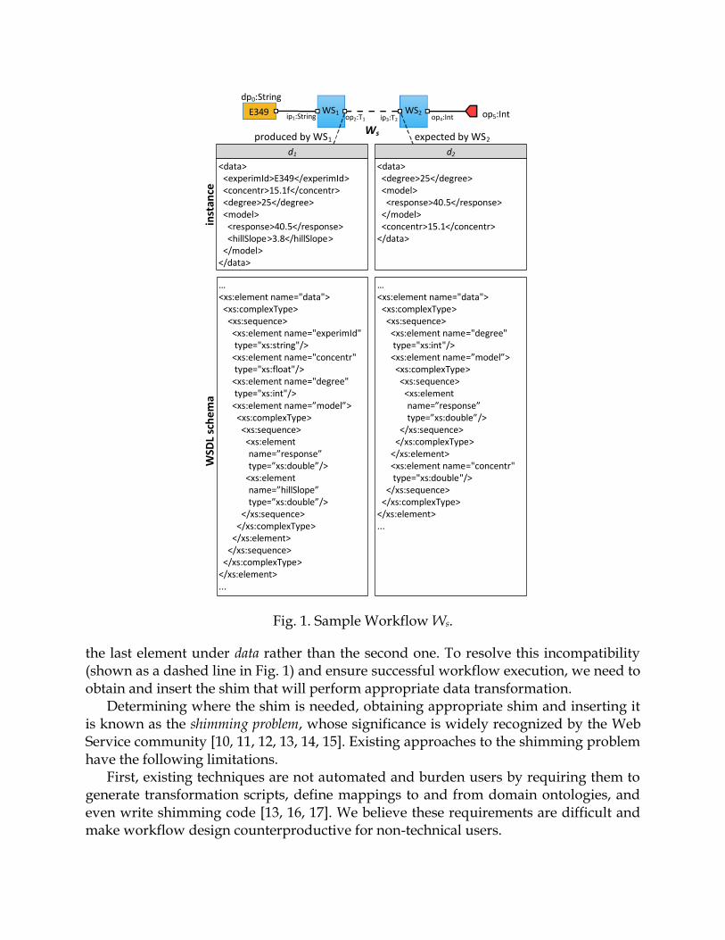
Consider a workflow Ws in Fig. 1 comprised of two Web services – WS1 and WS2. WS2 expects an XML document that differs from that returned by WS1. Particularly, WS2 expects an XML document with three child elements, rather than four, and the concentr element should be of type Double rather than Float. Besides, concentr element should be
dp0:String
op5:Intop4:Intop2:T1ip1:String ip3:T2
WS1 WS2
Ws
<data><experimId>E349</experimId><concentr>15.1f</concentr> <degree>25</degree> <model><response>40.5</response><hillSlope>3.8</hillSlope>
</model></data>
<data><degree>25</degree> <model>
<response>40.5</response></model><concentr>15.1</concentr>
</data>
…<xs:element name="data"><xs:complexType>
<xs:sequence><xs:element name="experimId" type="xs:string"/>
<xs:element name="concentr" type="xs:float"/>
<xs:element name="degree" type="xs:int"/>
<xs:element name=”model”><xs:complexType>
<xs:sequence><xs:element
______name=”response” ______type=”xs:double”/>
<xs:element ______name=”hillSlope” ______type=”xs:double”/>
</xs:sequence></xs:complexType>
</xs:element></xs:sequence>
</xs:complexType></xs:element>...
WSD
L sc
he
ma
inst
ance
…<xs:element name="data">
<xs:complexType><xs:sequence>
<xs:element name="degree" type="xs:int"/><xs:element name=”model”>
<xs:complexType><xs:sequence>
<xs:element ______name=”response” ______type=”xs:double”/>
</xs:sequence></xs:complexType>
</xs:element><xs:element name="concentr" type="xs:double"/>
</xs:sequence></xs:complexType>
</xs:element>...
d1 d2
E349
produced by WS1 expected by WS2
Fig. 1. Sample Workflow Ws.
the last element under data rather than the second one. To resolve this incompatibility (shown as a dashed line in Fig. 1) and ensure successful workflow execution, we need to obtain and insert the shim that will perform appropriate data transformation.
Determining where the shim is needed, obtaining appropriate shim and inserting it is known as the shimming problem, whose significance is widely recognized by the Web Service community [10, 11, 12, 13, 14, 15]. Existing approaches to the shimming problem have the following limitations.
First, existing techniques are not automated and burden users by requiring them to generate transformation scripts, define mappings to and from domain ontologies, and even write shimming code [13, 16, 17]. We believe these requirements are difficult and make workflow design counterproductive for non-technical users.

Second, current approaches produce cluttered workflows with many visible shims that distract users from main workflow components that perform useful work. Furthermore, recent workflow studies [18, 19] show that the percentage of shim components in workflows registered in myExperiment portal (www.myexperiment.org) has grown from 30% in 2009 [18] to 38% in 2012 [19]. These numbers indicate that such explicit shimming tends to make workflows even messier overtime, which further diminishes the usefulness of these techniques.
Third, many shimming techniques only apply under a particular set of circumstances that are hard to guarantee or even predict. Some approaches (e.g., [13, 16, 20, 21]) apply only when all the right shims are supplied by Web Service providers and are properly annotated beforehand, and/or when required shims can be generated by automated agents (e.g., XQuery–based shims [21]), which cannot be guaranteed for any practical class of workflows. Such uncertainty makes these techniques unreliable in the eyes of end users (domain scientists) who need assurance that their workflows will run.
Finally, while these efforts focus on resolving structural differences between complex types of Web services [13, 16, 20], they cannot mediate primitive types, such as Int or Double.
To address these issues, we propose a fully automated technique that, given a workflow creates and inserts suitable shims. Inserted shims transform data appropriately allowing successful workflow execution. Specifically, we
1. reduce the shimming problem to a runtime coercion problem in the theory of type systems,
2. propose a scientific workflow model and define the notion of well-typed workflows,
3. develop an algorithm to translate workflows into equivalent lambda expressions, 4. develop an algorithm to typecheck workflow expressions, 5. design a function that inserts “invisible shims” (coercions) into workflows,
thereby solving the shimming problem for any well-typed workflow, 6. implement our automated shimming technique and present two case studies to
validate the proposed approach to mediate Web services. To our best knowledge, this work is the first one to reduce the shimming problem to
the coercion problem and to propose a fully automated solution with no human involvement. Moreover, our technique frees workflow design from visible shims by dynamically inserting transparent coercions in workflows during execution time (implicit shimming). The proposed solution automatically mediates both structural data types, such as complex types of Web service inputs/outputs as well as primitive data types, such as Int and Double.
2 SCIENTIFIC WORKFLOW MODEL
Scientific workflows consist of one or more computational components connected to each other and possibly to some input data products. Each of these components can be viewed as a black box with well defined input and output ports. Every component is itself another workflow, either primitive or composite. Primitive workflows are bound to

executable components, such as Web services, scripts, or high performance computing (HPC) services and can be viewed as atomic entities. Composite workflows consist of multiple building blocks connected to one another via data channels. Each of these building blocks can be either a workflow or a data product. In the following we formalize the scientific workflow model used in this paper.
Definition 2.1 (Port). A port is a pair (id, type) consisting of a unique identifier and a data type associated with this port. We denote input and output ports as ipi:Ti and opj:Tj, respectively, where ipi and opj are identifiers, and Ti and Tj are port types.
Definition 2.2 (Data Product). A data product is a triple (id, value, type) consisting of a unique identifier, a value and a type associated with this data product. We denote each data product as dpi:Ti, where dpi is the identifier, and Ti is the type of the data product.
Given a workflow W, and the set of its constituent workflows W*, we use W.pj to denote port pj of W (be it input or output port) and W.W*.IP (W.W*.OP) to represent the union of sets of input (output) ports of all constituent workflows of W. Whenever it is clear from the context we omit the leading “W.”. Formally,
W*.IP = {ipi | ipi Wj.IP, Wj W*}
W*.OP = {opk | opk Wl.OP, Wl W*}
Definition 2.3 (Scientific workflow). A scientific workflow W is a 9-tuple (id, IP, OP, W*, DP, DCin, DCout, DCmid, DCidp), where
1. id is a unique identifier, 2. IP = {ip0, ip1, …, ipn} is an ordered set of input ports, 3. OP = {op0, op1,…, opm} is an ordered set of output ports,
4. W* = {W0, W1, …, Wp} is a set of constituent workflows used in W. Each Wi W* is another 9-tuple,
5. DP = {dp0, dp1, …, dpq} is a set of data products, 6. DCin : IP → W*.IP is an inverse-functional one-to-many mapping. DCin is a set of
ordered pairs:
DCin {(ipi, ipk) | ipi IP, ipk Wj.IP, Wj W*}
That is, each pair in DCin represents a data channel connecting input port ipi IP to
an input port ipk of some component Wj W*. 7. DCout : W*.OP → OP is an inverse-functional one-to-many mapping. DCout is a set
of ordered pairs:
DCout {(opj, opk) | opj Wi.OP, Wi W*, opk OP}. That is, each pair in DCout
represents a data channel connecting output port opj of some component Wi W* to an
output port opk OP. 8. DCmid : W*.OP → W*.IP is an inverse-functional one-to-many mapping. DCmid is a
set of ordered pairs:
DCmid {(opj, ipk) | opj Wl.OP, ipk Wm.IP, Wl, Wm W*}. That is, each pair in DCmid
represents a data channel connecting an output port opj of some component Wl W*
with an input port ipk of another component Wm W*. 9. DCidp : DP → W*.IP is an inverse-functional one-to-many mapping. DCidp is a set of

Fig. 2. Examples of scientific workflows (Wa, Wb, …, Wg).
ordered pairs:
DCidp {(dpi, ipk) | dpi DP, ipk Wj .IP, Wj W*}.
That is, each pair in DCidp represents a data channel that connects a data product dpi
DP to the input port ipk of some component Wj W*. Fig. 2 shows seven workflows that we will reference in this paper as Wa, Wb, Wc, Wd, We, Wf, and Wg respectively. These seven workflows use other workflows as their building blocks. Such constituent workflows are shown as blue boxes with their ids written inside each box. Ports appear as red pins pointing right (input) or left (output). Finally, data products are visualized as yellow boxes with their values placed inside (e.g., “true” in Wa in Fig. 2).
Because the order of input arguments of a workflow matters (e.g., Divide workflow in Wf in Fig. 2), we use ordered set IP to store a list of input ports. We use the term data channel to refer to a wire, connecting a workflow port to a data product or another port.
All enties from the set {DCin DCmid DCout DCidp} are data channels. As we show in later sections, a workflow is represented as a lambda expression. To
simplify lambda expressions, we focus on workflows with a single output port. We are currently extending our approach to allow set OP with a cardinality greater than one. Our definition requires that every workflow and every data product has a unique id. For simplicity we also require that for any workflow W, all ports of W and all ports of all workflows in W* have unique ids.
We model workflow Wd in Fig. 2 as a 9-tuple, where id = ”Wd”, IP = Ø, OP ={(op9, Float)}, W* = {Mean, Sqrt}, DP = {(dp0, 3, Int), (dp1, 5, Int), (dp2, 4, Int)}, DCin = Ø, DCout = {((Sqrt, op8), op9)}, DCmid = {((Mean, op6), (Sqrt, ip7))}, DCidp = {(dp0, (Mean, ip3)), (dp1, (Mean, ip4)), (dp2, (Mean, ip5))}. Workflow We, on the other hand does not have concrete input data products connected to its inputs. We model it using 9-tuple with id = ”We”, IP = {(ip0, Int), (ip1, Int), (ip2, Int)}, OP = {(op9, Double)}, W* = {Mean, Sqrt}, DP = Ø, DCin = {(ip0, (Mean, ip3)), (ip1, (Mean, ip4)), (ip2, (Mean, ip5))}, DCout = {((Sqrt, op8), op9)}, DCmid = {((Mean, op6), (Sqrt, ip7))}, DCidp = Ø.
Definition 2.4 (Primitive workflow). A workflow W is primitive if and only if it has both input ports and output ports, and W has neither constituent components, nor data
ip0:Int
ip1:Int
ip2:Int
ip3:Int
ip4:Int
ip5:IntMean Sqrt
op6:Float
ip7:Double op8:Double
We
op9:Double
IP DCin
OPDCmid DCout
Mean Sqrtop6:Float
ip7:Floatip3:Int
ip4:Int
ip5:Int
3
Wd
DCidpDP
DCmiddp0:Int
dp1:Int
dp2:Int
Increment
Square
Decrement
ip7:Int
ip8:Int
ip1:Int
op4:Intip3:Int
ip5:Int
op2:Int
op6:Int
dp0:Int
Divide
Wf Wg
Notip1:Bool
op2:Bool
ip3:Int
op4:Int
dp0:Booltrue Increment
Wa
Wbip1:Bool
op2:Int
dp0:Bool
true
ip0:BoolNot op2:Bool
ip3:IntIncrement
Wb
ip1:Bool
op4:Int
op5:Int
Wc
5
4
4
op5:Int
op9:Float
op8:Float
op10:Float
op9:Float
op3:Int
ip0:Int
op10:Float
op9:Floatip7:Int
ip8:Int
op4:Intip3:Int
ip5:Int
op2:Intip1:Int
op6:Int
Square
Increment
Decrement
Divide

products, nor data channels. Formally, W is primitive iff
W.IP ≠ Ø W.OP ≠ Ø W.W* = W.DP = W.DCin = W.DCout = W.DCmid = W.DCidp = Ø. We use isPrimitiveWF(W) to denote the above predicate.
Intuitively, primitive workflow is a black box that has inputs and outputs and that represents an atomic component, such as Web service. Primitive workflows are used by other workflows as building blocks. Workflows such as WS1, WS2, Not, Increment, Decrement, Sqrt, Square, Mean, and Divide in Fig. 1 and Fig. 2 are primitive workflows.
Definition 2.5 (Composite workflow). A workflow W is composite if and only if it contains at least one reusable component (i.e. W.W* ≠ Ø) connected to ports and/or data products. Formally, W is composite iff
(W.W* ≠ Ø W.IP ≠ Ø W.OP ≠ Ø W.DCin ≠ Ø W.DCout ≠ Ø) (W.W* ≠ Ø
W.OP ≠ Ø W.DP ≠ Ø W.DCidp ≠ Ø W.DCout ≠ Ø) We use isComposite(W) to denote the above predicate. All workflows Ws, Wa, Wb, …,
Wg in Fig. 1 and Fig. 2 are composite. Intuitively, reusable workflows are primitive or composite tasks that can be reused
as building blocks of more complex workflows. They are not executable as at least some of their input ports are not bound. Workflows Wb, We and Wg in Fig 2 are reusable. Workflow Wb is reused inside Wc. Executable workflows, on the other hand have all input data needed to perform computation. Workflows Ws, Wa, Wc, Wd, and Wf in Fig. 1 and Fig. 2 are executable. Each executable workflow must contain at least one component and one data product connected to it. Thus, every executable workflow is composite. The opposite is not true, as composite workflow may be reusable (e.g., Wb), i.e. have input port(s) instead of concrete data product(s).
3 WORKFLOW EXPRESSIONS
We rely on simply typed lambda calculus [22] enriched with a set of primitive types as a formal framework to reason about the behavior of workflows. For example, expression “λx:Int. Increment x” is a function, or abstraction, that takes one integer argument, and returns its value increased by 1. x is the abstraction name and “Increment x” is the expression of this abstraction. The expression “Increment 3” is an application, which evaluates to 4. Definition 3.1 (Workflow expression). Given a workflow W, its expression expr is a lambda expression that represents computation performed by W. If W is reusable, expr is an abstraction. If W is executable, expr is an application.
In this paper, we present our translateWorkflow function outlined in Algorithm 1, that given a workflow W, translates it into an equivalent lambda expression which performs the same computations and produces the same result as W. For simplicity we assume that workflow diagrams are drawn horizontally with data flowing from left to right (see Fig. 1, 2). Given a workflow W, our translateWorkflow algorithm translates all components in W into lambda functions, and builds an expression whose structure corresponds to composition of components in W. Each connection between two components becomes an application in the equivalent lambda expression.

Algorithm 1. Translating workflows into lambda expressions
1: function translateWorkflow 2: input: workflow W
3: output: lambda expression for W
4: if isPrimitiveWF(W) /* If W is primit., return its id */ then return W.id
5: else
6: /* Otherwise, W is composite (reusable or executable), translate it recursively into
__lambda expression: */
7: /* First, find component in W.W* that performs the very last computational step
__(componentProducingFinalRes): */
8: let outputPortsOfDCmid be an empty set
9: for each ((wj, opj), (wk, ipl)) W.DCmid do
10: add opj to outputPortsOfDCmid
11: end for
12: for each W' W.W* do
13: if W'.OP OutputPortsOfDCmid
14: then componentProducingFinalRes = W'
15: end if
16: end for
17: /* Build the list of expressions that serve as arguments for
___componentProducingFinalRes:*/
18: listOfArguments = “”
19: for each (idi, typei) componentProducingFinalRes.IP do
20: listOfArguments += getInputExpression(W, componentProducingFinalRes, idi)
___+ “ “
21: end for
22: if W is reusable //|W.DCin | > 0
23: /* translate it into lambda abstraction: */
24: then
25: listOfNames = “”
26: for each (idi, typei) W.IP do
27: listOfNames += “λx” + idi + “:” + typei + “. ”
28: end for
29: return “(” + listOfNames + translateWorkflow(componentProducingFinalRes)
___“ ” + listOfArguments + “)”
30: else
31: /* W is executable, thus translate it into a lambda application: */
32: return translateWorkflow(componentProducingFinalRes) + “ ” +
___listOfArguments;
33: end if
34: end if
35: end function

We accommodate composite workflows (containing sub-workflows) nested inside each other to arbitrary degree via recursive calls to translateWorkflow function that translates all sub-workflows at each level of nesting (depth-wise translation). We also accommodate arbitrary workflow compositions within the same level of nesting (flat compositions) by recursively calling getInputExpression function outlined in Algorithm 2, that iterates over and translates all the connected components by backtracking along the data channels from right to left (breadth-wise translation). Thus, our two algorithms together cover the full range of possible workflow compositions. We now provide a We accommodate composite workflows (containing sub-workflows) nested inside each other to arbitrary degree via recursive calls to translateWorkflow function that translates all sub-workflows at each level of nesting (depth-wise translation). We also accommodate arbitrary workflow compositions within the same level of nesting (flat compositions) by recursively calling getInputExpression function outlined in Algorithm 2, that iterates over and translates all the connected components by backtracking along the data channels from right to left (breadth-wise translation). Thus, our two algorithms
Algorithm 2. Algorithm for obtaining lambda expressions representing inputs at certain workflow ports
1: function getInputExpression 2: input: workflow W, constituent component c, input port ipm
3: output: lambda expression that serves as input argument of port W.id. 4: /* first, if there is a data product dpi in W.DP connected to port ipm, return dpi.id of that
data product: */ 5: for each (dpi, (wj, ipk)) W.DCidp do 6: if wj.id = c.id and ipk.id = ipm.id then return dpi.id end if 7: end for 8: /* if there is an input port ipj in W.IP connected to port ipm, return variable named “x” +
ipj.id */ 9: for each (ipj, (wk, ipl)) W.DCin do 10: if wk.id = c.id and ipl.id = ipm.id then return “x” + ipj.id end if 11: end for 12: /* if there is another constituent workflow wi whose output is connected to ipm, construct
the list of input arguments (expressions) of wi and return application of these arguments to
wi : */ 13: listOfArguments = “” 14: for each ((wi, opj), (wk, ipl)) W.DCmid do 15: if wk.id = c.id and ipl.id = ipm.id then 16: for ipq wi.IP do 17: listOfArguments += getInputExpression(W, wi, ipq) + “ ” 18: end for 19: return “(” + translateWorkflow(wi) + “ ” + listOfArguments + “)” 20: end if 21: end for 22: return “error - cannot obtain input expression” 23: end function

together cover the full range of possible workflow compositions. We now provide a walk-through example of how a workflow Wd is translated into an equivalent lambda expression.
Example 3.2 (Translating workflow Wd into an equivalent lambda expression). Consider a workflow Wd in Fig. 2. When the function translateWorkflow(Wd) is called, it first checks whether Wd is primitive, and because it is not, the else clause is executed (lines 5-34). translateWorkflow first determines that the component producing final result of the entire workflow Wd is Sqrt and stores it in the componentProducingFinalRes variable (line 14). Next, because Sqrt has a single input, for loop in lines 19-21 executes once, calling the function getInputExpression(Wd, Sqrt, ip7), whose output “(Mean dp0 dp1 dp2)” is stored into a string listOfArguments. Next, translateWorkflow checks whether Wd is reusable (line 22), and because it is not it returns the application of workflow expression for Sqrt component to the list of arguments obtained earlier (line 32). Since Sqrt is a primitive workflow, translateWorkflow(Sqrt) returns its name “Sqrt”. Thus, the final result of the translation is “Sqrt (Mean dp0 dp1 dp2)”.
Example 3.3 (lambda expressions for workflows Ws, Wa, Wb, …, Wg). We provide lambda expressions obtained by calling our translateWorkflow algorithm on each workflow in Fig. 1, 2:
Ws : WS2 (WS1 dp0) Wa : Increment (Not dp0) Wb : λx0:Bool. Increment (Not x0) Wc : Wb dp0 = (λx0:Bool. Increment (Not x0)) dp0 Wd : Sqrt (Mean dp0 dp1 dp2) We : λx0:Int. λx1:Int. λx2:Int. (Sqrt (Mean x0 x1 x2)) Wf : Divide (Increment (Square dp0)) (Decrement (Square dp0)) Wg : λx0:Int. Divide (Increment (Square x0)) (Decrement (Square x0))
Note that executable workflows (Ws, Wa, Wc, Wd, Wf) are translated into lambda applications, whereas reusable ones (Wb, We, Wg) into lambda abstractions. Ports are translated into variables, e.g. port ip0 appears as x0 in the corresponding expression. We require that the workflow expression is flat, i.e. constituent components’ ids are replaced with their translations (see expression for Wc). Thus, a workflow expression only contains port variables, names of primitive workflows, and data products.
4 TYPE SYSTEM FOR SCIENTIFIC WORKFLOWS
For interoperability, we adopt the type system defined in the XML Schema language specification [23]. This allows us to mediate WSDL-based Web services since their input and output types are described in WSDL documents according to the XSD format. While our approach can accommodate all types defined in [23], in this paper we focus on the set of types that are most relevant to the scientific workflow domain.
T ::= TPRIM | TXSD | T → T
TPRIM ::= String | Decimal | Integer | NonPositiveInteger | NegativeInteger |
NonNegativeInteger | UnsignedLong | UnsignedInt | UnsignedShort | UnsignedByte |
Double | PositiveInteger | Float | Long | Int | Short | Byte | Bool
TXSD ::= { e : TPRIM } | { e : TXSDi i = 1 … n
}
In our approach we allow primitive types (TPRIM), XSD types (TXSD), and arrow types (T
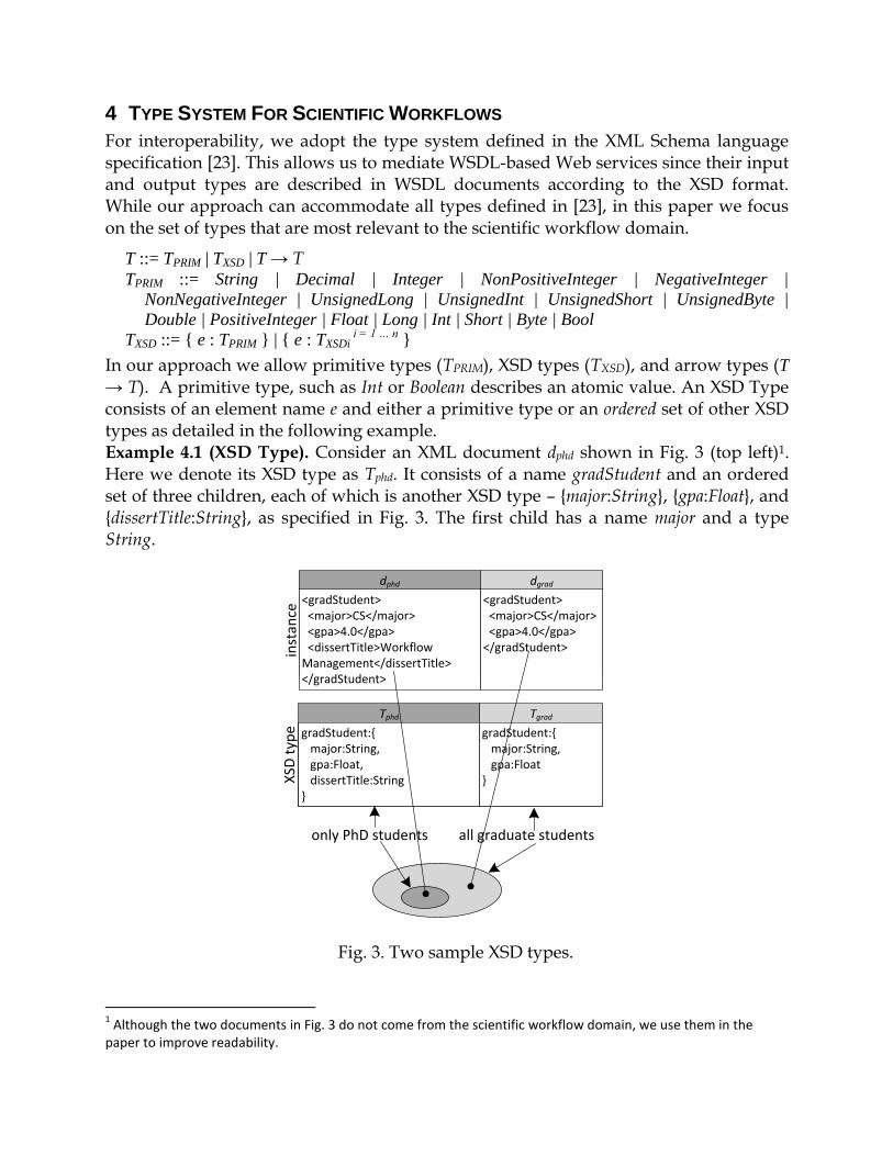
→ T). A primitive type, such as Int or Boolean describes an atomic value. An XSD Type consists of an element name e and either a primitive type or an ordered set of other XSD types as detailed in the following example. Example 4.1 (XSD Type). Consider an XML document dphd shown in Fig. 3 (top left)1. Here we denote its XSD type as Tphd. It consists of a name gradStudent and an ordered set of three children, each of which is another XSD type – {major:String}, {gpa:Float}, and {dissertTitle:String}, as specified in Fig. 3. The first child has a name major and a type String.
Fig. 3. Two sample XSD types.
1 Although the two documents in Fig. 3 do not come from the scientific workflow domain, we use them in the
paper to improve readability.
Tphd Tgrad
dphd dgrad
<gradStudent> <major>CS</major> <gpa>4.0</gpa> <dissertTitle>Workflow Management</dissertTitle></gradStudent>
gradStudent:{ major:String, gpa:Float, dissertTitle:String}
<gradStudent> <major>CS</major> <gpa>4.0</gpa></gradStudent>
gradStudent:{ major:String, gpa:Float}
inst
ance
XSD
typ
e
only PhD students all graduate students

In this work we adhere to such notation for describing XSD types due to its conciseness compared to traditional XML Schema syntax. To improve readability, when discussing nested XSD types we omit curly braces at some levels of nesting. For simplicity, we focus on XML elements and do not explicitly model attributes. Since in XML each attribute belongs to a parent element, it can be viewed as a special case of an element without children.
The type constructor → is right-associative, i.e. the expression T1→T2→T3 is equivalent with T1→(T2→T3). This type constructor is useful in defining types of reusable workflows. For example, the workflow Wb has type Bool→Int, since it expects boolean value as input and produces integer value as output. Workflow We has the type Int→Int→Int→Double. The type of an executable workflow is simply the type of its output, e.g., type of Wa is Int.
We now introduce the notion of subtyping which is based on the fact that some types describe larger sets of values than others. For example, while the type Int describes whole numbers in the range [-2,147,483,648, 2,147,483,647], the type Decimal describes infinite set of whole numbers multiplied by non-positive power of ten [23]. Thus, the set of values associated with the type Int is a subset of values associated with the type Decimal, or, in other words, the type Decimal describes larger set of values than Int does. Therefore, it is safe to pass an Int argument to a workflow expecting a Decimal value as input.
Intuitively, given two types S and T, S is a subtype of T (denoted S <: T), if all values of type S form a subset of values of type T. Consider Table 1 listing type definitions for the primitive types adopted from [23]. We use ℤ to denote a set of all integers, i.e., {…, -2, -1, 0, 1, 2, …}, a commonly accepted notation. While [23] includes positive and negative infinity in value spaces of Double and Float, we omit them in our type system since they are not encountered in practical workflow executions. We also leave out special cases such as not-a-number (NaN) values.
Based on the type definitions adopted from [23] summarized here in the Table 1 we define a set of inference rules specifying subtype relationships between primitive types. For example, it is easy to see from the Table 1 that the set of Byte values is a subset of Short values, yielding a rule Byte <: Short. Other subtyping rules are shown in Fig. 4.
Fig. 5 shows the subtyping DAG that visualizes the subtype relationships (edges) between primitive types (nodes). A type S is a subtype of T is there is a path from the node S to the node T.

Table 1. Scientific Workflow Type System adopted from [23].
data type definition range
String set of finite-length sequences of characters N/A
Decimal {a | a = i*10-n
, i ℤ, n ℤ, and n ≥0} (-∞; +∞)
Integer ℤ (-∞; +∞)
NonPositiveInteger {a | a ℤ, and a ≤ 0} (-∞; 0]
NegativeInteger {a | a ℤ, and a ≤ -1} (-∞; -1]
NonNegativeInteger {a | a ℤ, and a ≥ 0} [0; ∞)
PositiveInteger {a | a ℤ, and a ≥ 1} [1; ∞)
UnsignedLong {a | a ℤ, and a ≥ 0, and a ≤
18446744073709551615} [0; 18446744073709551615]
UnsignedInt {a | a ℤ, and a ≥ 0, and a ≤ 4294967295} [0; 4294967295]
UnsignedShort {a | a ℤ, and a ≥ 0, and a ≤ 65535} [0; 65535]
UnsignedByte {a | a ℤ, and a ≥ 0, and a ≤ 255} [0; 255]
Double {a | a = m*2
e, m ℤ, and |m| < 2
53, e ℤ,
and e [-1075, 970] } ~[-1.798*10
308; 1.798*10
308]
Float {a | a = m*2
e, m ℤ, and |m| < 2
24, e ℤ,
and e [-149, 104] } ~[-3.402*10
38; 3.402*10
38]
Long {a | a ℤ, and a ≥ -9223372036854775808,
and a ≤ 9223372036854775807 } [-9223372036854775808;
9223372036854775807]
Int {a | a ℤ, and a ≥ -2147483648, and a ≤
2147483647} [-2147483648; 2147483647]
Short {a | a ℤ, and a ≥ -32768, and a ≤ 32767} [-32768; 32767]
Byte {a | a ℤ, and a ≥ -128, and a ≤ 127} [-128; 127]
Bool {true, false} [0; 1]
Decimal <: String Integer <: Decimal NonPositiveInteger <: Integer NegativeInteger <: NonPositiveInteger Long <: Integer Int <: Long Short <: Int Byte <: Short Bool <: Byte Double <: Decimal Float <: Double Long <: Float
UnsignedInt <: Long UnsignedShort <: Int UnsignedByte <: Short Bool <: UnsignedByte NonNegativeInteger <: Integer UnsignedLong <: NonNegativeInteger UnsignedInt <: UnsignedLong UnsignedShort <: UnsignedInt UnsignedByte <: UnsignedShort UnsignedLong <: Float PositiveInteger <: NonNegativeInteger
Fig. 4. Subtyping rules for primitive types.

String
Decimal (-∞; ∞)
Integer (-∞; ∞)
NonPositiveInteger (-∞; 0]
NegativeInteger (-∞; -1]
NonNegativeInteger [0; ∞)
UnsignedLong ~[0; 1.8*1019] PositiveInteger [1; ∞)
UnsignedInt ~[0; 4.3*109]
Double ~[-1.8*10308; 1.8*10308]
UnsignedShort [0; 65535]
UnsignedByte [0; 255]
Float ~[-3.4*1038; 3.4*1038]
Long ~[-9.2*1018; 9.2*1018]
Int ~[-2.1*109; 2.1*109]
Short [-32768; 32767]
Byte [-128; 128]
Bool [0; 1]
Fig. 5. Subtyping DAG Similar intuition about subtyping applies to the structured types, such as XSD types.
All the documents of the type {a:Int} form a subset of documents associated with the type {a:Decimal}.
Consider the two XML documents shown in Fig. 3. The type Tphd describes a set of XML documents with the root element gradStudent that has at least three children named major, gpa and dissertTitle of types String, Float and String respectively. Type Tgrad on the other hand is less demanding as it requires only two child elements (major and gpa). Because Tphd is more specific, documents described by it form a subset of documents described by Tgrad, as shown in Fig. 3. Thus, it is safe to pass an argument of type Tphd to a workflow expecting an input of type Tgrad since it will contain all the data needed by this workflow plus some extra, which can be ignored.
More generally, an XSD type S is a subtype of another XSD type T if S’s children form a superset of T’s children. Besides, if for each pair of corresponding children of S and T cs and ct, cs <: ct is true, then the statement S <: T still holds. For example, if Tgrad.gpa was of type Decimal, Tphd <: Tgrad would still be true since Float <: Decimal.
Such view of subtyping, based on the subset semantics, is called the principle of safe substitution. Workflows Ws, Wa, Wb, and We in Fig. 1, 2 are composed by this principle.
We formalize the subtype relation as a set of inference rules used to derive statements of the form S <: T, pronounced “S is a subtype of T ”, or “T is a supertype of S”, or “T subsumes S ”, where S and T are two types. As shown in Fig. 6, the first two rules (S-Refl, and S-Trans) state that the subtype relation is reflexive and transitive. They are then followed by a set of rules for primitive data types (collectively labeled S-
Prim) discussed earlier.

Fig. 6. Subtyping inference rules.
We also include a rule S-XSD that formalizes the intuitive notion of subtyping discussed above for XSD types. This rule can be used, for example to infer that the type Tphd in Fig. 3 is a subtype of Tgrad. Definition 4.1 (Subtype relation). A subtype relation is a binary relation between types, S <: T that satisfies all instances of the inference rules in Fig. 6.
Thus, according to the above definition the existence of the subtyping derivation concluding that S <: T shows that S and T belong to the subtype relation. We now demonstrate how subtyping inference rules are used to derive statements of the form S <: T. Example 4.2 (Subtyping derivation inferring Tphd <: Tgrad). Fig. 7 (a) shows subtyping derivations concluding that the two types Tphd and Tgrad in Fig. 3 belong to the subtype relation, i.e. Tphd <: Tgrad. Each derivation step is labeled with the corresponding subtyping inference rule. In Fig. 7(a) we first note that the set {major:String, gpa:Float} is a subset of {major:String, gpa:Float, dissertTitle:String}. We then show that {major:String} is a subtype of {major:String} using S-Refl rule. Similarly we show that {gpa:Float} is a subtype of {gpa:Float}. These three statements together form a premise from which we can infer that {gradStudent: {major:String, gpa: Float, dissertTitle: String}} <: {gradStudent: {major:String, gpa:Float}} based on the rule S-XSD as shown in Fig. 7 (a). This derivation formalizes the intuition that if a workflow can handle XML documents describing graduate students it can certainly handle documents describing PhD students.

(a)
(b) Fig. 7. Sample subtyping derivations. (a) derivation for Tphd <: Tgrad.
(b) Derivation for T1 <: T2 from workflow Ws. Example 4.3 (Subtyping derivation inferring T1 <: T2). Fig. 7 (b) shows a subtyping derivation inferring that the two types T1 and T2 in Fig. 1 belong to the subtype relation, i.e. T1 <: T2. As shown in the figure, here we use four statements to form a premise from which we derive that T1 <: T2 according to the rule S-XSD.
In practice, the need arises to algorithmically determine whether for the two given types S and T the statement S <: T is true. To this end, we now present a function that given two types S and T returns true if S <: T and false otherwise. The function subtype is outlined in Algorithm 3. An XSD type T is a data structure containing element name e and an ordered set of children T.children. If | T.children | > 1, then each element in T.children is another XSD type. If | T.children | = 1, then a single child (T.children[0]) is either a primitive type or an XSD type. We assume the existence of several functions that are described as follows. The function isPrimitive(T) returns true if T is a primitive type and false otherwise. The function isXSDType(T) checks whether a given type is an XSD type. The function findChildWithTheName(name, E) returns an item c from the set of XSD types E such that c.e = name. Finally, the function subtypePrim(S, T) embodies rules S-Refl, S-Trans, and S-Prim by returning true if two given primitive types belong to the subtype relationship. For example, subtypePrim(Int, Float) returns true, whereas subtypePrim(Float, Int) returns false. As all four of these functions are trivial we omit their details for brevity.
Example 4.4 (Determining that Tphd <: Tgrad using the subtype function). When the function subtype(Tphd, Tgrad) is invoked, it first checks whether the two types are equal (line 4), and since Tphd ≠ Tgrad it proceeds to line 5 to check whether both types are primitive. Since both Tphd and Tgrad are XSD types (i.e. not primitive) the algorithm enters the else if clause (lines 7-28). It first ensures that both element names are the same (gradStudent) (line 8). It then checks whether Tphd and Tgrad are both simple types, i.e. they do not contain nested XSD types inside (lines 9-11). Since both Tphd and Tgrad are complex types, the algorithm builds two sets of element names of children of both types (lines 16-22):
childrenNamesOfS = {major, gpa, dissertTopic} childrenNamesOfT = {major, gpa}

Algorithm 3. Algorithm for checking whether two given types belong to the subtype relation. 1: function subtype 2: input: two types S and T. 3: output: true if S <: T, otherwise false // if the two types are equal, return true (S-Refl): 4: if S = T then return true end if //if S and T are primitive, call subtyping on prim. types (S-Prim): 5: if isPrimitive(S) and isPrimitive(T) then 6: return subtypePrim(S, T) 7: else if (isXSDType(S) and isXSDType (T)) then
//check whether the rule S-XSD applies to S and T.
//First, both element names must be the same for S <: T to be true 8: if S.e ≠ T.e then return false end if 9: if isPrimitive(S.children[0]) and isPrimitive(T.children[0]) then 10: return subtypePrim(S.children[0], T.children[0]) 11: end if 12: let childrenNamesOfS, childrenNamesOfT be two empty sets 13: for each child S.children 14: add child.e to childrenNamesOfS 15: end for 16: for each child T.children 17: add child.e to childrenNamesOfT 18: end for
//children names in S must be a superset of those in T and each child in S must be a
___subtype of the //corresponding child in T: 19: if childrenNamesOfT childrenNamesOfS then 20: for each childOfT T.children 21 let childOfS = findChildWithTheName(childOfT.e, S.children) 22: if subtype(childOfS, childOfT) then 23: return false 24: end if 25: end for 26: return true 27: end if 28: end if 29: return false
It then checks whether the set childrenNamesOfT is a subset of childrenNamesOfS (line 19) and because it is, the algorithm iteratres over every child in T.children, finds corresponding child from S.children (i.e. child with the same element name) and checks whether they belong to the subtype relation (lines 20-25). If at least one pair of correspondng children did not satisfy the subtype relation, algorithm would return false. For example, if Tphd.gpa was Decimal, the algorithm would detect it and return false

since {gpa:Decimal} is not subtype of {gpa:Float} (lines 22-24). However, since every pair of respective children satisfies subtype relation, after iterating over each pair the algorithm returns true (line 26). Note that the algorithm would still return true if for example Tgrad.gpa was of type Decimal since {gpa:Float} <: {gpa:Decimal}.
5 TYPECHECKING SCIENTIFIC WORKFLOWS
To determine whether a given workflow can execute successfully, we need to check whether connections between its components are consistent, i.e. each component receives input data in the format it expects. The expected format is constrained by a type declared in component’s specification. We formalize such consistency of connections through the notion of workflow well-typedness. We check whether a workflow is well-typed by attempting to find its type.
Intuitively, we can derive the type of a workflow expression if we know the types of
primitive workflows and data products involved in it. For example, it is easy to see that the expression (Increment dp0) has the type Int, assuming Increment expects integer argument and returns integer (formally, Increment:Int→Int) and dp0 is of type Int. In other words, we can derive workflow type given a set of assumptions.
Typing derivation is done according to a set of inference rules (Fig. 8) for variables (T-Var), abstractions (T-Abs), and applications (T-App), as well as the rule for application with substitution (T-AppS) that provides a bridge between typing and subtyping rules. Our inference rules for typing and subtyping are based on those from the classical theory of type systems [22], although modified to suit the scientific workflow domain and to ensure determinism of the typechecking algorithm presented later in this section. In our rules, variable x represents a primitive object, such as primitive workflow, port or data product, t, targ and tf are lambda expressions, and T, T1, T2, Tin and Tout denote types. Set Г = {x0:Tp0, x1:Tp1, … , xn:Tpn} is a typing context, i.e. a set of assumptions about primitive objects and their types. The first rule (T-Var) states that variable x has the type assumed about it in Г. The second rule (T-Abs) is used to derive types of expressions representing reusable workflows. It states that if the type of expression with x plugged in is T2, then the type of abstraction, with the name x and expression t is T1→T2. The third rule (T-App) is used to derive types of applications, which represent data channels in workflows. The next rule (T-AppS) is necessary to typecheck workflows
Fig. 8. Workflow typing rules.

with subtyping connections (shown dashed in Fig. 1, 2). We call such compositions workflows with subtyping. We show a concrete type derivation that uses the above rules in Example 5.3. Definition 5.1 (Workflow context). Given a workflow W, a workflow context Z is a set of all data products and primitive workflows used inside W (at all levels of nesting) and their respective types. Definition 5.2 (Well-typed workflow). A workflow W is well-typed, or typable, if and only if for some T, there exists a typing derivation that satisfies all the inference rules in Fig. 8, and whose conclusion is Z ˫ W : T, where Z is a workflow context for W. Example 5.3 (Typing derivation for workflow Wa). Consider the workflow Wa shown in Fig. 2. Its workflow expression is Increment (Not dp0). Wa’s workflow context Z is a set {Increment:Int→Int, Not:Bool→Bool, dp0:Bool}. A typing derivation tree for this workflow is shown in Fig. 9.
Fig. 9. Typing derivation for workflow Wa.
Similarly to the subtyping derivations in Fig. 7, each step here is labeled with the corresponding typing inference rule. Derivation holds for Г = Z. According to Definition 5.2, existence of typing derivation with the conclusion {Increment:Int→Int, Not:Bool→Bool, dp0:Bool} ˫ Increment (Not dp0) : Int, proves that W is well-typed.
Example 5.4. (Typing derivation for workflow Ws). Consider a workflow Ws in Fig. 1 whose workflow expression is WS2 (WS1 dp0). Its workflow context Z is a set {WS1:{String→T1}, WS2:{T2→Int}, dp0:String}, where
T1 = {data: {experimId: String, concentr: Float, degree: Int, model: {response: Double, hillSlope: Double}}}, and
T2 = {data: {degree: Int, model: {response: Double}, concentr: Double}} The typing derivation for Ws is shown in Fig. 10. We use C :: T1 <: T2 as a shorthand
to denote a subtyping derivation with the conclusion T1 <: T2. The complete subtyping derivation is shown in Fig. 7 (b). Because we can derive the type of Ws using the typing inference rules, this workflow is well-typed, according to the Definition 5.2.
Fig. 10. Typing derivation for workflow Ws.
We now introduce the generation lemma that we use to design our typechecking function. Generation lemma captures three observations about how to typecheck a given workflow. Each entry is read as “if workflow expression has the type T, then its subexpressions must have types of these forms”. Each observation inverses the corresponding rule in Fig. 8 by stating it “from bottom to top”. Note that for T-Abs we add to the context variable-type pair for name x, which is given explicitly in the
abstraction. Lemma 5.5 (Generation lemma).
GL1. Г ˫ x:T x:T Γ /* inverses T-Var */
GL2. Г ˫ (λx:T1. t) : T T2 ( T = T1 → T2 (Г {x:T1} ˫ t:T2 )) /* inverses T-Abs */
GL3. Г ˫ tf targ : Tout Tin ( (Г ˫ tf : Tin → Tout ) ((Г ˫ targ:Tin ) T1 (Г ˫ targ:T1 T1 <: Tin)) ) /* inverses T-App and T-AppS*/
Proof: GL1 - by contradiction. Assume Г ˫ x:T, and x:T Г. Since Г ˫ x : T, there must be a typing derivation satisfying inference rules in Fig. 8 with the conclusion Г ˫ x : T. Rules T-Abs and T-App and T-AppS cannot be used to derive the type of x, since neither of them deduces a type of a primitive object. The rule T-Var is also not
applicable since x:T Г is false. Thus, there exists no derivation with the conclusion Г ˫ x : T, and hence Г ˫ x : T cannot be true, which is a contradiction. GL2 and GL3 can be proved similarly by contradiction. □
In practice, to reason about workflow behavior we need a deterministic algorithm to derive the type of W. To this end, we now present the typecheckWorkflow function outlined in Algorithm 4. Given a workflow W, it derives W's type from the primitive objects inside W according to the typing rules in Fig. 8. This function is a transcription of the generation lemma (Lemma 5.5) that performs backward reasoning on the inference rules. Each recursive call of typecheckWorkflow is made according to the corresponding entry (GLx) of the generation lemma. We assume that methods Г.getBinding(name) and Г.addBinding(name, type) get the type of a given variable and add the variable-type pair to the context Г respectively, abstraction.name, abstraction.nameType and abstraction.expression return name, type of name variable and expression of the given abstraction respectively. application.a and application.f return function and argument of an application respectively.
6 AUTOMATIC COERCION IN WORKFLOWS
While workflow welltypedness is a necessary condition for the successful execution, it is by no means sufficient. As we explain in the following, in order to run properly, workflows with subtyping need to have shims at every subtyping connection that explicitly convert data products to their target types.
Consider the workflow Wb shown in Fig. 2. Although the Bool type is a subtype of Int, data products of these two types may have entirely different physical representations in workflow management systems. In particular, the workflow engine may use two different classes BoolDP and IntDP to represent data products holding values of types Bool and Int. If neither of the two classes is a subclass of the other, casting BoolDP to IntDP is impossible and hence using BoolDP in place of IntDP will result in runtime error during workflow execution. To avoid such error, data products of type Bool need to be explicitly converted or coerced to those of type Int.
Similar reasoning applies to XML data products. As shown in Fig. 1, the dashed connection in workflow Ws links two ports whose types satisfy the subtype relationship (T1 <: T2). Nonetheless, sending d1 as input for WS2 will cause an error if d1 is not transformed appropriately to validate against the input schema of WS2.

Thus, to ensure successful evaluation, we adopt the so-called coercion semantics for
workflows, in which we replace subtyping with runtime coercions that change physical representation of data products to their target types.
We express the coercion semantics for workflows as a function translateT that translates workflow expressions with subtyping into those without subtyping. In this paper, we use C :: S <: T to denote subtyping derivation tree whose conclusion is S <: T (as we did in the Example 5.4). Similarly, we use D :: Γ ˫ t:T to denote typing derivation whose conclusion is Γ ˫ t:T. Given a subtyping derivation C :: S <: T, function translateS(C) returns a coercion (lambda expression) that converts data products of type S into data products of type T.
Algorithm 4. Typechecking of scientific workflows
1: function typecheckWorkflow 2: input: workflow expression expr, context
3: output: type of W
4: if expr is primitive object /*GL1: expr is a variable representing port, primitive
workflow or data product*/ then
5: return .getBinding(expr)
6: else if expr is abstraction /*GL2 */ then
7: let ' =
8: '.addBinding(expr.name, expr.nameType)
9: typeOfExpr = typecheckWorkflow (expr.expression, ')
10: return expr.nameType → typeOfExpr
11: else if expr is application /*GL3 */ then
12: typeOfF = typecheckWorkflow(expr.f, )
13: typeOfN = typecheckWorkflow (expr.n, )
14: if typeOfF is of the form T0 → T1 → … → Tn, where n > 0 then
15: if subtype(typeOfN, T0)
16: then return T1 → … → Tn
17: else
18: return “error: parameter type mismatch”
19: end if
20: else
21: return “arrow type expected”
22: end if
23: end if
24: end function

We denote function translateS(C) as [[C]] and define it in a case-by-case form:
, where functions wrap, getContent, compose, and extract are defined below. The function wrap(e x) encloses its input x in an XML element with the name e, e.g.,
wrap(“concentr” 15.1) = <concentr>15.1</concentr>
The function getContent(x) returns a simple content of an XML element x, e.g., getContent(<concentr>15.1<concentr>) = 15.1
The function extract(e x) extracts a child element of x named e, e.g.,
extract(“response” <model>
<response>40.5</response>
<hillSlope>3.8</hillSlope>
</model>
) = <response>40.5</response>
The function compose(e x1 x2 … xi) composes an XML element with the name e and children x1 x2 … xi, e.g.,
compose(“data” <degree>25</degree> <model><response>40.5</response></model>
______<concentr>15.1</concentr> ) = <data>
<degree>25</degree>
<model>
<response>40.5</response>
</model>
<concentr>15.1</concentr>
</data>

The first four cases describe how to translate subtyping derivations consisting of only one inference step, made using the rule S-Prim. The fifth case applies when S-Trans rule is used at the final step to infer subtype relationship between primitive types. The sixth case applies for derivation trees that use S-XSD rule and when isPrimitive(S) is true. For example it applies for the derivation concluding {concentr:Float} <: {concentr:Double}. Seventh case applies for all derivations whose last step is made using S-XSD rule and when isPrimitive(S) is false. It applies, for example to the derivation of Tphd <: Tgrad shown in Fig. 7 (a).
Given a typing derivation D_::_Γ_˫_t_:_T, function translateT(D) produces an expression similar to t but in which subtyping is replaced with coercions. We also denote translateT(D) as [[D]]. From the context, it will be clear which of the two functions is being used. Similarly, we define translateT by cases:
Note that in the case of T-AppS rule, translateT calls translateS(C) to retrieve appropriate coercion and insert it into the application where subsumption took place. Thus, while translateT is used for typing derivations (e.g., Fig. 9), translateS is used for subtyping derivations (e.g., Fig. 7 a, b). Example 6.1 (Inserting a primitive coercion into the workflow Wa using the function translateT). Consider the workflow expression Increment (Not dp0) which corresponds to the workflow Wa shown in Fig. 2. To inject coercions into it, we call function translateT. The function takes the typing derivation tree shown in Fig. 9 as input and produces a workflow expression with coercion inserted as output. The function evaluates as follows

The translation begins from the last derivation step in Fig. 9 and progresses from
bottom to top. Because the rule T-AppS was used at the final inference step, the last case
applies from the definition of translateT yielding an application
) in
which Increment: Int Int and are replaced with the
corresponding typing derivations for Increment and (Not dp0) respectively, and
is replaced with subtyping derivation for Bool<:Int. The function then calls
itself recursively on Df1 and Darg1 and also calls translateS on C. Since T-Var was used for
the last inference step in Df1, translateT(Df1) returns Increment. In Darg1 on the other hand,
T-App was used to make the last inference step and so the third case in translateT’s
definition applies. Thus, translateT calls itself recursively on
and on . In both calls the first case of translateT applies yielding Not
and dp0 respectively. The call translateS(C::Bool<:Int) returns a coercion Bool2Int which
corresponds to the fifth case in translateS’ definition since isPrimitive(Bool) is true. Thus
the function translateT replaced subtyping in the typing derivation (i.e. Bool <: Int) with
the coercion Bool2Int that converts Bool data products to Int data products. Coercion
Bool2Int implemented as a primitive workflow is inserted dynamically at runtime and is
transparent to the user. Example 6.2 (Inserting a composite coercion into the workflow Ws using the function translateT). We now demonstrate how function translateT inserts coercion in the workflow expression WS2 (WS1 dp0) which corresponds to the workflow Ws shown in Fig. 1. translateT takes a typing derivation tree in Fig. 10 as input. The evaluation proceeds as follows
, where compositeCoercionT1-T2 denotes the result of . The complete translation process yielding this result is shown in Fig. 11. Again, function translateT calls itself recursively at each step. Similarly to the previous example it also calls translateS on subtyping derivation tree inferring . This tree is shown in Fig. 7 (b) and is denoted here as . First, because the S-XSD rule is used at the last inference
step of and isPrimitive({degree:Int}) is true, the last case of translateS’s

Fig. 11. Translating subtyping derivation into a composite coercion
using function translateS.
definition applies with
Si = {degree:Int, model:{response:Double, hillSlope:Double, concentr:Float}}, Uj = {experimId:String, concentr:Float, degree:Int, model:{response:Double, hillSlope:Double}}.
As shown in Fig. 11, the function translateS calls itself recursively on derivations , and . Because S-Refl rule was used in , yields the identity function λx. x, which
simply returns its argument. Thus application λx. x (extract degree x) evaluates to (extract degree x). The translation process eventually yields a lambda expression, which we denote as compositeCoercionT1-T2 for convenience.
The role of compositeCoercionT1-T2 is to transform XML documents produced as the output of WS1 into documents that will validate against the input XSD schema of WS2 which will allow WS2 to execute properly. This enables safe execution of the workflow Ws. For example, when applied to the XML document d1 in Fig. 1, this coercion extracts sub-elements of d1, coerces them to the target types and composes the resulting elements into a new XML document of type T2. The result is the document d2. In particular, the coercion extracts degree element leaving it unchanged since its type is identical to that of the corresponding element in the target type T2. It then extracts model and response elements and creates a new model element that only contains response element, leaving out the hillSlope, which is not part of T2. The coercion also extracts element concentr, gets its simple content, converts it from Float to Double and wraps it back into <concentr> tags. Finally, the coercion builds data element out of the three previously obtained elements - degree, model, and concentr. The resulting XML element validates against WS2’s input schema, and hence WS2 will now run without an error.
7 IMPLEMENTATION AND CASE STUDIES
We now present the new version of our VIEW system [25], in which we implement our automated shimming technique including the proposed workflow model, algorithms 1, 2, 3, and 4, simply typed lambda calculus, and our translation functions translateS and translateT.
Our new version of VIEW is web-based, with no installation required. Scientists access VIEW through a browser and compose scientific workflows from Web services, scripts, local applications, etc. A workflow structure is captured and stored in a specification document written in our XML-based language SWL. A workflow is executed by pressing the “Run” button in the browser. Once the “Run” button is pressed, our system inserts shims and executes the workflow. To avoid cluttering the workflow and help scientists focus on its functional components, inserted shims are hidden from the user.
7.1 Primitive Shimming in Workflow Wa
Fig. 12 displays the workflow Wa from earlier examples, and a screenshot of the VIEW system dialog window showing Wa’s SWL (top left part of the dialog). Once the user has pressed the “Run” button the system uses Algorithm 1 (which calls Algorithm 2 as a subroutine), to translate the workflow into a typed lambda expression with subtyping (Step 1 in Fig. 12). It then typechecks Wa using Algorithm 4. After VIEW ensures that Wa is well-typed, using the function translateT (which in turn uses translateS) our system inserts coercions (workflows performing type conversion) into the workflow expression by translating it into lambda calculus without subtyping (Step

Notip1:Bool
op2:Bool
ip3:Int
op4:Int
dp0:Bool
true Incrementdp5:Int
Bool2Int
Step 1. Translate
SWL into the
corresponding
workflow
expression
Result.Shim
Bool2Int
has been
automatically
inserted at
runtime
between Not
and
Increment
components
Step 2. Replace subtyping
with runtime coercions
Step 3.
Translate
the
workflow
expression
into SWL
1
2
3
primitive coercion
Fig. 12. Automatically inserting primitive shim in workflow Wa using the VIEW
system.
2 in Fig. 12). Particularly, subtyping Bool<:Int is replaced with the corresponding coercion – Bool2Int. Finally, the obtained expression is translated into a runtime version of SWL (Step 3 in Fig. 12), which contains all the necessary shims. This runtime version of SWL is supplied to the workflow engine for execution.
Note that these three steps are fully automated and transparent to the user, who will see results of workflow execution upon pressing the “Run” button.
7.2 Composite Shimming in Workflow Ws
Workflow Ws in Fig. 1 comes from the biological domain. Scientists use VIEW to gain insight into the behavior of the marine worm Nereis succinea [26]. Biologists study the effect of the pheromone excreted by female worms on the reproduction process. They compose a workflow that calculates the number of successful worm matings given a set of parameters, including pheromone concentration, initial degree of male worm, and a worm model. The model includes parameters describing worm’s behavior, such as maximum response to pheromone and steepness of the dose-response relationships (hill slope). Scientists use Web service WS1 to retrieve a set of parameters and a worm model associated with a particular experiment. These data are fed into Web service WS2 that simulates the movement and interaction between worms according to the supplied input parameters and model. The output of WS2 is the number of successful worm matings, which is the final result of this workflow. However, to execute workflow Ws, the syntactic incompatibilities between WSDL interfaces of WS1 and WS2 must be resolved. We now demonstrate how our system accomplishes this by creating and inserting composite shim between WS1 and WS2. Fig. 13 illustrates workflow Ws and a VIEW dialog window showing how shim is automatically inserted by our system. Similarly to the previous example, after translating Ws’s specification into the lambda expression (Step 1) VIEW replaces subtyping in this expression with runtime coercions (Step 2). Here the coercion is composite, i.e. a lambda expression consisting of multiple

extract getContent Float2Double wrap
composeextract extract compose
extract
degree
model response model
concentr concentr
WS1 WS2E349
dp0:String
ip1:String op2:T1 ip3:T2 op4:intop5:Int
composite shim
Step 1.
Translate SWL
into the
corresponding
workflow
expression
Result.
Composite
shim has been
automatically
inserted at
runtime
between web
services WS1
and WS2
Step 2. Replace subtyping
with composite coercion
Step 3.
Translate the
workflow
expression
into SWL.
Composite
coercion
becomes
composite
shim
1
2
3
compositeCoercionT1-T2
data
Fig. 13. Automatically inserting composite shim in workflow Ws using the VIEW system.
functions. Finally, the obtained workflow expression that includes coercion is translated into the runtime version of the SWL specification (Step 3). The coercion becomes a composite shim, as shown in Fig. 13. During workflow execution, this shim decomposes a document that comes out of WS1 (i.e. <data>…</data>) into smaller pieces, reorders them to fit WS2’s input, converts them to the appropariate target types, and composes a new document out of the obtained elements. This new document validates against the input schema of WS2 allowing it to successfully compute the number of matings in a given experiment.
The inserted shim leaves out element “<hillSlope>3.8</hillSlope>”, which is not used by WS2. This reduces the size of the SOAP request sent to the server where WS2 is hosted by 9.3%. In other workflows, this portion may be much larger. Removing such unnecessary data from requests using our technique decreases the load on the network and on servers hosting Web services. Such efficient use of resources is especially important in workflows running in distributed environments.
The composite shim was generated solely based on the information in WSDL

documents of WS1 and WS2. Our approach uses neither ontologies nor semantic annotations, nor does it require users to write transformation scripts.
8 RELATED WORK
Web Service composition plays a key role in the fields of services computing [1, 2, 3, 4, 5] and scientific workflows [6, 7, 8, 9]. The main challenge in the field of service composition is to mediate autonomous third-party Web services [10, 11, 12, 13]. Resolving interface incompatibilities between services by means of an intermediate component called shim is known as the shimming problem, widely recognized in the community [10, 11, 12, 13, 14, 15].
Some researchers have developed techniques to resolve Web services protocol mismatches [10, 27, 28]. These mismatches occur when the permitted sets of messages and/or their order differ in the protocols of Web services that are connected together. While such techniques focus on reconciling behavioral differences between Web services, (e.g., differences in number and/or order of messages) our work focuses on resolving the interface differences (e.g., different types of inputs/outputs).
Another category of mediation techniques relies on semantic annotations in Web services as well as domain models. For example, authors of [13, 16, 21] develop shims that transform XML documents whose elements are associated with semantic domain concepts, expressed in languages, such as OWL. Sellami et al. [20] address the shimming problem by using semantic annotations of Web services to find shims. Besides requiring composed Web services to be semantically annotated, this approach also expects Web service providers to supply all the necessary shims that are also annotated.
In contrast to [13, 16, 20, 21], our work focuses on the syntactic layer rather than the semantic layer, and relies solely on data types defined in WSDL schema. It applies regardless of whether semantic information was provided or not. Nonetheless, integrating our shimming technique would benefit the semantics-based solutions. Existing scientific workflow systems [29, 30, 31, 32] provide limited shimming capabilities i.e. shimming is either explicit or requires additional workflow configuration.
None of the above approaches (1) guarantees an automated solution with no human involvement, (2) makes shims invisible in the workflow specification, (3) provides a solution for arbitrary workflow (even within some well-defined class), (4) applies to both primitive and structured types. Our approach addresses all four issues.
To address these issues, in [12], we present a primitive workflow model and a workflow specification language that allows hiding shims inside task specifications. This paper improves our earlier work by proposing an approach that determines where a shim needs to be placed in the workflow, and inserts appropriate coercion in the workflow expression. Specifically, we choose typed lambda calculus [22] to represent workflows which is naturally suitable for dataflow modeling due to its functional characteristics [33]. While recognizing the importance of shims, [33] does not address the shimming problem. We formalize coercion in scientific workflows with

typetheoretic rigor [22, 34]. Existing typechecking techniques apply in contexts other than scientific workflows, e.g., Hindley-Milner algorithm [35] requires typed prefix to typecheck expressions with polymorphic types (not used in workflows) and therefore cannot be directly applied to typecheck workflow expressions. We present a concrete fully algorithmic solution and demonstrate its application to the specific workflow type system with primitive and structured (XSD) types.
To our best knowledge, this work is the first one to reduce the shimming problem to the coercion problem and to propose a fully automated solution. This paper extends [36] with the following additional contributions:
1.We add support for Web services mediation by extending our type system with XSD types defined in WSDL and by introducing a subtype algorithm to check the subtype relationship between types (Algorithm 3).
2.We define four new functions wrap, getContent, compose, and extract to generate composite coercions for XML data products.
3.We extend the definition of function translateS with two new cases to handle subtyping between Web service inputs/outputs.
4.We implement the proposed composite shimming technique for Web services in our VIEW system and add a case study that demonstrates how our VIEW system generates and inserts a composite shim to mediate two Web services from the biological domain.
9 CONCLUSIONS AND FUTURE WORK
In this paper, we first reduced the shimming problem to the runtime coercion problem in the theory of type systems. Second, we proposed a scientific workflow model and a notion of a well-typed workflow, and developed an algorithm to translate workflows into equivalent lambda expressions. Third, we developed an algorithm to typecheck scientific workflows. Fourth, we designed a function that inserts “invisible shims”, or runtime coercions that mediate Web services, thereby solving the shimming problem for any well-typed workflow. Finally, we implemented our automated shimming technique, including all the proposed algorithms, lambda calculus, type system, and translation functions in our VIEW system and presented two case studies to validate the proposed approach. In the future, we plan to develop more workflows to showcase our approach and use our shimming technique and to address the data variety challenge in Big Data.
REFERENCES
[1] L. J. Zhang, J. Zhang, and H. Cai, Services Computing, Springer and Tsinghua University Press, 2007.
[2] L.J. Zhang, “Editorial: Modern Services Engineering,” IEEE Trans. Services Computing, vol. 2, no. 4, pp. 276, Oct.-Dec. 2009.
[3] L.J. Zhang, “Editorial: Introduction to the Knowledge Areas of Services Computing,” IEEE Trans. Services Computing, vol. 1, no. 2, p. 62-74, Apr.-Jun. 2008.

[4] W. Tan, J. Zhang, R. Madduri, I. T. Foster, D. D. Roure, and C. Goble, “ServiceMap: Providing Map and GPS Assistance to Service Composition in Bioinformatics,” Proc. IEEE Int’l Conf. Services Computing (SCC), pp. 634-639, 2011.
[5] O. Hatzi, D. Vrakas, M. Nikolaidou, N. Bassiliades, D. Anagnostopulos, and I. P. Vlahavas, “An Integrated Approach to Automated Semantic Web Service Composition through Planning,” IEEE Trans. Services Computing, vol. 5, no. 3, p. 319-332, Jul.-Sep. 2012.
[6] A. Goderis, P. Li, C. Goble, “Workflow Discovery: Requirements from E-Science and a Graph-Based Solution,” Int’l J. Web Services Research, vol. 4, no. 4, pp. 32-58, 2008.
[7] J. Zhang, W. Tan, J. Alexander, I. Foster, R. Madduri, “Recommend-As-You-Go: A Novel Approach Supporting Services-Oriented Scientific Workflow Reuse,” Proc. IEEE Int’l Conf. Services Computing (SCC), pp. 48-55, 2011.
[8] J. Zhang, “Co-Taverna: A Tool Supporting Collaborative Scientific Workflows,” Proc. IEEE Int’l Conf. Services Computing (SCC), pp. 41-48, 2010.
[9] X. Fei, S. Lu, “A Dataflow-Based Scientific Workflow Composition Framework,” IEEE Trans. Services Computing, vol. 5, no. 1, pp. 45-58, 2012.
[10] W. Kongdenfha, H. R. M. Nezhad, B. Benatallah, F. Casati, and R. Saint-Paul, “Mismatch Patterns and Adaptation Aspects: A Foundation for Rapid Development of Web Service Adapters,” IEEE Trans. Services Computing (TSC), vol. 2, no. 2, pp. 94-107, 2009.
[11] A. Michlmayr, F. Rosenberg, P. Leitner, and S. Dustdar, “End-to-end Support for QoS-Aware Service Selection, Binding, and Mediation in VRESCo,” IEEE Trans. Services Computing (TSC), vol. 3, no. 3, pp. 193-205, 2010.
[12] C. Lin, S. Lu, X. Fei, D. Pai, J. Hua, ”A Task Abstraction and Mapping Approach to the Shimming Problem in Scientific Workflows,” Proc. IEEE Int’l Conf. Services Computing (SCC), pp. 284-291, 2009.
[13] M. Nagarajan, K. Verma, A. Sheth, and J. Miller, “Ontology Driven Data Mediation in Web Services,” Int’l J. Web Services Research, vol. 4, no. 4, pp. 104-126, 2007.
[14] D. Hull. R. Stevens, P. Lord, C. Wroe, and C. Goble, “Treating Shimantic Web Syndrome with Ontologies,” Proc. of First Adv. Knowledge Technologies Workshop on Semantic Web Services (AKT-SWS04), 2004.
[15] U. Radetzki, U. Leser, S. C. Schulze-Rauschenbach, J. Zimmermann, J. Lüssem, T. Bode, and A. B. Cremers, “Adapters, Shims, and Glue – Service Interoperability for in silico Experiments,” Bioinformatics, vol. 22, no. 9, pp.1137-1143, 2006.
[16] M. Szomszor, T. Payne, L. Moreau, “Automated Syntactic Mediation for Web Service Integration,” Proc. of IEEE Int’l Conf. Web Services (ICWS), pp. 127-136, 2006.
[17] C. Hérault, G. Thomas, and P. Lalanda, “A Distributed Service-Oriented Mediation Tool,” Proc. IEEE Int’l Conf. Services Computing (SCC), pp. 403-409, 2007.
[18] I. H. C. Wassink, P. v. d. Vet, K. Wolstencroft, P. Neerincx, M Roos, H. Rauwerda, and T. Breit “Analysing Scientific Workflows: Why Workflows Not Only Connect Web Services,” Proc. IEEE Congress on Services (SERVICES I), pp. 314-321, 2009.

[19] R. Littauer, K. Ram, B. Ludäscher, W. Michener, R. Koskela, “Trends in Use of Scientific Workflows: Insights From a Public Repository and Recommendations for Best Practice,” Int’l J. Digital Curation, vol. 7, no. 2, pp. 92-100, 2012.
[20] M. Sellami, W. Gaaloul, B. Defude, “Data Mapping Web Services for Composite DaaS Mediation,” Proc. IEEE Int’l Workshop Enabling Technologies: Infrastructure for Collaborative Enterprises (WETICE), 2012.
[21] S. Bowers, B. Ludäscher, “Ontology-Driven Framework for Data Transformation in Scientific Workflows,” Proc. First Int’l Workshop Data Integration in the Life Sciences (DILS), pp.11-16, 2004.
[22] B. Pierce, Types and Programming Languages, MIT Press, 2002. [23] “W3C XML Schema Definition Language (XSD) 1.1 Part 2: Datatypes,” W3C
Recommendation, http://www.w3.org/ TR/xmlschema11-2/. [24] A. Kashlev, S. Lu, A. Chebotko, “Typetheoretic Approach to the Shimming
Problem in Scientific Workflows,” Technical Report TR-BIGDATA-10-2013-KLC, Wayne State University, October 2013, http://www.cs.wayne.edu/andrey/papers/TR-BIGDATA-10-2013-KLC.pdf.
[25] C. Lin, S. Lu, X. Fei, A. Chebotko, D. Pai, Z. Lai, F. Fotouhi, and J. Hua, “A Reference Architecture for Scientific Workflow Management Systems and the VIEW SOA Solution,” IEEE Trans. Services Computing (TSC), vol. 2, no. 1, pp.79-92, 2009.
[26] J. Ram, X. Fei, S. M. Danaher, S. Lu, T. Breithaupt, J. Hardege, “Finding Females: Pheromone-Guided Reproductive Tracking Behavior by Male Nereis Succinea in the Marine Environment,” Int’l J. Experimental Biology 211, pp. 757-765, 2008.
[27] X. Qiao, W. Chen, and J. Wei, “Implementing Dynamic Management for Mediated Service Interactions,” Proc. IEEE Int’l Conf. Services Computing (SCC), pp. 234-241, 2012.
[28] A. Brogi, and R. Popescu “Automated Generation of BPEL Adapters,” Proc. Int’l Conf Services Computing (ICSOC), pp. 27-39, 2006.
[29] J. Sroka, J. Hidderns, P. Missier, C. Goble, “A Formal Semantics for the Taverna 2 Workflow Model,” J. Computer and System Sciences, vol. 76, no. 6, pp. 490-508, 2010.
[30] L. Dou, D. Zinn, T. McPhillips, S. Köhler, S. Riddle, S. Bowers, B. Ludäscher, “Scientific Workflow Design 2.0: Demonstrating Streaming Data Collections in Kepler,” Proc. Int’l Conf. Data Engineering (ICDE), pp.1296-1299, 2011.
[31] J. Freire, C. Silva, “Making Computations and Publications Reproducible with VisTrails,” Computing in Science and Engineering, vol. 14, no. 4, pp. 18-25, 2012.
[32] D. Zinn, S. Bowers, T. McPhillips, B. Ludäscher, “Scientific Workflow Design with Data Assembly Lines,” Proc. 4th Workshop on Workflows in Support of Large-Scale Science (SC-WORKS), 2009.
[33] P. Kelly, P. Coddington, and A. Wendelborn, “Lambda Calculus as a Workflow Model,” Concurrency and Computation: Practice and Experience, vol. 21, no. 16, pp. 1999-2017, 2009.
[34] V. Tannen, T. Coquand, C. Gunter, A. Scedrov, “Inheritance as Implicit Coercion,” Information and Computation, vol. 91, no. 1, pp. 172-221, 1991.
[35] R. Milner, “A Theory of Type Polymorphism in Programming,” J. Computer and
System Sciences, vol. 17, no. 3, pp. 348-375, 1978. [36] A. Kashlev, S. Lu, A. Chebotko, “Coercion Approach to the Shimming Problem
in Scientific Workflows,” Proc. IEEE Int’l Conf. Services Computing (SCC), 2013.
Andrey Kashlev is a PhD candidate in comuter science at Wayne State University. His research interests include Big Data, Scientific Workflows and Services Computing. He has published several papers in peer-reviewed international journals and conferences, including Data and Knowledge Engineering, International Journal of Computers and Their Applications and the International Conference on Services Computing. He is a member of IEEE.
Shiyong Lu is an associate chair and an associate professor in the Department of Computer Science, Wayne State University, and the director of the Big Data and Scientific Workflow Research Laboratory. Dr. Lu received his Ph.D. in computer science from the State University of New York at Stony Brook in 2002. Dr. Lu’s current research interests focus on Big Data and scientific workflows. Dr. Lu is an author of two books and over 80 articles published in various international journals
and conferences, including IEEE Transactions on Services Computing (TSC), Data and Knowledge Engineering (DKE), IEEE Transactions on Knowledge and Data Engineering (TKDE). He is the founding chair of the IEEE International Workshop on Scientific Workflows (SWF) and a founding editorial board member of both International Journal on Semantic Web and Information Systems and International Journal of Healthcare Information Systems and Informatics. He is a senior member of the IEEE.
Artem Chebotko is an assistant professor in the Department of Computer Science at University of Texas - Pan American. He received his Ph.D. in Computer Science from Wayne State University. His research interests include semantic web data management, scientific workflow provenance metadata management, distributed data management and cloud computing, scientific workflows and services computing. He has published over 40 papers in refereed journals and conference proceedings and currently serves as an Editor of the International
Journal of Cloud Computing and Services Science (IJ-CLOSER) and a Program Committee Member of several international conferences and workshops. He is a member of IEEE.