understanding the kalman filter
TRANSCRIPT

UNDERSTANDING THE KALMAN FILTER:
TESTING ON A TOY MONTE CARLO MODELPresents:
Federico Battisti
FEDERICOBATTISTI
OUTLINE
2
• This presentation will cover a fairly complete description of our current Kalman Filter based
reconstruction algorithm together with some early findings from a Toy Monte Carlo study developed to
study the performance of said algorithm
• The presentation will be divided into 4 main sections:
➢ Description of what Kinematic Fitting is
➢ Description of what a Kalman Filter is
➢ Description of our own algorithm (T. Junk, DUNE-Doc-13933 https://docs.dunescience.org/cgi-bin/private/ShowDocument?docid=13933), which is a convolution of a Kalman Filter and a
Kinematic Fitting algorithm
➢ Early findings from my Toy Monte Carlo study

FEDERICOBATTISTI
KINEMATIC FITTING
3
FEDERICOBATTISTI
KINEMATIC FITTING
4
𝑥ℎ𝑥𝑓
(𝑥ℎ, 𝑦ℎ)
𝑓
𝜎𝑦
𝜎𝑥
(𝑥𝑓, 𝑦ℎ)
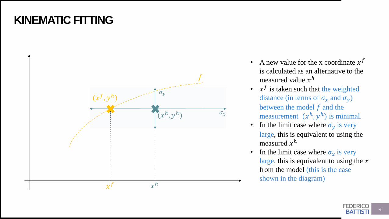
• A new value for the x coordinate 𝑥𝑓
is calculated as an alternative to the
measured value 𝑥ℎ
• 𝑥𝑓 is taken such that the weighted
distance (in terms of 𝜎𝑥 and 𝜎𝑦)
between the model 𝑓 and the
measurement (𝑥ℎ, 𝑦ℎ) is minimal.
• In the limit case where 𝜎𝑦 is very
large, this is equivalent to using the
measured 𝑥ℎ
• In the limit case where 𝜎𝑥 is very
large, this is equivalent to using the 𝑥from the model (this is the case
shown in the diagram)
FEDERICOBATTISTI
KINEMATIC FITTING
5
• Kinematic fitting is an algorithm that updates a measurement within error in the presence of a model
constraint.
• An example of this sort of fit can be found in https://inspirehep.net/literature/1780811 where
kinematic fitting has been used in the context of neutrino-induced charged-current (CC) 𝜋0production on carbon, to improve the neutral pion momentum reconstruction
• For more insights you can consult:
➢ https://www.phys.ufl.edu/~avery/fitting/kinfit_talk1.pdf
➢ http://www-hermes.desy.de/notes/pub/TALK/yaschenk.ColloqGlasgow.pdf

FEDERICOBATTISTI
KALMAN FILTER
6
FEDERICOBATTISTI
KALMAN FILTER IN GENERAL
7
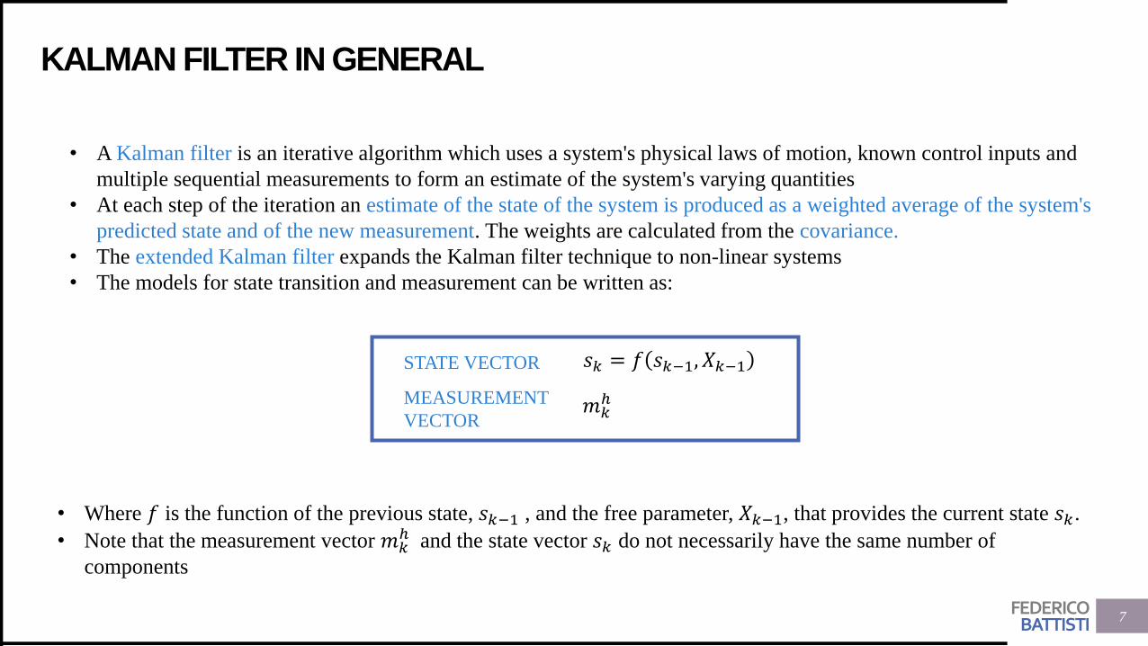
• A Kalman filter is an iterative algorithm which uses a system's physical laws of motion, known control inputs and
multiple sequential measurements to form an estimate of the system's varying quantities
• At each step of the iteration an estimate of the state of the system is produced as a weighted average of the system's
predicted state and of the new measurement. The weights are calculated from the covariance.
• The extended Kalman filter expands the Kalman filter technique to non-linear systems
• The models for state transition and measurement can be written as:
𝑠𝑘 = 𝑓 𝑠𝑘−1, 𝑋𝑘−1
• Where 𝑓 is the function of the previous state, 𝑠𝑘−1 , and the free parameter, 𝑋𝑘−1, that provides the current state 𝑠𝑘.
• Note that the measurement vector 𝑚𝑘ℎ and the state vector 𝑠𝑘 do not necessarily have the same number of
components
𝑚𝑘ℎ
STATE VECTOR
MEASUREMENT
VECTOR
FEDERICOBATTISTI
KALMAN FILTER IN GENERAL
8
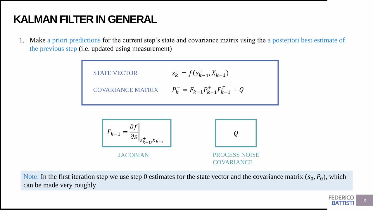
1. Make a priori predictions for the current step’s state and covariance matrix using the a posteriori best estimate of
the previous step (i.e. updated using measurement)
𝑠𝑘− = 𝑓 𝑠𝑘−1
+ , 𝑋𝑘−1
𝑃𝑘− = 𝐹𝑘−1𝑃𝑘−1
+ 𝐹𝑘−1𝑇 + 𝑄
𝐹𝑘−1 = ቤ𝜕𝑓
𝜕𝑠𝑠𝑘−1+ ,𝑋𝑘−1
𝑄
JACOBIAN PROCESS NOISE
COVARIANCE
STATE VECTOR
COVARIANCE MATRIX
Note: In the first iteration step we use step 0 estimates for the state vector and the covariance matrix (𝑠0, 𝑃0), which
can be made very roughly
FEDERICOBATTISTI
KALMAN FILTER IN GENERAL
9
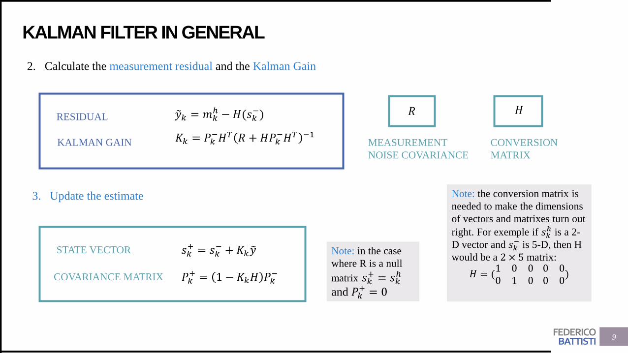
2. Calculate the measurement residual and the Kalman Gain
𝑦𝑘 = 𝑚𝑘ℎ − 𝐻(𝑠𝑘
−)
𝐾𝑘 = 𝑃𝑘−𝐻𝑇 𝑅 + 𝐻𝑃𝑘
−𝐻𝑇 −1
3. Update the estimate
𝑠𝑘+ = 𝑠𝑘
− + 𝐾𝑘 𝑦
𝑃𝑘+ = 1 − 𝐾𝑘𝐻 𝑃𝑘
−
RESIDUAL
KALMAN GAIN
STATE VECTOR
COVARIANCE MATRIX
𝑅
MEASUREMENT
NOISE COVARIANCE
𝐻
CONVERSION
MATRIX
Note: the conversion matrix is
needed to make the dimensions
of vectors and matrixes turn out
right. For exemple if 𝑠𝑘ℎ is a 2-
D vector and 𝑠𝑘− is 5-D, then H
would be a 2 × 5 matrix:
𝐻 = (1 0 00 1 0
0 00 0
)
Note: in the case
where R is a null
matrix 𝑠𝑘+ = 𝑠𝑘
ℎ
and 𝑃𝑘+ = 0
FEDERICOBATTISTI
KALMAN FILTER IN GENERAL
10
(𝑥0ℎ, 𝑦0
ℎ)
(𝑥1ℎ, 𝑦1
−)
(𝑥1ℎ, 𝑦1
ℎ)
(𝑥1ℎ, 𝑦1
+)
(𝑥2ℎ, 𝑦2
+)
(𝑥2ℎ, 𝑦2
−) (𝑥3ℎ, 𝑦3
ℎ) (𝑥4ℎ, 𝑦4
ℎ)
(𝑥3ℎ, 𝑦3
+) (𝑥4ℎ, 𝑦4
+)
(𝑥2ℎ, 𝑦2
ℎ) (𝑥3ℎ, 𝑦3
−)(𝑥4
ℎ, 𝑦4−)
𝑥
𝑦
𝑥1ℎ 𝑥2
ℎ 𝑥4ℎ𝑥3
ℎ

FEDERICOBATTISTI
OUR RECONSTRUCTION ALGORITHM™
11
T. Junk, DUNE-Doc-13933: https://docs.dunescience.org/cgi-bin/private/ShowDocument?docid=13933
FEDERICOBATTISTI
KINEMATIC FITTING
12
𝑑𝑥1
𝑥1ℎ𝑥1
𝑓
(𝑥1ℎ, 𝑦1
ℎ)
𝑓
(𝑥0𝑓, 𝑦0
𝑓)
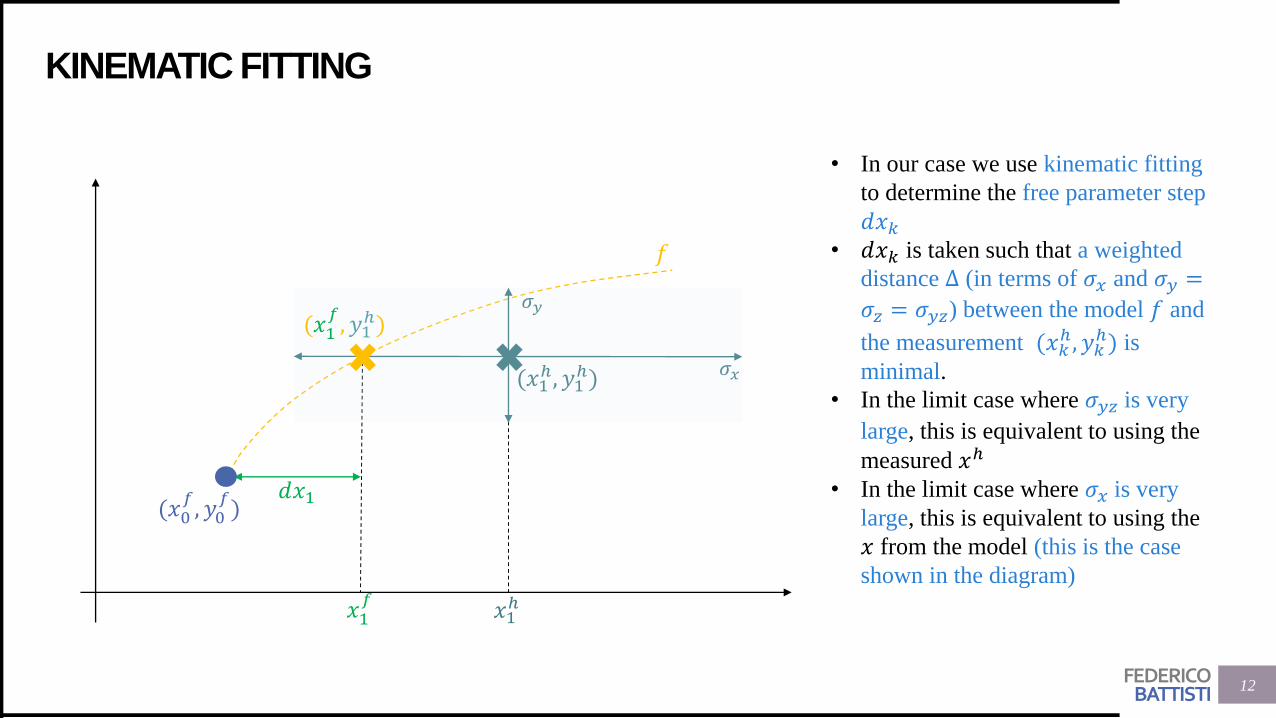
• In our case we use kinematic fitting
to determine the free parameter step
𝑑𝑥𝑘• 𝑑𝑥𝑘 is taken such that a weighted
distance Δ (in terms of 𝜎𝑥 and 𝜎𝑦 =
𝜎𝑧 = 𝜎𝑦𝑧) between the model 𝑓 and
the measurement (𝑥𝑘ℎ, 𝑦𝑘
ℎ) is
minimal.
• In the limit case where 𝜎𝑦𝑧 is very
large, this is equivalent to using the
measured 𝑥ℎ
• In the limit case where 𝜎𝑥 is very
large, this is equivalent to using the
𝑥 from the model (this is the case
shown in the diagram)
𝜎𝑦
𝜎𝑥
(𝑥1𝑓, 𝑦1
ℎ)
FEDERICOBATTISTI
KINEMATIC FITTING
13
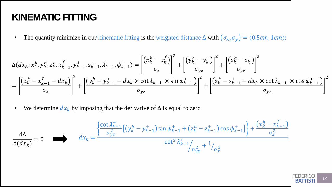
• The quantity minimize in our kinematic fitting is the weighted distance Δ with 𝜎𝑥, 𝜎𝑦 = (0.5𝑐𝑚, 1𝑐𝑚):
Δ(𝑑𝑥𝑘; 𝑥𝑘ℎ, 𝑦𝑘
ℎ, 𝑧𝑘ℎ, 𝑥𝑘−1
𝑓, 𝑦𝑘−1
+ , 𝑧𝑘−1+ , 𝜆𝑘−1
+ , 𝜙𝑘−1+ ) =
𝑥𝑘ℎ − 𝑥𝑘
𝑓
𝜎𝑥
2
+𝑦𝑘ℎ − 𝑦𝑘
−
𝜎𝑦𝑧
2
+𝑧𝑘ℎ − 𝑧𝑘
−
𝜎𝑦𝑧
2
=𝑥𝑘ℎ − 𝑥𝑘−1
𝑓− 𝑑𝑥𝑘
𝜎𝑥
2
+𝑦𝑘ℎ − 𝑦𝑘−1
+ − 𝑑𝑥𝑘 × cot 𝜆𝑘−1 × sin𝜙𝑘−1+
𝜎𝑦𝑧
2
+𝑧𝑘ℎ − 𝑧𝑘−1
+ − 𝑑𝑥𝑘 × cot 𝜆𝑘−1 × cos𝜙𝑘−1+
𝜎𝑦𝑧
2
• We determine 𝑑𝑥𝑘 by imposing that the derivative of Δ is equal to zero
𝑑𝑥𝑘 =
cot 𝜆𝑘−1+
𝜎𝑦𝑧2 𝑦𝑘
ℎ − 𝑦𝑘−1+ sin𝜙𝑘−1
+ + 𝑧𝑘ℎ − 𝑧𝑘−1
+ cos𝜙𝑘−1+ +
𝑥𝑘ℎ − 𝑥𝑘−1
𝑓
𝜎𝑥2
൘cot2 𝜆𝑘−1
+
𝜎𝑦𝑧2 + ൗ1 𝜎𝑥
2
dΔ
d(𝑑𝑥𝑘)= 0
FEDERICOBATTISTI
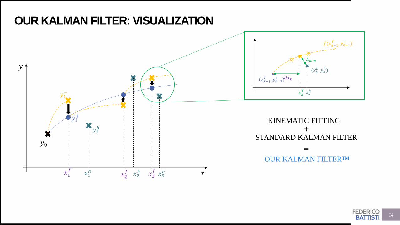
OUR KALMAN FILTER: VISUALIZATION
14
𝑦0
𝑦1−
𝑦1ℎ
𝑦1+
𝑦
𝑥1ℎ 𝑥2
ℎ 𝑥3ℎ𝑥1
𝑓𝑥2𝑓 𝑥3
𝑓
Δ𝑚𝑖𝑛
𝑑𝑥𝑘
𝑥𝑘ℎ𝑥𝑘
𝑓
(𝑥𝑘ℎ , 𝑦𝑘
ℎ)
𝑓(𝑥𝑘−1𝑓
, 𝑦𝑘−1+ )
(𝑥𝑘−1𝑓
, 𝑦𝑘−1+ )
KINEMATIC FITTING
STANDARD KALMAN FILTER
OUR KALMAN FILTER™
+
=
𝑥

FEDERICOBATTISTI
TOY MONTE CARLO STUDY
15
FEDERICOBATTISTI
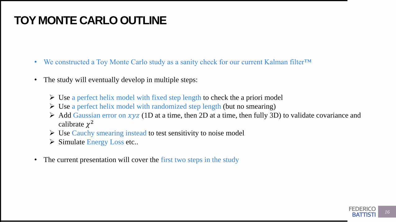
TOY MONTE CARLO OUTLINE
• We constructed a Toy Monte Carlo study as a sanity check for our current Kalman filter™
• The study will eventually develop in multiple steps:
➢ Use a perfect helix model with fixed step length to check the a priori model
➢ Use a perfect helix model with randomized step length (but no smearing)
➢ Add Gaussian error on 𝑥𝑦𝑧 (1D at a time, then 2D at a time, then fully 3D) to validate covariance and
calibrate 𝜒2
➢ Use Cauchy smearing instead to test sensitivity to noise model
➢ Simulate Energy Loss etc..
• The current presentation will cover the first two steps in the study
16
FEDERICOBATTISTI
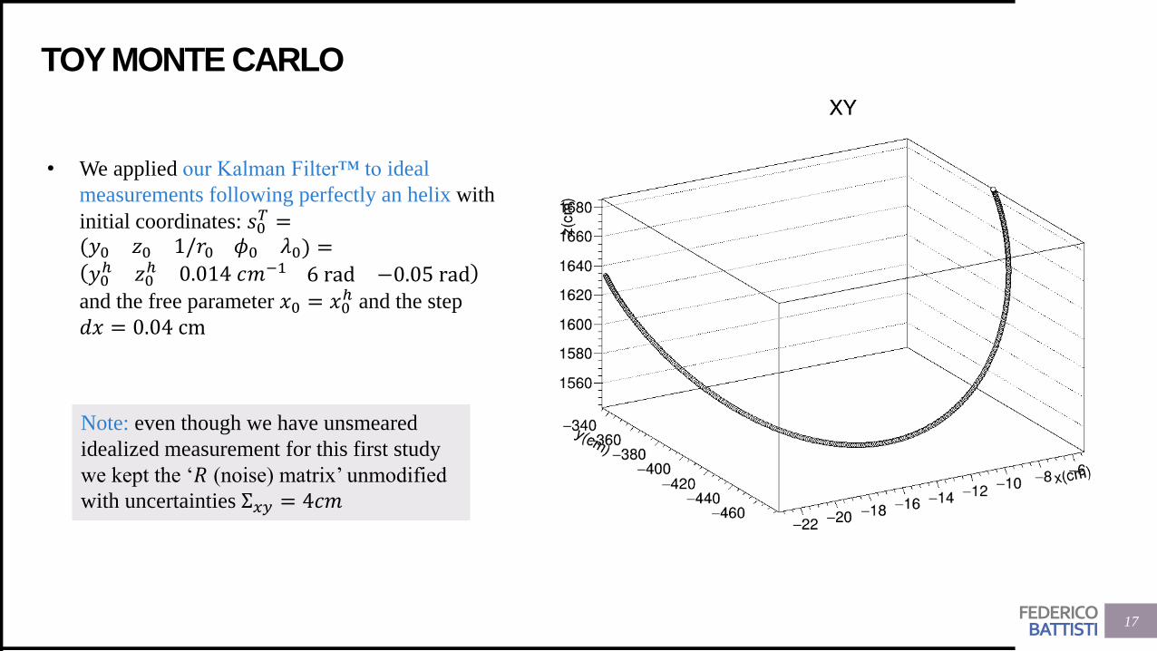
TOY MONTE CARLO
• We applied our Kalman Filter™ to ideal
measurements following perfectly an helix with
initial coordinates: 𝑠0𝑇 =
(𝑦0 𝑧0 1/𝑟0 𝜙0 𝜆0) =𝑦0ℎ 𝑧0
ℎ 0.014 𝑐𝑚−1 6 rad −0.05 radand the free parameter 𝑥0 = 𝑥0
ℎ and the step
𝑑𝑥 = 0.04 cm
17
Note: even though we have unsmeared
idealized measurement for this first study
we kept the ‘𝑅 (noise) matrix’ unmodified
with uncertainties Σ𝑥𝑦 = 4𝑐𝑚
FEDERICOBATTISTI
TOY MONTE CARLO
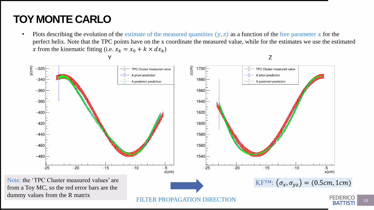
• Plots describing the evolution of the estimate of the measured quantities (𝑦, 𝑧) as a function of the free parameter 𝑥 for the
perfect helix. Note that the TPC points have on the x coordinate the measured value, while for the estimates we use the estimated
𝑥 from the kinematic fitting (i.e. 𝑥𝑘 = 𝑥0 + 𝑘 × 𝑑𝑥𝑘)
18FILTER PROPAGATION DIRECTION
KF™: 𝜎𝑥, 𝜎𝑦𝑧 = (0.5𝑐𝑚, 1𝑐𝑚)Note: the ‘TPC Cluster measured values’ are
from a Toy MC, so the red error bars are the
dummy values from the R matrix
FEDERICOBATTISTI
TOY MONTE CARLO
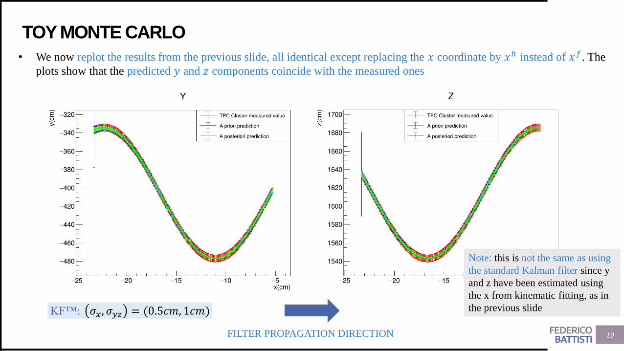
• We now replot the results from the previous slide, all identical except replacing the 𝑥 coordinate by 𝑥ℎ instead of 𝑥𝑓. The
plots show that the predicted 𝑦 and 𝑧 components coincide with the measured ones
19FILTER PROPAGATION DIRECTION
Note: this is not the same as using
the standard Kalman filter since y
and z have been estimated using
the x from kinematic fitting, as in
the previous slideKF™: 𝜎𝑥, 𝜎𝑦𝑧 = (0.5𝑐𝑚, 1𝑐𝑚)
FEDERICOBATTISTI
TOY MONTE CARLO: UNDERSTANDING STEP DETERMINATION
20
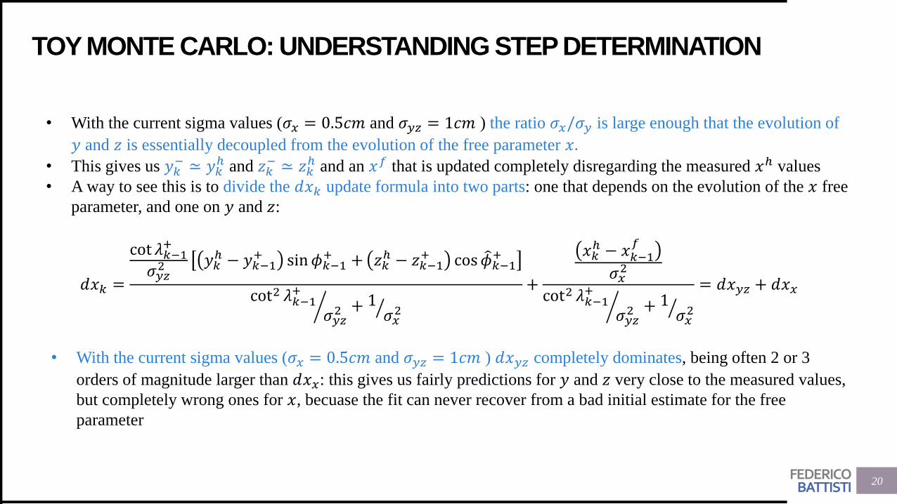
• With the current sigma values (𝜎𝑥 = 0.5𝑐𝑚 and 𝜎𝑦𝑧 = 1𝑐𝑚 ) the ratio 𝜎𝑥/𝜎𝑦 is large enough that the evolution of
𝑦 and 𝑧 is essentially decoupled from the evolution of the free parameter 𝑥.
• This gives us 𝑦𝑘− ≃ 𝑦𝑘
ℎ and 𝑧𝑘− ≃ 𝑧𝑘
ℎ and an 𝑥𝑓 that is updated completely disregarding the measured 𝑥ℎ values
• A way to see this is to divide the 𝑑𝑥𝑘 update formula into two parts: one that depends on the evolution of the 𝑥 free
parameter, and one on 𝑦 and 𝑧:
𝑑𝑥𝑘 =
cot 𝜆𝑘−1+
𝜎𝑦𝑧2 𝑦𝑘
ℎ − 𝑦𝑘−1+ sin𝜙𝑘−1
+ + 𝑧𝑘ℎ − 𝑧𝑘−1
+ cos 𝜙𝑘−1+
൘cot2 𝜆𝑘−1
+
𝜎𝑦𝑧2 + ൗ1 𝜎𝑥
2
+
𝑥𝑘ℎ − 𝑥𝑘−1
𝑓
𝜎𝑥2
൘cot2 𝜆𝑘−1
+
𝜎𝑦𝑧2 + ൗ1 𝜎𝑥
2
= 𝑑𝑥𝑦𝑧 + 𝑑𝑥𝑥
• With the current sigma values (𝜎𝑥 = 0.5𝑐𝑚 and 𝜎𝑦𝑧 = 1𝑐𝑚 ) 𝑑𝑥𝑦𝑧 completely dominates, being often 2 or 3
orders of magnitude larger than 𝑑𝑥𝑥: this gives us fairly predictions for 𝑦 and 𝑧 very close to the measured values,
but completely wrong ones for 𝑥, becuase the fit can never recover from a bad initial estimate for the free
parameter
FEDERICOBATTISTI
TOY MONTE CARLO: UNDERSTANDING STEP DETERMINATION
21FILTER PROPAGATION DIRECTION
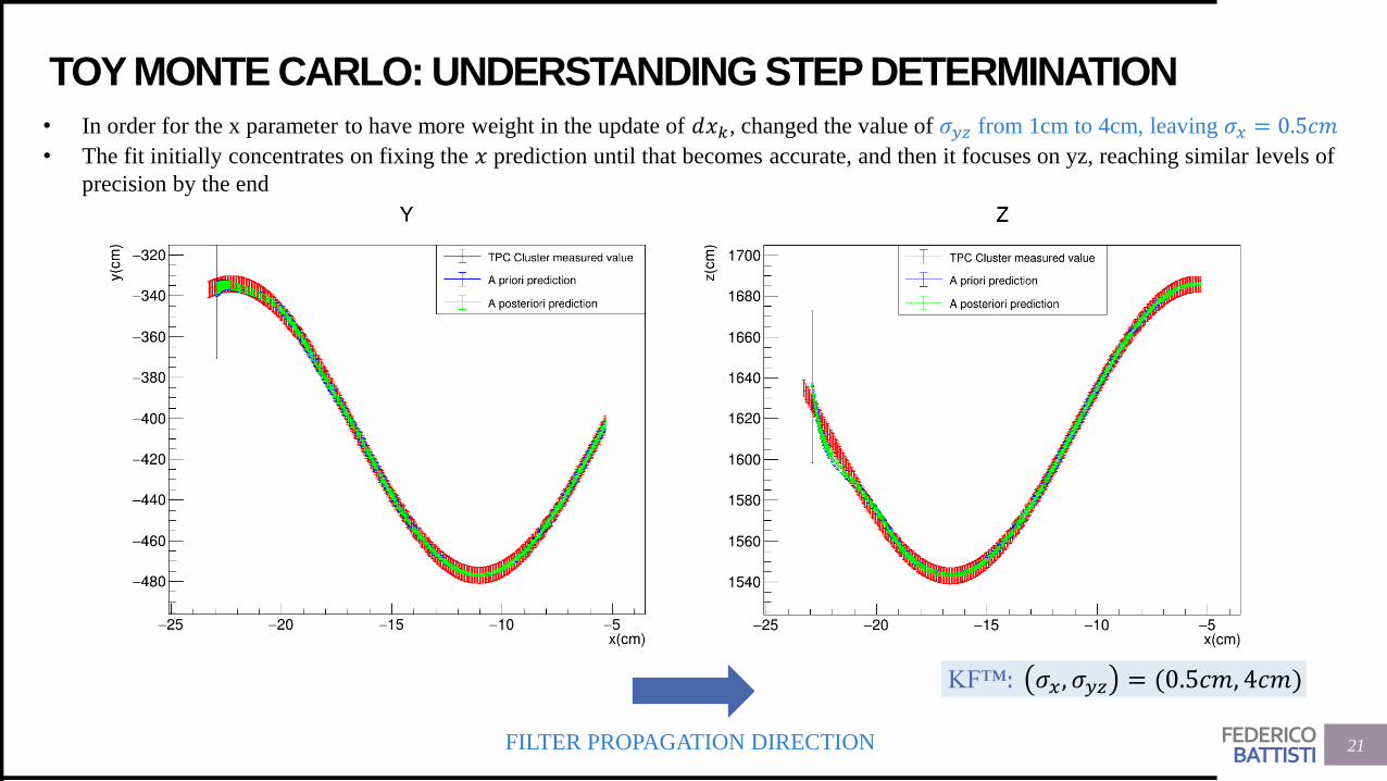
• In order for the x parameter to have more weight in the update of 𝑑𝑥𝑘, changed the value of 𝜎𝑦𝑧 from 1cm to 4cm, leaving 𝜎𝑥 = 0.5𝑐𝑚
• The fit initially concentrates on fixing the 𝑥 prediction until that becomes accurate, and then it focuses on yz, reaching similar levels of
precision by the end
KF™: 𝜎𝑥, 𝜎𝑦𝑧 = (0.5𝑐𝑚, 4𝑐𝑚)
FEDERICOBATTISTI
TOY MONTE CARLO: UNDERSTANDING STEP DETERMINATION
22FILTER PROPAGATION DIRECTION
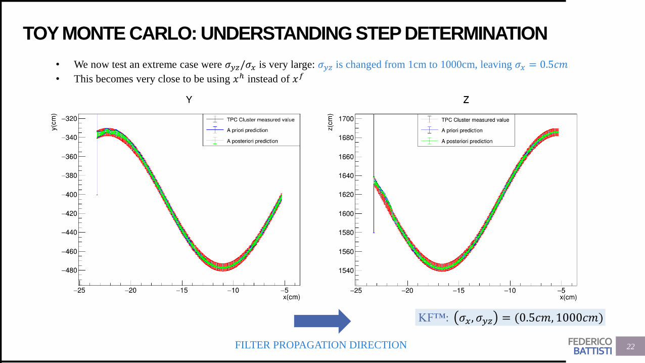
• We now test an extreme case were 𝜎𝑦𝑧/𝜎𝑥 is very large: 𝜎𝑦𝑧 is changed from 1cm to 1000cm, leaving 𝜎𝑥 = 0.5𝑐𝑚
• This becomes very close to be using 𝑥ℎ instead of 𝑥𝑓
KF™: 𝜎𝑥, 𝜎𝑦𝑧 = (0.5𝑐𝑚, 1000𝑐𝑚)
FEDERICOBATTISTI
TOY MONTE CARLO: UNDERSTANDING STEP DETERMINATION
23FILTER PROPAGATION DIRECTION
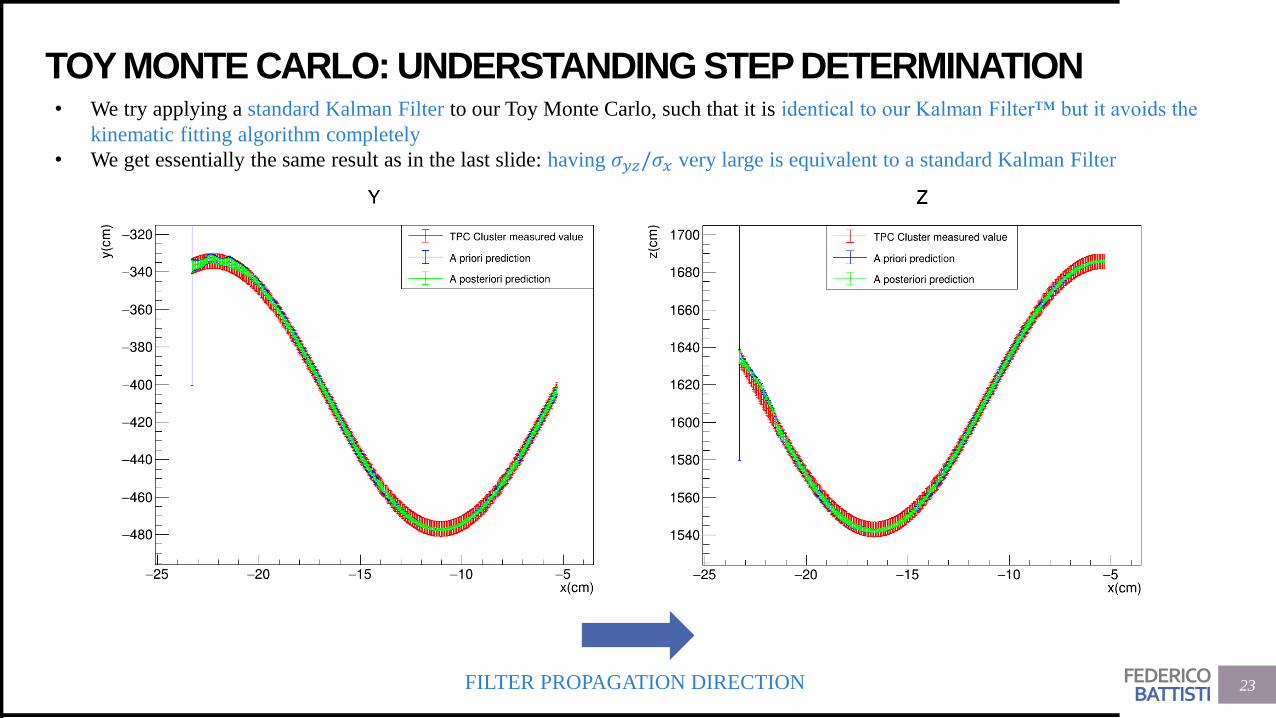
• We try applying a standard Kalman Filter to our Toy Monte Carlo, such that it is identical to our Kalman Filter™ but it avoids the
kinematic fitting algorithm completely
• We get essentially the same result as in the last slide: having 𝜎𝑦𝑧/𝜎𝑥 very large is equivalent to a standard Kalman Filter
FEDERICOBATTISTI
RANDOMIZED X STEP
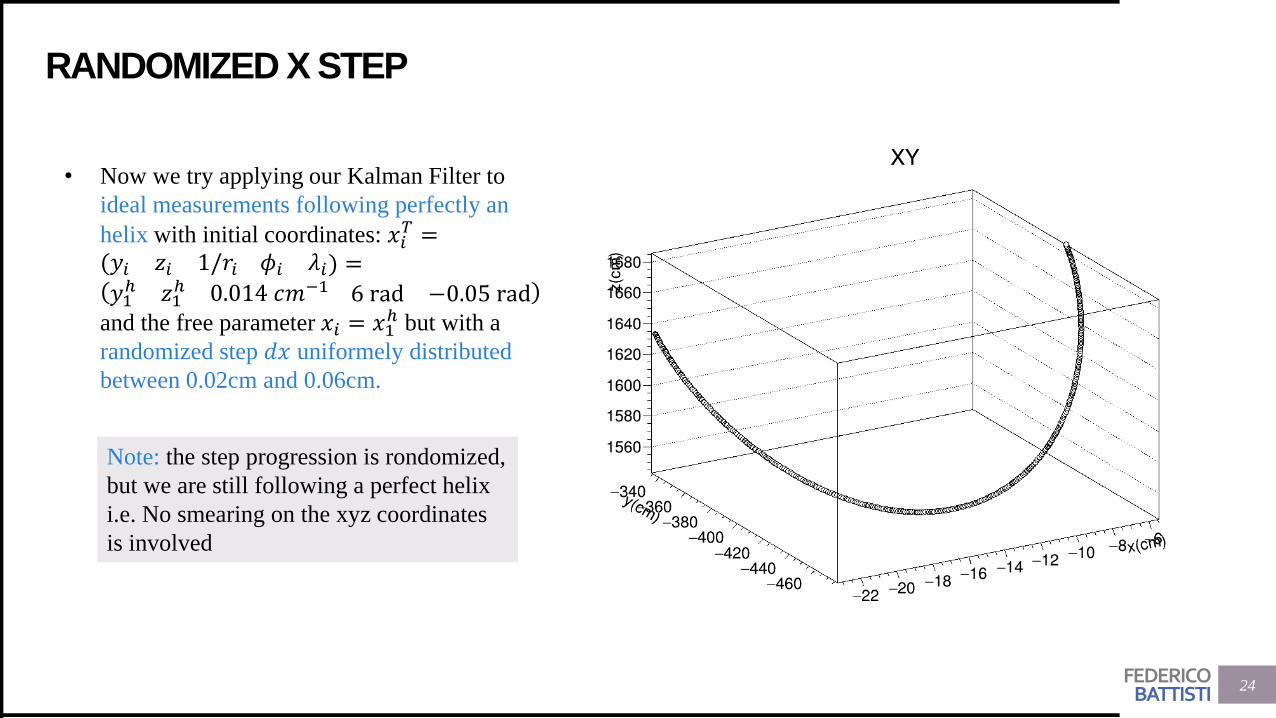
• Now we try applying our Kalman Filter to
ideal measurements following perfectly an
helix with initial coordinates: 𝑥𝑖𝑇 =
(𝑦𝑖 𝑧𝑖 1/𝑟𝑖 𝜙𝑖 𝜆𝑖) =𝑦1ℎ 𝑧1
ℎ 0.014 𝑐𝑚−1 6 rad −0.05 radand the free parameter 𝑥𝑖 = 𝑥1
ℎ but with a
randomized step 𝑑𝑥 uniformely distributed
between 0.02cm and 0.06cm.
24
Note: the step progression is rondomized,
but we are still following a perfect helix
i.e. No smearing on the xyz coordinates
is involved
FEDERICOBATTISTI
RANDOMIZED X STEP
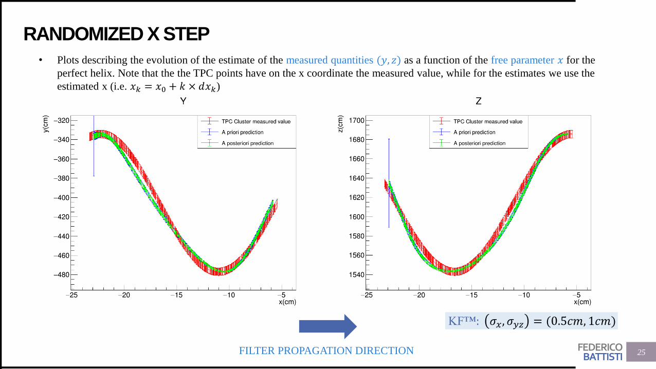
• Plots describing the evolution of the estimate of the measured quantities (𝑦, 𝑧) as a function of the free parameter 𝑥 for the
perfect helix. Note that the the TPC points have on the x coordinate the measured value, while for the estimates we use the
estimated x (i.e. 𝑥𝑘 = 𝑥0 + 𝑘 × 𝑑𝑥𝑘)
25FILTER PROPAGATION DIRECTION
KF™: 𝜎𝑥, 𝜎𝑦𝑧 = (0.5𝑐𝑚, 1𝑐𝑚)
FEDERICOBATTISTI
RANDOMIZED X STEP
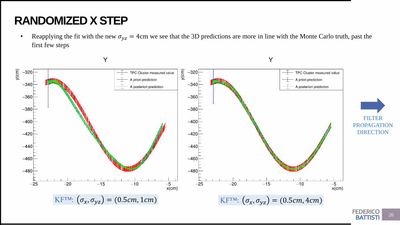
• Reapplying the fit with the new 𝜎𝑦𝑧 = 4cm we see that the 3D predictions are more in line with the Monte Carlo truth, past the
first few steps
26
FILTER
PROPAGATION
DIRECTION
KF™: 𝜎𝑥, 𝜎𝑦𝑧 = (0.5𝑐𝑚, 1𝑐𝑚) KF™: 𝜎𝑥, 𝜎𝑦𝑧 = (0.5𝑐𝑚, 4𝑐𝑚)
FEDERICOBATTISTI
RANDOMIZED X STEP
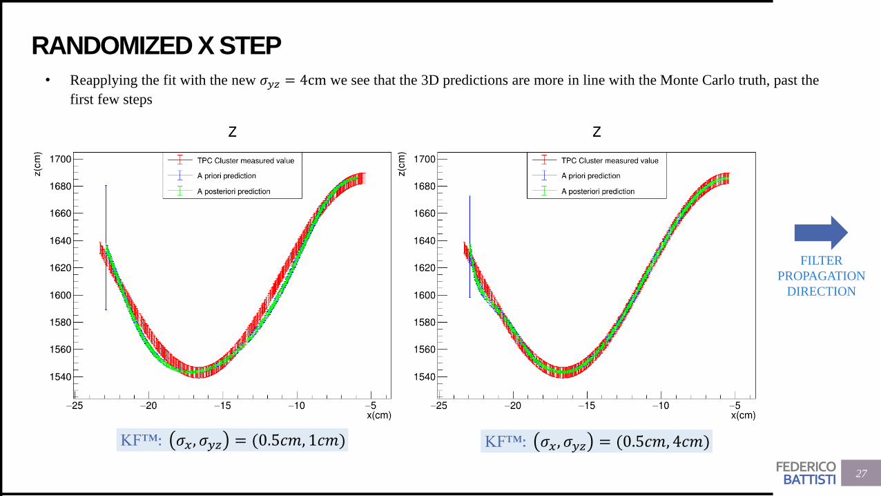
• Reapplying the fit with the new 𝜎𝑦𝑧 = 4cm we see that the 3D predictions are more in line with the Monte Carlo truth, past the
first few steps
27
FILTER
PROPAGATION
DIRECTION
KF™: 𝜎𝑥, 𝜎𝑦𝑧 = (0.5𝑐𝑚, 1𝑐𝑚) KF™: 𝜎𝑥, 𝜎𝑦𝑧 = (0.5𝑐𝑚, 4𝑐𝑚)
FEDERICOBATTISTI
RANDOMIZED X STEP: TESTING THE RATIO
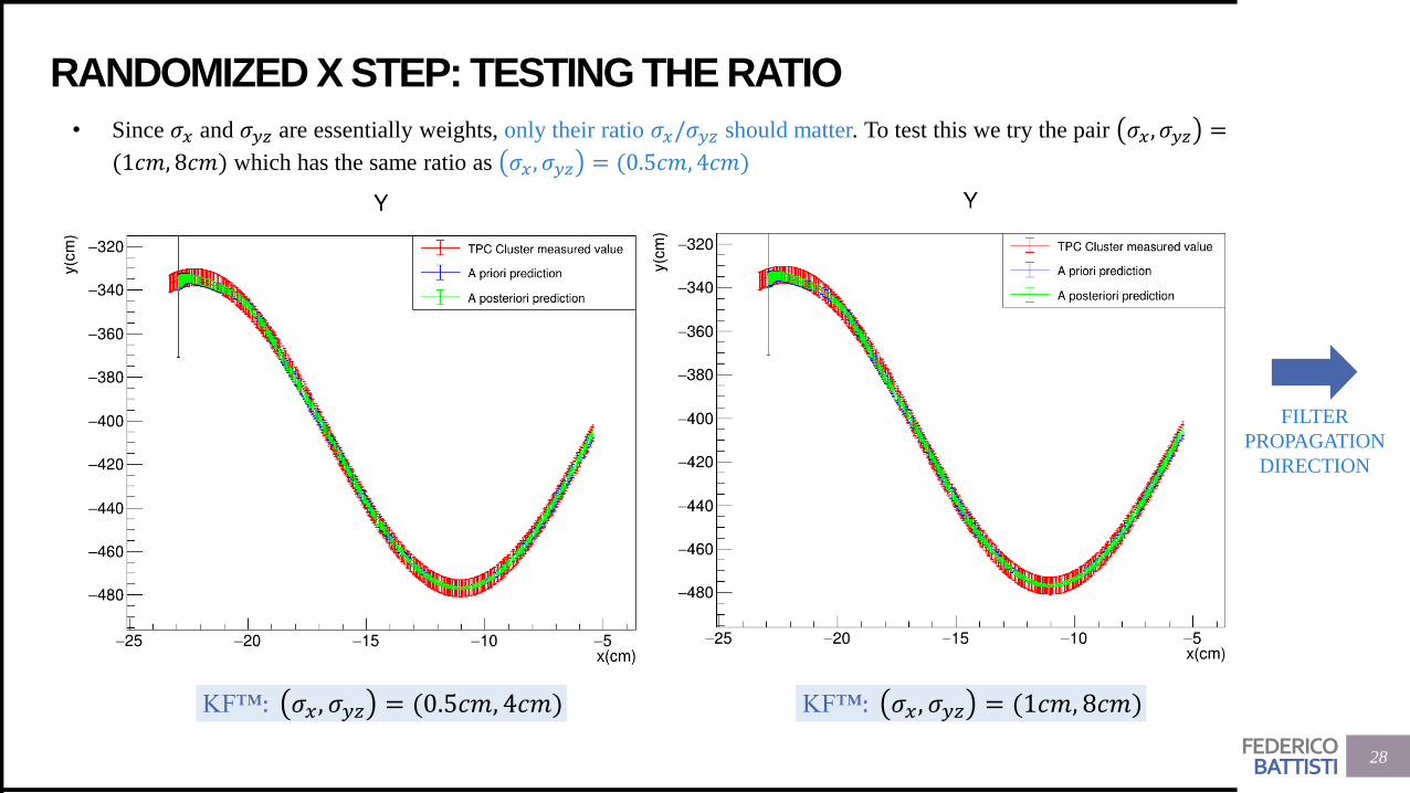
• Since 𝜎𝑥 and 𝜎𝑦𝑧 are essentially weights, only their ratio 𝜎𝑥/𝜎𝑦𝑧 should matter. To test this we try the pair 𝜎𝑥 , 𝜎𝑦𝑧 =
(1𝑐𝑚, 8𝑐𝑚) which has the same ratio as 𝜎𝑥 , 𝜎𝑦𝑧 = (0.5𝑐𝑚, 4𝑐𝑚)
28
FILTER
PROPAGATION
DIRECTION
KF™: 𝜎𝑥, 𝜎𝑦𝑧 = (1𝑐𝑚, 8𝑐𝑚)KF™: 𝜎𝑥, 𝜎𝑦𝑧 = (0.5𝑐𝑚, 4𝑐𝑚)
FEDERICOBATTISTI
RANDOMIZED X STEP: TESTING THE RATIO
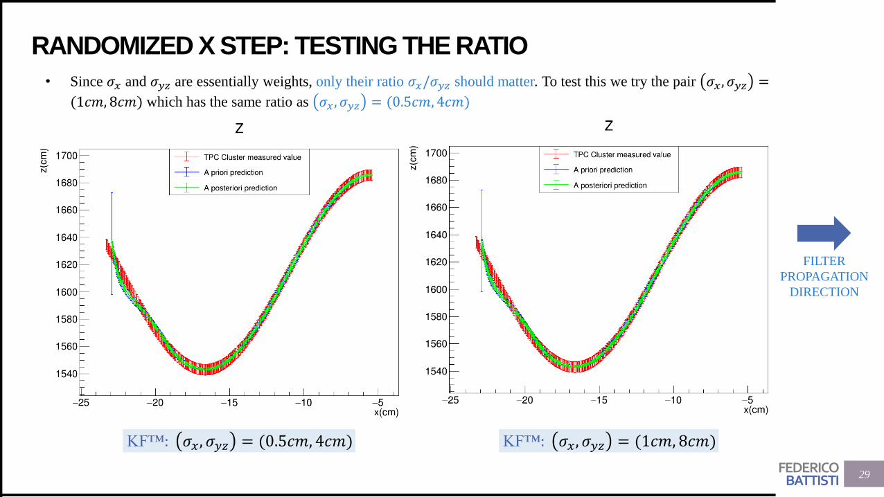
• Since 𝜎𝑥 and 𝜎𝑦𝑧 are essentially weights, only their ratio 𝜎𝑥/𝜎𝑦𝑧 should matter. To test this we try the pair 𝜎𝑥 , 𝜎𝑦𝑧 =
(1𝑐𝑚, 8𝑐𝑚) which has the same ratio as 𝜎𝑥 , 𝜎𝑦𝑧 = (0.5𝑐𝑚, 4𝑐𝑚)
29
FILTER
PROPAGATION
DIRECTION
KF™: 𝜎𝑥, 𝜎𝑦𝑧 = (0.5𝑐𝑚, 4𝑐𝑚) KF™: 𝜎𝑥, 𝜎𝑦𝑧 = (1𝑐𝑚, 8𝑐𝑚)
FEDERICOBATTISTI
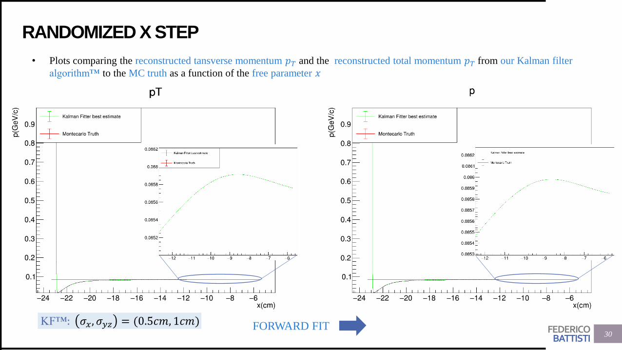
RANDOMIZED X STEP
• Plots comparing the reconstructed tansverse momentum 𝑝𝑇 and the reconstructed total momentum 𝑝𝑇 from our Kalman filter
algorithm™ to the MC truth as a function of the free parameter 𝑥
30FORWARD FITKF™: 𝜎𝑥, 𝜎𝑦𝑧 = (0.5𝑐𝑚, 1𝑐𝑚)
FEDERICOBATTISTI
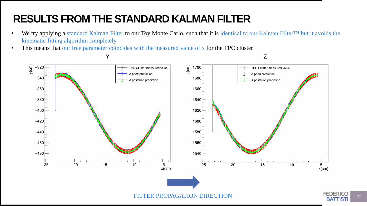
RESULTS FROM THE STANDARD KALMAN FILTER
31FITTER PROPAGATION DIRECTION
• We try applying a standard Kalman Filter to our Toy Monte Carlo, such that it is identical to our Kalman Filter™ but it avoids the
kinematic fitting algorithm completely
• This means that our free parameter coincides with the measured value of x for the TPC cluster
FEDERICOBATTISTI
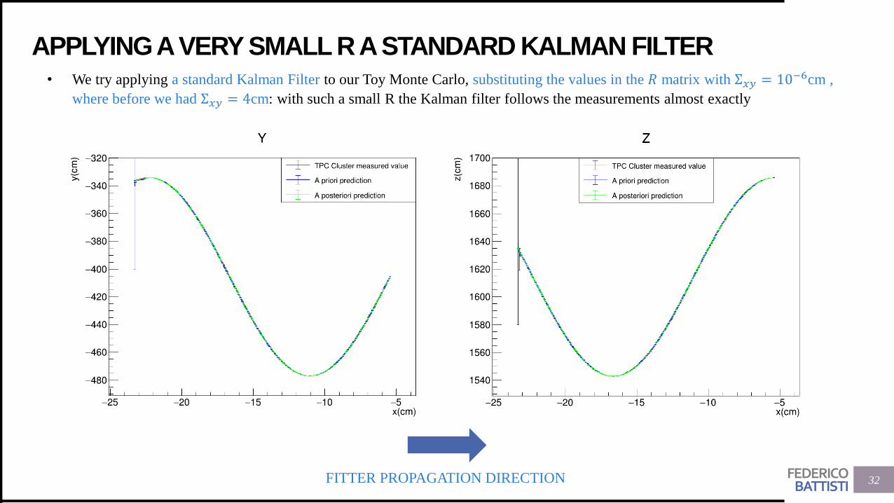
APPLYING A VERY SMALL R A STANDARD KALMAN FILTER
32FITTER PROPAGATION DIRECTION
• We try applying a standard Kalman Filter to our Toy Monte Carlo, substituting the values in the 𝑅 matrix with Σ𝑥𝑦 = 10−6cm ,
where before we had Σ𝑥𝑦 = 4cm: with such a small R the Kalman filter follows the measurements almost exactly
FEDERICOBATTISTI
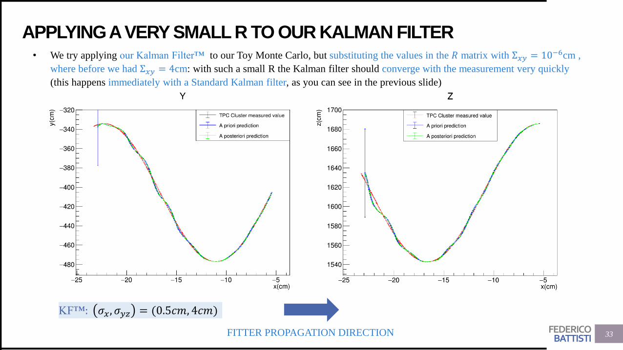
APPLYING A VERY SMALL R TO OUR KALMAN FILTER
33FITTER PROPAGATION DIRECTION
• We try applying our Kalman Filter™ to our Toy Monte Carlo, but substituting the values in the 𝑅 matrix with Σ𝑥𝑦 = 10−6cm ,
where before we had Σ𝑥𝑦 = 4cm: with such a small R the Kalman filter should converge with the measurement very quickly
(this happens immediately with a Standard Kalman filter, as you can see in the previous slide)
KF™: 𝜎𝑥, 𝜎𝑦𝑧 = (0.5𝑐𝑚, 4𝑐𝑚)
FEDERICOBATTISTI
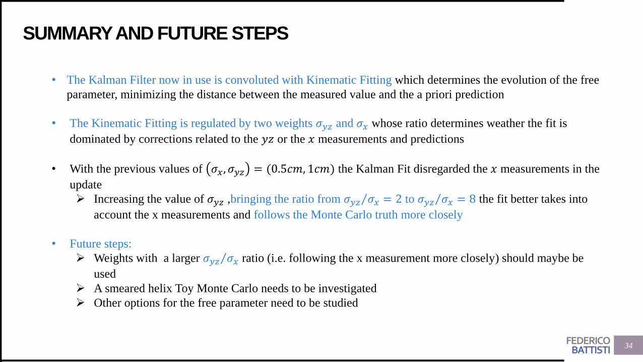
SUMMARY AND FUTURE STEPS
• The Kalman Filter now in use is convoluted with Kinematic Fitting which determines the evolution of the free
parameter, minimizing the distance between the measured value and the a priori prediction
• The Kinematic Fitting is regulated by two weights 𝜎𝑦𝑧 and 𝜎𝑥 whose ratio determines weather the fit is
dominated by corrections related to the 𝑦𝑧 or the 𝑥 measurements and predictions
• With the previous values of 𝜎𝑥, 𝜎𝑦𝑧 = (0.5𝑐𝑚, 1𝑐𝑚) the Kalman Fit disregarded the 𝑥 measurements in the
update
➢ Increasing the value of 𝜎𝑦𝑧 ,bringing the ratio from Τ𝜎𝑦𝑧 𝜎𝑥 = 2 to Τ𝜎𝑦𝑧 𝜎𝑥 = 8 the fit better takes into
account the x measurements and follows the Monte Carlo truth more closely
• Future steps:
➢ Weights with a larger Τ𝜎𝑦𝑧 𝜎𝑥 ratio (i.e. following the x measurement more closely) should maybe be
used
➢ A smeared helix Toy Monte Carlo needs to be investigated
➢ Other options for the free parameter need to be studied
34

FEDERICOBATTISTI
BACKUP
35
FEDERICOBATTISTI
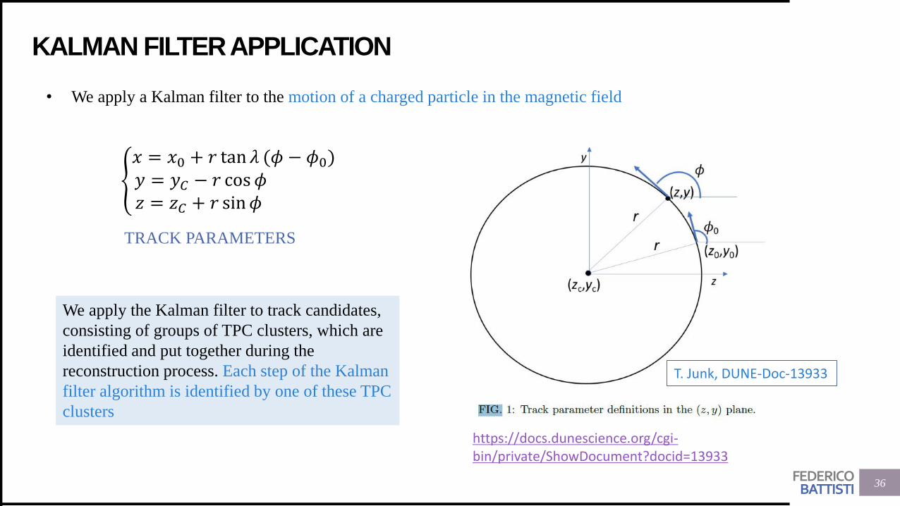
KALMAN FILTER APPLICATION
36
• We apply a Kalman filter to the motion of a charged particle in the magnetic field
ቐ
𝑥 = 𝑥0 + 𝑟 tan𝜆 (𝜙 − 𝜙0)𝑦 = 𝑦𝐶 − 𝑟 cos𝜙𝑧 = 𝑧𝐶 + 𝑟 sin𝜙
TRACK PARAMETERS
We apply the Kalman filter to track candidates,
consisting of groups of TPC clusters, which are
identified and put together during the
reconstruction process. Each step of the Kalman
filter algorithm is identified by one of these TPC
clusters
T. Junk, DUNE-Doc-13933
https://docs.dunescience.org/cgi-bin/private/ShowDocument?docid=13933
FEDERICOBATTISTI
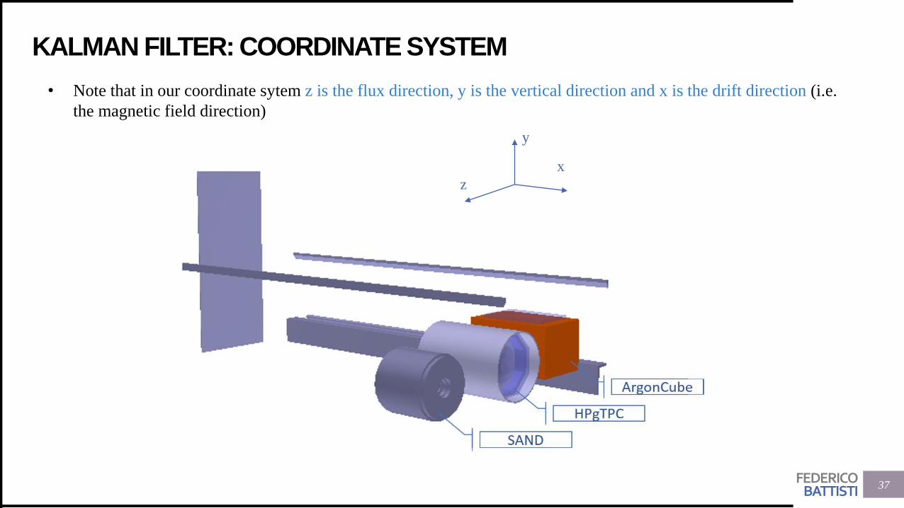
KALMAN FILTER: COORDINATE SYSTEM
37
• Note that in our coordinate sytem z is the flux direction, y is the vertical direction and x is the drift direction (i.e.
the magnetic field direction)
y
z
x
FEDERICOBATTISTI
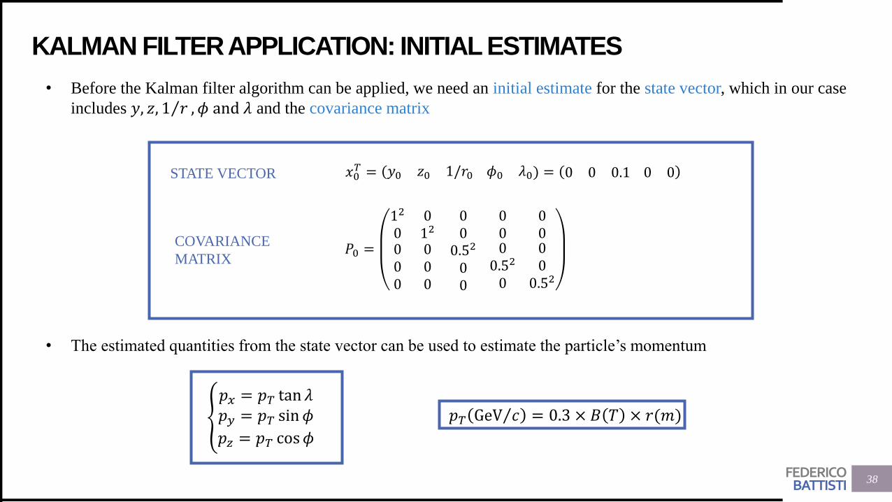
KALMAN FILTER APPLICATION: INITIAL ESTIMATES
• Before the Kalman filter algorithm can be applied, we need an initial estimate for the state vector, which in our case
includes 𝑦, 𝑧, Τ1 𝑟 , 𝜙 and 𝜆 and the covariance matrix
𝑥0𝑇 = (𝑦0 𝑧0 1/𝑟0 𝜙0 𝜆0) = 0 0 0.1 0 0
𝑃0 =
12 0 00 12 0000
000
0.52
00
000
0.52
0
0000
0.52
STATE VECTOR
COVARIANCE
MATRIX
38
• The estimated quantities from the state vector can be used to estimate the particle’s momentum
൞
𝑝𝑥 = 𝑝𝑇 tan 𝜆𝑝𝑦 = 𝑝𝑇 sin𝜙
𝑝𝑧 = 𝑝𝑇 cos𝜙
𝑝𝑇 ΤGeV 𝑐 = 0.3 × 𝐵 𝑇 × 𝑟(𝑚)
FEDERICOBATTISTI
KALMAN FILTER APPLICATION: PREDICTION AND MEASUREMENT
39
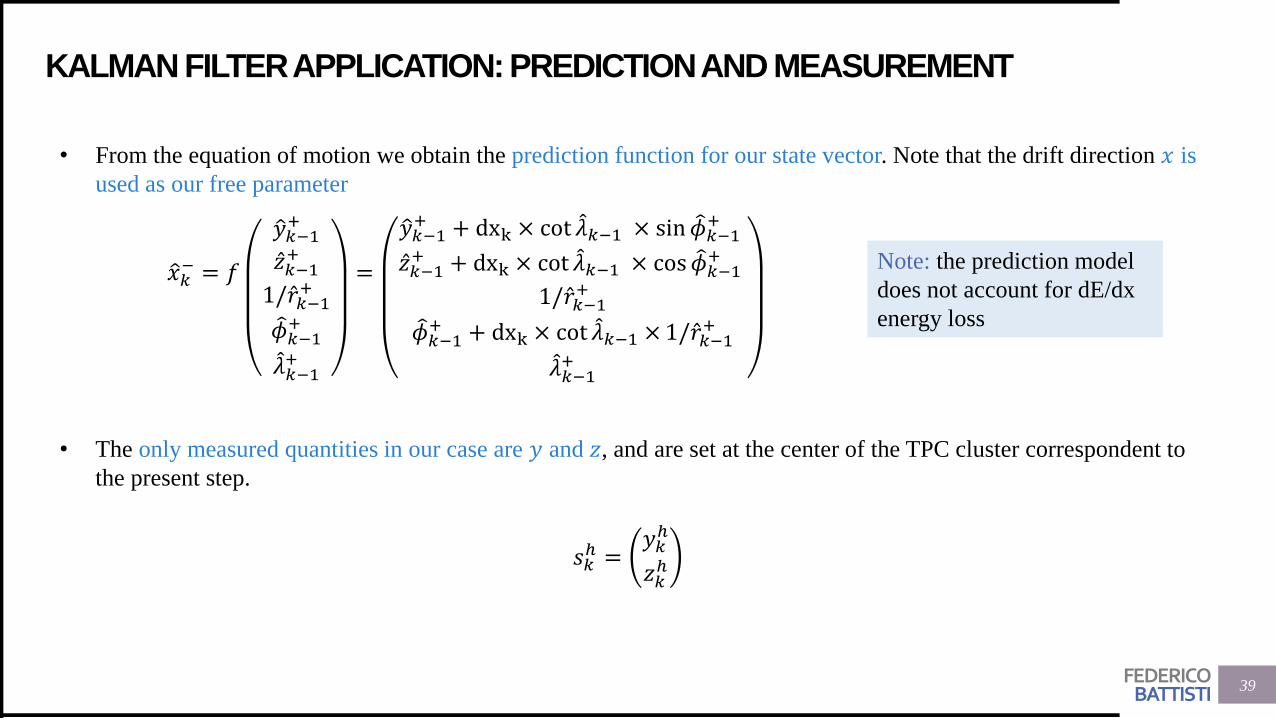
• From the equation of motion we obtain the prediction function for our state vector. Note that the drift direction 𝑥 is
used as our free parameter
ො𝑥𝑘− = 𝑓
ො𝑦𝑘−1+
Ƹ𝑧𝑘−1+
1/ Ƹ𝑟𝑘−1+
𝜙𝑘−1+
መ𝜆𝑘−1+
=
ො𝑦𝑘−1+ + dxk × cot መ𝜆𝑘−1 × sin 𝜙𝑘−1
+
Ƹ𝑧𝑘−1+ + dxk × cot መ𝜆𝑘−1 × cos 𝜙𝑘−1
+
1/ Ƹ𝑟𝑘−1+
𝜙𝑘−1+ + dxk × cot መ𝜆𝑘−1 ×1/ Ƹ𝑟𝑘−1
+
መ𝜆𝑘−1+
• The only measured quantities in our case are 𝑦 and 𝑧, and are set at the center of the TPC cluster correspondent to
the present step.
𝑠𝑘ℎ =
𝑦𝑘ℎ
𝑧𝑘ℎ
Note: the prediction model
does not account for dE/dx
energy loss
FEDERICOBATTISTI
KALMAN FILTER APPLICATION: COVARIANCE MATRIX PREDICTION
40
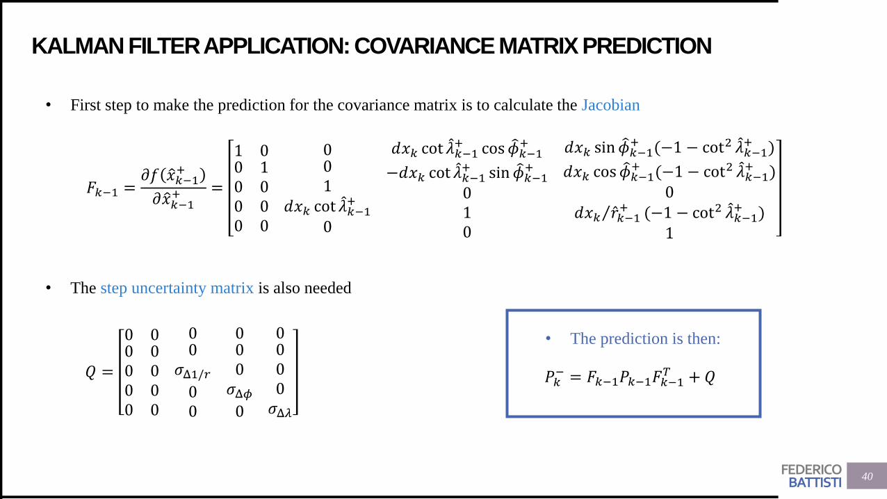
• First step to make the prediction for the covariance matrix is to calculate the Jacobian
𝐹𝑘−1 =𝜕𝑓 ො𝑥𝑘−1
+
𝜕 ො𝑥𝑘−1+ =
1 00000
1000
001
𝑑𝑥𝑘 cot መ𝜆𝑘−1+
0
𝑑𝑥𝑘 cot መ𝜆𝑘−1+ cos 𝜙𝑘−1
+
−𝑑𝑥𝑘 cot መ𝜆𝑘−1+ sin 𝜙𝑘−1
+
010
𝑑𝑥𝑘 sin 𝜙𝑘−1+ (−1 − cot2 መ𝜆𝑘−1
+ )
𝑑𝑥𝑘 cos 𝜙𝑘−1+ (−1 − cot2 መ𝜆𝑘−1
+ )0
Τ𝑑𝑥𝑘 Ƹ𝑟𝑘−1+ (−1 − cot2 መ𝜆𝑘−1
+ )1
• The step uncertainty matrix is also needed
𝑄 =
0 00000
0000
00
𝜎Δ1/𝑟00
000𝜎Δ𝜙0
0000𝜎Δ𝜆
• The prediction is then:
𝑃𝑘− = 𝐹𝑘−1𝑃𝑘−1𝐹𝑘−1
𝑇 + 𝑄
FEDERICOBATTISTI
KALMAN FILTER APPLICATION: EVALUATE THE RESIDUAL
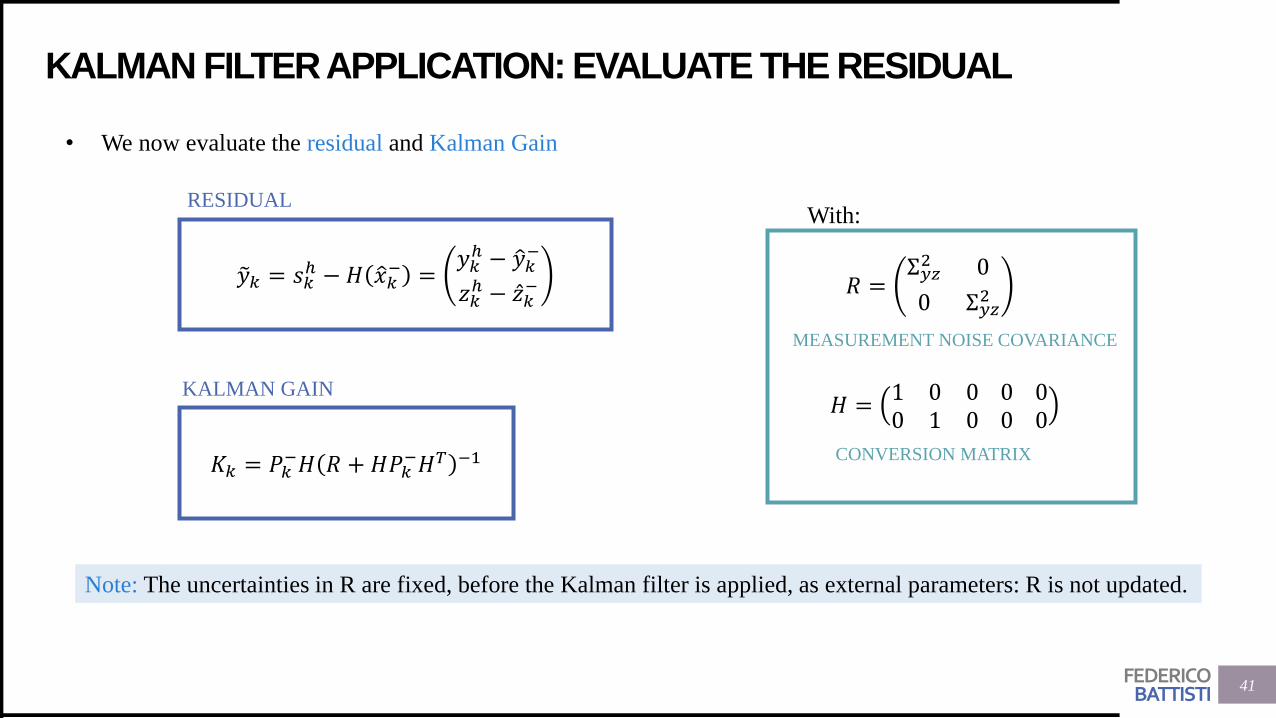
• We now evaluate the residual and Kalman Gain
𝑦𝑘 = 𝑠𝑘ℎ −𝐻 ො𝑥𝑘
− =𝑦𝑘ℎ − ො𝑦𝑘
−
𝑧𝑘ℎ − Ƹ𝑧𝑘
−
𝐾𝑘 = 𝑃𝑘−𝐻 𝑅 + 𝐻𝑃𝑘
−𝐻𝑇 −1
𝐻 =1 0 00 1 0
00
00
𝑅 =Σ𝑦𝑧2 0
0 Σ𝑦𝑧2
KALMAN GAIN
RESIDUAL With:
CONVERSION MATRIX
MEASUREMENT NOISE COVARIANCE
Note: The uncertainties in R are fixed, before the Kalman filter is applied, as external parameters: R is not updated.
41
FEDERICOBATTISTI
KALMAN FILTER APPLICATION: PREDICTION UPDATE
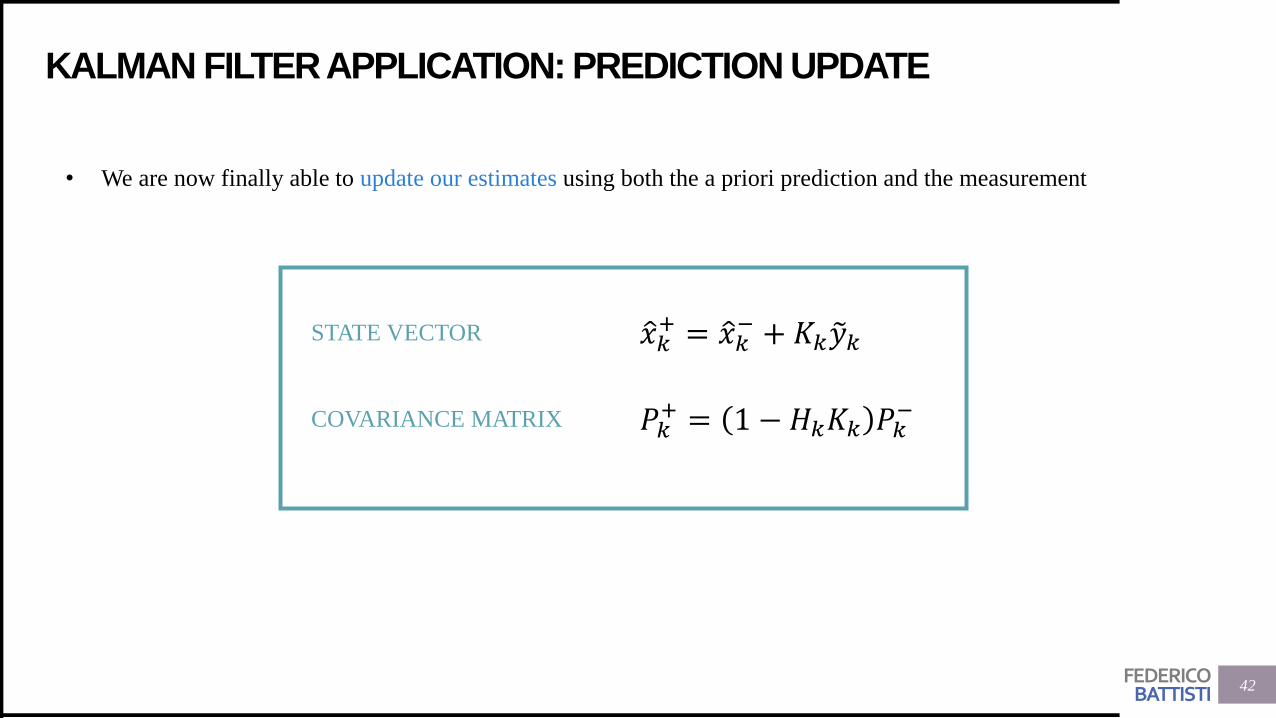
• We are now finally able to update our estimates using both the a priori prediction and the measurement
ො𝑥𝑘+ = ො𝑥𝑘
− + 𝐾𝑘 𝑦𝑘
𝑃𝑘+ = 1 − 𝐻𝑘𝐾𝑘 𝑃𝑘
−
STATE VECTOR
COVARIANCE MATRIX
42
FEDERICOBATTISTI
TOY MONTE CARLO
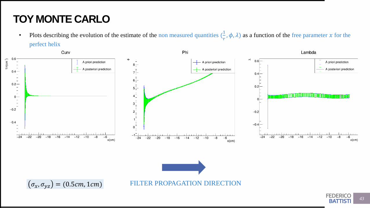
• Plots describing the evolution of the estimate of the non measured quantities (1
𝑟, 𝜙, 𝜆) as a function of the free parameter 𝑥 for the
perfect helix
43
FILTER PROPAGATION DIRECTION
43
𝜎𝑥, 𝜎𝑦𝑧 = (0.5𝑐𝑚, 1𝑐𝑚)
FEDERICOBATTISTI
TOY MONTE CARLO
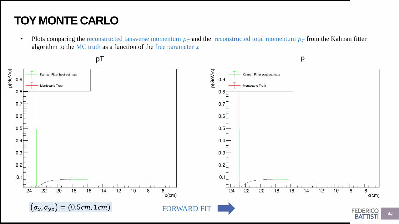
• Plots comparing the reconstructed tansverse momentum 𝑝𝑇 and the reconstructed total momentum 𝑝𝑇 from the Kalman fitter
algorithm to the MC truth as a function of the free parameter 𝑥
44FORWARD FIT𝜎𝑥, 𝜎𝑦𝑧 = (0.5𝑐𝑚, 1𝑐𝑚)
FEDERICOBATTISTI
RANDOMIZED X STEP
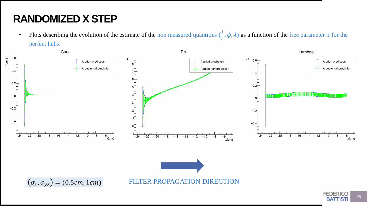
• Plots describing the evolution of the estimate of the non measured quantities (1
𝑟, 𝜙, 𝜆) as a function of the free parameter 𝑥 for the
perfect helix
45
FILTER PROPAGATION DIRECTION
45
𝜎𝑥, 𝜎𝑦𝑧 = (0.5𝑐𝑚, 1𝑐𝑚)
FEDERICOBATTISTI
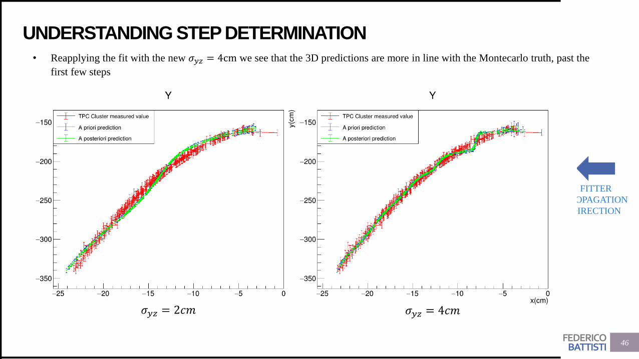
UNDERSTANDING STEP DETERMINATION
• Reapplying the fit with the new 𝜎𝑦𝑧 = 4cm we see that the 3D predictions are more in line with the Montecarlo truth, past the
first few steps
46
FITTER
PROPAGATION
DIRECTION
𝜎𝑦𝑧 = 2𝑐𝑚 𝜎𝑦𝑧 = 4𝑐𝑚
FEDERICOBATTISTI
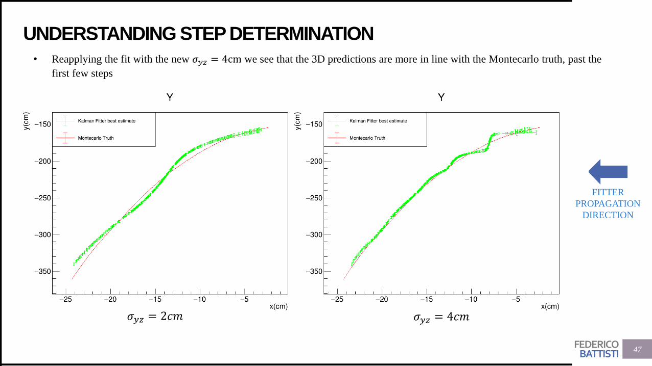
UNDERSTANDING STEP DETERMINATION
• Reapplying the fit with the new 𝜎𝑦𝑧 = 4cm we see that the 3D predictions are more in line with the Montecarlo truth, past the
first few steps
47
𝜎𝑦𝑧 = 2𝑐𝑚
FITTER
PROPAGATION
DIRECTION
𝜎𝑦𝑧 = 4𝑐𝑚

FEDERICOBATTISTI
UNDERSTANDING STEP DETERMINATION
• The momentum reconstruction performance remains roughly the same
48BACKWARD FIT