Universite Paris 7 — Denis DiderotUFR d’Informatique

THESE

pour l’obtention du Diplome deDocteur de l’Universite Paris 7

Specialite Informatique

presentee et soutenue publiquement par

Francesco Zappa Nardelli

le 12 decembre 2003.

De la semantique des processus d’ordre superieur

Directeur de these :Giuseppe Castagna

Jury :

MM. Pierre-Louis Curien President

Giuseppe Castagna

Matthew Hennessy

Jean-Jacques Levy

Glynn Winskel

Rapporteurs :

MM. Matthew Hennessy

Davide Sangiorgi

A big thank you to Giuseppe Castagna for hisguidance during these years, to Matthew Hen-nessy and Davide Sangiorgi for reviewing mythesis, and to all the members of the jury.A big thank you to Giorgio Ghelli.A big thank you to Massimo Merro and GlynnWinskel for their friendship.A big thank you to Jan Vitek, Gergana Mar-kova, Chrislain Razafimahefa, Michel Pawlak.A big thank you to the persons I sharedan house with: Davide Malacaria, AlessandroUrpi, Pio Nardiello in Pisa, without forgettingAlessandro Casanovi; Cecilia Soderlund, NoemiJacobs, and Shams in the most internationalflat I lived in; Marie Coris and Anne-SophiePeyne in Brighton.A big thank you to Amy Clemitshaw and So-phie Maltby for the long walks on Brightonseafront.A big thank you to two great bars: chez Paco(de profundis) in Paris, and the Full Moon inBrighton — thank you, Paul Stones, and all thepoets.A big thank you to an old Fiat 500 (de pro-fundis), to Ernesto Mistretta, to Carlos MunozCamacho.A big thank you to my parents, Giuliana‘mamma’ Nardelli and Paolo ‘babbo’ Zappa. Abig thank you to my friends from Perugia: Da-niele ‘Monta’ Montagnoli, Miriam Menichelli,Marco ‘Basco’ Bastianelli, Lorenzo ‘Merio’ Ma-riani, Marco ’Borgo’ Borghesi, Giacomo Scor-sipa, Stefania Cruciani.A big thank you to the persons I shared an of-fice with: Juliusz Chroboczek, Gabriele Santini,Samuel Hym, Alain Frisch, Jim Laird. And ofcourse Frederic De Jaeger and Cedric Lhouis-sane.A big thank you to Eric Goubault, Vladi-miro Sassone, Giuseppe Longo, Matteo Coccia,Marco Carbone, Sophie Lepine, Tom Hirscho-witz, Marie Duflot, Olivier Glass, Marine Pi-con, Julian Rathke and especially to Katarzina‘Katy’ Wozniak.And the biggest thank you to Annick ‘Piccina’Grandemange.

To The man who killed Don Quijote.

Un grand merci a Giuseppe Castagna pouravoir dirige mes etudes, a Matthew Hennessyet Davide Sangiorgi pour avoir accepte d’etrerapporteurs, a tous les membres du jury.Un grand merci a Giorgio Ghelli.Un grand merci a Massimo Merro et a GlynnWinskel pour leur amitie.Un grand merci a Jan Vitek, Gergana Markova,Chrislain Razafimahefa, Michel Pawlak.Un grand merci aux amis avec lesquels j’ai par-tage une maison : Davide Malacaria, AlessandroUrpi, Pio Nardiello a Pise, sans oublier Ales-sandro Casanovi ; Cecilia Soderlund, Noemi Ja-cobs, et Shams dans l’appartement le plus inter-national au monde ; Marie Coris et Anne-SophiePeyne a Brighton.Un grand merci a Amy Clemitshaw et SophieMaltby pour les longues promenade sur la plagede Brighton.Un grand merci a deux grands bars : chez Paco(de profundis) a Paris, et le Full Moon a Brigh-ton — un grand merci a Paul Stones et a tousles poetes.Un grand merci a une vieille Fiat 500 (de pro-fundis), a Ernesto Mistretta et a Carlos MunozCamacho.Un grand merci a mes parents, Giuliana ‘Mam-ma’ Nardelli et Paolo ‘Babbo’ Zappa. Un grandmerci a mes amis de Perouse : Daniele ‘Mon-ta’ Montagnoli, Miriam Menichelli, Marco ‘Bas-co’ Bastianelli, Lorenzo ‘Merio’ Mariani, Marco’Borgo’ Borghesi, Giacomo Scorsipa, StefaniaCruciani.Un grand merci aux personnes avec lesquellesj’ai partage un bureau : Juliusz Chroboczek,Gabriele Santini, Samuel Hym, Alain Frisch,Jim Laird. Et bien sur Frederic De Jaeger etCedric Lhouissane.Un grand merci a Eric Goubault, Vladi-miro Sassone, Giuseppe Longo, Matteo Coccia,Marco Carbone, Sophie Lepine, Tom Hirscho-witz, Marie Duflot, Olivier Glass, Marine Pi-con, Julian Rathke et surtout a Katarzina ‘Ka-ty’ Wozniak.Et le merci le plus grand est pour Annick ‘Pic-cina’ Grandemange.

A The man who killed Don Quijote.

Contents

1 Resume 7

2 Introduction 472.1 On the semantics of process languages . . . . . . . . . . . . . . . . . . . . . 482.2 A process language out of a semantic model . . . . . . . . . . . . . . . . . . 542.3 Overview . . . . . . . . . . . . . . . . . . . . . . . . . . . . . . . . . . . . . . 57

On the semantics of process languages 59

3 The Seal Calculus 613.1 Syntax and operational semantics . . . . . . . . . . . . . . . . . . . . . . . . 623.2 Behavioural theories . . . . . . . . . . . . . . . . . . . . . . . . . . . . . . . 683.3 A labelled transition semantics . . . . . . . . . . . . . . . . . . . . . . . . . . 703.4 A proof method . . . . . . . . . . . . . . . . . . . . . . . . . . . . . . . . . . 813.5 Algebraic theory . . . . . . . . . . . . . . . . . . . . . . . . . . . . . . . . . 94

4 Mobile Ambients 974.1 Mobile Ambients in two levels . . . . . . . . . . . . . . . . . . . . . . . . . . 984.2 A labelled transition semantics . . . . . . . . . . . . . . . . . . . . . . . . . . 1004.3 Characterising reduction barbed congruence . . . . . . . . . . . . . . . . . . 1074.4 Up-to proof techniques . . . . . . . . . . . . . . . . . . . . . . . . . . . . . . 1334.5 Adding communication . . . . . . . . . . . . . . . . . . . . . . . . . . . . . . 1364.6 Algebraic theory . . . . . . . . . . . . . . . . . . . . . . . . . . . . . . . . . 138

Notes and References 143

A process language out of a semantic model 147

5 new-HOPLA 1495.1 Domain theory for path sets . . . . . . . . . . . . . . . . . . . . . . . . . . . 1505.2 The language . . . . . . . . . . . . . . . . . . . . . . . . . . . . . . . . . . . 1535.3 Equivalences . . . . . . . . . . . . . . . . . . . . . . . . . . . . . . . . . . . . 1685.4 Examples . . . . . . . . . . . . . . . . . . . . . . . . . . . . . . . . . . . . . 178

Notes and References 197

6 Conclusion 199

Bibliography 203

1 Resume

Ce premier chapitre presente de maniere exhaustive la demarche et les resultats des tra-vaux de la presente these. Il ne saurait toutefois constituer qu’un apercu, et nous renvoyons,pour de plus amples details, explications et exemples, et pour toutes les preuves, aux chapitressuivants (2 a 6), rediges en anglais.

Les theories du calcul sequentiel sont essentiellement des theories des fonctions calcu-lables : un programme sequentiel transforme un ensemble de valeurs d’entree en un en-semble de valeurs de sortie, en executant une sequence d’actions mecaniques. L’approchedenotationnelle de Scott et Strachey, par le cadre mathematique general du calcul sequentielqu’elle offre, s’est revelee fondamentale, car elle a ainsi permis, notamment, la comparaisondes langages de programmation, la mise en relation du calcul sequentiel et des domainesmathematiques que sont l’algebre, la topologie et la logique, et la mise au point de nouveauxsystemes de typage, des nouvelles constructions de programmation, et de nouvelles methodesd’analyse des programmes.

Cette approche fonctionnelle du calcul demeure cependant insuffisante pour analyserles systemes concurrents. En effet, dans un systeme concurrent, des agents actifs influencentmutuellement leur action, par des interactions constantes et variees : l’interet de tels systemesreside dans cette interaction, dans le flot de donnees, et pas dans la relation entree-sortie.Ainsi, dans la mesure ou, dans un tel contexte, les analyses de la concurrence ne beneficientpas de la mise au point d’un cadre mathematique global analogue a celui de Scott et Stracheypour le calcul sequentiel, elles prennent d’ordinaire pour objet une notion jugee fondamentale,autour de laquelle un modele est construit, puis teste.

Parmi ces notions, l’existence de « noms », a ete au centre de nombreuses recherches,car celle-ci est inseparable du processus de communication, fondamental dans tout systemeconcurrent. L’existence de noms suggere de plus un espace abstrait de processus connectes,dans lequel les noms representent les connections ; seuls les processus qui partagent desnoms sont alors en mesure d’interagir. La structure d’un systeme change donc de manieredynamique, car les liens entre processus sont sans cesse crees et detruits.

Si cette mobilite des liens est bien connue et analysee, il n’en va pas de meme de lamobilite des processus au sein de l’espace abstrait de processus connectes. En effet, lespossibilites de modelisation des processus mobiles sont multiples, tandis que les techniqueshabituellement utilisees en concurrence sont d’application difficile pour l’analyse des modelesobtenus. Ainsi, non seulement les modeles abondent, mais leur comprehension respectivedemeure extremement limitee. Leurs theories ne donnent ainsi des processus mobiles qu’uneimage fragmentee et fragmentaire.

Cette these se propose ainsi d’etudier les theories a la base de la mobilite, dans le butde developper des outils mathematiques de formalisation et de preuve des proprietes dessystemes mobiles. Nous nous concentrerons sur des « bisimulations etiquetees », afin demettre au point des methodes de preuve puissante permettant l’investigation des theories

8 Resume

comportementales de ces systemes. En parallele, nous donnerons une lecture operationnelled’un modele denotationnel de processus non-deterministes ; cela nous conduira a la definitiond’un langage concis mais expressif, a meme de representer une grande variete de langages deprocessus. L’unite de ce travail reside dans la reflexion menee sur le concept de comportement,qui se propose de definir ce que l’on entend lorsque l’on pose que deux processus ont le memecomportement.

Methodes de preuve basees sur la bisimulation

On n’a defini la semantique d’un langage qu’une fois que l’on est en mesure de clarifierla question : « ces deux termes sont-ils equivalents ? ». La definition de l’equivalence doiten effet repondre a une exigence pragmatique : on veut, lorsque l’on considere deux termescomme equivalents, pouvoir les remplacer l’un par l’autre dans un programme, sans quel’execution du programme en soit visiblement affectee. En d’autres termes, une des proprietesfondamentales requises est celle de la contextualite de l’equivalence.

Il n’est pas surprenant que l’une des premieres approches de l’etude de la semantiquede la concurrence ait ete construite autour d’une caracterisation des interactions possiblesentre les termes du langage et les environnements possibles. En effet, en CCS, les interactionsqu’un terme peut avoir avec son environnement sont decrites efficacement par un systeme de

transitions etiquetees (abrege ste). Ainsi, Pα−−→ Q sera lu : « le processus P peut interagir

avec un contexte avec l’action α, et continuer ensuite comme Q ». L’etiquette a representealors une interaction possible avec un contexte Ca[−] = − | a.0. A partir de la caracterisationdes interactions avec l’environnement, on peut definir une equivalence dans le spectre tempslineaire—temps arborescent. Dans cette these, nous concentrerons sur la bisimulation, uneequivalence qui demande que deux processus equivalents puissent se simuler reciproquementdans les interactions qu’ils ont avec l’environnement. Formellement, on dit qu’une relationR entre processus est une bisimulation si P R Q implique que

– si Pα−−→ P ′ alors il existe un processus Q′ tel que Q

α−−→ Q′ et P ′ R Q′ ;

– si Qα−−→ Q′ alors il existe un processus P ′ tel que P

α−−→ P ′ et P ′ R Q′.On dit que deux processus P et Q sont bisimilaires s’il existe une bisimulation R telle queP R Q. Apparaıt alors clairement le role centrale joue par le ste, qui doit incorporer danssa definition une connaissance approfondie des interactions entre termes et environnements.Or, en presence de processus d’ordre superieur, definir un ste approprie n’est pas toujourssimple. Pour donner un apercu des difficultes, il suffit de considerer une extension a l’ordresuperieur du π-calcul, ou un processus P peut etre envoye sur un canal a avec la syntaxea〈P 〉.Q, et recu et active avec la construction a(X).Q. Il semble logique d’etendre l’un

des ste standards du π-calcul avec des transitions de la forme a〈P 〉.Qa〈P〉−−−−→ Q, et de

considerer ensuite la bisimulation qui en derive naturellement. Cette approche se reveledesastreuse : l’equivalence que l’on obtient ne respecte meme pas des lois basiques comme lasymetrie de l’operateur de composition parallele (les processus a〈P | Q〉.0 et a〈Q | P 〉.0 sontdistingues, parce que les etiquettes a〈P | Q〉 et a〈Q | P 〉 sont syntaxiquement differentes).Des definitions alternatives de bisimulations, nommees « bisimulations d’ordre superieur »,ont ete proposees [AGR88, Bou89, Tho90], mais comme Sangiorgi l’a montre [San94] (voir

Resume 9

aussi page 48 et suivantes), elles ne sont pas adaptees a un calcul d’ordre superieur avecportee de noms statique. Ces difficultes sont liees au fait qu’un contexte ne peut pas observerdirectement les processus transmis, mais doit d’abord les reactiver et interagir avec eux avantd’observer une difference entre les deux processus de depart.

Ces difficultes ont eu pour consequence que les modeles pour le calcul mobile ont etesouvent presentes comme des langages de programmation, plutot que comme des calculs deprocessus. Cela signifie que, une fois leur syntaxe definie, leur modele d’execution est specifiesous la forme d’un ensemble de regles pour une machine abstraite (tres souvent il s’agitde la Machine Abstraite Chimique [BB92]). Il faut remarquer que meme si cela donne unerelation de reduction, notee _, qui decrit comment executer un programme, cette approchene donne directement aucune information sur le comportement des termes dans un contexte.La presentation du langage de programmation est completee par la definition d’une notiond’equivalence : on identifie une observation basique, notee P ↓ α (lire : on peut observer αdans le programme P ), et on definit deux programmes comme equivalents si, a l’interieur detout contexte C[−], ils donnent lieu aux memes observations. Ou bien, si l’on s’interesse ades equivalences dites branching-time, on peut utiliser la congruence barbue, ou l’un de sesderives. Nous nous interesserons a la congruence barbue fermee par reduction (abregee cbret notee ∼=), definie comme la plus grande relation symetrique entre processus telle que, siP ∼= Q, alors les faits suivants sont verifies :

– si P _ P ′ alors il existe un processus Q′ tel que Q _∗ Q′ et P ′ ∼= Q′ ;– P ↓ α implique Q ⇓ α ;– pour tout contexte C[−], on a C[P ] ∼= C[Q] ;

ou _∗ est la fermeture reflexive et transitive de _ et P ⇓ α si P _∗ P ′ et P ′ ↓ α. On souligneque l’equivalence cbr est une equivalence dite faible, qui ne s’interesse pas aux reductionsinternes du programme mais uniquement aux interactions qu’il a avec l’environnement. Eneffet, dans un cadre distribue, seules nous interessent les actions visibles des processus.

Il semble que cette presentation mene a une notion d’equivalence qui reponde a nosattentes initiales, mais a bien voir ce developpement a uniquement souleve une autre question,bien plus difficile a traiter que la premiere : « comment peut-on demontrer que deux termessont equivalents ? ». En effet la contextualite de la relation cbr depend d’une quantificationuniverselle sur tous les contextes possibles, qui rend son application extremement difficile.

La mise au point des bisimulations etiquetees qui impliquent, ou mieux, qui coıncidentavec la cbr, reste un outil fondamental pour l’etude de la theorie comportementale d’unlangage de processus. Bien plus, leur developpement permet d’obtenir des informations tresdetaillees sur le comportement des termes.

Programmer avec des localisations explicites Nous nous interessons a deux langagesde processus qui representent explicitement l’existence d’objets spatiaux, nommes localisa-tions, qui abstraient les lieux physiques, comme les ordinateurs, les reseaux, ou les logiques,comme les domaines de protections et les agents. Pour leur permettre de remplir tous cesroles, les localisations sont nommees et structurees selon une hierarchie en arbre. Une loca-lisation k sera representee par k[ + ], ou l’on a note avec + son contenu. Situes a l’interieurdes localisations, les processus executent des actions et sont les responsables de l’evolutionglobale du systeme. La hierarchie des localisations peut etre modifiee par l’activite des pro-

10 Resume

cessus : on parle de mobilite forte, pour dire qu’un processus peut a tout moment interrompreson activite et se deplacer (ou etre interrompu et etre deplace) dans une autre localisationou l’activite reprend.

Les deux calculs que nous etudierons, le Seal Calcul et les Ambients Mobiles, presententdeux modeles de mobilite opposes. Dans les deux cas, les localisations sont l’unite du mou-vement, et une localisation se deplace avec tout son contenu. A titre d’exemple, on considereune localisation n qui entre dans une localisation m, ce qui n’est possible que si m est frerede n dans l’arborescence :

k[n[− ] | m[ + ]] _ k[m[n[− ] | +]]

En Seal Calcul une localisation, nommee seal, est deplacee par les processus dans son envi-ronnement et n’a aucun controle sur la migration. L’exemple ci-dessus peut etre implanteavec deux processus P et Q qui se synchronisent pour deplacer le seal nomme n :

k[P | n[− ] | m[Q | +]] _ k[m[n[− ] | +]]

Au contraire, dans les Ambients Mobiles l’instruction de migration est declenchee par les pro-cessus localises dans la localisation meme. Donc, pour implanter notre exemple, on utiliseraun seul processus localise a l’interieur de l’ambient n :

k[n[P | −] | m[ + ]] _ k[m[n[− ] | +]]

Si l’on considere que la hierarchie des localisations forme une arborescence, et que les commu-nications entre localisations lointaines doivent etre explicitement programmees, alors l’etudede ces deux langages, qui se reveleront profondement differents, est complementaire.

Le Seal Calcul

Le Seal Calcul est un calcul de processus mobiles apte a modeliser une programmationsecurisee sur des systemes distribues. Il a ete defini par Castagna et Vitek [VC99] comme lacontrepartie formelle d’une bibliotheque nommee JavaSeal [BV01], extension de la machinevirtuelle JAVA destinee a la programmation des applications basees sur des agents mobilesdans des domaines qui requierent un degre eleve de securite. Par consequent, sa definitionincluait des constructions indispensables dans l’implantation reelle JavaSeal, mais qui com-pliquent inutilement l’etude theorique du Seal calcul. Des versions simplifiees du Seal Calculont alors ete proposees, et a l’heure actuelle le nom « Seal Calcul » designe toute une fa-mille de calculs de processus, offrant les memes abstractions mais presentant des differencessubtiles dans leur semantique.

Il est cependant possible de donner une presentation formelle de cette famille de langagesqui fasse abstraction du dialecte particulier : cela nous permettra de mettre en relief lesprofondes differences entre les dialectes. Nous commencerons par introduire la syntaxe et lasemantique par reduction des Seal Calculi, quitte a en expliquer les intuitions calculatricesjuste apres.

La syntaxe du Seal Calcul est presentee figure 1.1. Parmi les processus, le processus inactif0, la composition parallele P | Q, la creation de noms (νx)P , le prefixe α.P , la duplication

Resume 11

Processus : Actions : Localisations :

P ::= 0

P | P !α.P

(νx)P

α.P

x[P ]

α ::= xη(y1, . . . , yn) sortie

xη(y1, . . . , yn) entree

xηy envoi

xηy1, · · · , yn receptionpour n ≥ 0

Noms : a, . . . , u, v, x, y, · · · ∈ N

η ::= ∗ ici

↑ haut

z bas

Fig. 1.1: La syntaxe du Seal Calcul

a

P b

x y Q

(a) Canaux localises

a

P b

x Q

(b) Canaux partages

Fig. 1.2: Interpretations des canaux dans le Seal Calcul

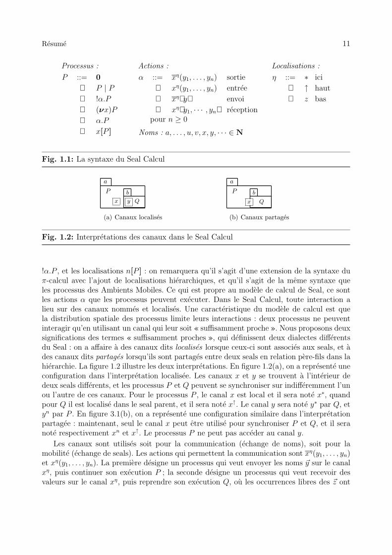
!α.P , et les localisations n[P ] : on remarquera qu’il s’agit d’une extension de la syntaxe duπ-calcul avec l’ajout de localisations hierarchiques, et qu’il s’agit de la meme syntaxe queles processus des Ambients Mobiles. Ce qui est propre au modele de calcul de Seal, ce sontles actions α que les processus peuvent executer. Dans le Seal Calcul, toute interaction alieu sur des canaux nommes et localises. Une caracteristique du modele de calcul est quela distribution spatiale des processus limite leurs interactions : deux processus ne peuventinteragir qu’en utilisant un canal qui leur soit « suffisamment proche ». Nous proposons deuxsignifications des termes « suffisamment proches », qui definissent deux dialectes differentsdu Seal : on a affaire a des canaux dits localises lorsque ceux-ci sont associes aux seals, et ades canaux dits partages lorsqu’ils sont partages entre deux seals en relation pere-fils dans lahierarchie. La figure 1.2 illustre les deux interpretations. En figure 1.2(a), on a represente uneconfiguration dans l’interpretation localisee. Les canaux x et y se trouvent a l’interieur dedeux seals differents, et les processus P et Q peuvent se synchroniser sur indifferemment l’unou l’autre de ces canaux. Pour le processus P , le canal x est local et il sera note x∗, quandpour Q il est localise dans le seal parent, et il sera note x↑. Le canal y sera note y∗ par Q, etyn par P . En figure 3.1(b), on a represente une configuration similaire dans l’interpretationpartagee : maintenant, seul le canal x peut etre utilise pour synchroniser P et Q, et il seranote respectivement xn et x↑. Le processus P ne peut pas acceder au canal y.

Les canaux sont utilises soit pour la communication (echange de noms), soit pour lamobilite (echange de seals). Les actions qui permettent la communication sont xη(y1, . . . , yn)et xη(y1, . . . , yn). La premiere designe un processus qui veut envoyer les noms ~y sur le canalxη, puis continuer son execution P ; la seconde designe un processus qui veut recevoir desvaleurs sur le canal xη, puis reprendre son execution Q, ou les occurrences libres des ~z ont

12 Resume

ete remplacees par les valeurs recues ~y. Les actions qui permettent la mobilite sont xηy etxηy1, . . . , yn. La premiere designe un processus qui veut envoyer un seal nomme y, localisedans la meme localisation que lui, sur le canal xη ; la seconde designe un processus qui veutrecevoir un seal sur le canal xη et en reactiver n copies a l’interieur des seals qu’il va creeret nommer ~zi. Il en suit que l’une des applications de la mobilite reside dans la possibilitede copier des seals, comme le montre le terme

(ν y) ( y∗x | y∗x , z ) | x[P ] qui evolue en x[P ] | y[P ] .

La semantique par reduction est definie en style chimique a l’aide d’une relation dereduction et d’une relation auxiliaire nommee congruence structurelle, qui identifie les termessyntaxiquement equivalents. La semantique par reduction est parametree sur l’interpretationdes canaux. Pour cela, nous introduisons deux predicats,

synchS, synchL : Var× Loc× Loc→ Bool

les deux abreges par synch.On suppose que la notion de noms libres d’un terme P , notee fn(P ), est connue (les lieurs

sont la restriction et le prefixe d’entree).On definit la congruence structurelle comme la plus petite relation entre processus qui

est preservee par les contextes statiques et qui verifie les axiomes suivants :

P | 0 ≡ P (νx)(νy)P ≡ (νy)(νx)P x 6= yP | Q ≡ Q | P (νx)(P | Q) ≡ P | (νx)Q x 6∈ fn(P )

P | (Q | R) ≡ (P | Q) | R (νx)0 ≡ 0!α.P ≡ α.P | !α.P

Il est interessant de remarquer que la possibilite de copier les seals invalide la regle structurelle

(νx)y[P ] ≡ y[(νx)P ] x 6= y

typique des Ambients. En effet, les processus (νx)y[P ] et y[(νx)P ] ne sont pas equivalents :si on considere un contexte C[−] = − | (ν y) ( y∗n | y∗n , m ) on obtient

C[n[(νx)P ]] _ n[(νx)P ] | m[(νx)P ] et C[(νx)n[P ]] _ (νx)(n[P ] | m[P ]) .

Le premier processus donne lieu a une configuration dans laquelle les seals n et m ont chacunun canal prive x, tandis que le second processus donne lieu a une configuration dans laquellen et m partagent un nom commun x.

La semantique par reduction est definie en style chimique. On appellera contexte statiqueun contexte de processus ou le trou ne figure pas sous un prefixe ou une duplication. Lasemantique par reduction du calcul est donc definie par la relation de reduction, _, qui estla relation la plus petite entre processus, fermee par contextes statiques et satisfaisant lesregles reportees figure 1.3.

On peut maintenant souligner un autre critere qui permet de differencier les dialectesdes Seals : la portee des noms est statique dans le Seal Calcul et, comme dans le π-calcul,la portee d’un nom peut etre etendue apres une interaction. Ce phenomene est essentiel a

Resume 13

(write local) x∗(~u).P | x∗(~v).Q _ P [~v/~u] | Q

(write in) xη1(~w).P | y[(ν~z)(xη2(~u).Q1 | Q2)] _ P | y[(ν~z)(Q1[~w/~u] | Q2)]

(write out) xη1(~u).P | y[(ν~z)(xη2(~v).Q1 | Q2)]

_ (ν~v ∩ ~z)(P [~v/~u] | y[(ν~z \ ~v)(Q1 | Q2)])

(move local) x∗~u.P1 | x∗v.P2 | v[Q] _ P1 | u1[Q] | · · · | un[Q] | P2

(move in) xη1v.P | v[S] | y[(ν~z)(xη2~u.Q1 | Q2)]

_ P | y[(ν~z)(Q1 | Q2 | u1[S] | · · · | un[S])]

(move out) xη1~u.P | y[(ν~z)(xη2v.Q1 | v[R] | Q2)]

_ P | (ν fn(R) ∩ ~z)(u1[R] | · · · | un[R] | y[(ν~z \ fn(R))(Q1 | Q2)])

(red struct) P ≡ P ′ ∧ P ′ _ Q′ ∧ Q′ ≡ Q implique P _ Q

ou x 6∈ ~z, ~w ∩ ~z = ∅, fn(S) ∩ ~z = ∅ et synchy(η1, η2).

Fig. 1.3: Regles de reduction pour le Seal Calcul

l’expressivite du calcul, mais il peut etre preferable de le limiter quand la portee d’un nomsort des limites d’une localisation a la suite d’un mouvement. On nommera cette limitationcondition-e. Ajouter la condition-e au langage revient a imposer la condition

fn(R) ∩ ~z = ∅

dans la regle de reduction (move out).

On definit comme notion basique d’observation la presence au niveau superieur d’unseal dont le nom est public : cet observable peut etre interprete comme la capacite pour uncontexte d’interagir avec ce seal. Formellement, nous ecrirons P ↓ n si et seulement si existentQ, R, ~x tels que P ≡ (ν~x)(n[Q] | R) ou n 6∈ ~x. Etant fixe cet observable, nous consideronsla congruence barbue fermee par reduction, notee ∼=, comme l’equivalence naturelle.

Les dialectes de Seal, et l’equivalence comportementale La localisation des canauxet la condition-e sont deux caracteristiques orthogonales. On peut ainsi identifier quatredialectes du Seal Calcul, definis comme suit :

– L-Seal : canaux localises ; (presque) le Seal Calcul originel presente dans [VC99] ;– eL-Seal : canaux localises et condition-e ; defini dans [CZN02] ;– S-Seal : canaux partages ; defini dans [CGZN01] ;– eS-Seal : canaux partages et condition-e ; defini dans [CZN02].

Grace a la presentation uniforme des ces calculs qu’on vient de donner, il est possible demettre en relief les differences subtiles entre ces calculs de processus apparemment similaires.

14 Resume

La surprise la plus grande a probablement ete le fait que la condition-e donne auxcontextes le pouvoir d’observer l’ensemble des noms libres d’un terme. Soient P et Q deuxprocessus, et soit x un nom tel que x ∈ fn(P ) mais x 6∈ fn(Q). Independamment du compor-tement des deux termes, le contexte

C[−] = zyn | y[(νx)(z↑n | n[− ])]

utilise le nom x pour distinguer P de Q : d’un cote, le seal n[Q] peut sortir de y, de l’autrela presence du nom libre x dans P empeche le deplacement du seal n. La condition-e donneaux contextes un grand pouvoir de discrimination et il est difficile de justifier l’equivalencequ’on obtient seulement en termes de comportement. En effet, deux processus sont considerescomme n’etant pas equivalents des lors qu’ils presentent des nom libres differents, y comprisdans des sous-processus dead-locked.

Les dialectes qui presentent des canaux localises sont caracterises par des extrusions denoms assez subtiles, comme le montre la reduction suivante :

x∗(u).P | (νz)z[x↑(v).Q] _ (νz)(P [u/v] | z[Q]) .

Ces comportements rendent le controle de l’interference tres difficile. Par exemple, les termes(νcxy)(cx | cy | x[P ]) et (νcxy)y[P ] ne sont pas equivalents : le processus P pourrait eneffet executer une action z↑(c) qui rende le nom c connu a l’environnement, qui peut ensuiteinterferer dans la reduction. Comme consequence, non seulement la theorie algebrique serevele tres pauvre, mais surtout programmer dans les dialectes localises du Seal Calcul peutconduire a des erreurs difficilement identifiables.

Le Seal Calcul avec des canaux partages et sans la condition-e se revele le calcul le pluspropice a une etude theorique : dans la suite nous nous concentrerons sur S -Seal, et onl’appellera tout simplement Seal. Nous chercherons des methodes de preuve basees sur unste, pour en apprendre plus sur son comportement et approfondir notre connaissance de satheorie algebrique.

Un systeme de transitions etiquetees En figure 1.6 nous definissons un ste pour Seal.Les transitions ont la forme

A ` P`−−→ P ′

ou A est un ensemble fini de noms tel que fn(P ) ⊆ A ; l’interpretation intuitive est « dansun etat ou les noms dans A peuvent etre connus par le processus P et son environnement, leprocessus P peut executer l’action ` et devenir P ′ ». Cette presentation, reprise depuis [SV99]et [Sew00], nous permet de simplifier les regles qui concernent l’extension de la porte desnoms. Dans les environnements des noms, on ecrit A, y pour indiquer A

.∪ {y},

Les actions `, definies figure 1.4, donnent une description precise de l’evolution d’un termeP . Les actions peuvent etre regroupees en trois classes : les actions qui sont une consequencedirecte de l’execution d’une capacite, celles qui representent une synchronisation partielle,et la reduction interne.

Un processus peut utiliser une capacite : les regles (IN), (OUT), (SND), et (RCV) ensont responsables. Les actions d’entree xη(~y) et de sortie xη(~y) sont analogues aux actionscorrespondantes dans un ste precoce de π-calcul. L’action d’envoi xηy d’un seal exprime

Resume 15

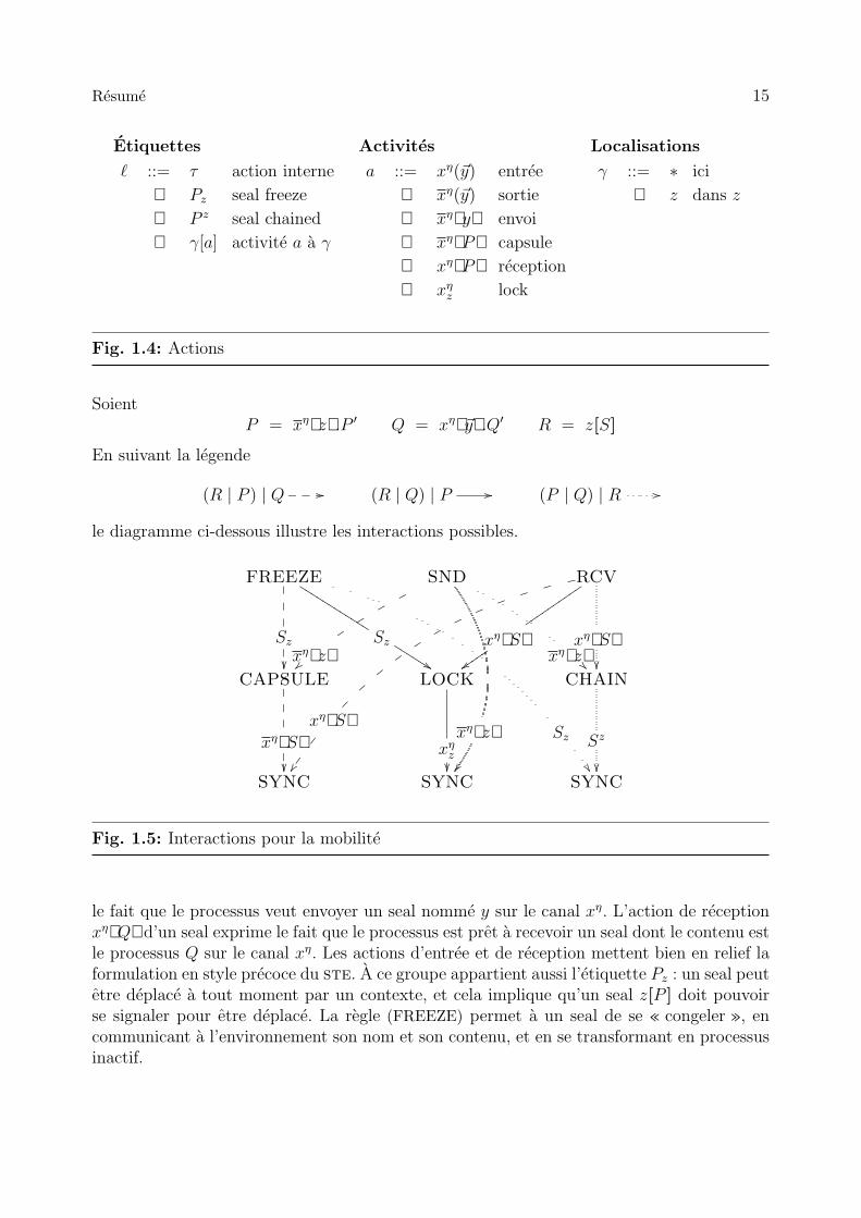
Etiquettes Activites Localisations

` ::= τ action interne

Pz seal freeze

P z seal chained

γ[a] activite a a γ

a ::= xη(~y) entree

xη(~y) sortie

xηy envoi

xηP capsule

xηP reception

xηz lock

γ ::= ∗ ici

z dans z

Fig. 1.4: Actions

SoientP = xηz.P ′ Q = xη~y.Q′ R = z[S]

En suivant la legende

(R | P ) | Q //___ (R | Q) | P // (P | Q) | R //

le diagramme ci-dessous illustre les interactions possibles.

FREEZE

Sz

���

����

Sz

��

Sz

KKKKKKKKKKKK

%%KKKKKK

SND

xηz

oq

su

}}|

xηz

xηz

��

RCV

xηS

fhik

mo

rt

wy

|�

��

�

�

xηS��

xηSuuuuuuuuuu

zzuuuuu

CAPSULE

xηS���

����

LOCK

xηz��

CHAIN

Sz

��SYNC SYNC SYNC

Fig. 1.5: Interactions pour la mobilite

le fait que le processus veut envoyer un seal nomme y sur le canal xη. L’action de receptionxηQ d’un seal exprime le fait que le processus est pret a recevoir un seal dont le contenu estle processus Q sur le canal xη. Les actions d’entree et de reception mettent bien en relief laformulation en style precoce du ste. A ce groupe appartient aussi l’etiquette Pz : un seal peutetre deplace a tout moment par un contexte, et cela implique qu’un seal z[P ] doit pouvoirse signaler pour etre deplace. La regle (FREEZE) permet a un seal de se « congeler », encommunicant a l’environnement son nom et son contenu, et en se transformant en processusinactif.

16 Resume

Le modele de mobilite du Seal Calcul demande une synchronisation entre trois processus :le processus qui deplace le seal, celui qui le recoit, et le seal qui est deplace. Comme lediagramme reporte figure 1.5 le montre, le ste peut generer les τ -actions independammentde l’ordre dans lequel elle se synchronisent. Cela demande trois etiquettes supplementaires :« capsule » xηP, « lock » xη

z , et « seal chained » P z. Ces trois etiquettes signifient que deuxdes trois intervenants dans une synchronisation ont deja interagi et attendent le troisiemeprocessus pour terminer l’interaction.

L’etiquette τ modelise les reductions internes : etant donnees deux actions en correspon-dance, la regle (SYNC) construit le processus resultant de l’interaction. Les actions corres-pondantes sont identifiees par la relation g.

Definition 3.3.1, page 72 On definit g comme la plus petite relation symetrique entreetiquettes, contenant la relation suivante :

{ (γ1[xη1(~y)] , γ2[x

η2(~y)]) | M } ∪ { (γ1[xη1S] , γ2[x

η2S]) | M }∪ { (γ1[x

η1z ] , γ2[x

η2z]) | M } ∪ { (Sz , Sz) }

ou M def= (γ1 = η1 = γ2 = η2 = ∗) ∨ (γ1 = ∗ ∧ synchγ2

(η1, η2)) ∨ (γ2 = ∗ ∧ synchγ1(η2, η1)).

Une action qui peut etre observee au niveau superieur doit etre executee ou bien au niveausuperieur, ou bien a l’interieur d’une localisation qui est elle-meme au niveau superieur. Lesetiquettes enregistrent l’endroit ou l’action a est executee avec une etiquette : ∗[a] signifieque l’action est une action executee au niveau superieur, x[a] signifie que l’action est executeea l’interieur du seal x. La regle (SEAL LABEL) transforme une etiquette ∗[a] en x[a] sous lacondition que l’action a soit observable a l’exterieur de la localisation x. Les autre regles decongruence ne necessitent pas de commentaire.

La semantique definie par le ste coıncide avec la semantique par reduction :

Theoreme 3.3.8, page 80 Soit un processus P . (i) Si fn(P ) ⊆ A et A ` Pτ−−→ Q, alors

P _ Q ; (ii) si P _ Q alors il existe A ⊇ fn(P ) tel que A ` Pτ−−→ Q′, ou Q′ ≡ Q.

Une methode de preuve Le ste qu’on vient d’introduire peut etre utilise comme baseau-dessus de laquelle definir une bisimulation etiquetee. Le developpement de cette notion debisimulation non seulement nous donnera un outil pour etudier la theorie comportementaledu Seal, mais surtout nous permettra de mieux approfondir certaines specifites de son modelede calcul.

Commencons tout d’abord par rappeler que le predicat P ↓ n teste la capacite d’unprocessus P a interagir avec l’environnement en utilisant le seal n. Dans d’autres calculs deprocessus, comme le π-calcul, les barbes sont definies en utilisant les actions du ste. Il n’estpas difficile de prouver que la relation rbc ne change pas si l’on remplace les barbes naturellespar des barbes obtenues a partir d’une certaine classe d’actions du ste (theoreme 3.4.6,page 83). Il est par contre extremement interessant d’analyser quelles actions appartiennenta cette classe, et surtout lesquelles n’y figurent pas. En effet, la classe d’actions generee parla regle (Chain) n’y figure pas, parce que les etiquettes de la forme Sz peuvent, dans certains

Resume 17

Congruence

(PAR)

A ` P`−−→ P ′

A ` P | Q`−−→ P ′ | Q

(RES) u 6∈ fn(`)

A, u ` P`−−→ P ′

A ` (νu)P`−−→ (νu)P ′

(BANG)

A ` α.P`−−→ P ′

A ` !α.P`−−→ P | !α.P

(OPEN COM) y, η, γ 6= u;u ∈ ~x

A, u ` Pγ[yη(~x)]−−−−−−−→ P ′

A ` (νu)Pγ[yη(~x)]−−−−−−−→ P ′

(OPEN FREEZE) z 6∈ u;u ∈ fn(S)

A, u ` PSz−−−→ P ′

A ` (νu)PSz−−−→ P ′

(SEAL TAU)A ` P

τ−−→ P ′

A ` x[P ]τ−−→ x[P ′]

(OPEN CAPSULE) y, η, γ 6∈ ~u;u ∈ fn(S)

A, u ` Pγ[yηS]−−−−−−−→ P ′

A ` (νu)Pγ[yηS]−−−−−−−→ P ′

(SEAL LABEL)

A ` P∗[a]−−−−→ P ′ a ∈ {y↑(~z), y↑(~z), y↑Q, y↑Q}

A ` x[P ]x[a]−−−−→ x[P ′]

Communication(OUT)

A ` xη(~y).P∗[xη(~y)]−−−−−−→ P

(IN)

A ` xη(~y).P∗[xη(~v)]−−−−−−→ P [~v/~y]

Mobilite

(SND)

A ` xηy.P∗[xηy]−−−−−−−→ P

(RCV)

A ` xη~y.P∗[xηQ]−−−−−−−→ P | y1[Q] | · · · | yn[Q]

(CAPSULE)

A ` PSz−−−→ P ′ A ` Q

∗[xηz]−−−−−−−→ Q′

A ` P | Q∗[xηS]−−−−−−−→ P ′ | Q′

(LOCK) γ = η = ∗ ou (γ 6= ∗ ∧ η =↑)

A ` PSz−−−→ P ′ A ` Q

γ[xηS]−−−−−−−→ Q′

A ` P | Qγ[xη

z ]−−−−−→ (ν fn(S) \A)(P ′ | Q′)

(FREEZE)

A ` x[P ]Px−−−→ 0

(CHAIN) γ = η1 = η2 = ∗ or (η1 = γ ∧ η2 =↑)

A ` P∗[xη1y]−−−−−−−→ P ′ A ` Q

γ[xη2S]−−−−−−−−→ Q′

A ` P | QSy

−−−→ P ′ | Q′

Synchronisation

(SYNC) `1 g `2

A ` P`1−−→ P ′ A ` Q

`2−−→ Q′

A ` P | Qτ−−→ (ν(fn(`1) ∪ fn(`2)) \A)(P ′ | Q′)

Les regles symetriques pour (PAR), (CAPSULE), (LOCK), et (CHAIN) ont ete omises.

Fig. 1.6: Un systeme de transitions etiquetees pour Seal

18 Resume

cas, ne pas etre observables. On reviendra sur ce point quand on parlera de la completudede notre bisimulation.

Une seconde remarque est qu’une barbe P ↓ n correspond a l’emission d’une etiquette

(FREEZE) par le processus en question : A ` PRn−−−→ P ′ pour un processus R arbitraire et

un ensemble de noms A ⊇ fn(P ). Par consequent, deux processus P et Q peuvent emettre lameme barbe naturelle P, Q ↓ n, meme si au niveau du ste cela correspond a deux actions a

priori differentes, comme A ` PRn−−−→ P ′ et A ` Q

Sn−−−→ Q′ ou R peut etre different de S. Lesactions generees par la regle (CAPSULE) se comportent de la meme facon. Cela est typiquedu traitement de certaines actions d’ordre superieur, qui demandent une correspondancefaible entre les processus qui sont transmis.

A bien voir, la correspondance entre les barbes naturelles et les actions (FREEZE) nousmontre que l’observation utilisee dans la rbc est insensible au processus R qui figuredans l’etiquette de l’action (FREEZE) correspondante. Une caracterisation coinductive decette equivalence doit donc ne pas demander une correspondance stricte entre les etiquettesd’ordre superieur. Nous reprenons l’approche de Sangiorgi dans sa definition de la bisimu-lation contextuelle pour HO π [San92, San96a], et nous demandons que deux processus quiexecutent des transitions d’ordre superieur soient equivalents par rapport a toute interactionpossible avec un contexte. Il y a quatre etiquettes d’ordre superieur, γ[xηS], Sz, Rz, etγ[xηR], qui peuvent etre classees en deux groupes selon leur comportement par rapport ades interactions avec le contexte.

Supposons que A ` Pγ[xηS]−−−−−−→ P ′, et soit Q un processus qu’on veut montrer equivalent

a P . Le processus P ′ est le residuel de l’interaction entre P et un contexte C[−] qui envoieun corps de seal S sur le canal xη. Dans le jeu de la bisimulation le processus Q doitpouvoir recevoir un corps de seal arbitraire sur le canal xη, sinon un contexte peut facilementdistinguer les deux processus. En meme temps, le processus S qui figure dans l’etiquette aete envoye par le contexte : les processus P et Q n’ont aucun controle sur le choix de S.Par consequent, il n’est pas restrictif de demander des processus syntaxiquement identiquesdans les etiquettes. L’action Sz est analogue a la precedente, parce que le processus S estpresente par l’environnement.

Supposons maintenant que A ` PRz−−−→ P ′, c’est-a-dire que le processus P offre le seal

z[R] qui pourra etre deplace et copie par l’environnement. Il est indispensable de demander

qu’il existe un processus Q′ tel que A ` QSz−−−→ Q′ pour un corps de seal S arbitraire, sinon

un contexte peut facilement distinguer P et Q. En meme temps, demander que R et S soientle meme processus est trop restrictif. En effet, le contexte ne peut pas analyser directementles processus R et S, mais il doit avant tout les reactiver pour interagir avec par la suite. Parconsequent, la bisimulation ne pose pas de conditions pour R et S, mais demande que lesresiduels obtenus apres une interaction avec un contexte qui recoit le seal soient equivalents.Le cas xηR est tout a fait similaire.

Il est donc necessaire de caracteriser tous les processus que l’on peut obtenir apres lamigration d’un seal : ce role est accompli par les contextes de reception. Un exemple permetd’illustrer comment ils ont ete definis. Soit A un ensemble de noms, et soit P un processus

Resume 19

tel que

A ` Pz[x↑R]−−−−−−→ P ′ .

Un contexte qui se synchronise avec cette action de P doit etre de la forme C ′[−] ≡ C[ − |xz~y.V ], pour un C[−] et V . La reduction qui en derive est

C ′[P ] ≡ C[ P | xz~y.V ] _ C[ (ν fn(R) \ A)(P ′ | y1[R] | · · · | yn[R]) | V ] .

Une propriete basique que nous demandons a notre bisimulation, ≈, est que des contextescomme C ′[−] ci-dessus ne puissent pas distinguer des processus equivalents. Dans l’exempleci-dessus cela se traduit par le processus C ′[Q] qui doit evoluer vers un processus equivalenta celui du residuel dans (3.3). Une facon d’imposer cette condition est de demander que Qexecute une action qui se synchronise avec xz~y.V , par exemple demander qu’existent S, Q′

tels que

A ` Qz[x↑S]−−−−−−→ Q′

et que le residuel de C ′[P ] soit equivalent au residuel de C ′[Q] :

C[ (ν fn(R) \A)(P ′ | y1[R] | · · · | yn[R]) | V ] ≈ C[ (ν fn(S) \A)(Q′ | y1[S] | · · · | yn[S]) | V ]

On peut factoriser le contexte C[[−] | V ], et verifier seulement que

(ν fn(R) \ A)(P ′ | y1[R] | · · · | yn[R]) ≈ (ν fn(S) \ A)(Q′ | y1[S] | · · · | yn[S]) .

Cette idee peut etre generalisee : on appelle le contexte

(ν fn(Y ) \ A)(X | y1[Y ] | · · · | yn[Y ])

un contexte de reception de z vers ↑ dans l’univers A, note DAz,↑[X,Y ]. Son environnement

associe est l’ensemble de noms libres obtenus apres avoir remplace les trous X et Y parrespectivement le residuel dans X, et le corps du seal envoye dans Y .

Definition 3.4.7, page 86 (Contexte de reception) Soit A un ensemble de noms, etsoient X et Y deux processus tels que fn(X) ⊆ A. Un contexte de reception DA

γ,η[X, Y ] etson contexte associe ADA

γ,η [X,Y ] sont respectivement un processus et un ensemble de nomsdefinis comme suit :

si γ, η = ∗, ∗, ou γ, η = z, ↑, alors

DAγ,η[X, Y ] = (ν fn(Y ) \ A)( X | z1[Y ] | · · · | zn[Y ] )

ou les noms ~z satisfont la condition fn(DAγ,η[X,Y ]) ⊆ A ∪ ~z.

Son environnement associe ADAγ,η [X,Y ] est A ∪ ~z ;

si γ, η = ∗, z, alors

DA∗,z[X,Y ] = (ν fn(Y ) \ A)( X | z[( z1[Y ] | · · · | zn[Y ] | U )] )

ou les noms ~z et le processus U satisfont la condition fn(DA∗,z[X, Y ]) ⊆ A ∪ ~z.

Son environnement associe ADA∗,z [X,Y ] est A ∪ ~z ;

20 Resume

si γ, η = ∗, ↑, alorsDA∗,↑[X, Y ] = z[X | U ] | z1[Y ] | · · · | zn[Y ]

ou les noms z, ~z et les processus U satisfont la condition fn(DA∗,↑[X, Y ]) ⊆ A∪ ~z ∪ {z}.

Son environnement associe ADA∗,↑[X,Y ] est A ∪ ~z ∪ {z}.

Nous ecrivons DA[X, Y ] quand nous quantifions sur tous les γ, η et ecrivons AD a la placede ADA

γ,η [X,Y ] si cela ne donne lieu a aucune ambiguıte.

Nous pouvons enfin definir une bisimulation etiquetee sur les processus du Seal.

Definition 3.4.8, page 86 (Bisimilarite) On appelle bisimilarite, notee ≈, la plus grandefamille de relations indexees par des ensembles finis de noms telles que toute ≈A est une re-lation symetrique sur {P | fn(P ) ⊆ A} et, si P ≈A Q, alors les conditions suivantes sontverifies :

1. si A ` Pτ−−→ P ′ alors il existe un Q′ tel que A ` Q⇒ Q′ et P ′ ≈A Q′ ;

2. si A ` P`−−→ P ′ et ` ∈ { γ[xη(~y)], γ[xη(~y)], ∗[xηy], γ[xηS], Sz, γ[xη

z ] }, alors il existe

un Q′ tel que A ` Q⇒ `−−→ Q′ et P ′ ≈A∪fn(`) Q′ ;

3. si A ` PRz−−−→ P ′ alors existent Q′, S tels que A ` Q ⇒ Sz−−−→ Q′ et pour tout contexte

admissible DA[−,−] on a DA[P ′, R] ≈AD DA[Q′, S];

4. si A ` Pγ[xηR]−−−−−−−→ P ′ alors existent Q′, S tels que A ` Q ⇒

γ[xηS]−−−−−−−→ Q′ et pour tout

contexte admissible DAγ,η[−,−] on a DA

γ,η[P′, R] ≈AD DA

γ,η[Q′, S];

5. pour toute substitution σ telle que dom(σ) ⊆ A et ran(σ) ⊆ A, on a Pσ ≈A Qσ ;

ou un contexte de reception DA[−,−] est admissible si les deux substitutions DA[P ′, R] etDA[Q′, S] sont bien formees (c’est-a-dire, s’il n’y a pas de phenomenes de capture de noms).

Les techniques standard, adaptees aux relations indexees, nous permettent de prouver quela relation ≈ existe, est unique, et est une equivalence (proposition 3.4.9, page 87).

Il est plus difficile de montrer que la bisimilarite est preservee par tous les operateurs ducalcul. On doit particulierement veiller a eviter des problemes avec les index : nous utilisonspour cela la notion de congruence indexee [Sew00].

Definition 3.4.10, page 87 (Congruence indexee) Soit R une famille de relations in-dexees par des ensembles finis de noms telles que toute RA soit une relation definie sur{P | fn(P ) ⊆ A}. On dit que R est une congruence indexee si toute RA est une equivalenceet si les conditions suivantes sont vraies :

P RA,~y Q x, fn(η) ⊆ A

xη(~y).P RA xη(~y).Q

P RA Q α 6= xη(y), fn(α) ⊆ A

α.P RA α.Q

P RA,~y Q x, fn(η) ⊆ A

!xη(~y).P RA !xη(~y).Q

P RA Q α 6= xη(y), fn(α) ⊆ A

!α.P RA !α.Q.

P RA Q x ∈ A

x[P ] RA x[Q]

P RA Q fn(R) ⊆ A

P | R RA Q | RR | P RA R | Q

P RA,x Q

(νx)P RA (νx)Q

Resume 21

On peut prouver par une longue induction sur les contextes que

Theoreme 3.4.14, page 91 La bisimilarite est une congruence indexee.

On peut aussi prouver que la bisimulation est preservee par des substitutions injectives

Lemme 3.4.15, page 92 Si P ≈A Q et f : A→ B est injective, alors fP ≈B fQ.

Ces deux proprietes nous permettent de conclure que la methode de preuve basee sur labisimulation est correcte.

Theoreme 3.4.16, page 93 (Soundness) La bisimilarite est correcte par rapport a lacongruence barbue : s’il existe un A tel que P ≈A Q, alors P ∼= Q.

A propos de la completude La bisimilarite ne coıncide pas avec la rbc pour plusieursraisons. Tout d’abord, il faut observer que la bisimilarite est en style « retarde » : les transi-tions faibles ne permettent pas l’execution d’actions τ apres une action visible. Cette formu-lation est requise, parce qu’un processus qui execute une action d’ordre superieur necessitela contribution d’un contexte de reception avant de continuer.

On remarquera aussi que le π-calcul est un sous-calcul du Seal Calcul, et caracterisercompletement la congruence barbue en π-calcul requiert un operateur explicite pour compa-rer deux noms, au moins avec un ste analogue au notre.

C’est cependant le modele de mobilite qui souleve les probleme le plus interessant. L’unedes caracteristiques de Seal est qu’un seal ne peut pas detecter s’il est deplace par l’environ-nement ou pas. Nous pouvons ainsi construire les deux processus :

P = (νx)(x∗y | x∗y) et Q = 0 .

Soit A ⊇ fn(P ). Pour tout processus S, on a A ` PSy

−−−→ ; au contraire Q n’execute aucuneaction et on en deduit que P 6≈ Q. En meme temps, aucun contexte ne peut distinguer Pet Q : par exemple C[−] = − | y[S] n’est d’aucune aide, parce que le contexte ne peutpas determiner si le seal y a ete deplace ou non. En termes techniques, cela signifie qu’aucuncontexte peut efficacement observer une action Sz.

La theorie algebrique du Seal Calcul La bisimulation permet de prouver aisement uncertain nombre de lois algebriques, comme nous le montrons page 94 et suivantes. De plus,son developpement nous a fait remarquer plusieurs caracteristiques du modele de calcul duSeal Calcul qui etaient restees inapercues pendant longtemps.

Cependant, elle demeure insuffisante pour prouver d’autres equations, principalement acause de l’absence de techniques de preuve plus raffinees, comme les techniques de preuvedites « up-to ». L’objectif de notre etude du Seal Calcul etait de jeter des bases solides,et nous pensons l’avoir fait. En meme temps, le developpement de methodes de preuvepuissantes sera l’un des buts de notre travail dans le cadre fourni par les Ambients Mobiles.

22 Resume

Les Ambients Mobiles

Le calcul des Ambients Mobiles a ete introduit par Cardelli et Gordon il y a quelquesannees [CG00b] : son influence dans le domaine a ete tres importante, mais le developpementd’un traitement semantique approprie s’est revele (historiquement) assez difficile. En effet lesAmbients Mobiles presentent des difficultes inhabituelles, qui peuvent etre resumees commesuit :

– il est difficile pour une localisation n de controler les interferences causees par d’autreslocalisations, ou bien par le processus localise dans n meme [LS00a] ;

– le modele de mobilite est asynchrone : aucune autorisation n’est demandee pour mi-grer a l’interieur d’une localisation. Comme Sangiorgi l’a observe [San01], cela peutetre a l’origine d’un phenomene dit de stuttering : un ambient peut rentrer et sortirplusieurs fois d’une localisation sans que cela soit observable. Ainsi, une caracterisationde l’equivalence observationnelle ne doit pas observer le stuttering.

– Une des lois algebriques de AM est la loi dite du « pare-feu parfait », [CG00b] :

(νn)n[P ] = 0 n inedit pour P .

Si l’on suppose P = in k.0 il est evident qu’une bisimilarite qui veut capturer cetteloi ne doit pas observer le mouvement des localisations secretes, c’est-a-dire des loca-lisations dont le nom n’est pas connu par l’environnement.

Le but de notre etude est de resoudre ces difficultes, et de donner un traitement semantiqueau calcul des Ambients Mobiles.

Les Ambients Mobiles Nous recrivons tout d’abord la syntaxe du Calcul des Ambientssur deux niveaux, en introduisant la distinction entre processus et systemes. Nous appelleronssysteme un processus qui presente au niveau superieur seulement des ambients, qui peuventeventuellement partager entre eux des noms secrets. Cette distinction nous permet de nousconcentrer sur le mouvement des agents en evitant la complexite introduite par des capacitesqui ne sont pas exercees a l’interieur d’une localisation. La syntaxe et les regles de reductionsont reportees figure 1.7. La syntaxe des processus est standard [CG00b], avec pour seuledifference que la duplication est ici remplacee par la duplication d’un processus sous prefixe.On utilise les conventions habituelles.

La semantique par reduction est definie en style chimique. La semantique par reduction ducalcul est donc definie par la relation de reduction, _, qui est la relation la plus petite entreprocessus, fermee par les contextes statiques et satisfaisant les regles reportees figure 1.7.La semantique par reduction utilise la relation auxiliaire de congruence structurelle, ≡, quiidentifie les termes syntaxiquement equivalents et permet ainsi de rapprocher les sous-termesqui vont participer a une interaction. Sa definition est standard (voir page 100). Les systemessont des processus qui ont une structure caracteristique, et les regles de la figure 1.7 decriventaussi leur evolution. On remarque que la classe des systemes est fermee par reduction.

On definit comme notion basique d’observation la presence au niveau superieur d’unambient dont le nom est public ; formellement, nous ecrivons M ↓ n si M ≡ (νm)(n[P ] |M ′)ou n 6∈ {m}. Nous ecrivons M ⇓ n s’il existe un systeme M ′ tel que M _∗ M ′ et M ′ ↓ n. Le

Resume 23

Noms : n, h, . . . ∈ N

Systemes : Processus : Capacites :M, N ::= 0 P, Q,R ::= 0 C ::= in n entrer dans n∣∣ M1 |M2

∣∣ P1 | P2

∣∣ out n sortir de n∣∣ (νn)M∣∣ (νn)P

∣∣ open n ouvrir n∣∣ n[P ]∣∣ n[P ]∣∣ C.P∣∣ !C.P

Regles de reduction :n[in m.P | Q] | m[R] _ m[n[P | Q] | R ] open n.P | n[Q ] _ P | Q

m[n[out m.P | Q] | R ] _ n[P | Q] | m[R] P ≡ Q,Q _ R,R ≡ S implique P _ S

Fig. 1.7: Les Ambients Mobiles en deux niveaux

choix de travailler avec des systemes induit naturellement une classe de contextes, nommescontextes de systeme, et generes par la grammaire suivante :

C[−] ::= −∣∣ M | C[−]

∣∣ C[−] |M∣∣ (νn)C[−]

∣∣ n[C[−] | P ]∣∣ n[P | C[−]]

L’equivalence naturelle sur laquelle nous nous concentrerons est la congruence barbue fermeepar reduction : nous reportons sa definition ci-dessous pour eviter toute confusion. La relationcbr, notee ∼=, est la plus grande relation symetrique entre systemes telle que si M ∼= N alorsles faits suivants sont verifies :

– si M _ M ′ alors il existe un systeme N ′ tel que N _∗ N ′ et M ′ ∼= N ′ ;– M ↓ n implique Q ⇓ n ;– pour tout contexte de systeme C[−], on a C[P ] ∼= C[Q].

Un systeme de transitions etiquetees Dans les Ambients Mobiles, les prefixes C

donnent naturellement lieu a des transitions de la forme PC−−→ Q ; par exemple nous avons

in n.P1 | P2in n−−−−→ P1 | P2 .

En meme temps, les capacites elementaires induisent des actions plus complexes. Nous allonsdonc definir un ste pour les Ambients Mobiles. Le ste est defini sur les processus, memesi nos equivalences mettent en relation uniquement des systemes. Nous distinguons les pre-actions, les env-actions et les τ -actions : les premieres modelisent la possibilite pour unprocessus d’executer des capacites, et les deuxiemes modelisent l’interaction d’un systemeavec son environnement. Les τ -actions representent des reductions que les termes peuventexecuter sans necessiter une contribution de l’environnement. Seules les τ -actions et les env-actions modelisent l’evolution d’un systeme.

Les pre-actions, definies figure 1.9, donnent lieu a des transitions de la forme Pπ−−→ O, ou

les etiquettes π et les residuels O sont definis dans la figure 1.8. Un residuel sera un processus

24 Resume

Pre-actions : π ::= in n∣∣ out n

∣∣ open n∣∣ enter n

∣∣ amb n∣∣ exit n

Env-actions : σ ::= k.enter n∣∣ k.exit n

∣∣ ∗.enter n∣∣ ∗.exit n∣∣ n.enter k

∣∣ k.open n

Actions : α ::= σ ∪ τ

Concretions : K ::= (νm)〈P 〉QResiduels : O ::= P

∣∣ K

Fig. 1.8: Pre-actions, Env-actions, Actions, Concretions, et Residuels

simple si π est un prefixe du langage, ou bien une concretion de la forme (νm)〈P 〉Q si leperimetre d’un ambient est mis en cause. Dans ce cas, intuitivement, P represente la partiedu systeme qui est influencee par l’action π et Q la partie qui ne l’est pas, et m est l’ensembledes noms secrets partages par P et Q. On utilisera les conventions suivantes : si K est laconcretion (νm)〈P 〉Q, alors (νr)K est une abreviation pour (νm)〈P 〉(νr)Q si r 6∈ fn(P ),et pour (νrm)〈P 〉Q sinon. De meme, K | R est defini comme (νm)〈P 〉(Q | R), ou m est telque fn(R) ∩ {m} = ∅.

Les τ -actions, definies en figure 1.10, modelisent l’evolution autonome d’un processus.

Les env-actions, definies figure 1.11, donnet lieu a des transitions de la forme Mσ−−→ N ,

ou les etiquettes σ sont definies en figure 1.8. En pratique, les env-actions transforment lesconcretions en processus en introduisant explicitement la contribution de l’environnement ala reduction. Cette contribution est toujours un ambient qui contient un processus arbitraire :le ste ne specifie pas directement ce processus, qui est specifie seulement dans le jeu de labisimulation. Pour cela nous etendons la syntaxe de processus avec le processus special ◦,pour marquer les ambients dont le contenu doit etre specifie dans le jeu de la bisimulation.Le comportement du processus ◦ est analogue a celui du processus inactif : il est seulementun marque-page. On remarque que, a la difference des pre-actions et des τ -actions, les env-actions ne presentent pas de regles structurelles : les env-actions doivent etre executees pardes systemes qui interagissent directement avec l’environnement.

On appellera actions les env-actions etendues par l’action τ .

Proposition 4.2.1, page 102 Si T est un systeme (respectivement, un processus) et Tα−−→

T ′, alors T ′ est un systeme (respectivement, un processus) qui peut contenir le processusspecial ◦.

Pour illustrer le ste, nous expliquerons les regles induites par le prefixe in, l’immigrationdes ambients. Un exemple typique d’un ambient m qui entre dans un ambient n est le suivant :

(νm)(m[ in n.P1 | P2 ] | M) | n[Q] _ (νm)(M | n[m[P1 | P2 ] | Q]) .

L’activation du prefixe in n a l’interieur de l’ambient m donne a l’ambient m la capacited’entrer dans n : nous formalisons cela avec une nouvelle action enter n. Ainsi, la regle

Resume 25

(π Pfx)

π.Pπ−−→ P

(π Repl Pfx)

!π.Pπ−−→ P | !π.P

(π Amb)

n[P ]amb n−−−−−→ 〈P 〉0

(π Exit)

Pout n−−−−−→ P1

m[P ]exit n−−−−−→ 〈m[P1]〉0

(π Enter)

Pin n−−−−→ P1

m[P ]enter n−−−−−−→ 〈m[P1]〉0

(π Res)P

π−−→ O n 6∈ fn(π)

(νn)Pπ−−→ (νn)O

(π Par)P

π−−→ O

P | Q π−−→ O | QQ | P π−−→ Q | O

Fig. 1.9: Systeme de transitions etiquetees - Pre-actions

(τ Enter)P

enter n−−−−−−→ (νp)〈P1〉P2 Qamb n−−−−−→ (ν q)〈Q1〉Q2

(∗)

P | Q τ−−→ (νp)(ν q)(n[P1 | Q1] | P2 | Q2)

Q | P τ−−→ (ν q)(νp)(n[Q1 | P1] | Q2 | P2)

(τ Par)P

τ−−→ P ′

P | Q τ−−→ P ′ | QQ | P τ−−→ Q | P ′

(τ Exit)P

exit n−−−−−→ (νm)〈k[P1]〉P2

n[P ]τ−−→ (νm)(k[P1] | n[P2])

(τ Amb)P

τ−−→ Q

n[P ]τ−−→ n[Q]

(τ Open)P

open n−−−−−→ P1 Q

amb n−−−−−→ (νm)〈Q1〉Q2

P | Q τ−−→ P1 | (νm)(Q1 | Q2)

Q | P τ−−→ (νm)(Q1 | Q2) | P1

(τ Res)P

τ−−→ P ′

(νn)Pτ−−→ (νn)P ′

(*) On impose la condition ((fn(P1) ∪ fn(P2)) ∩ {q}) = ((fn(Q1) ∪ fn(Q2)) ∩ {p}) = ∅

Fig. 1.10: Systeme de transitions etiquetees - τ -actions

(π Enter) nous donne

m[in n.P1 | P2]enter n−−−−−−→ 〈m[P1 | P2]〉0

et, en utilisant les regles structurelles (π Res) et (π Par) on obtient

(νm)(m[in n.P1 | P2] | M)enter n−−−−−−→ (νm)〈m[P1 | P2]〉M.

Cela signifie que l’ambient m[in n.P1 | P2] a la capacite d’entrer dans un ambient nommen. Si cette capacite est utilisee, l’ambient m entrera dans n, et le systeme M sera le residuel,dans la localisation originale. Clairement, cette action peut etre executee uniquement s’il ya un ambient nomme n a cote de m. La regle (π Amb) permet de tester la presence d’unambient : on a

n[Q]amb n−−−−−→ 〈Q〉0 .

La concretion 〈Q〉0 dit que Q est dans n, et 0 est dehors. Enfin, la regle (τ Enter) permet aces deux actions complementaires d’etre executees simultanement, en executant la migration

26 Resume

(Enter)

Penter n−−−−−−→ (νm)〈k[P1]〉P2

(†)

Pk.enter n−−−−−−−→ (νm)(n[◦ | k[P1]] | P2)

(Exit)

Pexit n−−−−−→ (νm)〈k[P1]〉P2

(†)

Pk.exit n−−−−−−→ (νm)(k[P1] | n[ ◦ | P2])

(Co-Enter)

Pamb n−−−−−→ (νm)〈P1〉P2

(†)

Pn.enter k−−−−−−−→ (νm)(n[P1 | k[ ◦ ]] | P2)

(Open)

Pamb n−−−−−→ (νm)〈P1〉P 2

Pk.open n−−−−−−→ k[◦ | (νm)(P1 | P2)]

(Enter Shh)

Penter n−−−−−−→ (νm)〈k[P1]〉P2

(‡)

P∗.enter n−−−−−−−→ (νm)(n[◦ | k[P1]] | P2)

(Exit Shh)

Pexit n−−−−−→ (νm)〈k[P1]〉P2

(‡)

P∗.exit n−−−−−−→ (νm)(k[P1] | n[◦ | P2])

(†) On impose k 6∈ m. (‡) On impose k 6= n et k ∈ m

Fig. 1.11: Systeme de transitions etiquetees - Env-actions

de l’ambient a l’interieur de l’ambient n, donnant lieu a la reduction originale :

(νm)(m[ in n.P1 | P2 ] | M) | n[Q]τ−−→ (νm)(M | n[m[P1 | P2 ] | Q]) .

Les env-actions modelisent l’interaction d’un agent avec son environnement. Par exemple,etant donnee la capacite

(νm)(m[in n.P1 | P2] | M)enter n−−−−−−→ (νm)〈m[P1 | P2]〉M

l’application de la regle (Enter Shh) nous donne

(νm)(m[in n.P1 | P2] | M)∗.enter n−−−−−−−→ (νm)(n[◦ | m[P1 | P2]] |M) .

Cette transition modelise un ambient secret qui entre dans un ambient n fourni par l’envi-ronnement. Le processus contenu dans n peut etre ensuite specifie, en remplacant le marque-page. Si le nom n n’etait pas secret, alors la regle (Enter) nous aurait donne la transition

m[in n.P1 | P2] | Mm.enter n−−−−−−−−→ n[◦ | m[P1 | P2]] |M

pour modeliser un ambient public m qui entre dans un ambient n fourni par l’environnement.Les regles pour l’emigration et l’ouverture d’un ambient sont analogues. Enfin, si un

systeme offre un ambient public n au niveau superieur, alors un contexte peut interagir avecle systeme en presentant un ambient qui entre dans n. La regle (Co-Enter) capture cetteinteraction entre le systeme et l’environnement.

La semantique definie par le ste coıncide avec la semantique par reduction :

Theoreme 4.2.3, page 105 Si Pτ−−→ P ′ alors P _ P ′. Si P _ P ′ alors P

τ−−→≡ P ′.

On remarque que si M ∼= N alors (i) M ⇓ n si et seulement si N ⇓ n et (ii) M =⇒ M ′

implique que il y a un systeme N ′ tel que N =⇒ N ′ et M ′ ∼= N ′. Dans la suite on utiliseraces proprietes sans mention specifique.

Resume 27

Une caracterisation de la congruence barbue fermee par reduction Notre butest la definition d’une bisimulation etiquetee qui coıncide avec la congruence barbue. Nousnous interessons a des equivalences faibles, qui font abstraction des τ -actions : pour celanous introduisons les actions faibles. Leur definition est standard : =⇒ decrit la fermeturereflexive et transitive de

τ−−→ ;α

==⇒ decrit =⇒ α−−→ =⇒ ;α

==⇒ decrit =⇒ si α = τ etα

==⇒ sinon.Avant d’introduire la bisimulation, nous avons encore besoin de clarifier comment remplacerle marque-page ◦ par un vrai processus : l’operateur • en est responsable.

Definition 4.3.1, page 108 Soient T et Ti des systemes ou bien des processus. Alors, etantdonne un processus P , on definit :

0 • Pdef= 0 (T1 | T2) • P

def= (T1 • P ) | (T2 • P ) ◦ • P

def= P

n[R] • Pdef= n[R • P ] (νn)T • P

def= (νn)(T • P ) if n 6∈ fn(P )

!C.R • Pdef= !C.(R • P ) C.R • P

def= C.(R • P )

Nous pouvons enfin introduire notre bisimulation etiquetee entre systemes.

Definition 4.3.2, page 108 (Bisimilarite) Une relation symetrique R est une bisimula-tion si M R N implique :

- si Mα−−→M ′, α 6∈ {∗.enter n, ∗.exit n}, alors il existe un systeme N ′ tel que N

α==⇒

N ′ et pour tous les processus P on a M ′ • P R N ′ • P ;

- si M∗.enter n−−−−−−−→M ′ alors il existe un systeme N ′ tel que N | n[ ◦ ] =⇒ N ′ et pour tous

les processus P on a M ′ • P R N ′ • P ;

- si M∗.exit n−−−−−−→ M ′ alors il existe un systeme N ′ tel que n[◦ | N ] =⇒ N ′ et pour tous

les processus P on a M ′ • P R N ′ • P .Deux systemes M et N sont dit bisimilaires, notes M ≈ N , s’il existe une bisimulation Rtelle que M R N .

La bisimilarite demande une quantification universelle des processus P fournis par l’en-vironnement. Ce processus remplace le marque-page ◦ qui peut avoir ete genere par lesenv-actions. La bisimilarite est definie en style tardif : la quantification existentielle precedel’universelle. On peut definir une version en style precoce de la bisimilarite, ou la quan-tification universelle de la contribution de l’environnement P precede celle de l’existencedu systeme N ′. On peut montrer facilement que, comme dans HOπ, les versions tardive etprecoce coıncident.

Il est important de remarquer que les actions ∗.enter n et ∗.exit n requierent une cor-respondance moins stricte dans le jeu de la bisimulation : ces actions ne sont pas obser-vables, et notre approche est similaire au traitement du prefixe d’entree en π-calcul asyn-chrone [ACS98].

Nous demontrons que la bisimilarite est une relation contextuelle, ce qui permet de prou-ver que la bisimilarite est une methode de preuve correcte pour rbc.

Theoreme 4.3.7, page 122 (Soundness) La bisimilarite est contenue dans la rbc.

La difficulte principale pour prouver que la bisimilarite coıncide avec la rbc est ladefinition de contextes qui permettent d’observer les actions visibles. La definition de ces

28 Resume

Ck.enter n[−] = n[◦ | done[in k.out k.out n]] | −Ck.exit n[−] = (νa)a[in k.out k.done[out a]] | n[◦ | −]

Cn.enter k[−] = (νa)a[in n.k[out a.(◦ | (νb)b[out k.out n.done[out b]])]] | −Ck.open n[−] = k[◦ | (νa, b)(open b.open a.done[out k] | a[− | open n.b[out a]])]

ou a,b et done sont inedits.

Fig. 1.12: Contextes pour les actions visibles

−1 ⊕−2 = (νo)(o[ ] | open o.−1 | open o.−2)

SPYα〈i, j,−〉 = (i[out n] | −)⊕ (j[out n] | −)si α ∈ {k.enter n, k.exit n, k.open n, ∗.enter n, ∗.exit n}

SPYα〈i, j,−〉 = (i[out k.out n] | −)⊕ (j[out k.out n] | −) si α ∈ {n.enter k}

Fig. 1.13: Contextes et processus auxiliaires

contextes Cα[−], pour toute action visible α, est reportee figure 1.12. L’ambient nomme doneest utilise comme barbe fraıche pour signaler que l’action α a ete observee. Nous demontronsqu’il existe une etroite correspondance entre les actions visibles α et leurs contextes corres-pondants Cα[−]. Le lemme suivant montre que les contextes peuvent mimer l’execution desactions visibles.

Lemme 4.3.8, page 123 Soit M un systeme et soit α ∈ {k.enter n, k.exit n, n.enter k,

k.open n}. Pour tout processus P , si Mα−−→M ′, alors Cα[M ] • P =⇒∼= M ′ • P | done[ ].

L’inverse de ce lemme requiert des definitions techniques reportees figure 1.13. Le terme⊕ implante une forme de choix interne, et les contextes SPYα〈i, j,−〉 sont des outils quipermettent de garantir que le processus P fourni par l’environnement n’execute aucuneaction. Les processus SPYα〈i, j, P 〉 peuvent observer les reductions de P du fait que l’unedes deux barbes i et j est perdue si P execute une action.

Lemme 4.3.11, page 126 Soit M un systeme, soit α ∈ {k.enter n, k.exit n, n.enter k,k.open n}, et soient i, j des noms frais pour M . Pour tout processus P avec {i, j}∩fn(P ) = ∅,si Cα[M ] • SPYα〈i, j, P 〉 =⇒∼= O | done[ ] et O ⇓i,j, alors il existe un systeme M ′ tel que

O ∼= M ′ • SPYα〈i, j, P 〉 et Mα

==⇒M ′.

Theoreme 4.3.12, page 131 (Completude) La relation rbc est contenue dans la bisi-milarite.

Resume 29

Demonstration [Esquisse] Nous demontrons que la relation R = {(M, N) | M ∼= N}est une bisimulation. Pour cela, supposons que M R N et M

α−−→M ′. Supposons aussi queα ∈ {k.enter n, k.exit n, n.enter k, k.open n}. Nous devons trouver un systeme N ′ tel queN

α==⇒ N ′ et pour tout processus P on a M ′ • P ∼= N ′ • P .L’idee de la preuve est d’utiliser un contexte particulier qui puisse mimer l’effet de l’action

α, et qui nous permette ensuite de comparer les residuels des deux systemes. Ce contexteprend la forme

Dα〈P 〉[−] = (Cα[−] | Flip) • SPYα〈i, j, P 〉

ou Cα[−] sont les contextes definis en figure 1.12 et Flip est le systeme

(νk)k[in done.out done.(succ[out k]⊕ fail[out k])] .

Les noms succ et fail ont ete choisis de sorte qu’ils soient frais. Intuitivement, l’existence dela barbe fail montre que l’action α n’a pas encore ete executee ; au contraire, l’existence desucc avec l’absence de fail assure que l’action α a ete executee, et que cette execution a eteattestee par la presence de l’ambient nomme done.

Du moment que ∼= est contextuelle, M ∼= N implique que pour tout processus P on aDα〈P 〉[M ] ∼= Dα〈P 〉[N ]. Grace au lemme 4.3.8, et par examen des reductions du processusFlip, on observe que :

Dα〈P 〉[M ] =⇒∼= M ′ •SPYα〈i, j, P 〉 | done[ ] | Flip =⇒∼= M ′ •SPYα〈i, j, P 〉 | done[ ] | succ[ ]

ou M ′ •SPYα〈i, j, P 〉 | done[ ] | succ[ ] ⇓i,j,succ 6⇓fail. Appelons ce residuel O1. A cette reductiondoit correspondre une reduction Dα〈P 〉[N ] =⇒ O2, ou O1

∼= O2. En meme temps, lacorrespondance doit preserver les barbes de O1, parce que l’on doit avoir O2 ⇓i,j,succ 6⇓fail.

Les barbes O2 ⇓succ 6⇓fail nous indiquent que O2∼= N | done[ ] | succ[ ], pour un systeme N .

Mais O2 ⇓i,j : l’observation precedente peut alors etre combinee avec le lemme 4.3.11 pour

obtenir l’existence d’un systeme N ′ tel que N ∼= N ′ • SPYα〈i, j, P 〉 et d’une action faibleN

α==⇒ N ′.Pour conclure, il nous faut montrer que pour tout processus P on a M ′ •P ∼= N ′ •P . La

relation rbc est preservee par restriction, et cela nous permet de deriver (νdone, succ)O1∼=

(νdone, succ)O2. Mais on a (νdone)done[ ] ∼= (νsucc)succ[ ] ∼= 0, et il s’ensuit que M ′ •SPYα〈i, j, P 〉 ∼= N ′ • SPYα〈i, j, P 〉. Meme raisonnement, ∼= est preservee par restriction et(νi, j)SPYα〈i, j, P 〉 ∼= P . Par consequent, nous pouvons enfin deriver M ′ • P R N ′ • P ,pour tout processus P .

Pour completer la preuve nous devons aussi considerer les actions ∗.enter n et ∗.exit n :le fait qu’elles ne sont pas observables rend ces cas beaucoup plus simples. �

Nous pouvons ainsi conclure que la bisimilarite et la congruence barbue par reductioncoıncident.

La communication synchrone de capacites peut etre ajoutee au calcul des AmbientsMobiles. Le processus de sortie 〈E〉.P envoie le message E et continue ensuite comme P ;le processus d’entree (x).Q recoit un message, le lie a la variable x dans Q, qui est ensuiteexecute. Comme discute dans [VC99, San01], la communication synchrone est raisonnabledans le modele de calcul des Ambient Mobiles, parce que la communication est toujours

30 Resume

locale. Notre ste peut etre facilement etendu pour gerer la communication, et la preuve dutheoreme 4.2.3 peut etre aisement completee. De plus, dans notre cadre la communicationne peut pas etre observee au niveau superieur : cela implique que la bisimulation peut etreappliquee au calcul etendu et que tous nos resultats restent vrais.

Techniques de preuve dites « up-to » Nous adaptons des techniques de preuve dites« up-to » a notre cadre : ces techniques permettent de reduire grandement la taille de larelation qu’il faut construire pour prouver que deux processus sont bisimilaires.

Definition (Bisimulation up-to contexte et up-to ≡) Une relation symetrique R estune bisimulation up-to contexte et up-to ≡ si P R Q implique :

- si Mα−−→ M ′′, α 6∈ {∗.enter n, ∗.exit n}, alors il existe un systeme N ′′ tel que

Nα

==⇒ N ′′, et pour tout processus P il existe un contexte de systeme C[−] et dessystemes M ′ et N ′ tels que M ′′ • P ≡ C[M ′], N ′′ • P ≡ C[N ′], et M ′ R N ′ ;

- si M∗.enter n−−−−−−−→ M ′′ alors il existe un systeme N ′′ tel que N | n[ ◦ ] =⇒ N ′′, et pour

tout processus P il existe un contexte de systeme C[−] et des systemes M ′ et N ′ telsque M ′′ • P ≡ C[M ′], N ′′ • P ≡ C[N ′], et M ′ R N ′ ;

- si M∗.exit n−−−−−−→M ′′ alors il existe un systeme N ′′ tel que n[◦ | N ] =⇒ N ′′, et pour tout

processus P il existe un contexte de systeme C[−] et des systemes M ′ et N ′ tels queM ′′ • P ≡ C[M ′], N ′′ • P ≡ C[N ′], et M ′ R N ′.

La technique de preuve up-to contexte et up-to congruence structurelle est une techniquede preuve correcte :

Theoreme Si R est une bisimulation up-to contexte et up-to ≡, alors R ⊆≈.

Nous introduisons aussi la relation d’expansion (definition 4.4.1, page 134), qui est essen-tiellement une variante asymetrique de la bisimulation permettant d’imposer des contraintessur les reductions internes executees par les systemes, et nous demontrons que la techniquede preuve up-to contexte et up-to expansion est aussi correcte (theoreme 4.4.7, page 135).

Theorie algebrique Pour montrer la puissance de nos methodes de preuve nous reportonsici deux exemples : le premier est la preuve de l’equation dite du « pare-feu parfait », lesecond montrera comment notre bisimulation est insensible au stuttering.

Theoreme 4.6.1, page 139 (νn)n[P ] ∼= 0 si n 6∈ fn(P ).

Demonstration [Esquisse] Soit S la fermeture symetrique de la relation ((νn)n[Q],0) |∀Q s.t. n 6∈ fn(Q)}. La relation S est une bisimulation up-to contexte et up-to ≡. Les casles plus delicats concernent les mouvements invisibles ∗.enter k et ∗.exit k. On ne detailleici que le premier. Si

(νn)n[P ]∗.enter k−−−−−−−→ (νn)k[◦ | n[P ′]] ≡ k[◦ | (νn)n[P ′]] alors 0 | k[ ◦ ] =⇒≡ k[◦ | 0]

et les deux residuels sont encore dans S up-to contexte et up-to congruence structurelle. �

Resume 31

Dans [San01] on montre que les equivalences comportementales barbues sont insensiblesa un phenomene dit de « stuttering », cause par des processus qui peuvent repetitivemententrer et sortir d’une localisation. En utilisant un operateur de somme non-deterministe a laCCS, l’exemple suivant donne des intuitions sur les stuttering. Les systemes

M = m[in n.out n.in n.R] et N = m[in n.out n.in n.R + in n.R]

sont en effet equivalents. Pour comprendre pourquoi le terme supplementaire de N n’influencepas son comportement, on etudie la reduction :

N | n[S] _ n[S | m[R]] .

Le processus M peut repondre au cours du jeu de la bisimulation par une sequence de troisreductions :

M | n[S] _ n[S | m[out n.in n.R]] _ n[S] | m[in n.R] _ n[S | m[R]] .

Comme l’exemple le montre, la capacite in n correspond a l’execution de trois capacitesin n.out n.in n. Meme s’il peut apparaıtre que la bisimulation que nous avons definie faitcorrespondre a chaque action une seule action (eventuellement precedee et/ou suivie par desτ -transitions), elle est insensible au stuttering. Pour le montrer, nous utilisons une variantede l’exemple ci-dessus qui n’utilise pas la somme non-deterministe.

La duplication dans les deux systemes M et N ci-dessous implante une boucle ou l’ou-verture de l’ambient l alterne avec le chemin in n.out n ; un decalage d’un cycle entre lesdeux boucles semble differencier M de N mais le stuttering rend ce decalage negligeable.

Proposition 4.6.2, page 140 Les systemes M et N definis comme

M = m[(νl)(in n.l[] | !open l.out n.in n.l[])]

N = m[(νl)(in n.out n.in n.l[] | !open l.out n.in n.l[])]

sont bisimilaires.

Demonstration [Esquisse] Soit R la fermeture symetrique de la relation

{( k[O | (νl)(in n.l[] | !open l.out n.in n.l[])] ,

k[O | (νl)(in n.out n.in n.l[] | !open l.out n.in n.l[])] )

| k et O sont arbitraires} ∪ I

ou I est la relation identique entre systemes. La relation R est une bisimulation up-tocontexte et up-to congruence structurelle. Nous detaillons le cas le plus interessant, qui de-mande qu’a l’exercice d’une capacite corresponde une sequence de trois capacites. Supposonsque M R N , avec

M = k[O | (νl)(in n.l[] | !open l.out n.in n.l[])]

etN = k[O | (νl)(in n.out n.in n.l[] | !open l.out n.in n.l[])] .

32 Resume

Supposons aussi que

Mk.enter n−−−−−−−→ n[◦ | k[O | (νl)(l[] | !open l.out n.in n.l[])]] .

Alors N peut realiser la sequence de transitions suivante :

Nk.enter n−−−−−−−→ n[◦ | k[O | (νl)(out n.in n.l[] | !open l.out n.in n.l[])]]τ−−→ n[ ◦ ] | k[O | (νl)(in n.l[] | !open l.out n.in n.l[])]τ−−→ n[◦ | k[O | (νl)(l[] | !open l.out n.in n.l[])]] .

Nous pouvons factoriser le contexte n[◦ | −] : en travaillant up-to contexte, on voit que lesresiduels sont toujours dans R. �

Cette preuve montre clairement comment l’execution des trois capacites in n.out n.in nrequise pour repondre a la capacite in n donne lieu a une action k.enter n suivie pardeux τ transitions. Les τ -transitions sont ensuite absorbees parce que la bisimilarite est uneequivalence faible.

Nous avons ainsi developpe un cadre semantique approprie pour les Ambients Mobiles deCardelli et Gordon, grace a des idees innovatrices qui permettent de modeliser la mobiliteasynchrone et le stuttering. Le cadre est complete par des techniques de preuve puissantes.Ces resultats permettent enfin de considerer les Ambients Mobiles comme un veritable calculde processus.

Une theorie des domaines pour la concurrence

Le point de depart de notre etude du Seal Calcul et des Ambients Mobiles etait leurstheories operationnelles, et l’objectif etait le developpement de leur theories semantiques.Independamment des resultats obtenus, l’approche essentiellement operationnelle suivie seprete mal a faire ressortir les relations entre les langages, et, en general, le dessin sous-jacentles systemes concurrents. C’est pour cela que dans la deuxieme partie de cette these nousdedions nos efforts a un langage enracine dans une theorie des domaines de la concurrencebasee sur les chemins d’executions.

Notre investigation entre dans une direction de recherche initiee et etudiee principalementpar Glynn Winskel et ses co-auteurs. Initialement, la theorie des categories a ete utilisee pourmettre en relation les modeles classiques de la concurrence : cela a permis non seulement decomprendre les similitudes et differences existantes parmi les constructions utilises en concur-rence, mais a aussi permis de decouvrir une notion de bisimulation, nommee bisimulation desapplications ouvertes, qui peut etre appliquee uniformement a plusieurs modeles, meme s’ilssont tres differents. Une classe de categories se prete naturellement a l’utilisation de cettebisimulation abstraite et s’est revelee une base interessante pour developper une theorie desdomaines pour la concurrence : Cattani et Winskel se sont ainsi interesses a l’etude d’une2-categorie basee sur les pre-faisceaux [CW03]. Il faut en meme temps admettre que lesconnaissances de theorie des categories requises ne sont pas triviales. La necessite d’avoir unsysteme formel pour mieux etudier ces modeles a mene Winskel et Nygaard a la definition

Resume 33

d’un langage, nomme HOPLA (acronyme pour higher-order process language), pour l’unedes categories etudiees. Ce langage s’est revele simple et expressif, et surtout adapte a l’etudede nombreux calculs de processus d’ordre superieur.

Le langage HOPLA ne prevoit pas d’operateurs pour modeliser la generation de noms,et, sous cet aspect, il est incomplet parce qu’il ne permet pas d’etudier les phenomenesspecifiques aux langages de processus modernes. Notre contribution a ete d’etendre le lan-gage HOPLA par des operateurs pour manipuler la generation de noms, sans toutefois ledenaturer. Meme si nous nous concentrerons sur ses aspects operationnels, nous commenconspar donner un apercu du modele denotationnel qui nous a guide dans sa definition.

Une theorie des domaines basee sur les chemins d’execution Les processus peuventexecuter des chemins d’execution qui sont souvent extremement compliques : cette simpleobservation suggere de construire une theorie des domaines pour la concurrence directementsur la notion de chemin, et de representer les processus comme des collections de leur cheminsd’execution.

Les chemins sont les elements des preordres P, Q, . . . nommes ordres de chemins. Lesordres de chemins jouent le role des types de processus, en decrivant la forme des cheminsque les processus peuvent realiser. La relation d’ordre permet de determiner pour un chemindonne tous ses sous-chemins. Un processus de type P est alors represente comme un sous-ensemble ferme vers le bas X ⊆ P, nomme un ensemble de chemins. Les ensembles de cheminsordonnes par inclusion sont les elements de l’ensemble partiellement ordonne P, auquel onpensera comme a un domaine pour interpreter les processus de type P. L’ordre partiel P aplusieurs proprietes interessantes :

– il est un treillis complet avec bornes superieures donnees par l’union ensembliste : ensuivant Hennessy et Plotkin [HP79], P est un domaine non-deterministe, ou les bornessuperieures sont utilisees pour interpreter la somme non-deterministe des processus ;

– tout X ∈ P est le sup de certains elements premiers : les premiers ont la forme yPp ={p′ | p′ ≤P p} et representent un processus qui peut realiser le chemin d’execution p ;

– on peut caracteriser abstraitement P comme la sup-completion de P.Cette derniere propriete attire notre attention sur les fonctions P→ Q preservant les bornessuperieures. On ecrira Lin pour la categorie qui a les ordres de chemins P, Q, . . . pour objets,et les fonctions preservant les bornes superieures P→ Q pour fleches. La categorie Lin peutetre vue comme un modele de la logique lineaire classique : l’involution P⊥ est donnee parPop, le tenseur P⊗Q par le produit des preordres P×Q, le produit P&Q et le coproduit sonttous les deux donnes par la somme disjointe des preordres P + Q, et l’espace des fonctionsP( Q est donne par Pop×Q (voir page 150 et suivantes). En meme temps, Lin ne supportepas toutes les operations associees aux langages de processus : en effet, toutes les flechespreservent les bornes superieures et, a la difference de l’operateur de prefixe, envoient lasomme vide (le processus inactif) vers elle-meme.

En suivant la discipline de la logique lineaire, on peut obtenir des fleches non-lineaires apartir de fonctions lineaires dont le domaine est sous un exponentiel. Un choix possible dansLin est de definir les exponentiels P l’ensemble des ensembles finis de chemins, ordonne par

P �P P ′ ⇔ ∀p ∈ P.∃p′ ∈ P ′.p ≤P p′ .

34 Resume

On peut alors observer qu’une fleche lineaire !P → Q correspond a une fonction Scott-continue P→ Q (page 151). Les fleches continues permettent a plusieurs operations (parmilesquelles le prefixe) d’etre interpretees : un element de P ∈ !P contient plusieurs cheminsde calcul de P et il peut etre considere comme decrivant l’execution de plusieurs copies d’unprocessus de type P.

Les fonctions continues peuvent etre utilisees pour definir une categorie qui soit un modelecompletement adequat de HOPLA [NW03]. Pour gerer la generation de noms, nous devonsfaire un pas de plus. En suivant [Sta96], on peut faire deux observations importantes quipermettent de caracteriser le modele recherche.

1. Le comportement d’un processus depend seulement d’un ensemble fini de noms, sonsupport. Pour tout ensemble de noms s on aura donc un modele P(s) pour interpreterle comportement des processus de type P qui utilisent uniquement des noms dans s.

2. Le comportement d’un processus est preserve par le renommage injectif de ses noms.Cela implique l’existence pour tout type P et pour toute injection i : s →inj s′ d’une« traduction » P(i) : P(s)→ P(s′) qui mette en relation l’espace d’interpretation P(s′)avec celui de P(s).

Un cadre adapte pour formaliser cette famille uniforme d’interpretations est fourni par lescategories de foncteurs. On ecrira I pour la categorie des ensembles finis et fonctions injec-tives, et on definit LinI comme la categorie de foncteurs et transformations naturelles entreI et Lin. On continuera a noter les objets de LinI par P, Q, ...

Une large partie de la structure de Lin peut etre etendue a LinI . Notamment le tenseur⊗,le produit &, la somme +, et l’exponentiel ! s’etendent point-a-point. D’autres constructionssont propres a LinI . La construction objet de noms permet de voir un ensemble de nomscomme un objet de Lin : son action sur s est de renvoyer l’ensemble s vu comme un ordreplat.

L’union disjointe des ensembles dans I genere une structure monoıdale symetrique surLinI [Day70]. On notera � (prononcer tenseur bizarre) le tenseur associe. L’idee derriere cetobjet est que dans un objet P � Q les deux composantes P et Q doivent avoir des supportsdisjoints. Pour illustrer cela on peut comparer les deux objets N⊗ N et N� N :

N⊗ N(s) = {(n1, n2) | n1, n2 ∈ s} N� N(s) = {(n1, n2) | n1, n2 ∈ s et n1 6= n2} .

On peut construire plusieurs espaces de fonctions dans LinI . Notre attention sera dirigeevers N ( P et !P ( Q, ou ( est l’espace de fonctions associe a ⊗. L’espace de fonctionsassocie avec �, si on restreint son domaine aux objets de noms, genere le foncteur δ : LinI →LinI , nomme foncteur de decalage. Notations : si s est un ensemble fini, nous notons s + 1l’ensemble generique obtenu en ajoutant un nouvel element, note ∗s, a l’ensemble s. Etantdonnee f : s→ s′, nous notons f + 1 : s + 1→ s′ + 1 la fonction qui se comporte comme fsur les elements de s, et qui envoie ∗s dans ∗s′ . Le foncteur de decalage est alors defini surles objets comme δP(s) = P(s + 1), et sur les fleches comme δP(i) = P(i + 1). Intuitivement,il etend l’ensemble des noms publics s par un nom inedit : dans cette optique, δ representedes fonctions qui accepterons uniquement un nom inedit en entree.

Les constructions dans LinI que nous venons de decrire permettent d’interpreter les typesdu langage new-HOPLA : nous allons maintenant etudier leur interpretation operationnelle.

Resume 35

Le langage new-HOPLA

Le langage new-HOPLA peut etre decrit comme une extension du λ-calcul simplementtype, avec un operateur de prefixe, une somme non-deterministe et des operateurs pourmanipuler des noms generes dynamiquement. Le langage est type, et le type d’un termedecrit la forme des chemins d’execution que le terme peut realiser. En suivant la structurede LinI , on obtient :

– le type de noms est designe par N ;– les types de processus sont definis par la grammaire :

P ::= 0∣∣ N⊗ P

∣∣ !P∣∣ δP

∣∣ N→ P∣∣ P→ Q

∣∣Σi∈IPi

∣∣ µj~P .(P1, . . . , Pk)

∣∣ P .

Le type Σi∈IPi ou I est un ensemble fini sera souvent note i1:P + · · ·+ ik:P. On remarque lapresence de types recursifs : les equations recursives pour les ordres de chemins peuvent etreresolues en utilisant les systemes de l’information [Sco82, LW84].

On supposera l’existence d’un ensemble infini, denombrable, de noms constants, designespar a, b, . . . et d’un ensemble infini, denombrable, de variables de noms, designees par α, β, . . ..Les noms, constants ou variables, sont designes par m, n, . . ..

m, n, . . . ::= a, b, . . . noms constants∣∣ α, β, . . . variables de noms

On supposera aussi l’existence d’un ensemble infini, denombrable, de variables de processus,designees par x, y, . . ..

Les termes sont definis par la grammaire suivante :

t, u, v ::= 0∣∣ !t processus inactif et action anonyme∣∣ n · t∣∣ πnt tenseur et projection∣∣ λx.t∣∣ tu abstraction de processus et application∣∣ λα.t∣∣ tn abstraction de nom et application∣∣ newα.t∣∣ t[n] abstraction de nom inedit et application∣∣ recx.t∣∣ x definition recursive et variable de processus∣∣ i:t∣∣ πit injection et projection∣∣ Σi∈Iti somme∣∣ Σα∈Nt somme sur les noms∣∣ [t > p(x)⇒ u] filtrage

Le support d’un terme, note n(t), est defini comme l’ensemble de ses nom constants.Le comportement des termes t du langage est decrit par la relation de transition reportee

figure 1.14. Celle-ci utilise les transitions de forme s ` tp−−→ t′, ou s est un ensemble fini de

noms constants tels que fn(t) ⊆ s et p est une action (ou motif de chemin). L’ensemble srepresente l’ensemble des noms connus dans l’univers ou evolue t. La relation ci-dessus seradonc lue ainsi : « dans un etat tel que les noms en s sont susceptibles d’etre connus par leterme t et par son environnement, le terme t peut realiser l’action p et devenir t′ ».

36 Resume

!P; s ` !t!x (x)−−−−−→ t

P; s ` tp−−→ t′ a ∈ s

N⊗ P; s ` a · t a·p−−−→ t′

N⊗ P; s ` ta·p−−−→ t′

P; s ` πatp−−→ t′

P; s ` tip (x)−−−−→ t′

P; s ` Σi∈Itip (x)−−−−→ t′

P; s ` t[a/α]p (x)−−−−→ u a ∈ s

P; s ` Σα∈Ntp (x)−−−−→ u

P; s ` t[recy.t/y]p (x)−−−−→ u

P; s ` recy.tp (x)−−−−→ u

Pi; s ` tp (x)−−−−→ t′

Σi∈IPi; s ` i:ti:p (x)−−−−−→ t′

Σi∈IPi; s ` ti:p (x)−−−−−→ t′

Pi; s ` πitp (x)−−−−→ t′

Q; s ` t[u/x]p (x)−−−−→ v s ` u : P

P→ Q; s ` λx.tu 7→p (x)−−−−−−−→ v

P→ Q; s ` tu 7→p (x)−−−−−−−→ v

Q; s ` tup (x)−−−−→ v

P; s ` t[a/α]p (x)−−−−→ v a ∈ s

N→ P; s ` λα.ta 7→p (x)−−−−−−−→ v

N→ P; s ` ta 7→p (x)−−−−−−−→ v

P; s ` tap (x)−−−−→ v

P; s.∪ {a} ` t[a/α]

p[a/α] (x)−−−−−−−−→ u[a/α]

δP; s ` newα.tnewα.p[x′[α]/x] (x′)−−−−−−−−−−−−−−→ newα.u

δP; s ` tnewα.p[x′[α]/x] (x′)−−−−−−−−−−−−−−→ u

P; s.∪ {a} ` t[a]

p[a/α] (x)−−−−−−−−→ u[a]

P; s ` tp (x)−−−−→ t′ Q; s ` u[t′/x]

q (x′)−−−−−→ v

Q; s ` [t > p(x)⇒ u]q (x′)−−−−−→ v

Dans la regle pour l’abstraction d’un nom inedit, les conditions a 6∈ n(p) et a 6∈ n(u) doiventetre verifiees.

Fig. 1.14: new-HOPLA : systeme de transitions

Les actions (ou motif de chemin) sont definies par la grammaire :

p, q, r ::= x∣∣ !p

∣∣ n · p∣∣ i:p

∣∣ newα.p∣∣ n 7→ p

∣∣ u 7→ p∣∣ p[n] .

Comme on le verra quand on parlera du typage de new-HOPLA, les actions bien typeespresentent uniquement une action anonyme !, suivie par une variable de reprise : si un termerealise une action, alors la variable de reprise enregistre la continuation du terme, et le typed’une action met en relation le type d’un terme avec les types de ses continuations.

On peut maintenant illustrer l’interpretation operationnelle des types et des termes quiles habitent.

Le type vide, 0, represente l’ensemble vide de chemins d’execution : l’unique terme de cetype est le terme inactif, 0, terme qui n’execute aucune action.

Resume 37

Le type prefixe, !P, decrit des chemins d’execution dans lesquels une premiere actionanonyme, qu’on designera par ! (prononcer bip), est realisee avant de se reduire a un chemind’execution de forme P. Le type prefixe est associe a une operation de prefixe, qui envoie unprocessus t de type P dans le terme !t de type !P. Ainsi, le terme !t realise l’action anonyme! et devient t. L’action anonyme est l’action visible elementaire sur laquelle on construit desactions plus complexes et plus informatives.

Le type somme, construit a partir d’une famille de types (Pi)i∈I , est designe par Σi∈IPi.Il est associe d’une part aux injections, qui donnent un terme i : t de type Σi∈IPi a partird’un terme t de type Pi, et d’autre part aux projections, qui a l’oppose donnent un termeπit de type Pi a partir d’un terme t de type somme decrit ci-dessus. D’un point de vueoperationnel, si t realise une action p, alors i : t realise la meme action etiquetee par i. Laprojection πit filtre les actions p realisees par t : si p a la forme j : p′, et j = i, alors πitrealise p′. Sinon, l’action est bloquee. La semantique identifie donc les termes πi(i:t) et t, et,si i 6= j, les termes πi(j:t) et 0.

Le type tenseur N⊗P designe l’action d’etiqueter avec un nom un processus de type P. Leconstructeur donne un terme n · t de type N⊗P a partir d’un terme t de type p et d’un nomn. De meme, tous les chemins d’execution de t sont etiquetes avec n. Le destructeur, designepar πnt, verifie si une action realisee par t est etiquetee par n. Si oui, il efface l’etiquette. Sinon, il bloque l’action.

Le type de l’espace des fonctions P → Q est interprete comme !P ( Q dans LinI etest analogue a l’espace des fonctions dans le λ-calcul simplement type. Un processus λx.tde type P → Q recoit un processus u qui se comporte comme P, le lie a la variable x, et secomporte ensuite comme Q. En d’autres termes, si t[u/x] realise une action p et continuecomme t′, alors λx.t realise une action u 7→ p (qui se lit « si applique a u on realise p »),et continue comme t′. L’application de processus est notee tu, pour t : P → Q et u : P.Informellement, son comportement peut etre decrit comme tu realise p et continue comme t′

si t applique a u realise p et continue comme t′. Le type de l’espace de fonctions N→ Q estinterprete comme N( Q dans LinI . Le comportement des termes λα.t et tα est analoguea celui que l’on vient de decrire.

Le type δP represente un espace de fonctions dont le domaine est N et le codomaine enest P, soumis a la contrainte que l’argument doit etre un nom inedit. Etant donne un termet de type P, le terme newα.t sera type comme δP : operationnellement il recoit en entree unnom inedit, le lie a α, et continue ensuite comme t. L’action correspondante est newα.p, quidoit etre interpretee comme « si applique a un nom inedit, il execute p » : l’identite du nomest sans importance, pourvu qu’il soit inedit. La regle operationnelle correspondante forcecette condition en etendant l’univers des noms connus s par un nouveau nom. Le destructeur,nomme application de nom inedit, est ecrit t[n], ou t : δP et n est un nom inedit pour t.

Le terme de filtrage [t > p(x)⇒ u] est fondamental pour l’expressivite de new-HOPLA.Ce terme filtre une action realisee par t contre le motif p (on rappelle qu’actions et motifssont representes par la meme syntaxe) : si les deux se correspondent, la continuation de t estpassee a u grace a la variable x. Par consequent, si le terme t a pour type P, alors l’action pest un chemin de type P avec une variable de reprise de type R, et u en general contient x.Ce terme joue le role de destructeur du prefixe : notamment les processus [!t > !x(x) ⇒ u]et u[t/x] sont identifies (voir page 164 pour d’autres exemples).

38 Resume

Le systeme de types Le systeme de types de new-HOPLA demande une attentionparticuliere dans la gestion de noms inedits. Par exemple, considerons le terme t = t′[α].L’application du nom α au terme t′ avec pour contrainte que α soit remplacee uniquementpar des noms inedits pour t′. Considerons aussi le contexte C[−] = λα.− : dans le termeC[t] = λα.(t′[α]) la variable α est abstraite par une lambda abstraction et pendant l’executionpeut etre remplacee par un nom arbitraire, notamment un nom qui n’est pas inedit pourt′. On rencontre le meme probleme avec les contextes de la forme C[−] = Σα∈N−. Uneautre difficulte surgit si une variable de processus x est libre dans t : un contexte commeC[−] = λx.− pourrait remplacer x par un terme u arbitraire. Mais α pourrait etre remplaceepar un nom qui figure dans le support de u, et rien ne garantit que le nom qui remplace αsoit inedit pour le terme t[u/x].

Un des roles du systeme de types est d’assurer statiquement que des variables de nomssupposees inedites ne soient jamais rempolacees par des noms deja connus. Pour imposer cesrestrictions, le contexte de typage ne contient pas seulement des hypotheses sur les typesassocies aux variables, comme α:N ou x:P, mais aussi des hypotheses de fraıcheur entre elles,comme (α, β) ou (α, x). La presence d’une contrainte (α, β) revele que les variables de nomsα et β ont ete supposees differentes et ne devront jamais etre identifiees. Une contrainte(α, x) enregistre le fait que dans tout environnement le nom qui remplace α doit etre ineditpour le terme qui remplace x.

A l’aide de ces informations auxiliaires, le systeme de types suppose qu’on peut abstraireune variable avec une lambda abstraction, ou une somme sur les noms, seulement si aucunehypothese de fraıcheur n’a ete faite sur elle.

Notations : on ecrit d\α pour l’ensemble de distinctions obtenu en effacant tous les couplesqui contiennent α de d ; l’ordre des variables dans une paire (α, β) n’est pas important.

Le systeme de types de new-HOPLA peut etre defini avec des jugements de la forme

A; Γ; d ` t : P

ou– A ≡ α1:N, . . . , αk:N : ensemble de variables de noms ;– Γ ≡ x1:P1, . . . , xk:Pk : fonction partielle entre variables de processus et types ;– d : ensemble de couples (α, x) ∈ A×Γ, et (α, β) ∈ A×A, qui enregistre les hypotheses

de fraıcheur.Les actions sont typees en suivant les memes procedes, meme si les jugements de typage

signalent explicitement la variable de reprise :

A; Γ; d; ; x:R ` p : P .

L’environnement de typage suit les memes intuitions que ci-dessus. La variable x est lavariable de reprise du motif p, et son type est R : le jugement est syntaxiquement differentpour bien marquer que la variable de reprise n’est pas une variable libre de l’action. Lesysteme de type de new-HOPLA est reporte figure 1.15 et figure 1.16.

La regle responsable de la generation des hypotheses de fraıcheur est la regle de l’ap-plication des nouveaux noms. Si un terme t a ete type dans l’environnement A; Γ; d et αest une nouvelle variable de noms (c’est-a-dire α 6∈ A), alors le terme t[α] est bien type,

Resume 39

A; Γ; d; ; x:R !x : !RA; Γ; d; ; x:R p : P

A; Γ; d; ; x:R α · p : N⊗ Pα ∈ A

α:N, A; Γ; d; ; x:R p : PA; Γ; (d \ α); ; x′:δR newα.p[x′[α]/x] : δP

A; Γ; d; ; x:R p : PA; Γ; d; ; x:R α 7→ p : P

α ∈ A

A; Γ; d ` u : Q A; Γ; d; ; x:R p : PA; Γ; d; ; x:R u 7→ p : Q→ P

A; Γ; d; ; x:R p : Pj j ∈ I

A; Γ; d; ; x:R (j:p) : Σi∈IPi

A; Γ; d; ; x:R t : Pj[µ~P .~P/~P ]

A; Γ; d; ; x:R t : µjP : ~PA; Γ; d; ; x:R p : P

A′; Γ′; d′; ; x:R p : P

A ⊆ A′

Γ ⊆ Γ′

d ⊆ d′

Fig. 1.15: new-HOPLA : regles de typage pour les actions

a la condition que la variable α soit remplacee seulement par des noms inedits pour tousles termes qui remplacent les variables qui peuvent apparaıtre dans t ; cela est obtenu enajoutant l’ensemble de distinctions {α}× (Γ∪A) a d.1 La regle pour le filtrage modifie aussil’ensemble de distinctions. D’un point de vue operationnel, l’operateur de filtrage substitueun sous-terme de t, dont les noms sont contenus dans A′, dans x. De meme, la regle detypage verifie qu’aucun nom dans A′ ne figure parmi les variables qui ont ete supposeesinedites pour x ; ensuite elle considere le terme u[t′/x], ou t′ est un sous-terme de t : unevariable de noms α ∈ A supposee differente de x dans le typage de u, doit maintenant etresupposee differente de toutes les variables libres de t′. Cela justifie l’ensemble de distinctions{{α} × (A′ ∪ Γ′) | (α, x) ∈ d}. A part cela, le systeme de typage est plutot standard et suitles grandes lignes des systemes de typage du λ-calcul simplement type.

On peut donner un apercu de l’interpretation de new-HOPLA dans LinI . Un environ-nement de typage α1:N, . . . , αn:N; x1:P1, . . . , xn:Pn; ∅ represente l’objet

Jα1:N, . . . , αn:N; x1:P1, . . . , xn:Pn; ∅ K : N⊗ · · · ⊗ N⊗ !P1 ⊗ · · · ⊗ !Pn

dans LinI . Cela montre que les denotations des environnements, etant donne un univers s,sont des tuples. Si l’ensemble des hypotheses de fraıcheur n’est pas vide, alors la denotationd’un environnement est un sous-ensemble de ces tuples, forme par les tuples qui verifient leshypotheses de fraıcheur. Alors, un jugement de typage A; Γ; d ` t : P represente une fonctionlineaire

JA; Γ; d ` t : P K : JA; Γ; d K→ P ,

et un jugement pour un motif de chemins A; Γ; d; ; x:R ` p : P represente une fonction lineaire

JA; Γ; d; ; x:R ` p : P K : JA; Γ; d K⊗ Rop → Pop .1Pour simplifier la notation, quand nous ecrivons {α}× (Γ∪A) nous negligeons implicitement toutes les

informations concernant les types de variables dans Γ.

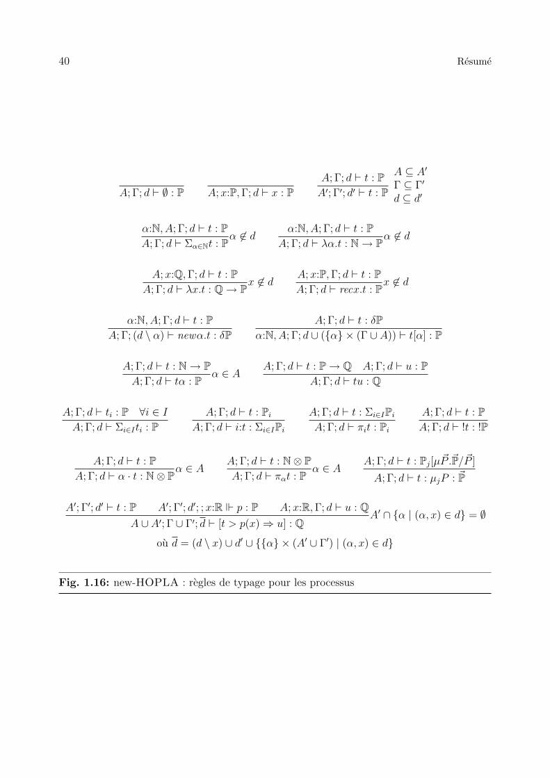
40 Resume

A; Γ; d ` ∅ : P A; x:P, Γ; d ` x : PA; Γ; d ` t : P

A′; Γ′; d′ ` t : P

A ⊆ A′

Γ ⊆ Γ′

d ⊆ d′

α:N, A; Γ; d ` t : PA; Γ; d ` Σα∈Nt : P

α 6∈ dα:N, A; Γ; d ` t : P

A; Γ; d ` λα.t : N→ Pα 6∈ d

A; x:Q, Γ; d ` t : PA; Γ; d ` λx.t : Q→ P

x 6∈ dA; x:P, Γ; d ` t : PA; Γ; d ` recx.t : P

x 6∈ d

α:N, A; Γ; d ` t : PA; Γ; (d \ α) ` newα.t : δP

A; Γ; d ` t : δPα:N, A; Γ; d ∪ ({α} × (Γ ∪ A)) ` t[α] : P

A; Γ; d ` t : N→ PA; Γ; d ` tα : P

α ∈ AA; Γ; d ` t : P→ Q A; Γ; d ` u : P

A; Γ; d ` tu : Q

A; Γ; d ` ti : P ∀i ∈ I

A; Γ; d ` Σi∈Iti : PA; Γ; d ` t : Pi

A; Γ; d ` i:t : Σi∈IPi

A; Γ; d ` t : Σi∈IPi

A; Γ; d ` πit : Pi

A; Γ; d ` t : PA; Γ; d ` !t : !P

A; Γ; d ` t : PA; Γ; d ` α · t : N⊗ P

α ∈ AA; Γ; d ` t : N⊗ PA; Γ; d ` παt : P

α ∈ AA; Γ; d ` t : Pj[µ~P .~P/~P ]

A; Γ; d ` t : µjP : ~P

A′; Γ′; d′ ` t : P A′; Γ′; d′; ; x:R p : P A; x:R, Γ; d ` u : QA ∪ A′; Γ ∪ Γ′; d ` [t > p(x)⇒ u] : Q

A′ ∩ {α | (α, x) ∈ d} = ∅

ou d = (d \ x) ∪ d′ ∪ {{α} × (A′ ∪ Γ′) | (α, x) ∈ d}

Fig. 1.16: new-HOPLA : regles de typage pour les processus

Resume 41

Le systeme de typage suppose que les termes ne contiennent pas de noms constants. Celapermet d’eviter des complications liees a un systeme de types qui gere a la fois variables denoms et noms constants. Nous ecrivons s ` t : P quand il existe un jugement A; ∅; d ` σt′ : Pet une substitution σ pour A qui respecte les hypotheses de fraıcheur d telle que t = σt′. Dememe pour les motifs.

Proposition 5.2.3, page 160 Le jugement s ` t : P est valide si et seulement s’il existeun jugement canonique A; ∅; {(α, β) | α 6= β} ` t′ : P, ou la substitution σ est une bijectionentre les variables de noms et les noms constants, et t = σt′.

Le systeme de typage verifie des proprietes attendues :

Lemme 5.2.4, page 160 (Substitution) Soient A′; Γ′; d′ ` t : Q et A; x:Q, Γ; d ` u : Pdeux jugements valides, ou Γ ∪ Γ′ est bien defini et ou A′ ∩ {α | (α, x) ∈ d} = ∅. Alors,

A ∪ A′; Γ ∪ Γ′; d ` u[t/x] : P

ou d = (d \ x) ∪ d′ ∪ {{α} × (A′ ∪ Γ′) | (α, x) ∈ d}.

Theoreme 5.2.7, page 167 (Les transitions preservent les types) Si s ` t : P et

s; ; x:Q p : P et P; s ` tp (x)−−−−→ t′, alors s ` t′ : Q.

La theorie algebrique de new-HOPLA Il est naturel d’utiliser le systeme de transitionspour definir une bisimulation : cette equivalence se revele une semantique de new-HOPLAtres interessante.

Le langage est type, et il est naturel de considerer comme equivalents uniquement lestermes qui ont le meme type. Pour cela, on dit qu’une relation R entre jugements de typagerespecte les types si chaque fois que R met en relation E1 ` t1 : P1 et E2 ` t2 : P2, on a E1 =E2 et P1 = P2. Du moment que nous sommes surtout interesses par des relations entre destermes fermes, nous ecrirons s ` t R u : P comme abreviation pour (s ` t : P, s ` q : P) ∈ R.

Definition 5.3.1, page 169 (Bisimilarite) Une relation qui respecte les types R est unebisimulation si

1. s ` t R u : P et s′ ` tp(x)−−−−→ t′ pour s′ ⊇ s impliquent qu’il existe un terme u′ tel que

s′ ` up(x)−−−−→ u′ et s′ ` t′ R u′ : R ;

2. s ` t R u : P et s′ ` up(x)−−−−→ u′ pour s′ ⊇ s impliquent qu’il existe un terme t′ tel que

s′ ` tp(x)−−−−→ t′ et s′ ` t′ R u′ : R ;

ou R est le type de la variable de reprise x dans p. On definit la bisimilarite, notee ∼, commela plus grande bisimulation.

Deux termes fermes t et q sont bisimilaires si existent s et P tels que s ` t ∼ q : P.On souligne l’importance de la quantification universelle sur tous les ensembles de noms

s′ ⊇ s. En effet, l’une des proprietes du ste est que le support d’un terme ne change pas aucours de son execution : l’existence d’univers qui contiennent d’autres noms doit donc etre

42 Resume

explicitement prise en compte dans la bisimulation, sinon la relation resultante considereraitcomme equivalents les termes

{a} ` λα.[α!0 > a!x⇒ !0] : N⊗ !0 et {a} ` λα.!0 : N⊗ !0

Or, les deux termes ci-dessus se comportent differemment dans un univers ou ils existentd’autres noms que a. Cette quantification est analogue a la quantification sur les mondespossibles des travaux sur les modeles de Kripke du λ-calcul.

La propriete fondamentale de la bisimilarite est qu’elle est une congruence par rapportaux contextes bien types.

Theoreme 5.3.14, page 176 La bisimilarite ∼ est une congruence.

Demonstration [Esquisse] La preuve utilise une variante de la methode de Howe [How96]adaptee par Gordon au cadre type [Gor95]. Pour cela nous introduisons une relation auxi-liaire, nommee candidat de precongruence, qui, par construction, contient l’extension ouvertede la bisimilarite et est preservee par les operateurs du langage. On prouve ensuite que le can-didat de precongruence est une simulation ; il s’ensuit que la fermeture transitive et reflexivedu candidat de precongruence est une bisimulation et la conclusion va de soi. �

La theorie algebrique de new-HOPLA est extremement riche, comme le montrent lesequations page 177 et suivantes.

Exemples Nous etudions l’expressivite de new-HOPLA, notamment nous montrons com-ment il peut etre utilise pour donner une semantique a des algebres de processus bien connues.A titre d’exemple nous detaillons ici le codage de la semantique tardive du π-calcul.

Tout d’abord nous definissons un type produit P & Q tres utile comme 1:P + 2:Q. Lesprojections sont fst(t) = π1(t) et snd(t) = π2(t), et le pairing est defini comme (t, u) =1:t + 2:u. Pour les actions (p,−) = 1:p, (−, q) = 2:q. Il est simple de verifier que s `fst(t, u) ∼ t : P, que s ` snd(t, u) ∼ u : Q, et que s ` (fst(t, u), snd(t, u)) ∼ (t, u) : P & Q,pour tout s ⊇ n(t) ∪ n(u).

En utilisant les conventions habituelles sur noms et variables, les termes de π-calcul sontdefinis par la grammaire suivante :

P ::= 0∣∣ P | P

∣∣ (να)P∣∣ nm.P

∣∣ n(α).P .

(Une description du systeme de transitions etiquetees en style tardif et la definition de labisimulation forte sont reportees page 179).

Le codage de la semantique tardive est reporte figure 1.17. Les termes du π-calcul sonttraduits en new-HOPLA par la fonction J− K definie par induction structurelle. L’operationde composition parallele || : P&P→ P (on utilise la notation infixe) implante la loi d’expan-sion tardive du π-calcul. Informellement, la restriction Res : δP→ P pousse les restrictionsvers l’interieur des processus : les cinq termes correspondent aux cinq equations ci-dessous :

(να)τ.P ∼l τ.(να)P

(να)mn.P ∼l mn.(να)P si α 6= m, n

(να)mα.P ∼l m(α).P si α 6= m

(να)m(β).P ∼l m(β).(να)P si α 6= m

(να)mβ.P ∼l mβ.(να)P si α 6= m

Resume 43

P = τ :!P + out:N⊗ N⊗ !P + bout:N⊗ !(δP) + inp:N⊗ !(N→ P)

J0 K = 0

Jαβ.P K = out:α · β · !JP KJα(β).P K = inp:α · !(λβ.JP K)J (να)P K = Res (newα.JP K)JP | Q K = JP K || JQ K

Res : δP→ PRes t = [t > newα.τ :!(x[α]))⇒ τ :!Res x]

+ Σβ∈NΣγ∈N[t > newα.out:β · γ · !(x[α])⇒ out:β · γ · !Res x]

+ Σβ∈N[t > newα.out:β · α · !(x[α])⇒ bout:β · !x]

+ Σβ∈N[t > newα.bout:β · !(x[α])⇒ bout:β · !newγ · Res (newη.x[η][γ])]

+ Σβ∈N[t > newα.inp:β · !(x[α])⇒ inp:β · !λγ.Res (newη.x[η](γ))]

|| : P&P→ Pt || u = [t > τ :!x⇒ τ :!(x || u)]

+ Σβ∈NΣγ∈N[t > out:(β · γ · !x)⇒ [u > inp:(β · !y)⇒ τ :!(x || yγ)]]

+ Σβ∈N[t > bout:(β · !x)⇒ [u > inp:(β · !y)⇒ τ :!Res (newη.(x[η] || yη))]]

+ Σβ∈NΣγ∈N[t > out:β · γ · !x⇒ out:β · γ · !(x || u)]

+ Σβ∈N[t > bout:β · !x⇒ bout:β · !newη.(x[η] || u)]

+ Σβ∈N[t > inp:β · !x⇒ inp:β · !λη.(x(η) || u)]

+ memes cas avec t et u echanges.

ou η ne figure pas dans u.

Fig. 1.17: π-calcul : codage de la semantique tardive

44 Resume

ou m(α) est une abreviation de (να)mα. La fonction Res implante aussi l’equation (να)P ∼0 si aucun des cas ci-dessus ne s’applique.

Il y a une correspondance stricte entre les actions executees par un processus de π-calculferme et les actions realisees par son codage.

Theoreme 5.4.3, page 180 Soit P un terme ferme de π-calcul. Alors, (i) Pτ−−→l P ′ im-

plique que n(P ) ` JP Kτ :!−−−→∼ JP ′ K ; (ii) n(P ) ` JP K

τ :!−−−→ t implique que Pτ−−→l P ′ et

t ∼ JP ′ K

De plus, le codage preserve et reflete la bisimulation forte.

Theoreme 5.4.4, page 182 et theoreme 5.4.5, page 185 Soient P et Q deux processusfermes de π-calcul. Alors P ∼l Q si et seulement si n(P, Q) ` JP K ∼ JQ K : P.

Nous proposons aussi des codages de la semantique precoce du π-calcul et de la semantiquetardive du π-calcul polyadique (page 187 et suivantes) : dans tous ces cas, nous conjecturonsque le codage est completement adequat par rapport a la bisimulation forte. Ensuite, nousnous concentrons sur l’ordre superieur, et nous proposons un codage des Ambients Mobiles(page 192). Le codage preserve et reflete les reductions des termes des Ambients Mobiles,mais il donne lieu a une equivalence qui est contenue dans l’equivalence contextuelle natu-relle (on parle ici d’equivalences fortes), mais qui ne coıncide pas avec elle. Determiner s’ilexiste un codage des Ambients Mobiles (comme de HOπ, ou de CCS avec communicationde processus) dans new-HOPLA, qui puisse reconcilier la bisimulation naturelle determineepar le codage avec la bisimulation contextuelle de Sangiorgi [San94], est un probleme ouvert.

Travaux futurs

En guise de conclusion de cette excursion dans les resultats de cette these, nous montronscomment cette these ouvre plusieurs directions de recherche.

Nos resultats sur les theories a la base du Seal Calcul et des Ambients Mobiles nousdonnent non seulement des fondations solides pour obtenir une meilleure comprehension deces calculs, mais aussi des outils pratiques pour prouver qu’une implantation respecte saspecification, ou qu’une machine abstraite est correcte. Une direction de recherche consistea raffiner nos techniques pour des domaines specifiques : notamment, nous croyons que descaracterisations etiquetees de la congruence barbue dans un cadre type peuvent etre obtenuespour les Ambients Mobiles en suivant les idees de [HMR03].

En meme temps, ces resultats ne presentent pas encore de cadre complet pour comprendrela semantique des calculs d’ordre superieur. La bisimulation contextuelle s’est revelee un ou-til tres robuste pour definir des bisimulations correctes pour des calculs d’ordre superieur :le prochaine etape consiste a developper des techniques pour eliminer la quantification uni-verselle sur tous les contextes avec lesquels un processus peut interagir. Nous avons montrecomment la technique de preuve up-to contexte permet de prouver des equations, aussi com-plexes soient-elles, en se revelant tres efficace. Cependant, il serait tres interessant de pouvoiretendre le ste propose ici pour les Ambients Mobiles a l’approche que Jeffrey et Rathke ontdeveloppe pour HOπ [JR03].

Resume 45

Un projet majeur consiste dans la definition d’axiomatisations des equivalences compor-tementales dans les calculs d’ordre superieur. En effet, meme si le raisonnement equationelest une technique centrale dans les calculs de processus, cette direction est encore vierge. Enutilisant les outils introduits pour les Ambients Mobiles, il semble possible de donner uneaxiomatisation complete de la cbr dans des calculs similaires aux Ambients Mobiles. Despremiers pas ont ete effectues dans cette direction [MZN03a].

La prolongation naturelle de notre recherche pour new-HOPLA consiste a definir etprouver les relations entre le langage et le modele denotationnel LinI . Nous nous atten-dons a un resultat d’adequation complete, ou une equivalence contextuelle (non la bisimu-lation) serait caracterisees en termes d’egalite d’ensembles de chemins. Mettre en relationla semantique operationnelle avec un modele denotationnel plus informatif, base sur les pre-faisceaux, semble presenter des difficultes additionnelles.

Un manque important de la theorie de new-HOPLA reside dans l’absence d’equivalencesfaibles. Le langage new-HOPLA ne presenta rien d’analogue aux reductions internes, et parconsequent on ne sait pas clairement comment introduire de equivalences plus abstraites.Fiore, Cattani et Winskel ont developpe un cadre mathematique pour les equivalences faiblesdans le contexte des modeles de pre-faisceaux [FCW99], qui pourrait se reveler un bon pointde depart.

Pour terminer, nous voudrions preciser les buts poursuivis : nos etudes des theoriesoperationnelles des langages de processus d’ordre superieur, et la definition de new-HOPLA,ont ete concues comme des etapes d’une part vers une comprehension approfondie du calculconcurrent, et d’autre part vers la construction d’une theorie des domaines de la concur-rence, a meme de modeliser l’ordre superieur et la generation de noms. Tous ces travauxtendent vers le projet, certes ambitieux, mais que nous esperons fructueux, de donner a laconcurrence des outils aussi feconds que les travux de Scott et Strachey l’ont ete pour lecalcul sequentiel.

2 Introduction

This thesis is about the semantics of concurrent computation.

Theories of sequential computation are essentially theories of computable functions: asequential program transforms a set of input values into output values, performing a sequenceof mechanizable steps. In this framework, the role of the denotational approach pioneeredby Scott and Strachey is essential: by providing a global mathematical setting, it placesprogramming languages in connection with each other; connects with mathematical worlds ofalgebra, topology, and logic; inspires type disciplines, programming constructs, and methodsof reasoning.

The functional view of computation finds perhaps the most serious limitations in theanalysis of concurrent systems. Here, concurrently active agents influence each other’s activ-ity on the fly by interacting in all sorts of different ways: the focus is on interaction, on thedata-flow, not on the input-output relation. Even if the classical Church-Turing thesis maybe seen as indicating that all general models of computation are equivalent, any translationfrom an expressive approach to concurrency to a formalism like that of Turing Machineswould miss ‘what really matters’, much in the same way an ‘isomorphism’ (as sets) betweenthe real line and the plane misses the mathematical understanding of space, e.g., the notionof neighbourhood.

In contrast to sequential computation, in concurrency there is no class of ‘computableprocesses’ with universal status, and global mathematical guidance is missing. Strategiesof research usually seize upon some single notion which seems to be pervasive, make it thefocus of a model, and then submit that model to various tests.

Among such notions, naming received a lot of attention. Using a name, or address, isinextricably confused with communication, an undoubtedly pervasive notion in concurrentsystems. Naming suggests the existence of an abstract space of linked processes, wherenames are used to represent links and processes interact by using names that they share.The structure of the system changes dynamically because links between processes are createdand discharged.

If mobility of links has a relatively developed theory, it is not the case when processesthemselves move in the abstract space of linked processes. The design space of languagesthat aim at seizing the notion of ‘mobile agents’ is indeed broad. At the same time standardtechniques used in concurrency do not lift smoothly to this framework. As a consequence,while there is a plethora of models that focus on mobility of active agents, their understandingis limited, and their theories form a rather fragmented picture.

This thesis addresses the theories underlying the mobile computation, with the aim todevelop mathematical tools to express and reason about systems. We focus on labelledbisimilarities to provide tractable proof methods to investigate — that is, to calculate —behavioural theories of mobile systems. Along a different line, we give an operational readingof a denotational model of non-deterministic processes. This leads us to a compact but

48 Introduction

expressive language, that directly encodes a rich variety of process languages. The unifyingconcept of this dissertation is behaviour, and what it means to say that two different processesbehave the same.

In the next two sections we introduce the main contributions of this thesis.

Background We assume that the reader has a good knowledge of first-order process calculilike CCS and π-calculus, and that he is familiar with standard techniques used in concur-rency. Basic notions of domain theory and category theory are required to understand themathematical structures that led to the definition of new-HOPLA.

2.1 On the semantics of process languages

The basic theory of CCS was developed around a labelled transition system and relatedbisimulation.

A labelled transition system, or LTS, is an inductively defined relation of the form

Pα−−→ Q .

Intuitively, the action α in the judgement Pα−−→ Q represents some small context P can

interact with, and Q is the residual of P after the interaction. For instance, in CCS, a labela stands for a possible interaction with the context Ca[−] = − | a.0. An LTS incorporatesdeep knowledge of the operational semantics of a calculus in its definition.

Bisimulation has been introduced in concurrency by Park and Milner [Par81]. Sincethen it imposed itself as a popular reference equivalence, mainly thanks to the powerfulproof methods associated. A relation between processes R is a bisimulation if wheneverP R Q the following hold:

• if Pα−−→ P ′ then there exists Q′ such that Q

α−−→ Q′ and P ′ R Q′;

• if Qα−−→ Q′ then there exists P ′ such that P

α−−→ P ′ and P ′ R Q′.

Two processes are equivalent if and only if there is a bisimulation relating them. Accordingly,bisimilarity, denoted ∼, is defined as the largest bisimulation.

These pleasingly simple notions do not lift smoothly to naming, and even less to higher-order. As a first example, the paper that introduced π-calculus [MPW92] defines two bisim-ulation based equivalences, the early and the late semantics. ‘Why two semantics?’ is aquestion that puzzled many researchers at that time. Early and late bisimilarity are todaywell understood. Yet, this anecdote suggests that grabbing a clear understanding of thesemantics of a new process calculus can be far from straightforward. As we will see below,features offered by modern process calculi lead to a series of difficulties that can be hard tocope.

Bisimulation and higher-order processes Higher-order complicates the definition of a‘sound’ labelled bisimilarity. To introduce higher-order process calculi in a gentle way, wefocus on a simple calculus, and we follow in Sangiorgi’s steps [San94].

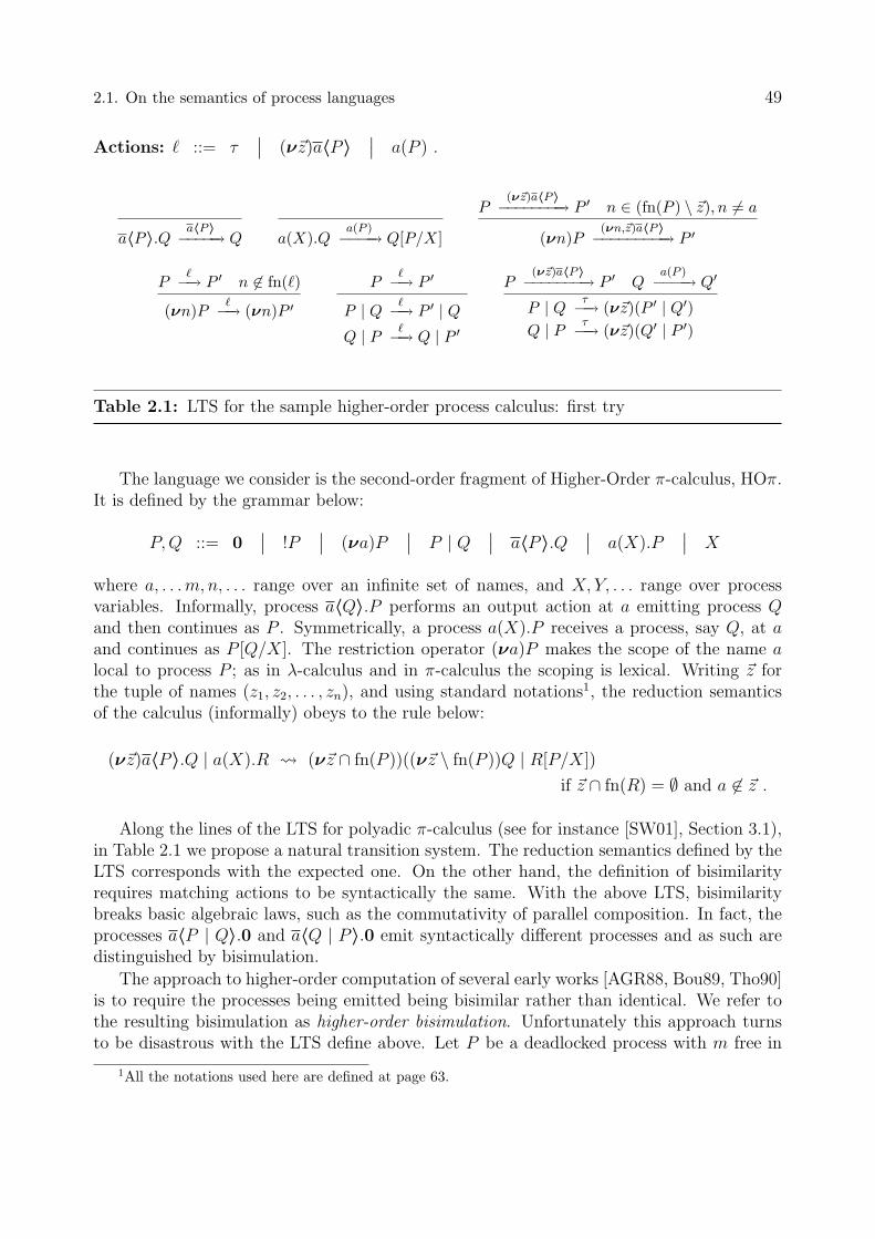
2.1. On the semantics of process languages 49

Actions: ` ::= τ∣∣ (ν~z)a〈P 〉

∣∣ a(P ) .

a〈P 〉.Qa〈P〉−−−−−→ Q a(X).Q

a(P )−−−−→ Q[P/X]

P(ν~z)a〈P〉−−−−−−−−→ P ′ n ∈ (fn(P ) \ ~z), n 6= a

(νn)P(νn,~z)a〈P〉−−−−−−−−−→ P ′

P`−−→ P ′ n 6∈ fn(`)

(νn)P`−−→ (νn)P ′

P`−−→ P ′

P | Q `−−→ P ′ | QQ | P `−−→ Q | P ′

P(ν~z)a〈P〉−−−−−−−−→ P ′ Q

a(P )−−−−→ Q′

P | Q τ−−→ (ν~z)(P ′ | Q′)Q | P τ−−→ (ν~z)(Q′ | P ′)

Table 2.1: LTS for the sample higher-order process calculus: first try

The language we consider is the second-order fragment of Higher-Order π-calculus, HOπ.It is defined by the grammar below:

P, Q ::= 0∣∣ !P

∣∣ (νa)P∣∣ P | Q

∣∣ a〈P 〉.Q∣∣ a(X).P

∣∣ X

where a, . . . m, n, . . . range over an infinite set of names, and X, Y, . . . range over processvariables. Informally, process a〈Q〉.P performs an output action at a emitting process Qand then continues as P . Symmetrically, a process a(X).P receives a process, say Q, at aand continues as P [Q/X]. The restriction operator (νa)P makes the scope of the name alocal to process P ; as in λ-calculus and in π-calculus the scoping is lexical. Writing ~z forthe tuple of names (z1, z2, . . . , zn), and using standard notations1, the reduction semanticsof the calculus (informally) obeys to the rule below:

(ν~z)a〈P 〉.Q | a(X).R (ν~z ∩ fn(P ))((ν~z \ fn(P ))Q | R[P/X])

if ~z ∩ fn(R) = ∅ and a 6∈ ~z .

Along the lines of the LTS for polyadic π-calculus (see for instance [SW01], Section 3.1),in Table 2.1 we propose a natural transition system. The reduction semantics defined by theLTS corresponds with the expected one. On the other hand, the definition of bisimilarityrequires matching actions to be syntactically the same. With the above LTS, bisimilaritybreaks basic algebraic laws, such as the commutativity of parallel composition. In fact, theprocesses a〈P | Q〉.0 and a〈Q | P 〉.0 emit syntactically different processes and as such aredistinguished by bisimulation.

The approach to higher-order computation of several early works [AGR88, Bou89, Tho90]is to require the processes being emitted being bisimilar rather than identical. We refer tothe resulting bisimulation as higher-order bisimulation. Unfortunately this approach turnsto be disastrous with the LTS define above. Let P be a deadlocked process with m free in

1All the notations used here are defined at page 63.

50 Introduction

Actions: ` ::= τ∣∣ a〈P 〉

∣∣ a(P ) .

A ` a〈P 〉.Qa〈P〉−−−−−→ Q A ` a(X).Q

a(P )−−−−→ Q[P/Q]

A,n ` Pa〈P〉−−−−−→ P ′ n ∈ fn(P ), n 6= a

A ` (νn)Pa〈P〉−−−−−→ P ′

A,n ` P`−−→ P ′ n 6∈ fn(`)

A ` (νn)P`−−→ (νn)P ′

A ` P`−−→ P ′

A ` P | Q `−−→ P ′ | Q

A ` Pa〈P〉−−−−−→ P ′ A ` Q

a(P )−−−−→ Q′

A ` P | Q τ−−→ (ν fn(P ) \A)(P ′ | Q′)

Table 2.2: LTS for the higher-order process calculus: second try

it, like (νn)n(X).m(Z).0, and Q be an arbitrary process with Y 6∈ fv(Q). Then this choiceequates the processes

(νm)(a〈m(Y ).Q〉.m〈0〉.0) and (νm)(a〈P 〉.m〈0〉.0)

which have completely different possibilities of interactions. In fact,

(νm)(a〈m(Y ).Q〉.m〈0〉.0) | a(X).Xτ−−→ (νm)(m〈0〉.0 | m(Y ).Q)

(νm)(a〈P 〉.m〈0〉.0) | a(X).Xτ−−→ (νm)(m〈0〉.0 | P )

where (νm)(m〈0〉.0 | P ) is deadlocked, while (νm)(m〈0〉.0 | m(Y ).Q)τ−−→ (νm)(0 | Q)

and Q can engage in arbitrary interactions. Also, this treatment of extruded names yieldsthe law

(νm)(a〈P 〉.Q) ∼ a〈(νm)P 〉.Q

which is difficult to justify because in the first process all copies of P activated by its recipientshare the name m, whereas in the second one, the name m is private to each copy.

The roots of these problems seem to be related to the fact that scope extrusions figurein the labels: in Table 2.2 we define an alternative LTS, extending the LTS for π-calculus

defined in [Sew00]. Transitions have the form A ` P`−−→ Q, where A is a finite set of names

such that fn(P ) ⊆ A; they should be read as “in a state where the names A may be knownby process P and by its environment, the process P can do ` to become Q”. The twoproposed LTS agree on internal reductions, and they define the same reduction semantics. Ifwe define a higher-order bisimulation on top of the LTS above2, we end up with a semanticsthat does not equate

a〈0〉.0 and (νm)a〈m〈0〉.0〉.0

as m〈0〉.0 is not bisimilar to 0. On the other hand, in any context the two processes abovegive rise to the same sequence of transitions because the process m〈0〉.0 is deadlocked as noother process knows the name m needed to ‘unlock’ it.

2A little care is required to keep the indexing straight, see Section 3.4.8.

2.1. On the semantics of process languages 51

Even if we forget about scope extrusions, higher-order bisimulation, in any of the LTSsabove, appears over-discriminating. In fact, it does not equate the processes

a〈0〉.! m〈0〉.0 and a〈m〈0〉.0〉.! m〈0〉.0 .

Yet, the replication ! m〈0〉.0 covers the difference between 0 and m〈0〉.0 regardless of howmany copies of them are used.

Barbed congruence Because of these complications, new process calculi are often pre-sented as programming languages. Technically this means to give their syntax, and specifyhow a program can be evaluated with respect to a given abstract machine. Once a clearevaluation strategy has been sketched, a notion of observation is introduced, and an equiva-lence is then derived using contextual equivalence or, if branching time is taken into account,barbed equivalence [MS92, HY95].

A good example is offered by the original paper on Mobile Ambients by Cardelli andGordon [CG00b]. They define the syntax of Mobile Ambients:

P, Q ::= 0∣∣ P | Q

∣∣ !P∣∣ (νz)P

∣∣ n[P ]∣∣ π.P

π ::= in n.P∣∣ out n.P

∣∣ open n.P

and they give its operational semantics3 as a set of reduction rules for the Chemical AbstractMachine [BB92]:

n[in m.P | Q] | m[R] _ m[n[P | Q] | R ]

m[n[out m.P | Q] | R ] _ n[P | Q] | m[R]

open n.P | n[Q ] _ P | Q

Shortly thereafter, Cardelli and Gordon introduce a Morris-style contextual equivalence (oth-erwise known as may-testing equivalence) for Mobile Ambients: two processes are contex-tually equivalent if and only if they admit the same elementary observations whenever theyare inserted inside any arbitrary enclosing process. They identify the presence of an ambientwhose name is not restricted at the top-level of a process as basic observation. This notionof observation is reminiscent of the report of the successful outcome of an experiment ina theory of testing equivalence [DH84, Hen88]. In such a theory the basis for comparingprocesses is the results of experiments in which the processes are tested by composing themwith special terms.

More in detail, a process P converges to a name n if after some reductions, P exhibitsan ambient named n. Formally,

P ↓ n = P ≡ (ν ~z) (n[P1] | P2) for some P1, P2 and set of names ~z such that n 6∈ ~z;

P ⇓ n = either P ↓ n or P _ P ′ for some P ′ and P ′ ⇓ n.

3Mobile Ambients is the object of Chapter 4: a complete description its syntax and semantics (inparticular the definition of the structural equivalence relation, ≡) can be found there.

52 Introduction

Then contextual equivalence is the relation P ∼= Q defined by:

P ' Q iff for all n and C[−], C[P ] ⇓ n⇔ C[Q] ⇓ n .

Contextual equivalence does not take into account the branching structure of processes.Branching time informations can be added to testing theories in several different ways.Barbed equivalence provides a simple method to construct a branching time equivalencerelation. The idea is to impose a bisimulation structure over reduction steps, and also askthat at each step observations are preserved. As in general barbed equivalence is far frombeing a congruence for the language, barbed congruence is commonly used.

We introduce a variant of barbed congruence, called reduction barbed congruence. Re-duction barbed congruence, denoted ∼=, is the largest symmetric relation such that wheneverP ∼= Q the following hold:

• if P _ P ′ then there exists a process Q′ such that Q _∗ Q′ and P ′ ∼= Q′;

• P ↓ n implies Q ⇓ n;

• for all contexts C[−], it holds C[P ] ∼= C[Q];

where _∗ denotes the reflexive and transitive closure of _.Observe that reduction barbed congruence, as defined above, abstracts from internal

reduction, that is, it is a weak equivalence. In a distributed setting, it is the visible actionsthat are of most interest.

The definition of barbed congruence is simple and robust. Yet, it involves quantificationover all contexts, making it harder to prove instances of the equivalence (even if Fournet’sthesis [Fou98] presents useful techniques). Also, as all ready-made recipes, its definition doesnot provide in a direct way any information on the behavioural theory of the calculus.

The need for labelled bisimilarities Let us go back to Mobile Ambients. Even a notionof equivalence as simple as contextual equivalence suffices to point out some peculiarities ofits behavioural theory. Consider a process (ν n) n[P ] where n is not free in P . Since thename n is know neither inside the ambient n[P ], nor outside it, the ambient n[P ] is a ‘perfectfirewall’ that neither allows another ambient to enter nor to exit. This is formalised by theequation below (also known as the perfect firewall equation):

(ν n) n[(ν n) P ] ∼= 0 .

This equation has been proved in [GC02] by a long induction over contexts. For quite a longtime the perfect firewall equation has been (almost) the only equation formally proved, andsummarised all what was known about Mobile Ambients semantics.

The desire to investigate more in detail the behavioural theory of Mobile Ambients,led Levi and Sangiorgi to define a dialect of Ambients, called Safe Ambients : in this novelcalculus interaction is more constrained than in Ambients. As a consequence, more equationsare valid, and in general their proofs are easier. In [MH01], Merro and Hennessy developa labelled bisimilarity that coincides with reduction barbed congruence for (a variant) of

2.1. On the semantics of process languages 53

Safe Ambients. Along a parallel line of research, for the subset of Mobile Ambients withoutname restriction, Sangiorgi [San01] shows that the equivalence induced by the spatial logicsby Cardelli and Gordon [CG00a] coincides with structural congruence. This means that theambient logic captures the intensional structure of a process, but not its behaviour.

All these attempts show how elusive can be capturing contextual equivalence or barbedcongruence with a labelled bisimilarity. They also show how many efforts are devoted tothe quest. In fact, the name calculus implies the ability to do equational reasoning, thatis, to calculate. The definition of labelled bisimilarities that imply, or better coincide with,reduction barbed congruence is fundamental tool to investigate the behavioural theory ofthe calculus. More than that, their development usually provides a great deal of insightinto the meaning of barbed congruence, and very fine grained information on equivalentprocesses [San92, ACS98, FG98].

The Seal Calculus and Mobile Ambients The first part of this dissertation is devotedto the study of the behavioural theories of two process calculi that present two orthogonalmodels of agent mobility. Both assume the existence of basic spatial objects, called loca-tions. A location abstracts either a physical place, such as hosts or networks, or a logicalentity, such as operating system processes or finer grained isolated software components likewrappers [SV99]. To play these different roles, locations are structured in a tree-like hierar-chy in which each level models some ‘real world’ entity. Mobility amounts to perform localchanges in the tree-like hierarchy of locations. Both offer ‘strong’ mobility: a process can beinterrupted during its execution and moved together with its current environment to anotherlocation where execution is pursued. In the Seal Calculus a location is displaced by processesin its environment and has no control on migration: a location is a passive component of thereduction. On the other hand, in Mobile Ambients the migration instruction comes fromthe migrating entity itself: locations are active components, and move under the controlof the processes located inside them. Under the assumptions that the ‘reference frame’ ishierarchical, and that routing of messages across distant locations must be explicitly pro-grammed, the study of these two models covers a wide range of the spectrum of possiblemobility primitives.

Contributions The name Seal Calculus has been used to denote a family of dialects thatevolved from the Seal Calculus as introduced in [VC99]. These dialects share the same designchoices and provide the programmer with the same set of abstractions, but little (and sur-prisingly subtle) differences can found in their reduction semantics. Our investigation aimsto tidy up the confused picture offered by these apparently similar dialects, as well as todevelop solid foundations for Seal. We give a uniform presentation of the syntax and of thereduction semantics of all of the dialects. A preliminary investigation of their behaviouraltheories highlights the deep differences between these process calculi, only superficially sim-ilar. We concentrate on the dialect that appears at the same time a suitable kernel for aprogramming language and a process calculus amenable of theoretical investigation. Wepropose a labelled transition system: its definition points out some of the particularitiesof the Seal model of computation. On top of the LTS we build a labelled bisimilarity and

54 Introduction

we prove that it is a sound proof technique for reduction barbed congruence. The labelledbisimilarity is subsequently used to prove some algebraic laws.

In the framework of Mobile Ambients, we devote our efforts to develop powerful bisim-ulation based proof techniques. First, as in the Distributed π-calculus [HR98], we rewritethe syntax of Mobile Ambients in two levels: processes and systems. We are interested instudying systems and movement of code, rather than processes: the two level syntax allowsus to focus on higher-order actions, avoiding the overhead caused by actions fired at top-level. We introduce a new labelled transition system for Mobile Ambients which is used todefine a labelled bisimilarity over systems. The resulting bisimilarity can be defined eitherin late or in early style. However, as in HOπ [San96a], the two formulations coincide, andwe concentrate on the easier late version, denoted ≈. The definition of ≈ reminds us theasynchronous bisimilarity found in [ACS98]. Indeed, as for inputs in asynchronous π, ourbisimilarity does not observe the movements of secret ambients. The relation ≈ completelycharacterises reduction barbed congruence over systems. Then, we enhance our proof meth-ods by defining two up-to proof techniques, along the lines of [MS92, San98, SW01]. Moreprecisely, we develop both up-to expansion and up-to context proof techniques and provetheir soundness. We are not aware of other forms of up-to proof techniques for higher-ordercalculi. Finally, we apply our bisimulation proof methods to prove a collection of both oldand new algebraic laws (including the perfect firewall equation); we also prove the correctnessof the protocol, introduced in [CG00b], for controlling access through a firewall.

2.2 A process language out of a semantic model

In the first part of the thesis bisimulation based proof methods are used as a common groundto study the intrinsic theory of two already existing process calculi. That is, we start fromtheir definitions and we develop their foundations. In the second part of the dissertation,the syntax and the operational theory of an expressive language are derived starting fromits roots in a domain theory for concurrency based on paths, that is, from its foundations.

We put aside operational semantics for a while, and we review a line of research aimingto provide a common mathematical framework to investigate the semantics of concurrency.

Bisimulation from open maps Starting from the work [WN95], Winskel and Nielsenconcentrate on understanding the structure of different models for concurrency and how theyrelate. Category theory has been the natural tool for this task. Their approach turns eachclass of models into a category, whose objects are models, and whose morphisms stand forsimulations. As an example consider the category of transition systems4 T (for brevity weassume a common set of labels A), and let T1 = (S1, i1, A, −→1), T2 = (S2, i2, A, −→2) betwo transition systems. A morphism f : T1 → T2 in T is a function f : S1 → S2 such thatf(i1) = i2 and t1 −→1 t2 implies ft1 −→2 ft2. Observe that f expresses how T1 may besimulated by T2. Synchronisations trees arise as a full subcategory of transitions systems.The familiar operation of unfolding a transition system into a synchronisation tree appears

4A transition system is a structure (S, i, A, −→) where S is a set of states, i a distinguished initial state,A a set of labels, and −→ is the transition relation, that is a subset of S ×A× S.

2.2. A process language out of a semantic model 55

as a right adjoint to the inclusion functor S→ T. Similar constructions can be carried overalso in causal models, like event structures and Petri nets. This presentation not only makesprecise how different models relate, but also exposes operations like nondeterministic sumand parallel composition found in process calculi as universal constructions.

Morphisms in a category are understood as kinds of functional simulations. A definitionof bisimulation across the categorical models can be built by identifying those morphismsthat not only preserve but also reflect behaviour. Consider again the two transitions systemsdefined above. A morphism f : T1 → T2 is said to be a zig-zag morphism (or abstraction

homomorphism [Cas85]) if whenever fsα−−→2 t′ there is a state t ∈ S1 such that s

α−−→ tand ft = t′. It is clear that if f is a zig-zag morphism then its graph is a bisimulationbetween the two transition systems. In categorical terms, suppose we are given a sequenceof transitions in T1:

p1 : i1α1−−−→ r1

α2−−−→ r2α3−−−→ . . .

αn−−−→ s1

Since f : T1 → T2 is a morphism, this induces a simulating sequence in T2:

p2 : i2α1−−−→ fr1

α2−−−→ fr2α3−−−→ . . .

αn−−−→ fs1

If f is zig-zag, then any extension q2 of p2 with an extra transition fs1α−−→ s′2, implies that

also p1 can be extended to a sequence

q1 : i1α1−−−→ r1

α2−−−→ r2α3−−−→ . . .

αn−−−→ s1α−−→ s′1 ,

where s′1 is such that fs′1 = s′2. Now, the four sequences above are themselves transitionsystems, and objects of T. Clearly p1

∼= p2 and q1∼= q2, and we will refer to them as p and

q. As q is an extension of p there is an obvious morphism e : p → q, and because p is asequence of T1 and q a sequence of T2 we have morphisms x : p→ T1 and y : q → T2, so thatthe square on the left below commutes. Commutativity rephrases the fact the simulationsby T2 of p can be extended to the simulation of q.

p

e

��

x // T1

f��

qy// T2

p

e

��

x // T1

f��

q

z@@

y// T2

The zig-zag requirement on f can then be stated by saying that any such commutativesquare can be split into two commutative diagrams as on the right above. Commutativityof the upper triangle expresses that the sequence in T1 that simulates q is an extensionof the sequence simulating p. The lower triangle amounts to saying that this extension iscompatible under f with the sequence simulating q in T2.

It is reasonable to think to objects p and q as computation paths. In the model of transitionsystems they correspond to sequences of transitions, that is, traces. In general, computationpaths may have more structure than traditional traces, e.g., allowing path semantics to takenondeterministic branching into account in a limited way.

Abstractly, let M be any category of models and be P be a subcategory P→M thoughtof as the category of the computation paths of M. We define P-open maps to be those

56 Introduction

morphisms f of M such that for all morphisms e : p → q in P, any commuting square likethat on the left can be split into two commuting triangles as on the right. We say thattwo models M and N of M are open map bisimilar if there exists a span M ← O → N ofopen maps between them. In the case of transition systems and the subcategory of finitesequences, open-map bisimilarity coincides with Park and Milner’s bisimulation. Reasonableequivalence are obtained for other models as well, see [JNW94].

Presheaf models Open map bisimulation provides an abstract way to uniformly definebisimulation on models for concurrency, once a suitable subcategory of paths has been chosen.There is much freedom in the choice of the subcategory P, whose only requirement is to bea subcategory of the model.

But an important class of categories are equipped with a canonical choice for a pathcategory: these are the so-called presheaf categories. The objects of a presheaf category,called presheaves, can be understood as the collection of processes constructed from itscanonical underlying path category by freely adding coproduct (nondeterministic sums ofpaths) and coequalisers (gluing paths together by identifying subpaths). An alternativeview is that a presheaf, seen as a process, assigns to each computation path the set of waysit is simulated by, or ‘realised by’, the process. In the light of the above, Cattani and Winskelhave drawn attention to a 2-categorical model of linear logic and associated comonads, basedon presheaves [CW03]. The categorical overhead involved is quite conspicuous.

In general it is quite inconvenient to work directly in a specific category or with a specificmonad. Mathematical logic provides a simple recipe to abstract away from specific models:fix a language, define what is an interpretation of the language in a model, find a formalsystem (on the language) that captures the desired properties of models. When the formalsystem is sound, one can forget about the models and use the formal systems instead.Moreover, if the formal system is also complete, then nothing is lost (as far as one is concernedwith properties expressible in the language, and valid in all models).

This led Nygaard and Winskel to the discovery of two expressive metalanguages forconcurrency, called HOPLA (Higher Order Process LAnguage) and AL (Affine Language).The presheaf semantics led to operational semantics, guided by the idea that derivations oftransitions in the operational semantics, associated with paths, should correspond to realisersin the presheaf definitions. Process calculi such as CCS, CCS enriched with process passing,and Mobile Ambients with public names can be encoded in HOPLA.

The language new-HOPLA Although surprisingly expressive, HOPLA cannot modelname generation, one basic ingredient of mobile systems, and, in general, of modern processcalculi. In the second part of this thesis, we study an extension to equip HOPLA with namegeneration.

At the level of the domain theory, the idea is to work in a functor category indexed bythe category of finite sets and injective functions. We give an account of the denotationalmodel using path sets, rather than presheaves. Even if path sets are considerably simplerthan presheaves, they furnish a model which is sufficiently rich in structure to show hownew-HOPLA arises from canonical constructions on path sets. For the most part new-HOPLA lends itself to an operational account. As for HOPLA, the intuitions on the

2.3. Overview 57

interpretation lead us to the development of a syntax, of a type system, and of an operationalsemantics. The language new-HOPLA can be viewed as an extension of the simply typed λ-calculus with prefixing, sums, and constructs to manipulate dynamically generated names.We investigate its operational theory. Particular attention is devoted to the bisimulationequivalence that arises naturally, and we show that it is a congruence for the language. Richprocess algebras can be faithfully encoded into new-HOPLA. We define an encoding of π-calculus that not only preserves and reflects the reduction semantics, but also the behaviouraltheory. We also provide encodings of polyadic π-calculus and of Mobile Ambients.

2.3 Overview

Outline This dissertation is composed by three central chapters, plus an introduction anda conclusion. Each chapter focuses on a particular process language.

Chapter 3 presents the family of languages commonly referred to as ‘Seal Calculus’. Apreliminary investigation of their behavioural theories highlights the deep differences amongthese dialects, and focus our attention on one of them. To investigate more in depth itsbehavioural theory, we develop a bisimulation based proof method, subsequently used toprove some basic equivalences.

Chapter 4 is devoted to the development of bisimulation based proof methods for Cardelliand Gordon’s Mobile Ambients. We give an LTS based operational semantics, and a labelledbisimulation based equivalence that coincides with reduction barbed congruence. We alsoprovide up-to proof techniques and prove a set of algebraic laws, including the perfect firewallequation and the correctness of a more complex protocol.

Chapter 5 introduces a typed language for higher-order nondeterministic processes. Itsroots in a domain theory of concurrency are sketched though for the most part it lends itselfto a more operational account. Its operational theory is investigated. It is also shown howthe language can directly encode π-calculus, polyadic π-calculus, and Mobile Ambients.

Each part ends by setting the specific results in the context of what we see as a promisingbroader enterprise towards a full understanding of the semantics of higher-order processes.

How to read this thesis As a PhD thesis, this document includes the details of proofstoo malignant (or simply too boring) to inflict upon readers. We believe that at a firstreading most of the proofs can be safely skipped. There are some notable exceptions though.In particular, we point the reader to the proof of completeness of bisimilarity reported inSection 4.3.2, which is definitely worth an accurate study.

Provenance of the material This dissertation is partially based on published material.Investigation of dialects of the Seal Calculus amenable of theoretical investigation, with

the distinction of shared and localised channels, began in

[CGZN01]: Typing Mobility in the Seal Calculus.In Proceedings of CONCUR ’01.Coauthored with Giuseppe Castagna, and Giorgio Ghelli.

58 Introduction

The presentation of the syntax of the Seal Calculus abstracting over the localisation ofchannels, the restriction on scope extrusions, and a very preliminary characterisation ofreduction barbed congruence in eS -Seal (a dialect different from that we focus on in thisdissertation) are reported in

[CZN02]: The Seal Calculus Revisited: Contextual Equivalence and Bisimilarity.In Proceedings of FSTTCS ’02.Coauthored with Giuseppe Castagna.

The study of bisimulation based proof methods for Mobile Ambients appeared in

[MZN03b]: Bisimulation Proof Methods for Mobile Ambients.In Proceedings of ICALP ’03.Coauthored with Massimo Merro.

The development of new-HOPLA is fruit of a collaboration with Glynn Winskel [WZN03].

Material not included in this document The uniform presentation of the reductionsemantics of the Seal Calculus had a somewhat surprising side effect. In [ZN00] (and laterin [CGZN01]), we study a type system for the shared variant of the Seal Calculus that aimsto define what ‘typing mobility’ means. Only little modifications are required to build ananalogous type system on top of the located dialect of the Seal Calculus. The resulting typesystem has a nice interpretation as a system for resource access control: the type of a locationdeclares to the environment the local resources that are made available, all the others beingreserved for private use. This result has not been included in this dissertation as it clearlybelongs to a completely different direction of research. It can be found in [CVZN03].

On the semantics of processlanguages:

bisimulation proof methods

3 The Seal Calculus

The Seal Calculus distills the main concepts of distributed computing down to three ab-stractions: processes, locations, and resources. Processes are sequential threads of controlmodelled on the π-calculus with terms to denote the inert process, sequential and parallelcomposition, and replication. Locations are basic spatial objects that can be nested, thuscreating a tree like hierarchy. Resources are modelled by channels, named structures overwhich processes synchronise.

The Seal Calculus has been introduced in [VC99] as formal counterpart to a kernel forprogramming mobile agents [BV01] on top of the Java Virtual Machine. Since then, thename Seal Calculus has been used to denote a family of process calculi that originate fromthe same design choices and provide the programmer with the same set of abstractions.

Located and Shared Seal A distinctive feature of the Seal model of computation is thatprocesses can interact only over channels that are ‘close enough’ in the seal hierarchy. Weidentified two interpretations, called respectively located channels and shared channels, ofwhat ‘close enough’ means. In the first case, channels are associated to seals and channeldenotations specify the seal in which a channel is located. In the second interpretation,channels are shared between communicating entities, so that channel denotations specifythe partner the channel is shared with.

Figure 3.1(a) represents a configuration in the located interpretation. Channels x andy are localised in two different seals. Synchronisation between these seals can happen overboth channels: to synchronise over x, process P must specify that it refers to a local channel,while Q will specify access to a channel located in its direct parent. Thus, channel x will bereferred as x∗ by process P , and as channel x↑ by Q, while channel y is referred as yn by P ,and as y∗ by Q.

Figure 3.1(b) depicts a similar configuration in the shared interpretation. In this inter-pretation only the channel x can be used to synchronise processes P and Q, and it will bereferred to as xn and x↑. Process P cannot access to channel y.

a

P b

x y Q

(a) Localised Channels

a

P b

x Q

(b) Shared Channels

Figure 3.1: Channels in the Seal Calculus

62 The Seal Calculus

Mobility and Extrusion of Names Scoping is lexical in the Seal Calculus and, as in π-calculus, the scope of a name can be enlarged after an interaction. Although scope extrusionis fundamental to the expressivity of the calculus, it may be desirable to limit it in somecases. In particular there are arguments to prevent scope extrusion when a name exits fromthe boundaries of the enclosing seal as a consequence of a mobility interaction. We refer tothis constraint as the e-condition.

Four dialects As localisation of channels and the e-condition are orthogonal features, webuild four dialects of the Seal Calculus. All of them already appeared in published papers,and contributed to the confusion that reigns over the name Seal Calculus.

• L-Seal : located channels; (almost) the original Seal Calculus, as presented in [VC99];• eL-Seal : located channels and e-condition; introduced in [CZN02];• S-Seal : shared channels; appears in [CGZN01];• eS-Seal : shared channels and e-condition; introduced in [CZN02].

This chapter aims to tidy up the scattered picture offered by these apparently similar calculi,and to develop solid foundations for the Seal Calculus.

Overview In an uniform framework, we present the four dialects of the Seal Calculus. Apreliminary investigation of their behavioural theories highlights the deep differences amongthese apparently similar calculi. More than that, it directs our attention to one of thedialects. This dialect is not only suited for theoretical investigation, but also prevents subtleerrors in the programming practise. To investigate more in depth its behavioural theory, wedevelop a bisimulation based proof method, and we use it to prove some basic equivalences.A discussion of the limits of the proposed proof method lead us to the next chapter.

3.1 Syntax and operational semantics

The syntax of the Seal Calculus is defined in Table 3.1, where N denotes an infinite setof names. Following the π-calculus, the inert process is denoted by 0. A process α.P iscomposed of an action α and a continuation P ; it denotes a process waiting to performingα and then behaving as P . Actions consist of communication and moves and are explainedlater on. The term P | Q denotes a process composed of two subprocesses, P and Q runningin parallel. Locations, called seals1, are represented by the term a[P ], where the process P isrunning at a. A location is itself a process. The replicated process !α.P creates an unboundnumber of copies of α.P running in parallel. We consider guarded replication instead of fullreplication because it allows us to derive a simpler LTS in Section 3.3. We also recall that inthe π-calculus (i) replicated input has the same expressive power as full replication [HY94]and recursion [Mil91, SW01]; (ii) replicated input has a simpler semantics and is handy forimplementations.

1The name seal is a contraction of Sealed Object, and derives from the original implementation of thekernel of JavaSeal.

3.1. Syntax and operational semantics 63

Names: a, . . . , u, v, x, y, z, · · · ∈ N

Locations:η ::= ∗ local∣∣ ↑ up∣∣ z down

Actions:α ::= xη(y1, · · · , yn) output∣∣ xη(y1, · · · , yn) input∣∣ xηy send∣∣ xηy1, · · · , yn receive

for n ≥ 0.

Processes:P, Q,R ::= 0 inactivity∣∣ P | Q parallel composition∣∣ (νx)P restriction∣∣ α.P prefixing∣∣ n[P ] seal∣∣ !α.P replication

Table 3.1: The syntax of the Seal Calculus

We work modulo α-conversion and thus suppose all bound variables in the same process tobe distinct. Some useful notations: we write ~xn (or simply ~x) to denote the tuple x1, · · · , xn.We also write (ν~xn)P (or (ν~x)P ), for (νx1) . . . (νxn)P . We omit ∗ locations and trailing0 processes. In the input action xη(y1, · · · , yn) the yi’s are required to be pairwise distinct(however this is not required in the receiving action: see § 3.1).

The free names of actions and processes are defined as:

fn(0) = ∅ fn(↑) = ∅fn(∗) = ∅ fn(x) = {x}

fn(P | Q) = fn(P ) ∪ fn(Q) fn(!α.P ) = fn(α.P )fn(x[P ]) = fn(P ) ∪ {x} fn((νx)P ) = fn(P ) \ {x}

fn(xη(~y).P ) = (fn(P ) \ ~y) ∪ {x} ∪ fn(η) fn(xη(~y).P ) = fn(P ) ∪ ~y ∪ {x} ∪ fn(η)

fn(xηy.P ) = fn(P ) ∪ {y} ∪ {x} ∪ fn(η) fn(xη~y.P ) = fn(P ) ∪ ~y ∪ {x} ∪ fn(η)

Contrary to what happens with the input action, the receive action is not a binding oper-ation2. As we will see shortly, a name specified in the receive action denotes the name ofa seal that will run in parallel with the receiving process. It seems an undue restriction to

2As a consequence, the names yi are not required to be pairwise distinct.

64 The Seal Calculus

limit the scope of the names of incoming seals to the sole continuation of the receive action.If a similar behaviour is needed, it can be easily programmed.

We use P [y/x] to denote the process obtained from P by substituting y for all freeoccurrences of x, and use P [~yn/~xn] to denote the process obtained from P by simultaneoussubstitution of yi for xi. The latter is not defined for vectors of different arity.

Actions Every interaction takes place over named, localised, channels. The Seal Calculusdifferentiates between local and remote interaction. Interaction is local if the processes thatsynchronise are located in the same seal. Interaction is remote if the processes are located inseals in parent-child relationship: depending on the interpretation, they synchronise over ashared channel or a channel located in one of the host seals. Processes that are not in sealsin parent-child relationship can not communicate: any interaction that spans more than asingle seal boundary has to be encoded explicitly.

Channel synchronisation is used both for communication (exchange of names) and formobility (exchange of seals).

Communication : xη(~y).P denotes a process ready to output ~y on channel xη and thencontinue as P , and xη(~z).Q denotes a process that will read from channel xη and thencontinue as Q where the free occurrences of ~zi are replaced by ~yi.

As an example, in the configuration of Figure 3.1(a), the reduction below illustratesthe exchange of the name w between P and Q over the channel y located inside theseal b.

a[ yb(w).R︸ ︷︷ ︸P

| b[ y∗(z).S︸ ︷︷ ︸Q

] ] _ a[R | b[S[w/z]]]

Referring to Figure 3.1(b), a similar interaction carried on in the shared interpretationlooks like:

a[ xb(z).R︸ ︷︷ ︸P

| b[x↑(w).S︸ ︷︷ ︸Q

] ] _ a[R[w/z] | b[S]]

Remark that the (sum and matching free) polyadic π-calculus is a sub-calculus of theSeal Calculus as it can be obtained by forbidding the use of seal processes, of send andreceive actions, and of up and down locations.

Mobility : xηy.P denotes a process ready to send a child seal named y along channel xη;xη~zn.P denotes a process that will receive a seal along channel xη and reactivate ncopies of it inside newly created seals called respectively zi.

The nesting of seals can be represented as a tree, and mobility corresponds to a treerewriting operation, as shown in Figure 3.2. A move disconnects a subtree rooted atsome seal y and grafts it either onto the parent of y (configuration (b)), onto one of thechildren of y (configuration (c)), or back onto y itself (configuration (d)). The rewritingoperation relabels the edge associated to the moved seal, and can also create a finitenumber of copies of the subtree rooted at the moved seal. These tree transformationscorrespond to mobility reduction rules of the calculus.

3.1. Syntax and operational semantics 65

S

P

R’

y

Q’

x

m

SP

R

y

Q

x n

S

P’

y

Q’

x

m

R

SP

R

y

Q’

x m

(a) (b) (c) (d)

Figure 3.2: Mobility as restructuring the tree of locations

Seals can be copied A straightforward application of the semantics of mobility is theimplementation of a copy operation:

(copy x as z).Pdef= (ν y) ( y∗x | y∗x , z.P )

The term copy n as m | n[P ] reduces to n[P ] | m[P ]. The copy process creates a brand newchannel name y to prevent other processes from interfering with the protocol. Then, theleft hand side subprocess attempts to move n over the local channel, while the right handside process receives it and instantiates two copies of it under names n and m. The sametechnique can be used to destroy a seal:

(destroy x ).Pdef= (ν y) ( y∗x | y∗.P )

Here the receive action instantiates zero copies of the sent seal, thus destroying it. Du-plication differs from replication, !P , because replication creates copies of inert processeswhile duplication copies running processes. Higher-order π-calculus [San92, San96a] is alsorestricted to inactive processes.

Synchronisation We define the reduction semantics of the calculus in chemical style, usinga structural congruence relation and a set of reduction rules. The semantics is parametricon the interpretation of channels. For that, we introduce two predicates

synchS, synchL : Var× Loc× Loc→ Bool

ranged over by synch. Intuitively, synchy(η1, η2) holds if and only if for any channel x an actionon xη1 performed in some parent seal may synchronise with a coaction on xη2 performed ina child seal named y (in this case we say that η1 and η2 are ‘y-corresponding’ locations).

Definition 3.1.1 (y-correspondence) Let η1, η2 be locations and y a name. We define:

1. Shared channels: synchSy (η1, η2)

def= (η1 = y ∧ η2 =↑);

2. Located channels: synchLy (η1, η2)

def= (η1 = y ∧ η2 = ∗) ∨ (η1 = ∗ ∧ η2 =↑).

66 The Seal Calculus

Definition 3.1.2 (Contexts) A context is a term containing a hole, denoted −, generatedby the grammar below:

C[−] ::= −∣∣ C[−] | P

∣∣ P | C[−]∣∣ n[C[−]]

∣∣ α.C[−]∣∣ (νn)C[−]

where P is an arbitrary process, α an arbitrary action, and n an arbitrary name.A static context is a context where the hole does not appear under prefix.

Definition 3.1.3 (Structural Congruence) Structural congruence is the smallest rela-tion over processes that is preserved by static contexts and that satisfies the following axioms:

P | 0 ≡ P (νx)(νy)P ≡ (νy)(νx)P x 6= yP | Q ≡ Q | P (νx)(P | Q) ≡ P | (νx)Q x 6∈ fn(P )

P | (Q | R) ≡ (P | Q) | R (νx)0 ≡ 0!α.P ≡ α.P | !α.P

Seal duplication has an interesting consequence on the semantics of the Seal Calculus:the structural rule

(νx)y[P ] ≡ y[(νx)P ] x 6= y (3.1)

found for instance in the semantics of Mobile Ambients is not sound. In fact the processes(νx)y[P ] and y[(νx)P ] are not equivalent: if we compose the terms with the process Q =copy n as m we obtain

n[(νx)P ] | Q _ n[(νx)P ] | m[(νx)P ] and (νx)n[P ] | Q _ (νx)(n[P ] | m[P ]) .

The first process yields a configuration where seals n and m have each a private channelx, while the second process reduces to a configuration where n and m share a commonchannel x. This unsoundness is formally proved in Section 3.2.2, after defining our referenceequivalence.

Since we work modulo α-conversion we can suppose that in the term (ν~x)P the namesx1, . . . , xn are all distinct. Structural congruence states that their order is not importantas they can be freely permuted. This justifies the use of set-theoretic operations such as(ν~x ∩ ~y)P or (ν~x \ ~y)P , with the convention that (ν∅)P = P .

Definition 3.1.4 (Reduction Relation) The reduction relation, _ is the smallest rela-tion between processes that satisfies the rules reported in Table 3.2 and is preserved by allstatic contexts. Its reflexive and transitive closure is denoted _∗.

As structural congruence cannot move restrictions across seal boundaries, the reductionrules (write out) and (move out) explicitly extrude restrictions through seal boundaries. Thenon-local rules are parametric in synch: different remote interaction patterns are obtainedaccording to whether synch is replaced by synchS (shared channels), or synchL (located chan-nels).

The first three rules define the semantics of communications. Rule (write local) defines lo-cal communication: it is the same rule found in polyadic π-calculus. Rule (write in) describesthe communication of a tuple ~v from a parent to its child y. Reduction takes place provided

3.1. Syntax and operational semantics 67

(write local) x∗(~u).P | x∗(~v).Q _ P [~v/~u] | Q

(write in) xη1(~w).P | y[(ν~z)(xη2(~u).Q1 | Q2)] _ P | y[(ν~z)(Q1[~w/~u] | Q2)]

(write out) xη1(~u).P | y[(ν~z)(xη2(~v).Q1 | Q2)]

_ (ν~v ∩ ~z)(P [~v/~u] | y[(ν~z \ ~v)(Q1 | Q2)])

(move local) x∗~u.P1 | x∗v.P2 | v[Q] _ P1 | u1[Q] | · · · | un[Q] | P2

(move in) xη1v.P | v[S] | y[(ν~z)(xη2~u.Q1 | Q2)]

_ P | y[(ν~z)(Q1 | Q2 | u1[S] | · · · | un[S])]

(move out) xη1~u.P | y[(ν~z)(xη2v.Q1 | v[R] | Q2)]

_ P | (ν fn(R) ∩ ~z)(u1[R] | · · · | un[R] | y[(ν~z \ fn(R))(Q1 | Q2)])

(red struct) P ≡ P ′ ∧ P ′ _ Q′ ∧ Q′ ≡ Q implies P _ Q

where x 6∈ ~z, ~w ∩ ~z = ∅, fn(S) ∩ ~z = ∅ and synchy(η1, η2) holds.

Table 3.2: Reduction rules for the Seal calculus

that (i) η1 and η2 are y-corresponding locations, (ii) channel x is not locally restricted (i.e.,x 6∈ ~z), and (iii) no name capture arises. (i.e., ~w ∩ ~z = ∅). Rule (write out) corresponds tothe case where a child y communicates to its parent a vector ~v of names. Again η1 and η2

must be y-corresponding locations and x must not be locally restricted (i.e., x 6∈ ~z). Nameslocal to y in ~v may be extruded across the boundaries of y.

The three remaining rules define the semantics of mobility. In local mobility (rule(move local)) the body of the seal specified by the send action is copied n times, namedas specified by the receive action. A seal can be moved inside a child y (rule (move in)) pro-vided that (i) η1 and η2 are y-corresponding locations, (ii) channel x is not locally restricted(i.e., x 6∈ ~z), and (iii) no variable free in the moved process is captured (i.e., fn(R)∩~z = ∅).A seal can be moved out of its enclosing seal (rule (move out)). Again η1 and η2 must bey-corresponding locations and x must not be locally restricted (i.e., x 6∈ ~z). Names local toy but free in R may be extruded across the boundaries of y.

The e-condition There is a tension whether to allow extrusion of names as a consequenceof a mobility action. Names private to a seal can be considered its private resources, and itis legitimate to prevent these names to be extruded to the enclosing seal as a consequence ofa mobility action. In fact, in a distributed implementation locally restricted channels wouldcorrespond to local variables (e.g. pointers). Moving these channels outside the enclosinglocation then requires to implicitly transform them into globally unique identifiers.

If this more restrictive option is chosen, then all variables free in an exiting seal mustalready be known by the parent either because they are non-local or because they have been

68 The Seal Calculus

previously communicated to it. In the example below, the output action extrudes the namey, so that there is no harm in moving the seal m out of n

n[(νy)(u↑(y).x↑m | m[y↑()])] .

Extrusion of names across seal boundaries as a consequence of mobility can be forbiddenby adding the condition

fn(R) ∩ ~z = ∅ (3.2)

to rule (move out). We refer to the equation 3.2 as the e-condition. In this case, the (move out)rule can be simplified, and rewritten as:

xη1~u.P | y[(ν~z)(xη2v.Q1 | v[R] | Q2)] _ P | u1[R] | · · · | un[R] | y[(ν~z)(Q1 | Q2)]

where fn(R) ∩ ~z = ∅, x 6∈ ~z, and synchy(η1, η2) holds.Adding the e-condition to the semantics of the Seal Calculus has surprising effects on its

behavioural theory, as we will see shortly.

3.2 Behavioural theories

In this section we define the basic equivalence relation we consider, and we discuss thebehaviour between our dialects of Seal and their equational theories.

3.2.1 Reduction barbed congruence

We introduce an equivalence constructed from natural, desirable, properties, that will be ourreference equivalence notion. We focus on a slight variant of Milner and Sangiorgi’s barbedcongruence[MS92], called reduction barbed congruence. This relation was first studied byHonda and Yoshida under the name of maximum sound theory [HY95].

Definition 3.2.1 (Reduction closed) A relation R over processes is reduction closed ifP R Q and P _ P ′ implies the existence of some Q′ such that Q _∗ Q′ and P ′ R Q′.

Definition 3.2.2 (Contextual) A relation R over processes is contextual if P R Q im-plies C[P ] R C[Q] for all contexts C[−].

We build our analysis on the assumption that the basic observable entity in Seal isthe presence of a seal whose name is public at top-level. This observation, originally dueto Cardelli and Gordon [CG00b, GC02], can be interpreted as the ability of the top-levelprocess to interact with that seal. In Section 3.4.1 we will see that the reduction barbedcongruence is insensible to the exact observation chosen.

Definition 3.2.3 (Barbs) We write P ↓ n if and only if there exist Q, R, ~x such thatP ≡ (ν~x)(n[Q] | R) where n 6∈ ~x. We write P ⇓ n if there exists P ′ such that P _∗ P ′ andP ′ ↓ n.

3.2. Behavioural theories 69

Definition 3.2.4 (Barb preserving) We say that a relation R over processes is barb pre-serving if P R Q and P ↓ n implies Q ⇓ n.

Definition 3.2.5 (Reduction barbed congruence) Reduction barbed congruence, writ-ten ∼=, is the largest symmetric relation over terms which is reduction closed, contextual, andbarb preserving.

In the sequel we will use the following properties of reduction barbed congruence.

Lemma 3.2.6 If P ∼= Q then

1. P ⇓ n if and only if Q ⇓ n;

2. P _∗ P ′ implies that there exists a process Q′ such that Q _∗ Q′ and P ′ ∼= Q′.

3.2.2 Seal dialects and reduction barbed congruence

To acquaint familiarity with reduction barbed congruence, we show that in all Seal dialectsthe process P = (νx)n[R] is not equivalent to Q = n[(νx)R]. In this way we prove theunsoundness of rule (3.1) informally discussed in Section 3.1. Take

R = yη(x) | xη()

and consider the context

C[−] = copy n as m.yn(u).um().b[] | [−]

where b is fresh, and η is such that synchu(n, η) holds in the desired channel interpretation(this also implies synchu(m, η)). Then C[P ] _∗ P ′ and P ′ ↓ b while there is no Q′ such thatC[Q] _∗ Q′ and Q′ ⇓ b.

Although it may appear that the four dialects of Seal define essentially the same language,deep differences are exposed by the study of their behavioural theory. To avoid getting lostin the multitude of semantics, we label ∼= with the name of the calculus we are considering.So, ∼=eS stands for reduction barbed congruence over Seal with shared channels and thee-condition; similarly for the other dialects.

Observing free names Perhaps the biggest surprise: the e-condition gives a context thepower to observe the set of free names of a term. Let P and Q be two processes, and let x bea name such that x ∈ fn(P ) but x 6∈ fn(Q). Independently of their behaviour, the context

C[−] = zyn | y[(νx)(z↑n | n[− ])]

exploits the name x to tell P and Q apart. In fact, while the move of n[Q] out of y canfreely occur, the presence of x free in P forbids the move of n[P ]. The same example appliesto eL-Seal.

Thus, the e-condition gives contexts a great discriminating power, and it is difficult tojustify the resulting equivalence purely in terms of behaviour. In fact two processes are notequivalent if they contain different free names even in deadlocked subprocesses.

70 The Seal Calculus

As an aside remark, this is similar to what happens to object-oriented languages that offerreflection (the capability to examine classes definitions at runtime): contextual equivalencebecomes dependent not only on the runtime behaviour of a program, but also on the rawcode of the program.

Located Channels The extrusion in Located Seal is subtle, as shown by the followingreduction:

x∗(u).P | (νz)z[x↑(v).Q] _ (νz)(P [u/v] | z[Q]) .

The subtle extrusions rules of the located dialects make controlling interference to bequite difficult. For instance, (νcxy)cx | cy | x[P ] is not equivalent to (νcxy)y[P ]: theprocess P may contain an action z↑(c) that notifies the name c to the environment makinginterference possible. As a consequence, not only the resulting algebraic theory is extremelypoor, but programming in located versions of the Seal Calculus is an error prone activity.

S -Seal The Seal Calculus with shared channels and without the e-condition appears to bethe calculus more amenable of theoretical investigation. Our intuitions about its semanticshave not been revolutionised by basic observations on its behavioural theory. Also it seemsto constitute the core of a more than reasonable programming language. For these reasons,in the rest of this Chapter we will focus exclusively on S -Seal, and we will abbreviate itsname to Seal. In particular, we will look for a bisimulation based proof method, to learnmore about its behaviour, and further investigate its algebraic theory.

3.3 A labelled transition semantics

In Table 3.4 we report a labelled transition system for Seal. Our labelled transition systemuses actions of the form

A ` P`−−→ P ′

where A is a finite set of names such that fn(P ) ⊆ A; the judgement should be read as ‘in astate where names in A may be known by process P and by its environment, the process Pcan perform ` and become P ′’. This presentation, borrowed from [SV99] and [Sew00], allowsus to drop many side conditions when dealing with the extrusion of names.

In the name environment A we use commas to denote disjoint union, that is, A, y means

A.∪ {y} and A, ~y means A

.∪ ~y. We write P

`−−→ as a shorthand for ‘there exist a set of

names A and a process Q such that A ` P`−−→ Q’. We write ⇒ to denote the reflexive and

transitive closure ofτ−−→. We denote the composition of the relations R and S as RS; this

notation is also extended to transitions.

Labels The ` labels, defined in Table 3.3, give a precise description of how the process Pevolves, either autonomously, or by interacting with a possible context. We define an earlysemantics, that is, a semantics where receiving actions are instantiated with their actualarguments when the capability is unleashed, rather than when interaction occurs. Thisavoids dealing explicitly with process substitutions, and also simplifies the definition of the

3.3. A labelled transition semantics 71

Labels Activities Locations

` ::= τ internal action

Pz seal freeze

P z seal chained

γ[a] activity a at γ

a ::= xη(~y) input

xη(~y) output

xηy send

xηP capsule

xηP receive

xηz lock

γ ::= ∗ here

z inside z

Table 3.3: Actions

labelled bisimilarity. This is not surprising, as our bisimulation will be a context bisimulationin the sense of [San96a], and, in general, a transition in an early LTS clearly identifies thecontext the process is interacting with.The free names of a label, fn(`), are defined by the rules below:

fn(τ) = ∅ fn(Pz) = fn(P z) = {z} ∪ fn(P ) fn(γ[a]) = fn(γ) ∪ fn(a)

fn(xη(~y)) = fn(xη(~y)) = {x, ~y} ∪ fn(η) fn(xηy) = {x, y} ∪ fn(η)

fn(xηP) = fn(xηP) = {x} ∪ fn(η) ∪ fn(P ) fn(xηz) = {x, z} ∪ fn(η)

The Seal model of mobility requires a three-party synchronisation between the sender, thereceiver, and the seal being moved. The labelled transition system we propose uses interme-diate transitions to express partial synchronisations. Actions can be roughly grouped intothree sets: the actions that are the direct consequence of the exercise of a capability, thosethat denote a partial synchronisation, and the internal reduction.

Exercise of capabilities A process can exert a capability, emitting the correspondingaction. The corresponding rules are (IN), (OUT), (SND), and (RCV). The actions input xη(~y)and output xη(~y) account for communication. They are analogous to the corresponding rulesof an early LTS for π-calculus.

The actions send xηy and receive xηQ account for mobility. The first one simplyexpresses that the process is willing to send a seal named y over the channel xη. The latterexpresses that the process is willing to receive a seal over the channel xη. The early LTSsupposes that the arbitrary seal body Q is provided by the context, and the outcome isexactly the process that would be obtained if P received the seal body Q.

To this group belong also the Pz label. A consequence of the Seal’s mobility model isthat a seal can at any time be moved by a context. This implies that a seal z[P ] must beable to offer itself to be moved. This is accomplished by the (FREEZE) rule: a seal freezesitself, emitting the Pz label, that is by communicating to the environment its name and itscontent, and turning into an inactive process.

Partial synchronisation Three labels denote that two of the three components of asynchronisation already interacted and are waiting for an action of the third component to

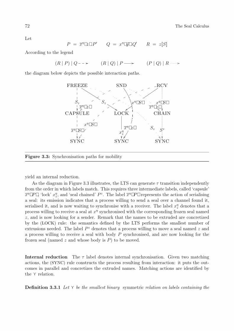
72 The Seal Calculus

LetP = xηz.P ′ Q = xη~y.Q′ R = z[S]

According to the legend

(R | P ) | Q //___ (R | Q) | P // (P | Q) | R //

the diagram below depicts the possible interaction paths.

FREEZE

Sz

���

����

Sz

��

Sz

KKKKKKKKKKKK

%%KKKKKK

SND

xηz

oq

su

}}|

xηz

xηz

��

RCV

xηS

fhik

mo

rt

wy

|�

��

�

�

xηS��

xηSuuuuuuuuuu

zzuuuuu

CAPSULE

xηS���

����

LOCK

xηz��

CHAIN

Sz

��SYNC SYNC SYNC

Figure 3.3: Synchronisation paths for mobility

yield an internal reduction.

As the diagram in Figure 3.3 illustrates, the LTS can generate τ transition independentlyfrom the order in which labels match. This requires three intermediate labels, called ‘capsule’xηP, ‘lock’ xη

z , and ‘seal chained’ P z. The label xηP represents the action of serialisinga seal: its emission indicates that a process willing to send a seal over a channel found it,serialised it, and is now waiting to synchronise with a receiver. The label xη

z denotes that aprocess willing to receive a seal at xη synchronised with the corresponding frozen seal namedz, and is now looking for a sender. Remark that the names to be extruded are concretizedby the (LOCK) rule: the semantics defined by the LTS performs the smallest number ofextrusions needed. The label P z denotes that a process willing to move a seal named z anda process willing to receive a seal with body P synchronised, and are now looking for thefrozen seal (named z and whose body is P ) to be moved.

Internal reduction The τ label denotes internal synchronisation. Given two matchingactions, the (SYNC) rule constructs the process resulting from interaction: it puts the out-comes in parallel and concretizes the extruded names. Matching actions are identified bythe g relation.

Definition 3.3.1 Let g be the smallest binary symmetric relation on labels containing the

3.3. A labelled transition semantics 73

following relation:

{ (γ1[xη1(~y)] , γ2[x

η2(~y)]) | M } ∪ { (γ1[xη1S] , γ2[x

η2S]) | M }∪ { (γ1[x

η1z ] , γ2[x

η2z]) | M } ∪ { (Sz , Sz) }

whereM def= (γ1 = η1 = γ2 = η2 = ∗)∨(γ1 = ∗ ∧ synchγ2

(η1, η2))∨(γ2 = ∗ ∧ synchγ1(η2, η1)).

Congruence rules An action observable at top-level can take place either at top-level, orinside a top-level seal. The labels keep track of where an action a takes place by tagging itwith ∗[a] if the action is a top level action, and with x[a] if the action is unleashed inside aseal x. The (SEAL LABEL) rule transforms a ∗[a] label into a x[a] label provided that theaction a can be observed from the outside of the seal x. For instance, in the process x[z[P ]]the seal z[P ] cannot be observed and this is reflected in LTS by the absence of a transition

x[z[P ]]x[Pz ]−−−−→. The rules (OPEN FREEZE) and (OPEN CAPSULE) are responsible for the

extrusion of names as a consequence of mobility actions.The remaining congruence rules are fairly standard.

3.3.1 Basic properties of the LTS

We prove some properties of the labelled transition semantics. In particular, we investi-gate how transitions are preserved and reflected by injective renaming, and we prove thecorrespondence between the LTS and the semantics in chemical style.

First of all, we remark that for a given transition A ` P`−−→ O the structure of the

process P and of the outcome O can be characterised up to structural congruence.

Lemma 3.3.2 (Transition analysis) For fn(P ) ⊆ A, consider the derivation A ` P`−−→

O.

` = ∗[xη(~z)] implies

P ≡ (ν~u)(xη(~z).R1 | R2), with x, η 6∈ ~u;

O ≡ (ν~u \ ~z)(R1 | R2);

` = a[x↑(~z)] implies

P ≡ (ν~u)(a[(ν~v)(x↑(~z).R1 | R2)] | R3), with x 6∈ (~u ∪ ~v) and a 6∈ ~u;

O ≡ (ν~u \ ~z)(a[(ν~v \ ~z)(R1 | R2)] | R3);

` = ∗[xη(~z)] implies

P ≡ (ν~u)(xη(~y).R1 | R2), with x, η, ~y, ~z 6∈ ~u;

O ≡ (ν~u)(R1[~z/~y] | R2);

` = a[x↑(~z)] implies

74 The Seal Calculus

Congruence

(PAR)

A ` P`−−→ P ′

A ` P | Q`−−→ P ′ | Q

(RES) u 6∈ fn(`)

A, u ` P`−−→ P ′

A ` (νu)P`−−→ (νu)P ′

(BANG)

A ` α.P`−−→ P ′

A ` !α.P`−−→ P | !α.P

(OPEN COM) y, η, γ 6= u;u ∈ ~x

A, u ` Pγ[yη(~x)]−−−−−−−→ P ′

A ` (νu)Pγ[yη(~x)]−−−−−−−→ P ′

(OPEN FREEZE) z 6∈ u;u ∈ fn(S)

A, u ` PSz−−−→ P ′

A ` (νu)PSz−−−→ P ′

(SEAL TAU)A ` P

τ−−→ P ′

A ` x[P ]τ−−→ x[P ′]

(OPEN CAPSULE) y, η, γ 6∈ ~u;u ∈ fn(S)

A, u ` Pγ[yηS]−−−−−−−→ P ′

A ` (νu)Pγ[yηS]−−−−−−−→ P ′

(SEAL LABEL)

A ` P∗[a]−−−−→ P ′ a ∈ {y↑(~z), y↑(~z), y↑Q, y↑Q}

A ` x[P ]x[a]−−−−→ x[P ′]

Communication(OUT)

A ` xη(~y).P∗[xη(~y)]−−−−−−→ P

(IN)

A ` xη(~y).P∗[xη(~v)]−−−−−−→ P [~v/~y]

Mobility

(SND)

A ` xηy.P∗[xηy]−−−−−−−→ P

(RCV)

A ` xη~y.P∗[xηQ]−−−−−−−→ P | y1[Q] | · · · | yn[Q]

(CAPSULE)

A ` PSz−−−→ P ′ A ` Q

∗[xηz]−−−−−−−→ Q′

A ` P | Q∗[xηS]−−−−−−−→ P ′ | Q′

(LOCK) γ = η = ∗ or (γ 6= ∗ ∧ η =↑)

A ` PSz−−−→ P ′ A ` Q

γ[xηS]−−−−−−−→ Q′

A ` P | Qγ[xη

z ]−−−−−→ (ν fn(S) \A)(P ′ | Q′)

(FREEZE)

A ` x[P ]Px−−−→ 0

(CHAIN) γ = η1 = η2 = ∗ or (η1 = γ ∧ η2 =↑)

A ` P∗[xη1y]−−−−−−−→ P ′ A ` Q

γ[xη2S]−−−−−−−−→ Q′

A ` P | QSy

−−−→ P ′ | Q′

Synchronisation

(SYNC) `1 g `2

A ` P`1−−→ P ′ A ` Q

`2−−→ Q′

A ` P | Qτ−−→ (ν(fn(`1) ∪ fn(`2)) \A)(P ′ | Q′)

The symmetric rules for (PAR), (CAPSULE), (LOCK), and (CHAIN) are omitted.

Table 3.4: A labelled transition system for the Seal Calculus

3.3. A labelled transition semantics 75

P ≡ (ν~u)(a[(ν~v)(x↑(~y).R1 | R2)] | R3), with x, ~y, ~z 6∈ (~u ∪ ~v), and a 6∈ ~u;

O ≡ (ν~u \ {a})(a[(ν~v)(R1[~z/~y] | R2)] | R3);

` = Sz implies

P ≡ (ν~u)(z[S] | R1), with z 6∈ ~u;

O ≡ (ν~u \ fn(S))R1;

` = Sz implies either

P ≡ (ν~u)(x∗z.R1 | x∗~y.R2 | R3) with z, fn(S) 6∈ ~u;

O ≡ (ν~u)(R1 | R2 | y1[S] | · · · | yn[S] | R3);

or

P ≡ (ν~u)(xaz.R1 | R2 | a[x↑~y.R3 | R4]) with z 6∈ ~u, fn(S) 6∈ ~u;

O ≡ (ν~u)(R1 | R2 | a[y1[S] | · · · | yn[S] | R3 | R4]);

` = ∗[xηy] implies

P ≡ (ν~u)(xηy.R1 | R2), with x, η, y 6∈ ~u;

O ≡ (ν~u)(R1 | R2);

` = ∗[xηS] implies

P ≡ (ν~u)(xηy.R1 | y[S] | R2), with x, η 6∈ ~u;

O ≡ (ν~u \ fn(S))(R1 | R2);

` = a[x↑S] implies

P ≡ (ν~u)(a[(ν~v)(x↑y.R1 | y[S] | R2)] | R3), with x 6∈ (~u ∪ ~v), and a 6∈ ~u;

O ≡ (ν~u \ fn(S))(a[(ν~v \ fn(S))(R1 | R2)] | R3);

` = ∗[xηS] implies

P ≡ (ν~u)(xη~y.R1 | R2), with x, η, fn(S) 6∈ ~u;

O ≡ (ν~u)(R1 | y1[S] | · · · | yn[S] | R2);

` = a[x↑S] implies

P ≡ (ν~u)(a[(ν~v)(x↑~y.R1 | R2)] | R3), with x, y, fn(S) 6∈ ~u ∪ ~v, and a 6∈ ~u;

O ≡ (ν~u \ {a})(a[(ν~v)(R1 | y1[S] | · · · | yn[S] | R2)] | R3);

` = ∗[x∗z] implies

P ≡ (ν~u)(z[S] | x∗~y.R1 | R2), with x, z 6∈ ~u;

O ≡ (ν~u)(R1 | y1[S] | · · · | yn[S] | R2);

` = a[x↑z] implies

76 The Seal Calculus

P ≡ (ν~u)(z[S] | R1 | a[(ν~v)(x↑~y.R2 | R3)]), with z 6∈ ~u, x 6∈ ~u ∪ ~v, and a 6∈ ~u;

O ≡ (ν~u)(R1 | a[(ν~v)(R2 | y1[S] | · · · | yn[S] | R3)]);

where ~u and ~v are disjoint.

Proof Induction on derivations of transitions.3 �

We now show how injective renaming preserves and reflects transitions. This theoremsare fundamental to prove that the bisimulation based equivalence that we will build on topof the LTS is preserved by injective substitutions. It is convenient to introduce some specialnotations for injective substitutions. Given an injective function f : A → B between twofinite sets of names A = {a1, . . . , an} and B, and a process P such that fn(P ) ⊆ A, wewrite fP for P [f(a1), . . . , f(an)/a1, . . . , an]. We denote dom(f) and ran(f) respectively thedomain and the range of f . Given f : A→ B and A′ ⊆ A, we write f(νA′) for f restricted toA′. Given f : A1 → B1 and g : A2 → B2 with A1∩A2 = ∅, we write f+g : A1

.∪ A2 → B1∪B2

for their set theoretic union.

Lemma 3.3.3 (Injective substitution) If A ` P`−−→ P ′, and f : A→ B and g : (fn(`) \

A)→ (N \B) are injective, then B ` fP(f+g)`−−−−−→ (f + g)P ′.

Proof Induction on derivations of transitions.

(IN) Consider A ` xη(~y).P∗[xη(~v)]−−−−−−→ P [~v/~y]. By alpha conversion, we suppose ~y 6∈ (A ∪

B ∪ (fn(`) \A)∪ ran(g)). Then f(xη(~y).P ) = fxfη(~y).fP and fn(fxfη(~y).fP ) ⊆ B. By (IN)

B ` fxfη(~y).fP∗[fxfη((f+g)~v)]−−−−−−−−−−−→ fP [(f + g)~v/~y]. Now fn(P ) ⊆ A, ~y so fn(P ) ∩ dom(g) = ∅,

so fP = (f + g)P . Hence fP [(f + g)~v/~y] = (f + g)P [(f + g)~v/~y] = (f + g)(P [~v/~y]), so we

have the transition B ` fxfη(~y).fP(f+g)∗[xη(~v)]−−−−−−−−−−→ (f + g)P [~v/~y].

(RCV) Consider A ` xη~y.P∗[xηQ]−−−−−−−→ P | y1[Q] | · · · | yn[Q]. By (RCV) B `

fxfηf~y.fP∗[fxfηQ′]−−−−−−−−−→ fP | fy1[Q

′] | · · · | fyn[Q′] for all processes Q′. In particular,

taking Q′ = (f + g)Q, B ` fxfηf~y.fP∗[fxfη(f+g)Q]−−−−−−−−−−−−→ fP | fy1[(f + g)Q] | · · · | fyn[(f +

g)Q]. As fn(P ) ⊆ A and ~y ⊆ A, we have the transition B ` f(xη~y.P )(f+g)(∗[xηQ])−−−−−−−−−−−−→

(f + g)(P | y1[Q] | · · · | yn[Q]).

(OPEN COM) Define f ′ : (A, u) → (B, g(u)) as f + (u 7→ g(u)), and g′ = g �

(fn(γ[yη(~x)]) \ {u}). By the induction hypothesis B, g(u) ` f ′P(f ′+g′)γ[yη(~x)]−−−−−−−−−−−→ (f ′ + g′)P ′,

so by (OPEN COM) B ` (νgu)f ′P(f ′+g′)γ[yη(~x)]−−−−−−−−−−−→ (f ′ + g′)P ′. So, as f ′ + g′ = f + g we have

B ` f(νu)P(f+g)γ[yη(~x)]−−−−−−−−−−→ (f + g)P ′.

(OPEN FREEZE),(OPEN CAPSULE) Similar to (OPEN COM).

(SYNC) The argument depends on the shape of the matching labels; we detail thecase when synchronisation is communication. Other cases are similar. We also suppose`2 = γ[xη2(~y)]. fn(τ) = ∅, so we have f : A → B and g : ∅ → (N \ B). Take some

3To avoid unnecessary complications in the grammar of the labels, we included the label [xηy] even ifno process can emit it.

3.3. A labelled transition semantics 77

g′ : (fn(γ2[xη2(~y)]) \ A) → (N \ B) injective. By the induction hypothesis and (COM) we

have

B ` fP(f+g′)γ1[xη1 (~y)]−−−−−−−−−−−−→ (f + g′)P ′ B ` fQ

(f+g′)γ2[xη2 (~y)]−−−−−−−−−−−−→ (f + g′)Q′

B ` f(P | Q)τ−−→ (ν((f + g′)~y) \B)(f + g′)(P ′ | Q′)

Now (f + g′)~y \ B = ran(g′), so B ` f(P | Q)τ−−→ (ν ran(g′))(f + g′)(P ′ | Q′). We have

f((ν dom(g′))(P ′ | Q′)) = (ν ran(g′))(f +g′)(P ′ | Q′), so B ` f(P | Q)τ−−→ f((ν(~y \B))(P ′ |

Q′)).

(LOCK) Similar to (SYNC).

(OUT),(SND),(FREEZE) Immediate.

(CAPSULE), (CHAIN), (PAR), (BANG), (SEAL TAU), (SEAL LABEL) Straight-forward use of the induction hypothesis. �

Lemma 3.3.4 (Shifting)

1. (A ` Pγ[xη(~u)]−−−−−−→ P ′∧v ∈ (~u\A)) if and only if (A, v ` P

γ[xη(~u)]−−−−−−→ P ′∧v ∈ ~u\ fn(P ));

2. (A ` Pγ[xηQ]−−−−−−−→ P ′ ∧ v ∈ (fn(Q) \ A)) if and only if (A, v ` P

γ[xηQ]−−−−−−−→ P ′ ∧ v ∈

fn(Q) \ fn(P ));

3. (A ` PQy

−−−→ P ′∧v ∈ (fn(Q)\A)) if and only if (A, v ` PQy

−−−→ P ′∧v ∈ fn(Q)\fn(P )).

Proof We detail the second part, others are similar (Part 3. depends on Part 2.).

We want to show that A ` Pγ[xηQ]−−−−−−−→ P ′ if and only if A, v ` P

γ[xηQ]−−−−−−−→ P ′, where

v ∈ fn(Q) \ A. We perform two inductions on derivations of transitions.

(RCV) Straightforward.

(PAR),(BANG) Straightforward use of the induction hypothesis.

(RES) Consider

A, y ` Pγ[xηQ]−−−−−−−→ P ′

A ` (νy)Pγ[xηQ]−−−−−−−→ (νy)P ′

v ∈ (fn(Q) \ A)y 6∈ γ, x, η

A, v, y ` Pγ[xηQ]−−−−−−−→ P ′

A, v ` (νy)Pγ[xηQ]−−−−−−−→ (νy)P ′

v ∈ (fn(Q) \ fn((νy)P ))y 6∈ γ, x, η

For the left-to-right implication, note that v ∈ fn(Q) \ (A, y), so by the induction hypothesis

A, v, y ` Pγ[xηQ]−−−−−−−→ P ′ and v ∈ (fn(Q) \ fn((νy)P )). For the right-to-left implication,

note that as A, v, y is well-formed we have x ∈ fn(Q) \ fn(P ), so by induction hypothesis

A, y ` Pγ[xηQ]−−−−−−−→ P ′ and v ∈ fn(Q) \ (A, y).

The other cases are vacuous. �

78 The Seal Calculus

The transitions of an injectively substituted process fP are determined by the transitionsof P as follows.

Lemma 3.3.5 (Converse to injective substitution) For f : A → B injective, if B `fP

`′−−→ Q′ then

1. there exist a label ` and a process Q,2. there exist two sets of names H, I with H ∩ I = ∅, H ∪ I = fn(`) \ A,3. there exists g : I → B′ bijective with B′ ∩B = ∅,4. there exists h : H → (B \ ran(f)) injective,

such that

a. A ` P`−−→ Q, and `′ = (f + g + h)`, and Q′ = (f + g + h)Q; and

b. if `′ 6∈ {γ[xη(~y)], γ[xηR], Ry | for some γ, x, η, ~y, R} then H = ∅.Proof Induction on derivations of transitions.

(OUT) We have B ` f(xη(~y).P )f(∗[xη(~y)])−−−−−−−−→ fP . Take Q = P , ` = ∗[xη(~y)]. Also take

H = I = ∅, g : ∅ → ∅, h : ∅ → B \ ran(f). Then A ` xη(~y).P∗[xη(~y)]−−−−−−→ P .

(IN) We can suppose without loss of generality that ~y 6∈ A ∪ B. Then we have B `

f(xη(~y).P )∗[fxfη(~z)])−−−−−−−−→ (fP )[~z/~y]. We scan ~z according to the rules below, and in doing so

we construct a new set of names ~v, and H, I, B′, g, h. Start with I = H = B′ = ∅, and g, halways undefined functions. Then, for all i:

- if zi ∈ ran(f) then vi = u for u ∈ A such that f(u) = zi;- if zi ∈ B \ ran(f) and for all j < i, zj 6= zi, then take some fresh oi such that oi 6∈ A.

Add oi to H, add h : oi 7→ zi to the current graph of h, and let vi = oi; if zj = zi forsome j < i, then let vi = vj;

- if zi 6∈ B and for all j < i, zj 6= zi, then take some new oi such that oi 6∈ A. Add oi toI, add zi to B′, add g : oi 7→ zi to the current graph of g, and let vi = oi; if zj = zi forsome j < i, then let vi = vj.

Take ` = ∗[xη(~v)], Q = P [~v/~y]. Also take the H, I, g, h constructed while generating ~v. ThenH ∩ I = ∅, H ∪ I = fn(`) \ A, g : I → B′ is a bijection, h : H → (B \ ran(f)) is injective.

Moreover, `′ = (f + g + h)`, Q′ = (f + g + h)Q, and A ` xη(~y).P∗[xη(~v)]−−−−−−→ P [~v/~y].

(SND), (FREEZE) Similar to (OUT).

(RCV) We have B ` f(xη~y.P )fxfηR′−−−−−−−→ fP | fy1[R

′] | . . . | fyn[R′]. We construct

~v, H, I, B′, g, h as we have done in (INP), but where ~z is replaced by−−−→fn(R′) (the ordering is

not important). Then let R = R′[~v/−−−→fn(R′)], and take ` = ∗[xηR], and Q = P | y1[R] | . . . |

yn[R].

(LOCK) Consider an instance

B ` fPSz−−−→ P ′ B ` fQ

γ[xηS]−−−−−−→ Q′

B ` f(P | Q)γ[xη

z ]−−−−→ (ν fn(S) \B)(P ′ | Q′)

3.3. A labelled transition semantics 79

By induction hypothesis, there exist P ′0, S0, z0 and g : (fn(S0) \ A) → B′ such that A `

PS0z0−−−−→ P ′

0 and (f + g)S0 = S, f(z0) = z, (f + g)P ′0 = P ′. This also forces H to be

empty. Again, by induction hypothesis, there exist Q′1, γ1, x1, η1, S1 and g′ : (fn(S1) \ A) →

B′ such that A ` Qγ1[x1

η1S1]−−−−−−−−−→ Q′

1 and (f + g′)S1 = S, (f + g′)Q′1 = Q′, fγ1 = γ,

fη1 = η. By Lemma 3.3.3, as g and g′ are bijection, A ` Qγ1[x1

η1S0]−−−−−−−−−→ g−1(g′(Q′

1)).

By (LINK), A ` P | Qγ1[x1

η1z1

]−−−−−−→ (ν fn(S0) \ A)(P ′ | Q′). It remains only to note that

(f + g)((ν fn(S0) \ A)(P ′0 | g−1(g′(Q′

1))) = (ν fn(S) \B)(P ′ | Q′).

(CHAIN),(CAPSULE), (SYNC) These cases are similar to (LOCK).

(PAR), (BANG), (SEAL TAU), (SEAL LABEL) By the induction hypothesis.

(RES) Consider an instance

A, u′ ` P ′ `′−−→ Q′

A ` (νu′)P ′ `′−−→ (νu′)Q′u′ 6∈ fn(`)

where fP = (νu′)P ′. There exists u 6∈ A such that P = (νu)P0 and P ′ = (f + [u′/u])P0.By the induction hypothesis there exist `, Q0, H, I and g′ : I → B′, h : H → (B \ ran(f),

where H ∪ I = fn(`) \ (A∪ {u}), such that A, u ` P0`−−→ Q0, and `′ = (f + [u′/u] + g′ + h)`,

and Q′ = (f + [u′/u] + g′ + h)Q0. Since u′ 6∈ fn(`′), it follows that u 6 fn(`). By (RES),

A ` P`−−→ (νu)Q0. The case follows taking g = g′ + [u′/u] and Q = (νu)Q0.

(OPEN COM) Consider an instance

B, u′ ` P ′ γ[yη(~x′)]−−−−−−−→ Q′

B ` (νu′)P ′ γ[yη(~x′)]−−−−−−−→ Q′

y, η, γ 6= u′; u′ ∈ ~x′

where fP = (νu′)P ′. There exist u 6∈ A and P0 such that P = (νu)P0 and P ′ = (f +[u′/u])P0. By induction hypothesis, there exist `, Q, g′ : fn(` \ (A, u))→ B′ such that A, u `P0

`−−→ Q, where ` = γ0[y0η0(~x0)], and fγ0 = γ, fy0 = y, fη0 = η and (f +g′+[u′/u])~x0 = ~x.

By (OPEN COM) A ` Pγ0[y0

η0 (~x0)]−−−−−−−−−→ Q, and the case follows taking g = g′ + [u′/u].

(OPEN FREEZE), (OPEN CAPSULE) Similar to (OPEN COM). �

Corollary 3.3.6 Let f : A → B injective, and fn(P ) ⊆ A. A ` Pτ−−→ P ′ if and only if

B ` fPτ−−→ fP ′.

To conclude this section, we state and prove the equivalence between the LTS and thesemantics in chemical style.

Lemma 3.3.7 If A ` P`−−→ Q and P ′ ≡ P then A ` P ′ `−−→ Q′ for some Q′ ≡ Q.

Proof Induction on the size of the derivation of P ′ ≡ P . �

80 The Seal Calculus

Theorem 3.3.8 Let P be a process:

1. if fn(P ) ⊆ A and A ` Pτ−−→ Q, then P _ Q;

2. if P _ Q then there exists A ⊇ fn(P ) such that A ` Pτ−−→ Q′, where Q′ ≡ Q.

Proof Both parts are proved by transition induction.

Part 1. If there is a derivation of A ` Pτ−−→ Q, then one of the following applies:

1. the last rule applied to derive A ` Pτ−−→ Q is (SYNC);

2. there are processes P ′, Q′ and a context C[−] such that P = C[P ′], Q = C[Q′], and

A ` P ′ τ−−→ Q′.

We proceed by induction on the structure of the context C[−].

Base Case There are two processes P1 and P2 such that P = P1 | P2, A ` P1`1−−→ P ′

1,

A ` P2`2−−→ P ′

2, and `1 g `2. Lemma 3.3.2 describes the structure of a process P and theoutcome O for each label ` after each transition. It remains to verify that the LTS and theg relation characterise matching processes in the reduction relation. This requires checkingall the possible matching labels in the g relation. We detail the case for `1 = ∗[xaS],`2 = a[x↑S]. Other cases are similar.

The derivation P1

∗[xaS]−−−−−−→ P ′

1 implies that P1 ≡ (ν~z)(xay.R1 | y[S] | R2) and P ′1 ≡

(ν~z \ fn(S))(R1 | R2), with x, a 6∈ ~z.

The derivation P2

a[x↑S]−−−−−−→ P ′

2 implies that P2 ≡ (ν~u)(a[(ν~v)(x↑~y.R1 | R2)] | R3) andP ′

2 ≡ (ν~u)(a[(ν~v)(R1 | y1[S] | · · · | yn[S] | R2)] | R3), with x, y, fn(S) 6∈ (~u ∪ ~v) and a 6∈ ~u.Observe that fn(S) \ A = fn(S) ∩ ~z. It holds

P1 | P2 ≡ (ν~z)(xay.R1 | y[S] | R2) | (ν~u)(a[(ν~v)(x↑~y.R1 | R2)] | R3)

_ (ν(fn(S) ∪ {a}) \ A)((ν~z \ fn(S))(R1 | R2)

| (ν~u)(a[(ν~v)(R1 | y1[S] | · · · | yn[S] | R2)] | R3))

≡ P ′1 | P ′

2 .

Inductive step Follows easily from the congruence laws of reduction.

Part 2. We detail one of the base cases, the others are similar. Rule (move out) says:

xa~u.P | a[(ν~z)(x↑v.Q1 | v[R] | Q2)]

_ (ν fn(R) ∩ ~z)(P | u1[R] | · · · | un[R] | a[(ν~z \ fn(R))(Q1 | Q2)])

where x 6∈ ~z. Let A = fn(P ). From the LTS, we can derive:

1. A ` xa~u.P∗[xaR]−−−−−−−→ P | u1[R] | · · · | un[R]

3.4. A proof method 81

2. As x 6∈ ~z the following is a valid derivation:

A ` x↑v.Q1

∗[x↑v]−−−−−−→ Q1 A ` v[R]

Rv−−−→ 0

A ` x↑v.Q1 | v[R]∗[x↑R]−−−−−−→ Q1 | 0

A ` x↑v.Q1 | v[R] | Q2

∗[x↑R]−−−−−−→ Q1 | 0 | Q2

A ` (ν~z)(x↑v.Q1 | v[R] | Q2)∗[x↑R]−−−−−−→ (ν~z \ fn(R))(Q1 | 0 | Q2)

A ` a[(ν~z \ fn(R))(x↑v.Q1 | v[R] | Q2)]a[x↑R]−−−−−−−→ a[(ν~z \ fn(R))(Q1 | 0 | Q2)]

As ∗[xaR]g a[x↑R], we can apply the rule (SYNC) to derive

A ` xa~u.P | a[(ν~z)(x↑v.Q1 | v[R] | Q2)]τ−−→ (ν fn(R) ∩ ~z)(P | u1[R] | · · · | un[R] | a[(ν~z \ fn(R))(Q1 | 0 | Q2)])

as desired.To complete the inductive step, observe that the congruence cases follow because the

label τ can cross every context (rules (PAR), (RES), (SEAL TAU)), and the insensitivity tostructural congruence follows from Lemma 3.3.7. �

3.4 A proof method

In this section we use the LTS defined in the previous section to define a bisimulation basedrelation contained in reduction barbed congruence. This will be an useful proof method toensure equivalence between terms, and will be subsequently used to explore the behaviouraltheory of S -Seal. At the same time, its development will point out some peculiarities of Sealsemantics.

3.4.1 LTS and observable actions

We first reexamine the definition of reduction barbed congruence, and we show that it isvery robust under changes to the precise definition of barbs.

The predicate P ↓ n detects the ability of a process P to interact with the environment viathe seal n. In other process calculi, like the π-calculus, barbs are defined using visible actions.We show that reduction barbed congruence is not affected if we change our definition of barbwith barbs inherited from the visible actions of the LTS. We refer to barbs of Definition 3.2.3as natural barbs.

First, we remark that the exposure of a barb corresponds to the emission of a ‘freeze’label in the labelled transition system:

Lemma 3.4.1 P ↓ n if and only if A ` PQn−−−→ P ′ for some P ′, Q, and A, with fn(P ) ⊆ A.

Proof The ‘if’ part is a consequence of Lemma 3.3.2, while the ‘only if’ part followsstraightforwardly from Definition 3.2.5. �

82 The Seal Calculus

C∗[x∗y][−] = y[a↑()] | x∗i.ai().o[ ] | − C∗[x∗z ][−] = x∗z.o[ ] | −C∗[x↑y][−] = y[a↑()] | xui.ai().o[ ] | u[− ] Ck[x↑z ][−] = xkz.o[ ] | −

C∗[x∗S][−] = a[S] | x∗a.o[ ] | − C∗[x∗?][−] = x∗a.o[ ] | −C∗[x↑S][−] = a[S] | xua.o[ ] | u[− ] C∗[x↑?][−] = xua.o[ ] | u[− ]

Ck[x↑S][−] = a[S] | xka.o[ ] | − Ck[x↑?][−] = xka.o[ ] | −

where a, i, o, u are fresh names.

Table 3.5: Contexts that transform a λ-barb into a natural barb

We now prove that for all classes of visible actions of our LTS the resulting definitionsof barbed congruence collapse and coincide with ∼=. For that we classify the actions of theLTS according to the axiom or rule responsible for generating them (that is, according totheir ‘shape’):

Definition 3.4.2 (λ-barbs) We define the following sets of actions

L∗SND∗ = { ∗[x∗y] | for all x, y } L∗LOCK∗ = { ∗[x∗z] | for all x, z }L∗SND↑ = { ∗[x↑y] | for all x, y } L∗LOCK↑ = { ∗[x↑z] | for all x, z }

L∗RCV∗ = { ∗[x∗S] | for all x, S } W∗CAPS∗ = { ∗[x∗S] | for all x, S }L∗RCV↑ = { ∗[x↑S] | for all x, S } W∗CAPS↑ = { ∗[x↑S] | for all x, S }LkRCV↑ = { k[x↑S] | for all x, S } WkCAPS↑ = { k[x↑S] | for all x, S }

ans we refer to each of them as a class of actions.

Let L =⋃

λ Lλ. For ω ∈ L, we write P ↓ ω if Pω−−→, and P ⇓ ω if P ⇒ ω−−→.

LetW =⋃

λWλ. We write P ↓ γ[xη?] if there exists a process S such that Pγ[xηS]−−−−−−−→.

We write P ⇓ γ[xη?] if there exists a process S such that P ⇒γ[xηS]−−−−−−−→.

Let A = L∪W, and let λ range over the classes of actions. We call λ-barbs all the barbsthat belong to the class λ.

Definition 3.4.3 For each class of actions λ, let ∼=λ be the largest congruence over processesthat is reduction closed and preserves λ-barbs.

For example, if P ∼=∗SND∗ Q and P ↓ ∗[a∗z] (that is, P∗[a∗z]−−−−−−→), then Q ⇓ ∗[a∗z] (that

is, Q⇒∗[a∗z]−−−−−−→). And if P ∼=∗CAPS∗ Q and P ↓ ∗[a∗?] (that is, P

∗[a∗R]−−−−−−→ for some R),

then Q ⇓ ∗[a∗?] (that is, Q⇒∗[a∗S]−−−−−−→ for some S).

3.4. A proof method 83

D∗[x∗y]n [−] = − | a∗n | a∗n.x∗y D∗[x∗z ]

n [−] = − | a∗n | a∗n.(x∗z | z[0])

D∗[x↑y]n [−] = − | a∗n | a∗n.x↑y Dk[x↑z ]

n [−] = − | a∗n | a∗n.(k[x∗z] | z[0])

D∗[x∗S]n [−] = − | a∗n | a∗n.x∗ D∗[x∗?]

n [−] = − | a∗n | a∗n.x∗0

D∗[x↑S]n [−] = − | a∗n | a∗n.x↑ D∗[x↑?]

n [−] = − | a∗n | a∗n.x↑0

Dk[x↑S]n [−] = − | a∗n | a∗n.k[x↑] Dk[x↑?]

n [−] = − | a∗n | a∗n.k[x↑0]

where a is a fresh name.

Table 3.6: Contexts that transform a natural barb into a λ-barb

Lemma 3.4.4 Consider the contexts defined in Table 3.5. Then Cω[P ] ⇓ o if and only ifP ⇓ ω.

Proof The if direction is a direct consequence of Lemma 3.3.2.For the only if direction, the proof depends on the action ω. The main argument is that

the process Cω[P ] can unleash the seal named o only if P performs the action ω.The most interesting case is when ω = ∗[x∗y]. The term

C∗[x∗y][P ] = y[a↑()] | x∗i.ai().o[ ] | P

must consume the two actions x∗i and ai() to activate the seal named o. The first onesynchronises either with x∗y (as we desire) or x∗S. In this last case the moved seal isprovided by P and it cannot perform an interaction over the channel a, that has been chosenfresh for P . In turn, the second action can be consumed only if the seal y provided by thecontext is moved and renamed into i. This guarantees that P ⇓ x∗y.

The other cases are simpler. �

Lemma 3.4.5 Consider the contexts defined in Table 3.6. Then Dωn [P ] ⇓ ω if and only if

P ⇓ n.

Proof Each context can be rewritten as − | a∗n | a∗n.X where X is depends on theparticular context. As the name a is fresh, the prefix a∗n is consumed only if the processthat fills the hole offers a seal named n at top-level, that is, it emits ↓ n. The continuationX is then responsible for generating the appropriate λ-barb. �

Theorem 3.4.6 Let P and Q be two processes, and let λ be a class of actions. Then P ∼= Qif and only if P ∼=λ Q.

Proof Since ∼= and ∼=λ differ only in the barb which is used, it suffices to show ↓ n and↓ λ imply each other.

First we prove that P ∼=λ Q implies P ∼= Q. Let P ∼= Q and P ↓ ω for ω ∈ λ. We want toconclude that Q ⇓ ω. As ∼= is contextual, it holds Cω[P ] ∼= Cω[Q]. Lemma 3.4.4 guarantees

84 The Seal Calculus

that Cω[P ] ⇓ o. As ∼= preserves natural barbs, it must hold Cω[Q] ⇓ o. Lemma 3.4.4 allowsus to conclude Q ⇓ ω.

For the other implication, suppose P ∼=λ Q and P ↓ n. We want to conclude that Q ⇓ n().Let ω be a label in λ. As ∼=λ is contextual, it holds Dω

n [P ] ∼= Cωn [Q]. Lemma 3.4.5 guarantees

that Cωn [P ] ⇓ ω. As ∼= preserves λ-barbs, it must hold Cω

n [Q] ⇓ ω. Lemma 3.4.5 allows us toconclude Q ⇓ n. �

To shorten the presentation, in the Definition of λ-barbs we did not include actionsrelated to communication. Unsurprisingly, the Theorem above can easily be expanded totake into account also barbs exposing communication actions.

Theorem 3.4.6 brings out two peculiarities of the LTS proposed. First, the class of actiongenerated by the (Chain) rule do not appear among the classes for which reduction λ-barbedcongruence coincides with reduction barbed congruence. As we will discuss in Section 3.4.3,these actions cannot be observed by a context. Second, analogously to what happens withnatural barbs, the classes of action γCAPSη do not report the body of the moved seal intheir prototypical action. This is typical of our treatment of some of the higher order actions,where weak matching requirements on the transmitted processes are imposed.

3.4.2 Higher-order actions and bisimulation

Lemma 3.4.1 shows that the observation used in the contextual equivalence is insensitiveto the particular process Q occurring in the label of the corresponding ‘freeze’ transition.Thus we expect a LTS based characterisation of this equivalence not to be strict in matchinghigher-order labels.

To avoid the difficulties we pointed out in the introduction we resort to the intuitionunderlying the definition of Sangiorgi’s context bisimulation for HO-π [San92, San96a], andrequire that the outcomes of two bisimilar processes emitting higher order transitions mustbe equivalent with respect to every possible interaction with a context.

Processes appear in four kinds of higher-order labels: γ[xηS], Sz, Rz, and γ[xηR].We focus on the contexts with which a process emitting a higher-order label can interact,with the aim of finding out how to apply context bisimulation to our framework.

Receiving a seal body Suppose that A ` Pγ[xηS]−−−−−−→ P ′, and let Q be a process supposed

equivalent to P . The process P ′ is the outcome of the interaction between P and a contextC[−] sending a seal body S over the channel xη. In the bisimulation game, the processQ must be able to receive an arbitrary seal body over the channel xη, otherwise a contextcan easily separate P from Q. At the same time, it should be stressed that the process Sappearing in the label is offered by the context, and as such the processes P and Q mustboth be ready to receive it. Therefore when comparing processes that receive a seal body, itis not restrictive to require syntactically identical processes in higher-order labels.

The case for Sz is analogous to the previous one, as the process S is offered by theenvironment.

3.4. A proof method 85

Emitting a seal body Suppose that A ` PRz−−−→ P ′. This can be seen as the offer

of an interaction with a context that can move and/or duplicate the seal z. We must at

least require that there exists a process Q′ such that A ` QSz−−−→ Q′ for some seal body

S, otherwise a context can easily separate P from Q. At the same time, imposing S to besyntactically the same as R is overly restrictive. This is a consequence of the fact that thecontext can not directly investigate the seal body S, but it must move and/or duplicate itbefore being able to interact with it. Thus, we do not impose directly any condition on S.Rather, we ask that the outcomes obtained after interacting with an arbitrary context thatreceives (that is, moves and/or copies) the seal are equivalent.

The case for xηR is similar: the only advantage is that it is known where the interactingcontext is going to reactivate the copies of the seal.

To state the equivalence of processes emitting a seal body, we must characterise all thepossible outcomes obtained after an interaction between a mobility offer and a context willingto receive the seal body being sent. This role is played by the receiving contexts.

Receiving contexts represent all the processes that may result from the migration of aseal. An example is probably helpful here. Let A be a set of names. In this ‘universe’,consider a process P that emits the label z[x↑R] and becomes P ′:

A ` Pz[x↑R]−−−−−−→ P ′ .

A context that synchronises with P over this label must have the shape C ′[−] ≡ C[ − |xz~y.V ], for some C[−] and V . The resulting reduction is

C ′[P ] ≡ C[ P | xz~y.V ] _ C[ (ν fn(R) \ A)(P ′ | y1[R] | · · · | yn[R] | V ) ] .

The process V cannot know any name in fn(R) \ A, so we rewrite the above reduction as

C[ P | xz~y.V ] _ C[ (ν fn(R) \ A)(P ′ | y1[R] | · · · | yn[R]) | V ] . (3.3)

Our aim is to define a bisimulation based equivalence, ≈, such that contexts like C ′[−] cannotdistinguish equivalent processes. In the example above, this means that the process C ′[Q]must reduce to a process equivalent to the outcome of (3.3). An easy way to achieve this isto require that in the bisimulation game Q emits a label that consumes the action xz~y.V ,that is

A ` Qz[x↑S]−−−−−−→ Q′ for some S, Q′,

and that the outcome of C ′[P ] is equivalent to the outcome of C ′[Q]:

C[ (ν fn(R) \A)(P ′ | y1[R] | · · · | yn[R]) | V ] ≈ C[ (ν fn(S) \A)(Q′ | y1[S] | · · · | yn[S]) | V ]

Some housekeeping now: we factor out the context common to both members of the equation,C[[−] | V ], and we check that the following equivalence holds:

(ν fn(R) \ A)(P ′ | y1[R] | · · · | yn[R]) ≈ (ν fn(S) \ A)(Q′ | y1[S] | · · · | yn[S]) .

This idea can be generalised. Consider two processes (like P and Q) that in an universeA send two (possibly different) seal bodies from a location z toward their parent ↑. We

86 The Seal Calculus

consider these two processes as equivalent only if the substitutions of the sent seal bodiesfor Y and of the outcomes for X in the following pattern

(ν fn(Y ) \ A)(X | y1[Y ] | · · · | yn[Y ])

yield equivalent processes. The pattern process above is called a receiving context, from ztoward ↑ in A, and is noted as DA

z,↑[X,Y ]. Its associated environment is the set of freevariables of the process obtained after instantiating X and Y .

Definition 3.4.7 (Receiving Context) Let A be a set of variables. Given two processesX and Y such that fn(X) ⊆ A, a receiving context DA

γ,η[X, Y ] and its associated environmentADA

γ,η [X,Y ] are respectively a process and a set of names defined as:

if γ, η = ∗, ∗, or γ, η = z, ↑, then

DAγ,η[X, Y ] = (ν fn(Y ) \ A)( X | z1[Y ] | · · · | zn[Y ] )

where the names ~z satisfy fn(DAγ,η[X, Y ]) ⊆ A ∪ ~z.

Its associated environment ADAγ,η [X,Y ] is A ∪ ~z;

if γ, η = ∗, z, then

DA∗,z[X, Y ] = (ν fn(Y ) \ A)( X | z[( z1[Y ] | · · · | zn[Y ] | U )] )

where the names ~z and the process U satisfy fn(DA∗,z[X, Y ]) ⊆ A ∪ ~z.

Its associated environment ADA∗,z [X,Y ] is A ∪ ~z;

if γ, η = ∗, ↑, thenDA∗,↑[X, Y ] = z[X | U ] | z1[Y ] | · · · | zn[Y ]

where the names z, ~z and the process U satisfy fn(DA∗,↑[X, Y ]) ⊆ A ∪ ~z ∪ {z}.

Its associated environment ADA∗,↑[X,Y ] is A ∪ ~z ∪ {z}.

We write DA[X,Y ] when we quantify over all γ, η and abbreviate ADAγ,η [X,Y ] by AD when no

ambiguity arises.

Seal bisimulation According to our analysis, we are now ready to define a bisimulationbased equivalence relation over seal processes.

Definition 3.4.8 (Bisimilarity) Let bisimilarity, denoted ≈, be the largest family of re-lations indexed by finite sets of names such that each ≈A is a symmetric relation over{P | fn(P ) ⊆ A} and for all P ≈A Q the following conditions hold:

1. if A ` Pτ−−→ P ′ then there exists a Q′ such that A ` Q⇒ Q′ and P ′ ≈A Q′;

2. if A ` P`−−→ P ′ and ` ∈ { γ[xη(~y)], γ[xη(~y)], ∗[xηy], γ[xηS], Sz, γ[xη

z ] }, then there

exists a Q′ such that A ` Q⇒ `−−→ Q′ and P ′ ≈A∪fn(`) Q′;

3.4. A proof method 87

3. if A ` PRz−−−→ P ′ then there exist Q′, S such that A ` Q⇒ Sz−−−→ Q′ and for all admissible

contexts DA[−,−] it holds DA[P ′, R] ≈AD DA[Q′, S];

4. if A ` Pγ[xηR]−−−−−−−→ P ′ then there exist Q′, S such that A ` Q⇒

γ[xηS]−−−−−−−→ Q′ and for all

admissible contexts DAγ,η[−,−] it holds DA

γ,η[P′, R] ≈AD DA

γ,η[Q′, S];

5. for all substitutions σ such that dom(σ) ⊆ A and ran(σ) ⊆ A, Pσ ≈A Qσ;

where a context DA[−,−] is admissible if both process substitutions DA[P ′, R] and DA[Q′, S]are well-formed (i.e. no name capture arises).

Intuitively, the first two cases of Definition 3.4.8 handle all first-order labels, as well aslabels originating from receive actions: these do not deserve a special treatment because ourearly semantics implicitly tests all possible interactions. The cases 3. and 4. check processesthat offer a seal body. Condition 5. ensures that ≈ is preserved by contexts where the holein under a input prefix.

Standard reasoning, albeit here for an indexed relation, guarantees that

Proposition 3.4.9 The relation ≈ exists uniquely and is an equivalence.

Bisimilarity is preserved by all the constructors of the calculus, albeit working with anindexed relation requires a little care even to state the congruence property, to keep theA-indexing straight. Following [Sew00], we resort to the notion of indexed congruence.

Definition 3.4.10 (Indexed congruence) Consider a family R of relations indexed byfinite sets of names such that each RA is a relation over {P | fn(P ) ⊆ A}. R is an indexedcongruence if each RA is an equivalence relation and the following hold:

P RA,~y Q x, fn(η) ⊆ A

xη(~y).P RA xη(~y).Q

P RA Q α 6= xη(y), fn(α) ⊆ A

α.P RA α.Q

P RA,~y Q x, fn(η) ⊆ A

!xη(~y).P RA !xη(~y).Q

P RA Q α 6= xη(y), fn(α) ⊆ A

!α.P RA !α.Q.

P RA Q x ∈ A

x[P ] RA x[Q]

P RA Q fn(R) ⊆ A

P | R RA Q | RR | P RA R | Q

P RA,x Q

(νx)P RA (νx)Q

Our aim here is to prove that bisimilarity is an indexed congruence. It is easier to proveseparately that bisimilarity is preserved by the different constructs of the language. Beforeproceeding, we introduce an elementary but useful up-to proof technique.

Lemma 3.4.11 If R is a bisimulation up to structural congruence, then R ⊆ ≈.

Proof Let SA = {(P, Q) | (P1, Q1) ∈ RA, P1 ≡ P and Q1 ≡ Q}, where A is a set of names.Clearly, for every A, it holds RA ⊆ SA, and

⋃ARA ⊆

⋃A SA. Because of Lemma 3.3.7, a

diagram chasing argument allows us to show that for every set of names A, the relation SAis closed under the conditions to be a bisimulation, as required. �

88 The Seal Calculus

Lemma 3.4.12 If P ≈A Q, then x[P ] ≈A x[Q] for all x ∈ A.

Proof Define SA = {(x[P ], x[Q]) | P ≈A Q, x ∈ A} ∪ ≈A and let S =⋃

A SA. Weshow that S is a bisimulation. Consider (R,S) ∈ S. Then there exists A such that eitherR ≈A S holds, or R = x[P ] and S = x[Q] for x ∈ A and P ≈A Q. In the former case theresult follows straightforwardly. We next consider the possible transitions in the latter case.A simple inspection of the rules of LTS shows that if x[P ] emits a label, then one of thefollowing cases holds:

• A ` x[P ]x[a]−−−→ x[P ′] for some P ′, where a ∈ {τ, y↑(~z), y↑(~z), y↑Q} and A ` P

∗[a]−−−→

P ′. We have A ` Q ⇒∗[a]−−−→ Q′ and P ′ ≈A∪fn(a) Q′ because of the definition of

bisimulation. Since x ∈ A, we have A ` x[Q] ⇒x[a]−−−→ x[Q′], and x[P ′] SA∪fn(a) x[Q′]

follows from the definition of S.

• A ` x[P ]x[y↑R]−−−−−−−→ x[P ′] for some P ′, where A ` P

∗[y↑R]−−−−−−→ P ′. The defini-

tion of bisimulation ensures that (i) A ` Q ⇒∗[y↑S]−−−−−−→ Q′ for some Q′, S; and (ii)

DA∗,↑[P

′, R] ≈AD DA∗,↑[Q

′, S] for every possible such a pair of receiving contexts. From

(i) we deduce that A ` x[Q] ⇒x[y↑S]−−−−−−→ x[Q′]. Now use (ii) and notice that every

process that is a receiving context DAx,↑[x[O],−] is also a receiving context DA

∗,↑[O,−].Therefore (ii) implies that DA

x,↑[x[P ′], R] ≈AD DAx,↑[x[Q′], S], which, by definition of

S impliesDA

x,↑[x[P ′], R] SAD DAx,↑[x[Q′], S] .

The last property we have to check for is closure under substitutions. Let σ be a substitutiondefined on A. Let (R,S) ∈ S. Then there exists A such that either R ≈A S holds, orR = x[P ] and S = x[Q] for x ∈ A and P ≈A Q. In the first case Pσ ≈Aσ Qσ holds because≈ is closed under arbitrary substitution. Then Pσ SAσ Qσ follows from the construction of S.In the latter, observe that xσ ∈ Aσ because x ∈ A, and Rσ ≈Aσ Sσ holds because ≈ is closedunder arbitrary substitution. The definition of substitution assures that xσ[Rσ] = (x[R])σand xσ[Sσ] = (x[S])σ. Then (x[R])σ SAσ (x[S])σ follows because of the construction ofS. �

Lemma 3.4.13 If P ≈A Q, then P | R ≈A Q | R and (νx)P ≈A\x (νx)Q, for all x ∈ A,and for all R such that fn(R) ⊆ A.

Proof Define SA = {( (ν~u)(P | R) , (ν~u)(Q | R) ) P ≈A,~u Q, (fn(R) \ ~u) ⊆ A},and let S =

⋃A SA. We show that S is a bisimulation up to structural congruence. Suppose

P ≈A Q. As a useful shorthand, we write P for (ν~u)(P | R), and Q for (ν~u)(Q | R).We perform a case analysis on the transitions performed by P . We detail all the most dif-

ficult and interesting situations (namely higher-order synchronisation and scope extrusion):the others follow accordingly.

• Suppose A ` Pγ[xη

z ]−−−−→ O1 because A · ~u ` P

γ[xηF ]−−−−−−−→ P ′ and A · ~u ` R

Fz−−−→ R′.

From the definition of bisimulation it follows that A · ~u ` Q⇒γ[xηF ]−−−−−−−→ Q′ and

P ′ ≈A∪~u∪fn(F ) Q′ . (3.4)

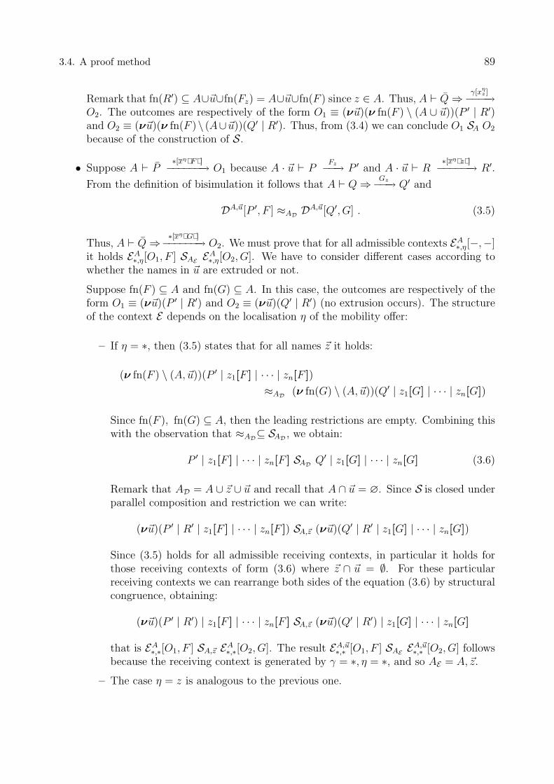
3.4. A proof method 89

Remark that fn(R′) ⊆ A∪~u∪fn(Fz) = A∪~u∪fn(F ) since z ∈ A. Thus, A ` Q⇒γ[xη

z ]−−−−→

O2. The outcomes are respectively of the form O1 ≡ (ν~u)(ν fn(F ) \ (A ∪ ~u))(P ′ | R′)and O2 ≡ (ν~u)(ν fn(F )\ (A∪~u))(Q′ | R′). Thus, from (3.4) we can conclude O1 SA O2

because of the construction of S.

• Suppose A ` P∗[xηF ]−−−−−−−→ O1 because A · ~u ` P

Fz−−−→ P ′ and A · ~u ` R∗[xηz]−−−−−−→ R′.

From the definition of bisimulation it follows that A ` Q⇒ Gz−−−→ Q′ and

DA,~u[P ′, F ] ≈AD DA,~u[Q′, G] . (3.5)

Thus, A ` Q⇒∗[xηG]−−−−−−−→ O2. We must prove that for all admissible contexts EA

∗,η[−,−]it holds EA

∗,η[O1, F ] SAE EA∗,η[O2, G]. We have to consider different cases according to

whether the names in ~u are extruded or not.

Suppose fn(F ) ⊆ A and fn(G) ⊆ A. In this case, the outcomes are respectively of theform O1 ≡ (ν~u)(P ′ | R′) and O2 ≡ (ν~u)(Q′ | R′) (no extrusion occurs). The structureof the context E depends on the localisation η of the mobility offer:

– If η = ∗, then (3.5) states that for all names ~z it holds:

(ν fn(F ) \ (A, ~u))(P ′ | z1[F ] | · · · | zn[F ])

≈AD (ν fn(G) \ (A, ~u))(Q′ | z1[G] | · · · | zn[G])

Since fn(F ), fn(G) ⊆ A, then the leading restrictions are empty. Combining thiswith the observation that ≈AD⊆ SAD , we obtain:

P ′ | z1[F ] | · · · | zn[F ] SAD Q′ | z1[G] | · · · | zn[G] (3.6)

Remark that AD = A ∪ ~z ∪ ~u and recall that A ∩ ~u = ∅. Since S is closed underparallel composition and restriction we can write:

(ν~u)(P ′ | R′ | z1[F ] | · · · | zn[F ]) SA,~z (ν~u)(Q′ | R′ | z1[G] | · · · | zn[G])

Since (3.5) holds for all admissible receiving contexts, in particular it holds forthose receiving contexts of form (3.6) where ~z ∩ ~u = ∅. For these particularreceiving contexts we can rearrange both sides of the equation (3.6) by structuralcongruence, obtaining:

(ν~u)(P ′ | R′) | z1[F ] | · · · | zn[F ] SA,~z (ν~u)(Q′ | R′) | z1[G] | · · · | zn[G]

that is EA∗,∗[O1, F ] SA,~z EA

∗,∗[O2, G]. The result EA,~u∗,∗ [O1, F ] SAE EA,~u

∗,∗ [O2, G] followsbecause the receiving context is generated by γ = ∗, η = ∗, and so AE = A, ~z.

– The case η = z is analogous to the previous one.

90 The Seal Calculus

– If η =↑ then from (3.5), case γ, η = ∗, ↑ we can deduce that for all U ′ it holds

z[P ′ | R′ | U ′] | z1[F ] | · · · | zn[F ] ≈A∪~z∪~u z[Q′ | R′ | U ′] | z1[G] | · · · | zn[G]

(it suffices to take U = U ′ | R′). The construction of S then guarantees that

(ν~u)z[P ′ | R′ | U ′] | z1[F ] | · · · | zn[F ]

≈A∪~z (ν~u)z[Q′ | R′ | U ′] | z1[G] | · · · | zn[G]

and up to structural congruence we obtain

z[(ν~u)(P ′ | R′ | U ′)] | z1[F ] | · · · | zn[F ]

≈A∪~z z[(ν~u)(Q′ | R′ | U ′)] | z1[G] | · · · | zn[G] .

This can be written using receiving contexts as EA∗,↑[O1, F ] SAE EA

∗,↑[O2, G], asrequired.

Suppose now that fn(F ) 6⊆ A and fn(G) ⊆ A. This means that in P some of thenames in ~u are extruded by the mobility offer. condition As before, we perform a caseanalysis on the localisation η. We detail only the case η = ∗: the others are similar.If η = ∗, then the outcomes are respectively of the form O1 ≡ (ν~u \ fn(F ))(P ′ | R′)and O2 ≡ (ν~u)(Q′ | R′). We spell out (3.5) for γ, η = ∗, ∗. It holds P ′ | z1[F ] | · · · |zn[F ] ≈A∪~u∪~z Q′ | z1[G] | · · · | zn[G]. This implies that for all ~z it holds

(ν~u)(P ′ | R′ | z1[F ] | · · · | zn[F ]) SA∪~z (ν~u)(Q′ | R′ | z1[G] | · · · | zn[G])

Now notice that since A ` P = (ν~u)(P | R)∗[xηF ]−−−−−−−→ then F occurs in P and therefore

fn(F ) ⊆ A∪~u. From the last formula we obtain fn(F )\A ⊆ ~u from which it is possibleto deduce that ~u = (fn(F ) \ A) ∪ (~u \ fn(F )). Therefore we have:

(ν fn(F ) \ A)(ν~u \ fn(F ))(P ′ | R′ | z1[F ] | · · · | zn[F ] )

SA∪~z (ν~u)(Q′ | R′ | z1[G] | · · · | zn[G] )

Since the equation above holds for all ~z, then in particular it holds for those ~z suchthat ~u ∩ ~z = ∅. In this case then we can extrude the zi’s from the scope of the innerrestriction in the left hand-side of the above equation above. Furthermore recall thatA ∩ ~u = ∅ and fn(G) ⊆ A, which implies fn(G) ∩ ~u = ∅. Then we can extrude theseseals in the right hand-side,too. Up to structural congruence we have:

(ν fn(F ) \ A)( ((ν~u \ fn(F ))(P ′ | R′)) | z1[F ] | · · · | zn[F ] )

SA∪~z (ν~u)(Q′ | R′) | z1[G] | · · · | zn[G]

that is EA∗,∗[O1, F ] SAE EA

∗,∗[O2, G].

Finally, the remaining two cases, that is fn(F ) ⊆ A, fn(G) 6⊆ A and fn(F ) 6⊆ A,fn(G) 6⊆ A, are similar to the previous one.

3.4. A proof method 91

• Suppose A ` Pτ−−→ O1, where A · ~u ` P

Fz−−−→ P ′ and A · ~u ` RF z

−−−→ R1.By Lemma 3.3.2 either R1 ≡ (ν ~w)(R3 | z1[F ] | · · · | zn[F ]) or R1 ≡ (ν ~w)(R3 |z[R4 | z1[F ] | · · · | zn[F ]]) hold. From the definition of bisimulation it follows that

A · ~u ` Q⇒ Gz−−−→ Q′, and for all DA,~u[−,−] admissible it holds

DA,~u[P ′, F ] ≈AD DA,~u[Q′, G]. (3.7)

The early nature of the LTS allows process R to receive G as well: A · ~u ` RGz

−−−→ R2,with R2 either in the form R2 ≡ (ν ~w)(R3 | z1[G] | · · · | zn[G]), or R2 ≡ (ν ~w)(R3 |z[R4 | z1[G] | · · · | zn[G]]). Thus, A ` Q⇒ τ−−→ O2.

Consider the first case.

Before going on, we point out that as A · ~u ` RF z

−−−→≡ (ν ~w)(R3 | z1[F ] | · · · | zn[F ]),the condition ~z ⊆ A∪~u∪ ~w must hold. Also, fn(R3) ⊆ A∪~u∪ ~w. To see why, rememberthat R3 is formed by the parallel composition of two residuals: the continuation of thereceiving action, and the continuation of the send action. The free variables of the firstprocess must be contained in A∪~u∪~z∪{x} where x is the channel on which the movetakes place; those of the second process are instead contained in A ∪ ~u ∪ {z} ∪ {x}.Thus fn(R3) ⊆ A ∪ ~u ∪ ~z ∪ {z} ∪ {x}. But {z} ∪ {x} ⊆ A ∪ ~u as they obviously occurfree in the sending process (cf. rule (SND)). So, ~z ⊆ A ∪ ~w and we conclude thatfn(R3) ⊆ A ∪ ~u ∪ ~w.

The outcomes are respectively of the form

O1 ≡ (ν~u)(ν fn(F ) \ (A ∪ ~u))(P ′ | (ν ~w)(R3 | z1[F ] | · · · | zn[F ] ))

O2 ≡ (ν~u)(ν fn(G) \ (A ∪ ~u))(Q′ | (ν ~w)(R3 | z1[G] | · · · | zn[G] )) .

Since fn(R3) ⊆ A ∪ ~u ∪ ~w we have fn(R3) ∩ (fn(F ) \ (A ∪ ~u)) = ∅, and similarlyfn(R3) ∩ (fn(G) \ (A ∪ ~u)) = ∅. We can then extrude R3 from the scope of the innerrestriction as follows:

O1 ≡ (ν~u)(ν ~w)(R3 | (ν fn(F ) \ (A ∪ ~u))(P ′ | z1[F ] | · · · | zn[F ] ))

O2 ≡ (ν~u)(ν ~w)(R3 | (ν fn(G) \ (A ∪ ~u))(Q′ | z1[G] | · · · | zn[G] )) .

The case γ, η = ∗, ∗ of (3.7) implies that

(ν fn(F ) \ (A ∪ ~u))(P ′ | z1[F ] | · · · zn[F ] )

≈A∪~z∪~u (ν fn(G) \ (A ∪ ~u))(Q′ | z1[G] | · · · zn[G] ) (3.8)

The construction of S allows us to derive O1 S(A∪~u∪~z)\(~u∪~w) O2 from 3.8. As ~z ⊆A ∪ ~u ∪ ~w, (A ∪ ~u ∪ ~z) \ (~u ∪ ~w) = A, and we conclude O1 SA O2, as required.

The latter case follows accordingly. �

Theorem 3.4.14 Bisimilarity is an indexed congruence.

Proof It is straightforward to prove that ≈ is preserved by prefix and replication. Theother cases are covered by Lemma 3.4.12 and Lemma 3.4.13.4 �

4The proof of the symmetric case of congruence with respect to parallel composition is analogous to theproof of Lemma 3.4.13.

92 The Seal Calculus

Lemma 3.4.15 (Injective substitution — bisimulation) If P ≈A Q and f : A→ B isinjective then fP ≈B fQ.

Proof We check

RB = { (fP, fQ) | f : A→inj B and P ≈A Q }

is a bisimulation.

Suppose B ` fP`′−−→ P ′

1. We perform a case analysis on the label `′.

Case ` = τ . By Corollary 3.3.6, there exists P ′ such that A ` Pτ−−→ P ′ and P ′

1 = fP ′.By bisimulation, there exists Q′ such that A ` Q ⇒ Q′ and P ′ ≈A Q′. By Corollary 3.3.6,B ` fQ⇒ fQ′. Finally fP ′RBfQ′.

Case ` ∈ { γ[xη(~y)], γ[xη(~y)], ∗[xηy], γ[xηS], Sz, γ[xηz ] }. By Lemma 3.3.5, there exist

`, P ′, H, I, g : I →bij B′, h : H →inj (B \ ran(f)) : such that B′ ∩ B = ∅, H ∪ I = fn(`) \ A,H ∩ I = ∅, and

A ` P`−−→ P ′ P ′

1 = (f + g + h)P ′ `′ = (f + g + h)` .

By bisimulation, there exists Q′ such that A ` Q⇒ l−→ Q′ and P ′ ≈A∪fn(`) Q′.

Then, for f, g, h as above, we have B ` fQ⇒(f+g+h)`−−−−−−−→ (f + g + h)Q′. Finally, (f + g +

h)P ′ RB (f + g + h)Q′ follows from the construction of R.

Case ` = Rz. Then, B ` fPRz−−−→ P ′

1. By Lemma 3.3.5, there exist `, P ′ and I, g : I →bij

B′ with I ∩ A = ∅ and B′ ∩B = ∅, such that

A ` P`−−→ P ′ (f + g)` = Rz (f + g)P ′ = P ′

1 .

Observe that ` must be of the form R′z′ for some R′, z′ such that (f + g)R′ = R and

fz′ = z. Then by bisimulation there exists a Q′ such that A ` QS′

z′−−−→ Q′ and for alladmissible contexts DA[−,−] it holds DA[P ′, R′] ≈AD DA[Q′, S ′]. By Lemma 3.3.3 we have

B ` fQSz−−−→ Q′

1, where S = (f + g)S ′ and Q′1 = (f + g)Q′. To conclude that for all

admissible contexts EB[−,−] it holds EB[P ′1, R] RAE EB[Q′

1, S], observe that every contextEB[−,−] can be written as (f +g)DA[−,−] for a receiving context DA[−,−] because (f +g)is injective and because g(fn(R′) \ A) = fn((f + g)R) \B.

Case ` = γ[xηR]. Similar to ` = Rz.

It remains to prove that R is closed under substitution. For that, suppose fP RB fQand let σ : B → C be a substitution. We want to show that (fP )σ RBσ (fQ)σ. Bydefinition of R, P RA Q for some A, f : A →inj B. The composition of σ and f is asubstitution σf : A→ C. As ≈A is closed under substitution, P (σf) RA(σf) Q(σf), that is,(fP )σ R(fA)σ (fQ)σ. Let i : (fA)σ → Bσ be the injection of the set (fA)σ into Bσ (theinjection exists because fA ⊆ B). Then

(fP )σ = i((fP )σ) RBσ i((fQ)σ) = (fQ)σ

as required. �

3.4. A proof method 93

The soundness of our bisimulation based proof method is an easy consequence of the twoLemmas above.

Theorem 3.4.16 (Soundness) Bisimilarity is sound with respect to barbed congruence: ifP ≈A Q for some A, then P ∼= Q.

Proof Suppose P ≈A Q for some A. By Definition 3.4.8.1 bisimilarity ≈ is reductionclosed. bisimilarity is preserved by arbitrary contexts because it is an indexed congruence(Lemma 3.4.14), and because it is preserved by injective renaming (Lemma 3.4.15). Itremains to prove that if P ↓ n then Q ⇓ n. For this, note that the first part of condition 3

in Definition 3.4.8 ensures that whenever A ` PFn−−−→ for some process F , A ` Q ⇒ Gn−−−→

for some process G. Therefore, the thesis follows by Lemma 3.4.1. �

3.4.3 On completeness

Bisimilarity is not complete with respect to barbed congruence, for several reasons. First ofall, there is a technical cause: bisimilarity is a delay bisimilarity, that is the weak transitions

⇒ `−−→ do not allow τ moves after a visible action. We keep the delay formulation of thebisimulation because it is easier to apply in practise. Also, the delay formulation capturesthe intuition that a process that performs an higher-order action needs the contribution ofa receiving context before continuing.

Deep reasons lurk in the design of the calculus, both in the communication and in themobility subsystems. The communication subsystem of the Seal Calculus is an extension ofthe π-calculus, and, with an LTS analogous to ours, in the π-calculus the matching operatoris necessary to obtain completeness: the same operator may be required in Seal.

But the mobility subsystem raises the most interesting point. A direct consequence ofthe Seal’s model of computation, is that a seal can not detect if the environment moves itor not. Exploiting this feature, we construct the two processes:

P = (νx)(x∗y | x∗y) and Q = 0 .

Let A ⊇ fn(P ). Then for all processes S, it holds A ` PSy

−−−→, while Q does not emitanything. Thus P 6≈ Q. At the same time no context can separate P from Q: evenC[−] = − | y[S], that is offering a seal to be moved, does not help, because the contextcannot determine if the seal y has been moved or not. In technical terms, this exampleshows that no context can reliably test for a Sz action. As a consequence, reduction barbedcongruence is not insensible to replacing natural barbs with barbs inherited from the Sz

action.

This observation might suggest that for the same reasons it should be difficult for acontext to distinguish the label γ[xηy] from γ[xηS], and ∗[xηS] from ∗[xη

z ]. It is notthe case: a careful use of fresh names leads to the definition of contexts that differentiatethese actions, as seen in Section 3.4.1.

94 The Seal Calculus

3.5 Algebraic theory

The following equation, named the perfect firewall equation holds in S -Seal without anysupplementary condition.

Lemma 3.5.1 (Perfect firewall) For every process P , it holds:

(νn)n[P ] ∼= 0 .

Proof Let SA = { ((νn)n[P ],0) | fn(P ) ⊆ A }=, where R= denotes the symmetric closureof R. Let S = ∪ASA. The process (νn)n[P ] can not emit any label: if n[P ] performs avisible action, then it is of the form n[a] or P ′

n, where P ⇒ P ′. In both cases n belongs tothe free names of the label, and it can not be observed under (νn). So S is a bisimulation.The Lemma follows because ≈ ⊆ ∼=. �

This equation encodes the fact that it is possible to prevent a seal to have any interactionwith its environment simply by restricting its name. This justifies processes like

(halt x.P )def= (νn)(x be n.(P | x∗(z).n be x))

(restart x)def= x∗(x).P

where be is the renaming operator defined as

(n be m).Pdef= (νx)(x∗n | x∗m.P ) .

These operators do not modify the process running within the seal, rather they affect itscommunication capabilities. In fact,

halt x.P | x[Q] _ P | (νn)(n[Q] | x∗().n be x)

and the previously active seal x is prevented from interacting with the environment becauseit has been renamed into n, a secret name. The same seal can be freed by executing restart x:

(νn)(n[Q] | x∗().n be x) | restart x _ x[Q] .

Thus, the perfect firewall equation is an useful aid to the programmer.In the proposition below, we enumerate a collection of algebraic laws that describe the

use of restriction to avoid interference in mobility and communication. The same equationshold if seals are duplicated, and vector of names transmitted.

Proposition 3.5.2 For all processes P, Q, and R, the following equivalences hold:

1. (νm,x)(m[P ] | x∗m.Q | x∗n.R) ≈ (νm, x)(n[P ] | Q | R)

2. (νm,x, o)(m[P ] | xom.Q | o[x↑n.R]) ≈ (νm,x, o)(Q | o[n[P ] | R])

3. (νx, o)(xon.Q | o[m[P ] | x↑m.R]) ≈ (νx, o)(n[P ] | Q | o[R])

4. (νx)(x∗(v).Q | x∗(u).R) ≈ (νx)(Q | R[v/u])

3.5. Algebraic theory 95

5. (νx, o)(xo(v).Q | o[x↑(u).R]) ≈ (νx, o)(Q | o[R[v/u]])

6. (νx, o)(xo(u).R | o[x↑(v).R]) ≈ (νx, o)(Q[v/u] | o[Q])

Proof The proofs of the above laws are by exhibiting the appropriate bisimulation. In allcases the bisimulation has a similar form:

S = {(lhs, rhs), (rhs, lhs)} ∪ I

where lhs and rhs denote respectively the left hand side and the right hand side of theequation, and I is the identical relation over processes. �

Limits of the proof method In the other dialects of the Seal Calculus, the perfectfirewall equation does not hold. But in all dialects, a safe way to isolate a seal consists inenclosing it in a secret sandbox.

Lemma 3.5.3 (Secret sandbox) For every process P and name n, it holds:

(νa)a[n[P ]] ∼= 0 .

In S -Seal, it is easy to prove the perfect sandbox equation using our proof method (actually,it is a trivial consequence of the perfect firewall).

We conjecture that a much stronger equation holds.

Lemma 3.5.4 (Sandbox) For every process P and name n, it holds:

a[n[P ]] ∼= a[0] .

This equation captures the key idea that all interactions a seal can perform are under controlof its enclosing seal. Unfortunately, it is far from easy to guess the smallest bisimulationrelating a[n[P ]] and a[0]. In fact, the seal a can be duplicated by an arbitrary context inalmost arbitrary locations (receiving contexts can have very complex shapes, especially afterfew iterations), and the bisimulation candidate quickly becomes intractable.

The aim of this chapter was to present and to develop a foundation to the Seal Calculus.We believe that the basis of the Seal Calculus have been laid, and we will not investigatefurther in this direction.

At the same time, in CCS and in π-calculus, up-to proof techniques are extremely usefulfor proving bisimilarity whenever exhibiting a bisimulation is awkward. Probably suitableup-to proof techniques built on top of our bisimilarity would make easier the proof of thesandbox. We will address the development of up-to proof techniques for higher-order processcalculi in the next chapter, in the context of Mobile Ambients.

4 Mobile Ambients

The calculus of Mobile Ambients [CG00b], abbreviated MA, has been introduced as a processcalculus for describing mobile agents. In MA, the term n[P ] represents an agent, or ambient,named n, executing the code P . The ambient n is a bounded, protected, and (potentially)mobile space where the computation P takes place. In turn P may contain other ambients,may perform (local) communications, or may exercise capabilities, that allow entry to or exitfrom named ambients. Ambient names, such as n, are used to control access to the ambient’scomputation space and may be dynamically created as in the π-calculus, [MPW92], usingthe construct (νn)P . A system in MA consists of a collection of ambients running in parallelwhere the knowledge of certain ambient names may be restricted.

As we have seen in the introduction, the definition of an appropriate notion of bisimilarityfor Mobile Ambients revealed harder than expected, mainly because:

• It is difficult for an ambient n to control interferences that may originate either fromother ambients in its environment or from the computation running at n itself, [LS00a].• Ambient mobility is asynchronous — no permission is required to migrate into an am-

bient. As noticed in [San01], this may cause a stuttering phenomenon originated byambients that may repeatedly enter and exit another ambient. Stuttering cannot beobserved, and any characterisation of reduction barbed congruence should be insensi-tive to stuttering.• One of the main algebraic laws of MA is the perfect firewall equation, [CG00b]:

(νn)n[P ] = 0 for n not free in P .

If you suppose P = in k.0, it is evident that a bisimilarity that wants to capture thislaw must not observe the movements of secret ambients, that is those ambients, like n,whose names are not known by the rest of the system.

In [MH02], it is introduced a labelled bisimilarity for an ‘easier’ variant of MA, calledSafe Ambients with Passwords, (SAP), equipped with (i) synchronous mobility, as in Leviand Sangiorgi’s Safe Ambients [LS00a], and (ii) passwords to exercise control over, anddifferentiate between, different ambients that may wish to exercise a capability. The mainresult in [MH02] is the characterisation of reduction barbed congruence in terms of thelabelled bisimilarity. The result holds only in SAP and crucially relies on the two features(i) and (ii) mentioned above.

This chapter is the natural continuation of [MH02] where, now, we tackle the originalproblem: to provide bisimulation proof methods for Mobile Ambients.

Overview First, as in the Distributed π-calculus [HR98], we rewrite the syntax of MAin two levels: processes and systems. We introduce a new labelled transition system for

98 Mobile Ambients

MA which is used to define a labelled bisimilarity over systems. The labelled bisimilarity isproved sound and complete with respect to reduction barbed congruence. We enhance ourproof methods by introducing up-to expansion and up-to context proof techniques. We applyour bisimulation proof methods to prove a collection of both old and new algebraic laws.

4.1 Mobile Ambients in two levels

As in the Distributed π-calculus [HR98], we rewrite the syntax of MA in two levels: pro-cesses and systems. We are interested in studying systems rather than processes. So, ourbehavioural equalities are defined over systems. This little expedient allows us to focuson higher-order actions, which involve movement of code, avoiding the overhead caused byactions fired at top-level.

In Table 4.1 we report the syntax of MA, where N denotes an infinite set of names. Unlikeother definitions of MA in the literature, our syntax is defined in a two-level structure, alower one for processes, and an upper one for systems.

As regards processes, the constructs for inactivity, parallel composition, restriction andreplicated prefixing are inherited from mainstream concurrent calculi, most notably the π-calculus [MPW92]. The inactive process, 0, does nothing. Parallel composition is denotedby a binary operator, P | Q, that is commutative and associative. The restriction operator,(νn)P , creates a new (unique) name n within a scope P . We have replicated prefixing, !C.P ,(rather than full replication) to create as many parallel replicas as needed.

Specific of the ambient calculus are the ambient, n[P ], and the prefix via capabilities,C.P . In n[P ], n is the name of the ambient and P is the process running inside the ambient.The process C.P executes an action regulated by the capability C, and then continues as theprocess P . Capabilities are obtained from names; given a name n, the capability in n allowsentry into n, the capability out n allows exit out of n, and the capability open n allows thedestruction of the boundary of ambient n. For the sake of simplicity, at this stage, we omitcommunication; it will be added in Section 4.5.

A system is a collection of ambients running in parallel where the knowledge of certainambient names may be restricted among two or more ambients.

We use a number of notational conventions. Parallel composition has the lowest prece-dence among the operators. The process C.C ′.P is read as C.(C ′.P ). We omit trailing deadprocesses, writing C for C.0, and n[ ] for n[0]. Restriction (νn)P acts as binder for namen, P , fn(P ), is defined accordingly. We write n for the tuple (n1, . . . , nk), and (νn) as ashorthand for (νn1) . . . (νnk).

Operational semantics A static context is a process context where the hole does notappear under a prefix or a replication. The dynamics of the calculus is specified by thereduction relation over processes described in Table 4.2. As systems are processes with aspecial structure, the rules of Table 4.2 also describe the evolution of systems. The reduc-tion semantics relies on an auxiliary relation called structural congruence that brings theparticipants of a potential interaction into contiguous positions. It is easy to check that thereduction relation is closed under systems, that is, systems always reduce to systems.

4.1. Mobile Ambients in two levels 99

Names: a, b, . . . , k, l, m, n, . . . ∈ N

Systems:M, N ::= 0 termination∣∣ M1 |M2 parallel composition∣∣ (νn)M restriction∣∣ n[P ] ambient

Capabilities:C ::= in n may enter into n∣∣ out n may exit out of n∣∣ open n may open n

Processes:P, Q, R ::= 0 nil process∣∣ P1 | P2 parallel composition∣∣ (νn)P restriction∣∣ C.P prefixing∣∣ n[P ] ambient∣∣ !C.P replication

Table 4.1: Mobile Ambients in two levels

Behavioural semantics One of the main motivation of our work is the definition of a la-belled bisimilarity for MA. Rather than simply defining an ad-hoc bisimulation based equiva-lence over systems we first introduce our reference equivalence. We consider the same notionof equivalence that we have used working with the Seal Calculus, that is, a generalisation ofbarbed congruence. We remind its definition below.

Definition 4.1.1 A relation R over systems is reduction closed if M R N and M _ M ′

implies the existence of some N ′ such that N _∗ N ′ and M ′ R N ′, where _∗ denotes thereflexive and transitive closure of _.

Definition 4.1.2 (System Context) A system context is a context generated by the fol-lowing grammar:

C[−] ::= −∣∣ M | C[−]

∣∣ C[−] |M∣∣ (νn)C[−]

∣∣ n[C[−] | P ]∣∣ n[P | C[−]]

where M is an arbitrary system, and P is an arbitrary process.

Definition 4.1.3 A relation R over systems is contextual if M R N implies C[M ] R C[N ]for all system contexts C[−].

100 Mobile Ambients

P | Q ≡ P | Q (Struct Par Comm)(P | Q) | R ≡ P | (Q | R) (Struct Par Assoc)P | 0 ≡ P (Struct Zero Par)(νn)0 ≡ 0 (Struct Zero Res)!C.P ≡ C.P | !C.P (Struct Repl Par)(νn)(νm)P ≡ (νm)(νn)P (Struct Res Res)n 6∈ fn(P ) implies (νn)(P | Q) ≡ P | (νn)Q (Struct Res Par)n 6= m implies (νn)(m[P ]) ≡ m[(νn)P ] (Struct Res Amb)

≡ is the least equivalence relation which i) satisfies the axioms and rules above andii) is preserved by all contexts.

n[in m.P | Q] | m[R] _ m[n[P | Q] | R ] (Red In)

m[n[out m.P | Q] | R ] _ n[P | Q] | m[R] (Red Out)

open n.P | n[Q ] _ P | Q (Red Open)

P ≡ Q Q _ R R ≡ S implies P _ S (Red Struct)

_ is the least relation which i) satisfies the rules above andii) is preserved by all static contexts.

Table 4.2: Structural congruence and reduction rules

In Mobile Ambients the observation predicate M ↓ n denotes the possibility of thesystem M of interacting with the environment via the ambient n. We write M ↓ n ifM ≡ (νm)(n[P ] | M ′) where n 6∈ {m}. We write M ⇓ n if there exists M ′ such thatM _∗ M ′ and M ′ ↓ n.

Definition 4.1.4 We say that a relation R over systems is barb preserving if M R N andM ↓ n implies N ⇓ n.

Definition 4.1.5 (Reduction barbed congruence) Reduction barbed congruence, writ-ten ∼=, is the largest symmetric relation over systems which is reduction closed, contextual,and barb preserving.

4.2 A labelled transition semantics

In our language, the prefixes C give rise, in the standard manner, [Mil89], to transitions of

the form PC−−→ Q. For example we have

in n.P1 | P2in n−−−−→ P1 | P2.

However, similarly to [MH02], each of the capability C induces different and more compli-cated actions. The LTS is defined over processes, although in the labelled bisimilarity we

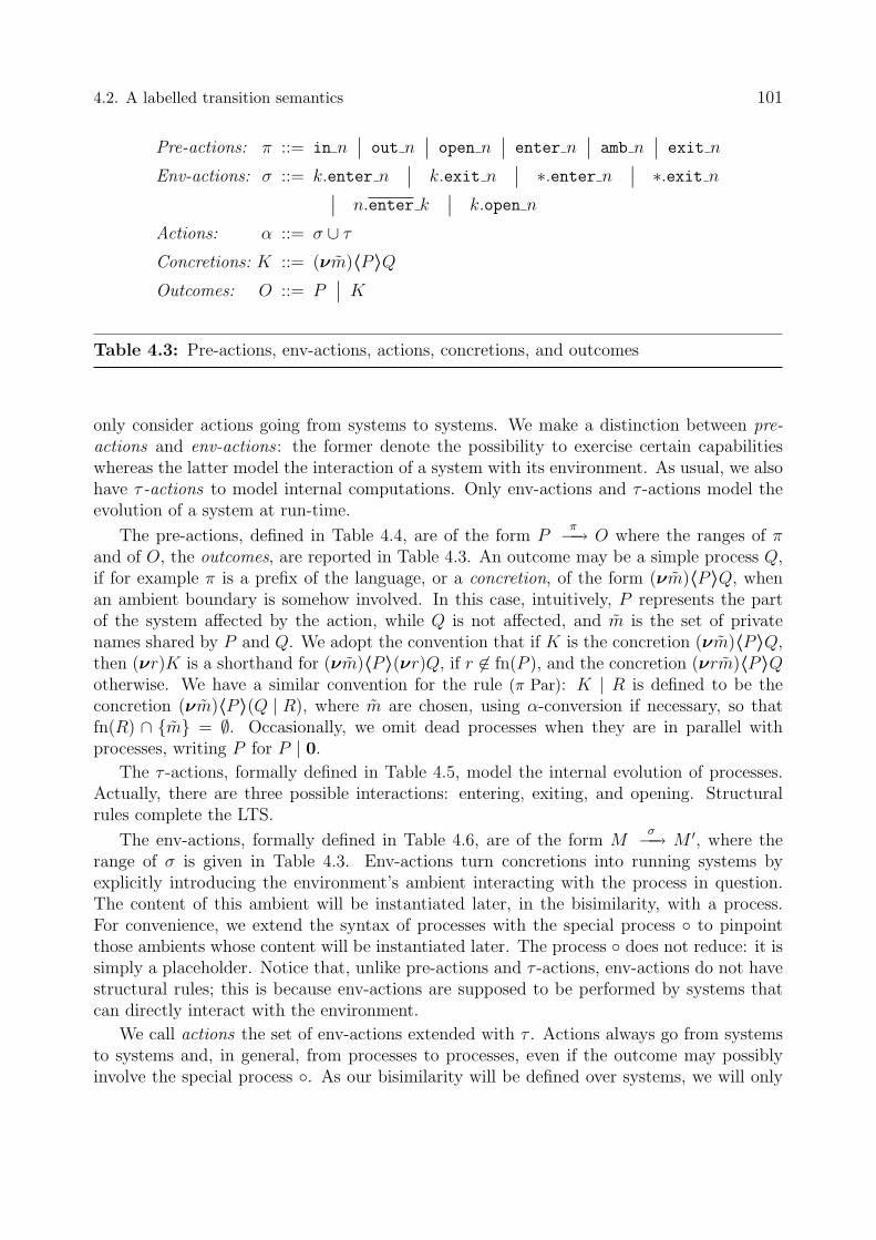
4.2. A labelled transition semantics 101

Pre-actions: π ::= in n∣∣ out n

∣∣ open n∣∣ enter n

∣∣ amb n∣∣ exit n

Env-actions: σ ::= k.enter n∣∣ k.exit n

∣∣ ∗.enter n∣∣ ∗.exit n∣∣ n.enter k

∣∣ k.open n

Actions: α ::= σ ∪ τ

Concretions: K ::= (νm)〈P 〉QOutcomes: O ::= P

∣∣ K

Table 4.3: Pre-actions, env-actions, actions, concretions, and outcomes

only consider actions going from systems to systems. We make a distinction between pre-actions and env-actions : the former denote the possibility to exercise certain capabilitieswhereas the latter model the interaction of a system with its environment. As usual, we alsohave τ -actions to model internal computations. Only env-actions and τ -actions model theevolution of a system at run-time.

The pre-actions, defined in Table 4.4, are of the form Pπ−−→ O where the ranges of π

and of O, the outcomes, are reported in Table 4.3. An outcome may be a simple process Q,if for example π is a prefix of the language, or a concretion, of the form (νm)〈P 〉Q, whenan ambient boundary is somehow involved. In this case, intuitively, P represents the partof the system affected by the action, while Q is not affected, and m is the set of privatenames shared by P and Q. We adopt the convention that if K is the concretion (νm)〈P 〉Q,then (νr)K is a shorthand for (νm)〈P 〉(νr)Q, if r 6∈ fn(P ), and the concretion (νrm)〈P 〉Qotherwise. We have a similar convention for the rule (π Par): K | R is defined to be theconcretion (νm)〈P 〉(Q | R), where m are chosen, using α-conversion if necessary, so thatfn(R) ∩ {m} = ∅. Occasionally, we omit dead processes when they are in parallel withprocesses, writing P for P | 0.

The τ -actions, formally defined in Table 4.5, model the internal evolution of processes.Actually, there are three possible interactions: entering, exiting, and opening. Structuralrules complete the LTS.

The env-actions, formally defined in Table 4.6, are of the form Mσ−−→ M ′, where the

range of σ is given in Table 4.3. Env-actions turn concretions into running systems byexplicitly introducing the environment’s ambient interacting with the process in question.The content of this ambient will be instantiated later, in the bisimilarity, with a process.For convenience, we extend the syntax of processes with the special process ◦ to pinpointthose ambients whose content will be instantiated later. The process ◦ does not reduce: it issimply a placeholder. Notice that, unlike pre-actions and τ -actions, env-actions do not havestructural rules; this is because env-actions are supposed to be performed by systems thatcan directly interact with the environment.

We call actions the set of env-actions extended with τ . Actions always go from systemsto systems and, in general, from processes to processes, even if the outcome may possiblyinvolve the special process ◦. As our bisimilarity will be defined over systems, we will only

102 Mobile Ambients

(π Pfx)π.P

π−−→ P(π Repl Pfx)

!π.Pπ−−→ P | !π.P

(π Enter)P

in n−−−−→ P1

m[P ]enter n−−−−−−→ 〈m[P1]〉0

(π Amb)n[P ]

amb n−−−−−→ 〈P 〉0

(π Exit)P

out n−−−−−→ P1

m[P ]exit n−−−−−→ 〈m[P1]〉0

(π Res)P

π−−→ O n 6∈ fn(π)

(νn)Pπ−−→ (νn)O

(π Par)P

π−−→ O

P | Q π−−→ O | QQ | P π−−→ Q | O

Table 4.4: Labelled transition system: pre-actions

(τ Enter)P

enter n−−−−−−→ (νp)〈P1〉P2 Qamb n−−−−−→ (ν q)〈Q1〉Q2

(∗)

P | Q τ−−→ (νp)(ν q)(n[P1 | Q1] | P2 | Q2)

Q | P τ−−→ (ν q)(νp)(n[Q1 | P1] | Q2 | P2)

(τ Exit)P

exit n−−−−−→ (νm)〈k[P1]〉P2

n[P ]τ−−→ (νm)(k[P1] | n[P2])

(τ Amb)P

τ−−→ Q

n[P ]τ−−→ n[Q]

(τ Open)P

open n−−−−−→ P1 Q

amb n−−−−−→ (νm)〈Q1〉Q2

P | Q τ−−→ P1 | (νm)(Q1 | Q2)

Q | P τ−−→ (νm)(Q1 | Q2) | P1

(τ Res)P

τ−−→ P ′

(νn)Pτ−−→ (νn)P ′

(τ Par)P

τ−−→ P ′

P | Q τ−−→ P ′ | QQ | P τ−−→ Q | P ′

(*) In rule (τ Enter) we require ((fn(P1) ∪ fn(P2)) ∩ {q}) = ((fn(Q1) ∪ fn(Q2)) ∩ {p}) = ∅.

Table 4.5: Labelled transition system: τ -actions

consider actions (and not pre-actions) in its definition.

Proposition 4.2.1 If T is a system (resp. a process), and Tα−−→ T ′, then T ′ is a system

(resp. a process), possibly containing the special process ◦.

We explain the rules induced by the the prefix in, the immigration of ambients. A typical

4.2. A labelled transition semantics 103

(Enter)

Penter n−−−−−−→ (νm)〈k[P1]〉P2

(†)

Pk.enter n−−−−−−−→ (νm)(n[◦ | k[P1]] | P2)

(Exit)

Pexit n−−−−−→ (νm)〈k[P1]〉P2

(†)

Pk.exit n−−−−−−→ (νm)(k[P1] | n[ ◦ | P2])

(Co-Enter)

Pamb n−−−−−→ (νm)〈P1〉P2

(†)

Pn.enter k−−−−−−−→ (νm)(n[P1 | k[ ◦ ]] | P2)

(Open)

Pamb n−−−−−→ (νm)〈P1〉P 2

Pk.open n−−−−−−→ k[◦ | (νm)(P1 | P2)]

(Enter Shh)

Penter n−−−−−−→ (νm)〈k[P1]〉P2

(‡)

P∗.enter n−−−−−−−→ (νm)(n[◦ | k[P1]] | P2)

(Exit Shh)

Pexit n−−−−−→ (νm)〈k[P1]〉P2

(‡)

P∗.exit n−−−−−−→ (νm)(k[P1] | n[◦ | P2])

(†) In rules (Enter), (Co-Enter), and (Exit) we require k 6∈ m;

(‡) In rules (Enter Shh) and (Exit Shh) we require k 6= n and k ∈ m.

Table 4.6: Labelled transition system: env-actions

example of an ambient m migrating into an ambient n follows:

(νm)(m[ in n.P1 | P2 ] | M) | n[Q] _ (νm)(M | n[m[P1 | P2 ] | Q])

The driving force behind the migration is the activation of the prefix in n, within the ambientm. It induces a capability in the ambient m to migrate into n, that we formalise as a newaction enter n. Thus an application of (π Enter) gives

m[in n.P1 | P2]enter n−−−−−−→ 〈m[P1 | P2]〉0

and more generally, using the structural rules (π Res) and (π Par),

(νm)(m[in n.P1 | P2] | M)enter n−−−−−−→ (νm)〈m[P1 | P2]〉M.

This means that the ambient m[in n.P1 | P2] has the capability to enter an ambient n; ifthe capability is exercised, the ambient m[P1 | P2] will enter n while M will be the residualwhere execution started. Of course the action can only be executed if there is an ambient nin parallel. The rule (π Amb) allows to check for the presence of ambients. So for example,we have

n[Q]amb n−−−−−→ 〈Q〉0.

Here, the concretion 〈Q〉0 says that Q is in n, while 0 is outside. Finally, the communication(τ Enter) allows these two complementary actions to occur simultaneously, executing themigration of the ambient m[P1 | P2] from its current computation space into the ambient n,giving rise to the original move above:

(νm)(m[ in n.P1 | P2 ] | M) | n[Q]τ−−→ (νm)(M | n[m[P1 | P2 ] | Q]).

104 Mobile Ambients

Note that this is a higher-order interaction, as the ambient m[P1 | P2] is transferred betweentwo computation spaces.

We have not said yet what env-actions are useful for. They model the interaction ofmobile agents with their environment. So, for instance, using the rule (Enter Shh), we derivefrom

(νm)(m[in n.P1 | P2] | M)enter n−−−−−−→ (νm)〈m[P1 | P2]〉M.

the transition

(νm)(m[in n.P1 | P2] | M)∗.enter n−−−−−−−→ (νm)(n[◦ | m[P1 | P2]] |M).

This transition denotes a private (secret) ambient entering an ambient n provided by theenvironment. The computation running at n can be added later by instantiating the place-holder ◦.

Had the ambient name m not been restricted, we would have used the rule (Enter) toderive

m[in n.P1 | P2] | Mm.enter n−−−−−−−−→ n[◦ | m[P1 | P2]] |M

to model a global ambient m that enters an ambient n provided by the environment.

The rule for emigration follows the same line. A typical example of ambient m emigratingfrom ambient n is as follows:

n[m[out n.P1 | P2] | Q] _ n[Q] | m[P1 | P2].

The driving force behind the emigration is the activation of the prefix out n within theambient m. It induces a capability in the ambient m to emigrate from n, which we formaliseas a new action exit n. Thus an application of the rule (π Exit), followed by (π Par), gives

m[out n.P1 | P2] | Qexit n−−−−−→ 〈m[P1 | P2]〉Q.

Here when this capability is exercised the code Q will remain inside the ambient n while theambient m[P1 | P2] will move outside. However to actually effect the emigration of m weneed a further context, namely the ambient n from which to emigrate. This leads to the rule(τ Exit); an application of which gives the original move above:

n[m[out n.P1 | P2] | Q]τ−−→ n[Q] | m[P1 | P2].

Again, env-actions can model the exiting of both private and global ambients from an ambientprovided by the environment.

Whenever a system offers a public ambient n at top-level, a context can interact with thesystem by providing an ambient entering n. The rule (Co-Enter) captures this interactionbetween system and environment. The rule that controls the opening follows along the samelines.

We end this section with a theorem that asserts that the LTS-based semantics coincideswith the reduction semantics of Section 4.1.

For any process P , outcome O and pre-action π such that Pπ−−→ O, the structure of

P and O can be determined up to structural congruence. We write O ≡ (ν r)〈P 〉Q as ashorthand for O = (ν r)〈P ′〉Q′ with P ≡ P ′ and Q ≡ Q′.

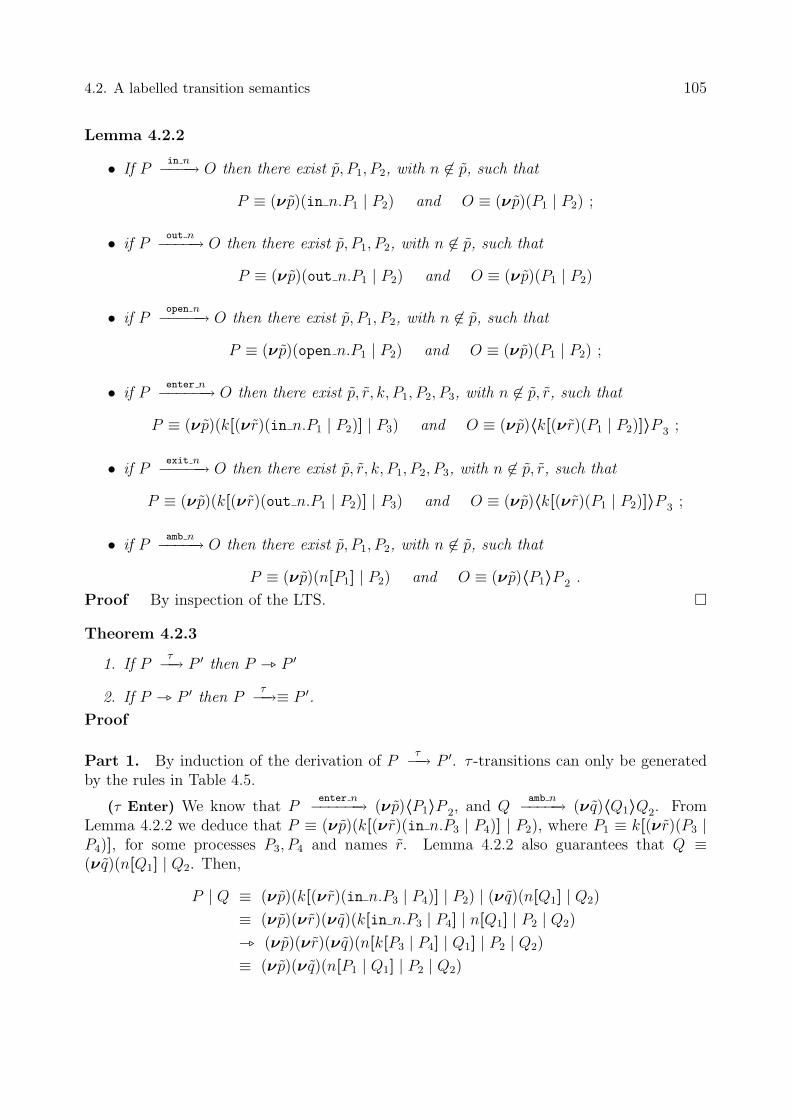
4.2. A labelled transition semantics 105

Lemma 4.2.2

• If Pin n−−−−→ O then there exist p, P1, P2, with n 6∈ p, such that

P ≡ (νp)(in n.P1 | P2) and O ≡ (νp)(P1 | P2) ;

• if Pout n−−−−−→ O then there exist p, P1, P2, with n 6∈ p, such that

P ≡ (νp)(out n.P1 | P2) and O ≡ (νp)(P1 | P2)

• if Popen n−−−−−→ O then there exist p, P1, P2, with n 6∈ p, such that

P ≡ (νp)(open n.P1 | P2) and O ≡ (νp)(P1 | P2) ;

• if Penter n−−−−−−→ O then there exist p, r, k, P1, P2, P3, with n 6∈ p, r, such that

P ≡ (νp)(k[(ν r)(in n.P1 | P2)] | P3) and O ≡ (νp)〈k[(ν r)(P1 | P2)]〉P 3 ;

• if Pexit n−−−−−→ O then there exist p, r, k, P1, P2, P3, with n 6∈ p, r, such that

P ≡ (νp)(k[(ν r)(out n.P1 | P2)] | P3) and O ≡ (νp)〈k[(ν r)(P1 | P2)]〉P 3 ;

• if Pamb n−−−−−→ O then there exist p, P1, P2, with n 6∈ p, such that

P ≡ (νp)(n[P1] | P2) and O ≡ (νp)〈P1〉P 2 .

Proof By inspection of the LTS. �

Theorem 4.2.3

1. If Pτ−−→ P ′ then P _ P ′

2. If P _ P ′ then Pτ−−→≡ P ′.

Proof

Part 1. By induction of the derivation of Pτ−−→ P ′. τ -transitions can only be generated

by the rules in Table 4.5.

(τ Enter) We know that Penter n−−−−−−→ (νp)〈P1〉P 2, and Q

amb n−−−−−→ (ν q)〈Q1〉Q2. FromLemma 4.2.2 we deduce that P ≡ (νp)(k[(ν r)(in n.P3 | P4)] | P2), where P1 ≡ k[(ν r)(P3 |P4)], for some processes P3, P4 and names r. Lemma 4.2.2 also guarantees that Q ≡(ν q)(n[Q1] | Q2. Then,

P | Q ≡ (νp)(k[(ν r)(in n.P3 | P4)] | P2) | (ν q)(n[Q1] | Q2)

≡ (νp)(ν r)(ν q)(k[in n.P3 | P4] | n[Q1] | P2 | Q2)

_ (νp)(ν r)(ν q)(n[k[P3 | P4] | Q1] | P2 | Q2)

≡ (νp)(ν q)(n[P1 | Q1] | P2 | Q2)

106 Mobile Ambients

as desired.

(τ Exit) We know that Pexit n−−−−−→ (νp)〈k[P1]〉P 2. From Lemma 4.2.2 we deduce that

P ≡ (νp)(k[(ν r)(out n.P3 | P4)] | P2), where P1 ≡ (ν r)(P3 | P4), for some processes P3, P4

and names r. Then,

n[P ] ≡ n[(νp)(k[(ν r)(out n.P3 | P4)] | P2)]

≡ (νp)(ν r)n[k[out n.P3 | P4] | P2)]

_ (νp)(ν r)(n[P2]k[P3 | P4])

≡ (νp)(n[P2]k[(ν r)(P3 | P4)])

as desired.

(τ Open) We know that Popen n−−−−−→ P1 and Q

amb n−−−−−→ (ν q)〈Q1〉Q2. From Lemma 4.2.2we deduce that P ≡ (νp)(open n.P2 | P3), where P1 ≡ (νp)(P2 | P3) for for some processesP2, P3. Lemma 4.2.2 also guarantees that Q ≡ (ν q)(n[Q1] | Q2). Then,

P | Q ≡ (νp)(open n.P2 | P3) | (ν q)(n[Q1] | Q2)

≡ (νp)(ν q)(open n.P2 | n[Q1] | P3 | Q2)

_ (νp)(ν q)(P2 | Q1 | P3 | Q2)

≡ (νp)(P2 | P3) | (ν q)(Q1 | Q2)

as desired.

The other cases follows straightforwardly from the congruence rules of the reductionrelation.

Part 2. By induction on the derivation of P _ Q. There are three base cases.

(Red In) We know that

n[in m.P | Q] | m[R] _ m[n[P | Q] | R] .

The derivation below is valid.

in m.Pin m−−−−→ P

in m.P | Q in m−−−−→ P | Q

n[in m.P | Q]enter m−−−−−−→ 〈P | Q〉0 m[R]

amb m−−−−−→ 〈R〉0

n[in m.P | Q] | m[R]τ−−→ m[n[P | Q] | R]

(Red Out) We know that

m[n[out m.P | Q] | R] _ n[P | Q] | m[R]

4.3. Characterising reduction barbed congruence 107

The derivation below is valid.

out m.Pout m−−−−−→ P

out m.P | Q out m−−−−−→ P | Q

n[out m.P | Q]exit m−−−−−−→ 〈n[P | Q]〉0

n[out m.P | Q] | R exit m−−−−−−→ 〈n[P | Q]〉R

m[n[out m.P | Q] | R]τ−−→ n[P | Q] | m[R]

(Red Open) We know that

open n.P | n[Q] _ P | Q

The derivation below is valid.

open n.Popen n−−−−−→ P n[Q]

amb n−−−−−→ 〈Q〉0

open n.P | n[Q]τ−−→ P | Q

The induction step, rule (Red Struct), follows because τ -transitions are preserved by allstatic contexts. �

Since we are interested in weak bisimilarities, that abstract over τ -actions, we introducethe notion of weak action. The definition is standard: =⇒ denotes the reflexive and transitiveclosure of

τ−−→;α

==⇒ denotes =⇒ α−−→ =⇒;α

==⇒ denotes =⇒ if α = τ andα

==⇒ otherwise.

Corollary 4.2.4 If M ≡ N and Mτ−−→ M ′, then there is N ′ such that N

τ−−→ N ′ andM ′ ≡ N ′.

From the results above, it is easy to establish that if M ∼= N then

• M ⇓ n iff N ⇓ n

• M =⇒M ′ implies there is N ′ such that N =⇒ N ′ and M ′ ∼= N ′.

In the sequel we will use these properties without comment.

4.3 Characterising reduction barbed congruence

In this section we define a labelled bisimilarity for MA that completely characterises reductionbarbed congruence.

In the previous section we said that actions (and more precisely env-actions) introduce aspecial process ◦ to pinpoint those ambients whose content will be specified in the bisimilarity.The • operator instantiates the placeholder with a process, as defined below. It performsa name-capture avoiding substitution. It should be pointed out that we allow structuralcongruence to rearrange terms containing ◦: with respect to structural congruence, ◦ behaveslike the inactive process 0. This motivates the introduction of the special process ◦, insteadof relying on standard process substitutions.

108 Mobile Ambients

Definition 4.3.1 Let T , T1, and T2 range over both systems and processes. Then, given aprocess P , we define:

0 • Pdef= 0 (T1 | T2) • P

def= (T1 • P ) | (T2 • P )

n[R] • Pdef= n[R • P ] (νn)T • P

def= (νn)(T • P ) if n 6∈ fn(P )

◦ • Pdef= P C.R • P

def= C.(R • P )

!C.R • Pdef= !C.(R • P ).

Everything is in place to define our bisimilarity.

Definition 4.3.2 (Late bisimilarity) A symmetric relation R between systems is a latebisimulation if M R N implies:

- if Mα−−→M ′, α 6∈ {∗.enter n, ∗.exit n}, then there is a system N ′ such that N

α==⇒

N ′ and for all processes P it holds M ′ • P R N ′ • P ;

- if M∗.enter n−−−−−−−→ M ′ then there is a system N ′ such that N | n[ ◦ ] =⇒ N ′ and for all

processes P it holds M ′ • P R N ′ • P ;

- if M∗.exit n−−−−−−→ M ′ then there is a system N ′ such that n[◦ | N ] =⇒ N ′ and for all

processes P it holds M ′ • P R N ′ • P .

Systems M and N are late bisimilar, written M ≈ N , if M R N for some late bisimulationR.

The bisimilarity above has a universal quantification over the process P provided by theenvironment. This process instantiates the special process ◦ generated via env-actions. Thebisimilarity is defined in a late style as the existential quantification precedes the universalone. Another possibility would be to define the bisimilarity in early style where the universalquantification over the environment’s contribution P precedes that over the derivative N ′.We write ≈e to denote this early variant. By definition, every late bisimulation is also a earlyone, while the converse, in general, does not hold. In our case, as in HOπ [San96a], we willprove that late and early bisimilarity actually coincide. As a consequence, late bisimilaritywill be our main labelled bisimilarity because the derivatives N ′ do not depend on processesP .

In the definition of bisimilarity, actions ∗.enter n and ∗.exit n are treated apart ask-ing for weaker matching requirements. This is because both actions are not observable.Somehow, this is very similar to what happens with input actions in the asynchronous π-calculus [HT91, Bou92].

Finally, the π-calculus experience suggests that late bisimulations like the one we definedmight fail to be transitive. As we will see, processes reveal to be more ‘tractable’ than names,and in our framework late bisimilarity turns out to be an equivalence relation.

4.3. Characterising reduction barbed congruence 109

4.3.1 Soundness

Late and early bisimilarity represent two proof techniques for reduction barbed congruence.More precisely we prove that they are both contextual and contained in reduction barbedcongruence.

The following lemma is crucial for proving that ≈ is contextual. This lemma will be alsoused for proving the soundness of the up-to context proof techniques in Section 4.4.

Lemma 4.3.3 Let S be a contextual symmetric relation between systems. Let (M, N) ∈ Sbe a pair satisfying the bisimulation conditions in S, that is,

- if Mα−−→M ′, α 6∈ {∗.enter n, ∗.exit n}, then there is a system N ′ such that N

α==⇒

N ′ and for all processes P it holds M ′ • P S N ′ • P ;

- if M∗.enter n−−−−−−−→ M ′ then there is a system N ′ such that N | n[ ◦ ] =⇒ N ′ and for all

processes P it holds M ′ • P S N ′ • P ;

- if M∗.exit n−−−−−−→ M ′ then there is a system N ′ such that n[◦ | N ] =⇒ N ′ and for all

processes P it holds M ′ • P S N ′ • P .

Then, for any system context C[−], all the pairs (C[M ], C[N ]) also satisfy the bisimulationconditions in S.Proof The relation S is contextual, and as such it is the smallest relation between systemssuch that:

- if M S N , then M | H S N | H and H |M S H | N for all systems H;

- if M S N , then (νm)M S (νm)N for all names m;

- if M S N , then m[M | P ] S m[N | P ] and m[P |M ] S m[P | N ] for all names m andprocesses P .

We prove the closure of C[M ] S C[N ] under the conditions for being a bisimulation byinduction on the structure of C[−] (we will not discuss the symmetric cases: they followaccordingly).

• C[−] = −.

This case holds because M S N satisfies the bisimulation conditions in S.

• C[−] = (νm)D[−].

We know that D[M ] S D[N ] satisfies the bisimulation conditions in S, and we want toprove that (νm)D[M ] S (νm)D[N ] satisfies the bisimulation conditions in S as well.

Suppose (νm)D[M ]α−−→. We perform a case analysis on α.

– (νm)D[M ]τ−−→ O1.

This can only be derived from D[M ]τ−−→ O1, where O1 = (νm)O1. The induction

hypothesis tells us that there exists a system O2 such that D[N ] =⇒ O2 andO1 S O2. We can derive (νm)D[N ] =⇒ (νm)O2 and conclude (νm)O1 S (νm)O2

because S is closed under restriction.

110 Mobile Ambients

– (νm)D[M ]k.enter n−−−−−−−→ O1.

Observe that this must have been derived from

D[M ]enter n−−−−−−→ (ν r)〈k[M1]〉M2

(νm)D[M ]enter n−−−−−−→ (νm)(ν r)〈k[M1]〉M2

(νm)D[M ]k.enter n−−−−−−−→ O1 ≡ (νm)(ν r)(n[◦ | k[M1]] |M2)

for some process M1 and system M2. Remark that this implies m 6= n and

m 6= k. As D[M ]enter n−−−−−−→ (ν r)〈k[M1]〉M2 then D[M ]

k.enter n−−−−−−−→ (ν r)(n[◦ |k[M1]] | M2) = M ′. The induction hypothesis then tells us that there exist

systems N ′, A,B such that D[N ] =⇒ Ak.enter n−−−−−−−→ B =⇒ N ′, and for all processes

P it holds M ′ • P S N ′ • P . As Ak.enter n−−−−−−−→ B, the system B must be of the

form (νs)(n[◦ | k[N1]] | N2), for some process N1 and system N2. It also holds

Aenter n−−−−−−→ (νs)〈k[N1]〉N2. This implies (νm)A

enter n−−−−−−→ (νm)(νs)〈k[N1]〉N2,

from which we can derive (νm)Ak.enter n−−−−−−−→ C ≡ (νm)B = (νm)(νs)(n[◦ |

k[N1]] | N2). We obtain (νm)D[N ] =⇒ (νm)Ak.enter n−−−−−−−→ C =⇒≡ (νm)N ′. Call

(νm)N ′ = O2. We can conclude that for all processes P , it holds O1 •P S O2 •Pup to structural congruence, because S is closed under restriction.

– (νm)D[M ]k.exit n−−−−−−→ O1.

Observe that this must have been derived from

D[M ]exit n−−−−−→ (ν r)〈k[M1]〉M2

(νm)D[M ]exit n−−−−−→ (νm)(ν r)〈k[M1]〉M2

(νm)D[M ]k.exit n−−−−−−→ O1 ≡ (νm)(ν r)(n[◦ |M2] | k[M1])

for some process M1 and system M2. Remark that this implies m 6= n and

m 6= k. As D[M ]exit n−−−−−→ (ν r)〈k[M1]〉M2 then D[M ]

k.exit n−−−−−−→ (ν r)(n[◦ |M2] | k[M1]) = M ′. The induction hypothesis then tells us that there exist

systems N ′, A,B such that D[N ] =⇒ Ak.exit n−−−−−−→ B =⇒ N ′, and for all processes

P it holds M ′ • P S N ′ • P . As Ak.exit n−−−−−−→ B, the system B must be of the

form (νs)(n[◦ | N2] | k[N1]), for some process N1 and system N2. It also holds

Aexit n−−−−−→ (νs)〈k[N1]〉N2. This implies (νm)A

exit n−−−−−→ (νm)(νs)〈k[N1]〉N2,

from which we can derive (νm)Ak.exit n−−−−−−→ C ≡ (νm)B = (νm)(νs)(n[◦ |

N2] | k[N1]). We obtain (νm)D[N ] =⇒ (νm)Ak.exit n−−−−−−→ C =⇒≡ (νm)N ′. Call

(νm)N ′ = O2. We can conclude that for all processes P , it holds O1 •P S O2 •Pup to structural congruence, because S is closed under restriction.

– (νm)D[M ]n.enter k−−−−−−−→ O1.

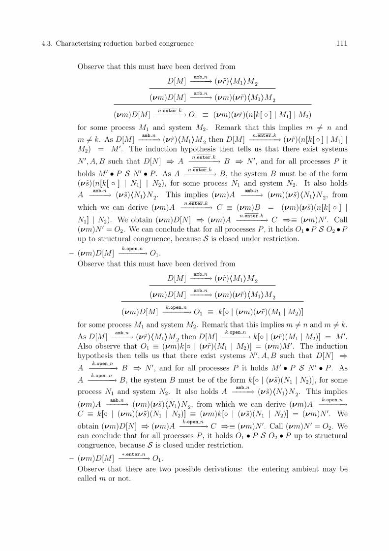
4.3. Characterising reduction barbed congruence 111

Observe that this must have been derived from

D[M ]amb n−−−−−→ (ν r)〈M1〉M2

(νm)D[M ]amb n−−−−−→ (νm)(ν r)〈M1〉M2

(νm)D[M ]n.enter k−−−−−−−→ O1 ≡ (νm)(ν r)(n[k[ ◦ ] |M1] |M2)

for some process M1 and system M2. Remark that this implies m 6= n and

m 6= k. As D[M ]amb n−−−−−→ (ν r)〈M1〉M2 then D[M ]

n.enter k−−−−−−−→ (ν r)(n[k[ ◦ ] |M1] |M2) = M ′. The induction hypothesis then tells us that there exist systems

N ′, A,B such that D[N ] =⇒ An.enter k−−−−−−−→ B =⇒ N ′, and for all processes P it

holds M ′ • P S N ′ • P . As An.enter k−−−−−−−→ B, the system B must be of the form

(νs)(n[k[ ◦ ] | N1] | N2), for some process N1 and system N2. It also holds

Aamb n−−−−−→ (νs)〈N1〉N2. This implies (νm)A

amb n−−−−−→ (νm)(νs)〈N1〉N2, from

which we can derive (νm)An.enter k−−−−−−−→ C ≡ (νm)B = (νm)(νs)(n[k[ ◦ ] |

N1] | N2). We obtain (νm)D[N ] =⇒ (νm)An.enter k−−−−−−−→ C =⇒≡ (νm)N ′. Call

(νm)N ′ = O2. We can conclude that for all processes P , it holds O1 •P S O2 •Pup to structural congruence, because S is closed under restriction.

– (νm)D[M ]k.open n−−−−−−→ O1.

Observe that this must have been derived from

D[M ]amb n−−−−−→ (ν r)〈M1〉M2

(νm)D[M ]amb n−−−−−→ (νm)(ν r)〈M1〉M2

(νm)D[M ]k.open n−−−−−−→ O1 ≡ k[◦ | (νm)(ν r)(M1 |M2)]

for some process M1 and system M2. Remark that this implies m 6= n and m 6= k.

As D[M ]amb n−−−−−→ (ν r)〈M1〉M2 then D[M ]

k.open n−−−−−−→ k[◦ | (ν r)(M1 |M2)] = M ′.

Also observe that O1 ≡ (νm)k[◦ | (ν r)(M1 | M2)] = (νm)M ′. The inductionhypothesis then tells us that there exist systems N ′, A,B such that D[N ] =⇒A

k.open n−−−−−−→ B =⇒ N ′, and for all processes P it holds M ′ • P S N ′ • P . As

Ak.open n−−−−−−→ B, the system B must be of the form k[◦ | (νs)(N1 | N2)], for some

process N1 and system N2. It also holds Aamb n−−−−−→ (νs)〈N1〉N2. This implies

(νm)Aamb n−−−−−→ (νm)(νs)〈N1〉N2, from which we can derive (νm)A

k.open n−−−−−−→

C ≡ k[◦ | (νm)(νs)(N1 | N2)] ≡ (νm)k[◦ | (νs)(N1 | N2)] = (νm)N ′. We

obtain (νm)D[N ] =⇒ (νm)Ak.open n−−−−−−→ C =⇒≡ (νm)N ′. Call (νm)N ′ = O2. We

can conclude that for all processes P , it holds O1 • P S O2 • P up to structuralcongruence, because S is closed under restriction.

– (νm)D[M ]∗.enter n−−−−−−−→ O1.

Observe that there are two possible derivations: the entering ambient may becalled m or not.

112 Mobile Ambients

∗ Suppose:

D[M ]enter n−−−−−−→ (ν r)〈m[M1]〉M2

(νm)D[M ]enter n−−−−−−→ (νm)(ν r)〈m[M1]〉M2

(νm)D[M ]∗.enter n−−−−−−−→ O1 ≡ (νm)(ν r)(n[◦ | m[M1]] |M2)

where m 6∈ r, for some process M1 and system M2. Remark that this implies

n 6∈ r. As D[M ]enter n−−−−−−→ (ν r)〈m[M1]〉M2 then D[M ]

m.enter n−−−−−−−−→ (ν r)(n[◦ |m[M1]] | M2) = M ′. The induction hypothesis then tells us that there

exist systems N ′, A,B such that D[N ] =⇒ Am.enter n−−−−−−−−→ B =⇒ N ′, and

for all processes P it holds M ′ • P S N ′ • P . As Am.enter n−−−−−−−−→ B, the

system B must be of the form (νs)(n[◦ | m[N1]] | N2), for some process

N1 and system N2, where m 6∈ s. It also holds Aenter n−−−−−−→ (νs)〈m[N1]〉N2.

This implies (νm)Aenter n−−−−−−→ (νm)(νs)〈m[N1]〉N2, from which we can derive

(νm)A | n[ ◦ ]τ−−→ C ≡ (νm)B = (νm)(νs)(n[◦ | N2] | m[N1]). We obtain

(νm)(D[N ] | n[ ◦ ]) ≡ (νm)D[N ] | n[ ◦ ] =⇒ (νm)A | n[ ◦ ]τ−−→ C =⇒≡

(νm)N ′. Call (νm)N ′ = O2. We can conclude that for all processes P , itholds O1 •P S O2 •P up to structural congruence, because S is closed underrestriction.

∗ Suppose:

D[M ]enter n−−−−−−→ (ν r)〈k[M1]〉M2

(νm)D[M ]enter n−−−−−−→ (νm)(ν r)〈k[M1]〉M2

(νm)D[M ]∗.enter n−−−−−−−→ O1 ≡ (νm)(ν r)(n[◦ | k[M1]] |M2)

where k 6= m and thus k ∈ r, for some process M1 and system M2. Remark

that n 6∈ r. Since D[M ]enter n−−−−−−→ (ν r)〈k[M1]〉M2, then D[M ]

∗.enter n−−−−−−−→(ν r)(n[◦ | k[M1]] | M2) = M ′. The induction hypothesis then tells us thatthere exists a system N ′ such that D[N ] | n[ ◦ ] =⇒ N ′, and for all processesP it holds M ′ •P S N ′ •P . We can derive (νm)D[N ] | n[ ◦ ] ≡ (νm)(D[N ] |n[◦]) =⇒ (νm)N ′. Call (νm)N ′ = O2. We can conclude that for all processesP , it holds O1 • P S O2 • P up to structural congruence, because S is closedunder restriction.

– (νm)D[M ]∗.exit n−−−−−−→ O1.

Observe that there are two possible derivations.

∗ Suppose:

D[M ]exit n−−−−−→ (ν r)〈m[M1]〉M2

(νm)D[M ]exit n−−−−−→ (νm)(ν r)〈m[M1]〉M2

(νm)D[M ]∗.exit n−−−−−−→ O1 ≡ (νm)(ν r)(n[◦ |M2] | m[M1])

4.3. Characterising reduction barbed congruence 113

where m 6∈ r, for some process M1 and system M2. Remark that this implies

n 6∈ r. As D[M ]exit n−−−−−→ (ν r)〈m[M1]〉M2 then D[M ]

m.exit n−−−−−−−→ (ν r)(n[◦ |M2] | m[M1]) = M ′. The induction hypothesis then tells us that there exist

systems N ′, A,B such that D[N ] =⇒ Am.exit n−−−−−−−→ B =⇒ N ′, and for all

processes P it holds M ′ • P S N ′ • P . As Am.exit n−−−−−−−→ B, the system B

must be of the form (νs)(n[◦ | N2] | m[N1]), for some process N1 and system

N2, where m 6∈ s. It also holds Aexit n−−−−−→ (νs)〈k[N1]〉N2. This implies

(νm)Aexit n−−−−−→ (νm)(νs)〈m[N1]〉N2, from which we can derive (νm)n[◦ |

A]τ−−→ C ≡ (νm)B = (νm)(νs)(n[◦ | N2] | m[N1]). We obtain (νm)(D[N ] |

n[ ◦ ]) ≡ (νm)D[N ] | n[ ◦ ] =⇒ (νm)A | n[ ◦ ]τ−−→ C =⇒≡ (νm)N ′. Call

(νm)N ′ = O2. We can conclude that for all processes P , it holds O1 • P SO2 • P up to structural congruence, because S is closed under restriction.

∗ Suppose:

D[M ]exit n−−−−−→ (ν r)〈k[M1]〉M2

(νm)D[M ]exit n−−−−−→ (νm)(ν r)〈k[M1]〉M2

(νm)D[M ]∗.exit n−−−−−−→ O1 ≡ (νm)(ν r)(n[◦ |M2] | k[M1])

where k 6= m and thus k ∈ r, for some process M1 and system M2. Remark

that n 6∈ r. Since D[M ]exit n−−−−−→ (ν r)〈k[M1]〉M2, then D[M ]

∗.exit n−−−−−−→(ν r)(n[◦ | M2] | k[M1]) = M ′. The induction hypothesis then tells us thatthere exists a system N ′ such that n[◦ | D[N ]] =⇒ N ′, and for all processes Pit holds M ′ • P S N ′ • P . We can derive (νm)D[N ] | n[ ◦ ] ≡ (νm)(D[N ] |n[◦]) =⇒ (νm)N ′. Call (νm)N ′ = O2. We can conclude that for all processesP , it holds O1 • P S O2 • P up to structural congruence, because S is closedunder restriction.

• C[−] = D[−] | H.

We know that D[M ] S D[N ] satisfies the bisimulation conditions in S, and we wantto prove that D[M ] | H S D[N ] | H satisfies the bisimulation conditions in S as well.

We perform a case analysis on the transition D[M ] | H α−−→ O1.

We consider first the cases when there is no interaction between D[M ] and H.

– D[M ] | Hτ−−→ O1, because D[M ]

τ−−→ M ′ and O1 ≡ M ′ | H. The inductionhypothesis tells us that there exists a N ′ such that D[N ] =⇒ N ′ and M ′ S N ′.Thus, D[N ] | H =⇒ O2 ≡ N ′ | H and O1 ≡ M ′ | H S N ′ | H ≡ O2 because S isclosed under parallel composition.

– D[M ] | H τ−−→ O1, because Hτ−−→ H ′ and O1 ≡ D[M ] | H ′. Let O2 = D[N ] | H ′:

it holds D[N ] | H τ−−→ O2, and O1 S O2 because D[M ] S D[N ] and S is closedunder parallel composition.

114 Mobile Ambients

– D[M ] | H k.enter n−−−−−−−→ O1.

There are two possible derivations.

∗ Suppose:

D[M ]enter n−−−−−−→ (ν r)〈k[M1]〉M2

D[M ] | H enter n−−−−−−→ (ν r)〈k[M1]〉M2 | H

D[M ] | H k.enter n−−−−−−−→ O1 ≡ (ν r)(n[◦ | k[M1]] |M2 | H)

for some process M1 and system M2. Remark that k 6∈ r. As D[M ]enter n−−−−−−→

(ν r)〈k[M1]〉M2 then D[M ]k.enter n−−−−−−−→ (ν r)(n[◦ | k[M1]] | M2) = M ′. The

induction hypothesis then tells us that there exist systems N ′, A,B such that

D[N ] =⇒ Ak.enter n−−−−−−−→ B =⇒ N ′, and for all processes P it holds M ′ • P S

N ′ • P . As Ak.enter n−−−−−−−→ B, the system B must be of the form (νs)(n[◦ |

k[N1]] | N2), for some process N1 and system N2. It also holds Aenter n−−−−−−→

(νs)〈k[N1]〉N2. This implies A | Henter n−−−−−−→ (νs)〈k[N1]〉N2 | H, from

which we can derive A | H k.enter n−−−−−−−→ (νs)(n[◦ | k[N1]] | N2 | H) ≡ B | H.

We obtain D[N ] | H =⇒ A | Hk.enter n−−−−−−−→≡ B | H =⇒≡ N ′ | H. Call

N ′ | H = O2. We can conclude that for all processes P , it holds O1•P S O2•Pup to structural congruence, because S is closed under parallel composition.

∗ Suppose:

Henter n−−−−−−→ (ν r)〈k[H1]〉H2

D[M ] | H enter n−−−−−−→ (ν r)〈k[H1]〉H2 | D[M ]

D[M ] | H k.enter n−−−−−−−→ O1 ≡ (ν r)(n[◦ | k[H1]] | H2 |M)

for some process H1 and system H2. Remark that k 6∈ r. We can constructthe following derivation:

Henter n−−−−−−→ (ν r)〈k[H1]〉H2

D[N ] | H enter n−−−−−−→ (ν r)〈k[H1]〉H2 | D[N ]

D[N ] | H k.enter n−−−−−−−→ (ν r)(n[◦ | k[H1]] | H2 | D[N ]) = O2

We can conclude that for all processes P , it holds O1 • P S O2 • P up tostructural congruence, because D[M ] S D[N ] and S is closed under parallelcomposition.

– D[M ] | H k.exit n−−−−−−→ O1.

There are two possible derivations.

4.3. Characterising reduction barbed congruence 115

∗ Suppose:

D[M ]exit n−−−−−→ (ν r)〈k[M1]〉M2

D[M ] | H exit n−−−−−→ (ν r)〈k[M1]〉M2 | H

D[M ] | H k.exit n−−−−−−→ O1 ≡ (ν r)(n[◦ |M2 | H] | k[M1])

for some process M1 and system M2. Remark that k 6∈ r. As D[M ]exit n−−−−−→

(ν r)〈k[M1]〉M2 then D[M ]k.exit n−−−−−−→ (ν r)(n[◦ | M2] | k[M1]) = M ′. The

induction hypothesis then tells us that there exist systems N ′, A,B such that

D[N ] =⇒ Ak.exit n−−−−−−→ B =⇒ N ′, and for all processes P it holds M ′•P S N ′•

P . Remark that N ′ ≡ (νh)n[◦ | N3] | N4, for some N3, N4. As Ak.exit n−−−−−−→ B,

the system B must be of the form (νs)(n[◦ | N2] | k[N1]), for some process

N1 and system N2. It also holds Aexit n−−−−−→ (νs)〈k[N1]〉N2. This implies

A | H exit n−−−−−→ (νs)〈k[N1]〉N2 | H, from which we can derive A | H k.exit n−−−−−−→(νs)(n[◦ | N2 | H] | k[N1]) ≡ B • (◦ | H). We obtain D[N ] | H =⇒ A |H

k.exit n−−−−−−→ B • (◦ | H) =⇒≡ N ′ • (◦ | H). Call N ′ • (◦ | H) = O2. Asfor all processes P it holds M ′ • P S N ′ • P , we can conclude that for allprocesses Q, it holds O1 • Q S O2 • Q up to structural congruence, becauseO1 •Q ≡M ′ • (Q | H) S N ′ • (Q | H) ≡ O2 •Q.

∗ Suppose:

Hexit n−−−−−→ (ν r)〈k[H1]〉H2

D[M ] | H exit n−−−−−→ (ν r)〈k[H1]〉H2 | D[M ]

D[M ] | H k.exit n−−−−−−→ O1 ≡ (ν r)(n[◦ | H2 | D[M ]] | k[H1])

for some process H1 and system H2. Remark that k 6∈ r. We can constructthe following derivation:

Hexit n−−−−−→ (ν r)〈k[H1]〉H2

D[N ] | H exit n−−−−−→ (ν r)〈k[H1]〉H2 | D[N ]

D[N ] | H k.exit n−−−−−−→ (ν r)(n[◦ | H2 | D[N ]] | k[H1]) = O2

We can conclude that for all processes P , it holds O1 • P S O2 • P up tostructural congruence, because D[M ] S D[N ] and S is closed under parallelcomposition and ambient.

– D[M ] | H n.enter k−−−−−−−→ O1.

There are two possible derivations.

116 Mobile Ambients

∗ Suppose:

D[M ]amb n−−−−−→ (ν r)〈M1〉M2

D[M ] | H amb n−−−−−→ (ν r)〈M1〉M2 | H

D[M ] | H n.enter k−−−−−−−→ O1 ≡ (ν r)(n[k[ ◦ ] |M1] |M2 | H)

for some process M1 and system M2. Remark that k, n 6∈ r. As D[M ]amb n−−−−−→

(ν r)〈M1〉M2 then D[M ]n.enter k−−−−−−−→ (ν r)(n[k[ ◦ ] | M1] | M2) = M ′. The

induction hypothesis then tells us that there exist systems N ′, A,B such that

D[N ] =⇒ An.enter k−−−−−−−→ B =⇒ N ′, and for all processes P it holds M ′ • P S

N ′ • P . As An.enter k−−−−−−−→ B, the system B must be of the form (νs)(n[k[ ◦ ] |

N1] | N2), for some process N1 and system N2. It also holds Aamb n−−−−−→

(νs)〈N1〉N2. This implies A | Hamb n−−−−−→ (νs)〈N1〉N2 | H, from which we

can derive A | H n.enter k−−−−−−−→ (νs)(n[k[◦] | N1] | N2 | H) ≡ B | H. We obtain

D[N ] | H =⇒ A | Hn.enter k−−−−−−−→≡ B | H =⇒≡ N ′ | H. Call N ′ | H = O2.

We can conclude that for all processes P , it holds O1 • P S O2 • P up tostructural congruence, because S is closed under parallel composition.

∗ Suppose:

Hamb n−−−−−→ (ν r)〈H1〉H2

D[M ] | H amb n−−−−−→ (ν r)〈H1〉H2 | D[M ]

D[M ] | H n.enter k−−−−−−−→ O1 ≡ (ν r)(n[k[ ◦ ] | H1] | H2 | D[M ])

for some process H1 and system H2. Remark that k 6∈ r. We can constructthe following derivation:

Hamb n−−−−−→ (ν r)〈H1〉H2

D[N ] | H amb n−−−−−→ (ν r)〈H1〉H2 | D[N ]

D[N ] | H n.enter k−−−−−−−→ (ν r)(n[k[ ◦ ] | H1] | H2 | D[N ]) = O2

We can conclude that for all processes P , it holds O1 • P S O2 • P up tostructural congruence, because D[M ] S D[N ] and S is closed under parallelcomposition.

– D[M ] | Hk.open n−−−−−−→ O1.

There are two possible derivations.

4.3. Characterising reduction barbed congruence 117

∗ Suppose:

D[M ]amb n−−−−−→ (ν r)〈M1〉M2

D[M ] | H amb n−−−−−→ (ν r)〈M1〉M2 | H

D[M ] | Hk.open n−−−−−−→ O1 ≡ k[◦ | (ν r)(M1 |M2) | H]

for some process M1 and system M2. Remark that k, n 6∈ r. As D[M ]amb n−−−−−→

(ν r)〈M1〉M2 then D[M ]k.open n−−−−−−→ k[◦ | (ν r)(M1 | M2)]. The induction

hypothesis then tells us that there exist systems N ′, A,B such that D[N ] =⇒A

k.open n−−−−−−→ B =⇒ N ′, and for all processes P it holds M ′ • P S N ′ • P .

As Ak.open n−−−−−−→ B, the system B must be of the form k[◦ | (νs)(N1 | N2)],

for some process N1 and system N2. It also holds Aamb n−−−−−→ (νs)〈N1〉N2.

This implies A | Hamb n−−−−−→ (νs)〈N1〉N2 | H, from which we can derive

A | Hk.open n−−−−−−→ k[◦ | (νs)(N1 | N2) | H] ≡ B • (◦ | H). We obtain

D[N ] | H =⇒ A | Hk.open n−−−−−−→≡ B • (◦ | H) =⇒≡ N ′ • (◦ | H). Call

N ′ • (◦ | H) = O2. We can conclude that for all processes P , it holdsO1 • P S O2 • P up to structural congruence, because for all processes P itholds M ′ • (P | H) S N ′ • (P | H).

∗ Suppose:

Hamb n−−−−−→ (νh)〈H1〉H2

D[M ] | H amb n−−−−−→ (νh)〈H1〉H2 | D[M ]

D[M ] | Hk.open n−−−−−−→ O1 ≡ k[◦ | (νh)(H1 | H2) | D[M ]]

for some process H1 and system H2. Remark that k 6∈ h. We can constructthe following derivation:

Hamb n−−−−−→ (νh)〈H1〉H2

D[N ] | H amb n−−−−−→ (νh)〈H1〉H2 | D[N ]

D[N ] | Hk.open n−−−−−−→ k[◦ | (νh)(H1 | H2) | D[N ]] = O2

We can conclude that for all processes P , it holds O1 • P S O2 • P up tostructural congruence, because D[M ] S D[N ] and S is closed under parallelcomposition and ambient.

– D[M ] | H ∗.enter n−−−−−−−→ O1.

There are two possible derivations.

118 Mobile Ambients

∗ Suppose:

D[M ]enter n−−−−−−→ (ν r)〈k[M1]〉M2

D[M ] | H enter n−−−−−−→ (ν r)〈k[M1]〉M2 | H

D[M ] | H ∗.enter n−−−−−−−→ O1 ≡ (ν r)(n[◦ | k[M1]] |M2 | H)

where k ∈ r, for some process M1 and system M2. Remark that n 6∈ r. As

D[M ]enter n−−−−−−→ (ν r)〈k[M1]〉M2 then D[M ]

∗.enter n−−−−−−−→ (ν r)(n[◦ | k[M1]] |M2) = M ′. The induction hypothesis then tells us that there exist asystem N ′ such that D[N ] | n[ ◦ ] =⇒ N ′, and for all processes P it holdsM ′•P S N ′•P . We can derive D[N ] | n[◦] | H =⇒ N ′ | H. Call N ′ | H = O2.We can conclude that for all processes P , it holds O1 • P S O2 • P up tostructural congruence, because S is closed under parallel composition.

∗ Suppose:

Henter n−−−−−−→ (ν r)〈k[H1]〉H2

D[M ] | H enter n−−−−−−→ (ν r)〈k[H1]〉H2 | D[M ]

D[M ] | H ∗.enter n−−−−−−−→ O1 ≡ (ν r)(n[◦ | k[H1]] | H2 | D[M ])

where k ∈ r for some process H1 and system H2. We can construct thefollowing derivation:

Henter n−−−−−−→ (ν r)〈k[H1]〉H2

D[N ] | H enter n−−−−−−→ (ν r)〈k[H1]〉H2 | D[N ] n[ ◦ ]amb n−−−−−→ 〈 ◦ 〉0

D[N ] | H | n[ ◦ ]τ−−→ (ν r)(n[◦ | k[H1]] | H2 | D[N ]) = O2

We can conclude that for all processes P , it holds O1 • P S O2 • P up tostructural congruence, because D[M ] S D[N ] and S is closed under parallelcomposition.

– D[M ] | H ∗.exit n−−−−−−→ O1.

There are two possible derivations.

∗ Suppose:

D[M ]exit n−−−−−→ (ν r)〈k[M1]〉M2

D[M ] | H exit n−−−−−→ (ν r)〈k[M1]〉M2 | H

D[M ] | H ∗.exit n−−−−−−→ O1 ≡ (ν r)(n[◦ |M2 | H] | k[M1])

for some process M1 and system M2. Remark that k ∈ r. As D[M ]exit n−−−−−→

(ν r)〈k[M1]〉M2 then D[M ]∗.exit n−−−−−−→ (ν r)(n[◦ | M2] | k[M1]) = M ′. The

induction hypothesis then tells us that there exist systems N ′ such that n[◦ |

4.3. Characterising reduction barbed congruence 119

D[N ]] =⇒ N ′, and for all processes P it holds M ′ • P S N ′ • P . Remarkthat N ′ ≡ (νs)n[◦ | N3] | N4, for some N3, N4. We can derive n[ ◦ D[N ] |H] =⇒ (νs)n[◦ | N3 | H] | N4. Call (νs)n[◦ | N3 | H] | N4 = O2. Asfor all processes P it holds M ′ • P S N ′ • P , we can conclude that for allprocesses Q, it holds O1 • Q S O2 • Q up to structural congruence, becauseO1 •Q ≡M ′ • (Q | H) S N ′ • (Q | H) ≡ O2 •Q.

∗ Suppose:

Hexit n−−−−−→ (ν r)〈k[H1]〉H2

D[M ] | H exit n−−−−−→ (ν r)〈k[H1]〉H2 | D[M ]

D[M ] | H ∗.exit n−−−−−−→ O1 ≡ (ν r)(n[◦ | H2 | D[M ]] | k[H1])

for some process H1 and system H2. Remark that k ∈ r. We can constructthe following derivation:

Hexit n−−−−−→ (ν r)〈k[H1]〉H2

D[N ] | H exit n−−−−−→ (ν r)〈k[H1]〉H2 | D[N ]

n[◦ | D[N ] | H]τ−−→ (ν r)(n[◦ | H2 | D[N ]] | k[H1]) = O2

We can conclude that for all processes P , it holds O1 • P S O2 • P up tostructural congruence, because D[M ] S D[N ] and S is closed under parallelcomposition and ambient.

Then, we consider the cases when there is interaction between D[M ] and H.

– D[M ] | H τ−−→ O1, because

D[M ]enter n−−−−−−→ (νm)〈k[M1]〉M2 and H

amb n−−−−−→ (νh)〈H1〉H2.

Then O1 ≡ (νh, m)(n[k[M1] | H1] | M2 | H2). We distinguish the cases k ∈ m,and k 6∈ m.

∗ k 6∈ m. As D[M ]enter n−−−−−−→ (νm)〈k[M1]〉M2, it also holds D[M ]

k.enter n−−−−−−−→M ′ ≡ (νm)(n[◦ | k[M1]] | M2). The induction hypothesis tells us that there

exists a system N ′ such that D[N ]k.enter n

=======⇒ N ′ ≡ (νm)(n[◦ | k[N1]] | N2),

and for all processes P , it holds M ′ •P S N ′ •P . But if D[N ]k.enter n

=======⇒ N ′,

then D[N ]enter n

======⇒ (νm)〈k[N1]〉N2. This implies that D[N ] | H τ==⇒ O2 ≡

(νh, n)(n[k[N1] | H1] | N2 | H2). Since for all processes P , M ′ • P S N ′ • P ,it also holds M ′ • H1 S N ′ • H1, and O1 S O2 follows because S is closedunder parallel composition and restriction.

∗ k ∈ m. As D[M ]enter n−−−−−−→ (νm)〈k[M1]〉M2, it also holds D[M ]

enter n−−−−−−→M ′ ≡ (νm)(n[◦ | k[M1]] | M2). The induction hypothesis tells us that there

120 Mobile Ambients

exists a system N ′ such that D[N ] | n[ ◦ ] =⇒ N ′ ≡ (νn)(n[◦ | N1] | N2), andfor all processes P , it holds M ′ • P S N ′ • P . We can derive D[N ] | H =⇒O2 ≡ (νh, n)(n[N1 | H1] | N2 | H2). Since for all processes P , M ′•P S N ′•P ,it also holds M ′ • H1 S N ′ • H1, and O1 S O2 follows because S is closedunder parallel composition and restriction.

– D[M ] | H τ−−→ O1, because

D[M ]amb n−−−−−→ (νm)〈M1〉M2 and H

enter n−−−−−−→ (νh)〈k[H1]〉H2.

Then O1 ≡ (νh, m)(n[k[H1] | M1] | M2 | H2). As D[M ]amb n−−−−−→ (νm)〈M1〉M2,

it also holds D[M ]n.enter k−−−−−−−→ M ′ ≡ (νm)(n[k[ ◦ ] | M1] | M2). The induction

hypothesis tells us that there exists a system N ′ such that D[N ]n.enter k

=======⇒ N ′ ≡(νn)(n[k[ ◦ ] | N1] | N2), and for all processes P , it holds M ′ • P S N ′ • P .

As D[N ]n.enter k

=======⇒ N ′, we can derive D[N ]amb k

=====⇒ (νn)〈N1〉N2. It follows

D[N ] | H =⇒ (νh, n)(n[k[H1] | N1] | N2 | H2) = O2. Since for all processes P , itholds M ′ • P S N ′ • P , we have M ′ • h[H1] S N ′ • h[H1], and O1 S O2 followsbecause S is closed under parallel composition and restriction.

• C[−] = n[D[−] | P ], where P is an arbitrary process.

We know that D[M ] S D[N ] satisfies the bisimulation conditions in S, and we want toprove that n[D[M ] | P ] S n[D[N ] | P ] behaves as a bisimulation as well. We perform

a case analysis on the transition n[D[M ] | P ]α−−→ O1.

– n[D[M ] | P ]τ−−→ O1, because D[M ]

τ−−→ M ′. Then O1 ≡ n[M ′ | P ]. Theinduction hypothesis tells us that there exists a system N ′ such that D[N ] =⇒ N ′

and M ′ S N ′. We can derive n[D[N ] | P ] =⇒ n[N ′ | P ] and conclude n[M ′ | P ] Sn[N ′ | P ] because S is closed under ambient.

– n[D[M ] | P ]τ−−→ O1, because P

τ−−→ P ′. Then O1 ≡ n[D[M ] | P ′]. CallO2 = n[D[N ] | P ′]. Then O1 S O2 because D[M ] S D[N ], and S is closed underthe contexts of the form C[−] = n[− | Q] where Q is a process.

– n[D[M ] | P ]τ−−→ O1, because D[M ]

exit n−−−−−→ (ν r)〈k[M1]〉M2. Then O1 ≡(ν r)(k[M1] | n[M2 | P ]). We distinguish the two cases k ∈ r and k 6∈ r.

∗ k 6∈ r. From D[M ]exit n−−−−−→ (ν r)〈k[M1]〉M2 we can derive D[M ]

k.exit n−−−−−−→(ν r)(k[M1] | n[◦ |M2]). The induction hypothesis tells us that there exists a

system N ′ such that D[N ]k.exit n

=======⇒ N ′ ≡ (νs)(k[N1] | n[◦ | N2]) and for all

processes Q, it holds M ′ • Q S N ′ • Q. But D[N ]k.exit n

=======⇒ N ′ can only be

derived from D[N ]exit n

=====⇒ (νs)〈k[N1]〉N2 and thus n[D[N ] | P ] =⇒ N ′ • P .As for all processes Q, it holds M ′ •Q S N ′ •Q, we can derive (ν r)(k[M1] |n[P |M2]) S (νs)(k[N1] | n[P | N2]), as required.

4.3. Characterising reduction barbed congruence 121

∗ k ∈ r. From D[M ]exit n−−−−−→ (ν r)〈k[M1]〉M2 we can derive D[M ]

∗.exit n−−−−−−→(ν r)(k[M1] | n[◦ |M2]). The induction hypothesis tells us that there exists asystem N ′ such that n[◦ | D[N ]] =⇒ N ′ ≡ (νs)(k[N1] | n[◦ | N2]), and for allprocesses Q, it holds M ′ •Q S N ′ •Q. We can instantiate the placeholder ◦with the process P , thus obtaining the transition n[D[N ] | P ] =⇒ N ′ •P . Asfor all processes Q, it holds M ′ • Q S N ′ • Q , we have O1 = (νm)(k[M1] |n[P |M2]) ≡M ′ • P S N ′ • P ≡ (νs)(k[N1] | n[P | N2]) = O2, as required.

– n[D[M ] | P ]τ−−→ O1, because P

exit n−−−−−→ (ν r)〈k[P1]〉P 2. This implies O1 ≡(ν r)(k[P1] | n[D[M ] | P2]). It also holds n[D[N ] | P ]

τ−−→≡ (ν r)(k[P1] | n[D[N ] |P2]). Call this last term O2. The relation O1 S O2 follows because D[M ] S D[N ]and from the closure properties of S.

– n[D[M ] | P ]τ−−→ O1, and the τ action is generated by an interaction between

D[M ] and P . There are three cases.

∗ D[M ]amb m−−−−−→ (ν r)〈M1〉M2 and P

open m−−−−−−→ P ′. Then O1 = n[(ν r)(M1 |

M2) | P ′]. It holds D[M ]n.open m−−−−−−−→ n[◦ | (ν r)(M1 | M2)]. The induction

hypothesis tells us that there exists a system N ′ such that D[N ]n.open m−−−−−−−→ N ′,

and for all processes Q it holds M ′ • Q S N ′ • Q. The system N ′ mustbe of the form n[◦ | (νs)(N1 | N2)]. The transition D[N ]

n.open m=======⇒ N ′

must have been derived from D[N ]amb m−−−−−→ (νs)〈N1〉N2. This implies that

n[D[N ] | P ] =⇒ n[(νs)(N1 | N2) | P ′]. Call this last term O2. We caninstantiate the placeholder ◦ with the process P ′, thus obtaining the transitionn[D[N ] | P ] =⇒ N ′ •P . As for all processes Q, it holds M ′ •Q S N ′ •Q , wehave O1 = n[(ν r)(M1 | M2) | P ′] ≡ M ′ • P ′ S N ′ • P ′ ≡ n[(νs)(N1 | N2) |P ′] = O2, as required.

∗ D[M ]enter m−−−−−−→ and P

amb m−−−−−→, or D[M ]amb m−−−−−→ and P

enter m−−−−−−→. Call A1

the outcome of the interaction between D[M ] and P . In both cases, by ananalysis carried on previously, we know that there is a process A2 such that

D[N ] | P =⇒ A2, with A1 S A2. We obtain n[D[M ] | P ]τ−−→ n[A1] = O1,

and n[D[N ] | P ] =⇒ n[A2]. The relation n[A1] S n[A2] follows from theclosure of S under ambient.

– n[D[M ] | P ]n.enter k−−−−−−−→ O1. Then O1 ≡ n[k[ ◦ ] | D[M ] | P ]. But n[D[N ] |

P ]n.enter k−−−−−−−→ O2, where O2 ≡ n[k[ ◦ ] | D[N ] | P ]. For all processes Q, O1 •Q S

O2 •Q follows from D[M ] S D[N ] because of the closure properties of S.

– n[D[M ] | P ]n.exit m−−−−−−−→ m[ ◦ ] | n[D[M ] | P ′] = O1, because P

out m−−−−−→ P ′. It

also holds n[D[N ] | P ]n.exit m−−−−−−−→ m[ ◦ ] | n[D[N ] | P ′]. Call this last term O2.

Then, for all processes Q, the relation O1 •Q S O2 •Q follows from D[M ] S D[N ]because of the closure properties of S.

�

122 Mobile Ambients

Theorem 4.3.4 Late bisimilarity is contextual.

Proof Let S be the smallest binary relation between systems such that:

1. ≈ ⊆ S;

2. if M S N , then C[M ] S C[N ] for all system contexts C[−].

Remark that S is symmetric because of the symmetry of ≈. We prove that S is a latebisimilarity up to ≡ by induction on the definition of S.

• M S N because M ≈ N .

Immediate.

• C[M ] S C[N ] because M S N .

The induction hypothesis assures that (M, N) ∈ S is a pair satisfying the bisimula-tion conditions in S. Lemma 4.3.3 assures that the pair (C[M ], C[N ]) satisfies thebisimulation conditions in S.

�

It is easy to adapt Lemma 4.3.3 and the above proof to show that early bisimilarity iscontextual.

Proposition 4.3.5 Early bisimilarity is contextual.

As stated in the following Lemma, there is a close relationship between the observationpredicate M ↓ n and a particular action that M can emit.

Lemma 4.3.6

1. If Mn.enter k−−−−−−−→M ′ then M ↓ n;

2. if M ↓ n then there exists a system M ′ such that Mn.enter k−−−−−−−→M ′, for some k.

We conclude that both late and early bisimilarity are contained in the reduction barbedcongruence.

Theorem 4.3.7 (Soundness) The following inclusions hold ≈⊆≈e⊆∼=.

Proof The first inclusion holds by definition. The second one comes from Proposition 4.3.5and the fact that early bisimilarity is reduction closed and barb-preserving. �

4.3. Characterising reduction barbed congruence 123

Ck.enter n[−] = n[◦ | done[in k.out k.out n]] | −Ck.exit n[−] = (νa)a[in k.out k.done[out a]] | n[◦ | −]

Cn.enter k[−] = (νa)a[in n.k[out a.(◦ | (νb)b[out k.out n.done[out b]])]] | −Ck.open n[−] = k[◦ | (νa, b)(open b.open a.done[out k] | a[− | open n.b[out a]])]

where a,b and done are fresh names.

Table 4.7: Contexts for visible actions

4.3.2 Completeness

We now prove that late and early bisimilarity are more than proof techniques. They actuallycharacterise reduction barbed congruence. The main challenge here is to design the contextscapable to observe our visible actions. The definition of these contexts, Cα[−], for everyvisible action α, is given in Table 4.7. The special ambient name done is used as fresh barbto signal the consumption of actions.

To prove our characterisation result it suffices to show that reduction barbed congruenceis contained in the late bisimilarity. Then, by Theorem 4.3.7 we can conclude that late,early, and reduction barbed congruence, they all coincide. The proof that reduction barbedcongruence implies the late bisimilarity requires the correspondence between visible actionsα and their corresponding contexts Cα[−].

The context for n.enter k deserves some comments. The secret ambient b assures thatif the ambient done arrives at top-level, then it is empty. This allows a uniform formulationof Lemma 4.3.11. The need for the secret ambient a is more elusive. It prevents that theambient k is used to enter into the ambient n by a Trojan horse hidden in the system pluggedinto the hole. This could invalidate Lemma 4.3.11.

The following lemma says that the defining contexts are sound, that is, they can success-fully mimic the execution of visible actions.

Lemma 4.3.8 Let M be a system. Let α ∈ {k.enter n, k.exit n, n.enter k, k.open n}.For all processes P , if M

α−−→M ′ then Cα[M ] • P =⇒∼= M ′ • P | done[ ].

Proof The proof is by case analysis on α.

Case α = k.enter n. Let P be a process. We know that Mk.enter n−−−−−−−→M ′. Then

M ≡ (νm)(k[in n.M1 |M2] |M3)

where ({n, k} ∪ fn(P )) ∩ {m} = ∅, and

M ′ ≡ (νm)(n[◦ | k[M1 |M2]] |M3).

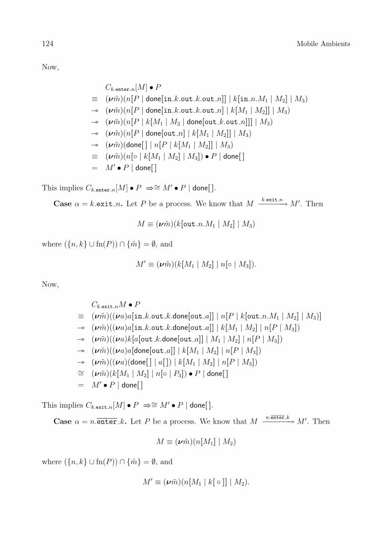
124 Mobile Ambients

Now,

Ck.enter n[M ] • P

≡ (νm)(n[P | done[in k.out k.out n]] | k[in n.M1 |M2] |M3)

_ (νm)(n[P | done[in k.out k.out n] | k[M1 |M2]] |M3)

_ (νm)(n[P | k[M1 |M2 | done[out k.out n]]] |M3)

_ (νm)(n[P | done[out n] | k[M1 |M2]] |M3)

_ (νm)(done[ ] | n[P | k[M1 |M2]] |M3)

≡ (νm)(n[◦ | k[M1 |M2] |M3]) • P | done[ ]

= M ′ • P | done[ ]

This implies Ck.enter n[M ] • P =⇒∼= M ′ • P | done[ ].

Case α = k.exit n. Let P be a process. We know that Mk.exit n−−−−−−→M ′. Then

M ≡ (νm)(k[out n.M1 |M2] |M3)

where ({n, k} ∪ fn(P )) ∩ {m} = ∅, and

M ′ ≡ (νm)(k[M1 |M2] | n[◦ |M3]).

Now,

Ck.exit nM • P

≡ (νm)((νa)a[in k.out k.done[out a]] | n[P | k[out n.M1 |M2] |M3)]

_ (νm)((νa)a[in k.out k.done[out a]] | k[M1 |M2] | n[P |M3])

_ (νm)((νa)k[a[out k.done[out a]] |M1 |M2] | n[P |M3])

_ (νm)((νa)a[done[out a]] | k[M1 |M2] | n[P |M3])

_ (νm)((νa)(done[ ] | a[ ]) | k[M1 |M2] | n[P |M3])∼= (νm)(k[M1 |M2] | n[◦ | P3]) • P | done[ ]

= M ′ • P | done[ ]

This implies Ck.exit n[M ] • P =⇒∼= M ′ • P | done[ ].

Case α = n.enter k. Let P be a process. We know that Mn.enter k−−−−−−−→M ′. Then

M ≡ (νm)(n[M1] |M2)

where ({n, k} ∪ fn(P )) ∩ {m} = ∅, and

M ′ ≡ (νm)(n[M1 | k[ ◦ ]] |M2).

4.3. Characterising reduction barbed congruence 125

−1 ⊕−2 = (νo)(o[ ] | open o.−1 | open o.−2)

SPYα〈i, j,−〉 = (i[out n] | −)⊕ (j[out n] | −)if α ∈ {k.enter n, k.exit n, k.open n, ∗.enter n, ∗.exit n}

SPYα〈i, j,−〉 = (i[out k.out n] | −)⊕ (j[out k.out n] | −) if α ∈ {n.enter k}

Table 4.8: Auxiliary contexts and processes

Now,

Cn.enter k[M ] • P

≡ (νm)((νa)a[in n.k[out a.(P | (νb)b[out k.out n.done[out b]])]] | n[M1] |M2)

_ (νm)(n[M1 | (νa)a[k[out a.(P | (νb)b[out k.out n.done[out b]])]]] |M2)

_ (νm)(n[M1 | (νa)a[] | k[P | (νb)b[out k.out n.done[out b]]]] |M2)

_ (νm)(n[M1 | (νa)a[] | k[P ] | (νb)b[out n.done[out b]]] |M2)

_ (νm)(n[M1 | (νa)a[] | k[P ]] | (νb)b[done[out b]] |M2)

_ (νm)(n[M1 | (νa)a[] | k[P ]] | (νb)b[] | done[] |M2)∼= (νm)(n[M1 | k[ ◦ ]] |M2) • P | done[ ]

= M ′ • P | done[ ]

This implies Cn.enter k[M ] • P =⇒∼= M ′ • P | done[ ].

Case α = k.open n. Let P be a process. We know that Mk.open n−−−−−−→ M ′. Then

M ≡ (νm)(n[M1] | M2), where n ∈ {m}, and M ′ ≡ k[◦ | (νm)(M1 | M2)]. Names a and bare fresh for M . Now,

Ck.open n[M ] • P

≡ k[P | (νa, b)(open b.open a.done[out k] |a[(νm)(n[M1] |M2) | open n.b[out a]])]

_ k[P | (νa, b)(open b.open a.done[out k] | a[(νm)(M1 |M2) | b[out a]])]

_ k[P | (νa, b)(open b.open a.done[out k] | a[(νm)(M1 |M2)] | b[])]_ k[P | (νa, b)(open a.done[out k] | a[(νm)(M1 |M2)])]

_ k[P | (νa, b)(done[out k] | (νm)(M1 |M2))]

_ k[P | (νm)(M1 |M2))]done[]

≡ k[◦ | (νm)(M1 |M2)] • P | done[ ]

= M ′ • P | done[ ]

This implies Ck.open n[M ] • P =⇒∼= M ′ • P | done[ ]. �

126 Mobile Ambients

To complete the correspondence proof between actions α and their contexts Cα[−], wehave to prove the converse of Lemma 4.3.8, formalised in Lemma 4.3.11. Such result requiresa few technical definitions given in Table 4.8.

The symbol ⊕ denotes a form of internal choice, whereas the context SPYα〈i, j,−〉 is atechnical tool to guarantee that the process P provided by the environment does not performany action. This is necessary when proving completeness to guarantee that the contributionof P is the same on both sides. The ability of SPYα〈i, j, P 〉 to ‘spy’ on P stems fromthe fact that one of the two fresh barbs i and j is lost when P performs any action. Theproperty of SPYα〈i, j,−〉 is captured in the following lemma. As a useful shorthand, wewrite M ⇓ i1, . . . , in for M ⇓ i1 and · · · and M ⇓ in.

Lemma 4.3.9 Let M be a system which possibly contains an occurrence of the special process

◦. If M • SPYα〈i, j, P 〉τ−−→ O and O ⇓ i, j, where i, j are fresh for P and M , then there

exists a system M ′ such that:

1. O = M ′ • SPYα〈i, j, P 〉;

2. Mτ−−→M ′.

Proof For 1), the definition of • assures that there exists an arbitrary context C[−] suchthat C[SPYα〈i, j, P 〉] = M • SPYα〈i, j, P 〉, and names in P are not bound in C[−]. The

construction of SPYα〈i, j, P 〉 assures that if C[SPYα〈i, j, P 〉]τ−−→ Q, then either there is an

arbitrary context C ′ such that Q = C ′[SPYα〈i, j, P 〉], or Q = C[P ′] where SPYα〈i, j, P 〉τ−−→

P ′. But if SPYα〈i, j, P 〉τ−−→ P ′, then P ′ ⇓ i 6⇓ j, or P ′ ⇓ j 6⇓ i. As O ⇓ i, j, O must be the

outcome of the first reduction, and as such there exists an arbitrary context C ′[−] such that

O = C ′[SPYα〈i, j, P 〉]. Let M ′ = C ′[◦]. As C[SPYα〈i, j, P 〉]τ−−→ C ′[SPYα〈i, j, P 〉], names

in P cannot be bound in C ′[−]. This implies O = C ′[SPYα〈i, j, P 〉] = M ′ • SPYα〈i, j, P 〉, asrequired for 1).

For 2), M • SPYα〈i, j, P 〉 = C[SPYα〈i, j, P 〉]τ−−→ C ′[SPYα〈i, j, P 〉] = M ′ • SPYα〈i, j, P 〉

implies M = C[◦] τ−−→ C ′[◦] = M ′, as required. �

We also need a simple result on arbitrary contexts.

Lemma 4.3.10 Let C[−] and C ′[−] be arbitrary contexts, P, P ′ processes, and r a fresh

name for C[−] and P , such that C[r[P ]]τ−−→ C ′[r[P ′]]. Then C[0]

τ−−→ C ′[0].

We can finally prove the correspondence between actions and contexts.

Lemma 4.3.11 Let M be a system, let α ∈ {k.enter n, k.exit n, n.enter k, k.open n},and let i, j be fresh names for M . For all processes P with {i, j} ∩ fn(P ) = ∅, if Cα[M ] •SPYα〈i, j, P 〉 =⇒∼= O | done[ ] and O ⇓ i, j, then there exists a system M ′ such that O ∼=M ′ • SPYα〈i, j, P 〉 and M

α==⇒M ′.

Proof The proof depends on the precise definition of the context. The main argument isthat in the reduction

Cα[M ] • SPYα〈i, j, P 〉 =⇒∼= O | done[ ]

the fresh ambient done[ ] can only be unleashed if M performs the action α, possibly precededor followed by some internal actions. The fresh barbs i, j assure that the process P does not

4.3. Characterising reduction barbed congruence 127

take part in the reduction, and that the component SPYα〈i, j, P 〉 is found intact after thereduction. The barbed congruence is used to garbage collect a possible (νa)a[ ] ambient. Weproceed by case analysis on α.

Case α = k.enter n. Observe that

Cα[M ] • SPYα〈i, j, P 〉 = n[SPYα〈i, j, P 〉 | done[in k.out k.out n]] |M .

As O ⇓ i, j and done is fresh, by several applications of Lemma 4.3.9, there must be a systemcontext D[−] such that O | done[ ] ≡ D[done[ ]] •SPYα〈i, j, P 〉 and Cα[M ] =⇒ D[done[ ]]. AsP cannot reduce and done is fresh, the ambient n does not migrate during the reduction.Moreover, as M is a system, the ambient n cannot be opened. Also observe that the ambientdone must consume the prefix in k, thus requiring the presence of an ambient k inside theambient n during the reduction. More precisely, there exist systems M1 and M2 and a staticcontext C[−] such that:

Cα[M ] • SPYα〈i, j, P 〉= n[SPYα〈i, j, P 〉 | done[in k.out k.out n]] |M

=⇒ τ−−→ (νm)(n[SPYα〈i, j, P 〉 | done[in k.out k.out n] |M1] |M2)τ−−→ (νm)(n[SPYα〈i, j, P 〉 | C[done[out k.out n]]] |M2)

=⇒ D[done[ ]] • SPYα〈i, j, P 〉≡ D[0] • SPYα〈i, j, P 〉 | done[ ]

≡ O | done[ ]

Examining the above reductions sequence from Cα[M ] • SPYα〈i, j, P 〉 we conclude that

M =⇒ k.enter n−−−−−−−→ (νm)(n[◦ |M1] |M2).

As the name done is fresh for M , by several applications of Lemma 4.3.10, we also have that

(νm)(n[◦ | 0 |M1] |M2) • SPYα〈i, j, P 〉 =⇒ D[0] • SPYα〈i, j, P 〉.

Repeated application of Lemma 4.3.9(2) gives (νm)(n[◦ | 0 | M1] | M2) =⇒ D[0], and

therefore, as ≡ is closed under reduction, there is a M ′, M ′ ≡ D[0], such that Mk.enter n

=======⇒M ′, as desired.

Case α = k.exit n. Observe that

Ck.exit n[M ] • SPYα〈i, j, P 〉 = (νa)a[in k.out k.done[out a]] | n[SPYα〈i, j, P 〉 |M ] .

To unleash the ambient done, the ambient a must perform both its capabilities, and as itsname is restricted the ambient a will be empty at the end of reduction. As P cannot reduce,and M is a system, the ambient n does not migrate during the reduction. Also observe thatthe ambient a must consume the prefix in k, thus requiring the presence of an ambient k at

128 Mobile Ambients

top-level. More precisely, there exist a system M1 and a static contexts D[−] and E[−] suchthat:

Ck.exit n[M ] • SPYα〈i, j, P 〉= (νa)a[in k.out k.done[out a]] | n[SPYα〈i, j, P 〉 |M ]

=⇒ (νa)a[in k.out k.done[out a]] |M1 • SPYα〈i, j, P 〉τ−−→ (νa)D[a[out k.done[out a]]] • SPYα〈i, j, P 〉=⇒ (νa)E[done[ ] | a[ ]] • SPYα〈i, j, P 〉 (?)∼= E[0] • SPYα〈i, j, P 〉 | done[ ]

≡ O | done[ ]

Examining the above reductions sequence from Ck.exit n[M ]•SPYα〈i, j, P 〉 we conclude that

M =⇒ k.exit n−−−−−−→M1.

As the name done is fresh for M , by several applications of Lemma 4.3.10 to the reductionmarked by (?) we have:

(νa)a[in k.out k.0] |M1 • SPYα〈i, j, P 〉 =⇒ (νa)E[0 | a[ ]] • SPYα〈i, j, P 〉 .

Again, as a is fresh, by several applications of Lemma 4.3.10, and reducing underneath (νa),we obtain:

(νa)(0 |M1) • SPYα〈i, j, P 〉 =⇒ (νa)E[0 | 0] • SPYα〈i, j, P 〉 .

Summarising,

M1 • SPYα〈i, j, P 〉 ≡ (νa)(0 |M1) • SPYα〈i, j, P 〉 =⇒ (νa)E[0 | 0] • SPYα〈i, j, P 〉

and, as ≡ is closed under reductions,

M1 =⇒≡ E[0] .

So, assuming M ′ = E[0], we can conclude.

Case α = n.enter k. Observe that

Cα[M ] • SPYα〈i, j, P 〉 =(νa)a[in n.k[out a.(SPYα〈i, j, P 〉 | (νb)b[out k.out n.done[out b]])]] |M

To unleash the ambient done, the ambient a must use its in n capability, and the ambient bmust exit from a. Moreover the ambient b must unleash all its capabilities. This implies thatat the end of the reduction both secret ambients a and b will be empty. Also observe thatthe prefix in n must be consumed, thus requiring the presence of an ambient n at top-level.

4.3. Characterising reduction barbed congruence 129

More precisely, there exist a system M1 and static contexts D[−] and E[−] such that

Cn.enter k[M ] • SPYα〈i, j, P 〉= (νa)a[in n.(k[out a.(SPYα〈i, j, P 〉 | (νb)b[out k.out n.done[out b]])])] |M=⇒ (νa)a[in n.(k[out a.(SPYα〈i, j, P 〉 | (νb)b[out k.out n.done[out b]])])] |M1τ−−→ D[(νa)a[k[out a.(SPYα〈i, j, P 〉 | (νb)b[out k.out n.done[out b]]])]]

=⇒ E[done[] | (νb)b[ ]] • SPYα〈i, j, P 〉 (?)∼= E[done[]] • SPYα〈i, j, P 〉∼= E[0] • SPYα〈i, j, P 〉 | done[]

= O | done[ ]

Observe that,

D[(νa)a[k[out a.(SPYα〈i, j, P 〉 | (νb)b[out k.out n.done[out b]]])]]∼= D[k[SPYα〈i, j, P 〉 | (νb)b[out k.out n.done[out b]]]]

Thus, by examining the above reductions sequence from Cn.enter k[M ] • SPYα〈i, j, P 〉 weconclude that

M =⇒ n.enter k−−−−−−−→∼= D[k[ ◦ ]].

As the name done is fresh, several applications of Lemma 4.3.10 to the above reductionmarked by (?) gives:

D[(νa)a[k[out a.(SPYα〈i, j, P 〉 | (νb)b[out k.out n.0])]]]

=⇒ E[0 | (νb)b[ ]] • SPYα〈i, j, P 〉 .

Again, as b is fresh, by several applications of Lemma 4.3.10 and reducing underneath (νb),we have:

D[(νa)a[k[out a.(SPYα〈i, j, P 〉 | 0)]]] =⇒ E[0 | 0] • SPYα〈i, j, P 〉 .

Summarising,

D[k[SPYα〈i, j, P 〉]] ∼= D[(νa)a[k[out a.(SPYα〈i, j, P 〉 | 0)]]] =⇒∼= E[0] • SPYα〈i, j, P 〉.

and, as ∼= is closed under reduction, this implies:

D[k[ ◦ ]] • SPYα〈i, j, P 〉 = D[k[SPYα〈i, j, P 〉]] =⇒≡ E[0] • SPYα〈i, j, P 〉.

Now, by applying Lemma 4.3.9 there must be a system M such that: D[k[ ◦ ]] =⇒ M andM • SPYα〈i, j, P 〉 ∼= E[0] • SPYα〈i, j, P 〉. Finally, as

M =⇒ n.enter k−−−−−−−→∼= D[k[ ◦ ]]

and ∼= is reduction closed, there must exist M ′ such that M =⇒M ′ and

M ′ • SPYα〈i, j, P 〉 ∼= E[0] • SPYα〈i, j, P 〉 ∼= O

130 Mobile Ambients

as required.

Case α = k.open n. Observe that

Ck.open n[M ] • SPYα〈i, j, P 〉 =k[SPYα〈i, j, P 〉 | (νa, b)(open b.open a.done[out k] | a[M | open n.b[out a]])]

where a and b are fresh. To unleash the ambient done, the ambient a must use its open ncapability, and the ambient b must exit from a. Moreover both the empty ambients a andb will be opened before done is activated. Also observe that the prefix open n must beconsumed, thus requiring the presence of an ambient n inside the ambient a. More precisely,there exist a system M1, processes Qi, and a static context D[−] such that:

Ck.open n[M ] • SPYα〈i, j, P 〉= k[SPYα〈i, j, P 〉 | (νa, b)(open b.open a.done[out k] | a[M | open n.b[out a]])]

=⇒ k[SPYα〈i, j, P 〉 | (νa, b)(open b.open a.done[out k] | a[M1 | open n.b[out a]])]τ−−→ k[SPYα〈i, j, P 〉 | (νa, b)(open b.open a.done[out k] | a[Q | b[out a]])]

=⇒ k[SPYα〈i, j, P 〉 | (νa, b)(open b.open a.done[out k] | a[Q1 | b[out a]])]τ−−→ k[SPYα〈i, j, P 〉 | (νa, b)(open b.open a.done[out k] | b[ ] | a[Q1])]

=⇒ k[SPYα〈i, j, P 〉 | (νa, b)(open b.open a.done[out k] | b[ ] | a[Q2])]τ−−→ k[SPYα〈i, j, P 〉 | (νa, b)(open a.done[out k] | 0 | a[Q2])]

=⇒ k[SPYα〈i, j, P 〉 | (νa, b)(open a.done[out k] | 0 | a[Q3])]

=⇒ k[SPYα〈i, j, P 〉 | (νa, b)(done[out k] | 0 | Q3)]

=⇒ D[done[ ]] • SPYα〈i, j, P 〉≡ D[0] • SPYα〈i, j, P 〉 | done[ ]

= O | done[ ]

Examining the above reductions sequence from Ck.open n[M ]•SPYα〈i, j, P 〉 we conclude that

M =⇒k.open n−−−−−−→ k[◦ | Q].

Ask[SPYα〈i, j, P 〉 | (νa, b)(open b.open a.done[out k] | a[Q | b[out a]])]=⇒ D[done[ ]] • SPYα〈i, j, P 〉

and the name done is fresh, by several applications of Lemma 4.3.10 we have

k[SPYα〈i, j, P 〉 | (νa, b)(open b.open a.0 | a[Q | b[out a]])]=⇒ D[0] • SPYα〈i, j, P 〉.

By Lemma 4.3.9, this implies

k[◦ | (νa, b)(open b.open a.0 | a[Q | b[out a]])] =⇒ D[0].

Applying our proof techniques we can easily prove that:

k[◦ | (νa, b)(open b.open a.0 | a[Q | b[out a]])] ∼= k[◦ | Q].

4.3. Characterising reduction barbed congruence 131

As ∼= is closed under reduction, it follows that there is M ′ such that

k[◦ | Q] =⇒M ′ ∼= D[0].

So, there is M ′ such that M =⇒M ′ and O ∼= M ′ • SPYα〈i, j, P 〉, as desired.�

Theorem 4.3.12 (Completeness) Reduction barbed congruence is contained in late bisim-ilarity.

Proof We prove that the relation R = {(M, N) | M ∼= N} is a late bisimulation. Theresult will then follow by co-induction.

• Suppose M R N . Suppose also that Mα−−→ M ′, with α ∈ {k.enter n, k.exit n,

n.enter k, k.open n}. We must find a system N ′ such that Nα

==⇒ N ′ and for all P ,M ′ • P ∼= N ′ • P .

The idea of the proof is to use a particular context which mimics the effect of theaction α, and also allows us to subsequently compare the residuals of the two systems.This context has the form

Dα〈P 〉[−] = (Cα[−] | Flip) • SPYα〈i, j, P 〉

where Cα[−] are the contexts in Table 4.7 and Flip is the system:

(νk)k[in done.out done.(succ[out k]⊕ fail[out k])]

with succ and fail are fresh names. Intuitively, the existence of the fresh barb failindicates that the action α has not yet happened, whereas the presence of succ togetherwith the absence of fail ensures that the action α has been performed, and has beenreported via done.

As ∼= is contextual, M ∼= N implies that, for all processes P , it holds

Dα〈P 〉[M ] ∼= Dα〈P 〉[N ] .

By Lemma 4.3.8, and by inspecting the reduction of the Flip process, we observe that:

Dα〈P 〉[M ] =⇒∼= M ′ • SPYα〈i, j, P 〉 | done[ ] | Flip=⇒∼= M ′ • SPYα〈i, j, P 〉 | done[ ] | succ[ ]

where M ′ • SPYα〈i, j, P 〉 | done[ ] | succ[ ] ⇓ i, j, succ 6⇓ fail. Call this outcome O1.

This reduction must be matched by a corresponding reduction

Dα〈P 〉[N ] =⇒ O2

where O1∼= O2. However, the possible matching reductions are constrained by the

barbs of O1, because it must hold O2 ⇓ i, j, succ 6⇓ fail.

As O2 ⇓ succ 6⇓ fail, it must be O2∼= N | done[ ] | succ[ ], for some systems N .

132 Mobile Ambients

As O2 ⇓ i, j, the previous observation can be combined with Lemma 4.3.11 to derivethe existence of a system (over the extended process syntax) N ′ such that N ∼= N ′ •SPYα〈i, j, P 〉 and a weak action

Nα

==⇒ N ′.

To conclude we must establish that for all P , it holds M ′ • P ∼= N ′ • P . As barbedcongruence is preserved by restriction, we have (νdone, succ)O1

∼= (νdone, succ)O2. As(νdone)done[ ] ∼= (νsucc)succ[ ] ∼= 0, it follows that

M ′ • SPYα〈i, j, P 〉 ∼= N ′ • SPYα〈i, j, P 〉.

Again, ∼= is preserved by restriction and (νi, j)SPYα〈i, j, P 〉 ∼= P . So, we can finallyderive M ′ • P R N ′ • P , for all processes P .

• Suppose now M R N and M∗.enter n−−−−−−−→ M ′, We must find a system N ′ such that

N | n[ ◦ ] =⇒ N ′ and for all P , M ′ • P ∼= N ′ • P .

We consider the context

C〈P 〉[−] = − | n[SPY∗.enter n〈i, j, P 〉] .

Because ∼= is contextual, for all processes P it holds

C〈P 〉[M ] ∼= C〈P 〉[N ] .

By inspecting the reduction rules of C〈P 〉[M ] we observe that,

C〈P 〉[M ] =⇒ M ′ • SPY∗.enter n〈i, j, P 〉

where M ′ • SPY∗.enter n〈i, j, P 〉 ⇓ i, j. Call this outcome O1.

This reduction must be matched by a corresponding reduction

C〈P 〉[N ] =⇒ O2

where O1∼= O2 and O2 ⇓ i, j. By several applications of Lemma 4.3.9 it follows that

there is a system N ′ such that O2 = N ′ • SPY∗.enter n〈i, j, P 〉 and N | n[ ◦ ] =⇒ N ′.Again, as ∼= is preserved by restriction and (νi, j)SPY∗.enter n〈i, j, P 〉 ∼= P , from O1

∼=O2 and the freshness of i and j we can derive M ′ • P ∼= N ′ • P , for all P , as required.

• Suppose at last MRN and M∗.exit n−−−−−−→ M ′. In this case we must find a system N ′

such that n[◦ | N ] =⇒ N ′ and for all P , M ′ • P ∼= N ′ • P .

We consider the context

C〈P 〉[−] = n[− | SPY∗.exit n〈i, j, P 〉] .

Because ∼= is contextual, for all processes P it holds

C〈P 〉[M ] ∼= C〈P 〉[N ] .

4.4. Up-to proof techniques 133

By inspecting the reduction rules of C〈P 〉[M ] we observe that,

C〈P 〉[M ] =⇒ M ′ • SPY∗.exit n〈i, j, P 〉

where M ′ • SPY∗.exit n〈i, j, P 〉 ⇓ i, J . Call this outcome O1.

This reduction must be matched by a corresponding reduction

C〈P 〉[N ] =⇒ O2

where O1∼= O2 and O2 ⇓ A, B. By several applications of Lemma 4.3.9 it follows that

there is a system N ′ such that O2 = N ′ • SPY∗.enter n〈i, j, P 〉 and n[◦ | N ] =⇒ N ′.Again, as ∼= is preserved by restriction and (νi, j)SPY∗.exit n〈i, j, P 〉 ∼= P , from O1

∼=O2 and the freshness of i and j we can derive M ′ • P ∼= N ′ • P , for all P , as required.

This concludes the analysis. �

As a consequence:

Theorem 4.3.13 Late bisimilarity, early bisimilarity, and reduction barbed congruence co-incide.

Proof Theorem 4.3.7 states that ≈⊆≈e and ≈e⊆∼=. Theorem 4.3.12 states the reductionbarbed congruence is contained in late bisimilarity, that is∼=⊆≈. We hence have the followingchain of inclusions ∼=⊆≈⊆≈e⊆∼=. �

A remark on transitivity of bisimilarity. Giving a direct proof that bisimilarity is atransitive relation seems to be awkward. At the same time, none of the Lemmas and The-orems used to prove that bisimilarity coincides with reduction barbed congruence requiresthe transitivity of the bisimilarity. This implies that late bisimilarity and early bisimilarityare equivalence relations.

The LTS can be presented in ‘very early’ style as done in [MH01]. See [ZN03]. With thisformulation, transitions report explicitly the process running inside the interacting ambient.The LTS in ‘very early’ style allows a straightforward proof of transitivity of bisimilarity.Again, the resulting labelled bisimilarity coincides with reduction barbed congruence, thusstrengthening the conjecture that in higher-order process calculi early and late bisimilaritycoincide.

4.4 Up-to proof techniques

In the previous section we gave a labelled characterisation of reduction barbed congruence toprove that two systems have the same behaviour. In this section we adapt some well-knownup-to proof techniques [MS92, San98] to our setting. These techniques allow us to reducethe size of the relation R to exhibit to prove that two processes are bisimilar. We focus onthe up-to expansion [SM92] and the up-to context techniques [San96b]. As in the π-calculus,these two techniques can also be merged.

The expansion [AKH92], written ., is an asymmetric variant of the bisimilarity thatallows us to count the number of silent moves performed by a process. More precisely,M . N holds if M and N are bisimilar and N has at least as many τ -moves as M . Formally,

134 Mobile Ambients

Definition 4.4.1 (Expansion) A relation R over systems is an expansion if M R Nimplies:

• if Mα−−→ M ′, α 6∈ {∗.enter n, ∗.exit n}, then there exists a system N ′ such that

Nα

==⇒ N ′ and for all processes P it holds M ′ • P R N ′ • P ;

• if M∗.enter n−−−−−−−→ M ′ then there exists a system N ′ such that N | n[ ◦ ] =⇒ N ′ and for

all processes P it holds M ′ • P R N ′ • P ;

• if M∗.exit n−−−−−−→ M ′ then there exists a system N ′ such that n[◦ | N ] =⇒ N ′ and for all

processes P it holds M ′ • P R N ′ • P ;

• if Nα−−→ N ′, α 6∈ {∗.enter n, ∗.exit n}, then there exists a system M ′ such that

Mα−−→M ′ and for all processes P it holds M ′ • P R N ′ • P ;

• if N∗.enter n−−−−−−−→ N ′ then (M | n[P ]) R N ′ • P , for all processes P ;

• if N∗.exit n−−−−−−→ N ′ then n[M | P ] R N ′ • P , for all processes P .

We write M . N , if M R N for some expansion R.

Definition 4.4.2 (Bisimulation up to &) A symmetric relation R is a bisimulation upto & if M R N implies:

• if Mα−−→ M ′, α 6∈ {∗.enter n, ∗.exit n}, then there exists a system N ′ such that

Nα

==⇒ N ′ and for all processes P it holds M ′ • P &R. N ′ • P ;

• if M∗.enter n−−−−−−−→ M ′ then there exists a system N ′ such that N | n[ ◦ ] =⇒ N ′ and for

all processes P it holds M ′ • P &R. N ′ • P ;

• if M∗.exit n−−−−−−→ M ′ then there exists a system N ′ such that n[◦ | N ] =⇒ N ′ and for all

processes P it holds M ′ • P &R. N ′ • P .

Theorem 4.4.3 If R is a bisimulation up to &, then R ⊆≈.

The proofs of Theorem 4.4.3 and of Theorem 4.4.5 below can be easily derived from theproof of Theorem 4.4.7.

Definition 4.4.4 (Bisimulation up to context) A symmetric relation R is a bisimula-tion up to context if M R N implies:

• if Mα−−→ M ′′, α 6∈ {∗.enter n, ∗.exit n}, then there exists a system N ′′ such that

Nα

==⇒ N ′′, and for all processes P there is a system context C[−] and systems M ′ andN ′ such that M ′′ • P = C[M ′], N ′′ • P = C[N ′], and M ′ R N ′;

• if M∗.enter n−−−−−−−→ M ′′ then there exists a system N ′′ such that N | n[ ◦ ] =⇒ N ′′, and

for all processes P there is a system context C[−] and systems M ′ and N ′ such thatM ′′ • P = C[M ′], N ′′ • P = C[N ′], and M ′ R N ′;

4.4. Up-to proof techniques 135

• if M∗.exit n−−−−−−→ M ′′ then there exists a system N ′′ such that n[◦ | N ] =⇒ N ′′, and

for all processes P there is a system context C[−] and systems M ′ and N ′ such thatM ′′ • P = C[M ′], N ′′ • P = C[N ′], and M ′ R N ′.

Theorem 4.4.5 If R is a bisimulation up to context, then R ⊆≈.

Definition 4.4.6 (Bisimulation up to context and up to &) A symmetric relation Ris a bisimulation up to context and up to & if M R N implies:

• if Mα−−→ M ′′, α 6∈ {∗.enter n, ∗.exit n}, then there exists a system N ′′ such that

Nα

==⇒ N ′′, and for all processes P there is a system context C[−] and systems M ′ andN ′ such that M ′′ • P & C[M ′], N ′′ • P & C[N ′], and M ′ R N ′;

• if M∗.enter n−−−−−−−→ M ′′ then there exists a system N ′′ such that N | n[ ◦ ] =⇒ N ′′, and

for all processes P there is a system context C[−] and systems M ′ and N ′ such thatM ′′ • P & C[M ′], N ′′ • P & C[N ′], and M ′ R N ′;

• if M∗.exit n−−−−−−→ M ′′ then there exist a system N ′′ such that n[◦ | N ] =⇒ N ′′, and

for all processes P there is a system context C[−] and systems M ′ and N ′ such thatM ′′ • P & C[M ′], N ′′ • P & C[N ′], and M ′ R N ′.

Theorem 4.4.7 If R is a bisimulation up to context and up to &, then R ⊆≈.

Proof We define the relation S as the smallest relation such that:

1. M R N implies M S N ;

2. M & A, A S B, B . N implies M S N ;

3. M S N implies C[M ] S C[N ], for all system contexts C[−].

We prove by induction on its definition, that S is a late bisimulation. This will assure thesoundness of the relationR, because M R N implies M S N which implies M ≈ N . Observethat S is symmetric because R is.

• M S N because M R N .

Suppose that Mα−−→M ′′, with α 6∈ {∗.enter n, ∗.exit n}. As R is a bisimulation up

to context and up-to &, we know that there exists a system N ′′ such that Nα

==⇒ N ′′.We also know that for all process P , there exist a system context C[−] and systemsM ′ and N ′ such that M ′′ • P & C[M ′], N ′′ • P & C[N ′], and M ′ R N ′. This impliesM ′ S N ′. By construction S is contextual and C[M ′] S C[N ′] holds. By constructionS is closed under expansion, and therefore M ′′ S N ′′, as required.

Suppose that M∗.enter n−−−−−−−→M ′′. As R is a bisimulation up to context and up to &, we

know that there exists a system N ′′ such that N | n[ ◦ ]∗.enter n

=======⇒ N ′′. We also knowthat for all process P , there exist a system context C[−] and systems M ′ and N ′ suchthat M ′′ • P & C[M ′], N ′′ • P & C[N ′], and M ′ R N ′. This implies M ′ S N ′. By

136 Mobile Ambients

construction, S is contextual, and C[M ′] S C[N ′] holds. By construction S is closedunder expansion, and therefore M ′′ S N ′′, as required.

Suppose that M∗.exit n−−−−−−→M ′′. As R is a bisimulation up to context and up to &, we

know that there exists a system N ′′ such that n[◦ | N ]∗.exit n

=======⇒ N ′′. We also knowthat for all process P , there exist a system context C[−] and systems M ′ and N ′ suchthat M ′′ • P & C[M ′], N ′′ • P & C[N ′], and M ′ R N ′. This implies M ′ S N ′. Byconstruction, S is contextual, and C[M ′] S C[N ′] holds. By construction S is closedunder expansion, and we conclude M ′′ S N ′′, as required.

• M S N because M & A, A S B, B . N .

The induction hypothesis tells us that A S B behaves like a late bisimulation.

Suppose Mα−−→M ′, with α 6∈ {∗.enter n, ∗.exit n}. A simple diagram chasing allows

us to conclude that there are systems A′, B′, N ′ such that for all process P it holdsM ′ •P & A′ •P S B′ •P . N ′ •P , and in turn, by construction of S, M ′ •P S N ′ •P .

Suppose M∗.enter n−−−−−−−→ M ′. As M & A, for all process P , it holds M ′ • P & A | n[P ].

As A S B, the closure properties of S assure that A | n[P ] S B | n[P ]. The expansionrelation is a congruence, and since B S N we conclude that B | n[P ] . N | n[P ]. ButN | n[P ] =⇒ N | n[P ], and M ′ • P &S. (N | n[ ◦ ]) • P . This, by construction of S,implies M ′ • P S (N | n[ ◦ ]) • P .

Suppose M∗.exit n−−−−−−→ M ′. As M & A, for all process P , it holds M ′ • P & n[P | A].

As A S B, the closure properties of S assure that n[P | A] S n[P | B]. The expansionrelation is a congruence, and since B S N we conclude that n[P | A] . n[P | N ]. Butn[P | B] =⇒ n[P | N ], and M ′ • P &S. n[◦ | N ] • P . This, by construction of S,implies M ′ • P S n[◦ | N ] • P .

• C[M ] S C[N ] because M S N and C[−] is a system context.

The induction hypothesis tells us that (M, N) ∈ S is a pair satisfying the bisimulationconditions in S. Lemma 4.3.3 assures that the pair (C[M ], C[N ]) ∈ S satisfies thebisimulation conditions in S.

This completes the induction. �

4.5 Adding communication

The basic idea is to have an output process such as 〈E〉.P , which outputs the message Eand then continues as P , and an input process (x)Q which on receiving a message binds itto x in Q which then executes; here occurrences of x in Q are bound. Notice that we havesynchronous output; as discussed in [VC99, San01, BCC01a] this is not unrealistic becausecommunication in MA is always local. The syntax of our extended language, together withthe reduction rule for communication, is given in Table 4.9.

The LTS is extended by the introduction of two new pre-actions (E) for input, 〈−〉 foroutput, and a new form of concretions (νm)〈E〉Q. In Table 4.11 we give all the defining rules

4.5. Adding communication 137

Names: a, b, . . . , k, l, m, n, . . . ∈ N

Capabilities:C ::= in n may enter into n∣∣ out n may exit out of n∣∣ open n may open n

Expressions:E, F ::= x variable∣∣ C capability∣∣ E.F path∣∣ ε empty path

Guards:G ::= E expression∣∣ (x) input∣∣ 〈E〉 output

Systems:M, N ::= 0 termination∣∣ M1 |M2 parallel composition∣∣ (νn)M restriction∣∣ n[P ] ambient

Processes:P, Q,R ::= 0 nil process∣∣ P1 | P2 parallel composition∣∣ (νn)P restriction∣∣ G.P prefixing∣∣ n[P ] ambient∣∣ !G.P replication

Structural and Reduction rules for Communication:E.(F.P ) ≡ (E.F ).P (Struct Path)ε.P _ P (Red Empty Path)(x).P | 〈M〉.Q _ P [M/x] | Q (Red Comm)

Table 4.9: Message-passing Mobile Ambients in two levels

138 Mobile Ambients

Pre-actions: π ::= . . . Concretions: K ::= (νm)〈P 〉Q∣∣ (E)∣∣ 〈−〉 ∣∣ (νm)〈E〉Q

Table 4.10: Pre-actions and concretions for communication

(π Output)〈E〉.P

〈−〉−−−→ 〈E〉P

(π Input)(x).P

(E)−−−→ P [E/x]

(π Path)E.(F.P )

π−−→ Q

(E.F ).Pπ−−→ Q

(τ Eps)ε.P

τ−−→ P

(τ Comm) P〈−〉−−−→ (νm)〈E〉P ′ Q

(E)−−−→ Q′ fn(Q′) ∩ {m} = ∅

P | Q τ−−→ (νm)(P ′ | Q′)

Table 4.11: Labelled transition system: communication

that should be added to those of Table 4.4 and Table 4.5 to obtain the LTS for the extendedcalculus. Note that in the structural rules of Table 4.4 we are now assuming that parallelcomposition and restriction distribute over the new form of concretions (νm)〈E〉Q in thesame manner as (νm)〈P 〉Q. The slightly unusual pre-action for output allows a uniformtreatment of extrusion of names.

The proof of Theorem 4.2.3 can be easily completed to take into account the extendedcalculus. A consequence of working with MA in two levels is that communication capabil-ities cannot be observed at top-level. Moreover, the free variables of a system cannot beinstantiated by a system context, because in a system context the hole cannot appear undera prefix. This in turn implies that our bisimulations can be applied to the extended calculus,and all the results of Section 4.3 and Section 4.4 hold without modifications.

Theorem 4.5.1 Late bisimilarity, early bisimilarity, and reduction barbed congruence coin-cide in the Message Passing Calculus.

Theorem 4.5.2 The up-to expansion, up-to context, and up-to context and expansion prooftechniques are sound proof techniques in the Message Passing Calculus.

4.6 Algebraic theory

In this section we prove a collection of algebraic properties using our bisimulation proofmethods. Then, we prove the correctness of a protocol for controlling access through afirewall, first proposed in [CG00b].

We briefly comment on the laws of Theorem 4.6.1. We recall that M, N range over sys-tems and P, Q,R over processes. The first two laws are two examples of local communication

4.6. Algebraic theory 139

within private ambients without interference. The third law is the well-known perfect fire-wall law. The following four laws represent non-interference properties about movements ofprivate ambients. Finally, the last two laws describe when opening cannot be interfered.

As a convenient notation, we write∏

j∈J Pj for P1 | . . . | Pj. We also write R= for thesymmetric closure of R.

Theorem 4.6.1

1. (νn)n[〈W 〉.P | (x).Q |M ] ∼= (νn)n[P | Q[W/x] |M ] if n 6∈ fn(M)

2. (νn)n[〈W 〉.P | (x).Q |∏

j∈J open kj.Rj] ∼= (νn)n[P | Q[W/x] |∏

j∈J open kj.Rj]

3. (νn)n[P ] ∼= 0 if n 6∈ fn(P )

4. (νn)((νm)m[in n.P ] | n[M ]) ∼= (νn)n[(νm)m[P ] |M ] if n 6∈ fn(M)

5. (νm,n)(m[in n.P ] | n[∏

j∈J open kj.Rj]) ∼= (νm, n)n[m[P ] |∏

j∈J open kj.Rj]

6. (νn)n[(νm)m[out n.P ] |M ] ∼= (νn)((νm)m[P ] | n[M ]) if n 6∈ fn(M)

7. (νn)n[m[out n.P ] |∏

j∈J open kj.Rj] ∼= (νn)(m[P ] | n[∏

j∈J open kj.Rj]) if m 6=kj, for j ∈ J

8. n[(νm)(open m.P | m[N ]) | Q] ∼= n[(νm)(P | N) | Q] if Q ≡ M |∏

j∈J〈Wj〉.Rj

and m 6∈ fn(N)

9. (νn)n[(νm)(open m.P | m[Q]) | R] ∼= (νn)n[(νm)(P | Q) | R] if R ≡∏

i∈I〈Wi〉.Si |∏j∈J open kj.Rj and m, n 6∈ fn(Q).

Proof To prove the above laws, except (3) and (9), we exhibit the appropriate bisimula-tion. In all cases the bisimulation has a similar form:

S = {(lhs, rhs)}= ∪ ≈

where lhs and rhs denote respectively the left hand side and the right hand side of theequation, parameterised over names, processes and systems. For proving the laws (3) and(9) we show that the above S is a bisimulation up to context and up to structural congruence.We illustrate the proof of the law (3). Let S = {((νn)n[Q],0) | ∀Q s.t. n 6∈ fn(Q)}=. Weshow that S is a bisimulation up to context and up to structural congruence. The mostdelicate cases are those regarding the silent moves ∗.enter k and ∗.exit k. For instance, if

(νn)n[P ]∗.enter k−−−−−−−→ (νn)k[◦ | n[P ′]] ≡ k[◦ | (νn)n[P ′]]

then

0 | k[ ◦ ] =⇒≡ k[◦ | 0]

and up to context and structural congruence we are still in S. �

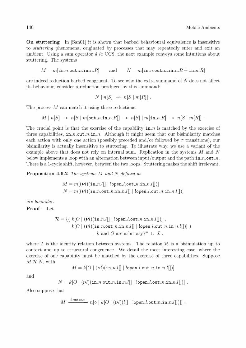
140 Mobile Ambients

On stuttering In [San01] it is shown that barbed behavioural equivalence is insensitiveto stuttering phenomena, originated by processes that may repeatedly enter and exit anambient. Using a sum operator a la CCS, the next example conveys some intuitions aboutstuttering. The systems

M = m[in n.out n.in n.R] and N = m[in n.out n.in n.R + in n.R]

are indeed reduction barbed congruent. To see why the extra summand of N does not affectits behaviour, consider a reduction produced by this summand:

N | n[S] _ n[S | m[R]] .

The process M can match it using three reductions:

M | n[S] _ n[S | m[out n.in n.R]] _ n[S] | m[in n.R] _ n[S | m[R]] .

The crucial point is that the exercise of the capability in n is matched by the exercise ofthree capabilities, in n.out n.in n. Although it might seem that our bisimilarity matcheseach action with only one action (possibly preceded and/or followed by τ transitions), ourbisimilarity is actually insensitive to stuttering. To illustrate why, we use a variant of theexample above that does not rely on internal sum. Replication in the systems M and Nbelow implements a loop with an alternation between input/output and the path in n.out n.There is a 1-cycle shift, however, between the two loops. Stuttering makes the shift irrelevant.

Proposition 4.6.2 The systems M and N defined as

M = m[(νl)(in n.l[] | !open l.out n.in n.l[])]

N = m[(νl)(in n.out n.in n.l[] | !open l.out n.in n.l[])]

are bisimilar.

Proof Let

R = {( k[O | (νl)(in n.l[] | !open l.out n.in n.l[])] ,

k[O | (νl)(in n.out n.in n.l[] | !open l.out n.in n.l[])] )

| k and O are arbitrary}= ∪ I .

where I is the identity relation between systems. The relation R is a bisimulation up tocontext and up to structural congruence. We detail the most interesting case, where theexercise of one capability must be matched by the exercise of three capabilities. SupposeM R N , with

M = k[O | (νl)(in n.l[] | !open l.out n.in n.l[])]

andN = k[O | (νl)(in n.out n.in n.l[] | !open l.out n.in n.l[])] .

Also suppose that

Mk.enter n−−−−−−−→ n[◦ | k[O | (νl)(l[] | !open l.out n.in n.l[])]] .

4.6. Algebraic theory 141

Then N can perform the following sequence of transitions:

Nk.enter n−−−−−−−→ n[◦ | k[O | (νl)(out n.in n.l[] | !open l.out n.in n.l[])]]τ−−→ n[ ◦ ] | k[O | (νl)(in n.l[] | !open l.out n.in n.l[])]τ−−→ n[◦ | k[O | (νl)(l[] | !open l.out n.in n.l[])]] .

For all instantiations of ◦ we can factor out the context n[◦ | −] and up to context we arestill in R. �

The proof above clearly shows how the exercise of the three capabilities in n.out n.in nneeded to match the capability in n give rise to a k.enter n action followed by two internaltransitions. The internal actions are subsequently absorbed by the weak formulation of theequivalence.

Crossing a firewall A protocol is discussed in [CG00b] for controlling access through afirewall. The ambient w represents the firewall; the ambient m, a trusted agent containinga process Q that is supposed to cross the firewall. The firewall ambient sends into the agenta pilot ambient k with the capability in w for entering the firewall. The agent acquires thecapability by opening k. The process Q carried by the agent is finally liberated inside thefirewall by the opening of ambient m. Names m and k act like passwords which guaranteethe access only to authorised agents. Here is the protocol in MA:

AGdef= m[open k.(x).x.Q]

FWdef= (νw)w[open m.P | k[out w.in m.〈in w〉]]

The correctness (of a mild variant) of the protocol above is shown in [CG00b] for may-testing [DH84] proving that

(νm, k)(AG | FG) ∼= (νw)w[Q | P ]

under the conditions that w 6∈ fn(Q), x 6∈ fv(Q), {m, k} ∩ (fn(P ) ∪ fn(Q)) = ∅. The proofrelies on non-trivial contextual reasonings. In what follows, we show how it can be establishedusing our bisimulation proof methods.

The system on the right can be obtained from that one on the left by executing six τ -actions. So, it suffices to prove that ∼= is insensitive to all these τ -actions. The result followsfrom the algebraic laws of Theorem 4.6.1 and the following two laws:

Lemma 4.6.3 Let P , Q, and R be processes. Then

1. (νk, m, w)(k[in m.P ] | m[open k.Q] | w[open m.R])∼= (νk, m, w)(m[k[P ] | open k.Q] | w[open m.R])

2. (νm,w)(m[〈in w〉 | (x).P ] | w[open m.Q])∼= (νm,w)(m[P [in w/x]] | w[open m.Q])

142 Mobile Ambients

Proof By exhibiting the appropriate bisimulation. Again, in all cases the bisimulationhas a similar form:

S = {(lhs, rhs)}= ∪ ≈

where lhs and rhs denote respectively the left hand side and the right hand side of theequation. �

Theorem 4.6.4 If w 6∈ fn(Q), x 6∈ fv(Q), and {m, k} ∩ (fn(P ) ∪ fn(Q)) = ∅, then

(νm, k)(AG | FG) ∼= (νw)w[Q | P ].

Proof It suffices to apply the algebraic laws of Theorem 4.6.1 and Lemma 4.6.3. Moreprecisely, we apply, in sequence, Law (7) of Theorem 4.6.1, Law (1) of Lemma 4.6.3, Law(9) of Theorem 4.6.1, Law (2) of Lemma 4.6.3, and Laws (5) and (9) of Theorem 4.6.1. �

Notes and References

The Seal Calculus and Mobile Ambients are built on the idea that some ‘network aware-ness’ is required to model wide-area distributed mobile computation. An excellent surveyof process algebras with localities is offered by Section 4 of Castellani’s ‘Process Algebraswith Localities’ [Cas01]. We limit ourselves to a panoramic view of the state of the art inbisimulation proof techniques for languages involving mobility of code.

HOπ Work towards developing a clear understanding of the use of higher-order features inprocess languages began several years ago with various proposals for higher-order versions ofknown calculi. In the introduction we have discussed at length the difficulties encounteredby these ‘early approaches’. The difficulty arises in establishing the soundness of the prooftechnique, which is tantamount to establishing some sort of contextuality property.

Sangiorgi studied intensively HOπ and introduced context bisimulation. Context bisim-ulation involves quantifications over all contexts a process can interact with, and by doingso it ‘circumvents’ the difficulties to establish the contextuality of the bisimulation. Allthe first part of this thesis relies on the ideas behind context bisimulation. Furthermore,one of Sangiorgi’s achievements was to provide a translation of the higher-order language,which supports code mobility, to a first-order π-calculus which supports only name mobility.1

With the restriction to a language of finite types, the translation led to normal bisimulation,a bisimulation that coincides with context bisimulation but does not involve the universalquantification over the interacting contexts.

Recently, Jeffrey and Rathke [JR03] developed an alternative presentation of the labelledtransition system and a novel proof technique which allows them to remove the limitationon recursive types. The basic idea behind their work is to mimic the contribution of theinteracting context directly in the LTS. In this way, they can rely on a standard, well-understood, CCS-like bisimulation. To give an account of their technique, consider againthe LTS for MA we proposed in Section 4.2. Transitions introduce a placeholder which isinstantiated by an arbitrary process in the bisimulation game. Jeffrey and Rathke’s approachis to add rules to the LTS so that the placeholder behaves as an arbitrary process. As for now,Jeffrey and Rathke’s novel labelled transition system is deeply inspired by the translationof HOπ into π-calculus, and this makes it difficult to export their ideas to different processcalculi.

Mobile Ambients Higher-order LTSs for Mobile Ambients can be found in [CG96, GC02,Vig99, FMT01], but we are not aware of any form of bisimilarity defined using these LTSs.In [Sew03], Sewell addresses the problem of uniformly deriving LTSs and bisimulation con-gruences from the reduction rules of a calculus. The transitions generated for a fragment

1The existence of the translation indirectly implies that up-to proof techniques can be applied to HOπ,even if their correctness has not been proved in a direct way. (Sangiorgi, personal communication).

144 Notes and References

of Mobile Ambients require the same universal quantifications on the content of the inter-acting ambient as ours. Sewell’s techniques only apply to strong equivalences. A simplefirst-order labelled transition system for Mobile Ambients without restriction is proposed bySangiorgi in [San01]. Using this LTS the author defines an intensional bisimilarity for MAthat separates terms on the basis of their internal structure.

A new impetus to research on labelled bisimilarities for Ambient-like languages, hasbeen given by Merro and Hennessy in [MH02]. They give an LTS and a characterisationof reduction barbed congruence for a variant of Levi and Sangiorgi’s Safe Ambients, calledSAP.

Our work on Mobile Ambients is the natural prosecution of [MH02], where we tackle theoriginal problem: to provide bisimulation proof methods for Mobile Ambients. The maindifferences with respect to [MH02] are the following:

• SAP differs from MA for having co-capabilities and passwords, both features are es-sential to prove the characterisation result in SAP.• Our env-actions, unlike those in [MH02], are truly late, as they do not mention the

process provided by the environment. This process can be added later, when playingthe bisimulation game.• Our actions for ambient’s movement, unlike those in SAP, report the name of the

migrating ambient. For instance, in k.enter n we say that ambient k enters n. Theknowledge of k is necessary to make the action observable by the environment. This isnot needed in SAP, because movements can be observed by means of co-capabilities.• Co-capabilities also allow the observation of the movement of an ambient whose name

is private. As a consequence, the perfect firewall equation does not hold in SAP or inSafe Ambients. In MA, the movements of an ambient whose name is private cannotbe observed. This is why the perfect firewall equation holds.

It is interesting to notice that dialects of Mobile Ambients evolved closer to the Sealcalculus. SafeAmbients [LS00a] requires mobility to be the consequence of a process syn-chronisation. SafeAmbients with Passwords [MH02] requires that the mobility takes place on(what we can assimilate to) channels2. The very last step that distinguishes these Ambientvariations from Seal is that Seal uses objective mobility — the agent is sent by the sur-rounding environment — while in Ambient-based calculi mobility is subjective — the agentsends itself —. It seemed quite natural that results similar to those of Merro and Hennessycan be stated easily for Seals. This turned out to be ‘wishful thinking’, as we have seen inSections 3.3 and 3.4.

Locations and failures Locations are the basic observable entities in both Mobile Am-bients and the Seal Calculus and they play a fundamental role in interaction. A differentrole is played by locations in the Distributed Join Calculus [FGL+96] and in the simplestform of Dπ [RH97]. In these calculi locations provide an explicit support for specifyingthe distribution of resources. The locality structure is mostly descriptive: the routing ofmessages across remote locations is transparent, and locations cannot be directly observed.

2Merro and Hennessy also modify Levi and Sangiorgi’s calculus so that the coaction of an out n mustbe placed exactly as a receive action in Seal.

Notes and References 145

In other words, it is equivalent to run processes P and Q at two different machines, or torun the compound process P | Q at a single machine. As a consequence, to reason aboutprocesses it is possible to erase all the locality informations3 and relate the simple semantics(respectively the Join Calculus semantics or CCS semantics) to the distributed semantics.This is not longer true if these models are refined so that locations can fail. The crash ofa physical site causes the permanent failure of its processes. As a consequence, locationsbecome (partially) observable.

New calculi and labelled bisimilarities In Chapter 3, an investigation of the expectedbehavioural theories of the Seal’s dialects suggested us to focus on a particular dialect.In general, the definition of a new process calculus can only benefit from a study of itsbehavioural theory, and a tractable and/or rich behavioural theory can be used as a strongargument to advertise a new process calculus.

This is the case for the Calculus of Mobile Resources [GHS02] and for New Boxed Ambi-ents [BCMS]. In fact, together with its syntax and operational semantics, a characterisationof barbed congruence in terms of a labelled bisimilarity (in both cases a contextual bisimu-lation), is given. More than that, when research on the Calculus of Mobile Resources was ina preliminary stage, difficulties encountered in the definition of the labelled bisimilarity putforward alternative directions.

Typed equivalences Programming practise usually imposes a discipline on how variablesor names are used. When this discipline is not explicit in the language, ‘expected’ propertiesmay not hold, or the theory of the language may reveal not strong enough to prove them.Types can be used to make such disciplines explicit.

The use of types affects contextually-defined behavioural equivalences such as reductionbarbed congruence, because in a typed calculus the processes being compared must obey tothe same typing, and the contexts in which they are tested must be compatible with thistyping. Typically, in a typed calculus the class of legal contexts in which two processes maybe tested is smaller than in the untyped calculus.

The literature of types for mobile systems is huge, but most of the works define typesystems to ensure behavioural properties of terms, like security properties. We limit ourreview to ‘types to ensure behavioural equalities ’. Among the works that deserve to be men-tioned figure the already cited [LS00b], where a type system is used to assure that processesinside ambients are single threaded. This rule out some interferences, and allow the proof ofsome simple behavioural equalities between terms of Safe Ambients. The characterisation oftyped barbed congruence with a labelled bisimilarity presents new difficulties. Seminal workin this area has been carried over by Boreale and Sangiorgi for IO types [BS98], and to alesser extent by Pierce and Sangiorgi for polymorphic types [PS00]. In presence of higher-order computation, characterisations of typed barbed congruence have been developed byHennessy, Merro, and Rathke [HMR03] and by Hennessy, Rathke, and Yoshida [HRY03]. Inthese works, types implement dynamic policies of resource access control.

3In the Distributed Join Calculus a little care is required to rule out migration attempts towards one’sown sublocations, which may delay or block some processes.

146 Notes and References

The Heritage of the Seal Calculus

As one of the contributions of this thesis has been the development of the Seal Calculus, wewill review the influence that Seal had on other works in the field.

Location mobility as a result of process synchronisation was first introduced in Seal asa natural extension of π-calculus communication primitives. It was later introduced forambients by Levi and Sangiorgi in [LS00a], and then in several other Ambient variants. TheSeal calculus also had a direct influence on the design of Boxed Ambients [BCC01a, BCC01b],a variant of the Ambient calculus obtained by suppressing the open capability and where nonlocal communication are made possible by enriching the calculus with the communicationprimitives of the located Seal calculus. The communication primitives of the shared Sealcalculus, first defined in [CGZN01], were adapted to Boxed Ambients in [CBC02] in orderto ease static detection of insecure information flows. The difference in expressiveness of thecommunication primitives of the located and shared variant of the primitives is at the originof the NBA (New Boxed Ambients) calculus defined in [BCMS], which enriches the sharedchannel communication of Seal they borrow from [CGZN01] with name capturing receivingactions (however these are useful only because they conform to the ambient calculus modelwhere names are tightly bound to agents and are not modified by mobility: since in Seal thereceiving agents decide the name of incoming seals this feature is useless). The interactionpattern introduced in Seal for mobility of exiting agents is first used for ambients in [MH02].Seal has inspired the calculus of mobile resources of [GHS02] which inherits the interactionpattern for exiting agents and the fact that mobility takes place on the anonymous contentof locations. Finally Seal primitives are also at the basis of the definition of Boxed-π,an extension of the π-calculus for securely integrating trusted and untrusted off-the-shelfsoftware components [SV99, PJ03].

A process languageout of a semantic model:

towards a domain theory forconcurrency

5 new-HOPLA

The language new-HOPLA is a compact but expressive language for higher-order nonde-terministic processes. It extends the language HOPLA of Nygaard and Winskel ([NW02,NW03, NW, Nyg03]) with operators to handle dynamically generated names. Its definitionhas been guided by the development of a domain theory for concurrency: while in the previ-ous chapters we started from pre-existent process languages with the goal of equipping themwith a reasonable semantics, our aim here is to build a language on top of (what appear tobe) solid basis. This fits within a broader project of research, towards a fully fledged domaintheory for concurrency based on presheaf categories [NW, CW03].

The language new-HOPLA has an operational interpretation, and it is on its operationalaccount that we concentrate: behaviour of terms is again our main concern.

The language new-HOPLA can be roughly described as an extension of the simply typedλ-calculus with prefixing, sums, and constructs to manipulate dynamically generated names.The type of a process describes the possible (shapes of) computation paths that the processcan perform. More in detail, let s be the set of names currently known by both the processand the environment. Then a typing judgement

α1:N, . . . , αn:N; x1:P1, . . . , xn:Pn ` t : Q

means that the process t yields computation paths in Q once name variables α1, . . . , αn

are instantiated with names in s, and processes with computation paths in P1, . . . , Pn areassigned to the process variables x1, . . . , xn. The types P are built using function spaces,sum, an anonymous action prefix type, (a limited form of) product, and recursive definition.A special function space accounts for name-generation.

It is notable that although we can express many kinds of concurrent processes in thelanguage, the language itself does not have many features typical of process calculi built-in,beyond nondeterministic sum and prefix operations. In particular, parallel composition ofprocesses, a la CCS, and restriction, a la π-calculus, can be defined in new-HOPLA, butare not primitive constructs.

Overview The reader may like to look ahead to the operational presentation in Section 5.2and to the study of its behavioural theory in Section 5.3. In addition, Section 5.4 reportsencodings of π-calculus, polyadic π-calculus, and Mobile Ambients into new-HOPLA. Butwe start in Section 5.1 with an account of a domain theory for concurrency built on pathsets, mostly taken from [NW]. Indexing the denotational model allows us to take intoaccount name generation, and this lead us to an overview of the denotational semantics ofnew-HOPLA, fundamental to understand its design choices.

150 new-HOPLA

5.1 Domain theory for path sets

In the path semantics, processes are intuitively represented as collections of their compu-tation paths. Paths are elements of preorders (P,≤P), (Q,≤Q), . . . (also denoted P, Q, . . .)called path orders. Path orders function as process types, each describing the set of possiblepaths for processes of that type together with their sub-path ordering. A process of type P isthen represented as a downwards-closed subset X ⊆ P, called a path set. Path sets orderedby inclusion form the elements of the poset P which we will think of as a domain of meaningsof processes of type P.

The poset P has many interesting properties. First of all, it is a complete lattice withjoins given by union. In the sense of Hennessy and Plotkin [HP79], P is a nondeterministicdomain, with joins used to interpret nondeterministic sums of processes. Accordingly, givena family (Xi)i∈I of elements of P, we will often write Σi∈IXi for their join. A typical finitejoin is written X1 + · · · + Xn while the empty join is the empty set, the inactive process,written ∅.

A second important property of P is that any X ∈ P is the join of certain prime elementsbelow it; P is a prime algebraic complete lattice [NPW81]. Primes are down-closures yPp =

{p′ | p′ ≤P p} of individual elements of P, representing a process that may perform thecomputation path p. The map yP reflects as well as preserves order, so that p ≤P q if andonly if yPp ⊆ yPq, and thus yP embeds P in P. We clearly have yPp ⊆ X if and only if p ∈ X,and prime algebraicity of P amounts to saying that any X ∈ P is the union of its elements:

X =⋃p∈X

yPp . (5.1)

Finally, P is characterised abstractly as the free join-completion of P, meaning it is join-complete, and given any join complete poset C and a monotone map f : P → C, there is aunique join-preserving map f † : P→ C such that the diagram on the left below commutes.

P

f ##HHHHHHHH

yP // Pf†��

C

f †X =⋃

p∈X fp .(5.2)

We call f † the extension of f along yP. Uniqueness of f † follows from equation (5.1). Notice

that we may instantiate C to any poset of the form Q, drawing our attention to join-preserving maps P→ Q. We will now investigate what additional type structure is at hand.

Linear category Write Lin for the category with path orders P, Q, . . . as objects, andjoin-preserving maps P → Q as arrows. Lin can be understood as a categorical model ofclassical linear logic, and accordingly we call arrows of Lin linear maps. The involution oflinear logic, P⊥, is given by Pop. The tensor product of P and Q, denoted P⊗Q is given bythe product of preorders, P×Q. The function space from P to Q, denoted P( Q, is givenby Pop×Q. To justify this, observe that by the freeness property (5.2), join preserving maps

P→ Q are in bijective correspondence with monotone maps P→ Q. Also, each element Y of

5.1. Domain theory for path sets 151

Q can be represented using its characteristic function, a monotone map fY : Qop → 2 fromthe opposite order to the simple poset 0 < 1 such that Y = {q | fY q = 1} and Q ∼= [Qop,2].We then obtain the following chain by uncurrying:

[P, Q] ∼= [P, [Qop,2]] ∼= [P×Qop,2] = [(Pop ×Q)op,2] ∼= Pop ×Q . (5.3)

So the preorder Pop × Q provides a type for a function space from P to Q. On objectsP and Q, products (written P&Q) and coproducts are both given by P + Q, the disjoint

juxtaposition of preorders. An element of P + Q can be identified with a pair (X, Y ), with

X ∈ P and Y ∈ Q, which provides the projections π1 : P + Q → P and π2 : P + Q → Q.Injection maps in Lin derive from the obvious injections into the disjoint sum of preordersP+Q. The empty order O plays the roles of empty product and empty coproduct. Actually,arbitrary products and coproducts are obtained by the construction above. This collapse ofproducts and coproducts highlights that Lin has arbitrary biproducts.

While rich in structure, Lin does not support all operations associated with processlanguages. In fact, all maps are join preserving, and, unlike e.g. prefixing, always send theempty sum (the inactive process) to itself.

Continuous maps As a solution, following the discipline of linear logic, nonlinear mapscan be obtained as linear maps whose domain is under an exponential. One choice of asuitable exponential for Lin is got by taking (!P,�P) to be the set of finite path sets of Pwith order

P �P P ′ ⇔ ∀p ∈ P.∃p′ ∈ P ′.p ≤P p′

(e.g., the finite join-completion of P)—so !P can be thought of as consisting of compund

paths associated with several runs. There is an obvious map iP : !P→ P sending a finite set{p1, . . . , pn} to the join yPp1 + · · ·+ yPpn. Such finite sums of primes are the finite (compact,

isolated) elements of P. The map iP assumes the role of yP above. For any X ∈ P andP ∈ !P, we have iPP ⊆ X if and only if P �P X, and X is the directed join of the finiteelements below it:

X =⋃

P�PX

iPP . (5.4)

Further, P is the free directed join completion of !P (also called ideal completion). Thismeans that given any monotone map f : !P → C for some directed-join complete poset C,there is a unique directed-join preserving (i.e. Scott continuous) map f ‡ : P → C such thatthe diagram below commutes.

!P

f $$IIIIIIII

iP // Pf‡��

C

f ‡X =⋃

P�X fP .(5.5)

We call f ‡ the extension of f along iP. Uniqueness of f ‡ follows from 5.4. As before we canreplace C by a nondeterministic domain Q and by the freeness properties (5.1) and (5.4) we

obtain a bijective correspondence between linear maps !P→ Q and continuous maps P→ Q.

152 new-HOPLA

Continuous maps allow more process operations, including prefixing, to be expressed.An element of P ∈ !P consists of several, possibly no, computation paths of P. Therefore itcan intuitively be understood as describing a compound computation path associated withrunning several copies of a process of type P.

Our choice of exponentials defines a functor ! : Lin → Lin, that sends an object P into!P, and sends a linear arrow f : P→ Q into !f : !P→ !Q, the linear map sending a finite pathset X to the set of finite paths sets y such that y ⊆ f(X). Via (5.5) the map y!P : !P → !Pextends to a map ηP = y‡!P : P→ !P:

ηPX =⋃

P�X

y!PP

that is, ηP : P → !P is a continuous map that sends a path set X to the set of the finitepaths sets contained in X. This map provides a denotational counterpart of prefixing, seefor instance [NW].

Indexing Lin Continuous maps can be used to define a category1 that gives a fully abstractmodel for HOPLA [NW03]. Yet, one more step must be taken to take into account name-generation.

Following the ideas of [Sta96], there are two important observations which underlie thenature of the sought model.

1. The behaviour of a process depends only on a finite set of names which it contains,i.e. its support. So, for each set of names s we will have a model P(s) to interpret thebehaviour of processes of type P which only use the names in s.

2. The behaviour of a process is preserved by injective renaming of its (free) names. Thisimplies the existence, for each type P and for each injection i : s→inj s′, of a translationP(i) : P(s)→ P(s′) that relates the space of meanings P(s′) to that of P(s).

A convenient framework in which to formalise this uniform family of interpretations is interms of functor categories.

Definition 5.1.1 Define I to be the category of finite sets and injective functions. DefineLinI to be the category of functors from I to Lin and natural transformations.

To see why LinI is a good candidate for a domain theory of concurrency able to expressalso dynamically generated names, recall that to give a functor P : I → Lin is to give anindexed family (P(s))s∈obj(I) of path orders, together with families of linear maps (P(i) :P(s) → P(s′))i:s→s′ such that the naturality conditions hold. Functoriality and naturalitygive uniformity over varying name sets.

We will now investigate the type structure of the category LinI . Overloading the nota-tion, we will denote objects of LinI with P, Q, ....

1The category Cts has path orders P, Q, . . . as objects, and continuous maps P→ Q as arrows.

5.2. The language 153

As usual with functor categories, much (but not all) of the structure of Lin extends toLinI . In particular, tensor ⊗, product &, sum +, and exponential ! extend pointwise.2

Some constructions are instead proper to LinI . A basic one is the object of namesconstruction, that allows to see a set of names as an object of Lin. For that, define N :I → Lin to be the functor whose action at s returns s itself, seen as a flat order, and whose

action on arrows is N(i)X = {i(n) | n ∈ X} for i : s → s′ (remember that X ∈ N(s)). Inother words, N is given by the chain of inclusions I ↪→ Set ↪→ Lin.

The disjoint union of sets in I lifts to a symmetric monoidal closed structure on LinI ,following a Day-like construction [Day70]. The associated tensor is denoted � (pronouncefunny tensor). The intuition behind this construction is that in an object P � Q the twocomponents P and Q must have disjoint supports. A good illustration of this is provided bythe comparison of the objects N⊗ N and N� N:

N⊗ N(s) = {(n1, n2) | n1, n2 ∈ s} N� N(s) = {(n1, n2) | n1, n2 ∈ s and n1 6= n2} .

It is possible to construct several function spaces in LinI . Our attention is directed toN( P, and !P( Q, where( is the function space associated to ⊗.3

The function space associated to �, when its domain its restricted to the object of names,gives rise to the functor δ : LinI → LinI , called the shift functor. If s is a finite set, we writes + 1 for the ‘generic’ set obtained by adding a new element, denoted ∗s, to the set s. Forf : s→ s′, we write f + 1 : s + 1→ s′ + 1 for the function that acts like f on the elementsof s, and sends ∗s onto ∗s′ . The shift functor is then defined on objects as δP(s) = P(s + 1),and as δP(i) = P(i + 1) on arrows. Intuitively, it extends the set of the public names s witha new, fresh, name: regarded in this way, δ represents functions that will only accept a newname as input.

The constructions we have highlighted in LinI provide an interpretation for the types ofnew-HOPLA: we move further to examine their operational interpretation.

5.2 The language

The language new-HOPLA is a typed process language directly suggested by the structureof the category LinI . Before formally defining the language, we discuss informally theconstructs associated with the types, and their operational interpretation.

The empty type 0 denotes the empty set of computation paths: the only term of thistype is the inactive term 0, a term that performs no actions.

A prefix type has the form !P; it describes computation paths in which first a prototypicalaction, which we call ‘!’ (pronounce beep), is performed before resuming as a computationpath in P. The prefix type is associated with a prefix operation taking a process t in P to !tof type !P. The behaviour of the term !t (and, in general, of the terms of the language) is

2As an example, given P and Q, their tensor P⊗Q is the functor defined as (P⊗Q)(s) = P(s)⊗Q(s) fors ∈ I, and for i : s→ s′, (P⊗Q)(i) : (P(s)⊗Q(s))→ (P(s′)⊗Q(s′)) is defined as (P⊗Q)(i) = P(i)⊗Q(i).Same with &,+, !.

3Glynn Winskel recently proved that, under certain conditions satisfied in our framework, the functionspace !P( Q does exist in LinI (personal communication).

154 new-HOPLA

specified by the transition relation formally defined in Section 5.2.3. For the time being, wewill simply say that a term t may perform an action p (which is a ‘fragment’ of a computationpath) and resume as the continuation. So the term !t performs the prototypical action ! andresumes as t. The prototypical action is the basic visible action on top of which more complexand more informative actions can be built.

The sum type constructed from a family of types (Pi)i∈I is written Σi∈IPi. Interpretedusing the byproduct of LinI , the sum is both a product and a coproduct. It is associatedwith injection (tagging) term constructors, producing a term i:t of type Σi∈IPi from a termt of type Pi, for i ∈ I. Conversely, projection term constructors produce a term πit of typePi from a term t of the sum type above. Operationally, if t performs an action p, theni:t performs the same action tagged with i, e.g., i:p. Projection πit filters the actions pperformed by t: if p has the form j:p′ for some p′ and j = i then πit emits p′, otherwise itemits nothing. Thus, the semantics identifies the term πi(i:t) with t, and πi(j:t) with 0, fori 6= j.

The tensor type N ⊗ P denotes tagging a process of type P with a name. The termconstructor produces a term n · t of type N ⊗ P from a term t of type P and a name n.Accordingly all computation paths of t are tagged with n: if p is an action performed by t,then n · p is an action performed by n · t. The destructor, denoted πnt checks if an actionperformed by t is tagged by n: if yes it erases the tag, otherwise it blocks the action. Observethat there is a close correspondence between the operational behaviour of tensor an sum. InHOPLA, where it is assumed an immutable set of public names, there is no tensor type andits role is played by the sum type.

The function space type P → Q corresponds to !P ( Q in LinI and is analogous tofunction space in simply typed λ-calculus. A process λx.t of type P → Q takes a processu that behaves as P, binds it to x, and then behaves as Q. That is, if t[u/x] performs anaction p and continues as t′, then λx.t performs an action u 7→ p (read ‘if applied to u itperforms p’), and resumes as t′. Process application is denoted tu, for t : P→ Q and u : P.The informal behaviour is that if t upon being applied to u performs p and becomes t′, thentu performs p and resumes as t′.

The function space type N→ Q corresponds to N( Q in LinI : a process λα.t takes aname a, binds it to α, and then behaves as Q. The operational interpretation is analogousto that described above, and the corresponding action is denoted a 7→ p (‘if applied to ait performs p’), for p an action performed by t[a/α]. Name application is denoted tn fort : N→ P and n a name.

The type δP corresponds to a function space with domain N and codomain P, subjectto the constraint that the argument must be a fresh name. For a term t of type P, theterm newα.t has type δP: it takes a fresh name, binds it to α, and then continues as t.The corresponding computation path is newα.p, and it reads ‘if applied to a fresh name, itperforms p’: the identity of the name is irrelevant, as soon as it is fresh. The destructor,called new name application, is denoted t[n] for t : δP and n a name fresh for t.

Central to the expressivity of new-HOPLA is the pattern matching term [t > p(x)⇒ u],in which an action performed by t is matched against the path pattern p: if the match issuccessful, the continuation of t is passed on to u via the variable x. So, if the term t hastype P, the pattern p is a path of type P with a resumption variable x of type R, and u

5.2. The language 155

generally involves x. This term plays the role of prefix destructor: in particular first prefixingand then matching yields a single successful match in that the process [!t > !x(x)⇒ u] andu[t/x] are identified.

5.2.1 Syntax

Types The type of names is denoted by N. The types of processes are defined by thegrammar below.

P ::= 0∣∣ N⊗ P

∣∣ !P∣∣ δP

∣∣ N→ P∣∣ P→ Q

∣∣Σi∈IPi

∣∣ µj~P .(P1 . . . Pk)

∣∣ P

The type Σi∈IPi when I is a finite set, is most often written i1:P+ · · ·+ik:P. The symbol P isdrawn from a set of type variables used in defining recursive types; closed type expressions areinterpreted as path orders. Using vector notation, µj

~P .~P abbreviates µjP1 . . . Pk.(P1 . . . Pk)and is interpreted as the j-component, for 1 ≤ j ≤ k, of the ‘least’ solution to the definingequations P1 = P1, . . . , Pk = Pk, where the expressions P1, . . . , Pk may contain the Pj’s. We

shall write µ~P .~P as an abbreviation for the k-tuple with j-component µj~P .~P. Simultaneous

recursive equations for path orders can be solved using information systems [Sco82, LW84].

Terms and paths We assume an infinite, countable, set of name constants, ranged overby a, b, . . . and an infinite, countable, set of name variables, ranged over by α, β, . . . Names,either constants or variables, are ranged over by m, n, . . ..

m, n, . . . ::= a, b, . . . name constants∣∣ α, β, . . . name variables

We assume an infinite, countable, set of process variables, ranged over by x, y, . . .Every type is associated with actions processes of that type may do. The actions are

defined by the grammar below:

p, q, r ::= x∣∣ !p

∣∣ n · p∣∣ i:p

∣∣ newα.p∣∣ n 7→ p

∣∣ u 7→ p∣∣ p[n] .

As we will see shortly, well-typed actions are constructed so that they involve exactly oneprototypical action !, and exactly one ‘resumption variable’ x. Whenever a term performsthe action, the variable of the action matches the resumption of the term: the type of anaction thus relates the type of a term with the type of its resumption.

According to the transition rules a process of prefix type !P may do actions of the form!p, while a process of tensor or sum type may do actions of the form n · p or i:p respectively.A process of type δP does actions of the form newα.p meaning that at the generation of anew name, a say, as input the action p[a/α] is performed. Actions of function type n 7→ por u 7→ p express the dependency of the action on the input of a name n or process urespectively. The final clause is necessary in building up actions because we sometimes needto apply a resumption variable to a new name.

156 new-HOPLA

The terms are defined by the grammar below:

t, u, v ::= 0∣∣ !t inactive process and protypical action∣∣ n · t∣∣ πnt tensor and projection∣∣ λx.t∣∣ tu process abstraction and application∣∣ λα.t∣∣ tn name abstraction and application∣∣ newα.t∣∣ t[n] new name abstraction and application∣∣ recx.t∣∣ x recursive definition and process variables∣∣ i:t∣∣ πit injection and projection∣∣ Σi∈Iti sum∣∣ Σα∈Nt sum over names∣∣ [t > p(x)⇒ u] pattern matching

In new-HOPLA actions are used as patterns in terms [t > p(x) ⇒ u] where we explicitlynote the resumption variable x. If the term t can perform the action p the resumption of tis passed on to u via the variable x.

Freshness We end this section by defining what a fresh name is. For that we first classifythe free variables of a term (we assume an understanding of free variables):

• free name variables, denoted fnv(−): the binders of name variables are λα.−, newα.−,and Σα∈N−;• free process variables, denoted fpv(−): the binders of process variables are λx.−, and

[t > p(x)⇒ −];• name constants, denoted nc(−): set of name constants of a term.

We say that a name is fresh for a closed term if it does not belong to the set of its nameconstants, also called its support. Formally:

Definition 5.2.1 (Support) The support of a closed term t, denoted n(t), is the set of theits name constants nc(t).

Definition 5.2.2 (Freshness) A name n is fresh for a closed term t if n 6∈ n(t).

Our definition of freshness corresponds to FreshML semantic notion of ‘not-in-the-support-of’(see [PG00]).

5.2.2 Typing judgements

As the old saying goes, well-typed terms do not go wrong. Compared to what happens in thesimply typed λ-calculus, or even in HOPLA, a type system that ensures the old saying innew-HOPLA requires special care to deal with fresh names.

Consider the term t = t′[α]. As we have informally discussed in the previous section,this denotes new-name application: any name instantiating α should be fresh for the termt′. Consider now the context C[−] = λα.−. In the term C[t] = λα.(t′[α]), the variable α isabstracted via a lambda abstraction, and may be instantiated with any current name. In

5.2. The language 157

particular it may be instantiated with names that belong to the support of t′, thus breakingthe hypothesis that t′ has been applied to a fresh name. The same problem arises withcontexts of the form C[−] = Σα∈N−. Moreover, if the process variable x is free in t, a contextlike C[−] = λx.− might replace x with an arbitrary term u. As the name instantiating αmight belong to the support of u, nothing ensures that it is still fresh for the term t[u/x].

The type system must sometimes ensure that name variables are instantiated by freshnames. To impose this restriction, the typing context contains not only typing assumptionsabout name and process variables, such as α:N or x:P, but also freshness assumptions (ordistinctions) about them, written (α, β) or (α, x). Here the intended meaning of statementslike (α, β) is that, in the any environment, the name instantiating the variables α and βmust be distinct, and should never be identified. A freshness assumption like (α, x), wherex is a process variable, records that in any environment the name instantiating α must befresh for the term instantiating x.

Using this auxiliary information, the type system assumes that it is safe to abstract avariable, using lambda abstraction or sum over names, only if no freshness assumptions havebeen made on it.

The type system of new-HOPLA terms can be specified using judgements of the form:

A; Γ; d ` t : P

where

• A ≡ α1:N, . . . , αk:N is a collection of name variables;• Γ ≡ x1:P1, . . . , xk:Pk is a partial function from process variables to types;• d is a set of pairs (α, x) ∈ A × Γ, and (α, β) ∈ A × A, keeping track of the freshness

assumptions.

The following notations are convenient for expressing properties of distinctions. We writed \ α for the set of distinctions obtained from d by deleting all pairs containing α. Manyset of distinctions arising in practise are of the form (A × A) \ I where I is the identityrelation. Therefore we write A itself as an abbreviation for (A×A) \ I. The order in whichvariables appear in a distinction is irrelevant: we will write (α, β) ∈ d as a shorthand for(α, β) ∈ d or (β, α) ∈ d. When we write Γ ∪ Γ′ we allow the environments to overlap; thevariables need not be disjoint provided the environments are consistent.

Actions are typed along the same lines, even if type judgements explicitly report theresumption variable:

A; Γ; d; ; x:R ` p : P .

The meaning of the environment A; Γ; d is exactly the same as above. The variable x isthe resumption variable of the pattern p, and its type is R. The syntactically differentjudgements highlight that the resumption variable is not a free variable of an action.4

The type system of new-HOPLA is reported in Table 5.1 and Table 5.2.The rule responsible for generating freshness assumptions is the rule for new-name ap-

plication. If the term t has been typed in the environment A; Γ; d and α is a new name

4...even if, with an abuse of notation, it is convenient to manipulate the resumption variables usingstandard substitutions when no ambiguity arises.

158 new-HOPLA

A; Γ; d; ; x:R !x : !RA; Γ; d; ; x:R p : P

A; Γ; d; ; x:R α · p : N⊗ Pα ∈ A

α:N, A; Γ; d; ; x:R p : PA; Γ; (d \ α); ; x′:δR newα.p[x′[α]/x] : δP

A; Γ; d; ; x:R p : PA; Γ; d; ; x:R α 7→ p : P

α ∈ A

A; Γ; d ` u : Q A; Γ; d; ; x:R p : PA; Γ; d; ; x:R u 7→ p : Q→ P

A; Γ; d; ; x:R p : Pj j ∈ I

A; Γ; d; ; x:R (j:p) : Σi∈IPi

A; Γ; d; ; x:R t : Pj[µ~P .~P/~P ]

A; Γ; d; ; x:R t : µjP : ~PA; Γ; d; ; x:R p : P

A′; Γ′; d′; ; x:R p : P

A ⊆ A′

Γ ⊆ Γ′

d ⊆ d′

Table 5.1: new-HOPLA: typing rules for actions (or path patterns)

variable (that is, α 6∈ A), then the term t[α] is well-typed under the hypothesis that anyname instantiating the variable α is distinct from all the names in terms instantiating thevariables that can appear in t. This is achieved adding the set of freshness assumptions{α} × (Γ ∪ A) to d.5

The rule for pattern matching also modifies the freshness assumptions. The operationalrule of pattern matching substitutes a subterm of t, whose names are contained in A′, forx. Accordingly, the typing rule initially checks that no name in A′ belongs to the set of thevariables supposed fresh for x. Our attention is then drawn to the term u[t′/x], where t′ isa subterm of t. A name variable α ∈ A supposed fresh from x when typing u, must nowbe supposed fresh from all the free variables of t′. This justifies the freshness assumptions{{α} × (A′ ∪ Γ′) | (α, x) ∈ d}.

The rest of the type system is fairly standard along the lines of type systems for thesimply typed λ-calculus.

To link-up with the denotational model introduced in Section 5.1, we sketch the inter-pretation of new-HOPLAin LinI . A type environment α1:N, . . . , αn:N; x1:P1, . . . , xn:Pn; ∅stands for the object

Jα1:N, . . . , αn:N; x1:P1, . . . , xn:Pn; ∅ K : N⊗ · · · ⊗ N⊗ !P1 ⊗ · · · ⊗ !Pn

in LinI . As tensor is given pointwise by product, denotations of environments at a set ofnames s are tuples. If the set of freshness assumptions is not empty, then the denotation ofa type environment is a subset of such tuples, containing exactly those tuples satisfying thefreshness assumptions. Then, a syntactic type judgement A; Γ; d ` t : P stands for a linearmap

JA; Γ; d ` t : P K : JA; Γ; d K→ P .

5When convenient, as here, we will confuse an environment with its domain.

5.2. The language 159

A; Γ; d ` ∅ : P A; x:P, Γ; d ` x : PA; Γ; d ` t : P

A′; Γ′; d′ ` t : P

A ⊆ A′

Γ ⊆ Γ′

d ⊆ d′

α:N, A; Γ; d ` t : PA; Γ; d ` Σα∈Nt : P

α 6∈ dα:N, A; Γ; d ` t : P

A; Γ; d ` λα.t : N→ Pα 6∈ d

A; x:Q, Γ; d ` t : PA; Γ; d ` λx.t : Q→ P

x 6∈ dA; x:P, Γ; d ` t : PA; Γ; d ` recx.t : P

x 6∈ d

α:N, A; Γ; d ` t : PA; Γ; (d \ α) ` newα.t : δP

A; Γ; d ` t : δPα:N, A; Γ; d ∪ ({α} × (Γ ∪ A)) ` t[α] : P

A; Γ; d ` t : N→ PA; Γ; d ` tα : P

α ∈ AA; Γ; d ` t : P→ Q A; Γ; d ` u : P

A; Γ; d ` tu : Q

A; Γ; d ` ti : P ∀i ∈ I

A; Γ; d ` Σi∈Iti : PA; Γ; d ` t : Pi

A; Γ; d ` i:t : Σi∈IPi

A; Γ; d ` t : Σi∈IPi

A; Γ; d ` πit : Pi

A; Γ; d ` t : PA; Γ; d ` !t : !P

A; Γ; d ` t : PA; Γ; d ` α · t : N⊗ P

α ∈ AA; Γ; d ` t : N⊗ PA; Γ; d ` παt : P

α ∈ AA; Γ; d ` t : Pj[µ~P .~P/~P ]

A; Γ; d ` t : µjP : ~P

A′; Γ′; d′ ` t : P A′; Γ′; d′; ; x:R p : P A; x:R, Γ; d ` u : QA ∪ A′; Γ ∪ Γ′; d ` [t > p(x)⇒ u] : Q

A′ ∩ {α | (α, x) ∈ d} = ∅

where d = (d \ x) ∪ d′ ∪ {{α} × (A′ ∪ Γ′) | (α, x) ∈ d}

Table 5.2: new-HOPLA: typing rules for processes

160 new-HOPLA

and a pattern judgement A; Γ; d; ; x:R ` p : P stands for a linear map

JA; Γ; d; ; x:R ` p : P K : JA; Γ; d K⊗ Rop → Pop .

The type system assumes that terms do not contain name constants. This is to avoid thecomplications in a type system coping with both name variables and constants at the sametime. We write s ` t : P when there is a judgement A; ∅; d ` σt′ : P and a substitution σ forA respecting the freshness assumptions d such that t is σt′. Similarly for patterns.

Proposition 5.2.3 The judgement s ` t : P holds iff there is a canonical judgementA; ∅; {(α, β) | α 6= β} ` t′ : P, in which the substitution σ is a bijection between namevariables and names and t is σt′.

We end this section by stating and proving some basic properties of the type system.

Lemma 5.2.4 (Substitution Lemma)

1. Suppose that A′; Γ′; d′ ` t : Q and A; x:Q, Γ; d; ; y:R p : P, where Γ ∪ Γ′ is consistentand A′ ∩ {α | (α, x) ∈ d} = ∅. Then,

A ∪ A′; Γ ∪ Γ′; d; ; y:R p[t/x] : P

where d = (d \ x) ∪ d′ ∪ {{α} × (A′ ∪ Γ′) | (α, x) ∈ d}.

2. Suppose that A′; Γ′; d′ ` t : Q and A; x:Q, Γ; d ` u : P, where Γ ∪ Γ′ is consistent andA′ ∩ {α | (α, x) ∈ d} = ∅. Then,

A ∪ A′; Γ ∪ Γ′; d ` u[t/x] : P

where d = (d \ x) ∪ d′ ∪ {{α} × (A′ ∪ Γ′) | (α, x) ∈ d}.Proof By rule induction.

Inaction. Suppose A; x:Q, Γ; d ` 0 : P. As 0[t/x] = 0, we derive A∪A′; Γ∪Γ′; d ` 0[t/x] :P by the rule for inactive process.

Variable. Suppose A; x:Q, Γ; d ` y : P. If y 6= x then y[t/x] = y and we derive A∪A′; Γ∪Γ′; d ` y[t/x] : P by the rule for identity. If y = x, then y[t/x] = t and P = Q: we derive andA ∪ A′; Γ ∪ Γ′; d ` y[t/x] : P from A′; Γ′; d′ ` t : Q by weakening.

Weakening. Suppose that A′′; x:Q, Γ′′; d′′ ` u : P has been derived from A; Γ; d ` u : Pfor A′′ ⊇ A, Γ′′ ⊇ Γ, d′′ ⊇ d. As Γ′′ ∪ Γ′ is consistent, then Γ ∪ Γ′ is consistent as well. Ifx:Q ∈ Γ, then by the induction hypothesis we have A ∪ A′; Γ ∪ Γ′; d ` u[t/x] : P whered = (d \ x) ∪ d′ ∪ {{α} × (A′ ∪ Γ′) | (α, x) ∈ d}. By weakening we conclude A′′ ∪ A′; Γ′′ ∪Γ′; (d′′ \ x) ∪ d′ ∪ {{α} × (A′ ∪ Γ′) | (α, x) ∈ d′′} ` u[t/x] : P. If x:Q 6∈ Γ, then x 6∈ fv(u) andu[t/x] = u. The result follows from A; Γ; d ` u : P by weakening.

Tensor. Suppose that A; x:Q; d ` α · u : P has been derived from A; x:Q; d ` u : P forα ∈ A. By the induction hypothesis we have A ∪ A′; Γ ∪ Γ′; d ` α · u[t/x] : P. As α ∈ A,α ∈ A ∪ A′ as well, and we conclude by the rule for tensor.

Name projection. Analogous to tensor.

5.2. The language 161

Name abstraction. Suppose that A; x:Q, Γ; d ` λα.u : N → P has been derived fromα:N, A; x:Q, Γ; d ` u : P with α 6∈ d. By the induction hypothesis we get (α:N, A) ∪ A′; Γ ∪Γ′; d ` u[t/x] : P. As substitution is capture-avoiding, α:N 6∈ A′, and (α:N, A) ∪ A′ =α:N, (A∪A′). It remains to show that α 6∈ d. But α 6∈ d′ because α 6∈ A′, and α 6∈ d becauseof the hypothesis. Thus, we can conclude by the rule for name abstraction.

Name application. Suppose that A; x:Q, Γ; d ` uα : P has been derived from A; x:Q, Γ; d `u : N→ P, with α ∈ A. By the induction hypothesis we get A∪A′; Γ∪Γ′; d ` u[t/x] : N→ P.As α ∈ A, α ∈ (A ∪ A′). As u[t/x]α = uα[t/x], by the rule for name application we getA ∪ A′; Γ ∪ Γ′; d ` uα[t/x] : P, as required.

New name abstraction. Suppose that A; x:Q, Γ; (d \ α) ` newα.u : δP has been derivedfrom α:N, A; x:Q, Γ; d ` u : P with α 6∈ d. By the induction hypothesis we get (α:N, A) ∪A′; Γ∪ Γ′; d ` u[t/x] : P. As substitution is capture-avoiding, α:N 6∈ A′, and (α:N, A)∪A′ =α:N, (A∪A′). It also holds d \α = ((d \x)∪ d′ ∪{(α, z) | z ∈ Γ′ and (α, x) ∈ d}∪{(α, β) |β ∈ A′ and (α, x) ∈ d})\α = ((d\α)\x)∪d′∪{(α, z) | z ∈ Γ′ and (α, x) ∈ (d\α)}∪{(α, β) |β ∈ A′ and (α, x) ∈ (d \ α)}. Then we can conclude by the rule for new name abstraction.

New name application. Suppose that α:N, A; x:Q, Γ; d∪ ({α}× ((x:Q, Γ)∪A)) ` u[α] : Phas been derived A; x:Q, Γ; d ` u : δP. We want to show that α:N, (A ∪ A′); Γ ∪ Γ′; d `u[α][t/x] : P where d is the set of distinctions:

((d∪({α}×((x:Q, Γ)∪A)))\x)∪d′∪{{β}×(A′∪Γ′) | (β, x) ∈ (d∪({α}×((x:Q, Γ)∪A)))} .

By the induction hypothesis we get A∪A′; Γ∪Γ′; (d\x)∪d′∪{{β}× (A′∪Γ′) | (β, x) ∈ d} `u[t/x] : δP. As (α, x) ∈ (d ∪ ({α} × ((x:Q, Γ) ∪ A))), the hypothesis guarantee that α 6∈ A′.By the rule for new name application we derive α:N, (A∪A′); Γ∪Γ′; d1 ` u[t/x][α] : P, wherethe set of distinctions d1 is

(d \ x) ∪ d′ ∪ {{β} × (A′ ∪ Γ′) | (β, x) ∈ d} ∪ ({α} × (Γ ∪ A)) .

Now, u[t/x][α] = u[α][t/x]. A little care is needed to show that d1 is equal to d. The set dcan be rewritten as

(d \ x) ∪ (({α} × ((x:Q, Γ) ∪ A)) \ x) ∪ d′

∪ {{β} × (A′ ∪ Γ′) | (β, x) ∈ d} ∪ {{β} × (A′ ∪ Γ′) | (β, x) ∈ ({α} × ((x:Q, Γ) ∪ A))}

and in turn as

(d \ x) ∪ ({α} × (Γ ∪ A)) ∪ d′ ∪ {{β} × (A′ ∪ Γ′) | (β, x) ∈ d} ∪ ({α} × (A′ ∪ Γ′))

and this is equal to d1, as required.

Process abstraction. Suppose that A; x:Q, Γ; d ` λy.u : R → P has been derived fromA; y:R, x:Q, Γ; d ` u : P with y 6∈ d. By the induction hypothesis we get A ∪ A′; (y:R, Γ) ∪Γ′; d ` u[t/x] : P. As substitution is capture-avoiding, y:R 6∈ Γ′, and (x:Q, Γ) ∪ Γ′ =x:Q, (Γ ∪ Γ′). It remains to show that x 6∈ d. But x 6∈ d′ because x 6∈ Γ′, and x 6∈ d becauseof the hypothesis. Thus, we can conclude by the rule for process abstraction.

162 new-HOPLA

Process application. Suppose that A; x:Q, Γ; d ` u : P has been derived from A; x:Q, Γ; d `u : R → P and A; x:Q, Γ; d ` v : R. By the induction hypothesis we get A ∪ A′; Γ ∪ Γ′; d `u[t/x] : R → P and A ∪ A′; Γ ∪ Γ′; d ` v[t/x] : R. As u[t/x]v[t/x] = uv[t/x], by the rule forprocess application we get A ∪ A′; Γ ∪ Γ′; d ` uv[t/x] : P, as required.

Recursion. Analogous to process abstraction.

Sum. Suppose that A; x:Q, Γ; d ` Σi∈Iui : P has been derived from A; x:Q, Γ; d ` ui : Pfor all i ∈ I. By the induction hypothesis we get A ∪ A′; Γ ∪ Γ′; d ` ui[t/x] : P for all i ∈ I.As Σi∈I(ui[t/x]) = Σi∈Iui[t/x], by the rule for sum we get A ∪A′; Γ ∪ Γ′; dΣi∈I ` ui[t/x] : P,as required.

Injection, projection, lifting, recursive type. Straightforward use of the induction hypoth-esis, along the lines of the case of tensor.

Pattern matching. A little care is required to avoid getting confused by the type environ-ments and the sets of distinctions. We detail the case in which the variable x belongs both tothe type environment of the matched term, and to the type environment of the continuation.The other cases are simpler.

Suppose that

B ∪B; (x:Q, ∆) ∪ (x:Q, ∆′); d ` [w > p(y)⇒ v] : P

has been derived from

B′; x:Q, ∆′; δ′ ` w : R B′; x:Q, ∆′; δ′; ; y:S ` p : R B; y:S, x:Q, ∆; δ ` v:P

whered = (δ \ y) ∪ δ′ ∪ {{β} × (B′ ∪ (∆′, x:Q)) | (β, y) ∈ δ}

andB′ ∩ {β | (β, y) ∈ δ} = ∅ . (5.6)

With respect to the hypothesis of the Lemma, A = B∪B′ and x:Q, Γ = (x:Q, ∆)∪(x:Q, ∆′).Also remember that A′; Γ′; d′ ` t:Q and

A′ ∩ {β | (β, x) ∈ d} = ∅ . (5.7)

We want to show that B ∪ B′ ∪ A′; ∆ ∪ ∆′ ∪ Γ′; d ` [w > p(y) ⇒ v][t/x] : P whered = (d \ x) ∪ d′ ∪ {β × (A′, Γ′) | (β, x) ∈ d}.

By the induction hypothesis we have:

B′ ∪ A′; ∆′ ∪ Γ′; d1 ` w[t/x] : R B′ ∪ A′; ∆′ ∪ Γ′; d1; ; y:S ` p[t/x] : R

whered1 = (δ′ \ x) ∪ d′ ∪ {{β} × (A′ ∪ Γ′) | (β, x) ∈ δ′} .

We also have:B ∪ A′; (y:S, ∆) ∪ Γ′; d2 ` v[t/x] : P

whered2 = (δ \ x) ∪ d′ ∪ {{β} × (A′ ∪ Γ′) | (β, x) ∈ δ} .

5.2. The language 163

We show now that (B′ ∪ A′) ∩ {γ | (γ, y) ∈ d2} = ∅. For that, we rewrite the set{γ | (γ, y) ∈ d2} can be rewritten as the union of the sets Si defined as

S1 = {γ | (γ, y) ∈ (δ \ x)} S2 = {γ | (γ, y) ∈ d′}S3 = {γ | (γ, y) ∈ {{β} × (A′ ∪ Γ′) | (β, x) ∈ δ}} .

Now, B′∩S1 = ∅ because of hypothesis (5.6), and A′∩S1 = ∅ because of (5.7). This implies(A′ ∪B′)∩S1 = ∅. The sets S2 and S3 are empty because y is a bound variable and withoutloss of generality we can suppose y 6∈ Γ′.

Then, we can apply the pattern matching typing rule to obtain

B′ ∪ A′ ∪B; ∆′ ∪ Γ′ ∪∆; d3 ` [w[t/x] > p[t/x](y)⇒ v[t/x]] : P

where

d3 = (d2 \ y) ∪ d1 ∪ {{β} × (B′ ∪ A′ ∪∆′ ∪ Γ′) | (β, y) ∈ d2} .

By definition of substitution [w[t/x] > p[t/x](y)⇒ v[t/x]] = [w > p(y)⇒ v][t/x]. It remainsto prove that d3 = d. With a lot of patience, we see that

d = (d \ x) ∪ d′ ∪ {{β} × (A′ ∪ Γ′) | (β, x) ∈ d}

= (((δ \ y) ∪ δ′ ∪ {{β} × (B′ ∪ (∆′, x:Q)) | (β, y) ∈ δ}) \ x) ∪ d′∪{{β} × (A′ ∪ Γ′) | (β, x) ∈ (δ \ y)} ∪ {{β} × (A′ ∪ Γ′) | (β, x) ∈ δ′}∪{{β} × (A′ ∪ Γ′) | (β, x) ∈ {γ × (B′ ∪ (∆′, x:Q)) | (γ, y) ∈ δ}}

= (δ \ y \ x) ∪ (δ′ \ x) ∪ {β × (B′ ∪∆′) | (β, y) ∈ δ} ∪ d′∪{{β} × (A′ ∪ Γ′) | (β, x) ∈ (δ \ y)} ∪ {{β} × (A′ ∪ Γ′) | (β, x) ∈ δ′}∪{{β} × (A′ ∪ Γ′) | (β, y) ∈ δ}

= (δ \ y \ x) ∪ (δ′ \ x) ∪ d′∪{{β} × (A′ ∪ Γ′) | (β, x) ∈ (δ \ y)} ∪ {{β} × (A′ ∪ Γ′) | (β, x) ∈ δ′}∪{{β} × (B′ ∪∆′ ∪ A′ ∪ Γ′) | (β, y) ∈ δ}

In the last expression, the set {{β} × (A′ ∪ Γ′) | (β, x) ∈ (δ \ y)} can be rewritten as{{β} × (A′ ∪ Γ′) | (β, x) ∈ (δ \ y)}. With more patience, we calculate:

d3 = (d2 \ y) ∪ d1 ∪ {{β} × (B′ ∪ A′ ∪∆′ ∪ Γ′) | (β, y) ∈ d2}

= (((δ \ x) ∪ d′ ∪ {{β} × (A′ ∪ Γ′) | (β, x) ∈ δ}) \ y) ∪ (δ′ \ x) ∪ d′∪{{β} × (A′ ∪ Γ′) | (β, x) ∈ δ′}∪{{β} × (B′ ∪ A′ ∪∆′ ∪ Γ′) | (β, y) ∈ (δ \ x)}∪{{β} × (B′ ∪ A′ ∪∆′ ∪ Γ′) | (β, y) ∈ d′}{{β} × (B′ ∪ A′ ∪∆′ ∪ Γ′) | (β, y) ∈ {γ × (A′ ∪ Γ′) | (γ, x) ∈ δ}}

164 new-HOPLA

As (d′ \ y) ⊆ d′, and since y is a bound variable an without loss of generality we can supposey 6∈ Γ′ (and in turn y 6∈ d′), we have

d3 = (δ \ x \ y) ∪ (δ′ \ x) ∪ d′∪{{β} × (A′ ∪ Γ′) | (β, x) ∈ δ} ∪ {{β} × (A′ ∪ Γ′) | (β, x) ∈ δ′}∪{{β} × (B′ ∪ A′ ∪∆′ ∪ Γ′) | (β, y) ∈ (δ \ x)} .

We conclude that d = d3 because they are union of the same subsets.

Typing rules for patterns follow along the same lines (they are easier). The induction is

now complete. �

Lemma 5.2.5 (Contraction Rules) The rules below can be derived (also for patterns):

α:N, β:N, A; Γ; d ` p : Pα:N, A; Γ; d[α/β] ` p[α/β] : P

(α, β) 6∈ dA; y:Q, z:Q, Γ; d ` p : P

A; y:Q, Γ; d[y/z] ` p[y/z] : P

5.2.3 Transition rules

The behaviour of terms is defined by a transition relation of the form

s ` tp (x)−−−−→ t′

where s is a finite set of name constants such that n(t) ⊆ s. Intuitively, the set s representsthe set of the names known in the ‘universe’ where t is evolving. The transition aboveshould be read as ‘with current names s the term t can perform the action p and resume ast′’. We generally note the action’s resumption variable (enclosed in parentheses, e.g. (x)) inthe transitions: this simplifies the transition rules in which the resumption variable must beexplicitly manipulated.

So the transition relation is given at stages indexed by the set of current names s.This implies that interactions with a context (with the only exception of new-name

abstractions) are limited to names in s. For instance, the body of an abstraction over namesλα.t can only be instantiated with a name in s, and an abstraction over processes λx.t canonly be instantiated with a process whose support is contained in s. As the transition relationis indexed by the current set of names, it is possible to generate new names at run-time.Indeed, the transition rule for new-name abstraction newα.t extends the set s of currentnames with a new name a 6∈ s: this name a is then passed to t via the variable α. Formally:

Definition 5.2.6 (Transition relation) For closed terms t such that s ` t : P and pathpatterns such that s; ; x:Q p : P the rules reported in Table 5.3 define a relation P; s `t

p (x)−−−−→ u, called the transition relation.

To help familiarise the reader with the transition relation, we present some fragments ofderivations.

5.2. The language 165

!P; s ` !t!x (x)−−−−−→ t

P; s ` tp−−→ t′ a ∈ s

N⊗ P; s ` a · t a·p−−−→ t′

N⊗ P; s ` ta·p−−−→ t′

P; s ` πatp−−→ t′

P; s ` tip (x)−−−−→ t′

P; s ` Σi∈Itip (x)−−−−→ t′

P; s ` t[a/α]p (x)−−−−→ u a ∈ s

P; s ` Σα∈Ntp (x)−−−−→ u

P; s ` t[recy.t/y]p (x)−−−−→ u

P; s ` recy.tp (x)−−−−→ u

Pi; s ` tp (x)−−−−→ t′

Σi∈IPi; s ` i:ti:p (x)−−−−−→ t′

Σi∈IPi; s ` ti:p (x)−−−−−→ t′

Pi; s ` πitp (x)−−−−→ t′

Q; s ` t[u/x]p (x)−−−−→ v s ` u : P

P→ Q; s ` λx.tu 7→p (x)−−−−−−−→ v

P→ Q; s ` tu 7→p (x)−−−−−−−→ v

Q; s ` tup (x)−−−−→ v

P; s ` t[a/α]p (x)−−−−→ v a ∈ s

N→ P; s ` λα.ta 7→p (x)−−−−−−−→ v

N→ P; s ` ta 7→p (x)−−−−−−−→ v

P; s ` tap (x)−−−−→ v

P; s.∪ {a} ` t[a/α]

p[a/α] (x)−−−−−−−−→ u[a/α]

δP; s ` newα.tnewα.p[x′[α]/x] (x′)−−−−−−−−−−−−−−→ newα.u

δP; s ` tnewα.p[x′[α]/x] (x′)−−−−−−−−−−−−−−→ u

P; s.∪ {a} ` t[a]

p[a/α] (x)−−−−−−−−→ u[a]

P; s ` tp (x)−−−−→ t′ Q; s ` u[t′/x]

q (x′)−−−−−→ v

Q; s ` [t > p(x)⇒ u]q (x′)−−−−−→ v

In the rule for new name abstraction, the conditions a 6∈ n(p) and a 6∈ n(u) must hold.

Table 5.3: new-HOPLA: transition rules

• The operational semantics validates β-equivalence:

Q; s ` t[u/x]p (y)−−−−→ t′

P→ Q; s ` λx.tu 7→p (y)−−−−−−→ t′

Q; s ` (λx.t)up (y)−−−−→ t′

Q; s ` t[a/α]p (y)−−−−→ t′

N→ Q; s ` λα.ta 7→p (y)−−−−−−→ t′

Q; s ` (λα.t)ap (y)−−−−→ t′

These derivations illustrate how β-equivalence is validated by the transition relationin the sense that a term (λx.t)u (resp. (λα.t)a) has the same transition capabilities asthe term t[u/x] (resp. t[a/α]): for example, a term (λx.t)u performs an action p andresumes as t′ iff the term t[u/x] performs the same action p resuming as t′—the ‘onlyif’ part follows by the uniqueness of the derivations.

166 new-HOPLA

• The action of the tensor and sum type:

P; s ` tp (y)−−−−→ t′

N⊗ P; s ` a · ta·p (y)−−−−−→ t′

P; s ` πa(a · t)p (y)−−−−→ t′

Pi; s ` tp (y)−−−−→ t′

Σi∈IPi; s ` i:ti:p (y)−−−−−→ t′

Pi; s ` πi(i:t)p (y)−−−−→ t′

Tagging a term with a name, e.g. a · t, has the effect of tagging all the computationpaths p of t with the name a, e.g. a · p. Conversely, projection over a name filterscomputation paths: if matching is successful projection erases the name tag. Injectionand projection for sum types work along similar lines. In both cases, by uniqueness ofthe derivations, a term t has the same transition capabilites as the terms πa(a · t) andπi(i:t).

• New-name abstraction and β-equivalence:

Q; s.∪ {a} ` t[a/α]

p[a/α] (y)−−−−−−−→ t′[a/α]

δQ; s ` newα.tnewα.α7→p[y′[α]/y] (y′)−−−−−−−−−−−−−−−−→ newα.t′

Q; s.∪ {a} ` (newα.t)[a]

p[a/α] (y)−−−−−−−→ (newα.t′)[a]

Again by uniqueness of the derivation, (newα.t)[a] and t[a/α] have the same transitioncapabilities for a fresh name a. Indeed, suppose that the set of current names is s, andthat a is a name constant that does not appear in s. Transitions of the term newα.tare then derived from the transitions of the term t[a/α], that is, the term obtainedby instantiating the variable α in t with a fresh name a. For instance, suppose that

s.∪ {a} ` t[a/α]

p′ (y)−−−−→ t′′. The name a can be ‘factored out’ from both p′ and t′′,

that is, there exist a pattern p such that p[a/α] = p′ and a 6∈ n(p) , and a term t′

such that t′[a/α] = t′′ and a 6∈ n(t′). Then, abstracting the fresh name a, we obtain

the transition s ` newα.tnewα.p [y′[α]/y]−−−−−−−−−−−→ newα.t′. The need for the substitution of the

resumption variable is related to typing issues and it is easier to explain together withpattern matching (see below).

New name application has the expected action on patterns: the abstracted variable αis replaced with the fresh name a (typing constraints guarantee that the name a doesnot belong to the support of newα.t and in turn to the support of p).

• Matching the anonymous action:

!P; s ` !t!x (x)−−−−→ t Q; s ` u[t/x]

p (y)−−−−→ u′

Q; s ` [!t > !x(x)⇒ u]p (y)−−−−→ u′

The derivation above illustrates the simplest case of pattern matching. The term beingtested !t emits the prototypical action ! and resumes as t. This matches the pattern !x

5.2. The language 167

and the resumption t is bound to x in u, which then executes. Pattern matching allowsfor the testing of arbitrary actions, even if a little care is needed when new names areinvolved.

• Matching and new-name abstraction:

!P; s.∪ {a} ` !t[a/α]

!x (x)−−−−→ t[a/α]

δ!P; s ` newα.!tnewα.!x[α] (x)−−−−−−−−−−→ newα.t Q; s ` u[newα.t/x]

p (y)−−−−→ u′

Q; s ` [newα.!t > newα.!x[α](x)⇒ u]p (y)−−−−→ u′

The continuation of a term that generates a new name and then performs some visibleaction, e.g. newα.!t, invariably has the form newα.t′ for some term t′. This impliesthat in case of successful match, like in the derivation above, the resumption variablex will be bound to a term of type δR, for some R. This justifies substituting theresumption variable with a resumption variable applied to a new name, both in thepattern type rule for new name abstraction type rule and in the transition rule for newname abstraction. In fact, suppose newα.!t has type δ!P: the type of its continuationis δP. Then in the pattern newα.!x[α], the type of the resumption variable must beδP. The pattern x[α] has type P and consequently the whole pattern newα.!x[α] hastype δ!P, as the process it is supposed to test.

Remark that the new name generated in testing a pattern (above it is a) is local tothe test.

We end this section by proving several properties of the transition relation. First of all,the operational rules are type correct:

Theorem 5.2.7 (Transitions preserve types) If s ` t : P and s; ; x:Q p : P and

P; s ` tp (x)−−−−→ t′, then s ` t′ : Q.

Proof Rule induction on the derivation of P; s ` tp (x)−−−−→ u.

Prefixing. Suppose that !P; s ` !t!x (x)−−−−−→ t. Then s ` !t : !P and so by the typing rules,

s ` t : P as wanted.

Process abstraction. Suppose that P → Q; λy.tu 7→p (x)−−−−−−−→ t′ with s; ; x:R ` u 7→ p : P →

Q. By typing of patterns, we have s ` u : P and s; ; x:R ` p : Q. The induction hypothesisthen yields s ` t′ : R as wanted. Note that the substitution t[u/x] is well-formed becauseA; y:Q; A ` t : P follows from s ` λy.t : P→ Q, for a bijection σ : s→ A.

Process application. Suppose that Q; s ` tup (x)−−−−→ t′ has been derived from P → Q :

s ` tu 7→p(x)−−−−−−→ t′ with s; ; x:R ` p(x) : Q. By the premise and the typing rules, we have

s ` t : P → Q and s ` u : P, such that s; ; x:R ` u 7→ p : P → Q. The induction hypothesisthen yields s ` t′ : R as wanted.

New name abstraction. Suppose that δP; s ` newα.tnewα.p[x′[α]/x] (x′)−−−−−−−−−−−−−−→ newα.t′ has been

derived from P; s.∪ {a} ` t[a/α]

p[a/α] (x)−−−−−−−−→ t′[a/α] with s; ; x′:δR ` newα.p[x′[α]/x] : δP.

168 new-HOPLA

By the typing rules, we get A, α:N; ∅; A, d ` t : P, for σ : s + {a} → A + {α}. This impliess

.∪ {a} ` t[a/α] : P. Again, by typing rules we get A, α:N; ∅; A, d; ; x:R ` p : P and then

s.∪ {a}; ; x:R ` p[a/α] : P. By the induction hypothesis we have s

.∪ {a} ` t′[a/α] : R.

This implies that A, α:N; ∅; A, α ` t′ : R and we get s ` newα.t′ : δR by the typing rules, aswanted.

New name application. Suppose that P; s.∪ {a} ` t[a]

p[a/α] (x)−−−−−−−−→ t′[a] has been derived

from δP; s ` tnewα.p[x′[α]/x] (x′)−−−−−−−−−−−−−−→ t′, with s

.∪ {a}; ; x:R ` p[a/α] : P. By the typing rules we

get s ` t : δP. Also, as the pattern is well-typed, A, α:N; ∅; A, α; ; x:R ` p : P must hold forσ : s + {a} → A + {α}. By the typing rules we get s; ; x′:δR ` newα.p[x′[α]/x] : δP. By theinduction hypothesis, s ` t′ : δR, and by the typing rules we conclude s

.∪ {a} ` t′[a] : R.

Pattern matching. Suppose that Q; s ` [t > p(y) ⇒ u]q (x)−−−−→ u′ has been derived from

P; s ` tp(y)−−−−→ t′ and Q; s ` u[t′/y]

q(x)−−−−→ u′ with s; ; y:S ` p : P and s; ; x:R ` q : Q. By the

induction hypothesis applied to the first premise, we get s ` t′ : S. Thus, as A; x:R; A ` u : Qfor σ : s → A, the substitution u[t′/x] is well-formed. By the induction hypothesis appliedto the second premise, we get s ` u′ : R, as wanted.

The remaining cases are handled similarly. �

An useful convention is to omit types in transitions and resumption variables in transi-tions when it does not cause confusion.

Some simple results follow. They can be proved by routine inductions on derivations oftransition.

Lemma 5.2.8 If n(t) ⊆ s and P; s ` tp−−→ t′, then n(t′) ⊆ s.

Lemma 5.2.9 If P; s ` tp−−→ t′, then n(t) ∪ n(p) ∪ n(t′) ` t

p−−→ t′.

Lemma 5.2.10 (Injective renaming) If P; s ` tp−−→ t′ and f : s → s′ is injective, then

P; s′ ` ftfp−−−→ ft′.

Lemma 5.2.11 (Converse of injective renaming) Let f : s → s′ injective. If P; s′ `ft

p′−−→ u′, then there exists p, u and g : s′′ → n(p′, u′) \ ran(f) bijective, with s′′ ∩ s = ∅,such that P; s, s′′ ` t

p−−→ u and p′ = (f + g)p and u′ = (f + g)u.

Observe that if s′ ` ftp′−−→ u′ then ft can chose nondeterministically some names in (s′ \ s)

before performing p′ (because of the semantics of the sum over names). This motivatesthe need for s′′ in the Lemma above. As a consequence, bisimulation techniques based oninjective renaming (like those of Section 3.3) cannot be applied to new-HOPLA.

5.3 Equivalences

After introducing some notations regarding relations, we explore the bisimulation equivalencethat arises from the transition semantics.

5.3. Equivalences 169

A relation R between typing judgements is said to respect types if, whenever R relatesE1 ` t1 : P1 and E2 ` t2 : P2, we have E1 = E2 and P1 = P2. We are mostly interested inrelations between closed terms. We write s ` t R u : P to denote (s ` t : P, s ` q : P) ∈ R.

Definition 5.3.1 (Bisimilarity) A type-respecting relation on closed terms, R, is a bisim-ulation if

1. s ` t R u : P and s′ ` tp(x)−−−−→ t′ for s′ ⊇ s imply that there exists a term u′ such that

s′ ` up(x)−−−−→ u′ and s′ ` t′ R u′ : R;

2. s ` t R u : P and s′ ` up(x)−−−−→ u′ for s′ ⊇ s imply that there exists a term t′ such that

s′ ` tp(x)−−−−→ t′ and s′ ` t′ R u′ : R;

where R is the type of the resumption variable x in p. Let bisimilarity, denoted ∼, be thelargest bisimulation.

We say that two closed terms t and q are bisimilar if s ` t ∼ q : P for some s and P. We calla type-respecting relation a simulation if it is closed under condition 1.

In the definition of bisimulation, the universal quantification on sets of names s′ is re-quired, otherwise the resulting relation would equate

{a} ` λα.[α!0 > a!x⇒ !0] : N⊗ !0 and {a} ` λα.!0 : N⊗ !0

while the two terms above behave differently in a world where a is not the only existingname. This is reminiscent of works on Kripke λ-models.

Lemma 5.3.2 If s ` t ∼ u : P, then for all s′ ⊇ s it holds s′ ` t ∼ u : P.

Proof Suppose s ` t ∼ u : P and s′ ⊇ s. We want to show that s′ ` t ∼ u : P. For that

let s′′ ⊇ s′ and suppose s′′ ` tp−−→ t′. As s ` t ∼ u : P and s′′ ⊇ s, there exists a term u′ such

that s′′ ` up−−→ u′ and s′′ ` t′ ∼ u′, as required. The symmetric case is handled similarly.�

Lemma 5.3.3 Bisimilarity is an equivalence relation.

Proof It is easy to see that bisimilarity is reflexive and symmetric. For transitivity,suppose s ` t ∼ u : P and s ` u ∼ v : P. We want to show that s ` t ∼ v : P. Let s′ ⊇ s and

suppose s′ ` tp−−→ t′. As s ` t ∼ u : P, there exists a term u′ such that s′ ` u

t−→ u′ and

s′ ` t′ ∼ u′ : P. In turn, as s ` u ∼ v : P, there exists a term v′ such that s′ ` vt−→ v′ and

s′ ` u′ ∼ v′ : P. The result follows by coinduction. �

5.3.1 Congruence of bisimilarity

Using an extension of Howe’s method [How96] as adapted by Gordon and Pitts to a typedsetting [Gor95, Pit97], we show that bisimilarity is preserved by well typed contexts.

Definition 5.3.4 (Closure) A (A; Γ; d)-closure is a triple (s, ρ, [~u/~x]), where

170 new-HOPLA

1. s is a set of names;

2. ρ : A → s is a map such that ρ(α) 6= ρ(β) whenever (α, β) ∈ d, and ρ(α) 6∈ n(ui)whenever (α, ui) ∈ d (that is, ρ substitutes name constants in s for name variables inA and respects distinctions);

3. [~u/~x] is a substitution assigning closed terms to the process variables in Γ such thats ` ui : Γ(xi) for all i.

Closures are ranged over by Ξ. Given a type judgement A; Γ; d ` t : P and a (A; Γ; d)-closureΞ = (s, ρ, [~u/~x]), we write t[Ξ] for the term ρt[~u/~x] and sΞ for s. Remark that s ` ρt[~u/~x] : Pis a valid type judgement.

Definition 5.3.5 (Open extension) If R relates closed terms, we write R◦ for its openextension, relating A; Γ; d ` t : P and A; Γ; d ` u : P if sΞ ` t[Ξ]Ru[Ξ] : P holds for all(A; Γ; d)-closures Ξ.

We write Rc for the restriction of a type-respecting relation to closed terms. For a type-respecting relation R we write R also for the relation induced on actions, given inductivelyby

A; Γ; d; ; x:R ` p R q : PA′; Γ′; d′; ; x:R ` p R q : P

A ⊆ A′

Γ ⊆ Γ′

d ⊆ d′E; ; x:R ` !x R !x : !R

A; Γ; d; ; x:R ` p R q : P α ∈ A

A; Γ; d; ; x:R ` α · p R α · q : N⊗ PE; ; x:R ` p R q : Pj j ∈ I

E; ; x:R ` j:p R j:q : Σi∈IPi

A; Γ; d; ; x:R ` p R q : P α ∈ A

A; Γ; d; ; x:R ` α 7→ p R α 7→ q : PA; Γ; d ` u R v : P A; Γ; d; ; x:R ` p R q : Q

A; Γ; d; ; x:R ` u 7→ p R v 7→ q : P

α : N, A; Γ; d; ; x:R ` p R q : PA; Γ; (d \ α); ; x′:δR ` newα.p[x′[α]/x] R newα.q[x′[α]/x] : δP

The open extension of ∼ is closed under weakening:

Lemma 5.3.6 If A; Γ; d ` t ∼◦ u : P, then for all A′ ⊇ A, Γ′ ⊇ Γ, d′ ⊇ d we have A′; Γ′; d′ `t ∼◦ u : P.

Proof Follows from the definition of open extension and from Lemma 5.3.2. �

Some terminology: a type respecting relation is said operator respecting if it is preservedby all the operators of the language. A congruence is an operator respecting relation that isalso an equivalence.

Following Howe, we define an auxiliary relation, called the precongruence candidate, that,by construction, contains ∼◦ and is operator preserving. In what follows, we omit the N typein the environment of name variables, and we occasionally use E as a concise abbreviationfor a typing environment A; Γ; d. Also, when no ambiguity arises, we use commas to denotethe disjoint union of sets.

5.3. Equivalences 171

A; Γ; d ` t ∼ w : PA′; Γ′; d′ ` t ∼ w : P

A′ ⊇ AΓ′ ⊇ Γd′ ⊇ d

E ` t ∼ w : Pj[µ~P .~P/~P ]

E ` t ∼ w : µjP : ~PE ` 0 ∼◦ w : PE ` 0 ∼ w : P

E ` x ∼◦ w : PE ` x ∼ w : P

E ` t ∼ t′ : P E ` !t′ ∼◦ w : !PE ` !t ∼ w : !P

A; Γ, x:P; d ` t ∼ t′ : P A; Γ; d ` recx.t′ ∼◦ w : PA; Γ; d ` recx.t ∼ w : P

E ` t ∼ t′ : P E ` n · t′ ∼◦ w : N⊗ PE ` n · t ∼ w : N⊗ P

E ` t ∼ t′ : N⊗ P E ` πnt′ ∼◦ w : P

E ` πnt ∼ w : P

A; Γ, x:P; d ` t ∼ t′ : Q A; Γ; d ` λx.t′ ∼◦ w : P→ QA; Γ; d ` λx.t ∼ w : P→ Q

E ` t ∼ t′ : P→ Q E ` u ∼ u′ : P E ` t′u′ ∼◦ w : PE ` tu ∼ w : P

A, α; Γ; d ` t ∼ t′ : P A; Γ; d ` λα.t′ ∼◦ w : N→ PA; Γ; d ` λα.t ∼ w : N→ P

E ` t ∼ t′ : N→ P E ` t′α ∼◦ w : PE ` tα ∼ w : P

A, β; Γ; d, ({β} × (A, Γ)) ` t[β/α] ∼ t′[β/α] : P A; Γ; d ` newα.t′ ∼◦ w : δPA; Γ; d ` newα.t ∼ w : δP

A; Γ; d ` t ∼ t′ : δP A, α; Γ; d ∪ ({α} × (A, Γ)) ` t′[α] ∼◦ w : PA, α; Γ; d ∪ ({α} × (A, Γ)) ` t[α] ∼ w : P

E ` t ∼ t′ : Pi E ` i:t′ ∼◦ w : ΣiPi

E ` i:t ∼ w : ΣiPi

E ` t ∼ t′ : Σi∈IPi E ` πit′ ∼◦ w : Pi

E ` πit ∼ w : Pi

∀i E ` ti ∼ t′i : P E ` Σi∈It′i ∼◦ w : P

E ` Σi∈Iti ∼ w : PA, α; Γ; d ` t ∼ t′ : P A; Γ; d ` Σα∈Nt′ ∼◦ w : P

A; Γ; d ` Σα∈Nt ∼ w : P

A′; Γ′; d′ ` t ∼ t′ : P A; Γ, x:R; d ` u ∼ u′ : Q A ∪ A′; Γ ∪ Γ′; d ` [t′ > p(x)⇒ u′] ∼◦ w : QA ∪ A′; Γ ∪ Γ′; d ` [t > p(x)⇒ u] ∼ w : Q

In the last rule, d stands for (d \ x) ∪ d′ ∪ {{α} × (A′, Γ′) | (α, x) ∈ d}. Also, the pattern pis supposed to be well-type, with resumption type R.In the rule for new-name abstraction, we assume A, α; Γ; d′ ` t : P, with d = d′ \ α. Inparticular, this implies that α 6∈ A.

Figure 5.1: The precongruence candidate

172 new-HOPLA

Definition 5.3.7 (The precongruence candidate) The precongruence candidate, ∼, isthe smallest type-respecting relation closed under the rules reported in Figure 5.1.

We need several technical lemmas. The lemma below is fundamental to show that ina derivation of s ` newα.t ∼c u : δP the choice of the name a used to derive s

.∪ {a} `

t[a/α] ∼c v : P is irrelevant, as far as it is fresh.

Lemma 5.3.8 If there is a derivation of A, α; Γ; d, ({α} × (A ∪ Γ)) ` t ∼ u : P, then thereis a derivation of the same height of A, β; Γ; d, ({β} × (A, Γ)) ` t[β/α] ∼ u[β/α] : P.

We then prove that the precongruence candidate is closed under substitutions.

Lemma 5.3.9

1. if A; Γ, x:Q; d ` u ∼ u′ : P and A′; Γ′; d′ ` t ∼ t′ : Q with A′∩{γ | (γ, x) ∈ d} = ∅, thenA∪A′; Γ∪Γ′; d ` u[t/x] ∼ u′[t′/x] : P, where d = (d\x)∪d′∪{{β}×(A′, Γ′) | (β, x) ∈ d};

2. if A, α; Γ; d ` u ∼ u′ : P, and N = {γ | (α, γ) ∈ d}, then for all name variablesβ ∈ (A \N) it holds A; Γ; d[β/α] ` u[β/α] ∼ u′[β/α] : P.

Proof Both parts are proved by induction on the depth of the derivation respectively ofA; Γ, x:P; d ` u ∼ u′ : P and A, α; Γ; d ` u ∼ u′ : P.

To illustrate the proof, we focus on part 1, and we detail the case when the last ruleof the derivation is new-name abstraction. Suppose that the conclusion of the derivation isA; Γ, x:Q; d ` newα.u ∼ u′ : δP. This must have been derived from A, β; Γ, x:Q; d, ({β} ×(A ∪ (Γ, x:Q))) ` u[β/α] ∼ v[β/α] : P and A; Γ, x:Q; d ` newα.v ∼◦ u′ : δP for someterm v and for some fresh name β. As α is bound in newα.u, we assume without loss ofgenerality that α 6∈ A′. More interestingly, as a consequence of Lemma 5.3.8, we can alsosuppose β 6∈ A′. By the induction hypothesis we get (A, β) ∪ A′; Γ ∪ Γ′; d1 ` u[β/α][t/x] ∼v[β/α][t′/x] : P, where d1 = ((d, ({β} × (A ∪ (Γ, x:Q)))) \ x) ∪ d′ ∪ {{α} × (A′ ∪ Γ′) |(α, x) ∈ (d, (β × (A ∪ (Γ, x:Q))))}. The set of distinctions d′ can be rearranged so that itis of the form d1 = d2, ({β} × (A ∪ A′ ∪ Γ ∪ Γ′)) for a set of distinctions d2. Then we have(A ∪ A′), β; Γ ∪ Γ′; d1 ` u[t/x][β/α] ∼ v[t′/x][β/α] : P. Since ∼◦ is defined as the openextension of ∼, and because of Lemma 5.3.6, it holds A ∪ A′; Γ ∪ Γ′; d2 ` (newα.v)[t/x] ∼◦

u′[t′/x] : δP and hence A; Γ; d ` newα.(v[t/x]) ∼◦ u′[t′/x] : δP, where d = d2 \ α. Weconclude A ∪ A′; Γ ∪ Γ′; d ` (newα.u)[t/x] ∼ u′[t′/x] : δP. �

Part 2 of Lemma 5.3.9 (closure under name substitutions) allows us to prove some basicproperties of the precongruence candidate. The proof of these properties involves the closureunder name substitution to deal with the rule of new-name abstraction: we will detail onecase to illustrate the proof strategy.

Lemma 5.3.10 Some properties of the precongruence candidate:

1. ∼ is reflexive;

2. ∼ is operator respecting;

3. ∼◦ ⊆ ∼;

4. if E ` t ∼ u : P and E ` u ∼◦ v : P then E ` t ∼ v : P.

5.3. Equivalences 173

Proof

1. follows from reflexivity of ∼◦ (by induction on the structure of the term t).

2. follows from the definition of ∼, from the definition of operator respecting relation,and from reflexivity of ∼◦. The case of new-name abstraction deserves to be detailed.Suppose A, α; Γ; d ` t ∼ u : P. We want to conclude that A; Γ; (d \ α) ` newα.t ∼newα.u : δP. As A, α; Γ; d ` t ∼ u : P, by Lemma 5.3.6 we have A, α, β; Γ; d, ({β} ×(A∪Γ)) ` t ∼ u : P. Then, by Lemma 5.3.9 we have A, β; Γ; (d, ({β}×(A∪Γ)))[β/α] `t[β/α] ∼ u[β/α] : P. Now, (d ∪ ({β} × (A ∪ Γ)))[β/α] = (d \ α) ∪ ({β} × (A ∪ Γ)). As∼◦ is reflexive, A; Γ; (d \ α) ` newα.u ∼◦ newα.u : δP. Hence A; Γ; (d \ α) ` newα.t ∼newα.u : δP follows from the definition of ∼.

3. follows from the reflexivity of ∼ and the definition of ∼.

4. induction on the derivation of E ` t ∼ u, using the fact that ∼ (and ∼◦) is transitive.�

Lemma 5.3.11 If s ` t ∼c u : P, then for all s′ ⊇ s we have s′ ` t ∼c u : P.

Proof Consequence of the weakening rule in the definition of the precongruence candidate.�

Proposition 5.3.12 Since ∼ is an equivalence relation, the transitive closure ∼∗ of ∼ issymmetric, and therefore so is ∼c

∗.

In the next lemma, we heavily rely on the correspondence between the type judgements ` t : P and the judgement A; ∅; A ` σt : P for A a set of fresh name variables and σ : s→ Aa bijection between s and A.

Lemma 5.3.13 ∼c is a simulation.

Proof We prove that ∼c is a simulation by induction on the derivations of the operationalsemantics. Actually, we prove a stronger property:

if s ` t ∼c u : P and s′ ` tp−−→ t′ for some s′ ⊇ s, then for all p′ with

s′; ; x:R ` p ∼ p′ : P, there exists a term u′ such that s′ ` up′−−→ u′ and

s′ ` t′ ∼c u′.

Since ∼ is reflexive, s′; ; x:R ` p ∼ p : P for all actions, and so ∼c is a simulation if the aboveholds. This stronger induction hypothesis is needed in the case of process application.

Most of the cases are proved in the same way. Consider E ` t : P and s ` C(t) ∼c u : Qfor some term constructor C, possibly involving binding. From the definition of ∼ we obtainthe existence of a term v with E ` t ∼ v : P and s ` C(v) ∼ u : Q. Under the assumption

s′ ` C(t)p(x)−−−−→ t′ with s′ ⊇ s and with q any action such that s′; ; x:R ` p ∼ q : Q, we show

that there is a transition s′ ` C(v)q(x)−−−−→ v′ with s′ ` t′ ∼c v′ : R. Having showed this, in all

cases we conclude as follows: since s ` C(v) ∼ u : Q, there is a transition s′ ` uq(x)−−−−→ u′

174 new-HOPLA

with s′ ` v′ ∼ u′. Hence s′ ` t′ ∼c u′ : R follows from s′ ` t′ ∼c v′ : R by Lemma 5.3.10.4.To avoid repetition, this latter part will be left out below.

Cases sum, process application, and pattern matching differ from the above pattern be-cause the constructor C takes more than one term: apart from this, their proof follows theaforementioned pattern.

Prototypical action (prefixing). Suppose s ` !t ∼c u : !P, and s′ ` !t!(x)−−−→ t for s′ ⊇ s.

Since s ` !t ∼c u : P there exists a term v such that s ` t ∼c v : P and s ` !v ∼ u : !P.

By Corollary 5.3.11 we have s′ ` t ∼c v : P. We get a transition s′ ` !v!(x)−−−→ v from the

operational rules.

Tensor. Suppose s ` a · t ∼c u : N ⊗ P and that s′ ` a · ta·p(x)−−−−−→ t′ because s′ `

tp(x)−−−−→ t′ for some s′ ⊇ s. Let q be any action such that s′; ; x:R ` p ∼ q : P. This implies

s′; ; x:R ` a · p ∼ a · q : N ⊗ P. Since s ` a · t ∼c u : N ⊗ P there exists a term v such that

s ` t ∼c v : P and s ` a · v ∼ u : N⊗ P. By the induction hypothesis we get s′ ` vq(x)−−−−→ v′

with s′ ` t′ ∼c v′ : R, and hence s′ ` a · va·q(x)−−−−−→ v′.

Projection over names. Suppose s ` πat ∼c u : P and that s′ ` πatp(x)−−−−→ t′ because

s′ ` ta·p(x)−−−−−→ t′ for some s′ ⊇ s. Let q be any action such that s′; ; x:R ` p ∼ q : P. This

implies s′; ; x:R ` a · p ∼ a · q : N⊗ P. Since s ` πat ∼c u : P there exists a term v such that

s ` t ∼c v : N⊗ P and s ` πav ∼ u : P. By the induction hypothesis we get s′ ` va·q(x)−−−−−→ v′

with s′ ` t′ ∼c v′ : R, and hence s′ ` πavq(x)−−−−→ v′.

Sum. Suppose s ` Σi∈Iti ∼c u : P and that s′ ` Σi∈Itip(x)−−−−→ t′ is derived from

s′ ` tip(x)−−−−→ t′, for some s′ ⊇ s. Let q be any action such that s′; ; x:R ` p ∼ q : P. Since

s ` Σi∈Iti ∼c u : P, there is a family of terms {vi}i∈I such that s ` ti ∼c vi : P for each

i ∈ I, and s ` Σi∈Ivi ∼ u : P. By the induction hypothesis we get s′ ` vi

q(x)−−−−→ v′ with

s′ ` t′ ∼c v′ : R, and hence s′ ` Σi∈Ivi

q(x)−−−−→ v′.

Sum over names. Suppose s ` Σα∈Nt ∼c u : P and that s′ ` Σα∈Ntp(x)−−−−→ t′ is derived

from s′ ` t[a/α]p(x)−−−−→ t′ where a ∈ s′, for some s′ ⊇ s. Let q be any action such that

s′; ; x:R ` p ∼ q : P. Since s ` Σα∈Nt ∼c u : P, there exists a term v such that A, α; ∅; A `σt ∼ σv : P for a bijection σ : s → A, and s ` Σα∈Nv ∼ u : P. Using weakeningand Lemma 5.3.9.2, we obtain s′ ` t[a/α] ∼c v[a/α]. By the induction hypothesis we get

s′ ` v[a/α]q(x)−−−−→ v′ with s′ ` t′ ∼c v′ : R, and hence s′ ` Σα∈Nv

q(x)−−−−→ v′.

Recursion. Suppose s ` recy.t ∼c u : P and that s′ ` recy.tp(x)−−−−→ t′ is derived from s′ `

t[recy.t/y]p(x)−−−−→ t′. Let q be any action with s′; ; x:R ` p ∼ q : P. Since s ` recy.t ∼c u : P

there exists a term v such that A; y:P; A ` σt ∼ σv : Q for a bijection σ : s → A, and s `recy.v ∼ u : P→ Q. As ∼ is operator respecting, we have s ` recy.t ∼c recy.v : P, and usingLemma 5.3.9.1 we obtain s ` t[recy.t/y] ∼c v[recy.v/y] : P. By the induction hypothesis we

get s′ ` v[recy.v/y]q(x)−−−−→ v′ with s′ ` t′ ∼c v′ : R, and hence also s′ ` recy.v

q(x)−−−−→ v′.

5.3. Equivalences 175

Process abstraction. Suppose s ` λy.t ∼c u : P → Q and that s′ ` λy.tw1 7→p(x)−−−−−−−→ t′ is

derived from s′ ` t[w1/y]p(x)−−−−→ t′. Let w2 7→ q be any action with s′; ; x:R ` w1 7→ p ∼ w2 7→

q : P→ Q. This implies s′ ` w1 ∼c w2 : P. Since s ` λy.t ∼c u : P→ Q there exists a term vsuch that A; y:P; A ` σt ∼ σv : Q for σ : s→ A, and s ` λy.v ∼ u : P→ Q. Using weakeningand Lemma 5.3.9.1 we have s′ ` t[w1/y] ∼c v[w2/y] : Q. By the induction hypothesis we get

s′ ` v[w2/y]q(x)−−−−→ v′ with s′ ` t′ ∼c v′ : R, and hence also s′ ` λy.v

w2 7→q(x)−−−−−−−→ v′.

Process application. Suppose s ` t1t2 ∼c u : Q and that s′ ` t1t2p(x)−−−−→ t′ is derived from

s′ ` t1t2 7→p(x)−−−−−−→ t′ for some s′ ⊇ s. Let q be any action such that s′; ; x:R ` p ∼ q : Q.

Since s ` t1t2 ∼c u : Q there exists terms v1 and v2 such that s ` t1 ∼c v1 : P → Q and

s ` t2 ∼c v2 : P and s ` v1v2 ∼ u : Q. By the induction hypothesis we get s′ ` v1

v2 7→q(x)−−−−−−→ v′

with s′ ` t′ ∼c v′ : R, and hence s′ ` v1v2

v2 7→q(x)−−−−−−→ v′. Notice how the stronger induction

hypothesis allows us to choose the label v2 7→ q rather than u2 7→ p, so that we could obtaina transition from v1v2.

Name abstraction. Suppose s ` λα.t ∼c u : N → Q and that s′ ` λα.ta 7→p(x)−−−−−−→ t′ is

derived from s′ ` t[a/α]p(x)−−−−→ t′. Let a 7→ q be any action with s′; ; x:R ` a 7→ p ∼ a 7→ q :

N→ Q. Since s ` λα.t ∼c u : N→ Q there exists a term v such that A, α; ∅; A ` σt ∼ σv : Qfor a bijection σ : s → A, and s ` λα.v ∼ u : N → Q. Using weakening and Lemma 5.3.9.2

we have s′ ` t[a/α] ∼c v[a/α] : Q. By the induction hypothesis we get s′ ` v[a/α]q(x)−−−−→ v′

with s′ ` t′ ∼c v′ : R, and hence also s′ ` λα.va 7→q(x)−−−−−−→ v′.

Name application. Suppose s ` ta ∼c u : Q and that s′ ` tap(x)−−−−→ t′ is derived from

s′ ` ta 7→p(x)−−−−−−→ t′ for some s′ ⊇ s. Let q be any action such that s′; ; x:R ` p ∼ q : Q. Since

s ` ta ∼c u : Q there exists a term v such that s ` t ∼c v : N → Q and s ` va ∼ u : Q.

By the induction hypothesis we get s′ ` va 7→q(x)−−−−−−→ v′ with s′ ` t′ ∼c v′ : R, and hence

s′ ` vaa 7→q(x)−−−−−−→ v′.

Injection. Suppose s ` i:t ∼c u : Σi∈IPi and that s′ ` i:ti:p(x)−−−−−→ t′ because s′ ` t

p(x)−−−−→ t′

for some s′ ⊇ s. Let q be any action such that s′; ; x:R ` p ∼ q : Pi. This impliess′; ; x:R ` i:p ∼ i:q : Σi∈IPi. Since s ` i:t ∼c u : Σi∈iPi there exists a term v such that

s ` t ∼c v : Pi and s ` i:v ∼ u : Σi∈IPi. By the induction hypothesis we get s′ ` vq(x)−−−−→ v′

with s′ ` t′ ∼c v′ : R, and hence s′ ` a · vi:q(x)−−−−→ v′.

Projection. Suppose s ` πit ∼c u : Pi and that s′ ` πitp(x)−−−−→ t′ because s′ ` t

i:p(x)−−−−−→ t′

for some s′ ⊇ s. Let q be any action such that s′; ; x:R ` p ∼ q : Pi. This impliess′; ; x:R ` i:p ∼ i:q : Σi∈IPi. Since s ` πit ∼c u : Pi there exists a term v such that

s ` t ∼c v : Σi∈IPi and s ` πiv ∼ u : Pi. By the induction hypothesis we get s′ ` vi:q(x)−−−−→ v′

with s′ ` t′ ∼c v′ : R, and hence s′ ` πivq(x)−−−−→ v′.

New-name abstraction. Suppose s ` newα.t ∼c u : δP. Suppose also that s′ `newα.t

newα.p[x′[α]/x](x′)−−−−−−−−−−−−−→ newα.t′ is derived from s′

.∪ {a} ` t[a/α]

p[a/α](x)−−−−−−−→ t′[a/α] for

176 new-HOPLA

some s′ ⊇ s. Let q be any action such that A′, α; ∅; A′, d; ; x : R ` σp ∼ σq : P for a bijectionσ : s′ → A′. This implies s′

.∪ {a}; ; x:R ` p[a/α] ∼ q[a/α] : P and s′; ; x′:δR ` newα.p ∼

newα.q : δP. Since s ` newα.t ∼c u : δP there exists a term v such that s.∪ {a} ` t[a/α] ∼c

v[a/α] : P and s ` newα.v ∼ u : δP. As s′ ∪ {a} ` t[a/α]p[a/α](x)−−−−−−−→ t′[a/α], by the induction

hypothesis we have s′∪{a} ` v[a/α]q[a/α](x)−−−−−−−→ v′[a/α] with s′

.∪ {a} ` t′[a/α] ∼c v′[a/α] : P.

By the operational rules s′ ` newα.vnewα.q[x′[α]/x](x′)−−−−−−−−−−−−−→ newα.v′. As ∼ is reflexive, we can

deduce s′ ` newα.t′ ∼c newα.v′ : δP from s′.∪ {a} ` t′[a/α] ∼c v′[a/α] : P, as desired.

New name application. Suppose s.∪ {a} ` t[a] ∼c u : P. Suppose also that s′

.∪

{a} ` t[a]p[a/α](x)−−−−−−−→ t′[a] is derived from s′ ` t

newα.p[x′[α]/x](x′)−−−−−−−−−−−−−→ t′, for some s′ ⊇ s. Let

q be any action such that A′, α; ∅; A′, d; ; x : R ` σp ∼ σq : P for a bijection σ : s′ → A′.This implies s′; ; x′ : δR ` newα.p[x′[α]/x] ∼ newα.q[x′[α]/x] : δP, and also s′

.∪ {a}; ; x :

R ` p[a/α] ∼ q[a/α] : P. Since s.∪ {a} ` t[a] ∼c u : P there exists a term v such

that s ` t ∼ v : δP and s.∪ {a} ` v[a] ∼ u : P. By the induction hypothesis we have

s′ ` vnewα.q[x′[α]/x]−−−−−−−−−−−→ v′ with s′ ` t′ ∼c v′ : δR. As ∼ is operator respecting (Lemma 5.3.10.2),

we obtain s′.∪ {a} ` t′[a] ∼c v′[a] : P. We get a transition s′

.∪ {a} ` v[a]

q[a/α]−−−−−→ v′[a] by

the operational rules.

Pattern matching. Suppose s ` [t1 > p(x) ⇒ t2] ∼c u : Q and that s′ ` [t1 > p(x) ⇒t2]

p′(x′)−−−−−→ t3 is derived from s′ ` t1

p(x)−−−−→ t′1 and s′ ` t2[t

′1/x]

p′(x′)−−−−−→ t3, for some s′ ⊇ s.

Let q and q′ be actions such that s′; ; x:R ` p ∼ q : P and s′; ; x′:R′ ` p′ ∼c q′ : Q. Sinces ` [t1 > p(x)⇒ t2] ∼c u : Q, there exist two terms v1 and v2 such that s1 ` t1 ∼c v1 : P andA; x:R; A, d ` σt2 ∼c σv2 : Q for a bijection σ : s2 → A, where s1 ∪ s2 = s and s′ ∩ σ({α |(α, x) ∈ d}) = ∅. It also holds s ` [v1 > p(x) ⇒ v2] ∼ u : Q. By the induction hypothesis

we have s′ ` v1

q(x)−−−−→ v′1 with s′ ` t′1 ∼c v′1 : R. By weakening and by Lemma 5.3.9.1

we get s′ ` t2[t′1/x] ∼c v2[v

′1/x] : Q. Applying the induction hypothesis in this case yields

s′ ` v2[v′1/x]

q′(x′)−−−−→ v3 with s′ ` t3 ∼c v3, and hence s′ ` [v1 > p(x)⇒ v2]

q′(x′)−−−−→ v3.

The induction is complete. �

Theorem 5.3.14 Bisimilarity ∼ is a congruence.

Proof As shown in Lemma 5.3.13, ∼c is a simulation. Then ∼c∗ is a bisimulation by Prop-

erty 5.3.12, and so ∼c∗ ⊆ ∼. In particular ∼c ⊆ ∼. By Lemma 5.3.10.1 and Lemma 5.3.9, it

follows that ∼ ⊆ ∼◦, and so by Lemma 5.3.10.3, ∼ = ∼◦. Hence, ∼ is a congruence becauseit is an equivalence relation and by Lemma 5.3.10.2 is operator respecting. �

A remark on the definition of the precongruence candidate: the more standard rule

A, α; Γ; d ` t ∼ t′ : P A; Γ; (d \ α) ` newα.t′ ∼◦ w : δPA; Γ; (d \ α) ` newα.t ∼ w : δP

does not seem to capture the essence of new-name abstraction. In fact, this rule does notallow to prove Lemma 5.3.13 (at least not in a handy way).

5.3. Equivalences 177

5.3.2 Algebraic theory

We list of some results about bisimilarity. In an equation s ` t ∼ u : P, we write lhs for theleft hand side of the equation (that is, t), and rhs for the right hand side (q). We also writen(t, u) to denote the set n(t) ∪ n(u).

Proposition 5.3.15 For closed, well-formed, terms we have

s ` (λx.t)u ∼ t[u/x] : P s ` (λα.t)a ∼ t[a/α] : Ps ` λx.(tx) ∼ t : P→ Q s ` λα.(tα) ∼ t : N→ P

s ` λx.(Σi∈Iti) ∼ Σi∈I(λx.ti) : P→ Q s ` λα.(Σi∈Iti) ∼ Σi∈I(λα.ti) : N→ Ps ` (Σi∈Iti)u ∼ Σi∈I(tiu) : P s ` (Σi∈Iti)a ∼ Σi∈I(tia) : P

s ` πβ(β · t) ∼ t : P s ` πβ(α · t) ∼ 0 : Ps ` t ∼ Σα∈Nα · (παt) : N⊗ P

s ` β · (Σi∈Iti) ∼ Σi∈Iβ · ti : P s ` πβ(Σi∈Iti) ∼ Σi∈Iπβti : P

s ` [!u > !x⇒ t] ∼ t[u/x] : P s ` [Σi∈Iui > !x⇒ t] ∼ Σi∈I [ui > !x⇒ t] : PProof Let I be the identical type respecting relation over closed terms. In each postulatedcase s ` lhs ∼ rhs : P, the relation S = { (s′ ` lhs : P, s′ ` rhs : P) | s′ ⊇ s } ∪ I is abisimulation. �

Proposition 5.3.16 If s.∪ {a} ` t[a/α] ∼ u[a/α] : P and a 6∈ n(t, u), then s ` newα.t ∼

newα.u : δP.

Proof Let

R = { (s ` newα.t : δP, s ` newα.u : δP) | s.∪ {a} ` t[a/α] ∼ u[a/α] : P } .

We show that R is a bisimulation. Suppose s′ ` newα.tnewα.p−−−−−−→ newα.t′ for some s′ ⊇

s. This must have been derived from s′.∪ {a} ` t[a/α]

p[a/α]−−−−−→ t′[a/α] for some a. By

bisimulation, we have s′.∪ {a} ` u[a/α]

p[a/α]−−−−−→ u′[a/α] with s′

.∪ {a} ` t′[a/α] ∼ u′[a/α] : P.

By the operational rules, we have s′ ` newα.unewα.p−−−−−−→ newα.u′, and by definition of R we

conclude s ` newα.t′ ∼ newα.u′ : δP. �

Proposition 5.3.17 (β-equivalence on new names) Let t be a term with α free, that isA, α; ∅; A, d ` t : P. Let σ : s→ A be a bijection. Then

s.∪ {a} ` (newα.t)[a] ∼ t[a/α] : P .

Proof Let

R = { (s.∪ {a} ` (newα.t)[a] : P, s

.∪ {a} ` t[a/α] : P) |

A, α; ∅; A, d ` t : P for σ : s→bij A } .

We show that R is a bisimulation. Consider s.∪ {a} ` (newα.t)[a] R t[a/α] : P.

178 new-HOPLA

Suppose that s′.∪ {a} ` (newα.t)[a]

p[a/α](x)−−−−−−−→ (newα.t′)[a] for some s′ ⊇ s. This must

have been derived from s′ ` newα.tnewα.α7→p[x′[α]/x](x′)−−−−−−−−−−−−−−−−→ newα.t′. In turn, this must have

derived from s′.∪ {a} ` t[a/α]

p[a/α](x)−−−−−−−→ t′[a/α]. So we have a matching transition, and

s′.∪ {a} ` (newα.t′)[a] R t′[a/α] : R follows from the construction of R, where R is the type

of the resumption variable in p.

Suppose now that s′.∪ {a} ` t[a/α]

p[a/α](x)−−−−−−−→ t′[a/α] for some s′ ⊇ s. By the operational

rules we get s′ ` newα.tnewα.α7→p[x′[α]/x](x′)−−−−−−−−−−−−−−−−→ newα.t′. In turn, by the operational rules we

get s.∪ {a} ` (newα.t)[a]

p[a/α](y)−−−−−−−→ (newα.t′)[a]. So we have a matching transition, and

s′.∪ {a} ` (newα.t′)[a] R t′[a/α] : R follows from the construction of R. �

Corollary 5.3.18 If s ` newα.t ∼ newα.u : δP, then s.∪ {a} ` t[a/α] ∼ u[a/α] : P.

Proof By weakening, s.∪ {a} ` newα.t ∼ newα.u : δP. By congruence, s

.∪ {a} `

(newα.t)[a] ∼ new(α.u)[a] : P. By Proposition 5.3.17, we have s.∪ {a} ` (newα.t)[a/α] ∼

t[a/α] : P and s.∪ {a} ` (newα.u)[a/α] ∼ u[a/α] : P. The result follows from transitivity of

∼. �

Corollary 5.3.19 Let t and u be terms such that A, α:N; ∅; A, d ` t : P, let σ : s → Abe a bijection, and let a, a′ be names not in s. If s

.∪ {a} ` t[a/α] ∼ u[a/α] : P then

s.∪ {a′} ` t[a′/α] ∼ u[a′/α] : P.

Proof By Proposition 5.3.16 s ` newα.t ∼ newα.u : δP. The result follows by Corol-lary 5.3.18. �

We conclude this section by introducing a basic up-to proof technique.

Definition 5.3.20 (Bisimulation up to bisimilarity) A symmetric type respecting rela-

tion on closed terms, R, is a bisimulation up to bisimilarity if s ` t R u : P and s′ ` tp−−→ t′

for s′ ⊇ s imply that there exists a term u′ such that s′ ` up−−→ u′ and s′ ` t′ ∼R∼ u′ : P.

Proposition 5.3.21 If R is a bisimulation up to bisimilarity, then R ⊆ ∼.

Proof Let S = {(s ` t : P, s ` u : P) | s ` t ∼R∼ u : P}. The relation S is abisimulation (simple diagram chasing argument). �

5.4 Examples

In this section, we illustrate how new-HOPLA can be used to give semantics to well-knownprocess algebras. We initially focus on π-calculus, more precisely on its late semantics.We define an encoding that preserves and reflects both the reduction relation and strongbisimilarity. A similar encoding is proposed for the early semantics. Then we consider thepolyadic extension of π-calculus: polyadicity turns out to be an excellent testing groundfor the expressivity of the operators that manipulate names. Again, the encoding preservesand reflects the reduction relation: we conjecture that results on preservation of strongbisimulation can be proved along the lines of our development of monadic π-calculus. Finally,

5.4. Examples 179

Actions: ` ::= nm∣∣ n(α)

∣∣ nα∣∣ τ

nm.Pnm−−−→l P n(α)

n(α)−−−−→l P

P`−−→l P ′ α 6∈ fv(`)

(να)P`−−→l (να)P ′

Pnα−−−→l P ′

(να)Pn(α)−−−−→l P ′

P`−−→l P ′

P | Q `−−→l P ′ | Q

Pnm−−−→l P ′ Q

nα−−−→l Q′

P | Q τ−−→l P ′ | Q′[m/α]

Pn(β)−−−−→l P ′ Q

nα−−−→l Q′

P | Q τ−−→l (νβ)(P ′ | Q′[β/α])

Figure 5.2: π-calculus: the late labelled transition system

we provide an encoding of Mobile Ambients into new-HOPLA that preserves and reflectsthe reduction semantics of Mobile Ambients.

We introduce an useful product type P & Q, which is not primitive in new-HOPLA. Itis definable as 1:P + 2:Q. The projections are given by fst(t) = π1(t) and snd(t) = π2(t),while pairing is defined as (t, u) = 1:t + 2:u. For actions (p,−) = 1:p, (−, q) = 2:q. Itis then easy to verify that s ` fst(t, u) ∼ t : P, that s ` snd(t, u) ∼ u : Q, and thats ` (fst(t, u), snd(t, u)) ∼ (t, u) : P & Q, for all s ⊇ n(t) ∪ n(u).

5.4.1 π-calculus: the late semantics

We denote name constants with a, b, . . ., and name variables with α, β, . . .; the lettersn, m, . . . range over both name constants and name variables. The terms of the language areconstructed according the following grammar:

P ::= 0∣∣ P | P

∣∣ (να)P∣∣ nm.P

∣∣ n(α).P .

The late labelled transition system is reported in Figure 5.2 (we omit the symmetric rules).

Definition 5.4.1 (Late strong bisimilarity) Late strong bisimilarity is the largest sym-metric relation, ∼l, such that whenever P ∼l Q,

1. Pnβ−−−→l P ′ implies there is Q′ such that Q

nβ−−−→l Q′ and P ′[m/α] ∼l Q′[m/α] forevery m;

2. if ` is not an input action then P`−−→l P ′ implies Q

`−−→l∼l Q′.

It is well-known that late strong bisimilarity is preserved by all operators except inputprefix. In particular, both transitions and late strong bisimilarity are preserved by injectiverenaming.

180 new-HOPLA

The encoding Our encoding of the late semantics of π-calculus into new-HOPLA is re-ported in Table 5.4. The terms of π-calculus are translated into new-HOPLA by the functionJ− K defined by structural induction. The operation of parallel composition || : P&P → P(we use infix notation for convenience) is an ‘implementation’ of the (late) expansion law ofπ-calculus. The restriction Res : δP → P informally pushes restrictions inside processes asfar as possible. The five summands corresponds to the five equations below:

(να)τ.P ∼l τ.(να)P

(να)mn.P ∼l mn.(να)P if α 6= m,n

(να)mα.P ∼l m(α).P if α 6= m

(να)m(β).P ∼l m(β).(να)P if α 6= m

(να)mβ.P ∼l mβ.(να)P if α 6= m

where m(α) is an abbreviation to express bound-output, that is, (να)mα. The map Resimplicitly also implements the equation (να)P ∼ 0 if none of the above cases applies.

Lemma 5.4.2 (Basic properties of J − K)

1. fv(P ) = fv(JP K);

2. n(P ) = n(JP K);

3. JP K[a/α] = JP [a/α] K.

In the sequel we use these facts without mention.We concentrate on closed terms. There is a strong correspondence between actions per-

formed by a closed π-calculus process and the actions emitted by its encoding.

Theorem 5.4.3 Let P a closed π-calculus process. Then,

1. Pαβ−−−→l P ′ if and only if n(P ) ` JP K

out:a·b·!−−−−−−→ JP ′ K;

2a. Pαβ−−−→l P ′ implies n(P ) ` JP K

inp:a!−−−−→∼ (λβ.JP ′ K);

2b. n(P ) ` JP Kinp:a!−−−−→ t implies P

αβ−−−→l P ′ and t ∼ (λβ.JP ′ K);

3a. Pα(β)−−−−→l P ′ implies n(P ) ` JP K

bout:a!−−−−−→∼ (newβ.JP ′ K);

3b. n(P ) ` JP Kbout:a!−−−−−→ t implies P

α(β)−−−−→l P ′ and t ∼ (newβ.JP ′ K);

4a. Pτ−−→l P ′ implies n(P ) ` JP K

τ :!−−−→∼ JP ′ K;

4b. n(P ) ` JP Kτ :!−−−→ t implies P

τ−−→l P ′ and t ∼ JP ′ K

Parts 4a and 4b of the previous lemma show that the encoding preserves and reflectsτ -transitions. This shows that the encoding agrees with the reduction semantics.

More than that, as we will see shortly, the encoding preserves and reflects late strongbisimulation. We introduce some notations useful in the proofs of the next two theorems:

5.4. Examples 181

P = τ :!P + out:N⊗ N⊗ !P + bout:N⊗ !(δP) + inp:N⊗ !(N→ P)

J0 K = 0

Jαβ.p K = out:α · β · !J p KJα(β).p K = inp:α · !(λβ.J p K)J (να)p K = Res (newα.J p K)

J p | q K = J p K || J q K

Res : δP→ PRes t = [t > newα.τ :!(x[α]))⇒ τ :!Res x]

+ Σβ∈NΣγ∈N[t > newα.out:β · γ · !(x[α])⇒ out:β · γ · !Res x]

+ Σβ∈N[t > newα.out:β · α · !(x[α])⇒ bout:β · !x]

+ Σβ∈N[t > newα.bout:β · !(x[α])⇒ bout:β · !newγ · Res (newη.x[η][γ])]

+ Σβ∈N[t > newα.inp:β · !(x[α])⇒ inp:β · !λγ.Res (newη.x[η](γ))]

|| : P&P→ Pt || u = [t > τ :!x⇒ τ :!(x || u)]

+ Σβ∈NΣγ∈N[t > out:(β · γ · !x)⇒ [u > inp:(β · !y)⇒ τ :!(x || yγ)]]

+ Σβ∈N[t > bout:(β · !x)⇒ [u > inp:(β · !y)⇒ τ :!Res (newη.(x[η] || yη))]]

+ Σβ∈NΣγ∈N[t > out:β · γ · !x⇒ out:β · γ · !(x || u)]

+ Σβ∈N[t > bout:β · !x⇒ bout:β · !newη.(x[η] || u)]

+ Σβ∈N[t > inp:β · !x⇒ inp:β · !λη.(x(η) || u)]

+ same cases with t and u swapped.

where η is chosen to avoid clashes with the free name variables of u.

Table 5.4: π-calculus: encoding of the late semantics

182 new-HOPLA

• we write ~αn or simply ~α for the set {α1, . . . , αn} where the αi are all distinct. We writenew~αn.t for newα1. . . . .newαn.t. Also δnP stands for δ . . . δP where the δ is replicatedn times;• most of the substitutions we use in the next two theorems are bijections involving

fresh name constants. So, whenever a is fresh for P , we write P [a/α]τ−−→ P ′[a/α] as

a shorthand for P [a/α]τ−−→ P ′

1 and P ′ = P ′1[α/a]. Same with terms and transitions of

new-HOPLA;• we write −→ instead of −→l.

Theorem 5.4.4 Let P and Q be two closed π-calculus processes. If P ∼l Q then n(P, Q) `JP K ∼ JQ K : P.

Proof We actually prove a stronger theorem:

Let P and Q be two π-calculus processes such that fv(P ) = fv(Q) = ~αn.

1. If P ∼l Q, then n(lhs,rhs) ` new~αn.JP K ∼ new~αn.JQ K : δnP, and2. if γ ∈ ~α and for all m it holds P [m/γ] ∼l Q[m/γ], then n(lhs,rhs) ` new(~αn\

γ).λγ.JP K ∼ new(~αn \ γ).λγ.JQ K : δn−1(N→ P).

Let

R = { (s ` new~αn.JP K : δnP , s ` new~αn.JQ K : δnP) | P ∼l Q and fv(P ) = fv(Q) = ~α }∪ { (s ` new~αn.λγ.JP K : δn(N→ P) , s ` new~αn.λγ.JQ K : δn(N→ P)) |∀m.P [m/γ] ∼l Q[m/γ] and fv(P ) = fv(Q) = ~α

.∪ {γ} }

where s ⊇ n(lhs,rhs). We prove that R is a bisimulation up to bisimulation; the result willfollows from the soundness of the up-to bisimulation proof technique (Proposition 5.3.21).

First consider

s ` new~αn.JP K R new~αn.JQ K : δnP

with P ∼l Q and fv(P ) = fv(Q) = ~α. We perform a case analysis on the actions performedby new~αn.JP K.

• Suppose that s′ ` new~αn.JP Knew~αn.τ :!−−−−−−−→ new~αn.t for some s′ ⊇ s. This must have

been derived from s′.∪ ~a ` JP K[~a/~α]

τ :!−−−→ t[~a/~α]. As JP K[~a/~α] = JP [~a/~α] K,by Lemma 5.4.3, there is a term P ′[~a/~α] such that P [~a/~α]

τ−−→ P ′[~a/~α] and s′.∪

~a ` t[~a/~α] ∼ JP ′ K[~a/~α] : P. Late strong bisimulation is preserved by injectivesubstitution, so P [~a/~α] ∼l Q[~a/~α]. Then, by bisimulation there is Q′[~a/~α] such

that Q[~a/~α]τ−−→ Q′[~a/~α] and P ′[~a/~α] ∼l Q′[~a/~α]. By Lemma 5.4.3, s′

.∪ ~a `

JQ K[~a/~α]τ :!−−−→ u[~a/~α] and s′

.∪ ~a ` u[~a/~α] ∼ JQ′ K[~a/~α] : P. By the opera-

tional rules we have s′ ` new~αn.JQ Knew~αn.τ :!−−−−−−−→ new~αn.u. We must still show

s′ ` new~αn.t ∼R∼ new~αn.u : δnP. By multiple applications of Lemma 5.3.16 wederive s′ ` new~α.t ∼ new~α.JP ′ K : δnP from s′

.∪ ~a ` t[~a/~α] ∼ JP ′ K[~a/~α] : P. We also

derive s′ ` new~α.u ∼ new~α.JQ′ K : δnP from s′.∪ ~a ` u[~a/~α] ∼ JQ′ K[~a/~α] : P. Again,

5.4. Examples 183

late strong bisimulation is preserved by injective substitution, so P ′[~a/~α] ∼l Q′[~a/~α]implies P ′ ∼l Q′. By construction of R, we finally have

s′ ` new~α.t ∼ new~α.JP ′ K R new~α.JQ′ K ∼ new~α.u : δnP .

as wanted.

• The case new~α.out:a · b · ! is similar to the previous one.

• Suppose that for some s′ ⊇ s, s′ ` new~αn.JP Knew~αn.bout:b·!−−−−−−−−−−→ new~αn.t. This must

have been derived from s′.∪ ~a ` JP K[~a/~α]

bout:i·!−−−−−→ t[~a/~α], where i = ai if b = αi,

and i = b otherwise. By Lemma 5.4.3, there is a term P ′[~a/~α] such that P [~a/~α]i(γ)−−−→

P ′[~a/~α] and s′.∪ ~a ` t[~a/~α] ∼ (newγ.JP ′ K)[~a/~α] : δP. Observe that γ 6∈ ~α. Now,

by late strong bisimulation, there is Q′[~a/~α] such that Q[~a/~α]i(γ)−−−→ Q′[~a/~α] and

P ′[~a/~α] ∼l Q′[~a/~α]. By Lemma 5.4.3, s′.∪ ~a ` JQ K[~a/~α]

bout:i·!−−−−−→ u[~a/~α] ands′

.∪ ~a ` u[~a/~α] ∼ (newγ.JQ′ K)[~a/~α] : δP. By the operational rules we have s′ `

new~αn.JQ Knew~αn.bout:b·!−−−−−−−−−−→ new~αn.u. We must conclude s′ ` new~αn.t ∼R∼ new~αn.u :

δnδP. Multiple applications of Lemma 5.3.16 allow us to derive s′ ` new~α.t ∼new~α.newγ.JP ′ K : δnδP from s′

.∪ ~a ` t[~a/~α] ∼ (newγ.JP ′ K)[~a/~α] : δP. We also derive

s′ ` new~α.u ∼ new~α.newγ.JQ′ K : δnδP from s′.∪ ~a ` u[~a/~α] ∼ (newγ.JQ′ K)[~a/~α] : δP.

Since P ′ ∼l Q′, by construction of R, we have

s′ ` new~α.t ∼ new~α.newγ.JP ′ K R new~α.newγ.JQ′ K ∼ new~α.u : δnδP .

• Suppose that for some s′ ⊇ s, s′ ` new~αn.JP Knew~αn.inp:b·!−−−−−−−−−→ new~αn.t. This must have

been derived from s′.∪ ~a ` JP K[~a/~α]

inp:i·!−−−−→ t[~a/~α], where i = ai if b = αi, and i = b

otherwise. By Lemma 5.4.3, there is a term P ′[~a/~α] such that P [~a/~α]iγ−−→ P ′[~a/~α]

and s′.∪ ~a ` t[~a/~α] ∼ (λγ.JP ′ K)[~a/~α] : N → P. Now, by late strong bisimula-

tion, there is Q′[~a/~α] such that Q[~a/~α]iγ−−→ Q′[~a/~α] and for all m, P ′[~a/~α][m/γ] ∼l

Q′[~a/~α][m/γ]. By Lemma 5.4.3, s′.∪ ~a ` JQ K[~a/~α]

inp:i·!−−−−→ u[~a/~α] and s′.∪ ~a `

u[~a/~α] ∼ (λγ.JQ′ K)[~a/~α] : N → P. By the operational rules we have the transi-

tion s′ ` new~αn.JQ Knew~αn.inp:b·!−−−−−−−−−→ new~αn.u. We must conclude s′ ` new~αn.t ∼R∼

new~αn.u : δnN→ P. By multiple applications of Lemma 5.3.16 we derive s′ ` new~α.t ∼new~α.λγ.JP ′ K : δn(N → P) from s′

.∪ ~a ` t[~a/~α] ∼ (λγ.JP ′ K)[~a/~α] : N → P. We

also derive s′ ` new~α.u ∼ new~α.λγ.JQ′ K : δn(N → P) from s′.∪ ~a ` u[~a/~α] ∼

(λγ.JQ′ K)[~a/~α] : N→ P. Since P ′ ∼l Q′, we have

s′ ` new~α.t ∼ new~α.λγ.JP ′ K R new~α.λγ.JQ′ K ∼ new~α.u : δn(N→ P) .

Consider nows ` new~αn.λγ.JP K R new~αn.λγ.JQ K : δn(N→ P)

because for all m, P [m/γ] ∼l Q[m/γ]. We perform a case analysis on the actions performedby new~αn.λγ.JP K.

184 new-HOPLA

• Suppose that s′ ` new~αn.λγ.JP Knew~αn.n7→τ :!−−−−−−−−−−→ new~αn.t for some s′ ⊇ s. This must

have been derived from s′.∪ ~a ` JP K[~a/~α]

e7→τ :!−−−−−→ t[~a/~α], that in turn must have

been derived from s′.∪ ~a ` JP K[~a/~α][e/γ]

τ :!−−−→ t[~a/~α] for e ∈ s′.∪ ~a. Observe

that e = ai if n = αi for some i, and e = n otherwise. By Lemma 5.4.3, there is a

term P ′[~a/~α] such that P [~a/~α][e/γ]τ−−→ P ′[~a/~α] and s′

.∪ ~a ` t[~a/~α] ∼ JP ′ K[~a/~α] :

P. As for all m it holds P [m/γ] ∼l Q[m/γ], by bisimulation there is Q′[~a/~α] such

that Q[~a/~α][e/γ]τ−−→ Q′[~a/~α] and P ′[~a/~α] ∼l Q′[~a/~α]. By Lemma 5.4.3, s′

.∪ ~a `

JQ K[~a/~α][e/γ]τ :!−−−→ u[~a/~α] and s′

.∪ ~a ` u[~a/~α] ∼ JQ′ K[~a/~α] : P. By the operational

rules we have s′ ` new~αn.λγ.JQ Knew~αn.n7→τ :!−−−−−−−−−−→ new~αn.u. We must conclude s′ `

new~αnt ∼R∼ new~αnu : δnP. By multiple applications of Lemma 5.3.16 we derives′ ` new~α.t ∼ new~α.JP ′ K : δnP from s′

.∪ ~a ` t[~a/~α] ∼ JP ′ K[~a/~α] : P. We also

derive s′ ` new~α.u ∼ new~α.JQ′ K : δnP froms′.∪ ~a ` u[~a/~α] ∼ JQ′ K[~a/~α] : P. Late

strong bisimulation is preserved by injective substitution, so P ′[~a/~α] ∼l Q′[~a/~α] impliesP ′ ∼l Q′. By construction of R, we finally have

s′ ` new~α.t ∼ new~α.JP ′ K R new~α.JQ′ K ∼ new~α.u : δnP .

as wanted.

• The case new~α.out:a · b · ! is similar to the previous one.

• Suppose that s′ ` new~αn.λγ.JP Knew~αn.n7→bout:b·!−−−−−−−−−−−−−→ newαn.t for some s′ ⊇ s. This

must have been derived from s′.∪ ~a ` JP K[~a/~α]

e7→bout:i·!−−−−−−−−→ t[~a/~α], that in turn

must have been derived from s′.∪ ~a ` JP K[~a/~α][e/γ]

bout:i·!−−−−−→ t[~a/~α] for e ∈ s′.∪ ~a.

Observe that e = ai if n = αi and e = n otherwise. Observe also that i = aj ifb = αj and i = b otherwise. By Lemma 5.4.3, there is a term P ′[~a/~α] such that

P [~a/~α][e/γ]i(ζ)−−−→ P ′[~a/~α] and s′

.∪ ~a ` t[~a/~α] ∼ (newζ.JP ′ K)[~a/~α] : δP. As for all m it

holds P [m/γ] ∼l Q[m/γ], by bisimulation there is Q′[~a/~α] such that Q[~a/~α][e/γ]i(ζ)−−−→

Q′[~a/~α] and P ′[~a/~α] ∼l Q′[~a/~α]. By Lemma 5.4.3, s′.∪ ~a ` JQ K[~a/~α][e/γ]

bout:i·!−−−−−→u[~a/~α] and s′

.∪ ~a ` u[~a/~α] ∼ (newζ.JQ′ K)[~a/~α] : δP. By the operational rules we have

s′ ` new~αn.λγ.JQ Knew~αn.n7→bout:b·!−−−−−−−−−−−−−→ new~αn.u. We must conclude s′ ` new~αnt ∼R∼

new~αnu : δnδP. By multiple applications of Lemma 5.3.16 we derive s′ ` new~α.t ∼new~α.newζ.JP ′ K : δnδP from s′

.∪ ~a ` t[~a/~α] ∼ (newζ.JP ′ K)[~a/~α] : δP. We also derive

s′ ` new~α.u ∼ new~α.newζ.JQ′ K : δnδP from s′.∪ ~a ` u[~a/~α] ∼ (newζ.JQ′ K)[~a/~α] : δP.

Since P ′ ∼l Q′, by construction of R, we finally have

s′ ` new~α.t ∼ new~α.newζ.JP ′ K R new~α.newζ.JQ′ K ∼ new~α.u : δnδP .

• Suppose that s′ ` new~αn.λγ.JP Knew~αn.n7→inp:b·!−−−−−−−−−−−−→ newαn.t for some s′ ⊇ s. This must

have been derived from s′.∪ ~a ` JP K[~a/~α]

e7→inp:i·!−−−−−−−→ t[~a/~α], that in turn must have

been derived from s′.∪ ~a ` JP K[~a/~α][e/γ]

inp:i·!−−−−→ t[~a/~α] for e ∈ s′.∪ ~a. Observe that

5.4. Examples 185

e = ai if n = αi and e = n otherwise. Observe also that i = aj if b = αj and i = b

otherwise. By Lemma 5.4.3, there is a term P ′[~a/~α] such that P [~a/~α][e/γ]iζ−−→ P ′[~a/~α]

and s′.∪ ~a ` t[~a/~α] ∼ (λζ.JP ′ K)[~a/~α] : N → P. As for all m it holds P [m/γ] ∼l

Q[m/γ], by bisimulation there is Q′[~a/~α] such that Q[~a/~α][e/γ]iζ−−→ Q′[~a/~α] and

P ′[~a/~α] ∼l Q′[~a/~α]. By Lemma 5.4.3, s′.∪ ~a ` JQ K[~a/~α][e/γ]

inp:i·!−−−−→ u[~a/~α] ands′

.∪ ~a ` u[~a/~α] ∼ (λζ.JQ′ K)[~a/~α] : N → P. By the operational rules we have

s′ ` new~αn.λγ.JQ Knew~αn.n7→inp:b·!−−−−−−−−−−−−→ new~αn.u. We must conclude s′ ` new~αn.t ∼R∼

new~αn.u : δnN→ P. By multiple applications of Lemma 5.3.16 we derive s′ ` new~α.t ∼new~α.λζ.JP ′ K : δn(N → P) from s′

.∪ ~a ` t[~a/~α] ∼ (λζ.JP ′ K)[~a/~α] : N → P. We

also derive s′ ` new~α.u ∼ new~α.λζ.JQ′ K : δn(N → P) from s′.∪ ~a ` u[~a/~α] ∼

(λζ.JQ′ K)[~a/~α] : N→ P. Since P ′ ∼l Q′, by construction of R, we finally have

s′ ` new~α.t ∼ new~α.λζ.JP ′ K R new~α.λζJQ′ K ∼ new~α.u : δn(N→ P) .

This concludes the analysis. �

Theorem 5.4.5 Let P and Q two closed π-calculus processes. If n(P, Q) ` JP K ∼ JQ K : P,then P ∼l Q.

Proof We prove a stronger theorem:

Let P and Q two π-calculus processes such that fv(P ) = fv(Q) = ~αn. Ifn(lhs,rhs) ` new~αn.JP K ∼ new~αn.JQ K : δnP, then P ∼l Q.

Let

R = {(P, Q) | n(lhs, rhs) ` new~αn.JP K ∼ new~αn.JQ K : δnP and fv(P ) = fv(Q) = αn} .

We prove that R is a strong late bisimulation. Suppose P R Q and P`−−→ P ′. We perform

a case analysis on `.

• Suppose that Pτ−−→ P ′. Since transition are preserved by bijective substitution, we

have P [~a/~α]τ−−→ P ′[~a/~α], for a set ~a of names fresh for both for P and Q. By

Lemma 5.4.3, n(lhs, rhs).∪ {~a} ` JP K[~a/~α]

τ :!−−−→ t[~a/~α], with n(lhs, rhs).∪ {~a} `

t[~a/~α] ∼ JP ′ K[~a/~α] : P. By the operational rules we get the transition n(lhs, rhs) `new~α.JP K

new~α.τ :!−−−−−−→ new~α.t, and by multiple applications of Lemma 5.3.16 we haven(lhs, rhs) ` new~α.t ∼ new~α.JP ′ K : δnP. By bisimulation, there is a transition

n(lhs, rhs) ` new~α.JQ Knew~α.τ :!−−−−−−→ new~α.u, with n(lhs, rhs) ` new~α.t ∼ new~α.u : δP.

This must have been derived from n(lhs, rhs).∪ {~a} ` JQ K[~a/~α]

τ :!−−−→ u[~a/~α], and byCorollary 5.3.18 we have n(lhs, rhs)

.∪ {~a} ` t[~a/~α] ∼ u[~a/~α] : P. By Lemma 5.4.3,

Q[~a/~α]τ−−→ Q′[~a/~α], with n(lhs, rhs)

.∪ {~a} ` u[~a/~α] ∼ JQ′ K[~a/~α] : P. In turn Q

τ−−→Q′, and by multiple applications of Lemma 5.3.16 we have n(lhs, rhs) ` new~α.u ∼new~α.JQ′ K : δnP. As ∼ is transitive, by construction of R we conclude P ′ R Q′.

• The case Pnm−−−→ is similar to the previous one.

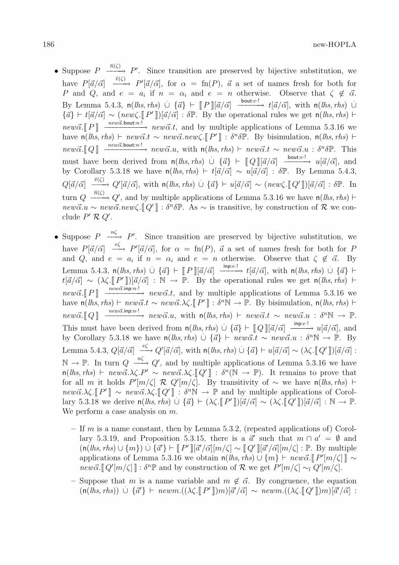
186 new-HOPLA

• Suppose Pn(ζ)−−−−→ P ′. Since transition are preserved by bijective substitution, we

have P [~a/~α]e(ζ)−−−→ P ′[~a/~α], for α = fn(P ), ~a a set of names fresh for both for

P and Q, and e = ai if n = αi and e = n otherwise. Observe that ζ 6∈ ~α.

By Lemma 5.4.3, n(lhs, rhs).∪ {~a} ` JP K[~a/~α]

bout:e·!−−−−−−→ t[~a/~α], with n(lhs, rhs).∪

{~a} ` t[~a/~α] ∼ (newζ.JP ′ K)[~a/~α] : δP. By the operational rules we get n(lhs, rhs) `new~α.JP K

new~α.bout:n·!−−−−−−−−−−→ new~α.t, and by multiple applications of Lemma 5.3.16 wehave n(lhs, rhs) ` new~α.t ∼ new~α.newζ.JP ′ K : δnδP. By bisimulation, n(lhs, rhs) `new~α.JQ K

new~α.bout:n·!−−−−−−−−−−→ new~α.u, with n(lhs, rhs) ` new~α.t ∼ new~α.u : δnδP. This

must have been derived from n(lhs, rhs).∪ {~a} ` JQ K[~a/~α]

bout:e·!−−−−−−→ u[~a/~α], andby Corollary 5.3.18 we have n(lhs, rhs) ` t[~a/~α] ∼ u[~a/~α] : δP. By Lemma 5.4.3,

Q[~a/~α]e(ζ)−−−→ Q′[~a/~α], with n(lhs, rhs)

.∪ {~a} ` u[~a/~α] ∼ (newζ.JQ′ K)[~a/~α] : δP. In

turn Qn(ζ)−−−−→ Q′, and by multiple applications of Lemma 5.3.16 we have n(lhs, rhs) `

new~α.u ∼ new~α.newζ.JQ′ K : δnδP. As ∼ is transitive, by construction of R we con-clude P ′ R Q′.

• Suppose Pnζ−−−→ P ′. Since transition are preserved by bijective substitution, we

have P [~a/~α]eζ−−→ P ′[~a/~α], for α = fn(P ), ~a a set of names fresh for both for P

and Q, and e = ai if n = αi and e = n otherwise. Observe that ζ 6∈ ~α. By

Lemma 5.4.3, n(lhs, rhs).∪ {~a} ` JP K[~a/~α]

inp:e·!−−−−−→ t[~a/~α], with n(lhs, rhs).∪ {~a} `

t[~a/~α] ∼ (λζ.JP ′ K)[~a/~α] : N → P. By the operational rules we get n(lhs, rhs) `new~α.JP K

new~α.inp:n·!−−−−−−−−−→ new~α.t, and by multiple applications of Lemma 5.3.16 wehave n(lhs, rhs) ` new~α.t ∼ new~α.λζ.JP ′ K : δnN → P. By bisimulation, n(lhs, rhs) `new~α.JQ K

new~α.inp:n·!−−−−−−−−−→ new~α.u, with n(lhs, rhs) ` new~α.t ∼ new~α.u : δnN → P.

This must have been derived from n(lhs, rhs).∪ {~a} ` JQ K[~a/~α]

inp:e·!−−−−−→ u[~a/~α], andby Corollary 5.3.18 we have n(lhs, rhs)

.∪ {~a} ` new~α.t ∼ new~α.u : δnN → P. By

Lemma 5.4.3, Q[~a/~α]eζ−−→ Q′[~a/~α], with n(lhs, rhs)

.∪ {~a} ` u[~a/~α] ∼ (λζ.JQ′ K)[~a/~α] :

N → P. In turn Qnζ−−−→ Q′, and by multiple applications of Lemma 5.3.16 we have

n(lhs, rhs) ` new~α.λζ.P ′ ∼ new~α.λζ.JQ′ K : δn(N → P). It remains to prove thatfor all m it holds P ′[m/ζ] R Q′[m/ζ]. By transitivity of ∼ we have n(lhs, rhs) `new~α.λζ.JP ′ K ∼ new~α.λζ.JQ′ K : δnN → P and by multiple applications of Corol-lary 5.3.18 we derive n(lhs, rhs)

.∪ {~a} ` (λζ.JP ′ K)[~a/~α] ∼ (λζ.JQ′ K)[~a/~α] : N → P.

We perform a case analysis on m.

– If m is a name constant, then by Lemma 5.3.2, (repeated applications of) Corol-lary 5.3.19, and Proposition 5.3.15, there is a ~a′ such that m ∩ a′ = ∅ and(n(lhs, rhs) ∪ {m})

.∪ {~a′} ` JP ′ K[~a′/~α][m/ζ] ∼ JQ′ K[~a′/~α][m/ζ] : P. By multiple

applications of Lemma 5.3.16 we obtain n(lhs, rhs) ∪ {m} ` new~α.JP ′[m/ζ] K ∼new~α.JQ′[m/ζ] K : δnP and by construction of R we get P ′[m/ζ] ∼l Q′[m/ζ].

– Suppose that m is a name variable and m 6∈ ~α. By congruence, the equation(n(lhs, rhs))

.∪ {~a′} ` newm.((λζ.JP ′ K)m)[~a′/~α] ∼ newm.((λζ.JQ′ K)m)[~a′/~α] :

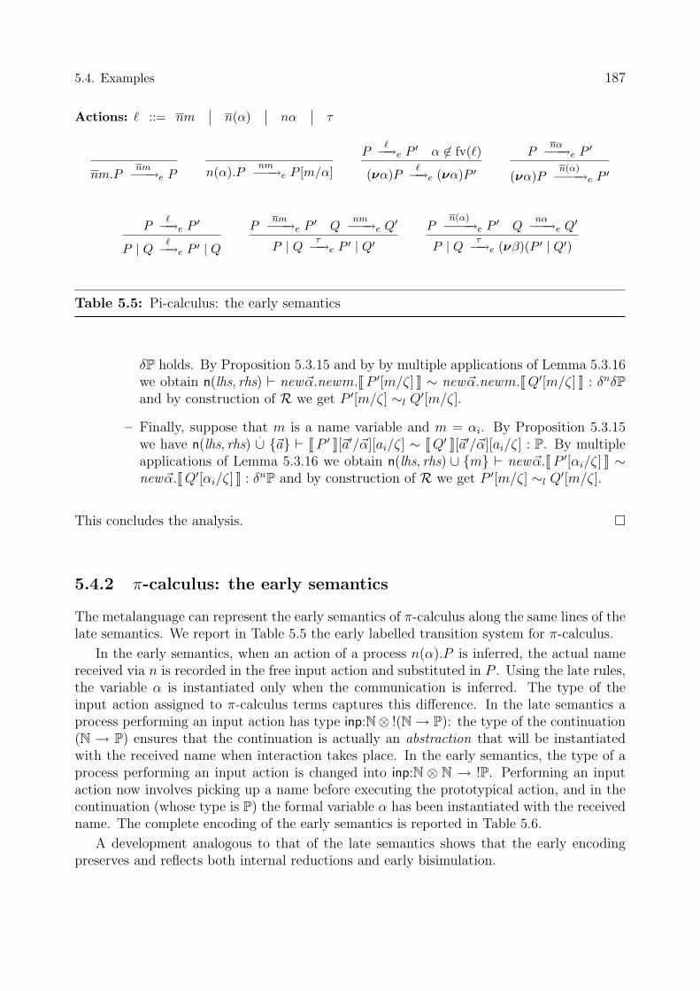
5.4. Examples 187

Actions: ` ::= nm∣∣ n(α)

∣∣ nα∣∣ τ

nm.Pnm−−−→e P n(α).P

nm−−−→e P [m/α]

P`−−→e P ′ α 6∈ fv(`)

(να)P`−−→e (να)P ′

Pnα−−−→e P ′

(να)Pn(α)−−−−→e P ′

P`−−→e P ′

P | Q `−−→e P ′ | Q

Pnm−−−→e P ′ Q

nm−−−→e Q′

P | Q τ−−→e P ′ | Q′

Pn(α)−−−−→e P ′ Q

nα−−−→e Q′

P | Q τ−−→e (νβ)(P ′ | Q′)

Table 5.5: Pi-calculus: the early semantics

δP holds. By Proposition 5.3.15 and by by multiple applications of Lemma 5.3.16we obtain n(lhs, rhs) ` new~α.newm.JP ′[m/ζ] K ∼ new~α.newm.JQ′[m/ζ] K : δnδPand by construction of R we get P ′[m/ζ] ∼l Q′[m/ζ].

– Finally, suppose that m is a name variable and m = αi. By Proposition 5.3.15we have n(lhs, rhs)

.∪ {~a} ` JP ′ K[~a′/~α][ai/ζ] ∼ JQ′ K[~a′/~α][ai/ζ] : P. By multiple

applications of Lemma 5.3.16 we obtain n(lhs, rhs) ∪ {m} ` new~α.JP ′[αi/ζ] K ∼new~α.JQ′[αi/ζ] K : δnP and by construction of R we get P ′[m/ζ] ∼l Q′[m/ζ].

This concludes the analysis. �

5.4.2 π-calculus: the early semantics

The metalanguage can represent the early semantics of π-calculus along the same lines of thelate semantics. We report in Table 5.5 the early labelled transition system for π-calculus.

In the early semantics, when an action of a process n(α).P is inferred, the actual namereceived via n is recorded in the free input action and substituted in P . Using the late rules,the variable α is instantiated only when the communication is inferred. The type of theinput action assigned to π-calculus terms captures this difference. In the late semantics aprocess performing an input action has type inp:N⊗ !(N→ P): the type of the continuation(N → P) ensures that the continuation is actually an abstraction that will be instantiatedwith the received name when interaction takes place. In the early semantics, the type of aprocess performing an input action is changed into inp:N ⊗ N → !P. Performing an inputaction now involves picking up a name before executing the prototypical action, and in thecontinuation (whose type is P) the formal variable α has been instantiated with the receivedname. The complete encoding of the early semantics is reported in Table 5.6.

A development analogous to that of the late semantics shows that the early encodingpreserves and reflects both internal reductions and early bisimulation.

188 new-HOPLA

P = τ :!P + out:N⊗ N⊗ !P + bout:N⊗ !(δP) + inp:N⊗ N→ !P)

J0 K = 0

Jαβ.p K = out:α · β · !J p KJα(β).p K = inp:α · λβ.!J p K)J (να)p K = Res (newα.J p K)

J p | q K = J p K || J q K

Res : δP→ PRes t = [t > newα.τ :!(x[α]))⇒ τ :!Res x]

+ Σβ∈NΣγ∈N[t > newα.out:β · γ · !(x[α])⇒ out:β · γ · !Res x]

+ Σβ∈N[t > newα.out:β · α · !(x[α])⇒ bout:β · !x]

+ Σβ∈N[t > newα.bout:β · !(x[α])⇒ bout:β · !newγ · Res (newη.x[η][γ])]

+ Σβ∈NΣγ∈N[t > newα.inp:β · γ 7→ !(x[α])⇒ inp:β · λγ.!Res (newη.x[η])]

|| : P&P→ Pt || u = [t > τ :!x⇒ τ :!(x || u)]

+ Σβ∈NΣγ∈N[t > out:(β · γ · !x)⇒ [u > inp:(β · γ 7→ !y)⇒ τ :!(x || y)]]

+ Σβ∈N[t > bout:(β · !x)⇒[u > inp:(β · γ 7→ !y)⇒ τ :!Res (newη.(x[η] || (λγ.y)η))]]

+ Σβ∈NΣγ∈N[t > out:β · γ · !x⇒ out:β · γ · !(x || u)]

+ Σβ∈N[t > bout:β · !x⇒ bout:β · !newη.(x[η] || u)]

+ Σβ∈N[t > inp:β · γ 7→ !x⇒ inp:β · λη!((λγ.x)(η) || u)]

+ same cases with t and u swapped.

where η is chosen to avoid clashes with the free name variables of u.

Table 5.6: π-calculus: encoding of the early semantics

5.4. Examples 189

Actions: ` ::= n∣∣ n

∣∣ τ Abstractions: λ~α.P Concretions: (ν~β)〈~m〉P

n~m.Pn−−→ 〈~m〉P n(~α).P

n−−→ λ~α.P

P`−−→ P ′ β 6∈ fv(`)

(νβ)P`−−→ (νβ)P ′

P`−−→ P ′

P | Q `−−→ P ′ | Q

Pn−−→ C Q

n−−→ F

P | Q τ−−→ C • F

where (ν~α)〈~m〉P • λ~β.Q = (να)(P | Q[~m/~β]).

Table 5.7: Polyadic π-calculus: labelled transition system

5.4.3 Polyadic π-calculus

A natural and convenient extension to π-calculus is to admit processes that pass tuplesof names. We present an encoding of the enriched language, the polyadic π-calculus, intonew-HOPLA: polyadicity is a good testing ground for the expressivity of our language.

Writing ~m to denote tuples of names, the terms of polyadic π-calculus are defined by thegrammar below:

P ::= 0∣∣ P | P

∣∣ (να)P∣∣ n~m.P

∣∣ n(~α).P .

We report its semantics in Table 5.7. Standard conventions about abstractions and concre-tions apply (we refer to [Mil91] for a detailed presentation of polyadic π-calculus). We alsoomit symmetric rules.

The type of a polyadic π-calculus process can be defined as:

P = τ :!P + out:N⊗ C + inp:N⊗ !FC = 0:N⊗ C + 1:δC + 2:!PF = 3:N→ F + 4:P

Recursive types are used to encode tuples of (possibly new) names in concretions, and se-quences of name abstractions in abstractions.

The function J− K translates the terms of polyadic π-calculus into new-HOPLA by struc-tural induction, with the help of two simple auxiliary functions, concr and abst, that trans-form a sequence of names and a continuation process into the corresponding concretion or

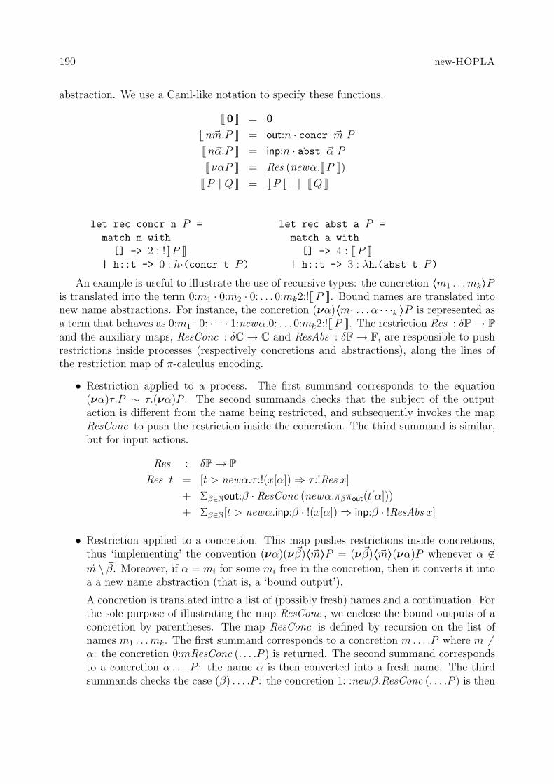
190 new-HOPLA

abstraction. We use a Caml-like notation to specify these functions.

J0 K = 0

Jn~m.P K = out:n · concr ~m P

Jn~α.P K = inp:n · abst ~α P

J ναP K = Res (newα.JP K)JP | Q K = JP K || JQ K

let rec concr n P =

match m with

[] -> 2 : !JP K| h::t -> 0 : h·(concr t P)

let rec abst a P =

match a with

[] -> 4 : JP K| h::t -> 3 : λh.(abst t P)

An example is useful to illustrate the use of recursive types: the concretion 〈m1 . . . mk〉Pis translated into the term 0:m1 · 0:m2 · 0: . . . 0:mk2:!JP K. Bound names are translated intonew name abstractions. For instance, the concretion (να)〈m1 . . . α · · ·k 〉P is represented asa term that behaves as 0:m1 · 0: · · · · 1:newα.0: . . . 0:mk2:!JP K. The restriction Res : δP→ Pand the auxiliary maps, ResConc : δC→ C and ResAbs : δF→ F, are responsible to pushrestrictions inside processes (respectively concretions and abstractions), along the lines ofthe restriction map of π-calculus encoding.

• Restriction applied to a process. The first summand corresponds to the equation(να)τ.P ∼ τ.(να)P . The second summands checks that the subject of the outputaction is different from the name being restricted, and subsequently invokes the mapResConc to push the restriction inside the concretion. The third summand is similar,but for input actions.

Res : δP→ PRes t = [t > newα.τ :!(x[α])⇒ τ :!Res x]

+ Σβ∈Nout:β · ResConc (newα.πβπout(t[α]))

+ Σβ∈N[t > newα.inp:β · !(x[α])⇒ inp:β · !ResAbs x]

• Restriction applied to a concretion. This map pushes restrictions inside concretions,thus ‘implementing’ the convention (να)(ν~β)〈~m〉P = (ν~β)〈~m〉(να)P whenever α 6∈~m \ ~β. Moreover, if α = mi for some mi free in the concretion, then it converts it intoa a new name abstraction (that is, a ‘bound output’).

A concretion is translated intro a list of (possibly fresh) names and a continuation. Forthe sole purpose of illustrating the map ResConc , we enclose the bound outputs of aconcretion by parentheses. The map ResConc is defined by recursion on the list ofnames m1 . . . mk. The first summand corresponds to a concretion m . . . .P where m 6=α: the concretion 0:mResConc (. . . .P ) is returned. The second summand correspondsto a concretion α . . . .P : the name α is then converted into a fresh name. The thirdsummands checks the case (β) . . . .P : the concretion 1: :newβ.ResConc (. . . .P ) is then

5.4. Examples 191

returned. At last, if the concretion is composed by the sole continuation, then the lastrule calls back the Res map to continue pushing the restriction inside the term.

ResConc : δC→ CResConc t = Σγ∈N0:γ · ResConc newα.πγπ0(t[α])

+ 1:newα.παπ0(t[α])

+ 1:newγ.ResConc (newα.((π1(t[α]))[γ]))

+ [t > newα.2:!(x[α])⇒ 2:!Res x]

• Restriction applied to an abstraction. The ResAbs map is defined by recursion on thelist of the abstracted names. It simply pushes the restriction under the λ-abstractions,and if the list of abstractions is empty then calls back the Res map. In other words,it ‘implements’ the convention (να)λ~β.P = λ~β.(να)P .

ResAbs : δF→ FResAbs t = 3:λβ.ResAbs newα.((π3(t[α]))β)

+ Res newα.π4(t[α])

Parallel composition is a family of operations, defined in a simultaneous recursive definitionbelow. For convenience we use infix notation.

• Processes in parallel with processes.

|| : P&P→ Pt || u = Σβ∈N[u > inp:β · !y ⇒ πβπout(t) ||i y]

+ Σβ∈N[u > inp:β.!y ⇒ inp:β · !(t ||a y)]

+ Σβ∈Nout:β · (t ||c πβπout(u))

+ [u > τ :!y ⇒ τ :!(t || y)]

+ symmetric cases

• Concretions in parallel with abstractions. This map implements the application of aconcretion to an abstraction, and corresponds to

(ν~α)〈~m〉P • λ~β.Q = (να)(P | Q[~m/~β]) .

This map is defined by recursion on the length of the list of names ~m.

||i : C&F→ Pt ||i u = π2x || π4y

+ Σβ∈N(πβπ0(x) ||i (π3(y))β)

+ Res newα.((π1(x))[α] ||i (π3(y))α)

192 new-HOPLA

• Concretions in parallel with processes. This map corresponds to the convention

(ν~α)〈~m〉P | Q = (ν~α)〈~m〉(P | Q) for fn(Q) ∩ ~α = ∅ .

||c : C&P→ Ct ||c u = Σβ∈N0:β.((πβπ0(t)) ||c u)

+ 1:newα.(((π1t)[α]) ||c u)

+ [t > 2:!x⇒ 2:!(x || u)]

where α is chosen to avoid clashes with the free name variables of u.

• Abstractions in parallel with processes. This map corresponds to the convention

λ~α.P | Q = λ~α.(P | Q) for fn(Q) ∩ ~α = ∅ .

||a : F&P→ Ft ||a u = 3:λβ.((π3t)β ||a u)

+ 4:((π4t) || u)

where β is chosen to avoid clashes with the free name variables of u.

The encoding preserves and reflects internal reductions of closed terms:

Proposition 5.4.6 Let P be a closed polyadic π-calculus term. If Pτ−−→ P ′, then n(P ) `

JP Kτ :!−−−→∼ JP ′ K. If n(P ) ` JP K

τ :!−−−→ t, then Pτ−−→ P ′ and n(P ) ` t ∼ JP ′ K : P.

We conjecture that late strong bisimilarity is also preserved and reflected by the encoding.

5.4.4 Mobile Ambients

In this section we present an encoding of the mobility core of the Ambient Calculus. Insteadof following the labelled transition system given in Chapter 4, we base our encoding on thesemantics given in [CG96], extending the encoding of Mobile Ambients with public namesinto HOPLA given in [NW02]. As a side effect, we will point out the effects of restrictionon names on the transition of Mobile Ambients.

Again, we denote name constants with a, b, . . ., name variables with α, β, . . ., and we letn, m, . . . range over both name constants and name variables. The terms of the language areconstructed according the following grammar:

P ::= 0∣∣ n[P ]

∣∣ P | P∣∣ (να)P

∣∣ in n.P∣∣ out n.P

∣∣ open n.P .

With respect to the HOPLA encoding, the syntax has been enriched with the restrictionoperator.

5.4. Examples 193

Types for ambients are given recursively by:

P = τ :!P + in:N⊗ !P + out:N⊗ !P + open:N⊗ !P + mvin:N⊗ !C+ mvout:N⊗ !C + open:N⊗ !P + mvın:N⊗ !F

C = 0:P&P + 1:δCF = P→ P

In the HOPLA encoding, the type of concretions was C ::= P&P: it has been changedto reflect that mobility can cause extrusion of names, along the lines of what we did in thelast section for polyadic π-calculus. The injections in, out, and open correspond to the basiccapabilities a process can exercise, while their action on the enclosing ambients is registeredby the components mvin and mvout. The injections open and mvın record the receptiveinteractions that an ambient can (implicitly) have with the environment. Again, recursivetypes are used in concretions to record the sequence of names that must be extruded. 6

The translation of terms is inherited from the HOPLA paper, with the addition of therule for the restriction operator.7

J0 K = 0 J in n.P K = in n · !JP KJn[P ] K = Amb (n, JP K) J out n.P K = out n · !JP K

JP | Q K = JP K || JQ K J open n.P K = open n · !JP KJ (να)P K = Res (newα.JP K)

The restriction map Res : δP → P filters the actions that a process emit, and blocksactions that refer to the name that is restricted. In fact, in Pure Mobile Ambients, the onlyscope extrusions are caused by mobility, and not by pre-actions.

Res : δP→ PRes t = [t > newα.τ :x[α]⇒ τ :Res x)]

+ Σβ∈N[t > newα.in:(β · !x[α])⇒ in:(β · !Res x)]

+ Σβ∈N[t > newα.out:(β · !x[α])⇒ out:(β · !Res x)]

+ Σβ∈N[t > newα.open:(β · !x[α])⇒ open:(β · !Res x)]

+ Σβ∈N[t > newα.mvin:(β · !x[α])⇒ mvin:(β · !1:x)

+ Σβ∈N[t > newα.mvout:(β · !x[α])⇒ mvout:(β · !1:x)

+ Σβ∈N[t > newα.open:(β · !x[α])⇒ open:(β · !Res x)]

+ Σβ∈N[t > newα.mvın:(β · !x[α])⇒ mvın:(β · !λy.Res (newγ.x[γ](y)))]

Parallel composition is a family of operations, one of which is a binary operation betweenprocesses, ||P&P: P&P → P. The family is defined in a simultaneous recursive definitionbelow.

6As a minor notational change, the meaning of actions-coactions mvin,mvın and open, open has beenswapped with respect to the encoding of MA into HOPLA.

7Since the publication of [NW02], the language HOPLA has evolved. In particular the type Σα∈Aα.Pα

has been decomposed into Σα∈APα and !P, and it is definable as Σα∈A!Pα.

194 new-HOPLA

• Processes in parallel with processes:

t || u = Σβ∈N[t > open: β · !x⇒ [u > open: β · !y ⇒ τ :·!(x || y)]]

+ Σβ∈N[t > mvın: β · !f ⇒ [u > mvin: β · !c⇒ τ :·!(c || f)]]

+ [t > τ :!x⇒ τ :!(x || u)]

+ Σβ∈N[t > in:β · !x⇒ in:β · !(x || u)]

+ Σβ∈N[t > out:β · !x⇒ out:β · !(x || u)]

+ Σβ∈N[t > open:β · !x⇒ open:β · !(x || u)]

+ Σβ∈N[t > mvin:β · !x⇒ mvin:β · !(x || u)]

+ Σβ∈N[t > mvout:β · !x⇒ mvout:β · !(x || u)]

+ Σβ∈N[t > open:β · !x⇒ open:β · !(x || u)]

+ Σβ∈N[t > mvın:β · !x⇒ mvın:β · !(x || u)]

+ symmetric cases.

All summands except the first two correspond to congruence rules.

• Concretions in parallel with abstractions:

c ||i f = snd(π0c) || f(fst(π0c)) + Res (newα.(((π1c)[α]) ||i f))

• Concretions in parallel with processes:

c ||c t = 0:(fst(π0c), snd(π0c) || t) + 1:(newα.((π1c)[α] ||c t))

• Abstractions in parallel with processes:

f ||a t = λx.((fx) || u)

Remaining cases are given symmetrically.Finally, ambient creation can be defined recursively in new-HOPLA as an operation

Amb : N&P→ P:

Amb (m, t) = [t > τ :!x⇒ τ :!Amb (m,x)]

+ Σβ∈N[t > in:β · !x⇒ mvin:β · !(Amb (m,x),0)

+ Σβ∈N[t > out:β · !x⇒ mvout:β · !(Amb (m, x),0)

+ [t > mvout:m · !c⇒ τ :!Extr (m, c)]

+ open:m · !t + mvın:m · !λy.Amb (m, t || y)

where the map Extr : N&C→ P extrudes names across ambient’s boundary after an mvoutaction:

Extr(m, c) = fst(π0c) || Amb (m, snd(π0c)) + Res (newα.(Extr (m, (π1c)[α]))) .

Notes and References 195

The denotations of ambients are determined by their capabilities: an ambient m[t] canperform the internal (τ) actions of t, enter a brother ambient (mvin n) if called upon to do soby an in n action of t, exit its parent ambient (mvout n) if called upon to do so by an out naction of t, be exited if t so requests through an mvout m action, be opened (open m), or beentered by an ambient (mvın m); other pre-actions are restricted away. The tree-containmentstructure of ambients is captured in the chain of open m’s that they can perform. The onlydifferences with the rules given in Section 4.2 is that the amb m transition has been split intwo actions open m and mvın m to simplify the types of the continuations.

The semantics given above agrees with the reduction semantics of Mobile Ambients,possibly up to structural congruence:

Proposition 5.4.7

1. If Pτ−−→ Q then n(P ) ` JP K

τ :!−−−→∼ JQ K;

2. if n(P ) ` JP Kτ :!−−−→ t then P

τ−−→ Q for some Q such that n(P ) ` t ∼ JQ K : P.

This propositions relies on the fact that if P ≡ Q, then n(P, Q) ` JP K ∼ JQ K : P. Contraryto what happens in π-calculus and polyadic π-calculus encodings, more name extrusionsthan strictly needed may be performed by τ :! actions. This is because the proposed encodingmakes very difficult to test if given a concretion 〈P 〉Q a name α is free in the process P .

It is easy to prove that if the encodings of two processes are bisimilar in new-HOPLA,then they are strong reduction barbed congruent. We do not know if the converse is true (itis false if we add recursive definition of processes to the fragment of MA we consider). Yet,in MA, strong reduction barbed congruence is an extremely discriminating relation and itsinterest is very limited.

Notes and References

HOPLA and new-HOPLA at a glance The language new-HOPLA extends HOPLAby adding a type of names N, a function space N→ P as well as a type δP supporting newname generation through the abstraction newα.t. Its operational semantics is like that ofHOPLA but given at stages indexed by the current set of names. These extensions makenew-HOPLA much more complex than HOPLA. If a risky parallel can be done, then wefeel that the gap between the two metalanguages is analogous to the gap between CCS andπ-calculus.

Towards a domain theory for concurrency The potentially complicated structure ofcomputation paths suggests building a domain theory directly on computation paths.

This line has been followed also in what seemed originally a different direction: that ofHennessy’s semantics for higher-order processes, in which process equivalence coincides withtesting theories [Hen94].

In Section 5.1 we presented a domain theory based on path sets. Originally, the targetdenotational model of metalanguages such as HOPLA, AL, and new-HOPLA was a moreinformative domain theory than that based on path sets. As remarked earlier, the domainof path sets P, of a path order P, is isomorphic to characteristic functions [Pop,2] orderedpointwise. In modelling a process as a path set we are in effect representing a process bya characteristic function from paths to truth values 0 < 1. If instead of these simple truthvalues we take sets of realisers, replacing 2 by the category of sets Set, we obtain a functorcategory [Pop,Set], whose objects, traditionally called presheaves, provide an alternative‘domain’ of meanings. Viewed as a process, the presheaf X : Pop → Set associates to a pathp ∈ P the set Xp whose elements stand for the ways in which the path can be realised. Asan example, consider the two CCS processes t = a.0 + a.a.0 and u = a.a.0, These processeswill be represented as the same path set, and are thus identified by the path semantics.8

On the other hand, the process t has two different ways of realising the path a0 while uhas only one, and in this way, a presheaf representation will distinguish between the twoprocesses. A presheaf captures the nondeterministic branching of a process and a presheafsemantics can support branching time equivalences. Presheaf models have been proposedfor a wide range of process calculi, including CCS [CW96], higher-order CCS [Cat99], andπ-calculus [CSW97].

More than that, presheaf categories provides a promising framework to develop a domaintheory for concurrency that accounts for independence models, name generation, higher-order processes, and possesses an operational interpretation.

Name generation Behavioural properties of name generation have much in common, atleast intuitively, with that of local variables in Algol-like languages and references in ML-like

8The full abstraction result for HOPLA links path equivalence with simulation equivalence, see [Nyg03].

198 Notes and References

languages.Our denotational model for new-HOPLA is built out of a functor category indexed by

the category I of finite sets and injections. This construction is based on Moggi’s model ofdynamic allocation [Mog90]; it is related to the ‘possible worlds’ models of Reynolds, Tennentand O’Hearn [Rey81, OT91], and also to Mitchell and Moggi’s Kripke-style models [MM91].Crucial ingredients of the dynamic allocation monad used here are the ‘object of names’,given by the inclusion functor I ↪→ Lin, and the shift functor δ : LinI → LinI , given byδP(s) = P(s+1). This approach has been used in [Sta96] and [FMS96] to define denotationalmodels for π-calculus. In these works, the denotational semantics is proved fully abstractwith respect to bisimulation based equivalences. It has been further carried on in [Hen01],where the behavioural preorders are the standard versions of may and must testing adaptedto the π-calculus. Recent work on modelling variable-binding abstract syntax [Hof99, FPT99]is also worth mentioning.

Along a different line, notions of ‘name-abstraction’ and ‘fresh name’ are also supportedby the permutation model of set theory with atoms (FM-sets), devised by Fraenkel andMostowsky in the 1930s [GP01]. FM-sets guided the design of an ML-style metalanguagecalled FreshML [PG00] for programming with bound names modulo renaming.9

Motivations and targets of FreshML and new-HOPLA are different. Their denotationalmodels use unrelated ‘ingredients’ for the allocation monad. Yet, they offer similar syn-tactically constructions to the programmer. In particular FreshML’s atom abstraction andconcretion play roles comparable to those of new-HOPLA’s new name abstraction and newname application. At the same time, FreshML local declaration new a in e end, whoserole is to create a new name and bind it to a in e has no counterpart in new-HOPLA. Infact, the term above has the same type as the expression e, while if we mimic it with newname abstraction, newα.t, the resulting type is δ of the type of t. For people familiar withFreshML, this is why in new-HOPLA patterns cannot be decomposed into atomic patternsmatching only the prototypical action.

9Also visit http://www.freshml.org.

6 Conclusion

In this dissertation we have investigated the semantics of higher-order processes, with theaim to elaborate mathematical tools to express and reason about mobile systems. Behaviouris the unifying concept guiding us all along the different developments.

We focused on two process languages, the Seal Calculus and Mobile Ambients: althoughthey had received a lot of attention from the scientific community, their behavioural theorieswere largely unexplored. We proposed labelled transition semantics, and on top of themwe defined bisimulation based equivalences that are sound proof techniques for reductionbarbed congruence. In MA, the proposed bisimilarity is also complete: this important resultrequired novel techniques to deal with asynchronous mobility, ‘stuttering’ phenomena, andunobservable movements of secret ambients.

A contribution of this thesis is to present a clear picture of the Seal Calculus. We believethat there is not much point in discussing the relative merits of the various collections ofcombinators, as different process languages will be more or less effective depending on thearea of application. Yet, a lesson we learnt is that even if Mobile Ambients behavioural theoryis much more complicated than Seal’s, its syntax and reduction semantics are simpler: thisgreatly simplified its theoretical study.

Some reflections on the LTSs. Technically both Seal bisimilarity and MA bisimilarity arecontextual bisimulations in the sense of [San94]: they solve the contextuality problem by auniversal quantification over all the possible interacting contexts. In Seal we closely followthe approach of [San94]: the universal quantification is part of the definition of bisimulation.As a consequence, the bisimulation must be formulated as a delay bisimulation. In MA,on the contrary, the (essence of the) universal quantification is taken into account by theenv-actions, and is integrated into the LTS. The essence of the interaction with the contextis then captured by the LTS: we believe this presentation favours the emergence of a patternin LTSs for higher-order process calculi. As a side note, a technical contribution of Seal’sLTS is to extend the techniques of [Sew00] to a higher-order LTS. This approach simplifiesthe definition of extrusions of names, though at some cost (in particular it requires workingwith indexed bisimulations).

In the context of MA, we have developed powerful up-to proof methods. In particularbisimulation up to context bisimulation revealed almost indispensable when working with(variants of) context bisimulation. In fact, complex contexts may be introduced in the bisim-ulation game, and without appropriate tools it is awkward to prove even simple properties.The proof of the perfect firewall equation is a startling example.

We have presented a simple domain theory for nondeterministic processes within theframework of Scott and Strachey. An expressive language suitable to describe higher-orderprocesses and name generation is based on canonical constructions on these domains. Wegave an exhaustive presentation of its operational theory. The language has then been usedto give semantics to rich process algebras like π-calculus, polyadic π-calculus, and Mobile

200 Conclusion

Ambients. It is probably too early to summarise the new-HOPLA experience. For instance,we are currently programming an interpreter of new-HOPLA. But the results of this thesismake, we believe, a strong case that the development of the theories underpinning higher-order computation and name generation is truly fundamental.

Further work

This thesis opens several research directions. We briefly outline some of the possibilities.

Our results on the foundations of the Seal Calculus and of Mobile Ambients are step-ping stones not only to investigate more in depth their intrinsic theories, but also in theprogramming practise, to verify that an implementation respects its specification, or thatan abstract machine is correct. One way forward is to refine our techniques to be moresuitable for application specific domains. In particular, we believe that interesting labelledcharacterisations of typed reduction barbed congruence for MA can be derived along thelines of [HMR03].

At the same time, these results are just a contribution towards a reasonably completeunderstanding of higher-order process calculi. Contextual bisimilarity proved a robust toolto define sound bisimulations for higher-order process calculi. The next step is to developtechniques to eliminate, or at least to limit, the universal quantifications over all the in-teracting contexts. The up-to context proof technique goes in this direction, and revealssurprisingly effective. Nevertheless, it would be very satisfying if the LTS we proposed forMA could be extended along the lines of Jeffrey and Rathke approach for HOπ.

A major project is to provide axiomatisations of behavioural equivalences in higher-orderprocess calculi. Even if equational reasoning is a central technique in process calculi, this isa completely unexplored area. Relying on the techniques introduced in Chapter 4, it seemspossible to provide a complete axiomatisation of reduction barbed congruence in Ambient-like calculi. Some steps in this direction have already be undertaken [MZN03a].

The natural continuation of our research on new-HOPLA is to work out the exactrelationships between the language and the denotational model LinI . We expect to obtaina full abstraction result with a natural, linear-time, contextual equivalence characterised asequality of path set denotations. Relating the operational semantics to the more informativedenotational model based on presheaves presents several additional difficulties. In particular,at the time of writing, we do not know whether the function space P→ Q exists in the naturalmodel based on presheaves.

On the operational side, it is unclear how to provide encodings of higher-order processcalculi into new-HOPLA (but the same problem arises with HOPLA) that are fully abstractwith respect to the natural contextual equivalence. In particular, it is unclear how to reconcilethe ideas behind Sangiorgi’s contextual bisimulation with the type-driven bisimulation ofnew-HOPLA. Also, a major inadequacy of the work presented here is the lack of suitableweak equivalences for new-HOPLA. The language new-HOPLA does not have an analogousto internal reductions, so there is the issue of how to support more abstract operationalequivalences. The paper [FCW99] provides a mathematical framework for weak bisimilarityin the context of presheaf models, and might be a good starting point.

Conclusion 201

To conclude this dissertation, we would like to focus on its general scientific project.Our studies of the operational theories of higher-order process languages aimed at a betterunderstanding of the concurrent computation. They were also meant to work towards adomain theory for concurrency which handles higher-order and name generation. Even ifproviding a global mathematical framework for concurrency seems a tall order, we hopethat, on the long term, this line of research will reveal as fruitful as the works of Scott andStrachey for sequential computation.

Bibliography

[ACS98] R. Amadio, I. Castellani, and D. Sangiorgi. On bisimulations for the asynchronousπ-calculus. Theoretical Computer Science, 195:291–324, 1998.

[AGR88] E. Astesiano, A. Giovini, and G. Reggio. Generalized bisimulation in relationalspecifications. In Proc. STACS ’88, volume 294 of LNCS, pages 207–226. SpringerVerlag, 1988.

[AKH92] S. Arun-Kumar and M. Hennessy. An efficiency preorder for processes. ActaInformatica, 29:737–760, 1992.

[BB92] G. Berry and G. Boudol. The chemical abstract machine. Theoretical ComputerScience, 96, 1992.

[BCC01a] M. Bugliesi, G. Castagna, and S. Crafa. Boxed ambients. In Proc. 4th TACS,volume 2215 of LNCS. Springer Verlag, 2001.

[BCC01b] M. Bugliesi, G. Castagna, and S. Crafa. Reasoning about security in mobileambients. In Proc. of 12th CONCUR 2001, LNCS. Springer Verlag, 2001.

[BCMS] M. Bugliesi, S. Crafa, M. Merro, and V. Sassone. Communication interferencein mobile boxed ambients. Forthcoming Technical Report. An extended abstractappeared in Proc. FSTTCS’02, LNCS, Springer Verlag.

[Bou89] G. Boudol. Towards a lambda calculus for concurrent and communicating sys-tems. In Proc. TAPSOFT ’89, volume 351 of LNCS, pages 149–161. SpringerVerlag, 1989.

[Bou92] G. Boudol. Asynchrony and the π-calculus. Technical Report RR-1702, INRIA-Sophia Antipolis, 1992.

[BS98] M. Boreale and D. Sangiorgi. Bisimulation in name-passing calculi withoutmatching. In Proc. 13th LICS. IEEE Computer Society Press, 1998.

[BV01] C. Bryce and J. Vitek. The JavaSeal mobile agent kernel. Autonomous Agentsand Multi-Agent Systems, 4(4):359–384, 2001.

[Cas85] I. Castellani. Bisimulation and abstraction homomorphisms. In Proc. CAAP’85,LNCS. Springer Verlag, 1985.

[Cas01] I. Castellani. Process algebras with localities. In J. Bergstra, A. Ponse, andS. Smolka, editors, Handbook of Process Algebra, pages 945–1045. North-Holland,Amsterdam, 2001.

204 Bibliography

[Cat99] G. L. Cattani. Presheaf models for concurrency. PhD thesis, BRICS, 1999.

[CBC02] S. Crafa, M. Bugliesi, and G. Castagna. Information flow security for BoxedAmbients. In Foundations of Wide Area Network Computing (F-WAN), volume66(3) of ENTCS. Elsevier Science B.V., 2002.

[CG96] L. Cardelli and A. Gordon. A commitment relation for the ambient calculus.Unpublished notes, 1996.

[CG00a] L. Cardelli and A. Gordon. Anytime, anywhere: Modal logics for mobile ambi-ents. In Proc. of the 27th POPL, pages 365–377. ACM Press, 2000.

[CG00b] L. Cardelli and A. Gordon. Mobile ambients. Theoretical Computer Science,240(1):177–213, 2000. An extended abstract appeared in Proc. of FoSSaCS ’98.

[CGZN01] G. Castagna, G. Ghelli, and F. Zappa Nardelli. Typing mobility in the sealcalculus. In Proc. of 12th CONCUR 2001, LNCS. Springer Verlag, 2001.

[CSW97] G. L. Cattani, I. Stark, and G. Winskel. Presheaf models for the π-calculus. InProc. CTCS’97, volume 1290 of LNCS. Springer Verlag, 1997.

[CVZN03] G. Castagna, J. Vitek, and F. Zappa Nardelli. The seal calculus. Manuscript.Available from www.di.ens.fr/~castagna, 2003.

[CW96] G. L. Cattani and G. Winskel. Presheaf models for concurrency. In Proc. CSL’96,volume 1258 of LNCS. Springer Verlag, 1996.

[CW03] G. L. Cattani and G. Winskel. Profunctors, open maps and bisimulation.Manuscript, 2003.

[CZN02] G. Castagna and F. Zappa Nardelli. The seal calculus revisited: Contextualequivalence and bisimilarity. In Proc. 22nd FSTTCS ’02, volume 2556 of LNCS.Springer Verlag, 2002.

[Day70] B. J. Day. On closed categories of functors. In Reports of the Midwest CategorySeminar IV, volume 137 of Lecture Notes in Mathematics, pages 1–38. SpringerVerlag, 1970.

[DH84] R. De Nicola and M. Hennessy. Testing equivalences for processes. TheoreticalComputer Science, 34:83–133, 1984.

[FCW99] M. Fiore, G. L. Cattani, and G Winskel. Weak bisimulation and open maps. InProc. LICS ’99. IEEE Computer Society Press, 1999.

[FG98] C. Fournet and G. Gonthier. A hierarchy of equivalences for asynchronous calculi.In Proc. 25th ICALP, pages 844–855. Springer Verlag, 1998.

Bibliography 205

[FGL+96] C. Fournet, G. Gonthier, J.-J. Levy, L. Maranget, and D. Remy. A calculus of mo-bile processes. In Ugo Montanari and Vladimiro Sassone, editors, CONCUR ’96:Concurrency Theory, 7th International Conference, volume 1119 of LNCS, pages406–421. Springer Verlag, 1996.

[FMS96] M. Fiore, E. Moggi, and D. Sangiorgi. A fully-abstract model for the π-calculus.In Proc. 11th LICS. IEEE Computer Society Press, 1996.

[FMT01] G. Ferrari, U. Montanari, and E. Tuosto. A LTS semantics of ambients via graphsynchronization with mobility. In Proc. ICTCS, volume 2202 of LNCS, 2001.

[Fou98] C. Fournet. The Join-Calculus: a calculus for distributed mobile programming.PhD thesis, Ecole Polytechnique, Paris, 1998.

[FPT99] M. P. Fiore, G. D. Plotkin, and D. Turi. Abstract syntax and variable binding.In Proc. 14th LICS, pages 193–202. IEEE Computer Society Press, 1999.

[GC02] A. D. Gordon and L. Cardelli. Equational properties of mobile ambients. Journalof Mathematical Structures in Computer Science, 12:1–38, 2002. An extendedabstract appeared in Proc. FoSSaCs ’99.

[GHS02] J.C. Godskesen, T. Hildebrandt, and V. Sassone. A calculus of mobile resources.In Proc. 10th CONCUR ’02, volume 2421 of LNCS, 2002.

[Gor95] A. D. Gordon. Bisimilarity as a theory of functional programming: mini-course.Notes Series BRICS-NS-95-3, BRICS, Department of Computer Science, Univer-sity of Aarhus, July 1995.

[GP01] M. J. Gabbay and A. M. Pitts. A new approach to abstract syntax with variablebinding. Formal Aspects of Computing, 2001. A preliminary version appeared inProc. 14th LICS.

[Hen88] M. Hennessy. Algebraic Theory of Processes. The MIT Press, Cambridge, Mass.,1988.

[Hen94] M. Hennessy. A fully abstract denotational model for higher-order processes.Information and Computation, 112(1):55–95, 1994.

[Hen01] M. Hennessy. A fully abstract denotational model for the π-calculus. TheoreticalComputer Science, pages 53–89, 2001.

[HMR03] M. Hennessy, M. Merro, and J. Rathke. Towards a behavioural theory of accessand mobility control in distributed system. In Proc. 5th FoSSaCS ’03, LNCS.Springer Verlag, 2003.

[Hof99] M. Hofmann. Semantical analysis of higher-order abstract syntax. In Proc. 14thLICS, pages 204–213. IEEE Computer Society Press, 1999.

206 Bibliography

[How96] D. J. Howe. Proving congruence of bisimulation in functional programming lan-guages. Information and Computation, 124(2):103–112, 1996.

[HP79] M. Hennessy and G. D. Plotkin. Full abstraction for a simple parallel program-ming language. In Proc. MFCS’79, volume 74 of LNCS. Springer Verlag, 1979.

[HR98] M. Hennessy and J. Riely. A typed language for distributed mobile processes. InProc. 25th POPL. ACM Press, 1998.

[HRY03] M. Hennessy, J. Rathke, and N. Yoshida. Safedpi: a language for controllingmobile code. Computer Science Report 2:03, University of Sussex, 2003.

[HT91] K. Honda and M. Tokoro. An Object Calculus for Asynchronous Communica-tions. In Proc. ECOOP ’91, volume 512 of LNCS. Springer Verlag, 1991.

[HY94] K. Honda and N. Yoshida. Replication in Concurrent Combinators. In Proc.TACS’94, volume 789 of LNCS. Springer Verlag, 1994.

[HY95] K. Honda and N. Yoshida. On reduction-based process semantics. TheoreticalComputer Science, 152(2):437–486, 1995.

[JNW94] A. Joyal, M. Nielsen, and G. Winskel. Bisimulation from open maps. TechnicalReport RS-94-7, BRICS, 1994. An extract in Proc. LICS’93, IEEE ComputerSociety Press.

[JR03] A. Jeffrey and J. Rathke. Contextual equivalence for higher-order π-calculusrevisited. In Proc. MFPS XIX, volume 83 of ENTCS. Elsevier, 2003. Alsoavailable as University of Sussex Computer Science Report 2002:04.

[LS00a] F. Levi and D. Sangiorgi. Controlling interference in ambients. In Proc. 27thPOPL. ACM Press, 2000.

[LS00b] F. Levi and D. Sangiorgi. Controlling interference in ambients. An extendedabstract appeared in Proc. 27th Symposium on Principles of Programming Lan-guages, ACM Press, 2000.

[LW84] K. G. Larsen and G. Winskel. Using informations systems to solve recursivedomain equations effectively. In Proc. Semantics of Data Types, volume 173 ofLNCS. Springer Verlag, 1984.

[MH01] M. Merro and M. Hennessy. Bisimulation congruences in safe ambients. ComputerScience Report 5/01, University of Sussex, 2001.

[MH02] M. Merro and M. Hennessy. Bisimulation congruences in safe ambients. In Proc.29th POPL ’02. ACM Press, 2002.

[Mil89] R. Milner. Communication and Concurrency. Prentice Hall, 1989.

Bibliography 207

[Mil91] R. Milner. The polyadic π-calculus: a tutorial. Technical Report ECS–LFCS–91–180, LFCS, Dept. of Comp. Sci., Edinburgh Univ., October 1991. Also in Logicand Algebra of Specification, ed. F.L. Bauer, W. Brauer and H. Schwichtenberg,Springer Verlag, 1993.

[MM91] J. C. Mitchell and E. Moggi. Kripke-style models for typed lambda calculus.Annals of Pure and Applied Logic, 51:99–124, 1991.

[Mog90] E. Moggi. An abstract view of programming languages. Technical Report ECS-LFCS-90-113, LFCS, Dept. of Comp. Sci., Edinburgh Univ., 1990.

[MPW92] R. Milner, J. Parrow, and D. Walker. A calculus of mobile processes, (Parts Iand II). Information and Computation, 100:1–77, 1992.

[MS92] R. Milner and D. Sangiorgi. Barbed bisimulation. In Proc. 19th ICALP, volume623 of LNCS, pages 685–695. Springer Verlag, 1992.

[MZN03a] M. Merro and F. Zappa Nardelli. Axioms for safe ambients. Manuscript, 2003.

[MZN03b] M. Merro and F. Zappa Nardelli. Bisimulation proof methods for mobileambients. In Proc. ICALP 2003. Springer Verlag, 2003. An extended ver-sion is available as Computer Science Report 2003:01, University of Sussex,http://cogslib.cogs.susx.ac.uk/csr abs.php?cs.

[NPW81] M. Nielsen, G. Plotkin, and G. Winskel. Petri nets, event structures and domains,part I. Theoretical Computer Science, 13(1):85–108, 1981.

[NW] M. Nygaard and G. Winskel. Domain theory for concurrency. To appear inTheoretical Computer Science, special issue on domain theory.

[NW02] M. Nygaard and G. Winskel. Hopla—a higher-order process language. In Proc.CONCUR’02, volume 2421 of LNCS. Springer Verlag, 2002.

[NW03] M. Nygaard and G. Winskel. Full abstraction for HOPLA. In Proc. CONCUR’03,LNCS. Springer Verlag, 2003.

[Nyg03] M. Nygaard. Domain theory for concurrency. PhD thesis, BRICS, 2003.

[OT91] P. W. O’Hearn and R. D. Tennent. Semantics of local variables. In Applicationsof categories in computer science, number 177 in London Mathematical SocietyLecture Note Series, pages 217–238. CUP, 1991.

[Par81] D.M. Park. Concurrency on automata and infinite sequences. In P. Deussen,editor, Conf. on Theoretical Computer Science, volume 104 of LNCS. SpringerVerlag, 1981.

[PG00] A. M. Pitts and M. J. Gabbay. A metalanguage for programming with boundnames modulo renaming. In Proc. MPC 2000, volume 1837 of LNCS. SpringerVerlag, 2000.

208 Bibliography

[Pit97] A. M. Pitts. Operationally-based theories of program equivalence. In P. Dybjerand A. M. Pitts, editors, Semantics and Logics of Computation, Publications ofthe Newton Institute, pages 241–298. Cambridge University Press, 1997.

[PJ03] Sewell P. and Vitek J. Composition of untrusted code: Wrappers and causalitytypes. Journal of Computer Security, 2003.

[PS00] B. Pierce and D. Sangiorgi. Behavioral equivalence in the polymorphic pi-calculus. Journal of the ACM, 47(3):531–584, 2000.

[Rey81] J. C. Reynolds. The essence of Algol. In Proc. 1981 International Symposyoumon Algorithmic Languages, pages 345–372. North Holland, 1981.

[RH97] J. Riely and M. Hennessy. Distributed processes and location failures. In Proc.ICALP ’97, volume 1256 of LNCS. Springer Verlag, 1997.

[San92] D. Sangiorgi. Expressing Mobility in Process Algebras: First-Order and Higher-Order Paradigms. PhD thesis CST–99–93, Dept. of Comp. Sci., Edinburgh Univ.,1992.

[San94] D. Sangiorgi. Bisimulation in higher-order calculi. In Proc. IFIP Working Confer-ence on Programming Concepts, Methods and Calculi (PROCOMET’94), pages207–224. North-Holland, 1994.

[San96a] D. Sangiorgi. Bisimulation for Higher-Order Process Calculi. Information andComputation, 131(2):141–178, 1996.

[San96b] D. Sangiorgi. Locality and non-interleaving semantics in calculi for mobile pro-cesses. Theoretical Computer Science, 155:39–83, 1996.

[San98] D. Sangiorgi. On the bisimulation proof method. Journal of Mathematical Struc-tures in Computer Science, 8:447–479, 1998.

[San01] D. Sangiorgi. Extensionality and intensionality of the ambient logic. In Proc.28th POPL. ACM Press, 2001.

[Sco82] D. S. Scott. Domains for denotational semantics. In Proc. ICALP’82, volume140 of LNCS. Springer Verlag, 1982.

[Sew00] P. Sewell. Applied π – a brief tutorial. Technical Report 498, Computer Labora-tory, University of Cambridge, 2000.

[Sew03] P. Sewell. From rewrite rules to bisimulation congruences. TCS, 2003. To appear.

[SM92] D. Sangiorgi and R. Milner. The problem of “Weak Bisimulation up to”. In Proc.CONCUR ’92, volume 630 of LNCS, pages 32–46. Springer Verlag, 1992.

[Sta96] I. Stark. A fully-abstract domain model for the π-calculus. In Proc. 11th LICS,pages 36–42, Washington, DC, 1996. IEE Computer Society Press.

Bibliography 209

[SV99] P. Sewell and J. Vitek. Secure composition of insecure components. In 12th IEEEComputer Security Foundations Workshop, 1999.

[SW01] D. Sangiorgi and D. Walker. The π-calculus: a Theory of Mobile Processes.Cambridge University Press, 2001.

[Tho90] B. Thomsen. Calculi for Higher Order Communicating Systems. PhD thesis,Department of Computing, Imperial College, 1990.

[VC99] J. Vitek and G. Castagna. Seal: A framework for secure mobile computations. InInternet Programming Languages, number 1686 in LNCS, pages 47–77. SpringerVerlag, 1999.

[Vig99] M. G. Vigliotti. Transition systems for the ambient calculus. Master thesis,Imperial College of Science, Technology and Medicine (University of London),September 1999.

[WN95] G. Winskel and M. Nielsen. Models for concurrency. In S. Abramsky et al.,editors, Handbook of Logic in Computer Science. Volume 4. Semantic modelling.Oxford University Press, 1995.

[WZN03] G. Winskel and F. Zappa Nardelli. Name generation and higher-order processes.Manuscript, 2003.

[ZN00] F. Zappa Nardelli. Types for the seal calculus. Master’s thesis, Universita diPisa, 2000.

[ZN03] F. Zappa Nardelli. Notes on ‘very early’ transitions in mobile ambients.Manuscript. Available from www.di.ens.fr/~zappa/EarlyPtma.ps.gz, 2003.

Resume : La presente these etudie les theories a la base de la mobilite, dans le but de developperdes outils mathematiques de formalisation et de preuve des proprietes des systemes mobiles.Afin de comprendre l’impact de la mobilite sur la theorie equationelle des langages, nous noussommes interesse a deux calculs de processus presentant deux modeles de mobilite opposes : le SealCalcul et les Ambients Mobiles. Dans les deux cas, nous avons donne une bisimulation etiquetee quicaracterise l’equivalence observationnelle, ce qui a permis non seulement de developper des tech-niques puissantes de preuves de l’equivalence de deux systemes, mais a aussi mis en relief certainesspecificites des deux modeles de mobilite. Dans le cas des Ambients Mobiles, la caracterisation estcomplete : ce resultat important a necessite l’elaboration de techniques specifiques permettant demanipuler la mobilite asynchrone et le stuttering. De plus, pour la premiere fois dans le cas decalculs d’ordre superieur, on a demontre que des techniques de preuve dites up-to sont correctes.En parallele, nous avons pris les categories de pre-faisceaux comme modele de la concurrence,et nous avons donne une lecture operationnelle d’une categorie de pre-faisceaux appropriee pourmodeliser la creation de noms et les processus d’ordre superieur. Cela nous a conduit a la definitiond’un langage concis mais expressif, nomme new-HOPLA, a meme de representer une grande varietede langages de processus. Le langage est type, et le type d’un terme decrit la forme des cheminsd’execution qu’il peut realiser. Il a donc fallu elaborer le typage du langage, ce qui a ete compliquepar la necessite de distinguer les noms inedits des autres, ainsi que sa theorie operationnelle. Nousavons en outre montre comment new-HOPLA peut etre utilise pour donner une semantique a descalculs de processus comme le π-calcul et les Ambients Mobiles.

Summary: This PhD dissertation addresses the theories underlying the mobile computation, withthe aim to develop mathematical tools to express and reason about mobile systems.We studied the impact that mobility of active computations has on the observational congruence,and in general on the equational theory of a process language. In particular, we focused on twoprocess calculi, namely the Seal Calculus and the Ambient Calculus, that offer two opposite modelsof mobile computation. In both cases, we found a coinductive characterisation of observationalcongruence: these results not only originate powerful proof methods to prove the equivalenceof two systems, but also highlight peculiarities of the two models of mobility. In the case of theAmbient Calculus, the characterisation is complete: this important result required the developmentof techniques to deal with asynchronous mobility and “stuttering” phenomena. Also, we showedthe soundness of up-to proof techniques in the presence of higher-order computation.We also studied presheaf categories as a general model of concurrency. We gave an operationalreading of a presheaf category suitable to describe higher-order process and name generation. Thisled us to a compact but expressive language, called new-HOPLA, that directly encodes a richvariety of process languages. The language is typed, and the type of a term describes the shapeof the computation paths it can perform. The operational theory of the metalanguage and theresulting operational equivalence have been investigated. The metalanguage has been used to givesemantics to rich process algebras like π-calculus and Mobile Ambients.

Discipline : Informatique

Mots-cles : Informatique theorique, semantique de la concurrence, processus d’ordre superieur,equivalence comportementale, bisimulation, typage

Adresse : Departement d’informatique, Ecole normale superieure, 45 rue d’Ulm, 75005 Paris