university of brasÍlia

USING MACHINE LEARNING TO PREDICT

ACTIVITY CHAINS AND MODE CHOICE ON

TRANSPORTATION MODELS

DANIELE FIRME MIRANDA

MASTER’S THESIS IN TRANSPORTATION

DEPARTMENT OF CIVIL AND ENVIRONMENTAL ENGINEERING

FACULTY OF TECHNOLOGY

UNIVERSITY OF BRASÍLIA




USING MACHINE LEARNING TO PREDICT ACTIVITY

CHAINS AND MODE CHOICE ON TRANSPORTATION

MODELS


ADVISOR: PASTOR WILLY GONZALES TACO

MASTER’S THESIS IN TRANSPORTATION

PUBLICATION: T.DM-006/2020

BRASÍLIA/DF: OCTOBER/2020

ii




USING MACHINE LEARNING TO PREDICT ACTIVITY CHAINS AND

MODE CHOICE ON TRANSPORTATION MODELS


MASTER'S THESIS SUBMITTED TO THE GRADUATE PROGRAM IN

TRANSPORTATION OF THE DEPARTMENT OF CIVIL AND ENVIRONMENTAL

ENGINEERING OF THE FACULTY OF TECHNOLOGY, AT THE UNIVERSITY OF

BRASÍLIA, AS PART OF THE REQUIREMENTS TO OBTAIN THE MASTER'S

DEGREE IN TRANSPORTATION.

APROOVED BY:

_________________________________________

PASTOR WILLY GONZALES TACO, DR. (UnB)

(ADVISOR)

_________________________________________

ALAN RICARDO DA SILVA, DR, (UnB)

(INTERNAL EXAMINER)

_________________________________________

CIRA SOUZA PITOMBO, DRA, (USP)

(EXTERNAL EXAMINER)

BRASÍLIA/DF, 26th of October, 2020.

iii

CATALOG FORM

REFERENCE (Example in Brazilian Portuguese)

MIRANDA, D. F. (2020). Using machine learning to predict activity chains and mode choice

on transportation models. Publicação T.DM-006/2020. Departamento de Engenharia Civil e

Ambiental, Universidade de Brasília, Brasília, DF, 96 p.

COPYRIGHT

AUTHOR: Daniele Firme Miranda

THESIS TITLE: Using machine learning to predict activity chains and mode choice on

transportation models.

DEGREE: Mestre/Master YEAR: 2020

Permission is granted to the University of Brasília to reproduce copies of this master’s thesis

and to lend or sell such copies for academic and scientific purposes only. The author reserves

other publishing rights and no part of this master’s thesis may be reproduced without written

authorization from the author.

___________________________

Daniele Firme Miranda

MIRANDA, DANIELE FIRME

Using Machine Learning to Predict Activity Chains and Mode Choice on

Transportation Models. Brasília, 2020.

xiii, 96p., 210x297mm (ENC/FT/UnB, Master, Transportation, 2020).

Master’s Thesis – University of Brasília. Faculty of Technology. Department of

Civil and Environmental Engineering.

1 – Transport modeling 2 – Machine learning

3 – Activity-based 4 – Mode choice

I – ENC/FT/UnB II – Título (série)

iv

“It seems to me that when it’s time to die, there would be

a certain pleasure in thinking that you had utilized your

life well, learned as much as you could, gathered in as

much as possible of the universe, and enjoyed it.”

- Isaac Asimov

v

AGRADECIMENTOS

Agradeço primeiramente ao meu orientador, o professor Pastor Taco, pela sabedoria transmitida

ao longo desses quase dois anos de orientação, por sempre apoiar as minhas ideias e por ter

muita paciência em me colocar no caminho correto da pesquisa.

À professora Fabiana, agradeço por ainda na época da graduação ter me apresentado não só o

mundo dos transportes, mas também o belíssimo caminho da ciência.

Agradeço aos demais professores do PPGT que me acompanharam nas disciplinas,

principalmente à professora Michelle e ao professor Alan, cujas aulas me acrescentaram muito.

Deixo meu agradecimento também a Camila, que na secretaria estava sempre nos ajudando com

a burocracia do dia-a-dia.

Aos meus colegas do mestrado e do Grupo de Pesquisa Comportamento em Transportes e

Novas Tecnologias, agradeço pela parceria nos trabalhos que desenvolvemos juntos. Um

agradecimento especial a Lorena por ter enriquecido imensamente nosso trabalho com o

MATSim.

Agradeço à minha amiga Jéssica por ouvir meus desabafos da rotina dividida entre trabalho e

mestrado e por me ajudar a colocar os pés no chão nos momentos de desespero.

Aos meus pais, Élvis e Veneza, agradeço por terem dedicado suas vidas para proporcionar as

melhores oportunidades para mim e para o meu irmão. Esse título de Mestre eu dedico a vocês,

e prometo continuar em busca de conquistas ainda maiores.

Ao meu irmãozinho Élvis Júnior, agradeço por me inspirar a ser uma pessoa mais tranquila e a

levar a vida com mais leveza.

Agradeço ao meu querido Bruno por me lembrar sempre de que a vida é boa e por acreditar

mais em mim do que eu mesma acredito. Agradeço pelo companheirismo nessa jornada e estou

ansiosa por todas as aventuras que ainda viveremos juntos.

vi

ABSTRACT

When travel is considered a demand derived from people’s need to perform activities, it

becomes clear that a better understanding of how people organize their activities during a day

must provide a more solid basis for travel demand modeling. By replicating disaggregate travel

decisions (at the individual level), activity-based models may produce better travel demand

predictions, compared to the previous generations of modeling approaches (trip-based

approaches, for instance). A paper published in 2019 stands out among the most recent activity-

based modeling research as the authors propose a comprehensive framework for generating full

and detailed activity schedules for given agents depending on their sociodemographic features,

called Data-Driven Activity Scheduler (DDAS).

The aim of this research was to develop a commented replication of the methodological

approach of two modules of the DDAS: the Activity Type Model (ATM) and the Mode Choice

Model (MCM). Specific objectives included replicating these two modules of the DDAS

framework using data from the Federal District Urban Mobility Survey, which is significantly

larger than the dataset used in the original DDAS study. Moreover, it was intended to

investigate possible improvements to be made on the DDAS framework, including its validation

procedure.

The obtained results from the replication of the DDAS framework indicated that there was

improvement to be made on the manner how models were being trained, in order to better deal

with class imbalance. Therefore, a second implementation was made by using the SMOTE

technique (Synthetic Minority Oversampling Technique) for training the ATM and MCM

modules. Although activity chains seemed more realistic in this second set of results, the overall

validation score for the ATM module was low. Therefore, a third model was developed by

training the models as Random Forest classifiers instead of isolated Decision Tree classifiers

as it was defined in the original DDAS framework. Significant improvement was observed in

the results of this third model, both in training and test, for both ATM and MCM modules.

Furthermore, another contribution of this study is the public availability of all scripts that were

developed during its conduction.

vii

RESUMO

Considerando as viagens como demanda derivada da necessidade das pessoas de executar suas

atividades, fica claro que um melhor entendimento de como as pessoas organizam essas

atividades durante o dia leva a uma modelagem de demanda por transportes mais sólida.

Replicando decisões desagregadas (individuais) de transporte, os modelos baseados em

atividades podem produzir melhores previsões de demanda por viagens comparados às gerações

anteriores de abordagens de modelagem (a modelagem baseada em viagens, por exemplo). Um

artigo publicado em 2019 se destaca entre as produções científicas recentes relacionadas à

modelagem baseada em atividades por propor um modelo composto para geração de diários

detalhados de atividades para agentes, com base em suas características socioeconômicas, o

Agendador de Atividades Baseado em Dados (Data-Driven Activity Scheduler – DDAS).

O objetivo deste trabalho foi desenvolver uma replicação comentada da abordagem

metodológica de dois módulos do DDAS: o Modelo de Tipo de Atividade (Activity Type Model

– ATM) e o Modelo de Escolha Modal (Mode Choice Model – MCM). Objetivos específicos

incluíam a replicação destes módulos do DDAS usando dados da Pesquisa de Mobilidade

Urbana do Distrito Federal, que é significativamente maior que a base de dados utilizada no

artigo original. Além disso, pretendia-se investigar possíveis melhorias a serem feitas aos

modelos do DDAS ou ao seu método de validação.

Os resultados obtidos indicaram que uma modificação no método de treino dos modelos poderia

compensar o desbalanço de frequência entre as classes. Assim, foi desenvolvida uma segunda

implementação usando a técnica de SMOTE (Synthetic Minority Oversampling Technique –

Técnica de Sobreamostragem Sintética de Minoria) para treinar os módulos ATM e MCM.

Apesar de terem sido obtidas cadeias de atividades mais realistas a partir dessa segunda

implementação, o score de validação para o módulo ATM foi baixo. Dessa forma, uma terceira

implementação foi desenvolvida, com os modelos treinados como classificadores Random

Forest no lugar de classificadores de árvore de decisão isoladas. Foi observada melhoria

significativa nos resultados desse terceiro modelo, tanto no treinamento quanto na validação,

para ambos os módulos ATM e MCM. Além disso, outra contribuição desse trabalho foi a

disponibilização pública de todos os códigos desenvolvidos durante sua condução.

viii

CONTENTS

1 INTRODUCTION ............................................................................................................ 1

1.1 BACKGROUND AND CONTEXT ............................................................................ 1

1.2 OBJECTIVES .............................................................................................................. 3

1.3 JUSTIFICATION ........................................................................................................ 3

1.4 METHODOLOGICAL DESIGN OF THIS RESEARCH .......................................... 4

2 LITERATURE REVIEW ................................................................................................ 5

2.1 ACTIVITY-BASED TRAVEL DEMAND MODELING .......................................... 5

2.2 KEY CONCEPTS IN MACHINE LEARNING ......................................................... 6

2.2.1 Decision Tree Classifiers ..................................................................................... 6

2.2.2 Random Forest Classifiers ................................................................................... 9

2.2.3 Metrics for evaluating classifiers ....................................................................... 10

2.3 MACHINE LEARNING AND ACTIVITY BASED MODELS .............................. 14

2.3.1 Existing literature review on machine learning and ABM ................................. 14

2.3.2 Complementary review on machine learning and ABM .................................... 16

2.4 RESEARCH ON ACTIVITY-BASED MODELING IN PORTUGUESE ............... 18

2.4.1 Review approach ................................................................................................ 18

2.4.2 Query results and analysis .................................................................................. 19

2.5 CONCLUSIONS OF THE CHAPTER ..................................................................... 20

3 METHOD ........................................................................................................................ 21

3.1 THE DATA-DRIVEN ACTIVITY SCHEDULER .................................................. 21

3.1.1 Algorithm design considerations ........................................................................ 21

3.1.2 Required dataset ................................................................................................. 22

3.2 VALIDATION FRAMEWORK ............................................................................... 23

3.2.1 Generalities ......................................................................................................... 23

3.2.2 Activity count validation .................................................................................... 23

3.2.3 Travel mode choice validation ........................................................................... 23

3.3 DATA DESCRIPTION AND PREPARATION ....................................................... 24

3.3.1 Available dataset ................................................................................................ 24

3.3.2 Obtaining and organizing the socio-demography (soc) dataset ......................... 27

3.3.3 Obtaining and organizing the reach dataset ....................................................... 29

3.3.4 Obtaining and organizing travel information ..................................................... 31

3.3.5 Converting feature types .................................................................................... 33

3.3.6 Profiling the organized dataset ........................................................................... 34

3.4 MODEL TRAINING AND TESTING ..................................................................... 36

3.4.1 The original DDAS framework .......................................................................... 36

ix

4 RESULTS AND ANALYSIS ......................................................................................... 39

4.1 MODEL 1: THE ORIGINAL DDAS FRAMEWORK ............................................. 39

4.1.1 Training results for Model 1 ............................................................................... 39

4.1.2 Test results for Model 1: general ........................................................................ 44

4.1.3 Test results for Model 1: ATM module ............................................................. 44

4.1.4 Test results for Model 1: MCM module............................................................. 49

4.1.5 Partial conclusions after implementing Model 1 ................................................ 51

4.2 MODEL 2: IMPROVING THE DECISION TREE CLASSIFIER .......................... 51

4.2.1 Changing the score function for Model 1........................................................... 51

4.2.2 Training Model 2 using the SMOTE technique ................................................. 53





4.3 MODEL 3: USING A RANDOM FOREST CLASSIFIER ...................................... 63

4.3.1 Training results for Model 3 ............................................................................... 63





4.4 SUMMARY OF RESULTS ...................................................................................... 72

5 CONCLUSIONS AND RECOMMENDATIONS ....................................................... 74

5.1 CONCLUSIONS ....................................................................................................... 74

5.2 LIMITATIONS OF THE STUDY ............................................................................ 76

5.3 RECOMMENDATIONS FOR FUTURE RESEARCH ........................................... 77

REFERENCES ....................................................................................................................... 78

APPENDIX A: Results of the Complementary Literature Review ................................... 90

APPENDIX B: Results for the Brazilian Literature Review ............................................. 93

APPENDIX C: Procedure for Creating Distance Matrices ............................................... 95

APPENDIX D: Code for implementing the Method Described in this Document........... 96

x

LIST OF TABLES

Table 2.1: Characteristics of econometric activity-based models and computational based

activity scheduling models (HAFEZI et al., 2018). ................................................................... 5 Table 2.2: Literature about ML applications for ABM, extracted from the review by Koushik

et al. (2020), classified by machine learning algorithm (rows) and applications (columns). .. 15 Table 2.3: Search terms and number of results for queries on both Scopus and Web of Science.

.................................................................................................................................................. 17

Table 2.4: Search terms and number of results for queries on the Brazilian Catalog of Ph.D.

Dissertations and Master’s Thesis. ........................................................................................... 19 Table 3.1: Features of the organized soc dataset. ..................................................................... 28 Table 3.2: Correspondence between activity types on the organized dataset and on the FDUMS

dataset, and respective frequencies .......................................................................................... 32 Table 3.3: Correspondence between mode types on the organized dataset and on the FDUMS

dataset, and respective frequencies .......................................................................................... 32

Table 4.1: F1-scores for training the ATM and MCM modules of Model 1, compared to the

results presented by Drchal et al. (2019), which is DDAS original implementation. .............. 40 Table 4.2: Score metrics for a cross-validation set of the ATM module, adopting the optimal

tree depth that was previously found (depth = 6). .................................................................... 42

Table 4.3: Score metrics for a cross-validation set of the MCM module, adopting the optimal

tree depth that was previously found (depth = 10). .................................................................. 43

Table 4.4: Expected and observed frequency of activity chains for Model 1. ......................... 45 Table 4.5: Permutation importance for features of the ATM module in Model 1. .................. 47 Table 4.6: Balanced accuracy scores for training the ATM and MCM modules of Model 1. . 53

Table 4.7: Balanced accuracy scores for training the ATM and MCM modules of Model 2,

compared to the results obtained on Model 1. ......................................................................... 54

Table 4.8: Expected and observed frequency of activity chains for Model 2. ......................... 56 Table 4.9: Permutation importance for features of the ATM module in Models 1 and 2. ....... 58

Table 4.10: Comparison between chi-square values computed for each class on the activity type

validation for both Models 1 and 2 (values in bold indicate better measures). ........................ 60 Table 4.11: Comparison between chi-square values computed for each class on the mode type

validation for both Models 1 and 2 (values in bold indicate better measures). ........................ 62


compared to the results obtained on Models 1 and 2. .............................................................. 64 Table 4.13: Expected and observed frequency of activity chains for Model 3. ....................... 66 Table 4.14: Permutation importance for features of the ATM module in Models 1, 2 and 3. . 68

Table 4.15: Comparison between chi-square values computed for each class on the activity type

validation for Models 1, 2 and 3 (values in bold indicate better measures). ............................ 69 Table 4.16: Comparison between chi-square values computed for each class on the travel mode

choice validation for Models 1, 2 and 3 (values in bold indicate better measures). ................ 72 Table 4.17: Summary of the results of the current study. ........................................................ 72

xi

LIST OF FIGURES

Figure 1.1: Methodological design of this research. .................................................................. 4 Figure 2.1: Graphical example of a hypothetical decision tree algorithm. ................................ 6 Figure 2.2: Pseudo-code of a generic decision tree algorithm (KOTSIANTIS, 2007). ............. 7 Figure 2.3: Confusion matrix for a hypothetical travel mode choice prediction task. ............. 11

Figure 2.4: Comparison between evaluation metrics based on two hypothetical travel mode

choice classification task. ......................................................................................................... 14 Figure 3.1: Agent’s elements, schedule composition and activities’ features. ........................ 21 Figure 3.2: Spatial scope of the FDUMS survey. .................................................................... 25 Figure 3.3: Example of a trip duration matrix. ......................................................................... 29

Figure 3.4: Example of the one-hot encoding (OHE) process. ................................................ 34 Figure 3.5: Profile of the “gender” feature on both the original and the clean datasets. ......... 34

Figure 3.6: Profile of the “age” feature on both the original and the clean datasets. ............... 35 Figure 3.7: Profile of the “education_achieved” feature on both the original and the clean

datasets. .................................................................................................................................... 36 Figure 4.1: Selection of ATM tree depth via cross-validation for Model 1, ............................ 40 Figure 4.2: Selection of MCM tree depth via cross-validation for Model 1, ........................... 40

Figure 4.3: Confusion matrix for a cross-validation set of the ATM module, adopting the

optimal tree depth that was previously found (depth = 6)........................................................ 42

Figure 4.4: Confusion matrix for a cross-validation set of the MCM module, adopting the

optimal tree depth that was previously found (depth = 10)...................................................... 43

Figure 4.5: Comparison between the expected and observed proportions of activity types on the

agent’s schedules, for Model 1. ................................................................................................ 45 Figure 4.6: Activity count validation for Model 1. .................................................................. 48

Figure 4.7: Travel mode choice validation for Model 1. ......................................................... 50

Figure 4.8: Selection of ATM tree depth via cross-validation, for Model 1, ........................... 52 Figure 4.9: Selection of MCM tree depth via cross-validation, for Model 1, .......................... 52 Figure 4.10: Selection of ATM tree depth via cross-validation, for Model 2, using the SMOTE

technique, balanced-accuracy vs. tree depth. ........................................................................... 54 Figure 4.11: Selection of MCM tree depth via cross-validation, for Model 2, using the SMOTE

technique, balanced-accuracy vs. tree depth. ........................................................................... 54 Figure 4.12: Comparison between the expected and observed proportions (Models 1 and 2) of

activity types on the agent’s schedules. ................................................................................... 55

Figure 4.13: Comparison between expected chain lengths and results obtained from Model 2.

.................................................................................................................................................. 57

Figure 4.14: Activity count validation for Model 2. ................................................................ 60

Figure 4.15: Travel mode choice validation for Model 2. ....................................................... 61

Figure 4.16: Selection of ATM tree depth for the Random Forest Classifier via cross-validation

for Model 3, balanced accuracy vs. tree depth. ........................................................................ 64 Figure 4.17: Selection of MCM tree depth for the Random Forest Classifier via cross-validation

for Model 3, balanced accuracy vs. tree depth. ........................................................................ 64 Figure 4.18: Comparison between the expected and observed proportions (Models 1, 2 and 3)

of activity types on the agent’s schedules. ............................................................................... 66 Figure 4.19: Comparison between expected chain lengths and results obtained from Model 3.

.................................................................................................................................................. 67 Figure 4.20: Activity count validation for Model 3. ................................................................ 69 Figure 4.21: Travel mode choice validation for Model 3. ....................................................... 71

xii

LIST OF SYMBOLS, NAMES AND ABREVIATIONS

ABM Activity-Based Model/Modeling

ATM Activity Type Model

AR Administrative Region

MCM Mode Choice Model

ML Machine Learning

1

1 INTRODUCTION

1.1 BACKGROUND AND CONTEXT

Cascetta (2009) defines a travel-demand model as a mathematical relationship between travel-

demand flows and agents (and their characteristics) and activity and transportation supply

systems (and their characteristics). The review presented by Hafezi et al. (2018) describes the

major generations of travel demand modeling: trip-based demand models (including the

conventional four stage model) and the latest approach of activity-based modeling.

A trip is a one-way movement from a point of origin to a point of destination (ORTÚZAR &

WILLUMSEN, 2011). Therefore, trip-based models analyze the characteristics of individual

trips, considering them as independent and isolated. The major drawbacks of this approach are

the neglection of the sequential information, as the time component is not considered, and the

disregard for the motivation of trips, as the focus is on the performance of trips, not on their

purposes (HAFEZI et al., 2018).

The conventional four-stage model, also known as the classic transportation model, was

developed in the 1960s, and it is a sequence of four sub-models: trip generation, distribution,

modal split and assignment (ORTÚZAR & WILLUMSEN, 2011). This approach assisted

transportation planning for decades and it enabled travel demand forecasting, usually at the

scale of aggregated zones. However, a limitation of the classic transportation model was its

unsuccess in representing trip chaining, which hindered its capability of providing insights for

policy analysis (HAFEZI et al., 2018).

By the 1990s, studies began to consider transportation demand as a derived demand, that is

generated by the human desire of pursuing activities (ETTEMA, 1996), a new approach that

made way for the last generation of travel-demand models, the activity-based models (ABM).

When travel is considered a demand derived from people’s need to performing activities, it

becomes clear that a better understanding of how people organize their activities during a day

must provide a more solid basis for travel demand modeling (ORTÚZAR & WILLUMSEN,

2011). By replicating disaggregate travel decisions (at the individual level), activity-based

models may produce better travel demand predictions, compared to the previous generations of

modeling approaches (DONG et al., 2006).

2

As described in the literature review presented by Hafezi et al. (2018), several activity-based

demand models have been developed in the last two decades, being either dependent on the

random utility theory (econometric-based models) (BHAT et al., 2004; BOWMAN & BEN-

AKIVA, 2001; VOVSHA et al., 2002) or on the context-dependent choice preferences theory

(computational-based models) (ARENTZE & TIMMERMANS, 2004; AULD &

MOHAMMADIAN, 2009; MILLER & ROORDA, 2003). Econometric models are usually

based on the assumption that people make activity-travel decisions while trying to maximize

their utility. The disadvantage of this approach is that it fails to represent flawed choice

behavior, and often misrepresents complex underlying relationships. Computational modeling,

on the other hand, consists of applying sets of rules to describe the decision-making process.

For example, it can be established that individual decisions should be taken in a certain order,

or it may be assumed that a certain activity must be included in the activity schedules of a group

of people. These hard-coded rules are often defined by experts, what gives these models some

degree of subjectivity.

Most of the studies conducted in the last decade regarding activity-based modeling have

addressed only one of the aspects of the daily activity schedule of an individual, such as activity

sequencing (ALLAHVIRANLOO & RECKER, 2013) or travel mode choice (GOLSHANI et

al., 2018; TANG et al., 2018). The paper published by Drchal et al. (2019), however, stands

out among the most recent activity-based modeling research as the authors propose a

comprehensive framework for generating full and detailed activity schedules for synthetic

agents depending on their sociodemographic features, called Data-Driven Activity Scheduler

(DDAS). The framework is composed by four modules: the Activity Type Model (ATM), the

Activity Duration Model (ADM), the Activity Attractor Model (AAM) and the Mode Choice

Model (MCM). All these models rely on Machine Learning (ML) algorithms to predict activity

schedules, and the main contribution of DDAS is the complete dependence on data and

independence from external subjectivity.

The DDAS framework appears to represent an important advance in activity-based modeling

research, and the paper in which it was introduced presents promising results compared to other

frameworks and models. However, the authors of DDAS mention that although their framework

was designed for being fully data-driven, for the proof-of-concept they presented, some expert-

designed rules were still part of the structure of the model. One of the reasons for that was the

small sample size they had available for input.

3

Another issue is that due to the fact that DDAS was published very recently, no other

applications of its framework are presented in literature. Furthermore, even though the authors

of DDAS have included in their paper a detailed description of its implementation, they did not

provide the complete scripts for allowing direct replication of the method. This also hinders the

conduction of evaluation of the framework.

1.2 OBJECTIVES

This work aims to develop a commented replication of the Machine-Learning-based

methodology proposed by Drchal et al. (2019) for two modules of the DDAS framework for

activity-based modeling: the Activity Type Model (ATM) and the Mode Choice Model (MCM).

Specific objectives include:

• Replicate the two modules of the DDAS framework using data from the Federal District

Urban Mobility Survey, which is significantly larger than the dataset used in the original

DDAS study,

• Investigate possible improvements to be made on the DDAS framework, including its

validation framework (VALFRAM),

• Propose, implement, and test modifications on the model,

• Make all code and data produced in the development of this research publicly available.

1.3 JUSTIFICATION

This research is justified by its potential technical and academical contributions. The main

technical contribution of this study is the continuity it establishes to a state-of-the-art method.

It is clear that machine learning techniques may provide substantial improvement for activity-

based modeling, but since ML algorithms and related tools are rapidly evolving, research

regarding this theme must be constantly updated and reviewed, and this thesis addresses this

aspect.

In the academical field, this study adds to the relatively small amount of activity-based

transportation planning research in Brazil. Although there was a consistent research trend

4

regarding this theme in the beginning of the century, Brazilian scientific production on activity-

based modeling on the last decade was scarce. This thesis may recover research focus on the

development of transportation models that may be useful in practice for planning urban

development in Brazil.

A final academical contribution of this study is its accordance to the principles of open science.

The full publicity of code and data related to this research contributes to the rigor, accountability

and reproducibility of the applied methods.

1.4 METHODOLOGICAL DESIGN OF THIS RESEARCH

The methodological design of this research is presented in Figure 1.1.

Figure 1.1: Methodological design of this research.

5

2 LITERATURE REVIEW

The contents covered in this chapter are profoundly based on two recent literature reviews:

Hafezi et al. (2018), which presents the fundamentals and the evolution of activity-based

models, and Koushik et al. (2020), which specifically describes the use of machine learning

techniques in the activity-based modeling development. Since the latter study only covers

research published until June/2018, a complementary review was developed to cover literature

published between July/2018 and December/2019. Furthermore, a review of the main concepts

of machine learning that are covered in this document and an analysis on research produced in

Portuguese related to activity-based modeling are presented.

2.1 ACTIVITY-BASED TRAVEL DEMAND MODELING

Hafezi et al. (2018) have performed a comprehensive literature review on activity-based

models, dividing them into two approaches: econometric models and computational based

activity scheduling models. Table 2.1 presents the main characteristics of these approaches and

some examples of models, as described by the referenced authors.

Table 2.1: Characteristics of econometric activity-based models and computational based

activity scheduling models (HAFEZI et al., 2018).

Econometric Activity-Based Models Computational Based Activity

Scheduling Models

Principle Random utility theory Context-dependent choice preferences

theory

Decision-

making

process

Logit or nested-logit models Set of straightforward heuristic rules (e.g.:

if-then statements)

Critics

The predefined choice set for selection of

daily activity patterns may not represent all

possible alternatives for individual’s daily

activity patterns.

Most models assume a priority order of

activities in the scheduling process, that may

result in overestimating the occurrence of

high priority activities.

Examples

DAYSIM (BOWMAN & BEN-AKIVA,

2001),

CEMDAP (BHAT et al., 2004),

MORPC (VOVSHA et al., 2002).

STARCHILD (RECKER et al., 1986),

SCHEDULER (GARLING et al., 1994),

SMASH (ETTEMA, 1996),

GISICAS (KWAN, 1997),

AMOS (KITAMURA et al., 1996),

ALBATROSS (ARENTZE &

TIMMERMANS, 2004)

TASHA (MILLER & ROORDA, 2003)

ADAPTS (AULD & MOHAMMADIAN,

2009)

6

The authors of the review conclude that despite all the development that activity-based models

have been through in the last 30 years, future research may still focus on improving prediction

accuracy, reproducibility, model structure, computational time, large scale operation capability

and performance at the household level. Hafezi et al. (2018) also mention machine learning

approaches as a subset of computational based activity scheduling models that have drawn

attention over the last two decades or so. These models are described in detail in the next

subsections of this chapter.

2.2 KEY CONCEPTS IN MACHINE LEARNING

2.2.1 Decision Tree Classifiers

2.2.1.1 Generalities

Decision tree algorithms are used for predicting a label associated with a certain instance x by

traveling through a tree-shaped structure of classification, from the root node to a leaf

(SHALEV-SHWARTZ & BEN-DAVID, 2013). A simple example is presented in Figure 2.1,

in which there is a hypothetical decision tree algorithm to predict the transportation mode a

person chooses to use when he/she goes to work.

Figure 2.1: Graphical example of a hypothetical decision tree algorithm.

7

On Figure 2.1, it can be observed that the white rectangles are the nodes, which are the features

used to determine the tree splitting. On this hypothetical example, the features “distance from

home to work”, “bike ownership” and “car ownership” were used to predict the person’s choice

of transportation mode. The colored circles represent the leaves of the tree, and they contain the

specific labels that are aimed for prediction.

A general pseudocode for building decision trees was presented by Kotsiantis (2007) and it is

displayed in Figure 2.2.

Figure 2.2: Pseudo-code of a generic decision tree algorithm (KOTSIANTIS, 2007).

There is a variety of decision tree algorithms available. According to Hastie et al. (2009), two

of the most popular are C4.5 and its major competitor CART (Classification and Regression

Trees). The C4.5 model was presented by Quinlan (1993) as a successor to the author’s first

development: the Iterative Dichotomizer 3 (ID3) (QUINLAN, 1986). ID3 created a multiwall

tree, selecting for each node the categorical feature that generated the highest information gain

for categorical targets. Trees were grown to their maximum size and then a pruning step was

applied to improve the ability of the tree to generalize to unseen data. C4.5, on the other hand,

removed the restriction that features must be categorical by dynamically creating a discrete

feature based on numerical variables that subdivides the continuous feature value into a discrete

set of intervals. The algorithm transforms the trained trees into sets of if-then rules, and the

accuracy of each rule is then evaluated to determine the order in which they should be applied.

The pruning step is done by removing a rule’s precondition if the accuracy of the rule improves

without it (PARK et al., 2018).

1. Check for base cases

2. For each attribute ‘a’:

a) find the normalized information gain from splitting on ‘a’

3. Let ‘a_best’ be the attribute with the highest normalized info gain

4. Create a decision node that splits on ‘a_best’

5. Recurse on the sublists obtained by splitting on ‘a_best’ and add those

nodes as children

8

According to Park et al. (2018), CART is remarkably similar to 4.5, but it differs in that it

supports numerical target variables (regression) and does not compute rule sets. CART was

introduced by Breiman et al. (1984), and it constructs binary trees using the feature and

threshold that yield the largest information gain at each node.

2.2.1.2 Mathematical formulation

In this study, the Scikit-learn Python library is used, which integrates a variety of machine

learning algorithms for medium-scale problems (PEDREGOSA et al., 2011). Therefore, the

mathematical formulation of the CART algorithm as it is implemented on the module is

presented in this topic (SCIKIT-LEARN USER GUIDE, 2020a).

Given training vectors 𝑥𝑖 ∈ 𝑅𝑛, 𝑖 = 1, … , 𝐼 and a label vector 𝑦 ∈ 𝑅𝑙, a decision tree recursively

partitions the space such that the samples with the same labels are grouped together. Let the

data at node 𝑚 be represented by 𝑄. For each candidate split 𝜃 = (𝑗, 𝑡𝑚) consisting of a feature

𝑗 and threshold 𝑡𝑚, partition the data into 𝑄𝑙𝑒𝑓𝑡(𝜃) and 𝑄𝑟𝑖𝑔ℎ𝑡(𝜃) subsets (Equation 2.2).

𝑄𝑙𝑒𝑓𝑡(𝜃) = (𝑥, 𝑦)|𝑥𝑗 ≤ 𝑡𝑚, Equation 2.1.

𝑄𝑟𝑖𝑔ℎ𝑡(𝜃) = 𝑄\𝑄𝑙𝑒𝑓𝑡(𝜃), Equation 2.2.

The impurity 𝐺(𝑄, 𝜃) at node 𝑚 is computed using an impurity function 𝐻 (Equation 2.3).

𝐺(𝑄, 𝜃) =𝑛𝑙𝑒𝑓𝑡

𝑁𝑚𝐻 (𝑄𝑙𝑒𝑓𝑡(𝜃)) +

𝑛𝑟𝑖𝑔ℎ𝑡

𝑁𝑚𝐻(𝑄𝑟𝑖𝑔ℎ𝑡(𝜃)), Equation 2.3.

If the target is a classification outcome taking on values 0, 1, …, K-1, for node 𝑚, representing

a group 𝑅𝑚 with 𝑁𝑚 observations, let 𝑝𝑚𝑘 be the proportion of class 𝑘 observations in node 𝑚

(Equation 2.4).

𝑝𝑚𝑘 = 1/𝑁𝑚 ∑ 𝐼(𝑦𝑖 = 𝑘)𝑥𝑖∈𝑅𝑚, Equation 2.4.

Then, common impurity measures 𝐻 are the Gini index (Equation 2.5), cross-entropy or

deviance (Equation 2.6) and misclassification error (Equation 2.7) (HASTIE et al., 2009).

9

𝐻(𝑋𝑚) = ∑ 𝑝𝑚𝑘(1 − 𝑝𝑚𝑘)𝑘 , Equation 2.5

𝐻(𝑋𝑚) = − ∑ 𝑝𝑚𝑘𝑙𝑜𝑔(𝑝𝑚𝑘)𝑘 , Equation 2.6

𝐻(𝑋𝑚) = 1 − 𝑚𝑎𝑥(𝑝𝑚𝑘), Equation 2.7

Finally, select 𝜃 that minimizes the impurity 𝐺 (Equation 2.8).

𝜃∗ = 𝑎𝑟𝑔𝑚𝑖𝑛𝜃𝐺(𝑄, 𝜃), Equation 2.8.

Recurse for subsets 𝑄𝑙𝑒𝑓𝑡(𝜃∗) and 𝑄𝑟𝑖𝑔ℎ𝑡(𝜃∗) until the maximum allowable depth is reached,

𝑁𝑚 < 𝑚𝑖𝑛𝑠𝑎𝑚𝑝𝑙𝑒𝑠 or 𝑁𝑚 < 1.

2.2.2 Random Forest Classifiers

Breiman (2001) introduces the definition of random forest as a combination of tree predictors

such that each tree depends on the values of random vector sampled independently and with the

same distribution for all trees in the forest. Thus, a random forest classifier is created by training

a number t of decision trees using random subsamples (with replacements) of the training set.

The prediction of the random forest classifier is then obtained by a majority vote over the

prediction of each of the t trees (SHALEV-SHWARTZ & BEN-DAVID, 2013). The advantage

of using this aggregation of tree predictions instead of single Decision Trees is to reduce the

variance of the results (HASTIE et al., 2009).

As described in the previous subsection, in this study, the Scikit-learn Python library is used.

Its implementation of the Random Forest Classifier, 100 trees are generated for each forest and

the Gini impurity function is used for criteria for information gain. In addition, the number of

features considered when looking for the best split is the square root of the total number of

features (SCIKIT-LEARN USER GUIDE, 2020a).

10

2.2.3 Metrics for evaluating classifiers

2.2.3.1 Classification tasks

Given a data entry with features {𝑥1, … , 𝑥𝑛} to be assigned into predefined classes 𝐶1, … , 𝐶𝑙,

this classification task may be of the types: binary, multi-class or multi-labelled (SOKOLOVA

& LAPALME, 2009). In binary classification, there are only two predefined classes and the

data entry must be assigned to only one of them. For both multi-class and multi-labelled

problems, there are more than two predefined classes, and the difference between these

categories is that while in multi-class tasks the input must be classified into one and only one

of the 𝑙 classes, in multi-labelled tasks the input may be classified into several classes at once.

Generally, classification tasks in activity-based transportation models are treated as multi-class

problems. For instance, in activity type prediction, the aim is to infer what is the next activity

that an individual will perform among some predefined types, such as 𝑠𝑡𝑢𝑑𝑦, 𝑤𝑜𝑟𝑘, 𝑙𝑒𝑖𝑠𝑢𝑟𝑒,

for instance. One person cannot be in two places at the same time; therefore, this is a multi-

class classification task. Another example is travel mode choice prediction: although it could

be treated as a multi-labelled task, by considering that an agent may use several transportation

modes in the same trip (transferring), usually the prediction is made for each step of the trip,

treating it as a multi-class classification task.

The performance of a model that predicts classes may be assessed through several metrics

(SOKOLOVA & LAPALME, 2009). According to the literature review presented by

Koushik et al. (2020), the most popular metrics in activity-based transportation modeling are

accuracy, precision, recall and the F1-score.

2.2.3.2 Accuracy, precision, recall and f1-score

In Figure 2.3 it is presented a confusion matrix for a hypothetical travel mode choice prediction

classification task. In a confusion matrix, also known as error matrix, rows 1, . . , 𝑖 indicate true

classes in a classification problem while columns 1, … , 𝑗 indicate the classes predicted by the

model. Therefore, an entry 𝑥𝑖𝑗 in a confusion matrix is the count of instances that actually

belonged to class 𝑖 and were predicted as being from class 𝑗. This hypothetical data is used in

this section to exemplify metrics for evaluating a classifier.

11

Figure 2.3: Confusion matrix for a hypothetical travel mode choice prediction task.

Accuracy is the simplest and most intuitive measure for classifiers (GU et al., 2009). Through

accuracy, the solution produced by the model is evaluated based on the percentage of correct

predictions over total instances. For the example in Figure 2.3, accuracy would be calculated as:

(3 + 26 + 38)/100 = 67%. The advantages of accuracy as an evaluation metric for multi-

class classification problems include its simplicity in interpretability and implementation.

However, one of the main limitations of accuracy is not a good option for dealing with minority

class instances in imbalanced datasets (CHAWLA et al., 2004).

The definitions of precision and recall are clearer on binary classification tasks, where there is

a positive class and a negative class. Precision, then, is used to measure the proportion of correct

classifications for a class over the total count of predictions for that class. Recall, on the other

hand, is used to measure the positive instances that are correctly predicted for a class over the

total actual positive group (HOSSIN & SULAIMAN, 2015).

In multi-class classification tasks, precision and recall may be weighted, micro- or macro-

averaged over all possible classes (VAN ASCH, 2013). Micro-averaging gives equal weight to

each occurrence (which means it is equivalent to the accuracy that was calculated previously),

while macro-averaging gives equal weight to each class. Weighted averages consider the

proportion of true occurrences for each class. Equations 2.9 to 2.11 indicate the calculation of

precision for each class of the hypothetical example that was presented in Figure 2.3, while

Equations 2.12 to 2.14 display the calculation micro-, macro-averaged and weighted precisions

for the whole set of results.

12

precision(bike) =3

3+0+0=

3

3= 100%, Equation 2.9.

precision(bus) =26

1+26+12=

26

39= 66.7%, Equation 2.10.

precision(car) =38

1+19+38=

38

58= 65.5%, Equation 2.11.

precision(micro-averaged) = 𝑎𝑐𝑐𝑢𝑟𝑎𝑐𝑦 =3+26+28

100= 67%, Equation 2.12.

precision(macro-averaged) =100+66.7+65.5

3= 77.4%, Equation 2.13.

precision(weighted) =(5∙100)+(45∙66.7)+(50∙65.5)

3= 67.8%, Equation 2.14.

Similarly, Equations 2.15 to 2.17 indicate the calculation of recall for each class of the

hypothetical example that was presented in Figure 2.3, while Equations 2.18 to 2.20 display the

calculation of micro, macro-averaged and weighted recalls for the whole set of results.

recall(bike) =3

3+1+1=

3

5= 60.0%, Equation 2.15.

recall(bus) =26

0+26+19=

26

45= 57.8%, Equation 2.16.

recall(car) =38

0+12+38=

38

50= 76.0%, Equation 2.17.

recall(micro-averaged) = 𝑎𝑐𝑐𝑢𝑟𝑎𝑐𝑦 =3+26+28

100= 67%, Equation 2.18.

recall(macro-averaged) =60+57.8+76

3= 64.6%, Equation 2.19.

recall(weighted) =(5∙60)+(45∙57.8)+(50∙76)

3= 67.0%, Equation 2.20.

Precision is the metric that assesses to what extent the classifier was correct in classifying

examples as positives (for each class), while recall assesses to what extent all the examples that

needed to be classified as positive (for each class) were so (GU et al., 2009). For imbalanced

13

datasets, it is common to combine both precision and recall into a single metric for evaluating

classification models, which is called F-measure, and its calculated as presented in

Equation 2.21. The 𝛽 term within the F-measure equation controls the influence of recall and

precision separately. When 𝛽 = 1, the F-measure represents a harmonic mean between

precision and recall, also known as F1-score (Equation 2.22). Since the harmonic mean of two

numbers tends to be closer to the smaller of the two, a high F1-score value indicates that both

recall and precision are reasonably high (GU et al., 2009).

F-measure =(1+𝛽)∙𝑝𝑟𝑒𝑐𝑖𝑠𝑖𝑜𝑛∙𝑟𝑒𝑐𝑎𝑙𝑙

(𝛽∙𝑝𝑟𝑒𝑐𝑖𝑠𝑖𝑜𝑛)+𝑟𝑒𝑐𝑎𝑙𝑙, Equation 2.21.

F1-score =2∙𝑝𝑟𝑒𝑐𝑖𝑠𝑖𝑜𝑛∙𝑟𝑒𝑐𝑎𝑙𝑙

𝑝𝑟𝑒𝑐𝑖𝑠𝑖𝑜𝑛+𝑟𝑒𝑐𝑎𝑙𝑙, Equation 2.22.

Equations 2.23 to 2.25 indicate the calculation of F1-score for each class of the hypothetical

example that was presented in Figure 2.3, while Equations 2.26 to 2.28 display the calculation

of micro, macro-averaged and weighted F1-scores for the whole set of results.

F1-score(bike) =2(1∙0.6)

1+0.6=

0.12

1.6= 0.750, Equation 2.23.

F1-score(bus) =2(0.667∙0.578)

0.667+0.578=

0.771

1.245= 0.619, Equation 2.24.

F1-score(car) =2(0.655∙0.760)

0.655+0.760=

0.996

1.415= 0.704, Equation 2.25.

F1-score(micro-averaged) = 𝑎𝑐𝑐𝑢𝑟𝑎𝑐𝑦 =3+26+28

100= 0.670, Equation 2.26.

F1-score(macro-averaged) =0.704+0.619+0.704

3= 0.691, Equation 2.27.

F1-score(weighted) =(5∙0.750)+(45∙0.619)+(50∙0.704)

3= 0.668, Equation 2.28.

It is important to note that the selection of the most appropriate metric for evaluating a model

depends on the characteristics of the aspect being predicted. In Figure 2.4, two hypothetical

confusion matrices are presented, referring to a travel mode choice classification task. Although

the value of accuracy for both models A and B are the same, and their respective values of

macro-averaged F1-score are similar, a close look on the detailed results reveal they are actually

14

quite different. In Model B, no prediction was made assigning an instance to the class “Bike”.

Since the class distribution was highly imbalanced, this had no effect in the accuracy of the

predictor, compared to Model A. F1-score also was almost not impacted at all. The only metric

that reflected the absence of “Bike” instances predicted was the macro-averaged recall, which

is significantly lower in Model B compared to Model A.

For transportation planning, a prediction that completely ignores the existence of a certain class

of transportation mode may lead to severe faults in policy design. This exemplifies the

importance of adequately selecting evaluation metrics for classification models.

Figure 2.4: Comparison between evaluation metrics based on two hypothetical travel mode

choice classification task.

2.3 MACHINE LEARNING AND ACTIVITY BASED MODELS

2.3.1 Existing literature review on machine learning and ABM

Machine Learning (ML) are programming techniques developed for finding patterns in

datasets, which may be used for predicting future events or subsidizing decision-making

(MURPHY, 2012). These methods are especially useful for analyzing large volumes of data or

complex systems. A field in which may be convenient to apply ML methods is transportation,

not only because of the amount of information associated with the system operation, but also

due to the complexity of user’s behavior (ABDULJABBAR et al., 2019).

15

Koushik et al. (2020) have developed a broad literature review in the field of activity-travel

behavior analysis that uses ML techniques, including modeling activity participation, activity

sequencing, duration of activities, time of the day of activity travel, location choice, travel mode

choice and route choice. In addition, Koushik et al. (2020) describe the main studies that

regarded ML applications in activity-based models and that were published between the 1st of

January, 1993 and the 12th of June, 2018. A summary of these studies and their respective ML

methods is presented in Table 2.2.

Table 2.2: Literature about ML applications for ABM, extracted from the review by Koushik

et al. (2020), classified by machine learning algorithm (rows) and applications (columns).

Activity choice /

sequencing / trip

chains

Travel mode choice Other aspects /

Various aspects

Neural

Networks

Shmueli et al.

(1996), Zhao &

Shao (2010), Kato

et al. (2002).

Hensher and Ton (2000),

Cantarella and de Luca (2005),

Hussain et al. (2017),

Golshani et al. (2018).

Mohammadian & Miller

(2002).

Support

Vector

Machines

Allahviranloo &

Recker (2013),

Yang et al. (2016).

Tang et al. (2018)

Weng et al. (2018). Lin et al. (2009).

Decision

Trees

Přibyl & Goulias

(2005), Pitombo et

al. (2008).

Xie et al. (2003).

Thill & Wheeler (2000),

Yamamoto et al. (2002),

Arentze & Timmermans

(2004), Beckman & Goulias

(2008), Pitombo et al.

(2011).

Bayesian

Networks -

Verhoeven et al. (2007),

Ma (2015), Ma et al. (2017),

Wang et al. (2017).

Arentze & Timmermans

(2004), Gogate et al. (2005),

Ma & Klein (2018),

Zhu et al. (2018),

Li et al. (2018).

Random

Forests

Ghasri et al.

(2017).

Abdulazim et al. (2013),

Zhou et al. (2016). Witayangkurn et al. (2013).

K-means

clustering Ma et al. (2013).

Pronello & Camusso (2011),

Li et al. (2013).

Pirra & Diana (2016),

Rakha et al. (2014).

Reinforceme

nt Learning

(Q-Learning)

Charypar & Nagel

(2005), Vanhulsel

et al. (2009), Yang

et al. (2014).

-

Zhang & Xu (2005),

Tavares & Bazzan (2012),

Wei et al. (2014).

Various ML

algorithms -

Xie et al. (2003), Zhang & Xie

(2008), Stenneth et al. (2011),

Omrani et al. (2013), Feng &

Timmermans (2016), Yang et

al. (2016), Zhu et al. (2016),

Hagenauer & Helbich (2017),

Mäenpää et al. (2017),

Rodrigues et al. (2017),

Lindner et al. (2017), Wang et

al. (2017a), Wang et al.

(2017b).

Roorda et al. (2006),

Lin et al. (2009),

Sun & Park (2017),

Paredes et al. (2017).

16

With their review, the authors concluded that one of the major issues of many ML techniques

is the lack of interpretability of the results, with the models behaving as “black-boxes”.

Moreover, the authors suggest that future research should focus on spatiotemporal

transferability of the models, in addition to interpretability and accuracy.

2.3.2 Complementary review on machine learning and ABM

2.3.2.1 Review approach

Since the literature review presented by Koushik et al. (2020) only covers research published

until June/2018, a complementary review was developed to cover literature published between

July/2018 and December/2019. The scientific databases that were selected for the purpose of

this review were Web of Science and Scopus, as both are consolidated search engines in the

subject field of transportation.

Query strings included terms related to activity-based models, transportation, and machine

learning algorithms, and were limited to occurrences in the document’s title, abstract or

keywords. Specifically for the queries performed on the Scopus database, a filter was also

included to exclude documents related to the subject areas of physics and astronomy, chemistry,

biological sciences, health, and medicine. Table 2.3 presents the final query strings searched on

both databases and the number of results obtained.

2.3.2.2 Search results and analysis

After consolidating results from both Scopus and Web of Science, document abstracts were

read in order to filter the ones that actually regarded activity-based transportation models and

machine learning. For both databases, it was only possible to select a whole year on the filter

tool. Thus, documents published before July/2018 were manually excluded, because they were

already included in the review presented by Koushik et al. (2020). The final consolidated list

of results included 27 documents and it is presented in Appendix A.

17

Table 2.3: Search terms and number of results for queries on both Scopus and Web of

Science.

Database Search terms Number

of results

Scopus

TITLE-ABS-KEY ( ( "activity-based" OR "mode choice" OR "schedule" )

AND ( "transport" OR "transportation" OR "mobility" ) AND ( "neural

networks" OR "SVM" OR "support vector machines" OR "decision tree" OR

"random forest" OR "Bayesian networks" OR "machine learning" OR "deep

learning" ) ) AND PUBYEAR > 2017 AND PUBYEAR < 2020 AND (

EXCLUDE ( SUBJAREA , "PHYS" ) OR EXCLUDE ( SUBJAREA ,

"CHEM" ) OR EXCLUDE ( SUBJAREA , "BIOC" ) OR EXCLUDE (

SUBJAREA , "MEDI" ) OR EXCLUDE ( SUBJAREA , "CENG" ) OR

EXCLUDE ( SUBJAREA , "HEAL" ) OR EXCLUDE ( SUBJAREA ,

"PHAR" ) )

93

Web of

Science

TOPIC ( ( "activity-based" OR "mode choice" OR "schedule" ) AND (

"transport" OR "transportation" OR "mobility" ) AND ( "neural networks"

OR "SVM" OR "support vector machines" OR "decision tree" OR "random

forest" OR "Bayesian networks" OR "machine learning" OR "deep learning" )

) TIMESPAN 2018 - 2019

45

Results indicated that in the last two years, the majority of studies related to activity-based

models and machine learning regarded application of neural networks. Almost all of them

addressed the issue of travel mode choice modeling, either applying exclusively Neural

Networks (ASCHWANDEN et al., 2019; ASSI et al., 2018; LEE et al., 2018; MINAL et al.,

2019) or comparing the results using Neural Networks to the ones using Support Vector

Machines (ASSI et al., 2019; Z. ZHOU et al., 2018). Model of vehicle ownership (HA et al.,

2019) and activity type prediction (KREMPELS et al., 2019) were also a field of research using

neural networks.

Travel mode choice modeling was the predominant focus of research not only in applications

of neural networks, but also for other ML techniques such as Random Forests (CHAPLEAU et

al., 2019; CHENG et al., 2019), Bayesian networks (ZHOU et al., 2019; ZHU et al., 2018),

Support Vector Machines (PIRRA & DIANA, 2019; WENG et al., 2018) and Decision Tree

(DIANA & CECCATO, 2019). Hybrid techniques such as the combination of the unsupervised

Denoising Autoencoder (DAE) with supervised Random Forests (CHANG et al., 2019) were

also applied in an attempt to better understand people’s travel mode choice.

18

Modeling activity choice and activity sequencing using machine learning was not an issue

frequently addressed by research in the last two years. Hafezi et al. (2018) proposed an

application of the Random Forest algorithm for learning and modeling the daily activity

engagement patterns of individuals. Cui et al. (2018), on the other hand, employed a Bayesian

network to infer current and next trip purpose of individuals by using social media data.

Two studies regarding machine learning and activity-based models in the last two years drawn

attention in comparison to the ones that were already mentioned, because of its completion on

predicting several aspects of the activity schedule of a person. The first one is the study

conducted by Hafezi et al. (2019) which presented a modeling framework that derived clusters

of homogeneous daily activity patterns from a household travel diary survey. Then, based on

the socio-demographic characteristics of individuals, the authors could successfully predict

various aspects related to their activities, start time, duration, travel distance, and travel mode.

Another comprehensive model framework was the one developed by Drchal et al. (2019),

which is composed by four modules, each one responsible for predicting one aspect of the

activity schedule of the individual: activity type, duration, location and travel mode choice. The

main distinction of the approach presented in this study is its complete dependence on data and

independence from hard-coded knowledge of transportation behavior experts.

2.4 RESEARCH ON ACTIVITY-BASED MODELING IN PORTUGUESE

2.4.1 Review approach

For reviewing literature created regarding activity-based modeling in Portuguese language,

queries were performed on the database Catalog of Ph.D. Dissertations and Master’s Thesis

(Catálogo de Teses e Dissertações), organized by the Coordination for the Improvement of

Higher Education Personnel (Coordenação de Aperfeiçoamento de Pessoal de Nível Superior

– CAPES), which consolidates Brazilian graduate scientific production since 1987.

Queries were performed by using terms in Portuguese, as presented in Table 2.4. Results were

filtered first by reading the documents’ titles and checking if they seemed consistent to the

theme of activity-based modeling and then by reading the documents’ abstracts, to confirm their

adequacy to the subject. Finally, when documents were selected for full-extent reading, a

procedure called forward snowballing was conducted, which consists of finding relevant

19

citations in a research. This allowed the finding of other studies related to the theme of interest

that were not part of the database search results.

2.4.2 Query results and analysis

The final list of 14 Brazilian studies regarding activity-based modeling (8 from the queried

database and 6 from snowballing) is presented in Appendix B. It is important to note that these

may not be all literature developed in Brazil regarding the theme, since the search tool is limited

to Master’s theses and Ph.D. dissertations.

Table 2.4: Search terms and number of results for queries on the Brazilian Catalog of Ph.D.

Dissertations and Master’s Thesis.

Search terms Results Results after

title filtering

Results after

abstract filtering

“baseado em atividades” AND “transportes” 6 1 1

“modelo” AND “atividades” AND “transportes”

(FILTER: theme areas “Engenharia de Transportes”,

“Engenharia Civil”)

81 13 4

“escolha modal” 58 18 3

The main difference that is observed between Brazilian research and the studies worldwide

regarding activity-based models is that in Brazil the majority of dissertations and theses have

focus on modeling activity patterns or activity sequences, while international research is heavily

concentrated in predicting travel mode choice. The Decision Tree algorithm is the most popular

technique for modeling activity patterns in Brazilian studies (DALMASO, 2009; ICHIKAWA,

2002; PITOMBO, 2007; SILVA, 2006; SOUSA, 2004), although neural networks (TACO,

2003) and structural equations (MEDRANO, 2012) may also be observed in the related

literature.

Only three studies were identified addressing the issue of travel mode choice and explicitly

mentioning the activity-based theory for transportation modeling, two of them applying the

algorithm of Neural Networks (ALVES, 2011; WERMERSCH, 2002), and one using the

Decision Tree technique (COSTA, 2013). However, while the literature review was being

conducted, other studies that did not explicitly mention the activity-based theory but also

regarded travel mode choice modeling were identified. Most of these studies developed logit

classification models to predict travel mode choice (ANCHANTE, 2017; DEUS, 2008;

20

RIBEIRO, 2014; T. SILVA, 2010), but the techniques of Structural Equations modeling

(PAIVA JUNIOR, 2006), clustering (BARBOSA, 2014) and Decision Trees classifiers

(SILVA, 2017) were also identified among them.

The two most comprehensive Brazilian studies regarding activity-based modeling, in terms of

aspects of the activity diary being modeled are Pitombo (2003), which applies a Decision Tree

based data miner to model activity sequencing, travel mode choice, travel time and duration,

and Arruda (2005), which presents an application of the ALBATROSS model as developed by

Arentze & Timmermans (2004) in a Brazilian city.

2.5 CONCLUSIONS OF THE CHAPTER

The contents covered in this chapter were profoundly based on two recent literature reviews:

Hafezi et al. (2018), who presented the fundamentals and the evolution of activity-based

models, and Koushik et al. (2020), who specifically described the use of machine learning

techniques in the activity-based modeling development. Since the latter study only covered

research published until June/2018, a complementary review was developed to cover literature

published between July/2018 and December/2019.

The most recent studies, reported in the complementary literature review, are consistent with

the research trends identified by Koushik et al. (2020). Travel mode choice is still the most

common issue addressed by research, specially by using the algorithm of Neural Networks for

travel mode choice prediction. Not many studies focused on examining more than one aspect

of the activity schedule of agents (DRCHAL et al., 2019; HAFEZI et al., 2019), although the

development of comprehensive frameworks would significantly enrich transportation planning.

By analyzing Brazilian research on the theme of activity-based modeling, both for publications

in English and in Portuguese, it appears that it did not develop on the same pace as international

research. Although numerous studies about the theme were developed in the early 2000s,

Brazilian scientific production on activity-based modeling on the last decade was scarce.

It was observed that few studies provide a detailed description of the procedures conducted in

their development, and virtually none of them make available the computational scripts,

software configuration and other relevant data that would be important for reproducibility of

the study.

21

3 METHOD

In this chapter the general formulation of the Data-Driven Activity Scheduler (DDAS) and its

validation framework is presented. Moreover, the available data, used as input in the current

implementation, is described, as well as the procedure followed for organizing and preparing

the dataset.

3.1 THE DATA-DRIVEN ACTIVITY SCHEDULER

3.1.1 Algorithm design considerations

The Data-Driven Activity Scheduler (DDAS), as it was first proposed, is composed by four

modules: Activity Type Model (ATM), Activity Duration Model (ADM), Activity Attractor

Model (AAM) and Mode Choice Model (MCM) (DRCHAL et al., 2019). Figure 3.1 indicates

that in this model, an agent is characterized by a set of sociodemographic features k and an

activity schedule s. Each activity that composes the schedule is also described by a set of

variables (type, start time, duration…).

Figure 3.1: Agent’s elements, schedule composition and activities’ features.

The objective is to sample schedules 𝑠 from the conditional distribution 𝑝(𝑠|𝑘). From the

machine learning paradigm, a generative model 𝑝𝜃(𝑠|𝑘) must be found, where 𝜃 represents the

trainable parameters of the model. Equation 3.1 presents the factorization of 𝑝𝜃(𝑠|𝑘).

𝑝𝜃(𝑎𝑖|𝑎𝑖−1, 𝑘) = 𝑝𝜃(𝑡𝑖, 𝑑𝑖 , 𝑙𝑖, 𝑚𝑖, 𝑑𝑖𝑇|𝑎𝑖−1, 𝑘) = 𝑝𝜃(𝑡𝑖|𝑎𝑖−1, 𝑘) ∙ 𝑝𝜃(𝑑𝑖|𝑡𝑖, 𝑎𝑖−1, 𝑘) ∙

𝑝𝜃(𝑙𝑖|𝑑𝑖, 𝑡𝑖 , 𝑎𝑖−1, 𝑘) ∙ 𝑝𝜃(𝑚, 𝑑𝑇|𝑙𝑖, 𝑑𝑖 , 𝑡𝑖, 𝑎𝑖−1, 𝑘), Equation 3.1.

Each term of this factorization represents one of the DDAS modules. In this study, the objective

is to implement the first module (ATM), which is the term 𝑝𝜃(𝑡𝑖|𝑎𝑖−1, 𝑘) of the equation, and

22

the forth module (MCM), which is the term 𝑝𝜃(𝑚, 𝑑𝑇|𝑙𝑖, 𝑑𝑖, 𝑡𝑖 , 𝑎𝑖−1, 𝑘). It means that a chain of

activities is created for each agent, in which each activity type is defined by the characteristics

for the agent and by the previous activity performed. In fact, some information is also provided

regarding the sequence of activities that come before the previous one, but this will be further

described in the next sections. The result obtained from the ATM module, ignoring the other

modules, is a chain of activity types a person performs during a day, for instance, the chain

“home-work-home” or “home-study-other-home”, and using MCM the transportation modes

the agent chooses to perform the trips between each pair of activities are predicted.

3.1.2 Required dataset

In the original DDAS method designed by Drchal et al. (2019), input variables are divided into

three categories. The first set of variables, denoted socio-demography, corresponds to the

following features of the agents: household size, age, gender, car available in the household,

student, education achieved (low, mid or high level), driver’s license and public transportation

pass.

The second category of variables is called reach descriptor, and it includes an estimation of the

trip duration between the agent’s home and the place where he/she performs their main activity

(work or school). This value is computed on the administrative region (AR) level (origin AR

and destination AR), for each transportation mode (public transportation, walking, car and

bike) at a specific time (8 AM) of a regular weekday. For instance: if one needs to compute the

reach descriptor variables for the origin-destination pair of hypothetical regions Alpha and Beta,

they must randomly select three points within each region and calculate travel duration between

these points, at 8 AM of a weekday, for each transportation mode. Then, one must take the

average of these values and assign these reach descriptor features for all agents that live in

region Alpha and work or study in region Beta.

The third set of variables is the activity type and mode count, which keeps a counter for each

activity type (sleep, work, school, leisure and shop) that has already been performed by the

agent up to that point of the travel diary. This is a way of incorporating information of the

activity history into the prediction of each next activity type and travel mode choice.

23

3.2 VALIDATION FRAMEWORK

3.2.1 Generalities

The same group of authors that proposed DDAS had previously developed a framework to

statistically quantify the validity of activity-based transportation models, called VALFRAM

(Validation Framework for Activity-Based Models) (DRCHAL et al., 2016). Until then, each

study that regarded activity-based modeling designed their own validation method, that could

be a measure of accuracy prediction per trip (GOLSHANI et al., 2018), simulation of traffic

volumes (M. YANG et al., 2014), or even comparison between expected and observed activity

positions within schedules (ALLAHVIRANLOO & RECKER, 2013). VALFRAM came to

address the lack of standardized validation frameworks for general activity-based models, and

it is based on quantification of model validity using objective statistical metrics. Since in this

study only the ATM and the MCM modules are replicated, the following description covers

only the VALFRAM validation tasks that are related to the structure of the activity schedule

and travel mode choice.

3.2.2 Activity count validation

In VALFRAM, the comparison between activity counts in actual and predicted activity

schedules is based on the Pearson’s Χ2 statistical test. Frequencies 𝑓𝑖 are collected for both

model and validation datasets. The value of 𝑓𝑖 is defined as the number of schedules in which

the number of activity occurrences is exactly 𝑖 for the selected activity type (considering only

frequencies for 𝑖 > 0). For example, considering activity leisure, 𝑓1 represents the number of

schedules that contain only one occurrence of activity type leisure, 𝑓2 the number of schedules

that contain 2, and so on.

3.2.3 Travel mode choice validation

The validation of the mode choice for a target activity type 𝑝(𝑚𝑜𝑑𝑒|𝑎𝑐𝑡𝑖𝑣𝑖𝑡𝑦 𝑡𝑦𝑝𝑒) is again

based on the chi-square (Χ2) statistic. In this validation task, there are collected counts per each

mode for each target activity of choice. For instance: for each 100 trips whose destination is

“work”, how many are performed by car? And by public transportation? It is important to note

that the same number of activities should be used when evaluating multiple models in order to

get comparable Χ2 values.

24

3.3 DATA DESCRIPTION AND PREPARATION

3.3.1 Available dataset

For the current implementation, it was used the travel data collected by the Brasilia Metro

Company, in Brasilia, Federal District, Brazil. The Federal District Urban Mobility Survey -

FDUMS (Pesquisa de Mobilidade Urbana do DF - PMU, in Brazilian Portuguese) was part of

the Federal District Rail Transit Development Plan (Plano de Desenvolvimento do Transporte

Público sobre Trilhos do DF – PDTT/DF), which aimed to design the ideal collective passenger

transportation system of the region for the next twenty years (COMPANHIA DO

METROPOLITANO DO DISTRITO FEDERAL, [s.d.]).

The main objective of the FDUMS was to identify mobility patterns and socioeconomic

characteristics of the population in the Metropolitan Region of Brasilia (COMPANHIA DO

METROPOLITANO DO DISTRITO FEDERAL, 2018). Interviews were conducted between

March 2016 and December 2016 with people from a group of households that were randomly

selected from all administrative regions in Federal District. In order to ensure a representative

sample, a stratified sampling design was defined according to spatial criteria and to the average

household income range of the census tracts. Valid results were obtained for 19,252 households

(about 2.6% of the total within the urban zone), with reference to 61,358 individuals and

113,398 weekday trips.

Although the FDUMS included only households within the administrative regions that

constitute the Federal District, possible answers for trip destinations (activity locations)

included also nearby municipalities, that are part of the Brasilia Metropolitan Area (Região

Integrada de Desenvolvimento do Distrito Federal e Entorno – RIDE, in Brazilian Portuguese).

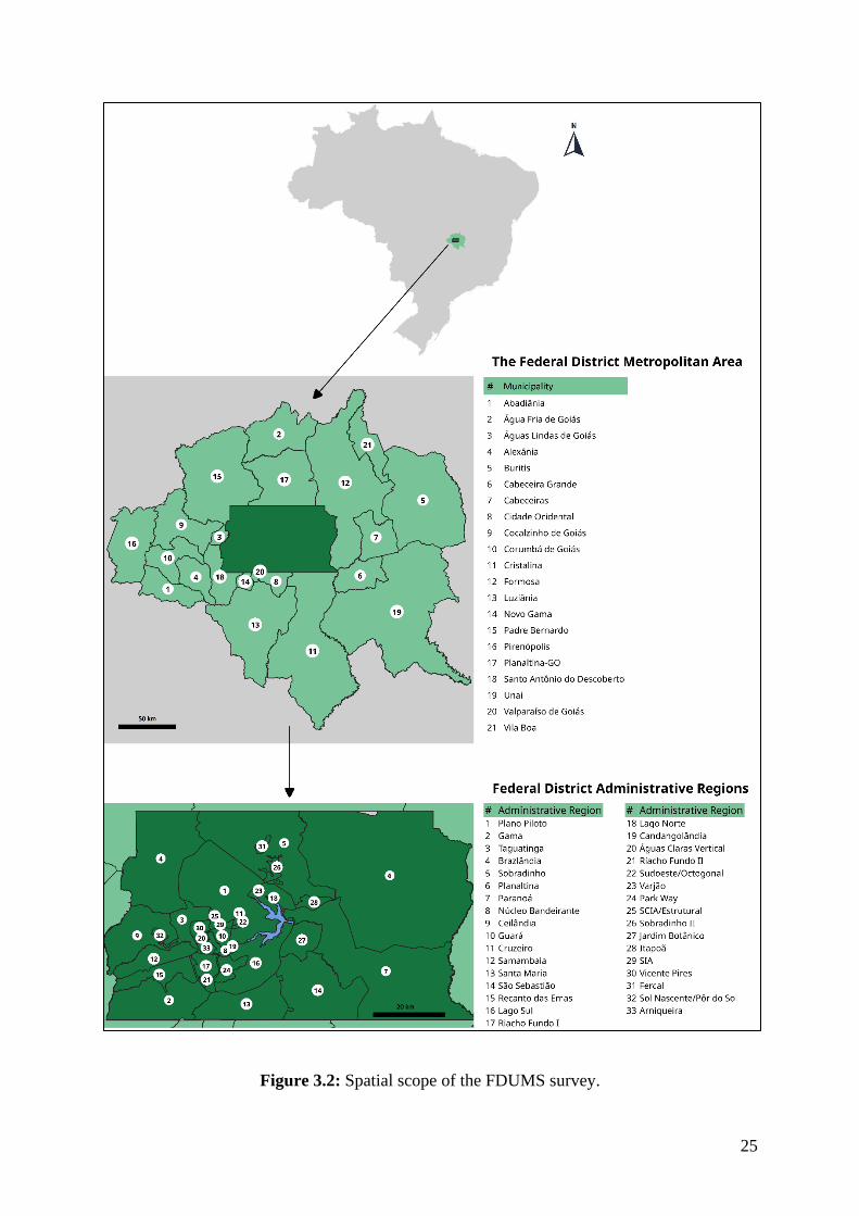
The spatial scope of the survey is presented in Figure 3.2.

25

Figure 3.2: Spatial scope of the FDUMS survey.

26

Results of the FDUMS were made available as four separate tables, characterized as follows:

• Table Domicilio (Household): an identification number was assigned to each household

that was part of the survey, and that is the primary key of this dataset. This table includes

data such as the administrative area where the household is located, the number of

people that lives within the household, number of rooms of the household (number of

bedrooms, bathrooms), number of vehicles owned (cars, bicycles, motorcycles), total

income of the family, and other socioeconomic information.

• Table Morador (Person): this table is composed by information about the residents of

each household that was part of the survey, and these individuals were identified by a

number, which is the primary key of the dataset. Data such as age, gender, education

achieved, employment and driver’s license ownership for each person are available.

Obviously, there is also the identification number of the household the person is part of,

which allows cross-referencing with information of the dataset described previously

(table Domicilio).

• Table Viagem (Trip): this table consolidates information about the trips that survey’s

respondents perform on a typical day. It is the travel diary that was mentioned along this

document. The primary key of this dataset is the identification number of the trip, but

the identification number of the person which performed the trip is also available. Trips

are defined by their origin and destination locations (on the administrative regions level

and on microzoning level as well), transportation mode used during the trip, trip purpose

(activity that will be performed on the destination), start and end times, and other details.

• Table Etapa (Stage): this table regards details about each step of a trip. For instance,

there are trips performed between locations A and B, but in the meantime the person

needs to take different transportation modes (maybe a bus and then a train). The purpose

of this table is to present these details of the trips’ steps. The primary key of this dataset

is the identification number of the steps, but the number of the trip they are related with

is also available. This table will not be used in the current study, because information

available on table Viagem (Trip) is sufficient for the purpose of the model.

27

All tables that compose the FDUMS survey results were translated into English and they were

made publicly available in the Kaggle online community of data science and machine learning

practitioners (MIRANDA, 2020).

3.3.2 Obtaining and organizing the socio-demography (soc) dataset

The process of obtaining the soc dataset was pretty straightforward, as most of the required

variables had been collected directly in the FDUMS. For instance, the features gender and

driver’s license, that are described by Drchal et al. (2019) as part of the soc dataset, were

obtained directly from the FDUMS dataset, as binary variables with the possible answers

“male” or “female” and “yes” or “no”, respectively. On the organized dataset that was used in

the current study, these variables were called gender and has_driver_license.

Another required variable was age, whose type was not defined on the article that originated

the model. In the FDUMS dataset, age information for each agent was presented as a categorical

variable, with thirteen possible age ranges. On the organized dataset, this feature was called

age_group. The variable education level was also a categorical variable in the FDUMS dataset,

with eleven possible answers. This is slightly different from the original model described by

Drchal et al. (2019), where there were three possible answers for the education level variable:

low, mid or high.

The household size feature referred to the number of people that lived in the individual’s

household. This information was obtained with a cross-referencing process between the

FDUMS Household and Person tables, as the number of inhabitants of each household was

presented in the Household table and this information had to be disaggregated for each

individual. On the organized dataset, this feature was identified as the household_size integer-

typed variable. The same process was required to obtain the car available feature, which

indicated whether there was a car in the individual’s home or not. On the organized dataset, this

feature was identified as the is_car_availabe binary (“yes” or “no”) variable. The student

feature, which described whether the person was a student or not, was obtained with a similar

process, but by using cross-referencing between the FDUMS Trip and Person tables. If the

person had any activity of the type study in his/her schedule, he/she was considered to be a

student. On the organized dataset, this feature was identified as the is_student binary (“yes” or

“no”) variable.

28

The variable public transportation pass, which indicated whether the person owned a public

transportation card and was described by Drchal et al. (2019) as part of the soc dataset, was not

available on the FDUMS datasets, thus it was not considered in this study. Finally, Table 3.1

presents the features that compound the organized soc dataset developed for the model of the

current research.

Table 3.1: Features of the organized soc dataset.

Column name on

the organized

dataset

Value type on

the organized

dataset

Description Column name on the

FDUMS dataset

Equivalent

feature on

the original

DDAS

model

person_id Integer Identification code for

each individual

TABLE Person:

person_id -

household_id Integer

Identification code for

the household to which

the individual belongs

TABLE Person:

household_id -

household_size Integer

Number of people that

live in the individual’s

household

TABLE Household:

people_in_the_household

TABLE soc:

household

size

age_group Categorical

(13 options)

Age range of the

individual TABLE Person: age

TABLE soc:

age

gender Binary (male or

female) Gender of the individual TABLE Person: gender

TABLE soc:

gender

is_car_availabe Binary

(yes or no)

Whether there is a car

available in the

individual’s household

IF(TABLE Household:

vehicles >= 1)

TABLE soc:

car available

is_student Binary

(yes or no)

Whether the individual

is a student

IF(TABLE Trip HAS

“Study”)

TABLE soc:

student

education_level

Categorical

(11 options)

Education level

achieved by the

individual

TABLE Person:

education_level

TABLE soc:

education

achieved

(3 options)

has_driver_license Binary

(yes or no)

Whether the person has

a driver license

TABLE Person:

has_driver_license

TABLE soc:

driver’s

license

Up to this point of the data organization process, the input dataset is composed by 61,358

individuals, which is the number of respondents to the FDUMS. However, some data selection

is required in order to keep data consistency before running the model. First, it was conducted

a removal from the dataset of rows that represented individuals for which there was no reference

on the Trip table, which means that no activity schedule was collected for that person during

the survey (17,257 instances, or 28.1% of the original dataset). Then, rows with missing values

29

were deleted (when the interviewee decided not to answer the question). There were found 239

rows with missing values for at least one of the features (0.54% of the remaining records).

In sequence, individuals that are 14 years old or younger were removed from the dataset,

because the intention is to analyze transportation choice and behavior, and it is clear that

children often follow their parents and do not have this decision capacity. This group

represented 7,280 individuals (16.6% of the remaining dataset). Finally, individuals who had

incomplete schedules (diaries that did not start and finish at home) were deleted. After all this

selection process, the soc dataset organized for being an input to the model had 34,340 rows

(individuals’ records).

3.3.3 Obtaining and organizing the reach dataset

As it was described in section 3.1.2, the reach dataset that is required as input by the DDAS

model includes features that represent an estimation of the trip duration between the person’s

home and the place where he/she performs their main activity (work or school). This

information was not directly available from the FDUMS data, so a method was developed to

obtain it. Considering that the reach descriptor was calculated on the administrative region

level, it was developed a matrix of trip durations between pairs of origin-destination

administrative areas, that is identified as a trip duration matrix. An example of this kind of

matrix is presented in Figure 3.3.

Figure 3.3: Example of a trip duration matrix.

30

In Figure 3.3, values dij represent the average trip duration between regions i and j, on a regular

weekday, at 8 AM, using a certain type of transportation mode. The idea is that if there is a trip

duration matrix for all administrative areas in Federal District and the municipalities that

compose the Brasilia’s Metropolitan Area, queries may be performed in this matrix for the reach

descriptor of each individual in the dataset, considering the place he/she lives is known and so

is the place where he/she performs his/her main activity (work or study).

In order to create the trip duration matrix for the Federal District administrative areas, the

following input data was used:

• An ESRI Shapefile set of documents, in which the polygon layer is formed by features

representing the administrative areas, whose names are presented in a field. For the model,

the Shapefile was available as one of the products of the Federal District Rail Transit

Development Plan, together with the FDUMS. The vector was composed by the 31

administrative areas (or neighborhoods) of the Federal District and the 21 municipalities

that form the Brasilia Metropolitan Area.

• Lists containing the name of the administrative areas or municipalities that must be

considered as origins and destinations on the trip duration matrix. For the purpose of this

research, these lists were obtained from the FDUMS datasets and registered them on the

CSV (comma-separated values) format.

The algorithm to create the trip duration matrix was developed in Python programming

language. First, a randomPoint function was defined for converting the Shapefile polygon into

points and then returned the coordinates for one of these points. Then, it was defined a

commuteTime function that returned the trip duration between two points, given a day and a

transportation mode, using the Google Maps API. Finally, the randomPoint function was

applied to select origin and destination points for each pair of administrative regions and use

them as input to the commuteTime function. The commuteTime was calculated for three pairs

of points, for each pair of administrative regions, and filled in the trip duration matrix instance

with the average of these values.

Trip duration matrices were developed for the transportation modes: car, public transportation,

walking, and bike. To be consistent with the model developed by Drchal et al., (2019), if there

31

was no connection from the person’s home to his/her main activity location given a certain

mode (for instance, there is no public transportation accessibility for these regions), a value of

-1 was assigned for the reach feature. Detailed description of the procedure for creating trip

duration matrices and the results obtained for the described dataset may be found on

Appendix C.

An issue that was verified during the process of creating the reach dataset was that some of the

trip records for the individuals included a destination named “External”, that was not described

on the dataset documentation. Since the frequency of these occurrences was low (119

individuals, or 0.33% of the total records of the database that was developed in section 3.3.2),

it was decided to simply remove these rows from the dataset.

3.3.4 Obtaining and organizing travel information

To conclude the organization of the input dataset, it was required to include information about

the trips performed by the agents. Three columns are now appended to the organized dataset:

activity_origin (meaning current activity type), activity_destination (next activity type) and

mode_type (referring to the travel mode choice). These features are available on the FDUMS

table Trip (Viagem).

In the framework proposed by Drchal et al. (2019), possible activity types are: sleep, work,

school, leisure and shop. Activity type sleep means the individual is at home. In the FDUMS

dataset, however, activity types are organized into different categories. Thus, a new activity

type other was created, although it was not part of the original set of categories, in order to

incorporate some of the FDUMS types, which included 15.4% of all trips recorded. Table 3.2

displays the correspondence made between these different groups.

The same issue was verified for the travel mode choice variable, which is called

modoagregado2 on the FDUMS dataset. Although the original method presented by Drchal et

al. (2019) only included the modes car, pt (for public transportation), walk and bike, a variable

other_mode was created to aggregate the options TI_publico (public individual transportation

– such as taxis), Outros (translated as other) and Combinado (translated as multiple modes).

They summed up 1.18% of travel mode choice frequency. Table 3.3 displays the

correspondence made between the FDUMS and the final organized dataset created as input for

the model.

32

Table 3.2: Correspondence between activity types on the organized dataset and on the

FDUMS dataset, and respective frequencies

Activity

type on the

organized

dataset

Activity type on the FDUMS dataset

Frequency of

activity type

for destinations

Relative

frequency (%)

of activity type

for destinations

leisure Lazer (leisure) 2,331 2.1%

school

Local de estudo regular

(main study place) 13,481 11.9%

Local de estudo secundário

(secondary study place) 810 0.71%

shop Compras (shopping) 3868 3.4%

Refeição (eating out) 808 0.71%

sleep Residência (home) 51,785 45.7%

work

Local de Trabalho Principal

(main workplace) 21,052 18.6%

Local de Trabalho Secundário

(secondary workplace) 573 0.51%

Negócios/A Serviço (business) 1,177 1.04%

other

Levar ou Acompanhar outra Pessoa

(accompany someone) 7,538 6.7%

Assuntos Pessoais (personal business) 6,322 5.6%

Saúde (health) 2,606 2.3%

Outros (other) 1,042 0.92%

Table 3.3: Correspondence between mode types on the organized dataset and on the FDUMS

dataset, and respective frequencies

Mode type

on the

organized

dataset

Mode type on the FDUMS dataset Frequency of

mode type for

Relative

frequency (%)

of mode type

bike TA_Bicicleta

(active transportation: cycling) 1,941 1.71%

car TI_Privado

(private individual transportation) 53,777 47.4%

pt

TC_Público

(public collective transportation) 24,616 21.7%

TC_Privado (private collective

transporation – chartered buses) 3,393 3.0%

walk TA_aPe

(active transporation: walking) 28,338 25,0%

other_mode

TI_Público (individual public

transporation – taxis) 455 0.40%

Combinado (multiple modes) 598 0.53%

Outros (other) 280 0.25%

33

Finally, the count set of variables, as described in 3.1.2, was included in the form of six columns,

each one representing an activity type (sleep, work, school, leisure, shop, and other_mode). For

each row of the table (leg of a trip), a number representing the count of activity types performed

up to that point of the trip was included in each of these columns.

3.3.5 Converting feature types

As described in section 2.2.1.2, in this study the Scikit-learn Python library is used to implement

the decision-tree classifier algorithm. However, the current version of this model does not

support categorical variables (SCIKIT-LEARN USER GUIDE, 2020a). For this reason, the

encoding on the categorical features of the dataset was required.

For the binary variables (gender, is_car_avaiable, is_student, has_driver_license) this process

was simple, as possible values were converted into “0” or “1”. The only categorical feature left

was activity_origin.

The Scikit-learn Python library provides two native options for performing encoding on

categorical features: the ordinal encoder and the one-hot encoder (SCIKIT-LEARN USER

GUIDE, 2020b). The ordinal encoder, also known as “label encoder”, transforms each possible

answer into an integer number. For instance, for the activity_origin feature, its possible values

“leisure”, “school”, “shop”, “sleep”, “work” and “other” could be replaced by the numbers “1”,

“2”, “3”, “4”, “5” and “6”, respectively. However, this process makes it seem like there is some

kind of ordering in the possible activity types, which is not true. That is why label encoding is

only recommended for features which values have an intrinsic order associated (GRADY &

MEDOFF, 1988).

So, it was decided to perform one-hot encoding on the activity_origin feature. In one-hot

encoding, each possible value of the categorical feature is turned into a new column on the

dataset, or into a new feature. For each instance (row) of the dataset, the column associated with

the actual value of the feature receives the number 1 and the others receive 0. This process is

demonstrated in Figure 3.4.

The detailed procedure for data preparation is presented in the first part of Appendix D.

34

Figure 3.4: Example of the one-hot encoding (OHE) process.

3.3.6 Profiling the organized dataset

In the organized dataset, after concluding the cleansing process, the proportion of female

individuals was slightly higher than male (51.5% and 48.5%, respectively). These values are

consistent with the proportions observed in the Brazilian Census of 2010 for the Federal District

region, with 52% of the population being female and 48% male (IBGE, [s.d.]). Figure 3.5

displays the gender profiling of the original and clean datasets.

Figure 3.5: Profile of the “gender” feature on both the original and the clean datasets.

The majority of individuals that composed the organized dataset ranged in age from 30 to 49

years old (39.7% of the instances), as can be observed in Figure 3.6. In section 3.3.2, it was

described that individuals younger than 15 years old were removed from the working dataset

due to their inability for providing meaningful insights regarding decision making processes.

35

Figure 3.6: Profile of the “age” feature on both the original and the clean datasets.

Figure 3.7 indicates that more than 38% of the individuals that composed the organized dataset

had at least an undergraduate degree. The removal of individuals younger than 15 years old

from the working dataset contributed to the increase on the average education level in the

organized set of data.

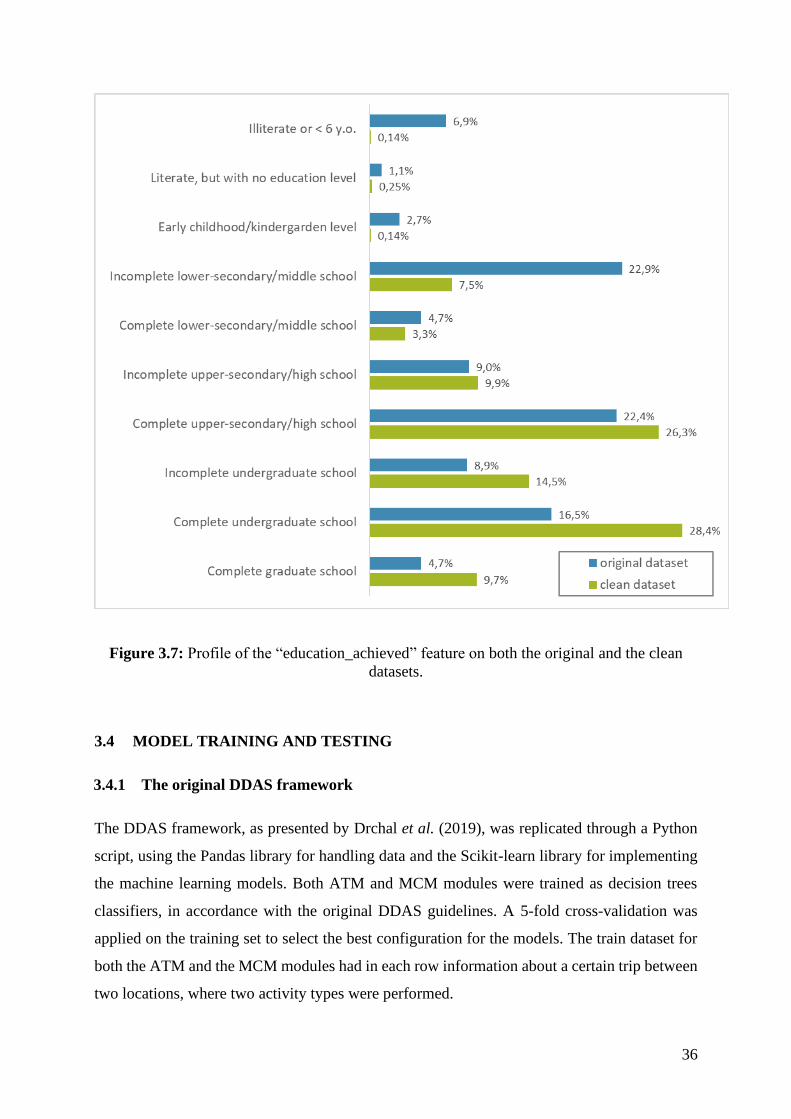
36

Figure 3.7: Profile of the “education_achieved” feature on both the original and the clean

datasets.

3.4 MODEL TRAINING AND TESTING

3.4.1 The original DDAS framework

The DDAS framework, as presented by Drchal et al. (2019), was replicated through a Python

script, using the Pandas library for handling data and the Scikit-learn library for implementing

the machine learning models. Both ATM and MCM modules were trained as decision trees

classifiers, in accordance with the original DDAS guidelines. A 5-fold cross-validation was

applied on the training set to select the best configuration for the models. The train dataset for

both the ATM and the MCM modules had in each row information about a certain trip between

two locations, where two activity types were performed.

37

Therefore, in each row, soc and reach information of the agent that was performing the trip

were included, even if this agent performed a number of trips, what caused these personal

features to be repeated along many rows. The test dataset, on the other hand, included only soc

and reach features for the agents. The other features were created along with the algorithm, as

the schedules were developed by the model (e.g.: the activity type counters, mode counters).

The complete scripts developed for conducting this research were made publicly available in

the Kaggle online community of data science and machine learning practitioners and they are

also presented on Appendix D.

The output of the test algorithm is a table similar to the one used for training the models, with

one trip represented in each row (pairs of origins-destinations and activity types). By grouping

the rows of trips performed by the same agent, it is possible to describe the predicted daily

activity schedule for that agent, and compare it with the actual schedule from the test dataset,

using the validation frameworks described in section 3.2.

Regarding the validation framework (VALFRAM), the chi-square values were computed by

using Yates’s correction for continuity (YATES, 1934). This procedure was not explicitly

described on the original DDAS paper, but it was necessary for dealing with occasional zero

occurrences on the contingency tables. Based on the formula for Pearson’s chi-square test, a

unit value was subtracted from the difference between each observed and expected values, as

demonstrated in Equation 3.2, where 𝑂𝑖 is an observed frequency, 𝐸𝑖 is an expected frequency

and 𝑁 is the number of distinct events.

𝑋𝑌𝑎𝑡𝑒𝑠2 = ∑

(|𝑂𝑖−𝐸𝑖|−0.5)2

𝐸𝑖,𝑁

𝑖=1 Equation 3.2.

It is important to note that on the original DDAS framework, one of the outputs of the MCM

module was the trip duration, as it was a function of the chosen mode. However, it was also a

function of the activity locations predicted by the AAM module, which was not implemented

in the current study.

Another difference between the original DDAS framework and the model that was implemented

in this study regards the set of hard-coded rules that existed in the model proposed by Drchal et

al. (2019). The authors emphasized that the intention was to eliminate as many expert rules as

38

possible, but due to the limited size of their sample (2600 agents from 1000 households) and,

therefore, their training set, they had to enforce some constraints. An example was the rule that

for MCM module, only modes available to the person were allowed (e.g.: the car mode was

only allowed for agents who actually had a car). This type of constraints was not implemented

in the current study because the valid sample size used was larger (more than 34,000 agents,

after data cleaning), so it was admitted that the model would be able to learn the rules by itself.

39

4 RESULTS AND ANALYSIS

In this chapter, three sets of results are presented. First, a replication of the DDAS framework

is conducted, by following the same procedures proposed by Drchal et al. (2019) and described

in Chapter 3. This DDAS replication is identified as Model 1. Based on the results obtained

from Model 1, improvements on the Decision Tree Classifier architectures for the ATM and

MCM modules are proposed and tested on a second model, which is identified as Model 2.

Lastly, a third model, identified as Model 3, is tested by changing the core Decision Tree

Classifier by an ensemble model, the Random Forest classifier. At the end of this chapter, a

comparison between the three sets of results is presented. As this is the first replication of the

DDAS method, which is unique compared to other modeling frameworks, emphasis was placed

on comparing the results obtained in this implementation with the originals obtained by Drchal

et al. (2019). Therefore, comparison of results with others in existing literature regarding

activity-based modeling was not the focus of this chapter.

4.1 MODEL 1: THE ORIGINAL DDAS FRAMEWORK

4.1.1 Training results for Model 1

In the original DDAS framework, the optimal depths for the ATM and MCM decision tree

models are selected by maximizing the F1-score (specifically the micro-averaged F1-score). In

the current implementation of DDAS, the same procedure was followed. Figure 4.1 presents

the results obtained for cross-validation training on ATM module, and Figure 4.2 presents the

same information for the MCM module. For each depth of the models, a 5-fold cross-validation

was conducted. The orange line on these figures indicate the mean F1-score obtained on the

training subset for the cross-validation conducted. The blue line, on its turn, indicates the mean

F1-score obtained for the cross-validation test subset, while the blue area on the figures

represent the range of ± 2 standard deviations from the mean F1-score on cross-validation.

Table 4.1 displays the consolidated results for each module, comparing the optimal values

found by the current DDAS implementation with the original DDAS results presented by

Drchal et al. (2019). The 5-fold cross-validation with 50 depths on the ATM module took 4

minutes and 14 seconds to run on the cloud computational environment Kaggle, and MCM

module cross-validation took 5 minutes and 3 seconds to run the same cross-validation on the

same computational environment.

40

Figure 4.1: Selection of ATM tree depth via cross-validation for Model 1,

F1-score vs. tree depth.

Figure 4.2: Selection of MCM tree depth via cross-validation for Model 1,

F1-score vs. tree depth.

Table 4.1: F1-scores for training the ATM and MCM modules of Model 1, compared to the

results presented by Drchal et al. (2019), which is DDAS original implementation.

Model

ATM MCM

Max. mean

F1-score

Optimal

tree depth

Max. mean

F1-score

Optimal

tree depth

Drchal et al. (2019) 0.87 6 0.83 8

Model 1 0.637 6 0.821 10

41

It can be observed from Figures 4.1 and 4.2 that the ATM module F1-scores in cross-validation

had a higher variance than the scores obtained for the MCM module, and this variance increases

as the tree depth increases.

The results in Table 4.1 indicate that optimal tree depths found in the current implementation

of DDAS and in its original implementation were similar. However, the values for the

maximum F1-scores were only similar for the MCM module, while in the ATM module the F1-

score obtained for the current implementation was 26% lower than in the original study. It is

difficult to compare this result with other studies in literature because the prediction approach

of DDAS is innovative. As described in Chapter Erro! Fonte de referência não encontrada.,

usually, activity-based models are designed to directly predict the full pattern of activity each

person should perform. For instance, given a list of possible activity patterns, extracted from

the most common patterns observed on the training set, the model selects the one the activity

chain that will be performed by each person on their schedules (TACO, 2003; M. YANG et al.,

2014; ZHAO & SHAO, 2010). On the other hand, DDAS proposes sequential prediction of

each trip, so the models are trained by predicting one trip at a time, having a prediction accuracy

for individual trips. Therefore, comparison with existing studies is impracticable.

Using the optimal tree depths that were obtained from cross-validation, confusion matrices for

both the ATM and the MCM modules were developed by performing an 80-20 training-test

subset split on the training set. This analysis was not presented on the original DDAS paper,

but it may provide useful insights on the model performance. Figure 4.3 presents the confusion

matrix for the ATM module and Table 4.2 displays a report that includes various score metrics

for each class (possible activity types).

By observing Figure 4.3 and Table 4.2, a result that draws attention is that no activity of types

leisure, shop or sleep were predicted, although in the training subset for cross-validation there

were 278, 648 and 1407 occurrences of that activity types, respectively. For most of the cases

in which the true value was leisure or shop, the trained ATM module predicted the class to be

work, other or none (ending the agent’s schedule). These types are the most common true results

on the cross-validation set. Virtually for all cases in which the true value was sleep, the class

was predicted as none (ending the agent’s schedule). These results contributed to the low overall

F1-score of the model.

42

Figure 4.3: Confusion matrix for a cross-validation set of the ATM module, adopting the

optimal tree depth that was previously found (depth = 6).

Table 4.2: Score metrics for a cross-validation set of the ATM module, adopting the optimal

tree depth that was previously found (depth = 6).

Class Precision Recall F1-score True

counts

leisure 0 0 0 278

none 0.680 0.981 0.803 5559

other 0.504 0.266 0.348 2493

school 0.743 0.701 0.722 1095

shop 0 0 0 648

sleep 0 0 0 1407

work 0.585 0.784 0.670 3305

full model – micro averaged - - 0.641 -

full model – macro averaged 0.359 0.390 0.363 -

full model – weighted averaged 0.527 0.641 0.564 -

Figure 4.4 presents the confusion matrix that was obtained for the MCM module, by following

the same procedure that was described for the ATM module. Table 4.3 displays the score

metrics with respect to this confusion matrix.

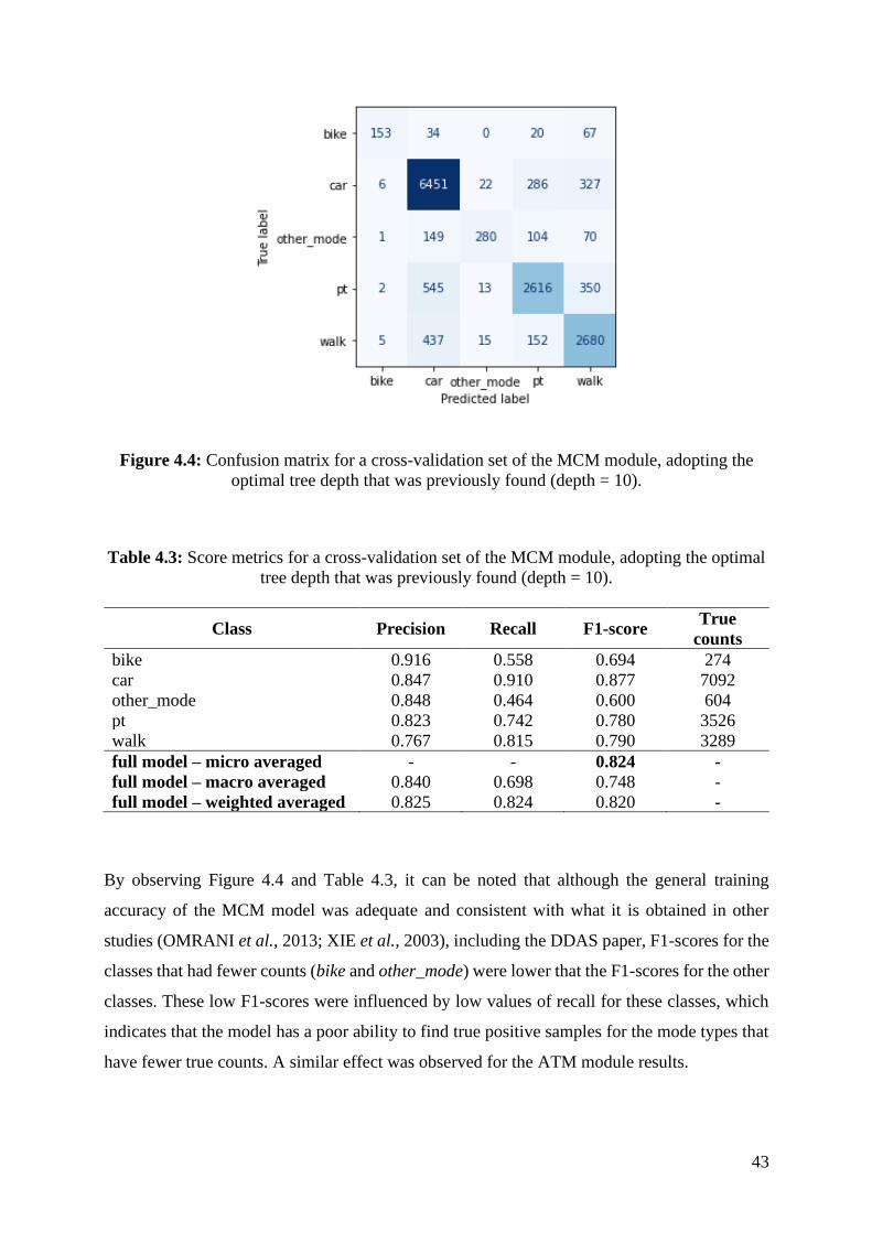
43

Figure 4.4: Confusion matrix for a cross-validation set of the MCM module, adopting the

optimal tree depth that was previously found (depth = 10).

Table 4.3: Score metrics for a cross-validation set of the MCM module, adopting the optimal

tree depth that was previously found (depth = 10).

Class Precision Recall F1-score True

counts

bike 0.916 0.558 0.694 274

car 0.847 0.910 0.877 7092

other_mode 0.848 0.464 0.600 604

pt 0.823 0.742 0.780 3526

walk 0.767 0.815 0.790 3289

full model – micro averaged - - 0.824 -

full model – macro averaged 0.840 0.698 0.748 -

full model – weighted averaged 0.825 0.824 0.820 -

By observing Figure 4.4 and Table 4.3, it can be noted that although the general training

accuracy of the MCM model was adequate and consistent with what it is obtained in other

studies (OMRANI et al., 2013; XIE et al., 2003), including the DDAS paper, F1-scores for the

classes that had fewer counts (bike and other_mode) were lower that the F1-scores for the other

classes. These low F1-scores were influenced by low values of recall for these classes, which

indicates that the model has a poor ability to find true positive samples for the mode types that

have fewer true counts. A similar effect was observed for the ATM module results.

44

As it is displayed in the confusion matrix, other_type occurrences are usually mispredicted as

car or pt mode types, which are the classes that have most counts on the cross-validation subset.

The bike mode type also has few true counts on the cross-validation subset. However,

something interesting is observed in the confusion matrix for the bike class: true instances are

usually confused with the walk mode instead of being confused with more common classes

such as car or pt. This indicates that there may be nodes on the decision tree that successfully

discriminates active transportation modes from motorized transportation modes.

Both ATM and MCM were trained on the full training set using the configuration that was

obtained from cross-validation. This training took 1.1 second to run on the cloud computational

environment Kaggle. Test results are presented on the next subsections.

4.1.2 Test results for Model 1: general

After the training of the ATM and MCM modules, the models were run as part of the DDAS

framework implementation that was described in Chapter 3 of this document, using the test

dataset (6868 agents). This implementation took 3 minutes and 27 seconds to run on the on the

cloud computational environment Kaggle, considering that the models were already trained.

4.1.3 Test results for Model 1: ATM module

4.1.3.1 Expected and observed distribution of trips

The first analysis that is presented on the results regards the expected (from the test set) and

observed (model predictions) distribution of trips. This analysis was not presented in the

original DDAS paper (DRCHAL et al., 2019), but it is being included in the current study due

to its importance for evaluating model performance. Figure 4.5 displays these results.

It is possible to note that the model did not predict any activities of the type leisure or sleep and

had almost no prediction of activities of the type shop. On the other hand, the model predicted

more activities of types none and work that what was expected. These results were anticipated

on the analysis conducted during the training phase, in which it was observed that the model

often misclassified less frequent activities, such as shop and leisure as being more common

types, such as work.

45

The misclassification of activities with the true label sleep as being none indicate that the model

is predicting shorter chains than what is expected. This hypothesis is verified on the next

subsection.

Figure 4.5: Comparison between the expected and observed proportions of activity types on

the agent’s schedules, for Model 1.

4.1.3.2 Expected and observed frequency of activity chains

Although it was not part of the original DDAS validation framework, as presented by

Drchal et al. (2019), in the current study a comparison between expected and observed

frequency of activity chains was conducted, in order to evaluate model performance. Results

are presented in Table 4.4.

Table 4.4: Expected and observed frequency of activity chains for Model 1.

Type of activity

chain

Frequency on the

test dataset

(expected values)

Type of activity chain

Frequency on the

results dataset

(observed values)

HWH 2467 (36%) HWH 4495 (65%)

HOH 915 (13%) HOH 1331 (19%)

HSH 789 (11%) HSH 1040 (15%)

HBH 347 (5%) HBH 1 (<1%)

Other patterns

(449 instances) 2350 (34%) HOOOOOOOOOOOOH 1 (<1%)

TOTAL 6868 schedules TOTAL 6868 schedules

46

It is possible to observe from Table 4.4 that, as anticipated on the analysis of the previous

subsection of this document, predicted chains are indeed shorter than it was expected. It appears

that the model simplifies the chain performed by a person, predicting practically only 2-trips

schedules, while the actual values contained 454 possible activity chain patterns.

Another interesting result that was obtained was the one awfully long and repetitive chain that

were predicted. Apparently, this chain would be infinite if there was not a hard-coded rule that

stopped all chains that had more than 14 trips. It is a signal that the count features of the model,

which represent how many trips of each type the agent has performed up to that point of the

schedule, may not be taking into consideration by the model. In order to evaluate that, the next

section presents the analysis of importance of the features for the model.

4.1.3.3 Analysis of importance of the features

On the Scikit-learn library for Python, the function permutation_importance is computed as the

decrease in a model score when a single feature value is randomly shuffled. Table 4.5 presents

the average values for permutation_importance obtained for 5 repeats of shuffling the ATM

module training sets in Model 1.

It is clear from Table 4.5 that features related to activity counts have low impact on model

performance. This could explain the prediction of that long and repetitive chain presented in

the previous subsection. Another interesting result that can be obtained from the analysis of

Table 4.5 is that the feature that indicates whether the individual is currently on a work activity

is not relevant at all for predicting him/her next activity. On the other hand, the feature that

indicates whether the person is at home has the highest importance on the prediction of the next

activity, by a large difference from the other features. This may indicate that the decision tree

is working with the following basic premises: every time the person is at home, the model

predicts the next activity as being any other kind (based on the most common activity types);

every time the person is on an activity type that is not home, the model finishes the schedule.

47

Table 4.5: Permutation importance for features of the ATM module in Model 1.

Feature Importance

on Model 1

is_origin_sleep 0.298876

is_student 0.070084

age_group 0.020070

is_female 0.010928

reach_bike 0.010492

education_level 0.005790

reach_car 0.000942

has_driver_license 0.000317

people_in_household 0.000084

is_origin_other 0.000068

reach_transit 0.000041

count_work 0.000022

is_origin_shop 0.000000

is_origin_school 0.000000

is_origin_leisure 0.000000

count_leisure 0.000000

count_sleep 0.000000

count_shop 0.000000

count_school 0.000000

count_other 0.000000

reach_walk 0.000000

is_car_available 0.000000

is_origin_work 0.000000

4.1.3.4 Activity counts validation

The last analysis to be performed on the ATM results regards the VALFRAM validation for

activity counts. Comparison between expected and observed values for each class (activity

type), including the chi-square measure, as described in Chapter 3, are presented in Figure 4.6.

The aim of the Pearson’s chi-square (Χ2) statistical test is to verify goodness of fit, or whether

an observed frequency distribution is similar to a theoretical distribution. As described in

Chapter 3, the objective of the current analysis is to determine if the real values (from the

FDUMS dataset) and the predicted distributions using the ATM module on Model 1 are

statistically different.

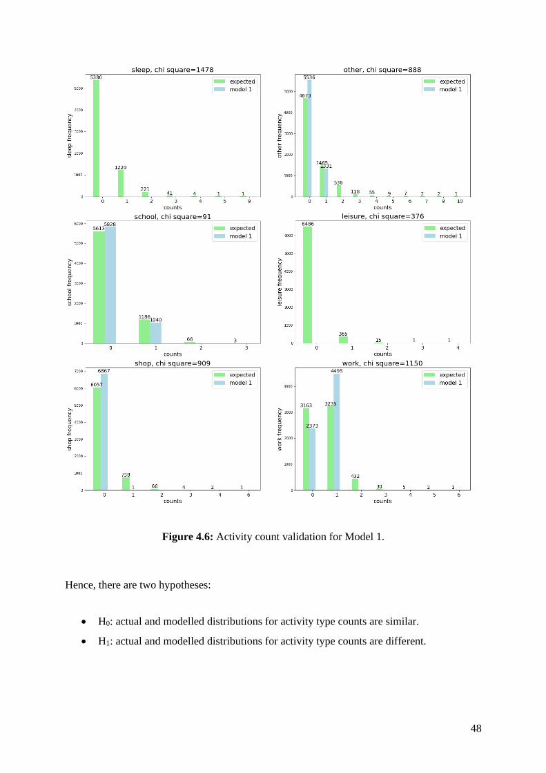
48

Figure 4.6: Activity count validation for Model 1.

Hence, there are two hypotheses:

• H0: actual and modelled distributions for activity type counts are similar.

• H1: actual and modelled distributions for activity type counts are different.

49

Based on the Χ2 value, it is possible to calculate what is called p-value, which is the risk of

incorrectly rejecting the H0 hypothesis. The results obtained for the Model 1, which are

presented in Figure 4.5 favored the rejection of H0, as the Χ2 values were extremely high, and

all p-values were equal to zero.

As discussed on the previous topics, there are a lot of factors that lead to the bad performance

of the model, many of them related to the unbalance of class distribution on the training set.

4.1.4 Test results for Model 1: MCM module

Again, VALFRAM indicates the chi-square (Χ2) statistical test for verifying goodness of fit, or

if the real values (from the FDUMS dataset) and the predicted distributions using the MCM

module on Model 1 are statistically different. Chapter 3 describes the adjustment that was made

on the chi-square computation to adequately compute mode count distributions for each mode.

Results are presented in Figure 4.7.

Hypothesis testing is similar to the one performed for ATM validation:

• H0: actual and modelled distributions for mode counts given an activity are similar.

• H1: actual and modelled distributions for mode counts given an activity are different.

It is interesting to note that although MCM module performed well on training, with a good

overall score of prediction, validation results report that the model did not perform well on the

global DDAS framework. The results obtained for the Model 1, which are presented in Figure

4.7 favored the rejection of H0, as the Χ2 values were extremely high, and all p-values were

equal to zero.

This bad performance of the model on test may be due to the design of the validation

framework. Since mode counts are computed for groups of given activity types, errors on the

ATM module may propagate to the MCM module. An example of that is mode count for

activity types leisure, shop and sleep. The Χ2 values for each activity type are calculated based

on the proportions expected and observed. However, since no leisure or sleep activities were

predicted, Χ2 for mode count validations on these classes were equal to zero, given a false idea

that expected and observed distributions were similar. The same effect was observed for the

activity of type shop, which was only predicted once.

50

Figure 4.7: Travel mode choice validation for Model 1.

51

Thus, an improvement on the ATM module might improve the results of the MCM module.

Moreover, improvement could be made also on the travel mode choice validation technique

that is proposed in the VALFRAM framework for activity-based models.

4.1.5 Partial conclusions after implementing Model 1

In this subsection, Model 1 was developed as being a simple reproduction of the ATM and

MCM modules from the DDAS framework. Results indicated that the ATM module needs

improvement because its results are not consistent, nor during training or during test. On the

other hand, by analyzing MCM performance on training, it could be said that the model is

adequate as it is. Improvement on the ATM module might lead to better validation results on

the MCM module.

The categorical features being targeted for prediction on this study (activity type and

transportation mode) are highly imbalanced, with some classes being way more frequent than

others. As presented in Chapter Erro! Fonte de referência não encontrada., the micro-

averaged F1-score may not be the ideal score function for evaluating prediction models when

classes are imbalanced. Therefore, selection of tree depth for the ATM and MCM modules

should be done with another score function, such as balanced accuracy, for instance. It could

lead to tree configurations that produce more plausible activity diaries.

Another possibility for improving accuracy of the model with imbalanced training sets would

be to use methods such as Synthetic Minority Over-Sampling Technique (SMOTE), to

synthetically balance the classes.

4.2 MODEL 2: IMPROVING THE DECISION TREE CLASSIFIER

4.2.1 Changing the score function for Model 1

Based on the results obtained on the previous subsection, all procedures that were conducted

for developing Model 1 were run again, but this time changing the score function that was

previously the micro-averaged f1-score to the balanced-accuracy, which is more convenient

for imbalanced datasets. Maximum tree depth for both ATM and MCM were selected based on

optimal values for the score function.

52

Figure 4.8 presents the results obtained for cross-validation training on ATM module, and

Figure 4.9 presents the same information for the MCM module. Table 4.6 displays the optimal

depths found by using the balanced accuracy score function.

Figure 4.8: Selection of ATM tree depth via cross-validation, for Model 1,

balanced accuracy vs. tree depth.

Figure 4.9: Selection of MCM tree depth via cross-validation, for Model 1,

balanced accuracy vs. tree depth.

53

Table 4.6: Balanced accuracy scores for training the ATM and MCM modules of Model 1.

Model

ATM MCM

Max. mean

balanced

accuracy

Optimal

tree depth

Max. mean

balanced

accuracy

Optimal

tree depth

Model 1 0.394 10 0.684 10

An optimal tree depth of 10 was found for the ATM module by using the balanced accuracy

score function on cross-validation. It is not far from the optimal depth of 6 found previously by

using the f1-score. Actually, from Figure 4.8, it can be observed that the average balanced

accuracy for depth 6 is virtually the same as for depth 10, which means that only changing the

score function for cross validation did not bring improvements on the model, as the optimal

depth remained the same. The same occurred for the MCM module.

4.2.2 Training Model 2 using the SMOTE technique

Based on the results obtained from Model 1, which indicated that the dataset that is being

studied has highly imbalanced target features, the SMOTE technique was tested on training the

ATM and MCM modules in order to try achieving better balanced accuracy scores. This

approach is identified on this document as Model 2.

Figure 4.10 presents the results obtained for cross-validation training using SMOTE on ATM

module, and Figure 4.11 presents the same information for the MCM module. Table 4.7

displays the optimal depths found by using the balanced accuracy score function.

It can be concluded from the results on Table 4.7 that the use of the SMOTE technique was

able to improve the maximum balanced accuracy on training of both the ATM and MCM

modules.

Then, both ATM and MCM were trained on the full training set using the configuration that

was obtained from cross-validation, including the SMOTE technique. This training took

9.6 seconds to run on the on the cloud computational environment Kaggle. Test results are

presented on the next subsections.

54

Figure 4.10: Selection of ATM tree depth via cross-validation, for Model 2, using the

SMOTE technique, balanced-accuracy vs. tree depth.

Figure 4.11: Selection of MCM tree depth via cross-validation, for Model 2, using the

SMOTE technique, balanced-accuracy vs. tree depth.


compared to the results obtained on Model 1.

Model

ATM MCM

Max. mean

balanced

accuracy

Optimal

tree depth

Max. mean

balanced

accuracy

Optimal

tree depth

Model 1 0.394 10 0.684 10

Model 2 0.693 30 0.871 37

55


After the training of the ATM and MCM modules with the SMOTE technique, the models were

run as part of the DDAS framework implementation that was described in Chapter 4, using the

test dataset (6868 agents). This implementation took 6 minutes and 12 seconds to run on the on

the cloud computational environment Kaggle, considering that the models were already trained.



Similarly to what was presented in section 4.1.3.1, the first analysis that is conducted on the

results regards the expected (from the test set) and observed (model predictions) distribution of

trips. Figure 4.12 displays the comparison of results obtained for Models 1 and 2.

Figure 4.12: Comparison between the expected and observed proportions (Models 1 and 2) of

activity types on the agent’s schedules.

It is possible to note that the prediction proportions of activity types for Model 2 are closer to

expected than the results obtained for Model 1. The SMOTE technique for model training

allowed the generation of schedules that included even the less frequent classes, such as leisure

and shop, which did not even appear on the predictions of Model 1.

56


A comparison between expected and observed frequencies of activity chains was conducted, in

order to evaluate Model 2 performance. Results for the 10 most frequent activity chains for

each result set are presented in Table 4.8.


Type of

activity chain

Frequency on the

test dataset

(expected values)


Frequency on the

results dataset

(observed values)

HWH 2467 (36%) HWH 1739 (25%)

HOH 915 (13%) HOH 946 (14%)

HSH 789 (11%) HSH 971 (14%)

HBH 347 (5%) HLH 537 (8%)

HOHOH 194 (3%) HBH 501 (7%)

HWHWH 185 (3% HOHOHOHOHOHOHH 108 (2%)

HLH 155 (2%) HWHWHWHWHWHWHH 108 (2%)

HOOH 79 (1%) HOHOHOHOHOHOHO 105 (2%)

HWHOH 73 (1%) HSHSHSHSHSHSHH 69 (1%)

HWOH 69 (1%) HOHOH 63 (<1%)

Other patterns

(444 instances) 1595 (23%)

Other patterns

(384 instances) 1721 (25%)


At first sight, Model 2 appears to be more credible than Model 1 as it produces a higher variance

of activity chains (394 different chains predicted, closer to the actual value of 444 different

chains observed on the test set). Furthermore, observed frequencies for the three most common

activity chains (home-work-home, home-other-home and home-shop-home) are quite similar to

the expected frequencies. However, a closer look on the results discloses the considerable

frequency of long and repetitive chains (at least 7% of the predicted patterns), that only

appeared once on the results for Model 1.

In order to further evaluate the occurrence of long chains, a graph displaying expected and

observed counts for each possible chain length was generated. Chain length is computed as the

number of trips (origin-destination pairs) that compose a person’s schedule for a day. For

instance, a chain of kind home-work-home is of size two, because there are two individual trips:

home-work and work-home. A comparison between frequencies of chain lengths in results for

both Models 1 and 2 and the expected test values is presented in Figure 4.13.

57


Information on Figure 4.13 indicates that there is an unexpected high frequency of long activity

chains on the results obtained from Model 2. Specifically, a high frequency (13.8%) of chains

composed by 13 trips, which are the ones that probably would be infinite if there was not a

hard-coded stop rule for interrupting prediction of long chains. On the other hand, an

underestimation of chains composed by 4 to 6 trips is observed on the results.


Similarly to what was done on the analysis of results of Model 1, average values for the

permutation_importance function from Scikit-learn was computed to evaluate importance of

features in Model 2. Table 4.9 presents these results.

It is possible to observe that while on Model 1 almost all features had insignificant impact on

model performance, being is_origin_sleep the only feature with a value of importance higher

than 0.08, in Model 2 overall feature importance increased. This may be due to the fact that on

Model 1 tree depth was shorter, then perhaps some of the features probably did not even have

the chance to be considered in one of the classification nodes (an indicator that favors this

hypothesis is the number of features with importance equals to zero on Model 1). In Model 2,

optimal tree depth increased significantly, going from 10 to 30, which means that the number

of nodes increased 220 times.

58

Table 4.9: Permutation importance for features of the ATM module in Models 1 and 2.

Null values are highlighted in red color.

Feature Importance on

Model 1

Importance on

Model 2

age_group 0.020070 0.394552

reach_bike 0.010492 0.382066

is_origin_sleep 0.298876 0.360774

education_level 0.005790 0.318535

people_in_household 0.000084 0.297516

reach_walk 0.000000 0.282089

reach_car 0.000942 0.238699

reach_transit 0.000041 0.217179

has_driver_license 0.000317 0.178839

is_female 0.010928 0.168500

is_student 0.070084 0.126554

is_origin_work 0.000000 0.099739

is_car_available 0.000000 0.099509

count_work 0.000022 0.086074

count_other 0.000000 0.075894

is_origin_other 0.000068 0.071478

count_school 0.000000 0.045843

count_sleep 0.000000 0.040117

is_origin_school 0.000000 0.032853

is_origin_shop 0.000000 0.018393

count_shop 0.000000 0.012090

is_origin_leisure 0.000000 0.007423

count_leisure 0.000000 0.003654

The information of if the agent is at home or not is still on the top three most important features

of the classifier, and it is reasonable because all agents start at sleep, so there is a strong

indication to the model that the following activity, after sleep, should not be sleep again, neither

none. The only two features more important than is_origin_sleep are age_group and curiously

reach_bike, which represents the average travel time between the agent’s home and his/her

main activity place using a bicycle.

Other features that are considerably important (importance ≅0.3) are education_level,

people_in_household and reach_walk. Again, count features are not very important to the

model (all features of that type have importance values < 0.1), which may be the cause for the

prediction of very long activity chains. Perhaps the adoption of an ensemble mode could help

solving this problem.

59





Table 4.10 presents a comparison between chi-square measures for both Models 1 and 2, for

each activity type.

The aim of the Pearson’s chi-square (Χ2) statistical test is to verify goodness of fit, or whether

an observed frequency distribution is similar to a theoretical distribution. As described in the

previous section, the objective of the current analysis is to determine if the real values (from

the FDUMS dataset) and the predicted distributions using the ATM module on Model 2 are

statistically different. Hence, there are two hypotheses:



The results obtained for the Model 2, which are presented in Figure 4.14 favored the rejection

of H0, as the Χ2 values were extremely high, and all p-values were equal to zero. Furthermore,

results in Table 4.10 indicate that Model 1 had an overall validation metric better than Model

2, although Model 2 performed better on training.






Results are presented in Figure 4.15 and Table 4.11 display a comparison between the chi-

square values obtained from Models 1 and 2.

60


Table 4.10: Comparison between chi-square values computed for each class on the activity

type validation for both Models 1 and 2 (values in bold indicate better measures).

Activity Type X2 Model 1 X2 Model 2

leisure 376 479

other 888 3015

school 91 25

shop 909 8273

sleep 1478 2809

work 1150 23111

61


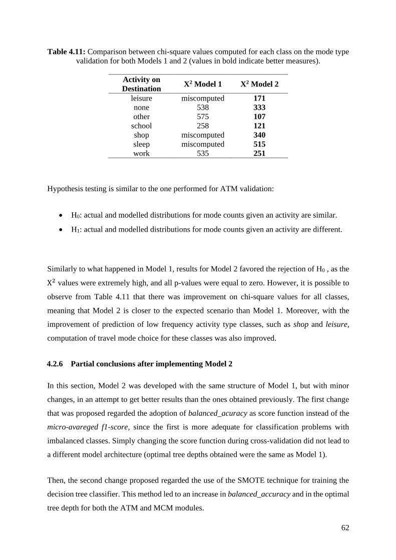
62

Table 4.11: Comparison between chi-square values computed for each class on the mode type

validation for both Models 1 and 2 (values in bold indicate better measures).

Activity on

Destination X2 Model 1 X2 Model 2

leisure miscomputed 171

none 538 333

other 575 107

school 258 121

shop miscomputed 340

sleep miscomputed 515

work 535 251




Similarly to what happened in Model 1, results for Model 2 favored the rejection of H0 , as the

Χ2 values were extremely high, and all p-values were equal to zero. However, it is possible to

observe from Table 4.11 that there was improvement on chi-square values for all classes,

meaning that Model 2 is closer to the expected scenario than Model 1. Moreover, with the

improvement of prediction of low frequency activity type classes, such as shop and leisure,

computation of travel mode choice for these classes was also improved.


In this section, Model 2 was developed with the same structure of Model 1, but with minor

changes, in an attempt to get better results than the ones obtained previously. The first change

that was proposed regarded the adoption of balanced_acuracy as score function instead of the

micro-avareged f1-score, since the first is more adequate for classification problems with

imbalanced classes. Simply changing the score function during cross-validation did not lead to

a different model architecture (optimal tree depths obtained were the same as Model 1).

Then, the second change proposed regarded the use of the SMOTE technique for training the

decision tree classifier. This method led to an increase in balanced_accuracy and in the optimal

tree depth for both the ATM and MCM modules.

63

Perhaps due to the increase on the size of the tree, overall feature importance for the ATM

module increased, although count features continued being not much important. Predicted

activity chains seemed more realistic in Model 2 than on Model 1, because of its higher

diversity. However, prediction of long and repetitive chains (a possible consequence of the low

importance of count features) contributed for a low overall validation score for the ATM

module. The adoption of ensemble tree models might address this issue.

The MCM module of Model 2 had a better performance than on Model 1 in both training and

test scores, which indicates that the SMOTE technique was useful.

4.3 MODEL 3: USING A RANDOM FOREST CLASSIFIER

4.3.1 Training results for Model 3

Based on the results obtained from Models 1 and 2, which indicated that some important

features were not having significant impact on the performance of the model, the ATM and

MCM modules were than trained as Random Forest classifiers in order to try achieving better

balanced accuracy scores. This approach is identified on this document as Model 3. Since the

SMOTE technique provided improvement on Model 2 in comparison to Model 1, it was again

adopted on the training phase of Model 3.

Cross-validation for the Random Forest models was conducted differently from what was done

in the Decision Tree models. Instead of running a 5-fold cross-validation for each possible tree

depth, in order to find the optimal tree depth, only one model for each possible max_depth

attribute was run, since for each run of the ensemble model, 100 different trees are created and

compared among each other.

Figure 4.16 presents the results obtained for cross-validation training of the Random Forest

classifier ATM module, and Figure 4.17 presents the same information for the MCM module.

Table 4.12 displays the optimal depths found by using the balanced accuracy score function.

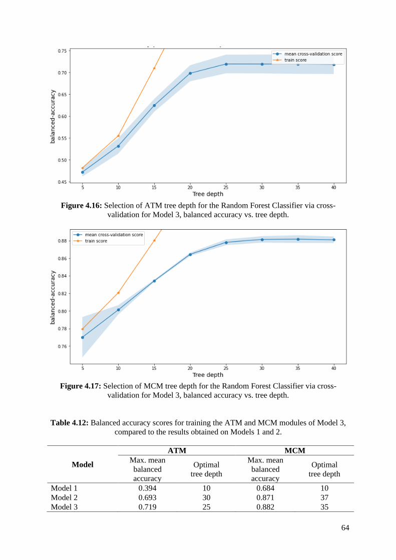
64

Figure 4.16: Selection of ATM tree depth for the Random Forest Classifier via cross-

validation for Model 3, balanced accuracy vs. tree depth.

Figure 4.17: Selection of MCM tree depth for the Random Forest Classifier via cross-

validation for Model 3, balanced accuracy vs. tree depth.


compared to the results obtained on Models 1 and 2.

Model

ATM MCM

Max. mean

balanced

accuracy

Optimal

tree depth

Max. mean

balanced

accuracy

Optimal

tree depth

Model 1 0.394 10 0.684 10

Model 2 0.693 30 0.871 37

Model 3 0.719 25 0.882 35

65

It can be concluded from the results on Table 4.12 that the adoption of Random Forest

Classifiers instead of Decision Tree Classifiers was able to improve the maximum balanced

accuracy on training of both the ATM and MCM modules. Moreover, optimal tree depths

obtained for Model 3 were slightly shallower than the ones found for Model 2, which is good

for avoiding overfitting.

In sequence, both ATM and MCM were trained as Random Forest Classifiers on the full

training set using the configuration that was obtained from cross-validation, including the

SMOTE technique. This training took 78 seconds to run on the on the cloud computational

environment Kaggle. Test results are presented on the next subsections.


After the training of the ATM and MCM modules as described in the previous subsection, the

models were run as part of the DDAS framework implementation that was described in

Chapter 3, using the test dataset (6868 agents). This implementation took 11 minutes and 7

seconds to run on the on the cloud computational environment Kaggle, considering that the

models were already trained.



Similarly to what was presented for the previous models, the first analysis that is conducted on

the results regards the expected (from the test set) and observed (model predictions) distribution

of trips. Figure 4.18 displays the comparison of results obtained for Models 1, 2 and 3. It is

possible to note that the prediction proportions of activity types for Model 3 are the closest to

the expected values that were obtained for all models evaluated in the current study.


A comparison between expected and observed frequencies of activity chains was conducted, in

order to evaluate Model 3 performance. Results for the 10 most frequent activity chains for

each result set are presented in Table 4.13.

66

Figure 4.18: Comparison between the expected and observed proportions (Models 1, 2 and 3)

of activity types on the agent’s schedules.


Type of

activity chain

Frequency on the

test dataset

(expected values)


Frequency on the

results dataset

(observed values)

HWH 2467 (36%) HWH 2531 (37%)

HOH 915 (13%) HSH 1046 (15%)

HSH 789 (11%) HOH 943 (14%)

HBH 347 (5%) HBH 738 (11%)

HOHOH 194 (3%) HLH 456 (7%)

HWHWH 185 (3% HOHWH 114 (2%)

HLH 155 (2%) HWHWH 106 (2%)

HOOH 79 (1%) HOHOH 101 (2%)

HWHOH 73 (1%) HOHOHOHOHOHOHH 83 (1%)

HWOH 69 (1%) HOHOHOH 56 (<1%)

Other patterns

(444 instances) 1595 (23%)

Other patterns

(123 instances) 694 (10%)


By observing the results presented in Table 4.13, it is possible to conclude that Model 3 appears

to be the most credible model developed in the current study with respect to the predicted

activity chains. Not only the actual most frequent activity chains are well represented in the

results of Model 3, but also there is a wide variety of schedules being predicted by the model.

Similarly to what was observed on the results of Model 2, some long and repetitive chains

appeared on the result list of predicted schedules for Model 3. However, Figure 4.19 indicates

that 13-trip chains are less frequent in the latter model (211 occurrences) than on the previous

one (945 occurrences).

67



Similarly to what was done on the analysis of results of Models 1 and 2, average values for the

permutation_importance function from Scikit-learn was computed to evaluate importance of

features in Model 3. Table 4.14 presents these results.

The information of whether the agent is at home or not is again on the top three most important

features of the classifier, and it is reasonable because all agents start at sleep, so there is a strong

indication to the model that the following activity, after sleep, should not be sleep again, neither

none. The features age_group, which was the most important feature of Model 2, and

people_in_household, which was also a feature of great importance on Model 2, complete the

Top 3 ranking of feature importance for Model 3.

Again, count features are not particularly important to the model (all features of that type have

importance values < 0.1), which may still be the cause for the prediction of some awfully long

activity chains. The adoption of an ensemble mode did not help solving this problem, that was

already evident in Model 2.

68

Table 4.14: Permutation importance for features of the ATM module in Models 1, 2 and 3.

Null values are highlighted in red color.

Feature Importance on

Model 1

Importance on

Model 2

Importance on

Model 3

is_origin_sleep 0.298876 0.360774 0.285347

age_group 0.020070 0.394552 0.263374

people_in_household 0.000084 0.297516 0.214096

education_level 0.005790 0.318535 0.193852

reach_bike 0.010492 0.382066 0.148993

is_female 0.010928 0.168500 0.132949

is_student 0.070084 0.126554 0.122529

has_driver_license 0.000317 0.178839 0.115733

reach_car 0.000942 0.238699 0.112085

reach_walk 0.000000 0.282089 0.102298

reach_transit 0.000041 0.217179 0.099807

is_origin_work 0.000000 0.099739 0.089153

is_car_available 0.000000 0.099509 0.076224

count_work 0.000022 0.086074 0.070164

is_origin_other 0.000068 0.071478 0.066914

count_other 0.000000 0.075894 0.050011

count_school 0.000000 0.045843 0.036623

is_origin_school 0.000000 0.032853 0.030420

count_sleep 0.000000 0.040117 0.026285

is_origin_shop 0.000000 0.018393 0.017241

count_shop 0.000000 0.012090 0.008411

is_origin_leisure 0.000000 0.007423 0.006955

count_leisure 0.000000 0.003654 0.002550





Table 4.15 presents a comparison between chi-square measures for Models 1, 2, and 3, for each

activity type.

The aim of the Pearson’s chi-square (Χ2) statistical test is to verify goodness of fit, or if an

observed frequency distribution is similar to a theoretical distribution. As described in Chapter

3, the objective of the current analysis is to determine if the real values (from the FDUMS

dataset) and the predicted distributions using the ATM module on Model 3 are statistically

different.

69


Table 4.15: Comparison between chi-square values computed for each class on the activity

type validation for Models 1, 2 and 3 (values in bold indicate better measures).

Activity Type X2 Model 1 X2 Model 2 X2 Model 3

leisure 376 479 134

other 888 3015 1303

school 91 25 8

shop 909 8273 447

sleep 1478 2809 454

work 1150 23111 1101

70

Hence, there are two hypotheses:



The results obtained for the Model 3, which are presented in Figure 4.20 favored the rejection

of H0, as almost all Χ2 values were extremely high, and correspondent p-values were equal to

zero. The exception was for the school activity type, which had a Χ2 = 8.99 with a

correspondent p-value of 6% for 4 classes.

Furthermore, results in Table 4.15 indicate that Model 3 had an overall validation metric better

than Models 1 and 2 on the test set, in addition to being more accurate on the training set as

well.






Results are presented in Figure 4.21 and Table 4.16 displays a comparison between the chi-

square values obtained from Models 1, 2 and 3.




Similarly to what happened in Models 1 and 2, results for Model 3 favored the rejection of H0,

as the Χ2 values were extremely high, and all p-values were equal to zero. However, it is

possible to observe from Table 4.16 that there was improvement on chi-square values for all

classes, meaning that Model 3 is closer to the expected scenario than Models 1 and 2.

71


72

Table 4.16: Comparison between chi-square values computed for each class on the travel

mode choice validation for Models 1, 2 and 3 (values in bold indicate better measures).

Activity on

Destination X2 Model 1 X2 Model 2 X2 Model 3

leisure miscomputed 171 98

none 538 333 178

other 575 107 75

school 258 121 70

shop miscomputed 340 140

sleep miscomputed 515 184

work 535 251 113


In this section, Model 3 was developed with the same structure of Model 2 but using a Random

Forest Classifier as predictor for both the ATM and MCM modules, instead of the Decision

Tree Classifier that was used in Models 1 and 2. It was clear that Model 3 produced better

results on the training and test phases, for both the ATM and MCM modules, being its results

closer to what was expected than what was obtained in the previous models. This result

indicates that the adoption of the SMOTE technique on training and the Random Forest

Classifier as predictor are good improvements to be incorporated on the DDAS framework

4.4 SUMMARY OF RESULTS

Table 4.17 presents a summary of the results that have been presented in this chapter.

Table 4.17: Summary of the results of the current study.

Attribute Original

DDAS Model 1 Model 2 Model 3

Training results

ATM max. balanced accuracy not informed 0.394 0.693 0.719

ATM optimal tree depth 6 10 30 25

MCM max. balanced accuracy not informed 0.684 0.871 0.882

MCM optimal tree depth 8 10 37 35

Time for training the modules* not informed 1.1” 9.6” 78.2”

General test results

Time for running the framework* not informed 3’27” 6’12” 11’7”

Total X2 for both ATM and MCM not informed 6758 39556 4305

73

Table 4.17 (Cont): Summary of the results of the current study.

Attribute Original

DDAS Model 1 Model 2 Model 3

ATM validation results

X2 for activity leisure 538 376 479 134

X2 for activity other N/A 888 3015 1303

X2 for activity school not informed 91 25 8

X2 for activity shop 7374 909 8273 447

X2 for activity sleep not informed 1478 2809 454

X2 for activity work not informed 1150 23111 1101

Total X2 for all activities not informed 4893 37716 3447

MCM validation results

X2 for destination leisure 22740 mis-

computed 171 98

X2 for destination none not informed 538 333 178

X2 for destination other N/A 575 107 75

X2 for destination school 30440 258 121 70

X2 for destination shop 23940 mis-

computed 340 140

X2 for destination sleep 145200 mis-

computed 515 184

X2 for destination work 19240 535 251 113

Total X2 for all destinations not informed 1865 1840 858

74

5 CONCLUSIONS AND RECOMMENDATIONS

5.1 CONCLUSIONS

The aim of this research was to develop a commented replication of two modules of the Data-

Driven Activity Scheduler (DDAS) framework proposed by Drchal et al. (2019) for an activity-

based transportation model: the Activity Type Model (ATM) and the Mode Choice Model

(MCM). In order to achieve this aim, three objectives have been defined. The first one regarded

the replication of the ATM and MCM modules using travel data available for the Metropolitan

Region of Brasilia in the Federal District Urban Mobility Survey (FDUMS). The procedures

and results related to this replication were identified in the current document as Model 1.

After cleansing, the FDUMS tables provided information about 92,696 trips performed by

34,340 agents within a working day, which represents an input set more than 13 times larger

than the one that was used by Drchal et al. (2019). The authors of DDAS have indicated that

one of the limitations of their study was the small size of the dataset available for their proof-

of-concept, and they expected to achieve better results with larger training sets of data. Indeed,

the current replication of the DDAS modules produced better validation metrics for both ATM

and MCM, as can be observed in Table 4.17, considering the VALFRAM validation

framework. Moreover, Model 1 produced better results for travel mode choice prediction,

compared to the ones reported by Drchal et al. (2019) even without the hard coded rules that

were implemented in the original DDAS, such as only allowing the prediction of mode car for

these agents who had it available in their homes. It could be concluded that the model was able

to learn these patterns by itself.

The second objective of this study concerned the investigation of possible improvements to be

made on the DDAS framework, especially on the ATM and MCM modules, which were being

implemented. This task was performed in the course of the development of Model 1.

During the phase of training the models, the first result that draw attention was the F1-score

obtained for the ATM module, which was 26% lower than the one presented in the DDAS

paper. Since the current implementation had an input dataset more than 13 times larger, it was

expected that the training accuracy of the models improved. It was concluded, then, that perhaps

75

the F1-score was not the best choice for accuracy measurement for ATM and MCM, which had

input datasets with imbalanced class proportions on prediction, and other measurements such

as the balanced accuracy score (also called macro-averaged recall) could be a better indicator

in this scenario. Another minor issue that was noted during Model 1 implementation was the

lack of detail presented by Drchal et al. (2019) regarding training of the DDAS modules.

Resources such as confusion matrices and reports of accuracy measures would be useful for

analyzing the framework, but they were not reported in the DDAS paper. The current research

filled this gap by providing this information for Model 1.

In the validation phase of Model 1, other potential improvements to DDAS were identified,

especially regarding the VALFRAM framework. The activity count validation metric, which is

based on the comparison of expected and observed counts of schedules having 1, 2, 3…

occurrences of a certain activity type, was proven to be weak in terms of indicating how close

to reality are the predicted results. In Model 1, for instance, no activities of types leisure or

sleep were predicted, and due to the manner how VALFRAM is designed, these classes had no

contribution in decreasing the evaluation score for the model (chi-square values for these

classes were equal to zero). It was concluded that travel mode choice validation also had

indications that it was faulty as it depended on the results of activity type prediction.

Moreover, both methodologies that are part of VALFRAM for validating the ATM and MCM

modules rely on aggregate metrics, which is incompatible to the whole principle of disaggregate

activity-based models. Perhaps individual measurements for each agent would be more useful

for transportation planning. For instance, given an agent with a real chain home-work-leisure-

home, performing all trips by car, significant validation measurements would include if the

model is able to predict that this specific agent performs at least one activity of type work or at

least one activity of type leisure. It would be also important to check if the model can predict

that this agent performs three trips during a day, and that all trips have the transportation mode

car. None of this information is being checked by the VALFRAM framework.

The third objective was the implementation and evaluation of the potential improvements that

had been identified while replicating the DDAS framework. Therefore, two different

implementations were tested: the first one (Model 2) included the balanced accuracy score for

cross-validation metric and the Synthetic Minority Over-Sampling Technique (SMOTE), to

synthetically balance the activity type classes; the second implementation (Model 3) was similar

76

to Model 2, but used a Random Forest classifier instead of the Decision Tree classifier that

composed Models 1, 2 and the original DDAS.

It was concluded that both Models 2 and 3 produced better validation results (VALFRAM

scores) for the MCM module, and better training scores for both ATM and MCM. Nevertheless,

Model 3 stood out by producing better VALFRAM scores for the ATM module as well, in

addition to generating more reasonable activity chains, with little increase in computation time.

It can be said that Model 3, designed and trained as it is, may be a useful tool for transportation

planning within the Metropolitan Area of Brasilia. The only input data needed for predicting

activity schedules with activity chains and travel mode choice are the socio-demographic

characteristics of the agents, information that is collected biannually by the Federal District

Planning Company (Companhia de Planejamento do Distrito Federal – CODEPLAN).

In conclusion, there is still improvement to be made to Model 3, especially regarding the small

portion of prediction of long and repetitive chains by the ATM module. However, the full public

availability of all Python code developed in the course of the current research, which was the

fourth and final objective of this study, must encourage further investigation and faster

advancements on the transport modeling field.

5.2 LIMITATIONS OF THE STUDY

One of the limitations of the current study regarded the difficulty in classifying activity and

mode types in order to make them compatible to the classes specified in the DDAS paper. It

was not possible to assure that the same methodology for classifying activity types was used in

the FDUMS datasets and in the input data used that was used by Drchal et al. (2019), as none

of the publications have detailed their classification procedures. It is clear that some overlap

may occur between leisure and shop activity types, and an example is the activity eating out

that was part of the FDUMS dataset. Moreover, activity and mode types on the FDUMS dataset

were much more complex than what was presented in the DDAS paper. The FDUMS dataset

included for instance an activity type taking someone somewhere, and mode types motorcycle

as driver, motorcycle as passenger, private charter, none of them having correspondence on

the DDAS framework classes.

77

Another limitation of the study was the absence of a feature indicating if each person had or not

a public transportation card in the FDUMS dataset. This was the only feature required by the

original DDAS implementation that was not available on the input of the current research.

5.3 RECOMMENDATIONS FOR FUTURE RESEARCH

Based on the findings of the current study, the following opportunities for technical and

academic advances are recommended for future research:

• Creating a critical analysis regarding the other two modules of DDAS (Activity

Duration Model and Activity Attractor Model).

• Assessing the incorporation more features on training the ATM and MCM modules,

such as the location (administrative region) where each person lives, not only to try to

achieve better performance, but also to provide more useful insights for transportation

planning.

• Evaluating the adoption of different machine learning algorithms on the DDAS

modules, such as a long term short-memory (LTSM) predictor for the ATM module, as

that could incorporate the effects of activity chaining, and neural networks for the MCM

module, as it is proved to be a good classifier for travel mode choice models.

• Developing a new validation framework for activity-based models that considers the

results obtained from each individual agent, differently to VALFRAM, that computes

aggregate measurements.

• Incorporating the proposed model into a tool for urban and mobility planning for the

region of the Federal District.

78

REFERENCES

Abdulazim, T., Abdelgawad, H., Habib, K., e Abdulhai, B. (2013) Using smartphones and

sensor technologies to automate collection of travel data. Transportation Research

Record, (2383), 44–52. doi:10.3141/2383-06

Abduljabbar, R., Dia, H., Liyanage, S., e Bagloee, S. A. (2019) Applications of artificial

intelligence in transport: An overview. Sustainability (Switzerland), 11(1).

doi:10.3390/su11010189

Allahviranloo, M., e Recker, W. (2013) Daily activity pattern recognition by using support

vector machines with multiple classes. Transportation Research Part B: Methodological,

58, 16–43. doi:10.1016/j.trb.2013.09.008

Alves, V. F. B. (2011) Explorando Técnicas para a Localização e Identificação de Potenciais

Usuários de Transporte Público Urbano. Master's Thesis. Universidade de São Paulo.

Anchante, J. T. (2017) Commute mode choice in the city of São Paulo: an empirical analysis.

Master's Thesis. Universidade Federal de Viçosa.

Arentze, T., e Timmermans, H. (2004) A learning-based transportation oriented simulation

system. Transportation Research Part B: Methodological, 38(7), 613–633.

doi:10.1016/j.trb.2002.10.001

Arruda, F. S. (2005) Aplicação de um modelo baseado em atividades para analise da relação

uso do uso e transportes no contexto brasileiro. Ph.D. Dissertation. Universidade de São

Paulo.

Aschwanden, G. D. P. A., Wijnands, J. S., Thompson, J., Nice, K. A., Zhao, H., e Stevenson,

M. (2019) Learning to walk: Modeling transportation mode choice distribution through

neural networks. Environment and Planning B: Urban Analytics and City Science, 0(0),

1–14. doi:10.1177/2399808319862571

Assi, K. J., Nahiduzzaman, K. M., Ratrout, N. T., e Aldosary, A. S. (2018) Mode choice

behavior of high school goers: Evaluating logistic regression and MLP neural networks.

Case Studies on Transport Policy, 6(2), 225–230. doi:10.1016/j.cstp.2018.04.006

Assi, K. J., Shafiullah, M., Nahiduzzaman, K. M., e Mansoor, U. (2019) Travel-to-school mode

choice modelling employing artificial intelligence techniques: A comparative study.

Sustainability (Switzerland), 11(16). doi:10.3390/su11164484

Auld, J., e Mohammadian, A. (2009) Framework for the development of the agent-based

dynamic activity planning and travel scheduling (ADAPTS) model. Transportation

Letters, 1(3), 245–255. doi:10.3328/TL.2009.01.03.245-255

79

Barbosa, R. R. (2014) Análise da Dependência Espacial da Mobilidade Urbana do Idoso:

Aplicação aos Dados da Pesquisa Domiciliar de 2007 da Região Metropolitana de São

Paulo. Master's Thesis. Universidade de Brasília.

Beckman, J. D., e Goulias, K. G. (2008) Immigration, residential location, car ownership, and

commuting behavior : a multivariate latent class analysis from California. Transportation,

35, 655–671. doi:10.1007/s11116-008-9172-x

Bhat, C. R., Guo, J. Y., Srinivasan, S., e Sivakumar, A. (2004) Microsimulator for Daily

Activity-Travel Patterns. Transportation Research Record, 1894, 57–66.

Bowman, J. L., e Ben-Akiva, M. E. (2001) Activity-based disaggregate travel demand model

system with activity schedules. Transportation Research Part A: Policy and Practice,

35(1), 1–28. doi:10.1016/S0965-8564(99)00043-9

Breiman, L., Friedman, J. H., Olshen, R. A., e Stone, C. J. (1984) Classification and Regression

Trees. Chapman & Hall/CRC, New York.

Breiman, Leo. (2001) Random Forests. Machine Learning, 45, 5–32.

doi:10.1201/9780367816377-11

Cantarella, G. E., e de Luca, S. (2005) Multilayer feedforward networks for transportation mode

choice analysis: An analysis and a comparison with random utility models. Transportation

Research Part C: Emerging Technologies, 13(2), 121–155. doi:10.1016/j.trc.2005.04.002

Cascetta, E. (2009) Transportation Systems Analysis: Models and Applications. (2o ed).

Springer US. doi:10.1007/978-0-387-75857-2

Chang, X., Wu, J., Liu, H., Yan, X., Sun, H., e Qu, Y. (2019) Travel mode choice: a data fusion

model using machine learning methods and evidence from travel diary survey data.

Transportmetrica A: Transport Science, 15(2), 1587–1612.

doi:10.1080/23249935.2019.1620380

Chapleau, R., Gaudette, P., e Spurr, T. (2019) Application of Machine Learning to Two Large-

Sample Household Travel Surveys: A Characterization of Travel Modes. Transportation

Research Record, 2673(4), 173–183. doi:10.1177/0361198119839339

Charypar, D., e Nagel, K. (2005) Generating complete all-day activity plans with genetic

algorithms. Transportation, 32(4), 369–397. doi:10.1007/s11116-004-8287-y

Chawla, N. V., Japkowicz, N., e Kotcz, A. (2004) Editorial. ACM SIGKDD Explorations

Newsletter, 6(1), 1–6. doi:10.1145/1007730.1007733

Cheng, L., Chen, X., De Vos, J., Lai, X., e Witlox, F. (2019) Applying a random forest method

approach to model travel mode choice behavior. Travel Behaviour and Society,

14(September 2018), 1–10. doi:10.1016/j.tbs.2018.09.002

80

Companhia do Metropolitano do Distrito Federal. ([s.d.]) PDTT-DF. Accessed in May 13,

2020, Retrieved from http://www.metro.df.gov.br/?page_id=40044

Companhia do Metropolitano do Distrito Federal. (2018) PDTT/DF - Plano de

Desenvolvimento do Transporte Público sobre Trilhos do Distrito Federal - Relatório

Final. Brasilia, Brazil. Retrieved from:

http://www.metro.df.gov.br/arquivos/relatorios_finais_PDTT_PMU.rar

Costa, A. S. G. da. (2013) Proposta de um Método para Estimação de Escolha Modal através

da Geoestatística. Master's Thesis. Universidade Federal da Bahia.

Cui, Y., Meng, C., He, Q., e Gao, J. (2018) Forecasting current and next trip purpose with social

media data and Google Places. Transportation Research Part C: Emerging Technologies,

97(September), 159–174. doi:10.1016/j.trc.2018.10.017

Dalmaso, R. C. (2009) Identificação e caracterização de grupos de indivíduos segundo padrões

de seqüências de atividades multidimensionais. Master's Thesis. Universidade de São

Paulo.

Deus, L. R. (2008) A influência da forma urbana no comportamento de viagem das pessoas:

Estudo de caso em Uberlândia, MG. Master's Thesis. Universidade Federal de São Carlos.

Diana, M., e Ceccato, R. (2019) A multimodal perspective in the study of car sharing switching

intentions. Transportation Letters, 00(00), 1–7. doi:10.1080/19427867.2019.1707351

Dong, X., Ben-Akiva, M. E., Bowman, J. L., e Walker, J. L. (2006) Moving from trip-based to

activity-based measures of accessibility. Transportation Research Part A: Policy and

Practice, 40(2), 163–180. doi:10.1016/j.tra.2005.05.002

Drchal, J., Čertický, M., e Jakob, M. (2016) VALFRAM: Validation framework for activity-

based models. Jasss, 19(3). doi:10.18564/jasss.3127

Drchal, J., Čertický, M., e Jakob, M. (2019) Data-driven activity scheduler for agent-based

mobility models. Transportation Research Part C: Emerging Technologies, 98(December

2018), 370–390. doi:10.1016/j.trc.2018.12.002

Ettema, D. (1996) Activity-based travel demand modeling (Tese de Doutorado). Technische

Universiteit Eindhoven.

Feng, T., e Timmermans, H. J. P. (2016) Comparison of advanced imputation algorithms for

detection of transportation mode and activity episode using GPS data. Transportation

Planning and Technology, 39(2), 180–194. doi:10.1080/03081060.2015.1127540

Garling, T., Kwan, M.-P., e Golledge, R. (1994) Computational-Process Household Activity

Modelling. Transportation Research Part B, 28B(5), 355–364.

81

Ghasri, M., Hossein Rashidi, T., e Waller, S. T. (2017) Developing a disaggregate travel

demand system of models using data mining techniques. Transportation Research Part A:

Policy and Practice, 105(June 2016), 138–153. doi:10.1016/j.tra.2017.08.020

Gogate, V., Dechter, R., Bidyuk, B., Rindt, C., e Marca, J. (2005) Modeling Transportation

Routines using Hybrid Dynamic Mixed Networks. Proceedings of the conference on

uncertainty in artificial intelligence. Edimburgh, Scotland.

Golshani, N., Shabanpour, R., Mahmoudifard, S. M., Derrible, S., e Mohammadian, A. (2018)

Modeling travel mode and timing decisions: Comparison of artificial neural networks and

copula-based joint model. Travel Behaviour and Society, 10(May 2017), 21–32.

doi:10.1016/j.tbs.2017.09.003

Grady, K. E. O., e Medoff, D. R. (1988) Multivariate Behavioral Categorical Variables in

Multiple Regression : Some Cautions. Multivariate Behavioral Research, 23(2), 243–260.

doi:10.1207/s15327906mbr2302

Gu, Q., Zhu, L., e Cai, Z. (2009) Evaluation measures of the classification performance of

imbalanced data sets. Communications in Computer and Information Science, 51, 461–

471. doi:10.1007/978-3-642-04962-0_53

Ha, T. V., Asada, T., e Arimura, M. (2019) Determination of the influence factors on household

vehicle ownership patterns in Phnom Penh using statistical and machine learning methods.

Journal of Transport Geography, 78(May), 70–86. doi:10.1016/j.jtrangeo.2019.05.015

Hafezi, M. H., Liu, L., e Millward, H. (2018) Learning Daily Activity Sequences of Population

Groups using Random Forest Theory. Transportation Research Record, 2672(47), 194–

207. doi:10.1177/0361198118773197

Hafezi, M. H., Liu, L., e Millward, H. (2019) A time-use activity-pattern recognition model for

activity-based travel demand modeling. Transportation, 46(4), 1369–1394.

doi:10.1007/s11116-017-9840-9

Hafezi, M. H., Millward, H., e Liu, L. (2018) Acitivity-Based Travel Demand Modeling:

Progress and Possibilities. International Conference on Transportation and Development

(p. 138–147). Transportation & Development of ASCE, Pittsburgh, Pennsylvania. Obtido

de http://www.asce-ictd.org/

Hagenauer, J., e Helbich, M. (2017) A comparative study of machine learning classifiers for

modeling travel mode choice. Expert Systems with Applications, 78, 273–282.

doi:10.1016/j.eswa.2017.01.057

Hastie, T., Tibshirani, R., e Friedman, J. (2009) The Elements of Statistical Learning: Data

Mining, Inference, and Prediction. Encyclopedia of Systems Biology (2o ed). Springer,

New York. doi:10.1007/978-1-4419-9863-7_941

82

Hensher, D. A., e Ton, T. T. (2000) A comparison of the predictive potential of artificial neural

networks and nested logit models for commuter mode choice. Transportation Research

Part E: Logistics and Transportation Review, 36(3), 155–172. doi:10.1016/S1366-

5545(99)00030-7

Hossin, M., e Sulaiman, M. . (2015) A Review on Evaluation Metrics for Data Classification

Evaluations. International Journal of Data Mining & Knowledge Management Process,

5(2), 01–11. doi:10.5121/ijdkp.2015.5201

Hussain, H. D., Mohammed, A. M., Salman, A. D., Rahmat, R. A. B. O. K., e Borhan, M. N.

(2017) Analysis of transportation mode choice using a comparison of artificial neural

network and multinomial logit models. ARPN Journal of Engineering and Applied

Sciences, 12(5), 1483–1493.

IBGE. ([s.d.]) Sinopse do Censo Demográfico 2010 - Distrito Federal. Obtido 30 de agosto de

2020, de https://censo2010.ibge.gov.br/sinopse/index.php?uf=53&dados=1

Ichikawa, S. M. (2002) Aplicação de Minerador de Dados na Obtenção de Relações entre

Padrões de Encadeamento de Viagens Condificados e Características Socio-econômicas.

Master's Thesis. Universidade de São Paulo.

Kato, K., Matsumoto, S., e Sano, K. (2002) Microsimulation for commuters’ mode and

discretionary activities by using neural networks. Proceedings of the Conference on

Traffic and Transportation Studies, ICTTS, (2002), 1290–1297.

doi:10.1061/40630(255)178

Kitamura, R., Pas, E. I., Lula, C. V., Keith Lawton, T., e Benson, P. E. (1996) The sequenced

activity mobility simulator (SAMS): An integrated approach to modeling transportation,

land use and air quality. Transportation, 23(3), 267–291. doi:10.1007/BF00165705

Kotsiantis, S. B. (2007) Supervised Machine Learning: A Review of Classification Techniques.

Informatica, (31), 249–268.

Koushik, A. N. P., Manoj, M., e Nezamuddin, N. (2020) Machine learning applications in

activity-travel behaviour research: a review. Transport Reviews, 40(3), 288–311.

doi:10.1080/01441647.2019.1704307

Krempels, K. H., Ohler, F., Osterland, T., e Terwelp, C. (2019) Context-based user activity

prediction for mobility planning. ICAART 2019 - Proceedings of the 11th International

Conference on Agents and Artificial Intelligence, 2, 568–575.

doi:10.5220/0007351105680575

Kwan, M.-P. (1997) GISICAS: An activity-based travel decision support system using a GIS-

interfacesd computational-process model. Activity-based Approaches to Travel Analysis

(p. 279–282). Pergamon, Oxford.

83

Lee, D., Derrible, S., e Pereira, F. C. (2018) Comparison of Four Types of Artificial Neural

Network and a Multinomial Logit Model for Travel Mode Choice Modeling.

Transportation Research Record, 2672(49), 101–112. doi:10.1177/0361198118796971

Li, X., Li, H., e Xu, X. (2018) A Bayesian network modeling for departure time choice: A case

study of beijing subway. Promet - Traffic - Traffico, 30(5), 579–587.

doi:10.7307/ptt.v30i5.2644

Li, Z., Wang, W., Yang, C., e Ragland, D. R. (2013) Bicycle commuting market analysis using

attitudinal market segmentation approach. Transportation Research Part A: Policy and

Practice, 47, 56–68. doi:10.1016/j.tra.2012.10.017

Lin, H., Lo, H., e Chen, X. (2009) Lifestyle classifications with and without activity-travel

patterns. Transportation Research Part A, 43(6), 626–638. doi:10.1016/j.tra.2009.04.002

Lindner, A., Pitombo, C. S., e Cunha, A. L. (2017) Estimating motorized travel mode choice

using classifiers: An application for high-dimensional multicollinear data. Travel

Behaviour and Society, 6, 100–109. doi:10.1016/j.tbs.2016.08.003

Ma, T. Y. (2015) Bayesian networks for multimodal mode choice behavior modelling: A case

study for the cross border workers of Luxembourg. Transportation Research Procedia,

10(July), 870–880. doi:10.1016/j.trpro.2015.09.040

Ma, T. Y., Chow, J. Y. J., e Xu, J. (2017) Causal structure learning for travel mode choice using

structural restrictions and model averaging algorithm. Transportmetrica A: Transport

Science, 13(4), 299–325. doi:10.1080/23249935.2016.1265019

Ma, T. Y., e Klein, S. (2018) Bayesian networks for constrained location choice modeling using

structural restrictions and model averaging. European Journal of Transport and

Infrastructure Research, 18(1), 91–111. doi:10.18757/ejtir.2018.18.1.3221

Ma, X., Wu, Y. J., Wang, Y., Chen, F., e Liu, J. (2013) Mining smart card data for transit riders’

travel patterns. Transportation Research Part C: Emerging Technologies, 36, 1–12.

doi:10.1016/j.trc.2013.07.010

Mäenpää, H., Lobov, A., e Martinez Lastra, J. L. (2017) Travel mode estimation for multi-

modal journey planner. Transportation Research Part C: Emerging Technologies, 82,

273–289. doi:10.1016/j.trc.2017.06.021

Medrano, R. M. A. (2012) Modelagem de padrões de viagens e expansão urbana. Master's

Thesis. Universidade de Brasília.

Miller, E. J., e Roorda, M. J. (2003) Prototype Model of Household Activity-Travel Scheduling.

Transportation Research Record, (1831), 114–121.

Minal, S., Sekhar, C. R., e Madhu, E. (2019) Development of neuro-fuzzy-based multimodal

84

mode choice model for commuter in Delhi. IET Intelligent Transport Systems, 13(2), 406–

416. doi:10.1049/iet-its.2018.5112

Miranda, D. (2020) Urban Mobility Survey (Federal District, Brazil). Kaggle.

doi:10.34740/kaggle/dsv/1315731

Mohammadian, A., e Miller, E. J. (2002) Nested Logit Models and Artificial Neural Networks

for Predicting Household Automobile Choices Comparison of Performance.

Transportation Research Record, 1807, 92–100.

Murphy, K. P. (2012) Machine Learning: A Probabilistic Perspective. The MIT Press, London,

England.

Omrani, H., Charif, O., Gerber, P., Awasthi, A., e Trigano, P. (2013) Prediction of individual

travel mode with evidential neural network model. Transportation Research Record,

(2399), 1–8. doi:10.3141/2399-01

Ortúzar, J. de D., e Willumsen, L. G. (2011) Modelling Transport. (4th editio.). John Wiley &

Sons.

Paiva Junior, H. de. (2006) Segmentação e modelagem comportamental de usuários dos

serviços de transporte urbano brasileiros. Ph.D. Dissertation. Universidade de São Paulo.

Paredes, M., Hemberg, E., O’Reilly, U. M., e Zegras, C. (2017) Machine learning or discrete

choice models for car ownership demand estimation and prediction? 5th IEEE

International Conference on Models and Technologies for Intelligent Transportation

Systems, MT-ITS 2017 - Proceedings, 780–785. doi:10.1109/MTITS.2017.8005618

Park, J. J., Park, D.-S., Jeong, Y.-S., e Pan, Y. (2018) Advances in Computer Science and

Ubiquitous Computing. Springer, Singapore. doi:10.5772/172

Pedregosa, F., Varoquaux, G., Gramfort, A., Michel, V., e Thirion, B. (2011) Scikit-learn:

Machine Learning in Pyhton. Journal of Machine Learning Reseach, (12), 2825–2830.

doi:10.1145/2786984.2786995

Pirra, M., e Diana, M. (2016) Classification of tours in the U.S. National household travel

survey through clustering techniques. Journal of Transportation Engineering, 142(6).

doi:10.1061/(ASCE)TE.1943-5436.0000845

Pirra, M., e Diana, M. (2019) A study of tour-based mode choice based on a Support Vector

Machine classifier. Transportation Planning and Technology, 42(1), 23–36.

doi:10.1080/03081060.2018.1541280

Pitombo, C. S. (2003) Análise do comportamento subjacente ao encadeamento de viagens

através do uso minerador de dados. Master's Thesis. Universidade de São Paulo.

85

Pitombo, C. S. (2007) Estudos de relações entre variáveis socioeconômicas, de uso do solo,

participação em atividades e padrões de viagens encadeadas urbanas. Ph.D. Dissertation.

Universidade de São Paulo.

Pitombo, C. S., Bertocini, B. V., e Kawamoto, E. (2008) An application of exploratory

multivariate data analysis techniques in a peer study of land use influence on individual

destination choices. Proceedings of the 11th IEEE International Conference on

Computational Science and Engineering, CSE Workshops 2008, 59–64.

doi:10.1109/CSEW.2008.20

Pitombo, C. S., Kawamoto, E., e Sousa, A. J. (2011) An exploratory analysis of relationships

between socioeconomic , land use , activity participation variables and travel patterns.

Transport Policy, 18(2), 347–357. doi:10.1016/j.tranpol.2010.10.010

Přibyl, O., e Goulias, K. G. (2005) Simulation of daily activity patterns incorporating

interactions within households: Algorithm overview and performance. Transportation

Research Record, 2003(1926), 135–141. doi:10.3141/1926-16

Pronello, C., e Camusso, C. (2011) Travellers’ profiles definition using statistical multivariate

analysis of attitudinal variables. Journal of Transport Geography, 19(6), 1294–1308.

doi:10.1016/j.jtrangeo.2011.06.009

Quinlan, J. R. (1986) Induction of decision trees. Machine Learning, 1(1), 81–106.

doi:10.1007/bf00116251

Quinlan, J. R. (1993) C4.5: Programs for Machine Learning. Morgan Kaufmann, San Mateo.

doi:10.1007/BF00993309

Rakha, T., Rose, C. M., e Reinhart, C. F. (2014) A framework for modeling occupancy

schedules and local trips based on activity based surveys. Building Simulation Conference

(p. 433–440). ASHRA E/IBPSA-USA, Atlanta.

Recker, W. W., McNally, M. G., e Root, G. S. (1986) A model of complex travel behavior: Part

I-Theoretical development. Transportation Research Part A: General, 20(4), 307–318.

doi:10.1016/0191-2607(86)90089-0

Ribeiro, M. D. (2014) Tecnologia GPS em pesquisa de origem e destino. Master's Thesis.

Universidade Federal do Rio Grande do Sul.

Rodrigues, J. G. P., Pereira, J. P., e Aguiar, A. (2017) Impact of Crowdsourced Data Quality

on Travel Pattern Estimation. Proceedings of First ACM Workshop on Mobile

Crowdsensing Systems and Applications (CrowdSenSys’17). ACM, New York.

Roorda, M., Miller, E. J., e Kruchten, N. (2006) Incorporating within-household interactions

into mode choice model with genetic algorithm for parameter estimation. Transportation

Research Record, (1985), 171–179. doi:10.3141/1985-19

86

Scikit-learn User Guide. (2020a) 1.10. Decision Trees. Obtido 23 de maio de 2020, de

https://scikit-learn.org/stable/modules/tree.html#minimal-cost-complexity-pruning

Scikit-learn User Guide. (2020b) 6.3. Preprocessing data. Obtido 24 de maio de 2020, de

https://scikit-learn.org/stable/modules/preprocessing.html

Shalev-Shwartz, S., e Ben-David, S. (2013) Understanding machine learning: From theory to

algorithms. Understanding Machine Learning: From Theory to Algorithms (Vol.

9781107057). doi:10.1017/CBO9781107298019

Shmueli, D., Salomon, I., e Shefer, D. (1996) Neural network analysis of travel behavior:

evaluating tools for prediction. Transportation Research Part C: Emerging Technologies,

4(3), 151–166.

Silva, D. C. (2017) Violence, security perception and mode choice on trips to and from a

university campus. Universidade de São Paulo.

Silva, M. A. e. (2006) Verificação Da Aplicabilidade Da Técnica De Mineração De Dados Na

Previsão Da Demanda Por Transporte De Passageiros Urbanos Usando Dados Da

Região Metropolitana De São Paulo. Master's Thesis. Universidade de São Paulo.

Silva, T. (2010) Análise Da Escolha Modal Binomial Com Base No Modelo Logit. Master's

Thesis. Universidade Federal de Uberlândia.

Sokolova, M., e Lapalme, G. (2009) A systematic analysis of performance measures for

classification tasks. Information Processing and Management, 45(4), 427–437.

doi:10.1016/j.ipm.2009.03.002

Sousa, P. B. de. (2004) Análise comparativa do encadeamento de viagens de três áreas

urbanas. Master's Thesis. Universidade de São Paulo.

Stenneth, L., Wolfson, O., Yu, P. S., e Xu, B. (2011) Transportation mode detection using

mobile phones and GIS information. GIS: Proceedings of the ACM International

Symposium on Advances in Geographic Information Systems, 54–63.

doi:10.1145/2093973.2093982

Sun, B., e Park, B. B. (2017) Route choice modeling with Support Vector Machine.

Transportation Research Procedia, 25, 1806–1814. doi:10.1016/j.trpro.2017.05.151

Taco, P. W. G. (2003) Redes Neurais Artificiais Aplicadas na Modelagem Individual de

Padrões de Viagens Encadeadas a Pé. Ph.D. Dissertation. Universidade de São Paulo.

Tang, L., Xiong, C., e Zhang, L. (2018) Spatial Transferability of Neural Network Models in

Travel Demand Modeling. Journal of Computing in Civil Engineering, 32(3), 1–10.

doi:10.1061/(ASCE)CP.1943-5487.0000752

87

Tavares, A. R., e Bazzan, A. L. C. (2012) Reinforcement learning for route choice in an abstract

traffic scenario. VI Workshop-Escola de Sistemas de Agentes, seus Ambientes e aplicações

(WESAAC), 141–153.

Thill, J., e Wheeler, A. (2000) Tree Induction of Spatial Choice Behavior. Transportation

Research Record, 1719, 250–258.

Van Asch, V. (2013) Macro-and micro-averaged evaluation measures. Computational

Linguistics & Psicolinguistics (CLiPs). Antwep. Obtido de

https://www.clips.uantwerpen.be/~vincent/pdf/microaverage.pdf

Vanhulsel, M., Janssens, D., Wets, G., e Vanhoof, K. (2009) Simulation of sequential data: An

enhanced reinforcement learning approach. Expert Systems with Applications, 36(4),

8032–8039. doi:10.1016/j.eswa.2008.10.056

Verhoeven, M., Arentze, T., Timmermans, H., e Van Der Waerden, P. (2007) Simulating the

influence of life trajectory events on transport mode behavior in an agent-based system.

IEEE Conference on Intelligent Transportation Systems, Proceedings, ITSC, 107–112.

doi:10.1109/ITSC.2007.4357815

Vovsha, P., Petersen, E., e Donnelly, R. (2002) Microsimulation in travel demand modeling:

Lessons learned from the New York best practice model. Transportation Research Record,

(1805), 68–77. doi:10.3141/1805-09

Wang, B., Gao, L., e Juan, Z. (2017) Travel Mode Detection Using GPS Data and

Socioeconomic Attributes Based on a Random Forest Classifier. IEEE Transactions on

Intelligent Transportation Systems, 1–12.

Wang, L., Ma, W., Fan, Y., e Zuo, Z. (2017) Trip chain extraction using smartphone-collected

trajectory data. Transportamerica B: Transport Dynamics, (October).

doi:10.1080/21680566.2017.1386599

Wang, Q., Sun, H., e Zhang, Q. (2017) A Bayesian Network Model on the Public Bicycle

Choice Behavior of Residents: A Case Study of Xi’an. Mathematical Problems in

Engineering, 2017(4), 16–18. doi:10.1155/2017/3023956

Wei, F., Ma, S., e Jia, N. (2014) A day-to-day route choice model based on reinforcement

learning. Mathematical Problems in Engineering, 2014. doi:10.1155/2014/646548

Weng, J., Tu, Q., Yuan, R., Lin, P., e Chen, Z. (2018) Modeling mode choice behaviors for

public transport commuters in Beijing. Journal of Urban Planning and Development,

144(3), 1–9. doi:10.1061/(ASCE)UP.1943-5444.0000459

Wermersch, F. (2002) Uso de Redes Neurais Artificiais para Descoberta de Conhecimento

sobre a Escolha do Modo de Viagem. Universidade de São Paulo.

88

Witayangkurn, A., Horanont, T., Ono, N., Sekimoto, Y., e Shibasaki, R. (2013) Trip

reconstruction and transportation mode extraction on low data rate GPS data from mobile

phone. Proceedings of CUPUM 2013: 13th International Conference on Computers in

Urban Planning and Urban Management - Planning Support Systems for Sustainable

Urban Development (p. 1–19). Utrecht University, Utrecht.

Xie, C., Lu, J., e Parkany, E. (2003) Work Travel Mode Choice Modeling with Data Mining:

Decision Trees and Neural Networks. Transportation Research Record, (1854), 50–61.

doi:10.3141/1854-06

Yamamoto, T., Kitamura, R., e Fujii, J. (2002) Drivers ’ Route Choice Behavior Analysis by

Data Mining Algorithms. Transportation Research Record, 1807, 59–66.

Yang, F., Yao, Z., Cheng, Y., Ran, B., e Yang, D. (2016) Multimode trip information detection

using personal trajectory data. Journal of Intelligent Transportation Systems: Technology,

Planning, and Operations, 20(5), 449–460. doi:10.1080/15472450.2016.1151791

Yang, M., Tang, D., Ding, H., Wang, W., Luo, T., e Luo, S. (2014) Evaluating staggered

working hours using a multi-agent-based Q-learning model. Transport, 29(3), 296–306.

doi:10.3846/16484142.2014.953997

Yang, S., Deng, W., Deng, Q., e Fu, P. (2016) The research on prediction models for urban

family member trip generation. KSCE Journal of Civil Engineering, 20(7), 2910–2919.

doi:10.1007/s12205-016-0806-9

Yates, F. (1934) Contingency Tables Involving Small Numbers and the X2 Test. Journal of the

Royal Statistical Society, 1(2), 217–235.

Zhang, Y., e Xie, Y. (2008) Travel mode choice modeling with support vector machines.

Transportation Research Record, (2076), 141–150. doi:10.3141/2076-16

Zhang, Z., e Xu, J. M. (2005) A dynamic route guidance arithmetic based on reinforcement

learning. 2005 International Conference on Machine Learning and Cybernetics, ICMLC

2005, (August), 3607–3611. doi:10.1109/icmlc.2005.1527567

Zhao, D., e Shao, C. (2010) Application of wavelet neural networks for trip chaining

recognition. Proceedings - 2010 6th International Conference on Natural Computation,

ICNC 2010, 1(Icnc), 172–175. doi:10.1109/ICNC.2010.5582979

Zhou, K., Peng, X., e Guo, Z. (2019) Analysis method of travel mode choice of urban residents

based on spatial-temporal heterogeneity. ACM International Conference Proceeding

Series, Part F1481, 332–337. doi:10.1145/3318299.3318333

Zhou, X., Yu, W., e Sullivan, W. C. (2016) Making pervasive sensing possible: Effective travel

mode sensing based on smartphones. Computers, Environment and Urban Systems, 58,

52–59. doi:10.1016/j.compenvurbsys.2016.03.001

89

Zhou, Z., Yang, J., Qi, Y., e Cai, Y. (2018) Support vector Machine and back propagation

neutral network approaches for trip mode prediction using mobile phone data. IET

Intelligent Transport Systems, 12(10), 1220–1226. doi:10.1049/iet-its.2018.5203

Zhu, X., Li, J., Liu, Z., Wang, S., e Yang, F. (2016) Learning transportation annotated mobility

profiles from GPS data for context-aware mobile services. Proceedings - 2016 IEEE

International Conference on Services Computing, SCC 2016, 475–482.

doi:10.1109/SCC.2016.68

Zhu, Z., Chen, X., Xiong, C., e Zhang, L. (2018) A mixed Bayesian network for two-

dimensional decision modeling of departure time and mode choice. Transportation, 45(5),

1499–1522. doi:10.1007/s11116-017-9770-6

90

APPENDIX A: RESULTS OF THE COMPLEMENTARY LITERATURE REVIEW

Authors Title Year Source title Method

Aspect being addressed

Activity

choice /

sequence

/ chains

Mode

Choice

Departure

Time Location

Zhu, Z., Chen, X.,

Xiong, C., Zhang, L.

A mixed Bayesian network for two-

dimensional decision modeling of departure

time and mode choice

2018 Transportation Bayesian

networks - X X -

Lee, D., Derrible, S.,

Pereira, F.

Comparison of Four Types of Artificial

Neural Network and a Multinomial Logit

Model for Travel Mode Choice Modeling

2018 Transportation Research

Record

Neural

Networks - X - -

Cui, Y., Meng, C.,

He, Q., Gao, J.

Forecasting current and next trip purpose

with social media data and Google Places 2018

Transportation Research

Part C: Emerging

Technologies

Bayesian

networks X - - -

Hafezi, M., Liu, L.,

Millward, H.

Learning Daily Activity Sequences of

Population Groups using Random Forest

Theory


Record

Random

Forests X - - -

Assi, K.,

Nahiduzzaman, K.,

Ratrout, N.,

Aldosary, A.

Mode choice behavior of high school goers:

Evaluating logistic regression and MLP

neural networks

2018 Case Studies on

Transport Policy

Neural

Networks - X - -

Weng, J., Tu, Q.,

Yuan, R., Lin, P.,

Chen Z.

Modeling mode choice behaviors for public

transport commuters in Beijing 2018

Journal of Urban

Planning and

Development

Support Vector

Machines - X - -

Zhou, Z., Yang, J.,

Qi, Y., Cai, Y.

Support vector Machine and back

propagation neutral network approaches for

trip mode prediction using mobile phone data

2018 IET Intelligent

Transport Systems

Neural

Networks +

Support Vector

Machines

- X - -

Ding, C., Cao, X.,

Wang, Y.

Synergistic effects of the built environment

and commuting programs on commute mode

choice

2018


Part A: Policy and

Practice

Gradient

Boosting Logit - X - -

(continues on next page)

91

(continuation of previous page)



Activity

choice /

sequence

/ chains

Mode

Choice

Departure

Time Location

Diana, M.,

Ceccato, R.

A multimodal perspective in the study of car

sharing switching intentions 2019

Transportation Letters:

The Journal of


Decision Tree - X - -

Pineda-Jaramillo, J.

A review of machine learning (ML)

algorithms used for modeling travel mode

choice

2019 DYNA (Colombia) Review - X - -

Pirra, M., Diana, M. A study of tour-based mode choice based on

a Support Vector Machine classifier 2019

Transportation Planning

and Technology

Support Vector

Machines - X - -

Hafezi, M., Liu, L.,

Millward H.

A time-use activity-pattern recognition model

for activity-based travel demand modeling 2019 Transportation Decision Tree X X X -

Zhou K., Peng X.,

Guo, Z.

Analysis method of travel mode choice of

urban residents based on spatial-temporal

heterogeneity

2019

ACM International

Conference Proceeding

Series

Bayesian

networks - X - -

Chapleau, R.,

Gaudette, P.,

Spurr, T.

Application of Machine Learning to Two

Large-Sample Household Travel Surveys: A

Characterization of Travel Modes


Record

Random

Forests - X - -

Cheng, L., Chen, X.,

De Vos, J., Lai, X.,

Witlox, F.

Applying a random forest method approach

to model travel mode choice behavior 2019

Travel Behaviour and

Society

Random

Forests - X - -

Kaura, R.,

Georgakis, P.

Classification of travelers for the

recommendation of suitable integrated

multimodal services

2019

International Journal of

Innovative Technology

and Exploring

Engineering

K-means

clustering - X - -

Krempels, K.,

Ohler, F.,

Osterland, T.,

Terwelp, C.

Context-based user activity prediction for

mobility planning 2019

Proceedings of the 11th

Intern. Conference on

Agents and Artificial

Intelligence

Bayesian

Networks and

Neural

Networks

X - - X


92




Activity

choice /

sequence

/ chains

Mode

Choice

Departure

Time Location

Drchal, J.,

Čertický, M.,

Jakob, M.

Data-driven activity scheduler for agent-

based mobility models 2019


Part C: Emerging

Technologies

Decision Tree X X X X

Ha, T., Asada, T.,

Arimura, M.

Determination of the influence factors on

household vehicle ownership patterns in

Phnom Penh using statistical and machine

learning methods

2019 Journal of Transport

Geography

Neural

Networks and

Random

Forests

- - - -

Minal, S.,

Sekhar, C.,

Madhu, E.

Development of neuro-fuzzy-based

multimodal mode choice model for commuter

in Delhi

2019 IET Intelligent

Transport Systems

Neural

Networks - X - -

Liang, L., Xu, M.,

Grant-Muller, S.,

Mussone, L.

Household travel mode choice estimation

with large-scale data—an empirical analysis

based on mobility data in Milan

2019

International Journal of

Sustainable

Transportation

Random

Forests and

SVM

- X - -

Aschwanden, G. et

al.

Learning to walk: Modeling transportation

mode choice distribution through neural

networks

2019

Environment and

Planning B: Urban

Analytics and City

Science

Neural

Networks - X - -

Richards M.J., Zill

J.C.

Modeling mode choice with machine learning

algorithms 2019

Australasian Transport

Research Forum, ATRF

2019 - Proceedings

Many - X - -

Wang X., Jia Y.

Research on travel mode choice of

commuters in small and medium-sized cities

based on random forests

2019

Conference Proceedings

of the 7th International

Symposium on Project

Management, ISPM

2019

Random

Forests - X - -

Chang X., Wu J.,

Liu H., Yan X., Sun

H., Qu Y.

Travel mode choice: a data fusion model

using machine learning methods and

evidence from travel diary survey data

2019 Transportmetrica A:

Transport Science

Denoising

Autoencoder +

Random Forest

- X - -

Assi K.J., Shafiullah

M., Nahiduzzaman

K.M., Mansoor U.

Travel-to-school mode choice modeling

employing artificial intelligence techniques:

A comparative study

2019 Sustainability

(Switzerland)

Neural

Networks +

SVM

- X - -

93

APPENDIX B: RESULTS FOR THE BRAZILIAN LITERATURE REVIEW

Author Original Title English translation of the title Year University Advisor

Wermersch, F.G

Uso de redes neurais artificiais para descoberta

de conhecimento sobre a escolha do modo de

viagem

Using artificial neural network for the

discovery of mode travel choice knowledge 2002

Universidade de

São Paulo Kawamoto, E.

Ichikawa, S. M.

Aplicação de Minerador de Dados na Obtenção

de Relações entre Padrões de Encadeamento de

Viagens codificados e Características

Socioeconômicas.

Applicability of a data miner for obtaining

relationships between trip-chaining patterns

and urban trip-makers socioeconomic

characteristics

2002 Universidade de


Taco, P. W. G.

Redes neurais artificiais aplicadas na

modelagem individual de padrões de viagens

encadeadas a pé

Artificial neural networks applied in individual

modeling of trip-chaining patterns by walk 2003

Universidade de


Uriarte, A. M. L. Análise do Padrão Comportamental de

Pedestres Analysis of the behavior pattern of pedestrians. 2003

Universidade

Federal do Rio

Grande do Sul

Cybis, H. B.

Pitombo, C. S.

Análise do comportamento subjacente ao

encadeamento de viagens através do uso de

minerador de dados.

Analysis of behavior underlying chained trips

by using data miner 2003

Universidade de


Sousa, P. B. Análise comparativa do encadeamento de

viagens de três áreas urbanas.

Comparative analysis of the chained trips of

three urban areas 2004

Universidade de


Arruda, F. S.

Aplicação de um modelo baseado em

atividades para análise da relação uso do solo e

transportes no contexto brasileiro

Analysis of the land use-transportation

relationship with an activity-based model in the

context of Brazil


São Paulo Silva, A. N. R.

Silva, M. A. e

Verificação da aplicabilidade da técnica de

mineração de dados na Região Metropolitana

de São Paulo

An evaluation process of the data mining

technique for forecasting urban passengers

transportation demand using São Paulo

metropolitan area data



Pitombo, C. S.

Estudos de relações entre variáveis

socioeconômicas, de uso do solo, participação

em atividades e padrões de viagens encadeadas

urbanas.

Study of relationships between socioeconomic,

land use, activity participation variables and

trip-chaining urban patterns




94


Author Original Title English translation of the title Year University Advisor

Dalmaso, R. C.

Identificação e caracterização de grupos de

indivíduos segundo padrões de sequências de

atividades multidimensionais

Identification and characterization of groups of

individuals according to patterns of

multidimensional activity sequences.


São Paulo Strambi, O.

Alves, V. F. B.

Explorando técnicas para a localização e

identificação de potenciais usuários de

transporte público urbano

Exploring techniques for the location and

identification of potential users of urban public

transportation


São Paulo Silva, A. N. R.

Medrano, R. M.

A.

Modelagem de padrões de viagens e expansão

urbana Travel patterns and urban sprawl modeling 2012

Universidade de

Brasília Taco, P. W. G.

Costa, A. S. G. Proposta de um Método para Estimação de

Escolha Modal Através da Geoestatística

Proposition of a method for estimating mode

choice by using geostatistics 2013

Universidade

Federal da Bahia Pitombo, C. S.

Pianucci, M. N.

Uma proposta para a obtenção da população

sintética através de dados agregados para

modelagem de geração de viagens por

domicílio

Uma proposta para a obtenção da população

sintética através de dados agregados para

modelagem de geração de viagens por

domicílio


São Paulo Segatini, P. C.

95

APPENDIX C: PROCEDURE FOR CREATING DISTANCE MATRICES

All code and complementary information (input files) are available on

https://github.com/danielefm/DistanceMatrix, with a copy available on:

https://doi.org/10.5281/zenodo.3965086.

https://github.com/danielefm/DistanceMatrix

https://doi.org/10.5281/zenodo.3965086

96

APPENDIX D: CODE FOR IMPLEMENTING THE METHOD DESCRIBED IN THIS

DOCUMENT

All code for implementing the method described in this document is publicly available in the

Kaggle online community of data science and machine learning practitioners on

https://www.kaggle.com/danielefm/ddas-implementation. with a copy available on:

https://doi.org/10.5281/zenodo.4170989.

https://www.kaggle.com/danielefm/ddas-implementation

https://doi.org/10.5281/zenodo.4170989

university of brasÍlia

Documents