university of calgary regional estimation of the geometric
TRANSCRIPT
University of Calgary
PRISM: University of Calgary's Digital Repository
Graduate Studies The Vault: Electronic Theses and Dissertations
2013-04-30
Regional Estimation of the Geometric and Dielectric
Properties of Inhomogeneous Objects using
Near-field Reflection Data
Kurrant, Douglas
Kurrant, D. (2013). Regional Estimation of the Geometric and Dielectric Properties of
Inhomogeneous Objects using Near-field Reflection Data (Unpublished doctoral thesis).
University of Calgary, Calgary, AB. doi:10.11575/PRISM/27575
http://hdl.handle.net/11023/660
doctoral thesis
University of Calgary graduate students retain copyright ownership and moral rights for their
thesis. You may use this material in any way that is permitted by the Copyright Act or through
licensing that has been assigned to the document. For uses that are not allowable under
copyright legislation or licensing, you are required to seek permission.
Downloaded from PRISM: https://prism.ucalgary.ca

UNIVERSITY OF CALGARY
Regional Estimation of the Geometric and Dielectric Properties of Inhomogeneous
Objects using Near-field Reflection Data
by
Douglas John Kurrant
A THESIS
SUBMITTED TO THE FACULTY OF GRADUATE STUDIES
IN PARTIAL FULFILLMENT OF THE REQUIREMENTS FOR THE
DEGREE OF DOCTOR OF PHILOSOPHY
DEPARTMENT OF ELECTRICAL AND COMPUTER ENGINEERING
CALGARY, ALBERTA
April, 2013
c© Douglas John Kurrant 2013

UNIVERSITY OF CALGARY
FACULTY OF GRADUATE STUDIES
The undersigned certify that they have read, and recommend to the Faculty of Graduate
Studies for acceptance, a thesis entitled “Regional Estimation of the Geometric and Dielec-
tric Properties of Inhomogeneous Objects using Near-field Reflection Data” submitted by
Douglas John Kurrant in partial fulfillment of the requirements for the degree of DOCTOR
OF PHILOSOPHY.
Supervisor, Dr. Elise C. Fear,Department of Electrical and
Computer Engineering
Dr. Michael E. PotterDepartment of Electrical and
Computer Engineering
Dr. Michel FattoucheDepartment of Electrical and
Computer Engineering
Dr. Michael P. LamoureuxDepartment of Mathematics and
Statistics
External Examiner, Dr. Joe LoVetriUniversity of Manitoba
Date

Abstract
An inversion strategy is presented that integrates a radar-based method with microwave to-
mography (MWT). The inversion technique is carried out in two steps. First, a reconstruc-
tion model indicating the locations and spatial features of regions of interest is constructed
efficiently and quickly using ultrawideband (UWB) reflection data. The object-specific re-
construction model is incorporated into the second step of the procedure which estimates the
mean dielectric properties over each region using MWT methods. Segmenting the internal
structure of the object into regions provides prior information about an object’s internal
geometry and significantly simplifies the parameter space structure so that the inverse scat-
tering problem solved with MWT is not as ill-posed as those typically encountered. The aim
is to provide information about the basic structure of an object, including the geometric and
mean dielectric properties of regions predominantly composed of a given material, rather
than to reconstruct a detailed image.
ii

Acknowledgements
First and foremost, I would like to thank my supervisor, Dr. Elise Fear, for her guidance and
wisdom throughout this challenging project. I learned a great deal from her attentive and
conscientious manner. I am grateful and impressed with her ability to simplfy an extremely
complex problem into something that is tractable and meaningful. I would also like to thank
Dr. Michael Potter for reviewing this document. His careful scrutiny of this thesis and the
many helpful and insightful comments I received from him are gratefully appreciated. I am
also indebted to Dr. Potter for his many suggestions throughout the project.
I thank Dr. Michael Lamoureux (my extremely talented undergraduate applied mathe-
matics professor who taught me real analysis) for his valuable advice and direction. I have
always been impressed with Dr. Lamoureux’s ability to put highly theoretical and compli-
cated concepts into practical perspective. It was Dr. Lamaoureux who provided the crucial
suggestion to investigate inverse problems.
I am indebted to Mr. Jeremie Bourqui for providing all of the measured data for this
project, and for all of the constructive discussions I had with him. I am extremely thankful
for Mr. Bourqui’s experimental design suggestions and fabrication capabilities. I learned
a great deal from his diligent, meticulous, and competent manner; the project benefited
significantly from Mr. Bourqui’s efforts and his notable world class measurement system
design and acquisition skills.
I gratefully acknowledge Alberta Innovates, the Alberta Information Circle of Research
Excellence (iCORE), and the University of Calgary for their financial support.
iii

Dedications
This work is dedicated to
the memory of my
late father John
who taught me about hard work, diligence, and perseverance
...I am saddened that he did not witness the completion of this thesis
(he always supported me and expressed great interest in my work);
to my
mother Margaret
who taught me about patience, sacrifice, and the value of a good education
(like my father, she constantly supports me throughout my various endeavors);
to my brother
Derek who always “looked out” for his younger brother
...and thankfully still keeps a watchful eye on his “wayward” sibling;
and to my grade school mathematics teachers:
Mr. Robert Romine, Mr. Ken Stengler, Mrs. Bednar, and Mr. Pontifex (physics).
iv

Table of Contents
Abstract . . . . . . . . . . . . . . . . . . . . . . . . . . . . . . . . . . . . . . . . iiAcknowledgements . . . . . . . . . . . . . . . . . . . . . . . . . . . . . . . . . . iiiDedications . . . . . . . . . . . . . . . . . . . . . . . . . . . . . . . . . . . . . . ivTable of Contents . . . . . . . . . . . . . . . . . . . . . . . . . . . . . . . . . . . . vList of Tables . . . . . . . . . . . . . . . . . . . . . . . . . . . . . . . . . . . . . . viiiList of Figures . . . . . . . . . . . . . . . . . . . . . . . . . . . . . . . . . . . . . . ixList of Symbols . . . . . . . . . . . . . . . . . . . . . . . . . . . . . . . . . . . . . xi1 Introduction . . . . . . . . . . . . . . . . . . . . . . . . . . . . . . . . . . . . 11.1 Challenges . . . . . . . . . . . . . . . . . . . . . . . . . . . . . . . . . . . . . 21.2 Thesis goals . . . . . . . . . . . . . . . . . . . . . . . . . . . . . . . . . . . . 71.3 Thesis outline . . . . . . . . . . . . . . . . . . . . . . . . . . . . . . . . . . . 102 Microwave imaging background . . . . . . . . . . . . . . . . . . . . . . . . . 112.1 Imaging using reflection data . . . . . . . . . . . . . . . . . . . . . . . . . . . 122.2 Imaging using transmission/reflection data . . . . . . . . . . . . . . . . . . . 19
2.2.1 Distorted Born Iterative Method (DBIM) . . . . . . . . . . . . . . . . 232.2.2 Contrast source inversion method (CSIM) . . . . . . . . . . . . . . . 292.2.3 Conjugate Gradient Time-domain technique . . . . . . . . . . . . . . 332.2.4 Object support and shape determination algorithms . . . . . . . . . . 362.2.5 Discussion and concluding remarks . . . . . . . . . . . . . . . . . . . 39
3 Regularization techniques . . . . . . . . . . . . . . . . . . . . . . . . . . . . 413.1 Regularization for blind inversion . . . . . . . . . . . . . . . . . . . . . . . . 43
3.1.1 Additive penalty term formulation . . . . . . . . . . . . . . . . . . . 443.1.2 Multiplicative regularization . . . . . . . . . . . . . . . . . . . . . . . 48
3.2 Prior information . . . . . . . . . . . . . . . . . . . . . . . . . . . . . . . . . 503.2.1 Constraints . . . . . . . . . . . . . . . . . . . . . . . . . . . . . . . . 513.2.2 Parameterization . . . . . . . . . . . . . . . . . . . . . . . . . . . . . 533.2.3 Spatial prior information . . . . . . . . . . . . . . . . . . . . . . . . . 583.2.4 Discussion and concluding remarks . . . . . . . . . . . . . . . . . . . 59
4 Technique to Decompose Near-Field Reflection Data . . . . . . . . . . . . . . 614.1 Reflection data decomposition (RDD) algorithm . . . . . . . . . . . . . . . 644.2 Initial performance evaluation . . . . . . . . . . . . . . . . . . . . . . . . . . 69
4.2.1 Generation of 2D Numerical Data . . . . . . . . . . . . . . . . . . . . 694.2.2 Assessing the performance of the algorithm . . . . . . . . . . . . . . . 704.2.3 Results . . . . . . . . . . . . . . . . . . . . . . . . . . . . . . . . . . . 72
4.3 Application of the algorithm to 3D numerical data . . . . . . . . . . . . . . . 804.4 Application of algorithm to experimental data . . . . . . . . . . . . . . . . . 82
4.4.1 Experimental apparatus . . . . . . . . . . . . . . . . . . . . . . . . . 824.4.2 Experimental results . . . . . . . . . . . . . . . . . . . . . . . . . . . 844.4.3 Experimental results discussion . . . . . . . . . . . . . . . . . . . . . 84
4.5 Discussion and concluding remarks . . . . . . . . . . . . . . . . . . . . . . . 875 Extraction of internal spatial features of inhomogeneous dielectric objects . . 895.1 Methods . . . . . . . . . . . . . . . . . . . . . . . . . . . . . . . . . . . . . . 90
v

5.1.1 Estimating amplitude and TOA of each reflection . . . . . . . . . . . 915.1.2 Evaluating interface samples . . . . . . . . . . . . . . . . . . . . . . . 94
5.2 Initial performance evaluation . . . . . . . . . . . . . . . . . . . . . . . . . . 965.2.1 Generation of Numerical Data . . . . . . . . . . . . . . . . . . . . . . 975.2.2 Assessing the performance of the algorithm . . . . . . . . . . . . . . . 985.2.3 Results . . . . . . . . . . . . . . . . . . . . . . . . . . . . . . . . . . . 99
5.3 Application of algorithm to 2D numerical breast models . . . . . . . . . . . . 1085.4 Discussion and conclusions . . . . . . . . . . . . . . . . . . . . . . . . . . . . 1146 Regional estimation of the dielectric properties of inhomogeneous objects . . 1176.1 Methods . . . . . . . . . . . . . . . . . . . . . . . . . . . . . . . . . . . . . . 119
6.1.1 The contour sample evaluation and reconstruction model estimation . 1216.1.2 The Parameter Estimation Algorithm . . . . . . . . . . . . . . . . . . 1236.1.3 Integrating radar and tomography . . . . . . . . . . . . . . . . . . . . 127
6.2 Initial algorithm performance evaluation . . . . . . . . . . . . . . . . . . . . 1316.2.1 Generation of Numerical Data . . . . . . . . . . . . . . . . . . . . . . 1316.2.2 Assessing the performance of the algorithm . . . . . . . . . . . . . . . 1356.2.3 Results . . . . . . . . . . . . . . . . . . . . . . . . . . . . . . . . . . . 136
6.3 Application to a 2D numerical breast model . . . . . . . . . . . . . . . . . . 1466.4 Discussion . . . . . . . . . . . . . . . . . . . . . . . . . . . . . . . . . . . . . 1516.5 Conclusion . . . . . . . . . . . . . . . . . . . . . . . . . . . . . . . . . . . . . 1557 Defining Regions of Interest for MWI using Experimental Reflection Data . . 1577.1 Interface Sampling procedure . . . . . . . . . . . . . . . . . . . . . . . . . . 158
7.1.1 Problem Description . . . . . . . . . . . . . . . . . . . . . . . . . . . 1597.1.2 Estimating the extent of a region . . . . . . . . . . . . . . . . . . . . 1597.1.3 Estimating the skin surface . . . . . . . . . . . . . . . . . . . . . . . 1617.1.4 Estimating the skin/region2 interface . . . . . . . . . . . . . . . . . . 1627.1.5 Estimating the region 2/region 3 interface . . . . . . . . . . . . . . . 162
7.2 Description of Models . . . . . . . . . . . . . . . . . . . . . . . . . . . . . . . 1647.2.1 Numerical models . . . . . . . . . . . . . . . . . . . . . . . . . . . . . 1647.2.2 Experimental models . . . . . . . . . . . . . . . . . . . . . . . . . . . 1657.2.3 Reference signals . . . . . . . . . . . . . . . . . . . . . . . . . . . . . 168
7.3 Numerical results . . . . . . . . . . . . . . . . . . . . . . . . . . . . . . . . . 1707.3.1 Case 1 . . . . . . . . . . . . . . . . . . . . . . . . . . . . . . . . . . . 1707.3.2 Case 2 . . . . . . . . . . . . . . . . . . . . . . . . . . . . . . . . . . . 1727.3.3 Case 3 . . . . . . . . . . . . . . . . . . . . . . . . . . . . . . . . . . . 173
7.4 Experimental results . . . . . . . . . . . . . . . . . . . . . . . . . . . . . . . 1747.4.1 Case 1 . . . . . . . . . . . . . . . . . . . . . . . . . . . . . . . . . . . 1767.4.2 Case 2 . . . . . . . . . . . . . . . . . . . . . . . . . . . . . . . . . . . 1767.4.3 Case 3 . . . . . . . . . . . . . . . . . . . . . . . . . . . . . . . . . . . 177
7.5 Discussion . . . . . . . . . . . . . . . . . . . . . . . . . . . . . . . . . . . . . 1777.6 Conclusion . . . . . . . . . . . . . . . . . . . . . . . . . . . . . . . . . . . . . 1788 Extensions of regional estimation of the dielectric properties of objects to 3D 1808.1 Interface sampling procedure . . . . . . . . . . . . . . . . . . . . . . . . . . . 180
8.1.1 Problem Description . . . . . . . . . . . . . . . . . . . . . . . . . . . 1818.1.2 Estimating the extent of a region . . . . . . . . . . . . . . . . . . . . 182
vi

8.1.3 Group velocity . . . . . . . . . . . . . . . . . . . . . . . . . . . . . . 1848.1.4 Estimating skin surface . . . . . . . . . . . . . . . . . . . . . . . . . . 1888.1.5 Estimating skin/fat surface . . . . . . . . . . . . . . . . . . . . . . . 1898.1.6 Estimating fat/glandular surface . . . . . . . . . . . . . . . . . . . . 1908.1.7 Forming reconstruction model and parameter estimation . . . . . . . 191
8.2 Application of interface estimation to numerical breast models . . . . . . . . 1948.2.1 Numerical Models . . . . . . . . . . . . . . . . . . . . . . . . . . . . . 1948.2.2 Results . . . . . . . . . . . . . . . . . . . . . . . . . . . . . . . . . . . 197
8.3 Regional dielectric property estimation . . . . . . . . . . . . . . . . . . . . . 2008.3.1 Case 1: Cylindrical model . . . . . . . . . . . . . . . . . . . . . . . . 2028.3.2 Case 2: Breast model . . . . . . . . . . . . . . . . . . . . . . . . . . . 203
8.4 Discussion and conclusions . . . . . . . . . . . . . . . . . . . . . . . . . . . . 2069 Conclusions and future work . . . . . . . . . . . . . . . . . . . . . . . . . . . 2089.1 Conclusions . . . . . . . . . . . . . . . . . . . . . . . . . . . . . . . . . . . . 2089.2 Thesis Contributions . . . . . . . . . . . . . . . . . . . . . . . . . . . . . . . 2129.3 Future work . . . . . . . . . . . . . . . . . . . . . . . . . . . . . . . . . . . . 214
9.3.1 Short term . . . . . . . . . . . . . . . . . . . . . . . . . . . . . . . . . 2159.3.2 Long term . . . . . . . . . . . . . . . . . . . . . . . . . . . . . . . . . 216
Bibliography . . . . . . . . . . . . . . . . . . . . . . . . . . . . . . . . . . . . . . 218A Published papers . . . . . . . . . . . . . . . . . . . . . . . . . . . . . . . . . 236A.1 Refereed journal papers . . . . . . . . . . . . . . . . . . . . . . . . . . . . . . 236A.2 Refereed conference papers . . . . . . . . . . . . . . . . . . . . . . . . . . . . 236
vii

List of Tables
1.1 Dielectric properties of various human tissues at 2.45 GHz [1] . . . . . . . . . 2
4.1 Resolving two overlapping signals contaminated with noise . . . . . . . . . . 714.2 Effect that a decrease in energy of 3rd reflection has on accuracy of estimates 764.3 Thickness error for each layer of 3D numerical slab . . . . . . . . . . . . . . 804.4 Thickness error for each layer of a 2 layer slab . . . . . . . . . . . . . . . . . 824.5 Thickness error for each layer of a 3 layer slab . . . . . . . . . . . . . . . . . 85
5.1 Performance of RDD using single references . . . . . . . . . . . . . . . . . . 1005.2 Performance of RDD using multiple references . . . . . . . . . . . . . . . . . 104
6.1 Models 1 and 2 dielectric properties . . . . . . . . . . . . . . . . . . . . . . . 1316.2 Model 1 results: varying No. of sensors . . . . . . . . . . . . . . . . . . . . . 1366.3 Model 1 performance measures of the reconstructed profiles . . . . . . . . . . 1376.4 Model 1 regional dielectric parameter estimation-varying SNR . . . . . . . . 1406.5 Model 1 classical MWT configuration - varying No. of sensors . . . . . . . . 1416.6 Models 2-4 regional dielectric parameter estimation results . . . . . . . . . . 1446.7 Performance measures of the reconstruction profiles . . . . . . . . . . . . . . 145
7.1 Dielectric properties of cylindrical model elements . . . . . . . . . . . . . . . 1637.2 Numerical data: Accuracy of interface points . . . . . . . . . . . . . . . . . . 1717.3 Numerical data: Accuracy of interface points . . . . . . . . . . . . . . . . . . 175
8.1 Pulse velocity (vg, vr, vp) at various distances . . . . . . . . . . . . . . . . . . 1878.2 Dispersive dielectric properties of breast model . . . . . . . . . . . . . . . . . 1968.3 Non-dispersive dielectric properties of breast model . . . . . . . . . . . . . . 1968.4 Non-dispersive dielectric properties of breast model . . . . . . . . . . . . . . 2008.5 Regional dielectric property estimation for case 1 . . . . . . . . . . . . . . . 2028.6 Regional dielectric property estimation for case 2 . . . . . . . . . . . . . . . 206
viii

List of Figures and Illustrations
1.1 EM model constructed from an MR slice taken from a patient study. . . . . 31.2 Changes to a waveform as it propagates through breast tissue. . . . . . . . . 6
2.1 TSAR signal processing flow chart. . . . . . . . . . . . . . . . . . . . . . . . 122.2 TSAR beamforming: coherent summation. . . . . . . . . . . . . . . . . . . . 132.3 TSAR beamforming: incoherent summation. . . . . . . . . . . . . . . . . . . 142.4 Patient 100704 MR images. . . . . . . . . . . . . . . . . . . . . . . . . . . . 162.5 Patient 100704 TSAR backscatter energy map. . . . . . . . . . . . . . . . . . 172.6 Patient 100806 TSAR backscatter energy map. . . . . . . . . . . . . . . . . . 182.7 General problem description of MWT. . . . . . . . . . . . . . . . . . . . . . 19
3.1 X-ray mammograms of three different breasts . . . . . . . . . . . . . . . . . 523.2 MRI scan with fat suppression. . . . . . . . . . . . . . . . . . . . . . . . . . 533.3 The interior of the breast is segmented into three regions. . . . . . . . . . . . 553.4 EM model showing sparse electrical property distribution. . . . . . . . . . . 56
4.1 Description of reflection decomposition problem . . . . . . . . . . . . . . . . 664.2 Relative error of 1st layer thickness versus B∆T . . . . . . . . . . . . . . . . 734.3 Detecting weak 3rd reflection contaminated with noise . . . . . . . . . . . . . 774.4 Three layer slab model . . . . . . . . . . . . . . . . . . . . . . . . . . . . . . 784.5 Reflections from numerical slab with thin outer layer . . . . . . . . . . . . . 794.6 Experimental apparatus used to test RDD method . . . . . . . . . . . . . . 814.7 Reflection data from dielectric slab covered by thin skin layer . . . . . . . . . 834.8 Reflection data from 3 layer dielectric slab and metal plate reference signal . 86
5.1 Interface sample problem description . . . . . . . . . . . . . . . . . . . . . . 905.2 RDD flow-chart . . . . . . . . . . . . . . . . . . . . . . . . . . . . . . . . . . 925.3 Model 1 ǫr profile . . . . . . . . . . . . . . . . . . . . . . . . . . . . . . . . . 995.4 Model 1 interface samples: single reference . . . . . . . . . . . . . . . . . . . 1025.5 Model 2 ǫr profile . . . . . . . . . . . . . . . . . . . . . . . . . . . . . . . . . 1055.6 Model 2 interface samples . . . . . . . . . . . . . . . . . . . . . . . . . . . . 1065.7 Model 3 interface samples: single reference . . . . . . . . . . . . . . . . . . . 1075.8 Models 4 and 5 ǫr profiles . . . . . . . . . . . . . . . . . . . . . . . . . . . . 1095.9 Model 4 interface samples . . . . . . . . . . . . . . . . . . . . . . . . . . . . 1125.10 Model 5 interface samples . . . . . . . . . . . . . . . . . . . . . . . . . . . . 113
6.1 Basic flow diagram of inversion technique . . . . . . . . . . . . . . . . . . . . 1186.2 Description of inverse problem . . . . . . . . . . . . . . . . . . . . . . . . . . 1196.3 Flowchart of radar-based method integrated with MWT . . . . . . . . . . . 1286.4 Interval of uncertainty with increasing iterations. . . . . . . . . . . . . . . . 1296.5 Error map description . . . . . . . . . . . . . . . . . . . . . . . . . . . . . . 1346.6 Model 1 ǫr profile and contour samples . . . . . . . . . . . . . . . . . . . . . 1356.7 Model 1 reconstruction results . . . . . . . . . . . . . . . . . . . . . . . . . . 138
ix

6.8 Model 1 error maps . . . . . . . . . . . . . . . . . . . . . . . . . . . . . . . . 1426.9 Model 2 actual and reconstructed profiles . . . . . . . . . . . . . . . . . . . . 1436.10 Model 2 error maps . . . . . . . . . . . . . . . . . . . . . . . . . . . . . . . . 1466.11 Model 3 actual and reconstructed profiles . . . . . . . . . . . . . . . . . . . . 1476.12 Model 3 error maps . . . . . . . . . . . . . . . . . . . . . . . . . . . . . . . . 1486.13 Model 4 reconstructed profile . . . . . . . . . . . . . . . . . . . . . . . . . . 1496.14 Model 4 error maps . . . . . . . . . . . . . . . . . . . . . . . . . . . . . . . . 150
7.1 Model 4 reconstructed profile . . . . . . . . . . . . . . . . . . . . . . . . . . 1587.2 RDD flow-chart . . . . . . . . . . . . . . . . . . . . . . . . . . . . . . . . . . 1607.3 Flowchart of radar-based method integrated with MWT . . . . . . . . . . . 1647.4 Experimental system used to acquire S11 and S22 data. . . . . . . . . . . . . 1667.5 Reference objects used to generate reference signals. . . . . . . . . . . . . . . 1687.6 Numerical results showing interface samples . . . . . . . . . . . . . . . . . . 1717.7 Experimental results showing interface samples . . . . . . . . . . . . . . . . 175
8.1 Problem description for 3D reconstruction . . . . . . . . . . . . . . . . . . . 1828.2 Changes to a waveform as it propagates through breast tissue. . . . . . . . . 1838.3 Problem description for 3D reconstruction . . . . . . . . . . . . . . . . . . . 1888.4 Flowchart of radar-based method integrated with MWT. . . . . . . . . . . . 1938.5 Interval of uncertainty with increasing iterations. . . . . . . . . . . . . . . . 1948.6 Numerical breast model. . . . . . . . . . . . . . . . . . . . . . . . . . . . . . 1958.7 Effect that dispersion has on fibroglandular surface reconstruction . . . . . . 1978.8 Cross-sectional views of the actual and reconstructed fibroglandular volume . 1998.9 Model used for regional parameter estimation case 1 . . . . . . . . . . . . . . 2018.10 Interface samples (blue squares) estimated from case 1 . . . . . . . . . . . . 2038.11 Cross-sectional views of the actual and reconstructed fibroglandular volume . 2048.12 Model used for regional parameter estimation case 2 . . . . . . . . . . . . . . 2058.13 Cross-sectional views of the actual and reconstructed fibroglandular volume . 206
x

List of Symbols, Abbreviations and Nomenclature
Symbol DefinitionMWI Microwave imagingEM ElectromagneticRx ReceiverTx TransmitterMWT Microwave tomographyDOF Degrees-of-freedomUWB ultrawidebandMR magnetic resonanceCT computed tomographyFIR finite impulse responseIDC invasive ductal carcinomaDBIM distorted Born iterative methodCSIM contrast source inversion methodGNIM Gauss-Newton iterative methodLSM Linear sampling methodGPR ground penetrating radarTOA time-of-arrivalFDTD finite-difference time-domainRDD reflection data decompositionLM Levenberg-MarquardtSNR Signal-to-noise ratio(ratio of signal energy to noise energy)NRMSE normalized root mean square errorPNA Network analyzerBAVA-D Balanced Antipodal Vivaldi antenna with directorS support of scattererΩ measurement region∂Ω boundary or surface of measurement regionǫb, σb permittivity and conductivity of backgroundµ permeabilityr position vector in spaceq position vector in scatterer
Einc incident field; field in the absence of the objectE perturbed or total field; field when object is presentEscat scattered field; E - Einc
G(r, q, ǫb) dyadic Green’s function of the background profilekb wave number of backgroundLΩ integral operator (or data operator)Li
Ω data operator for ith iteration
(Li
Ω)∗ adjoint operatorEmeas
m field measured by the sensorEscat
m calculated scattered field at the sensor
xi

∆im = Emeas
m − Escatm (χi) discrepancy between the measured and calculated fields
J i Jacobian matrix containing Frechet derivatives of Escat
LS object operator(·)H Hermitian transposeW equivalent contrast source‖ ‖2
Ω ℓ2-norm on Ω‖ ‖2
S ℓ2-norm on SI the identity matrixχ contrast function∆T time-resolutiony(t) pre-conditioned reflection datar(t) reference functionαm scaling factor of the mth replicaτm TOA of the mth replicaT the duration of the signale(t) time series of noise samplesTS sampling rateY (k), R(k), and E(k) discrete Fourier transforms of y(nTS), r(nTS), e(nTS)Ecalc(p) vector of field values calculated using the forward modelp distribution of constitutive parameters∆p
kchange in estimate of parameter profile at kth iteration
∆pk
scaled change in estimate of parameter profile at kth iter.F (∆p
k) local linear objective functional at kth iteration
F (∆pk) rescaled local linear objective functional at kth iteration
Emeasa vector of electric field measurements
PΓ01(i)N
i=1 interface samples on the skin surface
PΓ12(i)N
i=1 samples on the inner skin surface
PΓ23(i)N
i=1 samples on the adipose/glandular interfaceP0 center of the ROIΓ01 outer skin interface (or contour)Γ12 skin/adipose interface (or contour)Γ23 adipose/fibroglandular interface (or contour)Σ1,Σ2,Σ3 skin, adipose, and fibroglandular regionsw0(i) distance from ith antenna to outer surface of objectw1,avg average skin thicknessw2 estimated distance from skin to the glandular regionJ Jacobian matrixrk Ecalc(p
k) − Emeas
ri residue of ith time sample of field having NS samples∇ri(pk
) Gradient of residue wrt parameter profile pj
ej unit vector of the jth coordinate∆pj scalar of incremental change of jth component of pstd(ǫr3)i standard deviation of ǫr of region 3 for ith modelǫr3 mean value of ǫr over region 3 of model
xii

F (p23
; ǫr2) cost functional is parameterized by ǫr2V ar(ǫr3)i normalized standard deviation of ǫr of region 3 of ith
S(t) time-domain function used for incident fieldfmax frequency where ‖S(ω)‖ is 10% of its max. valueNS number of samples in time seriesTs sample time of time seriesD diagonal scaling matrix∆p
kchange in the estimate of the parameter profile
DLM
diagonal of D−1JTJD−1
λLM the Levenberg-Marquardt parameterǫ1, σ1 relative permittivity and conductivity of skin regionǫ2, σ2 relative permittivity and conductivity of adipose regionǫ3, σ3 relative permittivity and conductivity of glandular regionp
23[ǫr1 ǫr3 σ1 σ2 σ3]
T
Error(w1(i)) average skin thickness errorME(PΓ23) mean Euclidean distance between PΓ23(i) and PΓ23(i)β the phase constant (imaginary part of jk)ωmax angular freq. of Fourier component with largest magnitudeǫ0 permittivity of free spaceǫr ℜǫ∗(ω) relative permittivity of the mediumσ conductivity of medium (S/m) (=−ωǫ0ℑǫ∗(ω))µ0 permeability of free space (=4π10−7)µr relative permeability of the mediumǫ∗ complex permittivity of dispersive mediumǫs dielectric constant at zero (static) frequencyǫ∞ dielectric constants at infinite frequencyω angular frequency (rad/s)σs conductivity at zero (static) frequencyτ relaxation time constant (s)∂β(ω)/∂ω gradient of the phase constantvr relative velocityǫr mean relative permittivity of materialvp weighted mean phase velocityws,i normalized magnitude of ith Fourier componentvg,j group velocity of the waveform in region jk wave number∅ outer diameter of cylinder~vn vector aligned with the vector normal to the surfaceθ azimuth angleT1 linear transformation used to map PΓ01
to PΓ12
t1x, t1y, t1z translation components of T1
T2 linear transformation used to map PA(i) to PΓ23(i)
t2x, t2y, t2z translation components of T2
δ declination angle
xiii

d(i) distance from PA(i) to PΓ23(i)∆T12 TOA between the reflections associated with the skin∆T23 TOA between the Γ12 and Γ23.S11 reflection coeff. looking into antenna 1S22 reflection coeff. looking into antenna 2
xiv

Chapter 1
Introduction
Microwave imaging (MWI) is an emerging technology that has the potential to be a pow-
erful non-invasive diagnostic tool. The potential diagnostic capabilities of this modality are
based on its ability to extract information related to the hidden internal properties of an
object. The basic idea is that a penetrable object under investigation is illuminated with
electromagnetic (EM) fields at microwave frequencies (300 MHz - 30 GHz). The distribution
of the fields depends on the dielectric properties of the medium viz. the relationship between
the fields and dielectric parameters established by Maxwell’s equations. This means that
the field distributions change in response to dielectric property variations as the microwaves
propagate through the object. Therefore, the EM field components can be viewed as func-
tions of the hidden dielectric properties of the object and collect information regarding the
object’s parameter profile. Receivers (Rx) located along the periphery of the object measure
the fields, and then information related to the object’s property profile is extracted from
these recorded fields. This information is post-processed by sophisticated reconstruction al-
gorithms which form images showing the spatial distribution of the dielectric properties. The
resulting images may be used to infer internal structural anomalies within an object, e.g.,
property changes that deviate from normal or unexpected structural changes. This approach
has been implemented across a broad range of technical fields and applications ranging from
non-destructive testing [2] and medical imaging [3] to geophysical exploration [4].
One medical application that has attracted considerable interest from researchers is breast
imaging at MW frequencies for early stage breast cancer detection or breast health monitor-
ing [5]. Other medical applications under investigation include bone imaging [6], diagnostics
of lung cancer [7], knee joint imaging [8], brain imaging [9], and cardiac imaging [10]. The
1
Table 1.1: Dielectric properties of various human tissues at 2.45 GHz [1]
Tissue Type ǫr σBone 4.8 0.21Brain (gray matter) 43.0 1.43Brain (white matter) 36.0 1.04Fat 12.0 0.82Kidney 50.0 2.63Liver 44.0 1.79Muscle 50.0 2.56
basic rationale for using medical MWI is two-fold. First, as shown in Table 1.1, the dielectric
properties of the human body are known to vary significantly between a number of tissue
types (e.g., fat, bone, muscle, blood, etc.) [1]. The large property differences shown in Table
1 suggest that tissue types may be differentiated based on their dielectric properties. Second,
the value of the dielectric properties may be used to imply the health of tissue [11]. Specifi-
cally, dielectric properties of biological tissues may be sensitive to physiological changes such
as those due to the presence of a disease. This has been observed in a large scale study
which showed a dielectric property difference between malignant tissue and normal breast
tissue over the microwave frequency range [12]. Observations of property changes with dis-
ease have also been noted for ischemic versus normal heart muscle [13][14] and normal bone
versus leukemic marrow [15][16]. By monitoring the variations of the dielectric properties
with respect to those for the healthy tissues, one may be able to diagnose abnormalities or
use the information for treatment of the disease [17]. This highlights MWI’s great potential
as a diagnostic tool for disease or detection of abnormalities.
1.1 Challenges
An EM model constructed from a coronal slice of the breast acquired during a recent patient
study [18] is shown in Fig. 1.1. The image supports the assertion based on the Table 1.1 data
2

z (mm)
y (m
m)
20 40 60 80 100 120 140 160
20
40
60
80
100
120
140
1605
10
15
20
25
30
35
40
45
50
εr
Figure 1.1: EM model constructed from an MR slice taken from a patient study reported in[18]. The model shows the relative permittivity of different tissues within the breast. A highpermittivity skin layer (yellow colored region) covers an interior consisting of a heterogeneousregion of fibroglandular tissue embedded in low permittivity fat tissue (blue colored region).
that tissue types may be differentiated by their dielectric properties. For this example, a
high permittivity skin layer (yellow colored region) covers an interior consisting of a hetero-
geneous region of fibroglandular tissue embedded in low permittivity fat tissue (blue colored
region). For a typical imaging scenario, antennas are placed around a target, and the target
is successively illuminated by incident fields from different directions. An aim of MWI is to
use the electric field data measured by the receivers to reconstruct an approximation of the
actual spatial distribution of the dielectric properties shown in Fig. 1.1 over a reconstruction
model consisting of discrete elements. The science of reconstructing the dielectric properties
of an object from some EM field measurements is known as microwave tomography (MWT)
and requires solving an inverse scattering problem. The typical approach used to resolve the
inverse scattering problem is to recast the problem to the minimization of a suitable func-
tional (i.e., a cost functional) [19]. There are a number of challenges that must be overcome
in order to solve these problems.
3
First, the inverse scattering problem is highly nonlinear and this nonlinearity
increases with frequency. To increase resolution in the reconstructed image the frequency
of the illuminating field may be increased. While this leads to the possibility of resolving
finer structures, it also causes problems when imaging large scale structures (relative to
the illuminating wavelength) and high contrast objects. The reason for this is that the
electric fields, or more specifically the scattered fields, are nonlinearly related to the in-
homogeneity of the scattering objects [20]. This nonlinearity is a consequence of multiple
scattering [21] and becomes more pronounced with higher frequencies [22]. Therefore, as
the object’s size increases relative to the illuminating field wavelength or when the contrasts
of the inhomogeneity become large, the nonlinear effect (or the multiple scattering effect)
becomes more pronounced (cf. [21] for a more detailed discussion on this effect).
Second, the inverse scattering problem is severely ill-posed(cf [23] or [24] for
a quantitative analysis of the level of ill-posedness). That is, small perturbations of the
measurement data due to noise contamination, lead to large variations in the reconstruc-
tions. For a high resolution reconstruction of the profile shown in Fig. 1.1, a large number
of reconstruction elements are required to capture details related to the breast surface and
the many spatially fine features of the interior structure. For example, the 2D profile shown
in Fig. 1.1, is represented by 26 880 mesh elements for 1 mm resolution. This means that
the reconstruction techniques solve large-scale nonlinear optimization problems by gener-
ating dielectric property values for each discrete element used to represent the profile. In
fact, for typical MW measurement systems, the number of reconstruction elements (i.e.,
the dimension of the solution space) far exceeds the number of independent data resulting
in non-unique solutions that contribute to the ill-posedness of the problem. The informa-
tion collected by these systems is upper-bounded [25], so multi-view and multi-illumination
strategies (i.e., increasing the number of transmitters and receivers around a breast) do not
fully resolve this issue. The degrees-of-freedom (DOF) of the problem are determined by fac-
4
tors such as the frequencies used to interrogate the object (i.e., resolution of the illuminating
wavelength) and the number and location of receivers [23][26]. Increasing the resolution of
the reconstructed profile leads to an increase in the number of unknowns and consequently
an increase in the ill-posedness of the inverse scattering problem.
Third, regularization techniques are required to preserve stability but are dif-
ficult to implement and often lead to lower resolution reconstructions. Here,
regularization is defined in the context of mathematics and so it refers to a process of intro-
ducing additional information in order to solve an ill-posed problem. Due to the nonlinear
nature of the cost functional, a closed form solution does not exist which means that the
microwave image reconstruction proceeds iteratively (i.e., the solution is approximated by
converting the non-linear problem into a series of linearized steps). Given trial values for the
parameters, a procedure is used that improves the trial solution. To alleviate the ill-posedness
of the inverse problem, the iterative techniques typically incorporate prior information into
the cost functional by using some form of regularization. For example, the least-squares
objective function used to solve the severely ill-posed inverse scattering problem is typically
augmented by additional regularization terms (e.g., Tikhonov regularization). Other forms
of regularization may be achieved using constraints on the admissible set of parameters, re-
ducing the dimension of the parameter space, or incorporating spatial a priori information
into the reconstruction models. Unfortunately, these techniques and associated methodolo-
gies are challenging to implement. Furthermore, the structural information is not typically
preserved with the inclusion of these regularization terms. In particular, the internal struc-
tures are reconstructed with a lower resolution so that interfaces are typically blurred and
spatially small features are obscured.
Fourth, biological tissue is lossy and this loss increases with frequency [12].
This introduces what may be referred to as a resolution verses penetration depth trade-off.
That is, high spectral content is needed for adequate resolution; but the higher the frequency
5

0.5 1 1.5 2 2.5−0.2
−0.1
0
0.1
0.2
0.3
0.4
Time (ns)
Am
plitu
de
(a) Time-domain representation.
0 2 4 6 8 10 12 14 150
0.2
0.4
0.6
0.8
1
frequency (GHz)
Nor
mal
ized
Mag
nitu
de
(b) Frequency-domain representation.
Figure 1.2: A waveform propagates 35 mm into breast tissue. The initial waveform and itsspectrum are shown in red. The resulting waveform and spectrum after it propagates 35 mminto fatty and fibroglandular tissue are shown in blue and black, respectively.
the larger the losses (i.e., penetration depth decreases). This trade-off is demonstrated nicely
in Fig. 1.2. When the signal (shown in red) propagates 35 mm through tissue dominated by
fat it leads to the blue pulse; when the signal propagates 35 mm through a region dominated
by fibroglandular tissue it leads to the black pulse. The attenuation of the high spectral
components necessary to resolve fine spatial features leads to an obvious spectral shift.
Also apparent is the significant energy loss of the signal (-9.85 and -24.87 dB, in fat and
fibroglandular tissue, respectively).
These challenges collectively lead to an inverse problem that is highly nonlinear, non-
6

convex, and ill-posed. With a very limited amount of measurement data and a priori infor-
mation, the goal of providing high-resolution images reconstructed over a large number of
discrete elements is highly problematic.
1.2 Thesis goals
The general goal of this study is to develop approaches to MWT that incorporate object-
specific information (or patient-specific information in the context of breast MWI) into the
reconstruction technique. A sequence of algorithms is developed to help mitigate the prob-
lems listed in Section 1.1 in order to achieve this general goal. The proposed solutions to
address each problem are as follows.
Problem 1: Inverse scattering problems are severely nonlinear.
• Develop an efficient non-linear optimization technique to solve the inverse
scattering problem. When solving a nonlinear problem, efficient optimization
techniques are prone to fall into local minimum traps. Therefore, incorporate
object-specific a priori information into the optimization technique to help
alleviate this problem. Furthermore, it is anticipated that the a priori infor-
mation will stabilize the solution and will help overcome the high nonlinearity
of the inverse problem.
• Use a broad-band approach to MWT by developing a time-domain technique.
The broad-band approach allows the inverse scattering problem to be solved
using a range of frequencies. Low frequency measurement data has a stabilizing
effect on the reconstruction algorithm; higher frequency data is included to
reconstruct images with improved resolution.
Problem 2: Inverse scattering problems are severely ill-posed.
7

• Use a priori information from a radar-based technique to build an object-
specific reconstruction model that is integrated into the MWT method. Ensure
that the reconstruction model simplifies the parameter space so that a sparse
representation is used to approximate the object’s dielectric profile to help
mitigate the ill-posed problem.
• Ensure that integrating the object-specific reconstruction model into MWT
improves the stability of the solution and enhances the performance of the
MWT method by allowing it to use an efficient optimization technique.
Problem 3: Regularization techniques are required to preserve stability but are
difficult to implement and often lead to lower resolution reconstructions.
• Integrate a radar-based technique with MWT. The radar-based technique is
used to acquire the a priori object-specific information, so that the MWT
technique does not rely on another imaging modality to acquire this knowledge.
Ease the integration by having the two systems share the same components
such as the UWB sensors. This provides further motivation for developing a
broadband MWT technique.
• Use the radar-based techniques to acquire interface information and incorpo-
rate this information into a reconstruction model to preserve boundaries be-
tween regions in the reconstruction process. Preservation of the sharp bound-
aries is important since the complex contours describing interfaces between
different regions give insight into significant internal structures. This is ex-
pected to be an improvement over most traditional MWT methods for which
the structural information is not typically preserved and the interfaces are
often blurred (cf. [27] [28] for examples).
Problem 4: Biological tissue is lossy and this loss increases with frequency.
8

• Develop a radar-based technique used to acquire internal structural informa-
tion that is capable of accurately estimating the parameters associated with
very weak reflections.
• Develop a MWT method that evaluates the mean dielectric properties over
the regions resulting in a low-resolution reconstruction of the object. A lack
of resolution is available from the illumination relative to the smallest features
within the breast. Limitations on the resolution effectively lead to spatially
averaged reconstruction of the actual distribution and loss of structural in-
formation (cf. [27]). These observations suggest that the parameter space
structure used to represent the spatial distribution of properties can be sig-
nificantly simplified compared to the detailed reconstruction models that are
typically used.
• Although mean property average are evaluated, ensure that the sharp bound-
aries (i.e. high spatial frequency information) between regions are preserved.
In a broader context, the low resolution maps may be used to improve radar-based MWI
techniques. The performance of these techniques suffers by assuming a homogeneous breast
composition. In fact, knowledge of the propagation velocity within the breast is needed to
accurately calculate the time-delays in the beamforming procedure. It is anticipated that
knowledge of the tissue properties and the internal structure of the breast may improve the
accuracy of the velocity calculations required for time-delay evaluations. The reconstructed
profiles provided by this method may also serve as prior information to improve the speed,
stability, and accuracy of existing MWT algorithms. Finally, the reconstruction results may
be used to characterize breast composition and density.
9

1.3 Thesis outline
This thesis introduces a set of algorithms that may be used to estimate the regional dielectric
properties of an object. Mathematical models, estimation techniques, algorithms, simula-
tion results, and experimental results are presented. State-of-the-art MWI techniques and
selected regularization techniques are reviewed in Chapters 2 and 3, respectively. In Chapter
4 a super-resolution technique to decompose severely overlapping reflections and to evaluate
the extent of regions is presented. A technique to transform these estimates to points (or
samples) on an interface that segregates two distinct regions is presented in Chapter 5. Chap-
ter 6 describes a method that is applied to the interface samples to build an object-specific
reconstruction model. The model is incorporated into a time-domain MWT technique. The
algorithm estimates the mean geometric and dielectric properties over regions of the model.
In chapter 7, the effectiveness of the radar-based techniques to extract internal structural
information from experimental objects is demonstrated. Three dimensional extensions of
the 2D techniques are presented in Chapter 8. The utility of the techniques is demonstrated
with a practical problem consisting of numerical 3D anthropomorphic breast models where
data are generated by a realistic sensor. Finally, Chapter 9 describes the contributions of
the thesis and suggests directions for future work.
10

Chapter 2
Microwave imaging background
Recall that one noninvasive approach to acquire the internal properties of a penetrable
object is to illuminate the object with electromagnetic (EM) fields from a transmitter. The
field distribution changes in response to dielectric property variations as the microwaves
propagate through the object so the scattered fields encode the spatial distribution of these
dielectric properties. Receivers (Rx) located along the periphery of the object, opposite
to the transmitter, detect the scattered fields after the microwaves have been transmitted
through the object. Information related to the object property profile is then extracted from
the field measurements. The information is post-processed using microwave tomography
techniques to form images showing the spatial distribution of the dielectric properties.
Another methodology that may be used to acquire internal information is to illuminate
the object with an ultrawideband (UWB) pulse of EM energy and record the resulting reflec-
tions (i.e, backscattered fields) at the transmitter. For this second approach, the backscat-
tered fields encode information related to scattering by discontinuities present inside the
propagation medium. This suggests that two general approaches with different aims may be
used for microwave imaging: (1) microwave tomography may be used to extract information
from the scattered fields after the microwaves have transmitted through the object in order
to reconstruct the dielectric property distribution of the object, and (2) radar-based imaging
may be used to extract information from reflections that arise due to dielectric property dis-
continuities in order to localize scatterers within the object. Confocal imaging is an example
of a radar-based imaging technique and is discussed briefly in Section 2.1. In Section 2.2, the
basic framework used for solving the inverse scattering problem is presented and a number
of different microwave tomography approaches are reviewed.
11

TSAR Beamformer -Simple time-shift-and sum beamformer
Antenna Reverberation Removal
Skin-Breast Interface Response Estimation and
Removal
Raw signal from Receiver consisting of antenna reverberations, backscatter from the skin-breast interface, heterogeneous normal tissue, and malignant tumors (if present)
Map of the focused backscatter energy as a function of position where strong scatters such as malignant tumors are identified
Figure 2.1: TSAR signal processing flow chart currently used.
2.1 Imaging using reflection data
The aim of radar-based imaging is to identify locations of increased scattering due to the
presence of a dielectric property discontinuity (i.e., a sudden change in the dielectric prop-
erty profile). Direct methods are used to construct 3D images referred to as backscatter
energy maps which localize regions of significant scattering within volumes, i.e., locations
corresponding to where the backscatter energy is the greatest. These approaches are fast, ef-
ficient, and are not as complicated as tomography since they do not solve a nonlinear inverse
scattering problem to recover the complete dielectric profile of an object.
The backscatter energy maps may be created using confocal imaging by synthetically
focusing reflections within volumes. This technique has been adapted for breast cancer de-
tection applications in [29] [30] [31]. For these applications, high energy levels in the image
identify significant scatterers which, in turn, infer the possible presence and location of ma-
12

Shift each signal by computed estimated round trip time delay
corresponding to point A
Antenna # 1
Antenna # 2
Antenna # 3
Antenna # 4
Antenna # 5
Antenna # 1
Antenna # 2
Antenna # 3
Antenna # 4
Antenna # 5
Antenna # 1
Antenna # 2
Antenna # 3 Antenna # 4
Antenna # 5
Tumor
Breast Model
Point A
Received Signals
Summed Signals Time-Shifted Signals
Figure 2.2: The TSAR beamformer is steered to a location corresponding to the location of
the tumor. In this case, the shifted received signals sum coherently [32]. Signals are drawn for
illustrative purposes.
lignant tissue. This interpretation of the backscatter energy map is based on the underlying
principle that malignant tissue has higher dielectric properties than the surrounding healthy
tissues and so a tumor exhibits considerably larger microwave scattering cross-sections than
comparably sized normal tissue (i.e., is a significant scatterer). However, examples from a
patient study that follow demonstrate that the interpretation of the backscatter energy maps
in a practical scenario can be challenging.
In a time-domain formulation (cf. [29]), the UWB transmitter radiates short duration
pulses of MW energy into the breast. The fields scattered by dielectric property disconti-
nuities at the breast surface, interfaces and scatterers within the breast are measured by
13

Antenna # 1
Antenna # 2
Antenna # 3
Antenna # 4
Antenna # 5
Antenna # 1
Antenna # 2
Antenna # 3
Antenna # 4
Antenna # 5
Summed Signals
Antenna # 1
Antenna # 2
Antenna # 3 Antenna # 4
Antenna # 5
Tumor Point B
Received Signals Breast Model
Time-Shifted Signals
Shift each signal by computed estimated round trip time delay
corresponding to point B
Figure 2.3: The TSAR beamformer is steered to a location not corresponding to the location of
the tumor. In this case, the shifted received signals sum incoherently [32]. Signals are drawn for
illustrative purposes.
one (monostatic [29]) or more (multistatic [33]) receivers. For the monostatic measurement
configuration, the antenna is moved to multiple locations around the breast in order to con-
struct a synthetic array of antennas that encircles the breast. The set of signals recorded
from the synthetic array is defined as a scan.
Tissue sensing adaptive radar (TSAR) is a confocal microwave imaging technique that
uses the monostatic measurement configuration (cf [29] [34] [30]). It is presently being
investigated as a breast imaging modality to complement other modalities such as x-ray
mammography and magnetic resonance imaging. The signal processing steps used by TSAR
are shown in Fig. 2.1. Each measured signal from the scan is pre-processed to remove the
14

antenna reverberations and an estimate of the skin-breast interface reflection (using [35], for
example). A time-shift-and sum beamformer is applied to the pre-processed signals of the
scan [30]. An image of the backscatter energy map is created by successively examining all
points contained in a region of interest bounded by the synthetic array.
For each interior point in the region of interest, the following steps are applied to the
signals to calculate the backscatter energy at the point. First, the round trip travel time
between the selected point and each antenna position in the array is computed. Next, each
signal of the scan is time-shifted by this estimated time delay. Finally, the time delayed
signals of the scan are summed up and the resulting calculation corresponds to the value
of backscattered energy at the selected point (i.e., the image voxel value). A new point
is selected and the focusing process is repeated until the backscatter energy level has been
calculated for all points contained in the region of interest. If a scattering object, such as a
malignant tumor or a blood vessel, exists at the point being investigated, then ideally only
the reflected signal arriving from a scattering object (ideally, a point scattering) contributes
constructively to the sum and a relatively large signal results as shown in Fig. 2.2. Con-
versely, when the focal point is not located at a scattering object, then the waveforms add
destructively (or incoherently), and a relatively small signal results as shown in Fig. 2.3.
The resulting backscatter energy map provides an image corresponding to the reflection
properties of the breast.
TSAR was applied to data collected from volunteers in a detailed patient study reported
in [36] [18]. Each volunteer was scanned with the TSAR prototype described in [36] and MR
images were collected with a 1.5 Tesla Siemens Sonata MR Scanner and breast coil. The
scanning sequence is T1-weighted (Gradient Echo VIBE with variant SP/OSP). For this
study there were cases where clear detection of a malignant tumor occurred. For example,
two different imaging planes extracted from a magnetic resonance (MR) scan of a patient
are shown in Fig. 2.4. A 10 mm diameter lesion appears at 5 o’clock in the coronal slice in
15
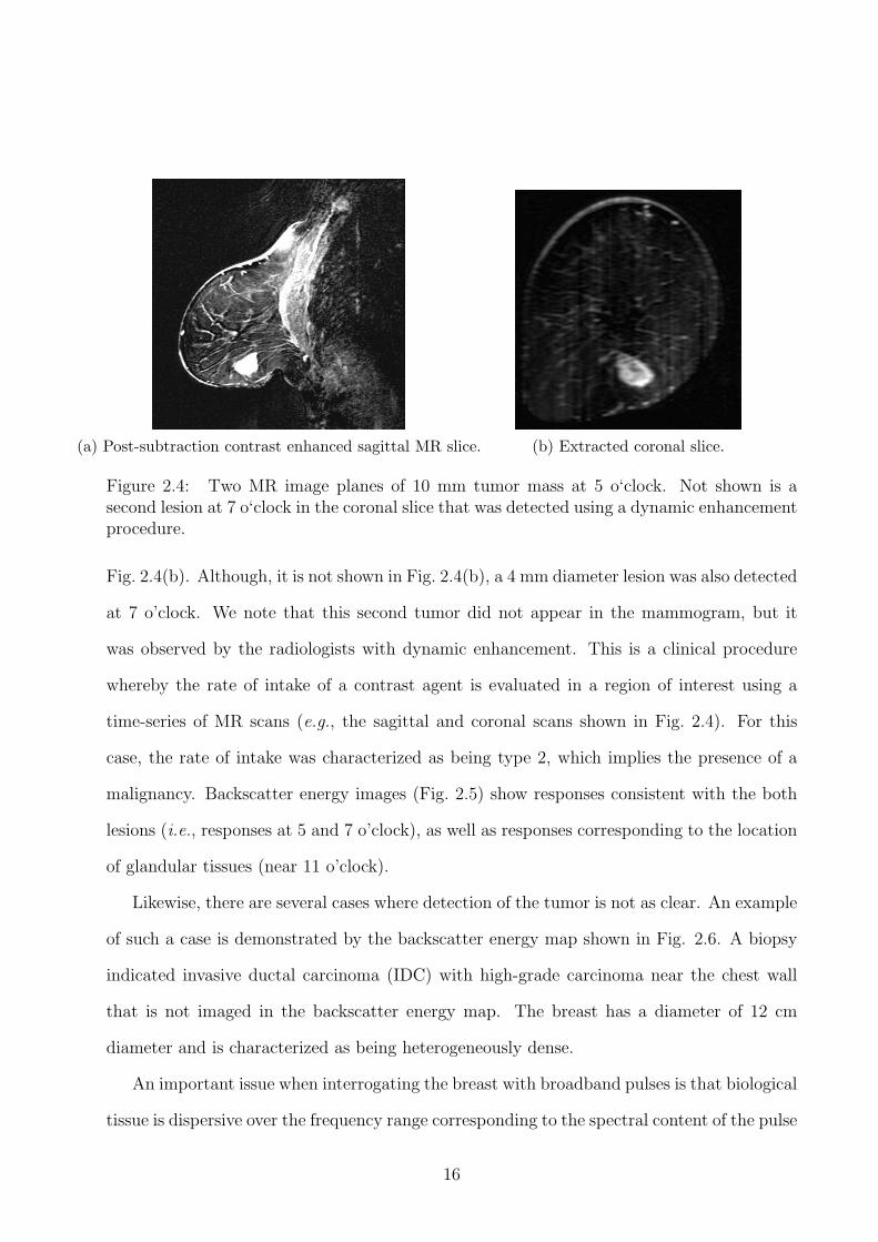
(a) Post-subtraction contrast enhanced sagittal MR slice. (b) Extracted coronal slice.
Figure 2.4: Two MR image planes of 10 mm tumor mass at 5 o‘clock. Not shown is asecond lesion at 7 o‘clock in the coronal slice that was detected using a dynamic enhancementprocedure.
Fig. 2.4(b). Although, it is not shown in Fig. 2.4(b), a 4 mm diameter lesion was also detected
at 7 o’clock. We note that this second tumor did not appear in the mammogram, but it
was observed by the radiologists with dynamic enhancement. This is a clinical procedure
whereby the rate of intake of a contrast agent is evaluated in a region of interest using a
time-series of MR scans (e.g., the sagittal and coronal scans shown in Fig. 2.4). For this
case, the rate of intake was characterized as being type 2, which implies the presence of a
malignancy. Backscatter energy images (Fig. 2.5) show responses consistent with the both
lesions (i.e., responses at 5 and 7 o’clock), as well as responses corresponding to the location
of glandular tissues (near 11 o’clock).
Likewise, there are several cases where detection of the tumor is not as clear. An example
of such a case is demonstrated by the backscatter energy map shown in Fig. 2.6. A biopsy
indicated invasive ductal carcinoma (IDC) with high-grade carcinoma near the chest wall
that is not imaged in the backscatter energy map. The breast has a diameter of 12 cm
diameter and is characterized as being heterogeneously dense.
An important issue when interrogating the breast with broadband pulses is that biological
tissue is dispersive over the frequency range corresponding to the spectral content of the pulse
16

100704R
Axial: y = 51.86 mm
Patient’s right <−−−− x (mm) −−−−> Patient’s left
Che
st <
−−
−−
z
(m
m)
−
−−
−>
Nip
ple
406080100120
10
20
30
40
50
60
Patient’s right <−−−− x (mm) −−−−> Patient’s left
Toe
<−
−−
−
y (
mm
)
−−
−−
> H
ead
Coronal: z = 61.21 mm
406080100120
20
30
40
50
60
70
80
90
100
110
Sagittal: x = 51.48 mm
Nipple <−−−− z (mm) −−−−> Chest
Toe
<−
−−
−
y (
mm
)
−−
−−
> H
ead
20 40 60
20
30
40
50
60
70
80
90
100
110
0
0.5
1
1.5
2
x 1019
Figure 2.5: Backscatter images showing responses (i.e., locations where the backscatter energy is
significant) consistent with lesions located at 5 and 7 o‘clock, as well as responses corresponding to
location of glandular tissues (near 11 o‘clock). Mammography failed to detect the lesion located at
7 o‘clock which was sensed using a dynamic enhancement procedure with MRI.
[12]. These dispersive effects in the signal propagation can introduce noticeable broadening
in the pulse duration (refer to the distorted pulse in Fig. 1.2(a)). An approach based on
broadband beamforming implementing frequency-dependent amplitudes and phase changes
in the various channels has been presented [37]. Since the beamformer design is broadband, it
has the added feature of compensating for the frequency dependent propagation effects [31].
Each received signal is transformed to the frequency domain [37] and passed through a bank
of frequency domain finite impulse response (FIR) filters. The filter coefficients model the
propagation from the antenna to the scatterer and back. The model incorporates the tissue
dispersion as well as a model of the backscatter. Hence, the filters serve to compensate for
frequency-dependent propagation effects by implementing amplitude and phase adjustments
to each signal. The beamformer output is then transformed back to the time domain.
The significant challenge encountered using confocal imaging is that knowledge of the
propagation velocity within the breast is needed to accurately calculate the time delays in
17

100806L
Axial: y = 78.49 mm
Patient’s right <−−−− x (mm) −−−−> Patient’s left
Che
st <
−−
−−
z
(m
m)
−
−−
−>
Nip
ple
20406080100120140
40
60
80
100
Patient’s right <−−−− x (mm) −−−−> Patient’s left
Toe
<−
−−
−
y (
mm
)
−−
−−
> H
ead
Coronal: z = 56.00 mm
20406080100120140
20
40
60
80
100
120
140
Sagittal: x = 93.34 mm
Nipple <−−−− z (mm) −−−−> Chest
Toe
<−
−−
−
y (
mm
)
−−
−−
> H
ead
40 60 80 100
20
40
60
80
100
120
140
0
2
4
6
8
10
12
14
x 1018
Figure 2.6: The maximum responses in the TSAR images appear as ringing above the nipple.
the first step of the beamforming procedure. However, the tissue properties and the internal
structure of the breast are unknown leading to inaccuracies in the wave velocity estima-
tion. This, in turn, leads to uncertainty in the time delay estimates. The uncertainties of
these estimates lead to the deterioration in the performance of the beamformer. This is
demonstrated by the backscatter energy map shown in Fig. 2.6 of a 12 cm diameter breast
characterized as being heterogeneously dense. Although, the breast is heterogeneous, the
TSAR beamforming algorithm assumes that the breast is homogeneous. General a priori
information can be used, e.g., a reasonable estimate of the velocity based on average liter-
ature values [12]. Furthermore, algorithms for estimating the average frequency-dependent
dielectric properties of the breast’s interior have been reported in [38] and [39] to help remedy
this problem. However, these approaches only estimate the average interior properties and
do not take into account the interior structure of the breast specific to the patient.
18

Figure 2.7: A known incident field Einc from transmitter Tx illuminates an object S embedded
in an homogeneous immersion medium Ω. Receivers located on the boundary ∂Ω at r measure the
scattered fields Escat. The aim of microwave tomography is to reconstruct the dielectric properties
ǫ(q), σ(q) of S from the measurements.
2.2 Imaging using transmission/reflection data
Rather than identifying locations of increased scattering due to the presence of a region with
a different permittivity, microwave tomography attempts to recover the spatial distribution
of a target’s electromagnetic properties. Information about the properties is extracted from
the scattered field measured outside the scatterer and the spatial distribution of the electro-
magnetic properties is recovered by solving an inverse scattering problem. The starting point
for the development of these reconstruction methods is a description of the electromagnetic
inverse scattering problem. The description offered is in the context of medical imaging (e.g.,
breast imaging), so microwave near-field approaches are assumed.
Consider the configuration shown in Fig. 2.7 in which an object occupying space S char-
19

acterized by its dielectric properties is embedded in an homogeneous immersion medium Ω
characterized by ǫb and σb which are known. The object is assumed to be penetrable (i.e.,
it has finite electric conductivity) and is nonmagnetic so that µ = µ0. Since the object is
inhomogeneous, its dielectric properties (permittivity ǫ(q ∈ S) and conductivity σ(q ∈ S))
are in general dependent on q where q is a position vector in S (i.e., they are functions of q).
A wave produced by a transmitter located on the boundary ∂Ω at r interacts with the object
and the field distribution is affected by its presence. The field generated by the transmitter
is referred to as the incident (or unperturbed) field, Einc, and is the field in the absence of
the object. It is typically known and can be computed everywhere. The total (or perturbed)
field, E, is the field when the object is present and the difference between the perturbed and
unperturbed fields is referred to as the scattered field. The scattered field is simply,
Escat(r) = E(r) − Einc(r), (2.1)
and arises due to the presence of the object and to the interaction between the incident field
and the object.
In the context of microwave tomography, two scenarios arise. First, given S with a known
dielectric property distribution, the problem is to compute the fields at the receivers when the
object is illuminated by an incident field. We refer to this as the forward problem. Conversely,
when the object is unknown, the problem is to deduce (or reconstruct) its dielectric property
distribution from measurements (i.e., measured scattered fields) collected at discrete receiver
locations. This is referred to as the inverse scattering problem. Microwave tomography
typically considers both problems to achieve the goal of recovering functions ǫ(q) and σ(q).
The electric fields computed by solving the forward problem are compared to the measured
fields at the receiver sites, and nonlinear reconstruction procedures are applied to solve
the inverse scattering problem to obtain a change in the dielectric property distribution in
order to reduce the discrepancy between the measured and computed data. This process is
repeated until convergence (or match) between the measured and computed data is obtained.
20

Volume integral equations offer a physical picture of the mechanisms that give rise to
scattering shown in Fig. 2.7 where the target object is a bound inhomogeneous medium
with support S. The scattered field given by (2.1) is related to the target via a volume
integral equation as follows [21]:
Escat(r) =
∫
S
G(r, q, ǫb)[k2(q) − k2
b ]E(q)dq r ∈ Ω, q ∈ S. (2.2)
where k2b = ω2µbǫb is the wave number squared of the background (or measurement medium);
k2(q) = ω2µ(q)ǫ(q) is the wave number squared of S and it is the function to be sought that
is dependent on position; and ω is the angular frequency in (rad/s) and is related to the
frequency f in Hertz by ω = 2πf . The dyadic Green’s function of the background profile,
G(r, q, ǫb), is the solution of the equation [21],
××G(r, q, ǫb) − k2b G(r, q, ǫb) = Iδ(r − q), (2.3)
where I is the identity matrix, and δ is the Dirac delta function. The scattered field results
from the re-radiation of the total field in S that arises from the dielectric contrast formed
by the difference between the object profile, ǫ(q), and the background dielectric ǫb. The
scattering contribution measured at r due to the dielectric contrast at q ∈ S is determined
by the Green’s function of the background dielectric profile. In other words, in the context of
the inverse scattering problem, this dyadic function is the kernel of the volume integral and
relates fields in the target domain to observed scattered fields outside the target domain.
The contrast function, χ(q), is defined as,
χ(q) = ω2(µǫ− µbǫb) = k2(q) − k2b , (2.4)
and is substituted into (2.2) which simplifies to,
Escat(r) =
∫
S
G(r, q, ǫb)χ(q)E(q)dq r ∈ Ω. (2.5)
This integral is expressed compactly in operator form with,
Escat(r) = LΩ(χE) r ∈ Ω, (2.6)
21

where LΩ is the integral operator (or data operator) in (2.5) given by,
LΩ(ψ) =
∫
S
G(r, q, ǫb)ψ(q)dq r ∈ Ω. (2.7)
Equation (2.6) relates the continuous spatial dielectric property distribution within S to the
scattered field measured at points outside of S in Ω. It provides the key relationships nec-
essary to establish the basic framework for a general inverse scattering problem formulation
and is referred to as the data equation. We note that the electric field is a functional since
it is a function of the dielectric properties which themselves are functions of space. Further-
more, if the output is sampled at a finite number of points and the integral is discretized
(e.g., using the quadrature approach [40]), then the data equation may be expressed with a
set of linear discrete equations.
There are two sets of unknowns, namely the electric field inside S and the dielectric
property distribution of the target. The general approach used by the tomography methods
to search for the unknown dielectric property distribution of the target is by recasting the
inverse scattering problem to the minimization of a suitable cost functional. We note that
the total field E is unknown within S and is a function of χ, making the system nonlinear in
the unknown contrast function. To handle the nonlinearity of the functional, the tomography
methods implement an iterative scheme based on successive linearization of the nonlinear
problem. In the context of an optimization problem, one of two cost functionals is formulated.
Most tomography approaches formulate a cost functional based only on the scattered fields
outside the target. The distorted Born iterative method (DBIM) is representative of this class
of methods and is reviewed in Section 2.2.1. The contrast source inversion method (CSIM)
reviewed in Section 2.2.2 provides an alternative formulation based on both the scattered
fields outside the target and the total fields inside the target. Since this thesis uses a broad-
band approach to tomography, time-domain techniques are described in Section 2.2.3. Like
the DBIM approach, the time-domain techniques recast the inverse scattering problem to
the minimization of a cost functional based only on the scattered fields outside the target.
22
Finally, in addition to extracting dielectric property information about an object, this thesis
also presents a technique to extract information corresponding to boundaries (or interfaces)
that segregate regions of different dielectric properties within an object. Therefore, state-of-
the art shape localization and support methods are reviewed in Section 2.2.4.
2.2.1 Distorted Born Iterative Method (DBIM)
The DBIM is distinguished from the CSIM method in that its formulation is based only
on the scattered fields outside the target. For an inverse scattering problem, field data are
measured outside the scatterer S on surface ∂Ω as shown in Fig. 2.7. In sequence, each
antenna in the array transmits an incident field, Eincm , of one single frequency into S while
the other antennas act as receivers and measure the corresponding scattered field. That is,
we assume that for each set of field measurements, numbered from m = 1, 2, . . . Tx, the target
is illuminated successively by an incident field. Therefore, we have (2.2) at our disposal to
evaluate the scattered field.
Due to the relationship between the object dimensions, discontinuity, separation, and
contrast in properties of inhomogeneities compared to the wavelength, the incident wave un-
dergoes multiple scattering within the object to be reconstructed. This results in a nonlinear
relationship between the measured scattered fields and the object’s contrast function [21].
However, under certain circumstances, an approximate solution is possible by expressing the
scattered field as a linear functional of the target. This formulation is commonly referred to
as the Born approximation and can be implemented whenever the scatterer to be inspected
is weak with respect to the propagation medium (i.e., discontinuities in the dielectric profile
are small so that k2(q)−k2b is small). This implies that the scattered field is small compared
to the incident field so that the expression given by (2.1) simplifies to the approximation,
Einc(q) ≈ E(q). (2.8)
Since Einc(q) is known, the scattered field given by (2.6) may now be expressed with the
23

linear approximation,
Escat(r) ≈ LΩ(χEinc). (2.9)
Guidelines are provided in [41] that describe the conditions for which (2.9) is valid (i.e., a
weak scatterer is defined). Equations of this kind are known as linear Fredholm integral equa-
tions of the first kind [42]. We note that the data operator, LΩ, is a compact linear operator
on L2(Ω) [43]. According to the Riemann-Lebesgue lemma [42] [44], the physical interpreta-
tion of this property is that the integration of the kernel G in (2.9) has a “smoothing” effect
on χEinc in that high-frequency components, cusps, and edges in χEinc are “smoothed out”
by the integration. Likewise, the reverse process, i.e., computing χEinc from the scattered
field, will tend to amplify any high-frequency components in χEinc (e.g., discontinuities in
the profile and noise) [42]. The generalized inverse operator required to compute the ap-
proximation for χEinc from the scattered field may be unbounded [45]. Mathematically, this
is an ill-posed problem [43] when this is the case since the inverse solution does not depend
continuously on the data. This means that the inverse solution is unstable since even a
small random perturbation of the scattered field can lead to a very large perturbation of
the reconstructed profile. To remedy the problem, the inverse operator must be replaced
by bounded approximations so that numerically stable solutions can be defined and used as
meaningful approximations of the true solution corresponding to the exact data. This is the
goal of regularization, and techniques used to restore stability are examined in Chapter 3.
Unfortunately, the linearized approach has very limited utility in the context of medical
imaging due to the high contrast in tissue dielectric properties. That is, linearized inverse
problems make significant assumptions regarding the wave propagation within the scatterer
and, when applied to practical problems, do not offer enough accuracy to provide useful
quantitative imaging. Two image reconstruction algorithms for microwave tomography (one
linear and the other is nonlinear) are compared and contrasted in [46]. The study provides
important insight into the limitations of linear approaches. Nevertheless, a linear approxi-
24

mation may be embodied into an iterative procedure that may be used to find approximate
solutions in high contrast scenarios. The iterative scheme is referred to as the distorted Born
iterative method (DBIM) [22] and is based on repeatedly linearizing the nonlinear problem
around the solution from the previous iteration. This is repeated for a number of iterations
until an approximate solution is reached.
The relation in (2.6) is linearized using the Born approximation whereby the unknown
total field E(q ∈ S) in S is approximated by the incident field Einc(q ∈ S). The incident
field in the presence of the background medium, ǫb, is referred to as the background field,
Eb(q ∈ S). In the context of the Born approximation, this means that the field, Eb(q),
within the background profile replaces the unknown total field, E(q), in (2.6). Therefore, for
the ith iteration, the Born approximation in (2.9) is written as,
Escat,i(r) ≈ LiΩ(δχiEb,i). (2.10)
where δχi is the relative change in the contrast function. The data operator is given by,
LiΩ(ψ) =
∫
S
Gi(r, q, ǫb)ψ(q)dq r ∈ Ω. (2.11)
where Gi is the Green’s function of the background dielectric profile for the ith iteration and
must be updated with each iteration since the background profile is also updated (or refined
with each iteration). The method iteratively refines the contrast function beginning with
an initial guess of the background profile. For the given background profile, the forward
solution is computed to evaluate the fields inside S, the fields at the antennas, and the
Green’s function, Gi. The contrast function is updated with, δχi, obtained by solving the
minimization problem that is formed from a system of scattering equations constructed from
the forward solution and the measurement data and is given by:
δχi = arg minχ
Tx∑
m=1
‖Emeasm − Escat
m − LiΩ(δχiEb,i
m )‖22, (2.12)
where Emeasm and Escat
m are the measured and calculated scattered fields, respectively. The
25

inverse solution is obtained by solving the normal form of (2.12), namely
(LiΩ)∗ Li
Ω (δχiEb,im ) = (Li
Ω)∗ ∆i (2.13)
where (LiΩ)∗ is the adjoint operator, and ∆i
m = Emeasm − Escat
m (χi) is the discrepancy be-
tween the measured and calculated fields. Finding the inverse solution using (2.13) typically
requires regularization to replace the inverse operator by bounded approximations so that
numerically stable solutions can be defined and is discussed in Chapter 3. The contrast
function is updated with the inverse solution using,
χi+1 = χi + δχi. (2.14)
The updated estimate, χi+1, is used to calculate the background profile using (2.4). For the
given updated background profile, the forward solution is re-computed to evaluate the fields
inside S, the fields at the antennas, and the Green’s function. The minimization problem
given by (2.12) is solved with the updated scattering equations to obtain an inverse solution
that is used to update the contrast function. The DBIM algorithm continues in this manner
by alternating between the forward and inverse solutions and updating the background
profile at each iteration. The DBIM algorithm is terminated once the background profile
found produces calculated data that closely matches the measurement data (i.e., residual
scattering sufficiently converges).
It is important to note that the Gauss-Newton iterative method (GNIM) is equivalent to
the DBIM [47]. Like the DBIM method, the GNIM is based on a formulation of the scattered
field outside the target and is given by,
χ = arg minχ
Tx∑
m=1
‖Emeasm − Escat
m (χ)‖2Ω. (2.15)
which is a nonlinear optimization problem since the unknown distribution, χ, is embedded
in the functional for the calculated fields, Escat (cf [48] or [49] for more details). An iterative
scheme based on successive linearization of the nonlinear problem is used to find an approx-
imate solution. The nonlinear expression for the scattered field as a function of the contrast
26

distribution is repeatedly approximated locally by a first-order Taylor expansion as,
Escat(χi + δχi) ≈ Escat(χi) + J iδχi (2.16)
where J i is the Jacobian matrix containing the Frechet derivatives of Escat with respect
to χ evaluated at χi; δχi = χi+1 − χi; and i is the current iteration number. The linear
approximation of Escat using the Taylor expansion method forms the linear optimization
problem,
δχi = arg minδχ
Tx∑
m=1
‖∆im − J iδχi‖2
Ω, (2.17)
where ∆im = Emeas
m −Escatm (χi) is the discrepancy between the measured and calculated fields.
The minimization of (2.17) is solved with the Gauss-Newton method expressed as,
J iH J i δχi = J iH ∆i, (2.18)
where (·)H is the Hermitian transpose. As pointed out in [47], the equivalence between the
DBIM and the GNIM is derived from the fact that the Jacobian matrix, J i, operating on
the update, δχi, is the same as,
J i δχi = LiΩ(δχiEi
m). (2.19)
Therefore, by replacing J i δχi with LiΩ(δχiEi
m) in (2.17), we see that the optimization prob-
lems given by (2.17) and (2.12) are equivalent. Due to this equivalence, the DBIM and the
GNIM share a similar approach to regularization (e.g., projection method or cost functional
augmented by penalty term) which are reviewed in Chapter 3. It is noted that GN based
optimization approaches require significantly fewer iterations to converge to the approximate
solution compared to gradient type optimization techniques like the CSIM (cf [50] or [51]).
Needing fewer iterations for convergence lowers the overall computational cost of the algo-
rithm. This aspect was considered by a study [47] that compares the computational cost of
the DBIM with the CSIM algorithm. The study is reviewed in Chapter 3.
Although the GN methods are efficient in terms of convergence speed, multiple executions
of the forward solver is a computational burden and is the chief disadvantage using these
27

methods compared to other approaches. To reduce the computational burden required to
execute the forward solver for 3D scenarios, the volume integral equation in (2.6) can be
discretized and solved numerically based on the discrete dipole approximation (DDA) [52]. It
is observed in [5] that this enhancement leads to a considerable saving in computational time
and memory compared to a numerical approach such as the finite-difference time-domain
technique. Another disadvantage of using the GN type methods is that these methods are
more sensitive to the initial guess than the gradient optimization techniques [53]. As a
remedy, a logarithmic version of (2.15) is used in [54], whereby the amplitude and phase
differences of the electric field are minimized rather than real and imaginary parts.
In the context of breast microwave imaging, examples of the DBIM method applied
to realistic 3D numerical breast models are demonstrated in [55] [27] [56] [57]. For these
examples, z -polarized dipole antennas are used to provide the excitation source. These
simple structures are easy to model so that the forward model can be quickly and efficiently
solved to reduce the computational costs. Moreover, the use of z -directed fields leads to
scalar sourcing and observation of z-directed fields. Hence, scalar field approximations of
the Green’s function tensor are implemented to further reduce the computational costs. For
the reconstructed images shown in these examples, it is observed that there are regions of
fibroglandular tissue that appear smeared and small features of the tissue structure are not
resolved. For this scenario, the limited resolution provided by microwave imaging effectively
results in reconstructions having regions that are spatially averaged [27]. Furthermore, the
abrupt transition between tissue types in the profiles (i.e., interfaces) appear blurred in
the reconstructed images. The regularization technique used to stabilize the solution and to
remedy the problem of non-uniqueness (i.e., address the ill-posedness of the inverse scattering
problem) contributes to this problem and is discussed in greater detail in Section 3.1.1. In
[17], breast tissue is imaged in a clinical setting using the GNIM. Reconstructions with
smeared regions of fibroglandular tissue and blurred interfaces are also observed.
28

2.2.2 Contrast source inversion method (CSIM)
Unlike the distorted Born iterative method, the contrast source inversion method introduced
by Van den Berg and Kleinman in [58] considers fields both internal and external to the
object. For an observation point q inside S, (2.1) is rearranged to obtain the total field inside
S given by,
E(q) = Einc(q) + Escat(q). (2.20)
The total field is related to the target via a volume integral as follows:
E(q) = Einc(q) + LS(δχ(q)E(q)) q ∈ S. (2.21)
The integral operator LS (or object operator) is,
LS(ψ) =
∫
S
G(r, q, ǫb)ψ(q)dq q ∈ S. (2.22)
The relation given by (2.21) may also be expressed in terms of the equivalent contrast source
within S due to a transmitting antenna. Multiplying both sides of (2.21) by χ(q) yields,
χ(q)E(q) = χ(q)Einc(q) + χ(q)LS(χ(q)E(q)), q ∈ S. (2.23)
The scattered field can be considered to be generated by an equivalent electric current density,
so the equivalent contrast source is,
W (q) = χ(q)E(q). (2.24)
These sources have support coinciding with the space occupied by the target [58]. Substi-
tuting (2.24) into (2.23) leads to,
W (q) = χ(q)Einc(q) + χ(q)LS(W (q)), q ∈ S. (2.25)
In this context, the dyadic Green’s function is used to determine the total field solution inside
the target domain. Equation (2.25) is referred to as the object equation since it corresponds
29

to the total field inside the target. Rearranging (2.25), the discretized set of object equations
defined in symbolic form is given by,
χEinc = W − χLSW, q ∈ S. (2.26)
Likewise, the discretized set of data equations (i.e., equations that relate the continuous
spatial dielectric property distribution within S to the scattered field measured at points
outside of S in Ω) given by (2.6), in symbolic form is,
Escat = LΩW, r ∈ Ω. (2.27)
Measurements of the scattered fields Emeas(r ∈ Ω) approximate the scattered field Escat(r ∈
Ω) and are used to find χ(q ∈ S) and E(q ∈ S). As already noted in Section 2.2.1, the data
operator is compact, so the data equation (2.27) is an ill-posed nonlinear integral equation for
the unknowns χ(q ∈ S) and E(q ∈ S). Regularization techniques are discussed in Chapter
3.
Formulated in this way, the data equations tell us that the solution to the inverse problem
requires a search for the object that produces a prescribed scattered field, but at the same
time produces an internal field distribution consistent with the known incident field inside
the object viz. the object equation. Therefore, we can view the presence of the internal
field represented by the object equation (2.26) as a physical constraint imposed by the
requirement to satisfy the data equation (2.27). For this contrast source formulation the
inverse problem is treated in its nonlinear form where the problem unknowns are the contrast
function and the equivalent current density which is directly related to the internal field. To
reconstruct the contrast function, we assume that for each set of measurements, numbered
from m = 1, 2, . . . Tx, the target is illuminated successively by an incident field, Eincm , of
one single frequency. The inverse scattering problem is recast as a constrained optimization
problem given by,
χ = arg minχ
Tx∑
m=1
‖Emeasm − LΩWm‖2
2 (2.28)
30

subject to,
χEincm = Wm − χLSWm, q ∈ S. (2.29)
This minimization forms the basis of the formulation of a cost functional expressed in terms
of the contrast sources and contrast function and is used to generate sequences Wm,i and
χi for iterations i = 1, 2, . . . which are found by minimizing,
Fi(Wm,i, χi) =Tx∑
m=1
ηΩ‖Emeasm − LΩWm,i‖2
Ω + ηS‖χiEincm −Wm,i + χiLSWm,i‖2
S (2.30)
where ‖‖2Ω denotes the ℓ2-norm on Ω; ‖‖2
S denotes the ℓ2-norm on S ; ηΩ = (∑
m ‖Emeasm ‖2
Ω)−1
and ηS = (∑
m ‖χi−1Eincm ‖2
S)−1 are normalization terms used to balance between the data and
the object equation, respectively. We note that the object equation normalization changes
with each iteration of the algorithm as the contrast function is updated. The first term of
the cost functional measures the error in the data equation given in (2.27) and the second
term measures the error in the object equation given in (2.26). The cost functional is written
more compactly as,
Fi(Wm,i, χi) = Fdata,i(Wm,i) + Fobject,i(Wm,i, χi). (2.31)
The contrast source formulation uses a two stage approach to minimize (2.31) in order to
to recover a sequence of estimates of the contrast function χi and the contrast source W i
(cf [59] [60]). In the first stage, the contrast source sequence W i is updated via a single
step of the conjugate gradient minimization algorithm of (2.31) while assuming that the
contrast function χi is constant. In the following stage, once W i is evaluated, the contrast
function sequence χi is updated with a single step of the conjugate gradient method to
minimize the cost functional while W i is constant. Continuing in this manner, the CSI
method alternatively constructs sequences of contrast sources W i by a conjugate gradient
iterative method such that the contrast sources minimize the cost functional for an assumed
fixed value of the contrast function from the previous iteration. That is, each sequence is
updated via the a single step of the CG minimization algorithm while assuming that the
31

other unknown is a constant. The iterative process is continued in this manner until a desired
minimum of the cost functional is reached. Details of the CSIM method are in [61].
A key feature that distinguishes the CSIM from other techniques is that the cost func-
tional is based on both the scattered fields outside the target and the total fields inside the
target. This formulation does not require the use of a forward solver at each step of the
minimization process with the inclusion of the additional constraint provided by the target
equation. Hence, this method is computationally efficient compared to methods that execute
multiple calls to the forward solver at each iteration. However, although the forward solver
is not executed at each iteration, multiple calls are made to the data operators (LΩ) and the
target operators (LS). Moreover, the CSIM is referred to as a first order optimization tech-
nique since it only uses gradient information to evaluate the direction of parameter change.
Gradient type optimization techniques typically require more iterations to converge to the
approximate solution than Gauss-Newton (GN) type optimization approaches [53]. A de-
tailed evaluation of the computational resources used by the CSIM and DBIM methods are
reported in [47] and are reviewed in Chapter 3. Another key difference between the DBIM
and the GN type methods is that the CSIM may be formulated so that the regularization is
completely automatic. This is also discussed in more detail in Chapter 3.
An excised segment of a pig hind-leg is imaged using a 3D microwave-tomography system
based on the CSIM and operating at frequencies of 0.9 and 2.05 GHz in [10]. This application
uses rectangular waveguides for the transmitters and receivers (which are linearly polarized
in the z-direction) and models these devices with a unit vertical electric dipole. The approx-
imation is very appealing since it simplifies the formulation of the Green’s function. The
technique is applied to a range of biomedical applications including thorax imaging, brain
imaging, and breast imaging in [62]. For these examples, the algorithm is applied to numer-
ical 2D data and line sources are used for antennas. Also in [47], the algorithm is applied to
experimental data. Specifically, a forearm is imaged along with plastic cylinders.
32

2.2.3 Conjugate Gradient Time-domain technique
Up to this point, only frequency domain microwave tomography methods have been de-
scribed. Low profile dipoles as described in [5] are commonly used when implementing these
techniques. Consequently, for the DBMI and the GN methods, these sensors are simple to
model and can be efficiently and accurately incorporated into the forward solver. Likewise,
using these simple structures also ensures that the Green’s function in (2.5) can be easily
approximated as described in [27]. For the CSIM formulation, the simple antenna structures
allows accurate and efficient formulation of the data operators (LΩ) and the object operators
(LS).
A disadvantage of using the frequency-domain approach is the stability-resolution trade-
off. That is, increasing the frequency of the illuminating field leads to the obvious possibility
to resolve finer structures. Unfortunately, this approach results in complications when imag-
ing large structures and high contrast objects since the scattered field is nonlinearly related
to the scattering object. The nonlinear dependence is due to the mutual interactions between
the induced electric displacement currents and multiple scattering interactions between fea-
tures of the dielectric profile [21]. As expected, the nonlinearity is more pronounced at high
frequencies [63] (i.e., the size of the object relative to the wavelength increases). Therefore, as
the body becomes large compared to the wavelength or when contrasts of the inhomogeneity
become large, the nonlinear effect (or multiple scattering effect) becomes more pronounced.
A stability-resolution trade-off appears to occur when choosing an appropriate frequency
for the illuminating field of a monochromatic source. On the one hand, the use of mono-
frequency data at a high frequency often results in the inverse algorithm being trapped in
local minima due to the highly nonlinear nature of the problem; on the other, reconstructed
images appear smoother and with less detail when the reconstruction algorithm is utilizing
single operating frequencies with lower frequency. However, the lower frequency reconstruc-
tions also exhibit more stable convergence behavior to a viable solution compared with the
33

less stable higher frequency cases [63].
When imaging complex objects for medical applications, it is important that the imaging
algorithm be able to reconstruct both the overall structure of the object and resolve the
small objects inside the large structure. To meet this requirement, multi-frequency data
are collected over discrete frequencies using a stepped frequency measurement approach as
described in [64]. The data are then incorporated into the reconstruction algorithm using a
multiple frequency approach. The basic idea of the multiple frequency approach is that the
low frequency measurement data have a stabilizing effect on the reconstruction algorithm,
whereas higher frequency data is included to reconstruct images with improved resolution.
Typically, the data from several frequencies are used simultaneously to obtain a solution.
For example, a multiple frequency dispersion reconstruction algorithm utilizing the GNIM
and the DBIM is presented in [65] and [55], respectively.
As indicated in Chapter 1, it is important that the radar-based system used to extract an
object’s internal structural information be easily integrated with the microwave tomography
system used to image the dielectric profile of the object. To ease this integration, a require-
ment is for the two systems to share the same components. For example, the microwave
tomography system will share the well-designed UWB sensors [66] with the radar-based sys-
tem. It also makes practical sense to be able to leverage the expertise and knowledge put
into the radar-based measurement system [36] [18] to microwave tomography. The use of
the UWB sensors leads to the concept of broadband, or time-domain, microwave tomogra-
phy. For this variant of microwave tomography, the image reconstruction is conducted using
a time-domain algorithm where the pulses are synthesized from frequency domain data.
Therefore, instead of using only a few frequencies, an entire frequency range is used.
Time-domain microwave tomography methods have been developed and examples are
described in [67] and [68]. These methods are based on the cost functional given by
F(ǫ, σ) =
∫ T
0
M∑
m=1
N∑
n=1
(|Ecal,m(ǫ, σ, rn, t) − Emeas,m(rn, t)|2
)dt (2.32)
34

where Ecal,m(ǫ, σ, rn, t) is the calculated field from the computational model; Emeas,m(rn, t)
is the corresponding measured data with antenna number m used as a transmitter and
antenna n as the receiver; M is the number of transmitters; N is the number of receivers;
t is the time variable; and T is the duration of the pulse. The gradients of type ∂F/∂ǫ
and ∂F/∂σ in each reconstruction element of the reconstruction model are evaluated using
the adjoint method. The adjoint method evaluates closed form expressions of the gradients
formed from a forward Finite-Difference Time-Domain (FDTD) computation followed by
a corresponding adjoint FDTD computation in which residual received signals denoted as
Ecal,m(ǫ, σ, rn, t) − Emeas,m(rn, t) are used as equivalent sources which are reversed in time
[67].
The underlying idea of the CG method is to update the current solution with
ǫn+1 = ǫn + αndǫn, (2.33)
σn+1 = σn + αndσn, (2.34)
where αn is a scalar corresponding to the step length; dǫn and dσ
n is the conjugate search
direction for the change in ǫ and σ, respectively. The conjugate search direction for the
parameter change is calculated from the gradients. The step length is determined optimally
with
αn = arg minα
F(ǫn + αndǫn, σn + αnd
σn). (2.35)
A line search is then used to solve the nonlinear 1D optimization problem in (2.35) to
approximate the step length of the parameter change. A successive parabolic interpolation
line search is used by [69] to evaluate αn. Computationally, this is described in [69] as the
most intensive part of the reconstruction algorithm since each evaluation of the objective
functional requires an FDTD computation of the forward problem. It is noted in [68] that
typically, about 5-10 complete simulations are required to find the minimum of the line
search.
35

The dielectric properties of 3D numerical breast phantoms are reconstructed as part of
an investigation described in [70]. For this investigation, full knowledge of skin location,
thickness, and properties are assumed. Furthermore, point sources are used instead of UWB
antennas. This approach is convenient for initial feasibility studies since antenna models
are not incorporated into the forward model. The reconstruction models do not incorporate
dispersive properties and a significant contrast between tumor and surrounding breast tissue
is used.
Numerical and experimental studies using plastic cylinders in saline and tap water so-
lutions are investigated in [69]. A pseudo 3D reconstruction technique is used whereby
constant properties of the test object as a function of height are assumed. Importantly,
for this implementation, monopole antennas are used. Therefore, like the frequency domain
approaches, these structures can be accurately and efficiently incorporated into the forward
solver. Furthermore, the solution of the inverse problem relies on the comparison between
the measured and calculated scattering data. In a practical scenario, it is not possible to
create an antenna model without modeling errors that contribute to discrepancies between
the measured and the simulated data. A calibration procedure for the measured data to
account for this discrepancy is required and is described in [69] and [71]. The calibration
procedure is much easier for a monopole antenna than for a more complicated UWB sensor.
These time-domain microwave tomography methods estimate a very large number of pa-
rameters and solve very large scale problems. Solving a time-domain microwave tomography
problem using this approach is not practical with the UWB sensors and so alternative ap-
proaches are required. This is the motivation for the development of an efficient inverse
solver and one of the core problems that this thesis seeks to solve.
2.2.4 Object support and shape determination algorithms
In this thesis, methods to extract internal structural information from objects are investi-
gated. These methods are described in Chapters 4, 5 and 7 and evaluate points on interfaces
36

segregating regions. Other methods are described in literature that may be applied to local-
ize an unknown scatterer and define its shape. More specifically, the goal of these methods
is to retrieve the support of the target in order to reconstruct its shape from the measure-
ments of scattered fields. The linear sampling method (LSM) and the level-set method are
reviewed.
Linear sampling method (LSM)
The linear sampling method (LSM) is a non-iterative method introduced by Colton and
Kirsch and is described in [72]. This method evaluates the support of the scatterer in a
direct and fast manner. An extension of the LSM is presented in [15] and is used to find
scatterers with respect to an unperturbed background. The key assumption used by this
extension is that the Green’s function of the inhomogeneous background is known. The
algorithm is used in [15] [16] for detecting the presence of leukemia in a human leg. For
this scenario, the heterogeneous background tissue is known in order to compute the Green’s
function and the diseased tissue is assumed to be homogeneous with known properties. A
further extension of the method is also proposed in [73] as a tool to detect cancerous tissues
inside the female breast. For this extension, the underlying tissue structure and dielectric
property distribution are assumed known and are available using an MRI scan in order to
construct the corresponding reference background Green’s function. This example represents
an intriguing multi-modality approach for breast screening whereby the LSM is presented
as a microwave imaging technique to be used to complement other imaging modalities. It
is discussed further in Chapter 3. In the context of medical applications, the LSM method
and its variants are appealing because of the speed and efficiency for which the support of
the scatterer is evaluated. The disadvantage using these methods is the requirement for a
priori knowledge of the underlying structure in which the scatterer is embedded.
37

Level-set method
Structural information may also be acquired at microwave frequencies using level-set ap-
proaches. This tomographic method approximates the location of interfaces between regions
by solving an inverse scattering problem. The interfaces between regions are represented by
level set curves; one level set is used for each interface. The method assumes homogeneous
material within the region bounded by each curve. An iterative procedure uses the non-
linear cost function similar to (2.15) to approximate interface locations and the dielectric
properties of the homogeneous material within the contours. Like the microwave tomogra-
phy techniques discussed in Sections 2.2.1 and 2.2.2, this method solves a highly nonlinear,
ill-posed inverse scattering problem. Furthermore, similar to the DBIM, the forward problem
is solved multiple times at each iteration of the algorithm.
The feasibility of the technique to detect unknown anomalies (e.g., cracks) in dielectric
materials is evaluated in [2]. The application of shape-optimization techniques to numer-
ical and experimental data for microwave imaging of perfect electric conductor objects is
presented in [74] and [75], respectively. A similar approach is also proposed for microwave
breast imaging (see [76] or [77] for examples). Unlike the LSM method which finds the
support of the scatterer in a fast and efficient manner, this shape-optimization approach
faces significant computational and mathematical challenges since the objective functional is
nonlinear (i.e., it has multiple solutions), the problem is severely ill-posed, and the contour
information is extracted from the transmission data using only a few frequencies. Additive
penalty regularization, as discussed in Chapter 3, is used to stabilize the solution. For many
medical applications, the object of interest (e.g., a breast) is a heterogeneous organ with a
complex anatomical structure. The complex nature of the internal structure of the object for
these applications, the lack of prior information about the internal structure, and limitations
in the quality and quantity of the measurement data lead to a multitude of challenges when
implementing the level-set approach.
38

2.2.5 Discussion and concluding remarks
In this chapter background information pertaining to medical microwave imaging has been
presented. In particular, the leading methods that are currently being investigated have
been described. The goal of radar-based microwave imaging algorithms is to identify the
location of scatterers, namely locations where there is an abrupt dielectric property contrast
(or discontinuity) such as an interface. The microwave tomography methods have a more
ambitious goal by attempting to provide complete information about the spatial distribu-
tion of an object’s electromagnetic properties. There are a variety of microwave tomography
methods that may be used for this task. Most are frequency-domain microwave tomography
methods and are distinguished from each other by the formulation of the cost function used
to find the unknown contrast function. The formulation of the DBIM and GNIM is based
only on scattered fields outside the target whereas the formulation of the CSIM is based on
the fields both outside and inside the target. This thesis investigates the development of a
time-domain microwave tomography method. The use of time-domain microwave tomogra-
phy is motivated by the need to easily integrate tomography with the radar-based system
for which it extracts structural information about the object. A conjugate-gradient time-
domain microwave tomography was reviewed. Similar to the frequency-domain microwave
tomography methods, the aim of this technique is to provide a detailed reconstruction of the
target’s dielectric profile.
Object support and shape determination algorithms were also reviewed. The LSM is
fast and efficient, however, it requires prior knowledge of the underlying structure in which
the scatterer is embedded. Unlike the LSM method which finds the support of the scatterer
in a fast and efficient manner, the level-set method faces significant computational and
mathematical challenges since the objective functional is nonlinear (i.e., it has multiple
solutions), and the problem is severely ill-posed.
The microwave tomography methods all face the same challenge by attempting to solve
39

an inverse scattering problem that is nonlinear and highly ill-posed. Iterative approaches are
used to address the nonlinearity challenge and there are a wide variety of approaches that
are employed to mitigate the non-uniqueness and instability difficulties that arise due to the
ill-posed nature of these problems. These methods are discussed in Chapter 3.
40

Chapter 3
Regularization techniques
As indicated in Chapter 1, a significant difficulty when solving microwave inverse scattering
problems is that they are severely ill-posed. This problem is viewed by many as the most
crucial impediment preventing the successful implementation of this imaging technique, es-
pecially for high contrast scenarios such as medical applications. Mathematical techniques,
known as regularization, have been developed to help mitigate this problem. These tech-
niques replace the original ill-posed problem with another well-posed problem, in which some
additional information is added. The approach used is dictated primarily by the type and
quality of prior information that is available. In the context of breast imaging with mi-
crowave tomography, the prior information ranges from none (i.e., blind inversion) to high
resolution object-specific information such as MR scans. The prior information has two
challenges associated with it: (1) acquiring high quality object-specific information, and (2)
once the information is acquired, integrating this knowledge into microwave tomography.
Addressing these challenges is the core problem that this thesis attempts to solve.
Before examining state-of-the art regularization tools, the motivation for using these
techniques is reviewed. As an example, recall in Chapter 2 that the DBIM iteratively recon-
structed the dielectric property profile by updating the contrast function with, δχi, obtained
by solving the minimization problem given by:
δχi = arg minχ
Tx∑
m=1
‖∆im − Li
Ω(δχiEb,im )‖2
2, (3.1)
where ∆im = Emeas
m −Escatm (χi) is the discrepancy between the measured and calculated fields.
The minimization of (3.1) is solved with the normal form of (3.1), namely
(LiΩ)∗ Li
Ω (δχiEb,im ) = (Li
Ω)∗ ∆im. (3.2)
41

An inverse problem such as the one given by (3.2) is well-posed provided three requirements
are fulfilled [78]: (1) the solution exists for any data, (2) the solution is unique, and (3) the
solution depends continuously on the data. The problem is said to be ill-posed if any one of
these conditions is not met [79].
For microwave tomography the existence criterion is typically satisfied. As long as a
reasonable amount of sufficiently accurate measured data are available, a solution exists as
the aim of tomography is to find the internal properties of an existing object of interest.
A fundamental challenge facing tomography is that the number of reconstruction elements
(i.e., the dimension of the solution space) far exceeds the number of independent data. For
the nonlinear inverse scattering problem, after the cost function is linearized, this typically
leads to underdetermined systems of equations, i.e., systems of linear equations with fewer
equations than unknowns. This is the so-called “large p, small n paradox” or overcomplete-
ness problem [80] and we are left to conclude that there are infinitely many solutions since
we have a system of linear equations with fewer equations than unknowns. Therefore, in
order to obtain a unique inverse solution, we need additional prior information on the un-
known object. Not satisfying the third condition also presents a severe challenge for inverse
problems. As shown in Chapter 2, the data operator LΩ given by (2.7) that relates the
continuous spatial dielectric property distribution within S to the scattered field is a linear
compact operator on L2(Ω) [43]. From (3.2), we see that obtaining the inverse solution makes
use of the inverse of the operator (LiΩ)∗ Li
Ω. This operator is bounded when its spectrum is
bounded below and away from 0 [81]. Conversely, when its spectrum is not bounded below
by a strictly positive constant, then ((LiΩ)∗ Li
Ω)−1 is unbounded and severe numerical insta-
bility may occur when attempting to obtain an inverse solution [81]. Mathematically, this
is an ill-posed problem [43] since the inverse solution may not depend continuously on the
data. The inverse solution is unstable since a small random perturbation of the scattered
field can lead to a very large perturbation of the reconstructed profile. The occurrence of
42

this numerical instability is regarded as “unphysical” in that we typically know beforehand
that the actual profile would not have a large norm or other characteristics exhibited by the
unconstrained inverse solutions. Whether a problem is well-posed or ill-posed is determined,
in practice, by the operator LΩ (or more specifically, the kernel G) [82] [42]. However, in
theory, this is also determined by the solution and the data spaces, including the norms
[82] [42]. Various authors have attempted to quantify the level of ill-posedness of microwave
inverse scattering problems (cf, [23], [24]). In order to solve an ill-posed problem the stability
has to be restored.
The use of regularization techniques allows a stable approximate solution to the ill-posed
problem to be constructed so that the inverse scattering problem is uniquely solvable and the
solution is robust in the sense that small errors in the data do not excessively corrupt this
approximate solution (cf [79] [83] [42]). The regularization method used is dictated primarily
by the type, quality, and quantity of prior information available about the target as well as
the formulation of the cost function used by the microwave tomography (e.g., GNIM versus
CSIM). The regularization methods used for blind inversion scenarios where no or minimal
prior information about the target is available are described in Section 3.1. In the context of
breast microwave imaging, prior information about the breast is often available. Techniques
which make used of this knowledge are described in Section 3.2.
3.1 Regularization for blind inversion
Two general categories of regularization techniques used for blind inversion are reviewed:
additive penalty term methods and multiplicative regularization. The type of regularization
used is dictated by the formulation of the cost functional. Additive penalty methods are
reviewed in Section 3.1.1 and are used with microwave tomography methods formulated
only with the scattered fields external to the target, such as the DBIM method or the level-
set method. Multiplicative regularization methods are described in Section 3.1.2 and are
43

used with the CSIM method.
3.1.1 Additive penalty term formulation
The goal of this form of regularization is to replace the unbound inverse operator (e.g.,
((LiΩ)∗ Li
Ω)−1 for the DBIM or (J iH J i)−1 for the GNIM) by bound approximations so that
numerically stable (i.e., continuous) solutions can be defined and used as meaningful ap-
proximations of the true solution corresponding to the exact data. These approximations
are formulated by modifying the functional to be minimized so that it incorporates not only
the discrepancy but also prior knowledge one may have about the solution [84]. This infor-
mation is typically very general. For example, unstable inverse solutions typically manifest
as those solutions that are dominated by oscillations with very large amplitude and the cor-
responding norm (or size) of the solution is large. This may lead to a reconstruction in which
the actual profile is obscured by many small-scale artifacts. The most common approach to
remedy this problem is to make a very broad generalization about the model structure by
assuming a priori that it is simple [42]. The simplest solution is characterized as the one
that has the minimum size, using the ℓ2-norm (i.e., ‖δ(χi)T δχi‖2) as the measure of size,
amongst the infinite number of solutions that fit the data [84]. Continuing with the DBIM
example, the minimization problem in (3.1) with the inclusion of the penalty term is given
by [83],
δχi = arg minχ
Tx∑
m=1
‖∆im − Li
Ω(δχiEb,i)‖2Ω + α‖δχi‖2
S, (3.3)
where α is some positive real value called the regularization parameter that controls the
weight given to the regularization term (i.e., the minimization of the solution size) relative
to the minimization of the residual norm [82].
The requirement that the solution be simple implies that only those features necessary to
fit the data are retained. This regularization scheme allows us to seek inverse solutions that
do not fit the noisy data exactly, but only to an acceptable level. For example, when α is
44

large, simple solutions having a small size are favoured over those solutions having oscillations
with large amplitude. In other words, less weight is placed on reducing the discrepancy
between the modeled and measured data in order to favour simple solutions that have small
perturbations. The requirement for minimum size imposed on the solution has the effect of
decreasing the level of noise in the reconstructed profiles. This, in turn, reduces the variance
(or uncertainty) of the reconstruction. However, although the variance of the reconstructed
profile is reduced, some profile features of the object may not be resolved. The consequence
of seeking a simple model structure is that low resolution profiles are recovered that are
typically characterized by smooth features, such as blurred interfaces between regions [82].
Furthermore, although the variance in the reconstructed profile is reduced, the addition
of regularization introduces bias error so that too much regularization means that there is
not enough information being extracted from the data and too much weight placed on the a
priori information [84]. That is, simple ℓ2-norm damping biases model perturbations towards
zero in the absence of information based on the data. This decreases the sensitivity of the
solution to perturbations in the data which improves the stability of the inverse solution.
This stability (or low variance) comes at the cost of a large bias error.
On the other hand, when α is very small, less weight is placed on a simple solution with
small perturbations and more weight is placed on fitting the model to the measured data.
In order to accurately fit the model to the measured data, large solutions (i.e., the size of
the solution is large) that are dominated by oscillations with very large amplitude may be
formed. The regularized solution may become highly oscillatory resulting in an increase in
the variance of the reconstructed profile. A close data fit results in a small bias error (i.e.,
reducing the weight of the prior information means that the regularization scheme no longer
biases model perturbations towards zero), but the inverse solution may be unstable and
unwanted features (e.g., measurement noise) may dominate the reconstruction. Therefore,
the goal of replacing the inverse operator by a bound approximation is not achieved so that
45

numerically stable solutions can not be constructed. The elimination of bias error comes at
the cost of instability (or high variance).
The challenge when using this form of regularization is that the error in the regularization
depends on the noise level and the structure of the operator LiΩ (i.e., its spectrum) [79].
Therefore, in most cases, the regularization parameter is chosen a posteriori. The L-curve
method is the preferred approach used to find the “optimal” value of the regularizing factor
that balances the bias-variance trade-off. The knee of the L-curve locates a regularization
parameter that best reduces the residual error while preventing excessive growth of the norm
of the solution due to the ill-posed system [85]; but it is evaluated using a series of trials.
The regularization scheme given by (3.3) that leads to the minimum length solution is only
capable of recovering smooth features. However, for medical applications, the target object
typically has a complex internal structure whereby the dielectric properties abruptly change
across interfaces between distinct regions. To obtain sharp boundaries, non-ℓ2 measures of
length such as the ℓ1-norm may be used. For example, the penalty term in (3.3) may be
replaced by other additive variants such as the edge-preserving potential functional [86] or
the variational method [87] based on the ℓ1-norm. However, these alternative penalty terms
still require a regularization factor that the designer needs to “tune”.
Determining the regularization parameter using a series of trials can be very computa-
tionally expensive for large-scale systems. The projection method is equivalent, but it is
more practical to implement [42]. The basic idea of this method is to find the solution
to the linear problem given by (3.1) by iteratively solving a linear system of equations us-
ing the conjugate-gradient least-squares (CGLS) method. The conjugate-gradient iteration
minimizes the functional over an increasing sequence of nested subspaces of RN [42]. More
specifically, for each iteration, the solution is projected onto the Krylov subspace. This
means that each iteration of the algorithm adds a dimension to the Krylov subspace onto
which the solution is projected. After m iterations, the solution is in fact the least-squares
46
solution to the original problem projected onto the m-dimensional Krylov subspace.
The exact details of the regularizing effects of the algorithm are not completely under-
stood [42], however, it is known that the solutions provided by this method closely follow the
L-curve of the functional given by 3.3 [28]. In particular, the results obtained for the first
iterations in the algorithm, whereby the solution is confined to a low dimensional Krylov
subspace, correspond to large values of the regularization parameter in the Tikonov algo-
rithm. For this scenario, the solution is stable, the bias error is large and the resolution
is poor. It follows then that the results obtained as the number of iterations increase cor-
respond to decreasing values of the regularization parameter. After many iterations of the
algorithm, the noise dominates the solution which becomes unstable. In this way, the reg-
ularizing effects of the technique are governed by the number of iterations of the algorithm
rather than by an explicit regularization parameter. A problem with the projection method
is that additional trials are needed and the number of iterations significantly impacts the
quality of the reconstruction results [28]. Heuristic methodologies have been suggested (e.g.,
[28]) for determining this important variable.
As already indicated, penalty methods are used with the microwave tomography that are
formulated only with the scattered fields external to the target. The projection method is
preferred for breast microwave imaging applications and is used with both DBIM [27] and
GNIM [28] approaches. The additive penalty term that uses the ℓ2-norm provides an effective
approach to prevent the model from growing unboundedly due to noise in the measured data
and ill-conditioning of the data operator LiΩ. It terms of the quality of the reconstructed
images, the consequence of using the ℓ2-norm as a measure of the simplicity of the model
structure is that the profiles recovered are typically characterized by smooth features. The
smoothness of the images has the advantage that large structures become easily visible.
Smooth solutions, however, while not introducing small-scale artifacts, produce a distorted
reconstructed profile through the strong averaging over large areas, thereby obscuring small-
47

scale detail. Furthermore, sharp discontinuities are blurred into gradual transitions. As
already noted in Chapter 2, the images produced using either the DBIM and GNIM that
use this form of regularization have regions of fibroglandular tissue that appear smeared and
small features of the tissue structure are not resolved. Furthermore, the abrupt transition
between tissue types in the profiles (i.e., interfaces) appear blurred in the reconstructed
images.
In terms of implementation challenges, the main difficulty using the additive penalty
term formulation is the presence of the scaling factor (or stopping criterion in the case of the
projection method) in the cost functional used to balance the stability of the solution with
accuracy and resolution. The regularization depends on factors such as the noise level in the
measurement data and the structure (or spectrum) of the operator (e.g., LiΩ in (3.1)), which
can only be evaluated through considerable numerical experimentation. In the context of
microwave imaging, this can be computationally expensive and impractical.
3.1.2 Multiplicative regularization
Multiplicative regularization was developed for use with the cost functional in the CSIM
formulation [88] and is implemented by multiplying the cost function with a regularization
term. The CSIM formulation with this regularization is referred to as the multiplicative reg-
ularization contrast source inversion method (MR-CSIM). This approach is appealing since
the regularization weight is determined automatically and is governed by the discrepancy
between the measured and computed data corresponding to the present estimation of the
contrast function. Furthermore, the formulation is based on the weighted ℓ2 total variation
norm presented in [87], so edge-preserving properties are incorporated into this formulation.
This method consists of a term that is multiplied with the cost function given by (2.31),
Fi(Wm,i, χ) = (Fdata,i(Wm,i) + Fobject,i(Wm,i, χi))FMRi (χ). (3.4)
48

The regularization term is given by,
FMR(χ) =1
V
∫
S
| χ(q)|2 + δ2i
| χi−1(q)|2 + δ2i−1
dq, (3.5)
where V is the volume of S, and δ2n is the scaling factor that controls the influence of the
regularization. The scaling factor is calculated automatically at each iteration with,
δ2n = F S
i−1∆2, (3.6)
where ∆ denotes the reciprocal mesh size of the discretized domain S; and F Sn−1 is the norm of
the discrepancy between the measured data and the computed data (i.e. its value depends
on the present estimation of the contrast profile of the target). With this formulation,
adaptive regularization is provided [88]. Specifically, when the predicted solution gets closer
to the true solution, the ℓ2-norm of the discrepancy between the measured scattered field
and the computed scattered field decreases; thus decreasing the regularization weight. The
regularization has no effect on the updating of the contrast sources since FMR does not
depend on W n, and is equal to 1 when χ = χn−1. This implementation also provides an
edge-preserving regularization [88]. That is, if one specific region of the reconstructed profile
is homogeneous, the weighting factor is constant for that region and smooth solutions are
favoured for the homogeneous region. On the other hand, if there is a discontinuity (edge)
at some region of reconstruction profile, the corresponding weighting factor for that region
will be small. Thus, the discontinuity will not be smoothed out and will be preserved.
An intriguing study was conducted by the University of Manitoba in [47] which compares
the computational resources and image quality between the MR-CSIM and the DBIM. The
study used both experimentally and numerically collected data from the Fresnel [89] and
UPC Barcelona data sets [90]. All inversion results were obtained in the context of a 2D
TM (scalar) inverse problem and without using a priori information about the target. Since
the DBIM is equivalent to the GNIM, the results obtained with this comparison are equally
valid if the GNIM was used instead. The DBIM method was modified by introducing a
49

multiplication regularization term. Specifically, the modified DBIM still required additive
regularization at each iteration and utilized the MR term after the Tikhonov regularization
had been applied [47]. Hence, challenges such as determining the appropriate regularization
factor persist. The MR term enhanced the inversion results due to its edge-preserving prop-
erties [82] and was included to ensure that a more accurate comparison was achieved. The
study concluded that the two inversion algorithms provide very similar results in terms of
image quality. However, it is necessary for the DBIM to have additive regularization; the
DBIM algorithm provides inferior results without this form of regularization. Interestingly,
the computational costs were also found to be very similar.
The investigation concluded that the main difference between the two inversion techniques
is implementation issues and computational complexity. Specifically, the DBIM has many
parameters which must be selected by the user before the inversion process including: the
accuracy of the additive penalty term solution, the accuracy to find the corner of the L-curve
(e.g., using the Lanczos bidiagonalization [47]), the desired accuracy of the forward solver,
and the stopping condition for the main optimization loop. It was determined that the
particular selection of these parameters had a significant impact on the computational cost
of the DBIM algorithm. For the MR-CSI method, the user only needs to select the stopping
condition for the main optimization loop.
3.2 Prior information
The aim of this thesis is to develop a microwave tomography method that is formulated
only on the scattered fields recorded outside the target so, depending on the quality and
quantity of prior information furnished, the implementation of an additive penalty regular-
ization scheme is required [47]. As discussed in Section 3.1.1, this form of regularization is
not attractive due to the inefficiencies and complications associated with using the L-curve
or the projection method. Furthermore, the additive penalty regularization methods do not
50

have an edge-preserving characteristic [82]. It is observed in [27] that the internal structures
are reconstructed with a lower resolution so that interfaces are typically blurred and spa-
tially small features are obscured. Variational regularization methods may be used for the
additive term in (3.3) to preserve edges (i.e. it can reconstruct profiles with jump disconti-
nuities) (cf [87] or [82] for more information about this method). However, the value of the
regularizing factor still requires determination and “tuning” using ad hoc methodologies. In
Chapter 1, it was established that the preservation of sharp boundaries describing interfaces
between different regions is an important criterion that the microwave tomography method
must fulfill. In order to avoid using the additive penalty term formulation, additional prior
information is needed to mitigate the complications associated with ill-posedness. In Sec-
tion 3.2.1 a constraint form of regularization is reviewed in which prior information allows for
further constraints on the reconstruction solution. Parameterization is a technique used to
simplify the structure of the parameter space and is reviewed in Section 3.2.2. Finally, soft
regularization is discussed in Section 3.2.3 and is a methodology that allows object-specific
structural knowledge to be incorporated into the microwave tomography.
3.2.1 Constraints
Regularization methods such as those discussed in Section 3.1 impose bounds on the re-
constructed solution. However, in some cases, additional constraints are required to further
reduce the span of the solution space. Importantly, supplemental information may be pro-
vided that is independent of the measurement data to constrain the parameter values to
an admissible range. For example, it is known that any nonphysical solution, e.g., ǫ < ǫ0
and σ < 0 is invalid for biological tissue. Therefore, simple bounds may be implemented to
ensure that a nonphysical solution is inadmissible. More specific a priori information offered
from literature (e.g., [12]) may narrow the admissible range of values that the parameters can
assume. For example, further bounds on the breast tissue properties including both upper
and lower bounds are used in [27] and [91]. In [27], at each iteration, the bounds are imposed
51

Figure 3.1: X-ray mammograms of three different breasts, each having a different internalstructure. On the bottom row, the higher density tissue has been enhanced. For each breast,there are two distinct regions: a region of high tissue density (white region identified withyellow ellipse), and a region of low tissue density (dark gray region).
on the current estimates of the dielectric properties and the bounds are updated with new
values. The dynamic adjustment of the bounds with each iteration is intended to promote
the spatial correlation of the parameters that would be expected of accurately reconstructed
profiles. The approach of introducing a constraint into the optimization problem is also used
in the level-set approach described in [76] whereby explicit functional relations between the
dielectric parameters for the skin, adipose and fibroglandular regions are introduced. Other
examples of regularization that impose prior distributions on model parameters are found in
[92] [93].
Unfortunately, there is uncertainty in the information provided. For example, prior in-
formation about tissue properties, including their upper and lower bounds is used in [10] to
promote the spatial correlation of these parameters and to introduce a constraint into the
optimization problem. This information is not patient-specific, but is derived from a general
set of literature values. Uncertainties warrant the use of intervals that extend over a broad
52

Figure 3.2: MRI sagittal scan of patient with fat suppression. A possible lesion is identifiedwith the yellow arrow.
range of values, which reduces the effectiveness of this regularization technique. Other exam-
ples of regularization that impose prior distributions on model parameters are found in [94]
[95] [96] [63]. These regularization techniques also do not incorporate patient-specific infor-
mation and the information contained in these prior distributions is more general. Therefore,
the constraint approach is commonly used to supplement the blind inversion regularization
techniques discussed in Section 3.1.
3.2.2 Parameterization
3 As indicated in the introduction to the Chapter, overcompleteness is a fundamental problem
encountered with microwave tomography and contributes to the problem of non-uniqueness.
Parameterization is a technique used to simplify the structure of a parameter space so that
it can be represented approximately with a significantly reduced dimension space [97]. To
get a better insight into the motivation for using the technique, we examine examples of the
internal structure of a breast from three different perspectives. First, x-ray mammograms of
3This section is adapted from D. Kurrant,“ Regularization Techniques: Tikhonov Regularization andMethods that use Wavelet Bases”,Technical report to fulfill course requirement for AMAT 503, pp. 1-51,April, 2009.
53

three different breasts are shown in Fig. 3.1. Each breast has a different internal structure
which indicates that this information is very patient specific. The dense tissue (white region)
in the bottom images has been enhanced. We observe that the breast interior has two distinct
regions: a region of high density tissue and a region of low density tissue. A different
perspective of the interior structure of a breast is provided in Fig. 3.2 which shows a
MR sagittal section. A fat suppression technique has been used for this image. Figure
3.3(a) shows that the glandular tissue is grouped together and is separate from the fatty
tissue, identified in Fig. 3.3(b). A distinct outer skin region is also shown in Fig. 3.3.
Therefore, the breast interior has a distinct skin region, a fat region, and glandular region.
Finally, an electromagnetic model constructed from a MR coronal slice is shown Fig. 3.4.
We observe that for this cross-sectional view of the breast, there are large regions (e.g., skin
(yellow), fat (blue), and fibroglandular) for which there is very little variation in the dielectric
properties. Furthermore, we observe that these regions are segregated from each other by
sharp ‘edges’ or interfaces. That is, the profile may be characterized as having large smooth
or ‘textured’ regions and relatively few sharp edges. Intuitively, these observations suggest
that the electrical property distribution may be represented through far fewer degrees-of-
freedom. Parameterization may be used to help overcome some of the difficulties associated
with the overcompleteness problem.
In the context of medical microwave tomography, several methodologies have been pro-
posed for this purpose. A conformal method was introduced by the microwave imaging
group from Dartmouth College in [98]. The basic idea of this approach is to conform the
property reconstruction mesh to the exact breast perimeter which allows a property step
function to be imposed at the breast surface. A homogeneous property distribution is as-
sumed outside the region enclosed by the reconstruction mesh at the breast interface [98].
By constraining the inverse scattering problem within the shape of the patient’s breast, only
mesh elements inside the breast volume are considered in the solution. An improvement in
54

(a) Region of glandular tissue.
(b) Region of fatty tissue.
Figure 3.3: The interior of the breast is segmented into three regions: a skin region, a fatregion dominated by adipose tissue, and a glandular region dominated by fibroglandulartissue.
the reconstruction accuracy was observed when this approach was implemented [98].
The Dartmouth College group further extended this idea by observing that the degree of
complexity (e.g., density) of the parameter space representation may differ depending on if
one is seeking the forward or inverse solution [49]. There are very stringent demands on the
density of the parameter space representation for the forward problem that must be strictly
adhered to; but when solving the inverse problem, one has greater flexibility on specifying the
density of the parameter space. More specifically, a fine mesh must be used for the forward
solution to accurately determine the electric field everywhere (i.e., the mesh size must be less
than 10 samples per wavelength). At the same time, the dielectric properties of the target
may be fairly constant over sub-regions of the reconstruction model (as observed in Fig. 3.4
where are large regions for which there is very little variation of the dielectric properties)
55

z (mm)
y (m
m)
20 40 60 80 100 120 140 160
20
40
60
80
100
120
140
1605
10
15
20
25
30
35
40
45
50
εr
Figure 3.4: EM model constructed from an MR slice taken from a patient study [18]. Themodel shows the relative permittivity of different tissues within the breast. A high per-mittivity skin layer (yellow colored region) covers an interior consisting of a heterogeneousregion of fibroglandular tissue embedded in low permittivity fat tissue (blue colored region).
so less dense sampling of the parameter space is required. This observation lead to the
dual mesh concept in which the mesh used for calculating the electric fields over the target
for the forward solution is uniformly dense. A second mesh, which is nonuniform and less
dense, is used for the reconstruction model used for the inverse solution. The utility of the
scheme is that it offers flexibility on the degrees-of-freedom associated with the reconstructed
parameters that is deployed for the inverse solution and is independent of the field itself.
The method does not incorporate any prior information about the breast internal structure
or tissue distribution.
A more recent parameterization technique is proposed in [56] in which the parameter
vector is projected onto basis functions. Transforming a signal to a new basis such as
a wavelet basis may allow the signal to be represented more concisely. If the parameter
vector is sparse with respect to the basis functions, then a small number of elements of
the expansion coefficient vector are nonzero. Continuing with the example profile shown
56

in Fig. 3.4, the regions in the profile where there is very little contrast difference within
the region may be represented with low frequency wavelets. Low frequency wavelets are
created through stretching a mother wavelet and thus expanding it in space [99]. On the
other hand, discontinuities, or edges that are present in the profile, require high frequency
wavelets, which are created through compacting a mother wavelet [99]. The decomposition
of the profile may be achieved by projecting the parameter vector onto the wavelet basis
functions.
Instead of using wavelets, the method presented in [57] solves the inverse scattering
problem with a DBIM formulation by projecting the estimated contrast profile onto a set of
Gaussian basis functions. The basis functions are constructed using a priori knowledge of
the location of the breast surface. The number of functions used in the basis to represent
the breast’s interior is independent of the actual heterogeneity of the interior tissue. That is,
the method does not incorporate any prior information about the breast internal structure
or tissue distribution into the design of the basis functions. Instead, the number of basis
functions used varies to balance resolution and computational complexity. The technique
uses a method to estimate the average dielectric properties [38] within the interior to initialize
the technique. This approach is extended further in [57] by using a method that encourages
sparsity. The method applies both ℓ1-norm and ℓ2-norm penalties to regularize the system
of linear equations that result at each iteration of the DBIM.
The parameterization techniques do not incorporate internal spatial prior information
into the microwave tomography technique and uncertainty in the object’s internal structure
persists. Consequently, these methods do not reduce the span of the solution space suffi-
ciently so the problem of overcompleteness typically warrants the continued use of the blind
regularization methods.
57

3.2.3 Spatial prior information
An obvious extension of parameter constraints and parameterization is to obtain patient
specific information related to the internal structural properties of the breast. For example,
a variant of the LSM method reviewed in Chapter 2 has been proposed in [73] as a tool to
detect cancerous tissues inside the female breast. For this application, it is assumed that
the underlying tissue structure and dielectric property distribution is available in order to
construct the corresponding reference background Green’s function. In particular, this infor-
mation is derived from other imaging techniques, such as MRI. This example represents an
intriguing multi-modality approach for breast cancer screening whereby the LSM is presented
as a microwave imaging technique to be used to complement other imaging modalities. The
motivation for integrating microwave tomography with MRI is that MRI, unlike microwave
tomography, provides high spatial resolution of internal anatomical structures (down to 0.5
mm) and it is broadly used in clinical practice [100].
Other examples which integrate the high spatial resolution of MRI with the high speci-
ficity of the MW dielectric properties is provided in [101] and [6]. For these examples, the
spatial prior information is extracted from the MR scans using pre-processing procedures
that identify, segment, and register the internal structures [101]. The level of human inter-
vention and involvement with these pre-processing steps is unclear from literature. The use
of two different modalities which use different measurement gathering approaches, standards
and procedures leads to a complex co-registration process. For example, co-registration of
the structural properties acquired from the MRI with the reconstruction mesh used by mi-
crowave tomography involves ‘shifting, rotating, and/or flipping the mesh elements [101]
[102]. The authors indicate that co-registration of the MW and MR images can be very
challenging task due to the different coordinate systems used by MRI and microwave to-
mography. Additional markers during both imaging sessions (i.e., microwave imaging and
MRI) are used to ensure accuracy in the co-registration process. Overall, the accuracy of
58

this co-registration process is unclear and undocumented.
For the examples provided in [101] [6] [103] [104] [105], the prior information acquired from
MRI and incorporated into the microwave tomography reconstruction model is implemented
using what is referred to as a ‘soft prior’ regularization. The spatial prior is considered ‘soft’
because it does not force the property estimates inside an identified region to be constant.
Instead, the known boundary data is used to adjust the regularization to smooth the property
estimates within pre-identified regions, while limiting the smoothing across the boundaries
(to preserve property changes at the interface with other tissues/regions). The basic idea
behind the soft prior regularization is to more heavily weight the uniformity within regions
that are assumed to have the same or similar dielectric properties. In addition, when two
different regions share the same boundary, the smoothing across their common interface is
penalized. This approach is used for heel imaging in [6] and breast imaging in [101].
3.2.4 Discussion and concluding remarks
In this Chapter background information pertaining to the regularization techniques used with
microwave tomography methods was presented. The microwave tomography methods all face
the same challenge of attempting to solve an inverse scattering problem that is nonlinear
and highly ill-posed. Iterative approaches are used to address the nonlinearity challenge and
there are a wide variety of approaches that are employed to mitigate the non-uniqueness and
instability difficulties that arise due to the ill-posed nature of these problems.
It was pointed out that the spatial distribution of the dielectric properties of a breast
may be characterized as having large smooth regions and relatively few sharp edges. Fur-
thermore, it was suggested that deficit resolution is available from the illumination relative
to the smallest features within the breast. Limitations on the resolution effectively lead to
spatially averaged reconstruction of the actual distribution. These observations suggest that
the parameter space structure used to represent the spatial distribution of properties can
be significantly simplified compared to the detailed reconstruction models that are typically
59

used. Several techniques to simplify the reconstruction model are proposed; but the primary
aim of these efforts is to reduce the number of reconstruction elements. Consequently, valu-
able insight about the internal structure of the target is not provided. A soft-regularization
method overcomes this shortcoming. However, this approach relies on a variety of compli-
cated and vague procedures to deduce the structural information from MR scans.
Rather than using MR scans, this thesis proposes to use a radar-based technique to
extract the internal structural knowledge from MW backscatter fields. Information from Rx
data corresponding to the internal structure of the object is incorporated into reconstruction
models. These models are segmented into regions, permitting reconstruction of average
properties of these regions using microwave tomography. The prior information on structure
acts as a regularization scheme to alleviate the ill-posedness of the inverse problem. The
reconstruction of surfaces or contours representing interfaces that segment the object into
regions is carried out using a three step procedure. First, reflections from these internal
interfaces are used to estimate the extent of each region using a procedure described in
Chapter 4. Second, the extent of each region is used to map (or transform) either points on
the exterior surface or antenna positions to samples that approximate the locations of the
interfaces using a procedure described in Chapter 5. Chapter 6 describes a method that is
applied to the interface samples to build an object-specific reconstruction model. The model
is incorporated into a time-domain MWT technique. The algorithm estimates the mean
geometric and dielectric properties over regions of the model. In chapter 7, the effectiveness
of the radar-based techniques to extract internal structural information from experimental
objects is demonstrated. Three dimensional extensions of the 2D techniques are presented in
Chapter 8. The utility of the techniques is demonstrated with a practical problem consisting
of numerical 3D anthropomorphic breast models where data are generated by a realistic
sensor.
60

Chapter 4
Technique to Decompose Near-Field Reflection Data
2 Our aim is to develop a technique that provides patient-specific information about the
tissue structure by integrating radar-based methods with MWT. Information from Rx data
corresponding to the internal structure of the object is incorporated into a reconstruction
model. The model is segmented into regions, permitting reconstruction of average properties
over the regions. As indicated at the conclusion of Chapter 3, this is carried out using a
three step procedure. This chapter presents the method used to carry out the first step
of the procedure, namely to estimate the extent of each region using an UWB radar-based
technique. This step is based on the key idea that reflections arise from dielectric contrasts
at interfaces. In the context of MW breast imaging, there are three key challenges that
the technique must overcome in order to accomplish this task. First, for electrically thin
layers, such as the outer skin layer of a breast, the limited bandwidth of the illuminating
signal typically gives rise to overlapping reflections. Therefore, the technique must be able to
resolve severely overlapping reflections. Second, as specified in Chapter 1, it is necessary to
detect a weak reflection that arises from a low contrast interface embedded in a lossy medium
such as biological tissue [12]. Finally, estimating the parameters of reflections is challenging
since it typically involves solving a highly non-linear parameter estimation problem.
The basic idea of this approach is to transmit a short-duration electromagnetic wave into
an object or structure of interest and then measure the backscattered fields that arise due
to dielectric contrasts at interfaces. The time-of-arrival (TOA) between reflections and the
amplitude of the reflections may be used to infer the geometrical and dielectric properties of
hidden structures or objects. For example, ground penetrating radar (GPR) is used in [106]
2This chapter is adapted from D. Kurrant and E. Fear,“Technique to decompose near-field reflection datagenerated from an object consisting of thin dielectric layers”,IEEE Trans. Antennas Propag, vol. 60, pp.3684-92, Aug., 2012.
61

and [107] to determine the vertical structure of a roadway and in [108] the characterization
of snow cover in terms of depth and density of the layers is evaluated. A history of the
development of this technology is provided in [109] and additional applications are found in
[110][111][112].
For many of these applications, the usable spectral content of the illuminating signal is
limited by the attenuation characteristics of the materials under test. In practice, there is
also a limited range of frequencies over which the antenna can operate efficiently. There has
evolved a class of challenging applications that require accurate thickness estimation of thin
layers. For example, the thickness of a thin layer of pavement is evaluated in [113] and a
wall’s thickness is assessed in [114]. Another example is the outer skin layer of a breast,
where overlapping reflections are observed from inner and outer surfaces of the skin. In
these applications, the interfaces are closely separated relative to the illuminating signal’s
wavelength so the use of bandlimited UWB signals leads to overlapping reflections.
A conventional technique used for time-delay estimation is the matched filter. The time-
resolution, ∆T , is the minimum temporal separation between two reflections that this tech-
nique is able to resolve and is the inverse of bandwidth B [115]. Therefore, the product
B∆T = 1 is the time-resolution limit for the matched filter which we have adopted from
[113] as a benchmark to evaluate a technique’s ability to resolve reflections. Clearly, improved
resolution may be obtained with wider bandwidth signals.
One alternative to increasing the bandwidth of the signal, consists of advanced signal
processing methods, such as subspace high resolution methods. For example, the thickness of
thin-pavement is estimated in [113] by applying multiple-signal classification (MUSIC), Min-
norm, and estimation of signal parameters via rotational invariance techniques (ESPIRIT)
to GPR data. Experimental data containing overlapping reflections backscattered from a
brick wall are resolved in [114] using polynomial versions of these algorithms.
Subspace algorithms are based on the eigenstructure properties of the autocorrelation
62

matrix estimated as an ensemble average of the received data. This matrix is used to distin-
guish between signal and noise subspaces to perform the time-delay estimation. However,
the averaging techniques used to estimate the correlation matrix typically require many data
records that are not always available in a practical scenario. Furthermore, special prepro-
cessing steps must be performed on the data so that the structure and assumptions imposed
by these methods are not violated (e.g., signal subspace is orthogonal to the noise subspace
[116]). For example, the input data requires whitening [117] and the sensitivity of these al-
gorithms to the correlation magnitude between reflections demands spatial smoothing [114],
[117], [118].
The technique presented in this chapter avoids these pre-processing steps by adapting
an iterative technique introduced in [119] to provide a straight forward approach to resolve
overlapping reflections that may occur in near-field applications. Estimating a breast’s skin
thickness for microwave radar or tomographic imaging (e.g.[29][76][68][105]) is a near-field
example that demands such a technique. Although methods have been suggested (e.g., [120]
or [121]), reliably and accurately acquiring this information is a challenging problem that
has not been satisfactorily resolved. Furthermore, it is necessary for the technique to detect
a weak third reflection that arises from a low contrast interface embedded in a lossy medium
such as biological tissue [12]. Therefore, the algorithm must be able to identify a weaker
reflection among stronger ones. The proposed technique is also expected to have broader
applicability in estimation of layer thickness in structures consisting of multiple layers.
The technique used to decompose total reflected signals into reflections corresponding to
particular dielectric interfaces within the object is described in Section 4.1. Numerical mod-
els and metrics used to evaluate the algorithm’s performance are presented in Sections 4.2.1
and 4.2.2, respectively. The performance of the algorithm is first evaluated by applying
the method to 2D numerical data in Section 4.2.3, while more realistic scenarios are eval-
uated with 3D simulations and experiments in Sections 4.3 and 4.4, respectively. Finally,
63
conclusions are provided in Section 4.5.
4.1 Reflection data decomposition (RDD) algorithm
A general description of the problem is first presented. Consider a dielectric slab consisting
of multiple homogeneous layers and placed in a region with known dielectric properties
(Fig. 4.1). A sensor and source are co-located near the thin outer layer Σ1 and layer Σ2
is sandwiched between Σ1 and Σ3. The source illuminates the object with a pulse of EM
energy and the sensor records the resulting backscattered fields. The problem considered
here is to evaluate the thickness of each layer using the reflected field information. For this
investigation we assume that each layer’s relative permittivity may be estimated using the
approach presented in [106] or Chapter 6. With a layer’s permittivity known, the TOA
evaluated from each reflection is used to estimate the layer thickness.
Data received by the sensor are first conditioned to remove the transmitted signal from
the reflection data. Similar to GPR time-domain modeling approaches, the pre-conditioned
data y(t) are modeled as a superposition of M scaled and delayed replicas of a reference
signal r(t) plus noise:
y(t) =M∑
m=1
αmr(t− τm) + e(t), 0 ≤ t ≤ T (4.1)
where M is the number of replicas of r(t); αm and τm are the scaling factor and TOA of
the mth replica, respectively; T is the duration of the signal; and e(t) is noise modeled as
a zero-mean white Gaussian random process (i.e., each noise sample is independent and
identically distributed and drawn from a zero-mean normal distribution). We note that
multiple reflections between interfaces are inherent in y(t). However, they are expected to
be smaller and/or delayed in time, i.e., the aim is to identify the larger reflections earlier in
time.
We have adapted the methodology from [119] to estimate the amplitude and TOA of the
reflection that arises from each boundary; but reference functions are used for r(t) instead
64

of complex sinusoids. Moreover, we note that far-field conditions (i.e., the object is in the
Fraunhoffer region of the antenna) apply to GPR applications so the backscattered reflections
are typically assumed to be time-shifted copies of the transmitted signal that are reflected
from the medium interfaces. The near-field conditions that prevail in this investigation render
this assumption invalid. Therefore, we do not assume exact knowledge of the transmitting
signal, but use a reference signal selected to adapt to the physical behavior exhibited for
near-field applications.
It is assumed that the reference signal r(t) and the scaling factors are real valued. Uniform
sampling of y(t) at rate TS leads to the discrete version of (4.1)
y(nTS) =M∑
m=1
αmr(nTS − τm) + e(nTS), n = 0, . . . , N − 1 (4.2)
where N is the number of samples. Each scaled and time-delayed version of the reference
signal represents a model of the reflection from the interface separating the object’s different
dielectric regions, so the TOA parameter may be calculated with this information. The
procedure used to acquire the reference signal is described in Section 4.2.1.
The discrete Fourier Transforms (DFTs) of y(nTS), r(nTS), and e(nTS) are Y (k), R(k),
and E(k), respectively, where k = −N/2, . . . , N/2 − 1. Provided that aliasing is negligible,
the spectrum of the received data Y (k) is modeled as
Y (k) =M∑
m=1
R(k)αmejwmk + E(k)
= Y S(k) + E(k), k = −N/2, . . . , N/2 − 1 (4.3)
where wm = −2πτm/NTS and Y s(k) is the spectrum of the signal model. The spectrum of
the signal model is written more compactly as
Ys =M∑
m=1
αmRWm (4.4)
where Ys = [Y s(−N/2) . . . Y s(N/2 − 1)]T , R = diagR(−N/2) . . . R(N/2− 1), and Wm =[ejwm(−N/2) . . . ejwm(N/2−1)
]T.
65

Figure 4.1: A region Ω with known dielectric properties contains a source/sensor (black dot)and a multi-layered dielectric object S. Each layer (Σi) may have different conductivity (σi)and relative permittivity (ǫri).
Estimates αm, wmMm=1 are obtained from the spectrum by minimizing the least-squares
criterion
F1(αm, wmMm=1) =
∥∥∥Y − Ys∥∥∥
2
. (4.5)
which is nonlinear since wm is related to the data through the exponential function, exp(·). To
solve this highly nonlinear optimization problem, we have adapted a decoupled parameter
estimation method presented in [119]. We first consider the following sub-problem. The
spectrum associated with the ith reflection is extracted from Y using
Yi = Y −M∑
m=1,m6=i
αmRWm (4.6)
where αm, wmMm=1,m6=i are given. This leads to the following optimization problem with
cost functional,
F2(αi, wi) =∥∥∥Yi − αiRWi
∥∥∥2
. (4.7)
The approach presented in [119] decouples the estimation of the parameters by successively
66
solving two 1D optimization problems. First wi is estimated using,
wi = arg maxwi
Re[IDFT
(R∗Yi)
]2(4.8)
where (·)∗ is the complex conjugate. We then obtain τi with τi = −wi NTS/(2π).
When calculating the Fourier transforms R and Y we zero-pad the data r and y to
extend the duration T of each signal as a means of interpolating the spectrum between
Fourier coefficients to improve the accuracy of τi. We note that τi is an integer multiple of
TS which may lead to error in this estimate. The accuracy of τi can be further improved by
allowing this estimate to assume intra-sample time values. Specifically, we perform piecewise
cubic interpolation within a closed interval of data containing the value evaluated with (4.8).
The density of data contained in this interval and the order of DFT used to calculate R and
Y are factors that contribute to the accuracy of τi.
Once τi is evaluated, rather than using the approach suggested in [119], we first implement
a method (cf [122]) to bracket the minimum such that αi ∈ [αL, αH ]. Next, given τi, this
estimate is used to calculate wi = −2πτi/NTS and a golden section search technique (cf
[51]) is used to minimize,
F3(αi) =∥∥∥Y − Ys
∥∥∥2∣∣∣∣wi=wi,αi∈[αL,αR]
. (4.9)
We note that when e(nTs) is a zero-mean white Gaussian random process, E(k) is also
white since the DFT is a unitary transformation (cf [123]). Furthermore, by assuming this
noise model, the nonlinear least-squares estimation technique is equivalent to the maximum
likelihood (ML) method so it is asymptotically efficient [124]. However, this equivalence
is invalid when the noise model assumptions no longer hold. The estimator’s performance
when the data are contaminated by colored noise is explored in Section 4.3.
We incorporate these two steps into the method in [119] to estimate the set of model
parameters αm, wmMm=1.
1.0 Set m=1. Use (4.8)-(4.9) to evaluate α1, w1 from Y.
67

2.1 Set m=2. Given α1, w1 found in step 1.0, use (4.6) to find Y2; evaluate
α2, w2 from Y2 with (4.8)-(4.9).
2.2 Given α2, w2 found in step 2.1, use (4.6) to compute Y1; refine α1, w1
from Y1 with (4.8)-(4.9).
2.3 Iterate steps 2.1-2.2 until convergence is implied,e.g.∥∥F1(prev) − F1(pres)
∥∥ /∥∥F1(prev)
∥∥ <
δ.
3.1 Set m=3. Given αm, wm2m=1, find Y3 with (4.6); find α3, w3 from Y3 with
(4.8)-(4.9).
3.2 Given αm, wm3m=2, use (4.6) to find Y1. Refine α1, w1 from Y1 with (4.8)-
(4.9).
3.3 Given αm, wm3m=1,m6=2, find Y2 with (4.6); refine α2, w2 from Y2 with
(4.8)-(4.9).
3.4 Iterate steps 3.1-3.3 until convergence is implied.
Continue in a similar manner until M is equal to the desired or estimated model order.
We call this technique the reflection data decomposition (RDD) algorithm since it de-
composes recorded reflection data into M components by estimating the TOA and scaling
factor of the reflection that arises from each interface. The TOA estimate associated with
successive reflections is used to compute the thickness of the ith layer. This thickness is
estimated assuming an average relative permittivity for the ith layer.
We note that the cost function given by (4.5) typically has many false local minima [125].
It is observed in [119] that convergence to a global minimum is facilitated by the specific
sequence of steps taken by the algorithm. In particular, the algorithm’s use of the spectrum
and the corrected spectrum (i.e., Yi in (4.6)) encourages the initialization of each search
step with reasonable estimates of αi, wi.
68

When applying the algorithm to bandlimited (e.g., UWB) data, the ability of the algo-
rithm to resolve two temporally close (e.g., overlapping) reflections is improved compared
to conventional Fourier processing. Four important factors that may affect the algorithm’s
performance are:(a) conformity of the actual reflections with the model assumptions given by
(4.1) (cf [126]), (b) the ability of the technique to overcome the nonlinearity of the objective
function given by (4.5), (c) the interpolation approaches used to calculate the TOA, and
(d) the signal-to-noise ratio (SNR) (cf [126]). The ability of the technique to overcome the
nonlinearity of the objective function and the interpolation procedure suggested to improve
the accuracy of the TOA evaluation have been discussed. In the next section, we investigate
factors that affect the conformity of the actual reflections with the model assumptions and
the impact this has on the performance of the algorithm, along with the effect that the SNR
has on the algorithm’s performance.
4.2 Initial performance evaluation
The feasibility of the RDD algorithm in a near-field setting is first evaluated using 2D
numerical data. These results are used to benchmark the algorithm’s performance. The
models used to carry out these tests are described in Section 4.2.1. The metrics used to
assess the algorithm’s performance and the results are presented in Sections 4.2.2 and 4.2.3,
respectively.
4.2.1 Generation of 2D Numerical Data
Numerical simulations with the finite difference time domain (FDTD) method are used to
generate test data. In these examples, the FDTD problem space is bound by a five-cell thick
perfectly matched layer (PML) boundary (4th order, the reflection coefficient of the PML
medium at normal incidence is R(0) = 10−7), and consists of 220 × 280 cells with spatial
grid resolution of 0.5 mm.
69

A stratified and non-dispersive dielectric slab is placed within the problem space such
that the sensor and source are co-located 10 mm from the slab’s surface. Both the slab and
source/sensor are located in free space. An impressed current source is used in these TMz
simulations. The number of samples is N = 4000, and the sample time is TS = 1.06 ps.
The slab is illuminated with an UWB differentiated Gaussian pulse. The maximum
frequency, fmax, of the pulse is defined as the frequency at which the magnitude of the
spectrum is 10 % of the maximum. The modeled data are contaminated with white Gaussian
noise (WGN) samples e(nTS). The noise level in the signal is adjusted so that the SNR is
20, 10, or 0dB where each SNR is defined as the ratio of the signal energy to the total energy
of the noise process. Therefore, a SNR of 20 dB means that the signal energy is 20 dB above
the energy of the noise process and a SNR of 0 dB means that the signal has the same energy
as the noise process.
Each scaled and time-delayed version of the reference signal, r(nTS), represents a model
of the reflection from the interface separating the object’s different dielectric regions. It is
constructed by scaling and time-shifting a reflection from a dielectric slab. The scaling is
adjusted so the positive maxima of the reference signal and the received reflection data are
equivalent. The resulting signal is then time-shifted so the positive maxima of the reference
signal and the reflection data coincide. This allows the decomposition algorithm to adapt
to near-field applications where uniform plane wave assumptions do not hold. That is, the
reference signal used implicitly takes into account subtle near-field effects that occur and
may introduce artifacts to the decomposition results.
4.2.2 Assessing the performance of the algorithm
To assess the performance of the decomposition algorithm, the reflection from each of the
three interfaces (Fig. 4.1) is isolated in order to extract reference values for the scaling
factors and TOAs. In case 1, a simulation is carried out with a homogeneous slab (i.e.
entire slab has the same properties as the outer skin layer) to obtain an isolated version of
70

B∆T ∆we(1) ∆we(2) αe(1) αe(2) αe(3)(mm)/% (mm)/% (%) (%) (%)
0.33 0.05 −0.05(5%) (−0.4%) 0.0 −4.3 0.9
0.29 0.12 −0.16(12%) (−1.3%) 0.0 6.6 2.2
0.27 0.16 −0.27(16%) (−2.3%) 0.0 13.7 5.6
0.23 0.34 −0.32(34%) (−2.7%) 0.0 28.0 −0.5
0.21 0.38 −0.42(38%) (−3.5%) 0.0 34.4 1.8
Table 4.1: Parameter estimation of the three reflections for increasing overlap between the1st two reflections when the data are contaminated with AWGN (SNR =20 dB).
the reflection from the first interface. The reflection that is acquired is normalized by the
positive maximum of the reflection, then characterized by the scaling factor, α1 = 1.0, and
time τ1 which is the time at which the positive maximum occurs. In case 2, a simulation is
carried out with the third layer replaced with a dielectric material with the same properties
as the second layer. To isolate the reflection from the second interface, the reflection from
the first interface (case 1) is subtracted. The remaining signal is then normalized to the case
1 reflection. Case 3 consists of the multilayered slab under test. Cases 1 and 2 reflections are
subtracted from the resulting data, isolating the reflection from the third interface. After
normalizing to the case 1 reflection, the resulting signal is characterized by the scaling factor
α3 and τ3.
The scaling factor error αe(i) for the ith reflection is calculated by computing the error
relative to the actual scaling factor using
αe(i) =(α(i) − α(i))
|α(i)| for i = 1, 2, 3 (4.10)
where α(i) is the algorithm’s estimate of the ith scaling factor. The TOA error, ∆τe(i), for ith
reflection is calculated by subtracting the actual TOA of the reflection from the estimated
TOA of the reflection. Rather than examining the TOA error directly, the spatial error,
71

∆we(i), for the ith layer is of greater practical interest and is calculated using
∆we(i) =∆τe(i)c0103
2√ǫr(i)
(mm) for i = 1, 2 (4.11)
where ǫri is the average relative permittivity of the ith layer; and c0 = 2.9979 × 10⁸ m/s is
the speed of light in free space.
4.2.3 Results
The RDD algorithm is applied to the recorded reflection data to test the ability of the
algorithm to resolve two overlapping reflections and to identify weaker reflections. For all
cases, the convergence criterion shown in step 2.3 in Section 4.1 is set to δ = 10−4.
Resolving two overlapping reflections
A three layer slab illustrated in Fig. 4.1 is used to evaluate the ability of the algorithm to
resolve two overlapping reflections. The thickness and conductivity of the first layer are fixed
at 1 mm and σ1 = 4.0 S/m, respectively; the middle layer is 12 mm thick with ǫr2 = 9.0,
σ2 = 0.4 S/m; and the third layer is 57 mm thick with ǫr3 = 40.0 σ3 = 4.0 S/m. The slab
is illuminated with an UWB differentiated Gaussian pulse having a -3dB bandwidth of 8.19
GHz (2.83-11.02 GHz) so 1/B ≈ 115TS. The maximum frequency (fmax) of the pulse is
15.19 GHz. The overlap between the first and second reflection is progressively increased by
reducing the relative permittivity of the first layer so that ǫr1 = 36, 28, 24, 18, 16. Since the
time resolution limit of the matched filter (B∆T = 1) is used as a benchmark, the overlap
relative to this benchmark is B∆T = 0.33, 0.29, 0.27, 0.23, 0.21.
For these examples, the reference signal used by the algorithm is constructed by scaling
and time-shifting a reflection from a dielectric half-space (i.e., slab with infinite width and
extent) with ǫr1 = 36.0, σ1 = 4.0 S/m. When decomposing the reflection data, it is assumed
that there are six (i.e., M=6 ) reflections contained in the data. Once the recorded reflection
signal is decomposed into M components, estimates of the TOAs and scaling factors of the
reflections that arise from each interface are available as a list of pairs of parameters. The
72

0.2 0.22 0.24 0.26 0.28 0.3 0.32 0.340
10
20
30
40
50
60
70
80
B∆T
% E
rror
20 dB10 dB0 dB
1/4 λmin
Figure 4.2: Relative error of 1st layer thickness versus B∆T . Reflection data contaminatedwith WGN noise samples so graph shows effect that both noise level and reflection overlaphave on quality of estimates. Physical resolution of illuminating signal is ≈ 0.25λmin andnote that this limit coincides with a reflection separation of B∆T = 0.27 shown as dashedvertical line.
methodology used to associate the estimated parameter pairs with the dominant scatterer
which we assume is associated with the appropriate interface from the list is as follows.
First the TOA parameters and associated amplitude are sorted in ascending order (based
on the value of the TOA). The reflection from the first interface, which is the strongest
scatterer, corresponds to the first pair in the list. For the second interface, the next pair in
the sorted list whereby α has a positive amplitude is chosen. This is based on the assumption
that the reflection originates from an interface that transitions from a region with a high
relative permittivity to a region of a lower relative permittivity, and is appropriate for the
interface between skin and fatty breast tissue. Finally, for the third interface, the dominant
scatterer having a negative amplitude is chosen from the remaining parameters in the list.
This selection is based on the assumption that the reflection from this interface originates
from an interface that transitions from a region with a low relative permittivity to a region
73

of a high relative permittivity. This scenario occurs when the wave propagates from low
permittivity fat to high permittivity fibroglandular tissue. The strategy for selecting the
estimated reflection from each interface may be modified to accommodate available prior
information about the general dielectric properties of the internal regions of the object. Once
the reflection from each of the three interfaces has been identified, the TOAs are used to
estimate the thickness or extent of each region near the source antenna with the assumption
that the average dielectric properties of each region are approximately known.
Results are presented in Table 4.1. First, for the baseline case where B∆T = 0.33, the
reflection parameters are estimated very accurately in spite of the significant overlap between
the first two reflections. The trend continues for B∆T = 0.27; however a further increase in
the overlap leads to the deterioration of the parameters associated with the 2nd reflection.
This trend is demonstrated more clearly in Fig. 4.2 which also shows the impact that the
noise level has on the relative error of the estimated layer 1 thickness. The layer thickness
is estimated with an error of less than 25% at an SNR of 0 dB even for a response overlap
of B∆T = 0.27. We note that each error point ploted in Fig. 4.2 corresponds to a single
realization of the additive noise process used to contaminte the signal. This explains why the
error is less when the B∆T > 0.27 and the SNR is 0 dB compared to cases where the SNR
is 10 dB and 20 dB. A more thorough analysis of the performance is achieved by averaging
the results over many realizations of the noise process. Nevertheless, the results shown in
Fig. 4.2 allow general inferences to be made.
As indicated in Section 4.2.1, the spatial resolution of the simulation space used by the
FDTD algorithm to simulate the signals is 0.5 mm. However, many of the extent errors
shown in Table 4.1 are less than 0.5 mm. Recall that the spatial error given by (4.11) is used
as a metric to evaluate the accuracy and performance of the TOA estimator. That is, rather
than expressing the TOA error in terms of the discrepancy between the actual and estimated
TOA, this error (measured in units of time) is transformed to a spatial quantity. Since, the
74

objective is to estimate the extent of a region, the TOA error expressed as a spatial error is
of greater practical interest.
We note that the resolution is physically controlled by the wavelength of the electromag-
netic energy, the contrast in electromagnetic properties, and the size, shape and orientation
of the target [109]. As a rough guide suggested in [109], the contrast in permittivity must
occur within a distance of one-quarter of a wavelength, i.e., 0.25λmin where λmin is the
shortest wavelength transmitted through the material. We refer to this value as the approx-
imate physical limit of the illuminating signal which is identified in Fig. 4.2 and observe that
this limit coincides with a reflection separation of B∆T = 0.27. However, regardless of the
high degree of overlap that occurs when the B∆T product is less than 0.27, the first layer
thickness is still estimated with sub-mm accuracy.
Finally, we note that the same reference signal is used to generate the data in Table
4.1 and Fig. 4.2. Therefore, these test cases include significant discrepancy (up to 44%)
between the dielectric properties of the slab used to construct the reference signal and the
dielectric properties of the first two layers. This demonstrates that the waveform shape of the
reference is robust to discrepancies between the material properties for which the reference
signal is acquired and the dielectric properties of the interface from which a target reflection
arises. This is an important result since it exemplifies that model assumptions, namely
the preservation of the waveform shape, are not violated when the reflection signal and the
material properties of the interface are both unknown. Furthermore, the results demonstrate
that the algorithm is robust to the presence of noise at low signal-to-noise levels.
For this investigation, we assume that the medium is non-dispersive and isotropic. Distor-
tion of the waveform shape due to dispersion can lead to violation of the model assumptions
given in (4.1) and consequent degradation of the estimator’s performance. The degree that
the shape is distorted is likely to be influenced by the dispersive properties of the medium,
the extent of the layer, and the BW of the incident pulse. For thin layers, the shapes of the
75
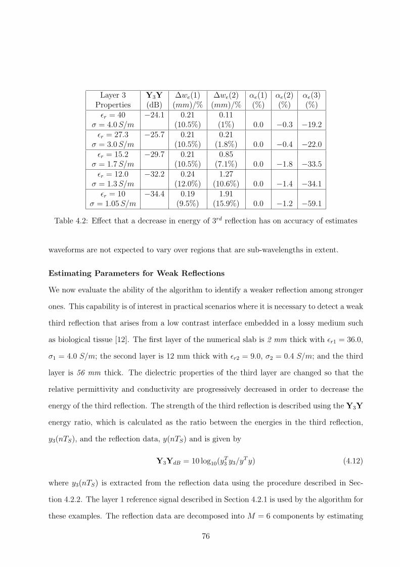
Layer 3 Y3Y ∆we(1) ∆we(2) αe(1) αe(2) αe(3)Properties (dB) (mm)/% (mm)/% (%) (%) (%)ǫr = 40 −24.1 0.21 0.11
σ = 4.0S/m (10.5%) (1%) 0.0 −0.3 −19.2ǫr = 27.3 −25.7 0.21 0.21
σ = 3.0S/m (10.5%) (1.8%) 0.0 −0.4 −22.0ǫr = 15.2 −29.7 0.21 0.85
σ = 1.7S/m (10.5%) (7.1%) 0.0 −1.8 −33.5ǫr = 12.0 −32.2 0.24 1.27
σ = 1.3S/m (12.0%) (10.6%) 0.0 −1.4 −34.1ǫr = 10 −34.4 0.19 1.91
σ = 1.05S/m (9.5%) (15.9%) 0.0 −1.2 −59.1
Table 4.2: Effect that a decrease in energy of 3rd reflection has on accuracy of estimates
waveforms are not expected to vary over regions that are sub-wavelengths in extent.
Estimating Parameters for Weak Reflections
We now evaluate the ability of the algorithm to identify a weaker reflection among stronger
ones. This capability is of interest in practical scenarios where it is necessary to detect a weak
third reflection that arises from a low contrast interface embedded in a lossy medium such
as biological tissue [12]. The first layer of the numerical slab is 2 mm thick with ǫr1 = 36.0,
σ1 = 4.0 S/m; the second layer is 12 mm thick with ǫr2 = 9.0, σ2 = 0.4 S/m; and the third
layer is 56 mm thick. The dielectric properties of the third layer are changed so that the
relative permittivity and conductivity are progressively decreased in order to decrease the
energy of the third reflection. The strength of the third reflection is described using the Y3Y
energy ratio, which is calculated as the ratio between the energies in the third reflection,
y3(nTS), and the reflection data, y(nTS) and is given by
Y3YdB = 10 log10(yT3 y3/y
Ty) (4.12)
where y3(nTS) is extracted from the reflection data using the procedure described in Sec-
tion 4.2.2. The layer 1 reference signal described in Section 4.2.1 is used by the algorithm for
these examples. The reflection data are decomposed into M = 6 components by estimating
76

100
101
102
0
0.5
1
1.5
2
2.5
3
3.5
SNR (dB)
∆we (
mm
)
Figure 4.3: Effect that noise level has on parameter estimation algorithm when estimatingTOA of a weak 3rd reflection.
the TOA and scaling factor of the reflection that arises from each interface. The slab is
illuminated with an UWB differentiated Gaussian pulse having a −3 dB bandwidth of 4.37
GHz (1.14-5.51 GHz). The maximum frequency fmax of the pulse is 7.7 GHz. The weak
reflection test consists of two parts: examining the limits of detection and the robustness to
noise.
First, the energy of the third reflection is progressively decreased by changing the layer
3 dielectric properties; the reflection data are not contaminated with noise samples. The
effect that a decrease in energy of the third reflection has on the precision of the parameters
estimates is shown in Table 4.2. As expected, the third reflection’s strength has no apparent
effect on the quality of the parameter estimates associated with the first two reflections.
However, a Y3Y energy ratio below −32 dB leads to a deterioration in the TOA of the third
reflection and a Y3Y energy ratio below −34 dB leads to a deterioration in the estimation
quality of the third reflection’s amplitude. For breast imaging applications, the scaling
factors associated with the first two reflections may be used to infer the dielectric properties
77

Figure 4.4: Model of three layer slab and sensor used to evaluate the algorithm’s performancewhen applied to 3D numerical data.
of the outer skin layer and fat layer adjacent to the skin. The value of the third scaling factor
is influenced by the dielectric properties of the glandular region. However, this structure is
deeper within the interior of the breast and can be highly heterogeneous. Therefore, it is not
anticipated that the scaling factor of the third reflection is of practical use in the context of
the biomedical problems that this method would be applied to.
For the second part of this test, the dielectric properties of the third layer are fixed to
ǫr3 = 10.0, σ3 = 1.05 S/m to simulate a low contrast interface scenario and contaminate the
reflection data with noise samples from the WGN model and progressively lower the SNR.
The error in the estimated thickness of the third layer versus the SNR is shown in Fig. 4.3.
The graph suggests that the estimated TOA of the third reflection is robust to the presence
of noise at levels 10 dB and above; but, starting at 5 dB, a significant deterioration in the
quality of these estimates occurs.
In a practical scenario there is uncertainty in the number of interfaces that an object
contains which typically means that the model order in (4.2) is not known a priori. Due
to the damped nature of the reflected signals, information theoretic techniques [127], and
Bayesian MMSE estimators [128] are unsuccessful in estimating this parameter. This is
also observed in [129]. We investigated the effect that model order mismatch has on the
78

1.4 1.6 1.8 2 2.2 2.4
x 10−9
−1
−0.5
0
0.5
1
time (s)
Nor
mal
ized
am
plitu
de
y(nTs)
r(nTs)
(a)
1.4 1.6 1.8 2 2.2 2.4
x 10−9
−1
−0.5
0
0.5
1
time (s)
Nor
mal
ized
am
plitu
de
Actual reflection 1Actual reflection 2Actual reflection 3
(b)
1.4 1.6 1.8 2 2.2 2.4
x 10−9
−1
−0.5
0
0.5
1
time (s)
Nor
mal
ized
am
plitu
de
Est. reflection 1Est. reflection 2Est. reflection 3
(c)
Figure 4.5: (a) Reflection data, y(nTS), shown in blue are contaminated with colored noisesamples such that the SNR is 20 dB. The reference signal, r(nTS) used by algorithm is shownin red. (b) Corresponding reflections that arise from the three interfaces. (c) Estimates ofeach reflection. A significant overlap between the 1st two reflections and a weak 3rd reflectionare observed.
accuracy of the estimates and found that accurate estimation of the model order is not
required. The algorithm is generally robust to large deviations from the correct model order;
but overestimation of the model order typically leads to more accurate model parameter
estimates than underestimation of the model order. This is also observed in [119], provided
that the order of the noise model is set to zero.
79

∆we(1) ∆we(2) αe(1) αe(2) αe(3)(mm)/% (mm)/% (%) (%) (%)
0.08 −0.73(4.0%) (−4.0%) −5.3 1.6 0.3
Table 4.3: Thickness error for each layer of 3D numerical slab. The first layer is 2 mm andthe 2nd layer is 18 mm which corresponds to a reflection overlap of B∆T = 0.28 and 1.27,respectively.
4.3 Application of the algorithm to 3D numerical data
This test investigates the performance of the algorithm when applied to numerical data gen-
erated with a 3D slab using a realistic source/sensor model. The simulations are carried
out with the finite-difference-time-domain method using SEMCAD X (SPEAG AG, Switzer-
land). A stratified and non-dispersive dielectric slab is placed within the simulation space
as shown in Fig. 4.4. The thin outer layer closest to the source/sensor is 2 mm thick with
ǫr1 = 36.0, σ1 = 4.0 S/m; the middle layer is 18 mm thick with ǫr2 = 9.0, σ2 = 0.4 S/m;
and the third layer extends to infinity (i.e., is terminated with a PML) with ǫr3 = 30.0,
σ3 = 3.0 S/m. Both the slab and source/sensor are located in an immersion liquid with
ǫr = 3.0, σ = 0.04 S/m. A Balanced Antipodal Vivaldi antenna with director (BAVA-D)
[66] is placed 25 mm from the slab, illuminates the slab, and records the resulting backscat-
tered fields. The illuminating UWB pulse has a −3 dB bandwidth of 3.5 GHz (1/B ≈ 0.286
ns) and fmax = 7.7GHz. To evaluate if the algorithm is robust to the presence of noise
in the data, noise samples from a colored noise process obtained by filtering a Gaussian
process are added to the reflected data such that the SNR is 20 dB. The reference signal is
acquired using the procedure described in Section 4.2.1 with the dielectric slab having the
same properties as the first layer. The number of samples is N = 2211 and the sample time
is TS = 1.81 ps. A model order of M = 4 is assumed.
Figure 4.5 shows an example of the reference signal used for these examples and data
contaminated with colored noise samples. The reflections from each interface used to eval-
80

(a) (b)
Figure 4.6: (a) Experimental apparatus used to test RDD algorithm. (b) Top view of tankshowing dielectric slabs immersed in Canola oil with UWB sensor.
uate the performance are extracted using the procedure described in Section 4.2.2. These
reflections are shown in Fig. 4.5(b) where we observe significant overlap between the first
two reflections (B∆T = 0.28) and a weak third reflection (Y3Y = −24.7 dB) relative to the
other reflections.
The estimated reflections corresponding to the three interfaces for this example are shown
in Fig. 4.5(c). The thickness error for each layer is shown in Table 4.3, demonstrating that
the sub-mm accuracy noted in the 2D case is also achieved in 3D. The 3D results related
to layer 1 are in agreement with the 2D case where B∆T = 0.29 as shown in Table I; the
3D results related to layer 2 are in agreement with the 2D case where Y3Y = −25.7 dB as
shown in Table 4.2.
For the example related to Fig. 4.5(b), we observe that a discrepancy exists between the
waveform shapes of the first and second reflections. This leads to the presence of artifacts
in the residue after the estimates of the first and second reflections are removed from Y to
compute Y3 in step 3.1 of the RDD algorithm (described in Section 4.1). The results suggest
that the effect that this phenomenon has on the TOA estimate is marginal. However, this
phenomenon is important if the criterion is to accurately estimate the first two reflections.
81

Layer Properties Actual B∆T thicknessThickness error
(mm) mm/(%)1 ǫr = 34.3 0.60
σ = 4.25S/m 1.7 0.21 (35.3%)2 ǫr = 12.0 −0.28
σ ≈ 0.05 − 0.2S/m 9.8 0.70 (−2.86%)
Table 4.4: Thickness error for each layer of a 2 layer slab consisting of a very thin skin layerover a dielectric slab.
4.4 Application of algorithm to experimental data
4.4.1 Experimental apparatus
The performance of the method is tested further by applying it to experimental data collected
using the apparatus shown in Fig. 4.6. The setup consists of a tank containing an immersion
liquid, a sensor (BAVA-D antenna [66]) and layered objects or slabs. Canola oil is used as the
immersion liquid with ǫr = 2.5, σ ≈ 0.04S/m. The reference signal is acquired by inserting
a metal plate in the tank at 35 mm from the antenna.
Measurements are obtained with the antenna placed 25 mm in front of the slabs. For all
cases, measurement data are collected at 1601 points over the frequency range from 50 MHz
to 15 GHz using a Vector Network Analyzer (VNA) (8722ES, Agilent Technologies, Palo Alto,
CA). The VNA IF bandwidth is adjusted to 1000 Hz and averaging is set to 3 sweeps per
measurement. The frequency domain VNA measurements are weighted with a differentiated
Gaussian signal with a −3 dB bandwidth of 3.11GHz (1/B ≈ 0.322 ns ≈ 160TS), then
transformed to time-domain data with an inverse chirp-z transform described in [130]. The
resulting time-domain signal has N = 1751 samples and the sample time is TS = 2.00 ps.
Two experimental cases are studied. For the first case, a two layer slab is formed by
placing a 1.7 mm thick skin layer with ǫr1 = 34.3, σ1 = 4.25 S/m (averaged over 1.0
to 10 GHz) over a 9.8 mm thick dielectric slab with ǫr2 = 12.0, σ2 ≈ 0.05 − 0.2 S/m
82

0.8 1 1.2 1.4 1.6 1.8 2 2.2
x 10−9
−1
−0.5
0
0.5
1
time (s)
Nor
mal
ized
am
plitu
de
r(nTs)
y(nTs)
(a)
0.8 1 1.2 1.4 1.6 1.8 2 2.2
x 10−9
−1
−0.5
0
0.5
1
Time (s)
Nor
mal
ized
Am
plitu
de
Est. reflection 1Est. reflection 2Est. reflection 3
(b)
Figure 4.7: (a) Reflection data, y(nTS), acquired from dielectric slab covered by thin skinlayer, and metal plate reference signal, r(nTS), used by algorithm, and (b) correspondingestimates of reflections arising from the three interfaces. Overlap between all three of theestimated reflections is observed.
(Eccostock HiK, Emerson and Cuming Microwave Products Randolph, MA, USA). The
skin layer is constructed of silicone with dielectric fillers (LDF-32, Emerson and Cuming
Microwave Products) having dispersive properties. A reference signal is acquired by recording
the reflection from a metal plate placed 10 mm from the sensor.
For the second case, the slab consists of three layers formed by sandwiching a 13.0 mm
dielectric slab with ǫr2 = 6.0, σ2 ≈ 0.05 − 0.2S/m between a two 9.8 mm thick dielectric
slabs with properties of ǫr1 = 12.0, σ1 ≈ 0.05− 0.2S/m and ǫr3 = 10.0, σ3 ≈ 0.05− 0.2S/m,
respectively. The slabs are Eccostock HiK (Emerson and Cuming Microwave Products).
83

4.4.2 Experimental results
For the two layer slab, which is the first case, the reflection data that the parameter es-
timation algorithm operates on and the reference signal used by the algorithm are shown
in Fig. 4.7(a). The reflection data are decomposed into M = 6 components, estimated
reflections associated with each interface are shown in Fig. 4.7(b) and the corresponding
layer thickness evaluations are shown in Table 4.4. Sub-mm precision is observed for both
thickness estimates. Moreover, very accurate estimation of the second 9.8 mm slab layer is
achieved regardless of the overlap between the second and third reflections implied by the
B∆T product. We also observe this overlap between the estimated reflections in Fig. 4.7(b).
This is a critical result that supports the validity of applying the algorithm to the near-field
application of estimating the skin thickness, estimating the skin response, and estimating
the distance to an interface associated with the adipose/fibroglandular boundary.
For the three layer slab, which is the second case, the reflection data and the reference
signal used by the algorithm are shown in Fig. 4.8(a). The reflection data are decomposed
into M = 6 components and the four estimated reflections that arise from the four interfaces
are shown in Fig. 4.8(b). The TOA of the estimated reflections used to evaluate the layer
thicknesses are shown in Table 4.5. Although each layer is thinner than the resolution limit
of a matched filter, the layer thicknesses are estimated with sub-mm accuracy. As with the
2D and 3D simulated cases, the very accurate estimation of each slab’s thickness is achieved
regardless of the overlap of the reflections. Importantly, this general example demonstrates
the algorithm’s ability to accurately estimate the parameters of multiple reflections associated
with several closely spaced interfaces.
4.4.3 Experimental results discussion
In [113] and [131], a high-resolution algorithm for B∆T = 0.42, 0.84 and 1.26 was exper-
imentally tested; in [114] the authors experimentally tested a high-resolution algorithm for
84

Layer Properties Actual B∆T thicknessThickness error
(mm) mm/(%)1 ǫr = 12.0 −0.11
σ ≈ 0.05 − 0.2S/m 9.8 0.70 (−1.09)2 ǫr = 6.0 0.11
σ ≈ 0.05 − 0.2S/m 9.8 0.50 (1.16)3 ǫr = 10.0 −0.11
σ ≈ 0.05 − 0.2S/m 13.0 0.85 (−0.82)
Table 4.5: Thickness errors of 3 layer slab used to evaluate algorithm’s performance whenapplied to experimental data. TOA from 4 reflections are required to estimate thickness ofthe 3 layers.
B∆T = 4.6 and 1.7. By experimentally investigating the high-resolution capability of the
algorithm for a scenario where B∆T = 0.21, we evaluate the capability of the algorithm to
experimentally resolve reflections having a greater degree of overlap than previously pub-
lished results.
For the dispersive skin layer, sub-mm precision of the skin’s estimated thickness is
achieved regardless of the extreme overlap between the 1st and 2nd reflections which is implied
by the B∆T value of 0.21. This result is in close agreement with a similar case examined
in Section 4.2.3 in which two overlapping signals where B∆T = 0.21 (Table 4.1) are re-
solved. This suggests that thin layers of dispersive materials may not lead to deterioration
of the algorithm’s performance since preservation of the waveform shape is expected over
regions that are sub-wavelengths in extent. We anticipate that scenarios where the material
is both dispersive and has a large extent relative to the wavelength of the incident pulse
may adversely affect the performance of the algorithm. For these situations, the reference
signal r(nTS) must take into account the dispersive effects of the medium. We are presently
investigating methods to achieve this.
Since the reflection from a metal plate is used to construct the reference signal, the
experimental results also support the conclusion drawn for the 2D case that the algorithm
85
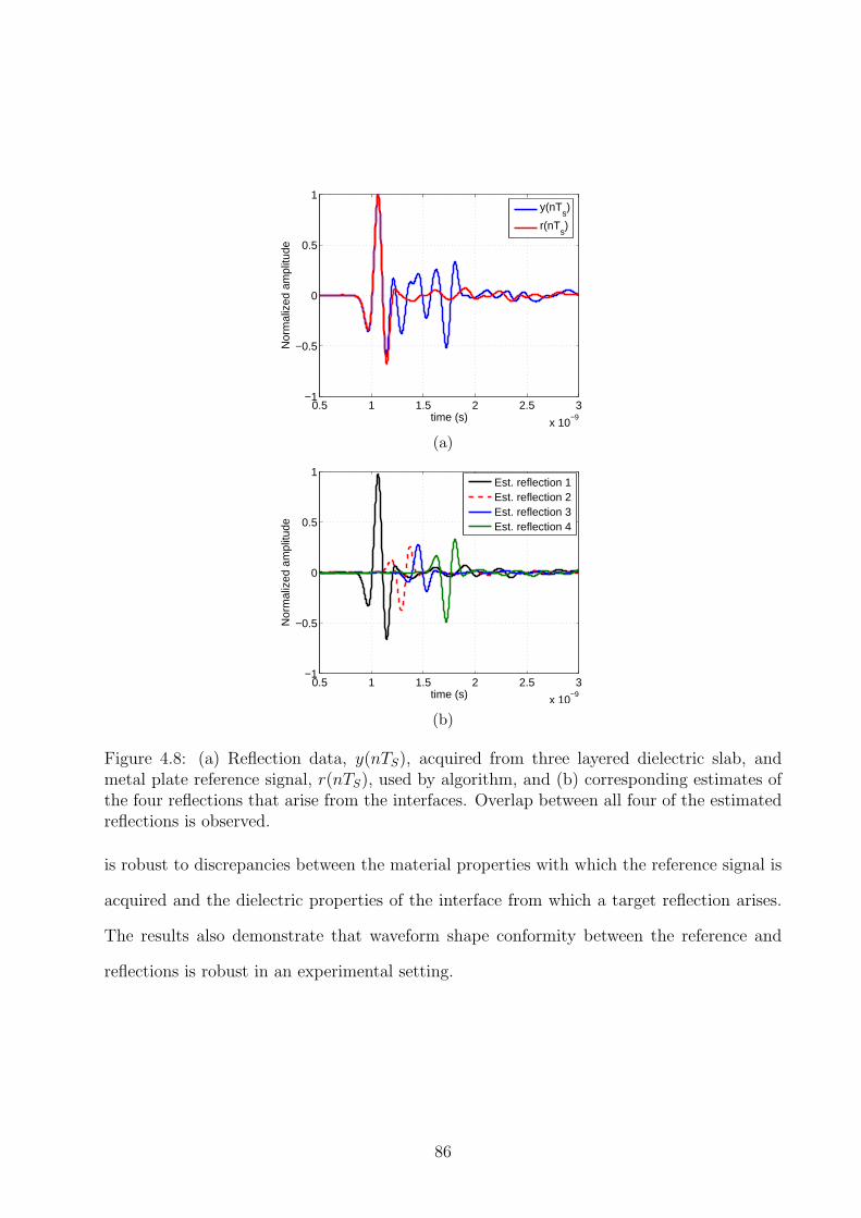
0.5 1 1.5 2 2.5 3
x 10−9
−1
−0.5
0
0.5
1
time (s)
Nor
mal
ized
am
plitu
de
y(nTs)
r(nTs)
(a)
0.5 1 1.5 2 2.5 3
x 10−9
−1
−0.5
0
0.5
1
time (s)
Nor
mal
ized
am
plitu
de
Est. reflection 1Est. reflection 2Est. reflection 3Est. reflection 4
(b)
Figure 4.8: (a) Reflection data, y(nTS), acquired from three layered dielectric slab, andmetal plate reference signal, r(nTS), used by algorithm, and (b) corresponding estimates ofthe four reflections that arise from the interfaces. Overlap between all four of the estimatedreflections is observed.
is robust to discrepancies between the material properties with which the reference signal is
acquired and the dielectric properties of the interface from which a target reflection arises.
The results also demonstrate that waveform shape conformity between the reference and
reflections is robust in an experimental setting.
86

4.5 Discussion and concluding remarks
A high-resolution parameter estimation algorithm has been presented that may be used for
near-field applications to decompose severely overlapping reflections contaminated with noise
that arise from interfaces that are closely spaced relative to the illuminating wavelength. The
algorithm does not assume exact knowledge of the transmitting signal, but uses a reference
signal selected to adapt to the physical behavior exhibited for near-field applications. Impor-
tantly, the waveform shape of the reference is robust to discrepancies between the material
properties for which the reference signal is acquired and the dielectric properties of the in-
terface from which a target reflection arises. Furthermore, the algorithm is robust to the
presence of noise at low signal-to-noise levels.
The numerical results obtained using the realistic UWB sensor demonstrate performance
features critical to near-field applications, namely the ability to accurately estimate param-
eters associated with two severely overlapping reflections contaminated with noise as well
as the capability to accurately estimate the parameters associated with a weak reflection.
Moreover, these numerical results support the 2D findings, suggesting that the near-field
2D performance tests can be extended to an equivalent near-field 3D scenario that uses a
realistic sensor model. The results also demonstrate that the algorithm’s performance is
not adversely affected by colored noise SNR of 20 dB. We also note that these numerical
results are comparable to those presented in literature (e.g. [113][114]); but we define the
bandwidth of the signal at −3 dB which means that the B∆T values investigated in this
paper are much lower than an equivalent value presented in [113] or [114], as these references
define the bandwidth of the signal at −6 dB and −10 dB, respectively.
All numerical and experimental data sets are generated with planar slabs that have abrupt
and ’smooth’ boundaries (i.e., no spatial variations of the boundary relative to the wavelength
of the illuminating signal) so the effects that arise due to the multipath phenomena are
minimized. We anticipate that this phenomenon may be observed for scenarios where the
87
boundaries are curved and irregularly shaped. The signal model given by (4.1) assumes
that each reflection corresponds to a single scattering event from a medium interface so the
multipath phenomena violate this assumption. One approach to resolving the multipath
problem is to use multiple antennas to provide multiple views of the boundaries. We are
presently investigating and developing these techniques.
Although this is a general algorithm, it is suitable for near-field applications to evaluate
the thickness of thin layers. For example, knowledge of the skin thickness is critical when
microwave tomographic and radar imaging algorithms are used for breast tissue property
reconstruction and for tumor detection and localization. Moreover, the algorithm is exper-
imentally evaluated with a thin layer that leads to a smaller B∆T (B∆T = 0.21) than
reported in literature using other high-resolution algorithms (e.g., [113], [114] and [131]).
The algorithm’s ability to accurately estimate the parameters of multiple reflections associ-
ated with several closely spaced interfaces in a more general practical setting demonstrates
the algorithm’s broader applicability.
The RDD algorithm has been developed such that it is capable of decomposing reflection
data by estimating reflections of interest in the microwave breast imaging application. In-
formation from each modeled reflection is used to estimate the extent of regions such as the
thickness of skin and the skin-to-gland layer distance. In Chapter 5, the RDD algorithm is
applied to reflections collected as an antenna scans an object. The estimated extent of each
region extracted at each antenna is mapped to points (or samples) on interfaces between dif-
ferent regions. The points are then used to estimate the shape of an interface that segments
two distinct regions.
88

Chapter 5
Extraction of internal spatial features of
inhomogeneous dielectric objects
3 Evaluating interface samples is the second of a three step procedure used to form a recon-
struction model. In this chapter, the RDD algorithm is applied to reflection data acquired
from a source/sensor scanned to multiple locations around an object. A method is presented
that transforms the estimated time-of-arrival (TOA) parameters associated with each mod-
eled reflection to points on contours or interfaces. The sequence of points are referred to as
contour samples and may be used to estimate the shape of an interface that segregates and
encloses a region of dissimilar dielectric properties within the object. These regions collec-
tively form an object-specific reconstruction model that segments the interior into regions
and is incorporated into MWT. This permits the mean dielectric properties to be estimated
over each region and to provide insights into the underlying structure of the object. The
integration of the reconstruction model into microwave tomography is described in Chapter
6. In the context of breast MWI, unlike other methods such as the soft-priors [105], this
technique acquires this information using a single modality. In this chapter, the possibility
of enhancing the RDD algorithm by incorporating prior information about the target into
the reference functions is also explored. The method that evaluates the contour samples
is described in Section 5.1. The technique is applied to 2D numerical models of increasing
complexity in Section 5.2. Finally, the algorithm is applied to breast models based on MR
scans in Section 5.3, suggesting the feasibility of delineating regions dominated by fat and
glandular tissues.
3This chapter is adapted from D. Kurrant and E. Fear,“Extraction of internal spatial features of inhomo-geneous dielectric objects using near-field reflection data”,Prog. Electromagn. Res., vol. 122, pp. 197-221,2012.
89

P 0
i
01
12 23
P 12
( i ) P
23
( i )
P ( i ) A
S
1
2
3
v
Figure 5.1: A region Ω with known dielectric properties is bounded by N sources/sensors(dots) co-located on its boundary ∂Ω. Contained within the measurement region is a di-electric object S covered by a thin layer (Σ1) with ǫr1, σ1. The interior of the object hastwo regions (Σ2, Σ3) with dissimilar properties ǫr2, σ2 and ǫr3, σ3, respectively. The problemconsidered here is to evaluate points PΓ12
(i) and PΓ23(i) on contours Γ12 and Γ23, respectively.
5.1 Methods
We begin with a general description of the problem. Consider an inhomogeneous dielectric
object S shown in Fig. 5.1 covered by a thin layer which we denote as region 1 (Σ1). The
interior consists of two regions, labeled Σ2 and Σ3, having dissimilar dielectric properties.
We position the object within a bounded 2D homogeneous measurement region, Ω. The
interfaces between regions are denoted as Γ01, Γ12 and Γ23, respectively. We note that for
the breast imaging application, region 1 represents skin, while regions 2 and 3 represent
regions dominated by adipose and glandular tissues, respectively. These interior regions are
not restricted to be homogeneous, but rather represent regions that are dominated by a
particular tissue type.
A source element illuminates Ω with an UWB electromagnetic pulse, while the sensor at
the same location as the source records the backscattered signals. A full set of data collection
using this configuration consists of moving the source and sensor pair to N equally spaced
90

locations on the boundary of the measurement region. The locations of the sensors and
contour Γ01, as well as the dielectric properties of region Ω are known a priori. Furthermore,
we assume that the relative permittivity of regions 1 and 2 is estimated beforehand using a
technique presented in Chapter 6.
For each sensor position, the reflected field information is used to estimate the points
PΓ12(i) and PΓ23
(i) on contours Γ12 and Γ23, respectively. Repeating this procedure for N
sensors leads to a sequence of points which we refer to as contour samples that may be
used to estimate contours Γ12 and Γ23. The methodology we have developed to identify
the reflection that arises from each interface is described in Section 5.1.1. Each reflection is
characterized by its scaling factor and TOA. The TOA is used to estimate the location on
the contour from which the reflection originated, as described in Section 5.1.2.
5.1.1 Estimating amplitude and TOA of each reflection
The object in Fig. 5.1 is illuminated by an UWB pulse and a single sensor receives the
reflected signal. The data received by the sensor are conditioned so that the transmitted
signal is removed from the reflection data. As discussed in Chapter 4, the pre-conditioned
data, y(t), are modeled as a superposition of scaled and delayed replicas of a reference signal
r(t) plus noise:
y(t) =M∑
m=1
αmr(t− τm) + e(t), 0 ≤ t ≤ T (5.1)
where M is the number of replicas of r(t); αm and τm are the scaling factor and TOA of the
mth replica, respectively; T is the duration of the signal; and e(t) is noise modeled as a zero-
mean Gaussian random process. Each of scaled and time-delayed version of the reference
signal models a reflection from an interface separating the object’s different dielectric regions.
The RDD algorithm is applied to a given backscattered signal to estimate values for the
scaling factors and TOAs, as discussed in Chapter 4. The TOA information may be used to
infer the location of an interface. Although it is not investigated in this study, the scaling
91

Figure 5.2: Flow-chart of the three-step procedure used to estimate the scaling factor αand TOA parameter τ for each reflection contained in the backscattered data y(t). Each ofscaled and time-delayed version of the reference signal models a reflection from an interfaceseparating the object’s different dielectric regions. At each step, prior information aboutan interface (e.g., geometrical and/or dielectric properties) may be incorporated into thereference signal ri(t).
factor may be used to infer the dielectric properties of a region.
Since prior information may be available for each interface, the reference signal used in
(5.1) may incorporate this information. Accordingly, the algorithm is adapted to use mul-
tiple reference signals (i.e., one reference signal for each interface) to estimate reflections
contained in the recorded data using the three step procedure shown in Fig. 5.2. The moti-
vation for using this methodology is that additional prior information may be incorporated
into each reference signal to improve the accuracy of the reflection model from an interface.
For example, if the dielectric properties of an object’s surface are known beforehand, then a
reference object having these properties may be used to create a reference signal used specifi-
92

cally to model the surface reflection. In this case, for the first step of the RDD algorithm, this
first reference, r1(t), is used to estimate the surface reflection leading to y1(t) = α1r1(t− τ1).
The estimate of the surface reflection is then removed from the backscattered data (i.e.,
g2(t) = y(t) − y1(t)). If additional prior information is known such as the object is covered
by a thin outer skin, then reference objects may be selected to generate a second reference
signal, r2(t), appropriate for modeling the reflection from the skin/fat interface. For the sec-
ond step, the RDD algorithm is applied to g2(t) using r2(t) to estimate the reflection from
the skin/fat interface to yield y2(t) = α2r2(t − τ2). The estimate of the skin/fat interface
reflection is then removed from g2(t) (i.e., g3(t) = g2(t) − y2(t)). Finally, if additional prior
information is known about the third interface, then reference objects may be selected to
generate a third reference signal. For the third and final step of the algorithm, the RDD
algorithm is applied to g3(t) using r3(t) to estimate the reflection from the fat/glandular
interface resulting in y3(t) = α3r3(t− τ3).
The multiple reference function approach may also be used to accommodate reference
functions with different frequency contents. For example, when imaging the breast at mi-
crowave frequencies, the spectral content of the illuminating signal is an important consider-
ation. On one hand, an illuminating signal with higher frequency components (≈12.5 GHz)
is required to resolve the skin thickness. However, higher losses at these frequencies lead to
poor depth of penetration, so the use of this signal is restricted to extracting information
related to thin structures close to the surface (e.g, the skin). On the other hand, identify-
ing interfaces deeper within the breast requires an illuminating signal with lower frequency
components in order to improve the depth of penetration. Unfortunately, the improvement
in depth of penetration of the signal comes at the expense of loss of resolution. Therefore,
we propose a sequential estimation procedure that preserves resolution while enhancing pen-
etration. The object is first illuminated with a signal having higher frequency components
leading to backscattered data, yh(t). Reference functions are also generated for this sig-
93

nal (e.g., r1,h(t), r2,h(t), r3,h(t)) and are used to decompose the reflections contained in the
backscattered data. The TOA estimates for the first two reflections are used to evaluate the
skin thickness. Next, an illuminating signal with frequency components lower than the first
illuminating signal is used yielding backscattered data yl(t). The decomposition procedure
is applied to the backscattered data, yl(t), using reference signals generated for this second
excitation (e.g., r1,l(t), r2,l(t), r3,l(t)). Although the first three reflections are estimated, only
the estimated reflection from the fat/glandular interface is used. In particular, the TOA
estimated for the third reflection of the low frequency data, and the TOA estimated for the
second reflection of the high frequency data are used to estimate the distance from contour
Γ12 to Γ23 which extends into lossy tissue. The procedure used to estimate the extent of a
region using the TOA estimates is described in Section 5.1.2.
5.1.2 Evaluating interface samples
Once the recorded reflection signal is decomposed into M components, estimates of the
TOAs and scaling factors of the reflections that arise from each interface are available.
This information is first used to estimate the extent of each region near each antenna. The
estimates from all sensors are then used to identify points on contours separating the regions.
The TOA is used to estimate the thickness or extent of each region with the assumption
that the average permittivity of each region is known. For sensor i, the extent of region j is
estimated using the difference in TOA between successive reflections:
∆τj(i) = τj+1(i) − τj(i). (5.2)
Specifically, the thickness of layer j near antenna i, wj(i), is estimated as:
wj(i) =∆τj(i)c0103
2√ǫrj
. (mm) (5.3)
where c0 = 2.9979 × 10⁸ m/s is the speed of light in free space and ǫrj is the estimated
average relative permittivity of the jth region of interest. We note that a more accurate
94
formula that takes into consideration the conductivity may be used to calculate the phase
constant which, in turn, is used to estimate the phase velocity. However, this leads to a
marginal improvement in the accuracy of the skin thickness estimate (e.g., for an actual skin
thickness of 2.12 mm, the estimated skin thickness using (5.3) is 2.28 mm (7.5 % error) and
the estimated skin thickness using the more accurate estimate of phase velocity is 2.17 mm
(2.3 % error)). For the adipose region, the estimated distance between interfaces is much
larger compared to the skin thickness and the conductivity is typically an order of magnitude
smaller than the conductivity for skin. Hence, using a more accurate expression for velocity
to calculate the distance leads to a negligible difference in results. For this study, satisfactory
accuracy of the distances is provided using the average relative velocity.
Next, an iterative procedure uses the layer thicknesses in conjunction with a line-of-sight
ray connecting the sensor to the center of the region of interest (ROI). The center of the ROI
is identified as point P0 as shown in Fig 5.1. The location of sensor i is known and described
as point PA(i) with PA,x(i) and PA,y(i) denoting the x and y-coordinates, respectively. The
distance from the ith antenna to the outer surface of the object, w0(i), is also assumed to be
known a priori.
Consider the contour separating regions 1 and 2 (Γ12). The distance from antenna i to a
point on this contour is given by:
wΓ12(i) = w0(i) + w1(i). (mm) (5.4)
This distance is used to estimate the coordinates of the point PΓ12(i) on the contour. As
shown in Fig. 5.1, a line-of-sight ray connects the ith sensor at point PA(i) with the center
of the ROI at point P0. A direction vector ~v along the ray points to the center and is
incorporated into the vector parametric equation of the ray:
~PΓ12(i) = ~PΓA
(i) + t~v (5.5)
where ~PΓ12(i) is the position vector of the point PΓ12
(i) on the contour, ~PA(i) is the position
vector of the location of the ith antenna, and t ∈ [0, 1]. When t = 0, PΓ12(i)=PΓA
(i); when t
95
= 1, PΓ12(i)=P0. The expression given by (5.5) is constrained by
wΓ12(i) =
√(PA,x(i) − PΓ12,x
(i))2 + (PA,y(i) − PΓ12,y(i))2 (5.6)
where PΓ12,x(i), PΓ12,y
(i) are the x and y-coordinates of PΓ12(i), respectively. The coordinates
of PΓ12(i) are determined iteratively using (5.5) and (5.6) with the following procedure. Scalar
t is incrementally increased to move the position vector point ~PΓ12(i) along the line-of-sight
ray given by (5.5) until the distance traveled by the point satisfies the distance given by (5.6).
This process is repeated for all N sensors in order to form a sequence of points PΓ12(1), . . . ,
PΓ12(N) which estimate N locations along the contour Γ12.
We repeat this process to determine the coordinates of the point PΓ23(i) on the estimated
location of contour Γ23. In this case, the distance from antenna i to a point on the contour
Γ23 is estimated with
wΓ23(i) = wΓ12
(i) + w2(i). (mm) (5.7)
We refer to this entire procedure as the contour sample evaluation algorithm. The se-
quence of 2N points may be used to infer the basic shapes of contours Γ12 and Γ23 (i.e.,
geometrical properties) and of the object’s interior regions. Hence, this information may
be used to approximate the object’s internal structure. Although we restrict this technique
to the identification of just three regions for this investigation, it can be easily extended to
extract contour information related to more than three regions.
5.2 Initial performance evaluation
The ability of the algorithm to extract an object’s internal geometrical properties is evalu-
ated with a 2D object having progressively more complex regional shapes. Furthermore, the
results are compared as more a priori information about the regional properties is incorpo-
rated into the reference signals. The approach used to generate the numerical data and the
metrics used to evaluate the performance of the algorithm are described in Section 5.2.1 and
96

Section 5.2.2, respectively. The results and performance of the algorithm are described in
Section 5.2.3.
5.2.1 Generation of Numerical Data
Numerical simulations using the FDTD method are used to generate test data. In these
examples, the FDTD problem space is bounded by a five-cell thick perfectly matched layer
(PML) boundary (4th order, R(0) = 10−7) with spatial grid resolution of 0.5 mm. Similar
to the illustration in Fig. 5.1, a model having three distinct homogeneous regions is placed
within the problem space. The sensor and source are co-located 10 mm from the surface of
the outer layer. Both the model and source/sensor are located in free space. An impressed
current source is used in these TMx simulations. A pulse is used for the time-domain
excitation function,
S(t) = s0(t− t0) exp(−(t− t0)2/τ 2), (5.8)
where s0 is a scalar, t0 is the centre of the pulse in time, and τ is a variable that controls
the rise time of the pulse. The value of τ is adjusted so that the pulse has the required
maximum frequency, fmax, content. Here, fmax, is the frequency of the spectrum where the
magnitude of S(ω) is 10% of its maximum magnitude. In all of the examples, the number
of samples is NS = 4000 and the sample time is TS = 1.06 ps.
When generating the numerical data, reflections are recorded as the sensor is scanned to
20 equally spaced locations around the model. The incident field is acquired by carrying out
a simulation without the model. Data received by the sensor are conditioned such that the
incident field is removed from each reflection. The data are then normalized to the reflected
signal’s maximum positive value and are contaminated with zero-mean white Gaussian noise
samples such that the SNR is 20 dB. Here, SNR is defined as the ratio of the signal energy
to the total energy of the noise process. Therefore, a SNR of 20 dB means that the signal
energy is 20 dB above the energy of noise process.
97

5.2.2 Assessing the performance of the algorithm
To assess the performance of the contour sample evaluation algorithm, the actual reflections
from each of the three interfaces (Fig. 5.1) are isolated in order to extract actual values of the
scaling factors and TOAs. The procedure has been described already in Chapter 4, however,
it is repeated here again for clarity. First, a simulation is carried out with a homogeneous
model (i.e., entire model has the same properties as the outer layer) to provide an isolated
version of the reflection from the first interface, y1(t). The reflection is normalized by the
positive maximum of the reflection, then characterized by the scaling factor, α1 = 1.0, and
TOA τ1 which is the time that the positive maximum occurs. Next, a simulation is carried
out with the third region replaced with a dielectric material having the same properties as the
second region and this signal is used to isolate the reflection from the second interface, y2(t).
After normalizing to the first reflection, the scaling factor α2 and TOA τ2 are determined.
Finally, a third simulation is carried out with the three region model. The first two reflections
are subtracted from the resulting data, isolating the reflection from the third interface, y3(t).
After normalizing to the first reflection, the resulting signal is characterized by the scaling
factor α3 and TOA τ3.
The error in TOA is explored by comparing actual and estimated differences in successive
TOA estimates. Specifically, the error, ∆τe(i), is calculated by subtracting the actual from
the estimated ∆τ(i) of the reflections. Rather than examining the error in TOA directly,
the spatial error, ∆wej(i), for the jth layer is of greater practical interest and is calculated
using,
∆wej(i) =∆τe(i)c0103
2√ǫrj
(mm) for j = 1, 2 (5.9)
where ǫrj is the average relative permittivity of the jth layer. The thickness error for the jth
layer is then calculated relative to the actual layer thickness. Likewise, the relative error for
each of the reflection amplitudes is computed using
αej(i) =αj(i) − αj(i)
|αj(i)|for j = 1, 2 (5.10)
98

z (mm)
y (m
m)
50 100 150 200
50
100
150
200 5
10
15
20
25
30
35
εr
Figure 5.3: Relative permittivity profile of model 1. The skin layer is 2 mm thick with ǫr1= 36.0, σ1 = 4.0 S/m; the middle layer is 14 mm thick with ǫr2 = 9.0, σ2 = 0.4 S/m; andthe center region has a radius of 24 mm with ǫr3 = 40.0, σ3 = 3.2 S/m.
where αj(i) is the estimated value of the jth scaling factor. We note that the absolute
difference in TOA and α may also be used in (5.9) and (5.10), respectively, as a metric
to evaluate the accuracy of the estimator. We have not chosen this approach since we are
interested in determining if the parameter is being overestimated or underestimated. This
is discussed further in Section 5.2.3.
The similarity between the estimate of a reflection, yj(i), and the actual reflection is
computed using:
ρj =yT
j yj
‖yj‖‖yj‖for j = 1, 2, 3. (5.11)
A value close to 1 indicates a close similarity between the estimate of the reflection and the
actual reflection.
Each performance measure is averaged over all N sensors.
5.2.3 Results
We first evaluate the performance of the algorithm for a base-line case whereby the object
has a simple cylindrical shape and limited a priori information about the object is available.
99

Ref. Slab prop. ∆we1 ∆we2
ǫr σ (S/m) mm/ mm/ αe1 αe2 ρ1 ρ2 ρ3
(%) (%) (%) (%)36 4 0.12 -0.01 0.8 -0.4 0.9996 0.9419 0.7078
(6%) (-0.1%)43.2 4.8 0.11 -0.003 0.8 -4.2 0.9996 0.9415 0.7119
(6%) (-0.02%)28.8 3.2 0.11 0.007 0.8 -3.6 0.9996 0.9417 0.7048
(6%) (0.05%)
Table 5.1: Effect that a discrepancy between the properties used to acquire the referencesignal and the actual properties of the model has on performance of the reflection datadecomposition algorithm. A single reference signal is used. The actual skin properties formodel 1 are ǫr = 36 σ = 4.0 The performance measures are averaged over all 20 antennas.
The same reference signal is used for all three steps of the parameter estimation algorithm for
Case 1. For Case 2, a priori information about both the thickness and dielectric properties
of the outer layer (skin region) is used to refine the second reference signal. Finally, the
performance of the algorithm is evaluated when the skin region and the object’s interior
have more complicated geometrical properties as described for Case 3.
Case 1: Object with simple cylindrical shape
A three layer cylinder is used to evaluate the effectiveness of the contour sample evaluation
algorithm for an object with a geometrically simple internal structure. The model is shown
in Fig. 5.3. Region 1 is a simplified representation of skin and will be referred to as the skin
layer. The cylinder is illuminated with an UWB differentiated Gaussian pulse having a -3dB
bandwidth of 4.62 GHz (1.62 - 6.24 GHz). The maximum frequency fmax of the pulse is
8.59 GHz.
To test the algorithm’s robustness to variations between the reference signal and model,
several scenarios are investigated. First, the reference signal is acquired by simulating a
homogeneous planar layer (slab) having dielectric properties of ǫr = 36.0, σ = 4.0 S/m.
Next, reference signals are constructed using reflections from dielectric slabs with properties
100

of ǫr = 28.8, σ = 3.2 S/m (i.e., the dielectric properties of the slab are −20% of the actual
properties), and ǫr = 43.2, σ = 4.8 S/m (i.e., the dielectric properties of the slab are +20%
of the actual properties). For these cases, the reflection from the slab is normalized and used
for all three reference signals in the reflection decomposition algorithm shown in Fig. 5.2.
Table 5.1 summarizes the results obtained for each of the three reference signals. First,
we examine the average error of the skin layer thickness, ∆we1, and the average error in the
skin-to-region 3 distance, ∆we2. These errors are very small for all cases, suggesting that the
algorithm is able to accurately estimate the TOA for the first three reflections and that this
estimation is robust to differences in dielectric properties between the slab used to obtain
the reference signal and the object under test. These results are consistent with the findings
presented in Chapter 4. Furthermore, we note that the reference signal is constructed using
the reflection from a dielectric slab; but the actual reflections arise from cylindrical objects.
This means that the estimation procedure is also robust to geometrical differences between
the object used to generate the reference signal and the actual contours of the object from
which the reflections arise.
The results shown in Table 5.1 also suggest accurate estimation of the scaling factor for
the first two reflections. This estimation is also robust to a discrepancy between the dielectric
properties of the slab used to obtain the reference signal and the actual dielectric properties
of the model. We note that accurate estimation of the scaling factor of the first two reflections
is of practical importance since these estimates may be used by a layer stripping method
(e.g. as suggested by [106]) to estimate the relative permittivity of the skin and region 2.
The errors calculated using the absolute discrepancy between the actual and estimated
parameter and averaged over 20 sensors when the reference slab has dielectric properties of
ǫr = 36.0, σ = 4.0 S/m are as follows: ∆we1 = 0.12 mm, ∆we2 = 0.01 mm, αe1 = 0.8%, αe2
= 0.01%. Compared to the corresponding results in Table 5.1, these results imply that the
skin layer thickness is overestimated (i.e., has positive bias), the skin-to-region 3 distance
101
z (mm)
y (m
m)
50 100 150 200
20
40
60
80
100
120
140
160
180
200
22011
1 20
10
9
8
7
6
5
4
3
2
12
13
14
15
18
19
16
17
Figure 5.4: Contour samples (dots) evaluated for contour Γ23 when the algorithm uses asingle reference signal constructed from the reflection off of a dielectric slab with ǫr = 43.2,σ = 4.8 S/m. The ith contour sample PΓ23
(i) is evaluated from the reflection data y(t)recorded by the ith sensor (rectangle) with the procedure described in Section 5.1.2 whichuses the line-of-sight rays shown connecting each sensor with the center of the model.
is underestimated (i.e., has negative bias), the reflection amplitude associated with the skin
surface is overestimated, and the reflection amplitude associated with the reflection from
Γ12 is underestimated. This is also observed for the remaining entries in Table 5.1 and is
typically observed for other results in this study. Therefore, since the discrepancy measures
offered by (5.9) and (5.10) provide additional information about possible estimation bias
(or offset), average absolute error is not further used in this study. Although, under most
circumstances, the average absolute error is a more accurate performance measure.
For the reference signals tested, the average similarity measure between the estimate of
the first reflection and the actual reflection, ρ1, suggests that the first reflection is modeled
accurately. The average value of the similarity measure given by ρ2 implies a deterioration
of the model for the second reflection. This, in turn, leads to unwanted artifacts in the
residue after the skin response is removed from the signal, resulting in the deterioration
of the estimation of the third reflection and decline in the average similarity measure ρ3.
102

However, the deterioration in the accuracy of the estimation of these two reflections does
not appear to affect the accuracy of the estimation of the TOA parameters.
The contour samples are evaluated for Γ23 when the algorithm uses a single reference
signal constructed from the reflection off of a dielectric slab with ǫr = 43.2, σ = 4.8 S/m.
The results are shown in Fig. 5.4 and demonstrate that for this simple shape, the geometric
properties of region 3 are accurately extracted and support the results in Table 5.1.
Case 2: Incorporating additional a priori information
Model 1 is used to investigate if there is an improvement in the quality of the estimates
if additional a priori information about the skin layer is incorporated into the estimation
procedure. In particular, we assume that information about both the skin layer’s thickness
and dielectric properties is available and used to construct a signal for the second reference.
To acquire the second reference signal, r2(t), a simulation is carried out with a 2 layer
slab. A thin outer layer covers a second layer with dielectric properties of ǫr = 9.0, σ =
0.4 S/m. Several versions of these reference signals are obtained by using thin layers with
dielectric properties of ǫr = 28.8 σ = 3.2 S/m, ǫr = 36.0 σ = 4.0 S/m, ǫr = 43.8 σ = 4.8
S/m. For a set of dielectric properties, three thicknesses of 1 mm, 2 mm, or 3 mm are
simulated. Therefore, a total of 9 sets of reference signals are developed. A slab with the
same properties as the thin layer is used to generate the reflection from the first interface,
r1(t). This reflection is subtracted from the reflection from the thin slab in order to isolate
the reflection from the second interface. The subtracted signal is then normalized to the
first reference signal and used as the second reference signal, r2(t). Finally, we use the first
reference signal for r3(t).
Table 5.2 summarizes the performance of the algorithm with the 9 reference signals. The
results indicate that the skin thickness is estimated more accurately compared to Table 5.1
(single reference signal), although the difference in the error is not significant. However, the
results also suggest that there is no noticeable improvement in the accuracy of the estimation
103

Ref. slab prop. ∆we1 ∆we2
thickness ǫr σ mm/ mm/ ρ1 ρ2 ρ3
(mm) (S/m) (%) (%)1 36.0 4.0 0.03 0.00 0.9996 0.9966 0.8635
(1.5%) (0.0%)1 43.2 4.8 0.05 -0.07 0.9996 0.9969 0.8807
(2.15%) (-0.5%)1 28.8 3.2 0.04 0.02 0.9996 0.9958 0.8690
(2.0%) (0.14%)2 36.0 4.0 0.04 -0.02 0.9996 0.9882 0.8036
(2.0%) (-0.14%)2 43.2 4.8 0.02 0.08 0.9996 0.9883 0.7800
(1.0%) (0.57%)2 28.8 3.2 0.09 -0.06 0.9996 0.9961 0.7782
(4.5%) (-0.43%)3 36.0 4.0 0.09 -0.16 0.9996 0.9915 0.8858
(4.5%) (-1.14%)3 43.2 4.8 0.08 -0.09 0.9996 0.9870 0.8601
(4.0%) (-0.64%)3 28.8 3.2 0.10 -0.26 0.9996 0.9946 0.9224
(5.0%) (-1.86%)
Table 5.2: Effect that additional information about the skin layer has on performance ofRDD. A second reference signal introduces a priori information about the skin thickness.The actual skin thickness of model 1 is 2 mm with ǫr = 36 σ = 4.0. The performancemeasures are averaged over all 20 antennas.
of the skin-to-region 3 distances when the two different reference signals are used. The results
do not significantly change with variations to the thickness and properties of the slab used
to generate the second reference signal. Finally, we note that the scale factor for reflection 1
is estimated with 0.8% error in all cases, while the magnitude of the error in the scale factor
for reflection 2 is less than 6% for all cases.
The similarity measure between the estimate of the second reflection and the actual
second reflection indicates a significant improvement compared to the single reference signal
used for Case 1. The first two reflections collectively represent the skin response. The
average values of both similarity measures (ρ1 and ρ2) indicate that the skin response is
104

z (mm)
y (m
m)
50 100 150 200 250
50
100
150
2005
10
15
20
25
30
35
εr
Figure 5.5: Relative permittivity profile for model 2.
accurately estimated when using a second reference signal. These results are maintained
when various thicknesses and dielectric properties of the slab are used to construct the two
reference signals. This is of practical importance since an accurate estimation of the skin
response may be used to reduce the skin reflection [29]. Moreover, accurate estimation of the
skin response is important for the reduction of artifacts in the residual signal. The reduction
of these artifacts is suggested by the improvement in the similarity between the estimation
of and the actual third reflection compared to Table 5.1 where only a single reference signal
is used.
Case 3: Irregularly-shaped regions
Two models are used to explore cases where the regions do not have uniform thicknesses or
regular shape. Model 2, shown in Fig. 5.5, has a non-uniform skin layer with asymmetrical
shape. It is used to evaluate the effect that the shape and variable thickness of the skin layer
have on the estimation procedure. The average thickness of the skin layer is 2.12 mm and
its dielectric properties are homogeneous with ǫr1= 36.0, σ1 = 4.0 S/m. Model 3 is used to
105

z (mm)
y (m
m)
50 100 150 200 250
50
100
150
200
11
1
8
910
12
2
13
3
6 16
7
17
18
19
20
15
5
4
14
Figure 5.6: Contour samples (dots) evaluated for contour Γ23 when the algorithm uses asingle reference signal constructed from the reflection off of a dielectric slab with ǫr = 43.2,σ = 4.8 S/m. The ith contour sample PΓ23
(i) is evaluated from the reflection data y(t)recorded by the ith sensor (rectangle) with the procedure described in Section 5.1.2 whichuses the line-of-sight rays shown connecting each sensor with the center of the model.
examine the effect of the shape of region 3. This model has the same skin layer as model
2 and the properties of the three layers are also the same, however region 3 has 4 lobes
(see Fig. 5.7). For both models, a single reference signal is constructed using the procedure
described for Case 1, specifically incorporating the reflection off of a dielectric slab with ǫr1=
37.4, σ1 = 4.2 S/m.
For model 2, the skin layer thickness and the skin-to-region 3 distances are evaluated
using (5.3). The average error for the estimated skin layer thickness is 0.08 mm (relative
error is 3.8%) and the average error for the estimated skin-to-region 3 distance is -0.012
mm. The results indicate that the estimation technique accurately estimates these distances
and is robust to variations in the shape and thickness of the skin layer. Next, the contour
samples PΓ23(i) for i = 1 to 20 are evaluated using (5.2)-(5.7). A plot of the contour samples
106

z (mm)
y (m
m)
50 100 150 200 250
50
100
150
200
12
3
4
5
6
7
8
910 11
12
13
14
15
16
17
18
19
20
Figure 5.7: Contour samples (dots) evaluated for contour Γ23 of model 3 when the algorithmuses a single reference signal constructed from the reflection off of a dielectric slab with ǫr=37.4, σ = 4.2 S/m (actual properties are ǫr= 36.0, σ = 4.0 S/m).
for model 2 is shown in Fig. 5.6 and demonstrate that the geometric properties of region 3
are accurately extracted, regardless of the complex skin surface shape.
For model 2, the results obtained using a single reference signal are compared to those
obtained when the two reference signals are acquired using a 3 mm slab with ǫr= 37.4, σ =
4.2 S/m. The average error for the estimated skin layer thickness is -0.11 mm (or a relative
error of 4.9%) and the average error for the estimated skin-to-center layer distance is -0.132
mm. This implies that there is not a significant difference in the distance estimates, even if
more a priori information is used for the skin. This result supports the Case 2 findings.
For model 3, the average error for the estimated skin layer thickness is 0.09 mm (relative
error is 4.24%) and the average error for the estimated skin-to-region 3 distance is -0.68
mm. Next, the contour samples PΓ23(i) for i = 1 to 20 are evaluated using (5.2)-(5.7) and
are superimposed onto the model in Fig. 5.7. From Fig. 5.7, we observe that the accuracy
107
of the skin-to-region 3 distance estimation varies depending on the sensor location. The
line-of-sight ray for sensors 1 and 2 shown in Fig. 5.7 intersect region 3 at a location where
the contour has a convex shape. The line-of-sight ray for sensors 4 and 9 intersect region
3 at a location where the shape is concave. For the later scenario, we hypothesize that
multiple reflections arise from the expanding incident field as it interacts with the contour at
multiple locations. This leads to an underestimation of the contour sample and demonstrates
a shortcoming of the line-of-sight approach. In general, the method is unable to accurately
extract detailed spatial features related to concave regions.
To briefly summarize the results of this section: (1) the estimation of the extent of the
regions is robust to a discrepancy between the dielectric properties of the slab used to obtain
the reference signal and the actual dielectric properties of the target, (2) the estimation of the
extent of the regions is robust to variations of skin thickness and external shape of the target,
(3) incorporation of a priori information about the skin into the reference functions does
not significantly improve the skin thickness or skin-to-gland distance estimation, although
it does lead to a more accurate estimation of the skin response which is important for the
reduction of artifacts in the residual signal, and (4) the contour sampling procedure is able
to extract general spatial features about an interface; the method is unable to accurately
extract detailed spatial features such as concave regions.
5.3 Application of algorithm to 2D numerical breast models
The ability of the algorithm to accurately sample the outline of a contour separating regions
having dissimilar dielectric properties was demonstrated in Section 5.2.3. We now apply this
tool to a more practical but challenging problem in which the goal is to use the reflection
data recorded by the sensors to evaluate the location of various interior contours in order
to infer the internal structure of a breast. For this investigation, we assume that the breast
consists of an outer skin layer and an interior consisting of two regions: a fat region domi-
108

z (mm)
y (m
m)
50 100 150
20
40
60
80
100
120
140
160
z (mm)50 100 150
20
40
60
80
100
120
140
160
10
20
30
40
50εr
Figure 5.8: Relative permittivity profiles for models 4 (left) and 5 (right) each constructedfrom an MR coronal slice.
nated by adipose tissue (or fat tissue) and a glandular region dominated by fibroglandular
tissue. Referring to Fig. 5.1, the fat region corresponds to region 2 and the glandular region
corresponds to region 3. For application to a realistic breast model, regions 2 and 3 are not
assumed to be homogeneous.
The accuracy and performance of the algorithm in this practical scenario is investigated
using numerical breast models constructed from coronal MR scans acquired from two differ-
ent patients as part of a patient study described in [132]. The MR scan is collected prior to
injection of a contrast agent used routinely in MR and construction of the numerical models
follows a three step procedure described in [133]. First, the breast location is defined and
a non-uniform skin layer is added. Next, the breast interior is segmented into 5 tissues.
Mapping of MR pixel intensity to breast tissue electrical properties employs a piecewise
linear mapping by assigning ranges of pixel intensities to each of the tissue groups defined
in [12]. Model 5 contains a tumor extracted from images acquired after a contrast agent is
administered to the patient and inserted into the numerical breast model at the appropriate
location. To further model anatomical heterogeneity of the biological tissue, we introduce
109

random perturbations of ±10% around the dielectric property values for the tissue types
for each element (or pixel) of the model. The relative permittivity profiles of models 4 and
5 are shown in Fig. 5.8 and illustrate the anatomically realistic variations of the dielectric
properties which have been derived from the MR scans of two different patients. For model
4, the actual skin thickness varies from 1.71 to 3.00 mm and the mean thickness is 2.12 mm;
the spatial average of the dielectric properties over the skin region are ǫr1 = 36.2 σ1 = 3.99
S/m; and the spatial average of the dielectric properties over the adipose region are ǫr2 =
9.61, σ2 = 0.33 S/m. For model 5, the actual skin thickness varies from 1.91 to 2.54 mm and
the mean thickness is 2.23 mm; the spatial average of the dielectric properties over the skin
region are ǫr1 = 36.05 σ1 = 4.01 S/m; and the spatial average of the dielectric properties over
the adipose region are ǫr2 = 10.11, σ2 = 0.46 S/m. The actual spatially averaged dielectric
properties are used in (5.3) over the skin and adipose regions.
Simulations with the FDTD method are used to generate test data. In these examples,
the FDTD problem space is bounded by a five-cell thick perfectly matched layer (PML)
(4th order, R(0) = 10−7), and consists of 160 by 168 cells with spatial grid resolution of 1
mm. A source and sensor are co-located 10 mm from the outer skin surface of the model.
Both the breast and source/sensor are immersed in free space. The source and sensor are
sequentially positioned to 40 equally spaced locations around the breast and simulations are
performed at each location. An impressed current source is used in these TMx simulations.
The number of samples is N = 4000, and the sample time is TS = 2.12 ps.
The multi-frequency strategy is used to estimate the locations of the fat and glandular
regions in breast model 4. Therefore, two sets of data are collected. First, the breast is
illuminated with an UWB differentiated Gaussian pulse having a -3dB bandwidth (BW) of
4.62 GHz (1.62 - 6.24 GHz). The maximum frequency fmax of the pulse is 8.6 GHz. A
second set of data are collected when the breast is illuminated with a differentiated Gaussian
pulse with a -3dB bandwidth of 2.57 GHz (0.92 - 3.49 GHz) and fmax is 4.8 GHz. Data
110

recorded by the sensors are conditioned so that the transmitted signal is removed from each
reflection. The data are then normalized to the reflected signal’s maximum positive value.
Similar to the first part of this study, the data are contaminated with zero-mean white
Gaussian noise samples such that the SNR is 20 dB (i.e., the signal energy is 20 dB above
the total noise energy).
For this example, two reference signals are acquired using a 3 mm slab with ǫr1 = 37.8,
σ1 = 4.2 S/m. We justify using two different reference signals since the breast skin thickness
is typically between 0.7 and 2.3 mm [134]. One set of reference signals is acquired when a 3
mm dielectric slab is illuminated with the 4.62 GHz BW signal. The second set of reference
signals are acquired when the slab is illuminated with the 2.57 GHz BW signal.
The skin thickness is evaluated using the data and reference signals with higher frequency
components and the skin-to-region 3 distances are evaluated using the data and reference
signals with lower frequency components. Using this approach, the thickness of the skin
layer has an average error of 0.07 mm (or an average relative error of 3.3%), which is in
agreement with the skin thickness estimation results presented in Section 5.2.3. That is, the
algorithm is able to estimate the skin thickness accurately independent of the shape and
internal structure of the breast.
The contour samples for Γ23 estimated from the skin thickness and skin-to-region 3 dis-
tance are superimposed on model 4 in Fig. 5.9. We observe that the method estimates
locations that typically lie on or near the boundary between fatty and glandular tissues.
Therefore, it appears that the method is able to extract general spatial features of the con-
tour. However, the algorithm is unable to extract detailed features associated with small
spatial oscillations of the contour (e.g., concave regions). Nevertheless, the result is of prac-
tical importance since the points may be used to form parametric models of the contour that
segregate regions of the breast dominated by adipose and fibroglandular tissue.
For comparison, the Γ23 contour samples are evaluated without the multi-frequency ap-
111

z (mm)
y (m
m)
20 40 60 80 100 120 140 160
20
40
60
80
100
120
140
160
123
45
6
7
8
9
10
11
12
13
14
15
16
191817
21 22 2324
33
34
40 3938
37
36
35
30
31
32
29
2827
2625
20
Figure 5.9: Contour samples (dots) evaluated for contour Γ23 of model 4 when the algorithmuses a two different reference signals constructed from the reflections off of a dielectric 3 mmslab with ǫr = 37.8, σ = 4.2 S/m. Two sets of reference signals are acquired to implement themulti-frequency approach. One set of reference signals is acquired when a 3mm homogeneousdielectric slab is illuminated with the 4.62 GHz BW signal and a second set of referencesignals are acquired when the slab is illuminated with the 2.57 GHz BW signal.
proach for model 5. That is, similar to section 3, the estimation procedure is carried out
using only a single set of reference signals and data generated when using the 4.62 GHz
BW excitation signal. Furthermore, the spatially averaged dielectric properties are used in
(5.3) over the skin and adipose regions. Specifically, the average relative permittivity over
the skin and adipose regions are 36.90 and 8.63, respectively. The thickness of the skin layer
has an average error of −0.05 mm (or an average relative error of −2.24 %). The plot of the
contour samples for this case is shown in Fig. 5.10. We observe that the results obtained
using the single excitation approach are comparable to those obtained using multi-frequency
strategy, i.e., the method is able to extract general spatial features of the contour. Regardless
112

z (mm)
y (m
m)
50 100 150
20
40
60
80
100
120
140
160
1234
56
78
9
10
11
12
13
14
15
16
17 18 19 20 2122 23
2425
2627
28
29
30
31
32
33
34
35
3637
383940
Figure 5.10: Contour samples (dots) evaluated for contour Γ23 of model 5 when the algorithmuses a two different reference signals constructed from the reflections off of a dielectric 3 mmslab with ǫr = 37.5, σ = 4.2 S/m. The slab is illuminated with the 4.62 GHz BW signal.
of the highly heterogeneous nature and complex shape of the fibroglandular region and the
presence of isolated fibroglandular scatterers within the adipose region, the results support
the feasibility of using the reflection data to extract information about the breast’s internal
structure. Furthermore, the results imply that the algorithm is robust to uncertainty in
knowledge of the average relative permittivity of the skin and adipose regions. The contour
samples indicate that general regional features are extracted from the EM reflection data to
allow the identification of the skin, adipose, and fibroglandular regions that dominate the
object’s underlying structure.
As discussed in Section 5.1.1, we anticipate that the advantages of using the multi-
frequency approach may be fully realized when penetrating through tissues that have a
greater conductivity than adipose tissue. For this scenario, high frequency components of
the incident field are attenuated to a greater extent than low frequency components. This
limits the depth of penetration of the incident field in highly conductive tissue such as
113

fibroglandular tissue. For example, if there is a requirement to extract further contour shape
information within higher loss region 3 (e.g., evaluate samples on a contour that enclose a
tumor), then the use of the lower frequency excitation signals may assist to accomplish this.
Likewise, the multi-frequency approach may also provide superior results over the single
excitation signal approach if the outer skin layer is thinner than the cases investigated for
this study, but there is still a requirement to extract contour information from structures
embedded in the fat tissue. Finally, a possible third scenario in which the multi-frequency
approach may be used is if the region of interest is small and a great distance from many
of the sensors. For this case, the requirement to resolve the thin outer skin layer remains.
However, an excitation signal with lower frequency components is required to improve the
depth of penetration in order to propagate the longer distances necessary to interrogate the
deeper and more distant structures.
5.4 Discussion and conclusions
A version of the reflection data decomposition algorithm that incorporates a priori informa-
tion about the target was presented. This is achieved by embodying layer information about
the target into a set of reference signals. This information may include both geometric (e.g,
thickness, surface curvature) and dielectric properties. The algorithm was shown to estimate
the location of interfaces with mismatches between the models used to generate data and
reference signals, as well as in models with complex shapes. For microwave breast imaging
applications, a priori information was shown to improve the estimation of the skin response.
As indicated in the introduction, microwave tomography approaches (e.g.,[27][68][70])
including the shape-optimization techniques (e.g., [2][74][75][77][135][136]) attempt to solve
an inverse scattering problem that is severely ill-posed and non-linear. The estimation tech-
nique presented in this chapter provides a direct and quick means to evaluate a sequence of
points on a contour separating regions of dissimilar dielectric properties. The points may
114

collectively be used to extract spatial features of the contour in order to infer an object’s
internal structure. This internal structural information may help remedy the mathematical
challenges encountered using MWT. For example, the tomography techniques may be initial-
ized with estimates of the locations and shapes of the contours evaluated from the reflection
data, such as the information presented in Figs. 5.4, 5.7, 5.9 or 5.10. This a priori infor-
mation may be used to improve the convergence behavior of these iterative reconstruction
techniques (e.g., reduce the number of steps required to converge). The quality of the shape
and dielectric property reconstructions may also be improved since this information may
limit the risk of being trapped in false solutions which arise when solving the optimization
problem.
In a general setting, practical implementation of this integration (i.e., collecting the UWB
reflection measurements to extract the contour samples and collecting the transmission mea-
surements for tomography) may be achieved using an UWB measurement system described
in [75], or [89][137]. The UWB sensor and measurement system used for a patient study
described in [138] and [132], respectively, offer a practical means to integrate the radar and
tomographic approaches for breast imaging. Furthermore, for the multi-scaling procedures
indicated in [135] and [2], the contours estimated by this algorithm may be used identify
a region of interest where unknown scatterers are found to be located. With this region of
interest identified, the spatial resolution may be enhanced within this region. Finally, it is
observed that the algorithm presented in this chapter is unable to extract features associated
with small spatial oscillations of the contour. Instead, more general information about the
contour’s shape is provided. As microwave imaging is a low resolution technique, this general
information is practically useful.
In Chapter 6, the sequence of contour samples is used to construct a model of the contour.
This model, in turn, is incorporated into a MWT algorithm to provide prior information
about an object’s internal structure. We note that for this investigation we assume prior
115

knowledge of the spatial average of the skin and adipose regions. This assumption is relaxed
in Chapter 6 when the algorithm is incorporated into a microwave tomography algorithm to
generalize the method.
116

Chapter 6
Regional estimation of the dielectric properties of
inhomogeneous objects
4 This chapter presents an approach to image reconstruction that integrates radar and MWT
to provide low-resolution images that infer the underlying structure of an object. Figure 6.1
shows the constituent elements of the inversion technique and the sequence of operations
used to process data. Information is extracted from the UWB reflection data recorded by N
antennas to identify points on interfaces separating regions using the techniques presented
in Chapters 4 and 5. A method is introduced in this chapter that fits the points to contours.
The region bound by a contour forms one of three elements of the object-specific recon-
struction model for the object under investigation. The object-specific reconstruction model
incorporates prior knowledge about the interior structure of the object into MWT. The corre-
sponding dielectric properties for each region are estimated by solving a time-domain inverse
scattering problem with an MWT method. Since the problem is non-linear, the reconstruc-
tion profiles are evaluated iteratively with the Levenberg-Marquardt method. Profiles are
constructed much more efficiently than with other reported time-domain approaches which
use gradients of an objective function to estimate a large number of parameters (e.g., [68]).
To our knowledge, an inversion strategy that integrates radar and MWT does not presently
exist in the literature.
We justify the simplification of the breast into 3 homogeneous regions on the basis that,
although there may be variations of the properties within each region of the object, the spatial
size of these variations is often small when compared with the expected resolution of near-field
MW imaging techniques for this application (e.g. on the order of λ/4 [109, 139, 140]). This
4This chapter is adapted from D. Kurrant and E. Fear,“Regional estimation of the dielectric propertiesof inhomogeneous objects using near-field reflection data”,Inverse Problems, vol. 28, pp. 1-27, 2012.
117

Use UWB reflection data to estimate points on the interface
Interface model is formed from sequence of estimated points
Area inside interface model forms geometric model; Three geometric models combine to
form reconstruction model
MT uses Tx/Rx data to estimate electrical properties of reconstruction model
Figure 6.1: Flow diagram showing the basic elements used by the inversion technique whichis embodied in an iterative procedure.
implies that, effectively, spatially averaged dielectric property information may be extracted
from the measurement data. By defining 3 regions, we utilize less detailed information in
order to provide basic structural information about the breast. Our aim is not to reconstruct
a detailed image of the breast properties, but to provide reconstruction information that
infers the breast’s basic internal structure.
The integration of structural information into the MWT has two key advantages. First,
identifying the regions that dominate the underlying structure of the object significantly
simplifies the parameter space structure so that a sparse representation is used for the pa-
rameter space. This sparse representation leads to an inverse scattering problem that is not
as ill-posed as those typically encountered. Second, the reconstruction model indicates the
locations and spatial features of the three regions of interest which provides prior information
about an object’s internal geometry. This prior information is a form of regularization to
further reduce the ill-posedness of the problem. Furthermore, although a sparse represen-
tation is used, the prior structural information enhances the accuracy and efficiency of the
inversion process.
In this Chapter, the general problem that we are seeking to solve and the algorithms
developed to solve the problem are outlined in Section 6.1. The initial feasibility of the
algorithm is evaluated using data generated from progressively more complex 2D numerical
118

P 0
i
01
12 23
P 12
( i ) P
23
( i )
P ( i ) A
S
1
2
3
v
Figure 6.2: A region Ω with known dielectric properties is bounded by N sources/sensors(dots) co-located on its boundary ∂Ω. Contained within the measurement region is a dielec-tric object S covered by a thin layer (Σ1) with ǫr1, σ1. The interior of the object has tworegions (Σ2, Σ3) with dissimilar average properties ǫr2, σ2 and ǫr3, σ3, respectively. For theith sensor located at PA(i), the problem considered here is to evaluate points PΓ12
(i) andPΓ23
(i) on contours Γ12 and Γ23, respectively.
models in Section 6.2. In Section 6.3, a more practical example is examined whereby the
algorithm is applied to data generated from 2D numerical breast models based on an MR
scan. A discussion and conclusions are provided in Sections 6.4 and 6.5, respectively.
6.1 Methods
We begin with a general description of the problem. Figure 6.2 illustrates an inhomogeneous
dielectric object S covered by a thin layer which we denote as region 1 (Σ1). The interior
consists of two regions, labeled Σ2 and Σ3, with dissimilar average dielectric properties. These
interior regions are not restricted to be homogeneous, but rather represent regions that are
dominated by a particular tissue type. We note that for the breast imaging application,
region 1 represents skin, while regions 2 and 3 represent regions dominated by adipose and
glandular tissues, respectively. We position the object within a bounded 2D homogeneous
measurement region, Ω. The interfaces between regions are denoted as Γ01, Γ12 and Γ23,
119

respectively. The overall objective of this work is to estimate the locations of the interfaces,
as well as the average permittivity and conductivity of each of these regions.
The approach to defining the locations of the interfaces involves analyzing reflections
from the object as described in Chapters 4 and 5. To collect these reflections, a source
element illuminates S with an UWB electromagnetic pulse, while a sensor located at the
same location as the source records the resulting backscattered fields. A full set of data
collection, referred to as reflection data, consists of rotating the source and sensor pair to N
equally spaced locations on the boundary of the measurement region. The locations of the
sensors and contour Γ01, as well as the dielectric properties of region Ω are known a priori.
For the ith sensor located at PA(i), the reflected field information is used to estimate the
points PΓ12(i) and PΓ23
(i) on contours Γ12 and Γ23, respectively, as described in Chapter 5.
The procedure is repeated for N sensors leading to a sequence of points which we refer to
as contour samples. Section 6.1.1 describes a procedure that is applied to the sequence of
contour samples to construct models of contours Γ12 and Γ23. The contours are then used to
form reconstruction model elements that represent the geometric properties of the regions
Σ3, Σ2, and Σ1.
To estimate the average properties of the three regions, a second set of data are collected.
The second data acquisition configuration is similar to that used to collect reflection data,
however adds a sensor opposite the source to record transmission information. Rotating the
source and sensors around the object to multiple equally spaced locations leads to a second
set of data referred to as transmission/reflection data. The time-domain inverse scattering
problem uses the reconstruction models formed from the reflection data and the second set
of measured electric field data to estimate the dielectric properties of the three regions of S.
This objective is achieved by solving the minimization problem
p = arg minp
∥∥∥Ecalc(p) − Emeas∥∥∥
2
2
(6.1)
where ( ) denotes a vector; Ecalc(p) is a vector of time-series field values calculated us-
120

ing the forward model for a given distribution of constitutive parameters stored in p =
[ǫr1ǫr2 ǫr3 σ1 σ2 σ3]T ; and Emeas is a corresponding vector of time-series measurements recorded
by the receivers. We note that the transverse magnetic (TMx) case is considered in this chap-
ter which means that Ecalc(p) and Emeas are vectors of scalar field values. The procedure
used to estimate the dielectric properties of the three regions is described in Section 6.1.2.
6.1.1 The contour sample evaluation and reconstruction model estimation
A key feature of the proposed strategy is the partitioning of the object of interest into
three homogeneous regions, so the locations of the boundaries between the regions must be
identified. We model these boundaries by estimating reflections from interfaces, positioning
these reflections in the imaging domain to estimate contours delineating the regions, and
then using the set of contours to define the regions.
First, the reflections from interfaces are estimated with the RDD algorithm in Chapter
4 and are used to evaluate the thickness of layers. Next, the layer thicknesses are used to
identify points on the interfaces separating the regions. An iterative procedure uses the layer
thicknesses in conjunction with a line-of-sight ray connecting the sensor to the centre of the
region of interest (ROI), as outlined in Chapter 5. This process is repeated for N sensors,
resulting in 2N contour samples. We refer to this entire procedure as the contour sample
evaluation algorithm. The sequence of 2N contour samples is used to estimate the shape of
the contours and to define the regions.
To form the model of contour Γ23, the algorithm is first applied to the sequence of points
PΓ23(i)N
i=1 to partition the points into L segments with L < N . Each segment, Sk, is
constructed such that all points contained in the segment form a monotonically increas-
ing/decreasing sequence. Next, a curve fitting technique described in [141] is applied to the
points for each segment to construct a continuous curve such that
Γ23 =L⋃
k=1
Sk. (6.2)
121

As implied by (6.2), the smooth curves are connected, so they collectively represent the
contour model. Since this model represents a simple closed curve, the geometric model, Σ3,
is the region bound by the contour. The methodology given by (6.2) means that the closed
contour, Γ23, used to model the region 2/region 3 interface is unable to extract spatial details
related to multiple disconnected homogeneous scatterers (i.e., it is unable to model multiple
disconnected contours). The same approach may be repeated on PΓ12(i)N
i=1 to form Γ12.
By assumption Γ01 is known a priori, so the estimation of the skin layer, Σ1, is the region
bound by contours Γ01 and Γ12.
An alternative approach to constructing Σ1 uses the average skin thickness. The skin
thickness is evaluated with (5.3) for all N sensors and these samples estimate the mean skin
thickness, w1,avg. The estimate for Γ12 is formed by offsetting a copy of Γ01 a distance w1,avg
from Γ01. This approach is useful when an estimate of contour Γ01 is available via high
quality measurements (e.g., a dense set of samples collected with a laser [142]). This is the
method that we use for estimating Γ12 for remainder of this Chapter.
Mathematically, the object S is partitioned into connected, pair-wise disjoint regions
Σ1, . . . ,Σ3 according to
S =3⋃
j=1
Σj with Σi ∩ Σj = ⊘ for all i 6= j. (6.3)
where Σj signifies that the region is closed (i.e., it is enclosed by a contour line). Therefore,
using the procedure just described to construct Σ1 and Σ3, Σ2 is determined using
Σ2 = S \ (Σ1 ∪ Σ3). (6.4)
where (\) indicates that Σ2 is the complement of (Σ1 ∪ Σ3) in S (or the region in S that is
not in (Σ1 ∪ Σ3)).
We refer to (6.2) - (6.4) collectively as the reconstruction model estimation algorithm.
This algorithm provides estimates of the locations of the three regions of interest, given
initial estimates of their average properties. Although we restrict this technique to the
122
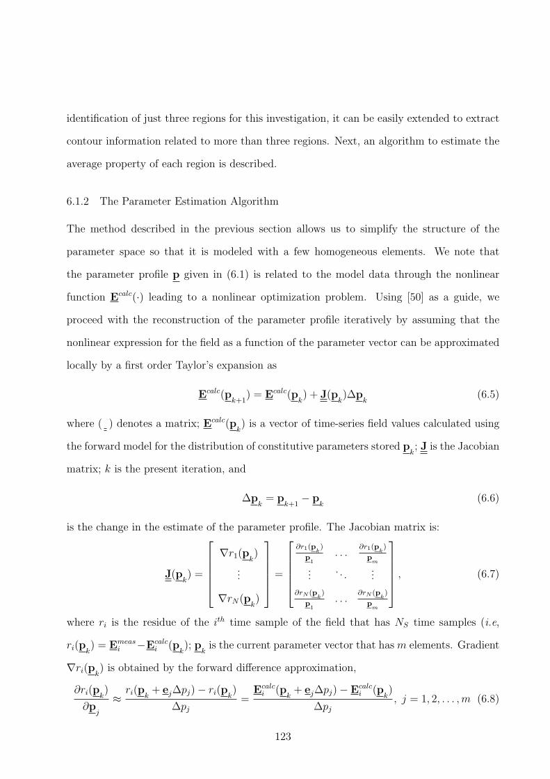
identification of just three regions for this investigation, it can be easily extended to extract
contour information related to more than three regions. Next, an algorithm to estimate the
average property of each region is described.
6.1.2 The Parameter Estimation Algorithm
The method described in the previous section allows us to simplify the structure of the
parameter space so that it is modeled with a few homogeneous elements. We note that
the parameter profile p given in (6.1) is related to the model data through the nonlinear
function Ecalc(·) leading to a nonlinear optimization problem. Using [50] as a guide, we
proceed with the reconstruction of the parameter profile iteratively by assuming that the
nonlinear expression for the field as a function of the parameter vector can be approximated
locally by a first order Taylor’s expansion as
Ecalc(pk+1
) = Ecalc(pk) + J(p
k)∆p
k(6.5)
where ( ) denotes a matrix; Ecalc(pk) is a vector of time-series field values calculated using
the forward model for the distribution of constitutive parameters stored pk; J is the Jacobian
matrix; k is the present iteration, and
∆pk
= pk+1
− pk
(6.6)
is the change in the estimate of the parameter profile. The Jacobian matrix is:
J(pk) =
∇r1(pk)
...
∇rN(pk)
=
∂r1(pk)
p1
. . .∂r1(p
k)
pm
.... . .
...
∂rN (pk)
p1
. . .∂rN (p
k)
pm
, (6.7)
where ri is the residue of the ith time sample of the field that has NS time samples (i.e,
ri(pk) = Emeas
i −Ecalci (p
k); p
kis the current parameter vector that has m elements. Gradient
∇ri(pk) is obtained by the forward difference approximation,
∂ri(pk)
∂pj
≈ri(pk
+ ej∆pj) − ri(pk)
∆pj
=Ecalc
i (pk+ ej∆pj) − Ecalc
i (pk)
∆pj
, j = 1, 2, . . . ,m (6.8)
123

where ej = [0, . . . , 1, 0, . . . , 0] is the unit vector of the jth coordinate; ∆pj is a scalar rep-
resenting the incremental change of the jth component of the parameter vector. That is,
the parameter profile pj
is perturbed by ej∆pj and the forward solver is run to calculate
Ecalci (p
k+ ej∆pj). Substituting (6.5) into (6.1) leads to the local linear objective function
F (∆pk) =
∥∥∥J∆pk+ rk
∥∥∥2
2(6.9)
which is a quadratic function of ∆pk, so
F (∆pk) = ∆pT
kJTJ∆p
k+ 2rT
k J∆pk+ rT
k rk (6.10)
where rk = Ecalc(pk) − Emeas (i.e., the residue or discrepancy between the modeled and
measured electric field data). Since F is a quadratic function of ∆pk, the change in parameter
profile ∆pk
that minimizes F is solved by determining the point where the gradient vanishes
which yields
JTJ∆pk
= −JT rk. (6.11)
Approximating the objective function locally with a linear function and the iterative method-
ology used to find its minimizer are also used by other MW breast-imaging time and fre-
quency domain tomographic approaches (cf [68] and [28], respectively) to solve the nonlinear
problem.
On many occasions, the values associated with the relative permittivity parameters are
several orders of magnitude greater than the values associated with the conductivity param-
eters. This results in what is referred to as a poorly scaled objective function [53] where
changes in one independent variable lead to much larger variations in the objective function
than changes in another. This leads to poor reconstruction results as rapid changes in the ob-
jective function along certain directions cause the local function to be a poor approximation
along these directions (cf [68] and [48] for a description of how the difference in magnitude
between the relative permittivity and conductivity parameters affects the reconstruction re-
sults for time and frequency domain approaches, respectively). The methodology proposed
124

in this Chapter to remedy this problem differs from various approaches adopted by other
MW breast imaging techniques.
If we have a priori information about the expected range of the values for pk, then we
can perform a change of variables suggested by [53] to transform the problem so that all of
the parameters have approximately the same relative accuracy. We extend this basic idea
to our nonlinear problem by first making the change of parameters
∆pk
= D∆pk
(6.12)
where D is a diagonal scaling matrix that is invertible and transforms ∆pk
to ∆pk
such that
∆pk≈ [1...1 1...1]T . Since D is invertible
∆pk
= D−1∆pk. (6.13)
The key idea of the scaling method presented in this Chapter is that when (6.13) is substi-
tuted into (6.10), the result is a rescaled local linear function F expressed in terms of the
transformed parameters
F (∆pk) = F (D−1∆p
k) = F (∆p
k) (6.14)
= ∆pT
kD−1JTJD−1∆p
k+ 2rT
k JD−1∆pk+ rT
k rk. (6.15)
The rescaled function is now equally sensitive to changes to any independent variable which
improves its accuracy in the local region of the objective function. Furthermore, the intro-
duction of the transformed parameters also yields a rescaled gradient
∂F (∆pk)
∂∆pk
= 2D−1JTJD−1∆pk+ 2D−1JT rk. (6.16)
Setting the rescaled gradient to zero results in
D−1JTJD−1∆pk
= −D−1JT rk (6.17)
which is used to solve for ∆pk. The scaling (or transforming) matrix is then used to recover
the solution (∆pk) to the original unscaled problem from ∆p
kusing (6.13).
125

This approach of rescaling the parameters to transform the objective function is different
than the Jacobian weighting scheme suggested in [48]. For the Jacobian weighting scheme, a
weighting factor is multiplied with various submatrices of the Jacobian matrix and the trans-
pose of the Jacobian matrix. Conversely, the rescaling procedure proposed in this Chapter
requires the straightforward formulation of a single component, namely the scaling matrix.
Hence, this approach is much simpler and intuitive compared to the Jacobian weighting
scheme. A simple, intuitive technique is highly beneficial in complex scenario such as MW
breast imaging.
We are presently using the Levenberg-Marquardt (LM) method to update the change
in parameter profile for the iterative parameter profile reconstruction problem. Hence, the
solution evaluated using (6.17) is stabilized by augmenting the scaled matrix, D−1JTJD−1,
that approximates the Hessian matrix on the left-hand-side of (6.17) with an additional term
leading to
(D−1JTJD−1 + λLMDLM
)∆pk
= −D−1JT rk (6.18)
where DLM
is the diagonal of D−1JTJD−1, and λLM is the LM parameter. The LM parame-
ter is determined as the iteration progresses by following a trust-region paradigm in which the
method will only trust the local linear model within a limited neighborhood (or trust-region)
of the point pk. This serves to limit the step size ∆p
k. The strategy for selecting the value of
λLM , which controls the radius of the trust region, is based on how accurately the local linear
function approximates the objective function. More specifically, the expansion/contraction
of the trust region radius (and hence the step size) and the acceptance/rejection of the new
approximation pk+1
is determined by comparing the actual reduction in the objective func-
tion using pk+1
with the predicted reduction (i.e., the decrease in the local linear function).
Refer to [50] or [53] for further details. Since the modified Hessian matrix in the left-hand side
of (6.18) is positive definite, we solve for ∆pk
using Cholesky factorization. The parameter
126

profile is updated with
pk+1
= pk+ D−1∆p
k. (6.19)
We refer to (6.14) - (6.19) collectively as the iterative nonlinear parameter estimation algo-
rithm.
The optimization technique used by this algorithm is referred to as a second order method
and finds the minimizer in a fast and efficient manner (i.e., fewer iterations are required due
to the superior convergence behavior of the method compared to gradient approaches (cf
[53])). It differs from other reported breast imaging time-domain approaches (see [70]- [68]
for examples) which estimate a very large number of parameters and uses gradient-based
approaches to find the minimizer.
6.1.3 Integrating radar and tomography
We observe that (5.3) implies that the value of each point estimated on the contour Γ23 de-
pends on the value ǫr2. Moreover, the regional geometric properties depend on ǫr2 since the
contour model is constructed from these points. We exploit this dependence in order to incor-
porate the reconstruction model into the parameter estimation algorithm. The methodology
used to achieve this starts with the formulation of a univariant objective function described
next.
First, we consider the scenario where the value of ǫr2 is fixed and deterministic. Since
points estimated on contour Γ23 depend on ǫr2, fixing the value of ǫr2 also determines the
geometric models formed by the reconstruction model estimation algorithm. This determin-
istic view of ǫr2 allows us to evaluate dielectric property estimates for regions 1 and 3 over
the reconstruction model using the objective function given by
F (p23
; ǫr2) =∥∥∥Ecalc(p
23; ǫr2) − Emeas
∥∥∥2
2(6.20)
where p23
= [ǫr1 ǫr3 σ1 σ2 σ3]T . The cost functional is parameterized by ǫr2, i.e., we have a
class of cost functionals where each one is different due to a different value of ǫr2. We use a
127

Figure 6.3: The radar-based techniques use laser data and reflection data (dashed boxes) toform a reconstruction model. For each iteration, MWT is applied to Tx/Rx data to estimatethe dielectric properties of the model (gray box). The golden section algorithm integrates thetwo methods to iteratively estimate the mean dielectric properties over each region (loop).
128

Figure 6.4: Interval of uncertainty [ǫr2,min, ǫr2,max] with increasing iterations represented asblue and black dot, respectively. The golden section algorithm selects these points (reddot) from the interval such that the interval of uncertainty containing the minimizer isprogressively reduced until the minimizer is ’boxed in’ with sufficient accuracy.
semicolon to denote this dependence since the value of ǫr2 affects the cost functional of p23
.
Our goal is to find the minimizer of (6.20) over the closed interval [ǫr2,min, ǫr2,max]. Since
(6.20) is univariant, we use the 1D golden section search approach to find the minimizer (cf
[51] for a detailed description of this algorithm).
The method is summarized in Fig. 6.3. First, the parameter vector p23
is initialized
with average literature values (e.g., [12]). Second, the reconstruction model is assembled.
By assumption, the outer surface estimate Γ01 is known a priori. To define the skin layer,
the initial value of the skin permittivity is combined with the information from the RDD
algorithm, and (5.3) is used to estimate the average skin thickness w1,avg. Surface contour
Γ01 is offset by w1,avg to form an estimate of Γ12.
Next, the regions inside the skin dominated by fat and glandular tissue are defined. A
bracketing method (cf [122]) defines a closed interval referred to as the interval of uncer-
tainty that contains the minimizer of (6.20). The algorithm selects an initial value for ǫr2
from this interval. As described in Section 6.1.1, reflection data from N antennas are used
with the initial value for ǫr2 to identify the sequence of points to construct contour Γ23.
129

Estimates of contours Γ01, Γ12, and Γ23 identify regions Σ1, Σ2, and Σ3 to collectively form
the reconstruction model as described in Section 6.1.1.
With the formation of the reconstruction model complete, the parameter space is parti-
tioned into three disjoint regions and the MWT method described in Section 6.1.2 is applied
to the transmission/reflection data to evaluate p23
for the given value of ǫr2 that minimizes
(6.20). The golden section method uses the resulting value of F (p23
; ǫr2) to narrow the
interval of uncertainty which completes an iteration of the algorithm.
The procedure is repeated for further iterations to minimize the objective function given
by (6.20) at different points in [ǫr2,min, ǫr2,max]. This is demonstrated by the example in
Fig. 6.4 where ǫr2,min and ǫr2,max are represented by the blue and black dot, respectively. The
golden section algorithm selects these points (the red dot in Fig. 6.4) so that the interval of
uncertainty containing the minimizer is progressively reduced until the minimizer is ’boxed
in’ with sufficient accuracy. By using this strategy we have reduced a multi-dimensional
optimization problem to a univariant optimization problem. Furthermore, since the function
is evaluated over an interval of values, the risk of getting trapped in a false solution is reduced.
We note that when applying the golden section procedure, for each ǫr2 selected from the
interval of uncertainty, the reconstruction model is evaluated from reflection data prior to
calling the MWT algorithm. The motivation for integrating the radar-based methods with
MWT is to extract information from the reflection data corresponding to the internal struc-
ture of the breast. Knowledge of this internal structural information is used to help alleviate
the ill-posedness of the inverse scattering problem. Furthermore, the radar-based technique
forms a reconstruction model consisting of regions separated with sharp interfaces (i.e., there
is not a gradual transition from one region to another). This allows the contours separat-
ing regions to be preserved in the reconstruction process. Based on the methodology used
to build the reconstruction model (i.e., using homogeneous model elements whose shapes
are extracted from UWB reflection data), the physical interpretation of the reconstruction
130

Table 6.1: Dielectric properties of the three regions used by the models 1 and 2 [12, 143].
Tissue Type ǫr σImmersion medium 1.0 0.0Region 1 (skin) 36.0 4.0Region 2 (adipose) 9.0 0.4Region 3 - fibroglandular 1 15.2 1.7Region 3 - fibroglandular 2 27.2 3.0Region 3 - fibroglandular 3 40.0 3.2Region 3 - Tumor 50.0 4.0
profiles corresponds to spatial averages of the parameters.
6.2 Initial algorithm performance evaluation
The ability of the algorithm to evaluate regional geometric and dielectric properties of an
object is first evaluated with a 2D object having progressively more complex regional shapes
and distributions. The approach used to generate the numerical data and the metrics used
to evaluate the performance of the algorithm are described in Section 6.2.1 and Section 6.2.2,
respectively. The results and performance of the algorithm are described in Section 6.2.3.
6.2.1 Generation of Numerical Data
Numerical simulations with the FDTD method are used to generate test data. In these
examples, the FDTD problem space is bounded by a five-cell thick perfectly matched layer
(PML) boundary layer (4th order, R(0) = 10−7) with spatial grid resolution of 1.0 mm.
Similar to the illustration in Fig. 6.2, a model having three distinct regions is placed within
the problem space. For this study, free space is used for the measurement region. The
dielectric properties of each region used by the model are shown in Table 6.1. Random
perturbations of ±10% around the dielectric property values for each region are introduced.
The standard deviation of the relative permittivity of region 3 for the ith model is calculated
131

with
std(ǫr3)i =
√√√√ 1
Nr3
Nr3∑
p=1
(ǫr3,p − ǫr3) (6.21)
where Nr3 is the total number of model elements (or pixels) in the electromagnetic model
in region 3; and ǫr3,p is the relative permittivity of the pth model element in region 3. The
mean value of the relative permittivity over region 3 of the model used in (6.21) is
ǫr3 =1
Nr3
Nr3∑
p=1
ǫr3,p. (6.22)
The standard deviation of the relative permittivity of region 3 for each model is normalized
to the standard deviation of region 3 for model 1. That is,
V ar(ǫr3)i =std(ǫr3)i
std(ǫr3)1
, (6.23)
which means that V ar(ǫr3)i is a metric that provides a measure of the variability of the
relative permittivity within region 3 for the ith model.
Two approaches are used to collect data for the contour sample evaluation and parameter
estimation algorithms.
Evaluating contour samples from Rx data
To evaluate the contour samples, a reflection configuration consists of a co-located source
and sensor on the boundary ∂Ω of the region of interest and 10 mm from the surface of the
model. The source is modeled as an impressed current source in these TMx simulations. A
pulse is used for the time-domain excitation function
S(t) = s0(t− t0) exp(−(t− t0)2/τ 2) (6.24)
where s0 is a scalar, t0 is the centre of the pulse in time, and τ is a variable that controls
the rise time of the pulse. The value of τ is adjusted so that the pulse has the required
maximum frequency, fmax, content. Here, fmax, is the frequency of the spectrum where the
magnitude of S(ω) is 10% of its maximum magnitude. Simulations are performed with
132

fmax = 8.92 GHz. In all of the examples, the number of samples is NS = 4000 and the
sample time is Ts = 2.12 ps. Reflections are recorded as the sensor is scanned to 40 equally
spaced locations around the model. Data received by the sensor are conditioned such that
the transmitted signal is removed from each reflection. The transmitted signal is acquired
by carrying out a simulation without the model. The data are finally normalized to the
reflected signal’s maximum positive value and are contaminated with samples generated by
a zero-mean Gaussian white noise process such that a signal-to-noise ratio (SNR) of 25 dB
is attained. The SNR is defined as the ratio of the signal energy to total noise energy, so a
SNR of 25 means that the signal energy is 25 dB above the total noise energy.
When estimating the TOA parameter from the reflections, reference signals are required
as indicated in Chapter 5. For all of the examples, the reference signals are acquired by
simulating a homogeneous planar layer (slab) having dielectric properties of ǫr = 37.5, σ =
4.2 S/m. The reflection from the slab is normalized and used for the first reference signal
r1(t). To acquire the second reference signal, r2(t), a simulation is carried out with a 2 layer
slab. A 3 mm thick outer layer has the same properties as the slab used to acquire the first
reference signal and a second layer has dielectric properties of ǫr = 9.0, σ = 0.4 S/m. The
reflection from the first interface, r1(t), is subtracted from the resulting reflection in order
to isolate the reflection from the second interface. The subtracted signal is then normalized
to the first reference signal and used as the second reference signal, r2(t). Finally, we use
the first reference signal for r3(t). We justify using two different reference signals since the
breast skin thickness is typically between 0.7 and 2.3 mm [134].
Parameter estimation from transmission/reflection data
A second configuration is used to collect data for parameter estimation, which we refer to as
the transmission-reflection configuration. This consists of a source and two sensors located on
the boundary ∂Ω of the region of interest and located 10 mm from the surface of the model.
One sensor is located at the same location as the source to record reflection data and the
133

Figure 6.5: The shared area is the intersection of the actual and estimated regions. The errorarea is the area in an actual and estimated region not shared by both regions and representsthe discrepancy between the estimated and actual geometric models. The error ratio is theratio between the error and shared areas.
second sensor is located directly opposite the source to collect transmission data. Simulations
are performed with fmax = 4.83 GHz. This maximum frequency, fmax, is lower compared to
the fmax of the incident field used for collecting the reflection data (where, fmax = 8.92 GHz ).
For the tomography approach, the incident field must propagate across the diameter of the
breast. An incident field with a lower spectral content is used to reduce the losses that occur
over the required distance. A complete set of data is collected by moving the source and
sensors sequentially to 4, 8 or 16 equally spaced locations on the boundary. We note that
this approach to data collection is different from traditional tomographic data collection
approaches indicated in [55] - [76], where an antenna illuminates the object and several
antennas are positioned around the boundary to record the scattered fields. Each signal
(consisting of a time-series of electric field values) recorded by a receiver is contaminated
with noise samples derived from a zero-mean white Gaussian noise process such that a SNR
of 25 dB is attained. The noisy signals simulate the time-series measured data, Emeas, and
are used by the iterative nonlinear parameter estimation algorithm to estimate the regional
dielectric properties using the procedure depicted in Fig. 6.3.
134
Figure 6.6: Model 1 relative permittivity profile (left) and contour samples (dots) evaluatedfor contour Γ23 (right). The ith contour sample PΓ23(i) is evaluated from the reflection datay(t) recorded by the ith sensor (rectangle) with the procedure described in Section 6.1.1which uses the line-of-sight rays shown connecting each sensor with the center of the model.
6.2.2 Assessing the performance of the algorithm
Three quantitative measures are used to evaluate the quality of the parameter reconstruction
results. The ability of the algorithm to accurately estimate the mean dielectric properties in
each region is evaluated by computing the relative error of the parameter:
relative error =µj − µj
µj
× 100% for j = 1, 2, or 3 (6.25)
where µj is the spatial mean value of the estimated parameter evaluated over the estimate
of the jth region Σj ; and µj is the actual spatial mean of the parameter evaluated over this
same region.
The normalized root mean square error (NRMSE) measures the discrepancy between the
actual and reconstructed parameter profiles. The discrepancy is also called the residue so
this measure implies the precision of the estimation technique. The measure is normalized
by the range of actual profile values and is given by
NRMSE(p, p) =1
pmax − pmin
√∑ni=1(pi − pi)2
n(6.26)
135

Table 6.2: Regional dielectric parameter estimation results for model 1 using a transmis-sion-reflection configuration with a varying number of sensors.
4 sensor 8 sensor 16 sensor
Rel. err. Rel. err. Rel. err.Actual Est. (%) Actual Est. (%) Actual Est. (%)
ǫr1 35.89 37.19 3.63 35.89 35.74 -0.40 35.89 36.96 2.98σ1 4.01 3.77 -6.08 4.01 4.06 1.17 4.01 3.75 -6.50ǫr2 9.16 10.12 10.47 9.75 8.81 9.62 9.13 10.16 11.38σ2 0.41 0.45 8.80 0.47 0.40 14.97 0.41 0.45 8.97ǫr3 36.72 32.39 -11.78 38.12 37.94 0.47 36.61 36.46 -0.41σ3 2.91 2.89 -0.59 3.04 2.96 2.72 2.90 2.78 -4.12
where n is the length of the vectorized parametric profile; pmax and pmin are the maximum
and minimum values of the actual profile, respectively; pi and pi are elements in the actual
and estimated profiles, respectively. The value is expressed as a percentage where a lower
value indicates less residual variance.
A metric referred to as the error ratio is illustrated in Fig. 6.5 and provides a quantitative
measure of the ability of the algorithms to accurately model the contour and the regional
geometrical properties. First, a selected region is identified based on the property profile,
while the estimated regions are those created using the procedure described in Section 6.1.1.
The intersection of the actual and estimated regions is referred to as the shared area. The
area in an actual or estimated region that is not shared by both regions is referred to as the
error area which means that the error area represents the discrepancy between the estimated
and actual geometrical models. Finally, the error ratio is the ratio between the error area
and the shared area. The error and shared areas are also imaged to form an error map to
visually represent the discrepancy between the modeled and actual regions.
6.2.3 Results
We first evaluate the feasibility of the proposed approach for a simple case whereby the three
regions are each relatively homogeneous and are well segregated from each other. The results
136
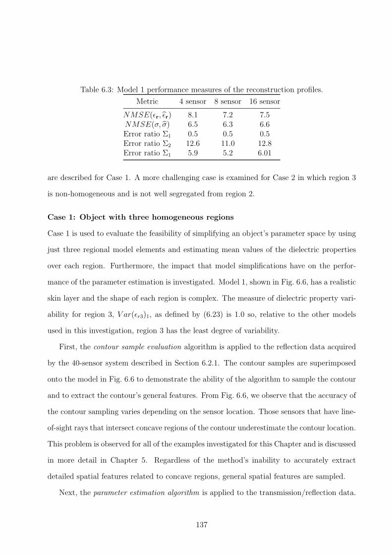
Table 6.3: Model 1 performance measures of the reconstruction profiles.
Metric 4 sensor 8 sensor 16 sensor
NMSE(ǫr, ǫr) 8.1 7.2 7.5NMSE(σ, σ) 6.5 6.3 6.6Error ratio Σ1 0.5 0.5 0.5Error ratio Σ2 12.6 11.0 12.8Error ratio Σ1 5.9 5.2 6.01
are described for Case 1. A more challenging case is examined for Case 2 in which region 3
is non-homogeneous and is not well segregated from region 2.
Case 1: Object with three homogeneous regions
Case 1 is used to evaluate the feasibility of simplifying an object’s parameter space by using
just three regional model elements and estimating mean values of the dielectric properties
over each region. Furthermore, the impact that model simplifications have on the perfor-
mance of the parameter estimation is investigated. Model 1, shown in Fig. 6.6, has a realistic
skin layer and the shape of each region is complex. The measure of dielectric property vari-
ability for region 3, V ar(ǫr3)1, as defined by (6.23) is 1.0 so, relative to the other models
used in this investigation, region 3 has the least degree of variability.
First, the contour sample evaluation algorithm is applied to the reflection data acquired
by the 40-sensor system described in Section 6.2.1. The contour samples are superimposed
onto the model in Fig. 6.6 to demonstrate the ability of the algorithm to sample the contour
and to extract the contour’s general features. From Fig. 6.6, we observe that the accuracy of
the contour sampling varies depending on the sensor location. Those sensors that have line-
of-sight rays that intersect concave regions of the contour underestimate the contour location.
This problem is observed for all of the examples investigated for this Chapter and is discussed
in more detail in Chapter 5. Regardless of the method’s inability to accurately extract
detailed spatial features related to concave regions, general spatial features are sampled.
Next, the parameter estimation algorithm is applied to the transmission/reflection data.
137

z (mm)
y (m
m)
20 40 60 80 100 120 140 160
20
40
60
80
100
120
140
160
5
10
15
20
25
30
35
40
εr
z (mm)y
(mm
)
20 40 60 80 100 120 140 160
20
40
60
80
100
120
140
160
5
10
15
20
25
30
35
40
εr
z (mm)
y (m
m)
20 40 60 80 100 120 140 160
20
40
60
80
100
120
140
160
1.5
2
2.5
3
3.5
4
σ
z (mm)
y (m
m)
20 40 60 80 100 120 140 160
20
40
60
80
100
120
140
160
1.5
2
2.5
3
3.5
4
σ
Figure 6.7: Model 1 reconstruction results. Actual and reconstructed profiles of the relativepermittivity are shown on the top left and right, respectively. Actual and reconstructedprofiles of the conductivity are shown on the bottom left and right, respectively.
When constructing the regional skin model for the first iteration of the parameter estimation
algorithm, a value of ǫr = 36.0 σ = 4.0 S/m is used in (5.3) to evaluate the estimated mean
skin thickness. Thereafter, the mean thickness for the present iteration is evaluated using
the dielectric property estimates from the previous iteration. This approach is used for all
examples presented. The actual skin thickness varies from 1.71 mm to 2.44 mm and the
mean value is 2.11 mm; the estimated mean skin thickness is 2.13 mm. Since the spatial grid
resolution is 1 mm, the surface contour Γ01 is offset by 2 mm to estimate Γ12 and hence to
construct the skin region model. The golden section algorithm typically converges after 12-14
138

iterations for all of the examples studied. For the 8 sensor system, estimating the regional
properties typically takes about 1 min/iteration (30 sec/iteration and 2 min/iteration for 4
and 16 sensor systems, respectively).
Figure 6.7 shows the reconstructed profiles, while Table 6.2 summarizes the parameter
estimation results using the relative error as the performance metric and Table 6.3 presents
the remaining error metrics. Overall, the algorithm estimates the mean dielectric properties
for the skin and fibroglandular (region 3) regions very accurately. The values of the error
ratio shown in Table 6.3 for these regions also suggest that accurate regional modeling is
achieved. Region 2 has a larger error ratio than the other regions and the relative error
of the dielectric parameters for region 2 is correspondingly greater. However, this error is
less than 15% for both parameters. Moreover, the discrepancy measures suggest that both
the conductivity and relative permittivity profiles of the object are reconstructed accurately.
Finally, for this model, it appears that increasing the number of sensors marginally improves
the parameter estimation results.
Two sources that contribute to model errors are: dielectric property errors that arise
by modeling a heterogeneous region with a homogeneous model element; and geometric
property errors that arise due to inaccuracies of the contour model. The geometric errors
between the regional model element and the actual region are examined more closely in the
error map shown in Fig. 6.8. For region 2, the error map shown in Fig. 6.8 suggests that
the error area is dominated by material that should be modeled as part of region 2 but is
mistakenly represented as part of region 3. This means that the model errors that may bias
the estimated dielectric parameter values are primarily due to geometrical discrepancies.
Conversely, the error map for region 3 suggests that the regional model element mistakenly
contains a mix of material from regions 2 and 3 which means that the model element no
longer represents a homogeneous region. Therefore, both geometric and dielectric property
model errors are introduced which may collectively impact the accuracy of the dielectric
139

Table 6.4: Comparison of regional dielectric parameter estimation results for model 1 using8 sensor Tx/Rx configuration with varying SNR (both WGN and colored). The dielectricparameter results are expressed in terms of relative error (%).
25 dB 20 dB 10 dB
WGN Colored WGN Colored WGN Colored
ǫr1 -0.40 1.89 0.54 -2.27 1.39 -0.67σ1 1.17 -1.63 5.70 7.86 11.35 9.84ǫr2 9.62 2.00 -9.99 -2.21 -14.33 -15.88σ2 14.97 -1.58 -5.09 -3.50 -15.21 -15.56ǫr3 0.47 -9.28 2.70 4.66 13.53 12.23σ3 2.72 -5.10 -9.42 3.43 -23.03 -6.58
Error ratio Σ1 0.5 0.5 0.5 0.5 0.5 0.5Error ratio Σ2 7.10 5.04 6.64 5.20 6.94 7.37Error ratio Σ1 15.14 10.74 14.15 11.09 14.80 15.70
property estimates for this region.
Next the effect of low SNR conditions and the presence of colored noise samples are
investigated with an 8 sensor MWT system. The samples from the colored noise process are
obtained by filtering a Gaussian process. The results are shown in Table 6.4. We observe
that the quality of the regional estimates for the adipose region start to deteriorate for noise
levels of 20 dB, although the relative error of the estimates is still below 15 % for an SNR of
20 dB for both white and colored noise. As expected, the overall quality of the estimates is
worse when the signals are contaminated with colored noise compared to the case when the
signals are contaminated with white noise. When using a least squares estimator, we assume
that the noise samples contaminating the signal have a mean of zero and are uncorrelated
[124].
Significantly, Table 6.4 also shows that there is only a marginal increase in geometrical
model errors as the SNR decreases. That is, there is not as significant deterioration in the
accuracy of the regional geometric properties compared to the regional dielectric properties,
implying that estimation of the geometric properties is much more robust to the presence
of noise (both white and colored) compared to the regional dielectric property estimation.
140

Table 6.5: Comparison of regional dielectric parameter estimation results for model 1 usingtraditional MWT configuration with varying number of sensors.
4 sensor 8 sensor 16 sensor
Rel. err. Rel. err. Rel. err.Actual Est. (%) Actual Est. (%) Actual Est. (%)
ǫr1 35.89 35.98 0.27 35.89 35.85 -0.09 35.89 35.91 0.06σ1 4.01 4.02 0.25 4.01 3.97 -1.16 4.01 3.97 -1.12ǫr2 9.72 8.95 -7.99 9.49 9.16 -3.49 9.49 9.16 -3.49σ2 0.47 0.40 -14.56 0.44 0.41 -8.31 0.44 0.41 -8.31ǫr3 37.98 36.18 -4.74 37.71 37.04 -1.77 37.71 37.27 -1.18σ3 3.02 3.06 1.20 3.00 2.93 -2.20 3.00 2.96 -1.51
This result highlights an advantage of integrating radar-based techniques with MWT. We
attribute this robustness to the fact that the contour samples are estimated using the RDD al-
gorithm which is robust to the presence of both colored and white noise at low signal-to-noise
levels as demonstrated in Chapter 5. The algorithm is able to resolve the interface between
regions, so it provides a means of preserving the imaging resolution at low signal-to-noise
levels. For typical MWT methods, an increase in SNR leads to a shift and disappearance of
the fibroglandular region compared to the noiseless case (e.g., [27]).
We have already noted that the approach used for collecting reflection/transmission data
described in Section 6.2.1 is different from traditional MWT data collection approaches,
where an antenna illuminates the object and several antennas are positioned around the
boundary to record the scattered fields. We repeat the parameter estimation procedure using
the traditional MWT data collection approach to determine if there is an improvement in
the accuracy of the dielectric property estimates. A traditional MWT system is one in which
a target is encircled by an array of antennas. The target is then illuminated sequentially
by each antenna, while the remaining antennas record the scattered fields. The process
continues until all antennas have acted as a transmitter. The results are shown in Table
6.5, indicating an improvement in the accuracy of the estimates compared to the results
shown in Table 6.2; but the improvement is not significant. We conjecture that the use
141

z (mm)
y (m
m)
20 40 60 80 100 120 140 160
20
40
60
80
100
120
140
160
z (mm)
y (m
m)
20 40 60 80 100 120 140 160
20
40
60
80
100
120
140
160
Figure 6.8: Model 1 error maps for region 2 (left) and region 3 (right). Shared area whereestimated and actual geometrical models match displayed as light blue. Yellow shows whereregion 2 is mistakenly modeled as part of region 3. Where region 3 mistakenly containsregion 2 material is shown in red and error area where material that should be part of region3 is mistakenly modeled as part of region 2 shown in yellow.
of reflection data by the radar-based technique incorporates a priori information about
the internal breast structure into the inversion process. Therefore, although the traditional
MWT data collection approach provides an increase in the number of views examined for each
illumination, the observation suggests that there is not a significant increase in the amount
of additional information extracted from the signals compared to the Tx/Rx configuration.
Regardless of the presence of geometric and dielectric model errors, these initial results
demonstrate that the algorithm is able to accurately characterize the very complicated in-
terfaces between the different regions. This is achieved due to the preservation of the sharp
interfaces between regions which allows accurate identification of the regions that describe
the general internal structure of a dielectric object. The results support the basic idea of sim-
plifying an object’s parameter space by identifying the predominate regions and then using
just a few regional model elements. Once these regions are identified, the algorithm is able
to accurately estimate the mean dielectric properties over each region in spite of the complex
spatial features. Although errors exist using these model simplifications, the algorithm is
142

Figure 6.9: Model 2 actual and reconstructed profiles of relative permittivity shown on topleft and right, respectively. Contour samples (dots) evaluated for Γ23(bottom).
robust to the impact they have on the performance of the estimation procedure and also to
the presence of noise. This case demonstrates the successful integration of techniques used
to extract information from both reflection and transmission data to provide information
about the internal structure of an object.
Case 2: Object with complex parameter profile for region 3
The second model is used to evaluate the effect of modeling a heterogeneous region with a
homogeneous model element. The model shown in Fig. 6.9 has a more complicated region
3 compared to the first model examined; region 3 is heterogeneous and it is not possible
to segregate regions 2 and 3. This leads to the existence of isolated scatterers. Material
143

Table 6.6: Regional dielectric parameter estimation results for models 2 - 4 using 16 sensortransmission-reflection configuration.
Model 2 Model 3 Model 4
Rel. err. Rel. err. Rel. err.Actual Est. (%) Actual Est. (%) Actual Est. (%)
ǫr1 35.88 36.65 2.14 36.05 36.90 2.36 36.17 34.07 -5.80σ1 4.00 3.79 -5.25 4.01 4.10 2.25 3.99 4.25 6.71ǫr2 9.14 10.02 9.59 10.18 8.63 -15.29 11.34 8.82 -22.22σ2 0.41 0.43 5.55 0.47 0.38 -17.76 0.59 0.39 -33.68ǫr3 28.12 24.61 -12.50 25.16 25.90 2.93 28.92 27.60 -4.57σ3 2.35 2.32 -1.29 2.20 2.39 8.42 2.51 2.35 -6.34
with ǫr = 50 is mixed in with material with ǫr = 15.2 so there is a great deal of dielectric
property variation within region 3. The measure of dielectric property variability for region
3, V ar(ǫr3)2, as defined by (6.23) is 3.4. Therefore, this model permits investigation of the
effectiveness of the modeling technique to estimate the average properties of a heterogeneous
region.
The contour sample evaluation algorithm is applied to the reflection data acquired by the
40-sensor system and the contour samples are superimposed onto the model in Fig. 6.9. From
Fig. 6.9, we observe that the contour samples provide a general outline of region 3 indicating
that general features are extracted despite the complex shape. However, the contour sample
technique does not identify individual region 3 scatterers, i.e., the outline of region 3 formed
by the contour samples includes material from both regions 2 and 3 which further increases
the variability and the degree of heterogeneity of the properties within region 3. As in the
previous case, the actual mean thickness of the skin is 2.11 mm and the estimated mean skin
thickness is 2.13 mm.
Next, the parameter estimation algorithm is applied to the transmission/reflection data
collected by moving the source and sensors sequentially to 16 equally spaced locations on
the boundary. Figure 6.9 shows the reconstructed relative permittivity profile, while Ta-
ble 6.6 summarizes the parameter estimation results obtained for the data collection system.
144
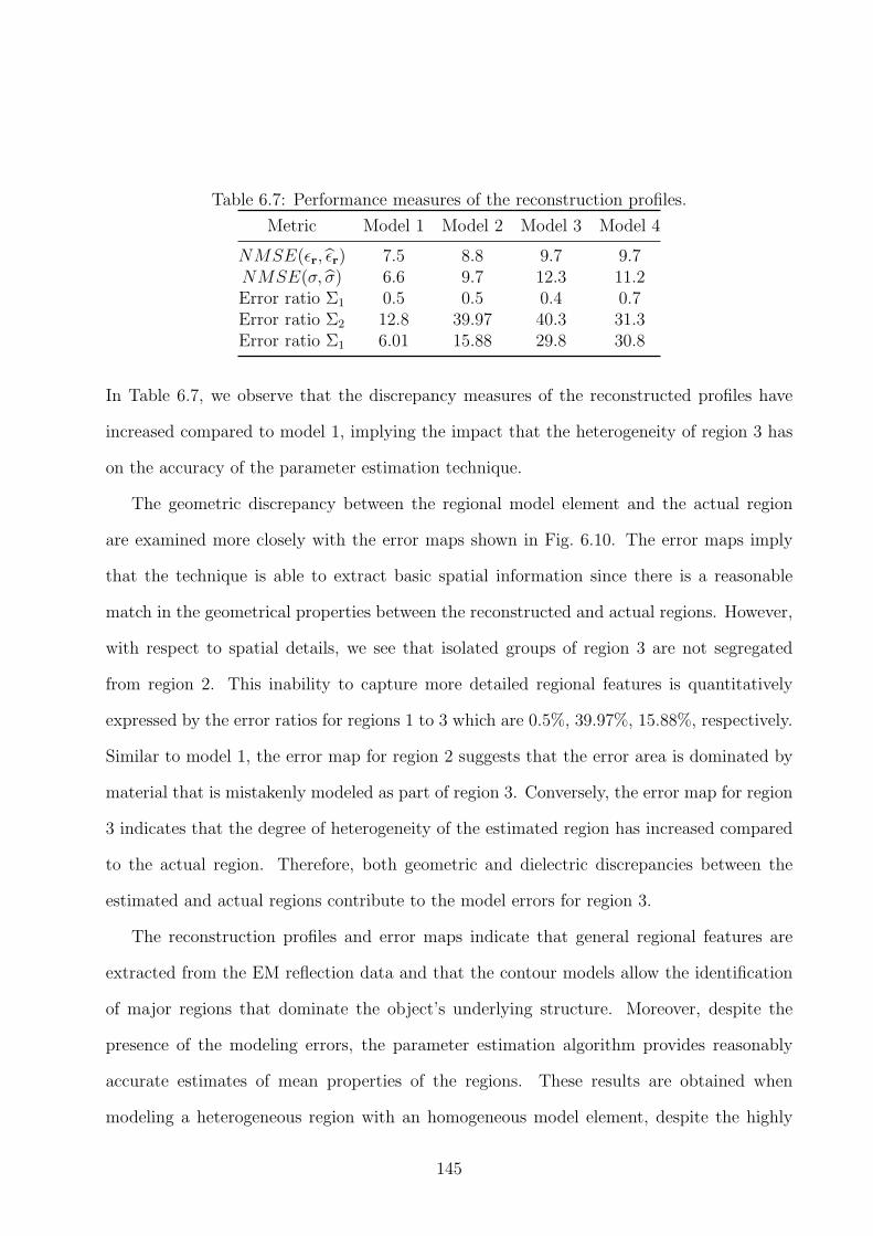
Table 6.7: Performance measures of the reconstruction profiles.
Metric Model 1 Model 2 Model 3 Model 4
NMSE(ǫr, ǫr) 7.5 8.8 9.7 9.7NMSE(σ, σ) 6.6 9.7 12.3 11.2Error ratio Σ1 0.5 0.5 0.4 0.7Error ratio Σ2 12.8 39.97 40.3 31.3Error ratio Σ1 6.01 15.88 29.8 30.8
In Table 6.7, we observe that the discrepancy measures of the reconstructed profiles have
increased compared to model 1, implying the impact that the heterogeneity of region 3 has
on the accuracy of the parameter estimation technique.
The geometric discrepancy between the regional model element and the actual region
are examined more closely with the error maps shown in Fig. 6.10. The error maps imply
that the technique is able to extract basic spatial information since there is a reasonable
match in the geometrical properties between the reconstructed and actual regions. However,
with respect to spatial details, we see that isolated groups of region 3 are not segregated
from region 2. This inability to capture more detailed regional features is quantitatively
expressed by the error ratios for regions 1 to 3 which are 0.5%, 39.97%, 15.88%, respectively.
Similar to model 1, the error map for region 2 suggests that the error area is dominated by
material that is mistakenly modeled as part of region 3. Conversely, the error map for region
3 indicates that the degree of heterogeneity of the estimated region has increased compared
to the actual region. Therefore, both geometric and dielectric discrepancies between the
estimated and actual regions contribute to the model errors for region 3.
The reconstruction profiles and error maps indicate that general regional features are
extracted from the EM reflection data and that the contour models allow the identification
of major regions that dominate the object’s underlying structure. Moreover, despite the
presence of the modeling errors, the parameter estimation algorithm provides reasonably
accurate estimates of mean properties of the regions. These results are obtained when
modeling a heterogeneous region with an homogeneous model element, despite the highly
145

z (mm)
y (m
m)
20 40 60 80 100 120 140 160
20
40
60
80
100
120
140
160
z (mm)y
(mm
)
20 40 60 80 100 120 140 160
20
40
60
80
100
120
140
160
Figure 6.10: Model 2 error maps for region 2 (left) and region 3 (right). Shared area whereestimated and actual geometrical models match displayed as light blue. Region 2 error areawhere material that should be modeled as part of region 2 is mistakenly modeled as partof region 3 shown in yellow. Region 3 error area where the model for region 3 mistakenlycontains region 2 material shown in red and error area where material that should be partof region 3 is mistakenly modeled as part of region 2 shown in yellow.
heterogeneous nature and complex shape of region 3 and the presence of isolated region 3
scatterers within region 2. The results further support the feasibility of using the algorithm
to provide an object’s basic structural information in an efficient manner.
6.3 Application to a 2D numerical breast model
We now apply this technique to a practical but challenging problem in which the goal is to use
the MW data recorded by sensors to evaluate regional geometric and dielectric properties
of a breast. The accuracy and performance of the algorithm in this practical scenario is
investigated using two numerical breast models. The breast models are constructed from
coronal MR scans acquired from a patient study described in [132]. The MR scans are
collected prior to injection of a contrast agent used routinely in MR and construction of the
numerical models follows a three step procedure described in [133]. First, the breast location
is defined and a non-uniform skin layer is added. Next, the breast interior is segmented into
5 tissues. Mapping of MR pixel intensity to breast tissue electrical properties employs a
146

Figure 6.11: Model 3 actual and reconstructed profiles of relative permittivity shown on topleft and right, respectively. Contour samples (dots) evaluated for Γ23(bottom).
piecewise linear mapping by assigning ranges of pixel intensities to each of the tissue groups
defined in [12]. Model 3 contains a tumor extracted from images acquired after a contrast
agent is administered to the patient, and inserted into the numerical breast model at the
appropriate location. To further model anatomical heterogeneity of the biological tissue, we
introduce random perturbations of ±10% around the dielectric property values for the tissue
types. The relative permittivity profile of models 3 and 4 are shown in Figs. 6.11 and 6.13,
respectively, and illustrate the anatomically realistic variations of the dielectric properties
which have been derived from the MR scan. The measure of dielectric property variability
for region 3 as defined by (6.23) for models 3 and 4, relative to the first model, are V ar(ǫr3)3
147

z (mm)
y (m
m)
20 40 60 80 100 120 140 160
20
40
60
80
100
120
140
160
z (mm)y
(mm
)
20 40 60 80 100 120 140 160
20
40
60
80
100
120
140
160
Figure 6.12: Model 3 error maps for region 2 (left) and region 3 (right). Shared area whereestimated and actual geometrical models match displayed in light blue. Region 2 error areawhere adipose tissue mistakenly modeled as part of the fibroglandular region shown in yellowand the error area where fibroglandular tissue mistakenly modeled as part of the fatty regionshown in red. Region 3 error area where region 3 mistakenly contains adipose tissue shownin red and the error area where fibroglandular tissue mistakenly modeled as part of region 2shown in yellow.
= 4.2 and V ar(ǫr3)4 = 4.3, respectively.
The contour sample evaluation algorithm is applied to the reflection data acquired by
the 40 sensor system and the contour samples are superimposed onto models 3 and 4 in
Figs. 6.11 and 6.13, respectively. The actual thickness of the skin for Model 3 varies from
1.91 to 2.54 mm and the mean thickness is 2.23 mm; the estimated mean skin thickness is
2.18 mm. The actual thickness of the skin for Model 4 varies from 1.71 to 3.00 mm and
the mean thickness is 2.12 mm; the estimated mean skin thickness is 2.24 mm. We observe
that the contour samples provide a general outline of region 3 for both models, indicating
that general contour features are extracted. However, for these models, region 3 has a much
more complicated shape than the previous models studied. The many high frequency spatial
oscillations of the contour enclosing region 3 are not extracted so that it is not possible to
precisely delineate region 2 from region 3 as in previous models.
Next, the parameter estimation algorithm is applied to the transmission/reflection data
148

Figure 6.13: Model 4 actual and reconstructed profiles of relative permittivity shown on topleft and right, respectively. Contour samples (dots) evaluated for Γ23(bottom).
collected by moving the source and sensors sequentially to 16 equally spaced locations on
the boundary. The reconstructed profiles for models 3 and 4 are shown in Figs. 6.11 and
6.13, respectively. Table 6.6 summarizes the parameter estimation results obtained for the
data collection systems for these models. Similar to the first model, the algorithm appears
to provide accurate estimates of the dielectric properties for the skin and the fibroglandular
region (region 3). Table 6.7 shows the remaining performance metrics. The increase in
discrepancy compared to the same measures for model 2 imply the reduced accuracy of the
geometric and dielectric property estimates due to the elevated complexity and heterogeneity
of region 3.
149

z (mm)
y (m
m)
20 40 60 80 100 120 140 160
20
40
60
80
100
120
140
160
z (mm)y
(mm
)
20 40 60 80 100 120 140 160
20
40
60
80
100
120
140
160
Figure 6.14: Model 4 error maps for region 2 (left) and region 3 (right). Shared area whereestimated and actual geometrical models match displayed in light blue. Region 2 error areawhere adipose tissue mistakenly modeled as part of the fibroglandular region shown in yellowand the error area where fibroglandular tissue mistakenly modeled as part of the fatty regionshown in red. Region 3 error area where region 3 mistakenly contains adipose tissue shownin red and the error area where fibroglandular tissue mistakenly modeled as part of region 2shown in yellow.
The geometric discrepancy between the actual and estimated regions for model 3 is
examined more closely in the error map shown in Fig. 6.12. Although the estimate of region
2 is dominated by adipose tissue, the error map for region 2 suggests that the regional model
element mistakenly contains a mix of adipose and fibroglandular tissue (implied by the red
error area shown in Fig. 6.12) which means that this model element no longer represents
a homogeneous region. Therefore, both geometric and dielectric property model errors are
introduced which may collectively have a more significant impact on the accuracy of the
dielectric property estimates for this region compared to the first two cases. Similar to
the first two cases, the error map for region 3 suggests that adipose tissue is inadvertently
modeled with the fibroglandular tissue.
Figure 6.14 shows the error maps for model 4. Similar to model 3, the estimate of region
2 is dominated by adipose tissue, but the error map for this region suggests that a higher
proportion of fibroglandular tissue is inadvertently mixed with the adipose tissue in region 2
150

compared to model 3. This leads to larger dielectric property model errors that may have a
greater impact on the accuracy of the parameter estimation for region 2 compared to model
3.
Regardless of the highly heterogeneous nature and complex shape of the fibroglandular
region and the presence of isolated fibroglandular scatterers within the adipose region, the
results support the feasibility of simplifying the breast’s internal structure to just three
predominate tissue types. The error maps and reconstruction profiles indicate that general
regional features are extracted from EM reflection data and that the contour models formed
by the proposed estimation procedure allow the identification of the skin, adipose, and
fibroglandular regions that dominant the object’s underlying structure. The results also
imply that the contours segregating the tissue types are preserved by the inversion algorithm.
This occurs since the contours evaluated by the radar-based technique incorporated into the
inversion process are represented by sharp interfaces.
6.4 Discussion
The method presented attempts to solve a challenging inverse scattering problem that is
highly non-linear and severely ill-posed. Prior information can be used to help alleviate the
ill-posedness of the problem; unfortunately this information is not readily available. The
limited quantity and quality of measurement data available further increases the challenge
of the problem. The motivation for integrating the radar-based methods with MWT is to
extract information from the reflection data corresponding to the internal structure of the
breast, prior to the application of the MWT technique to the transmission/reflection data.
This internal structural information is used to help alleviate the ill-posedness of the inverse
scattering problem so that it may be solved in a stable and efficient manner.
As already noted, for this application we restrict this technique to the identification
of just three regions. A well-defined interface segregating regions with different dielectric
151

properties is required to identify the boundary. This feature is not typically observed for
regions within the fibroglandular group which may be highly heterogeneous with non-distinct
boundaries between the different tissue types that make up this region. For this application,
the possibility of identifying more than three regions is problematic. However, the algorithm
can be extended to identify more than three regions to suit the application.
An advantage of using radar-based techniques to extract spatial contour information is
that the contours separating regions are preserved in the reconstruction process since they are
represented as sharp interfaces. The complex contours describing interfaces between different
regions give insight into significant internal structures. Conversely, for traditional MWT
methods, the least-squares objective function used to solve the severely ill-posed inverse
scattering problem is typically augmented by additional regularization terms to stabilize the
inversion process. The structural information is not typically preserved with the inclusion
of these regularization terms and the interfaces are often blurred.
Another advantage offered by this technique, is that the regional geometric properties are
estimated using a radar-based technique that is robust to the presence of both colored and
white noise at low signal-to-noise levels. Hence, the algorithm is able to resolve the interfaces
between regions and provides a means of preserving the imaging resolution for low signal-
to-noise levels. Image resolution at low signal-to-noise ratios is problematic for traditional
MWT imaging methods where an increase in SNR leads to a shift and disappearance of the
fibroglandular region compared to the noiseless case (e.g., [27]).
The results also demonstrate the shortcoming of the contour sample algorithm, as it does
not extract detailed spatial features related to concave oscillations or modeling of multiple,
disconnected scatterers (within a region). Although these disadvantages may be overcome
to some degree by the use of a shape-optimization algorithm suggested by [135] [136] [2], the
shape optimization approaches face significant computational and mathematical challenges.
Since the objective functional is nonlinear, it has multiple solutions, and the problem is
152

severely ill-posed. Conversely, the technique presented in this chapter to extract the contour
features is applied directly to backscattered MW data and the computations are fast. We
anticipate that a more detailed model of the regions is possible using angle-of-arrival estima-
tion in the presence of multipath and/or incorporating a parameterized model of the contour
into the objective function in (6.1) to optimize the shape. This may lead to an enhanced
contour fit to provide improved segregation between regions 2 and 3. We leave this task for
future research.
Importantly, the imaging procedure is carried out with a significantly reduced number
of sensor positions (sixteen) compared to traditional MW inversion algorithms which typ-
ically have 32 - 40 different sensor positions (e.g., [76]). Furthermore, as already noted,
the approach used for collecting reflection/transmission data described in Section 6.2.1 is
different from traditional MWT data collection approaches, where an antenna illuminates
the object and several antennas are positioned around the boundary to record the scattered
fields. For the approach presented in this chapter, since only two antennas opposite each
other are used, technical complications such as antenna coupling (cf [71] for a detailed anal-
ysis of this problem) and the inclusion of additional hardware (e.g., multiplexers [71, 68])
are avoided. More importantly, we are using UWB antennas (i.e., the antenna is designed
to operate efficiently over an UWB of frequencies) to collect experimental data for breast
imaging [138]. These have complex structures that are challenging to model when incorpo-
rated into the forward solver. The proposed configuration simplifies the modeling procedure
and significantly reduces the computation resources required to provide an FDTD solution
to Maxwell’s equations with the forward solver. As indicated in Case 1 in Section 6.2.3, only
a marginal improvement in the accuracy of the estimates of the regional dielectric proper-
ties is realized using the traditional MWT measurement system compared to the approach
proposed in this chapter. In a realistic scenario where UWB antennas are used for sensors,
the marginal benefits realized using a traditional configuration is not worth the significant
153

increase in model complexity and computational cost required for its implementation.
Comparing the actual with the reconstructed images we observe that modeling non-
homogeneous regions with homogeneous model elements leads to the loss of high resolution
information related to the spatial property distribution. This is particularly evident for the
glandular region. However, the aim of this work is to provide a low-resolution reconstruc-
tion that infers the breast’s basic internal structure. While these maps are not detailed, the
resulting images are useful for characterizing the breast’s density or as a priori information
to improve radar imaging or more detailed maps with MWT. For example, the maps may
provide information to an MWT technique to help alleviate the ill-posedness of the inverse
scattering problem leading to an improvement in the stability, accuracy and speed of con-
vergence of the inversion algorithm. We note that for typical MWT methods (e.g., [27]),
the low-pass spatial filtering effect of the regularization technique limits the resolution of the
imaging algorithm. Moreover, there is limited resolution available from the MW illumination
relative to the smallest dimensions of the glandular features within the breast. These factors
effectively lead to a spatially averaged reconstruction of the actual distribution regardless of
MWT technique implemented.
In a broader context, the low resolution maps may be used to improve radar-based
MWI techniques such as the one presented in Section 2.1. As indicated in Chapter 2,
the performance of these techniques suffer by assuming a homogeneous breast composition.
In fact, knowledge of the propagation velocity within the breast is needed to accurately
calculate the time-delays in the beamforming procedure. It is anticipated that knowledge of
the tissue properties and the internal structure of the breast may improve the accuracy of the
group velocity calculations required for time-delay evaluations. Group velocity is suggested
for this calculation since the object is illuminated with an UWB pulse comprised of many
spectral components propagating in media that are typically dispersive. The reconstructed
profiles provided by this method may also serve as a priori information to improve the speed,
154

stability, and accuracy of existing MWT algorithms. Finally, the reconstruction results may
be used to characterize breast composition and density.
6.5 Conclusion
An imaging technique is presented that integrates a radar-based technique with MWT. This
integration represents a new inversion strategy. The efficacy of this general algorithm is
demonstrated with both reflection and transmission data generated by imaging a 2D breast
model formed from an MR scan of a patient. Images bearing information about the tissue
that dominate the internal structure of the breast are provided along with estimates of the
average dielectric properties over regions dominated by the skin, adipose, and glandular
tissues. This information about the breast’s basic internal structure may be used to improve
radar imaging or as prior information for high resolution MWT approaches. In Chapters 7
and 8, practical implementation and extension to 3D scenarios are explained.
155

0
156

Chapter 7
Defining Regions of Interest for MWI using
Experimental Reflection Data
5 The techniques used to identify the internal structure of an object and to construct an
object-specific reconstruction model presented in Chapters 4 and 5 were primarily eval-
uated using numerical data generated with 2D models. In this Chapter, the goal is to
apply these techniques to measured data in order to extract internal features of experi-
mental models of progressively increasing complexity. The design and realization of ef-
fective illumination/measurement systems is crucial for medical microwave imaging (cf.
[20][33][36][69][144][145] for examples). Therefore, evaluation of this technique with exper-
imental data generated by a measurement system is an important step towards developing
these algorithms into a practical diagnostic tool. To provide insight into the challenges of
applying these techniques to experimental data, comparisons with numerically generated
data are also made.
The methodology used to apply the technique to the experimental models is discussed
in Section 7.1. To assist in interpreting results, both numerical and experimental models
are used for this investigation and these models are described in Section 7.2. The numerical
and experimental results are presented in Sections 7.3 and 7.4, respectively. A more detailed
discussion of the results is provided in Section 7.5. Finally, conclusions are provided in
Section 7.6.
5This chapter is adapted from D. Kurrant and E. Fear,“Defining regions of interest for mi-crowave imaging using near-field reflection data”,IEEE trans. Microwave Theory and Techniques, (DOI)10.1109/TMTT.2013.2250993, pp. 1-9, 2013.
157
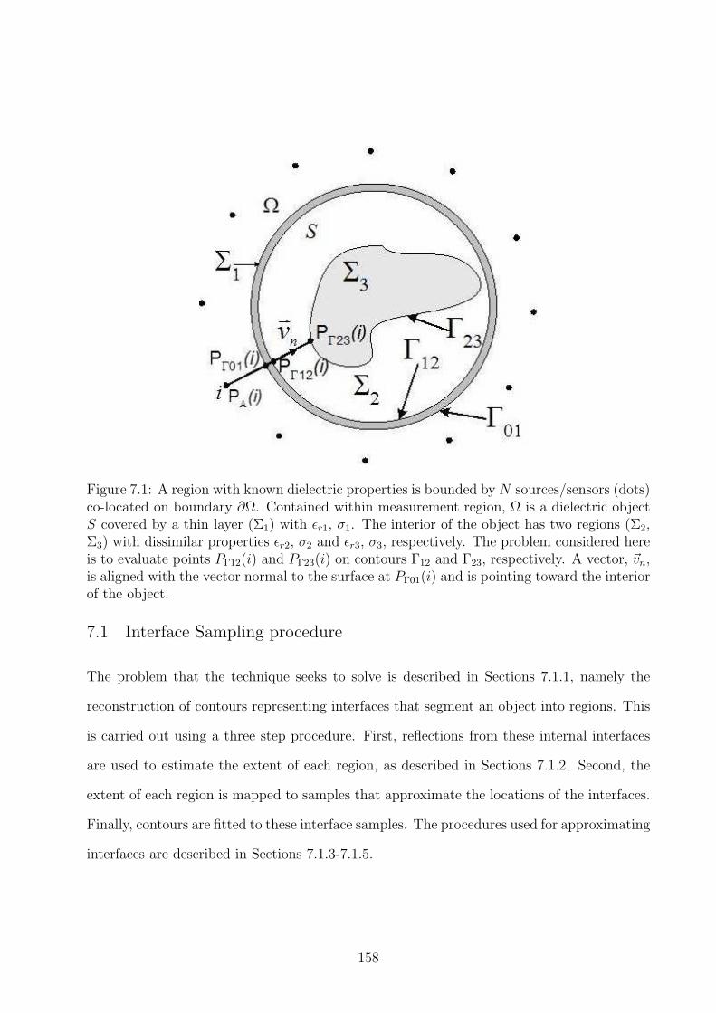
Figure 7.1: A region with known dielectric properties is bounded by N sources/sensors (dots)co-located on boundary ∂Ω. Contained within measurement region, Ω is a dielectric objectS covered by a thin layer (Σ1) with ǫr1, σ1. The interior of the object has two regions (Σ2,Σ3) with dissimilar properties ǫr2, σ2 and ǫr3, σ3, respectively. The problem considered hereis to evaluate points PΓ12(i) and PΓ23(i) on contours Γ12 and Γ23, respectively. A vector, ~vn,is aligned with the vector normal to the surface at PΓ01(i) and is pointing toward the interiorof the object.
7.1 Interface Sampling procedure
The problem that the technique seeks to solve is described in Sections 7.1.1, namely the
reconstruction of contours representing interfaces that segment an object into regions. This
is carried out using a three step procedure. First, reflections from these internal interfaces
are used to estimate the extent of each region, as described in Sections 7.1.2. Second, the
extent of each region is mapped to samples that approximate the locations of the interfaces.
Finally, contours are fitted to these interface samples. The procedures used for approximating
interfaces are described in Sections 7.1.3-7.1.5.
158

7.1.1 Problem Description
Fig. 7.1 illustrates the problem of interest. An object S is covered by a thin outer layer and
the interior has two regions with dissimilar dielectric properties. We assume that the regions
are segregated from each other by distinct interfaces. The goal is to locate the interfaces in
order to identify the major regions that dominate the internal structure of S.
To achieve this goal, the object is placed in a measurement region, Ω, and a source
element i located at PA(i) illuminates S with an UWB electromagnetic pulse. A sensor,
located at the same location as the source, records the resulting backscattered fields. A
full set of reflection data consists of moving the source/sensor pair to N locations on the
periphery, ∂Ω, of the measurement region.
The problem considered is, given that S is illuminated by source element i at PA(i),
extract information from the resulting backscattered fields to evaluate points PΓ12(i) and
PΓ23(i) on contours Γ12 and Γ23, respectively. Moreover, repeating the process for N source
locations, find the corresponding contours that approximate the interfaces from the respective
sets of N points. Unlike the technique proposed in the previous Chapters, the points on the
interfaces are not determined using a ray that connects PA(i) to a point, P0, at the centre
of a region of interest (refer to Section 5.1). Instead, a vector, ~vn, is aligned with the vector
normal to the surface at PΓ01(i) and is pointing toward the interior of the object as shown
in Fig. 7.1. The technique uses this vector to map points to the interfaces and is described
in Sections 7.1.3-7.1.5.
7.1.2 Estimating the extent of a region
The reflections from interfaces are estimated using the procedure presented in Chapters 4
and 5, whereby a sensor receives reflection data to identify locations on interfaces. This is
accomplished with the RDD algorithm that estimates the time-of-arrival of reflections from
interfaces and is described in Section 5.1.1. Just as in Section 5.1.1, we do not assume exact
159

Figure 7.2: Flow-chart of the three-step procedure used to estimate the scaling factor αand TOA parameter τ for each reflection contained in the backscattered data y(t). Each ofscaled and time-delayed version of the reference signal models a reflection from an interfaceseparating the object’s different dielectric regions. At each step, prior information aboutan interface (e.g., geometrical and/or dielectric properties) may be incorporated into thereference signal ri(t).
knowledge of the transmitting signal, but use a reference signal selected to adapt to the
physical behavior exhibited for near-field applications. The procedure used to acquire the
reference signals is described in Section 7.2.3.
Each scaled and time-delayed version of the reference signal represent a reflection from
an interface separating the object’s different dielectric regions, so the TOA parameter may
be calculated with this information. The reference signal used in (5.1) may incorporate prior
information about an interface to improve the model of the reflection from this interface.
Since prior information may be available for each interface, the algorithm is adapted to use
multiple reference signals (i.e., one reference signal for each interface) to estimate reflections
160
contained in the recorded data using the three step procedure shown in Fig. 7.2. The
procedure was first presented and evaluated using data generated with 2D numerical models
illuminated with point sources in Chapter 5. For this study, the feasibility of this approach
is evaluated in a more practical scenario using experimental models illuminated with UWB
sources/sensors.
Once the reflection from each of the three interfaces has been identified, the TOAs are
used to estimate the thickness or extent of each region near the source antenna. For sensor i,
the extent of region j is estimated using the difference in TOA between successive reflections:
∆τj(i) = τj+1(i) − τj(i). (7.1)
The extent of layer j near antenna i, wj(i), is estimated as:
wj(i) =∆τj(i)c0103
2√ǫrj
, (mm) (7.2)
where c0 = 2.9979 108 m/s is the speed of light in free space and ǫrj is the estimated average
relative permittivity of the jth region of interest. We assume that the average dielectric
properties of each region are approximately known. For example, this information may
be incorporated into a microwave tomography system which is used to iteratively refine
estimates of the regional dielectric properties. An example of this integration is provided in
Chapter 6. The extent of each region is used to form points that approximate the locations
of Γ01, Γ12, and Γ23. This is described next.
7.1.3 Estimating the skin surface
The surface Γ01 of the outer thin skin layer shown in Fig. 7.1 may be sampled via a laser
[142] or using microwaves. A surface estimation procedure using microwaves is outlined in
Section 7.2.2. This contour is estimated from the L samples PΓ01(l)Ll=1 (where L ≥ N)
using least squares fitting to the data of cubic spline functions [146] [147].
161
7.1.4 Estimating the skin/region2 interface
Points that approximate the location of Γ12 are mapped from the set of surface samples
PΓ01(l)Ll=1 using the estimated extent of the thin layer. The procedure presented in Chapter
5 maps surface points to Γ12 along a ray that connects each point to the center of the object.
This Chapter uses the following alternative approach whereby each surface point is mapped
to the interior using a ray aligned with the surface normal. First, given a surface sample
PΓ01(l), a local approximation of the object’s profile at PΓ01(l) is computed from a subset of
neighbouring surface samples using least squares fitting to the data of cubic spline functions
[146] [147].
Next, a plane tangential to this local approximation of the profile at PΓ01(l) is estimated.
A vector, ~vn, aligned with the normal to this plane but pointing toward the interior of the
object is then computed. The mean skin thickness, w1,avg, is estimated from (7.2) over the
N sensors. The point PΓ01(l) is then translated along a line in the direction of ~vn a distance
of w1,avg to form a new point PΓ12(l) as shown in Fig. 7.1. The process is repeated for all L
surface points. Contour Γ12 is formed from PΓ12(l)Ll=1 using [146] [147] which is the same
least squares fitting to the data of cubic spline functions method used to fit the outer surface
Γ01. This contour modeling is different than the method used in Chapter 5 which uses a
monotone piecewise cubic interpolation technique. The difference between the estimated,
w1,avg, and actual, w1,avg, average skin thickness is used as a measure of the accuracy of the
algorithm to estimate the extent of thin layers and is given by
Error(w1(i)) = w1,avg − w1,avg. (mm) (7.3)
7.1.5 Estimating the region 2/region 3 interface
For the ith sensor located at PA(i) with known coordinates and a known distance w0 from
Γ01, the problem considered here is to evaluate PΓ23(i) on interface Γ23. The basic idea used
to achieve this is to use the extents of the regions calculated in the first step of the procedure
162

Table 7.1: Dielectric properties of cylindrical model elements.
ǫinf ǫS σ τ Description
2.41 2.52 0.0088 27.84 Canola oil [148]4.00 37.0 1.10 7.20 Damp skin [38]6.01 77.43 1.62 9.41 Inclusions 1-3[149]8.79 74.86 3.10 9.50 Inclusion 4[149]7.80 72.57 4.37 9.07 Inclusion 5[149]
described in Section 7.1.2 to compute the distance d(i) from PA(i) to PΓ23(i) given by:
d(i) ≈ w0 + w1,avg + w2(i), (mm) (7.4)
where w1,avg is the estimated mean skin thickness, and w2(i) is the Γ12-to-Γ23 distance and
is calculated using (7.2). The mapping assumes that the antenna axis is aligned along ~vn(i)
which is calculated as described in Section 7.1.4. This means that the antenna is aligned with
the surface normal and pointing toward the interior of the object. Point PA(i) is translated
distance d(i) in direction ~vn(i) to form point PΓ23(i). The process is repeated for all N
antenna positions resulting in PΓ23(i)Ni=1. This procedure is different from the method
presented in Chapter 5 where the point is translated along a ray that connects the sensor to
the centre of the object. Contour Γ23 is formed from using [146] [147] which is the same least
squares fitting to the data of cubic spline functions method used to fit the outer surface Γ01.
To measure the effectiveness of this procedure to estimate points on Γ23, the mean Eu-
clidean distance between the estimated point PΓ23(i) and corresponding actual point PΓ23(i)
on contour on Γ23 is computed with
ME(PΓ23) =1
N
N∑
i=1
‖PΓ23(i) − PΓ23(i)‖. (7.5)
163

Figure 7.3: Models used for numerical and experimental studies. Properties of skin (brown),region 2 (green), and inclusions (red) shown in Table 7.1. Cases 1, 2, and 3 shown in (a),(b), and (c), respectively
7.2 Description of Models
The techniques described in Section 7.1 are tested with numerical models reported in Sec-
tion 7.2.1 for which properties and geometries are known exactly. Experimental data are
collected with similar models, as described in Section 7.2.2. For both types of models, ref-
erence functions incorporating various levels of information about the object are tested, as
described in Section 7.2.3.
7.2.1 Numerical models
The algorithm’s feasibility to identify the internal structure of objects is first evaluated using
cylindrical models illuminated with a realistic source/sensor. The simulations are carried out
with the finite-difference time-domain (FDTD) method using SEMCAD X (SPEAG, AG,
Zurich, Switzerland). Three cases are investigated and are shown in Fig. 7.3. All cases are
based on a cylindrical model in which a 1.8 mm thick skin layer with dispersive dielectric
properties is placed on a 96 mm ∅ cylinder. Canola oil fills the interior of the cylinder. The
164

dielectric properties of each element are listed in Table 7.1. For Case 1 (Fig. 7.3(a)), a single
cylindrical 50.9 mm ∅ inclusion with an interior consisting of 1% saline is inserted into the
model (inclusion 1).
The second cylindrical model (case 2 shown in Fig. 7.3(b)) is the same as the first except
that inclusion is replaced with two smaller cylinders having the following properties: (1) a
28.5 mm ∅ cylinder filled with 2% saline (inclusion 2), and (2) a 22.3 mm ∅ cylinder filled
with 3% saline (inclusion 3).
The third cylindrical model (case 3 shown in Fig. 7.3(c)) is the same as the second except
that two additional cylinders are included having the following properties: (1) a 9.4 mm ∅
cylinder filled with 1% saline (inclusion 4), (2) a 16.0 mm ∅ cylinder inclusion filled with
1% saline (inclusion 5).
A balanced antipodal Vivaldi antenna with director (BAVA-D) [66] is placed 1.5 mm from
the surface of the model. Both the model and the antenna are immersed in Canola oil. The
model is illuminated with a Gaussian differentiated pulse [150] having a -3 dB bandwidth
of 3.5 GHz and fmax = 3.795 GHz. Here, fmax is the frequency where the magnitude of the
spectrum of the pulse is 10% of its maximum magnitude. The resulting backscattered fields
are recorded with the same antenna. This process is repeated with the antenna positioned
in a single plane and scanned to 40 equally spaced positions around the model. Calibration
is performed to remove the contributions from the antenna and the external environment.
Finally, the data are normalized to the maximum positive value of reflected signals. It is
assumed that Γ01 is sampled with a laser as described in [142] (i.e., it is assumed that the
location of the surface is known with high accuracy).
7.2.2 Experimental models
The experimental system is shown in Fig. 7.4 and is described in [18]. It consists of a tank
of Canola oil and uses two BAVA-D antennas positioned directly opposite each other. Each
sensor collects reflection data. To collect measurements, the antennas are placed 148 mm
165

Figure 7.4: Experimental system used to acquire S11 and S22 data. The model used for case1 is shown.
below the top of the tank and mounted on a sliding arm as shown in Fig. 7.4. We note
that minimal coupling between the two antennas is expected, and collecting signals with 2
antennas permits us to examine the repeatability of the results.
The shape and size of the cylindrical models used for this part of the investigation are
similar to the numerical models used in Section 7.2.1 and shown in Fig. 7.3. Each cylindrical
inclusion consists of a Plexiglas tube filled with a saline solution. The exact location of each
inclusion is not exactly known. The electrical properties are expected to be similar to those
assumed for the simulations. Material with ǫr=34.3, σ=4.25 S/m (averaged over 1.0 to 10
GHz) and having a mean thickness of 1.8 mm is used to mimic the skin layer. This layer
is constructed from a polyurethane plastic sheet (LD-32, Emerson and Cuming Microwave
Products) having dispersive properties. Holders at the top and bottom of the model are
used to form this thin flexible layer into a 96 mm ∅ cylinder.
Each antenna is adjusted 1.5 mm from the surface of the model using a knurled wheel.
A digital caliper is attached to the mechanism to measure accurate separation distances.
Coaxial cables connect each antenna to a vector network analyzer (PNA-X, Agilent Tech-
nologies, Palo Alto, CA, USA) via a coaxial cable. To increase sensitivity, measurements are
166

performed with an intermediate frequency (IF) bandwidth of 1 KHz and a port power level
of 10 dBm. These settings produce an 80 dB dynamic range at the antenna port without the
need for additional averaging. A total of 1601 discrete frequencies (or sweeps) are recorded
over a range of 0.5-12 GHz. The model is rotated (i.e., the position of the antennas and
cables are fixed) to 40 equally spaced angular positions (over 360 degrees) and reflection
coefficients for each antenna (i.e., S11 and S22) are recorded at each position.
Typically, measurement systems would acquire surface samples with a laser. However, for
this study, we approximate the outer surface with microwaves using the following procedure.
First, a reference distance, w0,ref , is accurately measured with a digital caliper at one of the
antenna positions (i.e., the reference position). The reflection data decomposition algorithm
is used to identify the reflection off of the outer surface and the TOA of this reflection is
estimated. The reflection from the surface at different locations for the remaining antenna
positions is identified and the corresponding TOA is determined. The difference in the TOA
between each reflection and the reference TOA is then evaluated and the distance, w0(i), is
determined using (7.2). The distance from the antenna to the surface is estimated using
w0(i) = w0,ref + ∆w0(i). (mm) (7.6)
For example, suppose the reference antenna is 1.5 mm from the surface and the TOA of the
surface reflection is approximately 1442.8 ps. At another position, the TOA of the surface
reflection is 1433.1 ps, so it arrives 9.7 ps before the surface reflection at the reference
position. Substituting this value into (7.2) and with ǫr = 2.41, it is determined that the
antenna is 0.94 mm closer to the surface at this location compared to the reference position
(i.e., it is 0.56 mm from the surface). Using this distance and the antenna coordinates leads
to an approximation of the location of the surface sample, PΓ01(i). Repeating this procedure
for all N antenna positions results in the set of surface samples PΓ01(i)N
i=1. The techniques
described in Sections 7.1.3 and 7.1.4 approximate the interfaces Γ01 and Γ12.
167
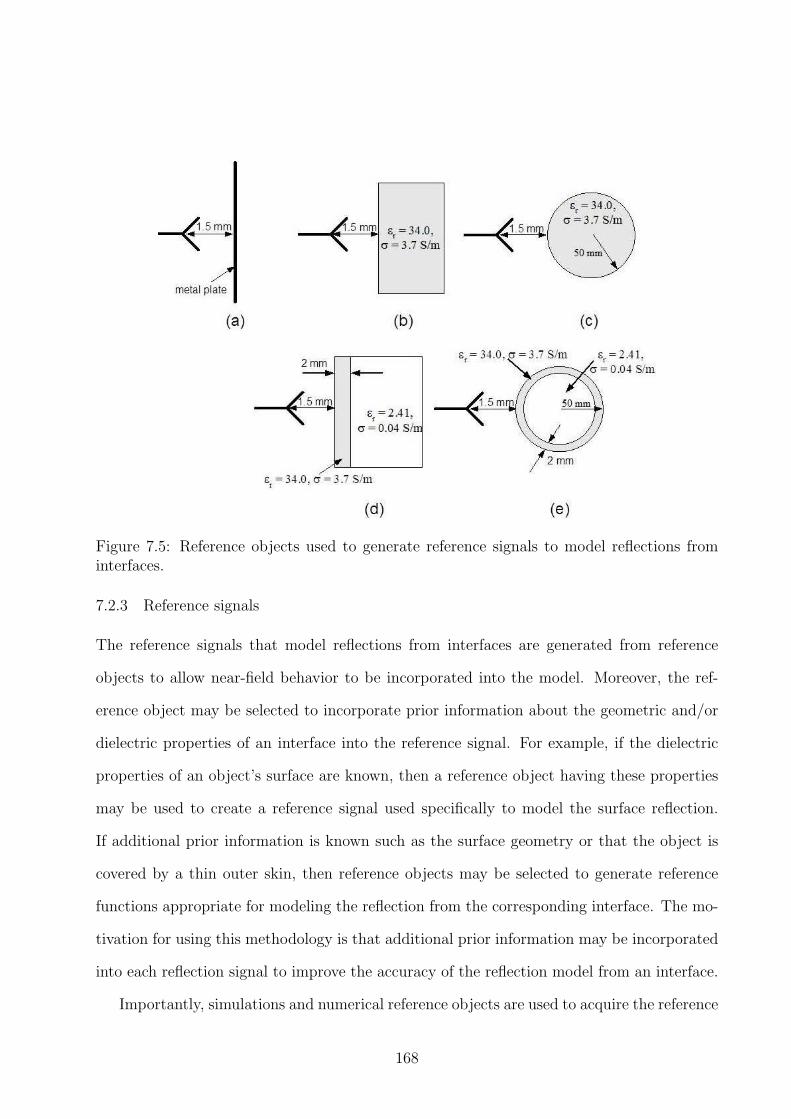
Figure 7.5: Reference objects used to generate reference signals to model reflections frominterfaces.
7.2.3 Reference signals
The reference signals that model reflections from interfaces are generated from reference
objects to allow near-field behavior to be incorporated into the model. Moreover, the ref-
erence object may be selected to incorporate prior information about the geometric and/or
dielectric properties of an interface into the reference signal. For example, if the dielectric
properties of an object’s surface are known, then a reference object having these properties
may be used to create a reference signal used specifically to model the surface reflection.
If additional prior information is known such as the surface geometry or that the object is
covered by a thin outer skin, then reference objects may be selected to generate reference
functions appropriate for modeling the reflection from the corresponding interface. The mo-
tivation for using this methodology is that additional prior information may be incorporated
into each reflection signal to improve the accuracy of the reflection model from an interface.
Importantly, simulations and numerical reference objects are used to acquire the reference
168

signals. This approach is taken to improve the flexibility in the choice of reference objects
that may be used to acquire the prior information and to simplify the procedure implemented
to generate the reference signals. Otherwise, acquiring this information using experimental
methods is formidable. To evaluate the effectiveness of this strategy in a practical scenario,
reference functions are generated using the following procedure. First, for the most general
application where no prior information is available, the reflection from a metal plate is used
as a reference function. A numerical plate is placed 1.5 mm from the UWB antenna as
shown in Fig. 7.5(a). Both the plate and antenna are immersed in canola oil. A simulation
is carried out whereby the plate is illuminated with a Gaussian differentiated pulse having a
-3 dB bandwidth of 3.5 GHz. The resulting backscattered fields, y1(t), are recorded with the
same antenna. The simulation is repeated without the metal plate to acquire the antenna
only signal. Finally, the reference signal, r1(t), is recovered by subtracting the signal recorded
with only the antenna present from y1(t).
A dielectric half-space (i.e., slab with infinite width and extent) as shown in Fig. 7.5(b)
is used for the reference object if prior information about the dielectric properties of the
object’s surface is known. The procedure used with the metal plate is repeated for the
slab to extract the surface reference signal. If prior information about both the general
geometrical and dielectric properties of the surface of the object is known, then the cylinder
shown in Fig. 7.5(c) is used for the reference object. The same procedure is used to extract
the reference signal from the surface of the cylinder.
There may be applications where it is known that the object is covered by a thin outer
layer and the general dielectric properties of this layer and the interior of the object are
known. For this scenario, the layered dielectric slab as shown in Fig. 7.5(d) is used for the
reference object. A simulation is carried out with the planar model and the backscattered
fields, y2(t), are recorded. The signal recorded with only the antenna present is subtracted
from this signal to recover y12(t), which is the combined reflections from the surface, r1(t)
169

and the skin/interior interface, r2(t) (i.e., y12(t) = r1(t) + r2(t)). The simulation is repeated
with the homogeneous slab shown in Fig. 7.5(b). The signal with only the antenna present
is subtracted from the resulting signal to recover the surface reflection, r1(t). This reflection
is used to recover the reflection from the skin/interior interface (i.e., r2(t) = y12(t) − r1(t)).
Finally, both the general shape and the general dielectric properties of the object may be
known. For this scenario, the reference object is replaced with the concentric cylinder shown
in Fig. 7.5(e). The same procedure as described for the two layer planar model may be used
to recover reference signals for the surface and the skin/interior interface corresponding to
reference signals r1(t) and r2(t), respectively.
7.3 Numerical results
7.3.1 Case 1
The internal geometric properties are first extracted by assuming no prior information about
the model. Therefore, the reference signal from a metal plate (Fig. 7.5(a)) as described in
Section 7.2.3 is used to model the reflection from all three interfaces. The distance measures
described by (7.3) and (7.5) are applied to the results to evaluate the performance of the
algorithm. As shown in Table 7.2, the mean distance between the actual and estimated
point on the internal interface Γ23 is 0.53 mm and the estimated and actual average skin
thickness differ by 0.13 mm. The result implies that without any prior knowledge about the
object, the algorithm is able to accurately estimate the location of the interfaces. Estimates
of the interior regions of the object evaluated using reference signals from a metal plate are
shown in Fig. 7.6(a). These results illustrate the accuracy with which the interior region is
estimated.
Next, we assume prior knowledge of the approximate dielectric properties of the sur-
face by using a reflection from a dielectric slab (Fig. 7.5(b)) as described in Section 7.2.3.
The same reference signal is used to model the reflection from all three interfaces. The
170

Table 7.2: Numerical data: Accuracy of interface points.
Case 1 Case 2 Case 3 Case 1-3Reference ME(PΓ23) ME(PΓ23) ME(PΓ23) Error(w1,avg)Object (mm) (mm) (mm) (mm)
metal plate 0.53 15.6 21.54 0.131 layer slab 0.55 4.72 3.64 0.041 layer cyl. 0.35 5.07 3.45 0.162 layer slab 0.39 4.70 3.52 0.052 layer cyl. 0.55 4.95 3.75 0.15
Figure 7.6: Numerical results showing interface samples (yellow squares), actual (red), andapproximated (blue) region 3. Approximations of skin and region 2 shown in brown andgreen, respectively. Cases 1, 2 and 3 shown in (a), (b), and (c), respectively.
171

result shown in Table 7.2 implies that this prior knowledge does not improve the accuracy
of the estimated interface location. We continue with this methodology, each time incorpo-
rating additional prior information about the skin surface, the skin surface properties, the
skin/interior interface, and the dielectric properties of the interior of the object into the
reference signals. The results shown in Table 7.2 imply that this prior information does not
significantly improve the accuracy of the estimation. We note that the mean skin thickness
estimation does not depend on the interior of the numerical model studied. The Table 7.2
results imply that the skin is estimated accurately regardless of the reference signal used.
7.3.2 Case 2
From Fig. 7.3(b) we observe that the complexity of Region 3 has increased compared to
Case 1 in that it consists of two isolated scatterers. As with Case 1, the internal geometrical
properties are first extracted by assuming no prior information about the object. Hence, a
reference signal from a metal plate is used to model the reflection from all three interfaces.
The mean distance between the actual and estimated point on the internal interface Γ23
is 15.6 mm. The result implies that without any prior knowledge about the object, the
algorithm is unable to accurately estimate the location of this more complicated interface.
Next, we assume that prior knowledge of the approximate dielectric properties of the
surface by using the reflection from a dielectric slab (Fig. 7.5(b)) for the reference signal.
The same reference signal is used to model the reflection from all three interfaces. The result
shown in Table 7.2 (ME(PΓ23)) = 4.72 mm) implies that this prior knowledge significantly
improves the accuracy of the estimation of the interface location compared to the result
obtained using the reflection from a metal plate.
We now assume prior information about both the general shape and dielectric properties
of the object’s surface by using a cylindrical reference object as shown in Fig. 7.5(b) to
generate the reference signal to model the reflection from all three interfaces. The result
(ME(PΓ23) = 5.07 mm) implies that this additional prior information about the shape of
172

the surface does not improve the estimate of the interface location.
Prior knowledge of the skin thickness, the dielectric properties of the surface, and the
dielectric properties of region 2 is incorporated into the surface reflection (r1(t)) and the
skin/interior reflection (r2(t)) using the 2 layer slab as shown in Fig. 7.5(d) for the reference
object. The surface reflection is also used to model the reflection from the region 2/region 3
interface. The result in Table 7.2 (ME(PΓ23) = 4.70 mm) implies that this additional prior
information about skin layer provides only a marginal improvement in the ability of the
algorithm to extract features related to Γ23. Finally, in addition to the prior knowledge of
the skin thickness and dielectric properties of the skin and interior, prior information about
the shape of the surface and the skin region is incorporated into the models of the first and
second reflections. The result in Table 7.2 implies that this additional shape information
does not improve the estimate of the interface location.
Estimates of the interior regions of the object obtained using reference signals from a 2
layer cylinder reference object are shown in Fig. 7.6(b). As expected, the algorithm is unable
to extract spatial details related to the individual scatters that comprise region 3. Instead
more general information about the region is extracted. This is discussed in greater detail
in Section 7.5.
7.3.3 Case 3
For this case, region 3 consists of a multiple isolated objects that are clustered together in the
center of the model. Compared to the previous two cases, the contour describing Γ23 is more
complex. Extracting the internal geometrical properties of the object using the reflection
from a metal plate is ineffective in this scenario as the mean distance between the actual
and estimated point on the internal interface Γ23 is 21.54 mm. As with the previous cases,
we continue with this methodology, each time assuming additional prior information about
the skin surface, the skin surface properties, the skin/interior interface, and the dielectric
properties of the interior of the object into the reference signals. The results shown in
173

Table 7.2 imply that prior information about the surface, the skin layer, and the dielectric
properties about the interior of the object improves the accuracy of the estimation. However,
prior shape information does not have a significant impact on the accuracy of the estimation.
Estimates of the interior regions of the object obtained using reference signals from the 2
layer slab reference object are shown in Fig. 7.6(c). Similar to Case 2, the closed contour used
to model the region 2/region 3 interface is unable to extract spatial details related to multiple
disconnected homogeneous scatterers. Instead only general information is extracted. This is
discussed in greater detail in Section 7.5.
7.4 Experimental results
The experimental data are processed using the same methodology as is used for data from
the numerical models. That is, we initially assume no prior information about the object
and use the reference signal from a metal plate to model the reflection from each interface.
Instead of using a numerical metal plate, the reference signal is acquired experimentally
with an actual metal plate. Next, we determine if prior knowledge about the target object
improves the accuracy of the results. In particular, we assume prior knowledge of the approx-
imate dielectric properties of the object’s surface by using the reflection from a numerical
dielectric object as described in Section 7.2.3. The same reference signal is used to model
the reflection from all three interfaces. We continue with this methodology, each time incor-
porating additional prior information about the skin surface, the skin surface properties, the
skin/interior interface, and the dielectric properties of the interior of the object into the ref-
erence signals. The distance measures described by (7.3) and (7.5) are applied to the results
to evaluate effectiveness of the algorithm to extract an object’s internal features in an exper-
imental setting. We note that the exact inclusion locations within the interior are unknown,
but are estimated using the design drawings used to fabricate the models. This uncertainty
contributes to the size of the distance measure ME(PΓ23). Furthermore, estimation errors
174

Table 7.3: Numerical data: Accuracy of interface points.
Case 1 Case 2 Case 3 Case 1-3Reference ME(PΓ23) ME(PΓ23) ME(PΓ23) Error(w1,avg)Object (mm) (mm) (mm) (mm)
metal plate 1.74 9.51 5.52 0.151 layer slab 1.67 4.80 4.13 0.311 layer cyl. 1.70 4.95 4.16 0.382 layer slab 1.83 4.79 3.55 0.272 layer cyl. 1.82 5.00 3.08 0.40
Figure 7.7: Experimental results showing interface samples (yellow squares), actual (red),and approximated (blue) region 3. Approximations of skin and region 2 shown in brown andgreen, respectively. Cases 1, 2 and 3 shown in (a), (b), and (c), respectively.
of w0(i) are introduced when evaluating the surface location using the procedure outlined
in Section 7.2.2. Since these values are used to approximate an interface point PΓ01(i), the
estimation errors also increase the size of ME(PΓ23).
The results are presented in Table 7.3. We note that, although two antennas are used
for measuring the backscattered data, results are presented for the reflection data from only
one of the sensors. As expected, the results are approximately equivalent for both antennas.
Finally, we note that the skin thickness estimation that is provided in Table 7.3 is the same
for all three cases (i.e., it is model independent).
175

7.4.1 Case 1
Similar to the numerical model results, prior information does not improve the accuracy of the
interface location estimates. For this example, the error in the estimated interface locations
has increased significantly. Possible factors contributing to the error include errors in the
surface estimation and uncertainty about the exact location of the inclusion as discussed
in the introduction to Section 7.4. Estimates of the interface location along with regions
identified using the reference signals from a concentric cylinder are shown in Fig. 7.7(a). For
this example, we observe that the major regions that dominate the internal structure of the
object are identified.
7.4.2 Case 2
Unlike the previous case, the experimental (Table 7.3) and numerical (Table 7.2) results are
comparable. Prior knowledge about the general dielectric properties of the object’s surface
improves the accuracy of the interface sample. Critically, this prior information is derived
from numerical objects as described in Section 7.2.3. This is significant since the results
suggest that the prior information about the object’s surface is effectively incorporated into
a reference signal acquired from the reflection off of a numerical object. Similar to the
numerical case, the results suggest that prior information about the object’s shape or skin
thickness does not significantly improve the accuracy of the results. The internal features
extracted using reference signals from a concentric cylinder as a reference object are shown
in Fig. 7.7(b). Possible source of errors are described in the previous case, i.e., there is
uncertainty in the exact location of the cylinders and the location of the surface. Similar
to the numerical case, the technique is unable to extract spatial details related to multiple
disconnected homogeneous scatterers. Instead general information is extracted.
176

7.4.3 Case 3
Similar to the previous case, the results presented in Tables 7.2 and 7.3 suggest that the
numerical and experimental results are very comparable. Unlike the numerical scenario, we
observe that for the experimental scenario, prior information about the skin thickness (i.e.,
using a 2 layer slab or a concentric cylinder as a reference object) improves the accuracy of
the interface location estimate. The internal features extracted using reference signals from
a concentric cylinder as a reference object is shown in Fig. 7.7(c). Similar to Case 2, the
algorithm is unable to extract detailed spatial features of the interface. However, it is able
to extract the general underlying structure.
7.5 Discussion
For both the numerical and experimental studies presented in Sections 7.3 and 7.4, respec-
tively, it is observed that the algorithm is unable to extract detailed features related to
concave regions of the interface from the reflection data. We note that the reflection data
recorded by the receiver may be considered as a sum of contributions from reflections prop-
agating along different paths; each reflection has a different propagation time and scaling
factor. The procedure outlined in Section 7.1.2 is used for determining the dominant scat-
terer associated with the third reflection. Furthermore, the procedure assumes that this
dominant scatterer is located along a straight path from the antenna to the interface aligned
with the vector normal to the breast surface. Hence, the difference in arrival time between
the reflection associated with interface Γ12 and the reflection assumed to be associated with
Γ23 is mapped along this path from the ith antenna to an estimated point on the interface
at distance of d(i) given by (7.4).
For concave regions, such as region 3 of Case 1, this assumption holds and the interface
points may be estimated with reasonable accuracy. However, for Cases 2 and 3, non-concave
spatial variations of the contour are observed. For these scenarios, it is not possible to extract
177

the reflections associated with Γ23 along a straight path. Instead, the dominant scatterer
may be associated with a curved path or with a path that is not aligned with the surface
normal. This leads to propagation times that are shorter than the assumed straight path.
The discrepancy from the assumed straight path model leads to errors in the estimated
location of the interface point. We observe this for a number of interface points shown in
Fig. 7.6(b) and 7.6(c).
Detailed features and the ability to extract isolated scatterers is not possible using this
technique. However, the aim is to extract general features related to the underlying internal
structure of the object. This aim has been achieved, as demonstrated by the results presented
in Figs. 7.6 and 7.7, as well as Tables 7.2 and 7.3. The structural information may serve
as prior information to improve the speed, stability, and accuracy of existing microwave
tomographic methods.
7.6 Conclusion
The effectiveness of a radar-based technique to extract internal structural information from
experimental objects is demonstrated. Importantly, the experimental results obtained are
comparable with the numerical results. This provides a degree of validation of the numerical
evaluation procedures used for the design and verification of effective measurement systems.
For some objects having complicated interiors (e.g., Case 3 has an interior consisting of a
cluster of high contrast scatterers), the results suggest that prior information about the ob-
ject is required to accurately estimate the location of internal interfaces. Importantly, this
prior information may be derived from reflections generated with simulations of numerical
reference objects such as dielectric slabs and cylinders. This provides a convenient and flexi-
ble methodology to acquire prior information about an object. We note that this information
would be very challenging to acquire experimentally.
The results also imply that the algorithm is capable of resolving features related to thin
178

layers in a realistic scenario. For example, many anatomical structures may be characterized
as having one or more distinct thin outer layers (e.g., skin layer, fat layer, muscle layer, etc.).
The technique offers an approach suited for medical applications requiring the identification
of thin layers and layers that are in close proximity to each other. For example, resolving
thin skin and adipose layers in the forearm when reconstructing the dielectric properties as
described in [151] is challenging at the interrogating frequencies utilized by the microwave
tomography system. This technique has the potential to be able to resolve these layers.
Reconstruction methods may benefit by having these layers identified prior to the application
of the microwave tomographic technique.
Thus far, only 2D information (internal structural and regional dielectric property infor-
mation) has been extracted for the object under investigation. In Chapter 8, 3D extensions
of the 2D techniques are presented and applied to 3D scenarios. Specifically, the regional
feature extraction technique is applied to data generated from numerical anthropomorphic
breast models. This includes incorporating the results with microwave tomography.
179

Chapter 8
Extensions of regional estimation of the dielectric
properties of objects to 3D
6 The techniques for identifying the structure of an object and estimating mean dielectric
properties over regions presented in the previous Chapters were developed with 2D models.
In this Chapter, the next step towards the development of this promising approach into a
clinical tool that may be used for a range of medical applications is described. Specifically, the
method is extended so that it may be applied to 3D scenarios in which the target is scanned
with a realistic sensor/source. The methodology used to extend the technique to these
more realistic scenarios is discussed in Section 8.1. The formation of reconstruction models
when the method is applied to numerical data generated with a 3D realistic breast model
is described in Section 8.2. A pseudo-3D reconstruction of the mean dielectric parameter
profiles of a numerical breast model is described in Section 8.3. Finally, conclusions are
provided in Section 8.4.
8.1 Interface sampling procedure
The problem that the technique seeks to solve is described in Section 8.1.1, namely the
reconstruction of surfaces representing interfaces that segment an object into regions. This
is carried out using a three step procedure. First, reflections from these internal interfaces are
used to estimate the extent of each region, as described in Section 8.1.2. Second, the extent
of each region is incorporated into a transformation used to map known points (antenna
locations or points on the exterior surface) to samples that approximate the locations of the
6The parameter estimation results were presented at the Proceedings of the IEEE International Sympo-
sium on Antennas and Propagation and USNC-URSI National Radio Science Meeting, July 8-14, 2012, inChicago, IL, USA.
180

interfaces. Finally, internal interfaces are fitted to these clouds of interface samples. The
procedure used for approximating surfaces is described in Sections 8.1.4-8.1.6. Once the
interface surfaces are estimated, a reconstruction model is formed from these surfaces. The
reconstruction model, which has effectively segmented the interior of the target into regions,
is then incorporated into the MWT method which estimates the mean dielectric properties
over each region. The regional reconstruction technique is described in Section 8.1.7.
8.1.1 Problem Description
We present ideas concerning the recovery of internal structural information in an inverse
problem context. The goal of the proposed approach is to estimate an object’s internal 3D
geometric structure. Specifically, we seek to identify and segment the major regions that
dominate an object’s internal structure. Once the interior of the object is segmented into
regions, a MWT technique estimates the mean dielectric properties over the regions. We
assume that the regions are segregated from each other by distinct boundaries or interfaces.
Defining locations of the interfaces involves analyzing reflections from the object as described
in Chapters 4,5 and 7.
Fig. 8.1 illustrates the problem of interest. An object S is placed in a measurement region
Ω and a source element i located at PA(i) illuminates S with an UWB electromagnetic pulse.
A sensor, located at the same location as the source, records the resulting backscattered fields.
A full set of received data consists of moving the source and sensor pair to N locations in
3D-space on the periphery ∂Ω of the measurement region. The 3D measurement space is
defined by a coordinate system shown in Fig. 8.1.
The object is covered by a thin outer layer and the interior has two regions with dissimilar
dielectric properties. The interior regions are not restricted to be homogeneous, but rather
represent regions that are dominated by a particular material. The interfaces between re-
gions are denoted as Γ01, Γ12 and Γ23, respectively. The problem considered is, given that S
is illuminated by source element i at PA(i), extract information from the resulting backscat-
181

Figure 8.1: A measurement region Ω with known dielectric properties is bound by Nsources/sensors co-located on ∂Ω. Contained within Ω is a dielectric object S covered by athin layer with an outer surface Γ01. The interior of S is separated from the outside layerby Γ12 and has two regions with dissimilar properties segregated by Γ23. The problem con-sidered is to evaluate points PΓ12
(i) and PΓ23(i) on interfaces Γ12 and Γ23, respectively and
to fit surfaces to these data.
tered fields to evaluate points PΓ12(i) and PΓ23
(i) on interfaces Γ12 and Γ23, respectively.
Moreover, repeating the process for N source locations, find the corresponding surface that
approximates the interface from the respective cloud of N points.
8.1.2 Estimating the extent of a region
The first step in the interface sampling procedure is to estimate the extent of each region.
This step is based on the key fact that reflections arise from dielectric contrasts at inter-
faces. Therefore, this procedure extracts information from the backscattered data to estimate
points on these interfaces. The reflections from interfaces are estimated using the following
182

0.5 0.7 0.9 1.1 1.3 1.5 1.7−0.2
−0.1
0
0.1
0.2
0.3
0.4
Time (ns)
Am
plitu
de
(a) Time-domain representation.
0 2 4 6 8 10 12 14 150
0.1
0.2
0.3
0.4
0.5
0.6
0.7
0.8
0.9
1
frequency (GHz)
Nor
mal
ized
Mag
nitu
de
(b) Frequency-domain representation.
Figure 8.2: A waveform propagates 35 mm into breast tissue. The initial waveform and itsspectrum are shown in red. The resulting waveform and spectrum after it propagates 35 mminto fatty breast tissue are shown in blue.
procedure. As presented in Chapters 4 and 5 and repeated here for clarity, a sensor receives
reflection data to identify locations on interfaces. This is accomplished with the RDD al-
gorithm that estimates the time-of-arrival of reflections from interfaces and is described in
Section 5.1.1. The TOAs are used to estimate the thickness or extent of each region near the
source antenna with the assumption that the average dielectric properties of each region are
known. For sensor i, the extent of region j is estimated using the difference in TOA between
successive reflections:
∆τj(i) = τj+1(i) − τj(i) (s). (8.1)
183

The extent of layer j near antenna i, ωj(i) , is estimated with
wj(i) =vg,j∆τj(i)103
2(mm) (8.2)
where vg,j is the group velocity of the waveform in region j. Group velocity is used for this
calculation since the object is illuminated with an UWB pulse comprised of many spectral
components propagating in media that are typically dispersive. The methodology used to
calculate the group velocity is described next.
8.1.3 Group velocity
The concept of group velocity is based on the assumption that the pulse is formed due to the
constructive summation of many spectral components which, in turn, implies that the phase
of each of these components (i.e., the components that add constructively) is equivalent
(cf [152]). Moreover, phase equivalence infers that the phase of each component that adds
constructively to form the pulse is independent of wavenumber, k, near some value of k.
This vague condition leads to ambiguity about which value of k to use for evaluating the
group velocity. As a remedy, we suggest using a strategy based on the key idea that group
velocity may be estimated at the value of k that dominates the pulse and corresponds to the
Fourier component with the largest magnitude.
The expected spectral content of the pulse is determined a priori by running numeri-
cal simulations of a model of the medium in which the wave is propagating. The Fourier
components of the pulse are computed and the spectral content of the pulse is examined
at various points as it propagates through the medium. For example, a pulse after it has
propagated 35 mm in fatty breast tissue is shown in Fig. 8.2(a). The transmitted pulse is
not just a scaled-down version of the initial pulse, but has a different shape. In Fig. 8.2(b)
it is observed that the higher frequency components of the pulse are attenuated more than
the lower frequency components which effectively leads to a spectral shift of the transmitted
waveform. Moreover, the frequency of the Fourier component with the largest magnitude
184

has decreased by 0.24 GHz after the pulse has transmitted through the tissue. The angular
frequency, ωmax, of the Fourier component with the largest magnitude is used to calculate the
wavenumber that dominates the pulse. The wavenumber is complex, so the phase constant,
β, is the imaginary part of jk and is approximated by assuming a uniform plane model given
by [153]
β(ω) = ω
√√√√µǫ
2
(√1 +
( σωǫ
)2
+ 1
), (8.3)
where ǫ = ǫ0ǫr; ǫ0 = (1/36π)10−9 is the permittivity of free space; ǫr = ℜǫ∗(ω) is the
relative permittivity of the medium; σ = −ωǫ0ℑǫ∗(ω) (S/m) is the conductivity of the
medium; µ = µ0µr is the permeability of the medium; µ0 = 4π10−7 is the permeability of
free space; µr = 1 is the relative permeability of the medium. The complex permittivity,
ǫ∗(ω), of the dispersive medium is evaluated using a single pole Debye model [154] expressed
as (based on the derivation given by [155]),
ǫ∗(ω) = ǫ∞ +ǫs − ǫ∞1 + jωτ
+σs
jωǫ0, (8.4)
where ǫs and ǫ∞ are the dielectric constants at zero (static) and infinite frequency, respec-
tively; ω (rad/s) is the angular frequency; σs (S/m) is the conductivity at zero (static)
frequency; and τ (s) is the relaxation time constant. The Taylor expansions of β(ω + ∆ω)
and β(ω−∆ω) at ωmax are used to obtain a central difference approximation of the gradient
of the phase constant that is fourth order accurate and is given by [156],
∂β(ω)/∂ω ≈ (β−2 − 8β−1 + 8β+1 − β+2)/12∆ω, (8.5)
where β−2 = β(ω−2∆ω), β−1 = β(ω−∆ω), β+1 = β(ω+∆ω), and β+2 = β(ω+2∆ω). The
gradient obtained with (8.5) is used to estimate the group velocity at ωmax using [157],
vg = [∂β(ω)/∂ω]−1∣∣∣ω=ωmax
. (8.6)
Substitution of (8.6) into (8.2) allows the extent of a region to be approximated. We note that
the group velocity calculation and the corresponding evaluation of the extent of a region are
185

incorporated into the iterative parameter estimation algorithm described in Section 8.1.7. In
particular, the phase constant calculated with (8.3) uses dielectric property values estimated
with a parameter estimation algorithm.
The group velocity calculation is compared with two other measures of velocity: the
relative velocity, vr, and the weighted mean phase velocity, vp. The relative velocity is
determined with,
vr = c0/√ǫr, (m/s) (8.7)
where c0 = 2.998×10⁸ m/s is the speed of light in free space. The mean relative permittivity,
ǫr, in (8.7) of the layer is evaluated over a frequency range ω1 to ωNωwith,
ǫr =1
Nω
Nω∑
i=1
ǫr(ωi), (8.8)
where Nω is the total number of spectral components used to determine ǫr; and ǫr(ωi) is
the real part of (8.4) evaluated at ωi using the Debye parameters for the tissue layer. The
weighted mean phase velocity is calculated by weighting the phase velocity of each Fourier
component by the magnitude of the component. Therefore, more weight is placed on those
Fourier components that dominate the spectrum of the pulse when calculating the mean
phase velocity. The weighted mean phase velocity is calculated using,
vp =
∑Npi=1ws,ivp,i(ωi)∑Np
i=1ws,i
, (m/s) (8.9)
where Np is the number of Fourier components of the pulse after it has propagated a distance
through the medium; ws,i is the magnitude of the ith Fourier component normalized to the
maximum magnitude of the spectrum of the pulse (i.e., it assumes a value between 0 to 1);
and vp,i(ωi) is the phase velocity of the ith Fourier component with frequency ωi. The phase
velocity of the ith Fourier component that has a frequency of ωi (rad/s) in (8.9) is computed
with [153],
vp,i(ωi) =ωi
β(ωi), (m/s) (8.10)
where β(ωi) is the phase constant computed with (8.3) at ωi.
186

Table 8.1: Group velocity (vg), relative velocity (vr), and weighted mean phase velocity (vp)of a pulse at various distances as it propagates within fatty tissue. The frequency, fmax, isthe frequency of the maximum Fourier component of the spectrum.
Distance fmax vg vr vp dev(vg, vr) dev(vg, vp)(mm) (GHz) ×108(m/s) ×108(m/s) ×108(m/s) (%) (%)
0 4.858 1.482 1.43 1.422 3.5 4.010 4.774 1.479 1.43 1.418 3.3 4.120 4.711 1.477 1.43 1.414 3.1 4.230 4.685 1.475 1.43 1.411 3.0 4.340 4.572 1.472 1.43 1.408 2.8 4.350 3.878 1.449 1.43 1.405 1.3 3.0
The group velocity, vg, the relative velocity, vr, and the weighted mean phase velocity,
vp, of a pulse at various distances as it propagates through fatty tissue (ǫ∞ = 3.14; ǫs =
4.85;σs = 0.036 (S/m); τ = 14.65 × 10⁻¹²(s)) are computed. The spectrum of the pulse
at each distance is computed in order to evaluate the group and phase velocities. A mean
value of ǫr=4.4 using (8.8) is calculated over 2 - 10 GHz and is used in (8.7) to evaluate the
relative velocity. The results are shown in Table 8.1 where
dev(vg, vr) =(vg − vr) × 100
vg
, (%) (8.11)
and
dev(vg, vp) =(vg − vp) × 100
vg
. (%) (8.12)
The results shown in Table 8.1 indicate that there are marginal differences between the
group velocity, the weighted mean phase velocity, and the relative velocity. However, the
relative velocity is simpler to calculate compared to the group and mean phase velocity, since
knowledge of the spectrum of the propagating signal is not required. Instead, only knowledge
of the dielectric properties of the layer is needed. The accuracy of this measure of velocity
requires further study, but the investigation is not part of this thesis.
With a fixed azimuth angle θ shown in Fig. 8.1, a z − ρ plane is extracted from 3D
space. The geometric model of the object that is embedded in the plane is formed using the
extent of the regions approximated from (8.2). The model is shown in Fig. 8.3 and serves
187

Figure 8.3: The z-ρ plane for a given azimuth angle θ is extracted from the 3D space shownin Fig. 8.1. A geometric model of the object is embedded in the plane. Distances w1 andw2 are estimated from reflection data. These distances along with the an estimate of theobjects profile Γ01 are used to form a geometric model of the object. Antenna position PA(i)and the distance from the antenna to the surface of the object, w0, are used to estimate thelocation of PΓ23
(i), a sample point on interface Γ23.
to construct transformations used to form points that approximate the locations of Γ12, and
Γ23. This is described next.
8.1.4 Estimating skin surface
The techniques described in Chapter 6 to estimate the contours defining the outer layer in 2D
space are extended to 3D space by using surface and offset surface reconstruction techniques.
We assume that the surface, Γ01, of the outer thin skin layer shown in Fig. 8.3 is sampled
via either a dense set of precise laser measurements (e.g., [142]) as described in Chapter 6,
188

or with electromagnetic measurements as described in Chapter 7. This surface is estimated
from the L samples PΓ01(l)L
l=1 using the surface reconstruction from unorganized points
technique described in [158]. This technique may be implemented using the open-source
visualization-tool-kit (VTK) (Kitware Inc., Clifton Park, New York).
8.1.5 Estimating skin/fat surface
Rather than estimating Γ12 directly from the reflection data that provides sparse sampling
of this internal interface, points that approximate the location of Γ12 are mapped from the
set of surface samples using a linear transformation T1 : PΓ01→ PΓ12
. Construction of this
transformation is described.
First, given a surface sample PΓ01(l), a local approximation of the object’s profile at
PΓ01(l) is computed from a subset of neighboring surface samples using least squares fitting
to the data of cubic spline functions [146][147][159]. This procedure is chosen due to the
presence of measurement noise that typically contaminates the laser data that is commonly
used to sample the skin surface. Optimal knot selection of the splines is achieved using a
method described in [159] to further enhance the procedure.
Next, a plane tangential to this local approximation of the profile is estimated and the
vector, ~vn(l), normal to this plane is computed. Given this normal vector, the declination
angle δ(l) that ~vn(l) forms with-respect-to the ρ-axis is evaluated. This angle and the normal
vector are both shown in Fig. 8.3. The mean skin thickness, w1,avg, is then estimated from
(8.2) over theN sensors. This mean skin thickness and the declination angle are incorporated
into a translation matrix used to map a surface point associated with Γ01 to a point that
189

approximates the location of Γ12 and is given by
1 0 0 t1x
0 1 0 t1y
0 0 1 t1z
0 0 0 1
PΓ01(l)x
PΓ01(l)y
PΓ01(l)z
1
=
PΓ12(l)x
PΓ12(l)y
PΓ12(l)z
1
(8.13)
where PΓ01(l)x, PΓ01
(l)y, PΓ01(l)z are the Cartesian coordinates of PΓ01
(l); PΓ12(l)x, PΓ12
(l)y,
PΓ12(l)z are the Cartesian coordinates of PΓ12
(l); and the translation components are
t1x = [w1,avg cos(δ(l))] cos(θ(l)), (8.14)
t1y = [w1,avg cos(δ(l))] sin(θ(l)), (8.15)
t1z = w1,avg sin(δ(l)), (8.16)
The basic idea of this transformation is that for the given azimuth angle θ(l), a new point
PΓ12(l) is created by translating PΓ01
(l) by w1,avg in the direction opposite of ~vn(l). By
applying this transformation to all L surface points, a new set of points PΓ12L
l=1 is created
to estimate samples of Γ12. The surface Γ12 is fitted to this new set of samples using [158]
which is the same unorganized points technique used to fit the outer surface Γ01.
8.1.6 Estimating fat/glandular surface
For the ith sensor located at PA(i) with known coordinates and a known distance w0(i) from
Γ01, the problem considered here is to evaluate PΓ23(i) on interface Γ23. The basic idea
used to achieve this is to use the extents of the regions calculated in the first step of the
procedure described in Section 8.1.2 to compute the distance from PA(i) to PΓ23(i). Point
PA(i) is translated by this distance along a ray to PΓ23(i). This operation is achieved by
constructing a transformation. The formation of a geometric model shown in Fig. 8.3 assists
in the construction of this operator. The distance d(i) from PA(i) to PΓ23(i) is:
d(i) ≈ w0(i) + w1,avg + w2(i), (mm) (8.17)
190

where w0(i) is the distance from the antenna to the surface, w1,avg is the estimated mean skin
thickness, and w2(i) is the estimated Γ12-to-Γ23 distance evaluated using (8.2). The antenna
is oriented such that its axis is aligned with the surface normal ~vn(i) using, for example, the
robotic (i.e., automatic) positioning system as reported in [160] that is able to control δ(i),
θ(i), and w0(i) of the antenna at the ith position. The positioning and orientation of the
antenna around the breast is accomplished using the procedure described in Section 8.2.1.
The declination angle δ(i) is the angle formed between ~vn(i) and the ρ-axis. The declination
angle and ~vn(i) are used to determine the direction to move PA(i) in order to reach PΓ23(i).
The distance d(i) and the declination angle are incorporated into translation matrix T2 used
to map PA(i) to PΓ23(i) and is given by
1 0 0 t2x
0 1 0 t2y
0 0 1 t2z
0 0 0 1
PA(i)x
PA(i)y
PA(i)z
1
=
PΓ23(i)x
PΓ23(i)y
PΓ23(i)z
1
(8.18)
where PA(i)x, PA(i)y, PA(i)z are the Cartesian coordinates of PA(i); PΓ23(i)x, PΓ23
(i)y,
PΓ23(i)z are the Cartesian coordinates of PΓ23
(i); and the translation components are
t2x = [d(i) cos(δ(i))] cos(θ), (8.19)
t2y = [d(i) cos(δ(i))] sin(θ), (8.20)
t2z = d(i) sin(δ(i)), (8.21)
The transformation matrix T2 is applied to all antenna positions PA(i)Ni=1 to form a set of
samples PΓ23(i)N
i=1 that estimate the surface Γ23. The surface is fitted to the points using
[158] which is the same unorganized points technique used to fit the outer surface and Γ12.
8.1.7 Forming reconstruction model and parameter estimation
The interface surface, Γ23, encloses a region, Σ3 dominated by fibroglandular tissue. There-
fore, Σ3 represents the reconstruction model element for the fibroglandular region. The
191

model element for the skin layer, Σ1, is the region bound by interface surfaces Γ01 and
Γ12. Mathematically, the object S is partitioned into connected, pair-wise disjoint regions
Σ1, . . . ,Σ3 according to
S =3⋃
j=1
Σj with Σi ∩ Σj = ⊘ for all i 6= j. (8.22)
Therefore, using the procedure just described to construct Σ1 and Σ3, Σ2 is determined using
Σ2 = S \ (Σ1 ∪ Σ3). (8.23)
We refer to the synthesis of the reconstruction model elements as the reconstruction model
estimation algorithm. This algorithm provides estimates of the locations of the three regions
of interest, given initial estimates of their average properties. This method allows us to
simplify the structure of the parameter space with a sparse representation so that it is
modeled with only a few homogeneous elements. The reconstruction model is incorporated
into the MWT method which estimates the mean dielectric properties over each region.
The algorithm is summarized in Fig. 8.4. A radar-based technique decomposes (Step
1 - yellow box) the reflections to evaluate the difference in TOA between the reflections
associated with the skin (∆T12) and the difference in TOA between the inner skin and the
adipose/fibroglandular interface (∆T23). This is done only once, so ∆T12 and ∆T23 are
fixed throughout the procedure. These estimates and the laser data form interface samples
and surfaces are fitted to these clouds of points to form surfaces (Step 2). These surfaces
segregate the interior into regions and combine to form a reconstruction model (Step 3).
With the formation of the reconstruction model complete, the MWT method described in
Section 6.1.2 is applied to the transmission/reflection data to evaluate p23
for the given value
of ǫr2 that minimizes (6.20) (Step 4-blue box). The golden section method (gray box) uses
the resulting value of F (p23
; ǫr2) to narrow the interval of uncertainty to iteratively estimate
the mean dielectric properties over each region (loop).
Since the reconstruction model is embodied in an iterative procedure, the location of
the interface points change in response to updates to the dielectric properties of the skin
192

Figure 8.4: A radar-based technique (Step1-yellow box) uses laser and reflection data toform interface points. Surfaces are fitted to the cloud of points and segregate the interiorinto regions (Step 2). The surfaces combine to form a reconstruction model (Step 3). MWTis applied to Tx/Rx data to estimate the dielectric properties over each region of the model(blue box). The golden section algorithm (gray box) integrates the two methods to iterativelyestimate the mean dielectric properties over each region (loop).
and adipose regions. Hence, the surfaces and the reconstruction model synthesized from the
surfaces formed in Steps 2-3 change with each refinement of the skin and adipose region
dielectric properties. Furthermore, the group velocity calculated using (8.6) is re-evaluated
with each iteration using the estimated dielectric properties of the tissue and the estimated
position of the pulse within the tissue (to determine ωmax) from the previous iteration.
The procedure is repeated for further iterations to minimize the objective function given
by (6.20) at different points in [ǫr2,min, ǫr2,max]. The golden section algorithm selects these
points so that the interval of uncertainty containing the minimizer is progressively reduced
until the minimizer is ’boxed in’ with sufficient accuracy. This is illustrated in by the
example in Fig. 8.5 where the interval of uncertainty (blue and black dot representing ǫr2,min
193

Figure 8.5: Interval of uncertainty [ǫr2,min, ǫr2,max] with increasing iterations represented asblue and black dot, respectively. The golden section algorithm selects these points (reddot) from the interval such that the interval of uncertainty containing the minimizer isprogressively reduced until the minimizer is ’boxed in’ with sufficient accuracy.
and ǫr2,max, respectively) is progressively reduced with each iteration boxing in the red dot
that represents the estimate of ǫr2.
The efficacy of the algorithm to estimate surfaces segregating regions and to form a
reconstruction model from these surfaces is tested with a 3D numerical breast model in
Section 8.2. The entire algorithm, i.e., the ability to form a reconstruction model and to
estimate the mean dielectric properties over the regions of the model, is applied to 3D models
in Section 8.3.
8.2 Application of interface estimation to numerical breast models
8.2.1 Numerical Models
We use a 3D breast model that has three distinct regions as shown in Fig 8.6(a) to inves-
tigate the ability of the algorithm to estimate surfaces segregating regions and to form a
reconstruction model from these surfaces. Region 1 is a thin outer skin layer with variable
thickness and the same dielectric properties as damp skin reported in [38]. Region 2 is fatty
tissue with properties which represent 85-100% adipose tissue (tissue group 3 per [12]). Re-
194

Figure 8.6: (a) Breast model showing skin layer (light brown), fat region (dark brown) andglandular region (purple). (b) When acquiring Rx data at a particular position, the antennaaxis is aligned with the vector normal to the surface of the breast.
gion 3 is a fibroglandular region embedded in the fatty region with properties of tissue group
2, which corresponds to 31 - 84% adipose tissue [12]. A side view of the model is shown in
Fig. 8.6(a) and the properties are summarized in Table 8.2.
Numerical simulations are performed using the FDTD method. The BAVA-D antenna
and the breast model are immersed in a material simulating Canola oil. A cloud of laser
samples of the breast surface is generated numerically and the surface is constructed using the
technique described in Section 8.1.4. With the z-coordinate (or height) fixed, the antenna is
rotated around the breast to 40 different locations. The process is repeated for the following
fixed heights: z = −20,−30,−40,−50,−60,−65,−70,−74 mm. Therefore, reflection data
are collected at 320 different antenna positions around the breast.
At each location, the axis of the antenna is positioned along a ray normal to the estimated
surface. In particular, the ith antenna position is determined using the following procedure.
First, the height z(i) along the z-axis and the azimuth angle θ(i) are specified. At the
specified height, the breast profile is estimated from a subset of laser points using least squares
195

Table 8.2: Dispersive dielectric properties of breast model.
ǫinf ǫS σ τ Description
2.41 2.52 0.0088 27.84 Canola oil [148]4.00 37.00 1.10 7.20 Damp skin [38]3.14 4.74 0.036 13.56 Fat (Group 3) [12]5.57 37.65 0.52 8.68 Fibroglandular (Group2) [12]
Table 8.3: Non-dispersive dielectric properties of breast model.
ǫr σ Description
2.50 0.04 Canola oil [143]36.0 4.0 skin [143]9.0 0.4 Fat [143]27.0 3.0 Fibroglandular [143]
fitting to the data of cubic spline functions as outlined by the procedure in Section 8.1.5.
The profile relates values of z(i) to ρ(i) (i.e., ρ(i) = f(z(i))). Therefore, given the value of
z, a plane tangential to the profile is approximated and a surface normal ~vn(i) is calculated
from this plane and is shown in Fig. 8.3. A declination angle δ(i) with-respect-to the ρ-
axis is calculated from the normal vector and the axis of the antenna is aligned with ~vn(i).
Finally, the antenna is positioned a distance of w0 = 1.5 mm from the surface of the breast
and a simulation is performed with the antenna at the required orientation and position.
An example of the orientation and position of the antenna with respect to the surface of
the breast is shown in Fig. 8.6(b). A practical implementation of this strategy is described
in [160]. This process is repeated for all antenna positions. The coordinates PA(i) of the
antenna, the distance w0 from the antenna to the breast surface, the declination angle δ(i),
and the azimuth angle θ(i) are recorded and used when surface fitting the interfaces.
Two versions of the model are constructed to allow us to evaluate the effect that media
with dispersive properties have on the performance of the algorithm for this more compli-
cated scenario. One version has tissues with dispersive properties and a second version is
constructed from tissues without dispersive properties (refer to Table 8.3).
196

Figure 8.7: (a) Non-dispersive case: Yellow surface corresponding to fat/gland interfacefitted to interface samples estimated from Rx data (blue squares). (b) Dispersive case:Purple surface corresponding to fat/gland interface fitted to interface samples. For bothcases, the actual glandular region is shown in pink.
8.2.2 Results
First, the algorithms are applied to the reflection data acquired from all 320 antenna loca-
tions around the breast model. The reference basis functions used by the reflection data
decomposition algorithm are constructed from data generated by a 100 ∅ mm concentric
cylinder shown in Fig. 7.5(e). The interior of the cylinder has non-dispersive dielectric prop-
erties of ǫr=9.0, σ=0.4 S/m and the outer skin layer is 2 mm thick having non-dispersive
dielectric properties of ǫr = 37.5, σ = 4.2 S/m. The procedure reported in Section 7.2.3 is
used to recover reference signals for the surface and the skin/interior interface corresponding
to reference signals r1(t) and r2(t), respectively. The group velocity, vg, calculated with (8.6)
is used to estimate the extent of each layer of the model with dispersive dielectric properties.
For the non-dispersive model, the relative velocity, vr, is used in place of group velocity and
is evaluated with (8.7) with ǫr = 9. Table 8.4 shows the estimated mean skin thickness for
each row of antenna positions. Sub-mm accuracy of the skin thickness is observed.
197

The interface samples are fitted to a surface estimating the boundary between the adipose
and fibroglandular regions. Fig. 8.7 shows the interface samples superimposed onto the fitted
surface for each model along with the actual fibroglandular region. The results are examined
more closely in Fig. 8.8 where all three volumes along with cross-sectional views at z=
−20,−40,−60,−65 mm are displayed.
For the non-dispersive case, represented by the black contour in each cross-sectional view,
accurate representation of the actual fibroglandular interface (pink region) is observed for
most regions along the z-axis. This is particularly evident in the upper portions of the model
(e.g., z = -20 mm) where the declination angle is closely aligned with the horizontal axis.
For the lower regions of the model (e.g., z=-60, δ = 400, z=-65, δ = 500), extraction of some
of the finer features of the interface does not appear to occur.
The dispersive and non-dispersive cases are represented in each cross-sectional view in
Fig. 8.8 with a blue and black contour, respectively. A comparison of the two contours sug-
gests that the presence of dispersion in the tissue leads to the deterioration in the accuracy
of the interface samples. As already pointed out in Chapter 4, distortion of the waveform
shape due to dispersion can lead to violation of the model assumptions given in (4.1) and
consequent degradation of the estimator’s performance. The degree that the shape is dis-
torted is likely to be influenced by the dispersive properties of the medium, the extent of
the layer, and the bandwidth of the incident pulse. For thin layers, such as the skin layer
or scenarios where the fibroglandular region is close to the skin, the shapes of the wave-
forms are not expected to vary over regions that are sub-wavelengths in extent. For the
skin layer thickness, there is very little difference in the results between the dispersive and
non-dispersive case. Conversely, the fat layer typically has a greater extent compared with
skin layer, so a greater degree degradation of the waveform in this region is expected.
Nevertheless, the general shape of the fibroglandular region is extracted from the Rx data
and the algorithm is able to identify and segregate the skin, fatty and glandular regions that
198

Figure 8.8: (a) Actual fibroglandular volume (pink) and the surfaces fitted to interfacesamples estimated from Rx data generated from non-dispersive and dispersive models. (b)Corresponding cross-sectional views of the actual fibroglandular volume and the outline ofthe surfaces formed from non-dispersive (black) and dispersive models (blue).
199

Table 8.4: Estimated mean skin thickness over a row of antenna positions for the non-dis-persive and dispersive breast models.
z(mm) Non-dispersive Dispersive
-20 2.06 2.06-30 1.98 2.01-40 1.94 1.98-50 1.90 1.91-60 1.89 1.79-65 1.84 1.75-70 1.81 1.66-74 1.71 1.60
dominate the interior. Hence, the underlying structure of the breast is identified.
8.3 Regional dielectric property estimation
Next, we evaluate the feasibility of integrating the reconstruction model with the MWT
technique to estimate the mean dielectric properties over regions. More specifically, we
investigate the feasibility of the regional parameter estimation algorithm using the procedure
reported in Section 8.1.7 when applied to a practical scenario for which the data are collected
using realistic sensors. For the reconstructions, we use a pseudo-3D formulation (i.e. 2D
projections) of the algorithm. In other words, 2D contours separating regions are estimated
with sensors encircling the object at one vertical location. The surfaces separating regions
are approximated by extending these contours along the z-axis. The surfaces combine to
form a reconstruction model and mean dielectric properties are estimated over each sub-
volume of the model using MWT. A similar approach is reported in [161] which presents a
2D imaging technique in a 3D environment using the GNIM method. Included in [161] is an
analysis of the effective slice thickness of the reconstruction volume. The study concludes
that the height of the volume is considerably thinner for a smaller diameter imaging array
and for higher operating frequencies, suggesting that the 2-D approximation is best suited
for smaller diameter and higher frequency imaging investigations.
200

Figure 8.9: Model used for regional dielectric parameter estimation for case 1. The cylindricalmodel is covered by 2 mm skin layer. An irregular shaped fibroglandular region is embeddedin an adipose region.
There are two scenarios for data collection with FDTD simulations of a model illuminated
by a BAVA-D UWB antenna. First, numerical backscatter data are generated and reflections
are recorded as the sensor is scanned to 40 equally spaced locations around the model with
the sensor contained in the same plane (i.e., the z-coordinate is fixed). Data received by the
sensor are conditioned such that the transmitted signal is removed from each reflection. The
transmitted signal is acquired by carrying out a simulation without the model. The data
are finally normalized to the reflected signals maximum positive value and are contaminated
with zero-mean white Gaussian noise samples such that a signal-to-noise ratio (SNR) of 25
dB is attained. The data are used by the reflection data decomposition procedure in Step 1
of the algorithm shown in Fig 8.4 to estimate points on the interfaces.
A second configuration is used to collect transmission/reflection data for parameter esti-
mation. This consists of a source and two sensors located on the boundary ∂Ω of the region
of interest. One sensor is located at the same location as the source to record reflection data
and the second sensor is located directly opposite the source to collect transmission data.
Similar to the backscatter data collection, the source-sensor pair are contained within the
same plane as they move sequentially to 4 equally spaced locations on the boundary. The
201

Table 8.5: Regional dielectric property estimation for case 1 using 4 sensor Tx/Rx configu-ration with fmax=3.795 GHz.
Region Actual Estimated
ǫr1 36.0 35.23σr1 4.0 3.74
ǫr2 9.0 10.78σr2 0.4 0.48
ǫr3 40.0 31.51σr3 3.2 2.33
simulated electric fields are contaminated with noise samples derived from a zero-mean white
Gaussian noise process such that an SNR of 25 dB is attained. The data are used in Step 4
by the iterative nonlinear parameter estimation algorithm shown in Fig 8.4 to estimate the
mean dielectric properties over each region of the reconstruction model.
Two cases are studied: a cylindrical model in Section 8.3.1 and a breast shaped model
in Section 8.3.2.
8.3.1 Case 1: Cylindrical model
For the first case, a 2 mm thick skin (region 1) covers an infinitely long cylindrical model
shown in Fig. 8.9. An irregular homogeneous fibroglandular region (region 3) is embedded
in a homogeneous adipose region (region 2). The model has non-dispersive properties which
are shown in Table 8.5.
The interface sample evaluation algorithm is applied to the reflection data acquired by
the 40-position sensor system. The interface samples corresponding to the fibroglandular
region are superimposed onto the model in Fig. 8.10. From Fig. 8.10, we observe that the
contour samples provide a general outline of region 3 indicating that general features are
extracted despite the complex shape. The actual mean thickness of the skin is 2.00 mm and
the estimated mean skin thickness is 2.06 mm (0.06 mm error). The sub-mm accuracy of
the skin thickness in the context of MWI implies that the skin is estimated accurately. This,
202

Figure 8.10: Interface samples (blue squares) estimated from case 1 numerical data. A rayextending from the sensor tip location to the interface sample is normal to the surface.
in turn, allows the skin region of the reconstruction model to be closely approximated.
Interface samples form contour models which are extended +/- 7.5 mm along the z-axis
to form surfaces (i.e. the height of the volume is 15 mm). The surfaces, in turn, form a
reconstruction model which is incorporated into the MWT method. Next, the parameter
estimation algorithm is applied to the transmission/reflection data collected by moving the
source and sensors, as shown in Fig. 8.11(a) sequentially to 4 equally spaced locations on
the boundary. Figure 8.11(b) shows the reconstructed relative permittivity profile, while
Table 8.5 summarizes the parameter estimation results obtained for the data collection sys-
tem. We note that the MWT method estimates the region dielectric properties over a small
volume. In this realistic scenario reasonable results are achieved.
8.3.2 Case 2: Breast model
For the second case studied, a skin layer (region 1) with variable thickness covers a breast
model shown in Fig. 8.12. The mean skin thickness is 2 mm. The breast model has an
irregular heterogeneous fibroglandular region (region 3) that is embedded in a homogeneous
203

Figure 8.11: Case 1 regional dielectric property estimation (a) Transmitter/Receiver config-uration used to estimate the regional dielectric properties. The transmitter/receiver pair aremoved to four equally spaced positions around the model. (b) Regional dielectric propertyreconstruction.
adipose region (region 2). The model has non-dispersive properties which are shown in
Table 8.6.
The interface sample evaluation algorithm is applied to the reflection data acquired by
the planar 40-position system at z = -30 mm. The interface samples corresponding to the
fibroglandular region are superimposed onto the model in Fig. 8.13(a). From Fig. 8.13(a),
we observe that the contour samples provide an accurate outline of region 3 for this scenario
indicating that the characterizing regional features are extracted. The actual mean thickness
of the skin is 2.00 mm and the estimated mean skin thickness is 1.98 mm (-0.02 mm). The
sub-mm accuracy of the skin thickness implies that a skin region is closely approximated by
the reconstruction model.
Interface samples form contour models which are extended ±7.5 mm along the z-axis
to form surfaces (i.e. the height of the volume is 15 mm). The surfaces, in turn, form a
reconstruction model which is incorporated into the MWT method. Next, the parameter
estimation algorithm is applied to the transmission/reflection data collected by moving the
source and sensors sequentially to 4 equally spaced locations in a plane at z = -30 mm. Fig-
ure 8.13(b) shows the reconstructed relative permittivity profile, while Table 8.5 summarizes
204

Figure 8.12: Model used for regional dielectric parameter estimation for case 2. A breastshaped model is covered by 2 mm skin layer. A irregular shaped heterogeneous fibroglandularregion is embedded in an adipose region. A small volume of the mean regional dielectricproperties are reconstructed at z = -30 mm.
the parameter estimation results obtained for the data collection system. We note that the
MWT method estimates the regional dielectric properties over a small volume.
The reconstruction profile shown in Fig. 8.13 suggests that general regional features are
extracted from EM reflection data and that the interface models formed allow the identi-
fication of the skin, adipose, and fibroglandular regions that dominate the breast model’s
underlying structure. The results also imply that the contours segregating the tissue types
are preserved by the inversion algorithm. This occurs since the contours evaluated by the
radar-based technique incorporated into the inversion process are represented by sharp inter-
faces. The estimates shown in Table 8.6 suggest that the mean spatial dielectric properties
have been estimated with reasonable accuracy. Regardless of the highly heterogeneous na-
ture and complex shape of the fibroglandular region, the results support the feasibility of
simplifying the breast’s internal structure to just three predominate tissue types.
205

Figure 8.13: (a) Interface samples (blue squares) estimated from case 2 numerical data. Aray extending from the sensor tip location to the interface sample is normal to the surface.(b) Regional dielectric property reconstruction.
Table 8.6: Regional dielectric property estimation for case 2 using 4 sensor Tx/Rx configu-ration with fmax=3.795 GHz.
Region Actual Estimated
ǫr1 36.0 34.07σr1 4.0 4.25
ǫr2 9.0 8.01σr2 0.4 0.34
ǫr3 33.0-40.0 27.60σr3 3.0-3.3 2.39
8.4 Discussion and conclusions
The 2D techniques presented in Chapters 4 - 6 are extended to methods that may be applied
to 3D scenarios. The methods estimate interface samples from reflection data and then fit
surfaces to these samples. The resulting modeled interfaces allow the segmentation of an
object’s interior into regions. Hence, significant regions that dominate an object’s structure
may be identified. The key advantage of the technique is that it provides object-specific
information about the internal structure of an object which may be incorporated into re-
construction models. In an inverse scattering problem context, these object-specific models
206

provide critical prior information about the internal structure. This information acts as a
regularization scheme to alleviate the ill-posedness of the inverse problem.
The utility of the techniques is demonstrated with a practical problem consisting of
numerical 3D anthropomorphic breast models where data are generated by a realistic sensor.
The techniques are able to identify internal interfaces and accurately fit surfaces to interface
samples. Furthermore, the feasibility of integrating the reconstruction models with the MWT
method using realistic sensors is demonstrated. Although, only pseudo-3D reconstructions
are provided using numerical data, the results demonstrate that the concept of regional
dielectric property estimation has potential.
207

Chapter 9
Conclusions and future work
9.1 Conclusions
This thesis presented the formulation and analysis of a set of algorithms that collectively
extract internal structural information about an object to form an object specific reconstruc-
tion model. The model represents a priori knowledge about the object’s internal structure
and is incorporated into microwave tomography. The MWT method that was developed
then efficiently estimates mean dielectric properties over each region of the model. The de-
velopment of these algorithms was motivated by the need for basic structural information
and corresponding average dielectric properties about an object in the context of radar-based
MW breast imaging. As described in Chapter 2, for heterogeneous breast tissue scenarios,
the performance of radar-based MW breast imaging suffers when the velocity of propagation
of the waves in the tissue is not accurately estimated. The MWT technique may be used to
take into account the heterogeneity of the breast tissue to improve the accuracy of the veloc-
ity computations and to account for the variation of the velocity of the wave as it propagates
through heterogeneous tissue. The reconstructed profiles provided by this method may also
serve as a priori information to improve the speed, stability, and accuracy of existing MWT
algorithms. In this context, the MWT is not a stand alone modality; instead, it serves a
supportive role to complement and enhance the radar-based MWI method and other high
resolution approaches. Likewise, the reconstruction results may also be used to characterize
breast composition and density.
In Chapter 2, state-of-the art inversion algorithms were described. The MWT methods
all face similar challenges when attempting to solve an inverse scattering problem that is
nonlinear and highly ill-posed. Iterative techniques are used to address the nonlinearity chal-
208

lenges and there are a wide variety of approaches described in Chapter 3 that are employed
to mitigate the non-uniqueness and instability difficulties that arise due to the ill-posed na-
ture of these problems. For the most part, these techniques and the associated regularization
methods are developed without incorporating information about the target object. Specifi-
cally, these method do not explicitly incorporate a priori structural information about the
target. A soft-regularization method overcomes this shortcoming. However, this approach
relies on a variety of complicated and vague procedures to deduce the structural information
from MR scans or other medical images.
Rather than using imaging information collected with an additional modality, a radar-
based technique is used to extract the internal structural knowledge from MW backscatter
fields. Information from Rx data corresponding to the internal structure of the object is in-
corporated into reconstruction models. These models are segmented into regions, permitting
reconstruction of average properties of these regions using MWT. The prior information on
structure acts as a regularization scheme to alleviate the ill-posedness of the inverse problem.
The reconstruction of surfaces representing interfaces that segment the object into regions
is carried out using a three step procedure.
First, reflections from these internal interfaces are used to estimate the extent of each
region using a procedure described in Chapter 4. This step is based on the key idea that
reflections arise from dielectric contrasts at interfaces. The algorithm presented in Chapter 4
uses basis functions to decompose the backscattered data. Each component of the decompo-
sition represents the modeled reflection that arises due to a dielectric property discontinuity
(or dielectric interface). The difference in time-of-arrival (TOA) between the modeled re-
flections is used to infer the location of interfaces that segregate the object internally into
regions. For electrically thin layers, such as the outer skin layer of a breast, the limited
bandwidth of the illuminating signal typically gives rise to overlapping reflections, and the
developed method proves to be a high-resolution technique capable of resolving thin layers.
209

Importantly, the technique is also capable of approximating the parameters associated with
weak reflections among strong ones. This scenario is likely to occur when estimating the
location of a low contrast interface embedded in a lossy medium such as biological tissue.
The effectiveness of the algorithm is demonstrated using numerical data generated from 2D
and 3D dielectric slabs and experimental data from multi-layered slabs. The algorithm’s
ability to accurately estimate the parameters of multiple reflections associated with several
closely spaced interfaces in a more general practical setting demonstrates the algorithm’s
broader applicability.
In Chapter 5, the reflection data decomposition algorithm introduced in Chapter 4 is
extended to include a priori information about the target. In addition, a method is presented
that transforms the estimated TOA parameter associated with each modeled reflection to
estimates of points on interfaces. When data are collected at a number of sensor locations
surrounding the object, the collection of interface points is used to estimate the shape of
interfaces that segregate and enclose regions of dissimilar dielectric properties within the
object. The technique was applied to 2D numerical models of increasing complexity and
to breast models based on MR scans in Chapter 5, suggesting the feasibility of delineating
regions dominated by fat and glandular tissues.
Forming a reconstruction model of the underlying structure of an object from the interface
samples is the third and final step to incorporate a priori knowledge about the interior of an
object into MWT. In Chapter 6, a method is presented that is applied to the interface sam-
ples to construct contours. These contours, in turn, are used to form a reconstruction model
of the internal structure of the object. The reconstruction model formed using radar-based
techniques is then incorporated into a procedure which estimates the mean dielectric proper-
ties over each region using MWT methods in Chapter 6. In this context, the reconstruction
model is permitted to dynamically adjust its shape in response to changes in dielectric prop-
erties of the skin and adipose regions. The integration of internal structural properties into
210

the MWT is two-fold. First, identifying the regions that dominate the underlying structure
of the object significantly simplifies the parameter space structure so that a sparse repre-
sentation may be used. This sparse representation leads to an inverse scattering problem
that is not as ill-posed as those typically encountered. Second, the reconstruction model
indicates the locations and spatial features of the three regions of interest which provides a
priori information about an object’s internal geometry. This a priori information is a form
of regularization to further reduce the ill-posedness of the problem. Furthermore, although
a sparse representation is used, the a priori structural information enhances the accuracy
and efficiency of the inversion process. The effectiveness of the technique is demonstrated
with 2D models constructed from MR scans.
In Chapter 7, the effectiveness of the radar-based technique to extract internal struc-
tural information from experimental objects is demonstrated. For objects with complicated
interiors, the results suggest that prior information about the object is required to accu-
rately estimate the location of internal interfaces. Importantly, this prior information may
be derived from reflections generated with simulations of numerical reference objects such
as dielectric slabs and cylinders. This provides a convenient and flexible methodology to
acquire prior information about an object. We note that this information would be very
challenging to acquire experimentally.
Finally, in Chapter 8, the method is extended so that it may be applied to 3D scenarios.
The utility of the technique is demonstrated with a practical problem consisting of numerical
3D anthropomorphic breast models where data are generated by a realistic sensor. The
results demonstrate that the algorithm presented in this thesis may be successfully applied
to realistic cases, providing internal structural information and average property estimates
of 3D objects.
211

9.2 Thesis Contributions
This thesis proposes an inversion strategy that integrates a radar-based method with mi-
crowave tomography (MT) to efficiently provide information about an object’s structure and
average properties. The contributions provided by this work are as follows:
1. Adapted a high-resolution nonlinear parameter estimation algorithm from
[119] for near-field applications to decompose severely overlapping reflections
that arise from interfaces that are closely spaced relative to the illuminating
wavelength. It was demonstrated that the algorithm is robust to the presence
of noise (colored and white) and is capable of estimating the parameters of
weak reflections at low signal-to-noise levels. The algorithm was evaluated
with data experimentally generated with a thin layer that leads to a smaller
B∆T (B∆T = 0.21) than reported in literature using other high-resolution
algorithms. Finally, the algorithm’s ability to accurately estimate the param-
eters of multiple reflections associated with several closely spaced interfaces
in a more general practical setting demonstrated the algorithm’s broader ap-
plicability. The algorithm is referred to as the reflection data decomposition
algorithm and its adaption to near-field applications is reported in A.1.4.
2. Extended the reflection data decomposition algorithm to incorporate a priori
information about the target. This is achieved by embodying layer and sur-
face information about the target into a set of reference basis signals. This
information may include both geometric (e.g, layer thickness, curvature of ex-
ternal surface) and dielectric properties. Hence, the reference basis functions
may be selected to suit the expected geometric and dielectric properties of
the target object to improve the accuracy of the estimator. This extension of
the reflection data decomposition algorithm is reported in A.1.3. The algo-
rithm was extended further by decomposing experimental data with a set of
212

reference basis functions from simulated data generated from numerical refer-
ence objects. This is significant because of the convenience and in some cases
improved accuracy provided by acquiring a reference signal from simulated
data compared to an experimental signal. This important extension of the
algorithm is presented and applied to experimental data in A.1.1.
3. Developed technique to estimate surfaces corresponding to different regions
in the target. This is realized with a procedure that maps points (antenna
locations or points on the exterior surface) to samples that approximate the
locations of an interface separating regions of dissimilar dielectric properties.
Adapted a method to fit surfaces to these clouds of interface samples. A fitted
surface represents the extracted spatial features of a boundary and affords a
powerful methodology to identify and segregate an object into regions that
dominate its internal structure. The feasibility of the method was demon-
strated by applying it to experimental data collected from cylindrical models
and numerical data generated with 3D realistic breast models. Estimating
surfaces corresponding to different regions in the target is reported in A.2.1.
4. Developed a technique to form a reconstruction model of the internal structure
of the object from the interface surfaces as reported in A.1.2. In the context
of MW breast imaging, the reconstruction model provides patient-specific in-
formation that is used as critical prior information to infer the internal tissue
structure of the breast. This information is furnished without relying on ad-
ditional imaging information such as x-rays, CT images, or MR. Furthermore,
the reconstruction model is vital in that it affords a sparse representation of
the parameter space. The sparse representation provides a simplification of
the parameter space structure so that it can be approximated with a signifi-
cantly reduced dimensional space. This allows the implementation of fast and
213

efficient MWT methods.
5. Developed a time-domain MWT technique to reconstruct the dielectric profile
of an object under investigation as reported in A.1.2. The broadband approach
allows the radar-based measurement system and methodology to be easily
integrated with MWT. Importantly, the MWT technique easily accommodates
the critical a priori information furnished by the radar-based system. The a
priori knowledge allows the reconstruction profiles to be evaluated quickly
(few iterations) and efficiently (sparse parameter space representation) with
the Levenberg-Marquardt method.
6. Integrated the collection of radar-based techniques with the MWT method as
reported in A.1.2 and A.2.1 for two and three dimensional applications, respec-
tively. The radar-based techniques construct an object specific reconstruction
model and the MWT method evaluates the dielectric properties of the model.
Since the models represent geometric properties over regions, the estimated
dielectric properties represent mean dielectric properties over regions. The
reconstruction model dynamically adjusts the present estimation of the skin
and adipose region dielectric properties. To the author’s knowledge, this is the
first report of an integration of radar and microwave tomography for medical
applications.
9.3 Future work
The work presented in this thesis offers preliminary results for developing a regional estima-
tion procedure for geometric and dielectric properties of inhomogeneous objects. Integrating
radar and tomography has shown promise, however significant work remains in order to
develop a technique that can be applied to a broad range of practical problems. The algo-
214

rithms, techniques, and ideas serve as a foundation for more advanced work described below.
This future work, in turn, is categorized into short term and long term projects.
9.3.1 Short term
Integrate reconstructed profile into radar-based MWI.
A significant challenge encountered using confocal imaging is that knowledge of the propa-
gation velocity within the breast is needed to accurately calculate the phase-delays in the
beamforming procedure. However, the tissue properties and the internal structure of the
breast are unknown resulting in inaccuracies of the wave velocity estimation. This, in turn,
leads to uncertainty in the phase delay estimates which causes the performance of the beam-
former to deteriorate. A proposed remedy is to incorporate the reconstructed dielectric
property map obtained from the MWT method into the radar-based MWI system. This
a priori information may be used to improve the accuracy of the velocity calculations to
account for the variation of the velocity of the wave as it propagates through heterogeneous
tissue.
RDD algorithm - Incorporate dispersive effects of medium
For the reflection data decomposition algorithm, distortion of the waveform shape due to
dispersion can lead to violation of the model assumptions given by
y(t) =M∑
m=1
αmr(t− τm) + e(t), 0 ≤ t ≤ T (9.1)
which is repeated for convenience. As demonstrated in Chapter 7, this violation of model
assumptions leads to the degradation of the estimator’s performance. The degree that the
shape is distorted is likely to be influenced by the dispersive properties of the medium, the
extent of the layer, and the bandwidth of the incident pulse. For thin layers, such as the
skin layer or scenarios where the fibroglandular region is close to the skin, the shapes of the
waveforms are not expected to vary over regions that are sub-wavelengths in extent. For the
skin layer thickness, there is very little difference in the results between the dispersive and
215

non-dispersive case. Conversely, the fat layer typically has a greater extent compared with
the skin layer, so a greater degree degradation of the waveform in this region is expected.
The reflection data decomposition algorithm has been extended to incorporate a priori in-
formation about the target. That is, the reference basis functions may be selected to suit
the expected geometric and dielectric properties of the target object to improve the accuracy
of the estimator. The reflection data decomposition method is to be extended further by
incorporating the dispersive properties of the medium into the functions.
Experimental data for inversion
The solution of the inverse problem relies on the comparison between the measured and
calculated scattering data. In a practical scenario, it is not possible to avoid errors when
modeling the antenna which contributes to discrepancies between the measured and the
simulated data. Once a reliable and accurate calibration procedure has been developed,
validate the MWT method with experimental broadband data.
Reconstruct mean Debye model parameters for each region
Strong dispersive behavior is found in biological tissue [12]. Improvement in the recon-
structed images is anticipated by providing a more accurate description of the dielectric
properties of the tissues when using broadband data. This may be achieved by deriving
a time-domain-based MWT algorithm where Debye model parameters are reconstructed in
order to account for the dispersive behavior.
9.3.2 Long term
Integrate the reconstruction models into a high resolution reconstruction algo-
rithm
Industrial applications such as the detection of internal defects (e.g., cracks) or material
anomalies require a detailed reconstruction within regions-of-interest. Likewise, selected
medical applications may demand a more detailed reconstruction of the internal structure
216

of the object than the regional approach can offer. For example, there may be cases where
detailed information about the fibroglandular tissue is required. The integration of this
technique into a higher resolution MWT algorithm is proposed to accommodate these ap-
plications. The structural information provided by this technique may be used by a high
resolution technique to improve its stability, convergence speed, and, importantly, quality
and accuracy of the reconstructed images. Therefore, integration of the technique into a
high resolution method provides an important next-step in the development of this promis-
ing approach into a non-invasive diagnostic tool.
Adapt method to alternative modalities
It is anticipated that the technique may be applied to other modalities such as ultrasound
which interrogate an object with an excitation pulse and examine reflections to imply an
object’s internal structure. We seek to generalize the algorithm by exploring the possibility
of applying it to ultrasound data. Furthermore, generalizing the technique and applying it
to a range of applications including ultrasound imaging problems will demonstrate its broad
applicability and utility. A multitude of medical and non-destructive testing applications
are anticipated.
Demonstrate broad applicability
Microwave (MW) breast imaging provided an initial practical application for the technique.
In the context of medical imaging, we hypothesize that many anatomical structures may be
segmented using this regional approach. The goal is to generalize the structural technique
and apply it to a heel, forearm or head imaging problem. These applications are expected
to demonstrate that the algorithm has a broad applicability.
217

Bibliography
[1] R. Pethig. Dielectric properties of body tissues. Clin. Phys. Physiol. Meas., 8:5–12,
1987.
[2] M. Benedetti, M. Donelli, D. Lesselier, and A. Massa. A Two-step inverse scattering
procedure for the qualitative imaging of homogeneous cracks in known host media-
preliminary results. IEEE Antennas Wireless Propag. Lett., 6:592– 95, 2007.
[3] S. Semenov, J. Kellam, Y. Sizov, A. Nazarov, T. Williams, B. Nair, A. Pavlovsky,
V. Posukh, and M. Quinn. Microwave tomography of extremities: 1. Dedicated 2D
system and physiological signatures. Phys. Med. Biol., 56:2005–17, April 2011.
[4] R. Tarnus, X. Derobert, and C. Pichot. Multifrequency microwave tomography be-
tween boreholes. Microwave Opt. Technol. Lett., 42:4–8, 2004.
[5] T. M. Grzegorczyk, P. M. Meaney, P. A. Kaufman, R. M. di Florio-Alexander, and
K. D. Paulsen. Fast 3D tomographic microwave imaging for breast cancer detection.
IEEE Trans. Med. Imag., 31:1584–92, Aug. 2012.
[6] P. M. Meaney, D. Goodwin, A. H. Golnabi, Zhou Tian, M. Pallone, S. D. Geimer,
G. Burke, and K. D. Paulsen. Clinical Microwave Tomographic Imaging of the Cal-
caneus: A First-in-Human Case Study of Two Subjects. IEEE Trans. Biomed. Eng.,
59:3304–13, Dec. 2012.
[7] S. Egot-Lemaire, J. Pijanka, J. Sule-Suso, and S. Semenov. Dielectric spectroscopy of
normal and malignant human lung cells at ultra-high frequencies. Phys. Med. Biol.,
54:2341–57, Aug. 2009.
[8] S. M. Salvador, E. C. Fear, M. Okoniewski, and J. R. Matyas. Exploring Joint Tissues
with Microwave Imaging. IEEE Trans. Microw. Theory Techn., 58:2307–13, Aug. 2010.
218

[9] S. Semenov and D.R. Corfield. Microwave Tomography for Brain Imaging: Feasibility
Assessment for Stroke Detection. Int. J. Antennas Propag., 2008:1–8, 2008.
[10] S. Y. Semenov, V. G. Posukh, A. E. Bulyshev, T. C. Williams, Y. E. Sizov, P. N.
Repin, A. Souvorov, and A. Nazarov. Microwave tomographic imaging of the heart in
intact swine. Journal Elec. Waves Appl., 20:873–90, 2006.
[11] K.R. Foster and H.P. Schwan. Dielectric properties of tissues and biological materials:
a critical review. Crit. Rev. Biomed. Eng., 17:25–104, 1989.
[12] M. Lazebnik, L. McCartney, D. Popovic, C. B. Watkins, M. J. Lindstrom, J. Harter,
S. Sewall, A. Magliocco, J. H. Booske, M. Okoniewski, and S. C. Hagness. A large-
scale study of the ultrawideband microwave dielectric properties of normal, benign and
malignant breast tissues obtained from cancer surgeries. Phys. Med. Biol., 52:6093–
115, Oct. 2007.
[13] S. Semenov, R.H. Svenson, and G.P. Tatsis. Microwave spectroscopy of myocardial
ischemia and infarction. 1. Experimental study. Annals of Biomedical Engineering,
28:48–54, 2000.
[14] S.Y. Semenov, R.H. Svenson, V.G. Posukh, A.G. Nazarov, Y.E. Sizov, A.E. Bulyshev,
A.E. Souvorov, W. Chen, J. Kasell, and G.P. Tatsis. Dielectrical spectroscopy of canine
myocardium during acute ischemia and hypoxia at frequency spectrum from 100 kHz
to 6 GHz. IEEE Trans. Med. Imag., 21:703–7, June 2002.
[15] D. Colton and P. Monk. A linear sampling method for the detection of leukemia using
microwaves. SIAM J. Appl. Math., 58:926–41, June 1998.
[16] D. Colton and P. Monk. A linear sampling method for the detection of leukemia using
microwaves II. SIAM J. Appl. Math., 60:241–255, Dec. 1999.
219
[17] P. M. Meaney, F. Qianqian, C. A. Kogel, S. P. Poplack, P. A. Kaufman, and K. D.
Paulsen. Microwave imaging for neoadjuvant chemotherapy monitoring. in Proc. Eu-
CAP, pages 1–4, Nov 2006.
[18] J. Bourqui, J. Garrett, and E. Fear. Measurement and analysis of microwave frequency
signals transmitted through the breast. Int. J. Biomed. Imag., 2012:1–11, 2012.
[19] M. Pastorino. Microwave imaging. Hoboken, New Jersey: John Wiley and sons, 2010.
[20] W.C. Chew and W.M. Wang. An iterative solution of the two dimensional electro-
magnetic inverse scattering problem. Int. J. Imaging Syst. Technol., 1:100–108, 1989.
[21] W.C. Chew. Waves and Fields in Inhomogeneous Media. IEEE Press: New York, New
York., 1995.
[22] W.C. Chew and W.M. Wang. Reconstruction of two-dimensional permittivity distri-
bution using the distorted Born iterative method. IEEE Trans. Med. Imag., 9:218–25,
June 1990.
[23] Q. Fang, P.M. Meaney, and K.D. Paulsen. Singular value analysis of the Jacobian
matrix in microwave image reconstruction. IEEE Trans. Antennas Propag., 54:237–
80, Aug. 2006.
[24] I. Catapano, L. Crocco, M. D’Urso, and T. Isernia. A novel effective model for solving
3-D nonlinear inverse scattering problems in lossy scenarios. IEEE Geosci. Remote
Sens. Lett., 3:302–6, July 2006.
[25] O.M. Bucci and G. Franceschetti. On the spatial bandwidth of scattered fields. IEEE
Trans. Antennas Propag., 35:144555, 1997.
[26] J.D. Shea, B.D. Van Veen, and S.C. Hagness. A TSVD Analysis of Microwave Inverse
Scattering for Breast Imaging. IEEE Trans. Biomed. Eng., 59:936–45, April 2012.
220

[27] J.D. Shea, P. Kosmas, B. D. Van Veen, and S.C. Hagness. Three-dimensional mi-
crowave imaging of realistic numerical breast phantoms via a multiple-frequency in-
verse scattering technique. Medical Physics, 37:4210–26, Aug. 2010.
[28] T. Rubaek, P.M. Meaney, P. Meincke, and K.D. Paulsen. Nonlinear microwave imaging
for breast-cancer screening using Gauss-Newton’s method and the CGLS inversion
algorithm. IEEE Trans. Antennas Propag., 55:2320–31, Aug. 2007.
[29] J.M. Sill and E.C Fear. Tissue sensing adaptive radar for breast cancer detection
and experimental investigation of simple tumor models. IEEE Trans. Microw. Theory
Tech., 53:3312–3319, Nov. 2005.
[30] E.C. Fear, X. Li, S.C. Hagness, and M.A. Stuchly. Confocal Microwave Imaging for
Breast Cancer Detection: Localization of Tumors in Three Dimensions. IEEE Trans.
Biomed. Eng., 49:812–822, Aug. 2002.
[31] E.J. Bond, S.C. Li, X. Hagness, and B.D. Van Veen. Microwave Imaging via Space-
Time Beamforming for Early Detection of Breast Cancer. IEEE Trans. Antennas
Propagat., 51:1690–1705, Aug. 2003.
[32] E.C. Fear, P.M. Meaney, and M.A. Stuchly. Microwaves for breast cancer detection?
IEEE Potentials, pages 12–18, Feb/Mar. 2003.
[33] T. Henriksson, M. Klemm, D. Gibbins, J. Leendertz, T. Horseman, A.W. Preece,
R. Benjamin, and I.J. Craddock. Clinical trials of a UWB imaging radar for breast
cancer. in Proc. EuCAP, pages 1–4, April 2011.
[34] E.C. Fear and M.A. Stuchly. Microwave Detection of Breast Cancer. IEEE Trans.
Microwave Theory Tech., 48:1854–1863, Nov. 2000.
[35] B. Maklad, C. Curtis, E. Fear, and G. Messier. Neighborhood-based algorithm to
facilitate the reduction of skin reflections in radar-based microwave imaging. Progress
221

In Electromagnetics Research B, 39:115–39, 2012.
[36] J. Bourqui, J. Sill, and E. Fear. A prototype system for measuring microwave frequency
reflections from the breast. Int. J. Biomed. Imag., 2012:1–12, 2012.
[37] S. K. Davis, E. J. Bond, X. Li, S. C. Hagness, and B. D Van Veen. Microwave imaging
via space-time beamforming for early detection of breast cancer: Beamformer design
in the frequency domain. J Electromagnet Wave, 17:357–381, Feb. 2003.
[38] D. W. Winters, E. J. Bond, B. D. Van Veen, and S. C. Hagness. Estimation of the
frequency-dependent average dielectric properties of breast tissue using a time-domain
inverse scattering technique. IEEE Trans. Antennas Propagat., 54:3517–28, Nov. 2006.
[39] J. Garrett, J. Bourqui, and E. Fear. Average Property Estimation of Breast Tissue:
the Use of Time-Gating and Antenna Compensation Techniques. in Proc. AP-URSI,
page 1, July 2012.
[40] R. Burden and D. Faires. Numerical Analysis. Pacific Grove CA: Thompson Learning,
2001.
[41] F. Natterer. An error bound for the Born approximation. Inverse Problems, 20:447–52,
Feb. 2004.
[42] P.C. Hansen. Rank-Deficient and Discrete Ill-posed Problems: Numerical Aspects of
Linear Inversion. Philadelphia, PA: SIAM, 2002.
[43] R. Kress. Linear Integral Equations. Berlin: Springer-Verlag, 1989.
[44] C. Chadan, L. Colton, D. Paivarinta, and W. Rundell. An Introduction to inverse
scattering and inverse spectral problems. Philadelphia, PA: SIAM, 1997.
[45] I. Loris, G. Nolet, I. Daubechies, and F. A. Dahlen. Tomographic inversion using l1-
norm regularization of wavelet coefficients. Geophys. J. Int., 170:359–370, July 2000.
222

[46] A. Fhager and M. Persson. Comparison of two image reconstruction algorithms for
microwave tomography. Radio Science, 40:1–15, 2005.
[47] C. Gilmore, P. Mojabi, and J. LoVetri. Comparison of an enhanced distorted born
iterative method and the multiplicative-regularized contrast source inversion method.
IEEE Trans. Antennas Propag., 57:2341–51, Aug. 2009.
[48] P.M. Meaney, N.K. Yagnamurthy, and K.D. Paulsen. Pre-scaled two-parameter Gauss-
Newton image reconstruction to reduce property recovery imbalance. Phys. Med. Biol.,
47:1101–19, April 2002.
[49] K. D. Paulsen, P. M. Meaney, M. J. Moskowitz, and J. M. Sullivan. A dual mesh
scheme for finite element based reconstruction algorithms. IEEE Trans. Med. Imag.,
14:504–14, March. 1995.
[50] C.T. Kelly. Iterative Methods for Optimization. Philidelphia, PA: SIAM, 1999.
[51] E. Chong and S. Zak. An Introduction to Optimization. New York, New York: John
Wiley and Sons, 1996.
[52] E. Purcell and C.R. Pennypacker. Scattering and absorption of light by nonspherical
dielectric grains. Astophysical Journal, 186:705–14, Dec. 1973.
[53] I. Griva, S.G. Nash, and A. Sofer. Linear and Nonlinear Optimization. Philidelphia,
PA: SIAM, 2009.
[54] P. M. Meaney, K. D. Paulsen, B. W. Pogue, and M. I. Miga. Microwave image re-
construction utilizing log-magnitude and unwrapped phase to improve high-contrast
object recovery. IEEE Trans. Med. Imag., 20:104–116, Feb. 2001.
[55] J.D. Shea, P. Kosmas, B. D. Van Veen, and S.C. Hagness. Contrast-enhanced mi-
crowave imaging of breast tumors: a computational study using 3D realistic numerical
phantoms. Inverse Problems, 26:1–22, 2010.
223

[56] D. W. Winters, J. D. Shea, P. Kosmas, B. D. Van Veen, and S. C. Hagness. Three-
Dimensional Microwave Breast Imaging: Dispersive Dielectric Properties Estimation
Using Patient-Specific Basis Functions. IEEE Trans. Med. Imag., 28:969–81, Jul. 2009.
[57] D. W. Winters, B. D. Van Veen, and S. C. Hagness. A sparsity regularization approach
to the electromagnetic inverse scattering problem. IEEE Trans. Antennas Propagat.,
58:145–54, Jan. 2010.
[58] P. M. Van den Berg and R. E. Kleinman. A contrast source inversion method. Inverse
Problems, 13:1607–20, 1997.
[59] R. E. Kleinman and P. M. Van den Berg. An extended range modified gradient tech-
nique for profile inversion. Radio Science, 28:877–84, 1993.
[60] R. E. Kleinman and P. M. Van den Berg. Two-dimensional location and shape recon-
struction. Radio Science, 29:1157–69, 1994.
[61] P. M. Van den Berg and A. Abubakar. Contrast source inversion method: state of art.
Progress in Electromagnetics Research, 34:189–218, 2001.
[62] C. Gilmore, A. Abubakar, Hu Wenyi, T. M. Habashy, and P. M. van den Berg. Mi-
crowave biomedical data inversion using the finite-difference contrast source inversion
method. IEEE Trans. Antennas Propag., 57:1528–38, May 2009.
[63] W.C. Chew and J.H. Lin. A frequency-hopping approach for microwave imaging of
large inhomogeneous bodies. IEEE Microw. Guided Wave Lett., 5:439–41, Dec. 1995.
[64] M. Cheney and B. Borden. Fundamentals of Radar Imaging. Philadelphia: Society of
Industrial and Applied Mathematics, 2009.
[65] Q. Fang, P.M. Meaney, and K.D. Paulsen. Microwave image reconstruction of tis-
sue property dispersion characteristics utilizing multiple-frequency information. IEEE
Trans. Microwave Theory Tech., 52:1866–75, Aug.. 2004.
224

[66] J. Bourqui, M. Okoniewski, and E. Fear. Balanced antipodal vivaldi antenna with
dielctric director for near-field microwave imaging. IEEE Trans. Antennas Propag.,
58:2318–2326, July 2010.
[67] T. Takenaka, H. Jia, and T. Tanaka. Microwave imaging of electrical property dis-
tributions by a forward-backward time-stepping method. Journal Elec. Waves Appl.,
14:1609–26, 2000.
[68] A. Fhager, P. Hashemzadeh, and M. Persson. Reconstruction quality and spectral
content of an electromagnetic time-domain inversion algorithm. IEEE Trans. Biomed.
Eng., 53:1594–1604, Aug. 2006.
[69] A. Fhager, M. Gustafsson, and S. Nordebo. Image reconstruction in microwave to-
mography using a dielectric debye model. IEEE Trans. Biomed. Eng., 59:156–66, Jan.
2012.
[70] J. E. Johnson, T. Takenaka, K. Ping, S. Honda, and T. Tanaka. Advances in the 3-D
forward-backward time-stepping (FBTS) inverse scattering technique for breast cancer
detection. IEEE Trans. Biomed. Eng., 56:2232–43, Sept. 2009.
[71] P. Hashemzadeh, A. Fhager, and M. Persson. Experimental investigation of an opti-
mization approach to microwave tomography. Electromagn. Biol. Med., 25:1–12, Jan.
2006.
[72] D. Colton and A. Kirsch. A simple method for solving inverse scattering problems in
the resonance region. Inverse Problems, 12:383–93, 1996.
[73] G. Bozza, M. Brignone, and M. Pastorino. Application of the No-Sampling Linear
Sampling Method to Breast Cancer Detection. IEEE Trans. Biomed. Eng., 57:2525–
34, Oct. 2010.
225

[74] M. Eskandari and R. Safian. Inverse scattering method based on contour deformations
using a fast marching method. Inverse Problems, 26:19, 2010.
[75] D. A. Woten, M. R. Hajihashemi, A. M. Hassan, and M. El-Shenawee. Experimental
microwave validation of level set reconstruction algorithm. IEEE Trans. Antennas
Propag., 58:230–33, Jan. 2010.
[76] N. Irishina, D. Alvarez, O. Dorn, and M. Moscoso. Structural level set inversion for
microwave breast screening. Inverse Problems, 26:1–26, March 2010.
[77] N. Irishina, D. Alvarez, O. Dorn, and Moscoso M. Microwave imagining for early
breast cancer detection using a shaped-based strategy. IEEE Trans. Biomed. Eng.,
56:1143–53, March 2009.
[78] J. Hadamard. Sur les problemes aux derives partielles et leur signification physique.
Bull. Univ. Princeton, 1902.
[79] A. Tarantola. Inverse Problem Theory and Methods for Model Parameter Estimation.
Philadelphia, PA: SIAM, 2005.
[80] D. Donoho. For Most Large Underdetermined Systems of Linear Equations the Min-
imal ℓ1-norm Solution Is Also the Sparsest Solution. Communications on Pure and
Applied Mathematics, LIX:797829, 2006.
[81] I. Daubechies, M. Defrise, and C. De Mol. An Iterative Thresholding Algorithm for
Linear Inverse Problems with a Sparsity Constraint. Communications on Pure and
Applied Mathematics, 57:1413–1457, Nov. 2004.
[82] C.R. Vogel. Computational Methods for Inverse Problems. Philadelphia, PA: SIAM,
2002.
[83] J. Kaipio and E. Somersalo. Statistical and Computational Inverse Problems. New
York: Springer, 2004.
226

[84] R.C. Aster, B. Borchers, and C.H. Thurber. Parameter Estimation and Inverse Prob-
lems. Burlington, MA: Elsevier Academic Press, 2005.
[85] P.C. Hansen. Discrete Inverse Problems Insights and Algortihms. Philadelphia, PA:
SIAM, 2010.
[86] P.L. Charbonnier, G. Blanc-Feraud, and M. Barlaud. Determining edge-preserving
regularization in computed imaging. IEEE Trans. Image Processing, 6:298–311, 1998.
[87] C.R. Vogel and M.E. Oman. Fast, robust total variation-based reconstruction of noisy,
blurred images. IEEE Trans. Image Processing, 7:813–24, June 1998.
[88] P. M. Van den Berg and R. E. Kleinman. A total variation enhanced modified gradient
algorithm for profile reconstruction. Inverse Problems, 11:L5–L10, June 1995.
[89] J. Geffrin, P. Sabouroux, and C. Eyraud. Free space experimental scattering database
continuation: experimental set-up and measurement precision. Inverse Problems,
21:S117–S130, Dec 2005.
[90] J. Mallorqui, N. Joachimowicz, and A.P. Broquetas. Database of in-vivo measurements
for quantitative microwave imaging and reconstruction algorithms available. IEEE
Antennas Propag. Mag., 37:87–89, 1995.
[91] A. Abubakar, P.M. van den Berg, and J.J Mallorqui. Imaging of biomedical data using
a multiplicative regularized contrast source inversion method. IEEE Trans. Microw.
Theory Techn., 50:1761–71, July 2002.
[92] P. Mojabi and J. LoVetri. Enhancement of the Krylov Subspace Regularization for
Microwave Biomedical Imaging. IEEE Trans. Med. Imag., 28:2015–19, Dec. 2009.
[93] A. Abubakar, T. M. Habashy, V. L. Druskin, L. Knizhnerman, and D. Alumbaugh.
2.5D forward and inverse modeling for interpreting low-frequency electromagnetic mea-
surements. Geophysics, 73:P.F165F1771, July 2008.
227

[94] A. Fhager and M. Persson. Using a priori data to improve the reconstruction of small
objects in microwave tomography. IEEE Trans. Microw. Theory Tech., 55:2454–62,
Nov. 2007.
[95] M. Benedetti, M. Donelli, G. Franceschini, M. Pastorino, and A. Massa. Effective
exploitation of the a priori information through a microwave imaging procedure based
on the SMW for NDE/NDT applications. IEEE Trans. Geosci. Remote Sens., 43:2584–
92, Nov. 2005.
[96] O. Dorn, E.L. Miller, and C.M. Rappaport. A shape reconstruction method for electro-
magnetic tomography using adjoint fields and level sets. Inverse Problems, 16:1119–56,
Oct. 2000.
[97] Ne-Zheng Sun. Inverse problems in groundwater modeling. Dordrecht, The Nether-
lands: Kluwer Acedemic Publishers, 1999.
[98] D. Li, P.M. Meaney, and K.D. Paulsen. Conformal microwave imaging for breast
cancer detection. IEEE Trans. Microwave Theory Tech., 51, no. 4:1179–1186, April.
2003.
[99] I. Daubechies. Ten Lectures on Wavelets. CBMS-NSF Regional Conference Series in
Applied Mathematics. Philadelphia, PA: SIAM, 1992.
[100] H. Ojeda-Fournier and C.E. Comstock. MRI for breast cancer: Current indications.
Indian J Radiol Imaging, 19:161–9, 2009.
[101] A. H. Golnabi, P. M. Meaney, S. D. Geimer, and K. D. Paulsen. Microwave imaging
of the breast with incorporated structural information. in Proc. SPIE - The Int. Soc.
for Optical Eng., 7626:1–9, 2010.
[102] P. M. Meaney, Zhou Tian, D. Goodwin, A. Golnabi, E. A. Attardo, and K. D. Paulsen.
228

Bone dielectric property variation as a function of mineralization at microwave frequen-
cies. Int. J. Biomed. Imag., 2012:1–9, 2012.
[103] A. H. Golnabi, P. M. Meaney, N. R. Epstein, and K. D. Paulsen. Three-dimensional
microwave imaging with incorporated prior structural information. in Proc. SPIE -
The Int. Soc. for Optical Eng., 8317:1–7, 2012.
[104] A. H. Golnabi, P. M. Meaney, S. D. Geimer, and K. D. Paulsen. Comparison of no-
prior and soft-prior regularization in biomedical microwave imaging. J. Med. Phys.,
36:159–70, March 2011.
[105] A. H. Golnabi, P. M. Meaney, S. D. Geimer, M. W. Fanning, and K. D. Paulsen.
Microwave imaging utilizing a soft prior constraint. in Proc. SPIE - The Int. Soc. for
Optical Eng., 7262:1–10, 2009.
[106] U. Spagnolini. Permittivity measurements of multilayered media with monostatic pulse
radar. IEEE Trans. Geosci. Remote Sens., 35:454–463, March 1997.
[107] U. Spagnolini and V. Rampa. Multitarget detection/tracking for monostatic ground
penetrating radar: Application to pavement profiling. IEEE Trans. Geosci. Remote
Sens., 37:383–394, Jan. 1999.
[108] J. H. Lee and W. Wang. Characterization of snow cover using ground penetrating
radar for vehicle trafficability - experiments and modeling. J. Terramech., 46:189–202,
Aug. 2009.
[109] D. Daniels. Ground Penetrating Radar. London, England: IEE, 2 edition, 2004.
[110] G. Serbin and D. Or. Ground-penetrating radar measurement of soil water content dy-
namics using a suspended horn antenna. IEEE Trans. Geosci. Remote Sens., 42:1695–
1705, Aug. 2004.
229

[111] S. Laurens, J. P. Balayssac, J. Rhazi, G. Klysz, and G. Arliguie. Nondestructive
evaluation of concrete moisture by GPR: experimental study and direct modeling.
Mat. Struct., 38:827–32, Nov. 2005.
[112] S.M. Shrestha and I. Arai. Signal Processing of ground penetrating radar using spectral
estimation techniques to estimate the position of buried targets. EURASIP J. Appl.
Signal Process, 12:1198–1209, Nov. 2003.
[113] C. Le Bastard, V. Baltazart, Wang Yide, and J. Saillard. Thin-pavement thickness
estimation using GPR with high-resolution and superresolution methods. IEEE Trans.
Geosci. Remote Sens., 45:2511–19, Aug. 2007.
[114] P. Protiva, J. Mrkvica, and J. Machac. Time delay estimation of UWB radar signals
backscattered from a wall. Microwave Opt. Technol. Lett., 53:1444–50, June 2011.
[115] N.J. Nilssotu. On the optimal range resolution of radar in noise. IRE Trans. Inf.
Theory, 53:245–253, 1961.
[116] T. Moon and W.C Stirling. Mathematical methods and algorithms for signal processing.
Prentice Hall, Upper Saddle River, N.J., 2000.
[117] H. Yamada, M. Ohmiya, Y. Ogawa, and K. Itoh. Superresolution techniques for
time-domain measurements with a network analyzer. IEEE Trans. Antennas Propag,
39:177–183, Feb. 1991.
[118] D. Grenier and E. Bosse. Decorrelation performance of DEESE and spatial smoothing
techniques for direction-of-arrival problems. IEEE Trans. Signal Process., 44:1579–
1584, June 1996.
[119] J. Li and P. Stoica. Efficient mixed-spectrum estimation with applications to target
feature extraction. IEEE Trans. Signal Proc., 44:281–295, Feb. 1996.
230

[120] M. Popovic and A. Taflove. Two-dimensional FDTD inverse-scattering scheme for
determination of near-surface material properties at microwave frequencies. IEEE
Trans. Antennas Propag., 52:2366–2373, Sept. 2004.
[121] T.C. Williams, E.C. Fear, and D.T. Westwick. Tissue sensing adaptive radar for
breast cancer detection - investigations of an improved skin-sensing method. IEEE
Trans. Microw. Theory Tech., 54, no.4:1308–1314, April 2006.
[122] W.H. Press, S.A. Teukolsky, W.T. Vetterling, and B.P. Flannery. Numerical Recipes
in C: The Art of Scientific Computing. Cambridge University Press: New York, New
York., 1991.
[123] P. Lancaster and K. Salkauskas. Transform Methods in Applied Mathematics: An
Introduction. New York, New York: John Wiley and Sons, 1996.
[124] S. Kay. Fundamentals of Statistical Signal Processing: Estimation Theory (Volume 1).
Upper Saddle, New Jersey: Prentice Hall PTR, 1998.
[125] P. Stoica, R. L. Moses, B. Friedlander, and T. Soderstrom. Maximum likelihood
estimation of the parameters of multiple sinusoids from noisy measurements. IEEE
Trans. Acoust. Speech Signal Process., 37:378–392, Mar. 1989.
[126] S. Borison, S. Bowling, and K.M. Cuomo. Super-resolution methods for wideband
radar. Lincoln Lab. Journ., 5:441–461, Fall 1992.
[127] M. Wax and T. Kailath. Detection of signals by information theoretic criteria. IEEE
Trans. Acoust. Speech Signal Process., 33:387–392, April 1985.
[128] J. Van Huffel and J. Vandewalle. The Total Least Squares Problem: Computational
Aspects and Analysis. Philadelphia: Society of Industrial and Applied Mathematics,
1991.
231

[129] A. Liavas, P. Regalia, and J. Delmas. Blind channel approximation: effective channel
order determination. IEEE Trans. Signal Proc., 47:3336–3344, Dec. 1999.
[130] R. Mersereau. An algorithm for performing an inverse chirp z-transform. IEEE Trans.
Acoustics, Speech and Signal Proc., 22:387–388, Oct 1974.
[131] C. Le Bastard, V. Baltazart, and Wang Yide. Modified ESPRIT (M-ESPRIT) algo-
rithm for time delay estimation in both any noise and any radar pulse context by a
GPR radar. Signal Process., 90:173–179, Jan. 2010.
[132] J. Bourqui, M. Okoniewski, and E. Fear. Measurement of microwave frequency signals
transmitted through the human breast. in Proc. AP-S/URSI, page 1, July 2011.
[133] J. M. Sill, T. C. Williams, E. C. Fear, R. Frayne, and M. Okoniewski. Realistic breast
models for second generation tissue sensing adaptive radar system. in Proc. EuCAP,
pages 1–4, Nov 2007.
[134] Jr. Pope, T. L., M. E. Read, T. Medsker, A. J. Buschi, and A. N. Brenbridge. Breast
skin thickness: normal range and causes of thickening shown on film-screen mammog-
raphy. J. Can. Assoc. Radiol., 35:365–68, Dec. 1984.
[135] M. Benedetti, D. Lesselier, M. Lambert, and A. Massa. Multiple-shape reconstruction
by means of multiregion level sets. IEEE Trans. Geosci. Remote Sens., 48:2330–42,
May 2010.
[136] M. Benedetti, D. Lesselier, M. Lambert, and A. Massa. A multi-resolution technique
based on shape optimization for the reconstruction of homogeneous dielectric objects.
Inverse Problems, 25:1–26, Jan. 2009.
[137] K. Belkebir, S. Bonnard, F. Pezin, P. Sabouroux, and M. Saillard. Validation of 2D
inverse scattering algorithms from multi-frequency experimental data. Journal Elec.
Waves Appl., 14:1637–1667, Dec 2000.
232
[138] J. Bourqui, E. Fear, and M. Okoniewski. Versatile ultrawideband sensor for near-field
microwave imaging. in Proc. EuCAP, pages 1–5, April 2010.
[139] GSSI handbook for the radar inspection of concrete. Salem, New Hampshire, USA:
Geophysical Survey Systems Inc., 2006.
[140] A. Martinez and A.P Byrnes. Modeling dielectric-constant values of geologic materi-
als: an aid to ground-penetrating radar data collection and interpretation. Current
Research in Earth Sciences: Bulletin 247, part 1. Kansas Geological Survey, Lawrence,
Kansas, USA, 2001.
[141] F.N. Fritsch and R.E. Carlson. Monotone Piecewise Cubic Interpolation. SIAM J.
Numer. Anal., 17:238–46, 1980.
[142] T. C. Williams, J. Bourqui, T. R. Cameron, M. Okoniewski, and E. C. Fear. Laser
surface estimation for microwave breast imaging systems. IEEE Trans. Biomed. Eng.,
58:1193–1199, May 2011.
[143] S.C. Hagness, A. Taflove, and J.E. Bridges. Two-dimensional FDTD analysis of a
pulsed microwave confocal system for breast cancer detection: fixed-focus and antenna-
array sensors. IEEE Trans. Biomed. Eng., 45:1470–9, Dec. 1998.
[144] M. Ostadrahimi, A. Zakaria, J. LoVetri, and L. Shafai. A Near-Field Dual Polar-
ized (TE-TM) Microwave Imaging System. IEEE Trans. Microw. Theory Techn.,
DOI:TMTT.2012.2237181:1376–84, 2013.
[145] S.Y. Semenov, R.H. Svenson, A.E. Bulyshev, A.E. Souvorov, A.G. Nazarov, Y.E.
Sizov, V.G. Posukh, A. Pavlovsky, P.N. Repin, A.N. Starostin, B.A. Voinov, M. Taran,
G.P. Tatsis, and V.Y. Baranov. Three-dimensional microwave tomography: initial
experimental imaging of animals. IEEE Trans. Biomed. Eng., 49:55–63, 2002.
233

[146] J.G Hayes and J. Halliday. The least-squares fitting of cubic spline surfaces to general
data sets. J. Inst. Maths. Applics., 14:89–109, 1974.
[147] M. Hutchinson and F.R. deHoog. Smoothing noisy data with spline functions. Numer.
Math., 47:99–106, 1985.
[148] J. Bourqui. Balanced Antipodal Vivaldi Antenna and Dielectric Director for Breast
Cancer Detection. MSc. dissertation, Dept. Elect. and Comp. Eng., Schulich School of
Engineering, University of Calgary, Calgary, AB, 2008.
[149] J. Hilland. Simple sensor system for measuring the dielectric properties of saline solu-
tions. Meas. Sci. Technol., 8:901–10, 1997.
[150] J.M. Sill, E.C. Fear, and M.A. Stuchly. Experimental Feasibility Study of Confocal
Microwave Imaging for Breast Tumor Detection. IEEE Trans. Microwave Theory
Tech., 51:887–892, Mar. 2003.
[151] A. Zakaria, A. Baran, and J. LoVetri. Estimation and use of prior information in
FEM-CSI for biomedical microwave tomography. IEEE Antennas Wireless Propag.
Lett., 11:1606–09, Nov. 2012.
[152] A. Albareda, E. Toribio, J. A. Gorri, and R. Perez. Simulation of wave propagation in
dispersive media using FFT. Am. J. Phys., 58:844–8, Sept. 1990.
[153] W.H. Hayt and J. Buck. Engineering Electromagnetics. McGraw-Hill, New York,
N.Y., 6 edition, 2000.
[154] P. Debye. Polar molecules. Dover publications: London, 1929.
[155] V.V. Daniel. Dielectric relaxation. Acedemic Press: London and New York, 1967.
[156] W. Cheney and D. Kincaid. Numerical mathematics and computing. Monterey, Cali-
fornia: Brooks/Cole Publishing Co., 2 edition, 2009.
234
[157] K. Oughstun and N. Cartwright. Dispersive pulse dynamics and associated pulse
velocity measures. J. Opt. A: Pure Appl. Opt., 4:125–134, 2002.
[158] H. Hoppe, T. DeRose, T. Duchamp, J. McDonald, and W. Stuetzle. Surface recon-
struction from unorganized points. Comput. Graph., 26:71–8, 1992.
[159] J. Blair. Optimal knot selection for least-squares fitting of noisy data with spline
functions. in Proc. IEEE Int. Meas. Tech., pages 1–6, 2008.
[160] J. Bourqui and E. Fear. Systems for Ultra-wideband Microwave Sensing and Imaging
of Biological Tissues. in Proc. EUCAP, page 1, April 2013.
[161] P. M. Meaney, K. D. Paulsen, S. D. Geimer, S. A. Haider, and M. W. Fanning. Quan-
tification of 3-D field effects during 2-D microwave imaging. IEEE Trans. Biomed.
Eng., 49:708–20, July 2002.
235

Appendix A
Published papers
A.1 Refereed journal papers
1. D. Kurrant and E. Fear, “Defining regions of interest for microwave imag-ing using near-field reflection data”, (preprint)IEEE Trans. Microw. TheoryTech.,DOI:10.1109/TMTT.2013.2250993, 9pp, 2013.
2. D. Kurrant and E. Fear, “Regional estimation of the dielectric properties ofinhomogeneous objects using near-field reflection data”, Inverse Problems, vol.26, (23pp), 2010.
3. D. Kurrant and E. Fear, “Extraction of internal spatial features of inhomoge-neous dielectric objects using near-field reflection data”, Progress In Electro-magnetics Research, vol. 122, 197-221, 2012.
4. D. Kurrant and E. Fear, “Technique to decompose near-field reflection datagenerated from an object consisting of thin dielectric layers”, IEEE Trans.Antennas Propag., vol. 60, 3684-92, 2012.
5. D. Kurrant and E. Fear, “An Improved Technique to Predict the Time-of-Arrival of a Tumor Response in Radar-Based Breast Imaging”, IEEE Trans.Biomed. Eng., vol. 56, 1200-8, 2009.
6. D. Kurrant and E. Fear, “Tumor Response Estimation in Radar-Based Mi-crowave Breast Cancer Detection”, IEEE Trans. Biomed. Eng., vol. 5, 2801-2811, 2008.
A.2 Refereed conference papers
1. D. Kurrant and E. Fear, “Estimation of regional geometric and spatially aver-aged dielectric properties of an object”, in IEEE Proc. AP-URSI, July 8-14,Chicago, Illinois, U.S.A., 2pp, 2012.
2. D. Kurrant and E. Fear, “Regional estimation of the dielectric properties ofthe breast:Skin, adipose, and fibroglandular tissues”, in IEEE Proc. EuCAP,April 10-15, Rome, Italy, 2920-24, 2011.
3. D. Kurrant and E. Fear, “Technique to Predict the Time-of-Arrival of a Tu-mor Response Corrupted by Clutter”, in IEEE Proc. EMBS, August 20-24,Vancouver, BC, 3520-25, 2008.
236

4. D. Kurrant and E. Fear, “Tumor Response Estimation in Radar-based Mi-crowave Breast Cancer Detection for Realistic 3D Breast Models”, in GeneralAssembly of URSI, August 7-16, Chicago, Illinois, U.S.A., 4pp, 2008.
237