ESTIMATION IN HIGH DIMENSIONS:

A GEOMETRIC PERSPECTIVE

ROMAN VERSHYNIN

Abstract. This tutorial paper provides an exposition of a flexible geo-metric framework for high dimensional estimation problems with con-straints. The paper develops geometric intuition about high dimen-sional sets, justifies it with some results of asymptotic convex geometry,and demonstrates connections between geometric results and estimationproblems. The theory is illustrated with applications to sparse recov-ery, matrix completion, quantization, linear and logistic regression andgeneralized linear models.

Contents

1. Introduction 22. High dimensional estimation problems 43. An excursion into high dimensional convex geometry 64. From geometry to estimation: linear observations 145. High dimensional sections: proof of a general M∗ bound 176. Consequences: estimation from noisy linear observations 197. Applications to sparse recovery and regression 218. Extensions from Gaussian to sub-gaussian distributions 269. Exact recovery 3010. Low-rank matrix recovery and matrix completion 3311. Single-bit observations via hyperplane tessellations 4012. Single-bit observations via optimization, and applications to

logistic regression 4213. General non-linear observations via metric projection 4614. Some extensions 49References 51

Date: May 20, 2014.Partially supported by NSF grant DMS 1265782 and USAF Grant FA9550-14-1-0009.

1

2 ROMAN VERSHYNIN

1. Introduction

1.1. Estimation with constraints. This paper provides an exposition ofan emerging mathematical framework for high-dimensional estimation prob-lems with constraints. In these problems, the goal is to estimate a pointx which lies in a certain known feasible set K ⊆ Rn, from a small sampley1, . . . , ym of independent observations of x. The point x may representa signal in signal processing, a parameter of a distribution in statistics, oran unknown matrix in problems of matrix estimation or completion. Thefeasible set K is supposed to represent properties that we know or want toimpose on x.

The geometry of the high dimensional set K is a key to understandingestimation problems. A powerful intuition about what high dimensionalsets look like has been developed in the area known as asymptotic convexgeometry [4, 22]. The intuition is supported by many rigorous results, someof which can be applied to estimation problems. The main goals of thispaper are:

(a) develop geometric intuition about high dimensional sets;(b) explain results of asymptotic convex geometry which validate this

intuition;(c) demonstrate connections between high dimensional geometry and high

dimensional estimation problems.

This paper is not a comprehensive survey but is rather a tutorial. Itdoes not attempt to chart vast territories of high dimensional inference thatlie on the interface of statistics and signal processing. Instead, this paperproposes a useful geometric viewpoint, which could help us find a commonmathematical ground for many (and often dissimilar) estimation problems.

1.2. Quick examples. Before we proceed with a general theory, let usmention some concrete examples of estimation problems that will be cov-ered here. A particular class of estimation problems with constraints isconsidered in the young field of compressed sensing [16, 36, 12, 32]. ThereK is supposed to represent sparsity, thus K usually consists of vectors thathave few non-zero coefficients. Sometimes more restrictive structured spar-sity assumptions are placed, where only certain arrangements of non-zerocoefficients are allowed [5, 58]. The observations yi in compressed sensingare assumed to be linear in x, which means that yi = 〈ai,x〉. Here aiare typically i.i.d. vectors drawn from some known distribution in Rn (forexample, normal).

Another example of estimation problems with constraints is the matrixcompletion problem [8, 9, 34, 29, 62, 59] where K consists of matrices withlow rank, and y1, . . . , ym is a sample of matrix entries. Such observationsare still linear in x.

3

In general, observations do not have to be linear; good examples are binaryobservations yi ∈ −1, 1, which satisfy yi = sign(〈ai,x〉), see [7, 33, 54, 55],and more generally E yi = θ(〈ai,x〉), see [56, 2, 57].

In statistics, these classes of estimation problems can be interpreted aslinear regression (for linear observations with noise), logistic regression (forbinary observations) and generalized linear models (for more general non-linear observations).

All these examples, and more, will be explored in this paper. However,our main goal is to advance a general approach, which would not be tied toa particular nature of the feasible set K. Some general estimation problemsof this nature were considered in [49, 3] for linear observations and in [56,55, 2, 57] for non-linear observations.

1.3. Plan of the paper. In Seciton 2.1, we introduce a general class ofestimation problems with constraints. We explain how the constraints (givenby feasible set K) represent low-complexity structures, which could make itpossible to estimate x from few observations.

In Section 3, we make a short excursion into the field of asymptotic convexgeometry. We explain intuitively the shape of high-dimensional sets K andstate some known results supporting this intuition. In view of estimationproblems, we especially emphasize one of these results – the so-called M∗

bound on the size of high-dimensional sections of K by a random subspace E.It depends on the single geometric parameter of K that quantifies the com-plexity of K; this quantity is called the mean width. We discuss mean widthin some detail, pointing out its connections to convex geometry, stochasticprocesses, and statistical learning theory.

In Section 4 we apply the M∗ bound to the general estimation problemwith linear observations. We formulate an estimator first as a convex feasi-bility problem (following [49]) and then as a convex optimization problem.

In Section 5 we prove a general form of the M∗ bound. Our proof bor-rowed from [55] is quite simple and instructive. Once the M∗ bound is statedin the language of stochastic processes, it follows quickly by application ofsymmetrization, contraction and rotation invariance.

In Section 6, we apply the general M∗ bound to estimation problems;observations here are still linear but can be noisy. Examples of such prob-lems include sparse recovery problems and linear regression with constraints,which we explore in Section 7.

In Section 8, we extend the theory from Gaussian to sub-gaussian obser-vations. A sub-gaussian M∗ bound (similar to the one obtained in [49]) isdeduced from the previous (Gaussian) argument followed by an applicationof a deep comparison theorem of X. Fernique and M. Talagrand (see [64]).

In Section 9 we pass to exact recovery results, where an unknown vectorx can be inferred from the observations yi without any error. We present asimple geometric argument based on Y. Gordon’s “escape through a mesh”

4 ROMAN VERSHYNIN

theorem [28]. This argument was first used in this context in [60] and waspushed forward for general feasible sets in [13].

In Section 10, we explore matrix estimation problems. We first show howthe general theory applies to a low-rank matrix recovery problem. Thenwe address a matrix completion problem with a short and self-containedargument from [57].

Finally, we pass to non-linear observations. In Section 11, we considersingle-bit observations yi = sign 〈ai,x〉. Analogously to linear observations,there is a clear geometric interpretation for these as well. Namely, theestimation problem reduces in this case to a pizza cutting problem aboutrandom hyperplane tessellations of K. We discuss a result from [55] on thisproblem, and we apply it to estimation by formulating it as a feasibilityproblem.

Similarly to what we did for linear observations, we replace the feasibilityproblem by optimization problem in Section 12. Unlike before, such replace-ment is not trivial. We present a simple and self-contained argument from[56] about estimation from single-bit observations via convex optimization.

In Section 13 we discuss the estimation problem for general (not onlysingle-bit) observations following [57]. The new crucial new step of estima-tion is the metric projection onto the feasible set; this projection was studiedrecently in [14] and [57].

In Section 14, we outline some natural extensions of the results for generaldistributions and to a localized version of mean width.

1.4. Acknowledgements. The author is grateful to Yaniv Plan for usefulcomments and to Vladimir Koltchinskii for helpful discussions.

2. High dimensional estimation problems

2.1. Estimating vectors from random observations. Suppose we wantto estimate an unknown vector x ∈ Rn. In signal processing, x could be asignal to be reconstructed, while in statistics x may represent a parameter ofa distribution. We assume that information about x comes from a sample ofindependent and identically distributed observations y1, . . . , ym ∈ R, whichare drawn from a certain distribution which depends on x:

yi ∼ distribution(x), i = 1, . . . ,m.

So, we want to estimate x ∈ Rn from the observation vector

y = (y1, . . . , ym) ∈ Rm.

One example of this situation is the classical linear regression problem instatistics,

y = Xβ + ν, (2.1)

in which one wants to estimate the coefficient vector β from the observationvector y. We will see many more examples later; for now let us continuewith setting up the general mathematical framework.

5

2.2. Low complexity structures. It often happens that we know in ad-vance, believe in, or want to enforce, some properties of the vector x. Wecan formalize such extra information as the assumption that

x ∈ Kwhere K is some fixed and known subset of Rn, a feasible set. This is a verygeneral and flexible assumption, as we are not stipulating any properties ofthe feasible set K.

To give a quick example, in the regression problem (2.1), one often believesthat β is a sparse vector, i.e. among its coefficients only few are non-zero.This is important because it means that a few explanatory variables canadequately explain the dependent variable. So one could choose K to be aset of all s-sparse vectors in Rn – those with at most s non-zero coordinates,for a fixed sparsity level s ≤ n. More examples of natural feasible sets Kwill be given later.

Figure 1 illustrates the estimation problem. Sampling can be thought asof a map taking x ∈ K to y ∈ Rm; estimation is a map from y ∈ Rm tox ∈ K and is ideally the inverse of sampling.

Figure 1. Estimation problem in high dimensions

How can a prior information encoded by K help in high-dimensional es-timation? Let us start with a quick and non-rigorous argument based onthe number of degrees of freedom. The unknown vector x has n dimensionsand the observation vector y has m dimensions. So in principle, it shouldbe possible to estimate x from y with

m = O(n)

observations. Moreover, this bound should be tight in general.Now let us add the restriction that x ∈ K. If K happens to be low-

dimensional, with algebraic dimension dim(K) = d n, then x has ddegrees of freedom. Therefore, in this case the estimation should be possiblewith fewer observations,

m = O(d) = o(n).

It rarely happens that feasible sets of interest literally have small alge-braic dimension. For example, the set of all s-sparse vectors in Rn has fulldimension n. Nevertheless, the intuition about low-dimensionality remainsvalid. Natural feasible sets, such as regression coefficient vectors, images,adjacency matrices of networks, do tend to have low complexity. Formally K

6 ROMAN VERSHYNIN

may live in an n-dimensional space where n can be very large, but the actualcomplexity of K, or “effective dimension” (which will formally quantify inSection 3.5.6) is often much smaller.

This intuition motivates the following three goals, which we will discussin detail in this tutorial:

1. Quantify the complexity of general subsets K of Rn.2. Demonstrate that estimation can be done with few observations as

long as the feasible set K has low complexity.3. Design estimators that are algorithmically efficient.

We will start by developing intuition about the geometry of sets K inhigh dimensions. This will take us a short excursion into high dimensionalconvex geometry. Convexity assumption will not be imposed later, but it isgoing to be useful for developing a geometric intuition.

3. An excursion into high dimensional convex geometry

High dimensional convex geometry studies convex subsets K of Rn forlarge n. This area is sometimes also called asymptotic convex geometry(referring to n increasing to infinity) and geometric functional analysis. Thetutorial [4] could be an excellent first contact with this area; the survey [26]and books [50, 53, 22] cover more material and in more depth.

3.1. What do high dimensional convex bodies look like? A centralproblem in high dimensional convex geometry is – what do convex bodies looklike in high dimensions? A heuristic answer to this question is – a convexbody K usually consists of a bulk and outliers. The bulk makes up most ofthe volume of K, but it is usually small in diameter. The outliers contributelittle to the volume, but they are large in diameter.

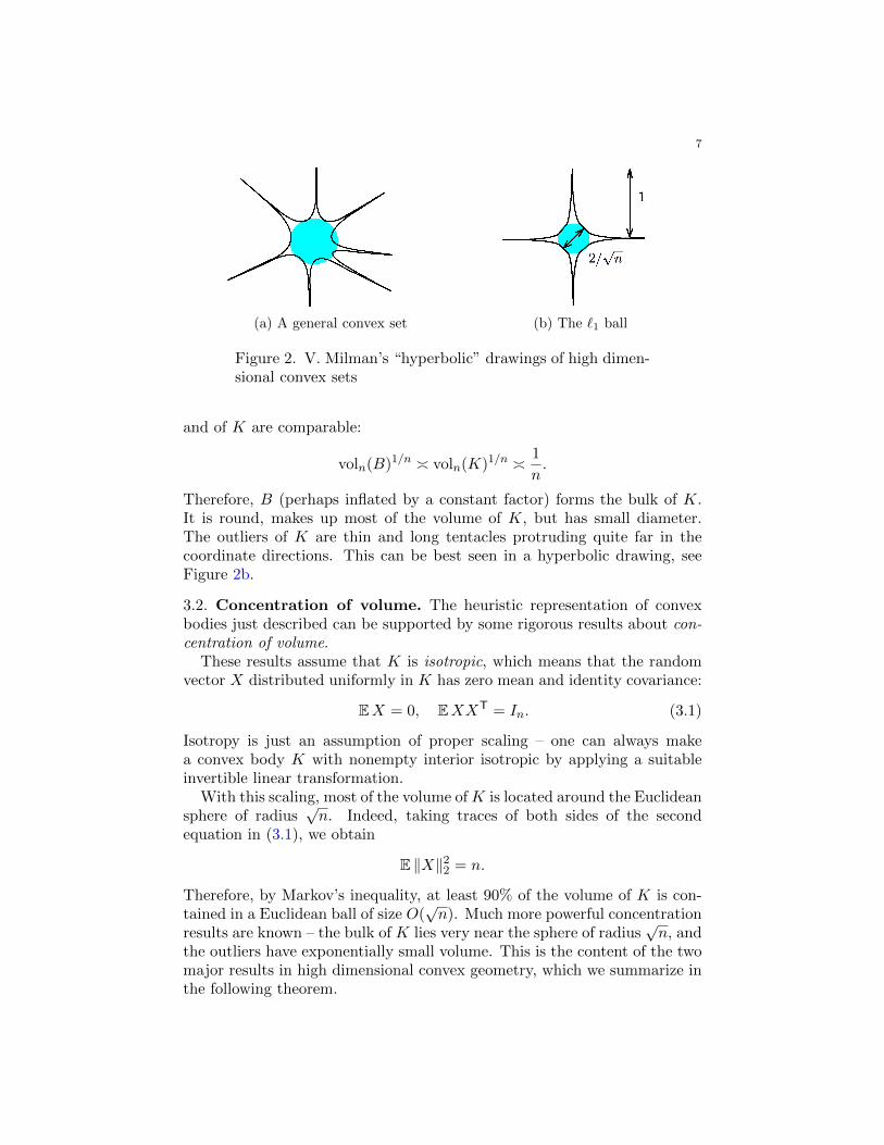
If K is properly scaled, the bulk usually looks like a Euclidean ball. Theoutliers look like thin, long tentacles. This is best seen on Figure 2a, whichdepicts V. Milman’s vision of high dimensional convex sets [48]. This picturedoes not look convex, and there is a good reason for this. The volume inhigh dimensions scales differently than in low dimensions – dilating of aset by the factor 2 increases its volume by the factor 2n. This is why it isnot surprising that the tentacles contain exponentially less volume than thebulk. Such behavior is best seen if a picture looks “hyperbolic”. Althoughnot convex, pictures like Figure 2 more accurately reflect the distribution ofvolume in higher dimensions.

Example 3.1 (The `1 ball). To illustrate this heuristic on a concrete example,consider the set

K = Bn1 = x ∈ Rn : ‖x‖1 ≤ 1,

i.e. the unit `1-ball in Rn. The inscribed Euclidean ball in K, which we willdenote by B, has diameter 2/

√n. One can then check that volumes of B

7

(a) A general convex set (b) The `1 ball

Figure 2. V. Milman’s “hyperbolic” drawings of high dimen-sional convex sets

and of K are comparable:

voln(B)1/n voln(K)1/n 1

n.

Therefore, B (perhaps inflated by a constant factor) forms the bulk of K.It is round, makes up most of the volume of K, but has small diameter.The outliers of K are thin and long tentacles protruding quite far in thecoordinate directions. This can be best seen in a hyperbolic drawing, seeFigure 2b.

3.2. Concentration of volume. The heuristic representation of convexbodies just described can be supported by some rigorous results about con-centration of volume.

These results assume that K is isotropic, which means that the randomvector X distributed uniformly in K has zero mean and identity covariance:

EX = 0, EXXT = In. (3.1)

Isotropy is just an assumption of proper scaling – one can always makea convex body K with nonempty interior isotropic by applying a suitableinvertible linear transformation.

With this scaling, most of the volume ofK is located around the Euclideansphere of radius

√n. Indeed, taking traces of both sides of the second

equation in (3.1), we obtain

E ‖X‖22 = n.

Therefore, by Markov’s inequality, at least 90% of the volume of K is con-tained in a Euclidean ball of size O(

√n). Much more powerful concentration

results are known – the bulk of K lies very near the sphere of radius√n, and

the outliers have exponentially small volume. This is the content of the twomajor results in high dimensional convex geometry, which we summarize inthe following theorem.

8 ROMAN VERSHYNIN

Theorem 3.2 (Distribution of volume in high-dimensional convex sets).Let K be an isotropic convex subset of Rn, and let X be a random vectoruniformly distributed in K. Then the following is true:

1. (Concentration of volume) For every t ≥ 1, one has

P‖X‖2 > t

√n≤ exp(−ct

√n).

2. (Thin shell) For every ε ∈ (0, 1), one has

P∣∣∣‖X‖2 −√n∣∣∣ > ε

√n≤ C exp(−cε3n1/2).

Here and later in this paper, C, c denote positive absolute constants.

The concentration part of Theorem 3.2 is due to G. Paouris [51]; see [1] foran alternative and shorter proof. The thin shell part is an improved versionof a result of B. Klartag [35], which is due to O. Guedon and E. Milman[30].

3.3. Low dimensional random sections. The intuition about bulk andoutliers of high dimensional convex sets K can help us to understand whatrandom sections of K should look like. Suppose E is a random subspace ofRn with fixed dimension d, i.e. E is drawn at random from the Grassmanianmanifold Gn,d according to the Haar measure. What does the section K∩Elook like on average?

If d is sufficiently small, then we should expect E to pass through thebulk of K and miss the outliers, as those have very small volume. Thus, ifthe bulk of K is a round ball,1 we should expect the section K ∩ E to be around ball as well; see Figure 3.

Figure 3. Random section of a high dimensional convex set

There is a rigorous result which confirms this intuition. It is known asDvoretzky’s theorem [20, 21], which we shall state in the form of V. Milman

1This intuition is a good approximation to truth, but it should to be corrected. Whileconcentration of volume tells us that the bulk is contained in a certain Euclidean ball (andeven in a thin spherical shell), it is not always true that the bulk is a Euclidean ball (orshell); a counterexample is the unit cube [−1, 1]n. In fact, the cube is the worst convexset in the Dvoretzky theorem, which we are about to state.

9

[45]; expositions of this result can be found e.g. in [53, 22]. Dvoretzky-Milman’s theorem has laid a foundation for the early development of asymp-totic convex geometry. Informally, this result says that random sections ofK of dimension d ∼ log n are round with high probability.

Theorem 3.3 (Dvoretzky’s theorem). Let K be an origin-symmetric convexset in Rn such that the ellipsoid of maximal volume contained in K is theunit Euclidean ball Bn

2 . Fix ε ∈ (0, 1). Let E be a random subspace ofdimension d = cε−2 log n drawn from the Grassmanian Gn,d according tothe Haar measure. Then there exists R ≥ 0 such that with high probability(say, 0.99) we have

(1− ε)B(R) ⊆ K ∩ E ⊆ (1 + ε)B(R).

Here B(R) is the centered Euclidean ball of radius R in the subspace E.

Several important aspects of this theorem are not mentioned here – inparticular how, for a given convex set K, to compute the radius R and thelargest dimension d of round sections of K. These aspects can be found inmodern treatments of Dvoretzky theorem such as [53, 22].

3.4. High dimensional random sections? Dvoretzky’s Theorem 3.3 de-scribes the shape of low dimensional random sections K∩E, those of dimen-sions d ∼ log n. Can anything be said about high dimensional sections, thosewith small codimension? In this more difficult regime, we can no longer ex-pect such sections to be round. Instead, as the codimension decreases, therandom subspace E becomes larger and it will probably pick more and moreof the outliers (tentacles) of K. The shape of such sections K ∩E is difficultto describe.

Nevertheless, it turns out that we can accurately predict the diameter ofK∩E. A bound on the diameter is known in asymptotic convex geometry asthe low M∗ estimate, or M∗ bound. We will state this result in Section 3.6and prove it in Section 5. For now, let us only mention that M∗ bound isparticularly attractive in applications as it depends only on two parameters– the codimension of E and a single geometric quantity, which informallyspeaking, measures the size of the bulk of K. This geometric quantity iscalled the mean width of K. We will pause briefly to discuss this importantnotion.

3.5. Mean width. The concept of mean width captures important geo-metric characteristics of sets in Rn. One can mentally place it in the samecategory as other classical geometric quantities like volume and surface area.

Consider a bounded subset K in Rn. (The convexity requirement will notbe imposed from now on.) The width of K in the direction of a given unitvector η ∈ Sn−1 is defined as the width of the smallest slab between twoparallel hyperplanes with normals η that contains K; see Figure 4.

10 ROMAN VERSHYNIN

Figure 4. Width of K in the direction of η

Analytically, we can express the width in the direction of η as

supu∈K〈η,u− v〉 = sup

z∈K−K〈η, z〉 ,

where K −K = u − v : u,v ∈ K is the Minkowski sum of K and −K.Averaging over η uniformly distributed on the sphere Sn−1, we can definethe spherical mean width of K:

w(K) := E supz∈K−K

〈η, z〉 .

It will be convenient to replace the spherical random vector η ∼ Unif(Sn−1)by the standard Gaussian random vector g ∼ N(0, In); the advantage is thatg has independent coordinates while η does not.

Definition 3.4 (Gaussian mean width). The Gaussian mean width of abounded subset K of Rn is defined as

w(K) := E supu∈K−K

〈g,u〉 , (3.2)

where g ∼ N(0, In) is a standard Gaussian random vector in Rn. We willoften refer to Gaussian mean width as simply the mean width.

3.5.1. Simple properties of mean width. Observe first that the Gaussianmean width is about

√n times larger than the spherical mean width. To see

this, using rotation invariance we realize η as η = g/‖g‖2. Next, we recallthat the direction and magnitude of a standard Gaussian random vector areindependent, so η is independent of ‖g‖2. It follows that

w(K) = E ‖g‖2 · w(K).

Further, the factor E ‖g‖2 is of order√n; this follows, for example, from

known bounds on the χ2 distribution:

c√n ≤ E ‖g‖2 ≤

√n (3.3)

where c > 0 is an absolute constant. Therefore, the Gaussian and sphericalversions of mean width are equivalent (up to scaling factor

√n), so it is

mostly a matter of personal preference which version to work with. In thispaper, we will mostly work with the Gaussian version.

Proposition 3.5. The mean width is invariant under translations, orthog-onal transformations, and taking convex hulls.

11

Especially useful is the last property, which states that

w(conv(K)) = w(K). (3.4)

This property will come handy later, when we consider convex relaxationsof optimization problems.

3.5.2. Computing mean width on examples. Let us illustrate the notion ofmean width on some simple examples.

Example 3.6. If K is the unit Euclidean ball Bn2 or sphere Sn−1, then

w(K) = E ‖g‖2 ≤√n

and also w(K) ≥ c√n, by (3.3).

Example 3.7. Let K is a subset of Bn2 and it has linear algebraic dimension

d. Then K lies in a d-dimensional unit Euclidean ball, so as before we have

w(K) ≤√d.

Example 3.8. Let K is a finite subset of Bn2 . Then

w(K) ≤ C√

log |K|.This follows from a known and simple computation of the expected maxi-mum of k = |K| Gaussian random variables.

Example 3.9 (Sparsity). Let K consist of all unit s-sparse vectors in Rn –those with at most s non-zero coordinates:

K = x ∈ Rn : ‖x‖2 = 1, ‖x‖0 ≤ s.Here ‖x‖0 denotes the number of non-zero coordinates of x. A simple com-putation (see e.g. [56, Lemma 2.3]) shows that

c√s log(n/s) ≤ w(K) ≤ C

√s log(n/s).

Example 3.10 (Low rank). Let K consist of d1 × d2 matrices with unitFrobeinus norm and rank at most r:

K = X ∈ Rd1×d2 : ‖X‖F = 1, rank(X) ≤ r.We will see in Proposition 10.4,

w(K) ≤ C√r(d1 + d2).

3.5.3. Computing mean width algorithmically. Can we estimate the meanwidth of a given set K fast and accurately? Gaussian concentration ofmeasure (see [53, 40, 39]) implies that, with high probability, the randomvariable

w(K, g) = supu∈K−K

〈g,u〉

is close to its expectation w(K). Therefore, to estimate w(K), it is enoughto generate a single realization of a random vector g ∼ N(0, In) and computew(K, g); this should produce a good estimator of w(K).

12 ROMAN VERSHYNIN

Since we can convexify K without changing the mean width by Propo-sition 3.5, computing this estimator is a convex optimization problem (andoften even a linear problem if K is a polytope).

3.5.4. Computing mean width theoretically. Finding theoretical estimates onthe mean width of a given set K is a non-trivial problem. It has been ex-tensively studied in the areas of probability in Banach spaces and stochasticprocesses.

Two classical results in the theory of stochastic processes – Sudakov’sinequality (see [40, Theorem 3.18]) and Dudley’s inequality (see [40, Theo-rem 11.17]) – relate the mean width to the metric entropy of K. Let N(K, t)denote the smallest number of Euclidean balls of radius t whose union coversK. Usually N(K, t) is referred to as a covering number of K, and logN(K, t)is called the metric entropy of K.

Theorem 3.11 (Sudakov’s and Dudley’s inequalities). For any boundedsubset K of Rn, we have

c supt>0

t√

logN(K, t) ≤ w(K) ≤ C∫ ∞

0

√logN(K, t) dt.

The lower bound is Sudakov’s inequality and the upper bound is Dudley’sinequality.

Neither Sudakov’s nor Dudley’s inequality are tight for all sets K. Amore advanced method of generic chaining produces a tight (but also morecomplicated) estimate of the mean width in terms of majorizing measures;see [64].

Let us only mention some other known ways to control mean width. Insome cases, comparison inequalities for Gaussian processes can be useful,especially Slepian’s and Gordon’s; see [40, Section 3.3]. There is also acombinatorial approach to estimating the mean width and metric entropy,which is based on VC-dimension and its generalizations; see [41, 44].

3.5.5. Mean width and Gaussian processes. The theoretical tools of estimat-ing mean width we just mentioned, including Sudakov’s, Dudley’s, Slepian’sand Gordon’s inequalities, have been developed in the context of stochasticprocesses. To see the connection, consider the Gaussian random variablesGu = 〈g,u〉 indexed by points u ∈ Rn. The collection of these random vari-ables (Gu)u∈K−K forms a Gaussian process, and the mean width measuresthe size of this process:

w(K) = E supu∈K−K

Gu.

In some sense, any Gaussian process can be approximated by a processof this form. We will return to the connection between mean width andGaussian processes in Section 5 where we prove the M∗ bound.

13

3.5.6. Mean width, complexity and effective dimension. In the context ofstochastic processes, Gaussian mean width (and its non-gaussian variants)play an important role in statistical learning theory. There it is more naturalto work with classes F of real-valued functions on 1, . . . , n than withgeometric sets K ⊆ Rn. (We identify a vector in Rn with a function on1, . . . , n.) The Gaussian mean width serves as a measure of complexity ofa function class in statistical learning theory, see [42]. It is sometimes calledGaussian complexity and is usually denoted γ2(F).

To get a better feeling of mean width as complexity, assume that K liesin the unit Euclidean ball Bn

2 . The square of the mean width, w(K)2,may be interpreted as the effective dimension of K. By Example 3.7, theeffective dimension is always bounded by the linear algebraic dimension.However, unlike algebraic dimension, the effective dimension is robust – asmall perturbation of K leads to a small change in w(K)2.

3.6. Random sections of small codimension: M∗ bound. Let us re-turn to the problem we posed in Section 3.4 – bounding the diameter ofrandom sections K ∩ E where E is a high-dimensional subspace. The fol-lowing important result in asymptotic convex geometry gives a good answerto this question.

Theorem 3.12 (M∗ bound). Let K be a bounded subset of Rn. Let E be arandom subspace of Rn of a fixed codimension m, drawn from the Grassma-nian Gn,n−m according to the Haar measure. Then

Ediam(K ∩ E) ≤ Cw(K)√m

.

We will prove a stronger version of this result in Section 5. The firstvariant of M∗ bound was found by V. Milman [46, 47]; its present form isdue to A. Pajor and N. Tomczak-Jaegermann [52]; an alternative argumentwhich yields tight constants was given by Y. Gordon [28]; an exposition ofM∗ bound can be found in [53, 40].

To understand the M∗ bound better, it is helpful to recall from Sec-tion 3.5.1 that w(K)/

√n is equivalent to the spherical mean width of K.

Heuristically, the spherical mean width measures the size of the bulk of K.For subspaces E of not very high dimension, where m = Ω(n), the M∗

bound states that the size of the random section K ∩ E is bounded bythe spherical mean width of K. In other words, subspaces E of proportionaldimension passes through the bulk of K and ignores the outliers (“tentacles”),just as Figure 3 illustrates. But when the dimension of the subspace E growstoward n (so the codimension m becomes small), the diameter of K∩E also

grows by a factor of√n/m. This gives a precise control of how E in this

case interferes with the outliers of K.

14 ROMAN VERSHYNIN

4. From geometry to estimation: linear observations

Having completed the excursion into geometry, we can now return to thehigh-dimensional estimation problems that we started to discuss in Section 2.To recall, our goal is to estimate an unknown vector

x ∈ K ⊆ Rn

that lies in a known feasible set K, from a random observation vector

y = (y1, . . . , ym) ∈ Rm,whose coordinates yi are random i.i.d. observations of x.

So far, we have not been clear about possible distributions of the ob-servations yi. In this section, we will study perhaps the simplest model –Gaussian linear observations. Consider i.i.d. standard Gaussian vectors

ai ∼ N(0, In)

and defineyi = 〈ai,x〉 , i = 1, . . . ,m.

Thus the observation vector y depends linearly on x. This is best expressedin a matrix form:

y = Ax.

Here A in an m×n Gaussian random matrix, which means that the entiresof A are i.i.d. N(0, 1) random variables; the vectors ai form the rows of A.

The interesting regime is when when the number of observations is smallerthan the dimension, i.e. when m < n. In this regime, the problem ofestimating x ∈ Rn from y ∈ Rm is ill posed. (In the complementary regime,where m ≥ n, the linear system y = Ax is well posed, so the solution istrivial.)

4.1. Estimation based on M∗ bound. Recall that we know two piecesof information about x:

1. x lies in a known random affine subspace x′ : Ax′ = y;2. x lies in a known set K.

Therefore, a good estimator of x can be obtained by picking any vector xfrom the intersection of these two sets; see Figure 5. Moreover, since justthese two pieces of information about x are available, such estimator is bestpossible in some sense.

Figure 5. Estimating x by any vector x in the intersectionof K with the affine subspace x′ : Ax′ = y

15

How good is such estimate? The maximal error is, of course, the distancebetween two farthest points in the intersection of K with the affine subspacex′ : Ax′ = y. This distance in turn equals the diameter of the section ofK by this random subspace. But this diameter is controlled by M∗ bound,Theorem 3.12. Let us put together this argument more rigorously.

In the following theorem, the setting is the same as above: K ⊂ Rn is abounded subset, x ∈ K is an unknown vector and y = Ax is the observationvector, where A is an m× n Gaussian matrix.

Theorem 4.1 (Estimation from linear observations: feasibility program).Choose x to be any vector satisfying

x ∈ K and Ax = y. (4.1)

Then

E supx∈K‖x− x‖2 ≤

Cw(K)√m

.

Proof. We apply the M∗ bound, Theorem 3.12, for the set K −K and thesubspace E = ker(A). Rotation invariance of Gaussian distribution impliesthat E is uniformly distributed in the Grassmanian Gn,n−m, as required bythe M∗ bound. Moreover, it is straightforward to check that w(K −K) ≤2w(K). It follows that

Ediam((K −K) ∩ E) ≤ Cw(K)√m

.

It remains to note that since x,x ∈ K and Ax = Ax = y, we have x− x ∈(K −K) ∩ E.

The argument we just described was first suggested by S. Mendelson,A. Pajor and N. Tomczak-Jaegermann [49].

4.2. Estimation as an optimization problem. Let us make one stepforward and replace the feasibility program (4.1) by a more flexible opti-mization program.

For this, let us make an additional (but quite mild) assumption that Khas non-empty interior and is star-shaped. Being star-shaped means thattogether with each point, the set K contains the segment joining that pointto the origin; in other words,

tK ⊆ K for all t ∈ [0, 1].

For such set K, let us revise the feasibility program (4.1). Instead of inter-secting a fixed set K with the affine subspace x′ : Ax′ = y, we may blowup K (i.e. consider a dilate tK with increasing t ≥ 0) until it touches thatsubspace. Choose x to be the touching point, see Figure 6. The fact thatK is star-shaped implies that x still belongs to K and (obviously) the affinesubspace; thus x satisfies the same error bound as in Theorem 4.1.

16 ROMAN VERSHYNIN

Figure 6. Estimating x by blowing up K until it touches theaffine subspace x′ : Ax′ = y

To express this estimator analytically, it is convenient to use the notionof Minkowski functional of K, which associates to each point x ∈ Rn anon-negative number ‖x‖K defined by the rule

‖x‖K = infλ > 0 : λ−1x ∈ K

.

A simple situation to think of is when K is an compact and origin-symmetricconvex set with non-empty interior; then ‖x‖K is a norm on Rn. The closedunit ball corresponding to this norm is K.

Let us now accurately state an optimization version of Theorem 4.1. It isvalid for an arbitrary bounded star-shaped set K with non-empty interior.

Theorem 4.2 (Estimation from linear observations: optimization program).Choose x to be a solution of the program

minimize ‖x′‖K subject to Ax′ = y. (4.2)

Then

E supx∈K‖x− x‖2 ≤

Cw(K)√m

.

Proof. It suffices to check that x ∈ K; the conclusion would then followfrom Theorem 4.1. Both x and x satisfy the linear constraint Ax′ = y.Therefore, by choice of x, we have

‖x‖K ≤ ‖x‖K ≤ 1;

the last inequality is nothing else than our assumption that x ∈ K. Thusx ∈ K as claimed.

4.3. Algorithmic aspects: convex programming. What does it take tosolve the optimization problem (4.2) algorithmically? If the feasible set Kis convex, then (4.2) is a convex program. In this case, to solve this problemnumerically, we may use one of the array of convex solvers. Further, if K is apolytope, then (4.2) can be cast as a linear program, which widens an arrayof algorithmic possibilities even further. For a quick preview, let us mentionthat examples of the latter kind will be discussed in detail in Section 7,where we will use K to enforce sparsity. We will thus choose K to be aball of `1 norm in Rn, so the program (4.2) will minimize ‖x′‖1 subject toAx′ = y. This is a typical linear program in the area of compressed sensing.

If K is not convex, then we can convexify it, thereby replacing K withits convex hull conv(K). Convexification does not change the mean width,

17

according to the remarkable property (3.4). Therefore, the generally non-convex problem (4.2) can be relaxed to the convex program

minimize ‖x′‖conv(K) subject to Ax′ = y, (4.3)

without compromising the guarantee of estimation stated in Theorem 4.2.The solution x of the convex program (4.3) still satisfies

E supx∈K‖x− x‖2 ≤

Cw(K)√m

.

Summarizing, we see that in any case, whether K is convex or not, theestimation problem reduces to solving an algorithmically tractable convexprogram. Of course, for this one needs to be able to compute ‖z‖conv(K)

algorithmically for a given vector z ∈ Rn. This is possible for many (butnot all) feasible sets K.

4.4. Information-theoretic aspects: effective dimension. If we fix adesired error level, for example if we aim for

E supx∈K‖x− x‖2 ≤ 0.01,

thenm ∼ w(K)2

observations will suffice. The implicit constant factor here is determined bythe desired error level.

Notice that this result is uniform, in the sense that with high probabilityin A (which determines the observation model) the estimation is accuratesimultaneously for all vectors x ∈ K.

The square of the mean width, w(K)2, can be thought of an effectivedimension of the feasible set K, as we pointed out in Section 3.5.6.

We can summarize our findings as follows.

Using convex programming, one can estimate a vector x ina general feasible set K from m random linear observations.A sufficient number of observations m is the same as theeffective dimension of K (the mean width squared), up to aconstant factor.

5. High dimensional sections: proof of a general M∗ bound

Let us give a quick proof of the M∗ bound, Theorem 3.12. In fact, withoutmuch extra work we will be able to derive a more general result from [55].First, it would allow us to treat noisy observations of the form y = Ax+ ν.Second, it will be generalizable for non-gaussian observations.

Theorem 5.1 (General M∗ bound). Let T be a bounded subset of Rn. LetA be an m × n Gaussian random matrix (with i.i.d. N(0, 1) entries). Fixε ≥ 0 and consider the set

Tε :=u ∈ T :

1

m‖Au‖1 ≤ ε

. (5.1)

18 ROMAN VERSHYNIN

Then

E supu∈Tε

‖u‖2 ≤√

2π

mE supu∈T| 〈g,u〉 |+

√π

2ε, (5.2)

where g ∼ N(0, In) is a standard Gaussian random vector in Rn.

To see that this result contains the classical M∗ bound, Theorem 3.12,we can apply it for T = K −K, ε = 0, and identify ker(A) with E. In thiscase,

Tε = (K −K) ∩ E.It follows that Tε ⊇ (K∩E)−(K∩E), so the left hand side in (5.2) is boundedbelow by diam(K∩E). The the right hand side in (5.2) by symmetry equals√

2π/mw(K). Thus, we recover Theorem 3.12 with C =√

2π.

Our proof of Theorem 5.1 will be based on two basic tools in the theoryof stochastic processes – symmetrization and contraction.

A stochastic process is simply a collection of random variables (Z(t))t∈Ton the same probability space. The index space T can be arbitrary; it maybe a time interval (such as in Brownian motion) or a subset of Rn (as willbe our case). To avoid measurability issues, we can assume that T is finiteby discretizing it if necessary.

Proposition 5.2. Consider a finite collection of stochastic processes Z1(t), . . . , Zm(t)indexed by t ∈ T . Let εi be independent symmetric Bernoulli random vari-ables, i.e. each εi independently takes values −1 and 1 with probabilities1/2. Then we have the following.

(i) (Symmetrization)

E supt∈T

∣∣∣ m∑i=1

[Zi(t)− EZi(t)

]∣∣∣ ≤ 2E supt∈T

∣∣∣ m∑i=1

εiZi(t)∣∣∣.

(ii) (Contraction)

E supt∈T

∣∣∣ m∑i=1

εi|Zi(t)|∣∣∣ ≤ E sup

t∈T

∣∣∣ m∑i=1

εiZi(t)∣∣∣.

Both statements are relatively easy to prove, and even in greater gener-ality. For example, taking the absolute values of Zi(t) in the contractionprinciple can be replaced by applying general Lipschitz functions. Proofs ofsymmetrization and contraction principles can be found in [40, Lemma 6.3]and [40, Theorem 4.12], respectively.

5.1. Proof of Theorem 5.1. The desired bound (5.2) would follow fromthe deviation inequality

E supu∈T

∣∣∣ 1

m

m∑i=1

| 〈ai,u〉 | −√

2

π‖u‖2

∣∣∣ ≤ 2√m

E supu∈T| 〈g,u〉 |. (5.3)

19

Indeed, if this inequality holds, then same is true is we replace T by thesmaller set Tε. But for u ∈ Tε, we have 1

m

∑mi=1 | 〈ai,u〉 | = 1

m‖Au‖1 ≤ ε,and the bound (5.2) follows by triangle inequality.

The rotation invariance of Gaussian distribution implies that

E | 〈ai,u〉 | =√

2

π‖u‖2. (5.4)

Thus, using symmetrization and then contraction inequalities from Propo-sition 5.2, we can bound the left side in (5.3) by

2E supu∈T

∣∣∣ 1

m

m∑i=1

εi 〈ai,u〉∣∣∣ = 2E sup

u∈T

∣∣∣∣∣⟨

1

m

m∑i=1

εiai,u

⟩∣∣∣∣∣ . (5.5)

Here εi are independent symmetric Bernoulli random variables.Conditioning on εi and using rotation invariance, we see that the random

vector

g :=1√m

m∑i=1

εiai

has distribution N(0, In). Thus (5.5) can be written as

2√m

E supu∈T| 〈g,u〉 |.

This proves (5.3) and completes the proof of Theorem 5.1.

6. Consequences: estimation from noisy linear observations

Let us apply the general M∗ bound, Theorem 5.1, to estimation problems.This will be even more straightforward than our application of the standardM∗ bound in Section 4. Moreover, we will now be able to treat noisyobservations.

Like before, our goal is to estimate an unknown vector x that lies in aknown feasible set K ⊂ Rn, from a random observation vector y ∈ Rm. Thistime we assume that, for some known level of noise ε ≥ 0, we have

y = Ax+ ν,1

m‖ν‖1 =

1

m

m∑i=1

|νi| ≤ ε. (6.1)

Here A is an m× n Gaussian matrix as before. The noise vector ν may beunknown and have arbitrary structure. In particular ν may depend on A,so even adversarial errors are allowed.

The following result is a generalization of Theorem 4.1 for noisy observa-tions (6.1).

Theorem 6.1 (Estimation from noisy linear observations: feasibility pro-gram). Choose x to be any vector satisfying

x ∈ K and1

m‖Ax− y‖1 ≤ ε. (6.2)

20 ROMAN VERSHYNIN

Then

E supx∈K‖x− x‖2 ≤

√2π

(w(K)√m

+ ε

).

Proof. We apply the general M∗ bound, Theorem 5.1, for the set T = K−K,and with 2ε instead of ε. It follows that

E supu∈T2ε

‖u‖2 ≤√

2π

mE supu∈T2ε

| 〈g,u〉 |+√

2π ε ≤√

2π

(w(K)√m

+ ε

).

The last inequality should be clear once we replace T2ε by the larger setT = K −K and use the symmetry of T .

To finish the proof, it remains to check that

x− x ∈ T2ε. (6.3)

To prove this, first note that x,x ∈ K, so x − x ∈ K −K = T . Next, bytriangle inequality, we have

1

m‖A(x− x)‖1 =

1

m‖Ax− y + ν‖1 ≤

1

m‖Ax− y‖1 +

1

m‖ν‖1 ≤ 2ε.

The last inequality follows from (6.1) and (6.2). We showed that the vectoru = x − x satisfies both constraints that define T2ε in (5.1). Hence (6.3)holds, and the proof of the theorem is complete.

And similarly to Theorem 4.2, we can cast estimation as an optimization(rather than feasibility) program.

Theorem 6.2 (Estimation from noisy linear observations: optimizationprogram). Choose x to be a solution to the program

minimize ‖x′‖K subject to1

m‖Ax′ − y‖1 ≤ ε. (6.4)

Then

E supx∈K‖x− x‖2 ≤

√2π

(w(K)√m

+ ε

).

Proof. It suffices to check that x ∈ K; the conclusion would then followfrom Theorem 6.1. Note first that by choice of x we have 1

m‖Ax− y‖1 ≤ ε,and by assumption (6.1) we have 1

m‖Ax− y‖1 = 1m‖ν‖1 ≤ ε. Thus both x

and x satisfy the constraint in (6.4). Therefore, by choice of x, we have

‖x‖K ≤ ‖x‖K ≤ 1;

the last inequality is nothing else than our assumption that x ∈ K. Itfollows x ∈ K as claimed.

The remarks about algorithmic aspects of estimation made in Sections 4.3and 4.4 apply also to the results of this section. In particular, the estimationfrom noisy linear observations (6.1) can be formulated as a convex program.

21

7. Applications to sparse recovery and regression

Remarkable examples of feasible sets K with low complexity come fromthe notion of sparsity. Consider the set K of all unit s-sparse vectors in Rn.As we mentioned in Example 3.9, the mean width of K is

w(K) ∼ s log(n/s).

According to the interpretation we discussed in Section 4.4, this means thatthe effective dimension of K is of order s log(n/s). Therefore,

m ∼ s log(n/s)

observations should suffice to estimate any s-sparse vector in Rn. Resultsof this type form the core of compressed sensing, a young area of signalprocessing, see [16, 36, 12, 32].

In this section we consider a more general model, where an unknownvector x has a sparse representation in some dictionary.

We will specialize Theorem 6.2 to the sparse recovery problem. Theconvex program will in this case amount to minimizing the `1 norm of thecoefficients. We will note that the notion of sparsity can be relaxed toaccommodate approximate, or “effective”, sparsity. Finally, we will observethat the estimate x is most often unique and m-sparse.

7.1. Sparse recovery for general dictionaries. Let us fix a dictionaryof vectors d1, . . . ,dN ∈ Rn. The dictionary may be arbitrary and evenredundant, i.e. not linearly independent. The choice of a dictionary dependson the application; common examples include unions of orthogonal bases andmore generally tight frames (in particular, Gabor frames). See [15, 18, 11, 17]for an introduction to sparse recovery problems with general dictionaries.

Suppose an unknown vector x ∈ Rn is s-sparse in the dictionary di.This means that x can be represented as a linear combination of at most sdictionary elements, i. e.

x =

N∑i=1

αidi with at most s non-zero coefficients αi ∈ R. (7.1)

As in Section 6, our goal is to recover x from a noisy observation vectory ∈ Rm of the form

y = Ax+ ν,1

m‖ν‖1 =

1

m

m∑i=1

|νi| ≤ ε.

Recall that A is a known m×n Gaussian matrix, and and ν is an unknownnoise vector, which can have arbitrary structure (in particular, correlatedwith A).

Theorem 6.2 will quickly imply the following recovery result.

22 ROMAN VERSHYNIN

Theorem 7.1 (Sparse recovery: general dictionaries). Assume for normal-ization that all dictionary vectors satisfy ‖di‖2 ≤ 1. Choose x to be asolution to the convex program

minimize ‖α′‖1 such that x′ =N∑i=1

α′idi satisfies1

m‖Ax′ − y‖1 ≤ ε. (7.2)

Then

E ‖x− x‖2 ≤ C√s logN

m· ‖α‖2 +

√2π ε.

Proof. Consider the sets

K := conv±diNi=1, K := ‖α‖1 · K.

Representation (7.1) implies that x ∈ K, so it makes sense to apply Theo-rem 6.2 for K.

Let us first argue that the optimization program in Theorem 6.2 can bewritten in the form (7.2). Observe that we can replace ‖x′‖K by ‖x′‖Kin the optimization problem (6.4) without changing its solution. (This isbecause ‖x′‖K = ‖α‖1 · ‖x′‖K and ‖α‖1 is a constant value.) Now, bydefinition of K, we have

‖x′‖K = min‖α′‖1 : x′ =

N∑i=1

α′idi

.

Therefore, the optimization programs (6.4) and (7.2) are indeed equivalent.Next, to evaluate the error bound in Theorem 6.2, we need to bound the

mean width of K. The convexification property (3.4) and Example 3.8 yield

w(K) = ‖α‖1 · w(K) ≤ C‖α‖1 ·√

logN.

Putting this into the conclusion of Theorem 6.2, we obtain the error bound

E supx∈K‖x− x‖2 ≤

√2π C

√logN

m· ‖α‖1 +

√2π ε.

To complete the proof, it remains to note that

‖α‖1 ≤√s · ‖α‖2, (7.3)

since α is s-sparse, i.e. it has only s non-zero coordinates.

7.2. Remarkable properties of sparse recovery. Let us pause to lookmore closely at the statement of Theorem 7.1.

7.2.1. General dictionaries. Theorem 7.1 is very flexible with respect to thechoice of a dictionary di. Note that there are essentially no restrictions onthe dictionary. (The normalization assumption ‖di‖2 ≤ 1 can be dispensedof at the cost of increasing the error bound by the factor of maxi ‖di‖2.) Inparticular, the dictionary may be linearly dependent.

23

7.2.2. Effective sparsity. The reader may have noticed that the proof ofTheorem 7.1 used sparsity in a quite mild way, only through inequality(7.3). So the result is still true for vectors x that are approximately sparsein the dictionary. Namely, the Theorem 7.1 will hold if we replace the exactnotion of sparsity (the number of nonzero coefficients) by the the moreflexible notion of effective sparsity, defined as

effective sparsity(α) := (‖α‖1/‖α‖2)2.

It is now clear how to extend sparsity in a dictionary (7.1) to approximatesparsity. We can say that a vector x is effectively s-sparse in a dictionarydi if it can be represented as x =

∑Ni=1 αidi where the coefficient vector

a = (α1, . . . , αN ) is effectively s-sparse.The effective sparsity is clearly bounded by the exact sparsity, and it is

robust with respect to small perturbations.

7.2.3. Linear programming. The convex programs (7.2) and (7.5) can bereformulated. This can be done by introducing new variables u1, . . . , uN ;instead of minimizing ‖α′‖1 in (7.2), we can equivalently minimize the linear

function∑N

i=1 ui subject to the additional linear constraints −ui ≤ α′i ≤ ui,i = 1, . . . , N . In a similar fashion, one can replace the convex constraint1m‖Ax

′ − y‖1 ≤ ε in (7.2) by n linear constraints.

7.2.4. Estimating the coefficients of sparse representation. It is worthwhileto notice that as a result of solving the convex recovery program (7.2), weobtain not only an estimate x of the vector x, but also an estimate α of thecoefficient vector in the representation x =

∑αidi. However, only x can be

estimated accurately; it should be clear that α can not be estimated by anymethod if the dictionary di is redundant (i.e. linearly dependent).

7.2.5. Sparsity of solution. The solution of the sparse recovery problem (7.2)may bot be exact in general, i.e. when x 6= x. This can be due to severalfactors – the generality of the dictionary, approximate (rather than exact)sparsity of x in the dictionary, or the noise ν in the observations. But even inthis general situation, the solution x is still m-sparse, in all but degeneratecases.

Proposition 7.2 (Sparsity of solution). Assume that a given convex recov-ery program (7.2) has a unique solution α for the coefficient vector. Thenα is m-sparse, and consequently x is m-sparse in the dictionary di. Thisis true even in presence of noise in observations, and even when no sparsityassumptions on x are in place.

Proof. The result follows by simple dimension considerations. First notethat the constraint on α′ in the optimization problem (7.2) can be writtenin the form

1

m‖ADα′ − y‖1 ≤ ε, (7.4)

24 ROMAN VERSHYNIN

where D is the n×N matrix whose columns are the dictionary vectors di.Since matrix AD has dimensions m × N , the constraint defines a cylinderin RN whose infinite directions are formed by the kernel of AD, which hasdimension at least N −m. Moreover, this cylinder is a polytope (due to the`1 norm defining it), so it has no faces of dimension smaller than N −m.

On the other hand, the level sets of the objective function ‖α′‖1 arealso polytopes; they are dilates of the unit `1 ball. The solution α of theoptimization problem (7.2) is thus a point in RN where the smallest dilateof the `1 ball touches the cylinder. The uniqueness of solution means thata touching point is unique. This is illustrated in Figure 7.

Figure 7. Illustration for the proof of Proposition 7.2. Thepolytope on the left represents a level set of the `1 ball. Thecylinder on the right represents the vectors α′ satisfying theconstraint (7.4). The two polytopes touch at point α.

Consider the faces of these two polytopes of smallest dimensions that con-tain the touching point; we may call these the touching faces. The touchingface of the cylinder has dimension at least N − m, as all of its faces do.Then the touching face of the `1 ball must have dimension at most m, oth-erwise the two touching faces would intersect by more than one point. Thistranslates into the m-sparsity of the solution α, as claimed.

7.2.6. Uniqueness of solution. In view of Proposition 7.2, we can ask whenthe solution α of the convex program (7.2) is unique. This does not alwayshappen; for example this fails if d1 = d2.

We can get around this problem by making an arbitrarily small genericperturbation of the dictionary elements, such as adding a small independentGaussian vector to each di. Then one can see that the solution α (andtherefore x as well) are unique almost surely. Invoking Proposition 7.2 wesee that x is m-sparse in the perturbed dictionary.

Note that we do not need the dictionary di to be linearly independent inorder for this to happen; the dictionary will always be dependent if N > n.

7.3. Sparse recovery for the canonical dictionary. Let us illustrateTheorem 7.1 for the simplest example of a dictionary – the canonical basisof Rn:

dini=1 = eini=1.

25

In this case, our assumption is that an unknown vector x ∈ Rn is s-sparsein the usual sense, meaning that x has at most s non-zero coordinates, oreffectively s-sparse as in Section 7.2.2. Theorem 7.1 then reads as follows.

Corollary 7.3 (Sparse recovery). Choose x to be a solution to the convexprogram

minimize ‖x′‖1 subject to1

m‖Ax′ − y‖1 ≤ ε. (7.5)

Then

E ‖x− x‖2 ≤ C√s log n

m· ‖x‖2 +

√2π ε.

Sparse recovery results like Corollary 7.3 form the core of the area ofcompressed sensing, see [16, 36, 12, 32].

In the noiseless case (ε = 0) and for sparse (rather then effectively sparse)vectors, one may even hope to recover x exactly, meaning that x = x withhigh probability. Conditions for exact recovery are now well understoodin compressed sensing. We will discuss some exact recovery problems inSection 9.

We can summarize Theorem 7.1 and the discussion around it as follows.

Using linear programming, one can approximately recover avector x that is s-sparse (or effectively s-sparse) in a gen-eral dictionary of size N , from m ∼ s logN random linearobservations.

7.4. Application: linear regression with constraints. The noisy es-timation problem (6.1) is equivalent to linear regression with constraints.So in this section we will translate the story into the statistical language.We present here just one class of examples out of a wide array of statisticalproblems; we refer the reader to [66] for a recent review of high dimensionalestimation problems from a statistical viewpoint.

Linear regression is a linear model of relationship between one dependentvariable and n explanatory variables. The problem is to find the best linearrelationship from a sample of p observations of dependent and explanatoryvariables. Linear regression is usually written as

y = Xβ + ν.

Here X is an n × p matrix which contains a sample of n observations of pexplanatory variables; y ∈ Rn represents a sample of n observations of thedependent variable; β ∈ Rp is a coefficient vector; ν ∈ Rn is a noise vector.We assume that X and y are known, while β and ν are unknown. Our goalis to estimate β.

We discussed a classical formulation of linear regression. In addition, weoften know, believe, or want to enforce some properties about the coefficientvector β, (for example, sparsity). We can express such extra information asthe assumption that

β ∈ K

26 ROMAN VERSHYNIN

where K ⊂ Rp is a known feasible set. Such problem may be called a linearregression with constraints.

The high dimensional estimation results we have seen so far can be trans-lated into the language of regression in a straightforward way. Let us dothis for Theorem 6.2; the interested reader can make a similar translationor other results.

We assume that the explanatory variables are independent N(0, 1), sothe matrix X has all i.i.d. N(0, 1) entries. This requirement may be toostrong in practice; however see Section 8 on relaxing this assumption. Thenoise vector ν is allowed have arbitrary structure (in particular, it can becorrelated with X). We assume that its magnitude is controlled:

1

n‖ν‖1 =

1

n

n∑i=1

|νi| ≤ ε

for some known noise level ε.

Theorem 7.4 (Linear regression with constraints). Choose β to be a solu-tion to the program

minimize ‖β′‖K subject to1

n‖Xβ′ − y‖1 ≤ ε.

Then

E supβ∈K‖β − β‖2 ≤

√2π

(w(K)√

n+ ε

).

8. Extensions from Gaussian to sub-gaussian distributions

So far, all our results were stated for Gaussian distributions. Let us showhow to relax this assumption. In this section, we will modify the proofof the M∗ bound, Theorem 5.1 for general sub-gaussian distributions, andindicate the consequences for the estimation problem. A result of this typewas proved in [49] with a much more complex argument.

8.1. Sub-gaussian random variables and random vectors. A system-atic introduction into sub-gaussian distributions can be found in Sections5.2.3 and 5.2.5 of [65]; here we briefly mention the basic definitions. Ac-cording to one of the several equivalent definitions, a random variable X issub-gaussian if

E exp(X2/ψ2) ≤ e.for some ψ > 0. The smallest ψ is called the sub-gaussian norm and isdenoted ‖X‖ψ2 .

The notion of sub-gaussian distribution transfers to higher dimensionsas follows. A random vector X ∈ Rn is called sub-gaussian if all one-dimensional marginals 〈X,u〉, u ∈ Rn, are sub-gaussian random variables.The sub-gaussian norm of X is defined as

‖X‖ψ2 := supu∈Sn−1

‖ 〈X,u〉 ‖ψ2 (8.1)

27

where, as before, Sn−1 denotes the Euclidean sphere in Rn. Recall also thatthe random vector X is called isotropic if

EXXT = In.

Isotropy is a scaling condition; any distribution in Rn which is not supportedin a low-dimensional subspace can be made isotropic by an appropriate lineartransformation.

8.2. M∗ bound for sub-gaussian distributions. Now we state and provea version of M∗ bound, Theorem 5.1, for general sub-gaussian distributions.It is a variant of a result from [49].

Theorem 8.1 (General M∗ bound for sub-gaussian distributions). Let Tbe a bounded subset of Rn. Let A be an m × n matrix whose rows ai arei.i.d., mean zero, isotropic and sub-gaussian random vectors in Rn. Chooseψ ≥ 1 so that

‖ai‖ψ2 ≤ ψ, i = 1, . . . ,m. (8.2)

Fix ε ≥ 0 and consider the set

Tε :=u ∈ T :

1

m‖Au‖1 ≤ ε

.

Then

E supu∈Tε

‖u‖2 ≤ Cψ4( 1√

mE supu∈Tε

| 〈g,u〉 |+ ε),

where g ∼ N(0, In) is a standard Gaussian random vector in Rn.

A proof of this result is an extension of the proof of the Gaussian M∗

bound, Theorem 5.1. Most of that argument generalizes to sub-gaussiandistributions in a standard way. The only non-trivial new step will be basedon the deep comparison theorem for sub-gaussian processes due to X. Fer-nique and M. Talagrand, see [64, Section 2.1]. Informally, the result statesthat any sub-gaussian process is dominated by a Gaussian process with thesame (or larger) increments.

Theorem 8.2 (Fernique-Talagrand’s comparison theorem). Let T be anarbitrary set.2 Consider a Gaussian random process (G(t))t∈T and a sub-gaussian random process (H(t))t∈T . Assume that EG(t) = EH(t) = 0 forall t ∈ T . Assume also that for some M > 0, the following incrementcomparison holds:3

‖H(s)−H(t)‖ψ2 ≤M (E ‖G(s)−G(t)‖22)1/2 for all s, t ∈ T.Then

E supt∈T

H(t) ≤ CM E supt∈T

G(t).

2We can assume T to be finite to avoid measurability complications, and then proceedby approximation; see e.g. [40].

3The increment comparison may look better if we replace the L2 norm in the right handside by ψ2 norm. Indeed, it is easy to see that ‖G(s)−G(t)‖ψ2 (E ‖G(s)−G(t)‖22)1/2.

28 ROMAN VERSHYNIN

This theorem is a combination of a result of X. Fernique [31] that boundsE supt∈T H(t) above by the so-called majorizing measure of T , and a result ofM. Talagrand [63] that bounds E supt∈T G(t) below by the same majorizingmeasure of T .

Proof of Theorem 8.1. Let us examine the proof of the Gaussian M∗ bound,Theorem 5.1, check where we used Gaussian assumptions, and try to accom-modate sub-gaussian assumptions instead.

The first such place is identity (5.4). We claim that a version of it stillholds for the sub-gaussian random vector a, namely

‖u‖2 ≤ C0ψ3 Ea | 〈a,u〉 | (8.3)

where C0 is an absolute constant.4

To check (8.3), we can assume that ‖u‖2 = 1 by dividing both sides by‖u‖2 if necessary. Then Z := 〈a,u〉 is sub-gaussian random variable, sinceaccording to (8.1) and (8.2), we have ‖Z‖ψ2 ≤ ‖a‖ψ2 ≤ ψ. Then, since sub-gaussian distributions have moments of all orders (see [65, Lemma 5.5]), we

have (EZ3)1/3 ≤ C1‖Z‖ψ2 ≤ C1ψ, where C1 is an absolute constant. Usingthis together with isotropy and Cauchy-Schwarz inequality, we obtain

1 = EZ2 = EZ1/2Z3/2 ≤ (EZ)1/2(EZ3)1/2 ≤ (EZ)1/2(C1ψ)3/2.

Squaring both sides implies (8.3), since we assumed that ‖u‖2 = 1.The next steps in the proof of Theorem 5.1 – symmetrization and contrac-

tion – go through for sub-gaussian distributions without change. So (5.5) isstill valid in our case.

Next, the random vector

h :=1√m

m∑i=1

εiai

is no longer Gaussian as in the proof of Theorem 5.1. Still, h is sub-gaussianwith

‖h‖ψ2 ≤ C2ψ (8.4)

due to the approximate rotation invariance of sub-gaussian distributions,see [65, Lemma 5.9].

In the last step of the argument, we need to replace the sub-gaussianrandom vector h by the Gaussian random vector g ∼ N(0, In), i.e. provean inequality of the form

E supu∈Tε

| 〈h,u〉 | . E supu∈Tε

| 〈g,u〉 |.

4We should mention that a reverse inequality also holds: by isotropy, one hasEa | 〈a,u〉 | ≤ (Ea 〈a,u〉2)1/2 = ‖u‖2. However, this inequality will not be used in theproof.

29

This can be done by applying the comparison inequality of Theorem 8.2 forthe processes

H(u) = 〈h,u〉 and G(u) = 〈g,u〉 , u ∈ T ∪ (−T ).

To check the increment inequality, we can use (8.4), which yields

‖H(u)−H(v)‖ψ2 = ‖ 〈h,u− v〉 ‖ψ2 ≤ ‖h‖ψ2 ‖u− v‖2 ≤ C2ψ ‖u− v‖2.On the other hand,

(E ‖G(u)−G(v)‖22)1/2 = ‖u− v‖2.Therefore, the increment inequality in Theorem 8.2 holds with M = C2ψ.It follows that

E supu∈T∪(−T )

〈h,u〉 ≤ C3ψ E supu∈T∪(−T )

〈g,u〉 .

This means that

E supu∈T| 〈h,u〉 | ≤ C3ψ E sup

u∈T| 〈g,u〉 |

as claimed.Replacing all Gaussian inequalities by their sub-gaussian counterparts

discussed above, we complete the proof just like in Theorem 5.1.

Remark 8.3 (Dependence on sub-gaussian norm). The dependence on ψ inTheorem 8.1 is not optimal. To make the argument transparent, we havenot tried to optimize this dependence; the interested reader is encouragedto do so.

8.3. Estimation from sub-gaussian linear observations. It is now straight-forward to generalize all recovery results we developed before from Gaussianto sub-gaussian observations. So our observations are now

yi = 〈ai, x〉+ νi, i = 1, . . . ,m

where ai are i.i.d., mean zero, isotropic and sub-gaussian random vectorsin Rn. As in Theorem 8.1, we control the sub-gaussian norm with theparameter ψ > 1, choosing it so that

‖ai‖ψ2 ≤ ψ, i = 1, . . . ,m.

We can write observations in the matrix form as in (6.1), i.e.

y = Ax+ ν,

where A is the m × n matrix with rows ai. As before, we assume somecontrol on the error:

1

m‖ν‖1 =

1

m

m∑i=1

|νi| ≤ ε.

Let us state a version of Theorem 6.1 for sub-gaussian observations. Itsproof is the same, except we use the sub-gaussian M∗ bound, Theorem 8.1where previously a Gaussian M∗ bound was used.

30 ROMAN VERSHYNIN

Theorem 8.4 (Estimation from sub-gaussian observations). Choose x tobe any vector satisfying

x ∈ K and1

m‖Ax− y‖1 ≤ ε.

Then

E supx∈K‖x− x‖2 ≤ Cψ4

(w(K)√m

+ ε

).

In a similar fashion, one can generalize all other estimation results estab-lished before to sub-gaussian observations. We leave this to the interestedreader.

9. Exact recovery

In some situations, one can hope to estimate vector x ∈ K from y exactly,without any error. Such results form the core of the area of compressedsensing. [16, 36, 32]. Here we will present an approach to exact recoverybased on Y. Gordon’s “escape through a mesh” theorem [28]. This argumentgoes back to [60] for the set of sparse vectors; it was put in a general contextin [13].

We will work here with Gaussian observations

y = Ax,

where A is an m × n Gaussian random matrix. This is the same model aswe considered in Section 4.

9.1. Exact recovery condition and the descent cone. When can x beinferred from y exactly? Recall that we only know two things about x –that it lies in the feasible set K and in the affine subspace

Ex := x′ : Ax′ = y.

This two pieces of information determine x uniquely if and only if these twosets intersect at the single point x:

K ∩ Ex = x. (9.1)

Notice that this situation would go far beyond theM∗ bound on the diameterof K ∩E (see Theorem 3.12) – indeed, in this case the diameter would equalzero!

How can this be possible? Geometrically, the exact recovery condition(9.1) states that the affine subspace Ex is tangent to the set K at the pointx; see Figure 8a for illustration.

This this condition is local. Assuming that K is convex for better un-derstanding, we see that the tangency condition depends on the shape ofK in an infinitesimal neighborhood of x, while the global geometry of K isirrelevant. So we would not lose anything if we replace K by the descent

31

(a) Exact recovery condition(9.1): affine subspace Ex is tan-gent to K at x

(b) Picture translated by −x:subspace ker(A) is tangent to de-scent cone D(K,x) at 0

Figure 8. Illustration of the exact recovery condition (9.1)

cone at point x, see Figure 8b. This set is formed by the rays emanatingfrom x into directions of points from K:

D(K,x) := t(z − x) : z ∈ K, t ≥ 0.Translating by −x, can we rewrite the exact recovery condition (9.1) as

(K − x) ∩ (Ex − x) = 0Reeplacing K−x by the descent cone (a bigger set) and noting that Ex−x =ker(A), we rewrite this again as

D(K,x) ∩ ker(A) = 0.The descent cone can be determined by its intersection with the unit sphere,i.e. by

S(K,x) := D(K,x) ∩ Sn−1 = z − x‖z − x‖2

: z ∈ K. (9.2)

Thus we arrive at the following equivalent form of the exact recovery con-dition (9.1):

S(K,x) ∩ ker(A) = ∅;

see Figure 8b for an illustration.

9.2. Escape through a mesh, and impications for exact recovery.It remains to understand under what conditions the random subspace kerAmisses a given subset S = S(K,x) of the unit sphere. There is a remarkablysharp result in asymptotic convex geometry that answers this question forgeneral subsets S. This is the theorem on escape through a mesh, which isdue to Y. Gordon [28]. Similarly to the other results we saw before, thistheorem depends on the mean width of S, defined as5

w(S) = E supu∈S〈g,u〉 , where g ∼ N(0, In).

5The only (minor) difference with our former definition (3.2) of the mean width is thatwe take supremum over S instead of S − S, so w(S) is a smaller quantity. The reason wedo not need to consider S − S because we already subtracted x in the definition of thedescent cone.

32 ROMAN VERSHYNIN

Theorem 9.1 (Escape through a mesh). Let S be a fixed subset of Sn−1.Let E be a random subspace of Rn of a fixed codimension m, drawn fromthe Grassmanian Gn,n−m according to the Haar measure. Assume that

w(S) <√m.

Then

S ∩ E = ∅with high probability, namely 1− 2.5 exp

[− (m/

√m+ 1− w(S))2/18

].

Applying this result for S = S(K,x) and E = ker(A), we conclude bythe argument above that the exact recovery condition (9.1) holds with highprobability if

m > w(S)2.

How can we algorithmically recover x in these circumstances? We cando the same as in Section 4.1, either using the feasibility program (4.1)or, better yet, the optimization program (4.2). The only difference is thatthe diameter of the intersection is now zero, so the recovery is exact. Thefollowing is an exact version of Theorem 4.2.

Theorem 9.2 (Exact recovery from linear observations). Choose x to be asolution of the program

minimize ‖x′‖K subject to Ax′ = y.

Assume that the number of observations satisfies

m > w(S)2 (9.3)

where S = S(K,x) is the spherical part of the descent cone of K, defined in(9.2). Then

x = x

with high probability (the same as in Theorem 9.1).

Note the familiar condition (9.3) on m which we have seen before, see e.g.Section 4.3. Informally, it states the following:

Exact recovery is possible when the number of measurementsexceeds the effective dimension of the descent cone.

Remarkably, the condition (9.3) does not have absolute constant factorswhich we had in results before.

9.3. Application: exact sparse recovery. Let us illustrate how Theo-rem 9.2 works for exact sparse recovery. Assume that x is s-sparse, i.e.it has at most s non-zero coefficients. For the feasible set, we can chooseK := ‖x‖1Bn

1 = x′ : ‖x′‖1 ≤ ‖x‖1. One can write down accurately anexpression for the descent cone, and derive a familiar bound on the meanwidth of S = S(K,x):

w(S) ≤ C√s log n;

33

see [60] for details. We plug this into Theorem 9.2, where we replace ‖x′‖Kin the optimization problem by the proportional quantity ‖x′‖1. This leadsto the following exact version of Corollary 7.3:

Theorem 9.3 (Exact sparse recovery). Assume that an unknown vectorx ∈ Rn is s-sparse. Choose x to be a solution to the convex program

minimize ‖x′‖1 subject to Ax′ = y.

Assume that the number of observations satisfies m > Cs log n. Then

x = x

with high probability, namely 1− 2.5e−m.

Due to the remarkable sharpness of Gordon’s theorem, one may hope toobtain sharp conditions on the number of observations m (without absoluteconstants). This was done in [19] for the sparse recovery problem, and morerecently in [3] for general feasible cones. The latter paper proves a variant ofGordon’s theorem with a slightly different (but still closely related) versionof mean width.

10. Low-rank matrix recovery and matrix completion

10.1. Background: matrix norms. The theory we developed so far con-cerns estimation of vectors in Rn. It should not be surprising that this theorycan also be applied for matrices. Matrix estimation problems were studiedrecently in particular in [8, 9, 34, 10, 59].

Let us recall some basic facts about matrices and their norms. We canidentify d1 × d2 matrices with vectors in Rd1×d2 . The `2 norm in Rd1×d2 isthen nothing else than Frobenius (or Hilbert-Schmidt) norm of matrices:

‖X‖F =( d1∑i=1

d2∑j=1

|Xij |2)1/2

.

The inner product in Rd1×d2 can be written in matrix form as follows:

〈X,Y 〉 = tr(XTY ).

Denote d = min(d1, d2). Let

s1(X) ≥ s2(X) ≥ · · · ≥ sd(X) ≥ 0

denote the singular values of X. Then Frobenius norm has the followingspectral representation:

‖X‖F =( d∑i=1

si(X)2)1/2

.

Recall also the operator norm of X, which is

‖X‖ = maxu∈Rn\0

‖Xu‖2‖u‖2

= maxi=1,...,d

si(X).

34 ROMAN VERSHYNIN

Finally, the nuclear norm of X is defined as

‖X‖∗ =d∑i=1

si(X).

Spectrally, i.e. on the level of singular values, the nuclear norm is aversion of `1 norm for matrices, the Frobenius norm is a version of `2 normfor matrices, and the operator norm is a version of `∞ norm for matrices.In particular, the following inequality holds:

‖X‖ ≤ ‖X‖F ≤ ‖X‖∗.

The reader should be able to derive many other useful inequalities in asimilar way, for example

‖X‖∗ ≤√

rank(X) · ‖X‖F , ‖X‖F ≤√

rank(X) · ‖X‖ (10.1)

and

〈X,Y 〉 ≤ ‖X‖ · ‖Y ‖∗. (10.2)

10.2. Low-rank matrix recovery. We are ready to formulate a matrixversion of the sparse recovery problem from Section 7. Our goal is to esti-mate an unknown d1 × d2 matrix X from m linear observations given by

yi = 〈Ai, X〉 , i = 1, . . . ,m. (10.3)

Here Ai are independent d1 × d2 Gaussian matrices with all i.i.d. N(0, 1)entries.

There are two natural matrix versions of sparsity. The first version is thesparsity of entries. We will be concerned with the other, spectral, type ofsparsity, where there are only a few non-zero singular values. This simplymeans that the matrix has low rank. So let us assume that the unknownmatrix X satisfies

rank(X) ≤ r (10.4)

for some fixed (and possibly unknown) r ≤ n.The following is a matrix version of Corollary 7.3; for simplicity we are

stating it in a noise-free setting (ε = 0).

Theorem 10.1 (Low-rank matrix recovery). Choose X to be a solution tothe convex program

minimize ‖X ′‖∗ subject to⟨Ai, X

′⟩ = yi, i = 1, . . . ,m. (10.5)

Then

E supX‖X −X‖F ≤ 4

√π

√r(d1 + d2)

m· ‖X‖F .

Here the supremum is taken over all d1 × d2 matrices X or rank at most r.

35

The proof of Theorem 10.1 will closely follow its vector prototype, thatof Theorem 7.1; we will just need to replace the `1 norm by the nuclearnorm. The only real difference will be in the computation of the mean widthof the unit ball of the nuclear norm. This computation will be based onY. Gordon’s bound on the operator norm of Gaussian random matrices, seeTheorem 5.32 in [65].

Theorem 10.2 (Gordon’s bound for Gaussian random matrices). Let G bean d1×d2 matrix whose entries are i.i.d. mean zero random variables. Then

E ‖G‖ ≤√d1 +

√d2.

Proposition 10.3 (Mean width of the unit ball of nuclear norm). Considerthe unit ball in the space of d1 × d2 matrices corresponding to the nuclearnorm:

B := X ∈ Rd1×d2 : ‖X‖∗ ≤ 1.Then

w(B) ≤ 2(√d1 +

√d2).

Proof. By definition and symmetry of B, we have

w(B) = E supX∈B−B

〈G,X〉 = 2E supX∈B

〈G,X〉 ,

where G is a d1 × d2 Gaussian random matrix with N(0, 1) entries. Usinginequality (10.2) and definition of B, we obtain we obtain

w(B) ≤ 2E supX∈B

‖G‖ · ‖X‖∗ ≤ 2E ‖G‖.

To complete the proof, it remains to apply Theorem 10.2.

Let us mention an immediate consequence of Proposition 10.3, althoughit will not be used in the proof of Theorem 10.1.

Proposition 10.4 (Mean width of the set of low-rank matrices). Let

D = X ∈ Rd1×d2 : ‖X‖F = 1, rank(X) ≤ r.Then

w(D) ≤ C√r(d1 + d2).

Proof of Proposition 10.4. The bound follows immediately from Proposi-tion 10.3 and the first inequality in (10.1), which implies thatD ⊂

√r·B.

Proof of Theorem 10.1. The argument is a matrix version of the proof ofTheorem 7.1. We consider the following subsets of d1 × d2 matrices:

K := X ′ : ‖X ′‖∗ ≤ 1, K := ‖X‖∗ · K.Then obviously X ∈ K, so it makes sense to apply Theorem 6.2 (with ε = 0)for K. It should also be clear that the optimization program in Theorem 6.2can be written in the form (10.5).

36 ROMAN VERSHYNIN

Applying Theorem 6.2, we obtain

E supX‖X −X‖F ≤

√2π · w(K)√

m.

Recalling the definition of K and using Proposition 10.3 to bound its meanwidth, we have

w(K) = w(K) · ‖X‖∗ ≤ 2√

2√d1 + d2 · ‖X‖∗.

It follows that

E supX‖X −X‖F ≤ 4

√π

√d1 + d2

m· ‖X‖∗.

It remains to use the low-rank assumption (10.4). According to the firstinequality in (10.1), we have

‖X‖∗ ≤√r‖X‖F .

This completes the proof of Theorem 10.1.

10.3. Low-rank matrix recovery: some extensions.

10.3.1. From exact to effective low rank. The exact low rank assumption(10.4) can be replaced by approximate low rank assumption. This is amatrix version of a similar observation about sparsity which we made inSection 7.2.2. Indeed, our argument shows that Theorem 10.1 will hold ifwe replace the rank by the more flexible effective rank, defined for a matrixX as

r(X) = (‖X‖∗/‖X‖F )2.

The effective rank is clearly bounded by the algebraic rank, and it is robustwith respect to small perturbations.

10.3.2. Noisy and sub-gaussian observations. Our argument makes it easyto allow noise in the observations (10.3), i.e. consider observations of theform yi = 〈Ai, X〉+ νi. We leave details to the interested reader.

Further, just like in Section 8, we can relax the requirement that Ai beGaussian random matrices, replacing it with a sub-gaussian assumption.Namely, it is enough to assume that the columns of Ai are i.i.d., mean zero,isotropic and sub-gaussian random vectors in Rd1 , with a common boundon the sub-gaussian norm. We again leave details to the interested reader.

We can summarize the results about low-rank matrix recovery as follows.

Using convex programming, one can approximately recovera d1 × d2 matrix which has rank (or effective rank) r, fromm ∼ r(d1 + d2) random linear observations.

To understand this number of observations better, note that it is of thesame order as the number of degrees of freedom in the set of d1×d2 matricesor rank r.

37

10.4. Matrix completion. Let us now consider a different, and perhapsmore natural, model of observations of matrices. Assume that we are givena small random sample of entries of an unknown matrix matrix X. Ourgoal is to estimate X from this sample. As before, we assume that X haslow rank. This is called a matrix completion problem, and it was extensivelystudied recently [8, 9, 34, 59].

We can not apply the previously developed theory for such observations.While sampling of entries is a linear operation, such observations are notGaussian or sub-gaussian (more accurately, we should say that the sub-gaussian norm of such observations is too large).

Nevertheless, it is possible able to derive a matrix completion result inthis setting. Our exposition will be based on a direct argument and simplefrom [57].

Let us formalize the process of sampling the entries of X. First, we fixthe average size m of the sample. Then we generate selectors δij ∈ 0, 1for each entry of X. Those are i.i.d. random variables with

E δij =m

d1d2=: p.

Our observations are given as the d1 × d2 matrix Y whose entries are

Yij = δijXij .

Therefore, the observations are randomly and independently sampled entriesof X along with the indices of these entries; the average sample size is fixedand equals m. We will require that

m ≥ d1 log d1, m ≥ d2 log d2. (10.6)

These restrictions ensure that, with high probability, the sample containsat least one entry from each row and each column of X (recall the classicalcoupon collector’s problem).

As before, we assume that

rank(X) ≤ r.

The next result that X can be estimated from Y using low-rank approxi-mation.

Theorem 10.5 (Matrix completion). Choose X to be best rank-r approxi-mation6 of p−1Y . Then

E1√d1d2

‖X −X‖F ≤ C√r(d1 + d2)

m‖X‖∞, (10.7)

where ‖X‖∞ = maxi,j |Xij |.

6Formally, consider the singular value decomposition p−1Y =∑i siuiv

Ti with non-

increasing singular values si. We define X by retaining the r leading terms of this decom-

position, i.e. X =∑ri=1 siuiv

Ti .

38 ROMAN VERSHYNIN

To understand the form of this estimate, note that the left side of (10.7)measures the average error per entry of X:

1√d1d2

‖X −X‖F =( 1

d1d2

d1∑i=1

d2∑j=1

|Xij −Xij |2)1/2

.

So, Theorem 10.5 allows to make the average error per entry arbitrarilysmaller than the maximal entry of the matrix. Such estimation succeedswith a sample of m ∼ r(d1 + d2) entries of X.

The proof of Theorem 10.5 will be based on a known bound on the op-erator norm of random matrices, which is more general than Y. Gordon’sTheorem 10.2. There are several ways to obtain general bounds; see [65]for a systematic treatment of this topic. We will use one such result due toY. Seginer [61].

Theorem 10.6 (Seginer’s bound for general random matrices). Let G be and1 × d2 matrix whose entries are i.i.d. mean zero random variables. Then

E ‖G‖ ≤ C(Emax

i‖Gi‖2 + Emax

j‖Gj‖2

)where the maxima are taken over all rows Gi and over all columns Gj of G,respectively.

Proof of Theorem 10.5. We shall first control the error in the operator norm.By triangle inequality,

‖X −X‖ ≤ ‖X − p−1Y ‖+ ‖p−1Y −X‖. (10.8)

Since X is the best rank-r approximation to p−1Y , and both X and X arerank-r matrices, the first term in (10.8) is bounded by the second term.Thus

‖X −X‖ ≤ 2‖p−1Y −X‖ =2

p‖Y − pX‖. (10.9)

The matrix Y − pX has independent mean zero entries, namely

(Y − pX)ij = (δij − p)Xij .

So we can apply Y. Seginer’s Theorem 10.6, which yields

E ‖Y − pX‖ ≤ C(Emaxi≤d1‖(Y − pX)i‖2 + Emax

j≤d2‖(Y − pX)j‖2

). (10.10)

It remains to bound the `2 norms of rows and columns of Y − PX. Letus do this for rows; a similar argument would control the columns. Since

‖(Y − pX)i‖22 =

d2∑j=1

(δij − p)2|Xij |2 ≤d2∑j=1

(δij − p)2 · ‖X‖∞,

39

this quantity can be bounded using concentration inequalities for sums of in-dependent random variables. In particular, we can use Bernstein’s inequality(see [6]), which yields

P

d2∑j=1

(δij − p)2 > pd2t

≤ exp(−cpd2t), t ≥ 2.

The first restriction in (10.6) guarantees that pd2 ≥ log d1. This enables usto use the union bound over i ≤ d1, which yields

Emaxi≤d1

[ d2∑j=1

(δij − p)2]1/2≤ C1pd2.

This translates into the following bound for the rows of Y − PX:

Emaxi≤d1‖(Y − pX)i‖2 ≤ C1

√pd2 ‖X‖∞.

Repeating this argument for columns and putting the two bounds into(10.10), we obtain

‖Y − pX‖ ≤ C2

√p(d1 + d2) ‖X‖∞.

Substituting into (10.9), we conclude that

‖X −X‖ ≤ C3

√d1 + d2

p‖X‖∞. (10.11)

It remains to pass to the Frobeinus norm. This is where we use the low

rank assumption on X. Since both X and X have ranks bounded by r, we

have rank(X−X) ≤ 2r. Then, according to the second inequality in (10.1),

‖X −X‖F ≤√

2r ‖X −X‖.

Combining this with (10.11) and recalling that p = m/(d1d2) by definition,we arrive at the desired bound (10.7).

Remark 10.7 (Noisy observations). One can easily extend Theorem 10.5 fornoisy sampling, where every observed entry of X is independently corruptedby a mean-zero noise. Formally, we assume that the entries of the observa-tion matrix Y are

Yij = δij(Xij + νij)

where νij are independent and mean zero random variables. Let us furtherassume that |νij | ≤M almost surely. Then a slight modification of the proofof Theorem 10.5 yields the following error bound:

E1√d1d2

‖X −X‖F ≤ C√r(d1 + d2)

m

(‖X‖∞ +M

).

We leave details to the interested reader.

40 ROMAN VERSHYNIN

11. Single-bit observations via hyperplane tessellations

It may perhaps be surprising that a theory of similar strength can bedeveloped for estimation problems with non-linear observations, in whichthe observation vector y ∈ Rm depends non-linearly on the unknown vectorx ∈ Rn.

In this and next sections we explore an example of extreme non-linearity– the one given by the sign function. in Section 13, we will extend the theoryto completely general non-linearities.

11.1. Single-bit observations. As before, our goal is to estimate an un-known vector x that lies in a known feasible set K ⊂ Rn, from a randomobservation vector y = (y1, . . . , ym) ∈ Rm. This time, we will work withsingle-bit observations yi ∈ −1, 1. So, we assume that

yi = sign 〈ai,x〉 , i = 1, . . . ,m, (11.1)

where ai are standard Gaussian random vectors, i.e. ai ∼ N(0, In). We canrepresent the model in a matrix form:

y = sign(Ax),

where A is an m × n Gaussian random matrix with rows ai, and whereour convention is that the sign function is applied to each coordinate of thevector Ax.

The single-bit model represents an extreme quantization of the linearmodel we explored before, where y = Ax. Only one bit is retained fromeach linear observation yi. Yet we hope to estimate x as accurately as if allbits were available.

The model of single-bit observations was first studied in this context in[7]. Our discussion will follow [55].

11.2. Hyperplane tessellations. Let us try to understand single-bit ob-servations yi from a geometric perspective. Each yi ∈ −1, 1 representsthe orientation of the vector x with respect to the hyperplane with normalai. There are m such hyperplanes. The observation vector y = (y1, . . . , ym)represents orientation of x with respect to all these hyperplanes.

Geometrically, the m hyperplanes induce a tessellation of Rn by cells.A cell is a set of points that have the same orientation with respect to allhyperplanes; see Figure 9. Knowing y is the same as knowing the cell wherex lies.

How can we estimate x? Recall that we know two pieces of informationabout x:

1. x lies in a known cell of the hyperplane tessellation;2. x lies in a known set K.

Therefore, a good estimator of x can be obtained by picking any vectorx from the intersection of these two sets. Moreover, since just these two

41

Figure 9. A tessellation of the feasible set K by hyperplanes.The cell containing x is highlighted.

pieces of information about x are available, such estimator is best possiblein some sense.

11.3. M∗ bound for random tessellations. How good is such estimate?The maximal error is of course the diameter of the intersection of the cellwith K. So in order to bound the error, we need to prove that this diameteris small.

Note that our strategy is parallel to what we have done for linear obser-vations in Section 4.1. The only piece we are missing is a version of M∗

bound for random tessellations instead of random subspaces. Informally, weneed a result about the following question:

Question 11.1 (Pizza cutting). How many random hyperplanes would cuta given set K into pieces that are at most ε in size?

A result about this problem was proved in [55].

Theorem 11.2 (M∗ bound for random tessellations). Consider a set K ⊆Sn−1 and m independent random hyperplanes drawn uniformly from theGrassmanian Gn,n−1. Then

EmaxC

diam(K ∩ C) ≤[Cw(K)√

m

]1/2,

where the maximum is taken over all cells C of the hyperplane tessellation.

Apart from the exponent 1/2 which is unlikely to be optimal, this resultis indeed a version of the M∗ bound, Theorem 3.12. To further highlightthe similarity, note that when m < n, the intersection of the m randomhyperplanes is a random linear subspace E of codimension m. This sub-space lies in each cell of the tessellation. So in particular, Theorem 11.2controls the quantity Ediam(K ∩E) appearing in the standard M∗ bound,Theorem 3.12.

11.4. Estimation based on M∗ bound for random tessellations. Nowwe can apply Theorem 11.2 for the estimation problem. Based on our dis-cussion in Section 11.2, this result immediately implies the following.

42 ROMAN VERSHYNIN

Theorem 11.3 (Estimation from single-bit observations: feasibility pro-gram). Assume the unknown vector x lies in some known set K ⊆ Sn−1,and the single-bit observation vector y is given by (11.1). Choose x to beany vector satisfying

x ∈ K and sign(Ax) = y. (11.2)

Then

E supx∈K‖x− x‖2 ≤

[Cw(K)√m

]1/3.

We assumed in this result that feasible set K lies on the unit sphere. Thisis because the magnitude ‖x‖2 is obviously lost in the single-bit observations.So we can only hope to estimate the direction of x, which is the vectorx/‖x‖2 on the unit sphere.

A good news is that estimation can be made from m ∼ w(K)2 single-bitobservations, the same as for linear observations. So, perhaps surprisingly,the essential information about x is contained in a single bit of each obser-vation.

A bad news is that the feasibility program (11.2) is not convex. When Kis restricted to lie on the sphere, it can never be convex or be convexified.One can get around this issue, for example, by lifting the restriction; see[55] for pizza-cutting of general sets in Rn.

But a better idea will be to replace the feasibility problem (11.2) by anoptimization problem – just like we did in Section 4.2 – which will work forgeneral sets K in the unit ball Bn

2 rather than the unit sphere. Such setscan be convexified. We will do this in the next section.

12. Single-bit observations via optimization, and applicationsto logistic regression

Our goal remains the same as we described in Section 11.1. We wouldlike to estimate a vector x that lies in a known feasible set K ⊂ Rn, fromsingle-bit observations given as

y = sign(Ax) ∈ −1, 1m.

Instead of formulating estimation as a feasibility problem (11.2), we willnow state it as an optimization problem, as follows:

maximize⟨Ax′,y

⟩subject to x′ ∈ K. (12.1)

This program tries to fit linear observations Ax′ to the single-bit obser-vations y. It does so by maximizing the correlation between linear andsingle-bit observations while searching inside the feasible set K.

If K is a convex set, (12.1) is a convex program. Otherwise one canconvexify K as we did several times before.

The following result from [56] provides a guarantee for such estimator.

43

Theorem 12.1 (Estimation from single-bit observations: optimization pro-gram). Assume the unknown vector x ∈ Rn satisfies ‖x‖2 = 1 and x lies insome known set K ⊆ Bn

2 . Choose x to be a solution to the program (12.1).Then

E ‖x− x‖22 ≤Cw(K)√

m.

Here C =√

8π ≈ 5.01.

Our proof of Theorem 12.1 will be based on properties of the loss function,which we define as

Lx(x′) = − 1

m

⟨Ax′,y

⟩= − 1

m

m∑i=1

yi⟨ai,x

′⟩ .The index x indicates that the loss function depends on x through y. Thenegative sign is chosen so that program (12.1) minimizes the loss functionover K.

We will now compute the expected value and the deviation of the lossfunction for fixed x and x′.

Lemma 12.2 (Expectation of loss function). Let x ∈ Sn−1 and x′ ∈ Rn.Then

ELx(x′) = −√

2

π

⟨x,x′

⟩.

Proof. We have

ELx(x′) = −E y1

⟨a1,x

′⟩ = −E sign(〈a1,x〉)⟨a1,x

′⟩ .It remains to note that 〈a1,x〉 and 〈a1,x

′〉 is a pair of normal randomvariables with zero mean, variances ‖x‖22 = 1 and ‖x′‖22 respectively, andcovariance 〈x,x′〉. A simple calculation renders the expectation above as−〈x,x′〉·E sign(g)g where g ∼ N(0, 1). It remains to recall that E sign(g)g =

E |g| =√

2/π.

Lemma 12.3 (Uniform deviation of loss function). We have

E supu∈K−K

|Lx(u)− ELx(u)| ≤ 2w(K)√m

. (12.2)

Proof. Due to the form of loss function, we can apply the symmetrizationinequality of Proposition 5.2, which bounds the left side of (12.2) by

2

mE supu∈K−K

∣∣∣ m∑i=1

εiyi 〈ai,u〉∣∣∣ =

2

mE supu∈K−K

∣∣∣⟨ m∑i=1

εiyiai,u

⟩∣∣∣. (12.3)

By symmetry and since yi ∈ −1, 1, the random vectors εiyiai aredistributed identically with ai. In other words, we can remove εiyi from(12.3) without changing the value of the expectation.

44 ROMAN VERSHYNIN

Next, by rotation invariance,∑m

i=1 ai is distributed identically with√m g,

where g ∼ N(0, In). Therefore, the quantity in (12.3) equals

2√m

E supu∈K−K

| 〈g,u〉 | = 2w(K)√m

.

This completes the proof.

Proof of Theorem 12.1. Fix x′ ∈ K. Let us try to bound ‖x−x′‖2 in termsof Lx(x)− Lx(x′). By linearity of the loss function, we have

Lx(x)− Lx(x′) = Lx(x− x′) = ELx(x− x′) +Dx (12.4)

where the deviation

Dx := supu∈K−K

|Lx(u)− ELx(u)|

will be controlled using Lemma 12.3 a bit later.To compute the expected value in (12.4), we can use Lemma 12.2 along

with the conditions ‖x‖2 = 1, ‖x′‖2 ≤ 1 (the latter holds since x′ ∈ K ⊆Bn

2 ). This way we obtain

ELx(x− x′) = −√

2

π

⟨x,x− x′

⟩≤ −1

2

√2

π‖x− x′‖22.

Putting this into (12.4), we conclude that

Lx(x)− Lx(x′) ≤ − 1√2π‖x− x′‖22 +Dx. (12.5)

This bound holds for any fixed x′ ∈ K and for any point in the probabilityspace (i.e. for any realization of the random variables appearing in thisbound). Therefore (12.5) must hold for the random vector x′ = x, again forany point in the probability space.

The solution x was chosen to minimize the loss function, thus Lx(x) ≤Lx(x). This means that for x′ = x, the left hand side of (12.5) is non-negative. Rearranging the terms, we obtain

‖x− x‖22 ≤√

2πDx.

It remains to take expectation of both sides and use Lemma 12.3. Thisyields

E ‖x− x‖22 ≤√

2π2w(K)√

m.

This completes the proof of Theorem 12.1.

45

12.1. Single-bit observations with general non-linearities. The spe-cific non-linearity of observations that we considered so far – the one givenby sign function – did not play a big role in our argument in the last sec-tion. The same argument, and surprisingly, the same optimization program(12.1), can serve any non-linearity in the observations.

So let us consider a general model of single-bit observations y = (y1, . . . , ym) ∈−1, 1m, which satisfy

E yi = θ(〈ai,x〉), i = 1, . . . ,m (12.6)

Here θ : R → R is some link function, which describes non-linearity of ob-servations. We assume that yi are independent given ai, which are standardGaussian random vectors as before. The matrix form of this model can bewritten as

Ey = θ(Ax),

where A is an m× n Gaussian random matrix with rows ai, and where ourconvention is that the θ is applied to each coordinate of the vector Ax.

To estimate x, an unknown vector in a known feasible set K, we will tryto use the same optimization program (12.1) in the last section. This maybe surprising since the program does not even need to know the non-linearityθ, nor does it attempt to estimate θ. Yes, this idea works in general as nicelyas for the specific sign function. The following result from [56] is a generalversion of Theorem 12.1.

Theorem 12.4 (Estimation from single-bit observations with general non–linearity). Assume the unknown vector x ∈ Rn satisfies ‖x‖2 = 1 and xlies in some known set K ⊆ Bn

2 . Choose x to be a solution to the program(12.1). Then

E ‖x− x‖22 ≤4w(K)

λ√m

.

Here we assume that

λ := E θ(g)g > 0 for g ∼ N(0, 1). (12.7)

Proof. The argument follows very closely the proof of Theorem 12.1. Theonly different place is the computation of expected loss function in Lemma 12.2.When the sign function is replaced by a general non-linearity θ, one easilychecks that the expected value becomes

ELx(x′) = −λ⟨x,x′

⟩.

The rest of the argument is the same.

For θ(z) = sign(z), Theorem 12.4 is identical with Theorem 12.1. How-ever, the new result is much more general. Virtually no restrictions areimposed on the non-linearity θ. In particular, θ needs not be continuous orone-to-one.

46 ROMAN VERSHYNIN

The parameter λ simply measures the information content retained throughthe non-linearity. It might be useful to express λ as

λ = E θ(〈ai,x〉) 〈ai,x〉 ,

so λ measures how much the non-linear observations θ(〈ai,x〉) are correlatedwith linear observations 〈ai,x〉.

The assumption that λ > 0 is made for convenience; if λ < 0 we can switchthe sign of θ. However, if λ = 0, the non-linear and linear measurementsare uncorrelated, and often no estimation is possible. An extreme exampleof the latter situation occurs when θ is a constant function, which clearlycarries no information about x.

12.2. Logistic regression, and beyond. For the link function θ(z) =tanh(z/2), the estimation problem (12.6) is equivalent to logistic regressionwith constraints. In the usual statistical notation explained in Section 7.4,logistic regression takes the form

Ey = tanh(Xβ/2).

The coefficient vector β is constrained to lie in some known feasible setK. We will leave it to the interested reader to translate Theorem 12.4 intothe language of logistic regression, just like we did in Section 7.4 for linearregression.

The fact that Theorem 12.4 applies for general and unknown link functionshould be important in statistics. It means that one does not need to knowthe non-linearity of the model (the link function) to make inference. Beit the tanh function specific to logistic regression or (virtually) any other

non-linearity, the estimator β is the same.

13. General non-linear observations via metric projection

Finally, we pass to the most general model of observations y = (y1, . . . , ym),which are not necessarily linear or single-bit. In fact, we will not even spec-ify a dependence of yi on x. Instead, we only require that yi be i.i.d.randomvariables, and

each observation yi may depend on ai only through 〈ai,x〉. (13.1)

Technically, the latter requirement means that, given 〈ai,x〉, the observationyi is independent from ai. This type of observation models are called single-index models in statistics.

How can we estimate x ∈ K from such general observation vector y? Letus look again at the optimization problem (12.1), writing it as follows:

maximize⟨x′, ATy

⟩subject to x′ ∈ K.

47

It might be useful to imagine solving this program as a sequence of twosteps: (a) compute a linear estimate of x, which is

xlin =1

mATy =

1

m

m∑i=1

yiai, (13.2)

and then (b) fitting xlin to the feasible set K, which is done by choosing apoint in K that is most correlated with xlin.

Surprisingly, almost the same estimation procedure succeeds for the gen-eral single-index model (13.1). We just need to adjust the second, fitting,step. Instead of maximizing the correlation, let us metrically project xlin

onto the feasible set K, thus choosing x to be a solution of the program

minimize ‖x′ − xlin‖ subject to x′ ∈ K. (13.3)

Just like in the previous section, it may be surprising that this estimatordoes not need to know the nature non-linearity in observations y. To get aheuristic evidence of why this knowledge may not be needed, one can quicklycheck (using roration invariance) that

E xlin = E y1a1 = λx, where x = x/‖x‖2, λ = E y1 〈a1, x〉 .So despite not knowing the non-linearity, xlin already provides an unbiasedestimate of x, up to scaling.

A result from [57] provides a guarantee for the two-step estimator (13.2),(13.3). Let us state this result in a special case where K is a cone, i.e.tK = K for all t ≥ 0. A version for general sets K is not much moredifficult, see [57] for details.

Since cones are unbounded sets, the standard mean width (as defined in(3.2)) would be infinite. To get around this issue, we should consider a localversion of mean width, which we can define as

w1(K) = E supu∈(K−K)∩Bn2

〈g,u〉 , g ∼ N(0, 1).

Theorem 13.1 (Estimation from non-linear observations). Assume the un-known vector x lies in a known closed cone K in Rn. Choose x to be asolution to the program (13.3). Let x = x/‖x‖2. Then

E x = λx and E ‖x− λx‖2 ≤Mw1(K)√

m.

Here we assume that

λ = E y1 〈a1, x〉 > 0 and M =√

2π[E y2

1 + Var(y1 〈a1, x〉

)]1/2.

The proof of Theorem 13.1 is given in [57]. It is not difficult, and is closein spirit to the arguments we saw here; we will not reproduce it.

The role of parameters λ and M is to determine the correct magnitudeand deviation of the estimator; one can think of them as constants thatare usually easy to compute or estimate. By rotation invariance, λ and

48 ROMAN VERSHYNIN

M depend on the magnitude ‖x‖2 (through y1) but not on the directionx = x/‖x‖2 of the unknown vector x.

We can summarize results of this and previous section as follows.

Using convex programming, one can estimate a vector x ina general feasible set K from m ∼ w(K)2 random non-linearobservations, even if the non-linearity is not known.

13.1. Examples of observations. To give a couple concrete examples,consider noisy linear observations

yi = 〈ai,x〉+ νi.

We already explored this model in Section 6, where νi were arbitrary num-bers representing noise. This time, let us assume νi are independent randomvariables with zero mean and variance σ2. A quick computation gives

λ = ‖x‖2, M = C(‖x‖2 + σ).

Theorem 13.1 then yields the following error bound:

E ‖x− x‖2 ≤Cw1(K)√

m(‖x‖2 + σ).

Let us give one more example, for the single-bit observations

yi = sign 〈ai,x〉 .

We explored this model in Sections 11 and 12. A quick computation gives

λ =

√2

π, M = C.

Theorem 13.1 then yields the following error bound:

E∥∥x−√ 2

πx∥∥

2≤ Cw1(K)√

m.

13.2. Examples of feasible cones. To give a couple of concrete examplesof feasible cones, consider the set K of s-sparse vectors in Rn, those with atmost s non-zero coordinates. A quick computation yields

w1(K) ≤ C√s log n.

Further, solving the program (13.3) (i.e. computing the metric projection ofxlin onto K) amounts to hard thresholding of x′. The solution x is obtainedfrom xlin by keeping the s largest coefficients (in absolute value) and zeroingout all other coefficients.

So Theorem 13.1 in this case can be stated informally as follows:

One can estimate an s-sparse vector x in Rn from m ∼s log n non-linear observations y, even if the non-linearityis not known. The estimation is given by the hard threshold-ing of xlin = m−1ATy.

49

Another popular example of a feasible cone is a set of low-rank matrices.Let K be the set of d1 × d2 matrices with rank at most r. Proposition 10.4implies that

w1(K) ≤ C√r(d1 + d2).

Further, solving the program (13.3) (i.e. computing the metric projectionof x′ onto K) amounts to computing the best rank-r approximation of xlin.This amounts to hard thresholding of singular values of xlin, i.e. keepingthe leading s terms of the singular value decomposition. This is the same ealready came across this hard thresholding of singular values in the matrixcompletion problem, in Theorem 10.5.

So Theorem 13.1 in this case can be stated informally as follows:

One can estimate an d1 × d2 matrix with rank r from m ∼r(d1+d2) non-linear observations, even if the non-linearity isnot known. The estimation is given by the hard thresholdingof singular values of xlin.

14. Some extensions

14.1. From expectation to overwhelming probability. Many resultsin this survey were stated in terms of expected value. One can show thatthey hold also with overwhelming probability. This can be done by usingconcentration of measure, see [39]. For example, we could use Gaussianconcentration inequality in the proof of M∗ bound in Section 5. We wouldthus obtain the following high-probability version of Theorem 3.12:

P

diam(K ∩ E) >tw(K)√

m

≤ exp

[ ct2w(K)2

diam(K)2

]≤ 2 exp(−c1t

2), t ≥ 1.

For details, see [55].Correspondingly, one can state high-probability versions of various esti-

mation results. In particular, all results of this survey can be stated for themean-squared error E ‖x− x‖22 instead of E ‖x− x‖2.

14.2. From global to local mean width. As we have seen, the conceptof Gaussian mean width captures the complexity of a feasible set K quiteaccurately. Still, it is not exactly the optimal quantity in geometric andestimation results. An optimal quantity is the local mean width, which is afunction of radius r > 0, defined as

wr(K) = E supu∈(K−K)∩rBn2

〈g,u〉 , g ∼ N(0, In).

Comparing to Definition 3.4 of the usual mean width, we see that

wr(K) ≤ w(K) for all r.

The usefulness of local mean width was noted in asymptotic convex ge-ometry by A. Giannopoulos and V. Milman [23, 24, 25, 27]. They showed

50 ROMAN VERSHYNIN

that the function wr(K) completely describes the diameter of high dimen-sional sections K ∩ E, thus proving two-sided versions of the M∗ bound(Theorem 3.12). An observation of a similar nature was made recently byS. Chatterjee [14] in the context of high dimensional estimation. He notedthat a variant of local mean width provides optimal error rates for the metricprojection onto a feasible set considered in Section 13.

For most results discussed in this survey, one can be replace the usualmean width by a local mean width, thus making them stronger. Let usbriefly indicate how this can be done for the M∗ bound (Theorem 3.12; see[24, 25, 27, 49] for a more detailed discussion.

Such localization is in a sense automatic; it can be done as a “post-processing” of the M∗ estimate. The conclusion of the general M∗ bound,Theorem 5.1, for T ∩ rBn

2 , is that

supu∈Tε∩rBn2

‖u‖2 ≤ C( 1√

mE supu∈T∩rBn2

| 〈g,u〉 |+ ε)

(14.1)

with high probability (see also Section 14.1.) Let us show that the inter-section with the ball rBn

2 can be automatically removed from the left side.Since

supu∈Tε∩rBn2

‖u‖2 = min(

supu∈Tε

‖u‖2, r),

it follows that if supu∈Tε∩rBn2 ‖u‖2 < r then supu∈Tε ‖u‖2 ≤ r. Thus, if the

right side of (14.1) is smaller than r, then supu∈Tε ‖u‖2 ≤ r.When applied to the classical M∗ bound, Theorem 3.12, this argument

localizes it as follows.

wr(K)

r≤ c√m implies diam(K ∩ E) ≤ r

with high probability.

14.3. More general distributions. For simplicity of exposition, the esti-mation results in this survey were stated for isotropic Gaussian vectors ai.We showed in Section 8 how to extend the M∗ bound and the correspond-ing linear estimation results for line for sub-gaussian distributions. For moreheavy distributions, a version of M∗ bound was proved recently in [43]; com-pressed sensing for such distributions was examined in [37, 38]. However,it seems to be unknown if Gordon’s Theorem 10.2 and the correspondingresult for exact recovery in general sets (Theorem 9.2) can be extended tosub-gaussian distributions.

For single-bit observations of Section 12, a generalization for sub-gaussiandistributions is discussed in [2]. Some results can be formulated for anisotropicGaussian distributions, where ai ∼ N(0,Σ) with Σ 6= In, see e.g. [56, Sec-tion 3.4].

Results for extremely heavy-tailed distributions, such as samples of entriesand random Fourier measurements, exist currently only for special cases offeasible sets K. When K consists of sparse vectors, reconstruction of x from

51

Fourier measurements (random frequencies of x) was extensively studied incompressed sensing [16, 36, 12, 32]. Reconstruction of a matrix from arandom sample of entries was discussed in Section 10.4 in the context ofmatrix completion problem.

There are currently no results, for instance, about reconstruction of x ∈ Kfrom random Fourier measurements, where K is a general feasible set. It isclear that K needs to be incoherent with the Fourier basis of exponentials,but this has yet to be quantified. In the special case where K is a set ofsparse vectors, basic results of compressed sensing quantify this incoherencevia a restricted isometry property [16, 36, 12, 32].

References

[1] R. Adamczak, R. Latala, A. Litvak,K. Oleszkiewicz, A. Pajor, N. Tomczak-Jaegermann, A short proof of Paouris’ inequality, Canad. Math. Bull. 57 (2014),3–8.

[2] A. Ai, A. Lapanowski, Y. Plan and R. Vershynin, One-bit compressed sensing withnon-Gaussian measurements, Linear Algebra and Applications 441 (2014), 222–239.

[3] D. Amelunxen, M. Lotz, M. McCoy, J. A. Tropp, Living on the edge: A geometrictheory of phase transitions in convex optimization, Inform. Inference, to appear.

[4] K. Ball, An elementary introduction to modern convex geometry. Flavors of geometry,1–58, Math. Sci. Res. Inst. Publ., 31, Cambridge Univ. Press, Cambridge, 1997.

[5] F. Bach, R. Jenatton, J. Mairal,G. Obozinski, Structured sparsity through convexoptimization, Statist. Sci. 27 (2012), 450–468.

[6] S. Boucheron, O. Bousquet, G. Lugosi, Concentration inequalities. In: AdvancedLectures in Machine Learning, edited by Bousquet, O., Luxburg, U. and Ratsch, G.Springer, 2004, pp. 208–240.

[7] P. Boufounos, R. Baraniuk, 1-Bit compressive sensing, Conf. on Info. Sciences andSystems (CISS), Princeton, New Jersey, March 2008.

[8] E. Candes, B. Recht, Exact matrix completion via convex optimization, Found. Com-put. Math. 9 (2009), 717–772.

[9] E. Candes, T. Tao, The power of convex relaxation: near-optimal matrix completion,IEEE Trans. Inform. Theory 56 (2010), 2053–2080.

[10] E. Candes, X. Li, Y. Ma, J. Wright, Robust principal component analysis? J. ACM58 (2011), no. 3, Art. 11, 37 pp.

[11] E. Candes, Y. Eldar, D. Needell, P. Randall, Compressed sensing with coherent andredundant dictionaries, Appl. Comput. Harmon. Anal. 31 (2011), 59–73.

[12] D. Chafaı, O. Guedon, G. Lecue, A. Pajor, Interactions between compressed sensingrandom matrices and high dimensional geometry. Panoramas et Syntheses, 37. SocieteMathematique de France, Paris, 2012.

[13] V. Chandrasekaran, B. Recht, P. Parrilo, A. Willsky, The convex geometry of linearinverse problems, Found. Comput. Math. 12 (2012), 805–849.

[14] S. Chatterjee, A new perspective on least squares under convex constraint, submitted.[15] S. Chen, D. Donoho, M. Saunders, Atomic decomposition by basis pursuit, SIAM J.

Sci. Comput. 20 (1998), 33–61.[16] M. Davenport, M. Duarte, Y. Eldar, G. Kutyniok, Introduction to compressed sensing.

Compressed sensing, 1–64, Cambridge Univ. Press, Cambridge, 2012.[17] M. Davenport, D. Needell, M. Wakin, Signal space CoSaMP for sparse recovery with

redundant dictionaries, IEEE Trans. Inform. Theory 59 (2013), 6820–6829.[18] D. Donoho, M. Elad, Optimally sparse representation in general (nonorthogonal) dic-

tionaries via l1 minimization, Proc. Natl. Acad. Sci. USA 100 (2003), 2197–2202.

52 ROMAN VERSHYNIN

[19] D. Donoho, J. Tanner, Counting faces of randomly projected polytopes when the pro-jection radically lowers dimension, J. Amer. Math. Soc. 22 (2009), 1–53.

[20] A. Dvoretzky, A theorem on convex bodies and applications to Banach spaces, Proc.Nat.Acad. Sci. U.S.A 45 (1959), 223–226.

[21] A. Dvoretzky, Some results on convex bodies and Banach spaces, in: Proc. Sympos.Linear Spaces, Jerusalem (1961), 123–161.

[22] A. Giannopoulos, S. Brazitikos, P. Valettas, B.-H. Vritsiou, Geometry of isotropicconvex bodies. Mathematical Surveys and Monographs 196, AMS, 2014.

[23] A. Giannopoulos, V. Milman, How small can the intersection of a few rotations of asymmetric convex body be? C. R. Acad. Sci. Paris Ser. I Math. 325 (1997), 389–394.

[24] A. Giannopoulos,V. Milman, On the diameter of proportional sections of a symmetricconvex body, Internat. Math. Res. Notices 1 (1997), 5–19.

[25] A. Giannopoulos, V. D. Milman, Mean width and diameter of proportional sectionsof a symmetric convex body, J. Reine Angew. Math. 497 (1998), 113–139.

[26] A. Giannopoulos, V. Milman, Asymptotic convex geometry: short overview. Differentfaces of geometry, 87–162, Int. Math. Ser. (N. Y.), 3, Kluwer/Plenum, New York,2004.

[27] A. Giannopoulos, V. D. Milman, Asymptotic formulas for the diameter of sections ofsymmetric convex bodies, J. Funct. Anal. 223 (2005), 86–108.

[28] Y. Gordon, On Milman’s inequality and random subspaces which escape through amesh in Rn, Geometric aspects of functional analysis, Isr. Semin. 1986–87, Lect.Notes Math. 1317, 84–106 (1988).

[29] D. Gross, Recovering low-rank matrices from few coefficients in any basis, IEEE Trans.Inform. Theory 57 (2011), 1548–1566.

[30] O. Guedon, E. Milman, Interpolating thin-shell and sharp large-deviation estimatesfor isotropic log-concave measures, Geom. Funct. Anal. 21 (2011), 1043–1068.

[31] Fernique, X. Regularite des trajectoires des fonctions aleatoires gaussiennes, Ecoled’te de Probabilites de Saint-Flour, IV-1974, pp. 1–96. Lecture Notes in Math., Vol.480, Springer, Berlin, 1975.

[32] S. Foucart, H. Rauhut, A mathematical introduction to compressive sensing. Appliedand Numerical Harmonic Analysis. Birkhauser/Springer, New York, 2013.

[33] L. Jacques, J. Laska, P. Boufounos, R. Baraniuk, Robust 1-bit compressive sensing viabinary stable embeddings of sparse vectors, IEEE Trans. Inform. Theory 59 (2013),no. 4, 2082–2102.

[34] R. Keshavan, A. Montanari, S. Oh, Matrix completion from a few entries, IEEETrans. Inform. Theory 56 (2010), 2980–2998.

[35] B. Klartag, Power-law estimates for the central limit theorem for convex sets, J.Funct. Anal. 245 (2007), 284–310.

[36] G. Kutyniok, Theory and applications of compressed sensing. GAMM-Mitt. 36 (2013),79–101.

[37] G. Lecue, S. Mendelson, Compressed sensing under weak moment assumptions, sub-mitted.

[38] G. Lecue, S. Mendelson, Necessary moment conditions for exact reconstruction viabasis pursuit, submitted.

[39] M. Ledoux, The concentration of measure phenomenon. Mathematical Surveys andMonographs, 89. American Mathematical Society, Providence, RI, 2001.

[40] M. Ledoux, M. Talagrand, Probability in Banach spaces. Isoperimetry and processes.Reprint of the 1991 edition. Classics in Mathematics. Springer-Verlag, Berlin, 2011.

[41] S. Mendelson, A few notes on Statistical Learning Theory, In: Advanced Lecturesin Machine Learning, (S. Mendelson, A.J. Smola Eds), LNCS 2600, 1–40, Springer2003.

[42] , S. Mendelson, Geometric parameters in learning theory. Geometric aspects of func-tional analysis, 193–235, Lecture Notes in Math., 1850, Springer, Berlin, 2004.

53

[43] , S. Mendelson, A remark on the diameter of random sections of convex bodies, sub-mitted.

[44] M. Rudelson, R. Vershynin, Combinatorics of random processes and sections of convexbodies, Annals of Mathematics 164 (2006), 603–648.

[45] V. Milman, New proof of the theorem of Dvoretzky on sections of convex bodies, Funct.Anal. Appl. 5 (1971), 28–37.

[46] V. Milman, Geometrical inequalities and mixed volumes in the Local Theory of Banachspaces, Asterisque 131 (1985), 373–400.

[47] V. Milman, Random subspaces of proportional dimension of finite dimensional normedspaces: approach through the isoperimetric inequality, Lecture Notes in Mathematics1166 (1985), 106–115.

[48] V. Milman, Surprising geometric phenomena in high-dimensional convexity theory,European Congress of Mathematics, Vol. II (Budapest, 1996), 73–91, Progr. Math.,169, Birkhauser, Basel, 1998.

[49] S. Mendelson, A. Pajor, N. Tomczak-Jaegermann, Reconstruction and subgaussianoperators in asymptotic geometric analysis, Geom. Funct. Anal. 17 (2007), 1248–1282.

[50] V. Milman, G. Schechtman, Asymptotic theory of finite-dimensional normed spaces.With an appendix by M. Gromov. Lecture Notes in Mathematics, 1200. Springer-Verlag, Berlin, 1986.

[51] G. Paouris, Concentration of mass on convex bodies, Geom. Funct. Anal. 16 (2006),1021–1049.

[52] A. Pajor, N. Tomczak-Jaegermann, Subspaces of small codimension of finite dimen-sional Banach spaces, Proc. Amer. Math. Soc. 97 (1986), 637–642.

[53] G. Pisier, The volume of convex bodies and Banach space geometry. Cambridge Tractsin Mathematics, 94. Cambridge University Press, Cambridge, 1989.

[54] Y. Plan, R. Vershynin, One-bit compressed sensing by linear programming, Commu-nications on Pure and Applied Mathematics 66 (2013), 1275–1297.

[55] Y. Plan, R. Vershynin, Dimension reduction by random hyperplane tessellations, Dis-crete and Computational Geometry 51 (2014), 438?-461.

[56] Y. Plan, R. Vershynin, Robust 1-bit compressed sensing and sparse logistic regression:a convex programming approach, IEEE Transactions on Information Theory 59 (2013),482–494.

[57] Y. Plan, R. Vershynin, E. Yudovina, High-dimensional estimation with geometricconstraints, submitted.

[58] N. Rao, B. Recht, R. Nowak, Tight Measurement Bounds for Exact Recovery ofStructured Sparse Signals. In: Proceedings of AISTATS, 2012.

[59] B. Recht, A simpler approach to matrix completion, J. Mach. Learn. Res. 12 (2011),3413–3430.

[60] M. Rudelson, R. Vershynin, On sparse reconstruction from Fourier and Gaussianmeasurements, Communications on Pure and Applied Mathematics 61 (2008), 1025–1045.

[61] Y. Seginer, The expected norm of random matrices, Combin. Probab. Comput. 9(2000), 149–166.

[62] N. Srebro, N. Alon, T. Jaakkola, Generalization error bounds for collaborative pre-diction with low-rank matrices, Advances in Neural Information Processing Systems(NIPS) 17, 2005.

[63] M. Talagrand, Regularity of Gaussian processes, Acta Math. 159 (1987), 99–149.[64] M. Talagrand, The generic chaining. Upper and lower bounds of stochastic processes.

Springer Monographs in Mathematics. Springer-Verlag, Berlin, 2005.[65] R. Vershynin, Introduction to the non-asymptotic analysis of random matrices, Com-

pressed sensing, 210–268, Cambridge Univ. Press, Cambridge, 2012.

54 ROMAN VERSHYNIN

[66] M. Wainwright, Structured regularizers for high-dimensional problems: Statistical andcomputational issues, Annual Review of Statistics and its Applications 1 (2014), 233–253.

Department of Mathematics, University of Michigan, 530 Church St., AnnArbor, MI 48109, U.S.A.

E-mail address: romanv@umich.edu