University of MichiganEECS 311: Electronic Circuits

Fall 2010Cadence Tutorial

S&K Demo: Non-Inverting Amplifier

• Build a non-inverting amplifier in Cadence with a gain of 2 V/V• Used the circuit in Fig. 1 in the S&K paper

kΩRRnFCC

kΩRkΩR

RRAv

1020

82

1

32

10

1

0

2

3

====

==

+=

Setting-Up the Cadence Environment

You must do this setup before running Cadence for the first time, but only once.1. Login to a Linux machine in one of the CAEN labs. To connect remotely from a

Windows computer or personal computer, login remotely to login.engin.umich.edu.

2. Go to your home directory, then create a link from your home directory to your class AFS space. Replace <uniqname> with your UMICH uniqname>> cd ~

>> ln -s /afs/umich.edu/class/eecs311/f10/students/<uniqname> eecs311

3. Use your link to get to your class space on the AFS file server anytime>> cd ~/eecs311

4. Copy all of the Cadence setup files to your AFS space>> cp /afs/umich.edu/class/eecs311/f10/cadence/setup_working_dir/* ~/eecs311

>> cp /afs/umich.edu/class/eecs311/f10/cadence/setup_working_dir/.* ~/eecs311

Setting-Up the Cadence Environment

Aside: For those who have used Cadence in a class before, check your home directory for the following two files:

~/.cdsinit~/.cdsenv

If they exist, you may need to rename them to ~/.cdsinit.tmp and ~/.cdsenv.tmp and remove any Cadence-related modifications you made to your ~/.cshrc file.The default .cshrc file can be found at /usr/caen/skel/std.cshrc. It will need to be renamed to .cshrc.

Note: If you created these files for a class you are currently taking, you will have to undo these operations before launching Cadence for this other class.

Launching Cadence & Creating a Library

1. Login to a Linux machine in one of the CAEN labs. To connect remotely from a Windows computer or personal computer, login remotely to login.engin.umich.edu.

2. Launch Cadence from your AFS directory. The Command Interface Window (CIW) will pop up.>> cd ~/eecs311

>> icfb &

3. Launch the Library Manager by selecting Tools > Library Manager...

Launching Cadence & Creating a Library

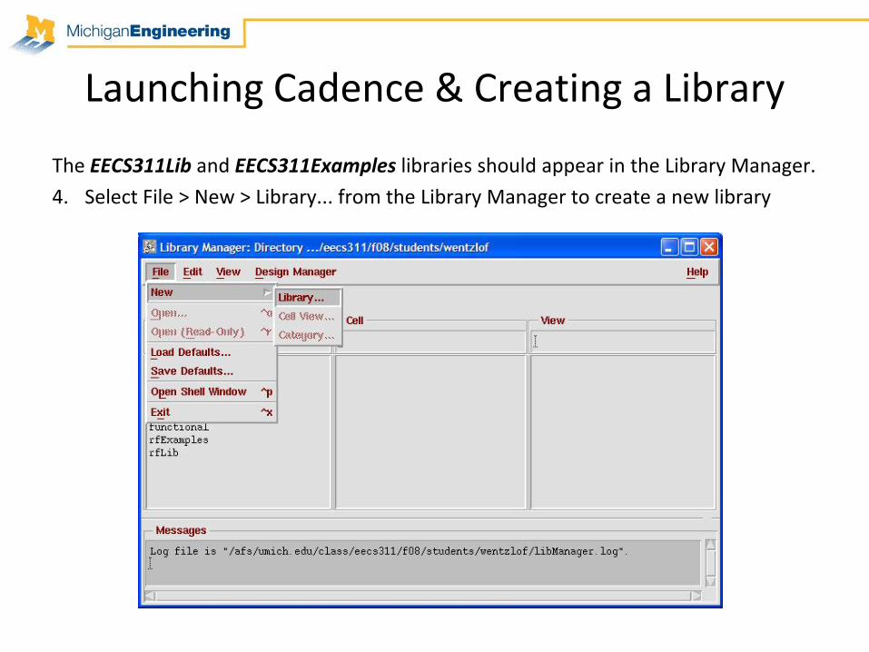
The EECS311Lib and EECS311Examples libraries should appear in the Library Manager.4. Select File > New > Library... from the Library Manager to create a new library

Launching Cadence & Creating a Library

5. Enter tutorial for the Library Name and click OK

6. Select “Don't need a techfile” and click OK

7. The library tutorial should now appear in the Library Manager.

Creating a New Schematic

8. Click on the tutorial library in the Library Manager to select it, then go toFile > New > Cell View...

Creating a New Schematic

9. Type amplifier for the Cell Name, and choose Composer-Schematic for the Tool. The View Name will default to schematic, then click OK.

10. The new schematic will open. To add a part to the schematic, go toAdd > Instance... or by hit the ‘i’ key.

Adding Components

11. To find a part, click Browse from the Add Instance dialog box

12. The Library Browser will pop up. Select EECS311Lib > lab1_opamp > symbol, then click Close.

13. Place the lab1_opamp on the schematic14. Exit the current command by pressing the ‘Esc’ key

Adding Components

Adding Components

15. Add the remaining instances using Add > Instance...Resistors (analogLib > res)Capacitors (analogLib > cap)Pulse generator (analogLib > vpulse)Ground connections (analogLib > gnd)

16. Connect instances as shown in the figure on the next slide.17. Go to Add > Wire Name... to name the Vin and Vout netsAside: To copy an instance, go to Edit > Copy or by hit the ‘c’ key.Aside: To rotate an instance, go to Edit > Rotate or by hit the ‘r’ key.Aside: To edit the properties of an instance, select the component and either go to

Edit > Properties or press the ‘q’ key.Aside: To move an instance, click and drag the component, press the ‘m’ key, or press

shift+‘m’ to break wire connections then move it.Aside: To auto-zoom the schematic, go to Window > Fit or press the ‘f’ key.

Adding Components

Below is the final circuit schematic.

18. Edit the properties of the pulse input to have the following properties:AC magnitude = 1 VDC voltage = 1 VVoltage 1 = 0 VVoltage 2 = Ampl VDelay time = 100u sRise time = 1n sFall time = 1n sPulse width = 2m sPeriod = 4m s

Aside: ‘Voltage 2’ is used for transientsimulations. By giving it a variablename, it can be swept/changed later.

Note: Units are added automatically.

Editing Properties

19. Click the ‘Check and Save’ button in the upper left corner of the schematic window to save the schematic design

20. Go to Tools > Analog Environment to setup simulations

Setting Analog Environment

Setting Design Variables

21. Load variable names from the schematic by selecting Variables > Copy From Cellview

22. Select Variables > Edit ... to edit the variable values or double-click on them in the environment window.

23. Give the Ampl variable a value of 1 (Vpk)

24. Go to Analyses > Choose... or click the “Choose analysis” button on the right-hand side of the Analog Environment Window

25. Select dc as the Analysis type, then select “Save DC Operating Point” and ensure that ‘Enabled’ is selected at the bottom

Setting Analyses

26. Select ac as the Analysis type. Set the Sweep Variable to ‘Frequency’ and sweep over a range from 1 Hz to 10k Hz. Set the Sweep Type to ‘Logarithmic’ with 100 Points Per Decade. Ensure that ‘Enabled’ is selected at the bottom.

Setting Analyses

27. Select tran as the Analysis type. Set the stop time to be 2m s and ensure that ‘Enabled’ is selected at the bottom

Setting Analyses

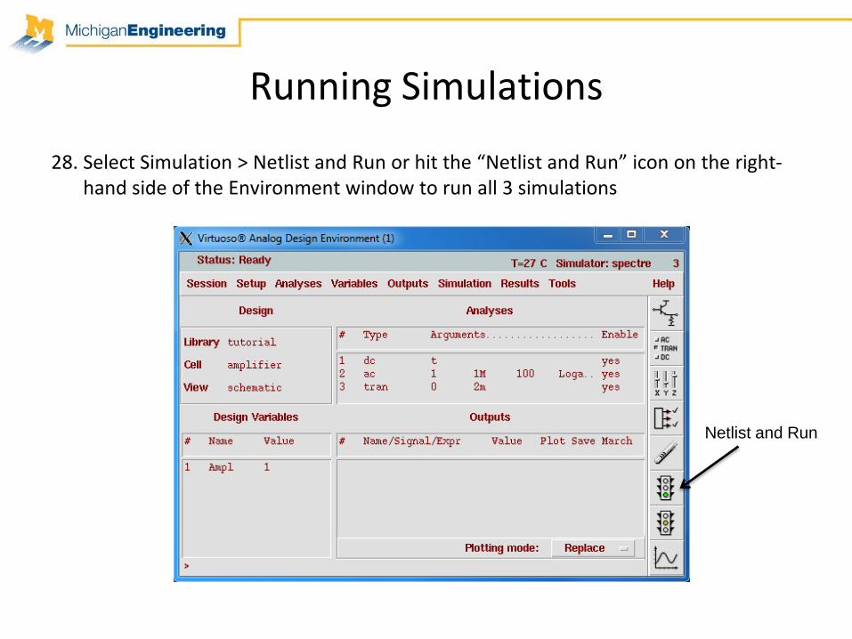
28. Select Simulation > Netlist and Run or hit the “Netlist and Run” icon on the right-hand side of the Environment window to run all 3 simulations

Netlist and Run

Running Simulations

29. To see the DC voltages and currents within the circuit, select Results > Annotate > DC Node Voltages & Results > Annotate > DC Operating Points

The opamp has roughly equal DC voltage at its terminals with no DC current going into either input. The opamp also has a gain of roughly Av = 2 V/V as expected.

View Results

30. To view the small signal response, select Results > Direct Plot > AC Magnitude, then select the Vout wire in the schematic window and press ‘Esc’. (left figure)

31. Select Results > Direct Plot > AC dB20, then select the Vout wire in the schematic window and press ‘Esc’. (right figure)

Viewing Results

Once again, the opamp has a gain of roughly Av = 2 V/V as expected. Because it is non-ideal, the opamp has a finite frequency response.

32. To see the transient response, select Results > Direct Plot > Transient Signal and select both Vin and Vout in the schematic window and press ‘Esc’. (left figure)

33. Go to Zoom > X-Zoom or press ‘x’ to zoom-in the plot. (right figure)

Viewing Results

Once again, the opamp has a gain of roughly Av = 2 V/V after the step response. By zooming-in, we see that the delay is 135μs, which matches the result from the class demo.

S&K Demo: Non-Inverting Amplifier v2

• Build a non-inverting amplifier in Cadence with a gain of 2 V/V• Used the circuit in Fig. 1 in the S&K paper

– Used different resistors

kΩRRnFCC

ΩRkΩRRRAv

1020

50059

1

32

10

1

0

2

3

====

==

+=

.

34. To see the transient response, select Results > Direct Plot > Transient Signal and select both Vin and Vout in the schematic window and press ‘Esc’.

Viewing Results v2

Once again, the opamp has a gain of roughly Av = 2 V/V after the step response, but now we have oscillations like seen in the class demo.

Saving Analog Environment Setup

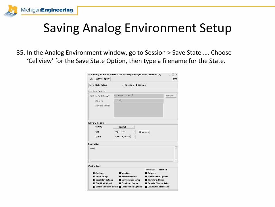
35. In the Analog Environment window, go to Session > Save State …. Choose ‘Cellview’ for the Save State Option, then type a filename for the State.

Saving Results

• There are at least 3 ways to save your plots:1. Hit the ‘Print Screen’ key. In Linux, a window should pop-up that allows you

to save the entire screen.2. In the plot window, go to File > Save as Image…, hit the ‘Browse…’ button,

define the file name and path, click ‘Ok’, and click ‘Ok’ again. This will save the plot as an image.

3. In the plot window, select each trace, then go to Tools > Table…, select ‘Value’, and click ‘Ok’. You should see a speadsheet window open with data. To save the data points, go to File > Save as CSV…, define the file name and path, and click ‘Save’. This will save the data, so that you can generate a clean plot in Matlab.

Better

Best

Good

Using the Linux Terminal

• For those new to Linux, there are many commands to learn within the terminal, which can make your life easier. Below are just a few.>> cd % change directory

>> <any command> --help % brings up help info on <any command>

>> <any command> ~/... % ~ starts a path from your home directory

>> <any command> ./... % . starts a path from your current directory

>> <any command> & % & launches a process in the background

>> ls -a % list all files & folders in a directory

>> ps –u <uniqname> % lists yours processes & process IDs

>> kill <process ID> % kills a process (like Cadence if it freezes)

>> ln -s % create a symbolic link

>> cp % copy

>> mkdir % make directory

>> rm % remove files

>> rmdir % remove directory

>> mv % move or rename files or directory

>> gedit <filename> & % opens a very Windows-like text editor

>> ps2pdf % converts a postscript file to a pdf

• You can search the web and find more commands pretty easily– ss64.com/bash/ has a pretty good list