university of tromsØ cruise report - kielprintseprints.uni-kiel.de/24445/1/eco2 cruise report uit...
TRANSCRIPT

1 NO-9037 Tromsø • [email protected] • http://uit.no • Switchboard: (+47) 77 64 40 00 • Fax: (+47) 77 64 49 00 Department of Geology • Phone 77 64 44 09 • Fax 77 64 56 00
Date: July 31, 2013
UNIVERSITY OF TROMSØ cruise report
Tromsø – Longyearbyen 08-07-13 to 21-07-13
R/V Helmer Hanssen
Cruise No. 2013007
PART I
Sub-seabed CO2 Storage: Impact on Marine Ecosystems (ECO2)
(A 7th Framework Programme EU project)
Institutt for Geologi, Dramsveien 201 Universitetet i Tromsø
Stefan Bünz (chief scientist)
2
Table of Contents
PARTICIPANT LIST ................................................................................................................ 3
INTRODUCTION AND OBJECTIVES ................................................................................... 4
METHODS ................................................................................................................................. 6
Seismic methods ..................................................................................................................... 6
The P-Cable 3D seismic system ............................................................................................. 6
CTD and water sampling ........................................................................................................ 8
Sediment sampling ................................................................................................................. 9
PRELIMINARY RESULTS .................................................................................................... 10
Swath bathymetry onboard processing ................................................................................ 10
CTD casts and water sampling ............................................................................................. 11
P-Cable 3D seismic onboard QC and processing ................................................................. 13
NARRATIVE OF THE CRUISE ............................................................................................. 18
ACKNOWLEDGEMENT ....................................................................................................... 20
APPENDIX .............................................................................................................................. 21
CTD stations ......................................................................................................................... 21
Multicorer Stations ............................................................................................................... 22
3D seismic line log (Lyngen) ........................................................................................... 23
3D seismic line log (Snøhvit) ........................................................................................... 27

3
PARTICIPANT LIST
Stefan Bünz (chief scientist)
University of Tromsø, Norway
Alexandros Tasianas
University of Tromsø, Norway
Sunil Vadakkepuliyambatta
University of Tromsø, Norway
Anoop Nair
University of Tromsø, Norway
Steinar Iversen University of Tromsø, Norway
Andreia Plaza-Faverola University of Tromsø, Norway
Sandra Hurter
University of Tromsø, Norway
Leif Tokle
University of Tromsø, Norway
Espen Valberg University of Tromsø, Norway
Ola Eriksen
P-Cable AS, Oslo, Norway
Jens Greinert
Geomar, Germany
Manuel Bensi
OGS, Italy
Martina Kralj
OGS, Italy
Evgenia Martuganova
MSU, Moscow
Maria Ambrosimova
MSU, Moscow

4
INTRODUCTION AND OBJECTIVES
The ECO2 project sets out to assess the risks associated with the storage of CO2 below the
seabed. Carbon Capture and Storage (CCS) is regarded as a key technology for the reduction
of CO2 emissions from power plants and other sources at the European and international
level. The EU will hence support a selected portfolio of demonstration projects to promote, at
industrial scale, the implementation of CCS in Europe. Several of these projects aim to store
CO2 below the seabed. However, little is known about the short-term and long-term impacts
of CO2 storage on marine ecosystems even though CO2 has been stored sub-seabed in the
North Sea (Sleipner) for over 13 years and for 5 year in the Barents Sea (Snøhvit). Against
this background, the proposed ECO2 project will assess the likelihood of leakage and impact
of leakage on marine ecosystems. In order to do so ECO2 will study a sub-seabed storage site
in operation since 1996 (Sleipner, 90 m water depth), a recently opened site (Snøhvit, 2008,
330 m water depth), and a potential storage site located in the Polish sector of the Baltic Sea
(B3 field site, 80 m water depth) covering the major geological settings to be used for the
storage of CO2. Novel monitoring techniques will be applied to detect and quantify the fluxes
of formation fluids, natural gas, and CO2 from storage sites and to develop appropriate and
effective monitoring strategies. Field work at storage sites will be supported by modelling and
laboratory experiments and complemented by process and monitoring studies at natural CO2
seeps that serve as analogues for potential CO2 leaks at storage sites.
As part of the ECO2 project, the University of Tromsø conducted a cruise in 2011 to the
Snøhvit area in the SW Barents Sea (Figure 1). A high-resolution P-Cable 3D seismic volume
was acquired. This volume constitutes baseline data for monitoring studies. This year we
intend to acquire a second 3D volume (monitor data) from the Snøhvit area. Additional, we
will repeat some of the lines twice and in reversed direction in order to study the repeatability
of the P-Cable acquisition for monitoring purposes. The primary objective of the hydrological
and biogeochemical sampling in the Snohvit area is to study any possible effects of a Carbon
Capture and Storage (CCS) site on the water column and on the bottom sediment.
The Snøhvit reservoir and storage site study area is located in the Hammerfest basin in the
SW Barents Sea approximately 100 nm north off the coast of Norway (Figure 1). The
working areas are in approx. 300 – 400 m water depths. The Snøhvit hydrocarbon field has
been operated by Statoil since 2008. The reservoir lies in Jurassic sandstones at about 2 km
depth. Beneath the reservoir formation, CO2 is stored in Triassic sediments of the Tubaen
formation and later in the bottom part of the Jurassic Stø formation. At Snøhvit, the analysis
of conventional 3D seismic data resulted in the definition of stratigraphic boundaries of the
overburden structure and the identification of faults, gas chimneys and shallow gas
accumulations including the potential occurrence of a gas-hydrate related bottom-simulating
reflection (Figure 1). Faults both at the Jurassic and Tertiary levels have been interpreted.
5
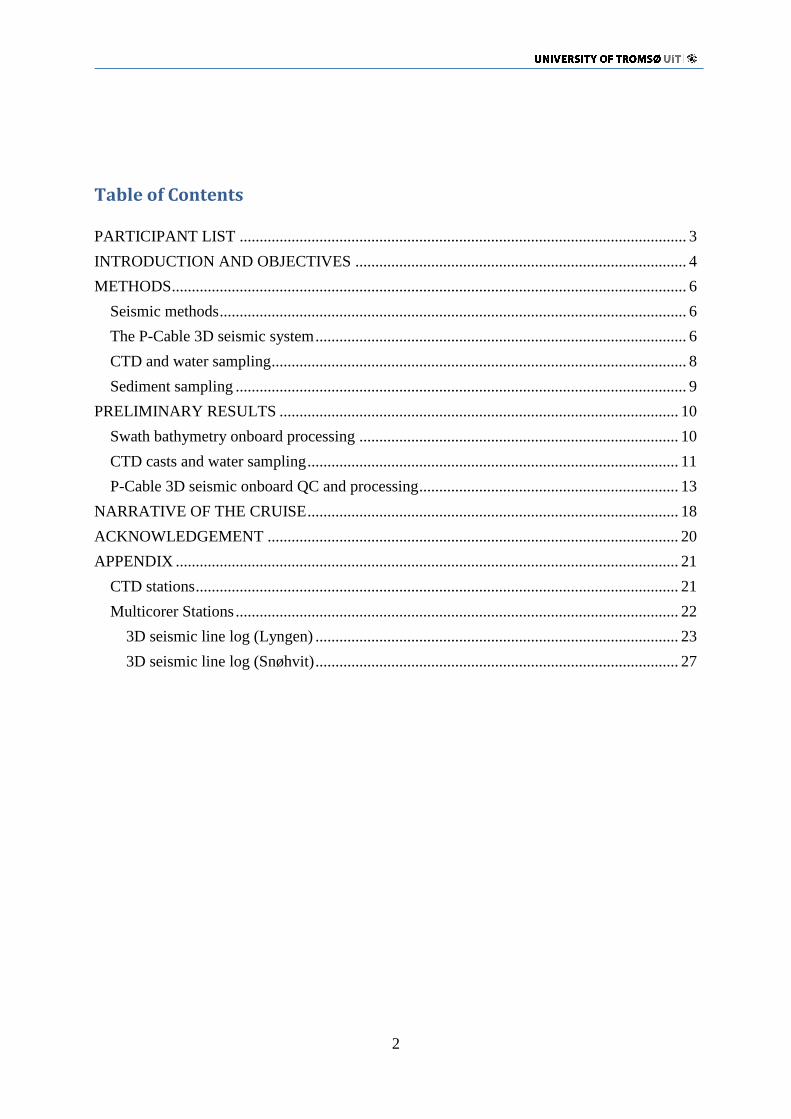
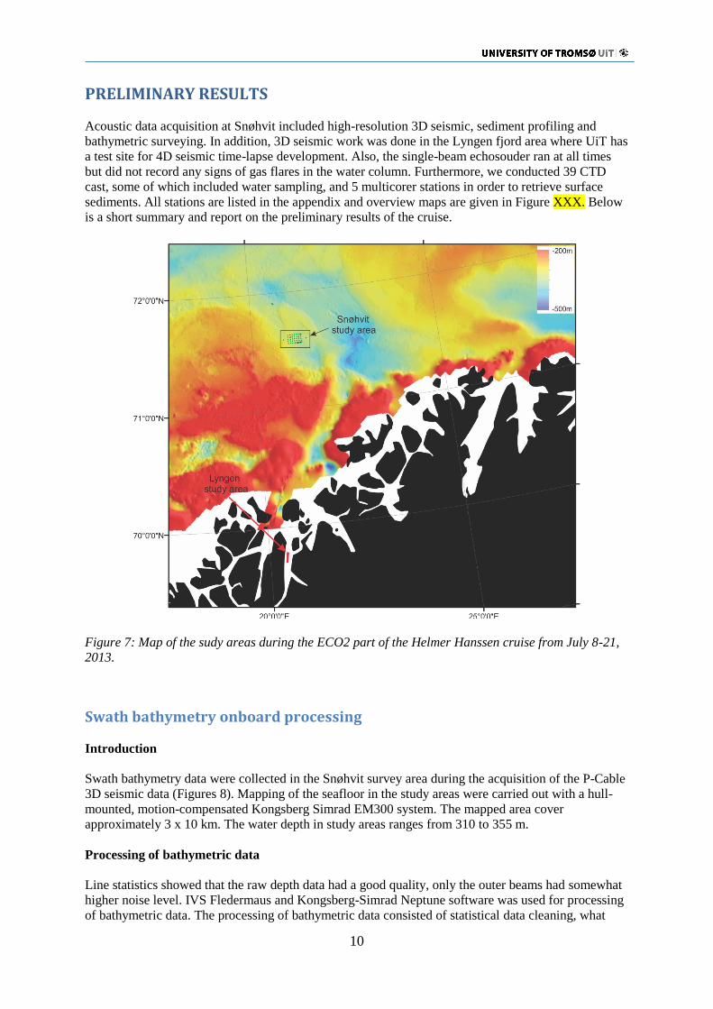
Figure 1: (top) Overview and location of the study area in the SW Barents Sea. (bottom) Perspective
view of the Snøhvit study area based on conventional 3D seismic data. The Main reservoir is in the
Jurassic Stø formation, whereas the CO2 is stored beneath in the Triassic Tubaen formation. The
shallow subsurface shows many amplitude anomalies that can be related to the presence of shallow
gas and gas hydrates.

6
METHODS
Seismic methods
The ECO2 part of the R/V Helmer Hanssen cruise is aimed to acquire P-Cable high-resolution
3D seismic data over pockmark fields, gas chimneys, shallow gas accumulations, and
potential gas hydrate locations at the Snøhvit CO2 storage site. We plan to repeat the whole or
parts of the first baseline P-Cable 3d seismic cube shot over the pockmark field in 2011.
The high-resolution P-Cable 3Dseismic system was used together with a Granzow high-
pressure (210bar) compressor and one mini-GI gun (15/15 in3). Onboard seismic processing
and QC of P-Cable seismic data provided preliminary 3D cubes for quality assessment and
geofluid interpretations.
During this cruise we used SIMRAD EM300 high-resolution multibeam seabed mapping see
report C), P-Cable high-resolution seismic, SIMRAD EK 60 38 and 18 kHz echolot, and the
Edgetech Discover penetration echolot. CTD stations are carried out to extract information
about different (T, S) properties of water masses to calculate the speed of sound for
calibrating the EM300.
The P-Cable 3D seismic system
The P-Cable 3D high-resolution seismic system consists of a seismic cable towed
perpendicular (cross cable) to the vessel's steaming direction (Figure 2). An array of multi-
channel streamers is used to acquire many seismic lines simultaneously, thus covering a large
area with close in-line spacing in a cost efficient way. The cross cable consists of two 50-m
long and one 75-m long section with a total of 14 streamers attached to it. Including lead-in
cables, the cross cable has a total length of 233 m between paravanes (doors) (Figure 2). The
cross-cable is spread by two paravanes that due to their deflectors attempt to move away from
the ship. The paravanes itself are towed using R/V Helmer Hanssen’s large trawl winches.
The spacing between the streamers is 12.5 m but due to curvature of the cross-cable, the
effective spacing between the streamers may be shortened in cross line direction to about 6-12
m. Each digital streamer is 25 meters long and consists of an A/D-module and 8 channels.
New Geometrics solid state streamers are used that are much less affected by sea swell and
hence provide data with significantly less noise. The A/D-module converts the analogical
signal from the channels to digital signals. The group spacing of channels along the streamer
is of 3.125 m.
A 300-m long signal cable is run off the P-Cable winch and connects to the starboard
termination of the cross cable. It contains wiring for power and data transmission. The data is
transferred via Ethernet protocol. Ethernet-to-Coax switches at the ends of the signal cable
allow data transmission over long distances. The digital data is recorded using Geometrics
GeoEel software.

7
Figure 2: Schematic sketch (top) and technical drawing (bottom) of the P-Cable high-resolution 3D
seismic system.

8
Figure 3: Images of the P-Cable system during deployment and recovery. Top left: the cross cable is
being deployed, streamer sections are connected during deployment; top right: The cross cable is
recovered and spooled back on the winch while streamers as disconnected from the cross cable. The
small winch next to the cross cable holds the signal cable; bottom left: inspection of cross cable
junction boxes during deployment and recovery; bottom right: signal cable (red-blue feathered), cross
cable (helical cable in center) and solid state streamer (green) are deployed simultaneously.
CTD and water sampling
Conductivity-Temperature-Depth (CTD) is the oceanographer’s standard tool for determining oceanic
water masses. SeaBird’s (SBE) 911plus CTD was used for oceanographic measurements. The
following parameters were measured: temperature, conductivity and pressure (converted to depth),
speed of sound, fluorescence and turbidity. The temperature sensor is located at the base of the
Rosette, thereby being the first sensor to measure the undisturbed water mass on the downcast.
Furthermore, water is pumped through a conductivity tube, in which seawater conductivity is
measured. Continuous pump operation is essential to prevent boundary layers forming on the tube’s
edges, and should data sets indicate fault malfunctions the data sets are flagged or deleted. CTD data
was acquired and processed using SBE’s in-house “SBE Data Processing”.
A rosette with 12 Niskin bottles (10L) was used for water samples collection. Dissolved oxygen
concentration (Titrator, Winkler method) and pH (pHmeter) measurements were done directly onboard
after each CTD cast (Fig. 1). Furthermore, the following analyses will be performed on the water
samples (approximately 60) at the OGS laboratory: pH (spectrophotometric), CO2, CH4, Dissolved
Inorganic Carbon (DIC), Dissolved Organic Carbon (DOC), Nutrients, Dissolved Organic Nitrogen
and Phosphate. Additionally, 12 bottles of salinity samples were collected in order to check the
stability of the conductivity sensor during the whole cruise.
9
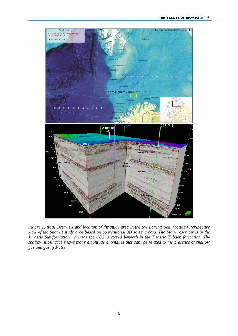
Figure 4: CTD SBE911plus (on the left) used for hydrological and biogeochemical water samples and
instruments for dissolved oxygen concentration and pH analyses on board (on the right).
Sediment sampling
Sediment sampling was done using a multicorer system with 6 liners (Figure 4). A total of five
multicorer stations were successfully completed. Two of these five stations are within larger
pockmarks in the Snøhvit area, and one other station lies approximately 20 nm to the northwest and
constitutes a reference station. At least 4 of the 6 liners were filled with sediments at all stations and
retrieval was up to about 40 cm. Sediments were extruded from the liner and sub-sampled (Figure 5).
Figure 5: Multicorer after sediment collection.
Figure 6: Slicing of the sub-bottom sediment
layers.
10
PRELIMINARY RESULTS
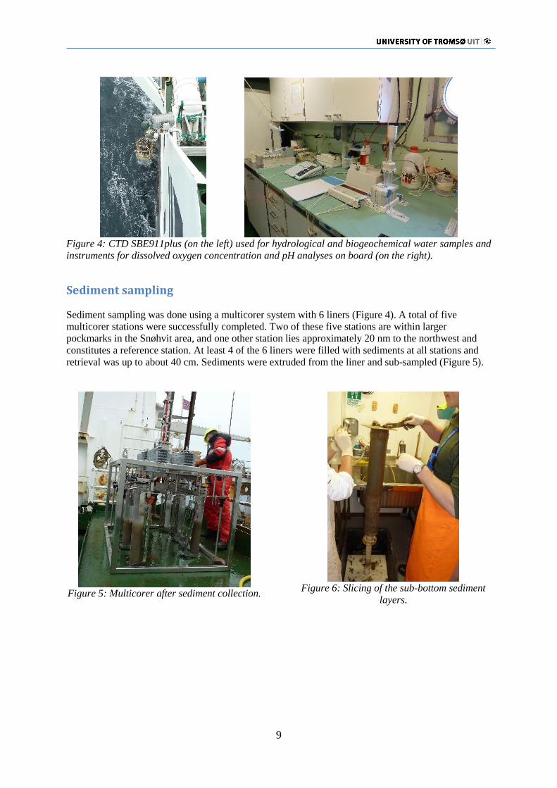
Acoustic data acquisition at Snøhvit included high-resolution 3D seismic, sediment profiling and
bathymetric surveying. In addition, 3D seismic work was done in the Lyngen fjord area where UiT has
a test site for 4D seismic time-lapse development. Also, the single-beam echosouder ran at all times
but did not record any signs of gas flares in the water column. Furthermore, we conducted 39 CTD
cast, some of which included water sampling, and 5 multicorer stations in order to retrieve surface
sediments. All stations are listed in the appendix and overview maps are given in Figure XXX. Below
is a short summary and report on the preliminary results of the cruise.
Figure 7: Map of the sudy areas during the ECO2 part of the Helmer Hanssen cruise from July 8-21,
2013.
Swath bathymetry onboard processing
Introduction
Swath bathymetry data were collected in the Snøhvit survey area during the acquisition of the P-Cable
3D seismic data (Figures 8). Mapping of the seafloor in the study areas were carried out with a hull-
mounted, motion-compensated Kongsberg Simrad EM300 system. The mapped area cover
approximately 3 x 10 km. The water depth in study areas ranges from 310 to 355 m.
Processing of bathymetric data
Line statistics showed that the raw depth data had a good quality, only the outer beams had somewhat
higher noise level. IVS Fledermaus and Kongsberg-Simrad Neptune software was used for processing
of bathymetric data. The processing of bathymetric data consisted of statistical data cleaning, what

11
was done block by block in BinStat. This function ensures an adaptive way of filtering and taking
changes in the seabed terrain into account. In addition, raw data were also cleaned manually and
visually with interactive graphical editors to improve the accuracy on the depth data. After processing,
the bathymetry data set was gridded in the interactive visualization system Fledermaus. The good
density of measurement point allowed a grid cell size of 4 m x 4 m.
Morphological features interpretation
More or less linear and sinuous features are observed almost everywhere on the seafloor in both areas
(Figures 8). They are furrows with a small rise on both sides. The furrows are several km long and up
400 m wide, but most of furrows are 1-2 km long and up to 100 m wide. They have a U-shape in a
vertical profile and their shape is slightly smooth. Their depths range between 3 and 5 m. The
dominant furrow orientation is ENE - WSW but the direction varies greatly. In some cases, the
furrows cross-cut each other and at the end point, the furrows create a headwall. Those features were
interpreted to be iceberg ploughmarks. Iceberg ploughmarks are formed when the keel of an iceberg is
exceeding the water depth and erodes soft sediments. Ploughmarks indicate that the region has been
influenced by glacial processes and are evidence of iceberg activity.
The seafloor in area 1 shows hundreds of small and a few large depressions (Figure 8). These
depressions are typical expressions of fluid escape through the seafloor and are called pockmarks. The
mapping confirms observations from 2011. Two different pockmarks classes occur in the area:
hundreds of small pockmarks with diameters of up to 20 m and depth of up to 1 m, and very few large
pockmarks with diameters of up 700 m and depth of up to 10 m. Hydro-acoustic surveying did not
detect any indications for gas leakage from the seafloor.
Figure 8: Bathymetric map of the study area at Snøhvit acquired simultaneously with the P-Cable 3D
seismic data. A dense line spacing and slow ship’s speed allows a high-resolution mapping (4m bins)
of the seafloor.
CTD casts and water sampling
A synoptic collection of CTD profiles, water and sediment samples were performed in a
restricted area of approximately 12x8km, which coincides with the seismic working area
planned by the UiT (Figure 9). In particular, 37 CTD profiles (2 km distance from each other)
were collected in the study area, 2 additional CTD profiles were acquired 5km east and west
of the main area and 1 CTD station was located at about 40-50 km north of the Snohvit area
and used as a reference station. At 14 stations water samples were collected only in the
bottom layer (at 2 depths: bottom and ~280m, plus two additional quotes for dissolved oxygen
samples), while at 5 stations water samples were collected throughout the whole water
column (6 depths were chosen, based on the vertical variability: bottom, ~280m, ~200m,
~110m, ~70m, ~30m). The selection of the 5 stations cited above was located at the following
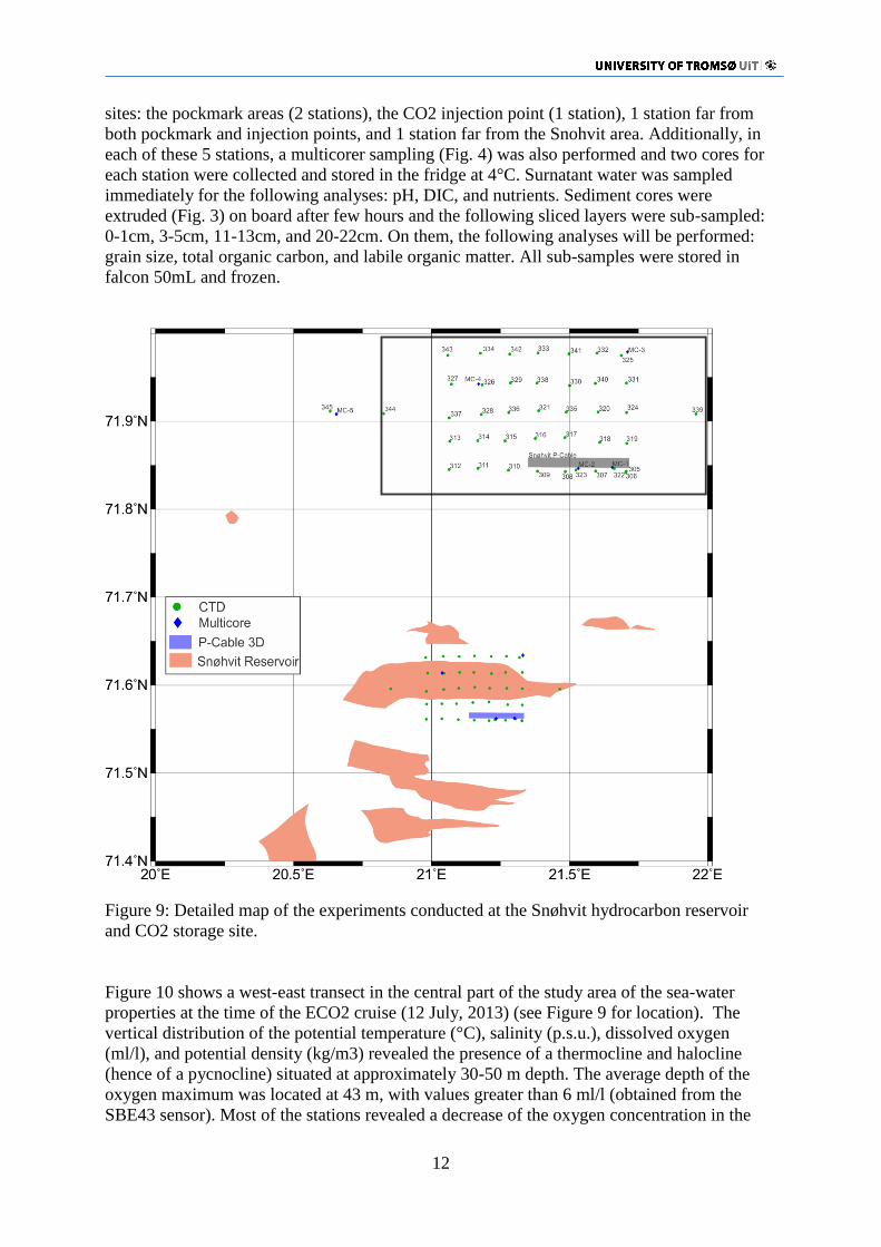
12
sites: the pockmark areas (2 stations), the CO2 injection point (1 station), 1 station far from
both pockmark and injection points, and 1 station far from the Snohvit area. Additionally, in
each of these 5 stations, a multicorer sampling (Fig. 4) was also performed and two cores for
each station were collected and stored in the fridge at 4°C. Surnatant water was sampled
immediately for the following analyses: pH, DIC, and nutrients. Sediment cores were
extruded (Fig. 3) on board after few hours and the following sliced layers were sub-sampled:
0-1cm, 3-5cm, 11-13cm, and 20-22cm. On them, the following analyses will be performed:
grain size, total organic carbon, and labile organic matter. All sub-samples were stored in
falcon 50mL and frozen.
Figure 9: Detailed map of the experiments conducted at the Snøhvit hydrocarbon reservoir
and CO2 storage site.
Figure 10 shows a west-east transect in the central part of the study area of the sea-water
properties at the time of the ECO2 cruise (12 July, 2013) (see Figure 9 for location). The
vertical distribution of the potential temperature (°C), salinity (p.s.u.), dissolved oxygen
(ml/l), and potential density (kg/m3) revealed the presence of a thermocline and halocline
(hence of a pycnocline) situated at approximately 30-50 m depth. The average depth of the
oxygen maximum was located at 43 m, with values greater than 6 ml/l (obtained from the
SBE43 sensor). Most of the stations revealed a decrease of the oxygen concentration in the
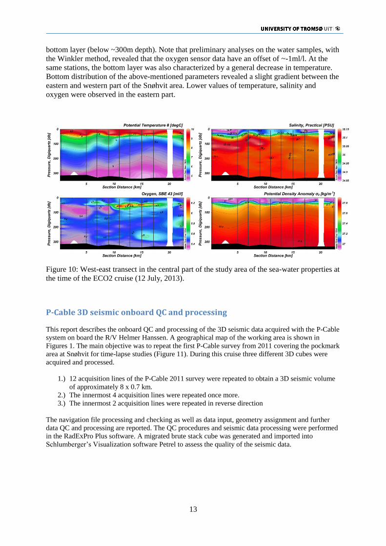
13
bottom layer (below ~300m depth). Note that preliminary analyses on the water samples, with
the Winkler method, revealed that the oxygen sensor data have an offset of ~-1ml/l. At the
same stations, the bottom layer was also characterized by a general decrease in temperature.
Bottom distribution of the above-mentioned parameters revealed a slight gradient between the
eastern and western part of the Snøhvit area. Lower values of temperature, salinity and
oxygen were observed in the eastern part.
Figure 10: West-east transect in the central part of the study area of the sea-water properties at
the time of the ECO2 cruise (12 July, 2013).
P-Cable 3D seismic onboard QC and processing
This report describes the onboard QC and processing of the 3D seismic data acquired with the P-Cable
system on board the R/V Helmer Hanssen. A geographical map of the working area is shown in
Figures 1. The main objective was to repeat the first P-Cable survey from 2011 covering the pockmark
area at Snøhvit for time-lapse studies (Figure 11). During this cruise three different 3D cubes were
acquired and processed.
1.) 12 acquisition lines of the P-Cable 2011 survey were repeated to obtain a 3D seismic volume
of approximately 8 x 0.7 km.
2.) The innermost 4 acquisition lines were repeated once more.
3.) The innermost 2 acquisition lines were repeated in reverse direction
The navigation file processing and checking as well as data input, geometry assignment and further
data QC and processing are reported. The QC procedures and seismic data processing were performed
in the RadExPro Plus software. A migrated brute stack cube was generated and imported into
Schlumberger’s Visualization software Petrel to assess the quality of the seismic data.

14
Figure 11: Seafloor map (Courtesy of Statoil) of parts of the Snøhvit area showing several hundreds of
small pockmarks. The blue box indicates the location of the P-Cable 3D seismic survey acquired in
2011. The red box indicates the extent of the partial repetition of the 2011 survey. The yellow box
indicates the area of a second repetition of the innermost 4 acquisition lines. In addition, the two
innermost lines have been repeated in reversed direction.
Data Input
Seismic data were loaded from seg-d files and saved as RadExPro datasets within the RadExPro
project database. In both areas, the lines were loaded separately directly after acquisition to be sure to
correct for geometry input . Afterwards, the lines were loaded by blocks to one dataset.
Geometry Input
The geometry characteristics of the P-Cable system in this survey are described below. The P-Cable
system was configured with 14 streamers that have 12.5 meters distance between streamers. Distance
from Paravanes to the first and last streamers was 24.25 m and 24 m. Geometry was loaded with the
P-cable geometry modulefrom RadExPro using the parameters listed before. Navigation files were
prepared with Matlab. Alpha trimmed averaging of raw navigation was involved in geometry input
routine prior to geometry assignment. The geometry for every part was assigned in a similar way.
There were no problems with navigation assignments and the geometry was used for all shots.
Geometry Check
After geometry input the assigned geometry was checked for consistence. Observed direct wave
arrival time was compared with one calculated from the assigned geometry. To calculate this time,
velocity in the water column was derived from CTD stations to be 1.477 km/s in the SnøeHvit area
and 1.464 km/s in the Vestnesa area. Quality control was performed by visualizing every 10 common
shot point gather. Figure 12 shows an example of such a QC plot. On some shots the difference
between calculated direct wave arrival time and observed one was about 3 ms, but on most shots the
calculated time fitted the observed one well. Such difference can be caused by strong currents in the
area and bad ship positioning.

15
Figure 12: shot gathers for line 5 in Snøhvit survey. Blue is predicted picks of first arrivals
pick1=offset/Vwater; green is automatic shift to closest through in a 15 ms window; red is bulk shift of
pick2 by 1.5 ms to fit the zero crossing pick-trough corresponding to the first arrival times..
Binning and coverage
The CDP coverage is shown on Figures 13. As one can see there are some small gaps in final coverage
of both areas, bur particularly in area 2. A good coverage depends on ship navigation and line
tracking. In few instances the ship was off the planned line by up to 20 m, which results in the gaps.
However, these gaps mostly are only one bin size wide and thus, can be easily infilled during
processing.
Figure 13: CDP coverage with 8 of 12 lines from the SnøHvit survey.
Partial cubes, brute stacks and QC coverage
As data acquisition continued, partial brute stacks were calculated over the available subset of seismic
lines to assess gaps in the coverage and seismic data quality. Coverage control is very important
during data acquisition. Coverage of the data was controlled using QC plots generated in the
RadExPro. Locations of CDP points were displayed in the 3D CDP Binning tool. At the end of each
area coverage plots were made for all lines, and a brute stack cube for each area was generated. The
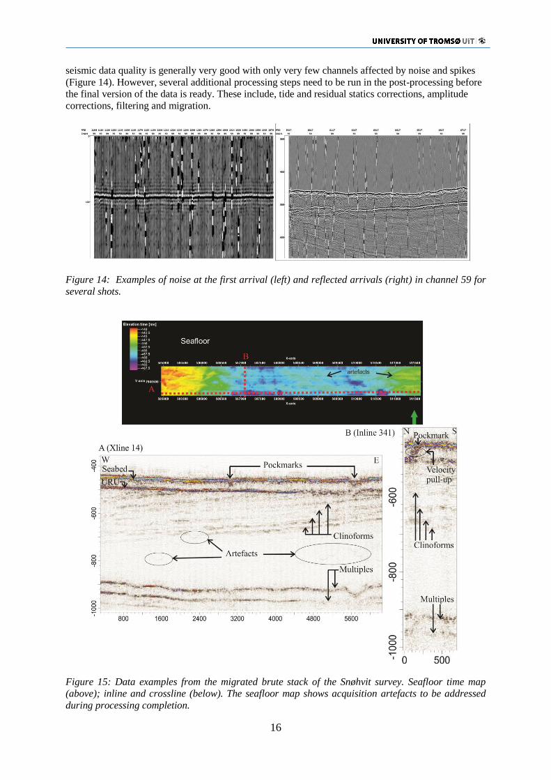
16
seismic data quality is generally very good with only very few channels affected by noise and spikes
(Figure 14). However, several additional processing steps need to be run in the post-processing before
the final version of the data is ready. These include, tide and residual statics corrections, amplitude
corrections, filtering and migration.
Figure 14: Examples of noise at the first arrival (left) and reflected arrivals (right) in channel 59 for
several shots.
Figure 15: Data examples from the migrated brute stack of the Snøhvit survey. Seafloor time map
(above); inline and crossline (below). The seafloor map shows acquisition artefacts to be addressed
during processing completion.

17
The migrated brute stack data was imported into Schlumberger’s Visualization software Petrel for data
quality assessment. The seismic data is of very good quality and shows a strong reflection about 50 ms
below the seafloor associated with the Upper Regional Unconformity (URU) (Figure 15). Several
inclined reflection are related to the previously identified clinoform system below URU. The seafloor
and the URU reflection were interpreted (Figure 15 & 16). Both surfaces show similar features
compared to the 2011 baseline data. However, there are also several artefacts in statics and amplitudes
that are related to the acquisition. These will be addressed during further processing subsequent to the
cruise.
Figure 16: Map showing the Upper Regional Unconformity (URU) (Figure 15) interpreted from the
brute stack data.
18
NARRATIVE OF THE CRUISE
Times in this report are given in local time (local time -2 hrs = UTC), 3D seismic data are
logged in UTC time and ship logs are given in UTC time. Weather conditions at the start of
the cruise were bad and did not allow us to leave the shelter of the fjords for two days.
Afterwards, weather and sea state improved and were calm to slightly rough (Bft 3-5) with
mostly grey skies. Air temperatures were between 5 oC and 12 oC. We started to prepare the
cruise in Tromsø on July 8 with loading and assembling all seismic equipment.
Monday, 08.07.
The scientific crew arrived during the afternoon hours. We started to load all equipment
onboard the ship and began assembling the seismic equipment. Cables were spooled onto the
winches. Electronics and computers for seismic data acquisition is set up in the laboratory.
Loading and assembling lasted until into the evening hours. The last participants from
Moscow State University arrived late at midnight. Missed baggage on the flight forced us to
delay our departure. However, gale winds and high waves (4-5 m) in the SW Barents Sea
wouldn’t have us allowed to leave the shelter of the coastline anyhow.
Tuesday, 09.07.
14:00 The missed baggage arrived and we depart from Tromsø heading north to the Lyngen
Fjord area. Weather hasn’t calmed down and we can’t leave to the open sea. We will test and
eploy the P-Cable system in the Fjord in the University of Tromsø 4D seismic test area. Here,
we will acquire a few more lines for 4D seismic analysis to further develop the P-Cable
system into a monitoring tool.
20:00: We acquire a CTD cast in 314 m water depth and hydroacoustic systems onboard are
calibrated with sound velocity in water.
20:30: Start of the deployment of the P-Cable system.
22:30: Intermediate test showed no sign of problems. However, after the whole system is in
the water, we discover high leakage causing communication problems.
23:00: The recovery of the end of the cross cable showed water leakage into a terminating
connector causing an electrical shortcut and damaging of the last Ethernet junction of the
cross cable. We replace the last cross cable section.
23:30: However, problems persist without clear indication of its cause.
Wednesday, 10.07.
01:30 Several test do not provide any further indication of the problem and we recover the
whole system to systematically test individual parts.
03:00: There are indications that there are unwanted signals on the trigger line that cause A/D
digitizers to reset. These problems could be related to the signal cable. However, as it is late at
night and everybody has worked hard, we need to call of work for the night.
08:30: After breakfast, troubleshooting on the P-Cable system continues. Errors seem to be
random and related to problems with detecting the A/D cans.
13:30 We have almost changed all parts of the system but still experience problems. When all
sections have been detected it appears running fine. But then problems re-appear on the next
setup.
17:00 A/D digitizers are now being programmed individually by hardcoding the IP address.
21:00 Several more test showed a unusual behaviour of the digitizers. These would be off on
SPSU power up, but would come alive on a simple Ethernet ping. Once alive, the system
seem to work fine and we decide to deploy.
23:00 Start of deployment
19
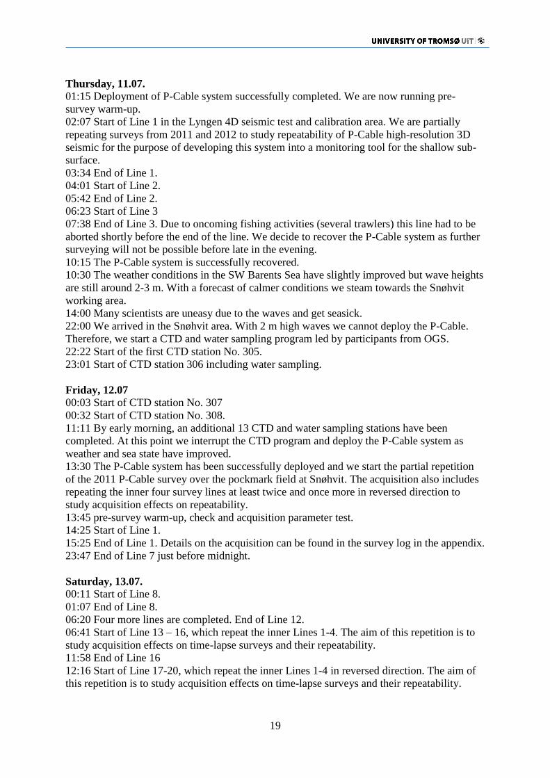
Thursday, 11.07.
01:15 Deployment of P-Cable system successfully completed. We are now running pre-
survey warm-up.
02:07 Start of Line 1 in the Lyngen 4D seismic test and calibration area. We are partially
repeating surveys from 2011 and 2012 to study repeatability of P-Cable high-resolution 3D
seismic for the purpose of developing this system into a monitoring tool for the shallow sub-
surface.
03:34 End of Line 1.
04:01 Start of Line 2.
05:42 End of Line 2.
06:23 Start of Line 3
07:38 End of Line 3. Due to oncoming fishing activities (several trawlers) this line had to be
aborted shortly before the end of the line. We decide to recover the P-Cable system as further
surveying will not be possible before late in the evening.
10:15 The P-Cable system is successfully recovered.
10:30 The weather conditions in the SW Barents Sea have slightly improved but wave heights
are still around 2-3 m. With a forecast of calmer conditions we steam towards the Snøhvit
working area.
14:00 Many scientists are uneasy due to the waves and get seasick.
22:00 We arrived in the Snøhvit area. With 2 m high waves we cannot deploy the P-Cable.
Therefore, we start a CTD and water sampling program led by participants from OGS.
22:22 Start of the first CTD station No. 305.
23:01 Start of CTD station 306 including water sampling.
Friday, 12.07
00:03 Start of CTD station No. 307
00:32 Start of CTD station No. 308.
11:11 By early morning, an additional 13 CTD and water sampling stations have been
completed. At this point we interrupt the CTD program and deploy the P-Cable system as
weather and sea state have improved.
13:30 The P-Cable system has been successfully deployed and we start the partial repetition
of the 2011 P-Cable survey over the pockmark field at Snøhvit. The acquisition also includes
repeating the inner four survey lines at least twice and once more in reversed direction to
study acquisition effects on repeatability.
13:45 pre-survey warm-up, check and acquisition parameter test.
14:25 Start of Line 1.
15:25 End of Line 1. Details on the acquisition can be found in the survey log in the appendix.
23:47 End of Line 7 just before midnight.
Saturday, 13.07.
00:11 Start of Line 8.
01:07 End of Line 8.
06:20 Four more lines are completed. End of Line 12.
06:41 Start of Line 13 – 16, which repeat the inner Lines 1-4. The aim of this repetition is to
study acquisition effects on time-lapse surveys and their repeatability.
11:58 End of Line 16
12:16 Start of Line 17-20, which repeat the inner Lines 1-4 in reversed direction. The aim of
this repetition is to study acquisition effects on time-lapse surveys and their repeatability.
20
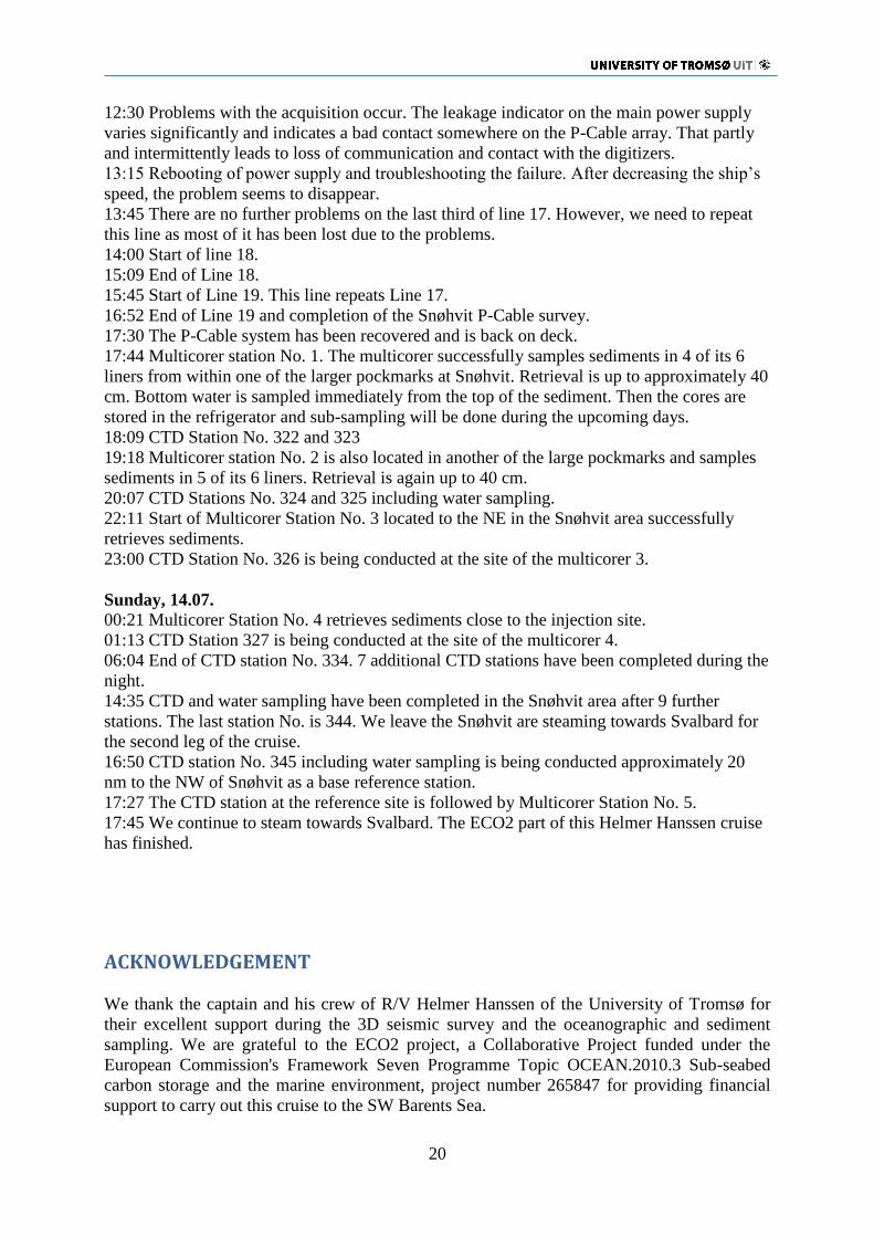
12:30 Problems with the acquisition occur. The leakage indicator on the main power supply
varies significantly and indicates a bad contact somewhere on the P-Cable array. That partly
and intermittently leads to loss of communication and contact with the digitizers.
13:15 Rebooting of power supply and troubleshooting the failure. After decreasing the ship’s
speed, the problem seems to disappear.
13:45 There are no further problems on the last third of line 17. However, we need to repeat
this line as most of it has been lost due to the problems.
14:00 Start of line 18.
15:09 End of Line 18.
15:45 Start of Line 19. This line repeats Line 17.
16:52 End of Line 19 and completion of the Snøhvit P-Cable survey.
17:30 The P-Cable system has been recovered and is back on deck.
17:44 Multicorer station No. 1. The multicorer successfully samples sediments in 4 of its 6
liners from within one of the larger pockmarks at Snøhvit. Retrieval is up to approximately 40
cm. Bottom water is sampled immediately from the top of the sediment. Then the cores are
stored in the refrigerator and sub-sampling will be done during the upcoming days.
18:09 CTD Station No. 322 and 323
19:18 Multicorer station No. 2 is also located in another of the large pockmarks and samples
sediments in 5 of its 6 liners. Retrieval is again up to 40 cm.
20:07 CTD Stations No. 324 and 325 including water sampling.
22:11 Start of Multicorer Station No. 3 located to the NE in the Snøhvit area successfully
retrieves sediments.
23:00 CTD Station No. 326 is being conducted at the site of the multicorer 3.
Sunday, 14.07.
00:21 Multicorer Station No. 4 retrieves sediments close to the injection site.
01:13 CTD Station 327 is being conducted at the site of the multicorer 4.
06:04 End of CTD station No. 334. 7 additional CTD stations have been completed during the
night.
14:35 CTD and water sampling have been completed in the Snøhvit area after 9 further
stations. The last station No. is 344. We leave the Snøhvit are steaming towards Svalbard for
the second leg of the cruise.
16:50 CTD station No. 345 including water sampling is being conducted approximately 20
nm to the NW of Snøhvit as a base reference station.
17:27 The CTD station at the reference site is followed by Multicorer Station No. 5.
17:45 We continue to steam towards Svalbard. The ECO2 part of this Helmer Hanssen cruise
has finished.
ACKNOWLEDGEMENT
We thank the captain and his crew of R/V Helmer Hanssen of the University of Tromsø for
their excellent support during the 3D seismic survey and the oceanographic and sediment
sampling. We are grateful to the ECO2 project, a Collaborative Project funded under the
European Commission's Framework Seven Programme Topic OCEAN.2010.3 Sub-seabed
carbon storage and the marine environment, project number 265847 for providing financial
support to carry out this cruise to the SW Barents Sea.

21
APPENDIX
CTD stations
Date Time(UTC) St. No. Lat. Long. Depth
11.07.2013 20:22:57 305 7133.581860 N 02119.556544 E 327.21
11.07.2013 21:01:58 306 7133.621426 N 02119.610368 E 332.03
11.07.2013 22:03:59 307 7133.631577 N 02116.033720 E 337.42
11.07.2013 22:32:48 308 7133.611086 N 02112.459607 E 340.08
12.07.2013 00:05:23 309 7133.626235 N 02109.186139 E 327.15
12.07.2013 00:41:03 310 7133.667651 N 02105.768816 E 322.71
12.07.2013 01:41:04 311 7133.734598 N 02102.187961 E 318.92
12.07.2013 02:18:43 312 7133.694080 N 02058.818706 E 310.03
12.07.2013 03:17:29 313 7134.735360 N 02058.887822 E 314.04
12.07.2013 03:50:23 314 7134.763516 N 02102.169218 E 315.45
12.07.2013 04:37:34 315 7134.756960 N 02105.375471 E 322.58
12.07.2013 05:14:14 316 7134.844622 N 02108.939294 E 329.18
12.07.2013 06:01:43 317 7134.875524 N 02112.411215 E 339.06
12.07.2013 06:32:42 318 7134.699893 N 02116.506727 E 338.34
12.07.2013 07:58:27 319 7134.662066 N 02119.683416 E 330.61
12.07.2013 08:33:43 320 7135.823275 N 02116.308724 E 335.67
12.07.2013 09:11:38 321 7135.870216 N 02109.330357 E 327.27
13.07.2013 18:09:47 322 7133.725614 N 02118.221940 E 337.82
13.07.2013 18:45:07 323 7133.676468 N 02113.706905 E 338.68
13.07.2013 20:07:45 324 7135.799741 N 02119.679335 E 331.92
13.07.2013 21:00:24 325 7137.914415 N 02119.053535 E 332.62
13.07.2013 23:00:01 326 7136.831686 N 02102.683420 E 316.44
14.07.2013 01:13:57 327 7136.857247 N 02059.080926 E 316.5
14.07.2013 02:10:19 328 7135.732950 N 02102.584043 E 319.24
14.07.2013 02:43:23 329 7136.902534 N 02106.022091 E 322.61
14.07.2013 03:30:59 330 7136.803115 N 02112.966235 E 336.19
14.07.2013 03:53:59 331 7136.897686 N 02119.645935 E 336.26
14.07.2013 04:29:43 332 7138.004160 N 02116.191956 E 334.23
14.07.2013 05:09:45 333 7138.013123 N 02109.259874 E 329.44
14.07.2013 05:46:37 334 7137.998301 N 02102.484715 E 316.56
14.07.2013 06:39:32 335 7135.818581 N 02112.568130 E 338.9
14.07.2013 07:43:35 336 7135.804939 N 02105.804883 E 320.27
14.07.2013 08:40:23 337 7135.604564 N 02058.812564 E 315.19
14.07.2013 09:45:32 338 7136.891853 N 02109.124517 E 328.51
14.07.2013 10:59:02 339 7135.752574 N 02127.827962 E 331.18
14.07.2013 11:41:00 340 7136.884446 N 02115.999658 E 331.02
14.07.2013 12:19:39 341 7137.982958 N 02112.888079 E 328.69
14.07.2013 12:56:33 342 7137.964858 N 02105.936156 E 321.92
14.07.2013 13:44:39 343 7137.921414 N 02058.661841 E 317.39
22
14.07.2013 14:35:09 344 7135.765161 N 02051.082493 E 320.73
14.07.2013 16:50:37 345 7154.708503 N 02037.879327 E 367.47
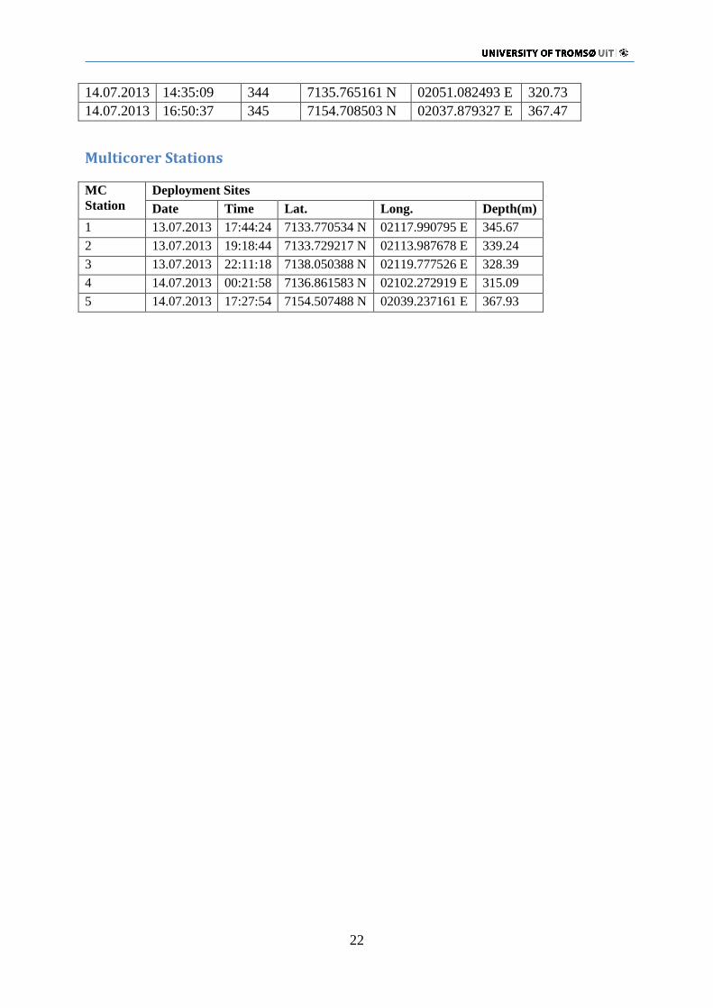
Multicorer Stations
MC
Station
Deployment Sites
Date Time Lat. Long. Depth(m)
1 13.07.2013 17:44:24 7133.770534 N 02117.990795 E 345.67
2 13.07.2013 19:18:44 7133.729217 N 02113.987678 E 339.24
3 13.07.2013 22:11:18 7138.050388 N 02119.777526 E 328.39
4 14.07.2013 00:21:58 7136.861583 N 02102.272919 E 315.09
5 14.07.2013 17:27:54 7154.507488 N 02039.237161 E 367.93
23
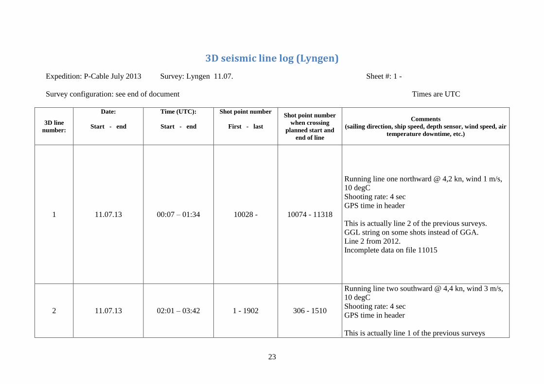
3D seismic line log (Lyngen)
Expedition: P-Cable July 2013 Survey: Lyngen 11.07. Sheet #: 1 -
Survey configuration: see end of document Times are UTC
3D line
number:
Date:
Start - end
Time (UTC):
Start - end
Shot point number
First - last
Shot point number
when crossing
planned start and
end of line
Comments
(sailing direction, ship speed, depth sensor, wind speed, air
temperature downtime, etc.)
1 11.07.13 00:07 – 01:34 10028 - 10074 - 11318
Running line one northward @ 4,2 kn, wind 1 m/s,
10 degC
Shooting rate: 4 sec
GPS time in header
This is actually line 2 of the previous surveys.
GGL string on some shots instead of GGA.
Line 2 from 2012.
Incomplete data on file 11015
2 11.07.13 02:01 – 03:42 1 - 1902 306 - 1510
Running line two southward @ 4,4 kn, wind 3 m/s,
10 degC
Shooting rate: 4 sec
GPS time in header
This is actually line 1 of the previous surveys

24
(2012).
3
11.07.13 04:23 – 05:38 1 - 238 - 1352
Running line three northward @ 4,4 kn, wind 3 m/s,
10 degC
Shooting rate: 4 sec
GPS time in header
This is the second run of line 2 of the previous
surveys (2012).
Aborting line due to fishing activity. Lgsp 1352
25
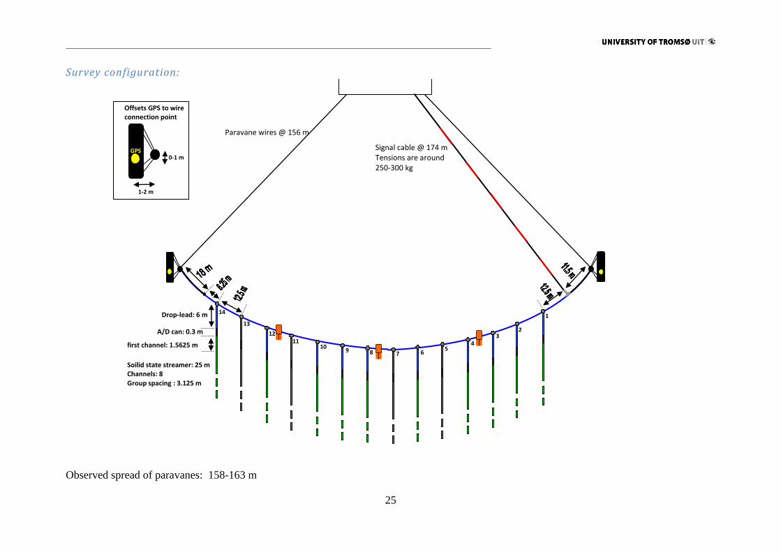
Survey configuration:
Observed spread of paravanes: 158-163 m
Paravane wires @ 156 m
Signal cable @ 174 m Tensions are around 250-300 kg
1
2 3
4 5
6 7 8 9 10
11 12
13
14 Drop-lead: 6 m
A/D can: 0.3 m
Soilid state streamer: 25 m Channels: 8 Group spacing : 3.125 m
Offsets GPS to wire connection point
0-1 m
1-2 m
GPS
first channel: 1.5625 m

26
Observed distance between gun and paravanes: 93 – 103 m, deviations between distances to both paravanes up to 5 m
Gun system: mini-GI (15/15 in3)
Shooting pressure: ~160 bar
Shooting interval: 4 sec
Recording length: 1.5 sec
27
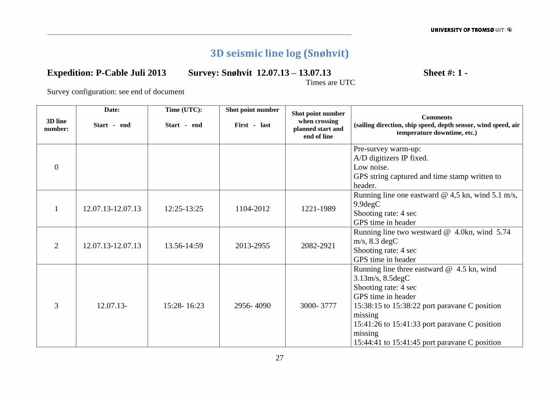
3D seismic line log (Snøhvit)
Expedition: P-Cable Juli 2013 Survey: Snøhvit 12.07.13 – 13.07.13 Sheet #: 1 - Times are UTC
Survey configuration: see end of document
3D line
number:
Date:
Start - end
Time (UTC):
Start - end
Shot point number
First - last
Shot point number
when crossing
planned start and
end of line
Comments
(sailing direction, ship speed, depth sensor, wind speed, air
temperature downtime, etc.)
0
Pre-survey warm-up:
A/D digitizers IP fixed.
Low noise.
GPS string captured and time stamp written to
header.
1 12.07.13-12.07.13 12:25-13:25 1104-2012 1221-1989
Running line one eastward @ 4,5 kn, wind 5.1 m/s,
9.9degC
Shooting rate: 4 sec
GPS time in header
2 12.07.13-12.07.13 13.56-14:59 2013-2955 2082-2921
Running line two westward @ 4.0kn, wind 5.74
m/s, 8.3 degC
Shooting rate: 4 sec
GPS time in header
3 12.07.13- 15:28- 16:23 2956- 4090 3000- 3777
Running line three eastward @ 4.5 kn, wind
3.13m/s, 8.5degC
Shooting rate: 4 sec
GPS time in header
15:38:15 to 15:38:22 port paravane C position
missing
15:41:26 to 15:41:33 port paravane C position
missing
15:44:41 to 15:41:45 port paravane C position
28
missing
15:47:50 to 15:47:57 port paravane C position
missing
15:51:03 to 15:51:09 port paravane C position
missing
15:52:38 to 15:52:41 port paravane C position
missing
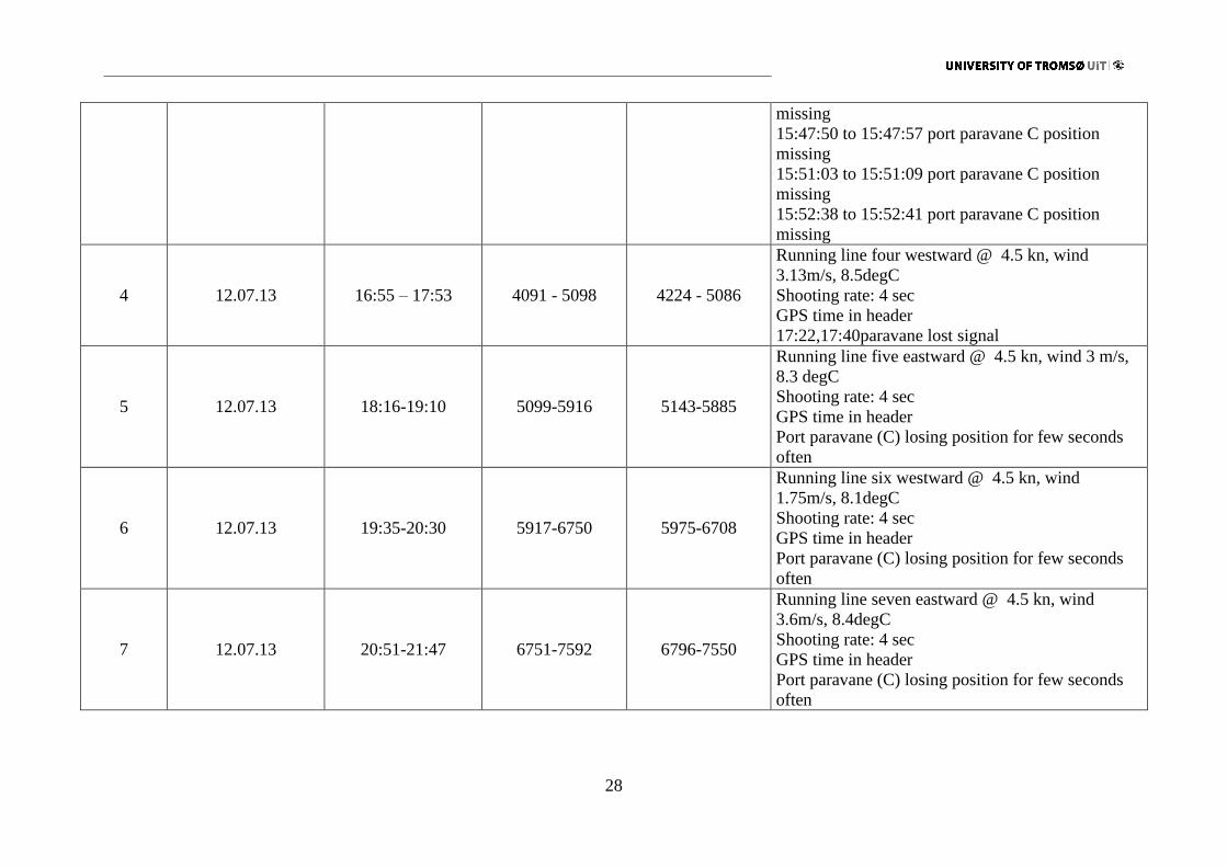
4 12.07.13 16:55 – 17:53 4091 - 5098 4224 - 5086
Running line four westward @ 4.5 kn, wind
3.13m/s, 8.5degC
Shooting rate: 4 sec
GPS time in header
17:22,17:40paravane lost signal
5 12.07.13 18:16-19:10 5099-5916 5143-5885
Running line five eastward @ 4.5 kn, wind 3 m/s,
8.3 degC
Shooting rate: 4 sec
GPS time in header
Port paravane (C) losing position for few seconds
often
6 12.07.13 19:35-20:30 5917-6750 5975-6708
Running line six westward @ 4.5 kn, wind
1.75m/s, 8.1degC
Shooting rate: 4 sec
GPS time in header
Port paravane (C) losing position for few seconds
often
7 12.07.13 20:51-21:47 6751-7592 6796-7550
Running line seven eastward @ 4.5 kn, wind
3.6m/s, 8.4degC
Shooting rate: 4 sec
GPS time in header
Port paravane (C) losing position for few seconds
often

29
8 12.07.13- 22:11-23:07 7593-8425 7632-8375
Running line eight westward @ 4.5 kn, wind 2 m/s,
8.4 degC
Shooting rate: 4 sec
GPS time in header
Port paravane (C) losing position for few seconds
often
9
12.07.13- 13.07.13 23:27 - 00:21 8426 - 9495 8461 - 9226
Running line nine eastward @ 4.5 kn, wind 3.6 m/s,
8.4 degC
Shooting rate: 4 sec
GPS time in header
Port paravane (C) losing position for few seconds
often
10 13.07.13 00:48 – 01:43 9496 - 10695 9625 - 10452
Running line ten westward @ 4.5 kn, wind 3.6 m/s,
8.4 degC
Shooting rate: 4 sec
GPS time in header
11 13.07.13 02:05 – 02:57 10696 - 11753 10757 - 11539
Running line eleven eastward @ 4.5 kn, wind 4.6
m/s, 8.4 degC
Shooting rate: 4 sec
GPS time in header
12 13.07.13 03:20 – 04:20 11754 - 13008 11871 - 12769
Running line twelve westward @ 4.0 kn, wind 4.7
m/s, 8.9 degC
Shooting rate: 4 sec
GPS time in header
13 13.07.13 04:41 – 05:36 13009 -14000 13070 - 13893
Running line thirteen eastward @ 4.4 kn, wind 7.2
m/s, 8.8 degC
Shooting rate: 4 sec
GPS time in header
This is a reshoot of line 1, same direction
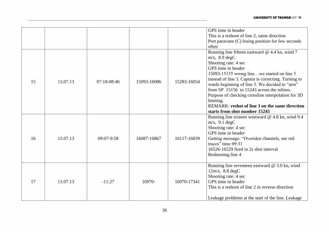
14 13.07.13 06:03-06:56 14296-15092 14326-15072
Running line fourteen westward @ 4.5 kn, wind 7
m/s, 9.1 degC
Shooting rate: 4 sec
30
GPS time in header
This is a reshoot of line 2, same direction
Port paravane (C) losing position for few seconds
often
15 13.07.13 07:18-08:46 15093-16086 15283-16054
Running line fifteen eastward @ 4.4 kn, wind 7
m/s, 8.9 degC
Shooting rate: 4 sec
GPS time in header
15093-15155 wrong line…we started on line 5
instead of line 3. Captain is correcting. Turning to
wards beginning of line 3. We decided to “arm”
from SP 15156 to 15243 across the inlines.
Purpose of checking crossline interpolation for 3D
binning.
REMARK: reshot of line 3 on the same direction
starts from shot number 15245
16 13.07.13 09:07-9:58 16087-16867 16117-16839
Running line sixteen westward @ 4.8 kn, wind 9.4
m/s, 9.1 degC
Shooting rate: 4 sec
GPS time in header
Getting message: “Overiden channels, see red
traces” time 09:31
16526-16529 fired in 2s shot interval
Reshooting line 4
17 13.07.13 -11:27 16970- 16970-17341
Running line seventeen eastward @ 3.0 kn, wind
12m/s, 8.8 degC
Shooting rate: 4 sec
GPS time in header
This is a reshoot of line 2 in reverse direction
Leakage problems at the start of the line. Leakage

31
unstable and varying. SPSU rebooted multiple
times. PC rebooted. Ship speed reduced to 3 kn.
Acquisition ok at about 2/3 into the line continuing
to see if failure re-appears.
No further problems until the end of line. Will try
turning and acquire the next line.
18 13.07.13 12:00-13:09 17842-19303 17891-18886
Running line eighteen westward @ 3.5 kn, wind
9.65m/s, 9 degC
Shooting rate: 4 sec
GPS time in header
Line 1 in reverse direction
19 13.07.13 13:45-14:52 19304-20443 19410-20414
Running line nineteen eastward @ 3.4kn, wind
11.5 m/s, 9 degC
Shooting rate: 4 sec
GPS time in header
This is line 2 reversed shot once again

32
Survey configuration:
Paravane wires @ 155 m
Signal cable @ 177 m Tensions are around 250-300 kg
1
2 3
4 5
6 7 8 9 10
11 12
13
14 Drop-lead: 6 m
A/D can: 0.3 m
Soilid state streamer: 25 m Channels: 8 Group spacing : 3.125 m
Offsets GPS to wire connection point
0-1 m
1-2 m
GPS
first channel: 1.5625 m

33
Observed spread of paravanes: 158-163 m
Observed distance between gun and paravanes: 93 – 103 m, deviations between distances to both paravanes up to 5 m
Gun system: mini-GI (15/15 in3)
Shooting pressure: ~160 bar
Shooting interval: 4 sec
Recording Length: 1.5 sec