use of the particle level set method for …web.stanford.edu/group/fpc/publications/enright...
TRANSCRIPT
USE OF THE PARTICLE LEVEL SET METHOD
FOR ENHANCED RESOLUTION OF
FREE SURFACE FLOWS
a dissertation
submitted to the program in
scientific computing and computational mathematics
and the committee on graduate studies
of stanford university
in partial fulfillment of the requirements
for the degree of
doctor of philosophy
Douglas Patrick Enright
August 2002

c© Copyright by Douglas Patrick Enright 2002
All Rights Reserved
ii
I certify that I have read this dissertation and that, in
my opinion, it is fully adequate in scope and quality as a
dissertation for the degree of Doctor of Philosophy.
Ronald P. Fedkiw(Computer Science)(Principal Advisor)
I certify that I have read this dissertation and that, in
my opinion, it is fully adequate in scope and quality as a
dissertation for the degree of Doctor of Philosophy.
Joel H. Ferziger(Mechanical Engineering)
I certify that I have read this dissertation and that, in
my opinion, it is fully adequate in scope and quality as a
dissertation for the degree of Doctor of Philosophy.
Juan J. Alonso(Aeronautics and Astronautics)
Approved for the University Committee on Graduate
Studies:
iii
Abstract
A new numerical method for improving the mass conservation properties of the level
set method when the interface is passively advected in a flow field is proposed. The
method, a hybrid “Particle Level Set Method”, uses Lagrangian marker particles to
rebuild a level set representation of the interface in regions which are under-resolved.
This is often the case for flows undergoing stretching and tearing. A level set only
approach towards maintaining small-scale interface features is subject to excessive
amounts of numerical regularization. This numerical regularization artificially al-
ters or destroy these features. By combining a simple Lagrangian method, massless
marker particles, with the level set method, the ability to smoothly represent both
large and small scale geometrical features is obtained while maintaining the imple-
mentation simplicity characteristic of the level set method. A variety of interface
tracking tests, including a newly proposed three dimensional deformation flow test
case, are performed to demonstrate that the method compares favorably with vol-
ume of fluid methods in the conservation of mass and purely Lagrangian schemes for
interface resolution.
The robustness of the method in representing complex, three dimensional free
surface fluid flows is illustrated through its use in producing physically based ani-
mations of the pouring of a glass of water; the splash generated by the impact of a
ball thrown into a tank of water; and the breaking of a wave on a submerged beach.
The behavior of the water is calculated by a three dimensional Navier-Stokes free sur-
face fluid simulation. A novel application of a level set based velocity extrapolation
technique is used to provide a smooth, physically based velocity field away from the
liquid at the interface. This velocity field satisfies the physical boundary conditions
iv

at the interface and provides a plausible velocity field for use by Lagrangian particles
outside the liquid as required by the “Particle Level Set Method”. Selected frames
from each of the animations are provided.
v

Acknowledgments
The material in this dissertation is drawn from two articles, “A Hybrid Particle
Level Set Method for Improved Interface Capturing” to appear in the Journal of
Computational Physics and “Animation and Rendering of Complex Water Surfaces”
published in the Proceedings of SIGGRAPH 2002.
Research supported in part by an ONR YIP and PECASE award N00014-01-1-
0620, the DOE ASCI Academic Strategic Alliances Program (LLNL contract B341491),
NSF DMS-0106694, and a Howard Hughes Doctoral Fellowship from the Hughes Air-
craft and Raytheon Systems Companies.
vi
Contents
Abstract iv
Acknowledgments vi
1 Introduction 1
1.1 Background . . . . . . . . . . . . . . . . . . . . . . . . . . . . . . . . 1
1.2 Curvature and Numerical Regularization . . . . . . . . . . . . . . . . 3
1.3 Scope and Presentation . . . . . . . . . . . . . . . . . . . . . . . . . . 7
2 Numerical Method 11
2.1 Level Set Method . . . . . . . . . . . . . . . . . . . . . . . . . . . . . 11
2.2 Massless Marker Particles . . . . . . . . . . . . . . . . . . . . . . . . 16
2.3 Particle Level Set Method . . . . . . . . . . . . . . . . . . . . . . . . 18
2.3.1 Initialization of Particles . . . . . . . . . . . . . . . . . . . . . 18
2.3.2 Time Integration . . . . . . . . . . . . . . . . . . . . . . . . . 20
2.3.3 Error Correction of the Level Set Function . . . . . . . . . . . 20
2.3.4 Reinitialization . . . . . . . . . . . . . . . . . . . . . . . . . . 23
2.3.5 Particle Reseeding . . . . . . . . . . . . . . . . . . . . . . . . 24
3 Examples 31
3.1 Rigid Body Rotation of Zalesak’s Disk . . . . . . . . . . . . . . . . . 31
3.2 Single Vortex . . . . . . . . . . . . . . . . . . . . . . . . . . . . . . . 33
3.3 Deformation Field . . . . . . . . . . . . . . . . . . . . . . . . . . . . . 35
3.4 Rigid Body Rotation of Zalesak’s Sphere . . . . . . . . . . . . . . . . 36
vii
3.5 Three Dimensional Deformation Field . . . . . . . . . . . . . . . . . . 38
4 Free Surface Calculations 54
4.1 Liquid Free Surface Flows . . . . . . . . . . . . . . . . . . . . . . . . 54
4.2 CFD and Computer Animation . . . . . . . . . . . . . . . . . . . . . 55
4.3 Liquid Model . . . . . . . . . . . . . . . . . . . . . . . . . . . . . . . 58
4.3.1 Navier-Stokes Equations . . . . . . . . . . . . . . . . . . . . . 58
4.3.2 Free Surface Boundary Conditions . . . . . . . . . . . . . . . . 59
4.4 Computational Method . . . . . . . . . . . . . . . . . . . . . . . . . . 60
4.4.1 Finite Difference Discretization . . . . . . . . . . . . . . . . . 60
4.4.2 Velocity Extrapolation Near Free Surface . . . . . . . . . . . . 62
4.4.3 Particle Level Set Interface Treatment . . . . . . . . . . . . . 64
4.4.4 Boundaries . . . . . . . . . . . . . . . . . . . . . . . . . . . . 65
4.4.5 Time Step Calculation . . . . . . . . . . . . . . . . . . . . . . 66
4.4.6 Overall Computational Cycle . . . . . . . . . . . . . . . . . . 66
4.5 Examples . . . . . . . . . . . . . . . . . . . . . . . . . . . . . . . . . 67
4.5.1 Rendering . . . . . . . . . . . . . . . . . . . . . . . . . . . . . 67
4.5.2 Pouring A Glass of Water . . . . . . . . . . . . . . . . . . . . 68
4.5.3 Splash Generated From Ball Impact . . . . . . . . . . . . . . . 69
4.5.4 Breaking Wave . . . . . . . . . . . . . . . . . . . . . . . . . . 70
5 Conclusions and Future Directions 86
Bibliography 89
viii

List of Tables
3.1 Zalesak’s disk. Level set method. . . . . . . . . . . . . . . . . . . . . 33
3.2 Zalesak’s disk. Particle level set method. . . . . . . . . . . . . . . . . 33
3.3 One period of vortex flow. Level set method. . . . . . . . . . . . . . . 35
3.4 One period of vortex flow. Particle level set method. . . . . . . . . . 35
3.5 One period of deformation flow. Level set method. . . . . . . . . . . . 36
3.6 One period of deformation flow. Particle level set method. . . . . . . 36
ix
List of Figures
1.1 Shrinking square. Initial interface location and velocity field. . . . . . 9
1.2 Shrinking square. Final interface location of the (correct) level set
solution. . . . . . . . . . . . . . . . . . . . . . . . . . . . . . . . . . . 9
1.3 Shrinking square. Passively advected particles are initially seeded in-
side the interface. . . . . . . . . . . . . . . . . . . . . . . . . . . . . . 10
1.4 Shrinking square. Final (incorrect) location of the passively advected
marker particles. . . . . . . . . . . . . . . . . . . . . . . . . . . . . . 10
2.1 Interface resolution with particles . . . . . . . . . . . . . . . . . . . . 17
2.2 Particle Level Set computational cycle. . . . . . . . . . . . . . . . . . 25
2.3 Expanding square. Initial interface location and velocity field. . . . . 28
2.4 Expanding square. Final interface location of the level set solution. . 28
2.5 Expanding square. Passively advected particles are initially seeded
inside the interface. . . . . . . . . . . . . . . . . . . . . . . . . . . . . 29
2.6 Expanding square. Final location the passively advected marker par-
ticles. . . . . . . . . . . . . . . . . . . . . . . . . . . . . . . . . . . . . 29
2.7 Expanding square. Location of interior particles after one application
of the reseeding algorithm. . . . . . . . . . . . . . . . . . . . . . . . . 30
3.1 Zalesak’s Disk. Initial placement of particles. . . . . . . . . . . . . . . 40
3.2 Zalesak’s Disk. Particle positions after the initial attraction step. . . 40
3.3 Zalesak’s Disk. Particle level set solution after one revolution. . . . . 41
3.4 Zalesak’s Disk. Comparison of level set, particle level set and theory
after one revolution. . . . . . . . . . . . . . . . . . . . . . . . . . . . 42
x

3.5 Zalesak’s Disk. Comparison of level set, particle level set and theory
after two revolutions. . . . . . . . . . . . . . . . . . . . . . . . . . . . 42
3.6 Zalesak’s Disk. Illustration of escaped particles after one revolution. . 43
3.7 Vortex Flow. Initial data and velocity field. . . . . . . . . . . . . . . 44
3.8 Vortex Flow. Comparison of the particle level set and front tracked
solutions at t = 1. . . . . . . . . . . . . . . . . . . . . . . . . . . . . . 45
3.9 Vortex Flow. Illustration of escaped particles at t = 1. . . . . . . . . 45
3.10 Vortex Flow. Comparison of the particle level set, level set, and front
tracked solutions at t = 3. . . . . . . . . . . . . . . . . . . . . . . . . 46
3.11 Vortex Flow. Comparison of the particle level set, level set, and front
tracked solutions at t = 5. . . . . . . . . . . . . . . . . . . . . . . . . 46
3.12 Vortex Flow. Error analysis of the time reversed flow level set solution
for grid sizes 642, 1282, and 2562. . . . . . . . . . . . . . . . . . . . . 47
3.13 Vortex Flow. Error analysis of the time reversed flow particle level set
solution for grid sizes 642, 1282, and 2562. . . . . . . . . . . . . . . . 47
3.14 Deformation Flow. Comparison of level set, particle level set, and front
tracked solutions at t = 1. . . . . . . . . . . . . . . . . . . . . . . . . 48
3.15 Deformation Flow. Error analysis of the time reversed flow level set
solution for grid sizes 642, 1282, and 2562. . . . . . . . . . . . . . . . 49
3.16 Deformation Flow. Error analysis of the time reversed flow particle
level set solution for grid sizes 642, 1282, and 2562. . . . . . . . . . . . 49
3.17 Zalesak’s sphere. Level set solution. . . . . . . . . . . . . . . . . . . . 50
3.18 Zalesak’s sphere. Particle level set solution. . . . . . . . . . . . . . . . 51
3.19 Deformation test case. Level set solution. . . . . . . . . . . . . . . . . 52
3.20 Deformation test case. Particle level set solution. . . . . . . . . . . . 53
4.1 Comparison of Hybrid Volume Model and the Particle Level Set method
for one rotation of Zalesak’s Disk . . . . . . . . . . . . . . . . . . . . 73
4.2 Velocity-Pressure (MAC) staggered grid arrangement . . . . . . . . . 74
4.3 Free Surface Overall Computational Cycle . . . . . . . . . . . . . . . 75
4.4 Free Surface Interface Evolution . . . . . . . . . . . . . . . . . . . . . 76
xi
4.5 Water being poured into a clear, cylindrical glass. . . . . . . . . . . . 77
4.6 Closeup of figure 4.5. . . . . . . . . . . . . . . . . . . . . . . . . . . . 78
4.7 Ball thrown into a tank of water. Hybrid Volume Model result. . . . 79
4.8 Ball thrown into a tank of water. Particle Level Set result. . . . . . . 80
4.9 Ball thrown into a tank of water. Formation of intial and secondary
splash sheets. . . . . . . . . . . . . . . . . . . . . . . . . . . . . . . . 81
4.10 Ball thrown into a tank of water. Secondary splash sheet and resulting
surface. . . . . . . . . . . . . . . . . . . . . . . . . . . . . . . . . . . 82
4.11 Two Dimensional Breaking Wave . . . . . . . . . . . . . . . . . . . . 83
4.12 Submerged Shelf . . . . . . . . . . . . . . . . . . . . . . . . . . . . . 83
4.13 Breaking Wave. Formation of initial plunging jet. . . . . . . . . . . . 84
4.14 Breaking Wave. Secondary splash up and bore creation phase. . . . . 85
xii
Chapter 1
Introduction
“It’s the pouring of milk into a glass.”
Jeffrey Katzenberg [33]
1.1 Background
The above response to a question concerning what was the single hardest shot in the
feature film “Shrek”, exemplifies the difficulty of the task that has faced the com-
putational fluid dynamics community over the past 50 years - to accurately simulate
complex, three dimensional liquid behavior. In order to obtain the degree of realism
required of engineering and computer graphics applications, the nonlinear phenom-
ena present in liquids needs to be modeled and simulated. This requires the use of
a three dimensional model of the behavior of liquids, the Navier-Stokes equations,
along with a moving boundary technique to handle the merging and pinching off of
liquid elements. Simulating these models on a computer also requires that appropri-
ate numerical methods are used to ensure that the results generated are faithful to
nature while at the same time incorporate a variety of practical engineering needs
including robustness, speed, and stability.
The need to capture complex topological features which can develop in three di-
mensional free surface flows is a serious constraint when considering what type of
moving boundary method to use to model the free surface. Purely Lagrangian flow
1
CHAPTER 1. INTRODUCTION 2
models, e.g. boundary integral and vortex methods [7, 37, 36, 48, 29, 19] suffer from
an inability to model changes in topology (pinching and merging) of the interface.
Utilizing a fixed grid representation for the flow variables (pressure, densities, veloci-
ties, etc.) can alleviate some of the difficulties mentioned above, but we are then faced
with the question of how to model the interface. A Lagrangian representation in the
spirit of Tryggvason et al. [92, 91] via particles placed on the interface and advected
by the flow can deal with arbitrary topologies, but at the cost of implementing and
verifying the correctness of complex algorithms required to rearrange the connectiv-
ity of particles in order to effect changes in topology. Marker particle based methods
[31, 15, 64, 16, 90] have a long history in modeling the motion of interfaces. These
methods avoid the geometrical complexities of connected front tracking algorithms,
but at the price of lacking a smooth, well defined interface. The interface can form
gaps and holes due to a lack of marker particle in cells which should be connected.
Also as noted in [15], careful consideration of the velocity boundary conditions to ap-
ply at the surface of the liquid is required in order to avoid introducing asymmetries
and other computational artifacts. Finally, both methods can require the use of arti-
ficial smoothing near the interface in order to obtain smooth geometrical quantities
[97].
A grid based Eulerian representation of the free surface avoids the many issues
inherent to Lagrangian schemes. Both Volume of Fluid (VOF) [34, 63] and the level
set method [60, 85] can easily support complex topologies. However, the use in VOF
of a single variable to represent the amount of liquid in a computational cell intro-
duces its own set of difficulties. In the attempt to maintain local mass conservation,
“blobby” flotsam and jetsam can spuriously appear [45], especially in under-resolved
regions of the flow due to excessive numerical surface tension being added to the sim-
ulation. Also, the reconstructed interface is not smooth or even continuous, lowering
the accuracy of the geometrical information (normals and curvature) at the interface
which can compromise the solution. Several researchers have worked to improve the
accuracy of the VOF geometrical information using convolution, see e.g. [94] and
[93].
On the other hand, the level set method use a function φ(~x, t) whose isocontour

CHAPTER 1. INTRODUCTION 3
φ = 0 is used to represent the interface. This function is advected by a flow field
given by ~u(~x, t). Mathematically, the evolution of the level set is given by
φt + ~u · ∇φ = 0. (1.1)
While level set methods have seen much success on a wide variety of problems
including fluid mechanics, combustion, computer vision, and materials science as
discussed in the recent review articles and books by Osher and Fedkiw [58, 59] and
Sethian [75, 74], their application to free surface flows has been problematic. As noted
in [85], the signed distance property of the initial level set function quickly ceases to
exist after a couple of time steps of equation 1.1, especially on coarse computational
grids. Since the interface is defined by a single isocontour of φ, the signed distance
property away from the interface is not required. However, accurate evolution of the
level set function which represents a contact discontinuity is severely impaired if the
gradient of φ is not smooth. How the level set method deal with this issue and how to
create a numerical method which corrects for this built in characteristic of the level
set method, is a key issue that will be addressed in this work.
1.2 Curvature and Numerical Regularization
The great success of level set methods (and other Eulerian methods) can be attributed
to the role of curvature in numerical regularization which allows the proper vanishing
viscosity solution to be obtained. This regularization of the level set function allows
the method to handle changes in topology in a natural manner. The connection
between curvature and the notion of entropy conditions and shocks for hyperbolic
conservation laws was explored by Sethian [70, 71]. No Lagrangian scheme, including
discretization of the interface by marker particles, can achieve a similar result since
there is no a priori way to build regularization into the method. Lagrangian particles
faithfully follow the characteristics of the flow, but must be deleted (usually “by
hand”) if the characteristics merge.
The ability to identify and delete merging characteristics is clearly seen in a purely
CHAPTER 1. INTRODUCTION 4
geometrically driven flow in which a curve is advected normal to itself at constant
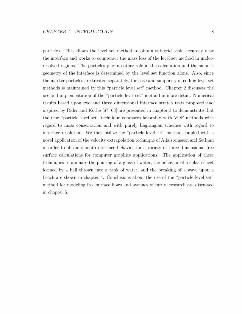
speed. Figure 1.1 shows an initially square interface taken as the φ = 0 isocontour
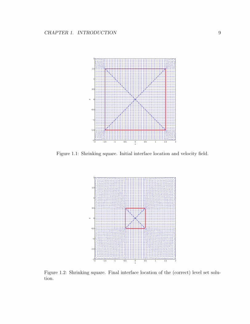
of a level set function along with the associated velocity field defined by ∇φ/|∇φ|.This flow field has merging characteristics on the diagonals of the square. Figure
1.2 shows that a numerical solution computed using the level set method correctly
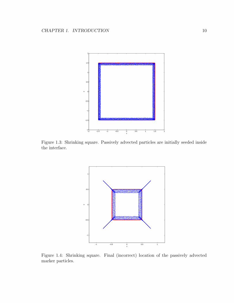
shrinks the box as time increases. On the other hand, a Lagrangian front tracking
model of the interface will not calculate the correct motion. We demonstrate this
by seeding passively advected particles interior to the zero isocontour of the level set
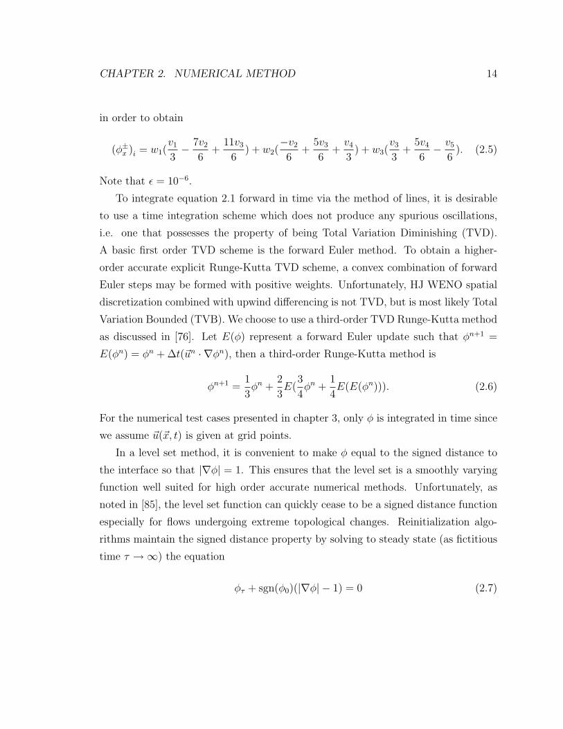
function as shown in figure 1.3. As the particle positions evolve in time, they follow
the characteristic velocities of the flow field as shown in figure 1.4. The particles
incorrectly form long, slender filaments on the diagonals of the square where charac-
teristics merge that should be deleted (as is correctly done by the level set method).
Helmsen [32] and others have used “de-looping” procedures in an attempt to remove
these incorrect particle tails. While these procedures are sometimes manageable in
two spatial dimensions, they become intractable in three spatial dimensions.
Despite a lack of explicit enforcement of conservation, Lagrangian schemes are
quite successful in conserving mass since they preserve material advected along char-
acteristics for all time as opposed to regularizing mass out of existence as Eulerian
front capturing methods may do. For under-resolved flows, Eulerian capturing meth-
ods can not accurately tell if characteristics merge, separate, or are parallel. This
indeterminacy can cause level set methods to calculate weak solutions and delete
characteristics when they appear to be merging. Osher and Sethian [60] constructed
the level set method to deal with the case in which characteristics do merge as seen in
figure 1.2, i.e. to recognize the presence of shocks and delete merging characteristic
information. We are faced with the difficult question of the appropriateness of using
level set schemes that merge characteristics automatically when we lack knowledge
about the characteristic structure in under-resolved regions of the flow. Moreover,
in the case of incompressible fluid flows, we know a priori that there are no shocks
present in the velocity field, and thus characteristic information should never be
deleted.
An Eulerian analysis can yield some insight into a possible solution to this problem.

CHAPTER 1. INTRODUCTION 5
If we use an upwind spatial discretization of equation 1.1 along with a first order
temporal discretization, we obtain (in one spatial dimension)
φn+1i − φn
i
∆t+ un
i (D±φ)ni = 0, (1.2)
where D±φ is a forward/backward difference of φ,
(D+φ)ni =
φni+1 − φn
i
∆x,
(D−φ)ni =
φni − φn
i−1
∆x.
Which difference to take is determined by the sign of uni according to the method of
characteristics. For uni > 0, we choose D−φ since information is flowing from left to
right and D+φ for uni < 0. What is of more interest is the numerical error associated
with the spatial discretization of equation 1.2. To lowest order in ∆x, the error term
is
±∆x
2
(∂2φ
∂x2
)n
i
+ O(∆x2). (1.3)
In higher dimensions on an equally spaced grid, this error term is ε4φ, with ε ∼ ∆x.
Since this term is an inherent part of our calculation, if we substitute the exact
solution of equation 1.1, Φ, into our finite difference approximation, we obtain
Φn+1i − Φn
i
∆t+ un
i (D±Φ)ni = ±∆x
2
(∂2Φ
∂x2
)n
i
, (1.4)
which is accurate to O(∆x). As ∆x → 0, the finite difference solution φni → Φ(~x, t)
in the sense that φni is a vanishing viscosity solution to equation 1.1. The smoothing
viscosity-like term on the right hand side of equation 1.4 provides a way to regularize
the solution obtained by the level set method in order to deal with shocks which form
due to changes in the topology of the interface. However, if ∆x is not sufficiently
small and/or we are trying to resolve features on the order of O(∆x), then the right
hand side of equation 1.4 does not approach zero. In this case (which is unfortunately
a common occurrence in many interesting interfacial flow problems) we are left with
CHAPTER 1. INTRODUCTION 6
a solution to equation 1.4, a convection-diffusion equation, rather than the solution
our original advection equation. If φ is a signed distance function, then the diffusion
present in equation 1.4 is proportional to the curvature of the interface. Regions of
high curvature relative to the grid size will experience the most diffusion.
The difficulties of using the level set method to capture contact discontinuities has
been brought to light by a series of test problems proposed by Rider and Kothe [67,
68]. These problems either contain large vortical flow components, inducing the
formation of under-resolved regions of the interface, or the interface possesses regions
of extremely high curvature, e.g. corners, which should be preserved during a rigid
body movement of the interface. By comparing various Lagrangian and Eulerian
methods for these flows, Rider and Kothe found that Lagrangian tracking schemes
maintain filamentary interface structures better than their Eulerian counterparts.
In the same study, it was noted that when fluid filaments become too thin to be
adequately resolved on the grid, level set methods lose (or gain) mass while VOF
methods form “blobby” filaments that locally enforce mass conservation but in the
process artificially move the interface. Both types of errors decrease the accuracy
of the interface location. The loss (or gain) of mass by level set methods can be
attributed to the diffusion present in equation 1.4 in an Eulerian sense or the incorrect
merging (or creation) of characteristics in a Lagrangian sense.
Attempts to improve mass conservation in level set methods have led to a variety
of Eulerian based methods. As noted earlier, Sussman et al. [85] recognized this
problem and proposed to reinitialize φ in order to maintain a smooth level set function.
While this method did improve the spatial discretization properties of φ, it did not
directly address the issue of under-resolved regions/regions of high curvature. Further
improvements to this reinitialization method by Sussman and Fatemi [83, 84] include
the introduction of a Lagrange multiplier constraint which attempts to preserve mass
on a cell-by-cell basis. Higher order ENO/WENO [39] approximations for the spatial
derivatives in the convection and reintialization steps have been proposed. Although
the use of higher order spatial approximations does indeed help conserve mass, as
shown in chapter 3, in regions where the level set senses that shocks are occurring
and applies numerical regularization to the interface, the accuracy of the interface
CHAPTER 1. INTRODUCTION 7
decreases to first order. We are then left with situation discussed earlier. Cheng et
al. [13], addressed the curvature-based diffusion present in level set methods through
the use of an anti-diffusive reinitialization scheme. The method attempts to move the
level set in a manner to recover the amount of area/volume lost during a time step.
An alternative approach to reinitialization has been proposed by Adalsteinsson and
Sethian [2]. In this scheme one smoothly extrapolates the velocity of the interface
away from the interface and moves φ according to this “extension velocity”. In many
level set applications this is a required procedure, since no velocity exists off the
interface. In the case of fluid flows however, the fluid velocity is a valid “extension
velocity”. However, in under-resolved regions this scheme requires the use of suspect
geometrical information contained in the level set function. Finally, Sussman and
Puckett [80] combined VOF and level set methods in order to alleviate some of the
problems of the VOF method. The resulting scheme is completely Eulerian in nature
and does not incorporate any of the front-tracked characteristic information needed
in under-resolved regions. Instead, the VOF local mass constraint is still blindly
applied. The level set method is only used as a smoother in order to obtain better
approximations of the curvature of the interface than is possible with VOF methods.
None of these methods take advantage of the underlying characteristic flow field
information that Lagrangian interface methods successfully utilize.
1.3 Scope and Presentation
In this dissertation, we propose a new method which combines the best properties of
an Eulerian level set method and a marker particle Lagrangian scheme. Our method
randomly places a set of marker particles near the interface (defined by the zero level
set) and allows them to passively advect with the flow. In fluid flows, particles do
not cross the interface except when the interface capturing scheme fails to accurately
identify the interface location. If marker particles initially seeded on one side of the
interface are detected on the opposite side, this indicates an error in the level set
representation of the interface. We fix these errors by locally rebuilding the level
set function using the characteristic information present in these escaped marker
CHAPTER 1. INTRODUCTION 8
particles. This allows the level set method to obtain sub-grid scale accuracy near
the interface and works to counteract the mass loss of the level set method in under-
resolved regions. The particles play no other role in the calculation and the smooth
geometry of the interface is determined by the level set function alone. Also, since
the marker particles are treated separately, the ease and simplicity of coding level set
methods is maintained by this “particle level set” method. Chapter 2 discusses the
use and implementation of the “particle level set” method in more detail. Numerical
results based upon two and three dimensional interface stretch tests proposed and
inspired by Rider and Kothe [67, 68] are presented in chapter 3 to demonstrate that
the new “particle level set” technique compares favorably with VOF methods with
regard to mass conservation and with purely Lagrangian schemes with regard to
interface resolution. We then utilize the “particle level set” method coupled with a
novel application of the velocity extrapolation technique of Adalsteinsson and Sethian
in order to obtain smooth interface behavior for a variety of three dimensional free
surface calculations for computer graphics applications. The application of these
techniques to animate the pouring of a glass of water, the behavior of a splash sheet
formed by a ball thrown into a tank of water, and the breaking of a wave upon a
beach are shown in chapter 4. Conclusions about the use of the “particle level set”
method for modeling free surface flows and avenues of future research are discussed
in chapter 5.
CHAPTER 1. INTRODUCTION 9
−2 −1.5 −1 −0.5 0 0.5 1 1.5 2−2
−1.5
−1
−0.5
0
0.5
1
1.5
2
x
y
Figure 1.1: Shrinking square. Initial interface location and velocity field.
−2 −1.5 −1 −0.5 0 0.5 1 1.5 2−2
−1.5
−1
−0.5
0
0.5
1
1.5
2
x
y
Figure 1.2: Shrinking square. Final interface location of the (correct) level set solu-tion.
CHAPTER 1. INTRODUCTION 10
−2 −1.5 −1 −0.5 0 0.5 1 1.5 2−2
−1.5
−1
−0.5
0
0.5
1
1.5
2
x
y
Figure 1.3: Shrinking square. Passively advected particles are initially seeded insidethe interface.
−1 −0.5 0 0.5 1
−1
−0.5
0
0.5
1
x
y
Figure 1.4: Shrinking square. Final (incorrect) location of the passively advectedmarker particles.

Chapter 2
Numerical Method
“I think it [interface tracking] is a subject worthy of agreat deal of effort on its own; although it appearsalmost trivial, it really isn’t, and it really ought tobe done well, once and for all, if that is possible.”
R. DeBar [21]
2.1 Level Set Method
The underlying idea behind level set methods is to embed an interface Γ in R3 which
bounds an open region Ω ⊂ R3 as the zero level set of a higher dimensional function
φ(~x, t). The level set function has the following properties,
φ(~x, t) > 0 for ~x ∈ Ω
φ(~x, t) ≤ 0 for ~x 6∈ Ω,
where we include φ = 0 with the negative φ values so that it is not a special case. The
interface lies between φ > 0 and φ = 0, but can of course be identified as φ = 0. Note
that φ is a scalar function in R3 which greatly reduces the complexity of describing
the interface, especially when undergoing topological changes such as pinching and
merging.
The motion of the interface is determined by a velocity field, ~u, which can depend
11

CHAPTER 2. NUMERICAL METHOD 12
on a variety of things including position, time, geometry of the interface, or be given
externally, for instance as the material velocity in a fluid flow simulation. In most of
the examples below, the velocity field is externally given, and the evolution equation
for the level set function is given by
φt + ~u · ∇φ = 0. (2.1)
This equation only needs to be solved locally near the interface, e.g. see [1, 62].
Both φ and ~u = (u, v, w) are represented on a fixed Cartesian grid with a constant
grid spacing of ∆x = ∆y = ∆z. We use a dimension by dimension approach in
discretizing ~u · ∇φ = uφx + vφy + wφz term in equation 2.1. For the sake of brevity,
we proceed by discussing only the discretization of uφx. At a specific grid point,
xi, we choose either a left-sided or right-sided discretization of φx according to the
local velocity at xi. This corresponds to discretizing equation 2.1 according to the
method of characteristics. For ui < 0, we take φx = φ+x and for ui > 0, we take
φx = φ−x . Since level set methods appear to be sensitive to the accuracy used in
discretizing the spatial derivatives, we used a fifth order accurate Hamilton-Jacobi
WENO scheme [39] to calculate right and left biased derivatives, φ+x and φ−x , needed
by the method of characteristics.
To find φ−x , set
v1 =φi−2 − φi−3
∆x, v2 =
φi−1 − φi−2
∆x
v3 =φi − φi−1
∆x, v4 =
φi+1 − φi
∆x
v5 =φi+2 − φi+1
∆x
and to find φ+x , set
v1 =φi+3 − φi+2
∆x, v2 =
φi+2 − φi+1
∆x
v3 =φi+1 − φi
∆x, v4 =
φi − φi−1
∆x

CHAPTER 2. NUMERICAL METHOD 13
v5 =φi−1 − φi−2
∆x.
We utilize these first order divided differences to obtain three different polynomial
approximations of φ±x ,
φ1x =
v1
3− 7v2
6+
11v3
6(2.2)
φ2x =
−v2
6+
5v3
6+
v4
3(2.3)
φ3x =
v3
3+
5v4
6− v5
6. (2.4)
Essentially Non-Oscillatory (ENO) methods choose one of the above three approx-
imations. The choice of which approximation to use is made according to which
approximation generates the smoothest possible polynomial interpolation of φ. This
choice will hopefully approximate φ±x with the least error. For Weighted ENO meth-
ods, a weighted convex combination of equations 2.2- 2.4 is used. The weights
w1, w2, and w3, are calculated using an estimate of the smoothness of each stencil.
These smoothness estimates are given by
S1 =13
12(v1 − 2v2 + v3)
2 +1
4(v1 − 4v2 + 3v3)
2
S2 =13
12(v2 − 2v3 + v4)
2 +1
4(v2 − v4)
2
S3 =13
12(v3 − 2v4 + v5)
2 +1
4(3v3 − 4v4 + v5)
2
and the weights by
a1 =1
10
1
(ε + S1)2, w1 =
a1
a1 + a2 + a3
a2 =6
10
1
(ε + S2)2, w2 =
a2
a1 + a2 + a3
a3 =3
10
1
(ε + S3)2, w3 =
a3
a1 + a2 + a3
CHAPTER 2. NUMERICAL METHOD 14
in order to obtain
(φ±x )i = w1(v1
3− 7v2
6+
11v3
6) + w2(
−v2
6+
5v3
6+
v4
3) + w3(
v3
3+
5v4
6− v5
6). (2.5)
Note that ε = 10−6.
To integrate equation 2.1 forward in time via the method of lines, it is desirable
to use a time integration scheme which does not produce any spurious oscillations,
i.e. one that possesses the property of being Total Variation Diminishing (TVD).
A basic first order TVD scheme is the forward Euler method. To obtain a higher-
order accurate explicit Runge-Kutta TVD scheme, a convex combination of forward
Euler steps may be formed with positive weights. Unfortunately, HJ WENO spatial
discretization combined with upwind differencing is not TVD, but is most likely Total
Variation Bounded (TVB). We choose to use a third-order TVD Runge-Kutta method
as discussed in [76]. Let E(φ) represent a forward Euler update such that φn+1 =
E(φn) = φn + ∆t(~un · ∇φn), then a third-order Runge-Kutta method is
φn+1 =1
3φn +
2
3E(
3
4φn +
1
4E(E(φn))). (2.6)
For the numerical test cases presented in chapter 3, only φ is integrated in time since
we assume ~u(~x, t) is given at grid points.
In a level set method, it is convenient to make φ equal to the signed distance to
the interface so that |∇φ| = 1. This ensures that the level set is a smoothly varying
function well suited for high order accurate numerical methods. Unfortunately, as
noted in [85], the level set function can quickly cease to be a signed distance function
especially for flows undergoing extreme topological changes. Reinitialization algo-
rithms maintain the signed distance property by solving to steady state (as fictitious
time τ →∞) the equation
φτ + sgn(φ0)(|∇φ| − 1) = 0 (2.7)

CHAPTER 2. NUMERICAL METHOD 15
where sgn(φ0) is a one-dimensional smeared sign function that is approximated nu-
merically in [85] as
sgn(φ0) =φ0√
φ20 + (∆x)2
.
Efficient ways to solve equation 2.7 to steady state via fast marching methods are
discussed in [72]. However, while it is possible to construct second order accurate
marching methods as discussed in [73], these methods become increasingly problem-
atic due to the need to use higher order accurate interpolants to initialize the function
on the band of grid points surrounding the φ = 0 isocontour. For the current state of
the art concerning fast marching method solutions to equation 2.7 we refer the reader
to [17].
For the purposes of calculating a second order accurate distance function near the
interface while avoiding the computational difficulties discussed above, we perform
10 iterations of equation 2.7 in a narrow band (10 grid cells) about φ = 0. At
the same time we perform a first order fast marching method over the entire grid.
Outside the narrow band, we use the value of φ calculated by the fast marching
method while inside the narrow band we use the value calculated via equation 2.7
unless it differs from the fast marching solution by more than max(∆x, ∆y, ∆z).
In this case, we choose the value obtained by the fast marching method. We also
prevent φ from changing sign during the reinitialization process and use a fifth order
accurate Hamilton-Jacobi WENO scheme as described above to calculate the spatial
derivatives in equation 2.7.
Geometrical quantities can be calculated from the level set function, including the
unit normal to the interface,
~N =∇φ
|∇φ| , (2.8)
and the curvature,
κ = ∇ ·( ∇φ
|∇φ|)
. (2.9)
The spatial derivatives in equations 2.8 and 2.9 can be calculated using standard
second order accurate central differencing when the denominators are non-zero. When
|∇φ| = 0 one-sided differencing is used.
CHAPTER 2. NUMERICAL METHOD 16
2.2 Massless Marker Particles
Two sets of massless but finite size marker particles are placed near the interface
with one set, the positive particles, in the φ > 0 region and the other set, the nega-
tive particles, in the φ ≤ 0 region. It is unnecessary to place particles far from the
interface since the sign of the level set function easily identifies these regions. This
greatly reduces the number of particles needed in a simulation. Traditional marker
particle schemes [31, 66] place particles throughout the domain, although Amsden [5]
proposed a method that only requires particles near the surface. More recently, Chen
et al. [16] introduced a marker particle method which uses only particles placed on
the surface. The lack of connectivity information between the particles differenti-
ates these methods from the connected front-tracking approaches by Tryggvason and
collaborators [92, 91].
The particles are advected using the evolution equation,
d~xp
dt= ~u(~xp), (2.10)
where ~xp is the position of the particle and ~u(~xp) is its velocity. The particle velocities
are trilinearly interpolated from the velocities on the nearest grid points. This trilinear
interpolation limits the particle evolution to second order accuracy. While it is not
difficult to implement higher order accurate interpolation schemes (with appropriate
limiters), we have found trilinear interpolation to be sufficient and prefer it for its
efficiency. We use the grid velocity at time n, although the velocity at time n+1 could
be used as well. A third order accurate TVD Runge-Kutta method (equation 2.6) is
used to evolve the particle positions forward in time.
The particles are used to both track characteristic information and to reconstruct
the interface in regions where the level set method fails to accurately preserve mass.
For the purpose of interface reconstruction, we allow the particles to overlap as il-
lustrated in the bottom of figure 2.1. This allows us to reconstruct the interface
exactly as the number of particles approaches infinity. Non-overlapping spheres will
not accomplish this. For example, the top of figure 2.1 shows how three equally sized

CHAPTER 2. NUMERICAL METHOD 17
Three Non-Overlapping Circles
Six Overlapping Circles
Figure 2.1: The top picture shows how three equally sized non-overlapping circlesleave large spaces when attempting to represent a straight line interface, while thebottom picture shows how six equally sized overlapping circles more readily resolvethe line.
non-overlapping circles leave large spaces when used to represent a straight inter-
face, while the bottom of the figure shows that six equally sized overlapping circles
more readily resolve the line. Since the particles are not physical, allowing them to
overlap does not create any inconsistency in the method. The particles are used to
track characteristic information, and allowing overlap merely means that some of the
characteristic information is duplicated. Since the particles are allowed to overlap at
the end of the time step as well, carrying around duplicate characteristic information
does not hinder the scheme in any way.
For the purpose of interface reconstruction, a sphere of radius rp is centered at
each particle location, ~xp. The radius of each particle is bounded by minimum and
maximum values based upon the grid spacing. Maximum and minimum radii which
appear to work well are
rmin = .1 min(∆x, ∆y, ∆z) (2.11)
rmax = .5 min(∆x, ∆y, ∆z). (2.12)

CHAPTER 2. NUMERICAL METHOD 18
This allows multiscale sampling of the interface by the particles. This particular choice
of bounds on the particle radii (from 10% to 50% of a grid cell) was the first one we
tried; further experimentation might give improved results. However, as shown in the
examples section, these bounds give surprisingly good results. The reconstruction of
the interface utilizing both particle and level set information is given in section 2.3.3.
We use an array based implementation to store the particle information, since
connectivity information is not required. This simplifies the integration of the parti-
cle evolution equation 2.10. Certain performance optimizations of the particle array
storage can be made, depending on the frequency of particle insertions and deletions.
For example, one can use an oversized particle array which supports additional inser-
tions without resizing as well as a list of the indices of valid particles so that constant
repacking of the array can be avoided.
2.3 Particle Level Set Method
2.3.1 Initialization of Particles
Initially particles of both sign are randomly placed in cells that have at least one corner
within 3 max(∆x, ∆y, ∆z) of the interface, i.e. for a given cell, we check whether
|φ| < 3 max(∆x, ∆y, ∆z) at any of the eight corners. The number of particles of each
type (positive or negative) per cell is set to a default of 64 particles (16 in 2D, or 4
in 1D, i.e. 4 particles per spatial dimension), although this number is user definable.
An example of this initial particle seeding is shown in figure 3.1.
After the initial seeding, the particles are attracted to the correct side of the
interface (i.e. positive particles to the φ > 0 side and negative particles to the φ ≤ 0
side) into a band between a distance of bmin = rmin (the minimum particle radius)
and bmax = 3 max(∆x, ∆y, ∆z) of the interface. The thickness of the particle bands
on each side of the interface, 3 max(∆x, ∆y, ∆z) was the first we tried. One may use
thinner particle bands in order to obtain better computational performance, with the
caveat that this method will revert to a level set only method in regions which do not
possess an adequate particle resolution of the interface. The original seeding of the
CHAPTER 2. NUMERICAL METHOD 19
particles generates a random distribution of particles in the direction tangent to the
interface. In order to obtain a random distribution of the particles in the direction
normal to the interface, we chose an isocontour φgoal ∈ (±bmin,±bmax) using a uniform
random distribution. Then we carry out an attraction step with the aim of placing
the particle on the φ = φgoal level set contour.
The particles are attracted to the appropriate isocontours taking advantage of
geometrical information contained within the level set function φ. Near the interface,
the normal vectors give the direction to the nearest point on the interface. To attract
a particle at ~xp with a current interpolated level set value of φ(~xp) to the φ = φgoal
level set contour along the shortest possible path, one calculates
~xnew = ~xp + λ(φgoal − φ(~xp)) ~N(~xp), (2.13)
with λ = 1. For under-resolved regions or regions where the quality of the geometric
information contained within the level set function has been degraded, equation 2.13
may not put the particle on the desired contour or even in the appropriate band.
To overcome these difficulties, several iterations of this scheme may be needed. If
equation 2.13 places a particle outside the computational domain, λ is halved. Then,
if equation 2.13 (with this new λ) puts the particle in the appropriate band, i.e.
(±bmin,±bmax), we accept the new particle position even though it may not be on
the φ = φgoal contour. Otherwise, we halve λ once more, determine the new particle
position and repeat the process with λ again initially set to 1 and ~xp set to this newly
calculated position. If, after a preset maximum number of iterations (e.g. we use
15), the particle is still not within the desired band, it is deleted. Figure 3.2 shows
Zalesak’s disk after the particle attraction step has been completed. While there are
a number of particle placement strategies that could be used to accurately sample the
cell including just placing the particles on their respective sides of the interface, e.g.
see [27] for a discussion of ”jitter”, the technique discussed above worked surprisingly
well as can be seen in the examples section. However, the use of more sophisticated
techniques might improve the numerical results.

CHAPTER 2. NUMERICAL METHOD 20
Finally, each particle radius is set according to
rp =
rmax if spφ(~xp) > rmax
spφ(~xp) if rmin ≤ spφ(~xp) ≤ rmax
rmin if spφ(~xp) < rmin,
(2.14)
where sp is the sign of the particle (+1 for positive particles and -1 for negative
particles). This equation adjusts the particle size such that the boundary of the
particle is tangent to the interface whenever possible, while adhering to the restriction
that the particle radius is bounded by rmin and rmax.
2.3.2 Time Integration
The marker particles and the level set function are separately integrated forward in
time utilizing the third order accurate TVD Runge-Kutta method previously dis-
cussed. Separate temporal integration allows for the possibility of using a different
ordinary differential equation solver for the particle evolution, even though we have
not done so here.
2.3.3 Error Correction of the Level Set Function
The error correction of the level set function by the two sets of particles is comprised
of several steps: the identification by the particles of where errors in the interface rep-
resentation by the level set are occurring; calculation by each particle of the amount
of error present; the combining of all of the individual particle contributions to form a
reduced error representation of φ. Each of these steps will be discussed in more detail
below. Also, we note that we apply the error correction step after each modification
of the level set as shown in figure 4.3.
Identification of Error: After each complete Runge-Kutta cycle, the particles are
used to locate possible errors in the level set function due to the non-physical deletion
of (incorrectly perceived) merging characteristics. Particles that are on the wrong side
of the interface by more than their radius, as determined by the local interpolated

CHAPTER 2. NUMERICAL METHOD 21
φ(~xp), are considered to have escaped. Escaped particles indicate that characteristics
have probably been incorrectly merged through regularization i.e. the level set method
has computed a weak solution. While not done for the examples shown in chapter 3,
since these weak solutions are locally only first order accurate one could experiment
with using a relatively low order accurate method for both the particle evolution and
the particle correction algorithms (less accurate than the fifth order accurate WENO
method used for the evolution of the level set function), due to the information
provided by the lagrangian particles. This information may improves the quality of
the computed results, since the particles provide characteristic information that was
discarded by the level set function. Moreover, lower order accurate methods are more
efficient to implement, decreasing the computational overhead.
In smooth, well resolved, regions of the flow where the level set method is highly
accurate, the particles do not drift far across the interface, allowing us to retain the
high order accurate level set solution. A particle is not defined as escaped when
some portion of it crosses the interface. Otherwise, escaped particles would appear
all the time due to numerical errors (including roundoff error). If we allowed small
errors to force particle reconstruction of the level set function, we would need high
order accuracy for the particle evolution and correction methods. Instead, we define
a particle as escaped only when all of it crosses the interface. Since the particle radius
is O(∆x), error identification occurs only when the particle solution and the level set
solution differ to first order accuracy. With at least second order accurate evolution
methods for the particles and the level set function, one would not expect error
identification in well resolved regions of the flow. However, in under-resolved regions
where the level set method generates a first order accurate weak solution, second
order accurate particle evolution will identify errors in the level set representation of
the interface that need to be repaired. While one can change the escape condition for
the particles, we have found that the current choice produces good numerical results.
Quantification of Error: The spheres associated with each particle can be thought
of as locally defined level set functions. We represent the sphere centered at each
CHAPTER 2. NUMERICAL METHOD 22
particle using a level set function
φp(~x) = sp(rp − |~x− ~xp|) (2.15)
where sp is the sign of the particle, i.e ±1. The zero level set of φp corresponds to the
boundary of the particle sphere. The particle defined level set function is computed
locally on the eight corners of the cell containing the particle. The local values of φp
are the particle predictions of the values of the overall level set function, φ, on the
corners of the cell. Any variation of φ from φp indicates possible errors in the level
set solution.
Reduction of Error: We use the escaped positive particles to rebuild the φ > 0
region and the escaped negative particles to rebuild the φ ≤ 0 region. For example,
consider the φ > 0 region and an escaped positive particle. The values of φp at the
eight corners of the cell containing the particle are calculated using equation 2.15.
Each φp is compared to the local value of φ and the maximum of the two values is
taken as φ+. This is done for all escaped positive particles creating a reduced error
representation of the φ > 0 region. That is, given a level set φ and a set of escaped
positive particles E+, we initialize φ+ with φ and then calculate
φ+ = max∀p∈E+
(φp, φ+). (2.16)
Similarly, to calculate a reduced error representation of the φ ≤ 0 region, we initialize
φ− with φ and then calculate
φ− = min∀p∈E−
(φp, φ−). (2.17)
φ+ and φ− will not agree due to the errors in both the particle and level set methods
as well as interpolation errors, etc. We merge φ+ and φ− back into a single level set

CHAPTER 2. NUMERICAL METHOD 23
by setting φ equal to φ+ or φ−, whichever is less in magnitude at each grid point,
φ =
φ+ if |φ+| ≤ |φ−|φ− if |φ+| > |φ−|.
(2.18)
The minimum magnitude is used to reconstruct the interface (instead of, for example,
taking an average), since it gives priority to values that are closer to the interface.
Note that if the particle locations (from the particle evolution equation) are cal-
culated to second order accuracy and the O(∆x) escape condition is used, the error
reduction step is needed only in regions where the level set method has computed a
weak solution and deleted characteristics. Therefore, the accuracy requirements of
the error reduction step can be rather low while producing markedly improved numer-
ical results as the examples will show. While higher order accurate error reduction
methods might produce better results, there is a trade off against efficiency, especially
when the number of particles is large.
2.3.4 Reinitialization
Since the particle level set method relies on φ being an approximate signed distance
function, we reinitialize the level set function using equation 2.7 after each combined
Runge-Kutta cycle and error correction step. Unfortunately, reinitialization may
cause the zero level set to move, which is not desirable, so we use the particle level
set method to correct these errors as well.
During the reinitialization step information flows away from the φ = 0 isocontour.
This can be clearly seen by rewriting equation 2.7 as
φτ + ~v · ∇φ = sgn(φ0), (2.19)
where
~v = sgn(φ0)∇φ
|∇φ| .
Since the normal to the interface is given by ∇φ/|∇φ|, we see that equation 2.19 is
a nonlinear hyperbolic equation with characteristics determined by ~v, which point

CHAPTER 2. NUMERICAL METHOD 24
outwards from the interface. During the reinitialization step, we do not want the
particles to follow the characteristics associated with equation 2.19, rather we keep
the particles stationary. We then use the particles to identify and correct any errors
produced by the reinitialization scheme.
After reinitialization of the level set function, including the identification and
reduction of errors using particles, we adjust the radii of the particles according to
the current value of φ(~xp) according to equation 2.14. This radius adjustment feeds
information from the level set back to the particles, in an effort to ensure that a
consistent representation of the interface by the particles and the level set function
is maintained. In under-resolved regions, particles may jump (possibly relatively
far) across the interface in a single time step as the level set method computes a
weak solution, thereby deleting a large region of characteristic information. Through
the error correction steps outline above, these first order errors can be detected and
corrected for. By not deleting particle which remain escaped after each time step
or allowing their radii to become zero during the radii adjustment step, information
concerning any regions of deleted characteristic information is still maintained and
can be incorporated by the level set function on succeeding time steps.
In summary, the order of operations is: evolve both the particles and the level
set function forward in time, correct errors in the level set function using particles,
apply reinitialization, again correct errors in the level set function using particles, and
finally adjust the particle radii as illustrated in figure 2.2.
2.3.5 Particle Reseeding
In flows with interface stretching and tearing, regions which lack a sufficient number
of particles will form. This problem has also been observed in particle-only methods
which seed particles everywhere in the computational domain [30]. In order to accu-
rately resolve the interface for all time, we need to periodically readapt the particle
distribution to the deformed interface. The idea of adding and deleting particles has
been proposed by many authors, see for example [46]. We not only add and delete
particles in cells near the interface, but also delete particles that have drifted too
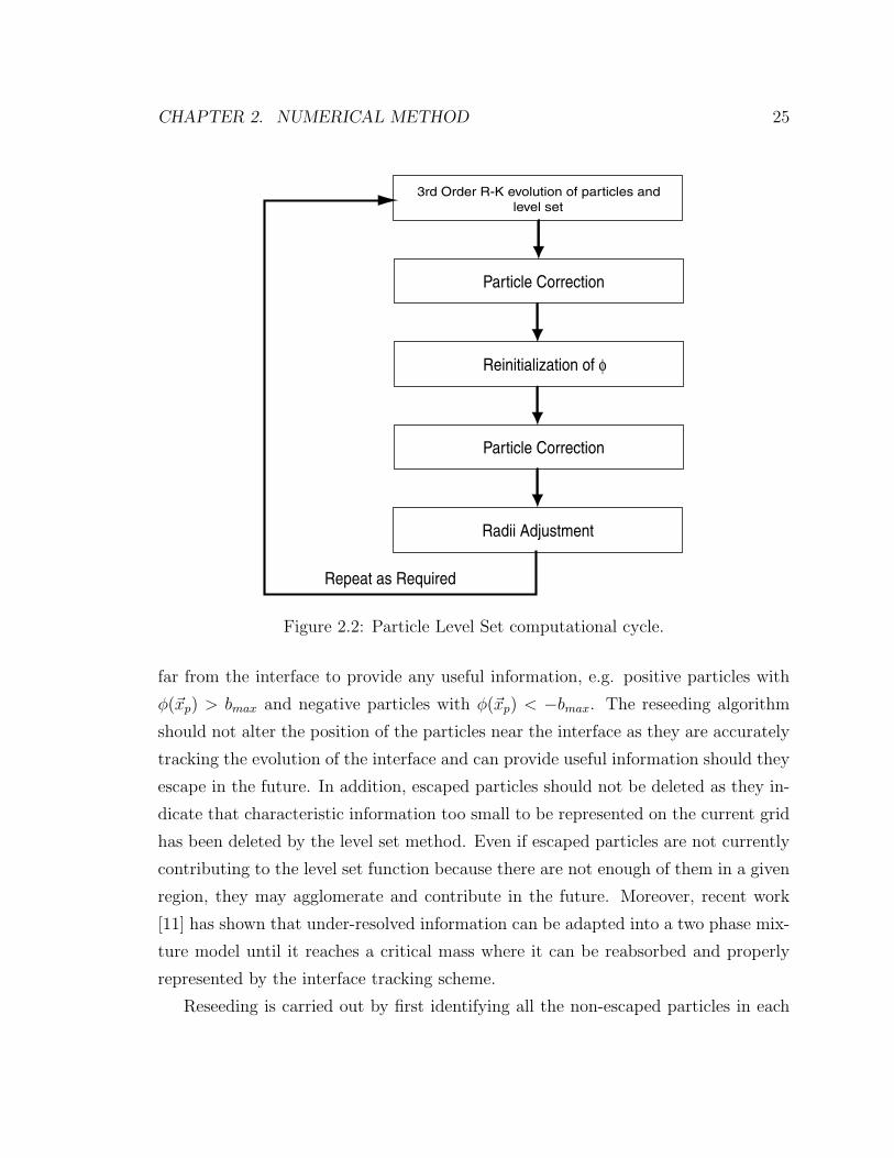
CHAPTER 2. NUMERICAL METHOD 25
3rd Order R-K evolution of particles and level set
Particle Correction
Reinitialization of φ
Particle Correction
Radii Adjustment
Repeat as Required
Figure 2.2: Particle Level Set computational cycle.
far from the interface to provide any useful information, e.g. positive particles with
φ(~xp) > bmax and negative particles with φ(~xp) < −bmax. The reseeding algorithm
should not alter the position of the particles near the interface as they are accurately
tracking the evolution of the interface and can provide useful information should they
escape in the future. In addition, escaped particles should not be deleted as they in-
dicate that characteristic information too small to be represented on the current grid
has been deleted by the level set method. Even if escaped particles are not currently
contributing to the level set function because there are not enough of them in a given
region, they may agglomerate and contribute in the future. Moreover, recent work
[11] has shown that under-resolved information can be adapted into a two phase mix-
ture model until it reaches a critical mass where it can be reabsorbed and properly
represented by the interface tracking scheme.
Reseeding is carried out by first identifying all the non-escaped particles in each
CHAPTER 2. NUMERICAL METHOD 26
cell. Then the local value of the level set function is used to decide if a given cell is
near the interface, e.g. within three grid cells. If a cell is not near the interface, all
the non-escaped particles are deleted. On the other hand, if a cell near the interface
has fewer particles than the previously defined maximum number (e.g. 64 in 3D),
particles are added to the cell and attracted to the interface.
If there are too many non-escaped particles in a given cell, we create a heap data
structure which holds the desired number of particles. Each non-escaped particle
in the cell is inserted into the heap based upon the difference between the locally
interpolated φ(~xp) value and its radius, i.e. spφ(~xp) − rp, since we want to keep the
particles that are closest to the interface. The heap is a computationally and memory
efficient way to store a priority queue. The particle with the largest spφ(~xp) − rp is
placed on top. Once the heap is full and properly sorted, we consider the remaining
particles one at a time. For each remaining particle, its spφ(~xp)−rp value is compared
with the corresponding value of the particle atop the heap. If the current particle
under consideration has a smaller value than the particle atop the heap, we delete
the particle on top of the heap and replace it with the current particle. A down-heap
sort is then performed placing the next candidate for removal atop the heap. If the
current particle’s spφ(~xp)− rp value is larger than that of the particle atop the heap,
we simply delete it.
The reseeding operation is problem dependent. Viable reseeding strategies include
reseeding at fixed time intervals, based upon a measure of the local curvature of the
interface or according to some measure of interface stretching/compression, e.g. arc
length in 2D or surface area in 3D. When reseeding based upon a change in surface
area, level set methods allow easy estimation of this quantity. The surface area of the
interface is given by ∫δ(φ)|∇φ|d~x,
where δ(φ) is a numerically smeared out delta function which to first order accuracy
CHAPTER 2. NUMERICAL METHOD 27
can be approximated as
δ(φ) =
0 φ < −ε12ε
+ 12ε
cos(πφε
) −ε ≤ φ ≤ ε
0 ε < φ,
where ε = 1.5∆x is the bandwidth of the numerical smearing.
Excessive reseeding is not recommended since the inserted particles have to be
attracted to the interface using the current geometry defined by the level set function.
If the interface geometry is poorly resolved, reseeding may not improve the resolution
at the interface. In fact, it may be damaged.
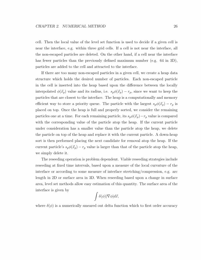
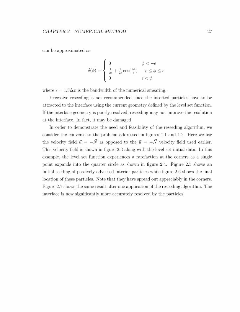
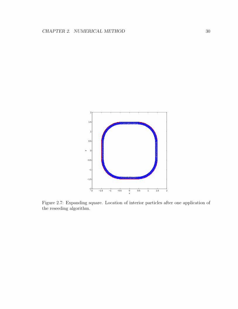
In order to demonstrate the need and feasibility of the reseeding algorithm, we
consider the converse to the problem addressed in figures 1.1 and 1.2. Here we use
the velocity field ~u = − ~N as opposed to the ~u = + ~N velocity field used earlier.
This velocity field is shown in figure 2.3 along with the level set initial data. In this
example, the level set function experiences a rarefaction at the corners as a single
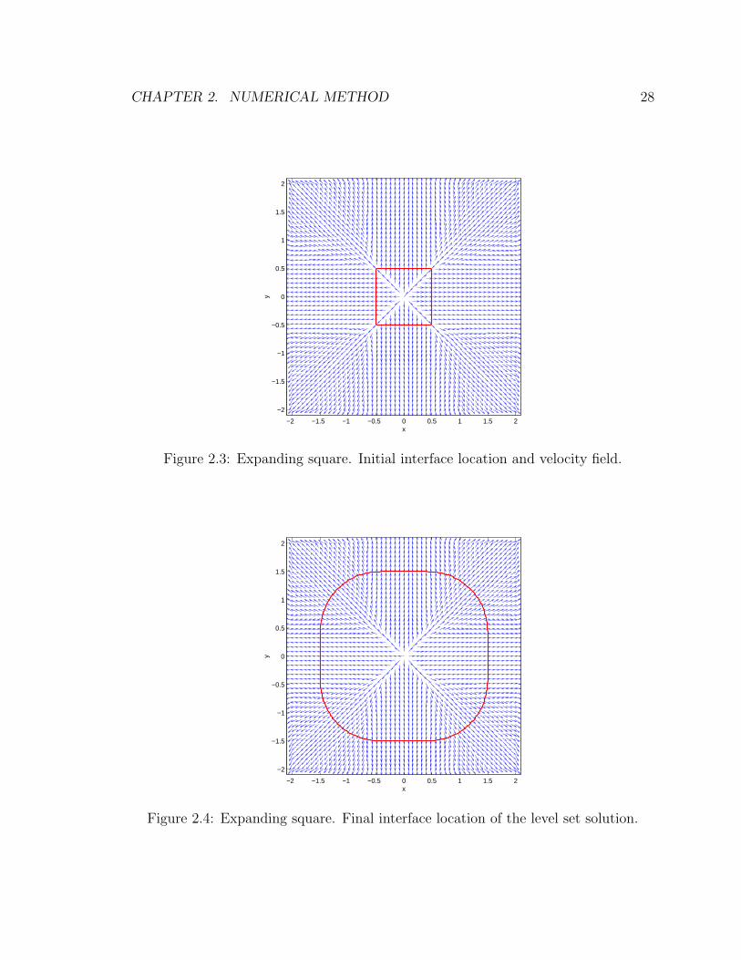
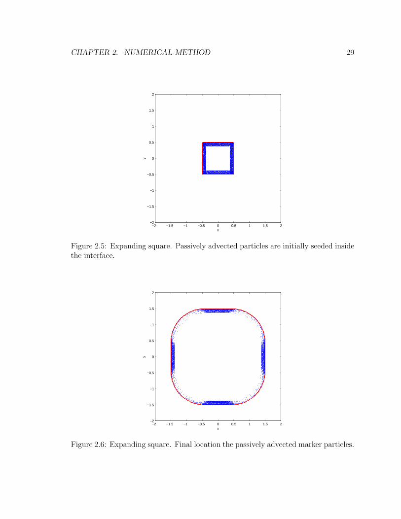
point expands into the quarter circle as shown in figure 2.4. Figure 2.5 shows an
initial seeding of passively advected interior particles while figure 2.6 shows the final
location of these particles. Note that they have spread out appreciably in the corners.
Figure 2.7 shows the same result after one application of the reseeding algorithm. The
interface is now significantly more accurately resolved by the particles.
CHAPTER 2. NUMERICAL METHOD 28
−2 −1.5 −1 −0.5 0 0.5 1 1.5 2
−2
−1.5
−1
−0.5
0
0.5
1
1.5
2
x
y
Figure 2.3: Expanding square. Initial interface location and velocity field.
−2 −1.5 −1 −0.5 0 0.5 1 1.5 2
−2
−1.5
−1
−0.5
0
0.5
1
1.5
2
x
y
Figure 2.4: Expanding square. Final interface location of the level set solution.
CHAPTER 2. NUMERICAL METHOD 29
−2 −1.5 −1 −0.5 0 0.5 1 1.5 2−2
−1.5
−1
−0.5
0
0.5
1
1.5
2
x
y
Figure 2.5: Expanding square. Passively advected particles are initially seeded insidethe interface.
−2 −1.5 −1 −0.5 0 0.5 1 1.5 2−2
−1.5
−1
−0.5
0
0.5
1
1.5
2
x
y
Figure 2.6: Expanding square. Final location the passively advected marker particles.
CHAPTER 2. NUMERICAL METHOD 30
−2 −1.5 −1 −0.5 0 0.5 1 1.5 2−2
−1.5
−1
−0.5
0
0.5
1
1.5
2
x
y
Figure 2.7: Expanding square. Location of interior particles after one application ofthe reseeding algorithm.
Chapter 3
Examples
3.1 Rigid Body Rotation of Zalesak’s Disk
Consider the rigid body rotation of Zalesak’s disk in a solid body velocity field [96].
The initial data is a slotted circle centered at (50,75) with a radius of 15, a width of
5, and a slot length of 25. The velocity field is given by
u = (π/314)(50− y),
v = (π/314)(x− 50),
so that the disk completes one revolution every 628 time units.
Figure 3.1 illustrates the initial seeding of particles on both sides of the interface
while figure 3.2 depicts the particle locations after the attraction step has been applied
to attract them to the appropriate bands on the correct side of the interface. Blue
dots indicate the locations of negative particles and red dots indicate the locations of
positive particles. A 100× 100 grid cell computational mesh is shown in the figures,
showing that the slot is only 5 grid cells across.
Figure 3.3 illustrates the high quality particle level set solution obtained after
one full rotation. Figures 3.4 and 3.5 compare the evolution of a level set only
method (red) and our particle level set method (blue) after one and two revolutions,
respectively. The exact solution (green) is also plotted for the sake of comparison.
31
CHAPTER 3. EXAMPLES 32
As expected, the level set only method applies an excessive amount of regularization
in the sharp corners.
Figure 3.6 illustrates the need for both positive and negative particles. Here, we
plot the level set solution, the particle level set solution and the exact solution along
with both the positive and negative particles. The errors in the level set solution
are emphasized by plotting escaped positive particles in light red and the escaped
negative particles in light blue. This illustrates how the positive particles correct the
errors at the two corners at the top of the slot while the negative particles correct the
errors at the two corners near the bottom of the slot.
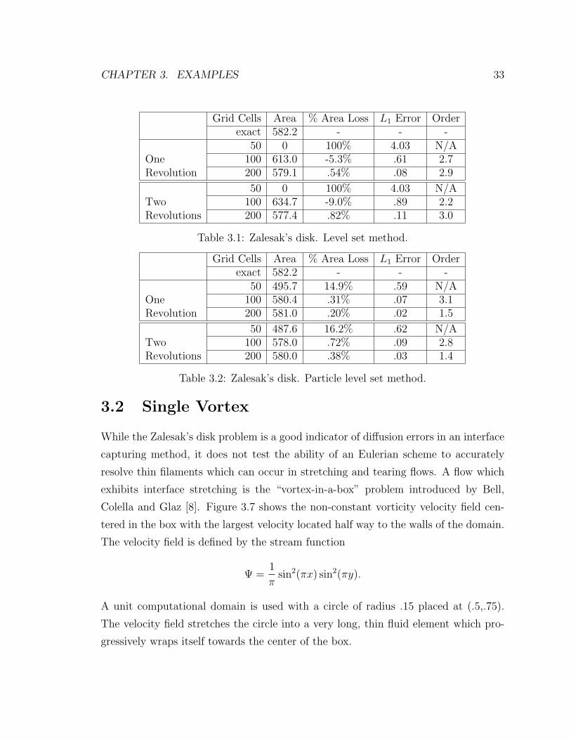
Tables 3.1 and 3.2 compare the area loss (or gain) of the level set method and
the particle level set method on three different grids. The area is calculated using a
second order accurate unbiased level set contouring algorithm [10]. In addition, we
calculate the accuracy of the interface location using the first order accurate error
measure introduced in [83],
1
L
∫|H(φexpected)−H(φcomputed)|dxdy, (3.1)
where L is the length of the expected interface. This integral is numerically calculated
as in [83]:
• partition the domain into many tiny pieces (1000× 1000),
• interpolate φcomputed onto the newly partitioned domain and calculate φexpected
for the domain,
• numerically integrate equation 3.1, where H(φ) is the indicator function for
φ ≤ 0, i.e. H(φ) = 1 if φ ≤ 0 and H(φ) = 0 otherwise.
On the coarsest grid (50 × 50 grid cells), the level set only solution vanishes before
one revolution is completed while the particle level set method still maintains 83.8%
of the area even after two rotations.
CHAPTER 3. EXAMPLES 33
Grid Cells Area % Area Loss L1 Error Orderexact 582.2 - - -
50 0 100% 4.03 N/AOne 100 613.0 -5.3% .61 2.7Revolution 200 579.1 .54% .08 2.9
50 0 100% 4.03 N/ATwo 100 634.7 -9.0% .89 2.2Revolutions 200 577.4 .82% .11 3.0
Table 3.1: Zalesak’s disk. Level set method.
Grid Cells Area % Area Loss L1 Error Orderexact 582.2 - - -
50 495.7 14.9% .59 N/AOne 100 580.4 .31% .07 3.1Revolution 200 581.0 .20% .02 1.5
50 487.6 16.2% .62 N/ATwo 100 578.0 .72% .09 2.8Revolutions 200 580.0 .38% .03 1.4
Table 3.2: Zalesak’s disk. Particle level set method.
3.2 Single Vortex
While the Zalesak’s disk problem is a good indicator of diffusion errors in an interface
capturing method, it does not test the ability of an Eulerian scheme to accurately
resolve thin filaments which can occur in stretching and tearing flows. A flow which
exhibits interface stretching is the “vortex-in-a-box” problem introduced by Bell,
Colella and Glaz [8]. Figure 3.7 shows the non-constant vorticity velocity field cen-
tered in the box with the largest velocity located half way to the walls of the domain.
The velocity field is defined by the stream function
Ψ =1
πsin2(πx) sin2(πy).
A unit computational domain is used with a circle of radius .15 placed at (.5,.75).
The velocity field stretches the circle into a very long, thin fluid element which pro-
gressively wraps itself towards the center of the box.

CHAPTER 3. EXAMPLES 34
Figure 3.8 shows the location of the particles at t = 1 using a 64 × 64 grid. The
positive particles are shown in red while the negative particles are shown in blue.
Even at this relatively early time, there has been a substantial stretching of the
interface, and the particle bands which were initially three grid cells deep have been
stretched and compressed. Both the particle level set solution and a high resolution
front tracked solution are plotted in the figure, although it is difficult to ascertain
which is which as they are almost on top of each other. The role of the particles in
helping to maintain the interface can be seen in figure 3.9 which depicts the level set
solution along with light blue negative particles that have escaped from the level set
solution. Note that escaped particles are found at both the head and tail where the
curvature is large.
The ability of the particle level set method to maintain thin, elongated filaments
is shown in figures 3.10 (at t = 3) and 3.11 (at t = 5). These figures were computed
using 128× 128 grid cells. The interface is depicted in figure 3.10 is at the same time
as in figure 13a in [68] and figures 4a,b,c,d in [67] for the sake of comparison. Both
figures show the level set solution (red), the particle level set solution (blue) and the
high resolution front tracked solution (green). The particle level set method clearly
outperforms the level set method. Only near the head and the tail of the interface
where the level set is about one grid cell wide does the particle level set method fail
to compete with the high resolution front tracked solution. Also note that while the
particle level set method does not conserve area it exhibits less “blobby” structure
than VOF methods, see figure 4d in [67]. In under-resolved regions, the particles are
not close enough together to accurately represent the interface and thin filaments will
break apart. However, the particles still track the interface motion with second order
accuracy so the resulting pieces are in accurate locations. In contrast, the interface
reconstruction procedure used in VOF methods forces mass in neighboring cells to
artificially clump together. As a result, mass in under-resolved regions is moved
inaccurately during the interface reconstruction step, resulting in larger blobs with
first order accurate errors in their location.
For purposes of error analysis, the velocity field is time reversed by allowing the
velocity to have cos(πt/T ) time dependence where T is the time at which the flow

CHAPTER 3. EXAMPLES 35
Grid Cells Area % Area Loss L1 Error Orderexact .0707 - - -
64 0 100.0% .075 N/A128 .0425 39.8% .031 1.3256 .0634 10.3% .008 2.0
Table 3.3: One period of vortex flow. Level set method.
Grid Cells Area % Area Loss L1 Error Orderexact .0707 - - -
64 .0694 1.81% .003 N/A128 .0702 .71% .001 1.1256 .0704 .35% 5.09E-4 1.4
Table 3.4: One period of vortex flow. Particle level set method.
returns to its initial state, see LeVeque [47]. The reversal period used in the error
analysis of the vortex problem is T = 8 producing a maximal stretching of the interface
similar to that shown in figure 3.10. As can be seen from the error tables 3.3 and 3.4
as well as figures 3.12 and 3.13, the ability of the particle level set method to model
interfaces undergoing substantial stretching is quite good. The L1 errors reported
here compare favorably with those reported by Rider and Kothe in [68] using a VOF
PLIC method.
3.3 Deformation Field
An even more difficult test case is the entrainment of a circular body in a deformation
field defined by 16 vortices as introduced by Smolarkiewicz [77]. The periodic velocity
field is given by the stream function
Ψ =1
4πsin(4π(x + .5)) cos(4π(y + .5)). (3.2)
Periodicity is enforced so the portion of the interface that crosses the top boundary
of the domain reappears on the bottom as shown in figure 3.14 at t = 1. The velocity
field given by equation 3.2 is made periodic in time by multiplying the velocity
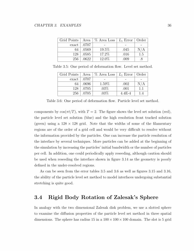
CHAPTER 3. EXAMPLES 36
Grid Points Area % Area Loss L1 Error Orderexact .0707 - - -
64 .0569 19.5% .045 N/A128 .0585 17.2% .016 1.5256 .0622 12.0% .009 .8
Table 3.5: One period of deformation flow. Level set method.
Grid Points Area % Area Loss L1 Error Orderexact .0707 - - -
64 .0696 1.59% .002 N/A128 .0705 .03% .001 1.1256 .0705 .03% 4.4E-4 1.4
Table 3.6: One period of deformation flow. Particle level set method.
components by cos(πt/T ), with T = 2. The figure shows the level set solution (red),
the particle level set solution (blue) and the high resolution front tracked solution
(green) using a 128 × 128 grid. Note that the widths of some of the filamentary
regions are of the order of a grid cell and would be very difficult to resolve without
the information provided by the particles. One can increase the particle resolution of
the interface by several techniques. More particles can be added at the beginning of
the simulation by increasing the particles’ initial bandwidth or the number of particles
per cell. In addition, one could periodically apply reseeding, although caution should
be used when reseeding the interface shown in figure 3.14 as the geometry is poorly
defined in the under-resolved regions.
As can be seen from the error tables 3.5 and 3.6 as well as figures 3.15 and 3.16,
the ability of the particle level set method to model interfaces undergoing substantial
stretching is quite good.
3.4 Rigid Body Rotation of Zalesak’s Sphere
In analogy with the two dimensional Zalesak disk problem, we use a slotted sphere
to examine the diffusion properties of the particle level set method in three spatial
dimensions. The sphere has radius 15 in a 100× 100× 100 domain. The slot is 5 grid
CHAPTER 3. EXAMPLES 37
cells wide and 12.5 grid cells deep on a 100×100×100 grid cell domain. The sphere is
initially placed at (50, 75, 50) and undergoes rigid body rotation in the z = 50 plane
about the point (50, 50, 50). The constant vorticity velocity field is given by
u(x, y, z) = (π/314)(50− y),
v(x, y, z) = (π/314)(x− 50),
w(x, y, z) = 0,
so that the sphere completes one revolution every 628 time units.
The presence of an extra dimension allows for more opportunities to examine an
interface capturing scheme for excessive amounts of regularization. Figures 3.17 and
3.18 show the level set and the particle level set solutions, respectively, at approxi-
mately equally spaced time intervals from t = 0 to t = 628. The final frame at t = 628
should be identical to the initial data at t = 0. The particle level set method is able
to maintain the sharp features of the notch while the level set method is unable to
do so.
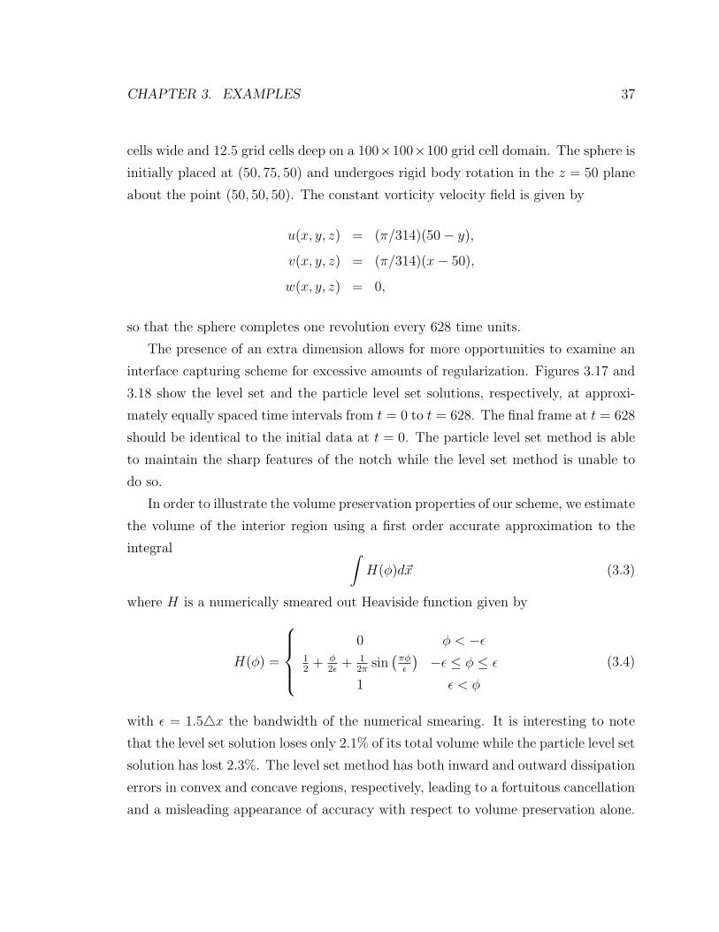
In order to illustrate the volume preservation properties of our scheme, we estimate
the volume of the interior region using a first order accurate approximation to the
integral ∫H(φ)d~x (3.3)
where H is a numerically smeared out Heaviside function given by
H(φ) =
0 φ < −ε12
+ φ2ε
+ 12π
sin(
πφε
) −ε ≤ φ ≤ ε
1 ε < φ
(3.4)
with ε = 1.54x the bandwidth of the numerical smearing. It is interesting to note
that the level set solution loses only 2.1% of its total volume while the particle level set
solution has lost 2.3%. The level set method has both inward and outward dissipation
errors in convex and concave regions, respectively, leading to a fortuitous cancellation
and a misleading appearance of accuracy with respect to volume preservation alone.
CHAPTER 3. EXAMPLES 38
Similar statements hold for VOF calculations that preserve volume almost exactly,
but locate the volume incorrectly, e.g. the creation of spurious flotsam and jetsam.
3.5 Three Dimensional Deformation Field
LeVeque [47] proposed a three dimensional incompressible flow field which combines
a deformation in the x-y plane with one in the x-z plane. The velocity field is given
by
u(x, y, z) = 2 sin2(πx) sin(2πy) sin(2πz),
v(x, y, z) = − sin(2πx) sin2(πy) sin(2πz),
w(x, y, z) = − sin(2πx) sin(2πy) sin2(πz)
and the flow field is modulated in time with a period of T = 3. A sphere of radius .15
is placed within a unit computational domain at (.35, .35, .35). A 100×100×100 grid
cell domain was used. This allows the sphere to be entrained by two rotating vortices
which initially scoop out opposite sides of the sphere and then compress them causing
the sphere to pancake. The top and bottom edges of the pancake are then caught
up again in the vortices causing the surface to become very stretched. Parts of the
interface thin out to about a grid cell and both methods have difficulty resolving this
thin interface. Of course, we could use a variety of techniques to increase the initial
particle density or to reseed along the way, but the particle level set method recovers
rather nicely and loses very little volume even without increasing the particle count.
On the other hand, the level set method fails severely in this example.
Figures 3.19 and 3.20 show the level set solution and the particle level set solution,
respectively, at t = 0, 104s, 204s, 304s, 404s, 504s, 604s, 704s, 904s, 1104s,
1304s and 1504s where 4s = 628/150. The final frame at t = 1504s should be
identical to the initial data at t = 0. In addition, frame 1304s should be identical to
frame 204s, frame 1104s should be identical to frame 404s, and frame 904s should
be identical to frame 604s. The maximum stretching occurs at t = 754s where the
level set solution has lost 49% of the initial volume and the particle level set solution
CHAPTER 3. EXAMPLES 39
has gained 1.9%. After completing a full cycle, at t = 1504s, the level set solution
has lost 80% of the initial volume while the particle level set solution has only lost
2.6%.
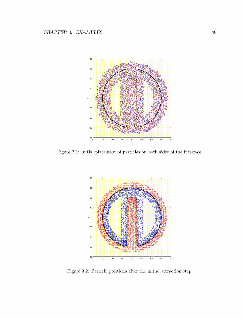
CHAPTER 3. EXAMPLES 40
30 35 40 45 50 55 60 65 7055
60
65
70
75
80
85
90
95
x
y
Figure 3.1: Initial placement of particles on both sides of the interface.
30 35 40 45 50 55 60 65 7055
60
65
70
75
80
85
90
95
x
y
Figure 3.2: Particle positions after the initial attraction step.

CHAPTER 3. EXAMPLES 41
30 35 40 45 50 55 60 65 7055
60
65
70
75
80
85
90
95
x
y
Figure 3.3: Particle level set solution after one revolution.
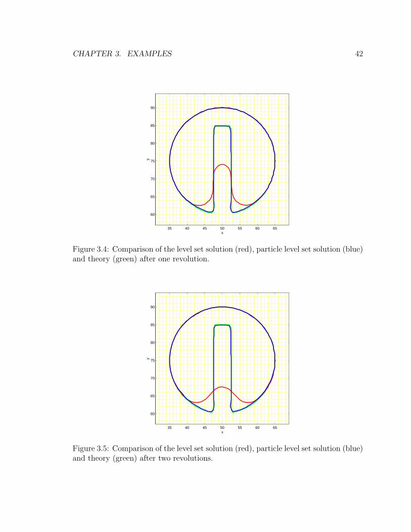
CHAPTER 3. EXAMPLES 42
35 40 45 50 55 60 65
60
65
70
75
80
85
90
x
y
Figure 3.4: Comparison of the level set solution (red), particle level set solution (blue)and theory (green) after one revolution.
35 40 45 50 55 60 65
60
65
70
75
80
85
90
x
y
Figure 3.5: Comparison of the level set solution (red), particle level set solution (blue)and theory (green) after two revolutions.

CHAPTER 3. EXAMPLES 43
30 35 40 45 50 55 60 65 7055
60
65
70
75
80
85
90
95
x
y
Figure 3.6: Comparison of the level set solution, particle level set solution and theoryafter one revolution. The light red particles and light blue particles have escapedfrom the level set solution.

CHAPTER 3. EXAMPLES 44
0 0.1 0.2 0.3 0.4 0.5 0.6 0.7 0.8 0.9 10
0.1
0.2
0.3
0.4
0.5
0.6
0.7
0.8
0.9
1
x
y
Figure 3.7: Initial data and velocity field for the vortex flow.
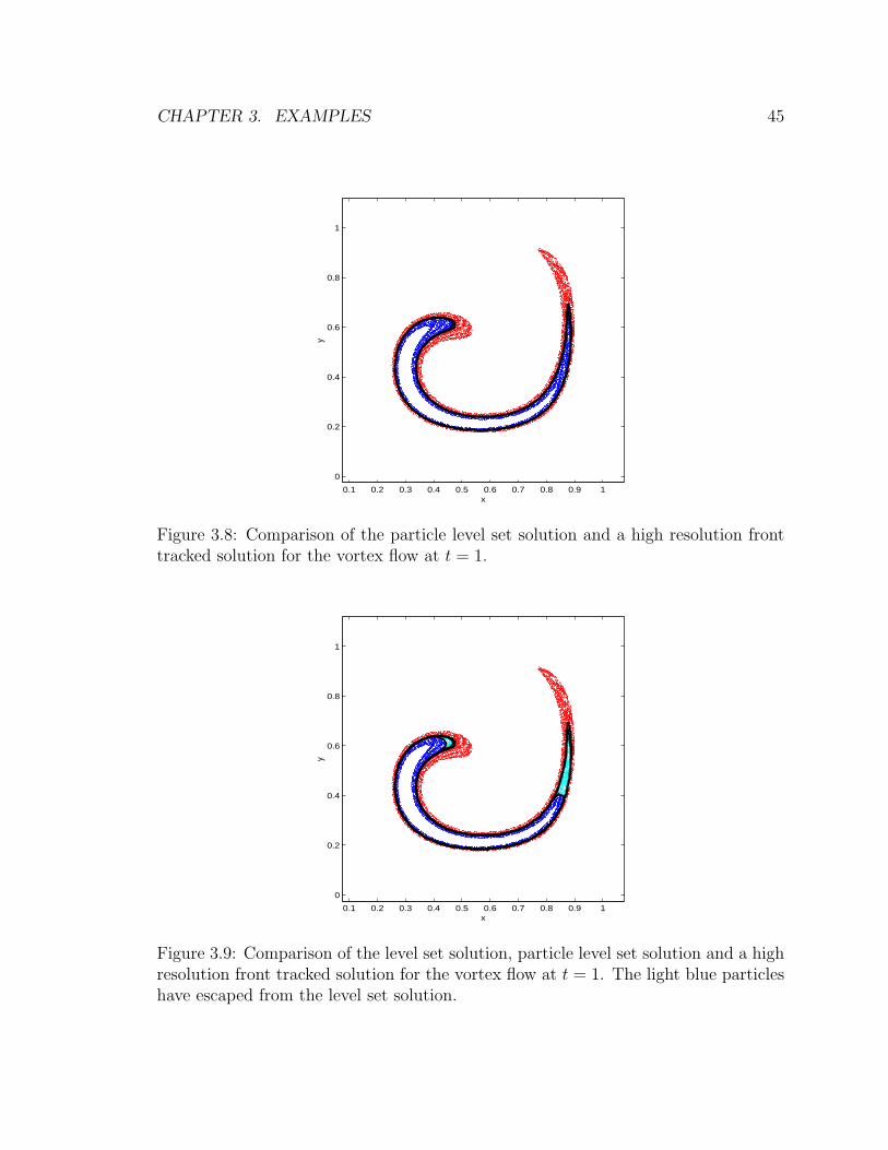
CHAPTER 3. EXAMPLES 45
0.1 0.2 0.3 0.4 0.5 0.6 0.7 0.8 0.9 1
0
0.2
0.4
0.6
0.8
1
x
y
Figure 3.8: Comparison of the particle level set solution and a high resolution fronttracked solution for the vortex flow at t = 1.
0.1 0.2 0.3 0.4 0.5 0.6 0.7 0.8 0.9 1
0
0.2
0.4
0.6
0.8
1
x
y
Figure 3.9: Comparison of the level set solution, particle level set solution and a highresolution front tracked solution for the vortex flow at t = 1. The light blue particleshave escaped from the level set solution.
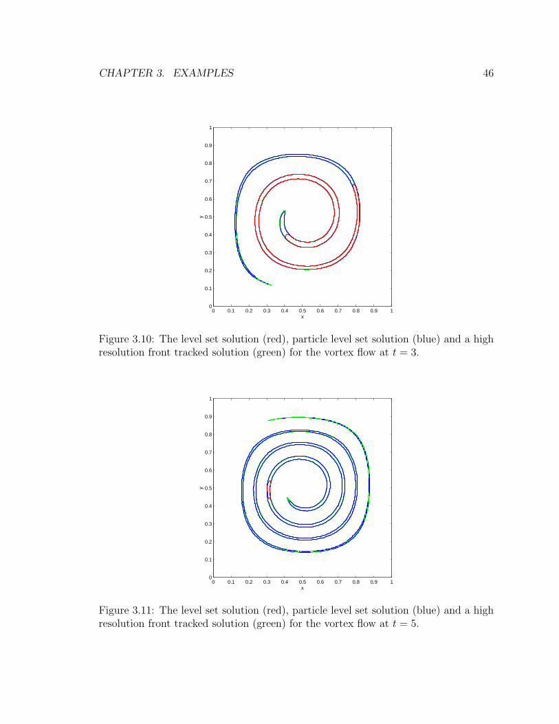
CHAPTER 3. EXAMPLES 46
0 0.1 0.2 0.3 0.4 0.5 0.6 0.7 0.8 0.9 10
0.1
0.2
0.3
0.4
0.5
0.6
0.7
0.8
0.9
1
x
y
Figure 3.10: The level set solution (red), particle level set solution (blue) and a highresolution front tracked solution (green) for the vortex flow at t = 3.
0 0.1 0.2 0.3 0.4 0.5 0.6 0.7 0.8 0.9 10
0.1
0.2
0.3
0.4
0.5
0.6
0.7
0.8
0.9
1
x
y
Figure 3.11: The level set solution (red), particle level set solution (blue) and a highresolution front tracked solution (green) for the vortex flow at t = 5.
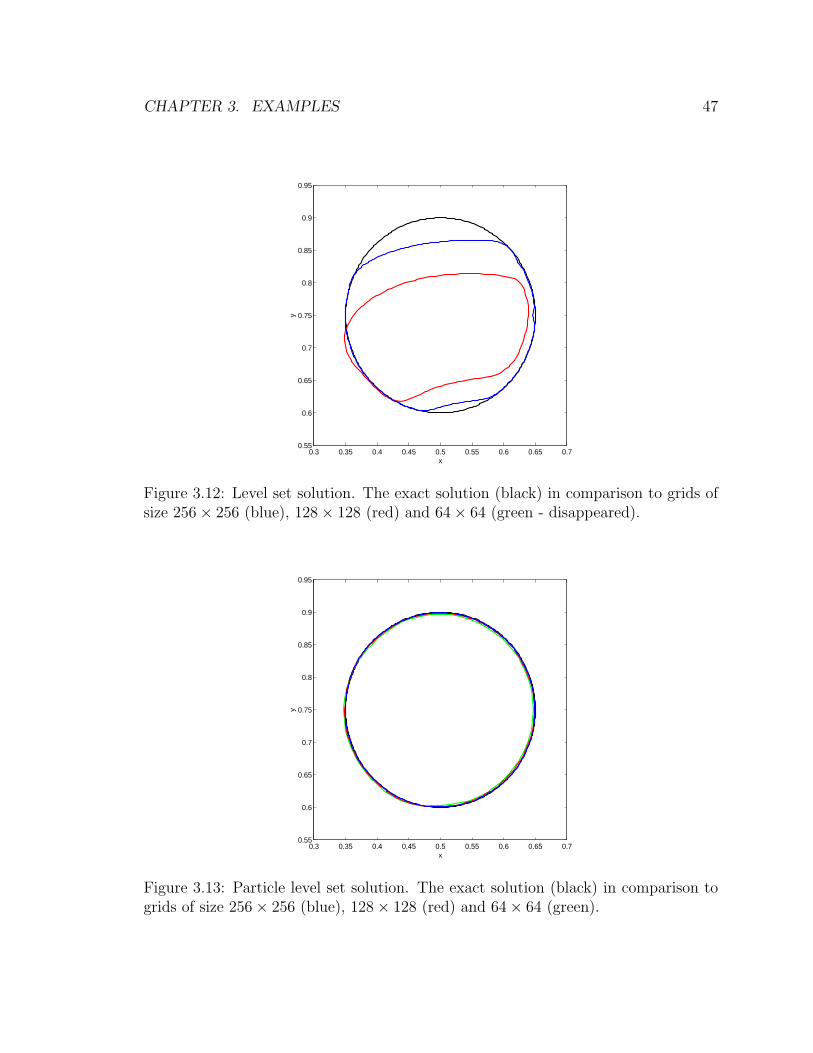
CHAPTER 3. EXAMPLES 47
0.3 0.35 0.4 0.45 0.5 0.55 0.6 0.65 0.70.55
0.6
0.65
0.7
0.75
0.8
0.85
0.9
0.95
x
y
Figure 3.12: Level set solution. The exact solution (black) in comparison to grids ofsize 256× 256 (blue), 128× 128 (red) and 64× 64 (green - disappeared).
0.3 0.35 0.4 0.45 0.5 0.55 0.6 0.65 0.70.55
0.6
0.65
0.7
0.75
0.8
0.85
0.9
0.95
x
y
Figure 3.13: Particle level set solution. The exact solution (black) in comparison togrids of size 256× 256 (blue), 128× 128 (red) and 64× 64 (green).

CHAPTER 3. EXAMPLES 48
0 0.1 0.2 0.3 0.4 0.5 0.6 0.7 0.8 0.9 10
0.1
0.2
0.3
0.4
0.5
0.6
0.7
0.8
0.9
1
x
y
Figure 3.14: Comparison of the level set solution (red), particle level set solution(blue) and a high resolution front tracked solution (green) for the deformation flowat t = 1.
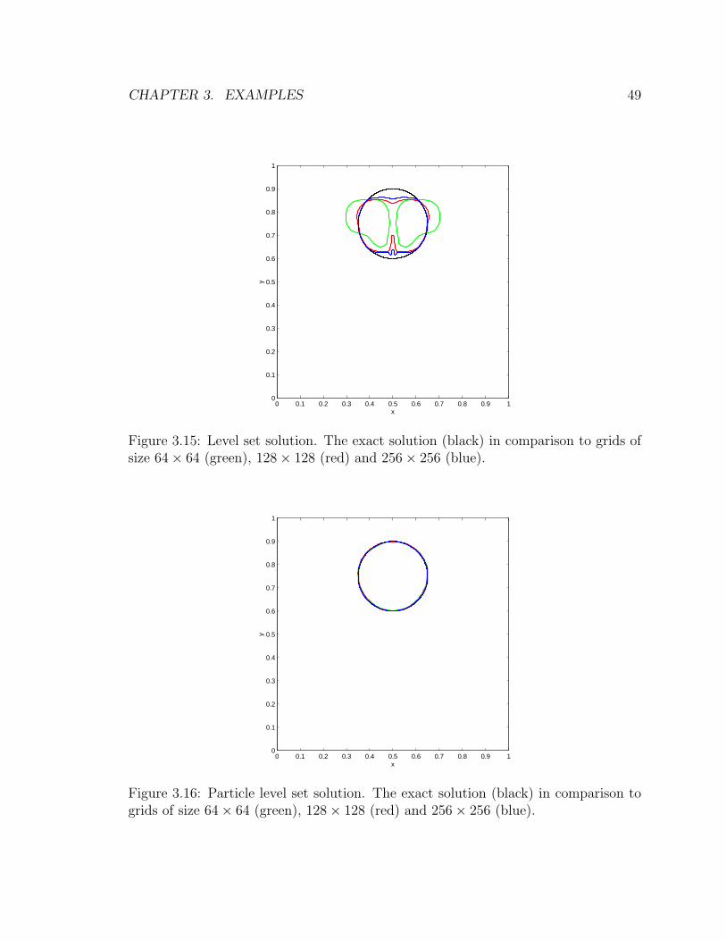
CHAPTER 3. EXAMPLES 49
0 0.1 0.2 0.3 0.4 0.5 0.6 0.7 0.8 0.9 10
0.1
0.2
0.3
0.4
0.5
0.6
0.7
0.8
0.9
1
x
y
Figure 3.15: Level set solution. The exact solution (black) in comparison to grids ofsize 64× 64 (green), 128× 128 (red) and 256× 256 (blue).
0 0.1 0.2 0.3 0.4 0.5 0.6 0.7 0.8 0.9 10
0.1
0.2
0.3
0.4
0.5
0.6
0.7
0.8
0.9
1
x
y
Figure 3.16: Particle level set solution. The exact solution (black) in comparison togrids of size 64× 64 (green), 128× 128 (red) and 256× 256 (blue).

CHAPTER 3. EXAMPLES 50
Figure 3.17: Zalesak’s sphere. Level set solution.
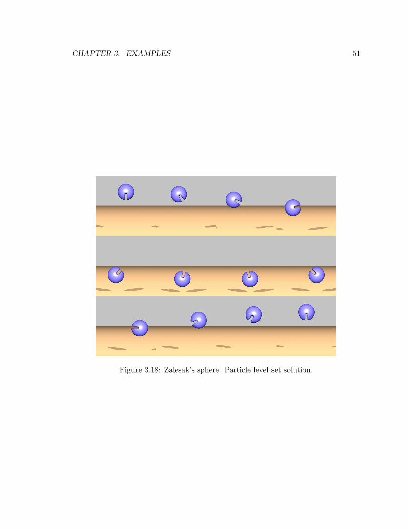
CHAPTER 3. EXAMPLES 51
Figure 3.18: Zalesak’s sphere. Particle level set solution.

CHAPTER 3. EXAMPLES 52
Figure 3.19: Deformation test case. Level set solution.
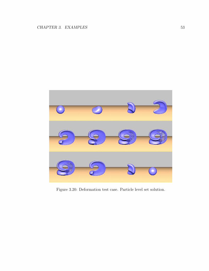
CHAPTER 3. EXAMPLES 53
Figure 3.20: Deformation test case. Particle level set solution.
Chapter 4
Free Surface Calculations
“In the time honored tradition of computer graphics,we can now go ahead and steal anything we can get.”
Fournier and Reeves [26]
4.1 Liquid Free Surface Flows
The ubiquity of water in our everyday lives has motivated scientists and engineers
to attempt to simulate a wide variety of liquid phenomena. The simulation of the
destructive force of tsunamis and waves on beaches [48, 40, 29]; the breakup of thin
sheets of liquid fuel [49, 43] or the formation of ink drops for printing [4]; the filling of
containers for food industry applications [88, 87]; and the adhesion of two circulatory
cells under shear flow [3], has prompted the development of a wide variety of novel
methods to describe the motion of the liquid and the free surface present in each of
these applications. A common theme among all of these applications is the complex,
three-dimensional behavior of the interface. Any method used to describe the behav-
ior of the free surface needs to be capable of capturing these aspects of water surfaces.
Besides the obvious economic and environmental importance of being able to develop
mechanisms to control the liquid through improved numerical modeling, the lively,
complex motion of the free surface is often visually attractive to the casual observer.
This attractiveness has recently motivated the computer graphics community to take
54
CHAPTER 4. FREE SURFACE CALCULATIONS 55
an interest in the realistic animation of complex water surfaces.
4.2 CFD and Computer Animation
The use of computational fluid dynamics to mimic liquid behavior for purposes of
computer animation is a relatively recent phenomenon. While the engineering and
scientific communities wish to achieve the highest fidelity possible in a simulation,
the animation community does not need to achieve this goal. Rather, the goal is to
achieve a “believable” liquid performance. This liberates the animator from being
forced to use a realistic model of a liquid. While the animator has a lot of freedom
as to how to animate a liquid, liquids are governed by certain physical laws so it
makes sense that an animator will utilize simplifying assumptions in order to obtain
the desired performance. This approach to the animation of liquids has been used
extensively by the animation community. Original efforts to obtain two dimensional
wave behavior is seen in the efforts of Masten [51] using Fourier synthesis techniques
and Schachter [69] with a parametric representation of the water surface. Peachey [61]
borrowed features of Airy models and Fournier and Reeves [26] utilized Gerstner wave
theory to generate realistic looking periodic waves which appear to almost break.
To obtain more realistic liquid performances, the animation community then
turned towards two dimensional approximations to the full three dimensional Navier-
Stokes equations. A height field representation of the water surface used by Kass
and Miller [42] was derived from a linearized form of the two dimensional shallow
water equations. Interaction with obstacles using a pressure determined height field
formulation was used by Chen and Lobo [14]. Two dimensional splashing liquids with
spray being modeled by particles was presented in [57]. As an alternative to Navier-
Stokes models, a viscous spring-particle representation of a liquid has been proposed
by Miller and Pearce [53] and a molecular dynamics approach was used in [86].
While the above approaches have been and continue to be used in the animation
community, exciting and dynamic water behavior can only result from the use of fully
three dimensional computational fluid dynamics algorithms. Foster and Metaxas [25]
CHAPTER 4. FREE SURFACE CALCULATIONS 56
built upon the original CFD work of Harlow and Welch [31] in creating a 3D Navier-
Stokes methodology for the realistic animation of liquids. A staggered flow grid
arrangement was used along with a marker particle representation of the liquid. Both
the convective and viscous terms were discretized using central differencing and the
entire system was integrated in time using a forward Euler scheme. In the case of
animating water or other relatively inviscid substances, the combination of spatial
central differencing for the convective terms and a forward Euler time discretization
can pose a severe time step restriction, i.e. ∆t ∼ (∆x)2, for the simulation to remain
stable. Even if upwind differencing is used for the convection terms, a CFL condition
of u∆t/∆x < 1 will need to be obeyed. Stam in 1999 [78] proposed a “Stable Fluid”
approach to the treatment of the convective term in the Navier-Stokes equations for
animation applications. This “Stable Fluid” approach is really a semi-Lagrangian
method first proposed in 1952 by Courant, Issacson, and Rees [20]. Besides its pro-
posed use in the animation community, semi-Lagrangian methods are popular in the
meteorological community for their stability characteristics [52, 79]. Use of a semi-
Lagrangian method allows a liquid animation to remain stable even when using time
steps larger than that given by a traditional CFL condition for Eulerian finite differ-
ence schemes, providing tremendous computational savings by reducing the number
pressure calculations done at the cost of introducing additional amounts of numerical
viscosity.
While the seminal work of Foster and Metaxas introduced the use of fully three
dimensional Navier-Stokes simulations for the purposes of animating liquids, the prac-
tical application of CFD technology for liquid animations was introduced by Foster
and Fedkiw [24]. Some of these contributions include:
• A semi-Lagrangian “Stable Fluid” approach for the convective terms in order
to minimize number of expensive pressure iterations;
• Use of a novel hybrid liquid volume model combining a level set and marker
particle approach to represent the liquid;
• Time step subcycling for the evolution of particles and level set in order to
maintain stability of the interface given CFL violating large liquid time steps;
CHAPTER 4. FREE SURFACE CALCULATIONS 57
• Use of an efficient Preconditioned Conjugate Gradient method to solve for the
pressure during the projection step, unlike the slow SOR method used by Foster
and Metaxas;
• Formulation of plausible velocity boundary conditions for moving objects in the
liquid.
The combination of all of these technologies has begun to meet the engineering re-
quirements for the use of fully three dimensional computational fluid dynamics al-
gorithms in a computer animation environment. Utilization of inherently stable al-
gorithms to avoid having animators not trained in computational methods perform
costly numerical stability studies; use of fast numerical algorithms for quick turn
around time; robust and accurate interface methods used to convey the presence of
the free surface even on the coarse grids commonly used by animators; and interactive
algorithms which allows for the possibility of controlling the behavior of the liquid
and the ability for the liquid to affect the motion of objects and vice versa.
We wish to focus for a moment on the hybrid volume model utilized by Foster and
Fedkiw to model the free surface of the liquid. The use of a level set only representa-
tion for the interface introduces difficulties in maintaining the liquid volume on the
coarse grids commonly used in an animation environment as discussed in Chapter 2.
This difficulty was recognized by Foster and Fedkiw and marker particles were used
to represent the volume of liquid in regions of high curvature near the interface. To
illustrate the behavior of the hybrid volume model, the resulting interface after one
rotation of Zalesak’s disk is shown in figure 4.1(c). The Foster and Fedkiw scheme
does an excellent job of preserving the liquid volume as compared to a level set only
method, but it is at the expense of not preserving the air in the notch. The problem
with the hybrid volume model is that it does not model the opposite side of the in-
terface, the air side of the interface in this case. The particle level set result on the
other hand as seen in figure 4.1(d) does not favor one side of the interface over the
other and is able to maintain the sharpness of the notch.
While CFD algorithms have been slowly working their way into a traditional pro-
duction animation environment [95], the combination of all of the above technologies

CHAPTER 4. FREE SURFACE CALCULATIONS 58
has made it feasible to perform fully three dimensional simulations for animating
liquids.
4.3 Liquid Model
4.3.1 Navier-Stokes Equations
Our simulations utilize the three dimensional Navier-Stokes equations given by
~ut = −~u · ∇~u + ν∇ · (∇~u)− 1
ρ∇p + ~g, (4.1)
where ~u = (u, v, w) is the velocity, ν is the kinematic viscosity of the liquid, ρ is
the density of the liquid, p is the pressure, and ~g is an externally applied gravity
field. While nothing in our computational scheme precludes the simulation of highly
viscous flows, the viscosity of water is negligible so we do not explicitly model the
second term on the right hand side of equation 4.1. In order to calculate the pressure
we impose the incompressibility constraint on the liquid resulting from the law of
conservation of mass,
∇ · ~u = 0. (4.2)
At a wall, we choose to apply a flow tangency boundary condition. If we define
~N to be the normal to the wall and ~T1 and ~T2 to be two mutually orthogonal tangent
vectors to the wall, we impose
~u · ~N = 0 (4.3)
∇~u · ~T1 = ∇~u · ~T2 = 0. (4.4)
By performing the simulation using a staggered velocity-pressure (MAC grid) ar-
rangement we can avoid specifying a pressure boundary condition at the wall. The
velocity and pressure boundary conditions at the free surface are discussed below.
The boundary conditions we impose in the presence of objects placed in the liquid
are discussed in section 4.5.3.

CHAPTER 4. FREE SURFACE CALCULATIONS 59
Finally, we usually begin the simulation with a specified velocity field and an
initial position for the free surface.
4.3.2 Free Surface Boundary Conditions
We do not solve equations 4.1 and 4.2 over the entire computational domain, but only
in the regions occupied by the liquid. Our calculations do not model the dynamics
of the air on the free surface as in a truly multiphase calculation. In general, two
boundary conditions apply at the free surface:
• The kinematic condition states that there is no transport of mass through the
interface. Mathematically we can represent this condition as
[~u− ~ufs]fs · ~N = 0, (4.5)
where ~ufs is the velocity of the free surface and the jump condition is taken
at the boundary. Practically, this means that the level set should take as its
velocity field that of the fluid and the marker particles should interpolate their
velocity from the fluid velocity.
• The dynamic condition is a statement of momentum conservation at the free
surface, i.e. the fluid forces at the free surface are in equilibrium. In general,
the presence of surface tension causes a jump in the normal stress while the
tangential stresses are continuous across the interface,
[σijnj]fs = τκni (4.6a)
[σijtj]fs = 0 (4.6b)
[σijsj]fs = 0, (4.6c)
where
σij = −pδij + ν(ui,j + uj,i), (4.7)
nj is the normal to the interface, tj and sj are mutually orthogonal tangents
to the interface, τ is the coefficient of surface tension and κ is the curvature.
CHAPTER 4. FREE SURFACE CALCULATIONS 60
A way to explicitly capture discrete jump conditions at the interface using
level set technology is by the “Ghost Fluid” method of Fedkiw and collabo-
rators [23, 41, 55]. In our case since we are not explicitly modeling one side
of the interface, we do not need to use such methods. We neglect the shear
stress conditions, eqns. 4.6b and 4.6c. Also, we neglect surface tension effects,
reducing equation 4.6a to a statement that the pressure across the interface is
continuous, i.e. pliquid = pair. In the examples presented in this dissertation,
pair is set to 0.
4.4 Computational Method
In this work we utilize the methodology described in [24] to solve for the velocity and
pressure at each time step. In addition, the particle level set method is used to model
the interface.
4.4.1 Finite Difference Discretization
A staggered MAC grid arrangement [31] is used to represent the velocity and pressure
on a Cartesian computational grid. The pressure is stored at cell centers, while
the components of the velocity are stored on the appropriate cell face as illustrated
in figure 4.2. On a domain of size (xmin, xmax) × (ymin, ymax) × (zmin, zmax) with
(1,m) × (1, n) × (1, mn) grid points, ∆x is given by (xmax − xmin)/m and ~xi,j,k =
(xmin + (i− .5) ∆x, ymin + (j − .5) ∆y, zmin + (k − .5) ∆z).
An explicit first order in time fractional step method [44] utilizing the velocity
projection method of Chorin [18] is used to advance the velocity and pressure fields
in time. The convective term is discretized using a “Stable Fluid” semi-Lagrangian
approach. An intermediate velocity field, ~u∗ is calculated by
u∗i+1/2,j,k = un(~xi+1/2,j,k − ~uni+1/2,j,k ∆t) (4.8a)
v∗i,j+1/2,k = vn(~xi,j+1/2,k − ~uni,j+1/2,k ∆t)− g∆t (4.8b)
w∗i,j,k+1/2 = wn(~xi,j,k+1/2 − ~un
i,j,k+1/2 ∆t), (4.8c)

CHAPTER 4. FREE SURFACE CALCULATIONS 61
where g is the gravitational constant, 9.8m/s2. Trilinear interpolation is used to
obtain values of the components of ~u which do not lie on grid points.
The new liquid velocity ~un+1 is defined by
un+1i+1/2,j,k − u∗i+1/2,j,k
∆t+
pn+1/2i+1,j,k − p
n+1/2i,j,k
ρ= 0 (4.9a)
vn+1i,j+1/2,k − v∗i,j+1/2,k
∆t+
pn+1/2i,j+1,k − p
n+1/2i,j,k
ρ= 0 (4.9b)
wn+1i,j,k+1/2 − w∗
i,j,k+1/2
∆t+
pn+1/2i,j,k+1 − p
n+1/2i,j,k
ρ= 0. (4.9c)
Imposing the incompressibility constraint of equation 4.2 on ~un+1, results in
∇ · ~u∗∆t
= ∇ ·(∇pn+1/2
ρ
). (4.10)
Written in component form, we obtain the following equation for pi,j,k at the n + 1/2
time level,
pi+1,j,k + pi,j+1,k + pi,j,k+1 − 6pi,j,k + pi−1,j,k + pi,j−1,k + pi,j,k−1 = ρ∆x
∆tDi,j,k (4.11)
assuming ∆x = ∆y = ∆z. Di,j,k is the numerical divergence of the velocity defined
as
Di,j,k = u∗i+1/2,j,k − u∗i−1/2,j,k + v∗i,j+1/2,k − v∗i,j−1/2,k + w∗i,j,k+1/2 − w∗
i,j,k−1/2. (4.12)
From equation 4.11 we can calculate the pressure, pn+1/2, needed to ensure that
the velocity is divergence-free at the n + 1 time level. Since the system described
by 4.11 is symmetric and positive definite (as long as there is at least one surface cell
in the computational domain which slightly modifies the system as discussed below),
we use an efficient Preconditioned Conjugate Gradient (PCG) as discussed in Golub
and VanLoan [28] to determine pn+1/2i,j,k .
CHAPTER 4. FREE SURFACE CALCULATIONS 62
4.4.2 Velocity Extrapolation Near Free Surface
The presence of the free surface introduces some additional computational issues,
especially in the treatment of equations 4.11 and 4.12. Due to our modeling assump-
tions, we apply the results of the above calculations only in cells which contain liquid.
Cells with φi,j,k ≤ 0 at the center are determined to contain liquid. Surface cells are
those which contain the φ = 0 isocontour. In cells which have φi,j,k > 0, we impose a
Dirichlet boundary condition and define the pressure to be 0. This condition modifies
the left-hand side of equation 4.11 by setting to zero any off-diagonal pressure terms
in cells which have φi±1,j±1,k±1 > 0. The diagonal term is set to the number of neigh-
boring liquid cells. The imposition of this boundary condition at cell centers and not
at the exact location of the free surface introduces some error into the simulation,
consequently degrading the calculation to first order accuracy near the interface. The
accumulation of this error over time can degrade the accuracy of a simulation. In
order to apply the pressure condition at the actual location of the free surface, an
irregular finite difference stencil can be used as discussed in [12]. However, use of this
more complicated stencil for the purposes of animation appears to be unnecessary as
the results presented later in this chapter indicate.
A variety of methods have been used to computationally treat the calculation
of the divergence of the velocity field on the interface. Velocities on the faces of
surface cells which are adjacent to non-liquid cells will need to be determined even
though these velocities may not lie within the liquid and are not explicitly modeled.
A commonly used condition [31, 6, 25] is to set the undetermined velocities so that
Di,j,k = 0 is satisfied. Unfortunately, there are 64 distinct velocity configurations
which need to be accounted for in three dimensions, not including the possibilities
resulting from the presence of objects in the liquid or of walls at the boundaries.
A less than rigorous analysis of all the possibilities can lead to the introduction of
non-physical asymmetries into a simulation. For example, a detailed analysis of the
computational velocity boundary conditions resulting from enforcing Di,j,k = 0 at
the free surface [15] showed that the velocity boundary conditions in the popular
SMAC method [6] contained such an asymmetry. On the other hand Chan and
Street [12] did not enforce Di,j,k = 0 at the free surface since the free surface boundary

CHAPTER 4. FREE SURFACE CALCULATIONS 63
conditions discussed in section 4.3.2 do not place any conditions on Di,j,k. Rather,
they extrapolated the velocities from the liquid into the air using a Gregory-Newton
backward interpolation formula in order to obtain a higher order accurate calculation
of the velocity of the free surface. Even in highly viscous flows, faithful adherence of
the simulation to the stress-free boundary conditions, eqns. 4.6a, 4.6b, and 4.6c is
important in order to obtain physically accurate results [35, 56].
We choose to take a new approach to setting the unmodeled, but computationally
required velocities, that takes advantage of the geometrical information contained in
the level set function used to describe the free surface. We smoothly extrapolate
the fluid velocities in the normal direction to the interface from inside the liquid.
While this technique of extrapolating the velocity of the interface smoothly over the
entire domain was first introduced to the level set community by Adalsteinsson and
Sethian [2], its application to a free surface calculation is new. To calculate the
extrapolated velocity, ~uext = (uext, vext, wext), away from the interface we solve to
steady state
∂uext
∂τ+ ~N · ∇uext = 0 (4.13a)
∂vext
∂τ+ ~N · ∇vext = 0 (4.13b)
∂wext
∂τ+ ~N · ∇wext = 0, (4.13c)
where τ is a fictitious time. The above equations are solved in band of 5 grid cells
thick near the interface where φ > 0. Since we have signed distance information to the
free surface for the entire computational domain, ~N is given by ∇φ. At steady state
we note that ∇φ · ∇uext, vext, wext = 0. This condition satisfies Di,j,k = 0 at the
free surface in the limit as the grid spacing approaches zero, since the divergence-free
velocities are propagated unchanged in the normal direction across the interface. Also,
since the update of the extrapolated variables occurs in only one direction outward
from the interface, a fast O(n log n) marching technique [1] can be used to update
~uext.
CHAPTER 4. FREE SURFACE CALCULATIONS 64
Use of this velocity extrapolation technique allows us to obtain a physically plau-
sible velocity field in regions where we do not explicitly model the liquid. Besides
providing for a reasonable way to calculate Di,j,k at the free surface, we can utilize the
extrapolated velocity field for other purposes. Since we are using the particle level
set method to model the interface, the existence of particles in the unmodeled “air”
side of the interface requires that we have a reasonable velocity field in this region
in order to move the particles. These particles are typically in a band a couple of
grid cells thick about the interface, so having the capability to smoothly extrapolate
velocities more than one grid cell away from the interface is crucial. Also, when us-
ing a semi-Lagrangian technique to update the velocity field inside the liquid near
the interface, the flow characteristics may look back into the φ > 0 region near the
interface in order to determine which velocities to use in the update.
4.4.3 Particle Level Set Interface Treatment
We utilize the particle level set method as described in chapter 2 to model the inter-
face. A dimension by dimension discretization of
φt + ~u · ∇φ = 0 (4.14)
using a fifth order accurate H-J WENO scheme is used along with a first order accurate
forward Euler update in time. The particles are updated in time with a first order
accurate forward Euler method which uses the velocities at time level n, i.e.
~xn+1p = ~xn
p + ~un(~xnp ). (4.15)
Trilinear interpolation is used to determine the velocity of each particle.
For the examples shown in section 4.5 we perform a particle reseeding step every
20 frames. This reseeding is performed in order to maintain a reasonable distribution
of particles about the entire fluid interface. This is necessary for the error correction
step of the particle level set method to be effective. 64 particles per cell are used at
all reseeding steps.

CHAPTER 4. FREE SURFACE CALCULATIONS 65
4.4.4 Boundaries
All of our calculations are performed in a computational domain which is open on the
air at the top (j = n). We maintain a 3 grid cell thick band of ghost cells around the
computational domain to assist in the semi-Lagrangian update of the velocity near
the boundaries. For the level set we reflect the value of φ across the front, back, left,
right, and bottom boundaries,
φ1−l,j,k = φl,j,k, φm+l,j,k = φm−(l−1),j,k, (4.16a)
φi,j,1−l = φi,j,l, φi,j,mn+l = φi,j,mn−(l−1), (4.16b)
φi,1−l,k = φi,l,k, (4.16c)
where l = 1, 2, 3, i ∈ (1,m), j ∈ (1, n), k ∈ (1,mn). We wish to ensure that “air”
or φ > 0 is always above the computational domain at the j = n boundary. For this
boundary we use constant extrapolation if φi,n,k > 0, else we set φi,n+l,k = ∆y, l =
1, 2, 3 in the case of a liquid source at the top of the domain.
For each component of the velocity we implement the computational equivalents
to the boundary conditions expressed by equations 4.3 and 4.4. For the top of the
computational domain, we impose a constant extrapolation boundary condition. For
example, the boundary conditions for u are
u1−l,j,k = −u1+l,j,k, um+l,j,k = −um−l,j,k, (4.17a)
ui,1−l,k = ui,l,k, ui,n+l,k = ui,n,k, (4.17b)
ui,j,1−l = ui,j,l, ui,j,mn+l = ui,j,mn−(l−1), (4.17c)
where l = 1, 2, 3, i ∈ (1,m), j ∈ (1, n), k ∈ (1,mn). Similar boundary conditions
apply for the v and w components of ~u.
Particles which happen to cross one of the computational boundaries are placed
back within the computational domain within a user defined ε of the boundary they
crossed. Positive “air” particles which move beyond the top of the computational
domain are deleted.

CHAPTER 4. FREE SURFACE CALCULATIONS 66
4.4.5 Time Step Calculation
Use of a semi-Lagrangian method to calculate the intermediate velocity ~u∗ allows one
to take a larger time step than that allowed according to the CFL time step restriction
for an explicit time discretization of the convective portion of equation 4.1,
∆t
( |u|max
∆x+|v|max
∆y+|w|max
∆z
)≤ 1, (4.18)
where |u|max, |v|max, and |w|max are the maximum magnitudes of the velocities. While
the use of as large as possible a time step is useful in an animation environment since
it provides for fast turnaround times, using such a large time step to update the
motion of the interface according to equation 4.14 can cause a visually disturbing loss
(or gain) of mass to occur. Instead, we use the time step subcycling scheme proposed
in [24] to evolve the particles and level set function associated with the particle level
set method in time according to a plausible CFL condition,
∆tlevelset = .5 min
(∆x
|u|max
,∆y
|v|max
,∆z
|w|max
). (4.19)
The liquid velocity field, ~u, is updated at a rate given by
∆tliquid = 4.9 ∆tlevelset. (4.20)
Between the liquid velocity updates, the particles and level set function are evolved
forward in time according the most recently computed velocity field.
4.4.6 Overall Computational Cycle
After initializing the level set function and the particles, the computation of the liquid
and the free surface proceeds as follows. Data from the simulation is written out to
a file at time intervals given by a user defined frame rate. Before each liquid update,
the level set and particles are integrated with a time step given by equation 4.19 as
many times as necessary in order to reach ∆tliquid. A fractional-step procedure is
used in which a preliminary velocity field is calculated from equations 4.8a - 4.8c.

CHAPTER 4. FREE SURFACE CALCULATIONS 67
Then, the pressure is calculated according to equation 4.10 with the appropriate
boundary conditions applied. A PCG method as discussed in [28] is used to solve the
system. The method terminates after achieving a relative tolerance of 10−8 or after
20 iterations are performed. We have found this is sufficient to have the simulation
maintain the appearance of a liquid. This pressure is then applied to previously
calculated velocity field in order to satisfy the incompressibility condition of a liquid.
The newly calculated fluid velocities are then smoothly extrapolated outward from
the fluid into the air near the interface. This cycle repeats until the time to write the
current frame to file is reached. A schematic of the computational steps performed
per frame is given by figure 4.3.
4.5 Examples
4.5.1 Rendering
The renderings of the animations of water being poured into a glass and the splash
generated by the impact of a ball in a tank of water were performed by Dr. Stephen
Marschner using a physically based Monte Carlo ray tracer capable of handling all
types of illumination using photon maps and irradiance caching [38]. A geometry
primitive that intersects rays with the implicit surface directly by solving for the root
of the signed distance along the ray was created for use by the rendering system.
Depending on the accuracy required by a particular scene we use either a trilinear
or a tricubic filter [50] to reconstruct φ. The normal is computed using trilinearly
interpolated central differences for the trilinear surface, or simply using the derivative
of the reconstructed tricubic surface.
The properties of φ have two advantages in the rendering context. First, inter-
secting a ray with the surface is much more efficient than it would be for an isosurface
of a general function. The signed distance function provides a lower bound on the
distance to the intersection along the ray, allowing us to take large steps when the
current point is far from the surface. Second, it is easy to provide for motion blur
in the standard distribution ray tracing framework. To compute the surface at an

CHAPTER 4. FREE SURFACE CALCULATIONS 68
intermediate time between two frames we simply interpolate between the two signed
distance volumes and use the same intersection algorithm unchanged. For the small
motions that occur between frames the special properties of φ are not significantly
compromised.
The breaking wave results are rendered by Neil Herzinger and Willi Geiger of
Industrial Light + Magic using a proprietary renderer.
All frames and movies generated from the following calculations can be found on
the CD-ROM included with this dissertation.
4.5.2 Pouring A Glass of Water
Figures 4.5 and 4.6 show the high degree of complexity in the water surface. Note the
liveliness of the surface of the water when it is initially being poured. The ability to
maintain the visually pleasing thin sheets of water during the turbulent mixing phase
is a consequence of our new method. We do not lose any of the fine detail of the
air pockets formed, since we model both sides of the water surface. The calculation
was performed on a Cartesian grid of size 55× 120× 55 and grid spacing of 0.01m in
each direction. The glass was modeled on the grid as a cylinder of radius 25 grid cells
and the major axis located at (0.275, 0.0, 0.275) and running parallel to the y-axis,
with the grid points outside the cylinder treated as an object which does not permit
the fluid to penetrate it. In order to avoid any difficulties in interpolating φ near
the edge of the cylinder, a constant extrapolation of φ away from the cylinder using
the value of φ at a location of (0.0001 ∆x) from the surface inside the cylinder was
used. A full slip velocity boundary along the walls of the cylinder was used. The glass
was modeled as smooth and clear in order to highlight the action of the water being
poured into the glass. The water inlet was modeled as a cylinder of radius 0.075 and
height of .03 placed at (.275, 1.17, .275) with the major axis running parallel to the
y-axis. An injection velocity of (−1.0,−1.5, 0.0)m/s was used. To update the grid
points inside the source, the velocity inside cylinder is fixed, along with the value of φ
being set to ∆x and a Neumann boundary condition being enforced inside the source.
In order to ensure that particles are seeded inside the source a particle reseeding step
CHAPTER 4. FREE SURFACE CALCULATIONS 69
restricted to a region about the source was performed at the end of each particle level
set subcycling step. A frame rate of 72 frames per second was used. The simulation
time was 9 seconds, with the source turned off after 6 seconds. The computational
cost was approximately 8 minutes per frame on a 2GHz Pentium IV processor with
2GB of RAM.
The scene used to render our result contains just a simple cylindrical glass, the
simulated water surface, and a few texture mapped polygons for the background.
Illumination comes from a physically based sky model and two area sources. Because
water only reflects and refracts other objects, the scene including the sky is very im-
portant to the appearance. The glass and the water together create three dielectric
interfaces: glass-air, water-air, and air-water, so the inside surface of the glass has two
sets of material properties depending on whether it is inside or outside the implicitly
defined surface (which is easy to determine by checking the sign of φ). The illumina-
tion in the shadow of the glass is provided by a photon map, and illumination from
the sky on diffuse surfaces in the scene is computed using Monte Carlo integration.
Motion blur was included for these renderings. The rendering time for the glass was
approximately 15 minutes per frame.
4.5.3 Splash Generated From Ball Impact
In this example we simulate the impact and resulting splash from a heavy ball being
thrown into a tank of water. This simulation was performed to illustrate the ability
of our method to interact with animated objects in the scene to provide a point
of comparison with an identically performed calculation by Foster and Fedkiw [24].
The size of the tank is 1.4 × 1.1 × 0.9m. The simulation was performed using a
computational domain of size 140× 110× 90. The tank was initially filled with water
to a depth of .4 m. A procedurally animated ball of size .1m was made to fly into the
pool at a velocity of (−4.5,−4.5, 0.)m/s. Once the ball has reached the bottom of
the tank, it ceases to move. The ball affects the dynamics of the water, but the water
does not affect the motion of the ball in any way. In order to obtain more realistic
behavior, the ball could be treated as a rigid body which dynamically interacts with

CHAPTER 4. FREE SURFACE CALCULATIONS 70
the liquid. We enforce a tangential slip boundary condition around the ball and
a normal velocity boundary condition which prevents water from flowing into the
object. The level set function, φ, is set to +∆x and any particles which enter the
object are deleted.
The results of the simulation are seen in figures 4.9 and 4.10. The ball enters
the water and generates an initial splash sheet. A large amount of air is entrained by
the ball as it enters the water due to the non-physical, animation of the ball motion
in the water, causing a very large secondary splash sheet to be formed. The particle
level set method is able to resolve these thin splash sheets. A frame rate of 72 frames
per second was used. The overall simulation encompassed 5.6 seconds. A comparison
between the use of the hybrid liquid volume model of Foster and Fedkiw and the
particle level set method is seen in figures 4.7 and 4.8. The lack of particles in the
“air”, φ > 0, region is clearly evident in figure 4.7. The interface in the Foster and
Fedkiw result is suffering from an excessive amount of diffusion into the air region
as evidenced due to the formation of a hump backed shaped region in front of the
splash sheet. The hybrid volume model does not use any outside particle to correct
for this effect. The particle level set method on the other hand is able to maintain
the visually pleasing thin splash sheet without an excessive amount of diffusion of the
interface.
4.5.4 Breaking Wave
We have performed a breaking wave calculation in a numerical wave tank as shown
in figures 4.13 and 4.14. To begin to model this phenomenon, we needed to chose
an initial condition for the wave. We used the solution for a solitary wave of finite
amplitude propagating without shape change [65]. The initial velocities u and v in
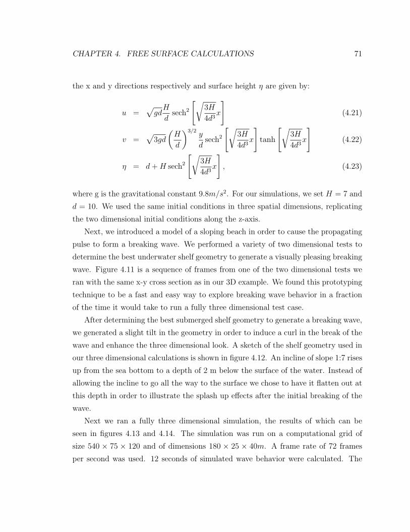
CHAPTER 4. FREE SURFACE CALCULATIONS 71
the x and y directions respectively and surface height η are given by:
u =√
gdH
dsech2
[√3H
4d3x
](4.21)
v =√
3gd
(H
d
)3/2y
dsech2
[√3H
4d3x
]tanh
[√3H
4d3x
](4.22)
η = d + H sech2
[√3H
4d3x
], (4.23)
where g is the gravitational constant 9.8m/s2. For our simulations, we set H = 7 and
d = 10. We used the same initial conditions in three spatial dimensions, replicating
the two dimensional initial conditions along the z-axis.
Next, we introduced a model of a sloping beach in order to cause the propagating
pulse to form a breaking wave. We performed a variety of two dimensional tests to
determine the best underwater shelf geometry to generate a visually pleasing breaking
wave. Figure 4.11 is a sequence of frames from one of the two dimensional tests we
ran with the same x-y cross section as in our 3D example. We found this prototyping
technique to be a fast and easy way to explore breaking wave behavior in a fraction
of the time it would take to run a fully three dimensional test case.
After determining the best submerged shelf geometry to generate a breaking wave,
we generated a slight tilt in the geometry in order to induce a curl in the break of the
wave and enhance the three dimensional look. A sketch of the shelf geometry used in
our three dimensional calculations is shown in figure 4.12. An incline of slope 1:7 rises
up from the sea bottom to a depth of 2 m below the surface of the water. Instead of
allowing the incline to go all the way to the surface we chose to have it flatten out at
this depth in order to illustrate the splash up effects after the initial breaking of the
wave.
Next we ran a fully three dimensional simulation, the results of which can be
seen in figures 4.13 and 4.14. The simulation was run on a computational grid of
size 540 × 75 × 120 and of dimensions 180 × 25 × 40m. A frame rate of 72 frames
per second was used. 12 seconds of simulated wave behavior were calculated. The

CHAPTER 4. FREE SURFACE CALCULATIONS 72
wave has the intended curling effect. The formation of a tube of air is clearly seen
after the wave splashes down, with the “air” particles maintaining the tube even after
the wave begins a secondary splash up. We observe some solely three dimensional
effects including the fingering of the breaking wave. The fine detail features seen
on the surface of the ocean surface, including the appearance of capillary waves and
foam were generated through the use of procedural displacement textures and matte
texture maps respectively. In order to simulate these details one would need to use
a finer computational grid along with a different velocity advection scheme than the
diffusive semi-Lagrangian method used here. However, for the purposes of computer
graphics we can use other methods besides physically-based animation techniques in
order to obtain plausible looking fine details to place on the wave. The goal of this
simulation was to show that the hard-to-animate bulk motion of the interface can be
obtained by using relatively simple algorithms from the computational fluid dynamics
community. The computational cost of this simulation was approximately 13 minutes
per frame.
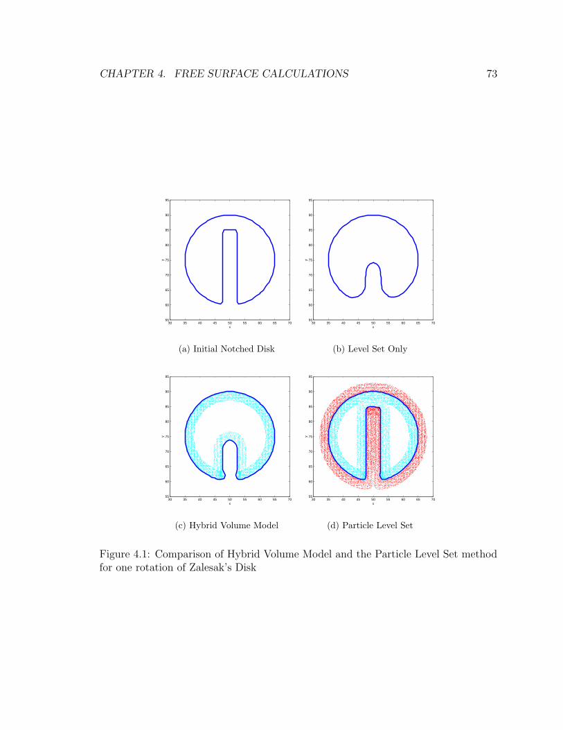
CHAPTER 4. FREE SURFACE CALCULATIONS 73
30 35 40 45 50 55 60 65 7055
60
65
70
75
80
85
90
95
x
y
(a) Initial Notched Disk
30 35 40 45 50 55 60 65 7055
60
65
70
75
80
85
90
95
x
y
(b) Level Set Only
30 35 40 45 50 55 60 65 7055
60
65
70
75
80
85
90
95
x
y
(c) Hybrid Volume Model
30 35 40 45 50 55 60 65 7055
60
65
70
75
80
85
90
95
x
y
(d) Particle Level Set
Figure 4.1: Comparison of Hybrid Volume Model and the Particle Level Set methodfor one rotation of Zalesak’s Disk
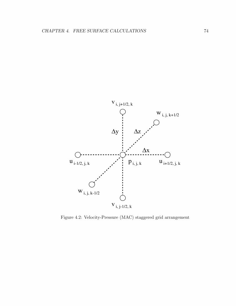
CHAPTER 4. FREE SURFACE CALCULATIONS 74
v i, j+1/2, k
u i-1/2, j, k u i+1/2, j, k
v i, j-1/2, k
w i, j, k+1/2
w i, j, k-1/2
p i, j, k
∆x
∆y ∆z
Figure 4.2: Velocity-Pressure (MAC) staggered grid arrangement
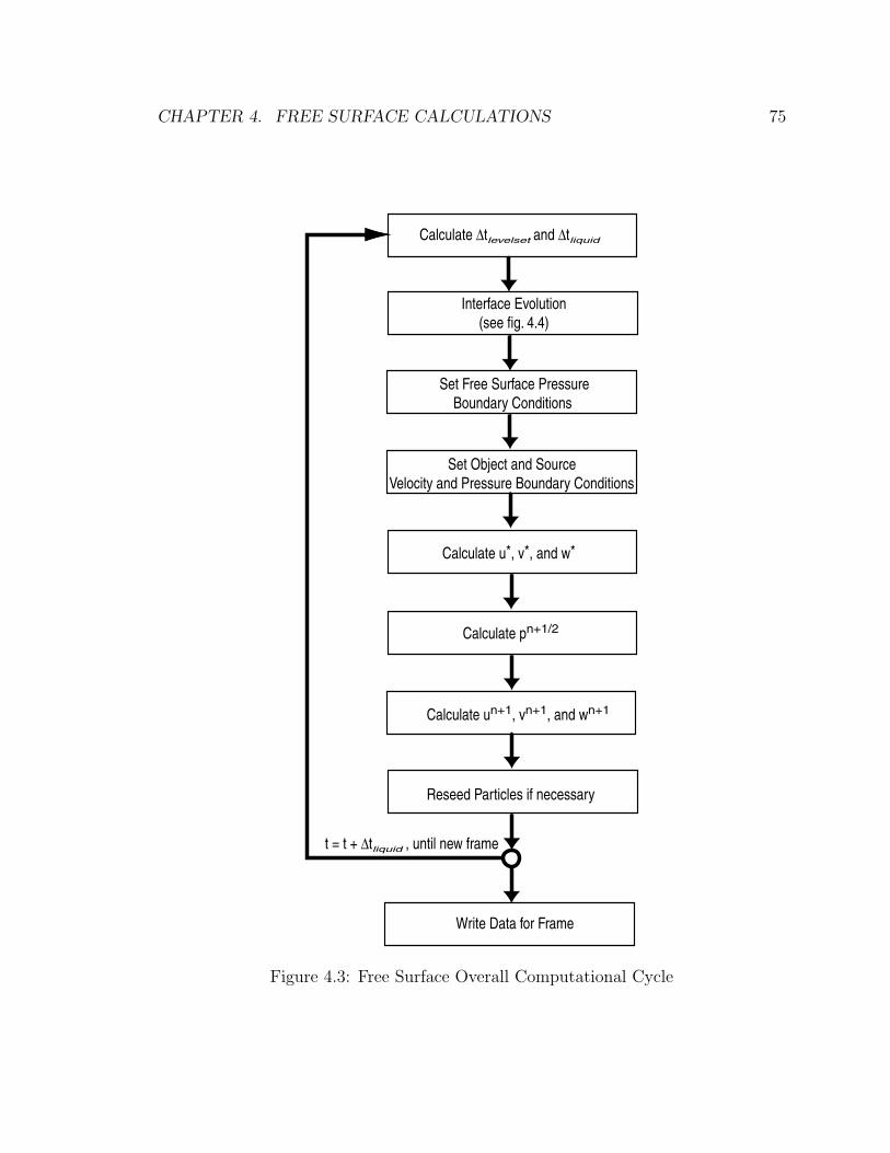
CHAPTER 4. FREE SURFACE CALCULATIONS 75
Calculate ∆tlevelset and ∆tliquid
Set Free Surface Pressure Boundary Conditions
Interface Evolution (see fig. 4.4)
Set Object and Source Velocity and Pressure Boundary Conditions
Calculate u*, v*, and w*
Calculate pn+1/2
Reseed Particles if necessary
Calculate un+1, vn+1, and wn+1
t = t + ∆tliquid , until new frame
Write Data for Frame
Figure 4.3: Free Surface Overall Computational Cycle
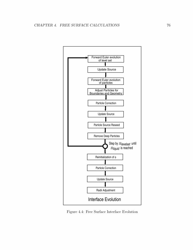
CHAPTER 4. FREE SURFACE CALCULATIONS 76
Forward Euler evolution of level set
Particle Correction
Update Source
Particle Source Reseed
Remove Deep Particles
Step by ∆tlevelset until ∆tliquid is reached
Interface Evolution
Update Source
Adjust Particles for Boundaries and Geometry
Forward Euler evolution of particles
Reinitialization of φ
Particle Correction
Radii Adjustment
Update Source
Figure 4.4: Free Surface Interface Evolution
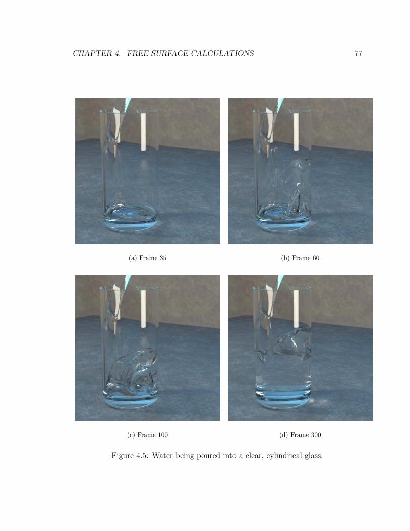
CHAPTER 4. FREE SURFACE CALCULATIONS 77
(a) Frame 35 (b) Frame 60
(c) Frame 100 (d) Frame 300
Figure 4.5: Water being poured into a clear, cylindrical glass.
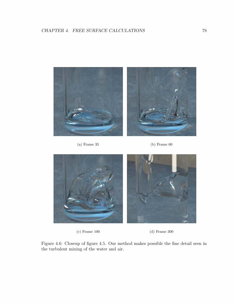
CHAPTER 4. FREE SURFACE CALCULATIONS 78
(a) Frame 35 (b) Frame 60
(c) Frame 100 (d) Frame 300
Figure 4.6: Closeup of figure 4.5. Our method makes possible the fine detail seen inthe turbulent mixing of the water and air.
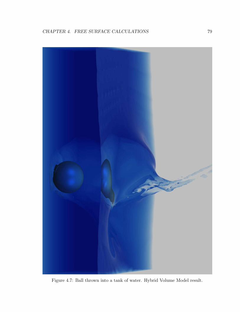
CHAPTER 4. FREE SURFACE CALCULATIONS 79
Figure 4.7: Ball thrown into a tank of water. Hybrid Volume Model result.
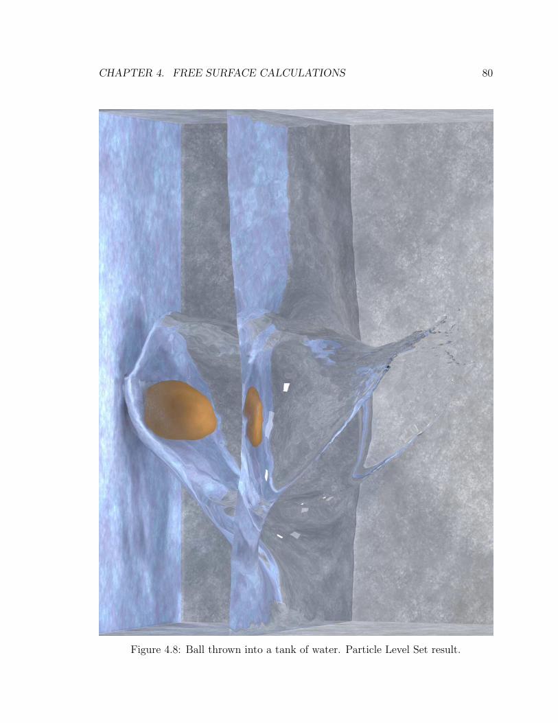
CHAPTER 4. FREE SURFACE CALCULATIONS 80
Figure 4.8: Ball thrown into a tank of water. Particle Level Set result.
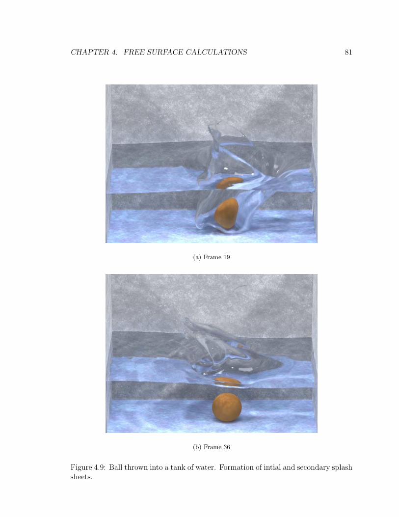
CHAPTER 4. FREE SURFACE CALCULATIONS 81
(a) Frame 19
(b) Frame 36
Figure 4.9: Ball thrown into a tank of water. Formation of intial and secondary splashsheets.
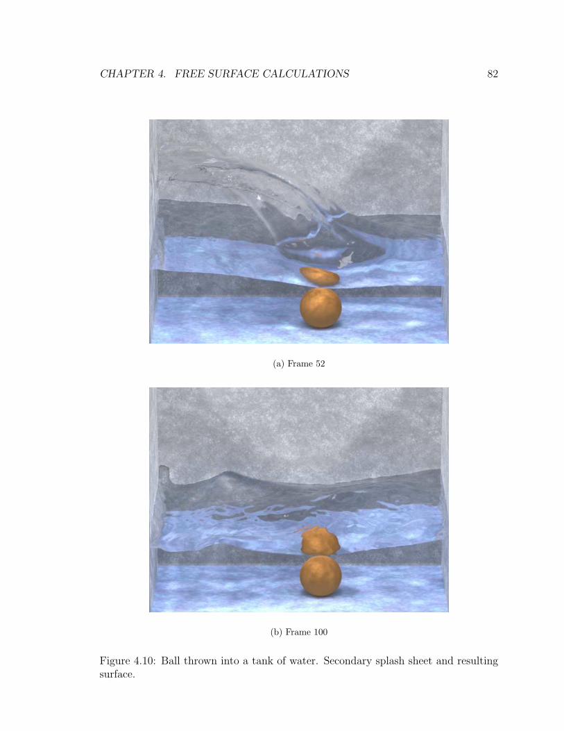
CHAPTER 4. FREE SURFACE CALCULATIONS 82
(a) Frame 52
(b) Frame 100
Figure 4.10: Ball thrown into a tank of water. Secondary splash sheet and resultingsurface.
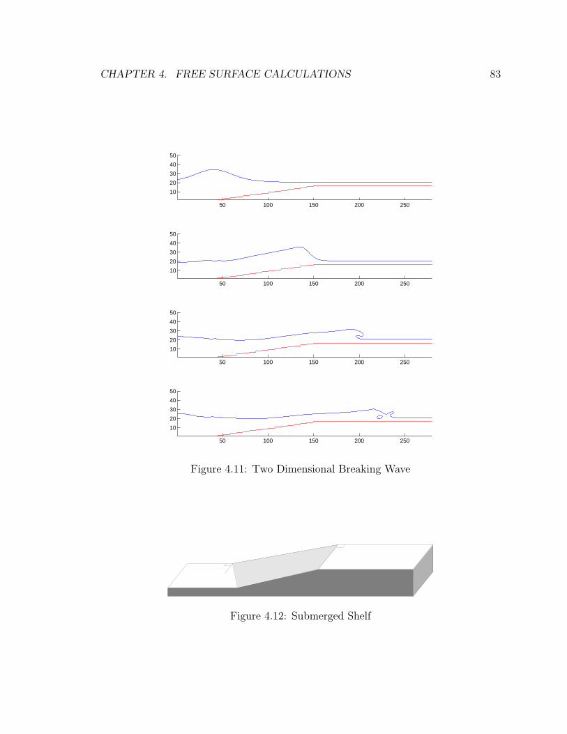
CHAPTER 4. FREE SURFACE CALCULATIONS 83
50 100 150 200 250
10
20
30
40
50
50 100 150 200 250
10
20
30
40
50
50 100 150 200 250
10
20
30
40
50
50 100 150 200 250
10
20
30
40
50
Figure 4.11: Two Dimensional Breaking Wave
Figure 4.12: Submerged Shelf
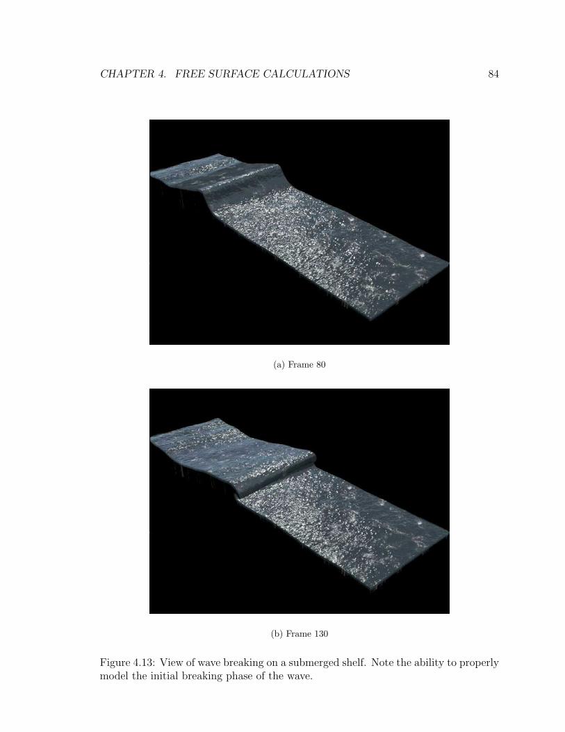
CHAPTER 4. FREE SURFACE CALCULATIONS 84
(a) Frame 80
(b) Frame 130
Figure 4.13: View of wave breaking on a submerged shelf. Note the ability to properlymodel the initial breaking phase of the wave.
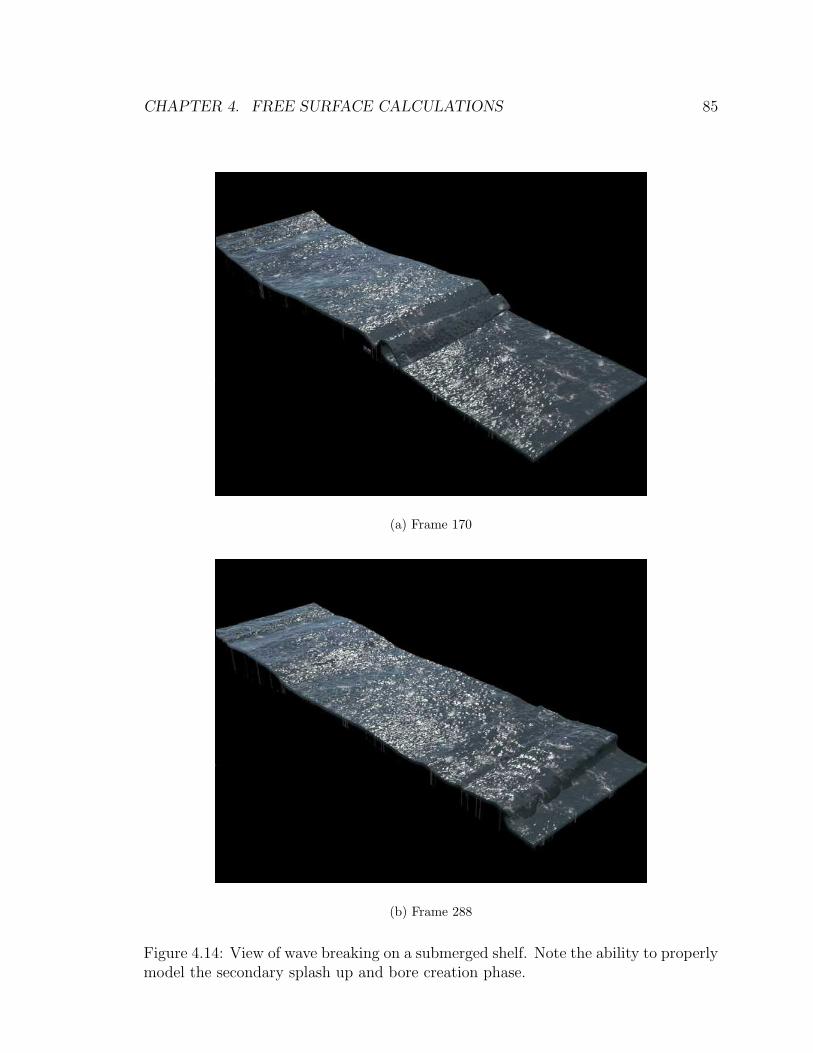
CHAPTER 4. FREE SURFACE CALCULATIONS 85
(a) Frame 170
(b) Frame 288
Figure 4.14: View of wave breaking on a submerged shelf. Note the ability to properlymodel the secondary splash up and bore creation phase.

Chapter 5
Conclusions and Future Directions
We have proposed a new numerical method which combines the best aspects of Eu-
lerian front capturing schemes and Lagrangian front tracking methods for improved
mass conservation. Level set methods are used to capture the smooth part of the
interface, but suffer an excessive amount of mass loss in under-resolved regions. This
prevents the resolution of thin filaments and regions of high curvature. To counter-
act this problem, characteristic information is provided by massless marker particles.
Escaped massless marker particles are used to correct the mass loss in the level set
function. The method otherwise maintains the desirable geometric properties of level
set methods along with the ease and simplicity of implementation. As seen in the
examples contained in chapter 3, the “particle level set method” compares favor-
ably with volume of fluid methods with regards to conservation of mass and purely
Lagrangian schemes for interface resolution.
While we add particles in a band near the interface, other strategies could be
adopted. For example, it is obvious that particles are only needed in regions of
high curvature and restricting particles to these regions would speed up the method
significantly. Concerning speed, it is interesting to compare this method to adaptive
meshing, for example as in [81]. A significant advantage of particle methods is that
they avoid the small time step restriction dictated by the small cells produced by
adaptive meshing. Also, the data structures are simpler than for cell based adaptive
meshing, and the particle method can be applied more locally than patch based
86
CHAPTER 5. CONCLUSIONS AND FUTURE DIRECTIONS 87
adaptive meshing.
We combined the “particle level set method” with a liquid free surface simulation
code in order to gauge the effectiveness of this method in maintaining a topologically
complex liquid interface in a computer animation environment. In order to use this
method, we took advantage of a well known tool in the level set community, velocity
extrapolation, in order to obtain a smooth, divergence free velocity field in the “air”
region near the interface. We performed three different animations, the pouring of
a glass of water, the splash formed due to the impact of a ball thrown into a tank
of water, and of a three dimensional, breaking surface wave. While breaking wave
calculations have been performed for some time in the computational fluid dynamics
community, see [48], this is the first time in an animation context that a breaking
wave calculation has been performed. The “particle level set method” combined with
velocity extrapolation near the interface appears to be a robust interface technique
in order to perform liquid animations on the coarse computational grids commonly
used in a production environment.
Future work includes using the “particle level set method” in order to calculate
enhanced resolution simulations of a variety of free surface flows including capillary jet
break up, the turbulent mixing resulting from plunging water waves, and the motion
of bubbles and drops. Extending the method to simulate the formation and evolution
of interfaces comprised of multiple immiscible fluids (such as those flows consisting of
air, oil, and water) [98, 99] would be challenging and of practical engineering interest.
An economically important application of the method would be the robust simulation
of the turbulent flow along the hull and behind the stern of a ship. There exists
complex physical processes including the breaking water waves, spray formation, and
free-surface turbulence. All of these phenomena contribute to the resistance that a
ship feels while moving through a body of water. Examples of ongoing work in this
area can be found in [22, 82]. By being able to experiment on a computer using
an accurate and robust Cartesian based method like the “particle level set method”,
different hull designs can be tested to see which produce the least drag.
While it has been demonstrated that the “particle level set method” is an effec-
tive method to track contact discontinuities, one of the applications which motivated
CHAPTER 5. CONCLUSIONS AND FUTURE DIRECTIONS 88
the creation of the method is the multidimensional aircraft collision avoidance cal-
culations performed by Mitchell and Tomlin [89, 54]. In this application where the
dimensionality of the PDE used is commonly higher than any flow calculation, a level
set method is used to determine the safe sets for aircraft control systems in order to
avoid collision. Due to the large number of degrees of freedom, the computational
grid used is fairly coarse and, as a result, controlling the amount of numerical diffu-
sion is of great concern. Particle methods have been used to sample a finite number
of states, which provides a very crude approximation of the overall safe set. Since the
governing equation for the evolution of the level set in this application is a discontinu-
ous Hamilton-Jacobi equation instead of an advection equation, this equation admits
not only contact discontinuities but also shocks and rarefactions. As illustrated in
chapter 1, particles are unable to capture the proper viscosity solution in the presence
of shocks in the flow field. One future goal is to modify the particle level set method
in order to make the error correction step a two-way process, in the case of a contact
discontinuity the particles propagate error information to the level set and vice versa
in the case of shocks.

Bibliography
[1] Adalsteinsson, D. and Sethian, J., A Fast Level Set Method for Propagating
Interfaces , J. Comp. Phys. 118, 269–277 (1995).
[2] Adalsteinsson, D. and Sethian, J., The Fast Construction of Extension Velocities
in Level Set Methods , J. Comp. Phys. 148, 2–22 (1999).
[3] Agresar, G., Linderman, J., Tryggvason, G. and Powell, K., An Adaptive, Carte-
sian, Front-Tracking Method for the Motion, Deformation and Adhesion of Cir-
culating Cells , J. Comp. Phys. 143, 346–380 (1998).
[4] Aleinov, I., Puckett, E. and Sussman, M., Formation of Droplets in Microscale
Jetting Devices , in Proceedings of the Third ASME/JSME Joint Fluids Engi-
neering Conference, FEDSM99-7106 , 1999.
[5] Amsden, A., Numerical Calculation of Surface Waves: A Modified ZUNI Code
with Surface Particles and Partial Cells , Technical Report LA-5146, Los Alamos
Scientific Laboratory (1973).
[6] Amsden, A. and Harlow, F., The SMAC Method: A Numerical Technique for
Calculating Incompressible Fluid Flows , Technical Report LA–4370, Los Alamos
Scientific Laboratory (1970).
[7] Baker, G. R., Meiron, D. I. and Orszag, S. A., Generalized vortex methods for
free-surface flow problems , J. Fluid Mech. 123, 477–501 (1982).
[8] Bell, J., Colella, P. and Glaz, H., A Second-Order Projection Method for the
Incompressible Navier-Stokes Equations , J. Comp. Phys. 85, 257–283 (1989).
89

BIBLIOGRAPHY 90
[9] Briggs, W. L., A Multigrid Tutorial , SIAM, Philadelphia, PA, 1987.
[10] Caiden, R., Fedkiw, R. and Anderson, C., A Numerical Method For Two-Phase
Flow Consisting of Separate Compressible and Incompressible Regions , J. Comp.
Phys. 166, 1–27 (2001).
[11] Cerne, G., Petelin, S. and Tiselj, I., Coupling of the Interface Tracking and
the Two-Fluid Models for the Simulation of Incompressible Two-Phase Flow , J.
Comp. Phys. 171, 776–804 (2001).
[12] Chan, R. K.-C. and Street, R. L., A Computer Study of Finite-Amplitude Water
Waves , J. Comp. Phys. 6, 68–94 (1970).
[13] Chang, Y., Hou, T., Merriman, B. and Osher, S., A Level Set Formulation of
Eulerian Inteface Capturing Methods for Incompressible Fluid Flows , J. Comp.
Phys. 124, 449–464 (1996).
[14] Chen, J. and Lobo, N., Toward Interactive-Rate Simulation of Fluids with Moving
Obstacles Using the Navier-Stokes Equations , Computer Graphics and Image
Processing 57, 107–116 (1994).
[15] Chen, S., Johnson, D. and Raad, P., Velocity Boundary Conditions for the Sim-
ulation of Free Surface Fluid Flow , J. Comp. Phys. 116, 262–276 (1995).
[16] Chen, S., Johnson, D., Raad, P. and Fadda, D., The Surface Marker and Micro
Cell Method , Int. J. for Num. Meth. in Fluids 25, 749–778 (1997).
[17] Chopp, D. L., Some Improvements of the Fast Marching Method , SIAM J. Sci.
Comput. 23, 230–244 (2002).
[18] Chorin, A. J., Numerical Solution of the Navier-Stokes Equations , Math. Comp.
22, 745–762 (1968).
[19] Cottet, G.-H. and Koumoutsakos, P. D., Vortex Methods , Cambridge Univ.
Press, Cambridge, UK, 2000.
BIBLIOGRAPHY 91
[20] Courant, R., Issacson, E. and Rees, M., On the Solution of Nonlinear Hyperbolic
Differential Equations by Finite Differences , Comm. Pure and Applied Math 5,
243–255 (1952).
[21] DeBar, R., A Method in Two-D Eulerian Hydrodynamics , Technical Report
UCID-19683, Lawrence Livermore National Laboratory (1974).
[22] Farmer, J., Martinelli, L. and Jameson, A., Fast Multigrid Method for Solving
Incompressible Hydrodynamic Problems with Free Surfaces , AIAA Jounral 32,
1175–1182 (1994).
[23] Fedkiw, R. P., Aslam, T., Merriman, B. and Osher, S., A Non-oscillatory Eule-
rian Approach to Interfaces in Multimaterial Flows (The Ghost Fluid Method),
J. Comp. Phys. 152, 457–492 (1999).
[24] Foster, N. and Fedkiw, R., Practical Animation of Liquids , in Fiume, E., ed.,
Proceedings of SIGGRAPH 2001 , Computer Graphics Proceedings, Annual Con-
ference Series, pp. 23–30, ACM, ACM Press / ACM SIGGRAPH, 2001.
[25] Foster, N. and Metaxas, D., Realistic Animation of Liquids , Graphical Models
and Image Processing 58, 471–483 (1996).
[26] Fournier, A. and Reeves, W. T., A Simple Model of Ocean Waves , in Computer
Graphics (Proceedings of SIGGRAPH 86), 20(4), pp. 75–84, ACM, 1986.
[27] Glassner, A., Principles of Digital Image Synthesis , Morgan Kaufmann Publish-
ers, Inc., San Francisco, CA, 1995.
[28] Golub, G. H. and Loan, C. F. V., Matrix Computations , Johns Hopkins Univer-
sity Press, Baltimore, MD, 1996, 3rd edition.
[29] Grilli, S. T., Guyenne, P. and Dias, F., A fully non-linear model for three-
dimensional overturning waves over an arbitrary bottom, Int. J. for Num. Meth.
in Fluids 35, 829–867 (2001).
BIBLIOGRAPHY 92
[30] Harlow, F., Shannon, J. and Welch, J., THE MAC METHOD: A Computing
Technique for Solving Viscous, Incompressible, Transient Fluid-Flow Problems
Involving Free Surfaces , Technical Report LA-3425, Los Alamos Scientific Lab-
oratory (1965).
[31] Harlow, F. and Welch, J., Numerical Calculation of Time-Dependent Viscous
Incompressible Flow of Fluid with Free Surface, Phys. Fluids 8, 2182–2189 (1965).
[32] Helmsen, J., A Comparison of Three-Dimensional Photolithography Development
Methods , Ph.D. thesis, U.C. Berkeley (1994).
[33] Hiltzik, M. A. and Pham, A., Synthetic Actors Guild , Los Angeles Times (2001),
may 8, 2001, natl. ed. : A1+.
[34] Hirt, C. and Nichols, B., Volume of Fluid (VOF) Method for the Dynamics of
Free Boundaries , J. Comp. Phys. 39, 201–225 (1981).
[35] Hirt, C. and Shannon, J., Free-Surface Stress Conditions for Incompressible-Flow
Calculations , J. Comp. Phys. 2, 403–411 (1968).
[36] Hou, T., Lowengrub, J. and Shelley, M., Boundary Integral Methods for Mul-
ticomponent Fluids and Multiphase Materials , J. Comp. Phys. 169, 302–362
(2001).
[37] Hou, T. Y., Numerical Solutions to Free Boundary Problems , Acta Numerica pp.
335–415 (1995).
[38] Jensen, H. W., Realistic Image Synthesis Using Photon Maps , A K Peters, 2001.
[39] Jiang, G.-S. and Peng, D., Weighted ENO Schemes for Hamilton-Jacobi Equa-
tions , SIAM J. Sci. Comput. 21, 2126–2143 (2000).
[40] Johnsgard, H., A Numerical Model for Run-Up of Breaking Waves , Int. J. for
Num. Meth. in Fluids 31, 1321–1331 (1999).
[41] Kang, M., Fedkiw, R. and Liu, X.-D., A Boundary Condition Capturing Method
for Multiphase Incompressible Flow , J. Sci. Comput. 15, 323–360 (2000).

BIBLIOGRAPHY 93
[42] Kass, M. and Miller, G., Rapid, Stable Fluid Dynamics for Computer Graphics ,
in Computer Graphics (Proceedings of SIGGRAPH 90), volume 24, pp. 49–57,
ACM, 1990.
[43] Kim, I. and Sirignano, W. A., Three-dimensional wave distortion and disintegra-
tion of thin planar liquid sheets , J. Fluid Mech. 410, 147–183 (2000).
[44] Kim, J. and Moin, P., Application of a fractional-step method to incompressible
Navier-Stokes equations , J. Comp. Phys. 59, 308–323 (1985).
[45] Lafaurie, B., Nardone, C., Scardovelli, R., Zaleski, S. and Zanetti, G., Modelling
Merging and Fragmentation in Multiphase Flows with SURFER, J. Comp. Phys.
113, 134–147 (1994).
[46] Lapenta, G. and Brackbill, J., Dynamic and Selective Control of the Number of
Particles in Kinetic Plama Simulations , J. Comp. Phys. 115, 213–227 (1994).
[47] Leveque, R., High-Resolution Conservative Algorithms For Advection In Incom-
pressible Flow , SIAM J. Numer. Anal. 33, 627–665 (1996).
[48] Longuet-Higgins, M. and Cokelet, E., The deformation of steep surface waves on
water. I. A numerical method of computation, Proc. R. Soc. London Ser. A 350,
1–26 (1976).
[49] Mansour, N. and Lundgren, T., Satellite formation in capillary jet breakup, Phys.
Fluids A 2, 1141–1144 (1990).
[50] Marschner, S. and Lobb, R., An Evaluation of Reconstruction Filters for Volume
Rendering , in Proceedings of Visualization 94 , pp. 100–107, IEEE Comput. Soc.
Press, 1994.
[51] Masten, G., Watterberg, P. and Mareda, I., Fourier Synthesis of Ocean Scenes ,
IEEE Computer Graphics and Application 7, 16–23 (1987).
[52] McDonald, A., Accuracy of Multiply-Upstream, Semi-Lagrangian Advective
Schemes , Monthly Weather Review 112, 1267–1275 (1982).

BIBLIOGRAPHY 94
[53] Miller, G. and Pearce, A., Globular Dynamics: A Connected Particle System for
Animating Viscous Fluids , Computers and Graphics 13(3), 305–309 (1989).
[54] Mitchell, I. and Tomlin, C., Level Set Methods for Computation in Hybrid Sys-
tems , in Krogh, B. and Lynch, N., eds., Hybrid Systems: Computation and
Control , pp. 310–323, Springer Verlag, 2000.
[55] Nguyen, D. Q., Fedkiw, R. P. and Kang, M., A Boundary Condition Capturing
Method for Incompressible Flame Discontinuities , J. Comp. Phys. 172, 71–98
(2001).
[56] Nichols, B. and Hirt, C., Improved Free Surface Boundary Conditions for Nu-
merical Incompressible-flow Calculations , J. Comp. Phys. 8, 434–448 (1971).
[57] O’Brien, J. and Hodgins, J., Dynamic Simulation of Splashing Fluids , in Pro-
ceedings of Computer Animation 95 , pp. 198–205, 1995.
[58] Osher, S. and Fedkiw, R., Level Set Methods: An Overview and Some Recent
Results , J. Comp. Phys. 169, 463–502 (2001).
[59] Osher, S. and Fedkiw, R., The Level Set Method and Dynamic Implicit Surfaces ,
Springer-Verlag, New York, 2002.
[60] Osher, S. and Sethian, J., Fronts Propagating with Curvature Dependent Speed:
Algorithms Based On Hamiliton-Jacobi Formulations , J. Comp. Phys. 79, 12–49
(1988).
[61] Peachey, D. R., Modeling Waves and Surf , in Computer Graphics (Proceedings
of SIGGRAPH 86), 20(4), pp. 65–74, ACM, 1986.
[62] Peng, D., Merriman, B., Osher, S., Zhao, H.-K. and Kang, M., A PDE-Based
Fast Local Level Set Method , J. Comp. Phys. 155, 410–438 (1999).
[63] Puckett, E., Almgren, A., Bell, J., Marcus, D. and Rider, W., A High-Order Pro-
jection Method for Tracking Fluid Interfaces in Variable Density Incompressible
Flows , J. Comp. Phys. 130, 269–282 (1997).
BIBLIOGRAPHY 95
[64] Raad, P., Chen, S. and Johnson, D., The Introduction of Micro Cells to Treat
Pressure in Free Surface Fluid Flow Problems , J. Fluids Eng. 117, 683–690
(1995).
[65] Radovitzky, R. and Ortiz, M., Lagrangian Finite Element Analysis of Newtonian
Fluid Flows , Int. J. Numer. Meth. Engng. 43, 607–619 (1998).
[66] Rider, W. and Kothe, D., A Marker Particle Method for Interface Tracking , in
Dwyer, H., ed., Proceedings of the Sixth International Symposium on Computa-
tional Fluid Dynamics , pp. 976–981, 1995.
[67] Rider, W. and Kothe, D., Stretching and Tearing Interface Tracking Methods , in
12th AIAA CFD Conference, 95–1717, AIAA, 1995.
[68] Rider, W. and Kothe, D., Reconstructing Volume Tracking , J. Comp. Phys. 141,
112–152 (1998).
[69] Schachter, B., Long Crested Wave Models , Computer Graphics and Image Pro-
cessing 12, 187–201 (1980).
[70] Sethian, J., Curvature and the Evolution of Fronts , Comm. Math. Phys. 101,
487–499 (1985).
[71] Sethian, J., Numerical Methods for Propagating Fronts , in Concus, P. and Finn,
R., eds., Variational Methods for Free Surface Interfaces , Springer-Verlag, 1987.
[72] Sethian, J., A Fast Marching Level Set Method for Monotonically Advancing
Fronts , Proc. Natl. Acad. Sci. 93, 1591–1595 (1996).
[73] Sethian, J., Fast Marching Methods , SIAM Rev. 41, 199–235 (1999).
[74] Sethian, J., Level Set Methods and Fast Marching Methods , Cambridge Univer-
sity Press, 1999.
[75] Sethian, J., Evolution, Implementation, and Application of Level Set and Fast
Marching Methods for Advancing Fronts , J. Comp. Phys. 169, 503–555 (2001).

BIBLIOGRAPHY 96
[76] Shu, C. and Osher, S., Efficient Implementation of Essentially Non-Oscillatory
Shock Capturing Schemes , J. Comp. Phys. 77, 439–471 (1988).
[77] Smolarkiewicz, P., The Multi-Dimensional Crowley Advection Scheme, Monthly
Weather Review 110, 1968–1983 (1982).
[78] Stam, J., Stable Fluids , in Proceedings of SIGGRAPH 99 , Computer Graphics
Proceedings, Annual Conference Series, pp. 121–128, ACM, ACM SIGGRAPH
/ Addison Wesley Longman, 1999.
[79] Staniforth, A. and Cote, J., Semi-Lagrangian Integration Schemes for Atmo-
spheric Models - A Review , Montly Weather Review 119, 2206–2223 (1991).
[80] Sussmam, M. and Puckett, E., A Coupled Level Set and Volume-of-Fluid Method
for Computing 3D and Axisymmetric Incompressible Two-Phase Flows , J. Comp.
Phys. 162, 301–337 (2000).
[81] Sussman, M., Almgren, A., Bell, J., Colella, P., Howell, L. and Welcome, M.,
An Adaptive Level Set Approach for Incompressible Two-Phase Flows , J. Comp.
Phys. 148, 81–124 (1999).
[82] Sussman, M. and Dommermuth, D., The Numerical Simulation of Ship Waves
Using Cartesian Grid Methods , in Twenty-Third Symposium on Naval Hydrody-
namics , pp. 762–779, 2001.
[83] Sussman, M. and Fatemi, E., An Efficient, Interface-Preserving Level Set Redis-
tancing Algorithm and Its Application to Interfacial Incompressible Fluid Flow ,
SIAM J. Sci. Comput. 20, 1165–1191 (1999).
[84] Sussman, M., Fatemi, E., Smereka, P. and Osher, S., An Improved Level Set
Method for Incompressible Two-Phase Flows , Comput. and Fluids 27, 663–680
(1998).
[85] Sussman, M., Smereka, P. and Osher, S., A Level Set Approach for Comput-
ing Solutions to Incompressible Two-Phase Flow , J. Comp. Phys. 114, 146–159
(1994).
BIBLIOGRAPHY 97
[86] Terzopoulos, D., Platt, J. and Fleischer, K., Heating and melting deformable
models (From goop to glop), in Graphics Interface ’89 , pp. 219–226, 1989.
[87] Tome, M., Filho, A., Cuminato, J., Mangiavacchi, N. and McKee, S., GENS-
MAC3D: a numerical method for solving unsteady three-dimensional free surface
flows , Int. J. for Num. Meth. in Fluids 37, 747–796 (2001).
[88] Tome, M., McKee, S., Barratt, L., Jarvis, D. and Patrick, A., An Experimental
and Numerical Investigation of Container Filling With Viscous Liquids , Int. J.
for Num. Meth. in Fluids 31, 1333–1353 (1999).
[89] Tomlin, C., Mitchell, I. and Ghosh, R., Safety Verification of Conflict Resolution
Manoeuvres , IEEE Trans. Intell. Transp. Syst. 2, 110–120 (2001).
[90] Torres, D. and Brackbill, J., The Point-Set Method: Front Tracking without
Connectivity , J. Comp. Phys. 165, 620–644 (2000).
[91] Tryggvason, G., Bunner, B., Esmaeeli, A., Juric, D., Al-Rawahi, N., Tauber, W.,
Han, J., Nas, S. and Jan, Y.-J., A Front-Tracking Method for the Computations
of Multiphase Flow , J. Comp. Phys. 169, 708–759 (2001).
[92] Unverdi, S.-O. and Tryggvason, G., A Front-Tracking Method for Viscous, In-
compressible, Multi-fluid Flows , J. Comp. Phys. 100, 25–37 (1992).
[93] Williams, M., Kothe, D. and Puckett, E., Approximating Interfacial Topologies
with Applications for Interface Tracking Algorithms , in 37th AIAA Aerospace
Sciences Meeting , AIAA 99–1076, 1999.
[94] Williams, M., Kothe, D. and Puckett, E., Convergence and Accuracy of Kernal-
Based Continuum Surface Tension Models , in Shyy, W., ed., Fluid Dynamics at
Interfaces , pp. 347–356, Cambridge University Press, 1999.
[95] Witting, P., Computational Fluid Dynamics in a Traditional Animation Envi-
ronment , in Proceedings of SIGGRAPH 99 , Computer Graphics Proceedings,
Annual Conference Series, pp. 129–136, ACM, ACM SIGGRAPH / Addison
Wesley Longman, 1999.

BIBLIOGRAPHY 98
[96] Zalesak, S., Fully Multidimensional Flux-Corrected Transport Algorithms for Flu-
ids , J. Comp. Phys. 31, 335–362 (1979).
[97] Zhang, Y., Yeo, K., Khoo, B. and Wang, C., 3D Jet Impact and Toroidal Bubbles ,
J. Comp. Phys. 166, 336–360 (2001).
[98] Zhao, H.-K., Chan, T., Merriman, B. and Osher, S., A Variational Level Set
Approach to Multiphase Motion, J. Comp. Phys. 127, 179–195 (1996).
[99] Zhao, H.-K., Merriman, B., Osher, S. and Wang, L., Capturing the Behavior of
Bubbles and Drops Using the Variational Level Set Approach, J. Comp. Phys.
143, 495–518 (1998).