Using Calibration Weighting to Adjust

for Nonresponse Under a Plausible

Model (with full appendices)

Ted Chang

Department of Statistics, University of Virginia,

Charlottesville VA 22904-4135 USA

tcc8v@virginia.edu

Phillip S Kott

National Agricultural Statistical Service,

Fairfax VA 22030-1504 USA

Phil Kott@nass.usda.gov

Summary

Calibration forces the weighted estimates of certain variables to match known

or alternatively estimated population totals called benchmarks. It can be used to

correct for sample-survey nonresponse or for coverage error resulting from frame

undercoverage or unit duplication. The quasi-randomization theory supporting its

use in nonresponse adjustment treats response as an additional phase of random

sampling. The functional form of a quasi-random response model is assumed to be

known, its parameter values estimated implicitly through the creation of calibra-

tion weights. Unfortunately, calibration depends upon known benchmark totals

1

while the variables in a plausible model for survey response are not necessarily

the same as the benchmark variables. Moreover, it may be prudent to keep the

number of explanatory variables in a response model small. We will address using

calibration to adjust for nonresponse when the explanatory model variables and

benchmark variables are allowed to differ as long as the number of benchmark

variables is at least as great as the number of model variables. Data from National

Agricultural Statistical Service’s 2002 Census of Agriculture and simulations based

upon that data will be used to illustrate alternative adjustments for nonresponse.

The paper concludes with some remarks about extension of the methodology to

adjustment for coverage error.

Some key words: Benchmark; Consistency; Coverage model; Back-link function; Quasi-

randomization; Response model.

1. Introduction

Calibration weighting ensures that sample-estimated totals of certain calibra-

tion or benchmark variables match previously determined population totals. Two

related special cases of calibration, poststratification and weighting-class adjust-

ment (see Lohr 1999, pp. 266-267) are used extensively to adjust for survey non-

response, a subject of growing interest as the response rates in both government

and private surveys decline.

Oh and Scheuren (1983) provide a theoretical justification for weighting-class

adjustment by treating response as a second phase of sample selection. In this

quasi-randomization (or quasi-design-based) framework, each sampled unit within

the same weighting class has an equal and independent probability of selection

into the respondent subsample. That probability is estimated implicitly in the

weighting process. The prefix “quasi” is added to “randomization” to emphasize

that inference is not model free, but depends on an assumed response model. Like

all models, the response model can fail. Unfortunately, any method for handling

2

nonresponse requires some form of modelling, at least implicitly.

More complex nonresponse adjusting calibration schemes are proposed in Fol-

som (1991), Fuller, Louglin, and Baker (1994), and Kott (2006). In each the

probability of response is assumed to be a known “back-link” function p(xTi β∗)

of an unknown (but estimatable) linear combination of explanatory model vari-

ables xi. The back-link function is the back transformation of the link function

in a generalized linear model. See, for example, McCullagh and Nelder (1989).

What we have called the “back-link” is sometimes called the “inverse link” in the

generalized-linear-model literature.

In Fuller et al., the back-link function has the form p(η) = 1/(1 + η). This

allows calibration to have its conventional linear form. Lundstrom and Sarndal

(1999) also proposes using calibration in conventional linear form to adjust for

nonresponse but without specifying a back-link function.

Folsom proposes more plausible functions for the modeling of response than

p(η) = 1/(1 + η). One such is the logistic: p(η) = [1 + exp(−η)]−1. In addition,

raking is shown to be a form of calibration weighting with a back-link function of

the form p(η) = exp(η). A follow-up, Folsom and Singh (2000), proposes a class

of reasonable back-link functions.

In both Fuller et al. and Folsom the explanatory model variables used to esti-

mate implicitly the probabilities of response are the same as the calibration vari-

ables for which one has benchmark totals. In Kott that is no longer the case. This

extension does not require that model-variable totals be known. For example, one

can separate respondents into response groups in an analogue to poststratification

based on their survey responses. Still, Kott assumes the number of explanatory

model and benchmark variables are equal. Moreover, that paper does not demon-

strate the practicality of its approach with data.

Sarndal and Lundstrom (2005) also treats the case where the explanatory model

and benchmark variables can differ in definition but not in number. In addition,

it allows some of the benchmark totals to be calculable from the sample before

3

nonresponse. The back-link function is not specified. Moreover, the authors do

not appear to notice that calibration is possible when model-variable values are

known only for the respondents.

We will show how to use calibration to adjust for nonresponse when the number

of benchmark variables is at least as great as the number of explanatory model

variables. As in Kott, the values for the explanatory variables need only be known

for respondents. In Section 2 we will introduce our notation and motivate our

approach to calibration, which is discussed in more detail in Sections 3 and 4.

In section 5 we turn to the estimation of a total for a vector of variables of

interest that typically do not include the benchmark variables (since they are

either already known or previously estimated) but may include some of the model

variables. We show how to measure both the additional asymptotic variance due

to the nonresponse in a calibration-weighted estimator and the full asymptotic

variance of the estimator itself. All variances in the text are determined either with

respect to the randomization mechanism used to select the sample, the response

model generating the subset of sample respondents, or both.

Section 6 contains applications of our methodology to nonresponse adjustment

for the 2002 Census of Agriculture. We show here how the probability of a farm’s

responding to the census can be assumed to be a function of its survey-reported

sales rather than its expected sales before enumeration, as is currently assumed

in practice. In section 7 we report on simulations from an artificial population

constructed from the respondents of the Census of Agriculture. These sections

also discuss the implications of a misspecified model.

Section 8 provides some concluding remarks. Among them is a brief discussion

about extending the findings of the preceding sections to adjusting for coverage

errors, a topic of increasing interest for surveys based on incomplete frames such

as telephone and internet surveys.

2. Notation and motivation

4

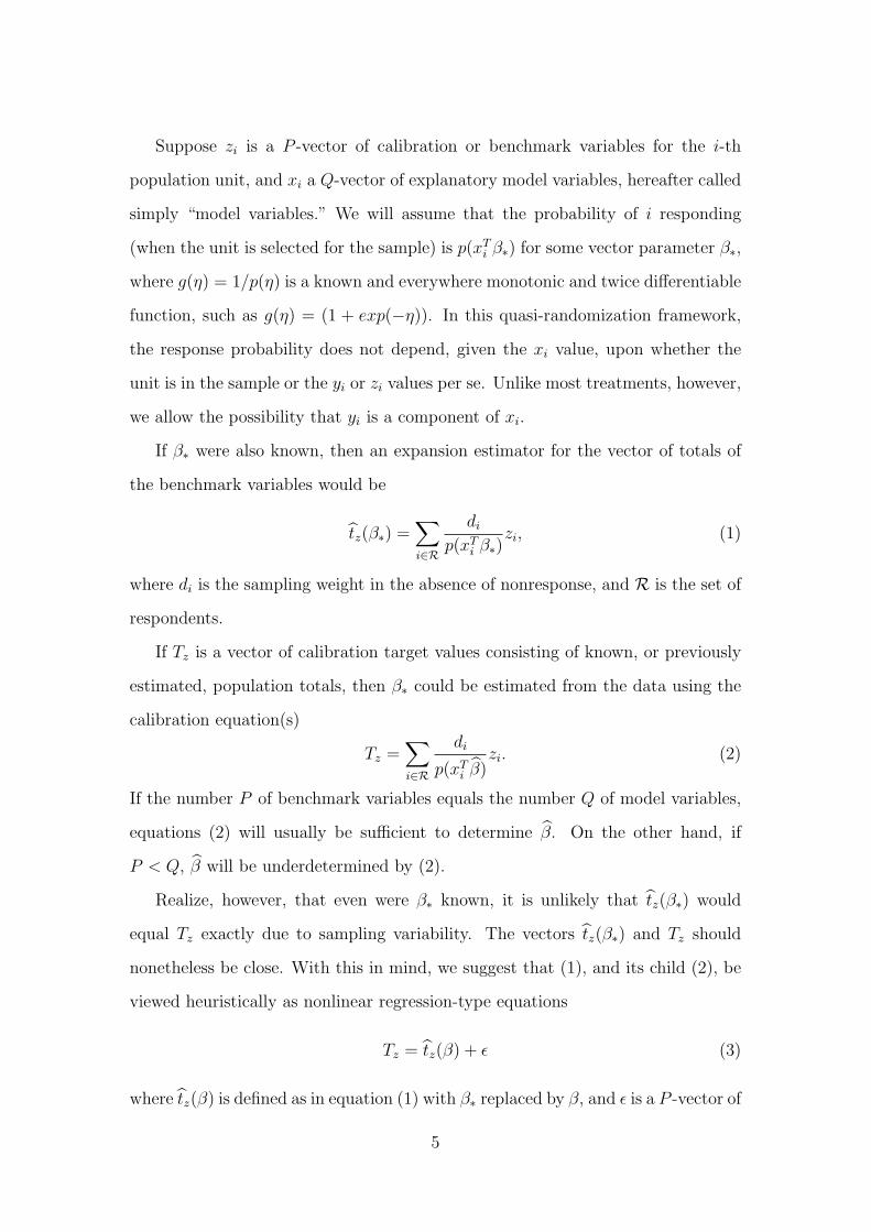
Suppose zi is a P -vector of calibration or benchmark variables for the i-th

population unit, and xi a Q-vector of explanatory model variables, hereafter called

simply “model variables.” We will assume that the probability of i responding

(when the unit is selected for the sample) is p(xTi β∗) for some vector parameter β∗,

where g(η) = 1/p(η) is a known and everywhere monotonic and twice differentiable

function, such as g(η) = (1 + exp(−η)). In this quasi-randomization framework,

the response probability does not depend, given the xi value, upon whether the

unit is in the sample or the yi or zi values per se. Unlike most treatments, however,

we allow the possibility that yi is a component of xi.

If β∗ were also known, then an expansion estimator for the vector of totals of

the benchmark variables would be

tz(β∗) =∑i∈R

di

p(xTi β∗)

zi, (1)

where di is the sampling weight in the absence of nonresponse, and R is the set of

respondents.

If Tz is a vector of calibration target values consisting of known, or previously

estimated, population totals, then β∗ could be estimated from the data using the

calibration equation(s)

Tz =∑i∈R

di

p(xTi β)

zi. (2)

If the number P of benchmark variables equals the number Q of model variables,

equations (2) will usually be sufficient to determine β. On the other hand, if

P < Q, β will be underdetermined by (2).

Realize, however, that even were β∗ known, it is unlikely that tz(β∗) would

equal Tz exactly due to sampling variability. The vectors tz(β∗) and Tz should

nonetheless be close. With this in mind, we suggest that (1), and its child (2), be

viewed heuristically as nonlinear regression-type equations

Tz = tz(β) + ε (3)

where tz(β) is defined as in equation (1) with β∗ replaced by β, and ε is a P -vector of

5

“errors”. In the nonlinear regression paradigm, it is desirable that P > Q. Indeed,

since each target provides an additional “equation” in (3), one would suspect that

addition of targets will improve the calibration as long as the additional targets

do not introduce correlation problems in the tz(β∗). More precise results in this

direction are a topic for future research.

The parameter β can be estimated by minimizing an objective function of the

form

ρ(β) = −logdet(W ) + (Tz − tz(β))T W (Tz − tz(β)) (4)

for some appropriately chosen P×P positive definite matrix W (which may depend

upon β), where logdet(W ) denotes the log of the determinant of W . Note that

(4) is the log likelihood of tz(β) under an asymptotic normal distribution with

covariance matrix W−1. In maximum likelihood estimation, where W is estimated

from the sample, the −logdet(W ) term prevents the minimization from attempting

to send W → 0. It is important to realize that when P > Q, no choice of β forces

tz(β) to equal Tz as in conventional P = Q calibration.

The nonlinear regression formulation of (3) suggests setting W = V −1 for some

suitably defined variance matrix V of ε. When this choice of W depends on β, we

propose an iterative procedure analogous to what would be used with a fixed W .

Given a guess β0 of β∗, we can linearize the regression (3) at β0. The solution to

the linearized regression is the next guess β1. This procedure is described more

thoroughly in Section 3.

An obvious candidate for V is varqr(tz(β)|β = β∗), an estimator for the quasi-

randomization variance of tz(β) assuming β = β∗. If the sampling scheme is

without replacement so that tz(β) of (3) is the Horvitz Thompson estimator, then

one such quasi-randomization variance estimator is

varqr(tz(β)|β = β∗) =∑i,j∈R

πij − πiπj

πijπiπjpipj

zizTj +

∑i∈R

1− pi

p2i πi

zizTi , (5)

where pi = p(xTi β). Equation (5) is derived in Appendix 1.

6

In the quasi-randomization framework supporting (5) one assumes the set R

of respondents results from a two-phase sample of the target population U . In the

first phase, the sample S is drawn without replacement from the population with

inclusion probabilities πi = Pr[ i ∈ S] and πij = Pr[ i, j ∈ S]. Note that πii = πi.

In this case, di = π−1i . In the second phase, R is a Poisson subsample of S with

unit selection probabilities of the form pi = p(xTi β).

If the targets Tz are themselves previously estimated population totals, then it

is reasonable to let

V = varqr(tz(β)|β = β∗) + var(Tz)

where var(Tz) is a good externally determined estimate of the variance of Tz. In

some applications var(Tz) may be much greater than varqr(tz(β)|β = β∗), in the

sense that the eigenvalues of var(Tz)− varqr(tz(β)|β = β∗) are large. In this case,

it would be reasonable to set W to (var(Tz))−1, which is not a function of β at all.

3. Partial minimization

Given a guess β0 of β and matrix W (β0) we linearize (3) at β0 and obtain

Tz − tz(β0) = tz(β)− tz(β0) + ε ≈ H(β0)(β − β0) + ε, (6)

where H(β0) is the Q× P matrix

H(β0) =∂tz(β)

∂β

∣∣∣β=β0

=∑i∈R

dig1(xTi β0)zix

Ti , (7)

and g1(xTi β0) is the first derivative of g(η) = 1/p(η) evaluated at xT

i β0.

The (weighted) linear regression estimate β1 corresponding to (6) minimizes

the objective function UT W (β0)U where U = Tz − tz(β0) − H(β0)(β − β0). It is

given by the “update equation”:

β1 = β0 +{

H(β0)T W (β0)H(β0)

}−1

H(β0)T W (β0)(Tz − tz(β0)) (8)

7

For simplicity, we assume H(β) and W (β) are of full rank everywhere. This will

allow us to always be able to invert matrices when the need arises.

Iteration continues with β1 serving the role of β0, and H and W updated to

β1, in (8), and so on until we reach a step K, if such a step can be reached, where

(at least to some small pre-specified tolerance)

HT W (Tz − tz(β)) = 0 (9)

with the matrices H and W evaluated at β = βK . As the iteration starting with

(8) is a Newton-Raphson type method, it is sometimes helpful to limit the size

of the step from, say, βk−1 to βk for some k = 1, ..., K. What this means is

that when{

H(βk−1)T W (βk−1)H(βk−1)

}−1 {H(βk−1)

T W (βk−1)(Tz − tz(βk−1))}

is

deemed too large, it can be replaced with some fraction of itself in the update

equation.

If W is the inverse of an estimate for the variance matrix of tz(β), an alternative

derivation and justification of the update equation (8) follows from Thompson

(1997), section 6.3. Consider the equations tz(β)−Tz = 0 as P estimating equations

for the Q coefficients β. If A is a Q × P matrix of constants, let βA denote the

solution to the estimating equations

Atz(β) = ATz. (10)

A choice for A such that βA has a minimum asymptotic variance is

A∗ = H(βA∗)Tvar(tz(βA∗))−1,

where βA∗ results from the convergence of update equation (8).

Observe that when W = W (β) depends upon β, our suggested procedure for

estimating β∗ does not minimize the objective function (4). This is because if (4)

were differentiated with respect to β, then there would be a term for the derivative

of W which is not accounted for in the linearization (6). In other words, letting

ρ(β, γ) = −logdet(W (γ)) + (Tz − tz(β))T W (γ)(Tz − tz(β)),

8

full minimization would solve the equation

0 =∂ρ

∂β(β, β) +

∂ρ

∂γ(β, β) (11)

whereas the partial minimization, obtained through iterated use of (8), sets only

the first term of the right hand side of (11) to zero. In what follows we will

distinguish partial minima from full minima by using the notation β for the former

and β for the latter.

In the appendices we first discuss an example of conditions sufficient to establish

the consistency of β under full minimization and then the asymptotic equivalence

of the partial minimum β. Full and partial minimization usually yielded very

similar results in our own empirical investigations, with the former taking longer

to compute. In fact, finding a full minimum was extremely difficult when there

was no partial-minimum solution to use as an initial guess in the iterative process

to full minimization. Given that, the asymptotic equality of the two minima, and

the reliance on an asymptotic framework in our analysis, most of the remainder of

text concerns partial-minimization results.

4. Some choices for W

When P = Q, equation (8) reduces to

β1 = β0 + H−1(Tz − tz(β0)). (12)

Thus, in this case, the form of W is irrelevant for the update equation. Indeed

(12) is the Newton-Raphson update equation for solving the equation Tz = tz(β),

and the solution, if it exists, will also minimize (4), at least for any W which does

not depend upon β.

When P > Q, we propose setting W (β) to the inverse of V = varqr(tz(β)|β =

β∗) + var(Tz), where the latter term is provided to us from external sources (and

may be 0). If the sample S is selected without replacement, then (5) is an unbiased

estimate of varqr(tz(β)|β = β∗).

9

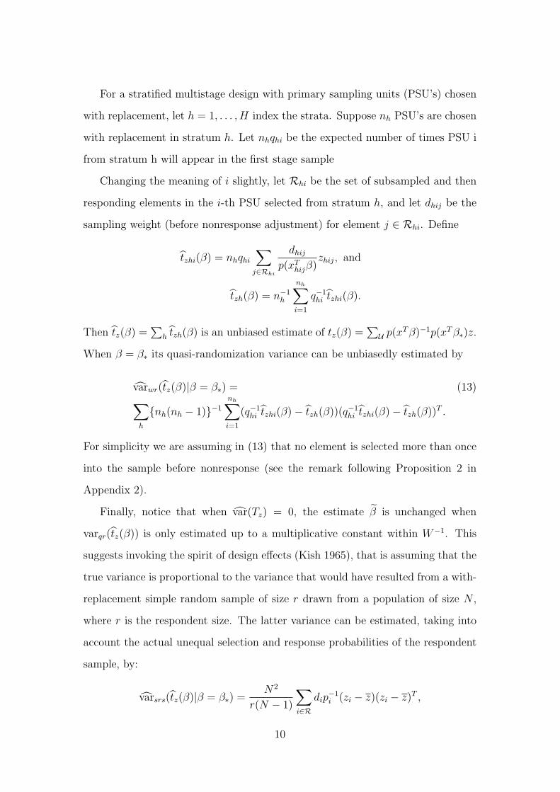
For a stratified multistage design with primary sampling units (PSU’s) chosen

with replacement, let h = 1, . . . , H index the strata. Suppose nh PSU’s are chosen

with replacement in stratum h. Let nhqhi be the expected number of times PSU i

from stratum h will appear in the first stage sample

Changing the meaning of i slightly, let Rhi be the set of subsampled and then

responding elements in the i-th PSU selected from stratum h, and let dhij be the

sampling weight (before nonresponse adjustment) for element j ∈ Rhi. Define

tzhi(β) = nhqhi

∑j∈Rhi

dhij

p(xThijβ)

zhij, and

tzh(β) = n−1h

nh∑i=1

q−1hi tzhi(β).

Then tz(β) =∑

h tzh(β) is an unbiased estimate of tz(β) =∑

U p(xT β)−1p(xT β∗)z.

When β = β∗ its quasi-randomization variance can be unbiasedly estimated by

varwr(tz(β)|β = β∗) = (13)∑h

{nh(nh − 1)}−1

nh∑i=1

(q−1hi tzhi(β)− tzh(β))(q−1

hi tzhi(β)− tzh(β))T .

For simplicity we are assuming in (13) that no element is selected more than once

into the sample before nonresponse (see the remark following Proposition 2 in

Appendix 2).

Finally, notice that when var(Tz) = 0, the estimate β is unchanged when

varqr(tz(β)) is only estimated up to a multiplicative constant within W−1. This

suggests invoking the spirit of design effects (Kish 1965), that is assuming that the

true variance is proportional to the variance that would have resulted from a with-

replacement simple random sample of size r drawn from a population of size N ,

where r is the respondent size. The latter variance can be estimated, taking into

account the actual unequal selection and response probabilities of the respondent

sample, by:

varsrs(tz(β)|β = β∗) =N2

r(N − 1)

∑i∈R

dip−1i (zi − z)(zi − z)T ,

10

where

z = (∑i∈R

dip−1i )−1

∑i∈R

dip−1i zi,

and, as before, pi = p(xTi β). In practice, the scalar multiple N2r−1(N − 1)−1 can

be dropped from V within W = V −1.

5. The calibration-weighted estimator for a population total and

its quasi-randomization variance

Let yi be a vector of variables of interest. The purpose of calibration weighting

is to estimate population totals for the components of yi or functions of those

totals, like population ratios. Typically, the components of yi will not include the

benchmark variables in zi as the latter’s totals are already known or have been

alternatively estimated. They may include model variables in xi. In principle,

however, they could include both types of variables.

Our calibration-weighted estimator for the total ty is

ty(β) =∑i∈R

di

p(xTi β)

yi =∑i∈R

dig(xTi β)yi =

∑i∈R

ciyi, (14)

where ci = dig(xTi β) is the calibration weight for unit i. Define

Hy =∂ty∂β

(β) =∑i∈R

dig1(xTi β)yix

Ti , and

B = Hy(HT WH)−1HT W,

where H = Hz is the matrix of partial derivatives (7) which, like W , is evaluated

at β. Note that the components of Hy/N are OP (1).

Writing yi as Bzi + (yi −Bzi), we have

ty(β) = Btz(β) +∑i∈R

di

p(xTi β)

(yi −Bzi)

= BTz +∑i∈R

dig(xTi β)(yi −Bzi).

11

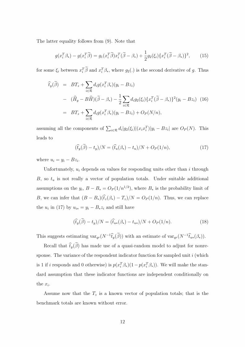
The latter equality follows from (9). Note that

g(xTi β∗)− g(xT

i β) = g1(xTi β)xT

i (β − β∗) +1

2g2(ξi){xT

i (β − β∗)}2, (15)

for some ξi between xTi β and xT

i β∗, where g2(.) is the second derivative of g. Thus

ty(β) = BTz +∑i∈R

dig(xTi β∗)(yi −Bzi)

− (Hy −BH)(β − β∗)−1

2

∑i∈R

dig2(ξi){xTi (β − β∗)}2(yi −Bzi) (16)

= BTz +∑i∈R

dig(xTi β∗)(yi −Bzi) + OP (N/n),

assuming all the components of∑

i∈R di|g2(ξi)|(xixTi )|yi −Bzi| are OP (N). This

leads to

(ty(β)− ty)/N = (tu(β∗)− tu)/N + OP (1/n), (17)

where ui = yi −Bzi.

Unfortunately, ui depends on values for responding units other than i through

B, so tu is not really a vector of population totals. Under suitable additional

assumptions on the yi, B −B∗ = OP (1/n1/2), where B∗ is the probability limit of

B, we can infer that (B − B∗)(tz(β∗) − Tz)/N = OP (1/n). Thus, we can replace

the ui in (17) by ui∗ = yi −B∗zi and still have

(ty(β)− ty)/N = (tu∗(β∗)− tu∗)/N + OP (1/n). (18)

This suggests estimating varqr(N−1ty(β)) with an estimate of varqr(N

−1tu∗(β∗)).

Recall that ty(β) has made use of a quasi-random model to adjust for nonre-

sponse. The variance of the respondent indicator function for sampled unit i (which

is 1 if i responds and 0 otherwise) is p(xTi β∗)(1−p(xT

i β∗)). We will make the stan-

dard assumption that these indicator functions are independent conditionally on

the xi.

Assume now that the Tz is a known vector of population totals; that is the

benchmark totals are known without error.

12

The component of the randomization variance of ty(β) due to nonresponse can

be estimated by

varadd =∑i∈R

d2i

p(xTi β)2

(1− p(xTi β))(yi −Bzi)(yi −Bzi)

T . (19)

Note that the right hand side of (19) does not have a component that accounts for

the uncertainty in estimating β∗ because the terms involving β − β∗ in equation

(16) are asymptotically ignorable.

When the original sample is drawn randomly without replacement, a reasonable

estimator for the (quasi-randomization) variance of ty(β) can be computed using

the right hand side of (5) with pi set to p(xTi β) and zi replaced by ui. That is to

say,

var(ty(β)) =∑i,j∈R

πij − πiπj

πijπiπjpipj

uiuTj +

∑i∈R

1− pi

p2i πi

uiuTi , (20)

where pi = p(xTi β). Proving var(ty(β)) is asymptotically unbiased is not trivial

when the right hand side of of (20) has O(n2) terms. See Kim et al. (2006) for

sufficient additional restrictions on the coefficients in that situation.

Similarly when the original sample is drawn using a stratified multi-stage rou-

tine and the first stage drawn with replacement, one can compute the variance

estimator for ty under a first-stage-with-replacement design as described in Sec-

tion 4, again with pi set to p(xTi β) and ui replacing zi.

There is an additional component in the asymptotic variance of ty(β) when Tz

is not known with certainty but is estimated from an independent external source

or sources. An obvious measure for this component is

varext = Bvar(Tz)BT , (21)

where var(Tz) is an externally-provided estimate for the variance of Tz.

Finally we note that when a full minimum β is used, equation (9) can replaced

by equation (35) of Appendix 3. This implies that, to the order of approxima-

tion used here, the results of this section still apply if the partial minimum β is

everywhere replaced by β.

13

6. Example: the 2002 Census of Agriculture

We focus our attention in this section on adjusting for unit nonresponse

in the 2002 Census of Agriculture conduction by the U.S. National Agricultural

Statistics Service (NASS). The agency used a weighting-class/poststratification

approach to adjust for whole-unit nonresponse in each state (the two are the same

for a census). Simplifying slightly, sampling units receiving Census forms were

divided in mutually exclusive response groups (poststrata) based on size class as

measured by expected sales and on whether the unit had responded to an agency

survey since 1997.

We first parallel the routine actually used by NASS and reweighted respond-

ing units in a state using these five mutually exclusive groups:

• Z-Group 1: Expected 2002 sales less than $2,500;

• Z-Group 2: Expected 2002 sales between $2,500 and $9,999;

• Z-Group 3: Expected 2002 sales between $10,000 and $49,999 and previously

reported survey data from 1997 or later;

• Z-Group 4: Expected 2002 sales greater than or equal to $50,000 and reported

survey data from 1997 or later;

• Z-Group 5: Expected 2002 sales greater than or equal to $10,000 and no

reported survey data from 1997 or later.

All the units in each state data set belonged to one of these five groups. Mathe-

matically, zi = (zi1, zi2, · · · , zi5)T , where zih = 1 when i is in Z-Group h and zih = 0

otherwise.

All di = 1 because units in the list frame were sent Census forms. The

poststatification weight for responding unit i is ci = ai = Nh/rh when the unit is

in Z-Group h, where Nh is the number of sampling units in the agency list frame

in Z-group h and rh is the number of responding entities in Z-group h.

14

We contrast this poststratification with an alternative calibration using these

same five Z-group indicator variables as benchmarks variables but different model

variables. We present here results from five state, California (CA), Delaware (DE),

Illinois (IL), Louisiana (LA), and South Dakota (SD).

In the alternative calibration, we model response as a logistic function of three

calibration x-variables: an intercept, logsales the logarithm of the actual annual

sales in 2002, truncated to the range $1,000 to $100,000, and s97 an indicator

variable for whether or not the farm responded to a survey since the 1997 Census

of Agriculture. For these runs, the fitted benchmark totals tz(β) differ from the

benchmark target totals in each state. Both sets are displayed in Table 1.

The table shows how well calibration does at estimating the benchmark totals

(recall that exact equality is not expected because there are less model variables

than benchmark variables). This is a simple check on the appropriateness of the

model. Except for Illinois, most of the estimates are within two standard errors

the benchmark totals.

In the next section we perform a simulation study using this data. Our con-

clusion is that if the response model (that is, that the probability of response is

the logistic back link of a linear combination of an intercept, logsales, and s97) is

correct then calibration works well. In contrast to that Table 1 appears to show

that this response model is, in fact, unlikely to be correct in Illinois.

We now use calibration to estimate the total number of active farms. In this

context our y variable is a 0-1 variable for being an active farm. We compare

the existing NASS approach of poststratification within Z-groups with calibration

using the three-variable model (intercept, logsales and s97). The results are given

in Table 2. Standard errors are calculated using (20) with all the πi = 1, which

is equivalent to (19). For poststratification, variance estimation assuming the re-

spondent sample results from simple random sampling within poststrata produces

identical answers asymptotically and is within roundoff error in this application.

In interpreting Table 2, it is important to realize that the standard errors are

15

computed assuming the underlying model for that fit is correct. It is well known,

and simulations in the next section document, that a misspecified response model

can introduce biases that dwarf the estimated standard errors calculated in Table

2.

The poststratification standard error assumes that response probability takes

on one of five possible values. The choice of one of these five possible values depends

upon NASS assigned expected sales and participation in surveys since 1997.

The three-variable-calibration model assumes that response probability varies

continuously with actual sales given survey participation. Although this seems

reasonable and results in estimated standard error only slightly higher than those

for poststratification, we saw in Table 1 that this model is not supported by the

data. Clearly, more research on model-fitting techniques for response modelling

through calibration is needed.

7. Simulations

As discussed in the previous section, an incorrect model is a possible expla-

nation for the poor fit provided by the three-variable models evidenced in Table

1. To explore this question further, we conducted simulations. Our conclusion is

that, if the form of the response model is correct, then calibration performs just

fine.

Our approach was as follows. For each of the five states, assuming the fitted

three-variable response model is correct, response probabilities were calculated for

each of the respondents to the Census. Then a synthetic state was created using

only the respondents to the Census, together with their response probabilities. In

particular, new target benchmarks were calculated as sizes of the Z-groups within

the synthetic state populations, that is the respondents within the original states.

Each Monte Carlo replication consisted of creating respondents within the syn-

thetic states using the assigned response probabilities and fitting a calibration

16

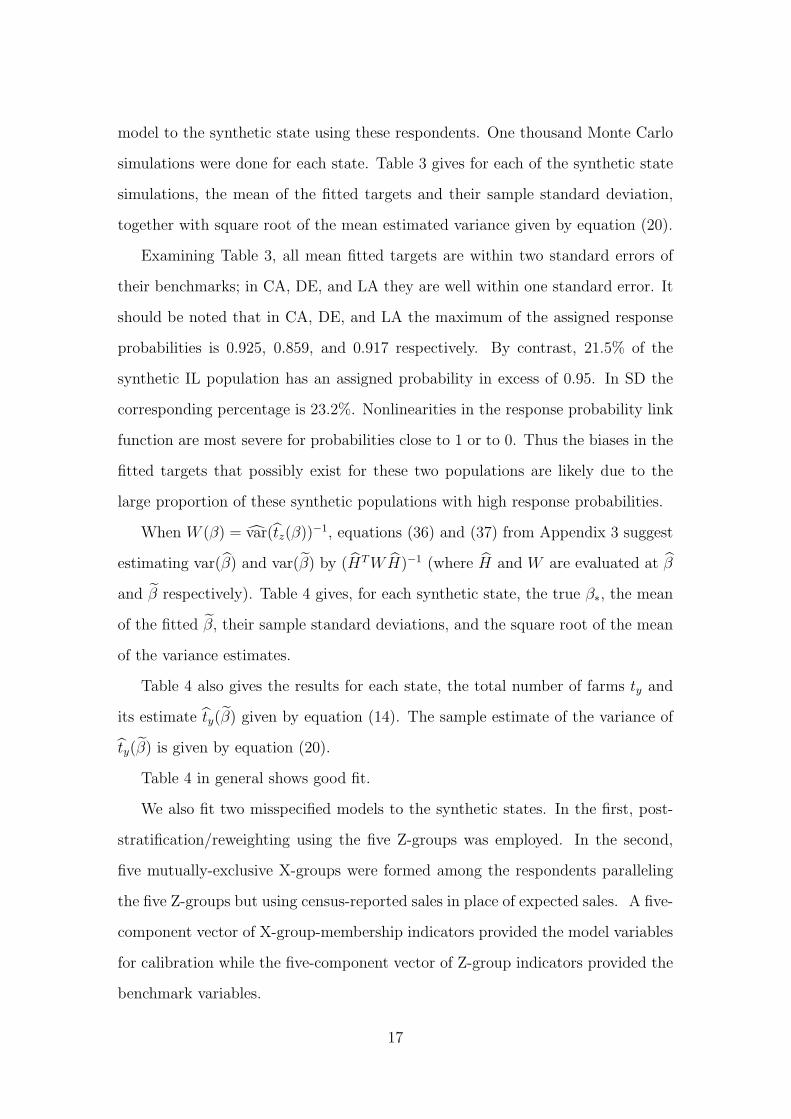
model to the synthetic state using these respondents. One thousand Monte Carlo

simulations were done for each state. Table 3 gives for each of the synthetic state

simulations, the mean of the fitted targets and their sample standard deviation,

together with square root of the mean estimated variance given by equation (20).

Examining Table 3, all mean fitted targets are within two standard errors of

their benchmarks; in CA, DE, and LA they are well within one standard error. It

should be noted that in CA, DE, and LA the maximum of the assigned response

probabilities is 0.925, 0.859, and 0.917 respectively. By contrast, 21.5% of the

synthetic IL population has an assigned probability in excess of 0.95. In SD the

corresponding percentage is 23.2%. Nonlinearities in the response probability link

function are most severe for probabilities close to 1 or to 0. Thus the biases in the

fitted targets that possibly exist for these two populations are likely due to the

large proportion of these synthetic populations with high response probabilities.

When W (β) = var(tz(β))−1, equations (36) and (37) from Appendix 3 suggest

estimating var(β) and var(β) by (HT WH)−1 (where H and W are evaluated at β

and β respectively). Table 4 gives, for each synthetic state, the true β∗, the mean

of the fitted β, their sample standard deviations, and the square root of the mean

of the variance estimates.

Table 4 also gives the results for each state, the total number of farms ty and

its estimate ty(β) given by equation (14). The sample estimate of the variance of

ty(β) is given by equation (20).

Table 4 in general shows good fit.

We also fit two misspecified models to the synthetic states. In the first, post-

stratification/reweighting using the five Z-groups was employed. In the second,

five mutually-exclusive X-groups were formed among the respondents paralleling

the five Z-groups but using census-reported sales in place of expected sales. A five-

component vector of X-group-membership indicators provided the model variables

for calibration while the five-component vector of Z-group indicators provided the

benchmark variables.

17

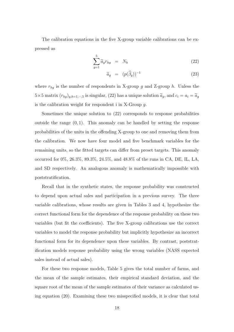
The calibration equations in the five X-group variable calibrations can be ex-

pressed as

5∑g=1

agrhg = Nh (22)

ag = (p(βg))−1 (23)

where rhg is the number of respondents in X-group g and Z-group h. Unless the

5×5 matrix (rhg)g,h=1,···,5 is singular, (22) has a unique solution ag, and ci = ai = ag

is the calibration weight for respondent i in X-Group g.

Sometimes the unique solution to (22) corresponds to response probabilities

outside the range (0, 1). This anomaly can be handled by setting the response

probabilities of the units in the offending X-group to one and removing them from

the calibration. We now have four model and five benchmark variables for the

remaining units, so the fitted targets can differ from preset targets. This anomaly

occurred for 0%, 26.3%, 89.3%, 24.5%, and 48.8% of the runs in CA, DE, IL, LA,

and SD respectively. An analogous anomaly is mathematically impossible with

poststratification.

Recall that in the synthetic states, the response probability was constructed

to depend upon actual sales and participation in a previous survey. The three

variable calibrations, whose results are given in Tables 3 and 4, hypothesize the

correct functional form for the dependence of the response probability on these two

variables (but fit the coefficients). The five X-group calibrations use the correct

variables to model the response probability but implicitly hypothesize an incorrect

functional form for its dependence upon these variables. By contrast, poststrat-

ification models response probability using the wrong variables (NASS expected

sales instead of actual sales).

For these two response models, Table 5 gives the total number of farms, and

the mean of the sample estimates, their empirical standard deviation, and the

square root of the mean of the sample estimates of their variance as calculated us-

ing equation (20). Examining these two misspecified models, it is clear that total

18

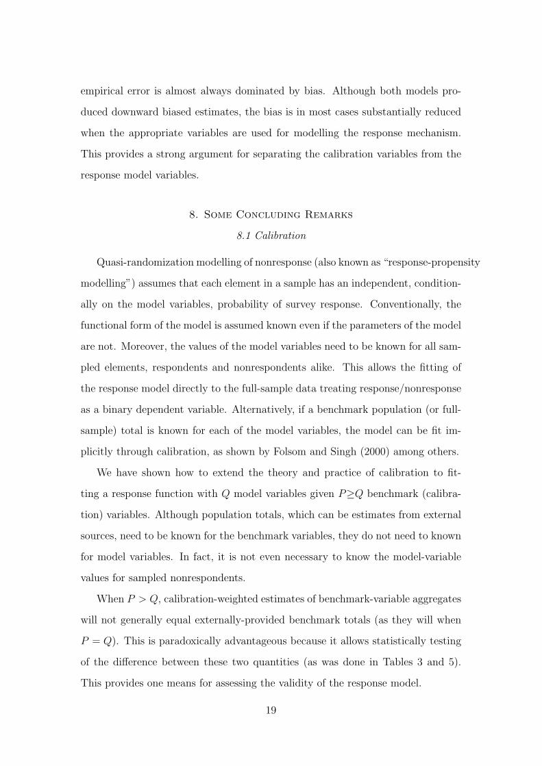
empirical error is almost always dominated by bias. Although both models pro-

duced downward biased estimates, the bias is in most cases substantially reduced

when the appropriate variables are used for modelling the response mechanism.

This provides a strong argument for separating the calibration variables from the

response model variables.

8. Some Concluding Remarks

8.1 Calibration

Quasi-randomization modelling of nonresponse (also known as “response-propensity

modelling”) assumes that each element in a sample has an independent, condition-

ally on the model variables, probability of survey response. Conventionally, the

functional form of the model is assumed known even if the parameters of the model

are not. Moreover, the values of the model variables need to be known for all sam-

pled elements, respondents and nonrespondents alike. This allows the fitting of

the response model directly to the full-sample data treating response/nonresponse

as a binary dependent variable. Alternatively, if a benchmark population (or full-

sample) total is known for each of the model variables, the model can be fit im-

plicitly through calibration, as shown by Folsom and Singh (2000) among others.

We have shown how to extend the theory and practice of calibration to fit-

ting a response function with Q model variables given P≥Q benchmark (calibra-

tion) variables. Although population totals, which can be estimates from external

sources, need to be known for the benchmark variables, they do not need to known

for model variables. In fact, it is not even necessary to know the model-variable

values for sampled nonrespondents.

When P > Q, calibration-weighted estimates of benchmark-variable aggregates

will not generally equal externally-provided benchmark totals (as they will when

P = Q). This is paradoxically advantageous because it allows statistically testing

of the difference between these two quantities (as was done in Tables 3 and 5).

This provides one means for assessing the validity of the response model.

19

8.2 Partial minimization

The appendices establish conditions for the existence of both a full minimum to

the objective function (equation (4)) or a partial minimum solution to (9), at least

given a large-enough sample. These solutions both serve as consistent estimators

for the response-model parameter. In our own empirical investigations, we found

it much simpler to reach an iterative “partial-minimization” solution to equation

(9). The two solutions were generally close. We recommend statisticians use the

partial-minimization approach in practice.

The two approaches differ only when the matrix W is itself a function of β, for

example, when it is be the inverse of the variance of tz(β). We found in simulations

(not shown) that using the identity matrix in place of W in (9) decreased the

efficiency of the resulting estimates when derived under the correct response model.

Nevertheless, these estimates were consistent, as our theory anticipated.

By setting W equal to the inverse of a quasi-randomization with-replacement

variance estimator for tz(β) in Appendix 2, we established sufficient conditions for

the existence of a minimum of the objective function given a large-enough sample.

In practice, we recommend using the without-replacement variance estimator in

this context when practical (e.g., for single-stage original samples with known joint

selection probabilities). Recomputing W assuming a with-replacement original

sample and n = N in our simulations did not appreciably change the results for

the estimators or their variances.

8.3 Coverage error

It is a simple matter to adapt most of the results in this paper to the situation

where calibration is used to adjust for coverage errors, whether from frame under-

coverage or unit duplication. In this context, pi is the expected number of times

population unit i is in the frame. Under the assumed quasi-randomization model

20

this value is independent of the actual sample drawn and of how many times other

elements of the population are in the frame.

The possibility a unit appearing more than once on a frame does cause some

small differences in variance estimation. When there is no possibility of unit du-

plication, the variance of the function indicating whether population unit i is in

the frame is p(xTi β∗)(1− p(xT

i β∗)), paralleling the situation with survey response.

When the frame contains potential duplication, however, the variance of the ex-

pected number of times a population unit is no longer p(xTi β∗)(1− p(xT

i β∗)). Con-

sequently, its value will need to be assumed for the analogue of (19), a measure of

the added variance due to frame errors, to be derived.

When using calibration to adjust for coverage errors, it is likely that the com-

ponents of Tz will be estimates coming from external sources. If the (internal)

sample size is fairly large, it may be reasonable to set W = (var(Tz))−1, where

var(Tz) is externally provided.

8.4 Final remarks

Returning to response modelling, although the following applies equally well

to coverage modelling, much work is needed in determining how to select model

and benchmark variables in practice and assessing the usefulness of an asymp-

totic theory on finite samples. Additional complication arise when the targets of

the benchmark variables are themselves potentially subject to sampling and mea-

surement errors. Nevertheless, by allowing a separation between the model and

benchmark variables, the approach to calibration developed here may open the

door to more plausible modelling of the response mechanism.

Avoiding response and coverage modelling as much as possible remains a pru-

dent policy. Even the cleverest model assumptions are difficult to test and prone to

failure. Unfortunately, eschewing models will not be viable option as surveys based

on incomplete frames or suffering from small response rates become increasingly

common.

21

Acknowledgements

The authors wish to thank the referees for their close reading of the manuscript

and many thoughtful suggestions.

Appendix 1

Proof of variance formula (5)

Let tz denote tz(β∗). Then

var(tz) = var(E(tz|S)) + E(var(tz|S))

Using Sarndal et al. (1992) Result 9.3.1

var(E(tz|S)) =∑i,j∈U

πij − πiπj

πiπj

zizTj

E(var(tz|S)) =∑i∈U

1− pi

piπi

zizTi .

and the sample estimates of these variance components are

var(E(tz|S)) =∑

i6=j∈R

πij − πiπj

πijπiπjpipj

zizTj +

∑i∈R

1− πi

π2i pi

zizTi

E(var(tz|S)) =∑i∈R

1− pi

p2i π

2i

zizTi .

Combining these two yields equation (5). 2

Appendix 2

Quasi-randomization consistency of the full minimum β

The estimate β minimizes the slightly redefined objective function

n−1ρ(β) = −n−1logdet(N2

nW (β)) (24)

+(N−1Tz −N−1tz(β)

)T (N2

nW (β)

)(N−1Tz −N−1tz(β)

)

22

where n denotes the sample size before nonresponse, N the population size, and

Tz the vector of calibration targets. Now

tz(β) =∑i∈R

di

p(xTi β)

zi (25)

has expected value under the quasi-randomization model

tz(β) =∑i∈U

p(xTi β∗)

p(xTi β)

zi. (26)

Conditionally on S, the expected value of tz(β) is

tzS(β) = E(tz(β)|S) =∑i∈S

π−1i

p(xTi β∗)

p(xTi β)

zi. (27)

Assumption 1 We assume that xi and β are constrained to lie in compact sets

and that these compact sets are such that p(xT β) is bounded away from 0.

Assumption 2 The limits lim N−1tz(β) and lim N−1Tz converge, with the former

limit converging uniformly in β. These limits satisfy

lim N−1tz(β∗) = lim N−1Tz

lim N−1tz(β) 6= lim N−1Tz

for β 6= β∗.

Let

ρ0(β) = (lim N−1Tz − lim N−1tz(β))T W0(β)(lim N−1Tz − lim N−1tz(β)),

where W0(β) is a positive definite symmetric matrix to be specified shortly.

If Assumption 2 is true, then ρ0(β) is uniquely minimized at β = β∗. Wald’s

proof of the consistency of the maximum likelihood estimate (see, for example,

Silvey (1975)) can be used to show the consistency of β if it can be established

that

n−1ρ(β) →P ρ0(β)

23

uniformly in β. In other words, we need to establish that, uniformly in β,

N−1tz(β)−N−1tz(β) →P 0

N2

nW (β) →P W0(β), (28)

where →P refers to convergence in probability with respect to both the sampling

design and the response model.

Wald’s proof establishes that for large enough samples, the minimum β to

equation (24) exists.

A formal asymptotic structure must postulate a sequence of populations and

sampling designs, indexed in what follows by r, so that the population size Nr can

grow along with the sample size nr. Several examples of such asymptotic structure

can be found in Fuller and Isaki (1981). This paper can be applied to many

useful fixed sample size without replacement designs. Lemma 1 of Fuller and Isaki

(1981) would apply, for example, if the sampling design is a stratified two stage

cluster sample in which the number of strata is fixed (in r), the number of PSUs

in each stratum increases as r →∞, the first stage sampling fraction within each

stratum of PSU’s is bounded away from 0 and 1, and the second stage sampling

fractions are bounded away from 0. We will establish consistency of β within this

asymptotic framework, using Fuller and Isaki type assumptions on the original

sampling scheme. Although not all designs of interest can be accommodated within

this asymptotic framework, we offer these proofs to illustrate the reasoning that

might apply elsewhere.

Let the inclusion probabilities for the r-th universe and design be denoted by

πi(r) and πij(r), so that di = π−1i(r). We require that the original element sample size

nr be fixed, but the respondent sample size is random. Assumption 3 is a special

case of the assumptions in Fuller and Isaki’s Lemma 1.

Assumption 3 Assume that for all r and all i 6= j

πi(r)πj(r) − πij(r) ≤ αn−1r πi(r)πj(r)

24

N−2r nr

∑i∈Ur

πi(r)

[π−1

i(r)zi − n−1r tz(r)(β∗)

] [π−1

i(r)zi − n−1r tz(r)(β∗)

]T� M2

where α is a fixed constant, M2 a fixed positive definite symmetric matrix, tz(r)(β) is

defined using equation (26) from the r-th universe Ur, and, for symmetric matrices

A and B, A � B means B − A is positive semi-definite.

Proposition 1 Under assumptions 1, 2, and 3,

N−1tz(β)−N−1tz(β) = OP (n−.5)

uniformly in β.

Proof: For notational simplicity, we drop the index r in this proof. Let ui =

p(xTi β)−1p(xT

i β∗)zi. Using Assumption 1, p(xTi β)−1p(xT

i β∗) < C for all β and all

xi. Thus since n =∑

i∈U πi,

N−2n∑i∈U

πi

{π−1

i ui − n−1tz(β)}{

π−1i ui − n−1tz(β)

}T

= N−2n∑i∈U

π−1i uiu

Ti −N−2tz(β)tz(β)T

� C2N−2n∑i∈U

π−1i ziz

Ti

� C2{M2 + N−2tz(β∗)tz(β∗)

T}

.

Examining the proof of Lemma 1 in Fuller and Isaki (1981), it follows that N−1tzS(β)−

N−1tz(β) is OP (n−.5), uniformly in β.

Notice also that the above establishes that N−2∑

i∈U π−1i ziz

Ti is O(n−1). Let

T = N−1tz(β)−N−1tzS(β). Then E(T |S) = 0 and

var(T |S) = N−2∑i∈S

π−2i

p(xTi β∗)− p(xT

i β∗)2

p(xTi β)2

zizTi

E[var(T |S)] = N−2∑i∈U

π−1i

p(xTi β∗)− p(xT

i β∗)2

p(xTi β)2

zizTi ,

which is O(n−1), uniformly in β. Thus T = OP (n−.5), uniformly in β which

establishes the Proposition. 2

25

We now turn to establishing (28), that is N2n−1W (β) →P W0(β), where W0(β)

is positive definite symmetric. First of all we note that W (β) can be scaled by a

constant without changing β. Thus if cNW (β) converges uniformly to a positive

definite symmetric matrix, we can redefine W (β) so that (28) holds. Thus, for

example, if W (β) = var(Tz)−1 and var(Tz) is externally defined, one has to assume

the existence of a cN which makes (28) true.

Here we will show that if W (β) is the inverse of a with replacement estimated

covariance matrix, then (28) will often hold (under the original design).

Proposition 2 If an element sample S is drawn with replacement and expected

counts πi, then the variance varwr(tz) of tz =∑

i∈R π−1i p−1

i zi is

varwr(tz) =∑i∈U

π−1i p−1

i zizTi − n−1tzt

Tz . (29)

It can be unbiasedly estimated by

varwr(tz) =n

n− 1

∑i∈R

(π−1

i p−1i zi − n−1tz

) (π−1

i p−1i zi − n−1tz

)T(30)

Proof: Since E(tz|S) =∑

i∈S π−1i zi, Sarndal et al. (1992) formulas (3.6.14) and

(3.5.5) yield

var(E(tz|S)) =∑i∈U

πi

(π−1

i zi − n−1tz) (

π−1i zi − n−1tz

)TE(var(tz|S)) =

∑i∈U

1− pi

πipi

zizTi .

These two sum to the expression in (29). Now

E(varwr(tz)) =n

n− 1E(∑i∈R

zizTi

π2i p

2i

− n−1tz tTz )

=n

n− 1

[∑i∈U

zizTi

πipi

− n−1{varwr(tz) + tzt

Tz

}]which yields (29) with some algebra. 2

Remark: Recall our intention is to use equation (30) to define a suitable W (β)

for estimating β with a nonreplacement sample. Consequently we felt free to

26

take certain liberties in the statement of Proposition 2. Formally, we require

that S = (j1, ..., jn) is an ordered sample with Pr[jk = i] = n−1πi for all k =

1, . . . , n and that R is an ordered Poisson subsample with Pr[jk ∈ R] = pjk. In

particular it is assumed that the events jk ∈ R and jl ∈ R are independent,

conditionally on S. Although this independence assumption is dubious when jk =

jl in the interpretation of R as respondent set, this contingency does not arise in

a nonreplacement sample.

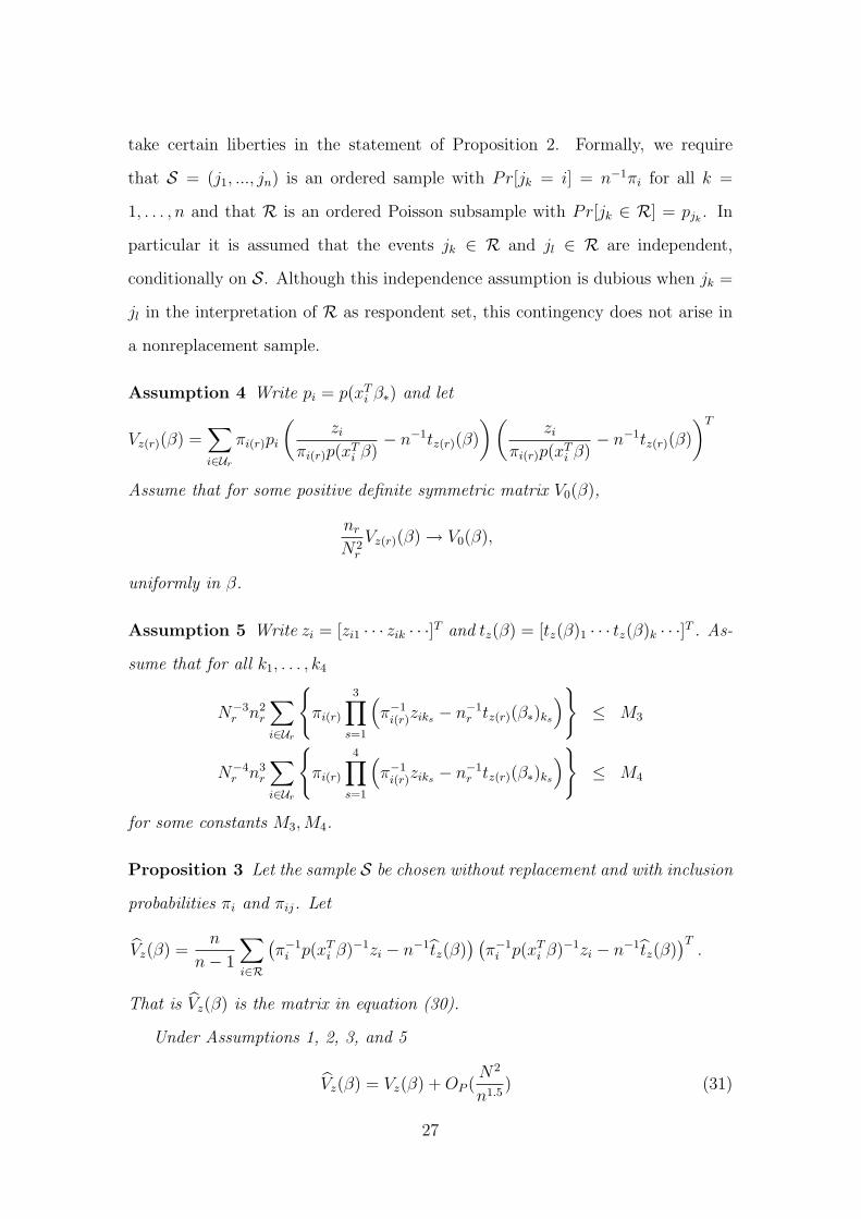
Assumption 4 Write pi = p(xTi β∗) and let

Vz(r)(β) =∑i∈Ur

πi(r)pi

(zi

πi(r)p(xTi β)

− n−1tz(r)(β)

)(zi

πi(r)p(xTi β)

− n−1tz(r)(β)

)T

Assume that for some positive definite symmetric matrix V0(β),

nr

N2r

Vz(r)(β) → V0(β),

uniformly in β.

Assumption 5 Write zi = [zi1 · · · zik · · ·]T and tz(β) = [tz(β)1 · · · tz(β)k · · ·]T . As-

sume that for all k1, . . . , k4

N−3r n2

r

∑i∈Ur

{πi(r)

3∏s=1

(π−1

i(r)ziks − n−1r tz(r)(β∗)ks

)}≤ M3

N−4r n3

r

∑i∈Ur

{πi(r)

4∏s=1

(π−1

i(r)ziks − n−1r tz(r)(β∗)ks

)}≤ M4

for some constants M3, M4.

Proposition 3 Let the sample S be chosen without replacement and with inclusion

probabilities πi and πij. Let

Vz(β) =n

n− 1

∑i∈R

(π−1

i p(xTi β)−1zi − n−1tz(β)

) (π−1

i p(xTi β)−1zi − n−1tz(β)

)T.

That is Vz(β) is the matrix in equation (30).

Under Assumptions 1, 2, 3, and 5

Vz(β) = Vz(β) + OP (N2

n1.5) (31)

27

uniformly in β. Hence, assuming in addition Assumption 4,

n

N2Vz(β) →P V0(β)

uniformly in β.

Proof: For simplicity of notation, we assume that z is univariate. In addition, as

in Proposition 1, Assumption 1 yields uniformity in β as long as we can establish

the proposition for β = β∗. Thus we will suppress the β in what follows.

Furthermore, it is easily checked that Assumptions 1, 2, 3, and 5 imply

N−4n3∑i∈U

πipi

(zi

πipi

− n−1tz

)4

≤ M0

for some constant M0.

With a little algebra and using Proposition 1

Vz =(1 + O(n−1)

){∑i∈R

(zi

πipi

− n−1tz)2 − n−1(tz − tz)

2

}

=(1 + O(n−1)

){∑i∈R

(zi

πipi

− n−1tz)2 + OP (N2/n2)

}.

Let

Vz =∑i∈R

(zi

πipi

− n−1tz)2. (32)

Now

E(Vz) =∑i∈U

πipi(zi

πipi

− n−1tz)2 = Vz

which can be shown to be O(N2/n) using Assumptions 1 and 3.

Furthermore

E(Vz|S) =∑i∈S

pi(zi

πipi

− n−1tz)2

var(E(Vz|S)) =−1

2

∑i,j∈U

(πij − πiπj)

{pi(

zi

πipi

− n−1tz)2 − pj(

zj

πjpj

− n−1tz)2

}2

≤ α

n

∑i,j∈U

πiπj

{p2

i (zi

πipi

− n−1tz)4 − pipj(

zi

πipi

− n−1tz)2(

zj

πjpj

− n−1tz)2

}

28

= α∑i∈U

πip2i (

zi

πipi

− n−1tz)4 − α

nV 2

z = O(N4/n3)

var(Vz|S) =∑i∈S

(pi − p2i )(

zi

πipi

− n−1tz)4

E(var(Vz|S)) =∑i∈U

πi(pi − p2i )(

zi

πipi

− n−1tz)4 = O(N4/n3),

where we have applied Assumption 5 and noted that p2i < pi. Equation (31)

follows. 2

Appendix 3

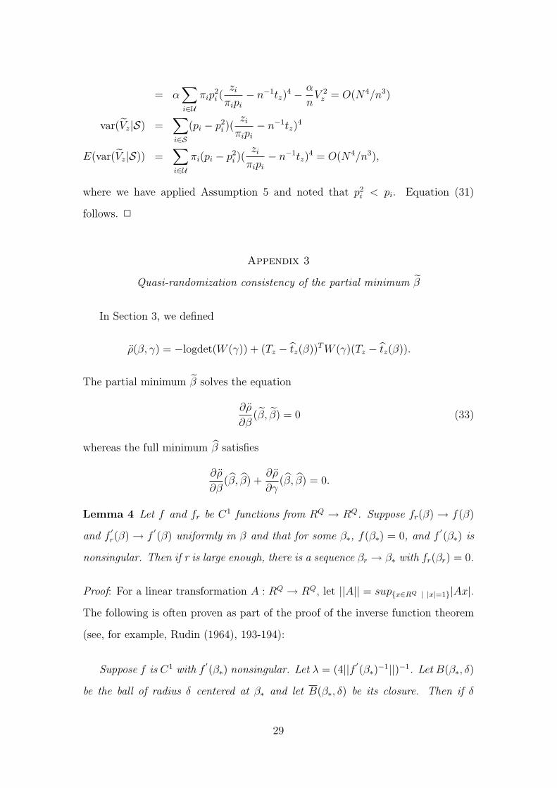
Quasi-randomization consistency of the partial minimum β

In Section 3, we defined

ρ(β, γ) = −logdet(W (γ)) + (Tz − tz(β))T W (γ)(Tz − tz(β)).

The partial minimum β solves the equation

∂ρ

∂β(β, β) = 0 (33)

whereas the full minimum β satisfies

∂ρ

∂β(β, β) +

∂ρ

∂γ(β, β) = 0.

Lemma 4 Let f and fr be C1 functions from RQ → RQ. Suppose fr(β) → f(β)

and f′r(β) → f

′(β) uniformly in β and that for some β∗, f(β∗) = 0, and f

′(β∗) is

nonsingular. Then if r is large enough, there is a sequence βr → β∗ with fr(βr) = 0.

Proof: For a linear transformation A : RQ → RQ, let ||A|| = sup{x∈RQ | |x|=1}|Ax|.

The following is often proven as part of the proof of the inverse function theorem

(see, for example, Rudin (1964), 193-194):

Suppose f is C1 with f′(β∗) nonsingular. Let λ = (4||f ′

(β∗)−1||)−1. Let B(β∗, δ)

be the ball of radius δ centered at β∗ and let B(β∗, δ) be its closure. Then if δ

29

is sufficiently small so that ||f ′(β) − f

′(β∗)|| < 2λ for all β ∈ B(β∗, δ), then

f(B(β∗, δ)) contains B(f(β∗), λδ).

Pick a compact neighborhood C of β∗ that is in the domain of all the fr and

f . Pick N so that ||f ′r(β∗)

−1 − f′(β∗)

−1|| ≤ 12||f ′

(β∗)−1|| for all r > N . Then

23λ ≤ λr = (4||f ′

r(β∗)−1||)−1.

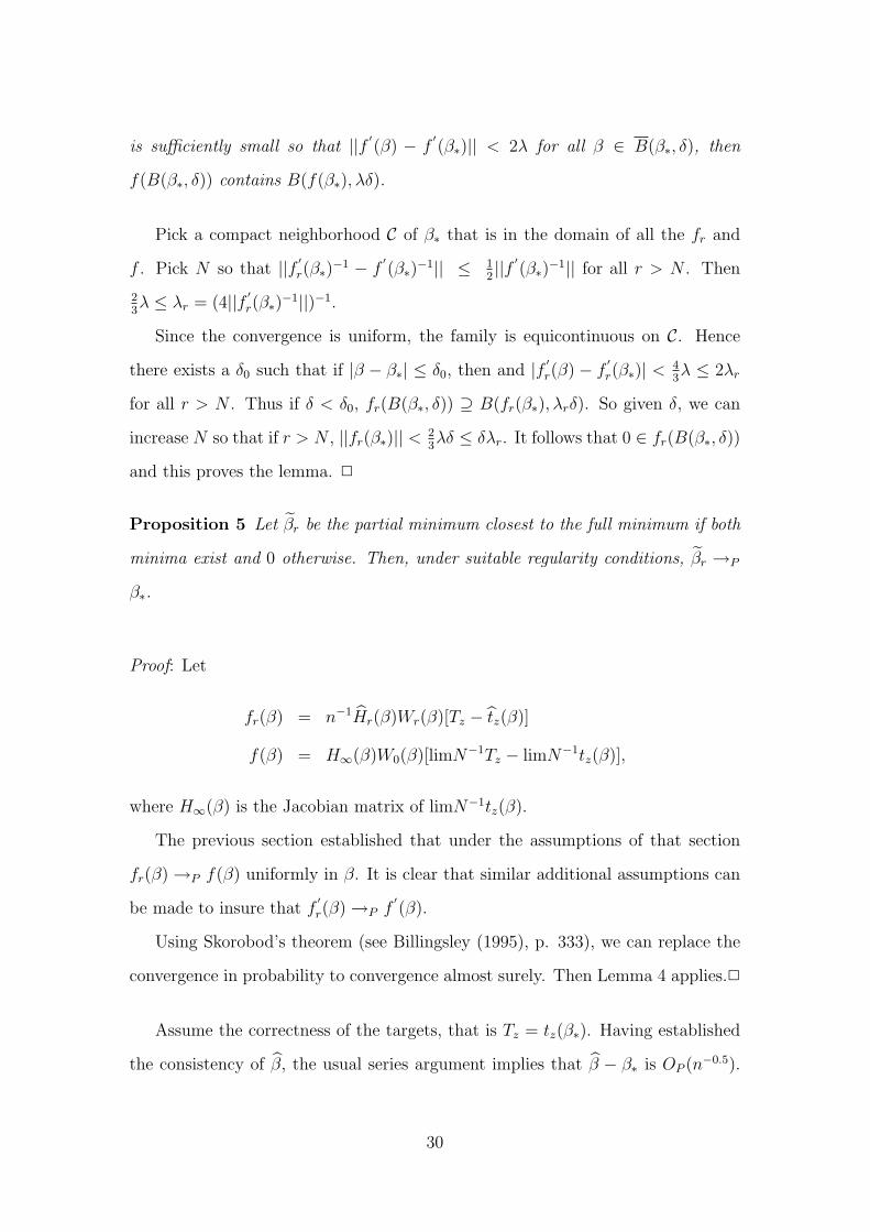
Since the convergence is uniform, the family is equicontinuous on C. Hence

there exists a δ0 such that if |β − β∗| ≤ δ0, then and |f ′r(β) − f

′r(β∗)| < 4

3λ ≤ 2λr

for all r > N . Thus if δ < δ0, fr(B(β∗, δ)) ⊇ B(fr(β∗), λrδ). So given δ, we can

increase N so that if r > N , ||fr(β∗)|| < 23λδ ≤ δλr. It follows that 0 ∈ fr(B(β∗, δ))

and this proves the lemma. 2

Proposition 5 Let βr be the partial minimum closest to the full minimum if both

minima exist and 0 otherwise. Then, under suitable regularity conditions, βr →P

β∗.

Proof: Let

fr(β) = n−1Hr(β)Wr(β)[Tz − tz(β)]

f(β) = H∞(β)W0(β)[limN−1Tz − limN−1tz(β)],

where H∞(β) is the Jacobian matrix of limN−1tz(β).

The previous section established that under the assumptions of that section

fr(β) →P f(β) uniformly in β. It is clear that similar additional assumptions can

be made to insure that f′r(β) →P f

′(β).

Using Skorobod’s theorem (see Billingsley (1995), p. 333), we can replace the

convergence in probability to convergence almost surely. Then Lemma 4 applies.2

Assume the correctness of the targets, that is Tz = tz(β∗). Having established

the consistency of β, the usual series argument implies that β − β∗ is OP (n−0.5).

30

Thus

n−1ρ′(β) = −n−1 d logdetN2

nW (β)

dβ

− 2N−1

(dtz(β)

dβ

)TN2

nW (β)

(N−1Tz −N−1tz(β)

)(34)

+(N−1Tz −N−1tz(β)

)T dN2

nW (β)

dβ

(N−1Tz −N−1tz(β)

).

Since

N−1(Tz − tz(β)

)= N−1

(tz(β∗)− tz(β∗) + H(β)(β∗ − β)

)+ OP (n−1)

= OP (n−0.5),

when evaluated at β, the first and third terms of the right hand side of (34) are

OP (n−1). Hence

H(β)T W (β)(Tz − tz(β)

)= OP (1) (35)

On the other hand, the partial minimum satisfies (see equation (9))

H(β)T W (β)(Tz − tz(β)

)= OP (1)

Finally we have

β = β∗ +{

H(β)T W (β)H(β)}−1

H(β)T W (β)(Tz − tz(β∗)) + OP (n−1) (36)

β = β∗ +{

H(β)T W (β)H(β)}−1

H(β)T W (β)(Tz − tz(β∗)) + OP (n−1). (37)

References

Billingsley, P. (1995) Probability and Measure, 3rd ed., Wiley, New York.

Crouse, C. and Kott, P.S. (2004). “Evaluating Alternative Calibration

Schemes for an Economic Survey with Large Nonresponse,” ASA Proceedings

of the Survey Reseach Methods Section.

31

Folsom., R.E. (1991). Exponential and Logistic Weight Adjustment for Sam-

pling and Nonresponse Error Reduction, ASA Proceedings of the Social Statis-

tics Section, 197-202.

Folsom., R.E. and Singh, A.C. (2000). The Generalized Exponential Model

for Sampling Weight Calibration for Extreme Values, Nonresponse, and Post-

stratification, ASA Proceedings of the Section on Survey Research Methods,

598-603.

Fuller, W.A. and Isaki, C.T. (1981). Survey Design Under Superpopulation

Models in Current Topics in Survey Sampling, eds. D. Krewshi, J.N.K. Rao,

and R. Platek, New York: Academic Press.

Fuller, W.A., Loughin, M.M., and Baker, H.D. (1994). Regression

Weighting for the 1987-88 National Food Consumption Survey, Survey Method-

ology 20, 75-85.

Kim, J.K., Navarro, A., and Fuller, W.A. (2006). Replicate Variance Es-

timation for Two-Phase Stratified Sampling, J. Am. Statist. Assoc., forth-

coming.

Kish, L. (1965). Survey Sampling, Wiley, New York.

Kott, P.S. (2006). Using Calibration Weighting to Adjust for Nonresponse and

Coverage Errors, Survey Methodology 32, 133-42.

Lohr, S. L. (1999). Sampling Design and Analysis, Pacific Grove, CA: Duxbury

Press.

Lundstrom, S. and Sarndal, C.-E. (1999). Calibration as a Standard

Method for the Treatment of Nonresponse, J. Official Statist. 15, 305-327.

McCullagh, P. and Nelder, J.A. (1989). Generalized Linear Models, Second

edition, London: Chapman & Hall.

32

Rudin, W. (1964). Principles of Mathematical Analysis, 2nd ed., McGraw-Hill,

New York.

Sarndal, C.-E. and Lundstrom, S. (2005). Estimation in Surveys with

Nonresponse, New York: Wiley.

Sarndal, C.-E., Swensson, B., and Wretman, J. (1992). Model Assisted

Survey Sampling, New York: Springer-Verlag.

Silvey, J. D. (1975). Statistical Inference, London: Chapman & Hall.

Thompson, M. E. (1997). Theory of Sample Surveys, London: Chapman &

Hall.

33

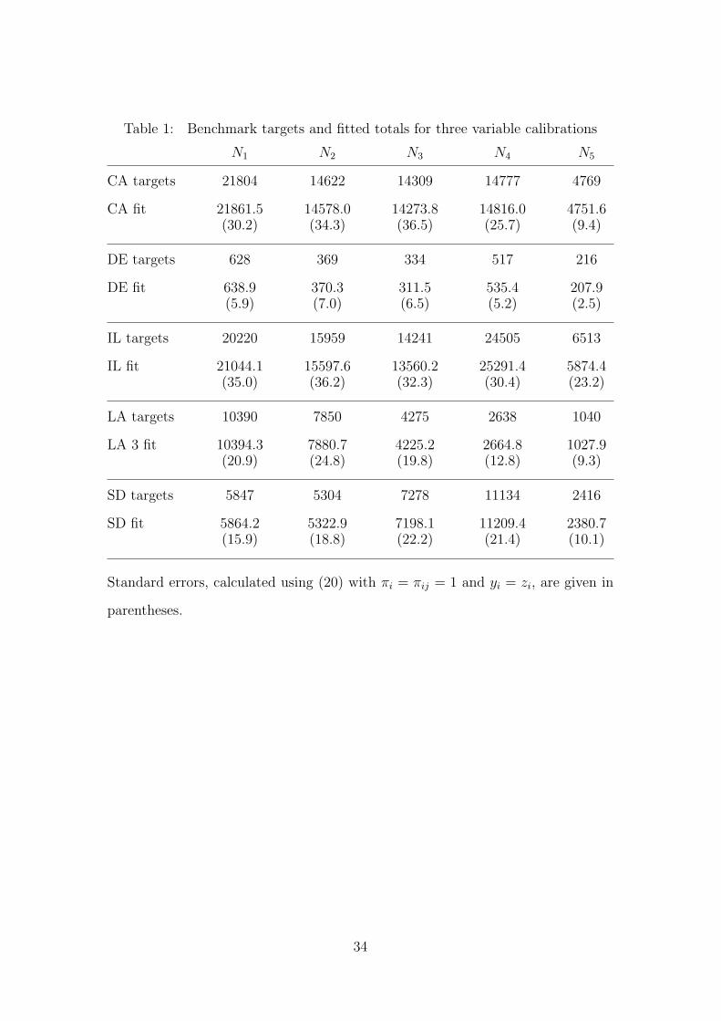
Table 1: Benchmark targets and fitted totals for three variable calibrations

N1 N2 N3 N4 N5

CA targets 21804 14622 14309 14777 4769

CA fit 21861.5 14578.0 14273.8 14816.0 4751.6(30.2) (34.3) (36.5) (25.7) (9.4)

DE targets 628 369 334 517 216

DE fit 638.9 370.3 311.5 535.4 207.9(5.9) (7.0) (6.5) (5.2) (2.5)

IL targets 20220 15959 14241 24505 6513

IL fit 21044.1 15597.6 13560.2 25291.4 5874.4(35.0) (36.2) (32.3) (30.4) (23.2)

LA targets 10390 7850 4275 2638 1040

LA 3 fit 10394.3 7880.7 4225.2 2664.8 1027.9(20.9) (24.8) (19.8) (12.8) (9.3)

SD targets 5847 5304 7278 11134 2416

SD fit 5864.2 5322.9 7198.1 11209.4 2380.7(15.9) (18.8) (22.2) (21.4) (10.1)

Standard errors, calculated using (20) with πi = πij = 1 and yi = zi, are given in

parentheses.

34

Table 2: Estimated number of farms

poststratification using calibration using5 Z-groups intercept, logsales, s97

CA 45312.5 (45.8) 46178.8 (56.3)

DE 1390.9 (9.2) 1400.6 (11.0)

IL 57332.4 (52.1) 58925.7 (53.7)

LA 16139.6 (30.3) 16425.3 (37.6)

SD 23260.7 (27.7) 23821.1 (25.5)

Standard errors in parentheses.

35

Table 3: Benchmark targets and fitted totals for three model variable calibrations,

simulated populations

N1 N2 N3 N4 N5

CA targets 19603 13034 12502 12463 3967

CA fitted 19603.28 13033.60 12502.34 12462.83 3966.9628.11 32.42 34.01 23.26 8.6428.42 32.16 33.75 23.37 8.75

DE targets 537 311 259 435 167

DE fitted 537.02 310.99 259.04 434.96 166.995.39 6.40 6.04 4.75 2.315.42 6.42 5.96 4.73 2.30

L targets 18542 14000 12048 20268 4388

IL fitted 18540.11 14001.55 12048.90 20266.67 4388.9131.11 31.97 27.91 25.51 20.4430.88 32.39 28.72 25.91 20.55

LA targets 9054 6938 3673 2182 806

LA fitted 9054.15 6938.15 3672.75 2182.09 805.8719.64 22.65 18.39 11.37 8.6419.30 22.61 18.24 11.14 8.45

SD targets 5358 4876 6499 9378 1837

SD fitted 5357.63 4876.97 6498.43 9378.30 1836.6614.57 17.52 20.22 19.24 9.3414.37 17.23 20.01 19.06 9.23

Based upon 1000 simulations. For each fitted model, the first line gives the mean

of the fitted targets, the second their empirical standard deviations, and the third

the square root of the mean of the sample estimated variances calculated using

(20).

36

Table 4: Coefficients β∗ and total number of farms ty, together with estimates β

and ty(β), three model variable calibrations on simulated populations

Coefficients

int logsales s97 Number of Farms

CA β∗ and ty 3.7478 -0.2341 0.3841 39568

CA fitted β and ty(β) 3.7433 -0.2335 0.3835 39565.530.1051 0.0132 0.0510 52.810.1062 0.0132 0.0507 53.57

DE β∗ and ty 2.3161 -0.0964 0.1543 1147

DE fitted β and ty(β) 2.3292 -0.0957 0.1379 1146.610.4934 0.0638 0.2227 10.630.4908 0.0628 0.2230 10.16

IL β∗ and ty 5.2025 -0.4548 1.1894 48608

IL fitted β and ty(β) 5.2009 -0.4545 1.1886 48605.320.1193 0.0152 0.0525 48.590.1207 0.0154 0.0540 48.30

LA β∗ and ty 3.5327 -0.2617 0.6822 13944

LA fitted β and ty(β) 3.5277 -0.2609 0.6813 13944.630.1899 0.0269 0.0958 35.560.1898 0.0269 0.0952 35.21

SD β∗ and ty 6.0846 -0.5188 1.2285 20231

SD fitted β and ty(β) 6.0915 -0.5193 1.2281 20230.130.2287 0.0272 0.0846 24.200.2316 0.0276 0.0856 23.95

Based upon 1000 simulations. These calibrations fit a correct model. For each

state, the first line contains the true values, the second contains the mean of the

fitted values, the third their empirical standard deviations, and the fourth the

square root of the mean of the estimated variances.

37

Table 5: Estimated number of farms, simulated populations

Poststratification: 5 Z-groups Calibration: 4/5 X-variables

standard error standard error

No. farms mean empirical eqn (20) mean empirical eqn (20)

CA 39568 38815.03 39.62 42.86 39365.00 154.60 156.68

DE 1147 1138.96 8.01 8.41 1145.66 15.97 16.91

IL 48608 47369.47 37.58 45.38 48133.22 73.04 79.66

LA 13944 13708.36 26.03 27.92 13713.93 81.04 91.46

SD 20231 19766.06 19.51 25.17 20081.41 43.86 51.50

Based upon 1000 simulations. Both of these calibrations fit incorrect models.

Poststratification fits the wrong model variables; the calibration model fits the

correct model variables with the wrong functional form. Notice that although

both models have estimates that appear to be biased downward, the bias is worse

for the model with the incorrect model variables and that this bias is much more

important than the standard error of the estimates.

38