using the acs to implement a supplemental poverty measure (spm)
TRANSCRIPT
1
Using the American Community Survey (ACS) to Implement a Supplemental Poverty Measure (SPM) 1
Trudi Renwick
Social, Economic and Housing Statistics Division U.S. Census Bureau
Working Paper # 2015-09
June 2015
Introduction
In 2009, the Office of Management and Budget’s Chief Statistician formed an
Interagency Technical Working Group (ITWG) that issued a series of suggestions to the
Census Bureau and the Bureau of Labor Statistics on how to develop a new Supplemental
Poverty Measure (SPM).2 Their suggestions drew on the recommendations of the 1995
report of the National Academy of Sciences (NAS) Panel on Poverty and Family
Assistance and the extensive research on poverty measurement conducted over the past
15 years at the Census Bureau and elsewhere. The ITWG suggestions focused on the
implementation of the new measure using the Current Population Survey Annual Social
and Economic Supplement (CPS ASEC). The ITWG stated that the SPM will not replace
the official poverty measure and will not be used to define program eligibility. The
Census Bureau released preliminary research SPM estimates in November 2011, 2012
and 2013 (Short 2011, Short 2012, Short 2013).
1 Paper originally presented at the November 2014 Fall Research Conference of the Association for Public Policy Analysis and Management, Albuquerque, NM. This paper reports the results of research and analysis undertaken by Census Bureau staff. It has undergone more limited review than official publications. Any views expressed on statistical, methodological, technical, or operational issues are those of the authors and not necessarily those of the U.S. Census Bureau. Estimates revised May 2015. 2 Observations from the Interagency Technical Working Group on Developing a Supplemental Poverty Measure. March 2010, http://www.census.gov/hhes/www/poverty/SPM_TWGObservations.pdf
2
The Census Bureau releases official poverty estimates each year using the CPS
ASEC. Poverty estimates calculated using the official definition can be created relatively
easily in other surveys. For official poverty estimates for state and sub-state geographic
units, the Census Bureau recommends the use of the American Community Survey
(ACS).
The research SPM estimates released for the past three years uses the CPS ASEC.
Unlike the official definition, the SPM is not as easily calculated in other surveys.
Therefore, on April 1, 2011, the Census Bureau sponsored a workshop at the Urban
Institute on State Poverty Measurement Using the American Community Survey.3 The
workshop participants discussed the challenges involved in using the ACS to produce
SPM estimates. The ACS does not have a number of key data elements required to
produce SPM estimates. The ACS does not ask whether or not anyone in a household
receives housing assistance, participates in the school lunch program, receives benefits
from the Supplemental Nutrition Program for Women, Infants, and Children (WIC) or
low-income home energy assistance (LIHEAP). It does not ask the value of
Supplemental Nutritional Assistance Program (SNAP, formerly food stamp) benefits.
There is no information on medical out-of-pocket expenditures (MOOP), childcare or
child support outlays. Calculation of tax liabilities is hampered by a lack of relevant
information on relationships and specific income sources. In addition, the ACS only
collects information about the relationships to the reference person. Therefore, it is not
possible to identify unrelated subfamilies or unmarried partners of persons other than the
reference person of each household.
3 For a summary of the workshop see http://www.urban.org/publications/412396.html

3
Despite these limitations, researchers have been actively involved in exploring
ways in which the ACS data can be used to produce NAS-based and/or SPM poverty
estimates. The New York City Center for Economic Opportunity has produced NAS-
based estimates for 2005-2012. Professor Mark Stern, at the University of Pennsylvania,
has produced estimates for 2005-2007 using the ACS three-year file for the city of
Philadelphia and its metropolitan area. New York State’s Office of Temporary and
Disability Assistance has presented estimates for the state of New York. The Urban
Institute has created a NAS-style measure for Minnesota, Connecticut, Georgia,
Massachusetts and Illinois and the Institute for Research on Poverty at the University of
Wisconsin has implemented NAS-based measure for the state of Wisconsin.4 In 2013,
the Stanford Center on Poverty and Inequality and the Public Policy Institute of
California released the California Poverty Measure and the Weldon Cooper Center for
Public Service of the University of Virginia released the Virgina Poverty Measure.
The purpose of this paper is to continue to develop a proposal for how these data
limitations might be overcome to produce SPM estimates using ACS data.5 For solving
missing data issues, this paper examines how the data in the CPS ASEC might be used to
inform ACS imputations. In order to allow outside researchers to work on this issue, this
paper assesses the feasibility of producing an ACS public use research file with these
4 For a comparison of the methods used by each of these groups, see David Betson, Linda Giannarelli and Sheila Zedlewski, Workshop on State Poverty Measurement Using the American Community Survey,”Urban Institute, July 18, 2011, http://www.urban.org/publications/412396.html 5 The earlier version of this exercise can be found in a paper prepared for the 2012 Population Association of America (PAA) conference and presented at the 2012 APPAM conference. Using the American Community Survey (ACS) to Implement a Supplemental Poverty Measure (SPM) [PDF - 1.1M] Trudi Renwick, Kathleen Short, Ale Bishaw and Charles Hokayem, U.S. Census Bureau (May 2012), SEHSD Working Paper #2012-10. http://www.census.gov/hhes/povmeas/publications/poor/RenwickShortBishawHokayemPAA.pdf

4
imputations that researchers could use to produce substate SPM estimates. The analysis
in this paper uses the 2011 ACS 1-year Public Use Microdata Sample (PUMS) file.6
The first section of the paper examines the unit of analysis and poverty universe
used to produce SPM estimates. The second section examines the value of noncash
benefits that are added to resources to produce the SPM resource measures. The third
section looks at the estimates of tax credits and tax liabilities. The fourth section reviews
the models used to estimate the expenditure amounts subtracted from resources to
produce the SPM resource measure. The fifth section discusses the geographic
adjustment of the SPM thresholds. The sixth section looks at some preliminary ACS
poverty estimates using the imputed values.
For a review of the methods used by others to address these missing data issues,
see the more extensive discussion in Renwick, Short, Bishaw, Hokayem (2012).
1. Poverty Universe/Unit of Analysis
The SPM estimated using the CPS ASEC data defines the poverty universe as the
resident civilian noninstitutionalized population. In order to construct ACS estimates
comparable to these CPS ASEC estimates, the ACS sample needs to be limited to the
resident civilian noninstitutionalized population. While the internal ACS data provides
sufficient detail to determine which residents of noninstitutionalized group quarters to
6 The estimates in this paper are from the 2011 American Community Survey Public Use File and the 2010, 2011 and 2012 Annual Social and Economic Supplements (ASEC) to the Current Population Survey (CPS). The estimates in this paper (which may be shown in text, figures, and tables) are based on responses from a sample of the population and may differ from actual values because of sampling variability or other factors. As a result, apparent differences between the estimates for two or more groups may not be statistically significant. All comparative statements have undergone statistical testing and are significant at the 90 percent confidence level unless otherwise noted. Standard errors were calculated using replicate weights. Further information about the source and accuracy of the estimates is available at http://www.census.gov/acs/www/Downloads/data_documentation/pums/Accuracy/2011AccuracyPUMS.pdf and www.census.gov/hhes/www/p60_245sa.pdf .

5
exclude (military and college quarters) to construct a comparable sample, the PUMS data
does not. Therefore, this analysis limits the sample to persons living in households. 7
The SPM uses a unit of analysis that differs from the traditional Census Bureau
family definition (two or more related persons) used in the official poverty estimates. For
the SPM, the unit of analysis is the family plus any cohabiting partners and their
relatives. In addition, the SPM expands the poverty universe to include unrelated
children under age 15 and groups them in the resource unit of the household reference
person. These children are not included in the universe for the official poverty estimates.
The SPM also includes all foster children age 21 and younger in the resource unit of the
household reference person. In the official measure, foster children under the age of 15
are excluded from the poverty universe while foster children between the ages of 15 and
21 (inclusive) are considered unrelated individuals with their poverty status determined
by their own income and the threshold for a single individual. In the SPM all these foster
children are included in the resource unit of the household reference person.
The ACS does not have all the information necessary to implement this new unit
of analysis. Since the ACS only describes people’s relationships to the household
reference person, only the cohabiters of household reference persons can be identified.
The ACS does not include any questions that can be used to identify unrelated
subfamilies.
For this analysis, Census Bureau researchers have developed a routine to assign
relationship pointers to all records on the ACS PUMS file.8 This routine follows the rules
7 New York City, Wisconsin and the Urban Institute limit their samples in a similar fashion. 8 This routine was developed by Census Bureau survey statistician, Matthew Brault, in conjunction with work constructing health insurance units.
6
outlined by the University of Minnesota’s IPUMs project.9 A set of pointers called
SPLOC, MOMLOC, and POPLOC are used to identify the location within the household
of each individual's own spouse, mother, and father. Like the IPUMs pointers, whenever
the family relationship codes are unclear, the routine uses age, marital status, and the
order in which individuals are listed on the ACS form to assign the pointers.
These pointers enable us to create some unrelated subfamilies. All other unrelated
individuals aged 15 or older (with the exception of the cohabiting partner of the
household reference person and foster children up to the age of 21) are treated as
unrelated individuals. If an unrelated individual points to the cohabiting partner as a
parent, then they will be included in the same resource unit as the cohabiting partner.
Unrelated children under the age of 15, foster children under the age of 22 and unmarried
partners are grouped into the resource unit of the household head unless a pointer has
been imputed to them.
There are 2,949,875 person level records on the 2011 ACS PUMS file when
individuals in group quarters are excluded. Of these, 134,728 records are coded as
unrelated individuals in the following codes: roomer or boarder, housemate or
roommate, unmarried partner, foster child and other nonrelative. Imputing relationship
pointers reduces the number of unrelated individuals by 7,786 records, leaving 126,942
unrelated individuals. Of these remaining unrelated individuals, almost half (62,985)
correspond to unmarried partners. Another 5,275 records correspond to children under
the age of 15 or foster children under the age of 22. This leaves 58,682 individual
records for unrelated individuals who will be treated as one-person resource units.
9 https://usa.ipums.org/usa/chapter5/chapter5.shtml

7
Table 1 provides descriptive summary statistics on the unit of analysis used in the
official poverty measure and this preliminary SPM measure. In the 2011 ACS, there
were 124.3 million SPM resource units (80.3 million families and 44.0 million unrelated
individuals) and 131.6 million official poverty resource units (83.1 million families plus
48.5 million unrelated individuals). 10 There were 2.8 million fewer SPM multi-person
resource units than official multi-person resource units. For the official poverty measure,
all multi-person resource units are families. For the SPM these multi-person resource
units include families plus groups formed by either combining a cohabiting partner, a
foster child or an unrelated individual under age 15 with a nonfamily householder and
families that are formed using the IPUMS pointers. There were about 375,000 unrelated
subfamilies identified using the IPUMs pointers.11 There were 4.5 million fewer single
person resource units in the SPM than in the official approach.12
In the 2011 ACS, approximately 6.7 million households included a cohabiting
partner. There were 900,000 unrelated children under the age of 15 of which 174,000
were foster children. There were an additional 60,000 older (ages 15 to 21) foster
children. In order to compare SPM estimates to official poverty estimates, this paper will
incorporate unrelated individuals under age 15 into the poverty universe, setting their
official poverty status as “in poverty”. This is consistent with the way that the poverty
universe is defined in the Census Bureau Research SPM reports.
2. Program Participation/Value of Noncash Benefits
10 For a discussion of the impact of the new unit of analysis in the CPS ASEC, see Provencher (2011). 11 These relatively small numbers of cases are consistent with the analysis conducted by Heggeness et al. using the IPUMS pointers. They found that the IPUMS pointers were able to attach 63.0 percent of all unrelated children under age 15 to one or two parents who were also unrelated to the household head. In this exercise, about 40 percent of records for unrelated individuals under age 15 were attached to at least one parent. 12 Heggeness, et.al., 2012, explored issues related to the SPM unit of analysis in the ACS file.

8
The SPM adds to cash income the value of five noncash or in-kind benefits:
SNAP, WIC, school lunch, housing assistance and LIHEAP. Since the ACS asks only
whether or not a household receives SNAP benefits (and not the value of SNAP benefits
received) and does not ask about other noncash benefits, if the value of these benefits are
to be added to resources, methods must be developed to assign participation status to
ACS households.
The CPS ASEC includes specific questions on receipt of each of these benefits
and asks respondents the value of SNAP and LIHEAP benefits received in the past 12
months. In addition, the CPS ASEC asks respondents who in the household received
WIC benefits, the kind of housing assistance (public housing vs. housing voucher), and
whether or not children received free or reduced price school lunches. The Census
Bureau has developed methods to use these data to estimate the cash value of WIC,
school lunch, and housing assistance.13
In this paper participation status or recipiency is modeled using data from the CPS
ASEC and PROC MI with the logistic method.14 PROC MI is a SAS procedure that
facilitates multiple imputation of missing survey data. PROC MI permits the researcher
to select among various methods for the imputation, including regression, predictive
mean matching, propensity score, logistic regression, discriminant function or MCMC
data augmentation.
13 See Kathleen Short, 2011, The Research Supplemental Poverty Measure: 2010, U.S. Census Bureau, Current Population Reports, P60-241, pp 19-21. The Appendix of this report provides detailed descriptions of each of these in kind benefits, http://www.census.gov/hhes/povmeas/methodology/supplemental/research/Short_ResearchSPM2010.pdf 14 Modeling each outcome separately ignores any correlation among outcomes. For example, receiving housing assistance is independent of receiving energy assistance.
9
Pooling three years of CPS ASEC data, a logistic regression is estimated by
maximum likelihood. For each completed data set, a random draw is made from the
posterior distribution of the parameters. Based on the resulting logistic regression
equation, a probability is generated for each case with missing data and a Bernoulloi
draw is made for that probability, producing imputed values of 0 or 1 (Paul D. Allison,
“Imputation of Categorical Variables with PROC MI,” Paper 113-30 SUGI 30).
For benefits, the logistic regressions are run separately for each state. The other
household/family characteristics included in the model vary slightly by benefit type.
Table 2 provides a list of these household/family characteristics. This paper does not
adjust estimates of program participation to correct for underreporting in the CPS ASEC.
For SNAP and LIHEAP, the analysis uses the SAS PROC MI procedure with the
predicted mean matching method to impute a value for benefits.15 For each missing
value, it imputes an observed value that is selected from the specified number of nearest
observations to the predicted value from the simulated regression model. The predictive
mean matching method ensures that imputed values are plausible, and it might be more
appropriate than the regression method if the normality assumption is violated.
Covariates used by previous research on these programs were included in the model if
these covariates were available in both the ACS and the CPS ASEC. The other
household/family characteristics included in the models vary by the program or benefit
and are shown in Table 2.
This paper does not adjust the estimated benefit amounts to account for
underreporting of the dollar value of SNAP or LIHEAP benefits in the CPS ASEC. In
15 See Mitchell (2013) for an assessment of the validity of this approach for imputing the value of SNAP benefits.

10
this paper, all amounts are imputed at the level of the SPM resource unit. This eliminates
the need to prorate benefit amounts across units in households with more than one SPM
resource unit. The values of benefits for WIC and school lunch are estimated using
administrative estimates of average benefit outlays from the U.S. Department of
Agriculture (USDA). These are the same averages used to assign values to these
program benefits in the CPS ASEC. In the CPS ASEC when a household answers
affirmatively to the WIC receipt question, the respondent is asked to list the individuals
in the household who receive WIC. For school lunch, PROC MI with the logisitic option
was used to estimate (1) which school age children bought a lunch at school and then (2)
of those who bought lunch at school, who received a free or reduced price lunch. The
value of school lunch benefits to the resource unit was calculated by multiplying the
number of school age children by the relevant average subsidy per meal (regular or free)
times 167 school days per year.16
Receipt of housing assistance was assigned to renters using the logistic option in
PROC MI based on CPS ASEC responses to the questions on housing assistance. The
value of the housing subsidy is estimated using data from the Department of Housing and
Urban Development (HUD) and reported household income. Specifically, the SPM
considers the value of a housing subsidy to be the difference between the market rent of
the housing unit and the rent paid by the household. Since the CPS ASEC does not ask
respondents about the market rent of their housing unit, the market rent of subsidized
housing for the CPS ASEC is derived from a statistical match between the CPS ASEC
16 In this exercise, no effort was made to distinguish between free and reduced price school lunch. The value of school lunch for all imputed to receive free or reduced price lunch was set at the value of the free lunch subsidy. This will slightly overstate the value of school lunch. The difference between the subsidy for free and reduced school lunch is quite small: $2.72 per meal vs. $3.12 per meal for 2013.
11
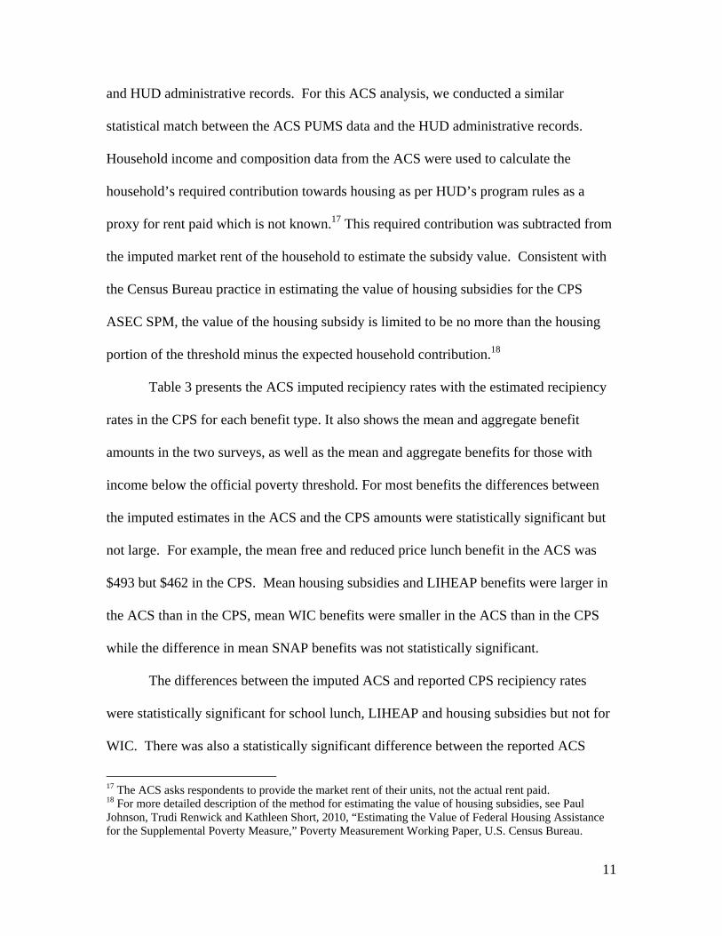
and HUD administrative records. For this ACS analysis, we conducted a similar
statistical match between the ACS PUMS data and the HUD administrative records.
Household income and composition data from the ACS were used to calculate the
household’s required contribution towards housing as per HUD’s program rules as a
proxy for rent paid which is not known.17 This required contribution was subtracted from
the imputed market rent of the household to estimate the subsidy value. Consistent with
the Census Bureau practice in estimating the value of housing subsidies for the CPS
ASEC SPM, the value of the housing subsidy is limited to be no more than the housing
portion of the threshold minus the expected household contribution.18
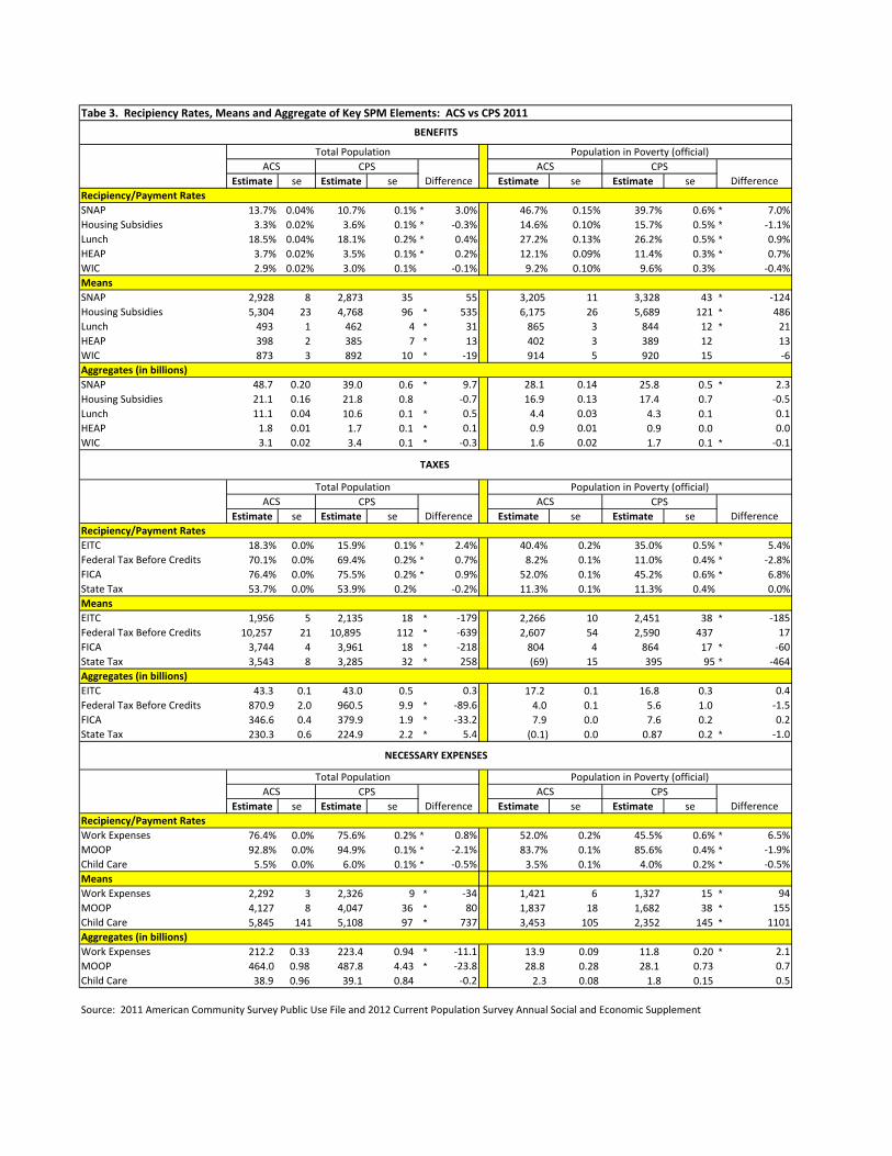
Table 3 presents the ACS imputed recipiency rates with the estimated recipiency
rates in the CPS for each benefit type. It also shows the mean and aggregate benefit
amounts in the two surveys, as well as the mean and aggregate benefits for those with
income below the official poverty threshold. For most benefits the differences between
the imputed estimates in the ACS and the CPS amounts were statistically significant but
not large. For example, the mean free and reduced price lunch benefit in the ACS was
$493 but $462 in the CPS. Mean housing subsidies and LIHEAP benefits were larger in
the ACS than in the CPS, mean WIC benefits were smaller in the ACS than in the CPS
while the difference in mean SNAP benefits was not statistically significant.
The differences between the imputed ACS and reported CPS recipiency rates
were statistically significant for school lunch, LIHEAP and housing subsidies but not for
WIC. There was also a statistically significant difference between the reported ACS
17 The ACS asks respondents to provide the market rent of their units, not the actual rent paid. 18 For more detailed description of the method for estimating the value of housing subsidies, see Paul Johnson, Trudi Renwick and Kathleen Short, 2010, “Estimating the Value of Federal Housing Assistance for the Supplemental Poverty Measure,” Poverty Measurement Working Paper, U.S. Census Bureau.

12
SNAP participation rate (13.7 percent) and the reported CPS SNAP participation rate
(10.7 percent). For units classified as poor using the official measure, the difference
between participation rates for WIC was not statistically significant but the participation
rate for housing subsidies was higher in the CPS than the ACS. Among the population in
poverty, the ACS imputed participation rates for school lunch and LIHEAP were higher
than the rates reported in the CPS.
Looking at the aggregate amounts, ACS estimates for SNAP, school lunch, and
LIHEAP were higher than the CPS estimates while the difference in the housing
subsidies was not statistically significant. The aggregate amount of WIC benefits in the
ACS was lower than in the CPS. For those categorized as poor using the official
measure, the differences in aggregate benefit amounts for housing subsidies, school lunch
and LIHEAP were not statistically significant. The aggregate amount for SNAP was
higher in the ACS than the CPS while the aggregate amount for WIC was higher in the
CPS than the ACS.
3. Tax Obligations and Tax Credits.
The SPM resource measure adds estimated values for tax credits and subtracts
estimated values for tax obligations. This paper estimates tax obligations and tax credits
using a tax calculator. For the CPS ASEC, the Census Bureau uses a tax calculator that
takes data from the CPS ASEC questionnaire enhanced with data from a statistical match
to Internal Revenue Service (IRS) data. This paper uses estimates from a similar tax
model developed for the Census Bureau designed to use ACS data. This process involves
forming tax units from ACS households (recognizing that ACS relationship data is more
limited than CPS ASEC relationship data but using the IPUMS-style relationship pointers

13
developed for this exercise) and dividing up some broader ACS income categories into
taxable and nontaxable income.
Table 3 provides some summary measures of the means and aggregate dollar
amounts for federal insurance contributions act (FICA) payroll tax, federal income tax
before credits, and the federal earned income tax credit. State taxes are also included in
the calculations. The table shows that a slightly higher percentage of units are assigned
payroll taxes overall in the ACS than in the CPS. For those classified as in poverty using
the official measure, 52 percent were assigned payroll taxes in the ACS while 45 percent
were assigned payroll taxes in the CPS. Average amounts assigned for payroll taxes are
slightly lower in the ACS for both groups.
Federal income taxes before credits show a different pattern. A greater percentage
of those below poverty using the official measure are assigned tax liability in the CPS.
Mean amounts are lower on average in the ACS compared to the CPS for the entire
population but the differences are not statistically significant for those below poverty
using the official measure. The aggregates amount for the total population is lower for the
ACS. For the population in poverty the difference in the aggregate amount of federal
taxes before credits was not statistically significant.
The EITC calculation results in a higher percentage of the total population and of
the official poor eligible for the EITC in the ACS than in the CPS. Average assigned
amounts are lower in the ACS than in the CPS, resulting in differences in the aggregate
amounts that were not statistically significant.
These estimates of tax liabilities are preliminary and there are clear improvements
that have been made in other work. More complex approaches have been used to form tax

14
units, improve estimates of tax deductions based on reporting housing expenses in the
ACS and divide “other income” into taxable and nontaxable portions.
4. Subtractions from Resources
The SPM uses thresholds derived from Consumer Expenditure Survey data on
spending on food, clothing, shelter and utilities. The ITWG suggested that Census
subtract expenditures on childcare, child support paid and medical out of pocket
expenditures from resources because these three key items are not included in the
thresholds and outlays for these purposes reduce the resources available to purchase the
expenditures categories included in the threshold. In order to estimate SPM poverty rates
in the ACS, the amounts to be subtracted from resources for these expenditures need to
be imputed. Child support paid is not included in this paper.19
4a. Child Care
This paper uses PROC MI with both the logistic and the predicted means
matching method to impute childcare expenditures. For childcare, the sample was
limited to those households with children age 13 and younger. For married-couple
households or households reporting an unmarried partner, the universe was limited to
households in which both the reference person and the spouse or partner were earners.
For unmarried household reference persons, the sample was limited to those in which the
reference person reported earnings. The logistic method was used to determine which
resource units paid for childcare. The predicted means matching method was used to
impute an amount to each resource unit.
19 In the CPS ASEC, the impact of child support paid is very small. The overall poverty rate for 2010 changed from 16.0 percent to 15.9 percent when child support paid was subtracted from resources.

15
For households designated as “paying for childcare,” the predicted weekly outlay
was multiplied by the number of weeks worked in the previous year by the reference
person, spouse or cohabiting partner with the least number of weeks worked.20 Since the
ACS public use data provides only categorical responses to the question on the number of
weeks worked, households were assigned the midpoint of the category as the number of
weeks worked. This same estimate of the number of weeks worked was used to assign
other work-related expenses using 85 percent of the median other work expenses reported
in the SIPP. Finally, work-related expenses including childcare were limited to be no
more than the earnings of the household reference person, spouse or cohabiting partner
with the lowest earnings. This limit is the same as the limit on work expenses used for the
CPS ASEC SPM estimates.
Table 3 compares summary statistics for the ACS imputed childcare outlays to the
reported childcare outlays from the CPS ASEC. While 6.0 percent of resource units
report some childcare expenses in the CPS ASEC, only 5.5 percent of resource units in
the ACS were designated as childcare payers. For all resource units and those in poverty,
the mean outlays for the ACS were higher than the mean outlays for the CPS. For
resource units with cash income below the official poverty thresholds, the mean imputed
amount was $3,453 as compared to the $2,352 reported in the CPS ASEC. The
differences in aggregate childcare amounts across the two samples were not statistically
significant for either the total population or those below the official poverty threshold.
The childcare imputation is less robust in the ACS due to the limited relationship
information. In the CPS ASEC there are parent pointers that enable one to cap childcare
20 The sample used to estimate the childcare amount was trimmed to eliminate the top 1 percentile of responses. This eliminated cases where the annual expenditures on childcare were reported to exceed $31,200.
16
and other work-related expenses at the earnings of the parent with the least amount of
earnings. In the ACS file the reference person, spouse or cohabiting partner of the
household may not be the parent of the child for whom childcare expenses are imputed.
The parent might work full time and pay for childcare for 52 weeks while the reference
person, spouse or cohabiting partner does not work at all. The method used in this
analysis would erroneously fail to impute childcare expenses to this household.
4b. Work Expenses
Table 3 also compares total work expenses. For this variable, 52 percent of
official poor resource units were assigned some expenses in the ACS as compared to
about 46 percent in the CPS ASEC. Mean amounts for the all resource units were lower
in the ACS but mean amounts for units in poverty were higher. The aggregate amount of
work-related expenses subtracted from ACS resource units was $11.1 billion less than the
CPS ASEC amount. For the officially poor population, the aggregate value of work
expenses were higher in the ACS than the CPS. One limitation of the ACS imputed work
expenses is the categorical nature of the weeks worked variable in the ACS public use
data.
4c. MOOP Models
For the SPM, medical out of pocket expenditures (MOOP) are subtracted from
resources before comparing resources to the poverty threshold. Since the CPS ASEC
includes specific questions on MOOP spending, these responses are used to estimate total
MOOP spending for each resource unit.

17
In this paper, the CPS ASEC data on MOOP are used to model expenditures on
health insurance premiums and other medical out of pocket outlays using PROC MI with
the predicted means match method. All imputations were done at the SPM unit level.
Outlays on premiums were set to $0 for individuals and families reporting no health
insurance or only Medicaid. PROC MI was used to estimate the amount of health
insurance premiums and other medical out of pocket expenditures.
Table 3 provides some summary statistics for the MOOP imputations and
compares these to reported MOOP expenditures from the CPS ASEC. In the CPS ASEC,
94.9 percent of resource units had some MOOP outlays. For the ACS the modeled
estimate is 92.8 percent, statistically different from the CPS ASEC estimate. For
officially poor resource units, the estimates are 85.6 percent and 83.7 percent. For both
the total sample and the officially poor resource units, the mean of the imputed ACS
MOOP is larger than the reported MOOP from the CPS ASEC. The total ACS imputed
MOOP is 23.8 billion dollars less than the CPS ASEC reported amount. For the
officially poor population, the difference in the aggregate MOOP imputed is not
statistically significant.
The MOOP imputations are constrained by the limited data available from the
ACS. The ACS does not ask about health status or receipt of disability payments, two
variables important in the MOOP model used in the NAS measures. In addition, the
health insurance questions are not directly comparable between the two surveys. The
CPS ASEC asks about health insurance at any time during the reference year. The ACS
asks about health insurance coverage at the time of the survey.
5. Thresholds.

18
The ACS is a continuous survey and asks respondents to report their income in
the previous 12 months. When calculating ACS estimates of poverty rates using the
official definition, the poverty thresholds vary by family size, age of reference person,
number of children and the month of the survey. Since this research uses the PUMS file
(which does not disclose the month of the survey), an annual threshold is used. In order to
be consistent with this threshold choice, the analysis uses the adjusted cash income
variable from the PUMS file.21
The ITWG suggested that the housing portion of the SPM thresholds be adjusted
for geographic differences in housing costs. 22 These adjustments factors are calculated
for specific metropolitan statistical areas with populations greater than 100,000. There is
a single average adjustment factor for smaller metropolitan areas in each state and one
adjustment factor for households outside metropolitan statistical areas in each state. Since
the ACS PUMS files does not identify metropolitan statistical areas, the adjustment
factors used for the 2011 research SPM estimates from the CPS ASEC were used with
the ACS 2011 internal file to calculate average geographic adjustment factors for each
PUMA. These adjustment factors were then assigned to each household based on the
location of the unit.
While PUMAs were selected as the geographic unit for the indices because this is
the smallest level of geography identifiable on the ACS PUMS file, the index values are
based on differences in housing costs across larger metropolitan areas. The April 2011
Urban Institute workshop included a discussion of the appropriate level of geography to
21 Thresholds are estimated by the Bureau of Labor Statistics and can be found at http://www.bls.gov/pir/spmhome.htm. 22 See Renwick, Trudi. Geographic Adjustments of Supplemental Poverty Measure Thresholds: Using the American Community Survey Five-Year Data on Housing Costs, July 2011, U.S. Census Bureau.

19
calculate the geographic indices. In that discussion there was concern that the geographic
unit should be larger than a single PUMA. The Urban Institute used Super-PUMAS in
their analysis. IRP aggregated PUMAs into larger regional units. NYC CEO used a
single geographic adjustment factor for all parts of New York City, in essence combining
numerous PUMAs.23
6. Preliminary SPM estimates
Table 4 compares official poverty rates to SPM rates by demographic group
including age, family type, race, Hispanic origin, nativity, tenure, region of residence and
health insurance status and compares the official poverty rates to the SPM rates for each
group. Table 5 compares the distribution of the poverty population across different
characteristics for each measure. Table 6 compares official poverty and SPM rates for
each state and the District of Columbia. Table 7 summarizes the effect of excluding
individual resource elements on SPM poverty rates in the ACS and CPS ASEC. Tables 8
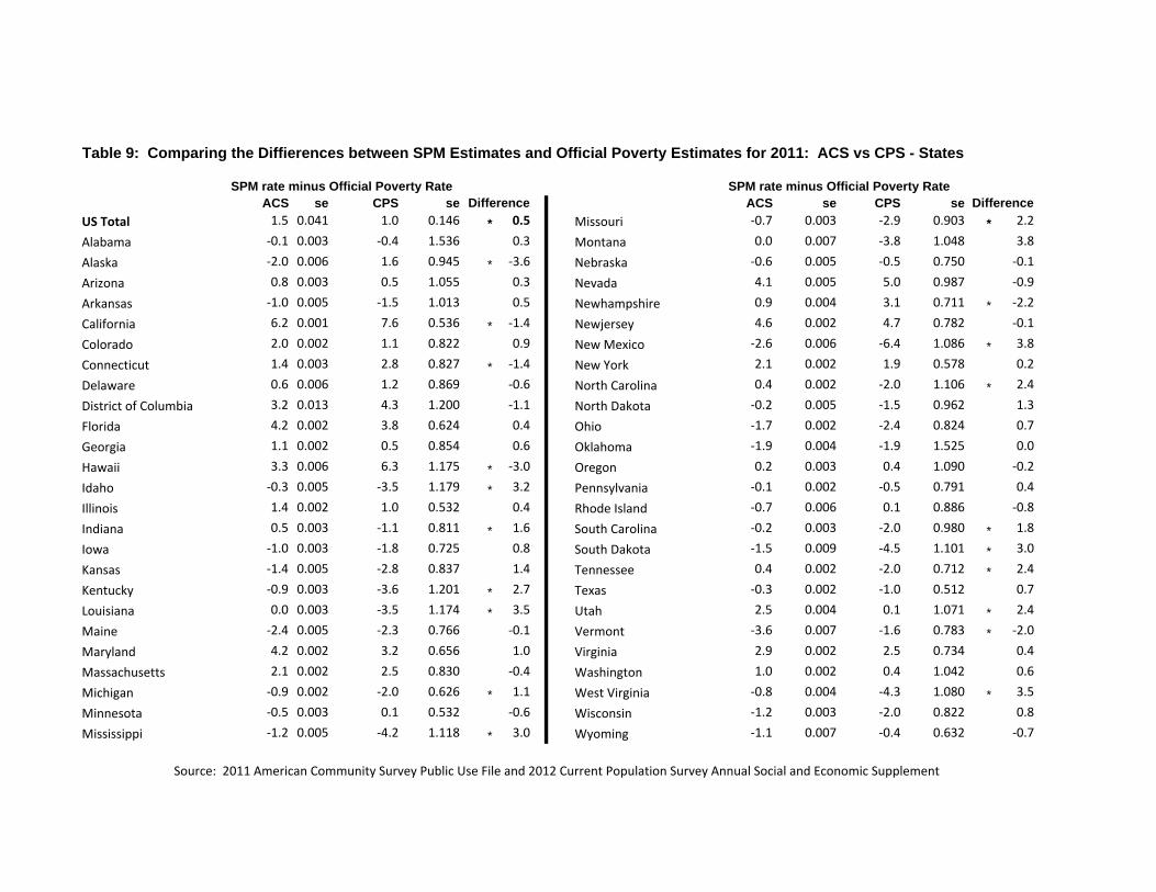
and 9 examine the “differences in differences” --- for specific demographic groups and
for each state, whether the difference between the SPM rate and the official poverty rates
in the ACS is different than the difference in the CPS ASEC.
For 2011, the SPM rate for the total population from the ACS was 17.4 percent
while the official poverty rate was 15.9 percent. There was a statistically significant
difference in the rates for every category included in Table 4 except the poverty rate for
those with a disability. The SPM rate was higher than the official rate for most groups.
The official poverty rate was higher than the SPM poverty rate for children, people in
new SPM resource units, Blacks, renters, people living in the Midwest, and people with
only public insurance. 23 Betson, Giannarelli and Zedlewski (2011) p. 6.

20
Since the overall SPM rate was higher than the official rate, it is not surprising
that the SPM rates were higher for most groups. Table 5 shows how the distribution of
the population in poverty differs across the two measures. For example, children were
35.4 percent of the official poor but 27.7 percent of the SPM poor. Other groups whose
share of the poor population shrank using the SPM include: people in female
householder units, people in new SPM units, Blacks, Hispanics, native born, renters,
people living in the Midwest, people living in the South, and people with only public
health insurance coverage. For all other groups in Table 5 the shares went up.
The SPM rate was statistically different from the official poverty rate in all but 12
states (Alabama, Delaware, Idaho, Louisiana, Nebraska, North Dakota, Oregon,
Pennsylvania, Rhode Island, South Carolina, Tennessee and Wyoming). The SPM rate
was higher than the official rate in: Arizona, California, Colorado, Connecticut, District
of Columbia, Florida, Georgia, Hawaii, Illinois, Indiana, Maryland, Massachusetts,
Nevada, New Hampshire, New Jersey, New York, North Carolina, Utah, Virginia and
Washington. For the other 19 states, the official poverty rate was higher than the SPM
rate.
For 2011, the SPM rate for the total population using the ACS was 17.4 percent,
higher than the 16.1 SPM rate from the CPS ASEC. The official rates also differed
across these surveys in 2011: 15.9 for the ACS vs. 15.1 in the CPS ASEC. There are
many reasons why the poverty estimates from the ACS would be distinguishable from the
CPS ASEC poverty estimates. These include differences in the reference period (the past
calendar year vs. the past 12 months), more detailed income-reporting categories in the

21
CPS ASEC than in the ACS, and mode of data collection.24 Despite these reservations, it
is important to assess to what extent these differences are a result of imprecise imputation
of the missing elements.
Table 7 examines the effect of each resource element on the overall SPM poverty
rate and the SPM poverty rates for specific age groups. For example, in the ACS the
SPM poverty rate without the EITC would be 19.4 percent rather than 17.4 percent. In
other words, adding the EITC to resources decreases the overall poverty rate by 2.1
percentage points. In the CPS, the impact of the EITC is to reduce the SPM poverty rate
from 18.0 percent to 16.1 percent, a decrease of about 2.0 percentage points. The
difference between the ACS marginal impact and the CPS ASEC marginal impact is not
statistically significant.
The marginal impact of SNAP benefits is higher in the ACS than in the CPS for
the total population, children and adults aged 18 to 64. This is consistent with the
estimates shown in Table 3. The ACS SNAP imputations add 9.2 billion more to
resources than the resources added in the CPS. In the case of SNAP, much of this is
driven by the higher participation rates in the ACS compared to the CPS. These are both
reported rates and not the result of our imputations.
The differences in the marginal impacts due to school lunch and LIHEAP and
were not statistically significant for any group. The marginal differences for WIC were
lower for adults aged 18 to 64, perhaps because there are some childless females (most
likely pregnant) receiving WIC benefits in the CPS ASEC who were not modeled in the
24 For more information on the differences between the ACS and CPS ASEC poverty estimates see http://www.census.gov/hhes/www/poverty/about/datasources/factsheet.html

22
ACS. Some of this may be the result of the less precise parent pointers in the ACS
which prevent us from correctly associating small children with their parents.
For the tax estimates, the differences in the marginal impacts for FICA and EITC
were not statistically significant. The differences in the marginal estimates for federal
taxes before credits were statistically significant but small.
For work expenses and MOOP almost all the differences in the marginal were
statistically significant. For work expenses, the ACS marginals were slightly greater than
the CPS estimates for the total population25 and each of the three age groups. Table 8
compares the difference between the SPM rate and the official poverty rate in the ACS to
the difference in the CPS ASEC for specific demographic groups. For the total
population and most demographic groups, the difference in the difference is statistically
significant. The differences are not statistically significant for whites, Hispanics, foreign
born, renters, those living in the Northeast and the West, people with only public health
insurance coverage and less than full-year, full-time workers. When the differences
between the ACS and the CPS are statistically significant, if they are higher in the ACS
they are also higher in the CPS and vice versa with the exception of people living in the
South. For people living in the South, the ACS SPM estimate is 1.0 percentage point
higher than the official estimate while in the CPS the SPM estimate is 0.1 percentage
point lower. Some of the statistically significant differences may be the result of
conceptual differences between the questions in the ACS and the CPS ASEC, e.g., health
insurance status and work experience.
25 The earlier version of this paper (presented at APPAM in November 2014) had a very large difference in the marginal impact of MOOP for the those aged 65 and older (7.0 percentage points). This revision to the models reduced that gap to 0.5 percentage points but the difference was still statistically significant.

23
Table 9 summarizes the differences between the SPM rates and the official
poverty rates for each of the 50 states and the District of Columbia. For twenty states the
differences are statistically significant. For sixteen of these twenty states (all but Alaska,
Indiana, North Carolina and Tennesssee) if the SPM was higher than the official rate in
the ACS it was also higher in the CPS ASEC and vice versa.
Future Research
There are several areas which should be investigated in future research, including:
Imputation of the parent pointers. In particular, why does our routine assign
fewer unrelated children to parents than the IPUMs pointers.
Assessment of whether or not using more than one year of CPS ASEC data in the
PROC MI procedures enhances the imputations.
MOOP and child care in the thresholds. Rather than imputing MOOP and child
care, we could include these in the thresholds. This is an approach that has been
used in several states and is worth considering for a national model.
Unit of analysis. Given the lack of relationship pointer, should we be using the
household as the unit of analysis rather than the SPM resource unit for ACS
estimates?
Taxes. Can we use TAXSIM26 rather than our own tax model for the tax
estimates?
The next step in the development of this public use file will be to take advantage of
the power of the multiple imputation process to produce multiple files. This would allow
users to estimate the variance introduced by the imputation process. Further research is
26 Feenberg (1993).

24
required to develop efficient methods of producing multiple imputations as well as
guidance to end users on how to use the multiple implicates.
Conclusion
This exercise has shown that using PROC MI is a reasonable approach to creating a
public use ACS SPM research file. While statistically different than the CPS ASEC SPM
rate for 2011, the difference between the two national rates is comparable to the
difference between the 2011 ACS and the CPS ASEC official national poverty rates.
Using this ACS file, we were able to report single year estimates of SPM rates for all 50
states and the District of Columbia. The marginal impacts of individual SPM resource
elements across the two surveys were not statistically significant for many of the
elements. Even when the differences in the marginal impacts were statistically
significant (SNAP, WIC, Federal Income Taxes before Credits, Work Expenses), the
differences were small.

25
References Allison, Paul D. Allison “Imputation of Categorical Variables with PROC MI,” Paper 113-30 SUGI 30. http://www2.sas.com/proceedings/sugi30/113-30.pdf Betson, David, Linda Giannarelli and Sheila R. Zedlewski. 2011. “Workshop on Poverty Measurement Using the American Community Survey.” Washington DC: Urban Institute. http://www.urban.org/publications/412396.html Citro, Constance F., and Robert T. Michael (eds.). 1995. Measuring Poverty: A New Approach. Washington, DC: National Academy Press. Feenberg, Daniel and Elizabeth Coutts. “An introduction to the TAXSIM model.” Journal of Policy Analysis and Management 12.1 (1993): 189-194. Garner, Thesia and Charles Hokayem,. 2012. “Supplemental Poverty Measure Thresholds: Imputing Noncash Benefits to the Consumer Expenditure Survey Using the Current Population Survey. U.S. Census Bureau and the Bureau of Labor Statistics. Paper presented at the November 2011 Southern Economic Association meetings in Washington, DC.
Hegeness, Misty, Trent Alexander and Sharon Stern. 2012. Measuring Families in Poverty: Using the American Community Survey to Construct Subfamily Units of Analysis for Local geographical Area Poverty Estimates. Paper presented at the 2012 Population Association of America meetings, San Francisco.
Iceland, John and David C. Ribar . March 2001. Measuring the Impact of Child Care Expenses on Poverty http://www.census.gov/hhes/povmeas/publications/work/childexp.pdf
Interagency Technical Working Group on Developing a Supplemental Poverty Measures. 2010. “Observations from the Interagency Technical Working Group on Developing a Supplemental Poverty Measure. http://www.census.gov/hhes/www/poverty/SPM_TWGObservations.pdf
Isaacs, Julia B, Joanna Y. Marks, Timothy M. Smeeding and Katherine A. Thornton. 2011. “Wisconsin Poverty Report: Methodology and Results for 2009,” Institute for Research on Poverty University of Wisconsin-Madison.
Johnson, Paul D, Trudi Renwick and Kathleen Short. 2011. Estimating the Value of Federal Housing Assistance for the Supplemental Poverty Measure. SEHSD Working Paper #2010-13. U.S. Census Bureau. Washington, DC.

26
Levitan, Mark and Trudi Renwick. 2010. Using the American Community Survey to Implement a National Academy of Sciences-Style Poverty Measure: A Comparison of Imputation Strategies. NYC Center for Economic Opportunity and U.S. Census Bureau. Paper presented at the August 2010 Annual Meeting of the American Statistical Association Section on Social Statistics, Vancouver, Canada. http://www.census.gov/hhes/povmeas/publications/overview/RenwickLevitanJSM2010.pdf
Mitchell, Josh. 2013. National SNAP Benefit Imputation in the American Community Survey: Assessing the Validity of Alternative Approaches. The Urban Institute.
New York City Center for Economic Opportunity. 2011. “Policy Affects Poverty: The CEO Poverty Measure 2005-2009: A Working Paper by the NYC Center for Economic Opportunity.
New York City Center for Economic Opportunity. 2010. “The CEO Poverty Measure, 2005-2008.” New York: NYC Center for Economic Opportunity.
O’Donnell, Sharon and Rodney Beard. 2009. “Imputing Medical Out-of-Pocket (MOOP) Expenditures using SIPP and MEPS.” U.S. Bureau of the Census. Paper presented at the August 2009 Annual Meeting of the American Statistical Association Section on Social Statistics.
O’Hara, Brett and Pat Doyle. 2001. The Impact of Imputation Strategies for Medical Out-of-Pocket Expenditures on Alternative Poverty Measures. U.S. Census Bureau Working Paper. http://www.census.gov/hhes/povmeas/publications/wp-medical.html
Passel, Jeffry. “Editing Family Data in Census 2000 Public-Use Microdata Samples: Creating Minimal Household Units (MHU’s).” (August 23, 2002).
Provencher, Ashley. 2011. “Unit of Analysis for Poverty Measurement: A Comparison of the Supplemental Poverty Measure and the Official Poverty Measure.” Paper presented at August 2011 Annual Meeting of the American Statistical Association.
Renwick, Trudi, Kathleen Short, Ale Bishaw and Charles Hokayem. 2012. “Using the American Community Survey (ACS) to Implement a Supplemental Poverty Measure.” U.S. Census Bureau, SEHSD Working Paper #2012-10.
Renwick, Trudi. 2011. Geographic Adjustments of Supplemental Poverty Measure Thresholds: Using the American Community Survey Five-Year Data on Housing Costs, SEHSD Working Paper Number 2011-21.U.S. Census Bureau.
Short, Kathleen. 2012. The Supplemental Poverty Measure: Examining the Incidence and Depth of Poverty in the U.S. Taking Account of Taxes and Transfers in 2010. U.S. Census Bureau: SEHSD Working Paper #2012-05. http://www.census.gov/hhes/povmeas/methodology/supplemental/research/sea2011.pdf
27
Short, Kathleen. 2013. The Research Supplemental Poverty Measure: 2012, U.S. Census Bureau, Current Population Reports, P60-247. Washington, DC.
Short, Kathleen. 2012. The Research Supplemental Poverty Measure: 2011, U.S. Census Bureau, Current Population Reports, P60-244. Washington, DC.
Short, Kathleen. 2011. The Research Supplemental Poverty Measure: 2010, U.S. Census Bureau, Current Population Reports, P60-241. Washington, DC.
Short, Kathleen. 2010. Experimental Modern Poverty Measures 2007. U.S. Census Bureau. Paper presented in a session sponsored by the Society of Government Economists at the Allied Social Science Association Meetings, Atlanta, Georgia.
Short, Kathleen. 2009. “Poverty Measures that Take Account of Changing Living Arrangements and Childcare Expenses.” U.S. Bureau of the Census, Paper presented at the August 2009 Annual Meeting of the American Statistical Association Section on Social Statistics. http://www.census.gov/hhes/povmeas/publications/taxes/childcareandcohab.jul24.pdf
Short, Kathleen and Thesia Garner, Davud Johnson and Patricia Doyle. 1999. Experimental Poverty Measures 1990-1997. U.S. Census Bureau, Current Population Reports, P60-205. Washington, DC.
Short, Kathleen. 2001. Experimental Poverty Measures: 1999. U.S. Census Bureau, Current Population Reports, P60-216. Washington, DC.
Zedlewski, Sheila, Linda Giannarelli, Laura Wheaton, and Joyce Morton. 2010. “Measuring Poverty at the State Level.” The Urban Institute

Table 1: Poverty Universe and Unit of Analysis(In Thousands)
Estimate SE Estimate SE
Total Poverty Universe* 303,586 0.2 302,685 17.7 * ‐900
Number of UI under 15 900 17.7 NA
Foster Children 174 5.0 NA
Other UI under 15 726 16.0 NA
Number of foster children 234 7.7 60 15.8 * ‐174
Under 15 174 5.0 NA
15 to 21 years of age 60 3.4 60 3.4 0
Number of cohabitors 6,722 28.9 NA
Number of Families/Resource Units 124,253 61.9 131,570 70.6 * 7,316
Multi‐person Families/Resource Units 80,298 90.0 83,077 84.0 * 2,779
Primary Families (includes household reference person) 79,924 91.3 83,077 84.0 * 3,154
Secondary Families 375 10.2 ‐
Single Person Resource Units 43,955 98.5 48,492 84.8 * 4,537
*Excluding group quarters
Source: 2011 American Community Survey Public Use File
SPM OfficialDifference

Household/Family Type
Single parent with a child Single parent with a child Single parent with a child Single parent with a child Single parent with a child Single parent with a child Single parent with a child Married head of SPM unit
Male head of SPM unit Male head of SPM unit Male head of SPM unit Male head of SPM unit Male head of SPM unit Male head of SPM unit Male head of SPM unit Elderly head of SPM unit
Elderly head of SPM unit Elderly head of SPM unit Elderly head of SPM unit
Household/Family Size
Presence of childrenNumber of children under 2
years of agePresence of children
Number of children 5 to 10
years of age
Number of children 5 to
10 years of agePresence of children
Number of children under
2 years of age
Number of adults in SPM
Unit
Number of people in the unitNumber of children 3 to 4 years
of age
Number of people in the
unit
Number of children 11 to
13 years of age
Number of children 11 to
13 years of age
Number of people in the
unit
Number of children 3 to 4
years of age
Number of children in SPM
unit
Number of children 5 to 10
years of age
Number of children 14 to
18 years of age
Number of children 14 to
18 years of age
One person (nonelderly)
SPM unit
Number of children 11 to 13
years of age
Age Age of unit head Age of unit head Age of unit head Age of unit head Age of unit head Age of unit head Age of unit head Age of unit head
Age squared Age squared Age squared Age squared Age squared Age squared Age squared Age squared
Less than a high school
eduction
Less than a high school
eduction
Less than a high school
eduction
Less than a high school
eduction
Less than a high school
eduction
Less than a high school
eduction
Less than a high school
eduction
High school diploma but did
not finish college
High school diploma but did not
finish college
High school diploma but did
not finish college
High school diploma but
did not finish college
High school diploma but
did not finish college
High school diploma but
did not finish college
High school diploma but
did not finish college
Income Log of cash income Log of cash income Log of cash income Log of cash income Log of cash income Log of cash income Log of cash income Log of cash income
Number of people reporting
Medicaid receipt
Number of people reporting
Medicaid receipt
Number of people
reporting Medicaid receipt
Number of people
reporting Medicaid receipt
Number of people
reporting Medicaid
receipt
Number of people
reporting Medicaid
receipt
Number of people
reporting Medicaid receipt
Number of people
reporting Medicaid receipt
Log of public assistance
incomeLog of public assistance income
Log of public assistance
income
Log of public assistance
income
Log of public assistance
income Log of public assistance
Log of public assistance
income
Number of people
reporting Medicare receipt
Receipt of SNAP Receipt of SNAP Receipt of SNAP Receipt of SNAP Receipt of SNAP Receipt of SNAP Number uninsured
Value of SNAP benefits Value of SNAP benefitsReceipt of housing
assistance
Receipt of housing
assistance
Number with employer
provided insurance
MOOP (logit and
PMM)
Program Participation
Educational Attainment
Table 2: Model Covariates by Benefit Type/Expenditure
Housing Assistance
(logit)
Child Care (logit and
pmm)
LIHEAP (logit and
pmm)
Subsidized Lunch
(logit)
Free or Reduced
Lunch (logit)SNAP (pmm) WIC (logit)
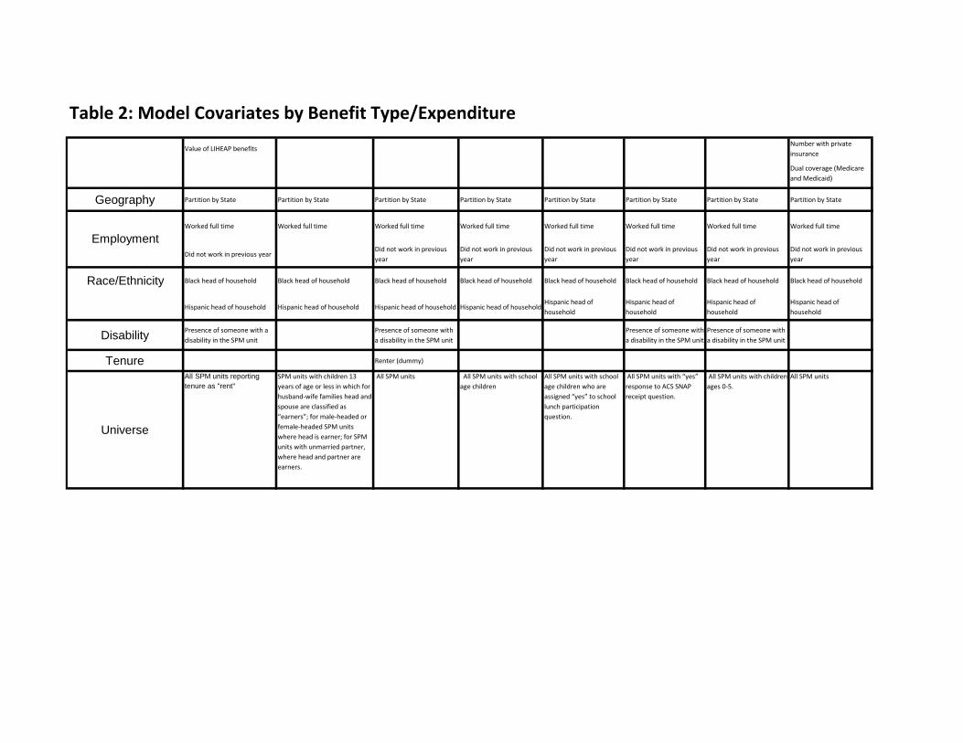
Table 2: Model Covariates by Benefit Type/Expenditure
Value of LIHEAP benefitsNumber with private
insurance
Dual coverage (Medicare
and Medicaid)
Geography Partition by State Partition by State Partition by State Partition by State Partition by State Partition by State Partition by State Partition by State
Worked full time Worked full time Worked full time Worked full time Worked full time Worked full time Worked full time Worked full time
Did not work in previous yearDid not work in previous
year
Did not work in previous
year
Did not work in previous
year
Did not work in previous
year
Did not work in previous
year
Did not work in previous
year
Race/Ethnicity Black head of household Black head of household Black head of household Black head of household Black head of household Black head of household Black head of household Black head of household
Hispanic head of household Hispanic head of household Hispanic head of household Hispanic head of householdHispanic head of
household
Hispanic head of
household
Hispanic head of
household
Hispanic head of
household
DisabilityPresence of someone with a
disability in the SPM unit
Presence of someone with
a disability in the SPM unit
Presence of someone with
a disability in the SPM unit
Presence of someone with
a disability in the SPM unit
Tenure Renter (dummy)
Universe
All SPM units reporting tenure as "rent"
SPM units with children 13
years of age or less in which for
husband‐wife families head and
spouse are classified as
“earners”; for male‐headed or
female‐headed SPM units
where head is earner; for SPM
units with unmarried partner,
where head and partner are
earners.
All SPM units All SPM units with school
age children
All SPM units with school
age children who are
assigned “yes” to school
lunch participation
question.
All SPM units with “yes”
response to ACS SNAP
receipt question.
All SPM units with children
ages 0‐5.
All SPM units
Employment
Tabe 3. Recipiency Rates, Means and Aggregate of Key SPM Elements: ACS vs CPS 2011
Estimate se Estimate se Estimate se Estimate se
SNAP 13.7% 0.04% 10.7% 0.1% * 3.0% 46.7% 0.15% 39.7% 0.6% * 7.0%
Housing Subsidies 3.3% 0.02% 3.6% 0.1% * ‐0.3% 14.6% 0.10% 15.7% 0.5% * ‐1.1%
Lunch 18.5% 0.04% 18.1% 0.2% * 0.4% 27.2% 0.13% 26.2% 0.5% * 0.9%
HEAP 3.7% 0.02% 3.5% 0.1% * 0.2% 12.1% 0.09% 11.4% 0.3% * 0.7%
WIC 2.9% 0.02% 3.0% 0.1% ‐0.1% 9.2% 0.10% 9.6% 0.3% ‐0.4%
SNAP 2,928 8 2,873 35 55 3,205 11 3,328 43 * ‐124
Housing Subsidies 5,304 23 4,768 96 * 535 6,175 26 5,689 121 * 486
Lunch 493 1 462 4 * 31 865 3 844 12 * 21
HEAP 398 2 385 7 * 13 402 3 389 12 13
WIC 873 3 892 10 * ‐19 914 5 920 15 ‐6
SNAP 48.7 0.20 39.0 0.6 * 9.7 28.1 0.14 25.8 0.5 * 2.3
Housing Subsidies 21.1 0.16 21.8 0.8 ‐0.7 16.9 0.13 17.4 0.7 ‐0.5
Lunch 11.1 0.04 10.6 0.1 * 0.5 4.4 0.03 4.3 0.1 0.1
HEAP 1.8 0.01 1.7 0.1 * 0.1 0.9 0.01 0.9 0.0 0.0
WIC 3.1 0.02 3.4 0.1 * ‐0.3 1.6 0.02 1.7 0.1 * ‐0.1
Estimate se Estimate se Estimate se Estimate se
EITC 18.3% 0.0% 15.9% 0.1% * 2.4% 40.4% 0.2% 35.0% 0.5% * 5.4%
Federal Tax Before Credits 70.1% 0.0% 69.4% 0.2% * 0.7% 8.2% 0.1% 11.0% 0.4% * ‐2.8%
FICA 76.4% 0.0% 75.5% 0.2% * 0.9% 52.0% 0.1% 45.2% 0.6% * 6.8%
State Tax 53.7% 0.0% 53.9% 0.2% ‐0.2% 11.3% 0.1% 11.3% 0.4% 0.0%
EITC 1,956 5 2,135 18 * ‐179 2,266 10 2,451 38 * ‐185
Federal Tax Before Credits 10,257 21 10,895 112 * ‐639 2,607 54 2,590 437 17
FICA 3,744 4 3,961 18 * ‐218 804 4 864 17 * ‐60
State Tax 3,543 8 3,285 32 * 258 (69) 15 395 95 * ‐464
EITC 43.3 0.1 43.0 0.5 0.3 17.2 0.1 16.8 0.3 0.4
Federal Tax Before Credits 870.9 2.0 960.5 9.9 * ‐89.6 4.0 0.1 5.6 1.0 ‐1.5
FICA 346.6 0.4 379.9 1.9 * ‐33.2 7.9 0.0 7.6 0.2 0.2
State Tax 230.3 0.6 224.9 2.2 * 5.4 (0.1) 0.0 0.87 0.2 * ‐1.0
Estimate se Estimate se Estimate se Estimate se
Work Expenses 76.4% 0.0% 75.6% 0.2% * 0.8% 52.0% 0.2% 45.5% 0.6% * 6.5%
MOOP 92.8% 0.0% 94.9% 0.1% * ‐2.1% 83.7% 0.1% 85.6% 0.4% * ‐1.9%
Child Care 5.5% 0.0% 6.0% 0.1% * ‐0.5% 3.5% 0.1% 4.0% 0.2% * ‐0.5%
Means
Work Expenses 2,292 3 2,326 9 * ‐34 1,421 6 1,327 15 * 94
MOOP 4,127 8 4,047 36 * 80 1,837 18 1,682 38 * 155
Child Care 5,845 141 5,108 97 * 737 3,453 105 2,352 145 * 1101
Work Expenses 212.2 0.33 223.4 0.94 * ‐11.1 13.9 0.09 11.8 0.20 * 2.1
MOOP 464.0 0.98 487.8 4.43 * ‐23.8 28.8 0.28 28.1 0.73 0.7
Child Care 38.9 0.96 39.1 0.84 ‐0.2 2.3 0.08 1.8 0.15 0.5
Source: 2011 American Community Survey Public Use File and 2012 Current Population Survey Annual Social and Economic Supplement
BENEFITS
TAXES
NECESSARY EXPENSES
Total Population Population in Poverty (official)
ACS CPS
Difference
ACS CPS
Difference
Recipiency/Payment Rates
Means
Aggregates (in billions)
Recipiency/Payment Rates
Means
Recipiency/Payment Rates
Aggregates (in billions)
Total Population Population in Poverty (official)
ACS CPS
Difference
ACS CPS
Difference
Aggregates (in billions)
Total Population Population in Poverty (official)
ACS CPS
Difference
ACS CPS
Difference

Table 4. Number and Percentage of People in Poverty by Different Poverty Measures: 2011
Number SE Percent SE Number SE Percent SE Number Percent
Total Population 303,586 52,762 181 17.38 0.06 48,354 184 15.93 0.06 4,407 * 1.5 *
Age ‐ ‐
Under 18 years 73,631 14,589 83 19.81 0.11 17,133 100 23.27 0.13 (2,544) * (3.5) *
18 to 64 years 190,041 31,587 103 16.62 0.05 27,577 94 14.51 0.05 4,010 * 2.1 *
65 years and older 39,914 6,586 32 16.50 0.08 3,644 21 9.13 0.05 2,941 * 7.4 *
Type of Unit ‐ ‐
Married couple 186,605 20,801 120 11.15 0.07 14,908 103 7.99 0.06 5,893 * 3.2 *
Female householder 63,046 19,570 102 31.04 0.14 18,608 98 29.52 0.13 962 * 1.5 *
Male householder 31,511 7,863 58 24.95 0.14 6,739 56 21.39 0.14 1,124 * 3.6 *
New SPM 22,424 4,527 51 20.19 0.21 8,099 65 36.12 0.22 (3,572) * (15.9) *
Race and Hispanic Origin ‐ ‐
White 225,632 32,596 122 14.45 0.05 29,278 136 12.98 0.06 3,318 * 1.5 *
White, not Hispanic 192,405 23,738 107 12.34 0.06 21,048 111 10.94 0.06 2,690 * 1.4 *
Black 37,435 10,286 66 27.48 0.18 10,420 64 27.83 0.17 (134) * (0.4) *
Asian 14,726 2,831 37 19.22 0.25 1,857 30 12.61 0.20 974 * 6.6 *
Hispanic (any race) 50,967 14,268 86 27.99 0.17 13,252 87 26.00 0.17 1,015 * 2.0 *
Nativity ‐ ‐
Native born 263,881 42,442 151 16.08 0.06 40,616 151 15.39 0.06 1,826 * 0.7 *
Foreign born 39,704 10,320 61 25.99 0.13 7,739 59 19.49 0.13 2,581 * 6.5 *
Naturalized citizen 17,950 3,287 27 18.31 0.15 2,027 21 11.29 0.11 1,260 * 7.0 *
Not a citizen 21,754 7,033 56 32.33 0.20 5,712 55 26.26 0.22 1,321 * 6.1 *
Tenure ‐ ‐
Owner 201,238 21,223 116 10.55 0.06 15,885 93 7.89 0.05 5,338 * 2.7 *
Owner/mortgage 146,642 13,460 101 9.18 0.07 9,398 77 6.41 0.05 4,063 * 2.8 *
Owner/no mortgage 59,687 9,314 55 15.60 0.08 8,172 54 13.69 0.09 1,142 * 1.9 *
Renter 97,256 29,987 158 30.83 0.11 30,784 173 31.65 0.11 (797) * (0.8) *
Region ‐ ‐
Northeast 53,816 8,053 56 14.96 0.10 7,142 52 13.27 0.10 911 * 1.7 *
Midwest 65,387 9,546 70 14.60 0.11 9,843 76 15.05 0.12 (296) * (0.5) *
South 113,095 21,015 102 18.58 0.09 19,837 90 17.54 0.08 1,178 * 1.0 *
West 71,287 14,147 88 19.85 0.12 11,533 80 16.18 0.11 2,614 * 3.7 *
Health Insurance Coverage ‐ ‐
With private coverage 192,816 16,460 74 8.54 0.04 10,485 62 5.44 0.04 5,975 * 3.1 *
With public, no private coverage 63,917 21,418 96 33.51 0.12 24,533 102 38.38 0.12 (3,114) * (4.9) *
Not insured 46,852 14,883 85 31.77 0.14 13,337 83 28.47 0.14 1,546 * 3.3 *
Disability Status ‐ ‐
Without a disability 170,912 26,421 98 15.46 0.06 22,398 89 13.11 0.05 4,023 * 2.4 *
With a disability 19,129 5,166 27 27.01 0.13 5,179 28 27.07 0.12 (13) * (0.1)
Work Experience ‐ ‐
All workers 146,293 16,822 66 11.50 0.05 13,250 55 9.06 0.04 3,572 * 2.4 *
Worked full‐time, year‐round 94,069 5,156 35 5.48 0.04 2,801 26 2.98 0.03 2,354 * 2.5 *
Les than full‐time year‐round 52,224 11,666 54 22.34 0.09 10,449 47 20.01 0.09 1,218 * 2.3 *
Did not work at least 1 week 43,747 14,765 62 33.75 0.11 14,327 61 32.75 0.11 438 * 1.0 *
Source: American Community Survey 2011
Supplemental Poverty Measure Official Poverty Measure DifferenceTotal (in
thousands)

Table 5. Distribution of People in Total and Poverty Populations: 2011
Characteristic Total SPM Official Difference/
Estimate SE Estimate SE Estimate SE
Age
Under 18 years 24.3 0.0 27.7 0.1 35.4 0.1 (7.8) *
18 to 64 years 62.6 0.0 59.9 0.1 57.0 0.1 2.8 *
65 years and older 13.2 0.0 12.5 0.1 7.5 0.0 4.9 *
Type of Unit
Married couple 61.5 0.1 39.4 0.2 30.8 0.2 8.6 *
Female householder 20.8 0.1 37.1 0.1 38.5 0.2 (1.4) *
Male householder 10.4 0.0 14.9 0.1 13.9 0.1 1.0 *
New SPM 7.4 0.0 8.6 0.1 16.8 0.1 (8.2) *
Race and Hispanic Origin
White 74.3 0.0 61.8 0.1 60.6 0.1 1.2 *
White, not Hispanic 63.4 0.0 45.0 0.1 43.5 0.1 1.5 *
Black 12.3 0.0 19.5 0.1 21.6 0.1 (2.1) *
Asian 4.9 0.0 5.4 0.1 3.8 0.1 1.5 *
Hispanic (any race) 16.8 0.0 27.0 0.1 27.4 0.1 (0.4) *
Nativity
Native born 86.9 0.0 80.4 0.1 84.0 0.1 (3.6) *
Foreign born 13.1 0.0 19.6 0.1 16.0 0.1 3.6 *
Naturalized citizen 5.9 0.0 6.2 0.1 4.2 0.0 2.0 *
Not a citizen 7.2 0.0 13.3 0.1 11.8 0.1 1.5 *
Tenure
Owner 66.3 0.1 40.2 0.2 32.9 0.2 7.4 *
Owner/mortgage 48.3 0.1 25.5 0.2 19.4 0.1 6.1 *
Owner/no mortgage 19.7 0.1 17.7 0.1 16.9 0.1 0.8 *
Renter 32.0 0.1 56.8 0.2 63.7 0.2 (6.8) *
Region
Northeast 17.7 0.0 15.3 0.1 14.8 0.1 0.5 *
Midwest 21.5 0.0 18.1 0.1 20.4 0.1 (2.3) *
South 37.3 0.0 39.8 0.1 41.0 0.1 (1.2) *
West 23.5 0.0 26.8 0.1 23.9 0.1 3.0 *
Health Insurance Coverage
With private coverage 63.5 0.1 31.2 0.1 21.7 0.1 9.5 *
With public, no private coverage 21.1 0.0 40.6 0.1 50.7 0.1 (10.1) *
Not insured 15.4 0.0 28.2 0.1 27.6 0.1 0.6 *
Source: American Community Survey 2011
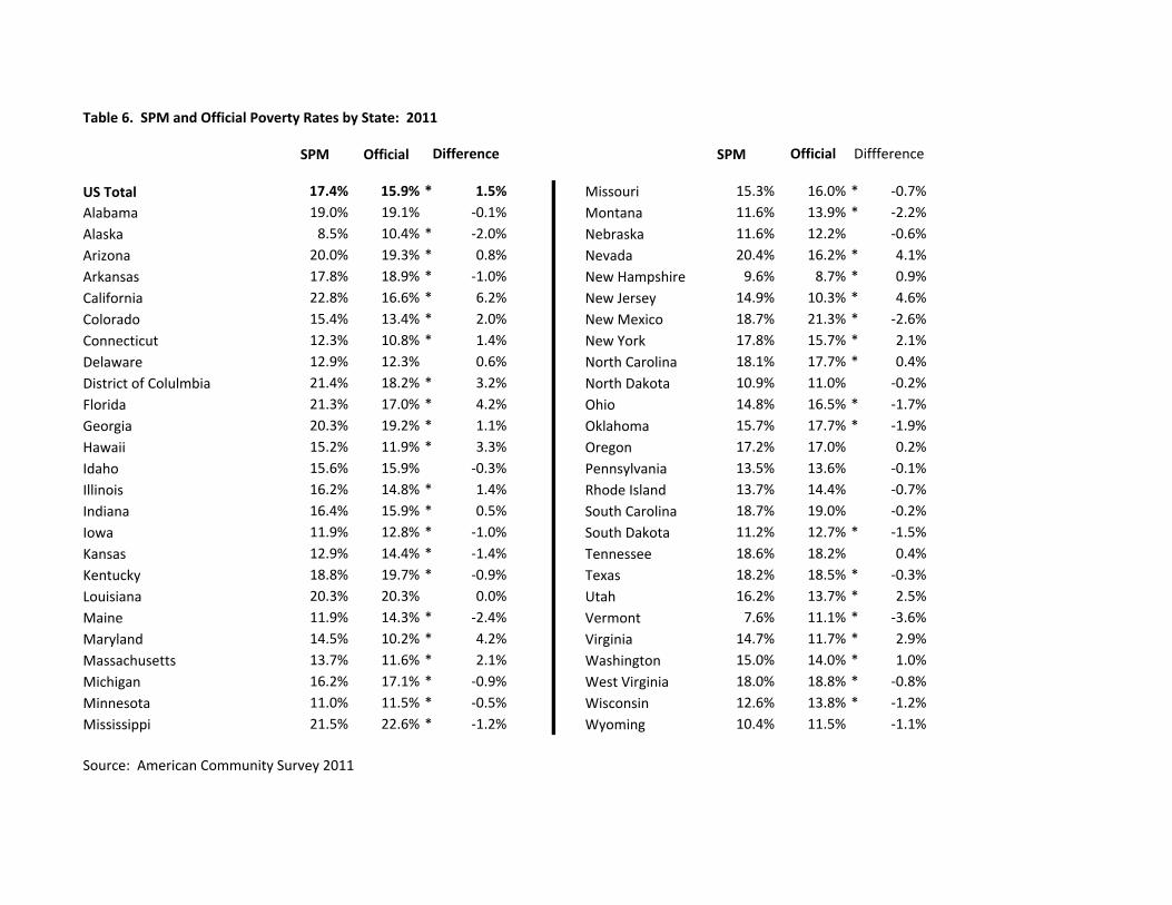
Table 6. SPM and Official Poverty Rates by State: 2011
SPM Official SPM
US Total 17.4% 15.9% * 1.5% Missouri 15.3% 16.0% * ‐0.7%
Alabama 19.0% 19.1% ‐0.1% Montana 11.6% 13.9% * ‐2.2%
Alaska 8.5% 10.4% * ‐2.0% Nebraska 11.6% 12.2% ‐0.6%
Arizona 20.0% 19.3% * 0.8% Nevada 20.4% 16.2% * 4.1%
Arkansas 17.8% 18.9% * ‐1.0% New Hampshire 9.6% 8.7% * 0.9%
California 22.8% 16.6% * 6.2% New Jersey 14.9% 10.3% * 4.6%
Colorado 15.4% 13.4% * 2.0% New Mexico 18.7% 21.3% * ‐2.6%
Connecticut 12.3% 10.8% * 1.4% New York 17.8% 15.7% * 2.1%
Delaware 12.9% 12.3% 0.6% North Carolina 18.1% 17.7% * 0.4%
District of Colulmbia 21.4% 18.2% * 3.2% North Dakota 10.9% 11.0% ‐0.2%
Florida 21.3% 17.0% * 4.2% Ohio 14.8% 16.5% * ‐1.7%
Georgia 20.3% 19.2% * 1.1% Oklahoma 15.7% 17.7% * ‐1.9%
Hawaii 15.2% 11.9% * 3.3% Oregon 17.2% 17.0% 0.2%
Idaho 15.6% 15.9% ‐0.3% Pennsylvania 13.5% 13.6% ‐0.1%
Illinois 16.2% 14.8% * 1.4% Rhode Island 13.7% 14.4% ‐0.7%
Indiana 16.4% 15.9% * 0.5% South Carolina 18.7% 19.0% ‐0.2%
Iowa 11.9% 12.8% * ‐1.0% South Dakota 11.2% 12.7% * ‐1.5%
Kansas 12.9% 14.4% * ‐1.4% Tennessee 18.6% 18.2% 0.4%
Kentucky 18.8% 19.7% * ‐0.9% Texas 18.2% 18.5% * ‐0.3%
Louisiana 20.3% 20.3% 0.0% Utah 16.2% 13.7% * 2.5%
Maine 11.9% 14.3% * ‐2.4% Vermont 7.6% 11.1% * ‐3.6%
Maryland 14.5% 10.2% * 4.2% Virginia 14.7% 11.7% * 2.9%
Massachusetts 13.7% 11.6% * 2.1% Washington 15.0% 14.0% * 1.0%
Michigan 16.2% 17.1% * ‐0.9% West Virginia 18.0% 18.8% * ‐0.8%
Minnesota 11.0% 11.5% * ‐0.5% Wisconsin 12.6% 13.8% * ‐1.2%
Mississippi 21.5% 22.6% * ‐1.2% Wyoming 10.4% 11.5% ‐1.1%
Official Diffference
Source: American Community Survey 2011
Difference

Table 7. Marginal Impacts of Key SPM Elements: Comparison of ACS to CPS for 2011
ACS SE CPS SE
SNAP Total Pop 1.79% 0.02% 1.54% 0.06% * 0.25%
Under 18 3.15% 0.05% 2.84% 0.14% * 0.31%
18 to 64 1.46% 0.02% 1.22% 0.05% * 0.24%
Over 65 0.86% 0.02% 0.74% 0.07% 0.12%
Housing Assistance Total Pop 0.67% 0.01% 0.95% 0.05% * ‐0.29%
Under 18 0.95% 0.03% 1.40% 0.10% * ‐0.45%
18 to 64 0.50% 0.01% 0.73% 0.04% * ‐0.22%
Over 65 0.91% 0.02% 1.20% 0.10% * ‐0.29%
School Lunch Total Pop 0.36% 0.01% 0.35% 0.03% 0.01%
Under 18 0.85% 0.03% 0.86% 0.08% ‐0.01%
18 to 64 0.24% 0.01% 0.22% 0.02% 0.02%
Over 65 0.03% 0.00% 0.03% 0.01% ‐0.01%
WIC Total Pop 0.12% 0.01% 0.15% 0.02% ‐0.03%
Under 18 0.29% 0.02% 0.34% 0.05% ‐0.04%
18 to 64 0.08% 0.00% 0.11% 0.02% * ‐0.03%
Over 65 0.01% 0.00% 0.00% 0.00% 0.00%
LIHEAP Total Pop 0.05% 0.00% 0.06% 9.76E‐05 0.00%
Under 18 0.07% 0.01% 0.05% 0.02% 0.02%
18 to 64 0.05% 0.00% 0.05% 0.01% 0.00%
Over 65 0.05% 0.00% 0.08% 0.02% ‐0.03%
ACS SE CPS SE
EITC Total Pop 2.06% 0.02% 1.98% 0.07% 0.07%
Under 18 4.36% 0.05% 4.20% 0.16% 0.16%
18 to 64 1.57% 0.02% 1.53% 0.06% 0.03%
Over 65 0.15% 0.01% 0.12% 0.03% 0.03%
FICA Total Pop ‐1.27% 0.02% ‐1.28% 0.06% 0.02%
Under 18 ‐1.62% 0.03% ‐1.70% 0.10% 0.08%
18 to 64 ‐1.34% 0.02% ‐1.35% 0.06% 0.01%
Over 65 ‐0.30% 0.01% ‐0.25% 0.04% ‐0.05%Federal Income Taxes
Before Credits Total Pop‐0.42% 0.01% ‐0.48% 0.03%
* 0.06%
Under 18 ‐0.41% 0.01% ‐0.30% 0.04% * ‐0.11%
18 to 64 ‐0.49% 0.01% ‐0.60% 0.04% * 0.11%
Over 65 ‐0.12% 0.01% ‐0.26% 0.06% * 0.13%
ACS SE CPS SE
MOOP Total Pop ‐3.74% 0.03% ‐3.39% 0.09% * ‐0.35%
Under 18 ‐3.13% 0.04% ‐2.80% 0.14% * ‐0.33%
18 to 64 ‐3.19% 0.03% ‐2.83% 0.09% * ‐0.36%
Over 65 ‐7.48% 0.05% ‐7.03% 0.24% * ‐0.44%
Work Expenses Total Pop ‐1.84% 0.02% ‐1.67% 0.06% * ‐0.17%
Under 18 ‐2.54% 0.04% ‐2.27% 0.12% * ‐0.27%
18 to 64 ‐1.87% 0.02% ‐1.73% 0.07% * ‐0.14%
Over 65 ‐0.43% 0.01% ‐0.32% 0.04% * ‐0.10%
Source: American Community Survey 2011
BENEFITS
Difference
Difference
TAXES
NECESSARY EXPENDITURES
Difference

ACS se CPS seTotal Population 1.5 0.04 1.0 0.15 * 0.5
Age
Under 18 years -3.5 0.09 -4.3 0.28 * 0.8
18 to 64 years 2.1 0.04 1.8 0.14 * 0.3
65 years and older 7.4 0.07 6.3 0.27 * 1.1
Type of Unit 0.0
Married couple 3.2 0.04 2.5 0.17 * 0.7
Female householder 1.5 0.11 0.3 0.35 * 1.2
Male householder 3.6 0.10 4.6 0.32 * -1.0
New SPM -15.9 0.21 -12.5 0.61 * -3.4
Race and Hispanic Origin 0.0
White 1.5 0.04 1.3 0.15 0.2
White, not Hispanic 1.4 0.04 1.0 0.14 * 0.4
Black -0.4 0.13 -2.1 0.45 * 1.7
Asian 6.6 0.18 4.6 0.59 * 2.0
Hispanic (any race) 2.0 0.13 2.4 0.49 -0.4
Nativity 0.0
Native born 0.7 0.04 0.1 0.15 * 0.6
Foreign born 6.5 0.10 6.7 0.38 -0.2
Naturalized citizen 7.0 0.12 5.8 0.45 * 1.2
Not a citizen 6.1 0.18 7.5 0.55 * -1.4
Tenure 0.0
Owner 2.7 0.04 1.8 0.14 * 0.9
Owner/mortgage 2.8 0.05 2.3 0.16 * 0.5
Owner/no mortgage 1.9 0.07 0.5 0.24 * 1.4
Renter -0.8 0.09 -0.6 0.35 -0.2
Region 0.0
Northeast 1.7 0.09 1.8 0.32 -0.1
Midwest -0.5 0.09 -1.3 0.24 * 0.8
South 1.0 0.07 -0.1 0.24 * 1.1
West 3.7 0.09 4.1 0.35 -0.4
Health Insurance Coverage 0.0
With private coverage 3.1 0.03 2.6 0.13 * 0.5
With public, no private coverage -4.9 0.11 -5.5 0.38 0.6
Not insured 3.3 0.12 2.6 0.40 * 0.7
Disability Status 0.0
Without a disability 2.4 0.04 1.1 0.15 * 1.3
With a disability -0.1 0.12 -1.2 0.49 * 1.1
Work Experience 0.0
All workers 2.4 0.04 2.2 0.12 * 0.2
Worked full‐time, year‐round 2.5 0.03 2.3 0.11 * 0.2
Les than full‐time year‐round 2.3 0.09 2.1 0.26 0.2
Did not work at least 1 week 1.0 0.08 0.2 0.30 * 0.8
Table 8: Comparing the Diffierences between SPM Estimates and Official Poverty Estimates for 2011: ACS vs CPS
SPM rate minus Official Poverty Rate Difference
Source: 2011 American Community Survey Public Use File and 2012 Current Population
Survey Annual Social and Economic Supplement
ACS se CPS se ACS se CPS se
US Total 1.5 0.041 1.0 0.146 * 0.5 Missouri ‐0.7 0.003 ‐2.9 0.903 * 2.2
Alabama ‐0.1 0.003 ‐0.4 1.536 0.3 Montana 0.0 0.007 ‐3.8 1.048 3.8
Alaska ‐2.0 0.006 1.6 0.945 * ‐3.6 Nebraska ‐0.6 0.005 ‐0.5 0.750 ‐0.1
Arizona 0.8 0.003 0.5 1.055 0.3 Nevada 4.1 0.005 5.0 0.987 ‐0.9
Arkansas ‐1.0 0.005 ‐1.5 1.013 0.5 Newhampshire 0.9 0.004 3.1 0.711 * ‐2.2
California 6.2 0.001 7.6 0.536 * ‐1.4 Newjersey 4.6 0.002 4.7 0.782 ‐0.1
Colorado 2.0 0.002 1.1 0.822 0.9 New Mexico ‐2.6 0.006 ‐6.4 1.086 * 3.8
Connecticut 1.4 0.003 2.8 0.827 * ‐1.4 New York 2.1 0.002 1.9 0.578 0.2
Delaware 0.6 0.006 1.2 0.869 ‐0.6 North Carolina 0.4 0.002 ‐2.0 1.106 * 2.4
District of Columbia 3.2 0.013 4.3 1.200 ‐1.1 North Dakota ‐0.2 0.005 ‐1.5 0.962 1.3
Florida 4.2 0.002 3.8 0.624 0.4 Ohio ‐1.7 0.002 ‐2.4 0.824 0.7
Georgia 1.1 0.002 0.5 0.854 0.6 Oklahoma ‐1.9 0.004 ‐1.9 1.525 0.0
Hawaii 3.3 0.006 6.3 1.175 * ‐3.0 Oregon 0.2 0.003 0.4 1.090 ‐0.2
Idaho ‐0.3 0.005 ‐3.5 1.179 * 3.2 Pennsylvania ‐0.1 0.002 ‐0.5 0.791 0.4
Illinois 1.4 0.002 1.0 0.532 0.4 Rhode Island ‐0.7 0.006 0.1 0.886 ‐0.8
Indiana 0.5 0.003 ‐1.1 0.811 * 1.6 South Carolina ‐0.2 0.003 ‐2.0 0.980 * 1.8
Iowa ‐1.0 0.003 ‐1.8 0.725 0.8 South Dakota ‐1.5 0.009 ‐4.5 1.101 * 3.0
Kansas ‐1.4 0.005 ‐2.8 0.837 1.4 Tennessee 0.4 0.002 ‐2.0 0.712 * 2.4
Kentucky ‐0.9 0.003 ‐3.6 1.201 * 2.7 Texas ‐0.3 0.002 ‐1.0 0.512 0.7
Louisiana 0.0 0.003 ‐3.5 1.174 * 3.5 Utah 2.5 0.004 0.1 1.071 * 2.4
Maine ‐2.4 0.005 ‐2.3 0.766 ‐0.1 Vermont ‐3.6 0.007 ‐1.6 0.783 * ‐2.0
Maryland 4.2 0.002 3.2 0.656 1.0 Virginia 2.9 0.002 2.5 0.734 0.4
Massachusetts 2.1 0.002 2.5 0.830 ‐0.4 Washington 1.0 0.002 0.4 1.042 0.6
Michigan ‐0.9 0.002 ‐2.0 0.626 * 1.1 West Virginia ‐0.8 0.004 ‐4.3 1.080 * 3.5
Minnesota ‐0.5 0.003 0.1 0.532 ‐0.6 Wisconsin ‐1.2 0.003 ‐2.0 0.822 0.8
Mississippi ‐1.2 0.005 ‐4.2 1.118 * 3.0 Wyoming ‐1.1 0.007 ‐0.4 0.632 ‐0.7
Difference
Table 9: Comparing the Diffierences between SPM Estimates and Official Poverty Estimates for 2011: ACS vs CPS - States
Source: 2011 American Community Survey Public Use File and 2012 Current Population Survey Annual Social and Economic Supplement
SPM rate minus Official Poverty RateDifference
SPM rate minus Official Poverty Rate