ut testing add01a equipment calibrations
Post on 20-Jul-2016
63 views
DESCRIPTION
My ASNT UT Level III Pre-exam Study notes. Not proven yet! The exam is due next month.TRANSCRIPT

Addendum-01aEquipment Calibrations My ASNT Level III UT Study Notes.2014-June


http://en.wikipedia.org/wiki/Greek_alphabet

Speaker: Fion Zhang2014/6/19

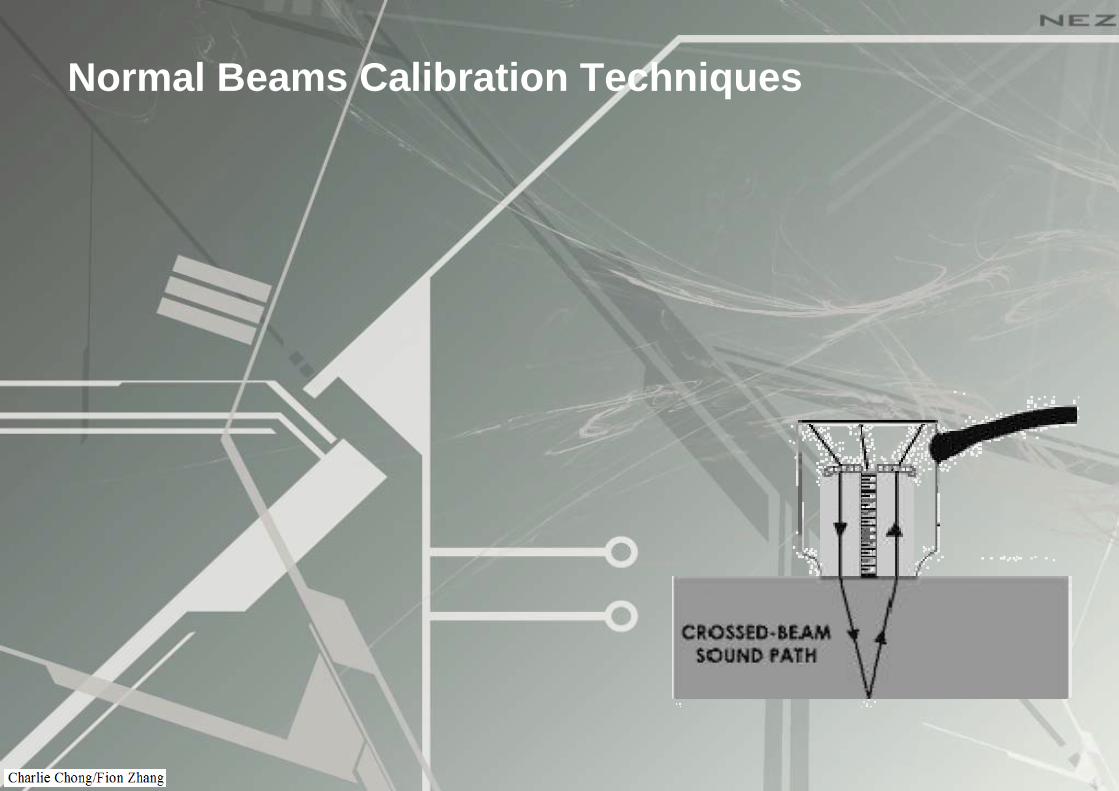
Normal Beams Calibration Techniques

Attenuation due to Beam spread for: Large Reflector Small Reflector
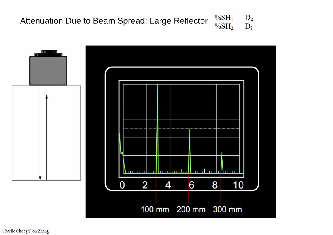
Attenuation Due to Beam Spread: Large Reflector

Attenuation Due to Beam Spread: Small Reflector
D2
D1
SH1
SH2
Material Attenuation Determination:

Material Attenuation Determination: Actual BWE display

IF zero Material attenuation: The second BWE at twice the distance will be exactly 6dB less (50% less), half the 1st BWE height ( ½ FSH). However this is never the case!

Δ dB = total Material attenuation at twice distance travel.
Material attenuation =
D2D1
ΔdB
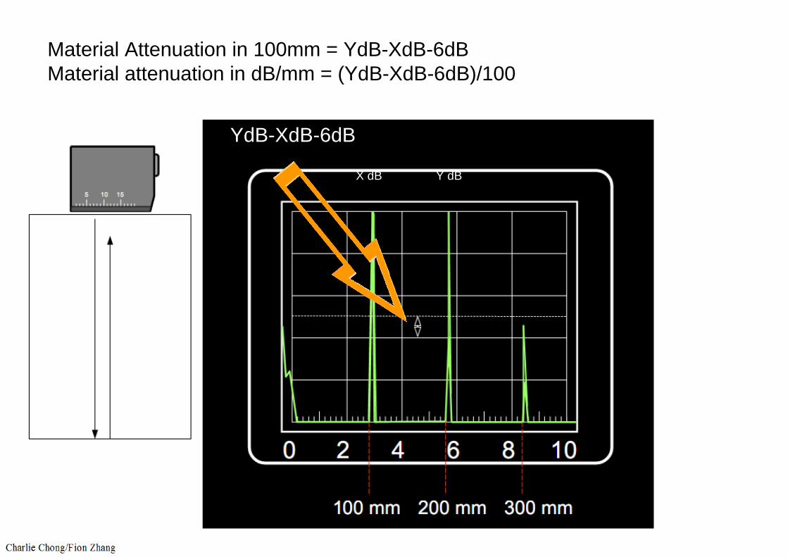
Material Attenuation in 100mm = YdB-XdB-6dBMaterial attenuation in dB/mm = (YdB-XdB-6dB)/100
Y dBX dB
YdB-XdB-6dB
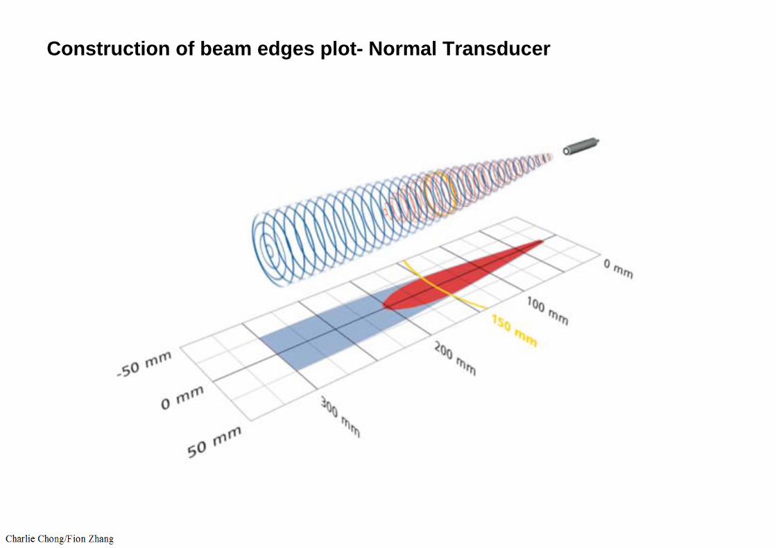
Construction of beam edges plot- Normal Transducer
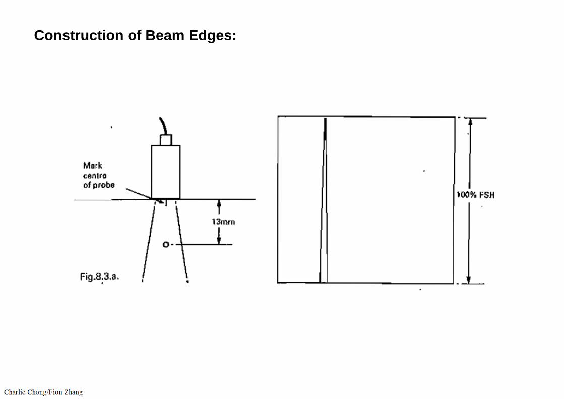
Construction of Beam Edges:
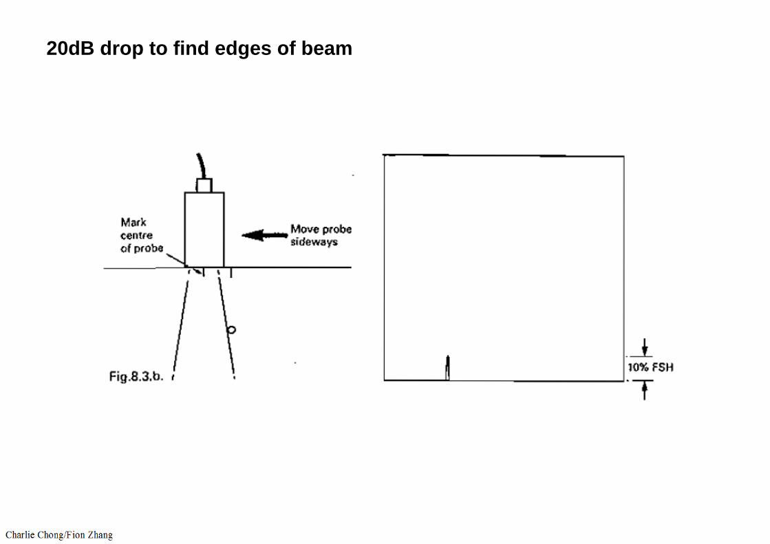
20dB drop to find edges of beam
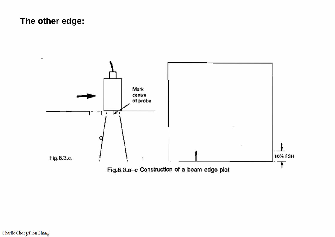
The other edge:

Construction of beam spread at 13mm:
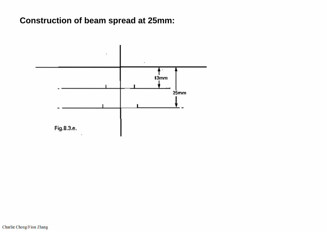
Construction of beam spread at 25mm:
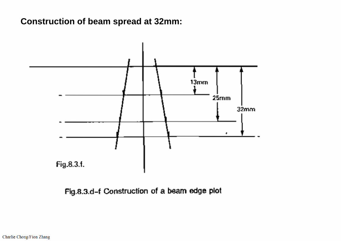
Construction of beam spread at 32mm:
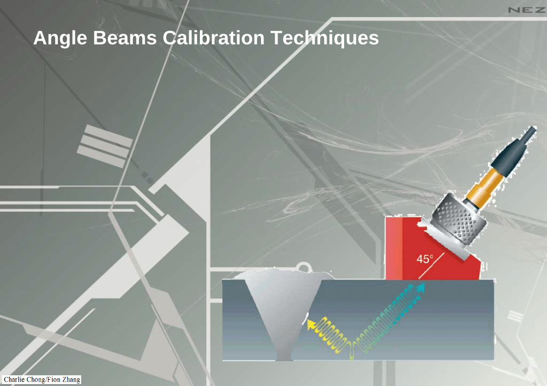
Angle Beams Calibration Techniques
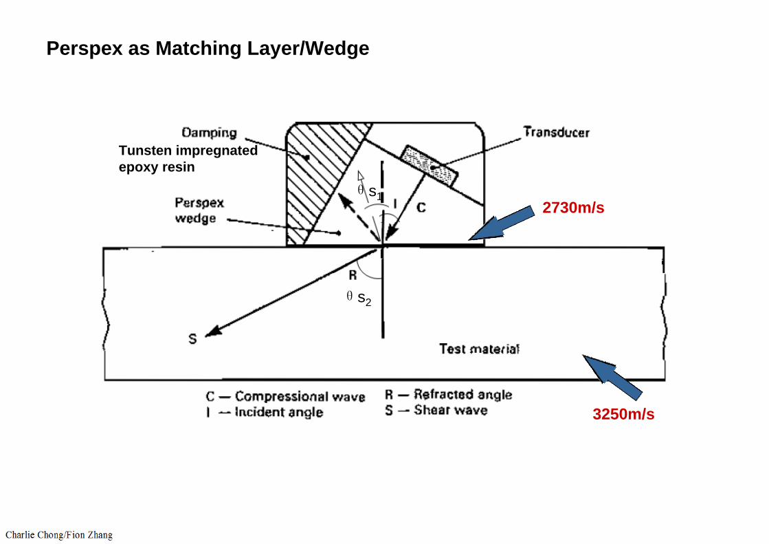
Perspex as Matching Layer/Wedge
2730m/s
3250m/s
θs1
θs2
Tunsten impregnated epoxy resin

Perspex as Matching Layer/Wedge
1. The Shear wave velocity of Perspex is 2730m/s, the shear wave velocity od steel is 3250m/s. The refracted angle of Perspex ϴS1 is always smaller than ϴS2
2. Pespex is very absortive and attenuated efficiently, thus reflected compressional wavw will be dampen.
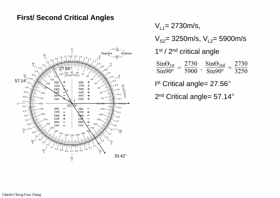
First/ Second Critical Angles
B
VL1= 2730m/s,
VS2= 3250m/s, VL2= 5900m/s
1st / 2nd critical angle
Ist Critical angle= 27.56°
2nd Critical angle= 57.14°°
27.56°
57.14°
33.42°
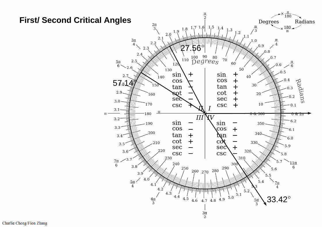
First/ Second Critical Angles
°
27.56°
57.14°
33.42°
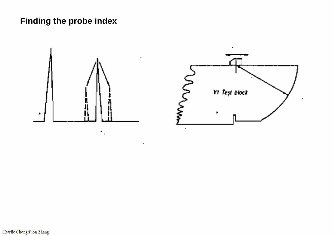
Finding the probe index

Finding the probe index

Checking the probe Angle:
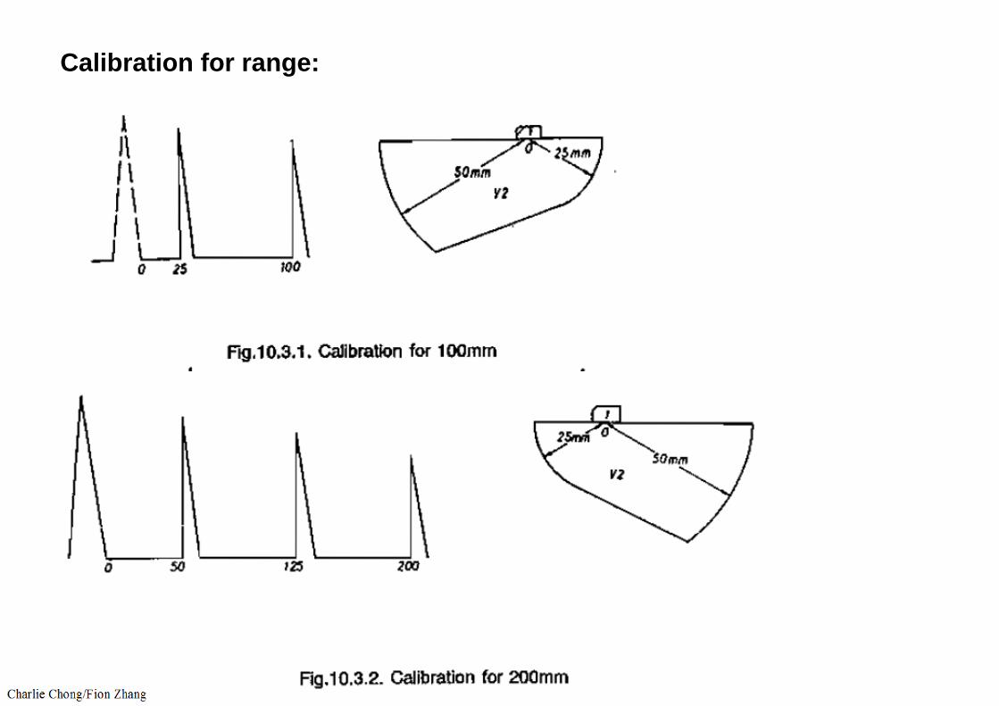
Calibration for range:
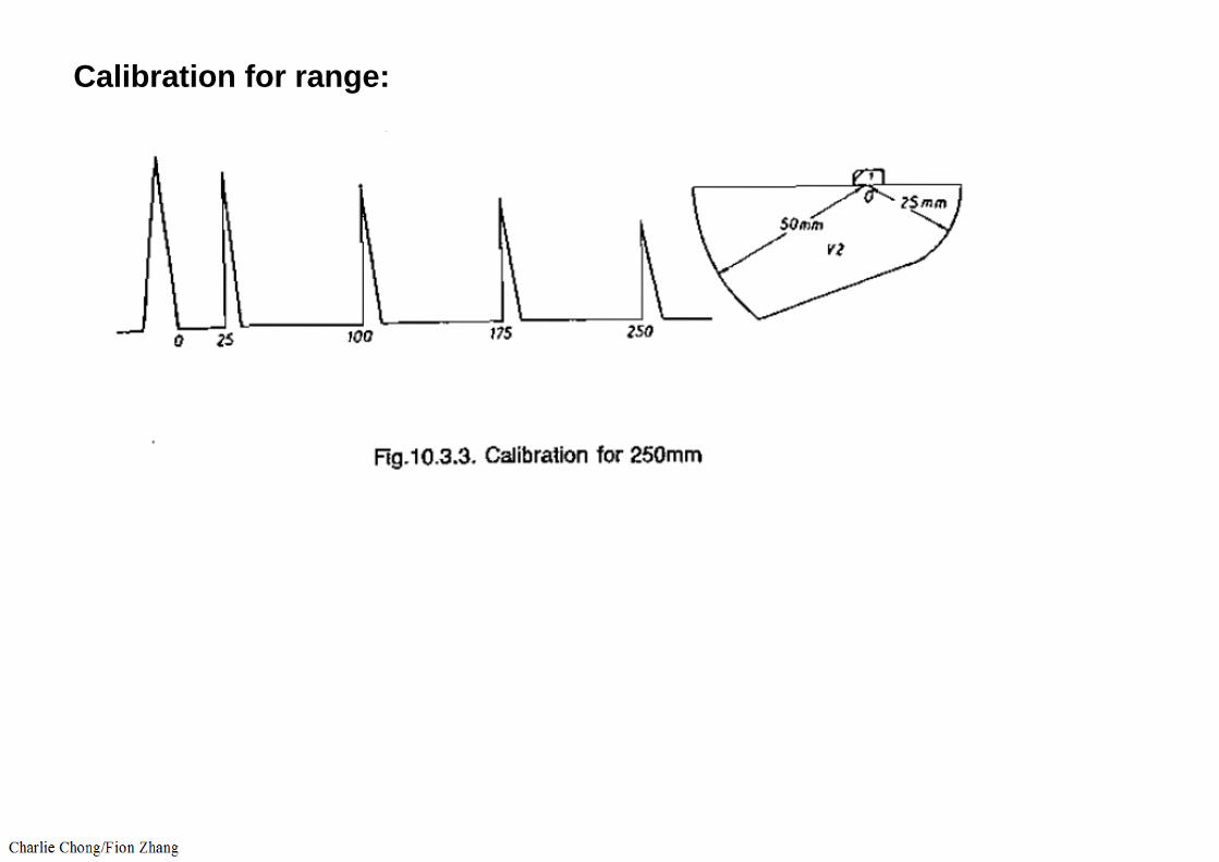
Calibration for range:
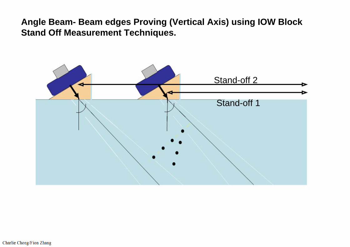
Angle Beam- Beam edges Proving (Vertical Axis) using IOW BlockStand Off Measurement Techniques.
Stand off 2
Stand-off 2
Stand-off 1
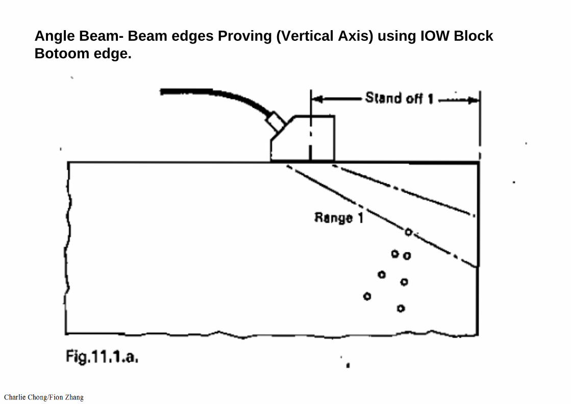
Angle Beam- Beam edges Proving (Vertical Axis) using IOW BlockBotoom edge.
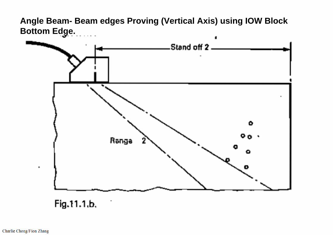
Angle Beam- Beam edges Proving (Vertical Axis) using IOW BlockBottom Edge.

The IOW Block: The Institute of Welding Block
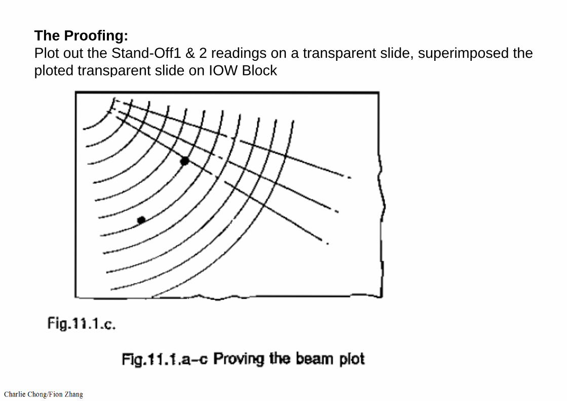
The Proofing:Plot out the Stand-Off1 & 2 readings on a transparent slide, superimposed the ploted transparent slide on IOW Block
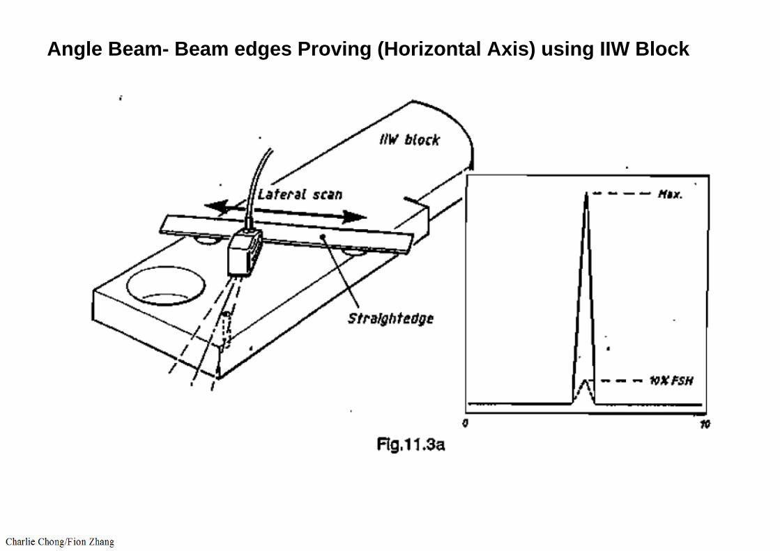
Angle Beam- Beam edges Proving (Horizontal Axis) using IIW Block

Angle Beam- Beam edges Proving (Horizontal Axis) using IIW Block

Angle Beam- Beam edges Proving (Horizontal Axis) using IIW Block
Scanned at ½ , 1, 1 ½ Skips

Angle Beam- Beam edges Proving (Horizontal Axis) using IIW Block

Angle Beam- Beam edges Proving (Horizontal Axis) using IIW Block
½ Skip
1 Skip1½ Skip
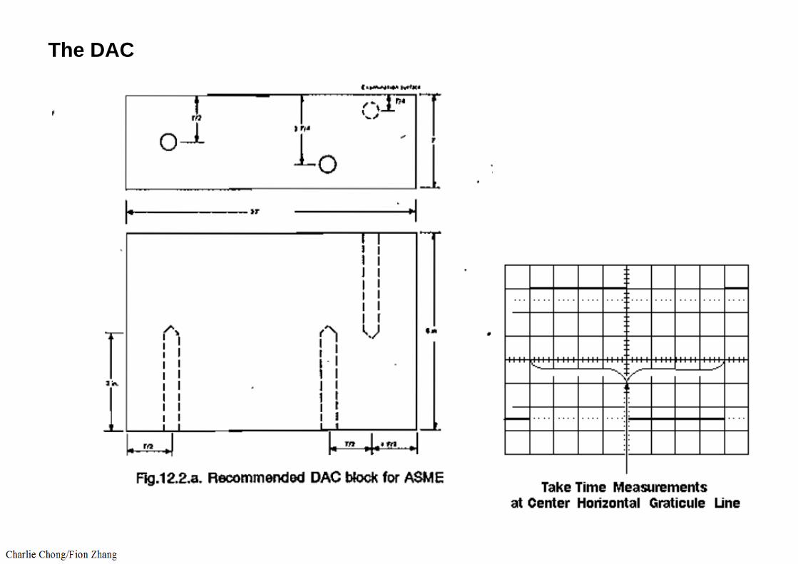
The DAC
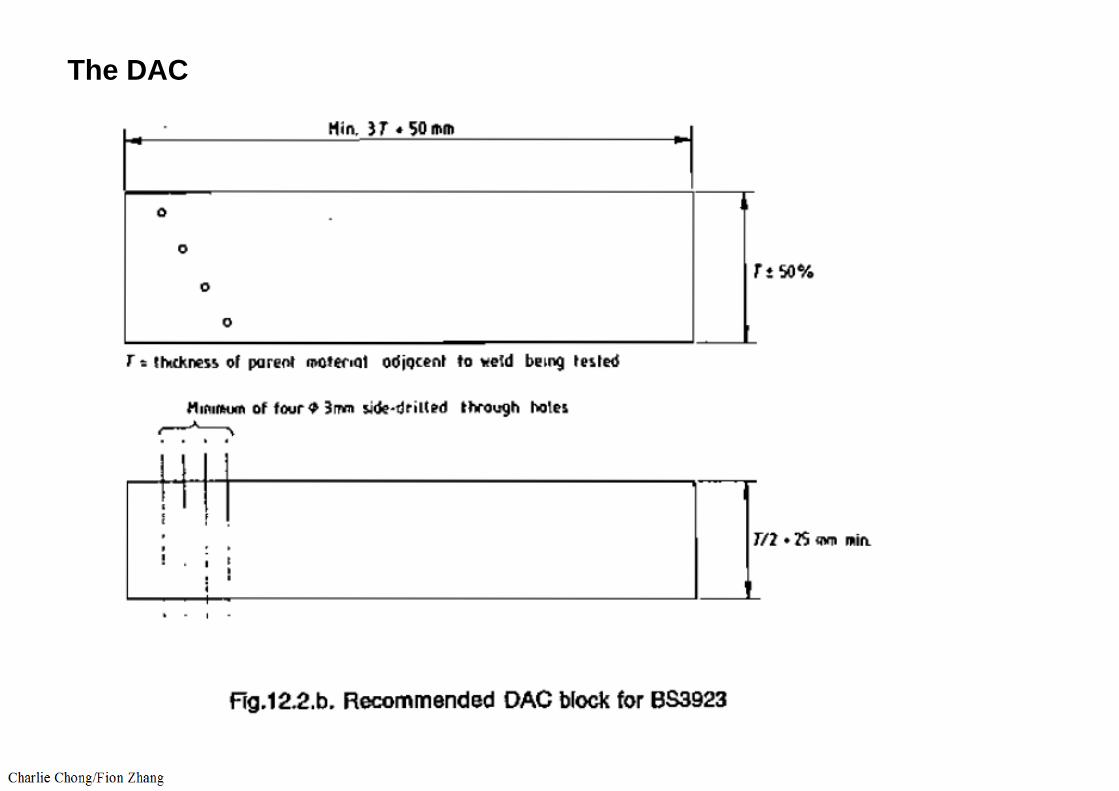
The DAC

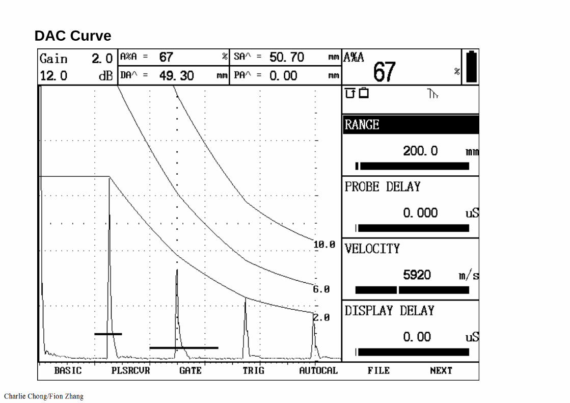
DAC Curve
DAC Curve

DAC Curve Plot
1. Obtained the signal from the refernce reflector and mark on the graticule/traspatrent sheet with gain setting at 80% FSH.
2. Set the gain control -6bB and marks the 50% mark.
3. Set the gain contril to the
4. Obtained the signal at the gain setting in item 1 and repeat the process at different sound paths.
5. Plot the curves at the gain setting and -6dB.
6. Determined the transfer correction.
7. Scanned the work pieces at the “Gain Setting + Transfer Correction”

FLAT Bottom Holes FBH

FLAT Bottom Holes FBH
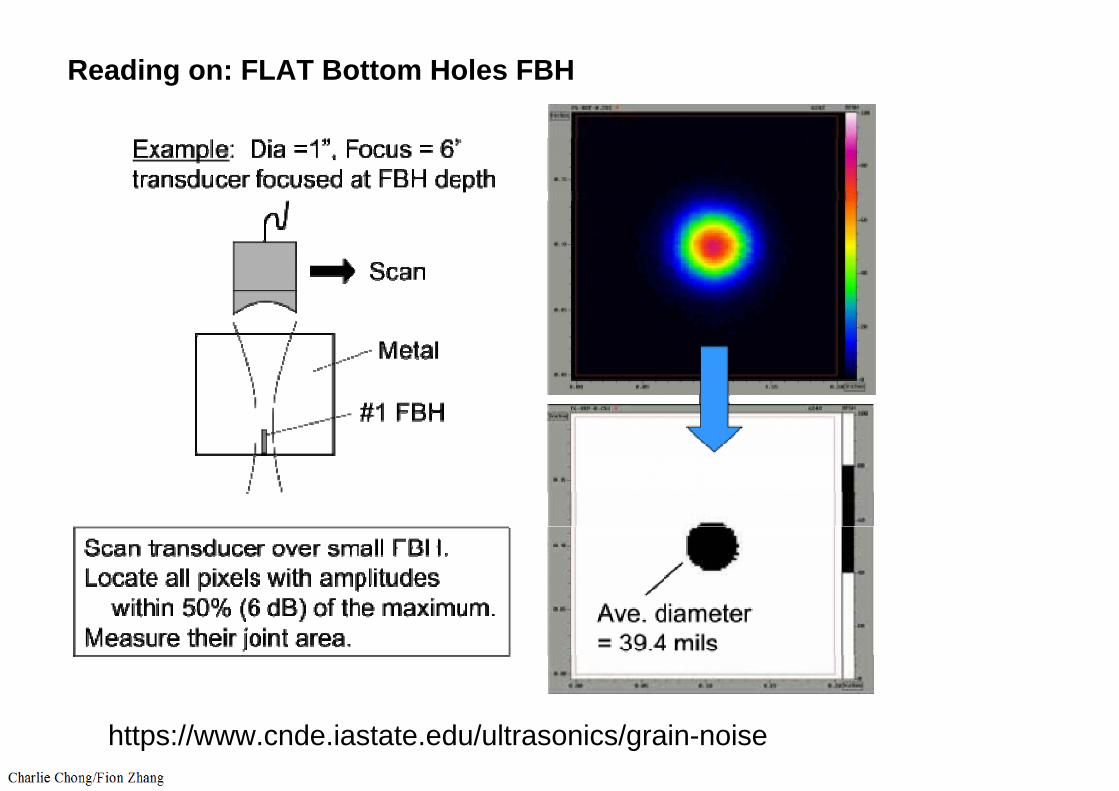
Reading on: FLAT Bottom Holes FBH
https://www.cnde.iastate.edu/ultrasonics/grain-noise

FLAT Bottom Holes FBHA type of reflector commonly used in reference standards. The end (bottom) surface of the hole is the reflector.Equivalent:, the size of a flat-bottom hole which at the same range, gives an ultrasonic indication equal to the one from the discontinuity. This reflector is used in DGS curves, or many calibration blocks, or standards such as the GE specification.
Transfer Corection
Transfer Correction: Reference surface are smooth and scale free unlike the actual work pieces. These call for transfer correction to account for transfer loss resulting from actual scanning.
Transfer Correction: Reference surface are smooth and scale free unlike the actual work pieces. These call for transfer correction to account for transfer loss resulting from actual scanning.

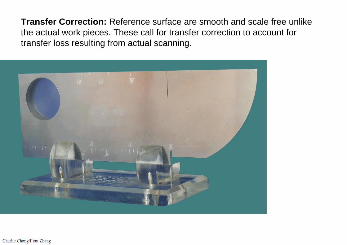
Transfer Correction: Reference surface are smooth and scale free unlike the actual work pieces. These call for transfer correction to account for transfer loss resulting from actual scanning.
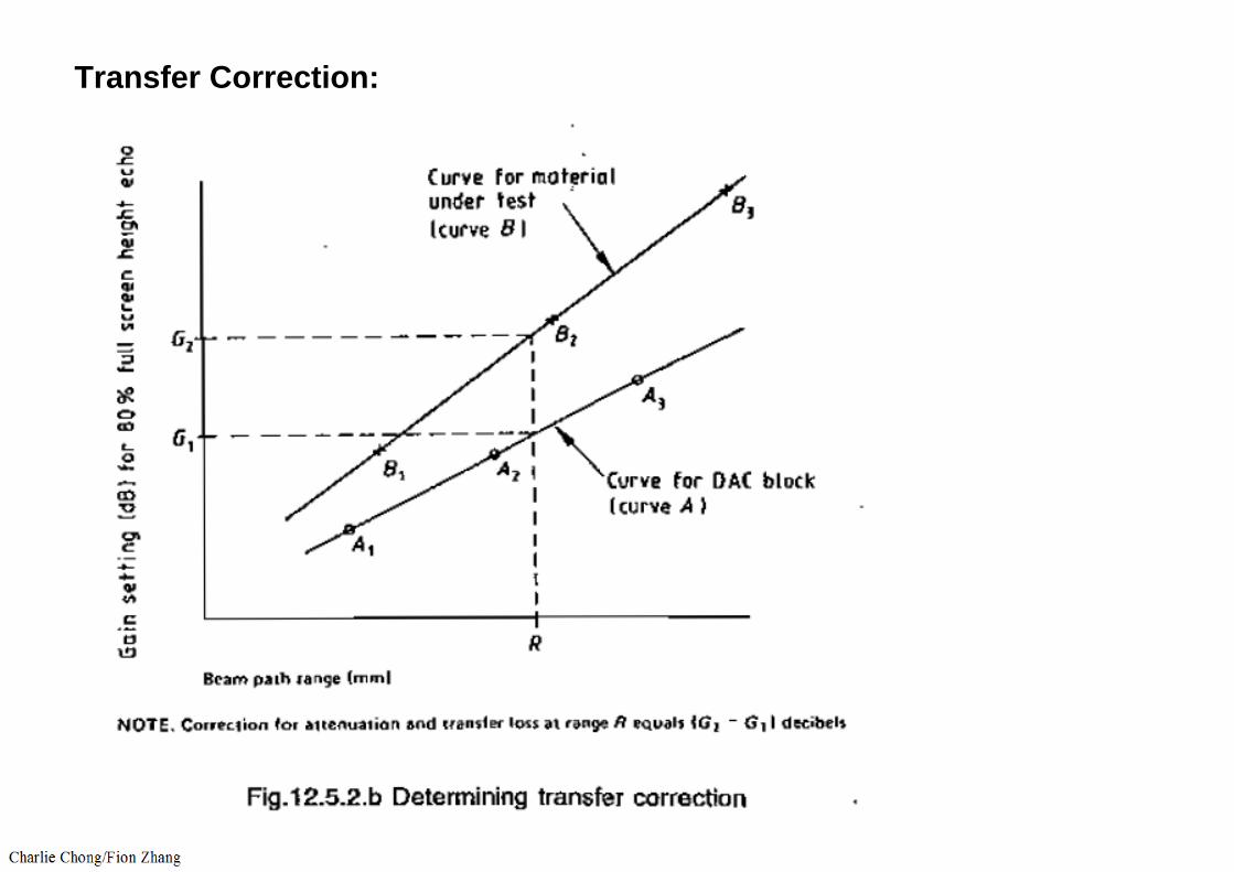
Transfer Correction:
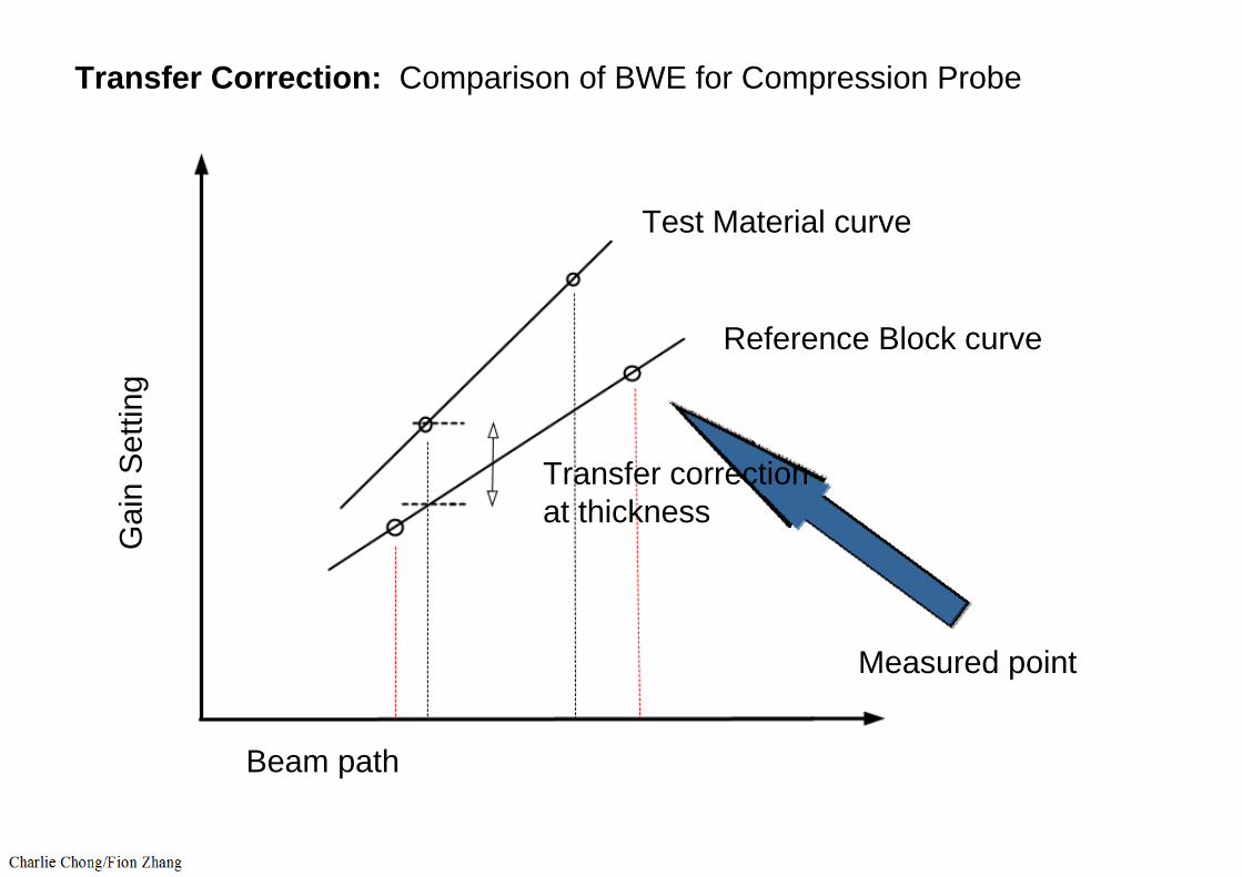
Transfer Correction: Comparison of BWE for Compression ProbeG
ain
Setti
ng
Beam path
Reference Block curve
Test Material curve
Transfer correction at thickness
Measured point

Transfer Correction: Compression Probe Method, Plot a curve of gain setting for FSH at different south paths for actual and reference block, the different in gain control at thickness is the transfer correction.
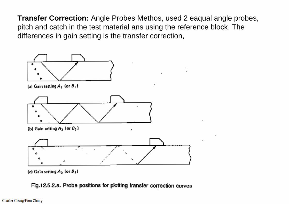
Transfer Correction: Angle Probes Methos, used 2 eaqual angle probes, pitch and catch in the test material ans using the reference block. The differences in gain setting is the transfer correction,
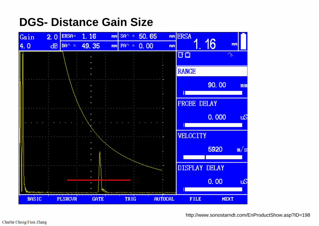
DGS- Distance Gain Size
http://www.sonostarndt.com/EnProductShow.asp?ID=198
FLAT Bottom Holes FBH
■ DGS/AVG
DGS is a sizing technique that relates the amplitude of the echo from a reflector to that of a flat bottom hold at the same depth or distance. This is known as Equivalent Reflector Size or ERS. DGS is an acronym forDistance/Gain/Size and is also known as AVG from its German name, Abstand Verstarkung Grosse. Traditionally this technique involved manually comparing echo amplitudes with printed curves, however contemporary digital flaw detectors can draw the curves following a calibration routine and automatically calculate the ERS of a gated peak. The generated curves are derived from the calculated beam spreading pattern of a given transducer, based on its frequency and element diameter using a single calibration point. Material attenuation and coupling variation in the calibration block and test specimen can be accounted for.
http://www.olympus-ims.com/en/ndt-tutorials/flaw-detection/dgs-avg/
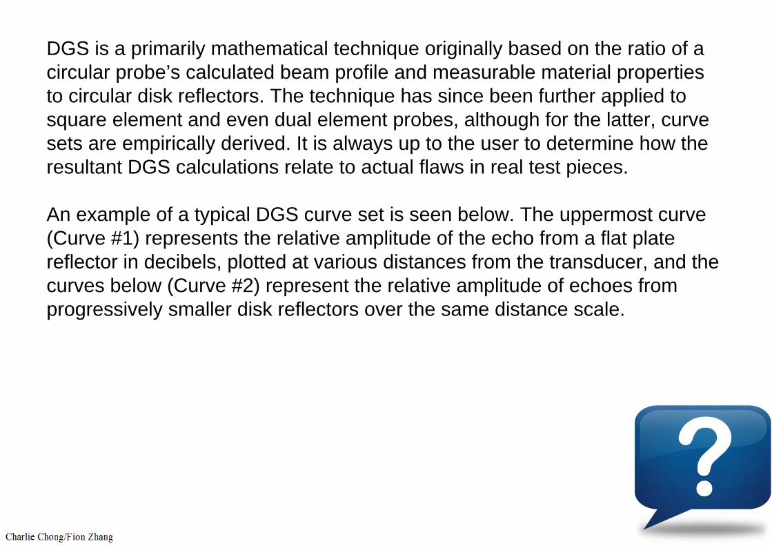
DGS is a primarily mathematical technique originally based on the ratio of a circular probe’s calculated beam profile and measurable material properties to circular disk reflectors. The technique has since been further applied to square element and even dual element probes, although for the latter, curve sets are empirically derived. It is always up to the user to determine how the resultant DGS calculations relate to actual flaws in real test pieces.
An example of a typical DGS curve set is seen below. The uppermost curve (Curve #1) represents the relative amplitude of the echo from a flat plate reflector in decibels, plotted at various distances from the transducer, and the curves below (Curve #2) represent the relative amplitude of echoes from progressively smaller disk reflectors over the same distance scale.
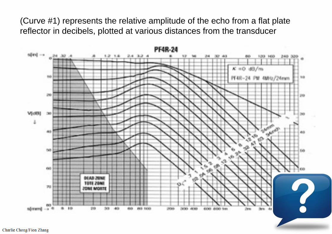
(Curve #1) represents the relative amplitude of the echo from a flat plate reflector in decibels, plotted at various distances from the transducer

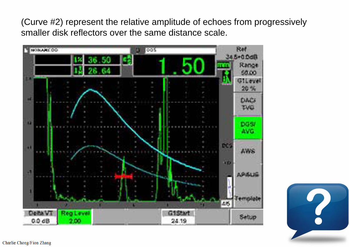
(Curve #2) represent the relative amplitude of echoes from progressively smaller disk reflectors over the same distance scale.

As implemented in contemporary digital flaw detectors, DGS curves are typically plotted based on a reference calibration off a known target such as a backwall reflector or a flat bottom hole at a given depth. From that one calibration point, an entire curve set can be drawn based on probe and material characteristics. Rather than plotting the entire curve set, instruments will typically display one curve based on a selected reflector size (registration level) that can be adjusted by the user. In the example below, the upper curve represents the DGS plot for a 2 mm disk reflector at depths from 10 mm to 50 mm. The lower curve is a reference that has been plotted 6 dB lower.
In the screen at left, the red gate marks the reflection from a 2 mm diameter flat bottom hole at approximately 20 mm depth. Since this reflector equals the selected registration level, the peak matches the curve at that depth. In the screen at right, a different reflector at a depth of approximately 26 mm has been gated. Based on its height and depth in relation to the curve the instrument calculated an ERS of 1.5 mm.
(Curve #2) represent the relative amplitude of echoes from progressively smaller disk reflectors over the same distance scale.
More reading on DGS
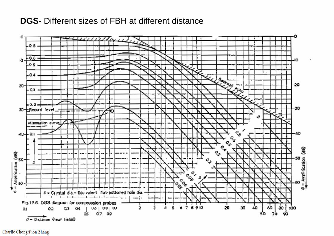
DGS- Different sizes of FBH at different distance

DGS
# of near field

What is DGSTCG is a time-corrected DAC so that equal dimension reflectors give equal amplitude responses for all sound path distances. Used for PAUT Sectorial scans where it would be otherwise impossible to set every angle and sound path to the same sensitivity level using DAC's.
ASTM E-1316: DGS (distance gain size-German AVG) distance amplitude curves permitting prediction of reflector size compared to the response from a back surface reflection.
The probe manufacturer supplies data sheet diagams for each probe which shows the amplitude response curves from the backwall and a range of diameters of flat-bottom holes along the length of the soundfield. Have a look at EN 583-2:2001 Sensitivity and range setting for excellent authoritativedescriptions of DAC/TCG and DGS. You'll have to look at AWS D1.1. for instance for knowledge of their sensitivity setting requirements.Knowledge of these techniques is desirable but will such knowledge really improve your inspection method? You use DAC because the Codes and standards you work to require you to assess indications to those DAC's. A report that a reflector was 3,5 mm equivalent FBH size to DGS would most probably be rejected.
DGS-If you have a signal feom a flaw at a certain depth, you can compare the signal of BWE from the FBH at that depth. The defect then could be sized as equivalent of the size of the FBH.
2.4depth
Size 0.24
Size 0.24
http://www.ndt.net/article/berke/berke_e.htm
Locating & Sizing Flaws

Locating reflectors with an angle-beam probe
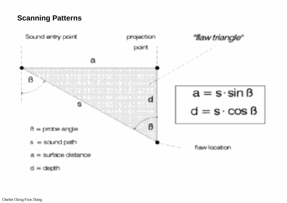
Fig. 53 Scanning a reflector using an angle beam probe The echo of a discontinuity on the instrument display does not now give us any direct information about its position in the material. The only available information for determination of the reflector position is the scale position and therefore the sound path s, this means the distance of the discontinuity from the index point (sound exit point) of the probe, Fig. 53.
The mathematics of the right-angled triangle helps us to evaluate the Surface Distance and the Depth of a reflector which are both important for the ultrasonic test, Fig. 54a. We therefore now have the possibility to instantly mark a detected flaw's position on the surface of the test object by measurement of the surface distance from the sound exit point and to give the depth. For practical reasons, the reduced surface distance is used because this is measured from the front edge of the probe. The difference between the surface distance and the reduced surface distance corresponds to the x-value of the probe, this is the distance of the sound exit point to the front edge of the probe, Fig. 54b.

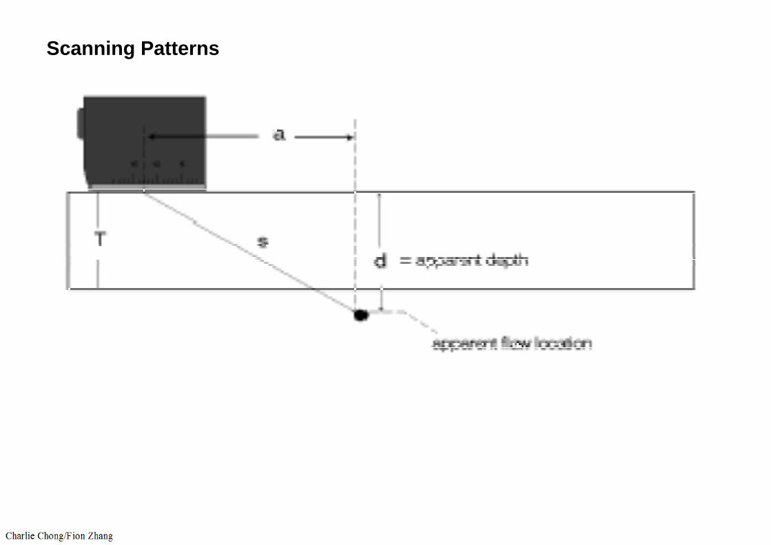
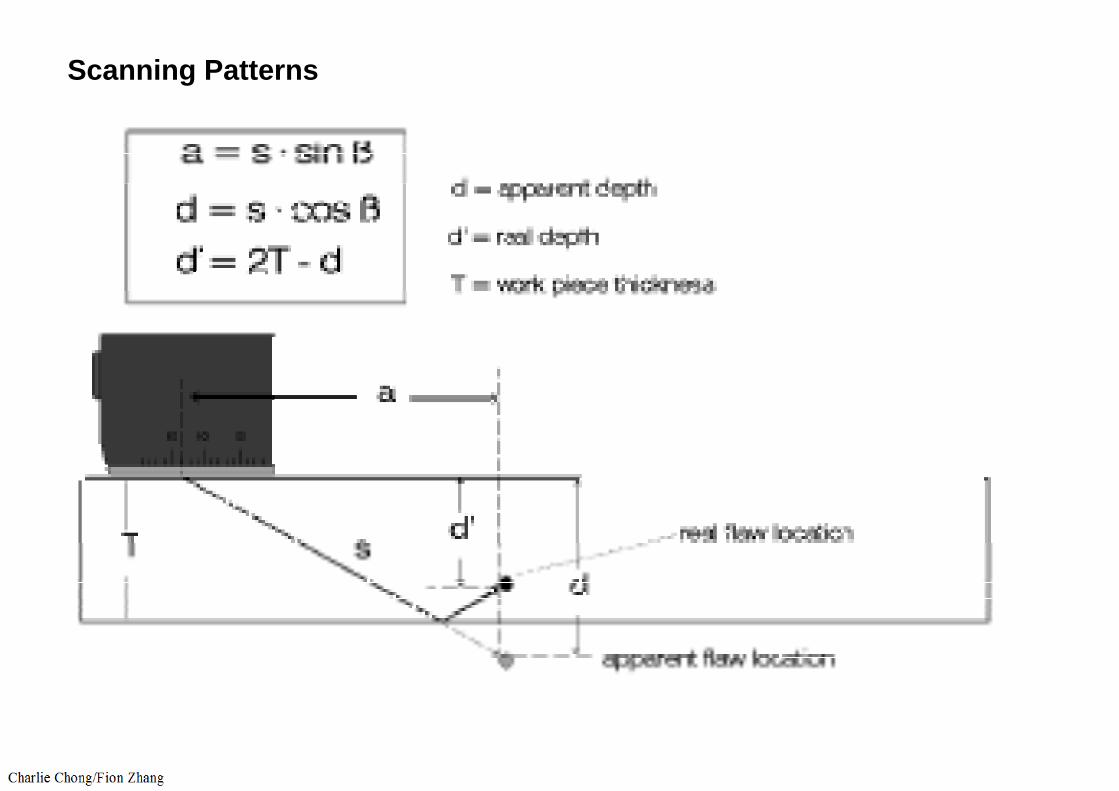
With ultrasonic instruments having digital echo evaluation these calculations are naturally carried out by an integrated microprocessor and immediately displayed so that the operator does not need to make any more time-consuming calculations, Fig. 55. This is of great help with weld testing because with the calculation of the flaw depth an additional factor must be taken into account, namely: whether the sound pulses were reflected from the opposing wall. If this is the case then an apparent depth of the reflector is produced by using the depth formula which is greater than the thickness T of the test object. The ultrasonic operator must acertain whether a reflection comes from the opposite wall and then proceed with calculating the reflector depth, Fig. 56b.

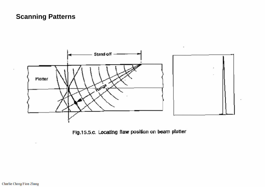
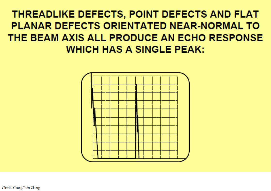
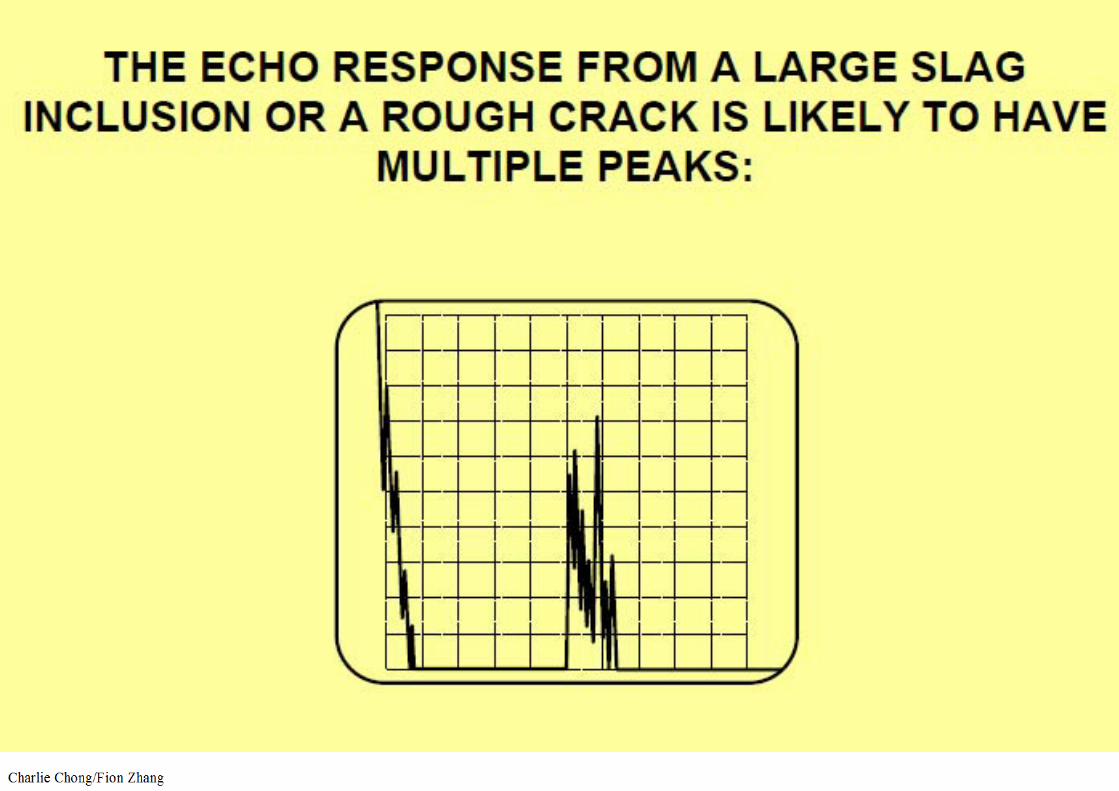
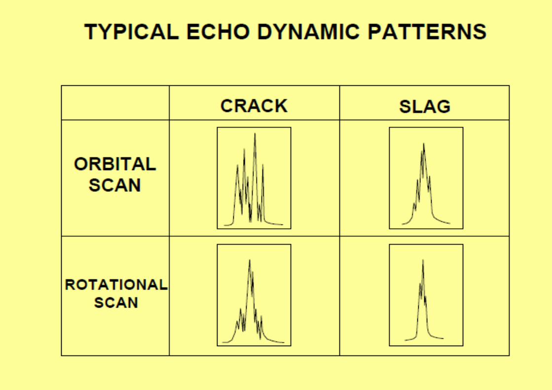
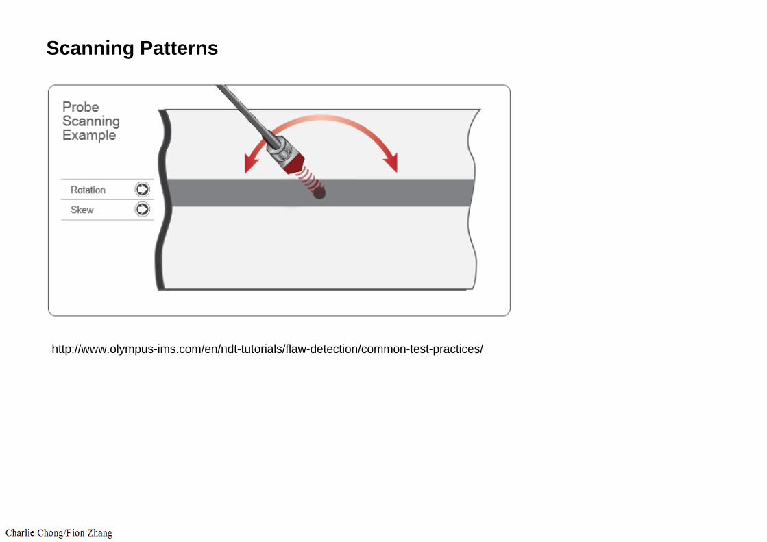
Scanning Patterns
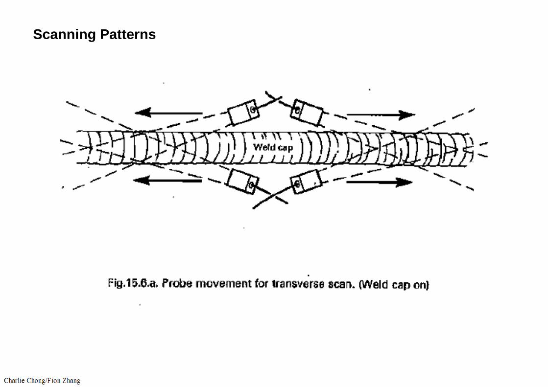
Scanning Patterns

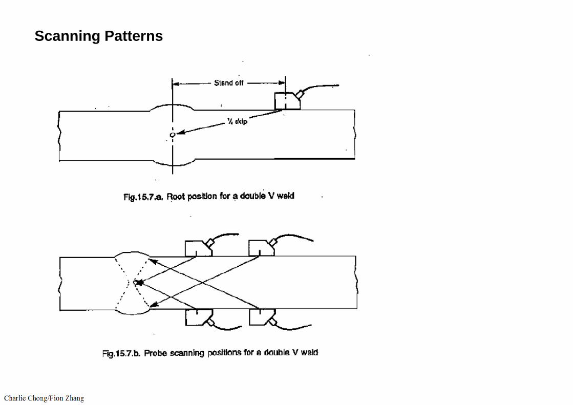
Scanning Patterns
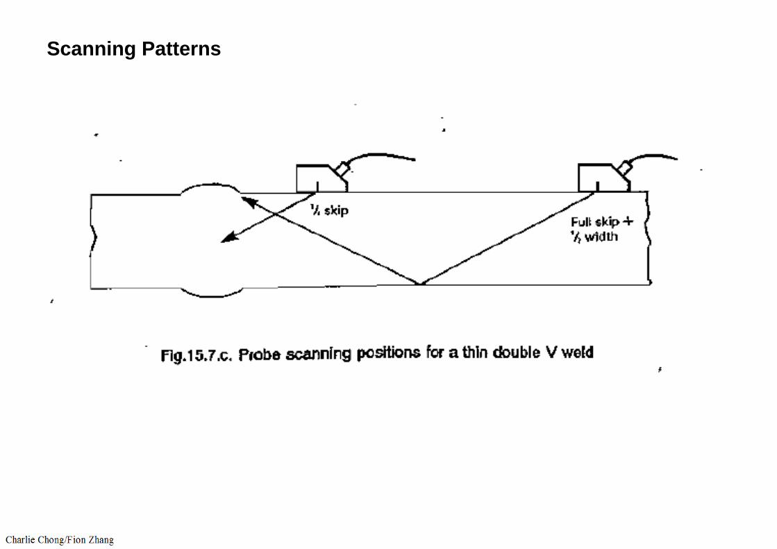
Scanning Patterns
Scanning Patterns

Scanning Patterns
Scanning Patterns

Scanning Patterns

Scanning Patterns
Scanning Patterns
Scanning Patterns
Scanning Patterns

Scanning Patterns
Scanning Patterns
Scanning Patterns

Scanning Patterns
http://www.olympus-ims.com/en/ndt-tutorials/flaw-detection/common-test-practices/
Practice Makes Perfect
81. The 100 mm radius in an IIW block is used to:(a) Calibrate sensitivity level(b) Check resolution(c) Calibrate angle beam distance(d) Check beam angle
80. The 50 mm diameter hole in an IIW block is used to:(a) Determine the beam index point(b) Check resolution(c) Calibrate angle beam distance(d) Check beam angle

Practice Makes Perfect
35. The 2 mm wide notch in the IIW block is used to:(a) Determine beam index point(b) Check resolution(c) Calibrate angle beam distance(d) Check beam angle