Vertical Relationships in the Ready-to-Eat BreakfastCereal Market: A Brand-Supermarket Level Analysis.

By

Benaissa Chidmi, Rigoberto A. Lopez and Ronald W. Cotterill

Selected paper presented at theAmerican Agricultural Economics Association Annual Meetings

Denver, CO-August 1-4, 2004

Vertical Relationships in the Ready-to-Eat Breakfast

Cereal Market: A Brand-Supermarket Level Analysis.

Benaissa Chidmi, Rigoberto A. Lopez, and Ronald W. Cotterill

Abstract: The purpose of this paper is to examine the vertical relationship between the manufacturers of ready-to-eat cereals (RTEC) and the retailers in the Boston area. The study uses highly disaggregated (supermarket and brand level ) monthly data from Information Resources Inc (IRI) from 1995 to 1997.The Logit model is used to estimate the demand for 37 brands of RTEC in the top four supermarkets in the Boston area. The demand estimates are then used to compute the price-cost margins (PCM) for retailers and manufacturers under different vertical scenarios, including vertical Nash double marginalization, non-linear pricing, vertical integration, and collusion. The results of the study shed light on the power each agent (manufacturers and retailers) has to set the price of RTECs in the Boston market, and assess inter- and intra-brand substitution among brands of different manufacturers.

The authors are, respectively, Ph.D. candidate ad professors in the Department of Agricultural and Resource Economics, University of Connecticut, 1376 Storrs Rd., CT 06269. Contact information: R. Lopez, Phone (860) 486-1921, rlopez@canr.uconn.edu. Copyright by B. Chidmi, R.A. Lopez, and R.W. Cotterill. All rights reserved. Readers may make verbatim copies of this document for non-commercial purposes by any means, provided that this copyright notice appears on all such copies.

Vertical Relationships in the Ready-to-Eat Breakfast Cereal

Market: A Brand-Supermarket Level Analysis

1. Introduction

The vertical relationships, including vertical integration and vertical constraints,

between manufacturers and the wholesale and retail firms that distribute their products

are basically the business arrangements between buyers and sellers (Azzam and

Pagoulatos, 1997). Traditionally, vertical relationships have been interpreted either as an

instrument of market power or as a device for correcting failure in the market for

distribution services and improving efficiency. Recently, retailers have become more and

more powerful in negotiating with manufacturers (Villas-Boas, 2002), but it is not

evident whether the manufacturers or the retailers are the chain captains.

The theoretical and institutional aspects of the vertical relationship between

manufacturers and retailers have been much studied in the literature from (McGuire and

Staelin, 1983; Mathewson and Winter, 1984; Rey and Tirole, 1986; Gal-Or, 1991;

Besanko and Perry, 1993; Waterson, 1993; Klein and Murphy 1997; for a survey see

Azzam and Pagoulatos, 1999). The theoretical literature on vertical constraints (resale

price maintenance and exclusive territories) imposed by upstream firms on downstream

firms has focused on the existence of non-linear pricing as a device to internalize the

vertical pricing externality between manufacturers and retailers, and to avoid the double

marginalization problem (Mathewson and Winter, 1984; Rey and Tirole, 1986; Gilligan,

1986; Besanko and Perry, 1993). This literature suggests that for a manufacturing

1

monopoly competition, regulators should not be concerned about vertical restraints as

long as inter-brand competition is not restricted by the contract.

The empirical literature on vertical relationships between manufacturers and

retailers has focused on contracts and vertical integration. Here the emphasis is on

providing a structural model that explains the relationship between manufacturers and

retailers and testing these models using observed data. Some recent and noteworthy

studies in this area are those by Kadiyali et al. (1999), Villas-Boas and Zhao (2000),

Villas-Boas (2002), and Manuszak (2001). In these studies, the quantities and prices are

treated as equilibrium outcomes of some prespecified pricing strategy, generally a

Bertrand-Nash game. These studies use structural models where the demand and supply

relations are estimated using a structural framework.

One important aspect of structured models is that they allow one to study the

manufacturer-retailer relationship without observing wholesale prices and costs at

upstream and downstream levels, which are usually not available as data. The structural

models also allow estimating the mark-ups of manufacturers and retailers.

The ready-to-eat cereal (RTEC) industry along with the supermarket channels in

Boston provides an interesting and useful case study to analyze the vertical relationship

between manufacturers and the retailers. The RTEC industry is characterized by its high

concentration level, high degree of product differentiation, high price-cost margins and

large advertising-to-sales ratios (Schmalensee, 1978; Scherer, 1979; Nevo, 2001).

The fundamental inquiry of this research is to examine the vertical relationship

between manufacturers and retailers in the RTEC industry in Boston in order to shed light

on the power each agent has to set the price of RTECs in the Boston market. More

2

precisely, the question to be answered is: What kind of vertical relationship exists

between the manufacturers and the retailers? Does this relationship support the high

price-cost margins in the RTEC industry? To this end the study uses a discrete choice

model for demand to help estimate the markups at the manufacturer and retailer levels,

and assess the inter- and intra-brand substitution among different manufacturers.

This research will contribute to the existing literature in several ways. First, the

data are highly disaggregated (at the brand and store level) and the variables are monthly

rather than quarterly at the city level used by Nevo (2001). This gives more insight into

the behavior of manufacturers and retailers. Second, the study will add new empirical

evidence on the estimation of the vertical relationship between downstream and upstream

firms. This study differs from Villas-Boas (2002) by looking at retailer strategic behavior,

not at the individual store behavior. Lastly, the study will extend the literature on both the

vertical relationship between manufacturers and retailers and the use of discrete choice to

model consumer demand.

2. The RTEC Industry

The RTEC industry is highly concentrated, with the top four companies

accounting for 84 percent of all RTE cereals. Four companies (Kellogg, General Mills,

Post and Quaker) make practically all of the branded RTE cereal in the United States.

According to Connor (1999), there are 6 to 13 domestic manufacturers of any given

variety of cereal. Production of RTE cereal at the plant level has also become

increasingly concentrated over time (Connor, 1999). In the first decade of the 20th

century, over 100 plants manufactured both hot and cold cereals. During the following 30

years, the number of plants fell dramatically. By 1940, only 30 to 35 plants produced

3

nearly all RTE cereals. The most recent census information indicates that in 1997 36

plants produced all RTE cereals. The dominant cereal manufacturers lower their per unit

production costs by operating large plants that each supply 40 to 60 million pounds of

cereal annually. In addition, the large cereal manufacturers enjoy economies of

advertising.

Because of the high rate of concentration, the major RTEC manufacturers de-

emphasize price competition. In addition to pricing strategies, the major manufacturers

use a variety of nonprice strategies. Advertising is used to differentiate similar cereals

and to create consumer loyalty for particular brands. Connor (1999) shows that the major

branded cereal manufacturers spend 10 to 15 percent of the value of their sales on mass

media advertising. Besides advertising, manufacturers use sales promotions such as

couponing. For RTEC, couponing is the predominant strategy. Companies’ couponing

averages 17 to 20 percent of sales. Nevo and Wolfram (2002) assess the relationship

between coupons and shelf prices in light of the widely expressed view that coupons are

the primary tool for price discrimination. They did not find a relationship between the

coupons and shelf prices.

Top manufacturers of branded RTEC’s produce several brands that cover every

possible segment in the market. This strategy, known as product proliferation, is another

means of competition. Product proliferation also minimizes market penetration by small

firms and private-labels.

Concentration in the RTEC industry was fostered by a wave of mergers in the

1990s. In 1992, General Mills, the second largest U.S. producer of RTEC tried to acquire

the Nabisco cereal line, but later called off the deal for antitrust reasons. The Nabisco

4

cereal line was acquired in 1993 by Kraft, the owner of Post (third largest RTEC

producer) in spite of a challenge by the state of New York; and by the end of 1996

General Mills’s proposal to purchase Ralston Purina’s branded cereal line was approved.

The RTEC industry has also been characterized by high price-cost margins.

According to Nevo (2001), the industry markups are consistent with a Nash-Bertrand

pricing game. The author concludes that the high PCMs are not due to lack of price

competition, but rather to consumer willingness to pay for their favorite brand and pricing

decisions by firms that take into account limited substitution among their own brands.

Thus market power, if any, in this industry is due to the firm’s ability to maintain a

portfolio of differentiated products and influence perceived product quality through

advertising.

3. The Model

Following Villas-Boas (2002), this paper examines the vertical

relationship between the RTEC manufacturers and the supermarkets in Boston at the

supermarket chain level. Three categories of scenarios are examined, assuming a vertical

Nash behavior: (1) double marginalization pricing; (2) non-linear pricing behavior; and

(3) collusive pricing behavior. This task depends on the estimated demand functions of

RTEC brands in the market under study, estimated using a discrete choice method.

3.1. Demand Side

Consider a consumer choosing N brands sold by J retailers during each

shopping trip at time t. The indirect utility of consumer from buying the brand i j during

the travel trip is given by t

5

ijtjtjtiijtjijt pxU εζαββ ++−+=

j

, (1)

where β represents the store fixed effects, are the observed product characteristics,

is the price of brand

jtx

jtp j , jtζ are the unobserved (by the econometrician) product

characteristics, and jtiε represents the distribution of consumer preferences about the

unobserved product characteristics with a distribution density )(εf . The parameters to

be estimated are iα and iβ . Note that those parameters are allowed to vary across

consumers, therefore allowing random coefficients for consumers’ preferences. These

random coefficients can be decomposed into a fixed component not varying across

consumers, and a varying component changing according to observed and unobserved

consumer characteristics. That is,

iii vD γλαα ++= , (2)

iii vD γλββ ++=

iD

iv

, (3)

where the represents observed consumers characteristics (such as demographics,

income) and represents unobserved consumers characteristics. Substituting equations

(2) and (3) into (1) yields

ijtjtjtijtijtjtijtijtjijt pvpDpxvxDxU εζγλαγλββ ++−−−+++= . (4)

Assume that the unobserved consumer characteristics v are normally distributed ,

and the observed consumer characteristics have an empirical distribution h from

the demographic data.

i ),0( IN

iD )(D

The indirect utility given in equation (4) consists of two parts: a mean utility

given by jtjtjtjjt px ζαββδ +−+= and a deviation from that mean, which is a function

6

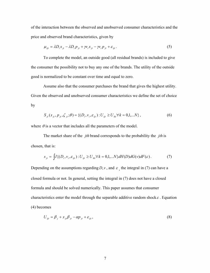
of the interaction between the observed and unobserved consumer characteristics and the

price and observed brand characteristics, given by

ijtjtijtijtijtiijt pvxvpDxD εγγλλµ +−+−= . (5)

To complete the model, an outside good (all residual brands) is included to give

the consumer the possibility not to buy any one of the brands. The utility of the outside

good is normalized to be constant over time and equal to zero.

Assume also that the consumer purchases the brand that gives the highest utility.

Given the observed and unobserved consumer characteristics we define the set of choice

by

},...1,0:),,{();,,( NkUUvDpxS iktijtijtiijtjtjtjt =∀≥= εθζ , (6)

where θ is a vector that includes all the parameters of the model.

The market share of the brand corresponds to the probability the is

chosen, that is:

jth jth

)()()(},...1,0:),,{( εε dFvdGDdHNkUUvDIs iktijtijtiijt ∫ =∀≥= . (7)

Depending on the assumptions regarding , and vD, ε , the integral in (7) can have a

closed formula or not. In general, setting the integral in (7) does not have a closed

formula and should be solved numerically. This paper assumes that consumer

characteristics enter the model through the separable additive random shockε . Equation

(4) becomes

ijtjtjtjtjijt pxU εαββ +−+= , (8)

7

which corresponds to the logit model. In this situation the integral in equation (7) has a

closed form and can be solved analytically. The brand market shares are given by the

following equation:

∑=

−+

−= J

kktkt

jtjtjt

px

pxs

1

)exp(1

)exp(

α

αβ. (9)

The market shares defined by equation (9) give the following price elasticities:

)1( jtjtjt

kt

kt

jtjkt sp

sp

ps

−=∂

∂= αη , for kj = ; and (10)

ktjtjt

kt

kt

jtjkt sp

sp

ps

αη =∂

∂= , otherwise.

3.2. Supply Side

In this section, the scenarios considered are described, and the corresponding

models are solved to obtain the retailers’ and the manufacturers’ price cost margins. All

models assume vertical Nash pricing. In addition, pricing is assumed to be a two-stage

game. First, the manufacturers choose the wholesale prices to their retailers. Then, the

retailers choose the retail prices to maximize their own profits, given the wholesale prices

and their incurred costs. The game is solved using backward induction starting from the

retailers and going back to the manufacturers’ equilibrium.

3.2.1. Double Marginalization Scenario

Beginning with the retail problem, consider that there are Bertrand-Nash

retailers in the retail market, and Bertrand-Nash manufacturers competing in the

wholesale market. The rth retailer’s problem is to maximize profit, given by

rN

wN

8

)()( pscwp jtrjtjt

Sjjtrt

rt

−−= ∑∈

π , (11)

where is the set of brands sold by the rth retailer at time t, is the wholesale price

the retailer pays for brand

rtS jtw

rth j , is the retailer’s marginal cost for brand rjtc j , is

the share of brand

)( ps jt

j , and M is a measure of the market size. This measure is assumed to

be proportional to the population of the market under study. The first order conditions are

given by

0)( =∂∂

−−+ ∑∈ jt

mtrmtmt

Smmtjt p

scwps

rt

. (12)

Repeating the same procedure for each retailer and each brand and stacking all the first

order conditions together, we get the following implied price cost margin as a function of

the demand side:

)()*( 1 psTcwp trtrrttt

−∆−=−− , (13)

where T is the retailer’s ownership matrix with the general element T equal to one

when the brands and

r ),( jir

i j are sold by the same retailer and zero otherwise; and ∆ is a

matrix of first derivatives of all the shares with respect to all retail prices. The matrix

is the element by element multiplication of the two matrices.

rt

)rt*( rT ∆

Turning now to the upstream level, each manufacturer sets the wholesale price

in order to maximize profit, given by w

))(()( wpscw jtwjt

Sjjtwt

wt

−= ∑∈

π , (14)

9

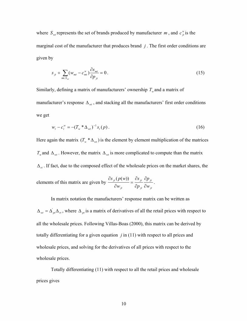
where represents the set of brands produced by manufacturer , and is the

marginal cost of the manufacturer that produces brand

wtS m wjtc

j . The first order conditions are

given by

0)( =∂∂

−+ ∑∈ jt

mtwmt

Smmtjt p

scws

wt

. (15)

Similarly, defining a matrix of manufacturers’ ownership and a matrix of

manufacturer’s response , and stacking all the manufacturers’ first order conditions

we get

wT

wt∆

)()*( 1 psTcw twtwwtt

−∆−=− . (16)

Here again the matrix ( is the element by element multiplication of the matrices

and . However, the matrix

)* wtwT ∆

wT wt∆ wt∆ is more complicated to compute than the matrix

. If fact, due to the composed effect of the wholesale prices on the market shares, the

elements of this matrix are given by

rt∆

jt

jt

jt

jt

jt

jt

wp

ps

wwps

∂

∂

∂

∂=

∂

∂ ))((.

In matrix notation the manufacturers’ response matrix can be written as

, where is a matrix of derivatives of all the retail prices with respect to

all the wholesale prices. Following Villas-Boas (2000), this matrix can be derived by

totally differentiating for a given equation

rtptwt ∆∆=∆ 'pt∆

j in (11) with respect to all prices and

wholesale prices, and solving for the derivatives of all prices with respect to the

wholesale prices.

Totally differentiating (11) with respect to all the retail prices and wholesale

prices gives

10

0),(]),())(),(([2

11=

∂

∂−

∂∂

+−−∂∂

∂+

∂

∂∑∑==

fj

frk

j

kr

riii

kj

iN

ir

N

k k

j dwps

jfTdpps

jkTcwppp

sjiT

ps

.

(17)

In matrix notation, (17) becomes

0=− ff dwHGdp . (18)

Solving for the derivatives of all prices with respect to the wholesale prices gives

ff

HGdwdp 1−= . (19)

Therefore

∆ . (20) fp HG 1−=

Finally, the implied price-cost margins for the retailers and the manufacturers is

obtained by summing up the implied price-cost margin for the retailer and the price-cost

margin for the manufacturer of equations (12) and (15)

)()*()()*( 11 psTpsTccp twtwtrtrwt

rtt

−− ∆−∆−=−− . (21)

3.2.2. Non-Linear Pricing Scenario

The Non-linear pricing occurs when the manufacturer sets the price equal to

marginal cost and lets the retailer be the residual claimant. The retailers pay the

manufacturer part or the full surplus in the form of a fixed fee, depending on the power

they have. In a one manufacturer-one retailer case, this pricing model (known as a two-

part tariff) is optimal under a demand certainty assumption (Tirole, 1988, page 176) when

the retailers follow manufacturers in setting prices. Rey and Tirole (1986) and Tirole

11

(1988, page 177) have shown that the two-part tariff is still optimal in the simple double

marginalization setting under demand uncertainty and asymmetric information.

In the case of multiple manufacturers and multiple retailers, the non-linear pricing

model can be analyzed under two different sub-cases. In the first sub-case, one can

assume that the manufacturers’ margins are zero. Given that the wholesale prices are

equal to marginal costs, the retailers have the ultimate decision in setting prices. In the

second sub-case, the retailers’ margins are assumed to be zero, in which case the

manufacturers have the pricing decision and set the final consumer prices. In either case,

one agent is exercising market power by setting the price well above marginal costs, and

the channel’s profits will be higher than in the case of double marginalization.

Case 1: Manufacturers margins are zero

In this case the manufacturers’ implied price-cost margins are zero and the

wholesale prices are equal to marginal costs. The implied price-cost margins for the

retailers are given by replacing the wholesale prices by the marginal costs ( ).

Hence equation (12) becomes

wtt cw =

)()*( 1 psTccp trtrwt

rtt

−∆−=−− . (22)

This scenario gives the retailers the entire margin of the industry and implies a more

vertically integrated structure at the retail level.

Case 2: Retailers margins are zero

In this case the retailers’ implied price-cost margins are set to zero, and the final

price the consumers pay is the sum of the wholesale price and the retailers’ marginal

costs, i.e., . The manufacturers get all the channel’s profits. Their implied rjtjtjt cwp +=

12

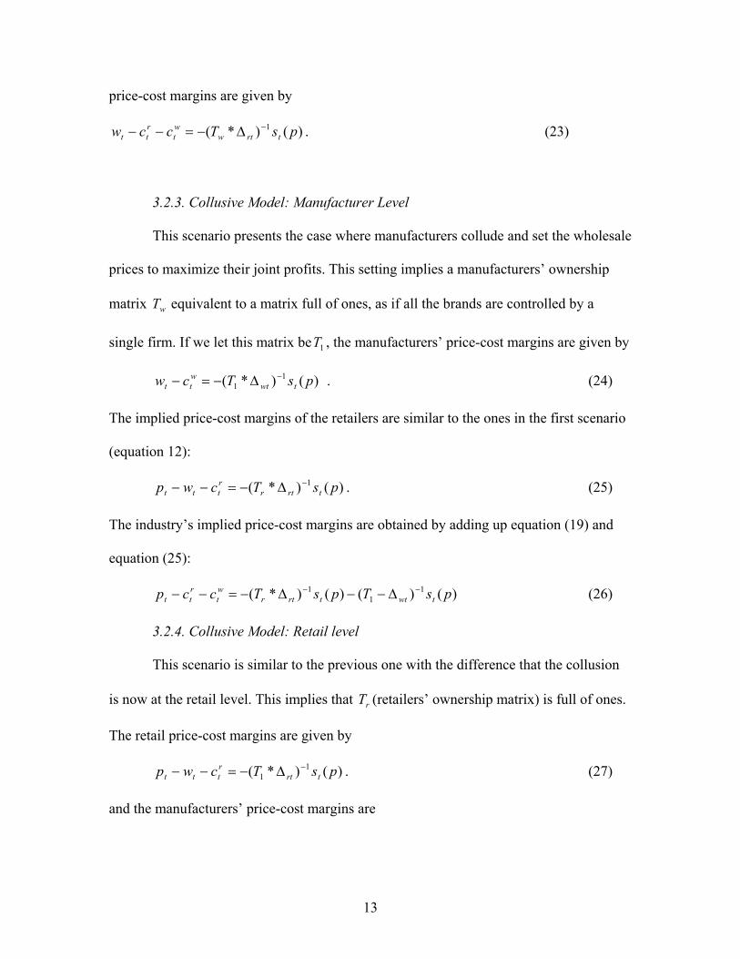
price-cost margins are given by

. (23) )()*( 1 psTccw trtwwt

rtt

−∆−=−−

w

()*( 11 sTcw twt

wtt

−∆−=−

)*(Tcwp rtrrttt

−∆−=−−

)*(Tccp rtrwt

rtt

−∆−=−−

)*( 1Tcwp rtrttt

−∆−=−−

3.2.3. Collusive Model: Manufacturer Level

This scenario presents the case where manufacturers collude and set the wholesale

prices to maximize their joint profits. This setting implies a manufacturers’ ownership

matrix T equivalent to a matrix full of ones, as if all the brands are controlled by a

single firm. If we let this matrix beT , the manufacturers’ price-cost margins are given by 1

) . (24) p

The implied price-cost margins of the retailers are similar to the ones in the first scenario

(equation 12):

)(1 pst . (25)

The industry’s implied price-cost margins are obtained by adding up equation (19) and

equation (25):

)()()( 11

1 psTps twtt−∆−− (26)

3.2.4. Collusive Model: Retail level

This scenario is similar to the previous one with the difference that the collusion

is now at the retail level. This implies that T (retailers’ ownership matrix) is full of ones.

The retail price-cost margins are given by

r

)(1 pst . (27)

and the manufacturers’ price-cost margins are

13

)()*( 1 psTcw twtwwtt

−∆−=− . (28)

Adding up (27) and (28) gives the industry implied price-cost margins

)()()()*( 111 psTpsTccp twtwtrt

wt

rtt

−− ∆−−∆−=−− . (29)

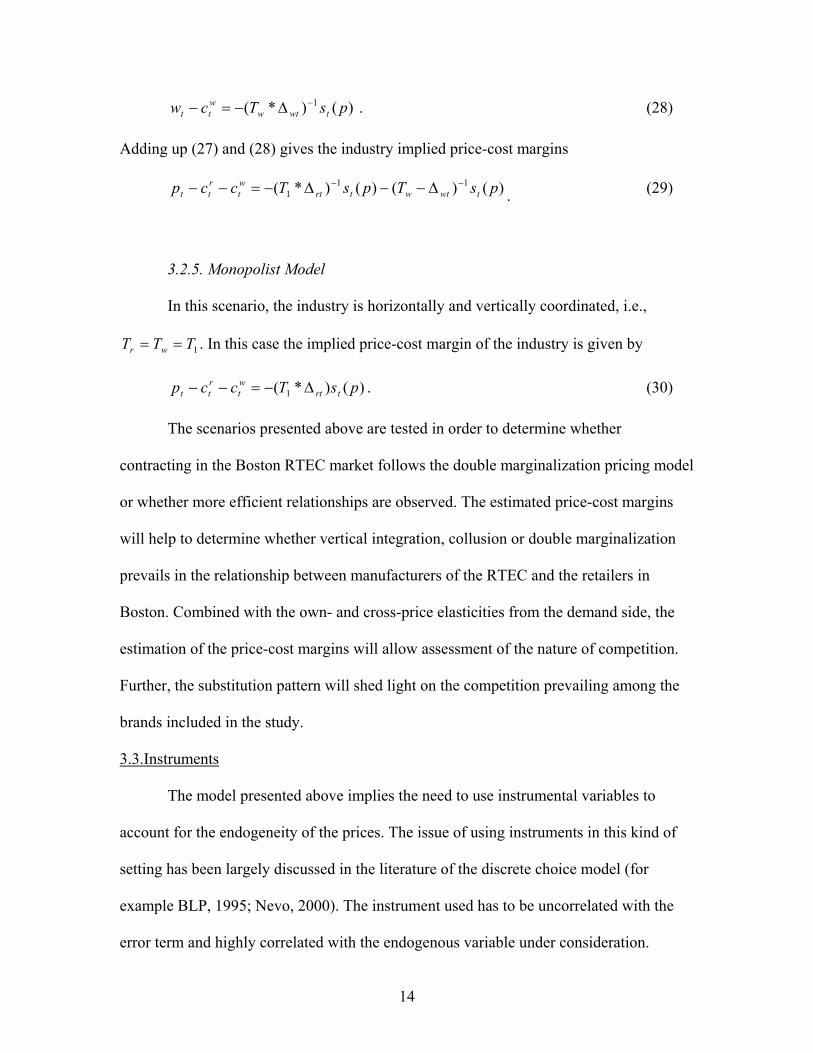
3.2.5. Monopolist Model

In this scenario, the industry is horizontally and vertically coordinated, i.e.,

. In this case the implied price-cost margin of the industry is given by 1TTT wr ==

)()*( 1 psTccp trtwt

rtt ∆−=−− . (30)

The scenarios presented above are tested in order to determine whether

contracting in the Boston RTEC market follows the double marginalization pricing model

or whether more efficient relationships are observed. The estimated price-cost margins

will help to determine whether vertical integration, collusion or double marginalization

prevails in the relationship between manufacturers of the RTEC and the retailers in

Boston. Combined with the own- and cross-price elasticities from the demand side, the

estimation of the price-cost margins will allow assessment of the nature of competition.

Further, the substitution pattern will shed light on the competition prevailing among the

brands included in the study.

3.3.Instruments

The model presented above implies the need to use instrumental variables to

account for the endogeneity of the prices. The issue of using instruments in this kind of

setting has been largely discussed in the literature of the discrete choice model (for

example BLP, 1995; Nevo, 2000). The instrument used has to be uncorrelated with the

error term and highly correlated with the endogenous variable under consideration.

14

BLP(1995) note that if the producers know the values of the unobserved (to the

econometrician) characteristics, then the prices are likely to be correlated with them. For

the automobile industry they suggest using the cost and demand characteristics for all

products in a given year. Nevo (2000) uses two alternative sets of instrumental variables:

the prices of the brand in other cities and a set of instruments that attempt to proxy for

regional marginal costs (material, labor, energy, transportation). Villas-Boas (2002) uses

the interactions between the input prices and the brand dummy variables. This study

considers two sets of instrumental variables: the prices of the brand in other markets

(supermarkets) and the product characteristics of the brands. The use of the other prices

as instruments comes from the fact that for a given brand, the manufacturer is unique and

the wholesale prices charged for different retailers would be comparable. As argued by

BLP (1995), the product characteristics are correlated with their prices.

4. Data Sources and Management

The study is conducted using a scanner data set from Information Resources Inc

(IRI) that covers purchases of RTEC in four supermarkets in Boston (Stop & Shop,

Shaw’s, Demoulas and Star Market) by unit sales, volume sales, dollar sales, percentage

of RTE cereals sold under any type of merchandising, and the weighted average of any

price reduction. The data are for four-week periods from February 1995 to December

1997. Prices are computed using volume sales and dollar sales. Market shares are

computed using volume sales (converted to servings, one serving equal to 30 gr) and the

market size. The market size corresponds to the potential market obtained by multiplying

the total population in the Boston market by the per capita monthly consumption of RTE.

5. Results

15

5.1. Logit Demand

Table 1 presents the results of the regression of )ln()ln( 0tjt ss − on prices,

promotion and product characteristics. The characteristics included are the content of

calories, sugar, proteins, vitamins, minerals, sodium, potassium, fiber and total fat. The

regression also includes dummy variables for corn, oat, rice and fruits and a dummy

variable for children’s cereals.

Table 1 Logit Results.

Variables OLS Estimates IV Estimates

Price -9.9046*** (0.2795) -11.9629*** (3.0531)

Promotion 0.0078*** (0.0004) 0.0070** (0.0025)

Calories -0.0179*** (0.0008) -0.0163*** (0.0054)

Total Fat 0.0298* (0.0185) 0.0583 (0.1267)

Sugar -0.0207*** (0.0034) -0.0149 (0.0235)

Proteins 0.1316*** (0.0136) 0.1371* (0.0903)

Fiber -0.0291** (0.0146) -0.0562 (0.1018)

Minerals 0.0009 (0.0017) -0.0019 (0.0119)

Vitamins -0.0165*** (0.0013) -0.0114 (0.0103)

Sodium -0.0030*** (0.0003) -0.0021 (0.0019)

Potassium 0.0037*** (0.0003) 0.0030 (0.0021)

Corn Dummy 0.0243 (0.0361) 0.0468 (0.2397)

Oat Dummy 0.2365*** (0.0347) 0.1589 (0.2466)

Rice Dummy 0.0644 (0.0530) 0.0351 (0.3517)

Fruit Dummy 0.1301***(0.0250) 0.0926 (0.1712)

Kid Dummy -0.3680*** (0.0306) -0.2773 (0.2287)

Figures in parentheses are the standard deviations of the estimates. (***) Significant at 0.1% level. (**) Significant at 5% level. (*) Significant at 10% level.

16

The second column of Table 1 presents the results of the ordinary least squares

(OLS) regression, while column 3 presents the instrumental variables (IV) results of a

two-stage least squares regression. For each brand, the IVs are obtained by stacking

together the product characteristics and the price of the same brand in the other stores.

The OLS and IV results show that most of the variables are of the expected sign with few

exceptions. Hence, the parameter estimates of the price, calories, sugar and sodium are

negative as one would expect. On other hand, the parameter estimates of proteins,

minerals and potassium are positive as expected. However, one does not expect total fat

to have a positive effect on the share of the brand, nor the fiber and vitamins contents to

have a negative effect. The negative sign of fat content may be explained by the fact that

RTECs are not a major source of fat and consumers do not have this concern when they

chose their brand.

Table 2 gives the own-price elasticities estimated from the Logit model as given

in equation (10). As expected, all the own-price elasticities are negative with a magnitude

greater than one in absolute value. This implies that at the supermarket level the demand

for differentiated brands is elastic. The elasticities range from -3.2556 to -1.7889 in the

Stop & Shop supermarket channels, for Shaw’s, from -3.4691 to -2.1770, while for

Demoulas and Star Market the elasticites range from -3.4393 to -1.9683 and from -3.4156

to -2.2650 respectively. These elasticities are comparable to those found by Nevo (2001)

taking into account consumer heterogeneity. From the results it appears that the same

brand has different elasticity values in different supermarket channels. Furthermore, for

almost all brands included in the study, the brands’ demand is less elastic in the Stop &

Shop supermarket channel than in other channels.

17

At the manufacturer level the elasticities range from -3.2198 for General Mills

Cheerios to -2.3636 for Quaker Oat. On average, the own-price elasticities are higher (in

absolute value) for General Mills brands than for Kellogg, Post, Quaker and Nabisco

brands.

To analyze the substitution pattern between different brands, Table 3 gives the

cross-price elasticities for some selected brands of Kellogg and General Mills in the Stop

& Shop supermarket channel.

Table 2 Own-Price Elasticities by Brand and Market Channel

Stop & shop Shaws Demoulas Star Market ManufacturerGM Cheerios -2.8288 -3.2219 -3.4373 -3.3911 -3.2198 GM CinnamonTSTCrunch -2.6433 -3.2598 -3.4393 -3.2408 -3.1458 GM CocoaPuffs -2.6301 -3.2375 -2.6674 -3.3354 -2.9676 GM GoldenGrahams -2.5747 -3.22 -2.4447 -3.4156 -2.9138 GM HoneyNutCheerios -2.1433 -3.2302 -3.3597 -2.5593 -2.8231 GM Kix -2.6587 -3.2334 -3.3586 -3.3595 -3.1526 GM LuckyCharms -2.5449 -3.2157 -3.0487 -3.3053 -3.0287 GM MultiGrainCheerios -2.6045 -3.1783 -3.0424 -3.2759 -3.0253 GM Total -2.4665 -2.1823 -2.4375 -3.2917 -2.5945 GM TotalRaisinBran -2.1638 -3.2082 -2.9995 -2.5683 -2.7350 GM Wheaties -1.7889 -3.0579 -3.0329 -3.059 -2.7347 GM AppleCinnamonCheers -2.0625 -3.0742 -2.9756 -3.3345 -2.8617 K AppleJacks -2.3848 -3.0823 -2.7519 -2.7525 -2.7429 K CompleteBranFlakes -2.5469 -2.6375 -2.2352 -3.2215 -2.6603 K CornFlakes -1.8332 -2.9903 -2.5755 -2.9821 -2.5953 K CornPops -2.3094 -2.9122 -2.6035 -3.1738 -2.7497 K Crispix -2.4271 -2.2038 -2.6106 -2.8279 -2.5174 K FrootLoops -2.0428 -2.8221 -2.5868 -2.8608 -2.5781 K FrostedFlakes -2.0809 -2.7905 -2.7079 -2.9187 -2.6245 K FrostedMiniWheats -2.0747 -2.177 -2.7078 -3.0023 -2.4905 K RaisinBran -2.2567 -2.5723 -2.6528 -2.679 -2.5402 K RiceKrispies -2.25 -2.4863 -2.6617 -2.8295 -2.5569 K SpecialK -2.1384 -2.715 -2.6258 -2.7031 -2.5456 P BananaNutCrunch -2.2757 -2.4598 -2.4678 -2.668 -2.4678 P CocoaPebbles -1.9473 -2.6492 -2.4345 -2.8006 -2.4579 P FruitPebbles -2.2658 -2.6249 -2.3862 -2.7162 -2.4983 P GrapeNuts -2.2602 -2.6467 -2.3484 -2.8862 -2.5354 P HoneyComb -2.1867 -2.5998 -2.2358 -2.9675 -2.4975 P RaisinBran -2.164 -2.6581 -2.2092 -3.1005 -2.5330 Q Life -2.2005 -2.6573 -2.0236 -2.7298 -2.4028 Q Oat -2.1417 -2.5711 -1.9683 -2.7734 -2.3636 Q Toasted -2.0853 -2.2152 -3.3101 -2.724 -2.5837

18

N FrostedWheatBites -1.9361 -2.6009 -3.1923 -2.6987 -2.6070 N SpoonSize -1.8806 -3.4691 -3.3072 -2.265 -2.7305 R CookieCrisp -1.9843 -3.4647 -3.2158 -2.7783 -2.8608 R CornChex -3.2556 -3.4512 -3.194 -2.7735 -3.1686 R RiceChex -3.227 -3.4339 -3.2095 -2.8035 -3.1685

Table 3 Own- and Cross-Price Elasticities for Selected Brands in Stop & Shoe Supermarket Channel.

GM Cheerios

GM Golden Graham

GM Kix GM Total

K Corn Flakes

K Frosted Flakes

K rice Krispies

GM Cheerios -2.8288 0.0103 0.0179 0.0193 0.0146 0.0180 0.0223GM Golden Graham 0.0299 -2.5747 0.0236 0.0255 0.0192 0.0237 0.0294GM Kix 0.0289 0.0132 -2.6587 0.0245 0.0185 0.0229 0.0283GM Total 0.0295 0.0135 0.0233 -2.4665 0.0190 0.0234 0.0290K Corn Flakes 0.0148 0.0067 0.0117 0.0126 -1.8332 0.0117 0.0145K Frosted Flakes 0.0209 0.0095 0.0165 0.0177 0.0134 -2.0809 0.0205K Rice Krispies 0.0256 0.0117 0.0202 0.0218 0.0165 0.0203 -2.2500

Note that all the cross-price elasticities are positive, meaning that the brands are

substitutes of each other. However, these elasticities do not give a clear substitution

pattern between brands due to the restrictive and unrealistic substitution pattern implied

by the Logit model.

5.2. Price-Cost Margins

Given the demand parameters estimated, we can use scenarios previously

described to compute PCM for different brands and market channels. Summary statistics

for the PCM estimates, given a Logit demand model, are provided in table 4. For the

double marginalization model the retail margins are higher than the wholesale or

manufacturer margins. Manufacturer margins average 53% when the manufacturer

19

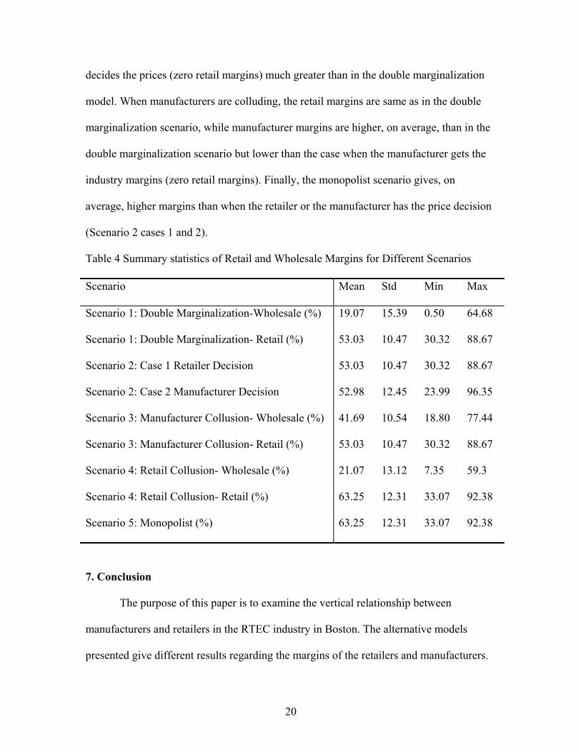
decides the prices (zero retail margins) much greater than in the double marginalization

model. When manufacturers are colluding, the retail margins are same as in the double

marginalization scenario, while manufacturer margins are higher, on average, than in the

double marginalization scenario but lower than the case when the manufacturer gets the

industry margins (zero retail margins). Finally, the monopolist scenario gives, on

average, higher margins than when the retailer or the manufacturer has the price decision

(Scenario 2 cases 1 and 2).

Table 4 Summary statistics of Retail and Wholesale Margins for Different Scenarios

Scenario Mean Std Min Max

Scenario 1: Double Marginalization-Wholesale (%) 19.07 15.39 0.50 64.68

Scenario 1: Double Marginalization- Retail (%) 53.03 10.47 30.32 88.67

Scenario 2: Case 1 Retailer Decision 53.03 10.47 30.32 88.67

Scenario 2: Case 2 Manufacturer Decision 52.98 12.45 23.99 96.35

Scenario 3: Manufacturer Collusion- Wholesale (%) 41.69 10.54 18.80 77.44

Scenario 3: Manufacturer Collusion- Retail (%) 53.03 10.47 30.32 88.67

Scenario 4: Retail Collusion- Wholesale (%) 21.07 13.12 7.35 59.3

Scenario 4: Retail Collusion- Retail (%) 63.25 12.31 33.07 92.38

Scenario 5: Monopolist (%) 63.25 12.31 33.07 92.38

7. Conclusion

The purpose of this paper is to examine the vertical relationship between

manufacturers and retailers in the RTEC industry in Boston. The alternative models

presented give different results regarding the margins of the retailers and manufacturers.

20

The paper follows the approach that consists of determining the PCMs of the agents

(retailers and manufacturers) without observing the wholesale prices. This approach

relies heavily on the choice of the demand estimation method. This paper uses the Logit

model to estimate the parameters of the demand for RTECs in the Boston market. Given

demand estimates, the PCMs implied by different vertical contracting between retailers

and manufacturers are estimated. The results show that the double marginalization

scenario does not give the highest margins to manufacturers and retailers. In the double

marginalization setting, retailers’ margins are greater than manufacturers’ margins. This

may suggest that retailers are the chain captains. When manufacturers collude, citerus

paribus their margin increases and the industry margin increases making the consumer

take the burden of the collusion. When the retailers collude, citerus paribus their margin

increases compared to double marginalization and here again the consumer is paying the

cost of retailers’ collusion. However, a testing procedure to determine whether vertical

relationships follow the double marginalization pricing model or more efficient pricing

solutions is needed. This is the object of further work along with the use of a full random

coefficient approach which takes into account consumer heterogeneity. In fact, the Logit

model imposes restrictions on the substitution patterns and produces estimates that are

not adequate to measure market power.

21

References

Azzam A.M. and E. Pagoulatos, 1997. “Vertical Relationships: Economic Theory and

Empirical Evidence,” Paper prepared for the June 12-13, 1999 International

Conference on Vertical Relationships and Coordination in the Food System.

Universita Cattolica Del Sacro Cuore, Piacenza, Italy.

Berry, Steven T., 1994. “Estimating Discrete-Choice Models of Product Differentiation,”

Rand Journal of Economics, 25 No. 2, pp.242-262.

Berry, S., J. Levinsohn and A. Pakes, 1995. “Automobile Prices in Market Equilibrium,”

Econometrica, 63, No. 4, pp.841-890.

Besanko, D. and M.K. Perry, 1993. “Equilibrium Incentives for Exclusive Dealing in a

Differentiated Products Oligopoly,” Rand Journal of Economics, 24, No. 4, pp.

646-667.

Bresnahan, T., 1987. “Empirical Studies of Industries with Market Power,” in

Schmalensee, R., R.D. Willig eds., Handbook of Industrial Organization, Volume II,

Amsterdam: North Holland, pp.1011-1057.

22

Connor, J.M., 1999. “Breakfast Cereals: The Extreme Food Industry,” Agribusiness: An

International Journal, 15, No. 2, pp. 257-259.

Gal-Or, E., 1991. “Vertical Restraints with Incomplete Information,” Journal of

Industrial Economics, pp. 503-516.

Gilligan, T.W., 1986. “The Competitive Effects of Resale Price Maintenance,” Rand

Journal of economics, 17, No. 4, pp.544-556.

Hastings, J.S., 2002. “Vertical Relationships and Competition in Retail Gasoline

Markets: Empirical Evidence from Contract Changes in California,” University of

California Energy Institute Power, Working Paper No. 84.

Kadiyali, V., N. Vilcassim and P. Chintagunta, 1999. “Product Line Extensions and

Competitive Market Interactions: An Empirical Analysis,” Journal of Econometrics,

88, pp.339-363.

Klein, B. and K.M. Murphy, 1997. “Vertical Integration as a Self-Enforcing Contractual

Arrangement,” American Economic Review, 87, pp. 415-420.

Kuhn, K.U., 1997. “Nonlinear Pricing in Vertically Related Duopolies,” Rand Journal of

Economics, 28, No. 1, pp.37-62.

Manuszak, M. D., 2001. “The impact of Upstream Mergers on Retail Gasoline Markets,”

Working Paper, Carnegie Mellon University.

Mathewson, G.F. and R.A. Winter, 1984. “An Economic Theory of Vertical Restraints,”

Rand Journal of Economics, 15, No. 1, pp.27-38.

23

McFadden, D., 1973. “Conditional Logit Analysis of Qualitative Choice Behavior,”

Frontiers of Econometrics, P. Zarembka, eds., New York, Academic Press, pp.105-

142.

McFadden, D. and K. Train, 2002. “Mixed MNL Models of Discrete Response,” Journal

of Applied Econometrics, 15, No. 5, pp.447-470.

McGuire, T.W. and R.Staelin, 1983. “An Industry Analysis of Downstream Vertical

Integration,” Marketing Science, 2, No. 2, pp.161.191.

Messinger, P.R. and C. Narashiman, 1995. “Has Power Shifted in the Grocery

Channel?,” Marketing Science, 14, No. 2 pp.189-223.

Nevo, A., 1998. “Identification of the Oligopoly Solution Concept in a Differentiated

Products Industry,” Economics Letters, 59, pp.391-395.

Nevo, A., 2000. “A Practitioner’s Guide to Estimation of random Coefficients Logit

Models of demand,” Journal of Economics and management Strategy, 9, No. 4,

pp.513-548.

Nevo, A., 2001. “Measuring Market Power in the Ready-To-Eat Cereal Industry,”

Econometrica, 69, No. 2, pp.307.342.

Nevo, A., and C. Wolfram, 2002. “Why Do Manufacturers Issue Coupons? An Empirical

Analysis of Breakfast Cereals,” Rand Journal of Economics, 33, No. 2, pp. 319-139.

Rey, P. and J. Tirole, 1986. “The Logic of Vertical restraints,” American Economic

Review, 76, pp.921-939.

Scherer, F.M., 1979. “The Welfare Economics of Product Variety, An Application to the

Ready-To-Eat Cereals Industry,” Journal of Industrial Economics, 28 (December),

pp. 113-134.

24

25

Schmalensee, R., 1978. “Entry Deterrence in the Ready-to-Eat Breakfast Cereal

Industry,” Bell Journal of Economics, 9 No. 4, pp. 305-327.

Shaffer, G., 1991. “Slotting Allowances and resale Price Maintenance: A Comparison of

Facilitating Practices,” Rand Journal of Economics, 22, No. 1, pp.120-135.

Shaffer, G. and D. P. O’Brien, 1997. “Nonlinear Supply Contracts, Exclusive Dealing,

and Equilibrium Market Foreclosure,” Journal of Economics and Management

Strategy, 6, pp.755-785.

Sudhir, K., 2001. “Structural Analysis of Manufacturer Pricing in the Presence of a

Strategic Retailer,” Marketing Science, 20, No. 3, pp.244-264.

Tirole, J. 1988. The Theory of Industrial Organization, Cambridge: The MIT Press.

Villas-Boas, J.M. and Y. Zhao, 2000. “The Ketchup Marketplace: Retailer,

Manufacturers

and Individual Consumers,” Working Paper, University of California Berkeley.

Villas-Boas, B.S., 2002. “Vertical Contracts Between manufacturers and Retailers: An

Empirical Analysis,” Working Paper, University of California Berkeley.

Waterson, M., 1993. “Vertical Integration and Vertical Restraints,” Oxford Review of

Economic Policy, 9, No. 2, pp. 41-57.