vibrational power methods in control of sound and … · structures. these data are important if...
TRANSCRIPT

RESEARCH REPORT NO BVAL37-021229 5.11.2002
VTT TECHNICAL RESEARCH CENTRE OF FINLAND
VTT INDUSTRIAL SYSTEMS
VIBRATIONAL POWER METHODSIN
CONTROL OF SOUND AND VIBRATION
Pertti Hynnä
Customer: Tekes / VÄRE technology programme

1 (106)
VTT TECHNICAL RESEARCH CENTRE OF FINLANDVTT INDUSTRIAL SYSTEMSTekniikantie 12, EspooP.O. Box 1705, FIN-02044 VTTFinland
Tel. +358 9 4561Fax +358 9 455 0619
[email protected]/tuoBusiness ID 0244679-4
A Work report
B Public researchreport X
Research report,confidential to
TitleVibrational power methods in control of sound and vibrationCustomer or financing body and order date/No. Research report No.Tekes VÄRE technology programme BVAL37-021229Project Project No.LIIKKUTEHO (Power methods in control of sound andvibration)
V9SU00184
Author(s) No. of pages/appendicesPertti Hynnä 106 /KeywordsStructure-borne sound, source characterization, vibrational power methodsSummaryDesign of quiet machines and vehicles requires quantitative data of source strengths ofsound and vibration sources. In addition mechanical mobility of structures and sources isneeded for the estimation of vibrational power transmission from sources to receivingstructures. These data are important if energy based methods are used in the estimation ofsound and vibration characteristics of machines or vehicles.
In this state-of-the-art literature review basic concepts of mechanical impedance andmobility of elements is discussed. Also impedance, mobility and four-pole parameters areincluded. Thereafter the important issue of characterization of structure-borne soundsources is considered. Methods for the determination of the structure-borne sound powertransmission from machines and applications are presented. Special emphasis is given toapplications in the ship context. In practise important power transmission through vibrationisolators and measurement techniques are reviewed. Finally research and test facilities ofvibration isolators in some countries are presented.
Date Espoo, 5 November 2002
Pekka KoskinenDeputy Research Manager
Pertti HynnäResearch Scientist Checked
Distribution (customers and VTT):VTT 2 copies
The use of the name of VTT in advertising, or publication of this report in part is allowed only by writtenpermission from VTT.

2 (106)RESEARCH REPORT No. BVAL37-021229
ForewordVÄRE - Control of Vibration and Sound - Technology Programme 1999-2002 is a nationaltechnology programme launched by the National Technology Agency (Tekes). It raises thereadiness of companies to meet the stricter demands set by market for the vibration and soundproperties of products.
As to structure-borne sound power and the characterization of machines as a source ofstructure-borne sound there are not yet generally accepted international standards or methods.The research work on these topics is going on both in theoretical and practical aspects. Insteadthe properties of machines as a source of air borne sound are well established andstandardised internationally.
This literature review belongs to the VÄRE subproject Control of vibration and noise ofvehicles. The research is aimed to find in the literature methods for the characterisation ofdiesel engines of a ship as structure-borne sound sources and to find design methods tominimise the sound transmission from machines via foundation to the ship structure.
This project is financed by Tekes (that is the main financing organization for applied andindustrial research and development in Finland), VTT Manufacturing Technology (nowadaysVTT Industrial Systems) and Finnish companies: diesel engine manufacturer Wärtsilä NSDFinland Oy (nowadays Wärtsilä Finland Oy), ship yards Kvaerner Masa-Yards Inc., and AkerFinnyards Oy.
Licentiate in Technology Tapio Hulkkonen from Kvaerner Helsinki yard leaded thesupervising group from the beginning to 10th of November 2000. Thereafter Master ofScience in Technology Peter Sundström from Wärtsilä Finland Oy took the leadership. Theother members of the supervising group have been: Masters of Science in Technology JoukoVirtanen, Berndt Lönnberg and Engineer Juhani Siren from Kvaerner; Masters of Science inTechnology Jukka Vasama, Kari Kyyrö and Jari Lausmaa from Aker Finnyards Oy; andMaster of Science in Technology Petri Aaltonen from Wärtsilä Finland Oy; project managerof "Vibration and noise control of transport equipment and mobile work machines"(LiikkuVÄRE) Master of Science in Technology Teijo Salmi and project director Doctor ofTechnology Matti K. Hakala from VTT Industrial Systems.
This study was financially supported by Tekes and Finnish companies, which made thisproject possible. This project was also supported financially by the Tekes VÄRE-projectEMISSIO (Control of noise emission in machinery) through its subproject EMIPOWER(Diesel motor as a source of structure-borne sound). The project manager Master of Sciencein Technology Kari P. Saarinen made co-operation with this project possible, which is greatlyappreciated.
The author wants to express his warm thanks to the supervising group for the support andencouragement during the work.
Espoo, 5 November 2002
Pertti Hynnä

3 (106)RESEARCH REPORT No. BVAL37-021229
Table of contents
1 Introduction .................................................................................................... 6
2 Definitions....................................................................................................... 72.1 Acoustics and sound ........................................................................................ 72.2 Airborne sound................................................................................................. 82.3 Structure-borne sound...................................................................................... 82.4 Sinusoidal disturbance ..................................................................................... 82.5 Time average of a product ............................................................................. 102.6 Time average of power................................................................................... 10
3 Mechanical impedance and mobility of elements ..................................... 113.1 Force and velocity phasors ............................................................................ 113.2 Mechanical impedance of lumped elements .................................................. 12
3.2.1 Mechanical impedance of resistance..................................................... 123.2.2 Mechanical impedance of spring ........................................................... 133.2.3 Mechanical impedance of mass ............................................................ 15
3.3 Mechanical mobility of lumped elements........................................................ 173.4 Impedance and mobility of connected elements ............................................ 17
3.4.1 Impedance and mobility of parallel connected elements ....................... 173.4.2 Impedance and mobility of series-connected elements ......................... 19
4 Impedance and mobility concepts.............................................................. 204.1 Generalized mechanical mobility.................................................................... 204.2 Mechanical mobility ........................................................................................ 204.3 Driving-point and transfer mobility .................................................................. 214.4 Impedance ..................................................................................................... 214.5 Mechanical impedance................................................................................... 214.6 Moment impedance........................................................................................ 214.7 Driving-point and transfer impedance............................................................. 22
4.7.1 Driving-point impedances of infinite plates and beams.......................... 224.8 Driving-point mobility ...................................................................................... 23
4.8.1 Driving-point mobility of infinite plates and beams................................. 244.9 Mechanical free impedance and complex impedance.................................... 274.10 Blocked mechanical impedance ............................................................ 284.11 Frequency response functions related to mobility.................................. 284.12 Boundary conditions of experimentation................................................ 294.13 Mechanical mobility and impedance matrices ....................................... 29
4.13.1 Definitions.............................................................................................. 294.13.2 Mechanical mobility matrix..................................................................... 304.13.3 Impedance matrix .................................................................................. 31
5 Effective mobility.......................................................................................... 325.1 Definitions ...................................................................................................... 32

4 (106)RESEARCH REPORT No. BVAL37-021229
5.1.1 Effective point mobility........................................................................... 345.1.2 Effective total mobility............................................................................ 365.1.3 Measurement of effective mobility ......................................................... 37
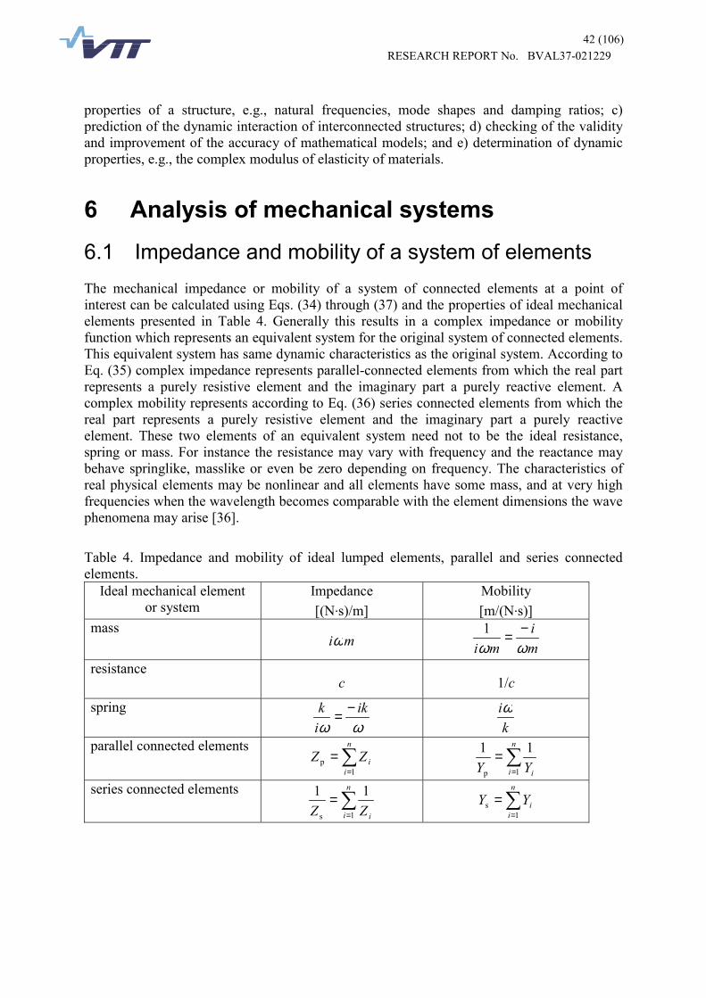
5.2 Applications of mechanical mobility measurements ....................................... 416 Analysis of mechanical systems ................................................................ 42
6.1 Impedance and mobility of a system of elements........................................... 426.2 Kirchhoff´s Laws............................................................................................. 436.3 Superposition theorem ................................................................................... 436.4 Reciprocity theorem ....................................................................................... 436.5 Thévenin´s equivalent circuit .......................................................................... 436.6 Norton´s equivalent circuit.............................................................................. 456.7 Analysis methods ........................................................................................... 466.8 Example of analysis ....................................................................................... 46
7 Impedance and mobility parameters .......................................................... 507.1 Impedance parameters .................................................................................. 507.2 Mobility parameters ........................................................................................ 51
8 Four-pole parameters of mechanical systems .......................................... 538.1 Theory ............................................................................................................ 538.2 Four-pole parameters of a series connected system ..................................... 558.3 Four-pole parameters of a parallel connected system.................................... 568.4 Four-pole parameters of lumped systems ...................................................... 56
8.4.1 Mass...................................................................................................... 568.4.2 Spring .................................................................................................... 578.4.3 Resistance............................................................................................. 578.4.4 Parallel spring and resistance................................................................ 588.4.5 Dynamic absorber ................................................................................. 588.4.6 Dynamic absorber in a mechanical system ........................................... 59
9 Characterization of structure-borne sound source................................... 609.1 Introduction .................................................................................................... 609.2 Complex power transmission ......................................................................... 60
9.2.1 Constant velocity and constant force source ......................................... 629.2.2 Transmission loss of elastic elements ................................................... 629.2.3 Source descriptor and coupling function................................................ 63
9.2.3.1 One-point-connected systems ................................................................................. 639.2.3.2 Multi-point-connected systems ................................................................................ 65
9.2.4 Characteristic power.............................................................................. 6710 Mobility functions and free velocities ........................................................ 69
10.1.1 Machine mobilities ................................................................................. 6910.1.1.1 Mobility in mass controlled region............................................................................ 7010.1.1.2 Mobility in stiffness controlled region ....................................................................... 7110.1.1.3 Mobility in resonance controlled region.................................................................... 71
10.1.2 Floor mobilities ...................................................................................... 7210.1.3 Free velocities of machine..................................................................... 72

5 (106)RESEARCH REPORT No. BVAL37-021229
11 Measurement techniques ............................................................................ 7311.1 Mobility measurement ........................................................................... 73
12 Structure-borne sound power transmission from machines ................... 7412.1 Power calibration of receiving structure................................................. 74
12.1.1 Introduction............................................................................................ 7412.1.2 Power transmission from source machine to receiving structure........... 74
12.1.2.1 Power transmission estimate over contact zone ..................................................... 7512.1.3 Power calibration of receiving structure................................................. 75
12.1.3.1 Calibration of receiving structure ............................................................................. 7512.1.3.2 Reference power estimate ....................................................................................... 7712.1.3.3 Calibration with source machine installed................................................................ 77
12.1.4 Application examples............................................................................. 7912.1.4.1 Box receiver and engine foundation of ship............................................................. 7912.1.4.2 Helicopter fuselage .................................................................................................. 82
12.1.5 Applicability of in-situ estimation method............................................... 8312.2 Surface power or equivalent source power............................................ 83
12.2.1 Excitation and response points.............................................................. 8412.2.2 Machinery mounting conditions ............................................................. 85
13 Power transmission through vibration isolator......................................... 8613.1 Dynamic stiffness matrix and general concepts..................................... 8613.2 Determination of power transmitted via vibration isolator ...................... 90
13.2.1 Direct method ........................................................................................ 9013.2.2 Indirect method...................................................................................... 9013.2.3 Generalization of the indirect method .................................................... 92
14 Research and test facilities of vibration isolators..................................... 93
14.1.1 Research and facilities at KTH, Sweden ............................................... 9314.1.2 Research and facilities at AMRL, Australia............................................ 9614.1.3 Research and facilities at TNO TPD, The Netherlands ......................... 9714.1.4 Research and facilities at HUT and VTT, Finland................................ 100
15 Conclusions................................................................................................ 101
References ............................................................................................................ 102
6 (106)RESEARCH REPORT No. BVAL37-021229
1 IntroductionToday acoustics of vehicles or any kind of machines is important for the community and theindustry. This interest in sound and vibration quality has been seen as numerous internationaland national regulations given for sound and vibration control to reduce the impact on man.
Low noise design ([1], [2], and [3]) and design of quiet structures [4] are getting moreemphasis at the design stage and it has an important impact on the marketability andcompetitiveness of many products. At the design stage it is often asked to predict the resultedsound levels of a machine or component. To do this, one needs to analyze all the excitationsources and their interactions with the structures and transmission paths. For air-borne soundwell-established design and measurement methods are nowadays available. Instead forstructure-borne sound the methods for characterization of machines or components as sourcesof structure-borne sound are still in phase of intensive research and development.
Sound is propagated over long distances in built-up structures mainly as structure-bornesound because of low material damping. Instead air-borne sound has only meaning near thesound source or in spaces contiguous to the source space. Audible sound to a normal humanear covers roughly the frequency range from 20 Hz to 20 kHz [5, p. 25]. Usually at the designstage the frequency range is restricted to the frequencies including the octave bands from31,5 Hz to 8 kHz. This means that in built-up systems composed typically of beams, platesand shells one or two dimensions are small compared with the structural wavelength. Thisrequires very much from the analysis methods and engineers when typically only scarce inputdata is available to meet the requirements specified on a new product.
Analysis methods of structure-borne sound transmission must be able to handle withdifferent parts of the structure and with the whole structure as well. Substructuring techniqueallows the properties of the assembled structure to be calculated using the properties of itsparts. In the modelling using substructuring one important requirement is to be able to utilizealso measured input data because the properties of mechanical parts vary and sometimes theonly way is to use measured input data. The so-called impedance or mobility method allowsboth substructuring and use of measured input data [6]. The roles of experiments withcomputational experimentation are thoroughly discussed by Frank Fahy in [7].
Structural parts may be modelled and analyzed using several methods including theoreticaland experimental modal methods, discrete Finite Element Methods (FEM) or using the meanvalue methods like Statistical Energy Analysis (SEA) [8]. Depending on the modelling workat hand, sometimes even empirical and semiempirical methods have to be used.
Characterization of machines as sources of structure-borne sound is the major problemwhen estimating the structure-borne sound emission [9]. Vibrational power transmission froma machine source to flexible machinery supporting structures has been under intensiveresearch (see e.g., references [10], [11], [12], [13], [14], [15], [16], [17], [18] and [19]). Powertransmission from a source structure to the receiving structure depends on the mobilities ofthe source and the receiving structure, respectively.

7 (106)RESEARCH REPORT No. BVAL37-021229
This literature review is concentrated to the structure-borne sound power and sourcecharacterization of diesel engines in the ship context (see Figure 1) and in an agriculturaltractor (see Figure 2). The mobility technique is discussed as well, because it is well knownthat the transmitted power from source to the receiving structure is dependent on themobilities of the source and the receiver. Also the determination of vibrational powertransmission through vibration isolators is reviewed.
Motor Gear Propeller
Water
Figure 1. In the ship and small graft context interaction phenomena interconnect sources ofsound and vibration with structures and the surrounding air and water.
Figure 2. Diesel engine as a source of structure-borne sound in an agricultural tractor.
2 Definitions2.1 Acoustics and soundAcoustics is the science of sound (see [5]). It includes generation, transmission, and effects ofsound. The term sound means not only the phenomena in air which cause the sensation ofhearing but also those phenomena that are governed by analogous physical principles. Thuswe use the terms infrasound and ultrasound even the frequency is either too low or too high tobe heard by a person with normal hearing. In addition the terms underwater sound, sound insolids, and structure-borne sound are in common usage. The frequency range of audiblesounds is roughly between 20 Hz and 20 000 Hz. Compared to optics sound is a mechanicalwave motion whereas light is an electromagnetic wave motion.

8 (106)RESEARCH REPORT No. BVAL37-021229
2.2 Airborne soundSound that is transmitted from the sound source to its environment through air is calledairborne sound. It propagates as longitudinal compressional waves. The speed of sound in airis about 340 m/s. A wave is a process where a disturbance from equilibrium in a materialmedium is transported through the medium without net transport of mass [20].
2.3 Structure-borne soundMany sounds, which we sense to come from different activities, are either produced orconducted by vibrating solid bodies. These include for instance the sound of many musicalinstruments, engines, machines and the impact sound coming from the adjoining room. Thefield of physics which deals with the generation and propagation of motions and forcesvarying as a function of time in solid bodies and the associated sound radiation is called"structure-borne sound" [23]. Or alternatively structure-borne sound covers all forms ofaudio-frequency vibration of solid structures, because these vibrations are inevitablyaccompanied by the generation of sound in contiguous fluids [20]. In this context sound refersto the frequency range of interest that is the frequency range audible to a normal human earroughly between 20 Hz and 20 kHz. However, the frequency limits are not to be considered asabsolute limits [23]. The phenomena associated with structure-borne sound are complicatedbecause sound is propagated in many waveforms, which couple with each other at structuraljunctions. In addition the speed of wave propagation may depend on frequency, as is the casewith bending (flexural) waves. The range of amplitudes of structure-borne sound varies fromless than 810− mm at high frequencies to several millimeters at low frequencies.
2.4 Sinusoidal disturbanceSmall amplitude perturbations compared to an ambient state are called acoustic disturbances.The ambient state ( 000 , , vρp ) for a fluid is characterized by the values of the pressure 0p ,density 0ρ and fluid velocity 0v which prevail when there is no perturbation. Thus forinstance the acoustic pressure is the perturbation equivalent to the deviation from the staticpressure (total pressure) [5]. The hearing threshold for a person with acute hearingcorresponds to the acoustic pressure of 20 µPa equivalent to 0 dB (re 20 µPa) and the pressure63 Pa equivalent to 130 dB corresponds the threshold of pain. These pressures can becompared with the ambient static air pressure of 0,1 MPa to get an idea of the relativemagnitudes of pressures. Also that is why the decibel scale is used to get numbers to apractical scale between 0 - 130 when expressing the magnitude of usually encounteredacoustic pressures.
A field is a constant frequency if the field variables are varying sinusoidally with time,such that for instance for the acoustic pressure p [5]
[ ]tieptptpp ωφωφω −=′−=−= ˆRe)sin()cos( pkpk , (1)
where the amplitude or peak pressure pkp , the angular frequency ω , the complex pressureamplitude p , and the phase constants φ and φ′ are independent of time t. Re [ ] denotes realpart. The relations in Eq. (1) are equivalent, if [5]

9 (106)RESEARCH REPORT No. BVAL37-021229
2πφφ −=′ , φiepp pkˆ = , (2)
since trigonometry and Euler's formula give the following equations, respectively,
απα cos2
sin =��
���
� + , ααα sincos iei += . (3)
The pressure in Eq. (1) oscillates between positive and negative values and repeats itselfwhen the arguments φω −t or φω ′−t change by π2 when the sine or cosine functionchanges sign. Thus the period, the time per cycle, is ωπ /2 and the number of cycles per unittime, frequency, is
πω2
=f , (4)
and the SI unit of frequency is hertz [Hz], where -1s 1Hz 1 = (or one cycle per second). The SIunit of angular frequency is [rad/s] (radians per second) often written in the form of only [1/s].
A plane travelling wave of constant frequency repeats itself also with distance ofpropagation and the repetition length is called wavelength k/2πλ = , where k is the wavenumber. The relationships between wave number, angular frequency, frequency, speed ofsound propagation c and wave length are obtained from
λππω 22 ===
cf
ck . (5)
The complex number representation introduced in Eq. (1) is frequently used in theoreticalstudies because it enables the expression of the amplitude and phase with only one complexnumber. The time dependence tie ω− is traditional in wave-propagation studies [5]. Somewriters use instead the time dependence tie ω+ .
For sinusoidally varying pressure (see Eq. (1)) the mean squared pressure av2 )( p (many
times denoted as )( 2p where the over-bar means time-averaging) and root-mean-squared(rms) pressure rmsp are defined as [5]
2rms
22av
2 0
0
)(1)()( pdttpT
ppTt
t=== �
+, (6)
where T is either an integral number of half-wave periods or an interminably long time. Withthe aid of Eqs. (1) and (6) one gets relationships [5]
2212
pk212
rms2
av2 ˆ)()( ppppp ==== . (7)

10 (106)RESEARCH REPORT No. BVAL37-021229
The spatial averaging over a surface or a volume is denoted often in the literature by anglebrackets, e.g., 2p .
2.5 Time average of a productIf one considers with same frequency oscillating two signals X and Y denoted by
[ ] [ ]titi eYYeXX ωω −− ==��
Re and Re , (8)
then the time average of their product is obtained from [5]
[ ]∗= YXXY avˆˆRe)( 2
1 , (9)
where ∗Y is the complex conjugate of Y . This can be derived for example as follows: usingthe notation of Eq. (8) for X and Y one obtains
[ ] [ ] av-i
avav )(Re)e(Reˆˆ)ˆRe()ˆ(Re)( βαωφωφ itiYitiXi eYXeeYeeXXY −−− ⋅== ,
where Xt φωα −= and Yt φωβ −= . The trigonometric identity [5]
)cos()cos(coscos 21
21 βαβαβα ++−= (10)
gives
[ ] [ ] av21
21
avav )2cos()cos(ˆˆcoscosˆˆ)( XYXY tYXYXXY φφωφφβα −−+−⋅=⋅=where the second term averages out to zero when the time averaging is performed, and oneobtains the relation presented in Eq. (9)
[ ] [ ]∗−± ==⋅=−⋅= YXYXeYXYXXY XYiXY
ˆˆReˆˆRe)ˆˆRe()cos(ˆˆ)( 21*
21)(
21
21
avφφφφ .
2.6 Time average of powerA time-harmonic force being a real quantity can be considered to be of the form
[ ]tieFtF ω−= ˆRe)( . This force excites the structure at the contact point to vibrate with velocity[ ]tievtv ω−= ˆRe)( . The time average of the power P transmitted to the structure by this
excitation can be evaluated using Eq. (9) as ([23], [26], [31])
[ ] [ ] [ ]��∗−− ===
T titiTvFdteveF
TdttP
TP
0 21
0ReReRe1)(1 �
�
�
� ωω , (11)
where )(tP is the instantaneous power at time t, F�
is the complex amplitude of force, v� isthe complex amplitude of velocity, and fπω 2= is the angular frequency at frequency f.This power is only due to the product of force and velocity not including the contribution ofthe product of moment and angular velocity.
11 (106)RESEARCH REPORT No. BVAL37-021229
3 Mechanical impedance and mobility ofelements
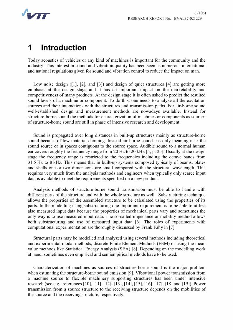
3.1 Force and velocity phasorsThe motion of a linear mechanical system can be expressed with differential equations interms of the driving force and the acceleration, velocity, or displacement of the elements ofthe system. When the driving force is sinusoidal, the steady-state response is also sinusoidal atthe driving frequency with a fixed phase difference to the driving force. Because any time-varying signal may be expressed as a superposition of sinusoids, one may consider onesinusoid at a time and then superpose the results, without loosing generality of analysis [36].
Using the rotating phasor notation the sinusoidally varying force can be presented on thecomplex plane, as shown in Figure 3. The force phasor has a length or magnitude 0F and itrotates counterclockwise with angular velocity ω making the angle tω with the positive realaxis at time t. The real instantaneous force tF ωcos0 is the projection
��
�� �� �� � ��
�� ��� � ��
��
��
�
� � � � � �
����������
Figure 3. A sinusoidal force and velocity in the complex plane.
of the force phasor on the real axis. The force F can be expressed with its real and imaginarycomponents as
tiFtFF ωω sincos 00 += . (12)
It is convenient for the analysis purposes to represent the force in terms of its magnitude 0Fand its phase angle tω as
tieFF ω0= . (13)
A sinusoidally varying velocity can also be represented as a phasor (see Figure 3). If thevelocity phasor, magnitude 0v , is rotating at the same angular velocity ω as the force phasor,magnitude 0F , the velocity v can be represented as
( ) ( )[ ] ( )φωφωφω +=+++= tievtitvv 00 sincos , (14)

12 (106)RESEARCH REPORT No. BVAL37-021229
where φ is the phase angle between the force F and velocity v, and the velocity is leading theforce with angle φ. If the phase reference is force F instead of the positive real axis, then thevelocity may be given as
φievv 0= . (15)
The displacement x of a sinusoidal vibration is obtained by integrating the velocity expressedas tievv ω
0= , and noticing that �= vdtx as
ωivx = . (16)
The acceleration a of a sinusoidal vibration is obtained from velocity using the relationdtdvxa == �� as
vixa ω== �� . (17)
3.2 Mechanical impedance of lumped elements
3.2.1 Mechanical impedance of resistance
Real physical systems can be modelled using idealized mechanical system elements withlumped constants: resistance, spring, and mass [36]. A mechanical resistance is defined as adevice in which the relative velocity between its end points is proportional to the force appliedto its end points (Figure 4).
���
� ��
�� ��
�
Figure 4. Ideal mechanical resistance element [36].
In an ideal resistance element the force resisting the extension or compression of theelement is viscous friction force. In (Figure 4) the relative velocity of point A relative to pointB is
( )cF
vvv a21 =−= , (18)
where the proportionality constant c is mechanical resistance (or damping constant), and aF isthe viscous friction force acting at point A. If there is a relative velocity at point A as a result

13 (106)RESEARCH REPORT No. BVAL37-021229
of force aF acting on it, there must be a reaction force at point B of equal strength. Thevelocities 1v and 2v are measured relative to a common stationary reference point G.
When the sinusoidal force tieF ω0 (Eq. (13)) is acting on the ideal resistance element at the
point A and the point B is attached to a fixed point, then the velocity of point A is obtainedfrom Eq. (18) as
titi
evceF
v ωω
00
1 == . (19)
From Eq. (19) it is seen that the force and the resulted velocity phasors are rotating at thesame angular velocity ω and that they are in the same phase (see Figure 5).
��
�
�� �� �
��
� � � � � �
����������
Figure 5. Force (magnitude 0F ) acting upon an ideal resistance results in a velocity(magnitude 0v ) in the same phase, adapted from [36].
Using Eq. (13) and (19) one gets for the mechanical impedance of a resistance element as
ce
cF
eFvFZ
ti
ti
===ω
ω
0
0c . (20)
From Eq. (20) it is seen that the impedance of a resistance is equal to its damping constant c.
3.2.2 Mechanical impedance of spring
A linear spring is defined as a device for which the relative displacement between its endpoints is proportional to the force acting on the spring in its main direction. The displacementof the end points of a spring is mathematically represented as (Figure 6)
kF
xxx a21 =−=δ , (21)
where k is the spring stiffness and 1x and 2x are the displacements of the end points A and Brelative to the stationary point G.

14 (106)RESEARCH REPORT No. BVAL37-021229
�
�
��
�
��
��
��
Figure 6. An ideal spring. The force aF is acting on the end point A causing the reactionforce ab FF = at point B. The spring stiffness is k, 1v and 2v are the velocities of the endpoints relative to a stationary point G, adapted from [36].
If the point B is fixed, and one applies the force of Eq. (13), then the displacement of pointB is obtained from Eq. (21) as
titi
exkeFx ω
ω
00
1 == . (22)
It is seen from Eq. (22) that the displacement varies sinusoidally at the same angularfrequency as the applied force and that it is in the same phase with the force. The velocity 1vof the end point A is obtained by differentiating the displacement with respect to time t, so
titi
eivkeFi
xv ωωω
00
11 === � . (23)
From Eq. (13) and (23) one obtains the mechanical impedance of an ideal spring as
ωωω ω
ω ikik
keFieF
vFZ ti
ti
k−====
0
0 . (24)
It is seen from Eq. (24) that the impedance of an ideal spring is imaginary and depends on thespring stiffness k and the angular frequency ω. The velocity in Eq. (23) may be written in theform of Eq. (12) as
)2(0
01 )cossin( πωωωωωω +=+−= tieF
ktit
kFv . (25)
From Eq. (25) it is seen that the velocity phasor of an ideal spring leads the force phasor bythe angle °= 902π (see Figure 7). The same thing is indicated by the imaginary unit i in theEq. (23), because iiiei i =+=+== 0sincos 22
2 πππ .
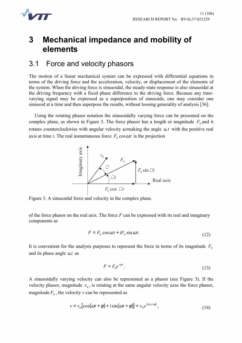
15 (106)RESEARCH REPORT No. BVAL37-021229
�
�� ��
��
��
� � � � � �
����������
�� �
��
Figure 7. Force (magnitude 0F ) and velocity (magnitude 0v ) phasors at the end point of anideal spring, adapted from [36].
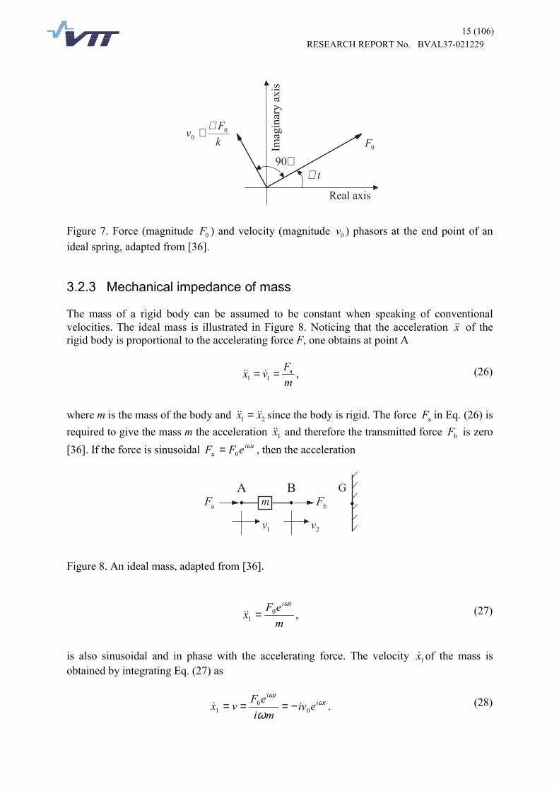
3.2.3 Mechanical impedance of mass
The mass of a rigid body can be assumed to be constant when speaking of conventionalvelocities. The ideal mass is illustrated in Figure 8. Noticing that the acceleration x�� of therigid body is proportional to the accelerating force F, one obtains at point A
mFvx a
11 == ��� , (26)
where m is the mass of the body and 21 xx ���� = since the body is rigid. The force aF in Eq. (26) isrequired to give the mass m the acceleration 1x�� and therefore the transmitted force bF is zero[36]. If the force is sinusoidal tieFF ω
0a = , then the acceleration
��
� ��
�� ��
�
�
Figure 8. An ideal mass, adapted from [36].
meF
xtiω
01 =�� , (27)
is also sinusoidal and in phase with the accelerating force. The velocity 1x� of the mass isobtained by integrating Eq. (27) as
titi
eivmi
eFvx ω
ω
ω 00
1 −===� . (28)

16 (106)RESEARCH REPORT No. BVAL37-021229
Dividing the force tieFF ω0a = by the velocity given in Eq. (28) one obtains the mechanical
impedance of the mass as
mimieF
eFvFZ ti
ti
m ωωω
ω
===/0
0 . (29)
From the Eq. (29) one sees that the mechanical impedance of the mass is imaginary anddepends on the magnitude of mass and on the angular frequency. The velocity in the Eq. (28)can be written in the form
)2(00 )cos(sin πω
ωωω
ω−=−= tie
mF
titm
Fv . (30)
From Eq. (30) it is seen that the phasor of the velocity is °= 902π behind the force phasor(see Figure 9), this is indicated also by -i in Eq. (28).
�
��
��
� �
��
� � � � � �
����������
�� �
��
Figure 9. Force and velocity phasor of ideal mass in the complex plane, adapted from [36].
The magnitude of the mechanical impedance of ideal mass, resistance and spring as a functionof frequency is presented schematically in Figure 10.
0
2
4
6
8
10
12
14
16
18
0 1000 2000 3000 4000 5000 6000 7000 8000 9000 10000
Frequency [Hz]
Impe
danc
e [N
s/m
]
ωkZk = mZm ω=
cZc =
Figure 10. The magnitude of the mechanical impedance of ideal resistance, spring and mass,adapted from [36].

17 (106)RESEARCH REPORT No. BVAL37-021229
3.3 Mechanical mobility of lumped elementsReal structures or physical systems can be modelled using idealized mechanical elements withlumped constants. Such elements are mechanical resistance (or damping), spring, and mass.For these elements the mobilities are [36]:
resistance:c
Yc1= ,
(31)
where c is mechanical resistance with SI unit [ ]s)/m(N ⋅ ;
spring:k
iYkω= , (32)
where k is spring stiffness with SI unit [N/m]; and
mass:mi
miYm ωω
−== 1 , (33)
where m is element mass with SI unit [kg]. The mobility magnitude as a function of frequencyof these idealized mechanical elements is presented in Figure 11.
0
2
4
6
8
10
12
14
16
18
0 1000 2000 3000 4000 5000 6000 7000 8000 9000 10000
Frequency [Hz]
Mob
ility
[m/(N
s)] m
Ym ω1=
kYk
ω=
cYc
1=
Figure 11. The mobility magnitudes of an ideal mechanical resistance cY , spring kY and
mass mY as a function of frequency.
3.4 Impedance and mobility of connected elements
3.4.1 Impedance and mobility of parallel connected elements
The properties of mechanical systems can be analyzed using mechanical impedance ormobility concepts. In the analysis impedance and mobility are determined at the points offorce excitation or paths for transmitting forces, or at points of common velocities [36]. In

18 (106)RESEARCH REPORT No. BVAL37-021229
Figure 12 the exciting force F causes the common velocity at the connection point A, which iscommon for the parallel connected spring and resistance.
�
�
�
�
��
Figure 12. Schematic presentation of a mechanical system consisting of a spring (springstiffness k) and a mechanical resistance (resistance c) connected parallel at points A and B.The exciting force F gives a common velocity v for both elements at point A referred to thestiff point B.
The force required to give the resistance the velocity v is obtained from Eqs. (39) and (31)
cv
YvFc
c 1== .
The force required to give this same velocity for the spring is obtained from Eqs. (39) and(32)
kiv
YvFk
k ω== .
The total force F is the sum of parallel forces
p
111
Yv
kicvFFF kc =�
�
���
� +=+=ω
.
From this it is seen that the inverse of the total mobility pY of the parallel-connected elementsis
�=
=n
i iYY 1p
11 , (34)
where n is the number of parallel-connected elements. The total impedance pZ of parallel-connected elements can be obtained from [36]
�=
=n
iiZZ
1p , (35)
where n is the number of parallel-connected elements with mechanical impedances iZ .

19 (106)RESEARCH REPORT No. BVAL37-021229
3.4.2 Impedance and mobility of series-connected elements
Another basic way of connecting elements is series connection, which is presented in Figure13.
�� �
�� ��
� ��
�� ��
Figure 13. A system consisting of two series-connected mechanical elements with mobilities1Y and 2Y . The exciting force F gives relative velocities av and bv between the end
connections of each element. The velocities of the connection points 1 and 2 relative to thestationary reference are 1v and 2v .
The velocities of the connection points 1 and 2 are:b2 vv = and ab2121 )( vvvvvv +=−+= .
The total mobility at point number 1 is FvY /1= , and the same force F is acting on bothelements. The relative velocities expressed with mobilities are:
1a FYv = and 2b FYv = .So the total mobility is
2121ba1 YY
FFYFY
Fvv
FvY +=+=+== .
The total mobility sY of n series connected elements is thus
�=
=n
iiYY
1s , (36)
where iY is the mobility of element i.
The total impedance sZ of ideal series connected elements is obtained from
�=
=n
i iZZ 1s
11 , (37)
where n is the number of series-connected elements with mechanical impedances iZ .
20 (106)RESEARCH REPORT No. BVAL37-021229
4 Impedance and mobility concepts4.1 Generalized mechanical mobility
Consider a linear and time invariant system, which is excited by a force field )exp( tif ω⋅�
expressed as complex force amplitude f�
times a harmonically varying function of time)exp( tiω . Owing to the system linearity the corresponding velocity field is also harmonic,
)exp( tiv ω⋅� , and the ratio fv�
� / is independent of the amplitude of the exciting force [6].When the excitation is harmonic at angular frequency ω, the generalized mechanical mobilitycan be defined as the ratio between the complex amplitudes of the velocity field and the forcefield as [6]
)()()(
ωωω
fvy �
�
= .(38)
4.2 Mechanical mobilityISO 7626-1 [21] defines mechanical mobility ijY as: "The frequency-response functionformed by the ratio of the velocity-response phasor at point i to the excitation force phasor atpoint j, with all other measurement points on the structure allowed to respond freely withoutany constraints other than those constraints which represent the normal support of thestructure in its intended application." The definition is given mathematically in Eq. (39)
jiij FvY = , (39)
where iv is the velocity-response phasor at point i and jF the force phasor at point j.
The velocity response can be either translational or rotational, and the excitation can beeither a rectilinear force or a moment. Frequency response function is defined as thefrequency dependent ratio of the motion-response phasor to the phasor of the excitation force[21].
Mechanical mobility is sometimes called mechanical admittance. Likewise the complexmobility Y can be written as
iBGY += , (40)
where the real part G is called the conductance and the imaginary part B the susceptance. TheSI unit of mechanical mobility is [ ]s)m/(N ⋅ .
21 (106)RESEARCH REPORT No. BVAL37-021229
4.3 Driving-point and transfer mobilityDirect (mechanical) mobility or driving-point (mechanical) mobility iiY is the complex ratioof velocity and force taken at the same point in a mechanical system during simple harmonicmotion [22]. Here point means both a location and a direction. Sometimes the term co-ordinate is used instead of point. Transfer mechanical mobility ijY is the complex ratio of thevelocity iv measured at the point i in the mechanical system to the force excitation jF at thepoint j in the same system during simple harmonic motion [22].
4.4 ImpedanceImpedance is defined as the complex ratio of a harmonic excitation of a linear system to itsresponse during simple harmonic vibration. Both the excitation and the response are complexand their magnitudes increase linearly with time at the same rate [22].
4.5 Mechanical impedanceThe mechanical impedance is defined in a mechanical system as the complex ratio of force tovelocity as [23], [24]
vFZˆˆ
= , (41)
where F is the phasor of the exciting force, and v is the phasor of the velocity as a responseat the excitation region. The mechanical impedance is generally a complex function offrequency, because the force and resulting velocity vary with frequency. This generaldefinition is not unique, because the excitation region can be a finite area, and the velocity canvary within this area.
4.6 Moment impedanceIn practical situations the force impedance does not cover all the possibilities. Especially thisis true in the case of flexural vibrations when moments and angular velocities are of equalimportance as forces and translational velocities. The moment impedance W is defined withthe exciting moment M and the resulting angular velocity w as [23]
wMW = . (42)
The force and moment impedances are not enough to describe completely the response fora point excitation; in general a coupling term is needed [23]. So one must consider carefully ifthere is only a force or moment excitation and if any coupling terms are needed.

22 (106)RESEARCH REPORT No. BVAL37-021229
4.7 Driving-point and transfer impedanceDriving-point impedance of a linear mechanical system undergoing sinusoidal vibration isdefined as the complex ratio of the exciting force to the velocity response when both are takenat the same point [22]. Here point means both a location and a direction.
When measuring the point impedance of beam or plate structures, the diameter of thecontact area should be less than one-tenth of a flexural wavelength, and not much less than thethickness of the structure under measurement [23].
Transfer impedance of a linear mechanical system undergoing sinusoidal vibration isdefined as the complex ratio of the exciting force to the velocity response at another point[22]. Here point means both a location and a direction.
4.7.1 Driving-point impedances of infinite plates and beams
In Table 1 is given some impedance formulas of practical interest in noise control work. Inmany practical problems these impedance formulas can be applied for finite built-upstructures when the frequency is high enough as often is when consideration is given tostructure-borne sound.

23 (106)RESEARCH REPORT No. BVAL37-021229
Table 1. Driving-point impedances of infinite beams and plates [23].
4.8 Driving-point mobilityMechanical driving-point mobility is defined as the frequency response function formed bythe ratio of the velocity response phasor at point i to the excitation force phasor at the samepoint i. The velocity response can be either translational (velocity v) or rotational (angularvelocity θω �= , where θ is angular displacement), and the excitation force can be either arectilinear force F or torque T.

24 (106)RESEARCH REPORT No. BVAL37-021229
4.8.1 Driving-point mobility of infinite plates and beams
The driving-point mobilities given in Table 2 apply to infinite structures in which noresonances can occur. In real finite structures there are always reflections from discontinuitiese.g. from junctions and these usually give a resonant response. The damping in the structurecontrols the magnitude of the vibration amplitudes in the resonance. Usually the largestamplitude will occur at the first resonance frequency. So the largest error in the response willoccur at the resonance frequency if the finite structure is replaced by an equivalent infinitestructure. The driving-point mobility of a finite structure (for e-iωt notation) can be written as[27]
[ ]� −−
−=N n
n
ii
Fv
22
2
)1( ωηωψω , (43)
where nω is the real resonance angular frequency, η the hysteretic loss factor, n the modenumber, and nψ is the amplitude of the mode shape. If the damping is small then the effect ofthe off-resonance terms is small on the amplitude. For a finite structure an approximatedriving-point mobility can be written as
[ ]ηω
ψn
n
Fv 2
= , (44)
if the spacing between resonances is large [27].
If the largest peak mobility values are used when a finite structure is modelled usingmobilities of an infinite structure, then the worst case and the largest errors are obtained [27].The ratio of the point mobility of a finite structure to the point mobility of an infinite structureis also represented in Table 2. From this table it is seen that in practical cases a goodapproximate mobility is obtained if the properties of an infinite structure is used whenestimating the properties of a finite structure.

25 (106)RESEARCH REPORT No. BVAL37-021229
Tabl
e 2.
Pro
perti
es o
f inf
inite
syst
em (n
otes
: *, t
orqu
e ap
plie
d ab
out a
xis p
aral
lel t
o l 2;
tim
e de
pend
ence
of f
orm
eiω
t
assu
med
) [27
].

26 (106)RESEARCH REPORT No. BVAL37-021229
Tabl
e 2.
Con
tinue
d

27 (106)RESEARCH REPORT No. BVAL37-021229
Table 2. Continued. List of symbols [27].
4.9 Mechanical free impedance and compleximpedance
The mechanical free impedance ijZ is defined as the ratio of the excitation force phasor jF atpoint j to the resulting velocity response-phasor iv at point i, with all other connection points(Here point means both a location and a direction.) of the system having zero restrainingforces
iji
jij Yv
FZ 1== . (45)
Free impedance is the arithmetic reciprocal of a single element of the mobility matrix.
ISO 7626-1 [21] gives two important notes when utilizing measured or analyticalimpedance data: "1) Historically, no distinction has often been made between blockedimpedance and free impedance. Caution should, therefore, be exercised in interpretingpublished data. 2) While experimentally determined free impedances could be assembled intoa matrix, this matrix would be quite different from the blocked impedance matrix resultingfrom mathematical modelling of the structure and, therefore, would not conform to therequirements discussed in annex A for using mechanical impedance in an overall theoreticalanalysis system."
The complex impedance Z can be written as
iXRZ += , (46)
where the real part R is called the resistance and the imaginary part X the reactance. The SIunit of the mechanical impedance is [ ]s)/m(N ⋅ .

28 (106)RESEARCH REPORT No. BVAL37-021229
4.10 Blocked mechanical impedanceISO 7626-1 [21] defines blocked impedance ijZ as follows: "The frequency-responsefunction formed by the ratio of the phasor of the blocking or driving-point force response atpoint i to the phasor of the applied excitation velocity at point j, with all other measurementpoints on the structure "blocked" (i.e. constrained to have zero velocity). All forces andmoments required to constrain fully all points of interest on the structure shall be measured inorder to obtain a valid blocked impedance matrix. Blocked impedance measurements (seeCansdale, R. & al. A technique for measuring impedances of a spinning model rotor.Technical report TR 71092, Royal Aircraft Establishment, Farnborough, United Kingdom,May 1971) are, therefore, seldom made and are not dealt with in the various parts of ISO7626. Notes: 1) Any changes in the number of measurement points or their location willchange the blocked impedances at all measurement points. 2) The primary usefulness ofblocked impedance is in the mathematical modelling of a structure using lumped mass,stiffness and damping elements or finite element techniques. When combining or comparingsuch mathematical models with experimental mobility data, it is necessary to convert theanalytical blocked impedance matrix into a mobility matrix, or vice versa, as discussed inannex A."
4.11 Frequency response functions related to mobilityOther frequency-response functions, structural response ratios, which are used instead ofmobility, are shown in Table 3.
Table 3. Equivalent definitions to be used for various kinds of measured frequency responsefunctions related to mechanical mobility [21].
Motion expressedas velocity
Motion expressedas acceleration
Motion expressedas displacement
Term Mobility Accelerance Dynamic complianceSymbol
jiij FvY /= ji Fa / ji Fx /Unit s)m/(N ⋅ -12 kg)sm/(N =⋅ m/NBoundary conditions jkFk ≠= ; 0 jkFk ≠= ; 0 jkFk ≠= ; 0Comment Boundary conditions are easy to achieve experimentallyTerm Blocked impedance Blocked effective mass Dynamic stiffnessSymbol
jiij vFZ /= ji aF / ji xF /Unit s)/m(N ⋅ kgm/)s(N 2 =⋅ N/mBoundary conditions jkvk ≠= ; 0 jkak ≠= ; 0 jkxk ≠= ; 0Comment Boundary conditions are very difficult or impossible to achieve
experimentallyTerm Free impedance Effective mass (free
effective mass)Free dynamic stiffness
Symbolijij YvF /1/ = ij aF / ij xF /
Unit s)/m(N ⋅ kgm/)s(N 2 =⋅ N/mBoundary conditions jkFk ≠= ; 0 jkFk ≠= ; 0 jkFk ≠= ; 0Comment Boundary conditions are easy to achieve, but results shall be used with
great caution in system modelling

29 (106)RESEARCH REPORT No. BVAL37-021229
4.12 Boundary conditions of experimentationIn experimental determination of mechanical mobility, a dynamic exciting force is applied tothe structure at one point at a time. Thus the force boundary conditions are [21]
jkFk ≠= ; 0 , (47)
where j is the point of excitation and k denotes all other points of interest. When the sameforce boundary conditions are valid, measurement of the velocity response at point i and theexciting force at j yields the ijth element of the mobility matrix [21]:
jkFjiji kFvY ≠== ; 0 )/( . (48)
These force boundary conditions can easily be achieved in practise.
Instead the elements of the impedance matrix Z are [21]:
jiji vFZ /= , (49)
where the boundary conditions
jkvk ≠= ; 0 (50)
are very difficult or impossible to fulfil in practice. Eqs. (49) and (50) describemathematically the definition of blocked impedance. These boundary conditions imply that itis not generally possible to determine experimentally the impedance matrix. The differencebetween force and velocity boundary conditions (Eqs. (47) and (50)) must be kept in mindwhen using mobility and impedance data.
4.13 Mechanical mobility and impedance matrices
4.13.1 Definitions
It is assumed that linear, elastic structures are being considered, so that superposition andnormal calculation rules are valid. The set of mobility elements ijy is defined as follow [30]:
�=j
jjii fyv . (51)
The set of impedance elements is defined as follow [30]:
�=j
jjii vzf . (52)

30 (106)RESEARCH REPORT No. BVAL37-021229
4.13.2 Mechanical mobility matrix
Mechanical mobility is a tensor (or tensor component) which describes the effects upon theresultant velocity of the application of a force or forces on a structure [30]. It can be presentedin the frequency domain by a matrix Eq. [30]:
( )ωωω FYV )()( = , (53)
where fπω 2= is the angular frequency, f is frequency, )(ωF is the column vector ofexciting forces at various points, )(ωV is the column vector of velocity responses at thepoints of interest, and )(ωY is symmetric tensor of mobilities ijy . This matrix Eq. (53) in theexpanded form looks like
etc. , , , ,
3432421414
3332321313
3232221212
3132121111
�
�
�
�
+++=+++=+++=+++=
fyfyfyvfyfyfyvfyfyfyvfyfyfyv (54)
The term jji fy defines a velocity at point i caused by a force acting at a point j. If thisvelocity is noted by jiv , then [30]
�=j
jii vv . (55)
It is seen from this equation that the mobility is a concept that sums velocity response [30].
The elements of the matrix Y can be measured by applying the forces one at a time to eachpoint of interest allowing the structure to response as it chooses, and the individual elementsare obtained as the complex ratio of the particular velocity response to the single excitingforce. If for example only the force 2f is applied, then Eq. (54) would reduce to the set [30]
,23232
,22222
,21212
fyvfyvfyv
=== (56)
and so on, since 2 ,0 ≠= kfk . Then the element 12y is the obtained as the complex ratio
21212 / fvy = , etc. (57)
The reciprocity theorems of vibrations hold, and thus ijji yy = [30].
31 (106)RESEARCH REPORT No. BVAL37-021229
4.13.3 Impedance matrix
Impedance is a tensor (or tensor component) which describes the effects upon the resultantforce (or several forces) of the application of a velocity or velocities on the structure. [30].This can be represented by the matrix equation
)()()( ωωω VZF = , (58)
where fπω 2= is the angular frequency, f is frequency, )(ωF is the column vector ofresultant forces if , )(ωV is the column vector of applied velocities jv , and )(ωZ issymmetric tensor of impedances ijz . This matrix equation can be expanded as follow [30]
etc. , , , ,
3432421414
3332321313
3232221212
3132121111
�
�
�
�
+++=+++=+++=+++=
vzvzvzfvzvzvzfvzvzvzfvzvzvzf
(59)
The term jji vz defines a force at the point i caused by an applied velocity at the point j. If
this force is called jif , then
�=j
jii ff . (60)
From Eq. (60) it is seen, that impedance is a concept that sums force response [30].When determining the elements of impedance matrix Z the velocities are applied one at atime to each point of interest, the structure is not allowed to response freely, instead it isconstrained to have zero velocity at the points where other velocities will be applied, and theindividual elements are obtained as the complex ratio of the particular force response to thesingle exiting velocity [30]. Consider an example were only the velocity 2v is applied on thestructure at the point 2 then the Eq. (59) will reduce to the set
,,,
23232
22222
21212
vzfvzfvzf
=== (61)
and so on, since 2 ,0 ≠= kvk . In this case 2)( 2 ≠jf j is the blocking (constraining) force atthe point j, when the structure is excited by a velocity at the point 2, which is necessary toconstrain the velocity at the point j to zero, and 22f is the force which results from theexcitation motion at the point 2 [30]. The element of the impedance matrix is obtained from
222 / vfz jj = . (62)
According to reciprocity ijji zz = [30]. From Eqs. (53) and (58) it is easily seen that1−= YZ . According to matrix calculation the individual elements of impedance matrix are

32 (106)RESEARCH REPORT No. BVAL37-021229
not the arithmetic reciprocals of the elements of the mobility matrix, and vice versa, that is1−≠ kiki yz except in the trivial case of only one point [30].
Notice that the point means the location and the corresponding direction. If in a system thenumber of points is N, then the order of vectors is N and the order of matrices is N x N. Theconcept of immittance (impedance or admittance) and transmission matrices in the context ofthe vibration of mechanical systems is discussed in [33]. The mobilities on the contrary to theimpedances of a given structure do not interdepend upon both the location and number ofpoints of interest [30]. Mobilities describe invariant characteristics of the whole structure;instead impedances describe only substructures. During the mobility measurements theobservations made anywhere on the system do not affect each other. Thus the mobilityelement jiy remains the same although measurements are made at other points. Instead theimpedance elements depend upon the number of observation points and the set of blockingforces used. So the impedance elements cannot be considered as invariant characteristics ofthe structure [30].
In some applications a complete mobility matrix has to be measured for the description ofthe dynamic characteristics of a structure. So translational forces and motions along threemutually perpendicular axes as well as moments and rotational motions may be required to bemeasured depending on the applications. These measurements result in a 6 x 6 mobilitymatrix for each measurement location. For N measurement locations this means a full 6N x6N mobility matrix.
However, in practice only seldom the full mobility matrix needs to be measured. Usually itsuffices to measure only the driving-point mobility in the excitation location and a fewtransfer mobilities in locations of interest on the structure. Sometimes the dynamics of thesystem needs to be determined only in one co-ordinate direction, e.g., in vertical direction.Also in many practical engineering applications the influence of rotational motions andmoments is negligible.
5 Effective mobility5.1 DefinitionsThe elements of the mobility matrix are independent of the number of contact points. This isadvantageous in practical analysis of the dynamical behaviour of structures. The mobility canbe defined generally as [30], [37]
6 , ,2 ,1, ; , ,2 ,1, , �� === jiNmkFv
Y mj
kimk
ji ,(63)
where mjF is the complex force applied in the direction j on an area m which is assumed to be
small compared with the wavelength, and kiv is the complex spatially averaged velocity of
another point k in the direction i due to that force. If the system considered consists of passiveand linear elements, the reciprocity principle is valid and the mobility matrix is symmetric. Inthis case the indices of the elements can be transposed, if sub- and superscripts are transposed
33 (106)RESEARCH REPORT No. BVAL37-021229
simultaneously [37]. If the subscripts are omitted, the general definition of the mobility foreach direction is [37]
m
kmk
FvY = ,
(64)
where, for mk = , the mobility is called the point mobility of point k and for mk ≠ , themobility is called the transfer mobility from point k to point m.
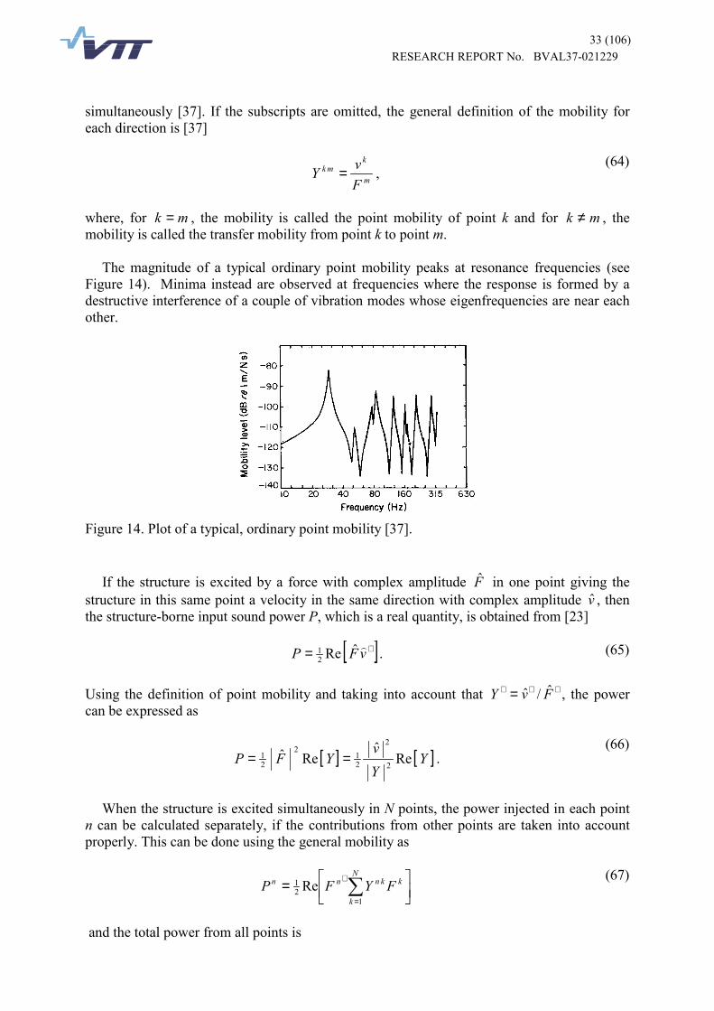
The magnitude of a typical ordinary point mobility peaks at resonance frequencies (seeFigure 14). Minima instead are observed at frequencies where the response is formed by adestructive interference of a couple of vibration modes whose eigenfrequencies are near eachother.
Figure 14. Plot of a typical, ordinary point mobility [37].
If the structure is excited by a force with complex amplitude F in one point giving thestructure in this same point a velocity in the same direction with complex amplitude v , thenthe structure-borne input sound power P, which is a real quantity, is obtained from [23]
[ ]∗= vFP �ˆRe21 . (65)
Using the definition of point mobility and taking into account that ∗∗∗ = FvY ˆ/ˆ , the powercan be expressed as
[ ] [ ]YYv
YFP Reˆ
Reˆ2
2
21
2
21 == .
(66)
When the structure is excited simultaneously in N points, the power injected in each pointn can be calculated separately, if the contributions from other points are taken into accountproperly. This can be done using the general mobility as
��
���
�= �=
∗ N
k
kknnn FYFP1
21 Re
(67)
and the total power from all points is

34 (106)RESEARCH REPORT No. BVAL37-021229
� �= =
∗
��
���
�=N
n
N
k
kknnn FYFP1 1
21 Re .
(68)
5.1.1 Effective point mobility
Let us consider a system with N contact points between the source of structure-borne soundand the receiving structure sketched in Figure 15. Then the transmitted power into the nthcontact point can be calculated from [37]
Figure 15. An example of a multi-point coupled structure-borne sound source and receivingstructure [37].
[ ])()(Re)( 21 ωωω ∗= nnn vFP , (69)
where nF is the complex force and ∗nv is the complex conjugate of the velocity at the samecontact point n.
Considering at the kth contact point the velocity response, which is caused by the forcesacting at all N contact points, the actual velocity kv is obtained using the transfer mobilities
knY from point n to k as
NkNkkkkkk FYFYFYFYv +++++= ��
2211 (70)
the effective point mobility can be defined as [37], [40]
ni
ni
ni
N
k j
kj
nkij
nnii FvFFYY =��
�
����
�= ��
= =
Σ
1
6
1
,(71)
where the superscript Σ means that contributions from all contact points are within thesummation. Remember that the mobility is a concept, which sums (see Eq. (55)) velocityresponse [30]. In the Eq. (71) nkY is the general mobility element when kF is the complexforce acting at point k and velocity is measured at point n. So the effective mobility gives theratio of the total velocity due to all applied forces to the force acting at the same point n.
The power transmitted through the nth connection point is [37]

35 (106)RESEARCH REPORT No. BVAL37-021229
[ ]Σ= nnnn YFP Re221 . (72)
The effective impedance is defined analogously as [37]
nnnN
k
kknnn vFvvZZ =��
���
�= �=
Σ
1
(73)
and using the effective impedance the power is obtained from [37]
[ ]Σ= nnnn ZvP Re221 . (74)
It should be noted that for effective mobility and impedance matrix elements [37]
ΣΣ = nnnn ZY 1 , (75)
whereas for ordinary mobility and impedance matrix elements this relationship does not hold.The negative real part of the effective mobility means that the energy is flowing from thereceiver to the source at that contact point [37]. It can be shown [39] that the real part of theeffective mobility can be calculated from
[ ] [ ] [ ]nnN
nkk
knjknnnnn YeYYYF
ReReReRe1
≈��
�
�
��
�
�+= �
≠=
Σ ϕ ,(76)
which means that the real part of the ordinary mobility can be used. So the structure-bornesound power through the nth contact point is obtained from [37]
[ ] [ ] 22
21
2
21 ReRe Σ=≈ nnnnnnnnn YYvYFP . (77)
The magnitude of the effective mobility ΣnnY can be estimated in two important cases as[37](a) When the magnitudes nkY are approximately alike and the phase angles of nkY arerandomly distributed and furthermore
knYY nnnk ≠≈ allfor , (78)
thennnnn YNY ⋅≈Σ . (79)
(b) When the following inequality holds
knYY nnnk ≠<< allfor , (80)
then the magnitude is obtained from
nnnn YY ≈Σ . (81)

36 (106)RESEARCH REPORT No. BVAL37-021229
5.1.2 Effective total mobility
The power transmitted through all the contact points can be treated formally like in a singlecontact point case. In doing so one needs the effective force defined as [37]
2~vSF EFF = , (82)
where S is the total, transmitted, complex power and 2~v is the spatially averaged meansquare velocity. Analogously to the one contact point case the effective total mobility can bedefined as [37]
SvFvY EFFEFF 22 ~~ == . (83)
If the source and receiver are connected by N similar vibration isolators and the vibrationsare approximately uncoupled between different directions of motion, then the effectivemobility of the receiver can be obtained from [37]
( )2R
122
R
S21
2R
EFFR
~~ kN
k
kkk
kkk vZ
vv
ZvY �=
��
���
����
�
� += ,(84)
where 2R
~v is the average mean square velocity of the receiver, kkZ 21 is the transfer impedance
of one single isolator, kkZ 22 is the input impedance of one isolator seen from the receiver side,kvS and kvR are the complex vibration velocities of the source and receiving structure at the
contact point k, respectively. If the overall effective mobility is developed for the source then22Z is replaced by 11Z for the isolators and 2112 ZZ = due to reciprocity.
Using the effective total mobility the power transmitted to the receiver is obtained from[37]
[ ]{ } 2EFFR
2R
EFFRR
~Re YvYP = . (85)
If the input impedance kkZ 22 is small compared to the other term )/( RS21kkkk vvZ in Eq. (84), the
total power can be approximated by [37]
[ ] 2R
1RS21R )~(/Re k
N
k
kkkk vvvZP �=
≈ .(86)
This approximation is valid when the transfer impedance of the isolator is much smaller thanthe effective point impedance of the receiving structure [37]. A similar result for thetransmitted power is obtained using the effective point impedance, which is obtained from[37]
kkkkkk vvZZ RS21R /≈Σ . (87)
Notice that the effective mobilities are not invariant quantities of the structure. Theeffective point mobility of any point depends on what other points are considered in theanalysis and on the force distribution in that particular case [37].

37 (106)RESEARCH REPORT No. BVAL37-021229
5.1.3 Measurement of effective mobility
Petersson and Plunt [37], [38] examined theoretically and in the laboratory both the effectivepoint mobility and effective overall mobility. The determination of the effective pointmobility was made attaching an accelerometer at one position and exciting the structure witha hammer stroke at this point and the other points sequentially. The force in the stroke area ofthe hammer was measured using a force transducer. At least ten samples of each transferfunction were averaged. This method was applied when the point and transfer mobilities weremeasured. Thereafter the effective point mobility was calculated from Eq. (71) assuming thatthe forces had equal magnitude at each point. During the measurements the structure wasloaded neither by the equipment nor by the experimenter.
The measurement arrangement used during the determination of the effective mobility issketched in Figure 16. In these test a number of vibration isolators was thoroughly tested andmatched with respect their impedance characteristics. The cylindrical
Figure 16. Principal sketch showing the experimental arrangements for the investigations ofthe effective overall mobility [37].
isolators were glued to the measuring object and screwed to the specially designed I-beamabove them. The beam was excited using a vibrator via a steel rod that was attached nearly atthe end of the beam. The velocities and their phase were measured above and below of eachisolator representing a contact point. The overall effective mobility was calculated using Eq.(84). In this equation the impedance characteristics of the isolators are needed in addition tothe measured velocities and their phase angle information.
Petersson and Plunt used a stiffened steel deck mock-up (see Figure 17) and a homogenousconcrete plate as test objects.
Figure 17. Sketch of the stiffened steel deck showing the dimensions (mm), the frame spacingand the measurement positions, [37].
38 (106)RESEARCH REPORT No. BVAL37-021229
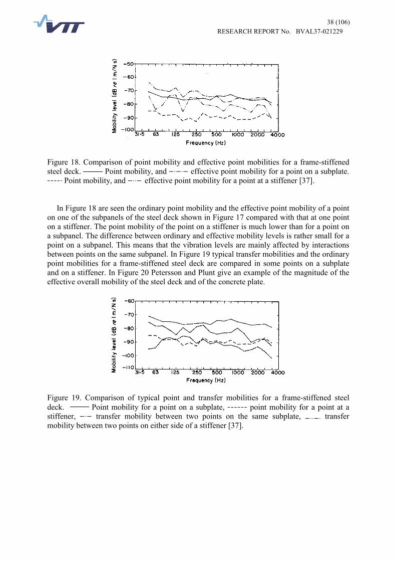
Figure 18. Comparison of point mobility and effective point mobilities for a frame-stiffenedsteel deck. Point mobility, and effective point mobility for a point on a subplate.
Point mobility, and effective point mobility for a point at a stiffener [37].
In Figure 18 are seen the ordinary point mobility and the effective point mobility of a pointon one of the subpanels of the steel deck shown in Figure 17 compared with that at one pointon a stiffener. The point mobility of the point on a stiffener is much lower than for a point ona subpanel. The difference between ordinary and effective mobility levels is rather small for apoint on a subpanel. This means that the vibration levels are mainly affected by interactionsbetween points on the same subpanel. In Figure 19 typical transfer mobilities and the ordinarypoint mobilities for a frame-stiffened steel deck are compared in some points on a subplateand on a stiffener. In Figure 20 Petersson and Plunt give an example of the magnitude of theeffective overall mobility of the steel deck and of the concrete plate.
Figure 19. Comparison of typical point and transfer mobilities for a frame-stiffened steeldeck. Point mobility for a point on a subplate, point mobility for a point at astiffener, transfer mobility between two points on the same subplate, transfermobility between two points on either side of a stiffener [37].

39 (106)RESEARCH REPORT No. BVAL37-021229
Figure 20. Effective overall mobility level for a stiffened steel deck and a concreteplate [37].
Petersson and Plunt investigated typical relations between magnitudes of point and transfermobilities making measurements of a large diesel generator (see Figure 21) and a shipstructure (see Figure 22) [38]. The double-bottom structure under measurements was thefoundation structure on board a ship for the same type of diesel generator set. Themeasurement method was described in [37], [39]. They observed from measurements on shipfoundation models that the ordinary point mobility seems to be determined by the staticstiffness of the excited substructure when the frequency is below the first resonance frequencyof this structure. Above the first resonance frequency the effect of the characteristic mobilityis seen. Then the ordinary point mobility is the mobility of the corresponding infinite systemadded with the effect of resonances.
Figure 21. Sketch showing the diesel generator. Examples of measurement and excitation
positions are marked by and respectively [38].

40 (106)RESEARCH REPORT No. BVAL37-021229
Figure 22. Sketch showing the double-bottom structure. Examples of measurements andexcitation positions are marked by and x respectively [38].
Figure 23. Examples of the ordinary point mobility for the diesel generator baseplate,measured in the vertical direction [38].
In Figure 23 are shown some measured point mobilities in the vertical direction for thediesel generator baseplate in one-third octave bands with centre frequencies from 50 Hz to3 200 Hz. From this Figure it can be noticed that the curve resembles the behaviour of astiffness-controlled system in the frequency range from 50 Hz to 500 Hz [38]. After the firstnatural frequency of the subplates between the vertical stiffeners and upwards the resonantsubplate response is observed in the mobility curve [38].

41 (106)RESEARCH REPORT No. BVAL37-021229
Figure 24. , ...., Comparison of transfer mobilities and an ordinary pointmobility, measured in the vertical direction on a diesel generator baseplate [38].
Above the frequency 50 Hz the typical transfer mobilites are lower than the ordinary pointmobility, see Figure 24. The difference is large in the frequency range where the mobilitycurve is dominated by the stiffness of the subplate excited [38]. In the frequency region wherethe subplates resonate the transfer and ordinary mobilities are almost of the same magnitude.
For the double-bottom structure the comparison of typical transfer mobilities and pointmobility is given in Figure 25. It is seen that the transfer mobilities are much smaller than theordinary point mobility in magnitude. The measurement results that Petersson and Pluntobtained for a diesel generator baseplate and for the double-bottom show that the transfermobilities between contact points are smaller than ordinary point mobilities if the contactpoints are separated at least by one stiffener between them [38].
Figure 25. , , .... Comparison of transfer mobilities and ordinary point mobility,measured in the vertical direction on the bedplate of a diesel engine foundation [38].
5.2 Applications of mechanical mobility measurementsApplications were mobility measurements are used include [21]: a) prediction of the dynamicresponse of structures to known or assumed input excitation; b) determination of the modal
42 (106)RESEARCH REPORT No. BVAL37-021229
properties of a structure, e.g., natural frequencies, mode shapes and damping ratios; c)prediction of the dynamic interaction of interconnected structures; d) checking of the validityand improvement of the accuracy of mathematical models; and e) determination of dynamicproperties, e.g., the complex modulus of elasticity of materials.
6 Analysis of mechanical systems6.1 Impedance and mobility of a system of elementsThe mechanical impedance or mobility of a system of connected elements at a point ofinterest can be calculated using Eqs. (34) through (37) and the properties of ideal mechanicalelements presented in Table 4. Generally this results in a complex impedance or mobilityfunction which represents an equivalent system for the original system of connected elements.This equivalent system has same dynamic characteristics as the original system. According toEq. (35) complex impedance represents parallel-connected elements from which the real partrepresents a purely resistive element and the imaginary part a purely reactive element. Acomplex mobility represents according to Eq. (36) series connected elements from which thereal part represents a purely resistive element and the imaginary part a purely reactiveelement. These two elements of an equivalent system need not to be the ideal resistance,spring or mass. For instance the resistance may vary with frequency and the reactance maybehave springlike, masslike or even be zero depending on frequency. The characteristics ofreal physical elements may be nonlinear and all elements have some mass, and at very highfrequencies when the wavelength becomes comparable with the element dimensions the wavephenomena may arise [36].
Table 4. Impedance and mobility of ideal lumped elements, parallel and series connectedelements.
Ideal mechanical elementor system
Impedance[(N.s)/m]
Mobility[m/(N.s)]
massmiω m
imi ωω
−=1
resistancec 1/c
springωωik
ik −=
kiω
parallel connected elements�
=
=n
iiZZ
1p �
=
=n
i iYY 1p
11
series connected elements�
=
=n
i iZZ 1s
11�
=
=n
iiYY
1s

43 (106)RESEARCH REPORT No. BVAL37-021229
6.2 Kirchhoff´s LawsKirchhoff´s Laws:1) The sum of all the forces iF which act at a connection point of elements is zero
0=�n
iiF . (88)
2) The sum of the relative velocities iv around a closed loop of series-connected elements iszero
0=�n
iiv . (89)
6.3 Superposition theoremSuperposition theorem: The response at a point of a mechanical system formed by linearbilateral elements can be calculated summing the response to each vibration source at a timewhen the other sources are not supplying energy but they are taken into account by theirinternal impedances in the mechanical system.
The superposition method is applicable for instance when there are several vibrationsources in a system to be analyzed.
6.4 Reciprocity theoremReciprocity theorem in acoustics may be stated as follows [23, p. 550]: "If a force 1F thatacts at a point 1P produces a velocity 12v at point 2P , then this same force )( 21 FF = acting atthe point 2P will produce at point 1P the velocity 1221 vv = . Thus, the ratio of the excitingforce to the observed velocity remains the same if the excitation and observation points areinterchanged, provided also that the direction in which the force acts in each case is the sameas that in which the velocity is measured in the other case." Reciprocal measurements can beused e.g. for the measurement of transfer functions in linear mechano-acoustical systems [25].
6.5 Thévenin´s equivalent circuitThévenin´s equivalent circuit: A mechanical circuit formed by linear bilateral elements,which contains vibrational force sources and which produces an output to a load impedance atsome attachment point at any particular frequency, can be replaced at that frequency by asingle constant frequency vibrational force source cF in parallel with the internal impedance
iZ of the circuit connected to the load [36].
The force cF , called clamped force, represents the transmitted force by the attachmentpoint when it is connected to an infinitely rigid structure (see Figure 26) [36]. The internalimpedance iZ of the circuit can be determined from the circuit when the force source is

44 (106)RESEARCH REPORT No. BVAL37-021229
removed from it. When there is no load at the attachment point, then the free velocity fv canbe measured and icf / ZFv = .
When the point b is attached to a rigid structure, there is no motion at the impedance 3Z ,which is why it is omitted in the Figure 26 b). The impedances 1Z and 2Z are connected inparallel in the Figure 26 b) and their total impedance is obtained from Eq. (35). Using theKirchhoff´s first law which states that the sum of the node forces is zero one obtains at thepoint a that the force )( 21a ZZvF += . So the velocity )/( 21a ZZFv += and the clampedforce transmitted by point b is )/( 2122ac ZZFZZvF +== . The internal impedance of thecircuit seen at the point b in Figure 26 c) is calculated using Eqs. (35) and (37) as
213i 11
1ZZ
ZZ+
+= . Thus the parameters needed for the Thévenin´s equivalent circuit
given in Figure 26 d) are determined using the known values of impedances and force.
� � � � �
�� ��
��
�
� � � � �
��
��
�
��� ��
��
�
���
��
�
�� ��
�����
��
�� ��
�� ��
��
�� �
Figure 26. A circuit formed by mechanical elements: a) element impedances 1Z , 2Z , and 3Zincluding vibrational force source F and the connection point b for a load impedance LZ , b)
cF is the constant force transmitted to a rigid immovable structure when the point b isclamped to it, c) the circuit for the determination of the internal impedance iZ of theThévenin´s equivalent circuit when the force source F is removed from the original circuitdescribed in a), d) the Thévenin´s equivalent circuit, e) the Thévenin´s equivalent circuitexerting the force bF and velocity bv to a load impedance LZ , and f) the Norton´s equivalentcircuit comprising of a velocity source fv in series with an internal impedance iZ isconnected to a load impedance LZ at the point b exerting the force bF and generating thevelocity bv , adapted from [36].
When the load impedance LZ is connected to the circuit at the point b (see Figure 26 e))the velocity bv and the force bF exerted to the load impedance can be calculated as follows:using the Kirchhoff´s first law which states that the sum of the node forces is zero one obtainsat the point b )( Libc ZZvF += . And solving for velocity one obtains

45 (106)RESEARCH REPORT No. BVAL37-021229
Li
cb ZZ
Fv
+= . (90)
The force at the point b is then Lbb ZvF = or
bicLi
Lcb Z
vZFZ
ZFF −=
+= . (91)
The force and velocity at point b can be calculated for any load impedance LZ from Eqs. (90)and (91).
6.6 Norton´s equivalent circuitA mechanical system of linear and bilateral elements containing vibration sources and anoutput connection for load impedance can be analyzed using Norton´s equivalent circuit. Atany particular frequency this replaces the circuit of mechanical elements by a single constant-velocity vibration source fv in series with internal impedance iZ . Norton´s equivalent circuitis the counterpart of the Thévenin´s equivalent circuit. It depends on the system to beanalyzed which of these is easier to apply, the series equivalent or the parallel equivalentrepresentation of source and internal impedance. The clamped force used in the Thévenin´sequivalent circuit is obtained easily from the free velocity and the internal impedance as
ifc ZvF = .
For the mechanical circuit presented in Figure 26 a) the Norton´s equivalent circuit can bedetermined as follows: The free velocity fv needed at the load connection point b can bedetermined with the aid of Figure 26 a) applying the Kirchhoff´s first law at the points a and band denoting fb vv = , then
f2a21 )( vZvZZF −+= ,
f32a2 )(0 vZZvZ ++−= .These equations are solved for fv
323121
2f ZZZZZZ
FZv
++= .
The internal impedance of the circuit seen at the point b in Figure 26 c) is calculated using
Eqs. (35) and (37) as 21
3i 111
ZZZZ
++= . Figure 26 f) shows the Norton´s equivalent
circuit connected to the load impedance LZ at the point b. The elements are connected inseries and transmit the same force bF which is obtained with the mobility or impedance ofelements using Eq. (36) for the series connected mobilities as
Li
Lif
L
f
L
fb Z11 Z
ZZvZZ
vYY
vF
ii +=
+=
+= . (92)
The velocity at the point b is obtained from

46 (106)RESEARCH REPORT No. BVAL37-021229
Li
Lf
Li
if
L
bb Z YY
YvZ
ZvZF
v+
=+
== .(93)
So the force and velocity at the connection point b can be determined for any load mobilityLY (load impedance LZ ) in terms of the constant free velocity fv and the internal mobility iY
(impedance iZ ) from the Norton´s equivalent circuit as shown above.
6.7 Analysis methodsAs a result of an analysis of a mechanical system using impedance methods one obtains theforces acting on the elements forming the system and the velocities of their connection points.Many other quantities can be derived from these quantities e.g. displacement and accelerationof a sinusoidal vibration [36].
Kirchhoff´s force law at a point Eq. (88) allows one to write down simultaneous equationsfor the determination of all forces and velocities in a system of mechanical elements. Usuallythis is made for each connection point of elements (force node) in terms of impedances andvelocities. At a connection point of elements there is a same velocity compared to a stationaryreference point.
Instead the Kirchhoff´s velocity law around a loop Eq. (89) allows one to write downvelocity equations for each independent mechanical circuit loop in terms of forces andmobilities. This method can be applied in the analysis of series-connected elements.
6.8 Example of analysisThe general laws of circuit analysis are applied in a practical example to see how they work inpractise. Determine the velocities of all the connection points and the forces, which act on theelements in the system of Figure 27. There are two velocity sources 1v and 6v of knownstrength operating at the same frequency but in opposite phase.
����
� ��
�
�
��
�� ��
� !�
!�
!�
�
�� ���
��
�
��
��
����
" � � " � �
Figure 27. A mechanical system with two vibration sources 1v and 6v of known strengthoperating at the same frequency but in the opposite phase and seven impedances 71 ... ZZ[36].

47 (106)RESEARCH REPORT No. BVAL37-021229
Solutions (see [36]):A: Using Kirchhoff´s force law (Eq. (88) let us first write down a force equilibrium
equation at each connection point except at points a and e.At the point b: 0321 =−− FFF . This can be expressed with the aid of velocities andimpedances remembering that relative velocity over the ends of an element times impedanceis force ( FZv =rel ) as
0)()()( 442232121 =−−−−− ZvvZvvZvv . (a)
At the point c: at the connection point of two series elements the same force is acting on bothelements, thus 022 =− FF . With the aid of velocities and impedances one gets
0)()( 343232 =−−− ZvvZvv . (b)
At the point d: 05432 =−−+ FFFF . With the aid of velocities and impedances and notingthat 6v is (+) because there is a 180º phase difference compared to 1v one gets
0)()()()( 654564442343 =−−+−−+− ZvvZvvZvvZvv . (c)
At the point f: 055 =− FF . With the aid of velocities and impedances one obtains
0)( 75654 =−− ZvZvv . (d)
From the above four equations the four unknown velocities 2v , 3v , 4v , and 5v can be solved.With the obtained velocities the forces are calculated from
1211 )( ZvvF −= 3432322 )()( ZvvZvvF −=−=
4423 )( ZvvF −= 5644 )( ZvvF +=
756545 )( ZvZvvF =−=
B: The method of node forces, rule: At each connection point with a common velocity(force node), equate the force generators to the sum of the impedances connected to that nodemultiplied by the velocity of that node minus the impedances multiplied by the velocities oftheir other connection points. Using this rule the equations of solution A can be rewritten inthe form (see Figure 27)
4432242111 )( vZvZvZZZZv −−++= . (a´)4333222 )(0 vZvZZvZ −++−= . (b´)
5646543332456 )( vZvZZZZvZvZZv −++++−−=− . (c´)57646 )(0 vZZvZ ++−= . (d´)
C: Using Kirchhoff´s law (89) for loop velocities to be zero one can write a velocityequation in terms of forces and velocities around a closed loop. One needs as many loops asthere are unknowns to be solved. From Figure 27 one sees that

48 (106)RESEARCH REPORT No. BVAL37-021229
213 FFF −= and 415 FFF −= .
Loop (1) equation:
0)()( 421322 =−−+ YFFYYF . (e)
The minus sign of the second term takes into account that the loop goes across element 4 in adirection opposing the direction of the force direction shown in the Figure 27.
Loop (2) equation:
0))(( 7641654 =+−−− YYFFvYF . (f)
Loop from A to B along the upper branch: Notice that the velocities are relative velocities( FYv = ) across the elements, thus the first term is )0( 1v− and the last one )0( 1 −− v owingto the sign rule
0)0()()0( 654322111 =−−++++− vYFYYFYFv . (g)
Solving the Eqs. (e), (f), and (g) one obtains the unknown forces 1F , 2F , and 4F . The otherforces are obtained from 213 FFF −= , and 415 FFF −= . The velocities are obtained from
1112 YFvv −= , 2223 YFvv −= , 4324 YFvv −= , and 755 YFv = .
A numerical example: calculate the velocities and forces in the previous example using thevalues without SI units: v1 = 1, v6 = 2; Z1 = 1, Z2 = 2, Z3 = 3, Z4 = 4, Z5 = 5, Z6 = 6, and Z7 = 7.
Solution:A: After inserting the values given into the Eqs. (a), (b), (c), and (d) one obtains four
simultaneous equations
��
�
��
�
�
��
�
��
�
�−
=
��
�
��
�
�
��
�
��
�
�
����
����
�
−−
−−
=
����
����
�
−−
−−
01001
136006183403520427
136006183403520427
5
4
3
2
54
5432
432
432
vvvv
vvvvvv
vvvvvv
�
��
�
��
�
�
��
�
��
�
�
−−−
−
=
��
�
��
�
�
��
�
��
�
�
466,001,188,0686,0
5
4
3
2
vvvv
.
Notice that the impedance matrix is symmetric about the main diagonal. As the impedancematrix is always symmetric, this serves as a useful check for the correctness of the equations.

49 (106)RESEARCH REPORT No. BVAL37-021229
B: Inserting the given values to Eqs. (a'), (b'), (c'), and (d') one obtains
��
�
��
�
�
��
�
��
�
�
−=
��
�
��
�
�
��
�
��
�
�
����
����
�
−−−−
−−−−
=
����
����
�
−−−−
−−−−
01001
1360061834
03520427
136006183403520427
5
4
3
2
54
5432
432
432
vvvv
vvvvvv
vvvvvv
�
��
�
��
�
�
��
�
��
�
�
−−−
−
=
��
�
��
�
�
��
�
��
�
�
466,001,188,0686,0
5
4
3
2
vvvv
.
C:
��
��
�
��
��
�
=��
��
�
��
��
�
���
���
�
−−
=���
���
�
−−
320
2,0833,015095,003095,000833,125,0
2,0833,05095,003095,0
00833,125,0
4
2
1
421
41
21
FFF
FFFFF
FF
�
��
��
�
��
��
�
=��
��
�
��
��
�
949,4389,0686,1
4
2
1
FFF
.
and the other forces are obtained from:
297,1389,0686,1213 =−=−= FFF263,39949,4686,1415 −=−=−= FFF .
The velocities can be calculated with the solved forces and known mobilities (1/Z):11 =v was known
686,0)1/1(686,111112 −=⋅−=−= YFvv881,0)2/1(389.0686,02223 −=⋅−−=−= YFvv
01,1)4/1)(389,0686,1(686,0)( 42124324 −=−−−=−−=−= YFFvYFvv466,0)7/1(263,3755 −=⋅−== YFv
26 =v was known.

50 (106)RESEARCH REPORT No. BVAL37-021229
7 Impedance and mobility parameters7.1 Impedance parametersIn a generalized two-connection system shown in Figure 28 a force 1F is applied to excite theinput and as a result a velocity 1v is obtained. The ratio 11 / vF is called the input impedance.If instead a force 2F is applied to excite the output, then a velocity 2v results. The ratio
22 / vF is called the output impedance. When the force 1F is applied to the input and theoutput velocity 2v results, then the ratio 21 / vF is the reverse transfer impedance. When theforce 2F is applied to excite the output and the velocity 1v results, then the ratio 12 / vF iscalled the forward transfer impedance. These definitions can be
# � � $ �����
�� ��
� % & $ ' & $ % & $
Figure 28. Generalized two-connection system [36].
applied to get the impedance parameters [36]:
021
111
==
vvF
Z , (94)
where 11Z is the input impedance under the condition 02 =v meaning that the output isclamped (or blocked), i.e., connected to a rigid point. Similarly one gets the output impedance
012
222
==
vvF
Z . (95)
The reverse transfer impedance 12Z is
012
112
==
vvF
Z , (96)
where the input is clamped and 1F is the force required to keep the input velocity 01 =v . Theforward transfer impedance 21Z is
021
221
==
vvF
Z , (97)

51 (106)RESEARCH REPORT No. BVAL37-021229
where the output is clamped and 2F is the force required to keep the output velocity 02 =v .
A two connection passive system can be represented by a black box, which is attached toan inertial reference (see Figure 29). If the elements in this system are linear and bilateral,then the relationship between the forces and velocities at the connection points
� � � ( � � � �
� � � � � � $ �����
��
�� ��
�� ��
�� �
Figure 29. A mechanical system described as a black box, which has two connections andwhich is attached to an inertial reference. The vibration source is presented by a Nortonequivalent system having free velocity fv and internal mobility iY . The load is presented byits mobility LY . The forces and velocities at connection points 1 and 2 are noted by 11 , vF and
22 , vF , respectively [35].
1 and 2 can be expressed as [36]:
2121111 vZvZF += , (98)
2221212 vZvZF += , (99)
where the iiZ 's are the impedance parameters. When the forces and the impedance parametersare known, the velocities can be obtained by solving Eqs. (98) and (99).
7.2 Mobility parametersThe mobilities of a generalized system shown in Figure 28 are [36]:The input mobility 11Y is
021
111
==
FFv
Y , (100)
where the output is free without no restraining force, i.e., 02 =F .
The output mobility 22Y is
012
222
==
FFv
Y , (101)

52 (106)RESEARCH REPORT No. BVAL37-021229
where the input is free without no restraining force, i.e., 01 =F .
The reverse transfer mobility 12Y is
012
112
==
FFv
Y , (102)
where 1v is the velocity of the free input, 01 =F , when the force 2F is applied to excite theoutput.
The forward transfer mobility 21Y is
021
221
==
FFv
Y , (103)
where 2v is the velocity of free output, 02 =F , when the force 1F is applied to excite theinput.
The relationships between the velocities and forces of the black box system shown inFigure 29 can also be expressed using the mobility parameters iiY as [36]:
2121111 FYFYv += , (104)and
2221212 FYFYv += . (105)
When the velocities at the connection points and the mobility parameters are known, then theforces are obtained by solving the Eqs (104) and (105).
In the mechanical black box system presented in Figure 29 the vibration source isdescribed by Norton equivalent with free velocity fv and internal mobility iY and the load isgiven by its load mobility LY . The internal mobility of the vibration source and the mobilityof the load can be included with the black box mobilities by measuring or calculating themobility parameters with the load mobility LY and internal mobility iY in place. In doing sothe Eqs. (104) and (105) become [36]
212111f FYFYv +′= , (106)and
2221210 FYFY ′+= . (107)
Now the forces and velocities are considered at points 1′ and 2. The velocity at point 1′ 1vbecomes fv and the velocity 02 =v because no external force is applied. The mobility 11Y ′ is
11Y obtained from Eq. (100), and 22Y ′ is 22Y obtained from Eq. (101) with LY in place [36].The transfer mobilities are not effected by the external connections. From Eqs. (106) and(107) one obtains the forces [36]

53 (106)RESEARCH REPORT No. BVAL37-021229
21122211
22f1 YYYY
YvF
−′′′
= (108)
and
21122211
21f2 YYYY
YvF
−′′−
= . (109)
The force 2L FF = is applied to the load giving rise to load velocity L2L YFv = . The force atthe input connection point 1 is 1F , since the internal mobility iY of the vibration sourcetransmits this force and the velocity at the point 1 is 11f1 YFvv −= .
8 Four-pole parameters of mechanicalsystems
8.1 TheoryThe mechanical system (see Figure 30) can be described with the so called mechanical four-pole parameters jiα appearing in the equations between the input force 1F and velocity 1vand the respective output force 2F and output velocity 2v as [34]
2122111 vFF αα += , (110)
2222211 vFv αα += . (111)
� �
� � ) � � � � � �
* � + � � � $ � � �
, � - � � � � � � � � $ �
� �
Figure 30. Four-pole parameter notation, adapted from [34], [35].
The four-pole parameters are defined for a particular system and they do not depend onwhat proceeds or what follows the system. This property allows the calculation of propertiesof a complicated system comprised of many mechanical elements. The system can be acombination of lumped, linear, mechanical elements like masses, springs, and resistances. Thesystem can be made up also of linear, distributed parameter systems comprizing, e.g., beamsand plates [34].

54 (106)RESEARCH REPORT No. BVAL37-021229
The four-pole parameters can be defined from equations [34], [35]:
0 ,
0 22
112
22
111 =
==
=Fv
FvF
F αα ,(112)
0 ,
0 22
122
22
121 =
==
=Fv
vvF
v αα . (113)
In these equations the subscript 02 =v means that the output terminal pair is clamped, and thesubscript 02 =F means that the output terminal pair is free (unrestrained).
According to the reciprocity theorem in a network the transfer impedance or mobilitybetween any two terminal pairs is independent of which terminal pair is taken as the input oroutput; thus one obtains [35]
011
2
022
1
==
=FF v
FvF (114)
or
011
2
022
1
==
=vv F
vFv
. (115)
Applying the reciprocity theorem the four-pole Eqs. (110) and (111) can be inverted toyield the equations [35]
1121222 vFF αα += (116)and
1111212 vFv αα += , (117)
where use has been made of the relation [35]
1)( 21122211 =−=∆ αααα . (118)
For a symmetrical system it does not matter which terminal is taken to be input or output, thus[35]
2211 αα = . (119)

55 (106)RESEARCH REPORT No. BVAL37-021229
8.2 Four-pole parameters of a series connectedsystem
The four-pole parameters of the two elements connected in series (see Figure 31) can beobtained considering that the output of the thirst element is the input of the second element.This can easily been made using matrix notation as follows [34], [35]: using Eqs. (110) and(111) one obtains for element number 1
� �
� � ) � � � � � � . � � � $ � �
�
� � � � �. � � � $ � �
� � �� � ��
Figure 31. Series connected mechanical elements.
��
���
���
���
�
′′′′
=��
���
�
2
2
2221
1211
1
1
vF
vF
αααα (120)
and for element number 2
��
���
���
���
�
′′′′′′′′
=��
���
�
3
3
2221
12112
2 vF
vF
αααα
. (121)
Then inserting the Eq. (121) into (120) one obtains
��
���
���
���
�
′′′′′′′′
��
���
�
′′′′
=��
���
�
3
3
2221
1211
2221
1211
1
1
vF
vF
αααα
αααα
. (122)
Then after matrix multiplication one obtains
��
���
���
���
�=��
���
�
3
3
2221
1211
1
1
vF
vF
ββββ
. (123)
The final four-pole parameters expressed with the aid of the original parameters of the twoconnected elements are [35]
��
���
�
′′′+′′′′′′+′′′′′′+′′′′′′+′′′
=��
���
�
2222122121221121
2212121121121111
2221
1211
αααααααααααααααα
ββββ
. (124)
For a system of n elements one obtains [35]
��
���
�
��
��
��
���
���
���
�
′′′′′′′′
��
���
�
′′′′
=��
���
�
+
+
1
1
2221
1211
2221
1211
2221
1211
1
1
n
nnn
nn
vF
vF
αααα
αααα
αααα
� . (125)

56 (106)RESEARCH REPORT No. BVAL37-021229
8.3 Four-pole parameters of a parallel connectedsystem
Consider that the parallel connected four-pole elements move so that their input velocities atthe common input junction are equal to 1v and their output velocities, respectively, are equalto 2v . The force at the input junction is equal to the sum of the input forces of the individualfour-pole elements. The output force is also the sum of the forces of the individual fore-poleelements, which are connected parallel as shown in Figure 32 A. The equivalent four-poleparameters of the combined system can be obtained from equations [36]
���===
===
==−==
n
ii
in
ii
n
ii
i
CBA
BC
BB
BAC
BA
1)(
21
)(22
1)(
211)(
21
)(11
22211211
. ,1, where
,,1,,
αα
ααα
αααα(126)
� � � � /" � �
� � � � /" � �
� � � � /" � �
�
�
� �
� �
� � �
� � �� � � � /
� �
� �
Figure 32. Parallel connected elements in the four-pole method [36].
8.4 Four-pole parameters of lumped systems
8.4.1 Mass
A mass can be considered as a rigid body, so the velocities in the input and output in the four-pole model (see Figure 30 for positive directions) for a mass are equal 21 vv = . From Newton´slaw and assuming sinusoidal time dependence ( tie ω ) one obtains [34]
212121 mvimvidtdvmdtdvmFF ωω ====− .
Using these relationships one can write the four-pole Eqs. (110) and (111) for a mass as
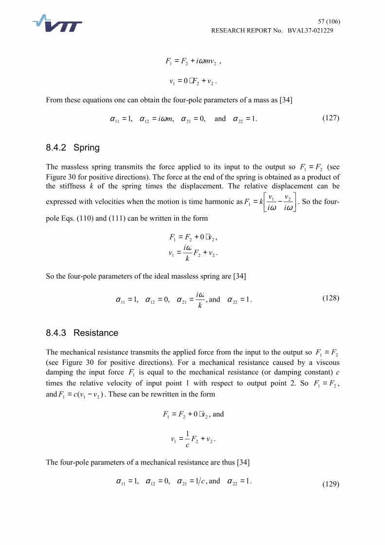
57 (106)RESEARCH REPORT No. BVAL37-021229
221 mviFF ω+= ,
221 0 vFv +⋅= .
From these equations one can obtain the four-pole parameters of a mass as [34]
.1and ,0,,1 22211211 ==== ααωαα mi (127)
8.4.2 Spring
The massless spring transmits the force applied to its input to the output so 21 FF = (seeFigure 30 for positive directions). The force at the end of the spring is obtained as a product ofthe stiffness k of the spring times the displacement. The relative displacement can be
expressed with velocities when the motion is time harmonic as ��
���
� −=ωω iv
iv
kF 211 . So the four-
pole Eqs. (110) and (111) can be written in the form
221 0 vFF ⋅+= ,
221 vFk
iv += ω .
So the four-pole parameters of the ideal massless spring are [34]
1and ,,0,1 22211211 ==== αωαααk
i . (128)
8.4.3 Resistance
The mechanical resistance transmits the applied force from the input to the output so 21 FF =(see Figure 30 for positive directions). For a mechanical resistance caused by a viscousdamping the input force 1F is equal to the mechanical resistance (or damping constant) ctimes the relative velocity of input point 1 with respect to output point 2. So 21 FF = ,and )( 211 vvcF −= . These can be rewritten in the form
221 0 vFF ⋅+= , and
2211 vFc
v += .
The four-pole parameters of a mechanical resistance are thus [34]
1and ,1,0,1 22211211 ==== αααα c . (129)

58 (106)RESEARCH REPORT No. BVAL37-021229
8.4.4 Parallel spring and resistance
In a system of parallel-connected spring and resistance (see Figure 33) the equations forforces and velocities are [35]
�� ) �� �� ) ���
�
Figure 33. Parallel connected spring and resistance.
21 FF = (130)and
221 vFv += ∗κ , (131)where
[ ] 1)/( −∗ += cjk ωκ . (132)Thus the four-pole parameters are
∗==== καααα 21122211 ,0 ,1 , (133)and
[ ]��
���
�
��
�
�
��
�
�
+=�
�
���
���
���
�=��
���
�∗
2
2
2
2
1
11
)/(1
01
101
vF
kcjkj
vF
vF
ωω
κ.
(134)
8.4.5 Dynamic absorber
One can apply the method of series connected lumped elements to get the matrix equation fora dynamic absorber shown in Figure 34
�� ) �� �� ) ���
�
��� ) ��
Figure 34. Dynamic absorber.
��
���
���
���
�
+=�
�
���
���
���
���
���
�=��
���
�∗∗∗
3
3
3
3
1
1
11
101
101
vF
mjmj
vFmj
vF
κωκωω
κ. (135)
Normally the dynamic absorber is unterminated. In that case the transfer impedance0/ 33T == vFZ and the driving-point impedance inZ is

59 (106)RESEARCH REPORT No. BVAL37-021229
∗+==
κωω
mjmj
vF
Z11
1in , (136)
where ∗κ is obtained from Eq. (132).
8.4.6 Dynamic absorber in a mechanical system
A dynamic absorber is attached to a mechanical system in Figure 35. For the mechanicalsystem one can write the equation [35]
�� ) ��
�� ) ��
�
�
�
�� ) ��
, � - � � � � �
� � � $ �
��� � )" ��� �
Figure 35. Mechanical system with a dynamic absorber attached [35].
��
���
���
���
�=��
���
�
3
3
2221
1211
2
2
vF
vF
αααα
. (137)
The force balance equation gives
2in21 vZFF += , (138)
where inZ is the driving-point impedance of the dynamic absorber given in Eq. (136).Because 21 vv = , one can write in matrix form [35]
��
���
���
���
�=��
���
�
2
2in
1
1
101
vFZ
vF
. (139)
Inserting the Eq. (137) into Eq. (139) one obtains
��
���
���
���
���
���
�=��
���
�
3
3
2221
1211in
1
1
101
vFZ
vF
αααα
, (140)
and after matrix multiplication
��
���
���
���
� ++=�
�
���
�
3
3
2221
22in1221in11
1
1
vFZZ
vF
αααααα
. (141)

60 (106)RESEARCH REPORT No. BVAL37-021229
9 Characterization of structure-borne soundsource
9.1 IntroductionAt the design stage the engineer is often asked to evaluate the resulting vibration and soundlevel the machine will produce. For airborne sound the source-transmission path-receivermodel is well established and it gives good results. A similar approach has not been able todevelop for structure-borne sound. There is a fundamental problem how to characterizemachines as structure-borne sound sources. When a source is connected to a receivingstructure the coupling between these depends on both the source and receiver structuralcharacteristics and the excitation of the source. So the combined system can not be describedonly with the source characteristics.
9.2 Complex power transmissionThe complex transmitted power Q in the one contact point to the receiving structure isobtained from [23]
∗∗ ==+= r21
r21 vFvFiSPQ �
�
�
�
, (142)
where F�
is the complex amplitude of the force applied on the receiving structure and rv� isthe complex amplitude of the resulting velocity at the same contact point. The real part P ofthe complex power Q, where force and velocity are in phase, is the active power flowing fromthe source into the receiving structure where it propagates further. The imaginary part, thereactive power S, where force and velocity are 2/π out of phase, goes back and forth throughthe contact point. Using the point mobility rY of the receiving structure at the contact pointthe complex power can be written in the form
r2
r
2
21 ~ YFYFQ ==
�
, (143)
where F~ is the rms-value of the complex force, or equivalently using velocity
r2r
2r
r2r
2r
21
~Y
Yv
YY
vQ ==
�
, (144)
where r~v is the rms-value of the complex velocity at the contact point. From Eq. (143) one
can see that the complex power Q and the driving-point mobility rY of the receiving structureare in same phase. Petersson and Gibbs [40] introduce two quantities relevant to the powertransmission:
rr 2 YQv =�
(145)and
[ ]QRe=P . (146)
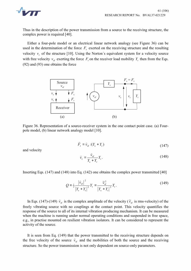
61 (106)RESEARCH REPORT No. BVAL37-021229
Thus in the description of the power transmission from a source to the receiving structure, thecomplex power is required [40].
Either a four-pole model or an electrical linear network analogy (see Figure 36) can beused in the determination of the force rF exerted on the receiving structure and the resultingvelocity rv of the structure [10]. Using the Norton´s equivalent system for a velocity sourcewith free velocity sfv exerting the force rF on the receiver load mobility rY then from the Eqs.(92) and (93) one obtains the force
# � & � � � � �
� � � 0 �
" �
� �
� �
� �
� �
� � �
� � � 1 � � �
� �
� �� � � �
" � �
Figure 36. Representation of a source-receiver system in the one contact point case. (a) Four-pole model, (b) linear network analogy model [10].
)/( rssfr YYvF += �
�
(147)and velocity
rrs
sfr Y
YYv
v+
=�
� . (148)
Inserting Eqs. (147) and (148) into Eq. (142) one obtains the complex power transmitted [40]
r2rs
2sf
r2rs
2sf
21
~Y
YYv
YYY
vQ
+=
+=
�
. (149)
In Eqs. (147)-(149) sfv� is the complex amplitude of the velocity ( sf~v is rms-velocity) of the
freely vibrating source with no couplings at the contact point. This velocity quantifies theresponse of the source to all of its internal vibration producing mechanism. It can be measuredwhen the machine is running under normal operating conditions and suspended in free space,e.g., in practise mounted on resilient vibration isolators. It can be considered to represent theactivity of the source.
It is seen from Eq. (149) that the power transmitted to the receiving structure depends onthe free velocity of the source sfv� and the mobilities of both the source and the receivingstructure. So the power transmission is not only dependent on source-only parameters.

62 (106)RESEARCH REPORT No. BVAL37-021229
9.2.1 Constant velocity and constant force source
A constant velocity or a constant force source are the two theoretical idealizations which arevery seldom encountered. In practice machine and structural design is based on staticrequirements which lead to structural elements of similar proportions, e.g., thicknesses [40].Consider a situation where a source is attached at a single point and the motion is consideredin only one direction of motion. If the source mobility sY is very small compared to thereceiver mobility rY ( rs YY << ) then the Eq. (149)
r2rs
2sf
r2rs
2sf
21
~Y
YYv
YYY
vQ
+=
+=
�
reduces to [40]
r2r
2sf
21 Y
Y
vQ
�
=
showing that in this case the complex power transmitted is independent of the mobility of thesource. In theory this kind of situation is encountered when a solid massive machine ismounted on a thin foundation plate. Then the velocity at the contact point is the free velocity
sfv measured when there are no contacts between the machine and its environment and whenthe machine is running under normal load. This extreme situation describes the so-calledconstant velocity source [40].
If instead the source mobility sY is very large compared to the receiver mobility rY thenEq. (149) reduces to [40]
r2s
2sf
21 Y
Y
vQ
�
=
and then the force at the contact point becomes invariant (constant). This theoretical situationis encountered when a machine with large mobility is mounted on a thick floor [40].
9.2.2 Transmission loss of elastic elements
Between the source and receiver there are often elastic elements, called transmissionelements, e.g., chocks, vibration isolators, bolts, pipes, tubes or cables. If there is an elasticelement between a simple source and a receiver, then the velocities at its top and bottom ends,
1v and 2v respectively, can be written as [40]
1221111 YFYFv��
� += , (150) and
2222112 YFYFv��
� += , (151)
where iiY are the driving-point mobilities and jiY the transfer mobilities.
It can be shown that the transmitted complex power from source to the receiver is obtainedfrom [40]

63 (106)RESEARCH REPORT No. BVAL37-021229
2211222r11s
221
2rs
0))(( YYYYYY
YYYQQ
−++
+= , (152)
where 0Q is from Eq. (149) calculated complex power without the transmission element inplace, and the transmission efficiency t can be defined as ([10] in [40])
2211222r11s
221
2rs
))(( YYYYYY
YYYt
−++
+= . (153)
One sees from Eq. (153) that in addition to element mobilities both the source and receivermobilities will effect on the transmission efficiency. This differs from the force ordisplacement transmissibility [41] which considers only one field variable at a time [40].
An approximate expression for the transmission efficiency when the element mobilities arelarger that the source and receiver mobilities is [40]
221122211
2212
rsYYYY
YYYt
−+=′ . (154)
In the approximate Eq. (154) for t ′ the second factor is the square of the ratio (transferimpedance) of force at a blocked end to the velocity at the excited end [40]. In the generalcase its mobility matrix describes the transmission element
��
���
�=2221
1211T YY
YYY . (155)
When elements are linear, passive and bilateral then the reciprocity principle applies and2112 YY = . If the elements are in addition symmetrical then 2211 YY = .
9.2.3 Source descriptor and coupling function
9.2.3.1 One-point-connected systems
For the description of the complex power transmission at one contact point from the vibrationsource to the receiving structure Mondot and Petersson [10] introduced the ratio of themagnitude of the receiver and source mobilities, sr YY=α , and the phase differencebetween these mobilities, sr φφφ −=∆ . They proposed that the source characterization can bemade with two functions: the source descriptor S describes the ability of the source to producepower and the coupling function Cf gives the proportion of this power which is manifested,defining these functions, respectively, as
∗=s
2sf
~
Yv
S , (156)

64 (106)RESEARCH REPORT No. BVAL37-021229
)1cos2/(or ,/ 22rsrs +∆+=+= ∆∗ φααα φieCfYYYYCf , (157)
where sf~v is the rms-velocity of the free source at the contact point, ∗
sY is the complexconjugate of the source mobility, and rY is the receiver mobility. The complex power in Eq.(149) can be obtained with the aid of the source descriptor and the coupling function from
SCfQ = . (158)
The source descriptor S has the units of power and it depends only on source data, thevelocity sfv of the free source and the source mobility at the contact point sY . The couplingfunction Cf is a function of the source and receiver mobilities at the interface and it describesthe dynamic properties of these coupled structures at the contact point. For any phasedifference between the source and receiver mobilities the level of the coupling function attainsits maximum when the magnitudes of these mobilities are equal. When the magnitude ratio iskept constant, then the largest coupling is obtained for the largest phase difference [10]. Themagnitude of the coupling function is low when the mobilites are largely different inmagnitude. Under these conditions the mobilities are called unmatched and the transmissionis essentially independent of the phase difference between the source and receiver monbilities[10]. When the mobilites are nearly of equal magnitude, the magnitude of the couplingfunction can be high depending on the phase difference. Under these conditions the mobilitiescan be called matched and the power transmission is dependent both on the source descriptorand the mobility matching at the interface [10].
The active power P, the real part of the complex power Q, is the quantity, which iscontrolled when the structure-borne sound power transmission or propagation needs to bereduced. The active power P can be written using the source descriptor S and the couplingfunction Cf in the form
)sinsincos(cos ss φφφφ ∆−∆= CfSP . (159)
When the source, source descriptor, is known the power transmission is obtained using thecoupling function. The most favourable contact point can be selected estimating the minimumgiving coupling function. One has to design sources and receivers so that lightly dampedvibration modes can be avoided, thus the phase difference of the source and receivermobilities can be kept small. When lightly damped resonant structures are used then thecomparable magnitudes of the mobilities of the source and receiving structure causeconsiderable transmission of vibration and power [10].
The source descriptor has some distinct properties: It is a function of the source involvingonly source variables. It has the units of power, which enables the comparizon of differentcomponents of motion. In one-point uni-directional system both the source descriptor and thecoupling function involve only variables which are measurable when the source and thereceiver are not coupled together and therefore the prediction of the transmitted power ispossible [14].

65 (106)RESEARCH REPORT No. BVAL37-021229
9.2.3.2 Multi-point-connected systems
The characterization of machines as vibrational sources is fundamental in the control ofstructure-borne sound. The dynamic coupling between the source and receiver does not allowthe use of transmitted power in the source characterization. Some proposals have been madeto standardize the structure-borne sound emission [9] for the case when the source is stablethese include the constant force or velocity sources [23]. Theoretically in the general casethese ideas do not work. Fulford and Gibbs [14], [15], [16] have studied further the ideas ofMondot and Petersson [10] applying the source descriptor and coupling function in multi-point-connected systems.
In a general motion six degrees of freedom are possible, three translational and threerotational, and the source and the receiver can be coupled at many points. In the analysis ofthis system coupling between all points and all components of motion has to be taken intoaccount. Using the source mobility matrix, [ ]sY , the receiver mobility matrix, [ ]rY , and theforce ratio vector, { }n
imj FF / , the transmitted power can be obtained from [14]
[ ] { } [ ] { }[ ] { }{ }n
imjn
imj
ni
mj
nisfn
i FFYFFYFFY
vP /Re
//2
)(r2
rs
2
+= . (160)
The Eq. (160) shows the complexity of the determination of power transmission in multi-point-connected systems [14]: For N connection points the receiver and source matrices are
NN 66 × matrices of complex and frequency dependent elements. It is difficult to comparedifferent mobility terms and compare the significance of the source and receiver mobility.Also it is difficult to see what are the dominant transmission paths of structure-borne sound.To get better understanding of the power transmitted the force ratios should be known.
Fulford and Gibbs use the concept of effective point mobility to address the problemsmentioned using the definition for point n in direction i presented in [43]
� ���≠= ≠=≠=≠=
Σ +++=N
nmm jjn
i
mjnm
ijni
nj
ijj
nnij
N
nmmn
i
minm
iinn
iinn
ii FF
YFF
YFF
YYY ,1
6
1 ,1
6
,1 ,1
, (161)
where nmijY are the transfer mobilities when force is acting at the point m and direction j to the
point n and direction i and ni
mj FF are the force ratios, respectively. The different terms in
Eq. (161) highlight the important transmission paths. The first term is the direct path, and thesecond (sum) term is due to the couplings between other points to point n in the direction ofmotion i. The third (sum) term is due to the couplings between other motion directions j anddirection i in the point n under consideration, and the fourth (sum) term is due to couplingsfrom other points m and other motion directions than the motion direction i underconsideration.
In multi-point-connected systems the effective point mobility is analogous to the pointmobility. The source descriptor and the coupling function for a point n and in motiondirection i for a multi-point-connected system are thus analogously [14]
∗Σ= nnii
ni
ni YvS s,
2
sf, 2/ , (162)

66 (106)RESEARCH REPORT No. BVAL37-021229
2
r, s, r, s, / ΣΣΣ∗Σ += nnii
nnii
nnii
nnii
ni YYYYCf . (163)
The transmitted complex power niQ in the point n and direction i is obtained from product
ni
ni
ni CfSQ = . (164)
The real part of complex power gives the active power niP , and the total active power is
obtained by the sum of all niP . In the effective point mobility of a multi-point-connected
system there are the force ratios, and they are dependent on both the source and receiverstructures. Thus one has to predict or estimate these force ratios in some manner [14]. Theforce ratios in a receiver system came under consideration through the concept of effectivepoint mobility. In the theoretical consideration of translational forces Mondot, Petersson andGibbs used assumption that they have unity magnitude and zero phase [14]. If onlytranslational motion is considered, the effective point mobility has been estimated by [14]
�≠=
Σ +=N
nmm
nmii
nnii
nnii YYY
,1
, (165)
where only contribution of other points in the same direction is taken into account. If in alinear system the contribution from N contact points can be assumed to cancel throughsuperposition, each mobility and force ratio has different phase, and the effective pointmobility reduces to the point mobility [14]
nnii
nnn YY =Σ . (166)
This assumption is equivalent to the assumption that the contact points are uncoupled. Whentaking into account both the excitation of the source and its structural characteristics a simpleassumption is that the excitation is the free velocity of the contact points and the pointmobility of the source in these points. Thus the force at the contact points is [14]
nnii
ni
ni YvF ssf /= . (167)
A more accurate estimation needs the coupling terms between contact points, i.e., the transfermobilities, but this leads to complicated expressions for the forces and effective mobility.

67 (106)RESEARCH REPORT No. BVAL37-021229
9.2.4 Characteristic power
In a single contact point case it is assumed that a source is linear and vibrates as a result of theaction of internal forces which are independent of the attachment to any receiving structure[80]. The free velocity fsv� of the source is assumed to characterize the activity of the sourceand the mobility sY is assumed to characterize its passive properties at the contact point [80].The complex power that is transmitted through the contact point is given by Eq. (149)repeated here for clarification [80]
2srr
2
sf /~ YYYvQ +⋅= . (168)
where fs~v is the rms free velocity ( fsv� is complex amplitude), rY and sY are the receiver and
source mobility respectively.
Using the complex ratio of receiver to source mobility sr /YY=α Eq. (168) can be writtenin a dimensionless form [80]
)1(// r2cc
θαα jeSQC +== , (169)
where ∗= s2
sfc /~ YvS , rθ is the phase of the receiver mobility, and cC is the so-calledcoupling factor.
The magnitude and real part of the dimensionless power transmitted from a source of agiven phase when connected to a receiver of opposite phase is drawn in Figure 37. When thesource mobility is high in relation to the receiver mobility ( 1<<α ), the blocked mountingcondition is approximated and the power transfer is inefficient. On the other hand, when thesource mobility is low in relation to the receiver mobility ( 1>>α ), the free mountingcondition is approximated and again the power transfer is inefficient. These extreme cases oflow power transfer are shown by asymptotic lines in Figure 37. The power transfer obtains itsmaximum for any phase angle when 1=α .

68 (106)RESEARCH REPORT No. BVAL37-021229
0,001
0,01
0,1
1
10
100
0,01 0,1 1 10 100
Ratio of receiver to source mobility magnitude |α | = |Y r / Y s|
|Q| /
|Sc|
(a)
0,001
0,01
0,1
1
10
100
0,01 0,1 1 10 100
Ratio of receiver to source mobility magnitude |α | = |Yr / Ys|
Re[Q
/ |S
c|]
blocked source free source
source on mirror receiver (Yr = Ys)
(b)
Figure 37. (a) Magnitude, and (b) real part of the power via a single contact point from asource of various mobility phases to a receiver of opposite phase ( sr θθ −= ). Diagonal linesindicate blocked and free source asymptotes. Phase θ : 0; π2,0 ; π4,0 ;
π45,0 . Adapted from [7] and [80].

69 (106)RESEARCH REPORT No. BVAL37-021229
From Eq. (168) the maximum complex power is obtained when the mobilities of sourceand receiver are complex conjugate ( ∗= sr YY ) [10]
[ ] 2ss
2sfasr )Re(2/~)( YYvSYYQ ∗∗ ⋅=== . (170)
The "maximum available power" (MAP) that is transmitted from this source through itscontact point to any receiving structure is obtained from [80]
[ ] )Re(4/~)Re()(Re s2
sfasr YvSYYQ === ∗ . (171)
In Figure 37 (b) is drawn the real part of Eq. (169) for sr θθ −= , that is the MAP, for fourdifferent values of source mobility phase.
When source and receiver mobilities are equal in magnitude and phase ( sr YY = ) then fromEq. (168) is obtained [80]
)(4/1~)( s2
sfmsr∗⋅=== YvSYYQ . (172)
This is called the "mirror" power, because it is the power transmitted when the source isconnected to receiver which is a mirror image of itself [80]. The magnitude of the mirrorpower is independent of source mobility phase, whereas the magnitude of MAP depends onthe source mobility phase. For most sources, the magnitude of the mirror power is less thanthe MAP power. In a special case of a source of zero mobility phase both powers are equal[80].
The intersection point of the low mobility and the high mobility source asymptotes inFigure 37 is of interest. In this point the force is equal to the blocked force )/( ssfbl YvF �= andthe velocity is the free velocity, and power is obtained from [80]
∗⋅==== s2
sfcsfbl /1~) ,( YvSvvFFQ �� . (173)
This is four times the "mirror" power obtained from Eq. (172). Mondot and Petersson [10]call the result of Eq. (173) the source descriptor. Moorhouse introduced for this result a newterm the "characteristic power" to be able to enlarge the discussion to include also themultiple point contacts, because it differs from the characterization by Mondot and Petersson.This work was extended to multiple point and component contact also in [80].
10 Mobility functions and free velocities
10.1.1 Machine mobilities
The mount footing is typically a flat plate for a large range of machines [44]. The dynamics ofthis kind of mount can be modelled as a plate-spring-mass system (see Figure 38). The masspresents the machine body and the spring the local stiffness of the footing. The boundary

70 (106)RESEARCH REPORT No. BVAL37-021229
conditions, material and dimensions of the plate determine the stiffness. For this model thepoint mobility is obtained from [15]
Figure 38. Model of a machine mount point [15].
kmimkY ωω /)( 2−= , (174)
where m is the mass of the machine, k the local stiffness of the mount footing, and ω is theangular frequency. At low frequencies the mass term dominates the expression and in themobility curve (see Figure 39) a mass controlled region (magnitude decrease of 6 dB peroctave with a phase of 2/π− ) is seen. Thereafter at higher frequencies is seen a stiffnesscontrolled region (magnitude increase of 6 dB per octave with a phase of 2/π ). Betweenthese two regions is seen notch caused by an anti-resonance frequency determined by themass and local stiffness
Figure 39. Generalized point mobility of machine mount [15].
mk /0 =ω . (175)
After the stiffness controlled region the plate will begin to bend and its fundamentalfrequency starts the resonance controlled region, where a more detailed model is needed.
10.1.1.1 Mobility in mass controlled region
The machine can be modelled as a rigid body in the mass controlled region. If the co-ordinateaxes coincide with the principal inertia axes of the body of the machine, the mobility isobtained from [15]
)///1)(/1( 00 yyxx IxxIyymiY ++= ω , (176)

71 (106)RESEARCH REPORT No. BVAL37-021229
where 0x and 0y describe the position of the force with respect to the centre of gravity, x andy are the co-ordinates of the response point, and the moments of inertia are xxI and yyI (see[15]).
10.1.1.2 Mobility in stiffness controlled region
In the stiffness controlled region the size, material and boundary conditions of the mount platecontrol the mobility and the main body of the machine can be ignored in the analysis [15].Fulford and Gibbs consider in the analysis plate- and flange-like mount conditions (see Figure40). They also consider cantilever flanges and local plate deformation (see Figure 41).
Figure 40. Machine with a plate-like base (left) and with a flange-like base [15].
Figure 41. Machine with cantilever flanges (left) and local plate deformation [15].
10.1.1.3 Mobility in resonance controlled region
The transfer trY and point mobility ptY of the machine base are dependent on the modalinteraction in the resonance region of the mobility curve. Mode shapes and mode frequenciesdepend on the material, dimensions and boundary conditions; and the modal interactiondepends on the frequency, excitation position, reception position and material damping. Thisis why the analytical determination of the relationship pttr /YY is difficult [15].
Skudrzyk subdivided the resonance region into four frequency regions: a) low frequencies( 5>α ), b) transition frequencies ( 51 <<α ), c) high frequencies ( 1≈α ), and d) very highfrequencies ( 1≤α ). The ranges were determined by the ratio α of average modal spacing νε(rad/s) to the half-power bandwidth νηω of a mode ν given in [45] and denoted by α in [15]
vv ηωεα /= , (177)

72 (106)RESEARCH REPORT No. BVAL37-021229
where η is the material loss factor, and νω is the angular frequency of the mode ν . Thefrequencies in the regions c) and d) are not of concern as to the mobilities of machines [15].The modal spacing of a thin mount plate transversely excited is obtained from [15]
Ahc /6,3 L=νε , (178)
where Lc is the quasi-longitudinal wave speed, h plate thickness, and A plate area. From Eqs.(177) and (178) is obtained
νωηα Ahc /6,3 L= . (179)
Using values 001,0=η and upper frequency limit of 10 kHz, the plate area required tohave 1=α for a 3 mm thick plate is 1 m2 and for thicker plates the area will be larger than1 m2 [15]. This example shows that these two regions of Skudrzyk are not applicable inengineering practice. For the region b) the plate are with same assumptions will be about0,2 m2 which is of practical concern. In the low frequency region where 5>α the mobilitywill have well separated peaks. Even in this region it is not possible to predict the exactmobility spectra excluding the simplest structures. It is considered that only the mean valueand the envelope which bounds the upper and lower peaks can be predicted with acceptableaccuracy [15].
10.1.2 Floor mobilities
The estimation of the effective mobilities of the receiving structure is needed if powertransmission needs to be evaluated. Many times in engineering applications the receivingstructure is a floor. The floor cannot be considered as a free body and so a mass controlledregion will not be seen in the curve of the point mobility. Typically the mobility curve of afloor behaves as shown in Figure 42.
Figure 42. Generalized point mobility of floor mount [15].
10.1.3 Free velocities of machine
The free velocity of a machine is caused by all the internal exciting mechanisms. Theexcitation mechanisms are so varied that it is impossible to develop a general theoreticalmodel for the free velocity. Instead usually measured values are used.

73 (106)RESEARCH REPORT No. BVAL37-021229
In the mass controlled region of mobilities the machine moves as a rigid body. In thisregion all the free velocities will be approximately of equal magnitude [15]. In the stiffnesscontrolled region the magnitudes and the phases of the free velocities depend on the details ofthe machine. In the resonance controlled region the wave behaviour dominates and themagnitude or phase of the free velocities cannot be predicted. For symmetrical structuresapproximately equal magnitudes or trends can be waited [15].
11 Measurement techniques11.1 Mobility measurementDuring the early 1960´s techniques for measuring mechanical impedance became widelyavailable after the development of new measuring equipment [48]. At that time the "RoundRobin" test conducted by the U.S. Naval Research Laboratory was performed to assess howconsistently impedance properties could be measured by different people and laboratories[48]. During the 1970´s the techniques were developed further and soon they were used in theform of mobility measurements. Especially the development of computer-controlledmeasurement techniques and the use of sophisticated analysis programs, e.g., modal analysis,made these techniques applicable in the engineering work.
There were considerable developments in the mobility measurement techniques and at thesame time the number of organizations making these measurements increased. So it was feltthat there is a need to assess the accuracy and consistency of mobility measurements andanalyses. Thus during the period 1978-1980 another survey of mobility measurementtechniques and of associated modal analysis methods was conducted [48], [49]. This consistedof two parallel and identical surveys, which were performed in the UK, and in France formeasuring structural mobility properties [48]. In the survey special test structures covering thefrequency range from 2 Hz up to 50 kHz were circulated between the participatinglaboratories. The survey showed that no individual factor could be found to explain the scatterin the measurement results. Instead, four main points were identified to influence on thequality of measurements [48]:- The method of suspension of the structure; the requirement being the free-free condition
for testing and excitation perpendicular to the suspension is preferred- The method of attaching the shaker and/or the measuring transducers; lightness of the
transducers and the attachment devices and the rigidity or flexibility of the drive rodconnecting the vibration exciter and the test structure
- The excitation techniques used to generate vibration in the structure; harmonic, random ortransient excitation depending on the measurement application
- The total time taken by various methods to produce a good mobility measurement."
In the assessment of the survey it was found that it is neither possible nor appropriate toname the best method for measuring mobilities. The methods are complex and it depends onthe particular application which method suits best to the measurement task [49]. Thesefindings are still valid even the mobility measurement techniques have become as a standardtool for vibration engineers.
Today methods of experimental determination of mechanical mobility are standardized andwell documented in various standards [21], [42].

74 (106)RESEARCH REPORT No. BVAL37-021229
12 Structure-borne sound power transmissionfrom machines
12.1 Power calibration of receiving structure
12.1.1 Introduction
At present there is no standardized or otherwise agreed measurement method for thedetermination of the source strength or the structural power transmission from sources toreceiving structures [51]. However, much theoretical and experimental work has been done onthese subjects (see. e.g., [40], [52], [53], [54], [55], [56], [80]). Some of these methods, e.g.,[52], [53], [54], are based on "terminal power" of the isolated, free source and the couplingcharacteristics that take into account the source and receiver mobilities. The transmittedpower at each contact point and motion co-ordinate is obtained as a time-averaged product ofthe force and velocity components at the contact point. The estimation of contact forces isvery difficult. This estimation is avoided if some kind of calibration method is available. Inaddition in engineering applications the structural power transmission often needs to bemeasured "in situ" preferably before the source is installed or in a worse case after theinstallation has been made.
12.1.2 Power transmission from source machine to receiving structure
In a multi-point-connected system of N contact points and 6 degrees of freedom there areNn 6= coupling co-ordinates or terminals. If the force is time harmonic with the time
dependence tie ω , where ω is the angular frequency, then the time-averaged powertransmitted to the receiver in the ith terminal is )ˆˆ(Re2
1 ∗= iii vFP , where iF and iv are thecomplex amplitudes of the interface force and coupled velocity at the terminal i. The velocityat the ith terminal is caused by all the contact forces, jF . Remembering that mobility sumsthe velocity response one obtains in terms of the receiver transfer mobilities jiYY R,R )( =ω ,which relate the velocity at the terminal i to the exciting force at the terminal j, expression
�= =nj jjii FYv 1 R,
ˆ . The total power transmitted to the receiving structure is obtained by
summing the powers of each terminal i, so �= ii PP
{ } [ ]{ }∗∗∗
= =
∗ == � � FYFFYFP j
n
i
n
jjii
ˆˆ(ReˆRe R
T
21
1 1 R,2
1 , (180)
where the last expression is given in matrix form [51].

75 (106)RESEARCH REPORT No. BVAL37-021229
12.1.2.1 Power transmission estimate over contact zone
The transmitted power can be estimated using the concept of the contact zone. If the crosscoupling terms between terminals are assumed to be negligible, then an approximateexpression is obtained as [51]
2
R,1
R,2
1 R,
2 /)Re()Re( ii
n
iiii
n
iiii YYvYFP ��
===≈ , (181)
where time averaged mean squared values (rms-values squared) of the contact force
(2
212
rms ,2 ˆ
iii FFF == ) and coupled velocity ( 22
12rms ,
2 ˆiii vvv == ) has been used.
If the receiver input mobilities which were measured before the source was installed areavailable, then the Eq. (181) can be used when estimating the transmitted power using the in-situ measured coupled velocities when the source is installed and operating normally. The Eq.(181) has been found to give reasonably good accuracy in the estimation when frequencies areover the modes of the rigid body motion of the source or receiver [51].
12.1.3 Power calibration of receiving structure
In the Department of Acoustic Technology of Technical University of Denmark has beendeveloped a method for the estimation or determination of power transmission based on apower calibration of the receiving structure [51]. This calibration is made before the source isinstalled. This technique has been successfully used both for the power transmissionmeasurements and for the source strength characterization [51].
12.1.3.1 Calibration of receiving structure
The power calibration of the receiving structure developed by Mogens Ohlrich [51] is basedon the relationship between power input at a point and the associated energy response of anarbitrarily chosen control region in the far-field of the receiving structure (see Figure 43). Thefar-field means a suitable region outside the contact zone, e.g. adjacent panels.
Figure 43. Far-field power calibration of receiving structure by applying a known externalforce Fi at the ith terminal point [51].

76 (106)RESEARCH REPORT No. BVAL37-021229
When an external point force iF is applied at the ith receiver terminal having diving-point
mobility iiY R, , the power inputted is )(Re R,2
iiii YFP = . This force causes at an arbitrary otherposition q in the far-field region of the receiver vibration with mean squared normal velocity[51]
22
R,2
iiqq FYv = , (182)
where iqY R, is the transfer mobility when force is exciting at terminal i and velocity responseis measured in terminal q. Averaging spatially these velocity responses over the far-fieldcontrol region one obtains the partial energy response qE [51]
�=qM qqq dmvE 2 , (183)
where qM is the mass of the control region and qdm is the local mass element of thestructural part considered. If instead substructures of uniform thickness and average mass rmare used then the integration is replaced by summation
� ≡=r
qqrrq vMvmE 22 , (184)
where r is the number of substructures and 2rv is the time averaged mean squared velocity
spatially averaged over the rth substructure, �= rq mM , and 2qv is the mass-weighted or
"energy velocity" of the far-field control region [51]. If spatially averaged transfer mobility isused then from Eq. (182) one obtains [51]
2
R,
2
2
R,
2
2
iqq
irr
rr
iYM
vM
Ym
vmF ==
�
�. (185)
The estimation of substructure masses rm is uncritical; because they have the same weight
when the spatially averaged velocity 2qv and the transfer mobility
2
R, iqY are determined
[51]. Using the Eq. (185) one obtains the power inputted to the receiving structure [51]
)(Re)(Re
)(Re 22
R,
R,2 R,
2iqq
iq
iiqiiii v
Y
YvYFP α=== , (186)
where2
R, R, /)(Re)(Re iqiiiq YY=α (187)

77 (106)RESEARCH REPORT No. BVAL37-021229
is the frequency dependent function of proportionality, which is robust and insensitive tovariations in drive point properties and forcing directions [51]. This insensitivity is obviousbecause this function is equal to Mηω if the whole far-field region includes the entirestructure with the total mass M and total loss factor η [51].
12.1.3.2 Reference power estimate
Estimation of the velocity responses and transfer mobilities can be made using spaceaveraging unless the structure is made of structural parts with non-uniform mass distributionwhereupon the velocity response and transfer mobility must be averaged using Eqs. (184) and(185). It has been shown that for a homogenous structure such a result is correct both for thepower inputted by a point force and for a distribution of excitation forces ([24, p. 333] in[51]). In practise the averaging can be made over free to four representative terminals givingtransmitted power P as an average of these uncorrelated estimates
iiqq
iiq
iiq v
Y
YvP )(Re
)(Re 22
R,
R,2 α== . (188)
The steps in this measurement technique are [51]:(a) Select suitable free or four terminals of the receiving structure. Then measure their
driving-point mobility using a broadband force excitation. In addition measure the energyresponse of the selected far-field control region qM and determine the spatially averagedsquare transfer mobility. Average the results of these measurements to get theproportionality function
iiq )(Re α .
(b) Install the source machine under consideration. Then the machine is operated under theload conditions required. Thereafter measure the energy response caused by the operatingmachine in the far-field control region pM and determine the spatially averaged mass
weighted velocity response 2qv using Eq. (184).
(c) The power transmitted from the source to the receiver is obtained by multiplying theresult of the power calibration (a) with the result of (b). This estimate is called thereference power estimate.
12.1.3.3 Calibration with source machine installed
In practise it may happen that the source is already installed and the measured mobilities ofthe receiving structure are not available. However, after the installation it is often possible tomeasure the total driving-point mobility iiY and the total transfer mobility iqY of the coupledsource-receiver system (see Figure 44). Using these total mobilities and providing that thedriving-point mobility of the source iiY S, or receiver iiY R, is available, at least in one couplingco-ordinate (terminal), then one can estimate the power transmission. In addition it is assumedthat the cross coupling between

78 (106)RESEARCH REPORT No. BVAL37-021229
Figure 44. Far-field calibration of receiving structure by using terminal i as drive point [51].
terminals is negligible. This means that the source and receiver are assumed to be connectedin parallel at the terminal i thus the total driving-point iiY and transfer mobility iqY areobtained from [51]
iiii
iiiiii YY
YYY
R, S,
R, S,
+≈
(189)
and
iiii
iqiiiq YY
YYY
R, S,
R, S,
+= , (190)
where iiY S, and iiY R, are the driving-point mobility of the source and receiver when they areuncoupled. Solving Eqs. (189) and (190) for iqY R, and iiY R, (or iiY S, ) and substituting theseinto Eq. (188) one obtains [51]
iiq
iiiiiiq
Y
YYYvP
2
S,
2
2S
)/1/1(Re −= , when iiY S, is known (191)
or
iiq
iiiiq
Y
YYvP
2
R,
2
2R
)/1(Re= , when iiY R, is known (192)
where SP gives the estimate when the driving-point mobility iiY S, of the source is known and
RP when the driving-point mobility iiY R, of the receiver is known.

79 (106)RESEARCH REPORT No. BVAL37-021229
12.1.4 Application examples
12.1.4.1 Box receiver and engine foundation of ship
The transmission power estimates when Eq. (191) is used has been tested for differentmounting and receiver arrangements. In these tests a small-scale source (see Figure 45)mounted on a box receiver or a testbed receiver has been used [51]. The results of theseestimations were compared with the results obtained using the reference power transmissionmethod according to Eq. (188).
Figure 45. Source-receiver arrangement with: (a) Box receiver; (b) testbed receiver (shipmodel) [51].
The receiving structures (see Figure 45) were: (a) an open box-type receiver of size630 x 390 x 280 mm with four 3 mm steel plates welded together and a bolted-on 1,5 mmthick steel plate in the bottom. All plates were covered with a unconstrained layer of dampingmaterial giving a frequency independent overall loss factor 0,03; (b) a scale model of a ship'sengine foundation, which is more rigid, relatively large welded steel-plate structure withfoundation plates 8 mm thick and other parts typically 2,5 mm thick and overall loss factor0,025 [51].
The far-field region of the five-panel box receiver comprised of the two side panels and thebottom panel. In the engine foundation model the horizontal plates closely adjacent to thebuilt-up foundation structure were used as the far-field region. The measured proportionalityfunctions are nearly identical for the different mounting points despite of the large differencesin their input mobilities (see Figure 46).

80 (106)RESEARCH REPORT No. BVAL37-021229
Figure 46. Proportionality functions )(Re iqα for different drive points. (a) Box receiverexcited at: center bracket, corner bracket. (b) Testbed receiver excited at: end point, centre point [51].
The source strength of a vibrational source can be characterized by its free terminal powerswhen the source is freely suspended [51]. In Figure 47 is seen the power components of thesource used in these experiments. The source was oriented in the y-direction so the y-component dominates the measured power components as expected.
Figure 47. Modulus of free terminal power of source, averaged in the translational directions: x, y, z [51].
In Figure 48 are seen the differences between the source and receiver mobilities in the xand z direction.

81 (106)RESEARCH REPORT No. BVAL37-021229
Figure 48. Driving-point mobilities in the translational direction: (a) x horizontal; (b) zvertical. Results are for: source, box receiver, testbed receiver [51].
Transmitted power estimates for the source mounted rigidly to either the box or the testbedreceiver is shown in Figure 49. The full line gives the reference power estimate

82 (106)RESEARCH REPORT No. BVAL37-021229
Figure 49. Power transmitted from source to: (a) box receiver; (b) testbed receiver. Method ofestimation: in-situ estimate from a single external drive point and Eq. (191), reference power estimate from Eq. (188) [51].
obtained using Eq. (188) and the dash line gives the in-situ estimate obtained using Eq. (191)when the driving-point mobility iiY S, of the source is known in only one terminal, which is thevertical z co-ordinate at one contact point. This demonstrates what is achievable with aminimum experimental effort [51]. It is seen that the degrading effect of neglecting the crosscouplings occurs in the low frequency range below the frequency corresponding to l2≈λ .The wavelength λ is the longest flexural wavelength in the structural parts controlling theinterface contact of the source or receiver and l is shortest distance between adjacent contactpoints, see Figure 44 (a) Figure 49 (a).
12.1.4.2 Helicopter fuselage
A 3/4-scale model of a helicopter fuselage was used in the study of structural powertransmission from gearbox to fuselage [51]. The gearbox is mounted to the fuselage usingfour vertical lift-rods with ball-and-socket joints at both ends and in the horizontal direction itis mounted with two torque-rods which are clamped at both ends. The far-field region wherethe velocity response was measured comprised of three panels, forward roof panel and left-and right-hand side panel areas of the fuselage. The estimation of structural powertransmission was made with Eq. (192). This requires that the driving-point mobilities of thereceiver (fuselage) are known in the input terminals used, instead the driving-point mobilitiesof the source are not required. The three excitation points were at the upper part of a lift-rod.The estimation results are compared with power calibration in Figure 50. In one-third octave

83 (106)RESEARCH REPORT No. BVAL37-021229
bands the deviations are within ± 4 dB when frequency is over 250 Hz. At the lowerfrequencies the cross
Figure 50. Power transmitted from gearbox to helicopter fuselage. Method of estimation: in-situ estimate averaged from three external drive terminals using Eq. (192),
reference power estimate from Eq. (188) [51].
couplings effect on the accuracy. In addition it should be remembered that there are the twohorizontal camped torque-rods which transmit structural power.
12.1.5 Applicability of in-situ estimation method
The structural power calibration of the receiving structure before the source machine isinstalled is an unbiased and general reference method. It can be used as a general methodwhen approximate measurement methods or theoretical power transmission predictions arevalidated [51].
The approximate in-situ method described can be used when the driving-point mobilities ofeither source machine or receiving structure are unknown. This method gives a reasonableaccuracy when the frequency is over the bounding frequency. The accuracy in one-thirdoctave bands is of order ± 4 dB that was found with a helicopter fuselage example. Whenfrequency is lower than the bounding frequency the accuracy is limited by cross couplings tobe of the order ± 10 dB. In built-up structures made of plate-like parts he bounding frequencyis approximately determined by the frequency for which the shortest distance betweenmounting points is equal to half the largest flexural wavelength of the source or receivingstructures which control power transmission. If structures are more complex then thebounding frequency is the higher of the fundamental node frequencies which is obtained fromthe input mobilities [51].
12.2 Surface power or equivalent source powerThe equivalent source power method ([54], [58], [59]), also called the surface power method,can be used when evaluating the vibration characteristics of machines or when estimating thepower produced by their internal forces. The method has been found reliable and only littleeffected by the mounting conditions of the machines.

84 (106)RESEARCH REPORT No. BVAL37-021229
Determination of surface source power requires three series of measurements ([54], [57]):(1) the driving-point mobility jjjj FvY /)( =ω at the point j where external point forceexcitation jF is applied, (2) the spatially averaged squared transfer mobility
222/)( jjpjp FvY =ω , which relates the velocity responses at the suitably selected response
points p to a suitably selected external excitation point j on the casing, and (3) the spatiallyaveraged mean-squared velocity 2
pv at the point p of the surface of the machine casing whenthe machine is running at specified rotational speed and load.
From (2) and (3) one can estimate the equivalent mean squared point force 2 eq,
2jj FF ≡
which is required to produce the same mean squared vibration 22pjp vv = which gives
222 eq, )(/ ωjppj YvF = . (193)
The equivalent force generally depends on the selected excitation point; however, thestructure-borne power it produces is rather insensitive [58]. Using the value of the equivalentforce from Eq. (193) one obtains the time averaged complex power jjj iQPJ eq, eq, eq, += thatthis force produces as [54]
2
)(
2)(2 eq,
2 eq, eq,
)(
)()()(
ω
ωωω
ωϕωϕ
jp
jijj
pji
jjjjjjjY
eYveYFYFJ
−−∗ === . (194)
The real part jP eq, is the time averaged real power. The imaginary part jQ eq, is the timeaveraged reactive power. It is proportional to the time averaged difference of kinetic energy
kE and potential energy pE of the total system: )(2 pk eq, EEQ j −= ω , where ω is the angularfrequency. The complex power takes into account the non-resonant forced vibrations ofcompact sources and local vibrations at the excitation points [58].
The important internal forces and structural modes are taken into account by making anumber of estimations of jF eq, and jJ eq, . From these uncorrelated estimates one gets anaverage complex source power of the source [54]
)()(
)( 22
2 eq,eq ωα
ω
ωjpp
jp
jjpj v
Y
YvJJ ===
∗
. (195)
12.2.1 Excitation and response points
The external excitation points to get the best results are selected to be the rigid parts of thecasing, i.e., in stiffened shell or panel areas over ribs [54]. The locations and directions of theexciting forces used should include the directions of dominating internal excitation forces

85 (106)RESEARCH REPORT No. BVAL37-021229
ensuring that most of the structural modes are excited. Three or four excitation points havebeen found to give accurate results [57].
The averaged transfer mobility and mean squared velocity of the machine casing aremeasured in the direction of normal to the surface at a number of points to get a representativeestimate of its kinetic energy [57].
12.2.2 Machinery mounting conditions
The equivalent source power method gives reliable results, whether the source is resilientlymounted (i.e., freely suspended with ideal boundary conditions) or rigidly mounted to thereceiving structure. This method also works when the modal density of the structure-bornesound source is low [57].
The equivalent source power method was tested when the 3/4-scale model of a helicoptergearbox was freely suspended and installed in the helicopter fuselage. In these tests fourexternal excitation points. Points A, B, and C were "hard" and point D relatively soft (Figure51). In Figure 51 (b) is presented the driving-point mobility at
Figure 51. (a) Positions of excitation points A, B, C, and D normal to gearbox surface. (b)Driving-point mobility of excitation point B: modulus, real part [57].
Figure 52. Proportionality function )(Re ωα jp of gearbox, averaged from estimates based onexcitation points A, B, C, and D on casing. Gearbox mounting conditions: freelysuspended, installed in helicopter [57].
point B. In Figure 52 is presented the proportionality function )(Re ωα jp of helicoptergearbox. It was averaged from the estimates obtained when the excitation was at points A, B,C and D on the casing. The gearbox was investigated under two mounting conditions: when itwas freely suspended and when it was mounted in the helicopter fuselage.

86 (106)RESEARCH REPORT No. BVAL37-021229
13 Power transmission through vibrationisolator
13.1 Dynamic stiffness matrix and general concepts
In ISO 10846 standard stiffness-type quantities are used for the experimental characterizationof vibration isolators under static preload [60]. The characterization uses three blocks: thevibration source, a number n of isolators and the receiving structures (Figure 53). Anassumption is made that there is a point contact at each connection between source andisolator and between isolator and receiver. At each contact point a force vector F whichcontains three orthogonal forces and three orthogonal moments and a displacement vector uwhich contains three orthogonal translational and three orthogonal rotational components areassigned.
2 � � � $ � � � � � � & � � � � � � � $ � � �� � � 0 � � � �
� $ � & � $ & � �
�� �� �� ��
�������� ��
Figure 53. Schematic presentation of source/isolator/receiver system. At the connection pointone component of each force and velocity vectors F1, u1, F2 and u2 is shown [60].
Let us consider a simple case of unidirectional vibration transmission through onevibration isolator. The positive directions of forces and velocities used to define theimpedance and mobility parameters are shown in Figure 54. Using these definitions of
# � � $ �����
�� ��
� % & $ ' & $ % & $
Figure 54. Positive directions of forces F and velocities v at the input and output of a system[36].
positive directions the isolator equilibrium may be expressed with the following stiffnessequations:
22,111,11 ukukF += , (196)
22,211,22 ukukF += , (197)
where 1,1k and 2,2k are driving-point stiffnesses when the isolator is blocked at the oppositeside (i.e. when displacement 02 =u or 01 =u , respectively); 2,1k and 1,2k are blocked transferstiffnesses, i.e. they denote the ratio between the force on the blocked side and the

87 (106)RESEARCH REPORT No. BVAL37-021229
displacement on the driven side [60]. For passive isolators 1,22,1 kk = , because passive linearisolators are reciprocal. At high frequencies the equality any more holds owing to additionalinertial forces. At low frequencies, where only elastic and damping forces are of significance,all jik , terms are equal. These equations hold for single frequencies and Fi and ui are phasorsand jik , are complex quantities. In matrix form the Eqs. (196) and (197) are
uKF ⋅= , (198)
where the dynamic stiffness matrix is
��
���
�=
2,21,2
2,11,1
kkkk
K . (199)
The vibration isolator excites the receiving structure with force F2, which is obtained withthe driving-point stiffness rk of the receiving structure from Eq. [63], [60]
2
2r u
Fk −= . (200)
The minus sign is due to the sign conventions presented in Figure 53 and Figure 54. FromEqs. (197) and (200) one obtains the exciting force F2 [63], [60]
1
r
2,2
1,22
1u
kk
kF
+= . (201)
From Eq. (201) is seen that for a given source displacement 1u , the force 2F depends bothon the isolator driving-point dynamic stiffness 2,2k and on the receiver driving-point dynamic
stiffness rk . If r2,2 1,0 kk ⋅< , then the force 2F approximates the blocking force to within10 % and [60]
11,2blocking,22 ukFF =≈ . (202)
A vibration isolator is effective only if on both sides of the isolator the dynamic stiffness islarge. Eq. (202) represents the situation at the receiving side. This forms the basis of themeasurement methods of ISO 10846. Measurement of the blocked dynamic transfer stiffnessfor an isolator under static preload is easier than measurement of the complete stiffnessmatrix. In addition it describes the isolator dynamic characteristic under its intended use.
If at each contact point the forces and displacements can be characterized with sixorthogonal components (three translations, three rotations) then the isolator may be describedas a 12-port [63]. In the Cartesian co-ordinate system (Figure 55) the generalizeddisplacement vector u1 at the input of the isolator is [60]

88 (106)RESEARCH REPORT No. BVAL37-021229
�� �� )
�� �� )
�� �� )
��� �)
��� �)��� �)
Figure 55. Cartesian co-ordinate system with axes x, y, and z and used notations: F is force, Mis moment, u is translational displacement and γ is rotational displacement [60].
{ } T1111111 ,,,,, zyxzyx uuu γγγ=u , (203)
where ( zyx uuu 111 ja , ) are the translational displacements and ( zyx 111 ja , γγγ ) are therotational displacements. At the output the generalized displacement vector u2 is
{ } T2222222 ,,,,, zyxzyx uuu γγγ=u . (204)
The generalized force vector at the input of the isolator is [60]
{ } T1111111 ,,,,, zyxzyx MMMFFF=F , (205)
with three translational forces jiF and three moments jiM as its components. At the outputthe generalized force vector F2 is written equivalently
{ } T222222blocking,22 ,,,,, zyxzyx MMMFFF== FF , (206)
where the components are the three blocking forces and the three blocking moments [60].Using the generalized forces and displacements the Eq. (198) can be written in the form
���
�����
�
�=⋅=
���
���
=2
1
2221
1211
2
1
uu
KKKK
uKFF
F . (207)
This equation can be expanded as
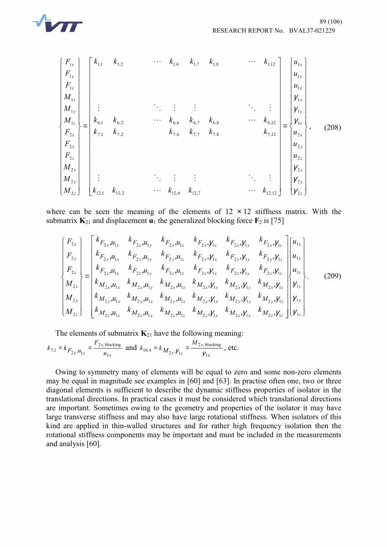
89 (106)RESEARCH REPORT No. BVAL37-021229
��������
�
��������
�
�
��������
�
��������
�
�
=
�����������������
�����������������
�
=
��������
�
��������
�
�
��������
�
��������
�
�
z
y
x
z
y
x
z
y
x
z
y
x
z
y
x
z
y
x
z
y
x
z
y
x
uuu
uuu
kkkkk
kkkkkkkkkkkk
kkkkkk
MMMFFFMMMFFF
2
2
2
2
2
2
1
1
1
1
1
1
12,127,126,122,121,12
12,78,77,76,72,71,7
12,68,67,66,62,61,6
12,18,17,16,12,11,1
2
2
2
2
2
2
1
1
1
1
1
1
γγγ
γγγ
��
������
��
������
��
, (208)
where can be seen the meaning of the elements of 12 × 12 stiffness matrix. With thesubmatrix K21 and displacement u1 the generalized blocking force F2 is [75]
����
�
����
�
�
����
�
����
�
�
����������
����������
�
=
����
�
����
�
�
����
�
����
�
�
z
y
x
z
y
x
zzyzxzzzyzxz
zyyyxyzyyyxy
zxyxxxzxyxxx
zzyzxzzzyzxz
zyyyxyzyyyxy
zxyxxxzxyxxx
z
y
x
z
y
x
u
u
u
kkkukukuk
kkkukukuk
kkkukukuk
kkkukukuk
kkkukukuk
kkkukukuk
M
M
M
F
F
F
MMMMMM
MMMMMM
MMMMMM
FFFFFF
FFFFFF
FFFFFF
1
1
1
1
1
1
121212121212
121212121212
121212121212
121212121212
121212121212
121212121212
2
2
2
2
2
2
,,,,,,
,,,,,,
,,,,,,
,,,,,,
,,,,,,
,,,,,,
γ
γ
γ
γγγ
γγγ
γγγ
γγγ
γγγ
γγγ
. (209)
The elements of submatrix K21 have the following meaning:
x
x
xx uF
uFkk1
blocking,2
1,21,7 == and 1x
blocking,2
1,24,10 γγx
xx
MMkk == , etc.
Owing to symmetry many of elements will be equal to zero and some non-zero elementsmay be equal in magnitude see examples in [60] and [63]. In practise often one, two or threediagonal elements is sufficient to describe the dynamic stiffness properties of isolator in thetranslational directions. In practical cases it must be considered which translational directionsare important. Sometimes owing to the geometry and properties of the isolator it may havelarge transverse stiffness and may also have large rotational stiffness. When isolators of thiskind are applied in thin-walled structures and for rather high frequency isolation then therotational stiffness components may be important and must be included in the measurementsand analysis [60].

90 (106)RESEARCH REPORT No. BVAL37-021229
13.2 Determination of power transmitted via vibrationisolator
13.2.1 Direct method
In the direct method the time averaged vibrational power which is transmitted through avibration isolator is determined by measuring the force and velocity directly ([19], [64], [65],and [74]) (see Figure 56). In the direct measurement method at each contact point one mustmeasure the force and vibration velocity in each excitation direction. In practise this is notalways possible because the force transducer cannot be installed in series with the isolator.For example following reasons can prevent installation of force transducer: there is not roomenough, the machine cannot be lifted because its shaft alignment cannot be changed, themeasurement must be made in-situ, force transducer is not mechanically durable, attachmentis not possible or its mass distorts the measurement results.
� � � � � � � $ � �3 � � � � $ � � � � & � �
� � �
Figure 56. Determination of structure-borne sound power transmission through an isolator. a)Direct method, and b) indirect method. Vibrational energy flows in the direction of thehatched arrow [64].
13.2.2 Indirect method
Structure-borne sound power transmission through an isolator can be determined indirectlyusing cross-spectral methods [61], [62], [63], and [64]. In this method the force is notmeasured directly. It is determined indirectly using the transfer stiffness of the isolator and thedisplacement of the upper surface of the isolator (see Figure 56). For these reasons the methodis often applicable if the measurements are to be made in-situ provided that there is enoughspace for the mounting of transducers.
Let us consider a vibration isolator under unidirectional excitation at the input point 1 andthat the output point 2 is blocked, e.g., its displacement is zero. The force exerted by theisolator on the receiving structure is obtained from Eqs. (197) and (200) as
1r
2,21,21
r
2,2
1,222,211,22 )1(
1u
kk
ku
kk
kukukF −≈
+=+= ,
(210)

91 (106)RESEARCH REPORT No. BVAL37-021229
where 1,2k is the blocked transfer stiffness over the isolator, i.e. it denotes the ratio betweenthe force on the blocked side and the displacement on the driven side, 2,2k is the driving-pointstiffness when the isolator is blocked at the opposite side, 1u is the vibration displacement atthe input point 1 and 2u is the vibration displacement at the output point 2. Theapproximation is valid within 10 % when r2,2 1,0 kk ⋅< [60].
The time average of structure-borne sound power transmitted t
P to the structure in onecontact point is obtained as time average of the product between the exciting force and theresulting velocity. This can be calculated from equation (e.g. [63], [31])
[ ] �∞
==⋅=0 222222 )(Re)0()()( dffGRtvtFEP vFvFt
, (211)
where [ ]E denotes the expected value of the expression inside the brackets, )0(22vFR is the
cross-correlation function between the force F2(t) and velocity v2(t) signals as a function ofthe delay time 0=τ , and )(
22fG vF is the one sided cross spectral density function between
the force F2(f) and velocity v2(f) signals. When the force and velocity are determined using themeasured acceleration signals then Eq. (211) can be written as
[ ]��∞ ∗
∗
∗∗∞
≈���
�
���
�−=
0 211,2321
2,21,20 3 )(ˆIm)()ˆ
ˆ1(ˆIm dffGkdffG
k
kkP aaaa
rt ωω
, (212)
where )(21
fG aa is the one sided cross spectral density between the measured acceleration
signals a1(f) at the input and a2(f) at the output of the vibration isolator, 1,2k is the blocked
transfer stiffness of the isolator, 2,2k is the blocked driving-point stiffness of the isolator, rkis the driving-point stiffness of the receiving structure, ( )⋅ denotes Fourier transform, andsymbol ( )∗⋅ denotes complex conjugate. Usually the driving-point stiffness of the receivingstructure is much larger than the driving-point stiffness of a soft vibration isolator and thenthe approximations of Eq. (210) and (212) can be used. From Eq. (212) one can see that forthe determination of the structure-borne sound power transmission through a vibrationisolator the dynamic blocked transfer stiffness of the isolator is needed. The dynamic blockedtransfer stiffness can be determined using test rigs constructed for this purpose (e.g. [63], [64],[67], [68], [71], [72]). In addition the acceleration signal a1 on the excited side and theacceleration signal a2 on the output side of the isolator are measured using standardizedmethod [73]. With these quantities the approximate time average of the transmitted power canbe determined. In case that there are many isolators one can assume that the powertransmitted through one isolator is independent on the power transmitted through otherisolators. Then the approximate time average of the total power through N isolators isobtained as a sum
�=
=N
1 tot,
itit PP , (213)
92 (106)RESEARCH REPORT No. BVAL37-021229
where tiP is the time average of the power transmitted through isolator i.
13.2.3 Generalization of the indirect method
The characterization of the dynamic properties of vibration isolators can be generalized toinclude all directions of translational and rotational vibrations using generalized force anddisplacement at contact points (e.g. [63], [64]). If forces and moments can be characterized bysix orthogonal components including three translations and three rotations, then the isolatormay be described as a 12-port [63]. Using the generalized force defined in Eq. (205) and(206) and the generalized displacement redefined in Eq. (203) and (204) the Fouriertransformed equilibrium equations can be written
2121111ˆˆˆˆˆ uKuKF += , (214)
and
2221212ˆˆˆˆˆ uKuKF += , (215)
where 11K and 22K are the Fourier transformed blocked dynamic driving-point 6 x 6
stiffness matrices and 12K and 21K are the Fourier transformed blocked dynamic transfer 6 x
6 stiffness matrices [64]. From reciprocity it follows that T2112
ˆˆ KK = , T1111
ˆˆ KK = andT2222
ˆˆ KK = , with T denoting a transpose [64]. In vibration isolation the objective is to get alarge source-receiving structure path stiffness mismatch. Usually driving-point stiffness of thereceiving structure is much large than the isolator stiffness, then [63]
1212ˆˆˆ uKF ≈ . (216)
This approximation reduces the number of needed stiffness elements for a single isolator to6636 ×= . Further reductions can be obtained due to isolator shape symmetries (see [60],
[63], [75]). The metal plates at the ends of an isolator can be considered to be integrated to thereceiving structure, because the stiffness mismatch is at the rubber-plate interface [64]. Incases where the approximation of Eq. (216) can not be used Eq. (215) still applies resulting toelement number 666672 ×+×= for the accurate force estimation at the receiving structure[64].
With cross-spectral techniques the power transmission through vibration isolator toreceiving structure in different degrees of freedom can be determined indirectly [64], [66].The total power transmitted is obtained as a sum of powers in different degrees of freedom. Inthe measurement technique one needs to measure the vibration velocities of resilientlymounted machinery. This can be made using standardized methods [73]. Also the neededdynamic transfer stiffnesses of isolators can be measured using standardized methodsdescribed in [60], [74], [75].
Amunarriz has studied the power transmission over a cylindrical rubber isolator [66]. Thediameter of the isolator was 100 mm, height 54 mm and hardness 40° IRH (InternationalRubber Hardness). In the frequency range 20 Hz - 1 kHz 97 % was transmitted bytranslational degrees of freedom, 2,1 % by cross couplings and 0,9 % by rotational degrees.At low frequencies in the frequency range 20 Hz - 500 Hz the share of translational degreeswas 96 % and that of rotational degrees 4 %. At high frequencies in the frequency range

93 (106)RESEARCH REPORT No. BVAL37-021229
500 Hz - 1 kHz the share of translational degrees decreases to 91 % and there is an increase inthe contribution of rotational degrees reaching 5 % and cross couplings reaching 4 % [66].These approximate results can give guidance when considering the effect of rotational andcross coupling components in the power transmission through vibration isolators inengineering applications.
14 Research and test facilities of vibrationisolators
14.1.1 Research and facilities at KTH, Sweden
In Sweden at KTH, The Royal Institute of Technology, active research and testing has beendone for years in The Marcus Wallenberg Laboratory for Sound and Vibration Research(MWL) leaded by professor Anders Nilsson [64], [65], [66].
Let us take an example of the research work done in this laboratory. Leif Kari hasmeasured in six degrees of freedom up to 1 000 Hz the blocked dynamic transfer stiffness of acylindrical rubber vibration isolator under four different static preloads [64]. He has alsodeveloped models and made theoretical calculations of transfer stiffness of rubber mounts. Heapplied correlation technique and stepped sine excitation to improve the signal to noise ratio.Indirect test method is used in the KTH test rig (Figure 57). Kari has studied a vulcanizednatural rubber isolator. Its length was 50 mm, radius 50 mm, and hardness 40° IRH(International Rubber Hardness). The allowed continuous static load was limited to 3 000 N.He measured the axial static force due to axial deformation in the domain 0 - 12 mm in stepsof approximately 1 mm. The measured axial dynamic stiffness in the frequency range 50 - 1 000 Hz under different preloads is presented in Figure 59 and Figure 60. The stiffnessmagnitude curve in Figure 59 is plateau like in the low frequencies up to about 400 Hz.Thereafter the curve rises to a peak at 500 Hz, drops to a trough, rises to a second peak and soon. Taking into account the magnitude curve with the phase curve, the three peaks occurlikely at anti resonance and the first and the third troughs are likely connected to resonances[64].

94 (106)RESEARCH REPORT No. BVAL37-021229
Figure 57. Schematic presentation of the test rig of vibration isolators at KTH [65]. It is basedon indirect method. The parts are: A isolator under test, B force distribution plate, C blockingmass, D piezoelectric accelerometers, E strain gage, F electrodynamic vibration generators, Gupper auxiliary isolator, H lower auxiliary isolator, I heavy and rigid frame, J strong columns,and K crosshead.
Figure 58. Measured axial compression force versus corresponding displacement. Test objectis the rubber vibration isolator [64].

95 (106)RESEARCH REPORT No. BVAL37-021229
Figure 59. Measured magnitude of transfer stiffness. Test object is the rubber vibrationisolator. 0 N (solid thin), 1 600 N (dashed), 2 100 N (dotted) and 3 350 N preload (dash-dotted) [64].
Figure 60. Measured unwrapped phase of transfer stiffness. Test object is the rubber vibrationisolator. 0 N (solid thin), 1 600 N (dashed), 2 100 N (dotted) and 3 350 N (dash-dotted) [64].

96 (106)RESEARCH REPORT No. BVAL37-021229
14.1.2 Research and facilities at AMRL, Australia
In Australia testing of vibration isolators is made in The Aeronautical and Maritime ResearchLaboratory (AMRL). This laboratory belongs to Defence Science and TechnologyOrganization (DSTO). There Dickens and Norwood propose a two-mass method to determinethe four-pole parameters of a uni-directional asymmetrical vibration isolator [67]. They havedeveloped and tested a test rig shown in Figure 61.
Figure 61. Schematic diagram of vibration isolator test rig [67].
The test rig employs the floating mass method and direct force measurement and it mayalso employ the two-mass method. Vibration isolators operated in lateral and transverseorientations may also be tested with this test facility. Vibration isolator is mounted betweentwo large masses. An electro-dynamic shaker via the excitation mass applies the dynamicload. The floating mass provides a reaction force to the output force of the vibration isolator.Air bags are used to produce easily adjustable static load. They also give good vibrationisolation between the mass and the supporting structure. The seismic mass of 22 tons withdimensions 3 m × 3 m × 1 m is made of reinforced concrete. It is supported on four air bags.The mounted natural frequency of this test facility is approximately 1,2 Hz. The upper framesupports the shaker. The lower frame provides the reaction forces for the upper static loading

97 (106)RESEARCH REPORT No. BVAL37-021229
air bags. The two frames are used to reduce the coupling between the preloading structure andthe shaker. The vibration due to flanking transmission is 90 dB smaller than the vibrationlevel due to direct transmission. The vibration velocities at input and output of the vibrationisolator are measured with accelerometers attached to the excitation and floating masses. Thedynamic force applied by the excitation mass to the vibration isolator is measured directlywith a force measuring assembly consisting of eight force transducers. The test facility isconstructed to measure dynamic stiffness in the range of N/m 102101 75 ×−× with preloadsvarying from 1,5 to 30 kN and over a frequency range from 10 Hz to 2 000 Hz [68].
With the test facility it is possible to determine the four-pole parameters of an uni-directional or bi-directional, and asymmetrical or symmetrical vibration isolator under staticload. Generally vibration isolators incorporating some form of active control are examples ofuni-directional vibration isolators [68].
The method proposed by Dickens and Norwood to dynamically characterize vibrationisolators with four-pole parameters has three advantages [67]. Firstly, the characterization isindependent of the method. Traditionally the transmissibility of a vibration isolator isdetermined by attaching a mass on the isolator, which in turn is supported on a rigidfoundation. Then a shaker excites the mass and the output of the vibration isolator isconsidered to be blocked. The transmissibility is determined as the ratio of the output force ofthe vibration isolator to the input force excerted to the mass. So it depends on the supportedmass, and is not independent on the test arrangement. Secondly, at high frequencies evidentmass effects of the vibration isolator are taken into account. In traditional methods thedistribution of mass and stiffness of the vibration isolator are not included. So the masslessspring model fails to predict the existence of the longitudinal standing waves which reducethe performance of real vibration isolators. Thirdly, the four-pole parameters of a complicatedmechanical system can be computed from the four-pole parameters of its components.
The traditional methods for the determination of four-pole parameters of a vibrationisolator under static preload use blocked test configuration. Because asymmetrical vibrationisolators require additional information which is obtained by reversing the vibration isolatorin the test rig meaning that its input and output sides are interchanged. This procedure isinapplicable for uni-directional vibration isolators as for active vibration isolators [67].
14.1.3 Research and facilities at TNO TPD, The Netherlands
The TNO Institute of Applied Physics - Technisch Physische Dienst (TNO TPD) has beencarrying out an active and extensive research on resilient elements since 1975. In this contextvarious test facilities have been developed for measuring the sound transfer and the dynamicstiffness of resilient components in the six degrees of freedom under normal operationalconditions, such as static preload and internal pressure [71], [72]. In the test rigs the realcomponent properties can be measured for multi-directional excitation under operationalstatic load. In a test rig (Figure 62 and Figure 63)

98 (106)RESEARCH REPORT No. BVAL37-021229
Figure 62. (a) Schematic diagram of the measurement apparatus (not to scale), shoving maindimensions. (b) Equivalent mass-spring system [69].
Figure 63. Test facility with a flexible shaft under test in the axial excitation mode (torsionalpreload with two hydraulic cylinders) [71].
the vibration isolator under test is assembled between two masses. The upper mass simulatesthe machine side and acts as an excitation mass. The lower mass is used to determine the so-called blocked forces, which a flexible element exerts on high impedance seating. The seatingis the local attachment point on the receiving substructure to which the "lower" end of theisolator is attached [19]. The frequency range of interest determines the sizes and dimensionsof these masses. In the measurement range over the natural frequency of the system the soundtransfer functions and the dynamic stiffnesses can be determined. Changing the direction ofexcitation this determination can be made in all other degrees of freedom. Flexible saftcouplings up to 1 m diameter and 75 kNm torsional preload can be tested in the largest testrig. The torsional preload is obtained with pneumatic or hydraulic auxiliaries.

99 (106)RESEARCH REPORT No. BVAL37-021229
Resilient mountings can be measured in a hydraulic pressure test bench. The mounting isassembled between two masses, which vibrate as free, rigid bodies in the frequency rangeconsidered. The mounting and the masses are decoupled from the frame with auxiliary softmountings. These mountings provide support and static preload. The electrodynamic shakerconnected to the excitation mass produces the excitation. The measurements are made usingaccelerometers. Selection of masses and auxiliary mountings provides a useful measurementfrequency range from 20 Hz to 2 000 Hz [71], [72]. The dimensions of the masses can bechanged to obtain the upper measurement limit of 4 kHz [70]. In the largest test rig thepreload can be 100 tons. The measurements are made according to standard ISO 10846, parts1-5 [72].
Figure 64. Test facility with rubber mounting under test in the vertical excitation mode [71].Bellows and flexible hoses can be tested in similar test rigs as is used for mountings andcouplings (see Figure 65). The measurements are made under real pressure conditions insidethe elements.
Figure 65. Test facility for flexible hoses and bellows. An auxiliary system (mass and house)has been connected to eliminate the effects of fluid-borne sound transmission to the blockingmass [71].

100 (106)RESEARCH REPORT No. BVAL37-021229
14.1.4 Research and facilities at HUT and VTT, Finland
A test facility (Figure 66) for the measurement of dynamic properties of vibration isolatorsunder preload according to the direct method of ISO 10846 was constructed by Laboratory forMechanics of Materials and VTT Industrial Systems [76], [79]. This laboratory belongs to theDepartment of Mechanical Engineering at Helsinki University of Technology. It is located atEspoo city. The research of dynamic properties of vibration isolators done in co-operationwith participants from both organizations is one subprogram of the technology programControl of Vibration and Sound VÄRE (1999-2002). This programme is funded by NationalTechnology Agency (Tekes) of Finland.
Upper mass
Lower mass
Loading cylinder
Accelerometer
Accelerometer
Preload tarnsducer
Vibrationisolator
Force distributiondevices
Force transducer
Upper and lower mass
• breadth 750 mm• height 297 mm• depth 297 mm• mass 254 kg
Steel cylinders• diameter 100 mm• length 1500 mm• mass 92 kg
Bolt M24 (24 pieces)• length 240 mm• mass 1,1 kg
Figure 66. Test rig for the measurement of dynamic properties of vibration isolators accordingto the direct method of ISO 10846 at Helsinki University of Technology, Department ofMechanical Engineering in the Laboratory for Mechanics of Materials in Espoo city.
Two steel cylinders form the frame of the test rig. Between them is attached two adjustablemasses. The total mass of the frame structure is 720 kg. Some modifications were made to theoriginal test rig [76], and now the test rig is planned to achieve the following operatingparameters [79]:- The requirements of ISO 10846 are fulfilled in the application area- Displacement amplitude of the excitation from 0,1 to 2 mm- Static preload up to 4 kN- Frequency range up to 240 Hz, but depends on preload and amplitude- Vibration isolators with diameters up to 200 mm can be attached. The length of a vibration
isolator is not fixed, because the location of the upper mass can be adjusted.

101 (106)RESEARCH REPORT No. BVAL37-021229
Some research has been done on wire rope vibration isolators using the indirect method ofISO 10846, part 3 [77], [78]. This wire rope research belongs also to VÄRE technologyprogramme. The test facilities of VTT Industrial Systems in the research area IntelligentProducts and Services include the Ling Dynamic Systems 455 series vibrator with mass81,6 kg. It may produce a maximum sinusoidal force of 489 N when external cooling fan isused. When only natural cooling is used then only a force of 177 N is available. The availablefrequency range is from 10 Hz to 7 500 Hz. The maximum displacement amplitude of theshaker table is 9,5 mm and the maximum velocity 2,5 m/s. Maximum acceleration of baretable is 117 g. Effective mass of the moving system is 0,43 kg. A rated force, random rms flatspectrum 20 - 2 000 Hz, of 283 N can be achieved with payload equal to or greater thanarmature moving mass of 0,43 kg.
VTT Industrial Systems has also mechanical test facilities at Espoo includingelectrodynamical vibrators. Their main characteristics are maximum force 35,6 kN, frequencyrange 5 … 2 000 Hz, maximum acceleration 1 100 m/s2, maximum velocity 1,8 m/s, andmaximum amplitude 50 mm.
15 ConclusionsTypically a machine is mounted on a flexible foundation. These installations are to bedesigned for minimum vibration and sound radiation. In these analysis vibrational powertransmission analysis, both analytical and experimental, is beneficial when the transmissionpaths from machine are assessed. The power transmitted from a machine to its foundation isnot only dependent on the source strength of the machine, but it is also dependent both on thesource and receiver dynamical characteristics. That is why a designer needs to know thereceiver and source mobilities with the free velocity of the machine to be installed. If themachine is mounted via a set of vibration isolators, then their dynamic transfer stiffness isneeded. This can be obtained using standardized measurements. Depending on the applicationa unidirectional model may be sufficient, otherwise the dynamic characteristics of isolatorsneeds to be known in other relevant translational and rotational degrees of freedom.
Experimentally the power transmission can be estimated in-situ. This method is based onthe structural power calibration of the receiving structure, which is made before the source isinstalled. An approximate transmission estimate can be obtained with the source alreadyinstalled, provided that either the source or receive mobility is available at the contact points.
There is still a need for continued research work towards internationally accepted methodsfor the characterization of structure-borne sound sources and for predicting the transmissionof structure-borne sound power into source foundations and receiving structures. However,progress has been made in recent years in this respect. Engineers being unable to predictvibration and sound levels of real structures all but at very low frequencies using numericalpackages like FEM or BEM are seeking other solutions like energy-related methods. In thesemethods the structure-borne sound power can be used in the prediction of resulting vibrationand sound levels.

102 (106)RESEARCH REPORT No. BVAL37-021229
References[1] ISO/TR 11688-1. Acoustics - Recommended practice for the design of low-noise
machinery and equipment - Part 1: Planning. Geneva: International Organization forStandardization, 1995. 36 pp.
[2] ISO/TR 11688-2. Acoustics - Recommended practice for the design of low-noisemachinery and equipment - Part 2: Introduction to the physics of low-noise design.Geneva: International Organization for Standardization, 1998. 46 pp.
[3] ISO/TR 11690-3. Acoustics - Recommended practice for the design of low-noiseworkplaces containing machinery - Part 3: Sound propagation and noise prediction inworkrooms. Geneva: International Organization for Standardization, 1997. 36 pp.
[4] Koopmann, G. H. & Fahnline, J. B. Designing quiet structures. A sound powerminimization approach. San Diego. Academic Press, 1997. 244 pp.
[5] Pierce. A. D. Acoustics. An introduction to its physical principles and applications. 2nd.ed. New York: The Acoustical Society of America, 1991. 678 pp.
[6] Carlsson, U. Mechanical mobility: A tool for the analysis of vibrations in mechanicalstructures (Doctoral thesis). Stockholm: Technical acoustics, Department of VehicleEngineering, Royal Institute of Technology. Marcus Wallenberg Institute for Soundand Vibration Research, 1993. 333 pp. (TRITA-FKT Report 9331)
[7] Fahy, F. Manfred Heckl memorial lecture: The role of experimentation invibroacoustics. In: Proc. of the third European Conference on Noise Control, EURO-NOISE 98. Munich, Germany. Oldenburg, Germany: German Acoustical Society(DEGA), 1998. Pp. 3-14.
[8] Lyon, R. H. & DeJong, R. G. Theory and application of statistical energy analysis. 2nd.ed. Boston, Massachusetts, USA: Butterworth-Heinemann. 1995. 277 pp.
[9] Wolde, T. ten & Gadefelt, G. R. Development of standard measurement methods forstructureborne sound emission. Noise Control Engineering Journal, 1987.Vol. 28, no. 1, pp. 5-14.
[10] Mondot, J. M. & Pettersson, B. Characterization of structure-borne sound sources: Thesource descriptor and the coupling function. Journal of Sound and Vibration, 1987. Vol.114, no. 3, pp. 507-518.
[11] Koh, Y. K. & White, R. G. Analysis and control of vibrational power transmission tomachinery supporting structures subjected to a multi-excitation system, Part I: Drivingpoint mobility matrix of beams and rectangular plates. Journal of Sound and Vibration,1996. Vol. 196, no. 4, pp. 469-493.
[12] Koh, Y. K. & White, R. G. Analysis and control of vibrational power transmission tomachinery supporting structures subjected to a multi-excitation system, Part II:Vibrational power analysis and control schemes. Journal of Sound and Vibration, 1996.Vol. 196, no. 4, pp. 495-508.
[13] Koh, Y. K. & White, R. G. Analysis and control of vibrational power transmission tomachinery supporting structures subjected to a multi-excitation system, Part III:Vibrational power cancellation and control experiments. Journal of Sound andVibration, 1996. Vol. 196, no. 4, pp. 509-522.
[14] Fulford, R. A. & Gibbs, B. M. Structure-borne sound power and source characterisationin multi-point-connected systems, Part 1: Case studies for assumed force distributions.Journal of Sound and Vibration, 1997. Vol. 204, no. 4, pp. 659-677.
[15] Fulford, R. A. & Gibbs, B. M. Structure-borne sound power and source characterizationin multi-point-connected systems, Part 2: About mobility functions and three velocities.Journal of Sound and Vibration, 1999. Vol. 220, no. 2, pp. 203-224.

103 (106)RESEARCH REPORT No. BVAL37-021229
[16] Fulford, R. A. & Gibbs, B. M. Structure-borne sound power and source characterizationin multi-point-connected systems, Part 3: Force ratio estimates. Journal of Sound andVibration, 1999. Vol. 225, no. 2, pp. 239-282.
[17] Grice, R. M. & Pinnington, R. J. A method for the vibration analysis of built-upstructures, Part I: Introduction and analytical analysis of the plate-stiffened beam.Journal of Sound and Vibration, 2000. Vol. 230, no. 4, pp. 825-849.
[18] Grice, R. M. & Pinnington, R. J. A method for the vibration analysis of built-upstructures, Part II: Analysis of the plate-stiffened beam using a combination of finiteelement analysis and analytical impedances. Journal of Sound and Vibration, 2000. Vol.230, no. 4, pp. 851-875.
[19] White, R. G. Power transmission measurement and control in structures. In: Pavic, G.(ed.) Novem 2000 proceedings. Lyon, France, 31 August-2 September, 2000. Lyon:Laboratoire Vibrations Acoustique, INSA de Lyon, 2000. 11 pp.
[20] Fahy, F. Foundations of Engineering Acoustics. San Diego. Academic Press, 2001. 443pp.
[21] ISO 7626-1. 1986. Vibration and shock - Experimental determination of mechanicalmobility - Part 1: Basic definitions and trasducers. Geneva: International Organizationfor Standardization. 23 pp.
[22] ISO 2041. 1990. Vibration and shock - Vocabylary. Geneva: International Organizationfor Standardization. 59 pp.
[23] Cremer, L., Heckl, M. & Ungar, E. E. (transl.). Structure-borne sound. 2nd. ed. Berlin:Springer-Verlag, 1988. 573 pp.
[24] Cremer, L., Heckl, M. & Ungar, E. E. (transl.). Structure-borne sound. Berlin: Springer-Verlag, 1973. 528 pp.
[25] Ten Wolde, T., Verheij, J. W. & Steenhoek, H. F. Reciprocity method for themeasurement of mechano-acoustical transfer functions. Journal of Sound and Vibration,1975. Vol. 42, no. 1, pp. 49-55.
[26] Fahy, F. Sound and Structural Vibration. Radiation, Transmission and Response.London: Academic Press, 1985. 309 pp.
[27] Goyder, H. G. D. & White, R. G. Vibrational power flow from machines into built-upstructures, Part I: Introduction and approximate analyses of beam and plate-likefoundations. Journal of Sound and Vibration, 1980. Vol. 68, no. 1, pp. 59-75.
[28] Goyder, H. G. D. & White, R. G. Vibrational power flow from machines into built-upstructures, Part II: Wave propagation and power flow in beam-stiffened plates. Journalof Sound and Vibration, 1980. Vol. 68, no. 1, pp. 77-96.
[29] Goyder, H. G. D. & White, R. G. Vibrational power flow from machines into built-upstructures, Part III: Power flow through isolation systems. Journal of Sound andVibration, 1980. Vol. 68, no. 1, pp. 97-117.
[30] O'Hara, G. J. Mechanical impedance and mobility concepts. The Journal of theAcoustical Society of America, 1967. Vol. 41, no. 5, pp. 1180-1184.
[31] Nilsson, A. C. Vibroacoustics, Part I. Stockholm: KTH, Department of VehicleEngineering, MWL The Marcus Wallenberg Laboratory for Sound and VibrationResearch, 2000, 208 pp. (Royal Institute of Technology - TRITA-FKT 2000:14.)
[32] Nilsson, A. C. Vibroacoustics, Part II. Stockholm: KTH, Department of VehicleEngineering, MWL The Marcus Wallenberg Laboratory for Sound and VibrationResearch, 2000, 263 pp. (Royal Institute of Technology - TRITA-FKT 2000:15.)
[33] Rubin, S. Mechanical immittance- and transmission-matrix concepts. The Journal of theAcoustical Society of America, 1967. Vol. 41, no. 5, pp. 1171-1179.
[34] Molloy, C. T. Use of four-pole parameters in vibration calculations. The Journal of theAcoustical Society of America, 1957. Vol. 29, no. 7, pp. 842-853.
104 (106)RESEARCH REPORT No. BVAL37-021229
[35] Snowdon, J. C. Mechanical four-pole parameters and their application. Journal of Soundand Vibration, 1971. Vol. 15, no. 3, pp. 307-323.
[36] Hixson, E. L. Mechanical impedance. In: Harris, C. M. (ed.). Shock and vibrationhandbook. 3rd ed. New York: McGraw-Hill, 1988. Chapter 10.
[37] Petersson, B. & Plunt, J. On effective mobilities in the prediction of structure-bornesound transmission between a source structure and a receiving structure, Part I:Theoretical background and basic experimental studies. Journal of Sound and Vibration,1982. Vol. 82, no. 4, pp. 517 - 529.
[38] Petersson, B. & Plunt, J. On effective mobilities in the prediction of structure-bornesound transmission between a source structure and a receiving structure, Part II:Procedures for the estimation of mobilities. Journal of Sound and Vibration, 1982. Vol.82, no. 4, pp. 531 - 540.
[39] Petersson, B. & Plunt, J. Stomljudstransmission från maskiner till undederlag.Göteborg: Avdelning för Byggnadsakustik, Chalmers Tekniska Högskola, 1979. 51 pp.+ app. 17 pp. (Rapport 79-13)
[40] Petersson, B. A. T. & Gibbs, B. M. Towards a structure-borne sound sourcecharacterization. Applied Acoustics, 2000. Vol. 61, no. 3, pp. 325-343.
[41] Beranek, L. L. (ed.). Noise and Vibration Control. Rev. ed. Cambridge, MA, USA:Institute of Noise Control Engineering, 1988. 672 pp.
[42] ISO 7626-2. 1990. Vibration and shock - Experimental determination of mechanicalmobility - Part 2: Measurements using single-point translation excitation with anattached vibration exciter. Geneva: International Organization for Standardization. 21pp.
[43] Petersson, B. A. T. & Gibbs, B. M. Use of the source descriptor concept in studies ofmulti-point and multi-directional vibrational sources. Journal of Sound and Vibration,1993. Vol. 168, no. 1, pp. 157-176.
[44] Petersson, B. A. T. & Plunt, J. Structure-borne sound transmission from machinery tofoundations. Gothenburg, Sweden: Department of Building Acoustics, ChalmersUniversity of Technology, 1980. 120 pp. (Report 80-19)
[45] Skudrzyk, E. J. The mean-value method of predicting the dynamic response of complexvibrators. The Journal of the Acoustical Society of America, 1980. Vol. 67, no. 4, pp.1105-1135.
[46] Skudrzyk, E. J. Understanding the dynamic behaviour of complex vibrators. Acustica,1987. Vol. 64, no. 3, pp. 123-147.
[47] Gibbs, B. M., Petersson, B. A. T. & Qiu, S. The characterization of structure-borneemission of building services machinery using the source descriptor concept. NoiseControl Engineering Journal, 1991. Vol. 37, no. 2, pp. 53-61.
[48] Ewins, D. J. State-of-the-art assessment of mobility measurements – A summary ofEuropean results. The Shock and Vibration Bulletin, 1981. Bulletin 51, Part 1, pp. 15-35.
[49] Ewins, D. J. State-of-the-art assessment of mobility measurement techniques (SAMM) -– Summary of results. Journal of the Society of Environmental Engineers, 1981. Vol.20, no. 1, pp. 3-13.
[50] ISO 7626-5. 1994. Vibration and shock - Experimental determination of mechanicalmobility - Part 5: Measurements using impact excitation with an exciter which is notattached to the structure. Geneva: International Organization for Standardization. 22 pp.
[51] Ohlrich, M. In-situ estimation of structural power transmission from machinery sourceinstallations. In: Jacobsen, F. (ed.) Proceedings of the Sixth International Congress onSound and Vibration. Copenhagen, Denmark, 5-8 July, 1999. Lungby: Department ofAcoustic Technology, Technical University of Denmark, 1999. Vol. 5, pp. 2149-2160.

105 (106)RESEARCH REPORT No. BVAL37-021229
[52] Ohlrich, M. A simple structural power method for determining the vibratory strength ofmachinery sources. In: Proceedings of Euro-Noise 98. München, Germany, 4-7October, 1998. Vol. 1, pp. 383-388.
[53] Ohlrich, M. Terminal source power for predicting structure-borne sound transmissionfrom a main gearbox to a helicopter fuselage. In: Bernhard, R. J. & Bolton, J. S. (ed.).Proceedings of Inter-Noise 95. Newport Beach, California, USA, 10-12 July, 1995. Vol.1, pp. 555-558.
[54] Ohlrich, M. & Larsen, C. Surface and terminal source power for characterization ofvibration sources at audible frequencies. In: Kuwano, S. (ed.). Proceedings of Inter-Noise 94. Yokohama, Japan, 29-31 August, 1994. Vol. 1, pp. 633-636.
[55] Moorhouse, A. T. & Gibbs, B. M. Prediction of the structure-borne noise emission ofmachines: Development of a methodology. Journal of Sound and Vibration, 1993. Vol.167, no. 2, pp. 223-237.
[56] Moorhouse, A. T. & Gibbs, B. M. Structure-borne sound power emission fromresiliently mounted fans: Case studies and diagnosis. Journal of Sound and Vibration,1995. Vol. 186, no. 5, pp. 781-803.
[57] Ohlrich, M. The use of surface power for characterisation of structure-borne soundsources of low modal density. In: Hill, F. A. & Lawrence, R. (ed.). Proceedings of Inter-Noise 96. Liverpool, United Kingdom, July 30 - August 02, 1996. Book 3, pp. 1313-1318.
[58] Ohlrich, M. & Crone, A. An equivalent force description of gearbox sources applied inprediction of structural vibration in wind turbines. In: Proceedings of Inter-Noise 88.Pp. 479-484.
[59] Laugesen, S. & Ohlrich, M. The vibrational source strength descriptor using powerinput from equivalent forces: a simulation study. Acta Acoustica, 1994. Vol., no. 2, pp.449-459.
[60] ISO 10846-1. Acoustics and vibration - Laboratory measurement of vibro-acoustictransfer properties of resilient elements - Part 1: Principles and guidelines. Geneva: theInternational Organization for Standardization, 1997. 20 pp.
[61] Pinnington, R. J. & White, R. G. Power flow through machine isolators to resonant andnon-resonant beams. Journal of Sound and Vibration, 1981. Vol. 75, no. 24, pp. 179-197.
[62] Pinnington, R. J. Vibrational power transmission to a seating of a vibration isolatedmotor. Journal of Sound and Vibration, 1987. Vol. 118, no. 1, pp. 123-139.
[63] Verheij, J. W. Multi-path sound transfer from resiliently mounted shipboard machinery(Doctoral thesis). Delft, The Netherlands: Technisch Physische Dienst TNO-TH(Institute of Applied Physics TNO-TH), 1982. 267 pp.
[64] Kari, L. Structure-borne sound properties of vibration isolatos (Doctoral thesis).Stockholm: Royal Institute of Technology, Department of Vehicle Engineering. TheMarcus Wallenberg Laboratory for Sound and Vibration Research, 1998. 26 pp. +appendices A-D. (TRITA-FKT Report 9802)
[65] Kari, L. Dynamic transfer stiffness measurements of vibration isolators in the audiblefrequency range. Noise Control Engineering Journal, 2001. Vol. 49, no. 2, pp. 88-102.
[66] Amunarriz, G. Indirect measurements of structure-borne sound energy flow throughvibration isolators (Master Thesis). Stockholm: Royal Institute of Technology,Department of Vehicle Engineering. The Marcus Wallenberg Laboratory for Sound andVibration Research, 1999. 57 pp. + appendices. 18 pp. (TRITA-FKT Report 9902)
[67] Dickens, J. D. & Norwood, C. J. Universal method to measure dynamic performance ofvibration isolators under static load. Journal of Sound and Vibration, 2001. Vol. 244,no. 4, pp. 685-696.

106 (106)RESEARCH REPORT No. BVAL37-021229
[68] Dickens, J. D. & Norwood, C. J. Design of a test facility for vibration isolatorcharacterisation. Acoustics Australia, 1997. Vol. 25, no. 1, pp. 23- 28.
[69] Thompson, D. J., van Vliet, W. J. & Verheij, J. W. Developments of the indirect methodfor measuring the high frequency dynamic stiffness of resilient elements. Journal ofSound and Vibration, 1998. Vol. 213, no. 1, pp. 169-188.
[70] Thompson, D. J. & Verheij, J. W. The dynamic behaviour of rail fasteners at highfrequencies. Applied Acoustics, 1997. Vol. 52, no. 1, pp. 1-17.
[71] Flexible components. Netherlands organization for applied scientific research TNO.TNO Institute of Applied Physics. Leaflet 8-89. 4 pp.
[72] Ship Acoustics. Testing quality and the acoustic properties of flexible elements. TNOTPD. Leaflet 112001/200. 2 pp.
[73] ISO 9611. Acoustics - Characterization of sources of structure-borne sound with respectto sound radiation from connected structures - Measurement of velocity at the contactpoints of machinery when resiliently mounted. Geneva: the International Organizationfor Standardization, 1996. 19 s.
[74] ISO 10846-2. Acoustics and vibration - Laboratory measurement of vibro-acoustictransfer properties of resilient elements - Part 2: Dynamic stiffness of elastic supportsfor translatory motion - Direct method. Geneva: The International Organization forStandardization, 1997. 18 s.
[75] ISO/FDIS 10846-3. Acoustics and vibration- Laboratory measurement of vibro-acoustictransfer properties of resilient elements - Part 3: Dynamic stiffness of resilient supportsfor translatory motion (Indirect method). Geneva: The International Organization forStandardization, 2002. 38 s.
[76] Rantala, J. Development of Testing Arrangement for Vibration Isolators Based on ISO10846 Standard. Espoo: Helsinki University of Technology. Department of MechanicalEngineering. Laboratory for Mechanics of Materials 2000. 19 pp. + app. 10 pp. (inFinnish)
[77] Linjama, J. & Juntunen, M. Estimation of dynamic properties of resilient mounts. In:Friswell, M. I., Mottershead, J. E. & Lees, A. W. (ed.). Proceedings of the SecondInternational Conference. Identification in Engineering systems. Swansea, UK, March29-31, 1999. Pp. 74 - 83.
[78] Juntunen, M. & Linjama, J. A test method for estimation of dynamic properties ofisolators. In: Güemes, J. A. (ed.). Proceedings of European COST F3 Conference onSYSTEM IDENTIFICATION & STRUCTURAL HEALTH MONITORING. Vol. 2.Madrid, Spain, June, 2000. Madrid: Universidad Politécnica de Madrid, Spain. Pp. 815 -829.
[79] Keinänen, J. Testing and modelling dynamic properties for vibration isolators. Espoo:Helsinki University of Technology, Department of Mechanical Engineering, Laboratoryfor Mechanics of Materials, 2002. 95 pp. + app. (Master of Science thesis)
[80] Moorhouse, A. T. On the characteristic power of structure-borne sound sources. Journalof Sound and Vibration, 2001. Vol. 248, no. 3, pp. 441-459.