virtual laboratory of remote sensing time series: visualization … · virtual laboratory of remote...

“main” — 2011/7/30 — 11:41 — page 57 — #1

Journal of Computational Interdisciplinary Sciences (2011) 2(1): 57-68© 2011 Pan-American Association of Computational Interdisciplinary SciencesPrinted version ISSN 1983-8409 / Online version ISSN 2177-8833http://epacis.org

Virtual laboratory of remote sensing time series:

visualization of MODIS EVI2 data set over South America

Ramon Morais de Freitas1, Egidio Arai1, Marcos Adami1, Arley Souza Ferreira1,Fernando Yuzo Sato1, Yosio Edemir Shimabukuro1, Reinaldo Roberto Rosa1,Liana Oighenstein Anderson1,2 and Bernardo Friedrich Theodor Rudorff1

Manuscript received on February 4, 2011 / accepted on March 24, 2011

ABSTRACT

Over the last ten years millions of gigabytes of MODIS (Moderate Resolution Imaging Spectroradiometer) data have been generated

which is forcing the remote sensing users community to a new paradigm in data processing for image analysis and visualization of

these time series. In this context this paper aims to present the development of a tool to integrate the 10 years time series of MODIS

images into a virtual globe to support LULC change studies. Initially the development of a tool for instantaneous visualization of remote

sensing time series within the concept of a virtual laboratory framework is described. The virtual laboratory is composed by a data set

with more than 500 million EVI2 (Enhanced Vegetation Index 2) time series derived from MODIS 16-day composite data. The EVI2

time series were filtered with sensor ancillary data and Daubechies (Db8) orthogonal Discrete Wavelets Transform.

Then EVI2 time series were integrated into the virtual globe using Google Maps and Google Visualization Application Programming

Interface functionalities. The Land Use Land Cover changes for forestry and agricultural applications are presented using the proposed

time series visualization tool.

The tool demonstrated to be useful for rapid LULC change analysis, at the pixel level, over large regions. Next steps are to further

develop the Virtual Laboratory of Remote Sensing Time Series Framework by extending this work for other geographical regions,

incorporating new computational algorithms, testing data from other sensors and updating the MODIS time series.

Keywords: MODIS, EVI2, wavelets transform, time series analysis, virtual globe, land use and land cover changes, forest, agriculture,

South America, instantaneous visualization.

1 INTRODUCTION

Over the last few decades, multi-temporal images of Earth obser-

vation satellites have turned into a paramount source of informa-

tion for monitoring the planet Earth, particularly to study the land

use and land cover changes (LULC) [1]. Such studies are gaining

more attention not only by scientists but also by policy makers

and media, since terrestrial ecosystems exert major influence on

climate change and climate variability [2].

Remote sensing sensors such as: the AVHRR (Advanced VeryHigh Resolution Radiometer) on board of the NOAA (NationalOceanic and Atmospheric Administration) satellites; the Vege-tation on board of the SPOT (Satellite Pour l’Observation de laTerre) satellites; and the MODIS (Moderate Resolution Imaging

Correspondence to: Ramon Morais de Freitas – E-mail: [email protected] Institute for Space Research – INPE, Sao Jose dos Campos, SP, Brazil.2University of Oxford, Environmental Change Institute – ECI, Oxford, UK.

“main” — 2011/7/30 — 11:41 — page 58 — #2

58 VIRTUAL LABORATORY OF REMOTE SENSING TIME SERIES

Spectroradiometer) on board of the Terra (EOS-AM1) and Aqua(EOS-PM1) satellites have been responsible for the constructionof long term time series dataset. All these sensors acquire im-ages on an almost daily basis which is an important characteristicfor optical sensors designed to observe LULC changes. For theMODIS sensor a significant advancement was achieved by im-proving both spatial and spectral resolutions. Furthermore, aninternational consortium of scientists has focused on providingvalidated MODIS data with high radiometric and geometric qual-ity, since the launch of the Terra satellite [3]. Over the last tenyears millions of gigabytes of MODIS data have been generatedwhich is forcing the remote sensing users community to a newparadigm in data processing for image analysis and visualizationof these long term time series.

On the other hand the development of geobrowser tools,based on virtual globes, has provided free access to high spa-tial resolution images and geographical maps derived from re-mote sensing satellites. The development of these virtual globesallowed researchers and general public to visualize geospatialdata, to understand multi-scale geography, to process data andto publish information [4, 5, 6]. The visualization of long termremote sensing data sets for scientific purposes has great po-tential for better understanding the complex space-time dynam-ics of terrestrial ecosystems. This tool is useful for scientiststo understand more efficiently the different phenomena embed-ded in a large volume of data [7]. However, the pre-processingand extraction of information from these data sets require spe-cific software and advanced technical knowledge to put themavailable to the end-users in a friendly and accessible way. Theintegration of time series for studies on LULC changes usingvirtual globes such as Google Maps (http://maps.google.com/)Google Earth (http://earth.google.com/) and Microsoft VirtualEarth (http://www.microsoft.com/maps/) are not yet easily acces-sible to users due to constraints in data storage and the lack ofa specific computational architecture for integration and visual-ization of this time-series. In this context, this paper aims topresent the development of a tool to integrate the 10 years timeseries of MODIS images into a virtual globe to support LULCchange studies.

2 THE VIRTUAL LABORATORY OF REMOTESENSING TIME SERIES

The macro framework of the Virtual Laboratory of Remote Sens-ing Time Series is divided into five components that are pres-ented in Figure 1. The Data set component includes the hardware

and software structures to storage the remote sensing time seriesdata. The Dataset manager establishes the connections amongall the laboratory components. The Algorithm module and theAnalysis module provide the basis for the time series analysisand visualization. The Visualization module establishes the inter-face between the laboratory and the end-user using virtual globefacilities. The Visualization module is the main purpose of thepresent work and is described using the 10 years of MODIS timeseries data set.

2.1 Modis data set

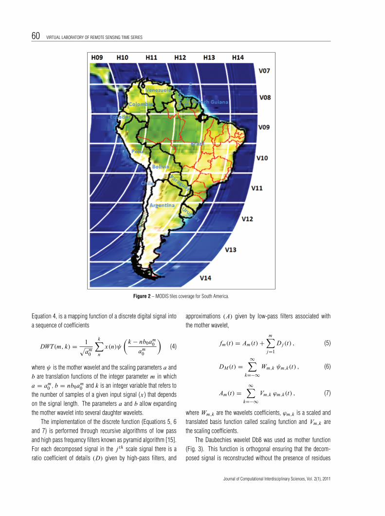
The present work was developed for the South America conti-nent that comprises about 18 million km2, representing 12%of the Earth land surface. The region is characterized by differ-ent biomes such as tropical and seasonal forest, caatinga for-est, grassland, savanna and others (Global Change Biology SouthAmerica map [8]).

The MODIS images were acquired at the portal WarehouseInventory Search Tool WIST NASA (https://wist.echo.nasa.gov).The selected product was the MOD13Q1 (collection 5) whichis the composition of 16 days at spatial resolution of 250 m.The time frame of data acquisition is July 2000 to December2010. The study area is divided in 29 MODIS tiles with 1,200 ×1,200 km each as illustrated in Figure 2. A total of 6,293 tileswere acquired corresponding to 3.5 TB of raw data. The imagesare in sinusoidal projection (WGS84 datum). All bands were re-projected to the geographic coordinate system with the samedatum and converted from HDF (Hierarchical Data Format) toGeoTIFF format to ensure data portability among software. Thetotal storage capacity is approximately 295 GB for each timeseries per spectral band. The vegetation index chosen for thepresent study is the EVI2 (Enhanced Vegetation Index 2; [9])which highlights the land cover variations. It is computed usingthe surface reflectance of the Red and NIR (near infrared) bandsavailable in the MOD13Q1 product (Equation 1):

EVI2 = 2.5 ∗NIR − Red

(NIR + 2.4 ∗ Red + 1)(1)

In addition, the view zenith angle band and the blue band (sur-face reflectance) were used to pre-filter the MODIS time series asexplained in the next section.

2.2 Filtering Procedures

Optical remote sensing data are frequently affected by cloudcover and sensor noise that interfere in the ability to character-ize spatial-temporal land cover dynamics. In order to construct a

Journal of Computational Interdisciplinary Sciences, Vol. 2(1), 2011

“main” — 2011/7/30 — 11:41 — page 59 — #3

RAMON MORAIS DE FREITAS et al. 59

Figure 1 – Virtual Laboratory of Remote Sensing Time Series framework.

continuous and consistent time series it is necessary to filter thedata. The filtering procedures were performed in two steps gen-erating two EVI2 time series: 1) without wavelet transform; and2) with wavelet transform. The first filtering procedure appliedrules that were designed following the methodologies proposedby [10, 11] in which data were eliminated from the original timeseries if the reflectance in the blue band is greater than 10% or ifthe sensor view zenith angle is greater than 32.5◦. These thresh-old procedures eliminate clouds contaminated and off-nadirpixels. The filtered data were then linear interpolated based onthe date of the pixel of the image composition to provide equallyspaced time series.

Further filtering was applies in the second filtering proce-dure using the wavelet transform following the methodology pro-posed by [12]. The signal decomposition by wavelets eliminatesthe high frequencies typically associated with the presence of

noise. The wavelet transform is given by [13, 14]:

W (a, b) =

+∞∫

−∞

f (t)1

√|a|ψa,b ∗

(t − b

a

)dt (2)

ψa,b(t) ≡1

√aψ(t − b)

a, a > 0, −∞ < b < +∞ (3)

where a is the scale parameter, b is the translation parameter,f (t) is the function to be transformed and ψ∗ is the motherwavelet function complex conjugate. The function (Equations 2and 3) is not continuous; therefore, it needs to be discretizedby using discrete values of (a, b) = (2m, 2n, k), where m,n and k are integer values and limited by the length of the timeseries. This allows the expansion of the mother wavelet to otherscales. The Discrete Wavelet Transform (DWT) decomposes adiscrete signal at different resolution levels. A DWT, defined in


“main” — 2011/7/30 — 11:41 — page 60 — #4


Figure 2 – MODIS tiles coverage for South America.

Equation 4, is a mapping function of a discrete digital signal intoa sequence of coefficients

DWT(m, k) =1

√am

0

k∑

n

x(n)ψ(

k − nb0am0

am0

)(4)

where ψ is the mother wavelet and the scaling parameters a andb are translation functions of the integer parameter m in whicha = am

0 , b = nb0am0 and k is an integer variable that refers to

the number of samples of a given input signal (x ) that dependson the signal length. The parameters a and b allow expandingthe mother wavelet into several daughter wavelets.

The implementation of the discrete function (Equations 5, 6and 7) is performed through recursive algorithms of low passand high pass frequency filters known as pyramid algorithm [15].For each decomposed signal in the j th scale signal there is aratio coefficient of details (D) given by high-pass filters, and

approximations (A) given by low-pass filters associated withthe mother wavelet,

fm(t) = Am(t)+m∑

j=1

D j (t) , (5)

DM (t) =∞∑

k=−∞

Wm,k ψm,k(t) , (6)

Am(t) =∞∑

k=−∞

Vm,k ϕm,k(t) , (7)

where Wm,k are the wavelets coefficients, ϕm,k is a scaled andtranslated basis function called scaling function and Vm,k arethe scaling coefficients.

The Daubechies wavelet Db8 was used as mother function(Fig. 3). This function is orthogonal ensuring that the decom-posed signal is reconstructed without the presence of residues


“main” — 2011/7/30 — 11:41 — page 61 — #5


Figure 3 – Wavelets functions: a) Db8 mother wavelet (ψ) and b) Scale function Db8 (ϕ).

due to asymmetries of the wavelet mother function. In this proce-dure, each set of pixels corresponds to a time series profile of thestacked images. The vector t was broken into 8 different scalesand the time series was reconstructed using the five largest scalescorresponding to lower frequencies. The higher frequencies wereeliminated because they are usually associated with the presenceof sensor noise and spectral responses contaminated by cloudsand shadows.

The names given to the two EVI2 time series generated by thefiltering procedures were:

1) without wavelet , and

2) with wavelet .

2.3 Data Integration and the Web Tool

The generated Data set (Fig. 1) is composed by over 500 millionEVI2 time series filtered with and without wavelet transform forthe entire South America continent. In order to construct this dataset a significant computational effort was carried out involvingmore than 60 days of processing time using three personal com-puters (PC) with Linux OS. All computational procedures usedMatlab and Ansi C platforms.

The EVI2 time series were integrated into the virtual globe(GoogleMaps) using the Dataset manager (Fig. 1) that was spe-cifically developed for this purpose. To visualize the EVI2 timeseries in the virtual globe a website was built, which is availableat http://www.dsr.inpe.br/laf/series.html, based on JavaScript andPHP platforms using Google Maps and Google Visualization

Application Programming Interface functionalities. For each callof a geographic coordinate from the virtual globe the two EVI2time series are instantaneously recovered. The information ofthe time series recovered by the call refers to one MODIS pixel.The integration with the virtual globe shows static geographicalspace using high spatial resolution satellite images provided byGoogle Maps server (Fig. 4a). However, caution should be takenfor analyzing these time series due to the different spatial reso-lution of the images. Each MODIS pixel represents roughly anarea of 6.25 ha (250 × 250 m) while the high spatial resolu-tion image provided by Google Maps is only used to locate theMODIS pixel. In addition, a tool was build to assess the ele-vation anisotropy around the selected point (red balloon). Thistool uses the elevation model information available in the Googlemaps API. The anisotropy visualization is a simple polar plot ofelevation around two sample circles, allowing a rapid view ofthe topography around the selected point (Fig. 4c). This toolallows interactivity and provides a range of distance betweenthe center of the selected coordinate and the sampled circles.Figure 4d shows the 10 years EVI2 time series using interac-tive plot provided by Google charts API functionalities. The redand blue lines represent the time series filtered with wavelet andwithout wavelet , respectively.

3 APPLICATIONS

The intense anthropogenic pressure forces the LULC changeprocesses in South America by converting natural forest andsavanna areas to pasture and agriculture. At sub-tropical region


“main” — 2011/7/30 — 11:41 — page 62 — #6


Figure 4 – Website display components: a) Google earth virtual globe used to select the geographic coordinate of the area of interest; b) list of selected points;c) polar plot of elevation around two sampled circles showed in Google image; and d) EVI time series for the selected plot (red line filtered with wavelet and blueline filtered without wavelet ).

there is the intensification of agriculture related to food and bio-fuels production [16, 17]. In this context some application exam-ples are provided using the visualization module described in thepresent work for LULC change analysis.

3.1 Land Use and Land Cover Change Over Forest

Figure 5a shows a forested region with several deforested areasin the municipality of Feliz Natal in Mato Grosso state, Brazil.The elevation around the selected point (11◦55′S; 54◦10′W)varies from 354 to 360 m indicating a reasonable flat terrain(Fig. 5b). The MODIS EVI2 time series are presented in Figure5c. Analyzing the time series a decrease in the EVI2 values canbe observed in 2004 indicating a significant biomass loss dueto the deforestation process. From 2005 to 2007 there was al-most no vegetation regrowth as indicated by the low EVI2 pro-

file during this period. For the years of 2007 and 2008 a typicalspectral response for agricultural areas can be observed, charac-terized by a rapid increase followed by a rapid decrease of thevegetation index values indicating the well defined and shortgrowth cycles of agricultural annual crops.

Figure 6 shows the seasonality of a selected point froman area that was deforested in 2004 in the National Park ofXingu, Mato Grosso state, Brazil. The visual analysis of the timeseries indicates a land conversion from forest to pastures. Itcan also be observed that the deforestation process started inthe first quarter of 2004 and ended in the last quarter of thesame year. It is interesting to note that the two areas observedin Figures 5 and 6 present different types of land use changethat can be easily observed by analyzing the 10 years MODISEVI2 time series. The double arrows illustrate the land use or landcover in the period.


“main” — 2011/7/30 — 11:41 — page 63 — #7


Figure 5 – a) GoogleMaps image; b) elevation polar plot; and c) EVI2 time series plot for the selected coordinated point.

It is also interesting to note that the two differently filteredEVI2 time series generated similar curves for the selected plots ofFigures 5c and 6c. A smoother curve is observed for the EVI2 withwavelet (red curve), and but no significant difference is observedfor the without wavelet (blue curve) in terms of LULC changeanalysis. On the other hand the smoothed filtered EVI2 time se-ries can be used in the data mining and other classification pro-cedures when the high frequency signal is not interesting.

3.2 Land Use and Land Cover Change Over Sugarcane

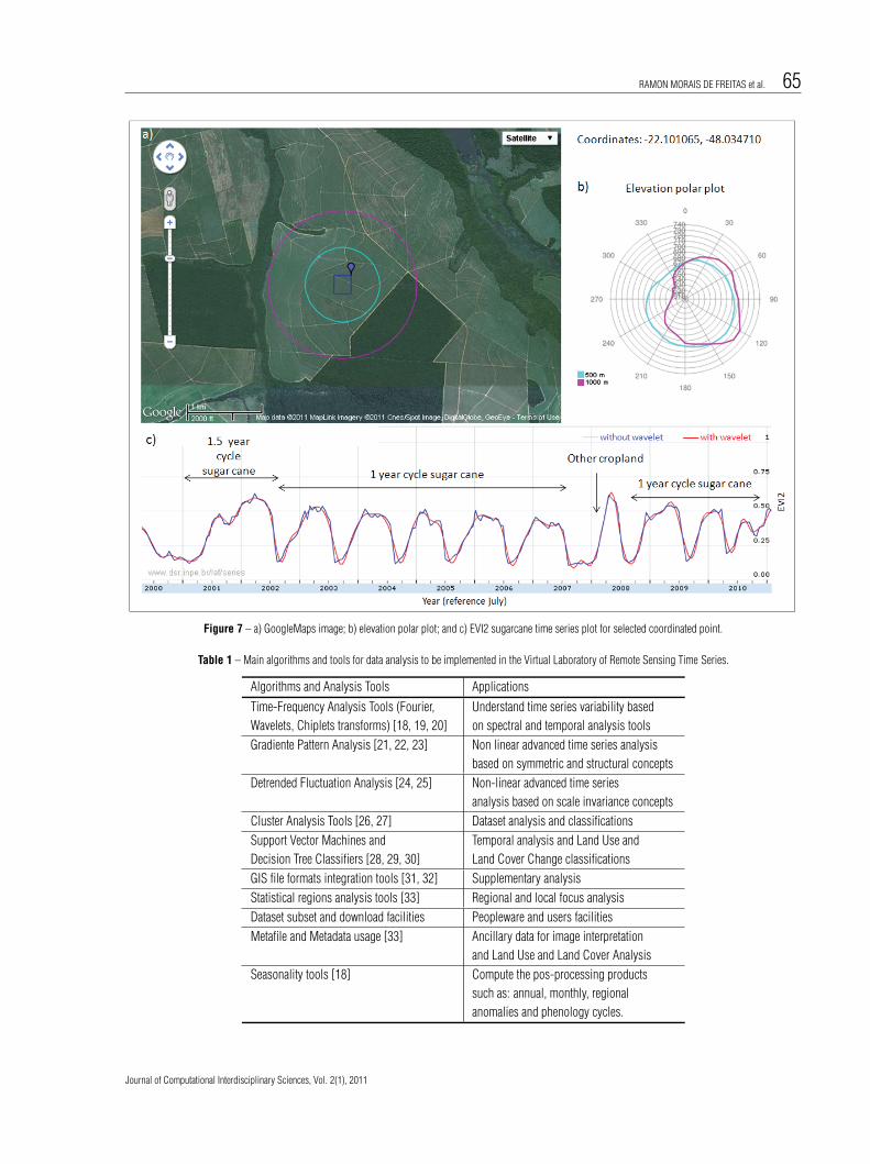
Figure 7a shows a region with intense sugarcane cultivation in themunicipality of Brotas, Sao Paulo state, Brazil. Figure 7c showsthe dynamic of nine sugarcane crop years. With some knowledgeon sugarcane cultivation several information can be extractedfrom the time series curve. A brief description of the sugarcanecultivation practices in this area can be given by the analyst inthe following form. At the very beginning of the time series thelow EVI2 values indicate bare soil over which the sugarcane was

planted in the beginning of 2001. This sugarcane plant grew forabout 18 months when it was harvested for the first time aroundJuly 2002. After the first cut the sugarcane ratoons were harvestedonce a year, around July, from 2003 to 2007. The sugarcane fieldwas renovated in late 2007 when it was rotated with an annualsummer crop followed by new sugarcane planted in late 2008 andharvested in mid 2009. More information about this plot can beobtained at http://www.dsr.inpe.br/laf/canasat/ [17].

The above description indicated that with a minimum of tech-nical knowledge about sugarcane agricultural practices it is pos-sible to the analyst recovering the 10 years history of specific plotsand fields. This can be of great interest to certifiers that need toknow the LULC change history.

3.3 Land Use and Land Cover Change Over Savanna

Figure 8 shows an agricultural region at the frontier of the sa-vanna located in western Bahia state, Brazil. The region wasoriginally covered by savanna and has been gradually converted


“main” — 2011/7/30 — 11:41 — page 64 — #8


Figure 6 – a) GoogleMaps image; b) elevation polar plot; and c) EVI2 time series plot for selected coordinated point.

to intense agricultural land use. This region is characterized bylarge soybeans, corn, cotton and coffee plantations. Three timeseries over typical plots can be observed in Figures 8c, 8d and8e. Figure 8c shows the typical behavior of a savanna with rel-ative low values EVI2 and small amplitudes. Figure 8d presentsthe curve of a savanna area which was converted to agricultureduring the 2007/2008 crop season. Figure 8e shows the conver-sion of savanna to agriculture after 2002.

4 GENERAL REMARKS AND FUTURE WORKS

This work presented a visualization module for the virtual labor-atory using the ten years history of MODIS EVI2 time seriesfor the entire South America continent. The visualization mod-ule demonstrated to be useful for rapid land use and land coverchange analysis, at the pixel level, over large regions. Thesmoothed filtered EVI2 time series using wavelet transformationcould be used for checking dates of land use change such as date

of deforestation, planting date of agricultural crops, seasonal ef-fect on pasture land and others. Regarding to the integration withvirtual globes such as Googlemaps, this work showed an innova-tion because it allows the public access and instantaneous visu-alization. This work can be extended for any geographical regionsince MODIS data are available for the entire globe.

Future works will be focused on providing quality parametersassociated with each time-series, through an under-developmentvalidation procedure. Due to the area coverage, a near-real timeopen access techniques will be evaluated for allowing land covertypes to be detected by any analyst with a GPS. Table 1 describesthe main algorithms and tools for data analysis to be implementedin future virtual laboratory versions. A user friendely interface willbe implemented to connect the Algorithm module and the Ana-lysis module facilities with virtual laboratory users.

Next versions of the Virtual Laboratory of Remote SensingTime Series can be implemented with other data sets such as tem-perature, rainfall, fraction components of linear mixture model and


“main” — 2011/7/30 — 11:41 — page 65 — #9


Figure 7 – a) GoogleMaps image; b) elevation polar plot; and c) EVI2 sugarcane time series plot for selected coordinated point.

Table 1 – Main algorithms and tools for data analysis to be implemented in the Virtual Laboratory of Remote Sensing Time Series.

Algorithms and Analysis Tools Applications

Time-Frequency Analysis Tools (Fourier,

Wavelets, Chiplets transforms) [18, 19, 20]

Understand time series variability based

on spectral and temporal analysis tools

Gradiente Pattern Analysis [21, 22, 23] Non linear advanced time series analysis

based on symmetric and structural concepts

Detrended Fluctuation Analysis [24, 25] Non-linear advanced time series

analysis based on scale invariance concepts

Cluster Analysis Tools [26, 27] Dataset analysis and classifications

Support Vector Machines and

Decision Tree Classifiers [28, 29, 30]

Temporal analysis and Land Use and

Land Cover Change classifications

GIS file formats integration tools [31, 32] Supplementary analysis

Statistical regions analysis tools [33] Regional and local focus analysis

Dataset subset and download facilities Peopleware and users facilities

Metafile and Metadata usage [33] Ancillary data for image interpretation

and Land Use and Land Cover Analysis

Seasonality tools [18] Compute the pos-processing products

such as: annual, monthly, regional

anomalies and phenology cycles.


“main” — 2011/7/30 — 11:41 — page 66 — #10


Figure 8 – a) GoogleMaps image; b) elevation polar plot; c) EVI2 time series plot for selected coordinated point 1, savanna area; d) EVI2 time series plot for selectedcoordinated point 2, deforestation area in 2007; and e) EVI2 time series plot for selected coordinated point 3, deforestation area in 2002.


“main” — 2011/7/30 — 11:41 — page 67 — #11


vegetation indices. The concept, protocols, hardware support andother software engineering specifications have been carried out tomake the instantaneous visualization and analysis of time seriesa reality for remote sensing and general GIS users community.

ACKNOWLEDGMENTS

The authors thank CAPES (Coordenacao de Aperfeicoamento dePessoal de Nıvel Superior), FAPESP (Fundacao de Amparo aPesquisa do Estado de Sao Paulo) and CNPq (Conselho Nacionalde Desenvolvimento Cientıfico e Tecnologico) agencies for par-tial financial support to the work, and INPE (Earth Observation –OBT, Remote Sensing Division, DSR and Laboratory of Agricul-ture and Forest – LAF) for infrastructure and computing support.The MODIS data are distributed by the Land Processes DistributedActive Archive Center (LP DAAC), located at the U.S. GeologicalSurvey (USGS) Earth Resources Observation and Science (EROS)Center (lpdaac.usgs.gov). The author thanks the referees for theirhelpful suggestions concerning the presentation of this paper.

REFERENCES

[1] LAMBIN EF & LINDERMAN M. 2006. Time series of remote sens-

ing data for land change science. IEEE Transactions on Geoscience

and Remote Sensing, 44(7): 1926–1928.

[2] DEFRIES RS, ASNER GP & HOUGHTON RA. 2004. Ecosystems and

Land Use Change. American Geophysical Union, Washington, DC.

[3] JUSTICE CO, TOWNSHEND JRG, VERMOTE EF, MASUOKA E,

WOLFE RE, SALEOUS, N, ROY DP & MORISETTE JT. 2002. An

overview of MODIS Land data processing and product status. Re-

mote Sensing of Environment, 83: 3–15.

[4] BUTLER D. 2006. Virtual globes: the web-wide world. Nature,

439(7078): 776–778.

[5] BALLAGH LM, RAUP BH, DUERR RE, KHALSA SJS, HELM C,

FOWLER D & GUPTE A. 2011. Representing scientific data sets

in KML: Methods and challenges, Computers & Geosciences,

37(1), Virtual Globes in Science, p. 57–64. ISSN 0098-3004,

DOI: 10.1016/j.cageo.2010.05.004.

[6] CHIANG G, TOBY OH, DOVE MT, BOVOLO CI & EWEN J. 2011.

Geo-visualization Fortran library, Computers & Geosciences,

37(1), Virtual Globes in Science, p. 65–74, ISSN 0098-3004,

DOI: 10.1016/j.cageo.2010.04.012.

[7] NIELSON GM. 1991. Visualization in Scientific and Engineering

Computation. IEEE Computer, 24(9): 58–66.

[8] EVA H, BELWARD A, EVARISTO M, DI BELLA C, GOND V, JONES

S, SGRENZAROLI M & FRITZ S. 2004. A land cover map of South

America, Global Change Biology, 10: 731–744.

[9] JIANG Z, HUETE AR, DIDAN K & MIURA T. 2008. Development

of a two-band Enhanced Vegetation Index without a blue band.

Remote Sensing of Environment, 112(10): 3833–3845.

[10] SAKAMOTO T, YOKOZAWA M, TORITANI H, SHIBAYAMA M,

ISHITSUKA N & OHNO H. 2005. A crop phenology detection

method using time series MODIS data. Remote Sensing of Envi-

ronment, 96(3-4): 366–374.

[11] THAYN JB & PRICE KP. 2008. Julian dates and introduced tempo-

ral error in remote sensing vegetation phenology studies. Interna-

tional Journal of Remote Sensing, 29: 6045–6049.

[12] FREITAS RM & SHIMABUKURO YE. 2008. Combining wavelets

and linear spectral mixture model for MODIS satellite sensor time

series analysis. JCIS – Journal of Computational Interdisciplinary

Sciences, 1: 51–56.

[13] DAUBECHIES I. 1992. Ten lectures on wavelets. CBMS-NSF Re-

gional Conference Series in Applied Mathematics 61, Philadelphia,

PA. Soc. Ind. Appl. Math, 377 pp.

[14] MEYER Y. 1992. Wavelets and operators, Cambridge Studies in

Advanced Math., vol. 37, Cambridge Univ. Press, Cambridge, 223

p.

[15] MALLAT S. 1989. A theory for multi resolution signal decompo-

sition: the wavelet representation. IEEE Transactions on Pattern

Analysis and Machine Intelligence, 11: 674–693.

[16] LAPOLA DM, SCHALDACH R, ALCAMO J, BONDEAU A, KOCH J,

KOELKING C & PRIESS JA. 2010. Indirect land-use changes can

overcome carbon savings from biofuels in Brazil. Proceedings of

the National Academy of Sciences, 107(8): 3388–3393.

[17] RUDORFF BFT, AGUIAR DA, SILVA WF, SUGAWARA LM, ADAMI

M & MOREIRA MA. 2010. Studies on the Rapid Expansion of

Sugarcane for Ethanol Production in Sao Paulo State (Brazil) Using

Landsat Data. Remote Sensing, 2: 1057–1076.

[18] MALLAT S. 1999. A wavelet tour of signal processing, 2nd Edition,

Academic Press.

[19] LE PENNEC E & MALLAT S. 2005. Sparse Geometric Image Repre-

sentation with Bandelets, IEEE Trans. on Image Processing, 14(4):

423–438.

[20] BOASHASH B. 2003. Time-Frequency Signal Analysis and Pro-

cessing: A Comprehensive Reference, Oxford: Elsevier Science.

[21] ROSA RR, PONTES J, CHRISTOV CI, RAMOS FM, RODRIGUES

NETO C, REMPEL EL & WALGRAEF D. 2000. Physica A, 283: 156.

[22] ASSIREU AT, ROSA RR, VIJAYKUMAR NL & LORENZZETTI JA.

2002. Gradient pattern analysis of short nonstationary time series:

an application to Lagrangian data from satellite tracked drifters.

Physica D, Elsevier, 169c: 397–403.


“main” — 2011/7/30 — 11:41 — page 68 — #12


[23] FREITAS RM, ROSA RR & SHIMABUKURO YE. 2010. Using Gra-

dient Pattern Analysis for land use and land cover change detec-

tion. In: International Geoscience and Remote Sensing Symposium

(IGARSS), IEEE, Honolulu, 1: 3648–3651.

[24] PENG CK et al. 1994. Mosaic organization of DNA nucleotides.

Phys Rev E, 49(2): 1685–1689.

[25] KANTELHARDT JW et al. 2001. Detecting long-range correlations

with detrended fluctuation analysis. Phys A, 295(3-4): 441–454.

[26] DUDA RO, HART PE. 1973. Pattern Classification and Scene, Ana-

lysis, New York: John Wiley & Sons, Inc.

[27] HARTIGAN JA. 1985. Statistical Theory in Clustering. Journal of

Classification, 2: 63–76.

[28] THEODORIDIS S, KOUTROUMBAS K. 2009. Pattern Recognition,

4th Edition, Academic Press.

[29] YANG T. 2006. Computational Verb Decision Trees. International

Journal of Computational Cognition (Yang’s Scientific Press), 4(4):

34–46.

[30] YUAN Y, SHAW MJ. 1995. Induction of fuzzy decision trees. Fuzzy

Sets and Systems, 69: 125–139.

[31] LONGLEY P, GOODCHILD MF, MAGUIRE DJ, RHIND DW. 2005.

Geographical information systems and science: John Wiley &

Sons Inc.

[32] LONGLEY P. 2008. To what extent are the fundamental spatial con-

cepts that lie behind GIS relevant in design? In Spatial Concepts

in GIS and Design. Santa Barbara, CA: UCSB.

[33] BRETHERTON FP, SINGLEY PT. 1994. Metadata: A User’s View,

Proceedings of the International Conference on Very Large Data

Bases (VLDB). pp. 1091–1094.


virtual laboratory of remote sensing time series: visualization … · virtual laboratory of remote...

Documents