vitaliy pipich ordering transition and critical phenomena ... · 2.3.2 eﬀect of thermal ... in...

Vitaliy Pipich

Ordering Transition and Critical Phenomena

in a three Component Polymer Mixture of

A/B Homopolymers and

a A-B Diblockcopolymer

2003

Physikalische Chemie

Ordering Transition and Critical Phenomena

in a three Component Polymer Mixture of

A/B Homopolymers and

a A-B Diblockcopolymer

Inaugural-Dissertation

zur Erlangung des Doktorgrades der Naturwissenschaftenim Fachbereich Chemie und Pharmazie

der Mathematisch-Naturwissenschaftlichen Fakultatder Westfalischen Wilhelms-Universitat Munster

vorgelegt von

Vitaliy Pipich

aus Chmelnitskiy, Ukraine

- 2003 -

Dekan: Prof. Dr. Jens Leker

Erster Gutachter: Prof. Dr. Dieter Richter

Zweiter Gutachter: Prof. Dr. Andreas Heuer

Tag der mundlichen Prufungen: 26.03, 30.03, 06.04.2004

Tag der Promotion: 30.04.2004

Contents

1 Introduction 1

2 Theory 5

2.1 Ginzburg-Landau-Wilson Hamiltonian . . . . . . . . . . . . . . . 5

2.2 Mean Field Phase Diagram of A/B/A-B Blends . . . . . . . . . . 10

2.3 Polymer Blends: A/B . . . . . . . . . . . . . . . . . . . . . . . . . 13

2.3.1 Thermodynamics of Polymer Blends: Critical Behavior –

Flory-Huggins Theory . . . . . . . . . . . . . . . . . . . . 13

2.3.2 Effect of Thermal Fluctuations: A/B blends . . . . . . . . 15

2.3.3 Belyakov-Kiselev Crossover Model . . . . . . . . . . . . . . 16

2.4 Diblock Copolymer Melts . . . . . . . . . . . . . . . . . . . . . . 17

2.4.1 Thermodynamics of Block Copolymers . . . . . . . . . . . 17

2.4.2 RPA: A-B melts . . . . . . . . . . . . . . . . . . . . . . . . 17

2.4.3 Effect of Thermal Fluctuations: A-B melts . . . . . . . . . 18

2.5 A/B/A-B . . . . . . . . . . . . . . . . . . . . . . . . . . . . . . . 19

2.5.1 RPA of the Ternary A/B/A-B System . . . . . . . . . . . 19

2.5.2 Effect of Thermal Fluctuations:A/B/A-B . . . . . . . . . . 21

2.5.3 Scaling Behavior . . . . . . . . . . . . . . . . . . . . . . . 24

2.6 Polymeric Microemulsion . . . . . . . . . . . . . . . . . . . . . . . 26

3 Experimental 29

3.1 Sample . . . . . . . . . . . . . . . . . . . . . . . . . . . . . . . . . 29

i

ii CONTENTS

3.1.1 Polymer Synthesis and Characterization . . . . . . . . . . 29

3.1.2 Sample Preparation . . . . . . . . . . . . . . . . . . . . . . 31

3.1.3 Thermostat . . . . . . . . . . . . . . . . . . . . . . . . . . 32

3.2 Small Angle Neutron Scattering . . . . . . . . . . . . . . . . . . . 34

3.2.1 Basics of Small Angle Neutron Scattering . . . . . . . . . . 34

3.2.2 Raw Data Reduction . . . . . . . . . . . . . . . . . . . . . 36

3.2.3 Dead Time Effect . . . . . . . . . . . . . . . . . . . . . . . 37

3.2.4 Resolution Function . . . . . . . . . . . . . . . . . . . . . 38

4 Experimental results 41

4.1 Phase Diagram . . . . . . . . . . . . . . . . . . . . . . . . . . . . 41

4.1.1 Lifshitz Line . . . . . . . . . . . . . . . . . . . . . . . . . . 41

4.1.2 Disorder Line . . . . . . . . . . . . . . . . . . . . . . . . . 46

4.1.3 Microemulsion Phases . . . . . . . . . . . . . . . . . . . . 47

4.1.4 Temperature Induced Disorder–Microemulsion Transition . 49

4.1.5 Lamellar - Bicontinuous Microemulsion Transition . . . . . 52

4.1.6 Order-Disorder Transition of the Diblock Copolymer melt 53

4.1.7 Ordering Transition in A/B/A-B Blend . . . . . . . . . . . 53

4.1.8 Phase Diagram in Different Contrasts . . . . . . . . . . . 55

4.2 Critical Exponents and Crossover . . . . . . . . . . . . . . . . . . 59

4.2.1 Ising Critical Behavior . . . . . . . . . . . . . . . . . . . . 59

4.2.2 Lifshitz Critical Behavior . . . . . . . . . . . . . . . . . . . 64

4.2.3 Reentrance Behavior and Double Critical Point . . . . . . 66

4.3 Role of the Diblock Copolymer . . . . . . . . . . . . . . . . . . . 68

5 Interpretation of the Data 73

5.1 S(Q) and S(Q∗) below the LL (Φ < ΦLL) . . . . . . . . . . . . . . 73

5.2 S(Q) and S(Q∗) beyond the LL (Φ > ΦLL) . . . . . . . . . . . . . 76

5.3 S(Q) and S(0) near the LL . . . . . . . . . . . . . . . . . . . . . 79

CONTENTS iii

6 Discussion 83

6.1 Critical Exponents: Critical Path . . . . . . . . . . . . . . . . . . 83

6.2 Disordered and Microemulsion Lifshitz Line. Bicontinuous and

Droplet Microemulsion . . . . . . . . . . . . . . . . . . . . . . . . 86

6.3 Gi and Microemulsion channel . . . . . . . . . . . . . . . . . . . . 87

6.4 Flory-Huggins Parameter . . . . . . . . . . . . . . . . . . . . . . . 88

7 Conclusions 91

List of Figures 96

List of Tables 100

Bibliography 102

Acknowledgments 109

CV(Lebenslauf) 111

iv CONTENTS

Chapter 1

Introduction

Phase separation and critical anomalies of thermal composition fluctuations inbinary polymer blends are well-known universal phenomena which have been in-tensively explored both from a theoretical and experimental point of view [1].Usually, the critical behavior of thermal fluctuations is discussed in terms ofuniversality classes and the crossover between them. Each universality class ischaracterized by a set of unique critical exponents describing thermodynamicparameters as the correlation length and susceptibility by scaling laws. At tem-peratures far from the critical point thermal fluctuations become very weak thatthey can be handled theoretically as individual fluctuation modes within the so-called Gaussian approximation. The critical exponents are in most cases identicalto those of the mean field case so that one usually identifies this regime as fulfillingthe mean field approximation.

Approaching the critical point fluctuations become stronger and non-lineareffects become apparent indicating a crossover to a different fluctuation dom-inated universality class. In the case of binary polymer blends one gets thecrossover to the university class of the 3D-Ising model [2, 3]. Such a crossoveris estimated by a Ginzburg criterion [3, 4] delivering a Ginzburg number Gi,representing a reduced temperature which for binary polymer blends is propor-tional to N−1, N being degree of polymerization. The Ginzburg number deter-mines the temperature interval of strong thermal fluctuations around the crit-ical point. Such a universal Ginzburg criterion is only valid for incompressiblepolymer blends [1,5]. The crossover behavior of the susceptibility and correlationlength from mean field to 3D-Ising critical behavior can be described by crossovermodels [6, 7].

The critical behavior of polymer blends can be quite differently influencedby the microstructure of the polymer, by external pressure fields, and additivesas solvent molecules [8, 9, 10]. So, the covalent binding of two homopolymers toa diblock copolymer leads to a crossover from 3D-Ising to the Brasovskii univer-sality class which shows much stronger fluctuation effects [11,12] and a Ginzburgnumber Gi, being proportional to N−1/2. One consequence for symmetric diblock

1

2 CHAPTER 1. INTRODUCTION

copolymers is a characteristic change of the disorder-order phase transition fromsecond-order to weak first-order. Another situation appears in the presence of athird component which could affect the critical behavior due to fluctuations ofdensity. Fisher’s renormalized Ising model describes such an “impurity” effect byincreasing the Ising critical exponents by a factor of 1/(1−(α)) [13,14]. Here, α isthe critical exponent of the specific heat of the Ising system. In other cases, struc-tural changes of the polymers or external pressure fields influence “non-universal”critical parameters as the critical temperature TC and the Ginzburg number Gi.So, pressure usually leads to a reduced Ginzburg number [9, 10].

In this study small angle neutron scattering (SANS) studies on a binaryA,B homopolymer mixture of critical composition mixed with a symmetric A-B diblock copolymer are presented. These A-B diblock copolymers act as ansurfactant molecules reducing the surface energy and thereby leading to an im-proved miscibility and to stronger thermal fluctuations. But, as homopolymerblends and diblock copolymers obey different universality classes blending leadsto new phenomena as the universality class of the isotropic Lifshitz case and tomicroemulsion phases. Mean field theory predicts a Lifshitz critical point and insome cases even a Lifshitz tricritical point [15] with the critical exponents γ =1and ν = 1/4 of susceptibility and correlation length, respectively. Those meanfield critical exponents were observed in such a system of rather large polymermass [16]. Another related study on a mixture of significantly reduced poly-mer mass gave a sharp transition with increasing diblock content from 3D-Ising(γ = 1.24, ν = 0.63) to the isotropic Lifshitz critical exponents of (γ = 1.62 andν = 0.9) [17,18]. These studies have shown that thermal composition fluctuationsplay an important role in the range of the Lifshitz universality class. Due to thevanishing surface energy which acts as a restoring force for the fluctuations andleads to a scaling behavior of Ginzburg number according to N−2/3 [15]. Thesestrong fluctuations are responsible for several deviations from the mean fieldpredicted phase behavior: (1) No Lifshitz critical point is observed and a microemulsion channel appears between the two-phase and lamellar phase regimes [19];(2) the Lifshitz Line shows a non-monotonic temperature dependence [18].

The present studies were mainly focused on the regime of the Lifshitz crit-ical behavior. We made new observations from which we hope to further clarifythe phase behavior, especially in this range. So, within a narrow range of diblockconcentration between 6 and 12% a closed-loop two-phase regime terminated bya double critical point and a droplet and bicontinuous microemulsion phase wasobserved. The border line, where the correlations of the bicontinuous microemul-sion phase becomes visible, appears as the lower temperature continuation of theLifshitz line.

Samples with three different scattering contrasts were explored in order tobetter understand the behavior of the diblock copolymer. This was done bymeasuring the fluctuations between all the A and B monomers, irrespectively,whether they originate from the homopolymer or the block copolymer (bulk con-

3

trast); from one block of the diblock copolymer (block contrast) and in the othercase only from the middle part of the diblock copolymer (film contrast). In neu-tron scattering such conditions of changing contrast are relatively easily achievedfrom the exchange of hydrogen and deuterium during the synthesis of the poly-mers.

4 CHAPTER 1. INTRODUCTION

Chapter 2

Theory

2.1 Ginzburg-Landau-Wilson Hamiltonian

We investigated a ternary polymer mixture consisting of a binary polymer blendof Polybutadiene (PB) and Polystyrene (PS) of critical composition and of thecorresponding symmetrical PB-PS diblock copolymer of varying concentrations.In order to get the ordering phase transitions of the blend and the diblockcopoly-mer in the same temperature range the molar volume of the diblock copolymerwas about six times larger than those of the homopolymers. In order to measurethe “component” fluctuations with a strong scattering contrast, for most of SANSstudies, the PB and PS were deuterated and protonated, respectively (so-called“bulk” contrast). Thermal composition fluctuations with respect to the totalmonomer fractions correspond to a scalar (n = 1) order parameter representedby the local concentration of the PB or PS component Φ = Φ(x). The com-mon Landau expansion describes the basic thermodynamic features sufficientlywell within mean field approximation of those systems near their consolute lineaccording to the Hamiltonian [20, 21],

H =1

2

∫

ddx(

c2(~∇Φ)2 + c4(~∇Φ)4 + rΦ2 + uΦ4 + u6Φ6)

. (2.1)

An ordinary critical point (for example a demixing point) occurs when thesusceptibility r becomes zero, and the other parameters are positive. An ordinarytricritical point(when three phases coexist) occurs when r = 0 and u = 0, with theother parameters positive. At a Lifshitz critical point, r = c2 = 0 and similarly ata Lifshitz tricritical point, r = u = c2 = 0, with all the other parameters positive.

A Lifshitz critical point and a Lifshitz line generally appear in those systemswith competing tendencies for phase separation into bulk and spatially modulatedphases. When the appropriate parameter controlling the relative strength ofthe two tendencies is varied along the critical line of phase transitions a special

5

6 CHAPTER 2. THEORY

Table 2.1: Mean field definitions of characteristic points. The parame-ters of the second column will be defined later.

Type of CP Hamiltonianparameters

Structure Factorsparameters

Critical Solution Point r−1 = 0 S−1(0) = 0

Lifshitz Point c2 = 0 L2 = 0

Lifshitz Critical Point r−1 = 0c2 = 0

S−1(0) = 0L2 = 0

Tricritical Lifshitz Critical Point r−1 = 0c2 = 0u = 0

S−1(0) = 0L2 = 0

multi-critical point occurs at which the character of phase separation undergoesa change from bulk phase separation to the phase separation into a spatiallymodulated phase. The Lifshitz point is known to exist in magnetic systems[21, 22, 23, 24], liquid crystals [25], polyelectrolytes [26, 27], oil/ water/surfactantmixtures [28], random block-copolymers [29, 30], and mixtures of homopolymersand diblock copolymers [15, 31]. In the paper by Kudlay and Semenow in ref.[32] a theoretical description of the behavior of the Lifshitz line with varyingtemperature is developed and it was shown that the wave vector dependence ofthe fluctuation corrections is responsible for the experimentally observable non-linearity of the Lifshitz line.

Homopolymer blends are sufficiently well described by the Hamiltonian withc4 = 0 and u6 = 0 (Φ4 model). A third component can influence on the Hamil-tonian by reducing the u-parameter.

A principal effect of an (A-B) diblock copolymer dissolved in an (A/B)homopolymer blend is the reduction of the surface energy which according to theHamiltonian, in Eq. 2.1, is described by a reduction of the parameter c2. Thisparameter is positive at low copolymer content, becomes zero at the concentrationof the Lifshitz line, and negative for larger copolymer content. The Hamiltonianaccounts for the composition fluctuations in the homogeneous (disordered) one-phase regime. The composition fluctuations are described by the structure factorS(Q), Q being the momentum transfer, and is measured directly in a scatteringexperiment (Q = 4π

λsin Θ, where λ and Θ is the wavelength of the used radiation

and the half of the scattering angle,respectively).

Positive c2-values demonstrate the characteristic behavior of polymer blends;S(Q) is maximum at Q = 0, and the susceptibility, r−1, is correspondingly given

2.1. GINZBURG-LANDAU-WILSON HAMILTONIAN 7

by S(Q = 0),r−1 = S(0). (2.2)

At the critical temperature Tc of macrophase separation the susceptibilitydiverges and the inverse susceptibility S−1(0) becomes zero. For negative c2-values the structure factor, S(Q), has the basic characteristics of block copolymermelts, the maximum value of S(Q) appears at a finite Q-value, Q = Q∗. Thesusceptibility is then given by the structure factor at this Q∗-value. Accordingto the mean field theory of symmetric copolymers additives, the susceptibilityS(Q∗) diverges at the order-disorder critical point, and orders on a mesoscopiclength scale beyond through microphase separation.

In mean field approximation the inverse structure factor S−1(Q) can beexpanded into powers of Q2. Considering the decrease of the surface energy withincreasing copolymer content the structure factor can be described by [15]

S−1(Q) = S−1(0) + L2Q2 + L4Q

4, (2.3)

where the coefficients L2 and L4 are proportional to the c2 and c4 terms in theHamiltonian Eq. 2.1, respectively.

The structure factor of a binary polymer blend demonstrates a Q−2 scalingdependence, described by an Ornstein-Zernike approach, which is equivalent toEq. 2.3 with L4=0. As diblock copolymer additives lead to a decrease of the roleof the c2-term in the Hamiltonian the c4-term becomes visible and dominant aswell as the L4-term in the structure factor; the disappearance of the c2 term leadsto a characteristic Lifshitz Q−4 behavior of the structure factor. In case of equalmolecular volumes of homopolymers and diblock copolymers mean field theorypredicts the existence of a tricritical Lifshitz point, where c2, u and r−1 becomezero.

Symmetric diblock copolymers modulate homopolymers on the local lengthscale like a surfactant does in a water-oil microemulsion. In analogy betweenwater-oil microemulsions and homopolymer - diblock copolymer blends withinmean field approximation both systems are characterized by the same structurefactor Eq. 2.3. In order to explain the broad single peak profile of SANS pat-terns from oil-water microemulsion structures, Teubner and Strey [33] proposed asimple function derived from the phenomenological Ginzburg-Landau free energyfunctional (compare with given Hamiltonian in Fig. 2.1). The microemulsionstructure is characterized by an alternative distribution of water and oil domains,for which they introduced the following spatial correlation function,

g(r) ∼ exp

(

− r

ξTS

)

[

12πrλTS

sin(2πr

λTS

)

]

, (2.4)

where the domain periodicity λTS and the correlation length ξTS are the tworelevant static length scales. The parameters λTS and ξTS are expressed in terms

8 CHAPTER 2. THEORY

of the structure factor parameters of Eq. 2.3 as

λTS = 2π

[

1

2

(

√

S−1(0)

L4− L2

2L4

)]−1/2

, (2.5)

ξTS =

[

1

2

(

√

S−1(0)

L4+

L2

2L4

)]−1/2

. (2.6)

In the limit λTS → ∞ the correlation function Eq. 2.4 demonstrates an expo-nential decay as binary blends. On the other hand, a periodic structure of theordered lamellar phase is described by Eq. 2.4 in the limit of ξTS → ∞. In meanfield approximation the disorder-order transition has second order characteristics,and thus the correlation length diverges at a order-disorder phase boundary.

In order to estimate the size distribution of the PB and PS domains itseems to be useful to use a disorder parameter Dm = λTS/(2πξTS) as proposedin Ref. [34]. The disorder parameter allows to make a definition of some phaselines

Dm =λTS

2πξTS=

= ∞ at the disorder line= 1 at the Lifshitz line= 0 at the lamellar phase boundary

Table 2.1 summarizes the characteristic lines and points of this system inmean field approximation.

Strey et al. [35, 36, 37] have further classified the differently structured flu-ids in the disordered phase of the oil/water/surfactant system by defining theamphiphilicity factor, fa, in terms of the structure factor parameters Eq. 2.3 as

fa =L2

√

4S−1(0)L4

, (2.7)

and extending the Teubner-Strey model over all ranges of amphiphilicity. Forstrong amphiphilicity with fa < −1, the microemulsion phase is unstable withrespect to the lamellar phase. With slightly less amphiphilicity, −1 < fa < 0, astrongly structured, “good” microemulsion phase results. The real “amphiphilic-ity” of systems increases as fa decreases. One distinguishing characteristics of a”good” microemulsion is the tendency to create a large interface area due to avanishing or negative microscopic surface tension. This corresponds to a negativevalue of L2, and thus negative fa. The line fa = 0 is the Lifshitz line of the mi-croemulsion (µLL). A further decrease in amphiphilicity, 0 < fa < 1, results in a”poor” microemulsion. Here, the correlation function g(r) is still oscillatory, butinterfacial correlations no longer dominate the scattering and the structure factorpeak occurs at zero wave vector. Finally, for fa > 1, the fluid has no structureand g(r) is no longer oscillatory. The boundaries between these classificationsdo not correspond to thermodynamic transitions, but are simply demarcations

2.1. GINZBURG-LANDAU-WILSON HAMILTONIAN 9

between differently structured fluids. The (water/water) Lifshitz line is definedby L2 = 0, and marks the boundary between ”good” and ”poor” microemulsions.The disorder line at fa = 1 signifies the transition from correlated to uncorrelatedinterfaces.

10 CHAPTER 2. THEORY

2.2 Mean Field Phase Diagram of A/B/A-B Blends

0 2 4 6 8 10 80 10020

40

60

80

100

120

140

160

Lifshitz Line(Homopolymer-homopolymer)

TODT

Disorder Line

Lifshitz Line(total)

Disordered "Homopolymer"

Disordered "Diblock Copolymer"

Lamella

Lifshitz Point

Mean-Field Phase Diagram

T[°

C]

Concentration Diblock [%]

Two-Phase

Tc

Figure 2.1: Phase diagram of the ternary mixture at equal concentrationsof A and B homopolymers as obtained from mean field theory. At low tem-peratures there exists a two-phase coexistence between A-rich and B-richphases at low copolymer concentrations, a lamellar phase at high concen-trations. The Lifshitz line divides the disordered phase to “homopolymer-like” and “copolymer-like” ranges.

Ternary mixtures of two partially incompatible homopolymers and a diblockcopolymer are in some respects similar to mixtures of oil, water, and amphiphile.But the copolymer is generally not so efficient as a solubilizer of the homopolymersas an amphiphile is for oil and water, because the homopolymer-homopolymerLifshitz line is far from the total Lifshitz line [15].

Mean field theory can predict the phase diagram for symmetric ternarysystems. The schematic phase diagram of A/B/A-B blends are shown in Fig. 2.1.

In the paper [15] the concept of disorder lines and Lifshitz lines was exploitedfrom a theoretical point of view for ternary polymer system:

The disorder line (DL) of the system is the locus of points at which thecorrelation function ( Eq. 2.4) no longer decays monotonically, but starts tocontain an exponentially damped oscillatory component. This oscillation

2.2. MEAN FIELD PHASE DIAGRAM OF A/B/A-B BLENDS 11

reflects the tendency of the copolymer to order the A monomers of thesystem.

The Lifshitz line (LL) is the locus of points at which the peak in the struc-ture function begins to move away from the zero wave vector. It thereforeindicates the point at which oscillatory components begin to dominate theparticular structure function, in contrast to the disorder line which indi-cates the point at which oscillatory components appear in all correlationfunctions. In Ref. [15] it is shown that the Lifshitz line of the structurefunction of all A monomers is quite close to the disorder line.

In the phase diagram in Fig. 2.1 two Lifshitz lines are shown: the total LLand the homopolymer LL. The homopolymer-homopolymer Lifshitz line showsthe positions, where the maximum of the homopolymer-homopolymer structurefactor begins to move from zero position, i.e., where the homopolymers startto order. The “total” Lifshitz line is defined in a case of a symmetric matchedsystem, i.e. when one homopolymer and one block of diblock copolymers arematched.

The Lifshitz line and the disorder line meet at a Lifshitz critical point (LCP).The behavior near the Lifshitz point in mean field approximation is characterizedby a Q4 dependence of the inverse scattering intensity.

The critical exponents predicted for MF-behavior near LCP are listed inTable 2.2. When fluctuations are relevant, the renormalization group theoryis not yet able to calculate the values of critical exponents near LCP in theconventional ε-expansion. ε is depicted as

ε = dU − d, (2.8)

where d=3 is the dimension of the system, and dU the upper critical dimension.Below the upper critical dimension, fluctuation effects are important near thecritical point and the exponents differ from their classical values. The uppercritical dimension is given by 4L, where L is defined by the scaling behavior ofthe structure factor near the critical point according to [38, 39]

S(Q) ∼ (Q2)L. (2.9)

In case of the isotropic Lifshitz critical point L=2, and therefore the upper criticaldimension is equal to dU = 8. Due to this high upper critical dimension ε isnot a small expansion parameter with the result that the corresponding criticalexponents cannot be calculated with sufficient accuracy. In order to get reliableexponents one has to take into account an infinite number of terms in the ε-expansion.

Near liquid-liquid critical points the ε-expansion works well, because dU = 4.The critical exponents near the isotropic Lifshitz critical point are not yet

known from theoretical evaluations, so that a measurement of any of them would


be of considerable interest. In this respect ternary homopolymer/copolymer sys-tems are an ideal reference object.Three critical exponents are bonded by scalingrelations which near the Ising and Lifshitz critical point are given by

η =2L − γ

ν, (2.10)

α =2 − d · ν, (2.11)

β =1

2(2 − α − γ) , (2.12)

δ =

(

d

2L − η+ 1

)

/

(

d

2L − η− 1

)

. (2.13)

Table 2.2: Theoretical critical exponents near the Lifshitz critical point

Exponent Mean field Mean field(LCP) RG-Ising RG-LCP

ν 1/2 1/4 0.63 ?γ 1 1 1.24 ?η 0 0 0.03 ?β 1/2 1/4 0.326 ?

Bates at al. [16] studied the critical behavior in a system of rather large poly-mer mass of Polyethylene(PE)/Polyethylenepropylene(PEP)/PE-PEP (NA,B ≈400, α = 0.205). In this system mean field critical exponents as predicted forthe Lifshitz critical point were observed. Fluctuations are suppressed in systemof large polymer weights because the Ginzburg number follows the scaling lawN−2/3 near LCP. Another related study on a mixture of significantly reducedpolymer mass gave a sharp transition with increasing diblock content from 3D-Ising (γ = 1.24, ν = 0.63) to the isotropic Lifshitz critical exponents of γ = 1.62and ν = 0.9 [17, 18].

2.3. POLYMER BLENDS: A/B 13

2.3 Polymer Blends: A/B

2.3.1 Thermodynamics of Polymer Blends: Critical Be-

havior – Flory-Huggins Theory

TUCST

χ

χs

χh<0

TLCST

χh<0

1/T

TUCST

TLCST

TUCST

TLCST

Type IV

TUCST

T

Two Phase

One Phase

χh>0

TLCST

Type IIIType II

φ

Two Phase

One Phase

Type I

χh>0

TLCST

TUCST

Two Phase

Two Phase

One Phase

TLCST

TUCST

One Phase

Two Phase

One Phase

Figure 2.2: Polymer blends: Classification of phase diagrams. Thedifferent temperature behavior of the Flory-Huggins parameter χ in-duces different types of critical behavior: (I) upper critical point TUCST ;(II) lower critical point TLCST ; (III) reentrance two-phase coexistenceTUCST < TLCST ; (IV) closed-loop phase diagram TUCST > TLCST .

In this part of the theoretical introduction we give the thermodynamicdefinition of the critical point of binary blends, because ternary systems of twohomopolymers with a small amount of a third component is represented as aquasi binary system which is analyzed as a binary one.

Usually, blends are described by two theoretical concepts: (i) the randomphase approximation of binary polymer blends as a limiting case of ternary systemis discussed in Sec. 2.5.1; (ii) the development of an expression for the free energyof mixing in polymer systems by Huggins and Flory [40, 41].

The Flory-Huggins theory was extended to polymer-solvent systems andother multicomponent systems by R.L. Scott [42]. In this theory, the thermody-namics of mixing is controlled by the Flory-Huggins parameter χ. Within the


mean field approximation the Gibbs free energy of mixing for polymer blend inFlory-Hugging representation is given as [1, 4, 43]

∆G

RT= Φ ln

Φ

VA+ (1 − Φ) ln

1 − Φ

VB− Φ(1 − Φ)

[

χσ − χh

T

]

, (2.14)

where χh and χσ are enthalpic and entropic contributions of the Flory-Hugginsparameter χ, Vi the molar volume of the components and Φ the volume fractionof the A-polymer.

By SANS the structure factor S(Q) describing thermal composition fluc-tuations, is measured directly. The structure factor at the momentum transferQ = 0 determines the susceptibility, S(0), of the binary blend. The fluctuation-dissipation theorem gives the relation of the susceptibility and the Gibbs freeenergy according to [4, 20, 43, 44]

S−1(0) =δ2

δΦ2(∆G/RT ). (2.15)

The combination of the fluctuation-dissipation theorem with the Flory-Hugginstheory gives the expression for the susceptibility as

S−1(0) = 2(Γs − Γ), (2.16)

where Γ is the effective Flory-Huggins parameter

Γ = Γh/T − Γσ (2.17)

with Γh and Γσ are enthalpic and entropic contributions, respectively, Γs is theFH-parameter at the spinodal. From the translatorial entropy of mixing theFH-parameter at the spinodal is derived

Γs =1

2

(

1

ΦVA+

1

(1 − Φ)VB

)

. (2.18)

In case of a symmetric polymer blend with identical molar volumes of thecomponents VA = VB = V the critical FH-parameter transforms to

Γs =2

V. (2.19)

A number of different phase behavior have been observed in polymer blends[45,46]. The type of critical point depends on the character of the FH-parameterbehavior. In a blend with a monotonically increase or decrease of the the χ-parameter with inverse temperature there exist an upper (TUCST ) or a lower(TLCST ) critical solution points. In Fig. 2.2 the first two types reflect this sit-uation. In case of non-monotonic temperature dependence of χ a reentranceone-phase or two-phase region would appear. The two last types of Fig. 2.2demonstrate reentrance phase diagrams.

The binary polymer blend of the two homopolymers Polybutadiene andPolystyrene is miscible at high temperatures and immiscible at low temperatures.This polymer blend therefore belongs to type I of the classification scheme inFig. 2.2.

2.3. POLYMER BLENDS: A/B 15

2.3.2 Effect of thermal fluctuations in polymer blends

Binary polymer blends represents liquid-like mixtures, and therefore obey to thesame critical university class as simple liquids which is the 3D-Ising model.

Far from the critical point (τ 1) when the correlation length of thermalconcentration fluctuations is comparable with the polymer size (smaller thanthe polymer radius of gyration) the mean field approximation offers a suitabledescription. In this case the so-called Gaussian approximation usually plays therole of the mean field one, as thermal fluctuations can be handled as individualfluctuation modes.

Near the critical point (τ 1) the correlation length is the dominatinglength parameter and therefore the critical behavior should be universal, i.e.system independent. A liquid-liquid phase transition belongs to universality classof the 3D-Ising model.

The intermediate temperature regime (τ ∼ 1) is described by a crossoverfunction connecting the different universal behaviors at low and high tempera-tures. So, a more complex description of the critical behavior of thermal fluctu-ations as measured by the susceptibility S(0) is discussed in terms of universityclasses and the crossover between them. Theoretical predictions for the criticalexponents of different properties are tabulated in Table 2.3.

Table 2.3: Theoretical predictions for the critical exponents: Ising [47]and mean field [20]

Property Symbol Critical Scaling Ising MeanExponent Law Field

Susceptibility S(0) γ τ−γ 1.240 1Correlation Length ξ ν τ−ν 0.630 1/2Critical Isotherm S(Q)|T=Tc

η Q2−η 0.033 0Heat Capacity Cp x α τ−α 0.109 0Order Parameter ϕ β τβ 0.326 1/2Scaling correction ∆ 0.54

Equations (2.10)-(2.13) are valid for critical exponents.

The mean field to 3D-Ising transition in polymer blends is characterizedby continuous crossover as described by the Kiselev-Belyakov crossover model.This model could be successfully fitted to the temperature dependence of thesusceptibility as shown in several references [48, 49, 50].


2.3.3 Belyakov-Kiselev Crossover Model

Belyakov and Kiselev derived an expression for the susceptibility S(0) of polymerblend of critical composition connecting the mean field and 3D-Ising asymptoticregimes [6, 44]. This expression is given by

τ = (1 + 2.333S(0)∆/γ)(γ−1)/∆[S−1(0) + (1 + 1.2333S(0)∆/γ)−γ/∆]. (2.20)

The exponents γ = 1.24 and ∆ = 0.54 are the critical exponents of the 3D-Isingmodel. The rescaled reduced temperature τ = τ/Gi is formulated as a functionof the rescaled susceptibility S(0) = S(0)Gi/CMF . Gi, CMF , and TC are theexperimental parameters characterizing the system. Gi is the Ginzburg numberand CMF the mean field critical amplitude of S(0). Far from the critical point, inthe asymptotic limit t 1,the susceptibility in Eq. 2.20 follows the well-knownscaling law

S(0) = CMF τ−1 (2.21)

with the mean field critical exponent γ = 1 and the critical amplitude of thescaling law CMF . Near the critical point, in the another asymptotic limit τ 1,the critical behavior of system does not depend on the internal structure of thesystem and the susceptibility follows the 3d-Ising model scaling law

S(0) = C+τ−γ (2.22)

where γ = 1.24 being the theoretically predicted exponent of this model, and C+

the critical amplitude of the scaling law. Experimentally, S(0) is obtained fromthe Ornstein Zernike approximation Eq. 2.61. The Ginzburg number is relatedto the ratio between the critical amplitudes of the 3D-Ising and the mean fieldsusceptibilities according to Refs. [6, 51, 52]

Gi = 0.069(C+/CMF )1/(γ−1). (2.23)

In the FH-model the susceptibility is given as

S−1(0)/2 = Γc − Γ (2.24)

with the Flory-Huggins parameter Γ = Γh/T − Γσ and the respective enthalpicand entropic contributions Γh and Γσ [1, 4]. The mean field critical amplitude isthus related to the FH-parameters according to

CMF = 1/2|Γs + Γσ| = TMFC /(2Γh) (2.25)

In order to evaluate the enthalpic term one needs the “mean field” critical tem-perature TMF

C which is approximately related to the real critical temperature TC

by [44]TMF

C = TC/(1 − Gi). (2.26)

Thermal composition fluctuations stabilize the disordered phase of the system,and thereby lowers TC .

2.4. DIBLOCK COPOLYMER MELTS 17

2.4 Diblock Copolymer Melts

A-B diblock copolymer additions strongly influence the thermodynamics of A/Bhomopolymer blends, e.g. consisting of the same components. Therefore, itseems to be useful to shortly summarize the most important aspects governingthe thermodynamic behavior of diblock copolymers [3,11,53]. Additionally, in thissection the structure factor of the diblock copolymer melt are viewed within meanfield approximation [11] and considering the effect of thermal fluctuations [12].

2.4.1 Thermodynamics of Block Copolymers

Chemically connected homopolymers of type A and B constitute a new class ofmaterials called block copolymers. Within this class different molecular architec-tures are possible, like A-B diblock copolymers, A-B-A triblock copolymers, oreven more complex structures as statistical or star copolymers.

The phase behavior of diblock copolymer melts depends on three param-eters. (i) The volume fraction of one component f ; the parameter f cruciallyinfluences the morphology of the ordered state. (ii) The segment-segment inter-action parameter χ and (iii) the total degree of polymerization N are importantparameters for the location of the order-disorder microphase separation temper-ature.

2.4.2 RPA: A-B Melts

The random phase approximation describes the structure factor of the diblockcopolymer as

S−1(Q) =2

V

[

F (x, f)

2− ΓV

]

(2.27)

with the effective Flory-Huggins (FH) parameter Γ. The inverse structure factorF(Q) is expressed as

F (x, f) = g(1, x)/g(f, x)g(1− f, x) − 1

4[g(1, x) − g(f, x) − g(1 − f, x)]2,

(2.28)with the Debye function g(f,x)

g(f, x) = 2[fx + exp(−fx) − 1]/x2. (2.29)

The FH parameter at the order-disorder critical point is a function of the molec-ular volume V, and given as

ΓSV =F (x∗, f)

2= 10.495. (2.30)


In RPA the susceptibility S(Q∗) diverges at TODT . The FH parameter is foundfrom the susceptibility S(Q∗)

S−1(Q∗) = 2 [ΓS − Γ]. (2.31)

2.4.3 Effect of Thermal Fluctuations in Diblock Copoly-

mers Melts

Composition fluctuations in disordered diblock copolymers can only be relevanton the length scale of polymer chains. This is the reason why S(Q) shows aninterference peak at a finite value of Q∗. Fluctuation effects are considered bya renormalized Flory-Huggins parameter which for diblock copolymers can beapproached according to

ΓrenV = ΓV − Gi√

S(Q∗)/V + Gd/√

S(Q∗)/V (2.32)

with the Ginzburg number Gi defined in Eq. 2.50 [31]. The corresponding expres-sion for Γren was derived for pure diblock copolymers by Fredrickson Helfand [12],accordingly to

ΓrenV = ΓV − Gi√

S(Q∗)/V (2.33)

and is the same as Eq. 2.46 with the third term equal to zero.

2.5. A/B/A-B 19

2.5 Homopolymers-Diblock Copolymer Ternary

Blend: A/B/A-B

2.5.1 The Structure Factor of a three Component Poly-mer Blend-Diblock Copolymer Mixture in Mean field

Approximation

The structure factor of the three component mixture of a polymer blend and thecorresponding diblock copolymer is described within the random phase approxi-mation according to [11, 12, 19]

S−1(Q) = F (Q)/V − 2Γ, (2.34)

with the effective Flory-Huggins (FH) parameter Γ = Γh/T − Γσ. F (Q) is theinverse form factor, which can be calculated in terms of the partial structurefactors SAA , SBB and SAB describing the correlation between the monomers oftype A and B [31]

F (Q)/V =SAA(Q) + SBB(Q) + 2SAB(Q)

SAA(Q)SBB(Q) − S2AB(Q)

(2.35)

For a ternary system composed of a critical mixture of A and B homopoly-mers of equal molar volume (VA = VB), conformation (SAA(Q) = SBB(Q) andΦA = ΦB) and an AB diblock with molar volume V, F(Q) can be reduced to

F (Q)/V = 2/ (SAA(Q) − SAB(Q)) . (2.36)

Assuming that the polymers in the mixture remain as unperturbed Gaussianchains, F(Q) can be written in terms of the Debye-function,

gD(f, x) =2[fx + exp(−fx) − 1]

x2(2.37)

asF (x) = 4/ ((1 − Φ)αgD(1, xα) − ΦgD(1, x) + 4ΦgD(0.5, x)) , (2.38)

where x = R2gQ

2, Rg is the radius of gyration of the diblock copolymer; and α theratio of the molar volumes of the homopolymers relative to the diblock copolymer

α =

√VAVB

V. (2.39)

Figure 2.3 depicts the inverse form factor F (x) given by Eq. 2.38, as calcu-lated with parameters equal to those of the experimentally investigated samplesdiscussed in Sec. 3.1.1. From the minimum of F (x) one gets both the FloryHuggins parameter ΓS at the spinodal and critical point, and the correspondingcharacteristic Q = Q∗ value.


Figure 2.3: The inverse form factor F (x) for different diblock con-centrations (Φ = 0 − 0.15) calculated based on Eq. 2.38. The circlesshows the maximum value of the form factor. The open circle indicatesthe Lifshitz line concentration

2.5. A/B/A-B 21

Position of the Lifshitz line does not depend on the concentration of copoly-mer in RPA, the position φLL is function of α and given as

ΦLL =2α2

1 + 2α2(2.40)

For concentrations, Φ, smaller than the Lifshitz critical value ΦLL (according toEq. 2.40) ΦLL the critical point occurs for Q = 0, corresponding to macrophaseseparation [31]. For Φ larger than ΦLL the maximum occurs at Q∗ value, cor-responding to microphase separation. These critical values of (Q∗ and Γs) arerepresented by the circles in Fig. 2.3, and plotted vs. diblock concentration Φin Fig. 2.4(a)-(b).

According to Eq. 2.3 with the coefficients given in terms of the parametersof the Hamiltonian in Eq. 2.1 the structure factor in Eq. 2.34 and 2.36 canbe expanded into powers of Q2. The first term is represented by the inversesusceptibility S−1(0) = r, as discussed above, and for concentrations less thanthe Lifshitz value equal to

S−1(0) = 2(Γs − Γ). (2.41)

The coefficients L2 and L4 are proportional to c2 and c4 in the Hamiltonian inEq. 2.1, respectively, and can be determined in terms of the polymer parametersand the concentration Φ [54].

c2 ∼ L2 =R2

g

V

4α2(1 − Φ) − 2Φ

3α2(1 − Φ2)(2.42)

c4 ∼ L4 =R4

g

V

(1 − Φ)2(4α4 + 16α2 − 9α + 4)

36α3(1 − Φ)3. (2.43)

At the Lifshitz line L2 = 0 and the characteristic mean field behavior, S−1(Q) ∼Q4, clearly appears from this equation.

2.5.2 Effect of thermal fluctuations in blend/copolymer

mixtures

Near the Lifshitz line thermal composition fluctuations are expected to becomestrong as its upper critical dimension, dU = 8, is twice as large as that of binarypolymer blends. This large value of dU is related to the reduction of the surfaceenergy described through the c2-term in the Hamiltonian, Eq. 2.1, and whichacts as a threshold force for thermal composition fluctuations.

The structure factor of blend/diblock mixtures was recently derived beyondthe mean field approximation by Kielhorn and Muthukumar [54]. They used theHartree approximation in the Brazovskii formalism, equivalent to the proceduredeveloped by Fredrickson and Helfand for pure diblock copolymer melts [12].


The structure factor, Eq. 2.34, was approximated and parameterized into a moresimple form according to [18]

S−1(Q∗) =a

b + Q2+ c + dQ2 (2.44)

with the parameters, a ≡ A/(σV ), b ≡ B/(σ2), c ≡ C/V , and d ≡ Dσ2/V , whereσ is the statistical segment length of the copolymer and is related to the radiusof gyration according to

R2g = σ2V/6Ω = σ2N/6

V and N being the monomer molar volume and the degree of polymerization re-spectively. The effects of thermal fluctuations are considered by the renormalizedparameters A, B, C, and D. These parameters were calculated assuming that thegeneral shape of S(Q) is unaltered in comparison with the mean field results. Theexpressions are given in full detail in Eqs.(3.9)-(3.12) of [54]. The susceptibilityS(Q*) is given by

S−1(Q∗) = 2[Γs − Γren], (2.45)

with a renormalized Flory Huggins parameter Γren that includes the effect ofthermal fluctuations. The detailed form of Γren is given separately for the twocases, for the “diblockcopolymer”-like one (Φ > ΦLL) and the “blend”-like one(Φ < ΦLL) in correspondence with the susceptibility represented by S(Q*) atfinite Q* and S(0) at Q∗ = 0, respectively. In the block copolymer like case Γren

is given as

ΓrenV = ΓV − G√

6x∗d+

b/Q∗2 −√

1 + b/(dQ∗4S(Q∗)) + 2 − 1/(dQ∗2S(Q∗))√

1/(dQ∗2S(Q∗)) − 2 + 2√

1 + b/(dQ∗4S(Q∗)).

(2.46)

The parameter G is determined by the degree of polymerization N, themonomer molar volume, V, and the relative volume fractions of the polymercomponents ΦA , ΦB, and Φ according to

G =NΓ4(0, 0)

16π√

d3+

1

N(2.47)

and with the parameters d and d+ given by the equation:

d ≡ d+σ2/Ω (2.48)

d+ = 1/ (12(ΦA + fΦ)(ΦB + (1 − f)Φ)) (2.49)

2.5. A/B/A-B 23

0 10 20 30 40 50 60 707.0

7.5

8.0

8.5

9.0

0 20 40 60 80 1000.0

0.5

1.0

1.5

2.0

2.5

0 20 40 60 80 100

150

200

250

300

0 10 20 30 40 50 60 70-350

-300

-250

-200

-150

-100

-50

0

50

b)

ΦLL

α=0.158

V=15400 cm3/mol

Γ s[10-4

mol

/cm

3 ]


(Φ-ΦLL

)0.3

a)

ΦLL

(Φ-ΦLL

)0.4

α=0.158

V=15400 cm3/mol

Q* R

g


d)

α=0.1 α=0.158 α=0.2

NΓ 4(0

,0)


c)

α=0.158

ΦLL

NΓ 2'(0

)


0

100

200

300

400

500

600

NΓ 2''(

0)

Figure 2.4: (a): The value of Q = Q∗ representing the maximum of thesusceptibility S(Q∗) evaluated from F (x) in Fig. 2.3. Below the Lifshitzline Q = Q∗ and in the vicinity of LL Q∗ follows a scaling behavior withexponent between 0.3 and 0.4. (b): Theoretical Flory-Huggins parameterat the spinodal and critical point evaluated from minimum of F (x) inFig. 2.3. (c): First and second order vertex function. (d): Concentrationdependences of fourth order vertex function for α = 0.1, 0.158, 0.2.


The parameter Γ4(0, 0) is the fourth order vertex function, which was evaluatedby the same procedure as used by Leibler [11] but is a function of f , ΦA , ΦB ,and α [54]. In Fig. 2.4(d) for the studied samples the numbers of NΓ4(0, 0) havebeen given for various diblock concentrations Φ and α. The parameter

√

N =R3

0

V

is the average number of chains in the volume R30. R0 is the end-to-end distance

of the polymer (R0 =√

6Rg for Gaussian chains). The reciprocal value of√

N is ameasure of the effect of thermal fluctuations [4] and proportional to the Ginzburgnumber

Gi = 6x∗d+G(1 + b/Q∗2) (2.50)

In the “blendlike” case of Φ < ΦLL, where the susceptibility is representedby S(0), the renormalized FH-parameter is given according to [54]

ΓrenV = ΓV − Gb0 − V/S(0) −

√

b0V/S(0)√

V/S(0) + b0c0 + 2√

b0V/S(0)(2.51)

with the parameters

b0 = 12d+(6d+ − NΓ′2(0))/(NΓ′′

2(0)) (2.52)

and

c0 = NΓ′s(0)/(6d+) (2.53)

where NΓ′2(x) is the second order vertex function [11] which within mean field

approximation is equal to the inverse structure factor according to NΓ2(x) =V/S(Q) [54]. Its derivatives with respect to x are obtained from Eq. 2.3 accordingto NΓ′

2(0) = L2V/R2g and NΓ′′

2(0) = 0.5L4V/R4g; both derivatives of Γ2(0) have

been plotted in Fig. 2.4(c).

2.5.3 Scaling Behavior

Below the Lifshitz line the decrease of the surface energy with increasing copoly-mer content leads to a structure factor near the critical temperature that can begiven as Eq. 2.3 [15]. The structure function is rewritten in the following form

S−1(Q) = S−1(0)[1 + (ξQ)2 + Kp−2(ξQ)4]. (2.54)

According to the scaling laws near the critical point the susceptibility S−1(0)follows the relation,

S−1(0) = C−1+ τγ (2.55)

2.5. A/B/A-B 25

with the reduced temperature

τ = |T − Tc|/T, (2.56)

the critical amplitude CMF+ , and the critical exponent of the susceptibility γ. The

parameter ξ represents the correlation length of concentration fluctuations andis given by

ξ=ξQ2 =√

S(0)L2, (2.57)

and the prefactor Kp−2 is given as

Kp−2 = L4/[L22S(0)]. (2.58)

The parameter p is amplitude of a scaling field, which is given by the squaregradient term of the Hamiltonian Eq. 2.1 as

p = c2/√

2c4r. (2.59)

and is thus a measure of the deviation from the Lifshitz point [15]. The scalingfield amplitude is proportional to the amphiphilicity factor fa. At the Lifshitzline L2 = 0. Therefore the correlation length ξQ2

looses its meaning. ξ has thento be redefined from the then dominating Q4 term

ξ=ξQ4 = 4

√

S(0)L4. (2.60)

In Eq. 2.3 the corresponding scaling field p is constant.At smaller copolymer content, the Q4 term in the structure factor Eq. 2.3

becomes negligible, and the structure factors follows the Ornstein-Zernike equa-tion

S−1(Q) = S−1(0)[1 + (ξQ)2], (2.61)

as predicted for binary systems, and therefore ξ follows the usual scaling law

ξ = ξ0τ−ν , (2.62)

with the critical exponent of the correlation length ν. The parameters p and l2follow from the correlation length accordingly to the scaling laws [48]

p2 ∝ ξ2+ν/l4, l2 ∝ ξη

with the Fisher critical exponent η = 2−γ/ν obtained from the critical exponentsγ and ν of the susceptibility and correlation length, respectively. ξ and p bothbecome infinite at the critical temperature.


2.6 Polymeric Microemulsion

a b

c d

400nm

(1) (2)

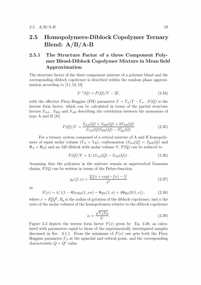
Figure 2.5: (1): 3D-numerical calculations of final configuration of bi-continuous microemulsion at α = 0.1 [55].(2): Transmission electron mi-crography from the symmetric PE/PEP/PE-PEP blend:(a) lamellar,(b)and (c) bicontinuous microemulsion, (d) a two-phase state [19].

The addition of an A-B diblock copolymer to an A/B binary homopolymerblend increases the compatibility between A and B homopolymers. Therefore,those polymer blends are similar to water/oil/surfactant system. A surfactantin oil-water microemulsion stabilizes the interface as the surfactant significantlyreduces the interfacial tension between the oil and water domains. Under someconditions oil, water and surfactant forms a thermodynamically stable structure,known as the microemulsion phase. Microemulsion phases could have the mor-phologies of oil-in-water, water-in-oil, and bicontinuous phases. Oil-in-water andwater-in-oil microemulsion consists of droplets of the minor phase spreaded inthe second one. This type of microemulsion is called droplet microemulsion. Bi-continuous microemulsions are found in systems with approximately equal oiland water composition. The morphology of bicontinuous microemulsions is aspongelike structure.

Depending on the amount of the surfactant Oil-water/surfactant systems ofthe 50/50 water and oil mixture show a two-phase, lamellar-phase, or bicontinu-

2.6. POLYMERIC MICROEMULSION 27

a)

b) c)

A

A-B

B

T

.

1

2A Bφ φ= =

A Bφ −γ

3PL

L

bµE

w in o

o in w 2P2P

2P

T

bµE

Disorder

A HomopolymerB HomopolymerA-B Copolymer

A OilB WaterA-B Surfactant

Figure 2.6: (a): Phase prism for a three-component system. (b): “Fish-cut” isopleth for water-oil microemulsion. (c): “Fish”-cut isopleth for anA/B/A-B polymer blend

ous microemulsion phase. The transition from lamellar to the two-phase regimeoccurs typically between 10% and 30% of the surfactant content.

The complex thermodynamics of symmetric oil/water/surfactant mixturescan be represented by a phase diagram with temperature and concentration of thesurfactant as parameters. The schematic phase diagram of oil/water surfactantmixture and homopolymer/homopolymer/diblock copolymer blend are shown inFig. 2.6(b)-(c).

Recently, in ternary polymer blends A/B/A-B of two homopolymers anddiblock copolymers a channel of bicontinuous microemulsion phase was located[18, 19, 56, 57, 57, 58, 59, 60, 61].

Chapter 3

Experimental

3.1 Sample

3.1.1 Polymer Synthesis and Characterization

All polymers in this study were prepared by anionic polymerization. The tech-niques used were similar to those described by [62, 63]. The homopolymerspolystyrene (PS), deuterated polystyrene (dPS) and deuterated polybutadiene(dPB) were prepared from styrene, deuterated styrene and deuterated butadienemonomers with s-butyllithium as initiator and benzene as polymerization sol-vent. The diblock copolymer dPB-PS and triblock copolymer dPB-PB-dPS weresynthesized by sequential addition of corresponding monomers. The molecularweights and their distributions were determined by size exclusion chromatogra-phy in THF relative to PS-standards. Transformation to the dPB molecularweights was performed by MPB = 0.581M0.997

PS derived from the PS and dPBMark-Houwink-Sekurata relations in THF [64]. The higher molecular weight dueto deuteration was considered during the calculations for the deuterated polybu-tadiene and polystyrene. The molar volume of the homopolymers were relativelysmall and approximately equal: VdPB = 2720cm3/mol, VPS = 2000cm3/moland VdPS = 2065cm3/mol as shown in Tables 3.1 and 3.2. The molar volumeof the symmetric diblock copolymer was chosen approximately six times larger(VdPB−PS = 15400cm3/mol), in order to match the ordering temperatures of thehomopolymer blend and diblock copolymer. The ratio of the molar volumes ofthe homopolymers and copolymer in different contrasts is approximately to beequal α = 0.15 (only in “film” contrast a little bit less α = 0.14). The ratio ofthe two homopolymers was kept constant with the critical value (φPB = 0.42).

29

30 CHAPTER 3. EXPERIMENTAL

Table 3.1: Sample characteristics: Bulk contrast

Sample Polymer Blend Diblock copolymer

Polybutadiene Polystyrene Polybutadiene Polystyrene

93% (1,4) 93% (1,4)Chem. Structure C4D6 C8H8 C4D6 C8H8

dPB PS dPB-PS

Ω[ cm3

mol] 60.6 99.1 60.6 99.1

Density [ gcm3 ] 0.99 1.05

1.025 1.02∑

Nabi

Ωi[1010cm−2] 6.62 1.41 6.62 1.41

Vw[ cm3

mol](Vw

Vn) 2720 (1.05) 2000 (1.06) 15400 (1.05)

N 45 22 137.7 71.5

N 33.6 209.2

PB-composition φ = 0.42 f=0.54

α =√

VPBVPS

VPB−PS0.158

Table 3.2: Sample characteristics: Film contrast

Sample Polymer Blend Triblock copolymer

Polybutadiene Polystyrene Polybutadiene Polybutadiene Polystyrene

93% (1,4) 93% (1,4) 93% (1,4)Chem. Structure C4D6 C8D8 C4D6 C4H6 C8D8

dPB dPS dPB-PB-dPS

Ω[ cm3

mol] 60. 6 100.1 60.6 60.1 100.1

Density [ gcm3 ] 0.99 1.12

1.07 1.05∑

Nabi

Ωi[1010cm−2] 6.62 6.41 6.62 0.41 6.41

Vw[ cm3

mol](Vw

Vn) 2720 (1.05) 2065 (1.06) 17200 (1.05)

N 45 22 135 16 81

N 33.6 232

PB-composition φ = 0.42 0.47 0.06 0.47

α =√

VPBVPS

VPB−PS0.140

3.1. SAMPLE 31

Table 3.3: Investigated samples

“Bulk” “Film” “Block” CharacteristicAlias Volume Alias Volume Alias Volume

Fraction Fraction Fraction

B00 0.000 F00 0.000 F00 0.000B03 0.030 F03 0.030 C03 0.030 Disorder-B04 0.040 - - - - Two-PhaseB05 0.050 F05 0.050 - - TransitionB06 0.060 F06 0.060 - -

B066 0.066 - - C065 0.065 Disorder-B07 0.070 F07 0.070 - - Two-Phase-B071 0.071 - - - - MicroemulsionB072 0.072 - - - - Transition

B073 0.073 - - C074 0.074B075 0.075 - - - -B08 0.080 F08 0.080 C08 0.079 Disorder-B09 0.090 - - - - MicroemulsionB10 0.100 F10 0.100 C10 0.100 Transition

B13 0.131 - - - -B15 0.150 F15 0.150 - - Disorder-B20 0.200 - - - - LamellarB30 0.300 - - C30 0.302 TransitionB40 0.400 - - - -B50 0.500 - - - -B100 1.000 F100 1.000 B100 1.000

3.1.2 Sample Preparation

A preparation of a blend consisting of two immiscible homopolymers at roomtemperature differs from mixing of simple liquids. Due to the high viscosity andthe temperature range of experiment (20-160C) there was not possible to useconventional quartz cells. The cells are shown in Fig. 3.1.

The preparation of polymer blends for SANS was done by the freeze-driedmethod. First, the two polymer blends of dPB/PS and dPB/dPS with identicalvolume fraction of deuterated Polybutadiene φ = 0.42 were prepared. The volumefraction of the final sample was determined by recalculating the weight of thecomponents considering the density of the homopolymers depicted in Tables 3.1and 3.2. At room temperature the PB/PS blend is immiscible. In order toget a macroscopically homogeneous blend the follows procedure was exploited.


The homopolymers were dissolved in benzene followed by two hours of shakingand quickly freezed to a temperature of approximately −10... − 5C. At thistemperature benzene is in solid state. The frozen mixture was then set up to avacuum line. In order to avoid a distribution of the material inside of vacuum linethe sublimation of benzene was done step by step by opening and closing the valveof the vacuum line. During the first few minutes more than 95% of the solvent wassublimated. The samples were dried under vacuum conditions during 24 hours atleast. Ternary polymer blends in bulk, film and block contrast conditions wereprepared by the above mentioned method by mixing the homopolymer blendand the diblock (triblock) copolymers. The parameters of the explored samplesare listed in Table 3.3. After preparation the blends were closed in an argonatmosphere and kept in the refrigerator.

Figure 3.1: Cell for SANS

The next step of the sample preparation was to transfer the sample to theSANS cell. The cells were filled in a glove box under argon atmosphere at atemperature slightly above of the melting temperature.

3.1.3 Thermostat

Near the critical point a small change of temperature induces a large and non-linear change of the degree of thermal fluctuations. Therefore, investigations ofcritical phenomena require a precise and stabile temperature. An oven with a

3.1. SAMPLE 33

two-level temperature control was used [65]. The “real” temperature of samplewas corrected to temperatures of inner Tinside and tube Ttube parts of the oven as

Tsample[C] = Tinside − 0.060 (Tinside − Ttube)

2 − 5.45.10−4 (Tinside − Ttube) (3.1)

in order to take into account temperature gradient effects inside the thermostat.The temperatures were measured by a 10Ohm platinum resistance element. Twolevel temperature heating devices in conjunction with the vacuum chamber al-lowed to keep the temperature of a sample as long as it is necessary with atemperature stability better than 0.02K.


3.2 Small Angle Neutron Scattering

The scattering measurements were performed at the KWS1 and KWS2 diffrac-tometers at the FRJ-2 research reactor of the Forschungszentrum Julich (FZJ)[66]. The characteristics of both diffractometers and the experimental conditionsare shown in Table 3.4.

Table 3.4: Instruments details

Characteristic KWS1 KWS2

Monochromator Velocity selector [DORNIER] Velocity selector∆λ/λ 0.2 0.1Wavelength,λ 7A 7ASample aperture, ds 0.7 cm 0.9 cmCollimation aperture, 3 × 3 cm 3 × 3 cmCollimation length 2 - 20m 2-20mDetector length 1.25 - 20m 1.4-20mDetector:

Active area 60 × 60 cm2 50 × 50 cm2

Scintillator 6Li − Glas 3HeSpace resolution 8mm 8mmMax.pulse rate 12.5 kHz 7 kHzDead time, τd 8.8µs 15µs

Q-range 2.10−3 − 0.2 A 2.10−3 − 0.2 ANeutron flux at sample 2.105 − 2.107 n/cm2s 105 − 6.106 n/cm2s

3.2.1 Basics of Small Angle Neutron Scattering

The experimental setup and the geometry of a scattering experiment of the smallangle scattering instrument is schematically depicted in Fig. 6.2. An importantadvantage of the neutrons is their deep penetration into samples due to theirweak interaction with atomic nuclei.

The scattering vector is defined as the difference between the propagationvectors of the scattered and incident beam ( Fig. 6.2)

~Q = ~k − ~k0 (3.2)

In case of elastic small-angle scattering the energy transfer is neglected (|~k| = |~k0|)and the scattering intensity is discussed in terms of momentum transfer Q given

3.2. SMALL ANGLE NEUTRON SCATTERING 35

1-20m

θ

1-20m

Selektor Collimation

SampleAppertures

Detektor tube Detektor

ko

k1

Figure 3.2: General layout of a scattering experiment

as

Q =4π

λsin

Θ

2, (3.3)

where λ is the wavelength of neutrons adjusted by the frequency of the velocity se-lector. The macroscopic cross-section dΣ/dΩ(Q) is connected with the scatteringintensity ∆I(Q) in solid space angle ∆Ω and given by the equation

dΣ

dΩ(Q) =

1

εVpTI0

∆I(Q)

∆Ω, (3.4)

with the scattering sample volume Vp, the transmission T , the incoming neutronintensity I0, and the efficiency of the detector channels ε. In polymer blends thescattering cross-section can be expressed in terms of the structure factor S(Q) as

dΣ

dΩ(Q) = K .S(Q), (3.5)

with the contrast factor K given by

K =(∆ρ)2

NA

, (3.6)

with scattering contrast (∆ρ)2 and the Avogadro number NA. The scatteringcontrast of i and j polymers is calculated as the function of the molar monomervolume Ωi and the coherent scattering length bi

(∆ρ)2 = N2A

(∑

i bi

Ωi−∑

j bj

Ωj

)2

. (3.7)

The coherent lengths of a few isotopes are listed at Table 3.5. The huge differencebetween 1H and 2D in the coherent scattering length is the basis of contrast


variation and the matching technique. An isotopical substitution does not changethe physical and chemical properties of the mixture in most cases, but cruciallychanges the scattering properties of the system. In Table 3.6 the scatteringcontrast (∆ρ)2 and the contrast factor K are shown for the investigated polymers.

Before the data interpretation the incoherent scattering has to be sub-tracted:

dΣ

dΩ

∣

∣

∣

∣

coherent

=dΣ

dΩ

∣

∣

∣

∣

measured

− dΣ

dΩ

∣

∣

∣

∣

incoherent

. (3.8)

The incoherent scattering of polymer given by

dΣ

dΩ

∣

∣

∣

∣

incoherent

=1

4π·∑

i σinci

Ωi. (3.9)

The incoherent scattering lengths σinci of are listed at Table 3.5. The strongest

incoherent scattering comes from hydrogen. Table 3.7 contents the incoherentstructure factor for several systems.

3.2.2 Raw Data Reduction

The scattering patterns were corrected in a standard way by detector sensitivity,background, and is given in absolute units after being calibrated by a Lupolensecondary standard.

The scattering intensity is related to cross section by

∆I(Q) = I0 ε ∆Ω A d TdΣ

dΩ(Q)

where A is illuminated area, d the sample thickness. By using Lupolen as a sec-ondary standard with the scattering intensity ILupolen the intensity of the sampleISample could be rewritten in terms of the scattering cross-section

ISample

ILupolen=

∆ΩSample

∆ΩLupolen· dSample

dLupolen· TSample

TLupolen·

dΣ/dΩ|Sample

dΣ/dΩ|Lupolen

. (3.10)

Reorganizing of Eq. 3.10 using the definition of solid space angle ∆Ω ∼ 1/L2

with the sample-detector distance L, the scattering cross-section of sample followsnext equation

dΣ

dΩ(Q) = cal · ISample (3.11)

where constant cal is given by

cal =L2

Sample

L2Lupolen

· dLupolen

dSample

· TLupolen

TSample

·dΣ/dΩ|Lupolen

< ILupolen >. (3.12)

Addition measurements of scattering from empty cell Icell, blocked beam IBG wascarried out. The final scattering cross-section becomes

dΣ

dΩ(Q) =

ISample − IBG − TSample/TEmpty(IEmpty − IBG)

ILupolen − IBG − TLupolen/TEmpty(IEmpty − IBG)· cal. (3.13)


Table 3.5: The coherent and incoherent scattering lengths of some iso-topes

Isotope 1H 2D Cb [10−12cm] −0.3740 +0.6674 +0.6648

σinc [10−24cm2] 80.2 2.05 < 0.018

Table 3.6: Contrast factor

System (∆ρ)2 [10−20cm−4] K = NA/(∆ρ)2[cm4/mol]

dPB/dPS 0.043 1.41 · 105

dPB/PS 27.0 222.2dPB/PB 38.5 156.6PB/dPS 36.0 167.4

Table 3.7: Incoherent background

System dΣdΩ

∣

∣

inc[cm−1] Sinc[cm

3/mol]

dPB/PS 0.184 40.97dPB − PS 0.148 32.90dPB/dPS 0.0087 1220

dPB − PB − PS 0.0276 4.47

3.2.3 Dead Time Effect

Local sensitive detectors of SANS instruments have a characteristic time for de-tection a single event. This finite time of detector can lead to dead-time effectswith a characteristic time τd. This time gives a characteristic restriction, whichhas to be taken into account specially at high counting rates. Within the dead-time counts are lost. The reasons for this restriction are the electronic deviselimitations and data acquisition electronics. The scattering profile could be cor-rected with respect to dead-time effects as given by

dΣ

dΩ(Q0)

∣

∣

∣

∣

corrected

=dΣdΩ

(Q0)

1 − τdNtot

. (3.14)

Dead-times of KWS1 and KWS2 diffractometers are 8.8µs and 15µs, respectively.The dead-time correction was applied for samples that scatter strongly in high-Qrange.


3.2.4 Resolution Function

l

L

R

r

α1

α2

Detector SampleAperture

CollimationAperture

Sample

Figure 3.3: Aperture configuration

The observed scattering intensity is smeared by the distribution of the wave-length, a finite beam divergence, and the finite channel size of a detector.

The experimentally measured intensity I(Q) and the scattering cross sectiondΣ/dΩ(Q0) as a function of the average scattering vector Q0 are connected as[67, 68, 69]

I(Q) =

∞∫

0

R(Q, Q0)dΣ

dΩ(Q0)dQ0 (3.15)

where R(Q, Q0) is the resolution function. Pedersen et al. [67, 68, 69] approxi-mated the resolution function by Gaussian functions given as

R(Q, Q0) =1

σQ

√2π

exp

(

−(Q − Q0)2

2σ2Q

)

(3.16)

with the dispersion coefficient σQ. The smearing effects are mainly caused bywavelength spread ∆λ (the velocity selector), collimation effects (the finite beamdivergence), and detector resolution (the discretivity of the defector). These threeeffects are included in the dispersion coefficient as

σ2Q =

1

8 ln 2

[

Q20

(

∆λ

λ

)2

+ k20 (∆Θ)2 + k2

0

(

D

l

)

]

, (3.17)


with k0 = 2π/λ, and ∆λ being the full-width at half-maximum of wavelengthspread, D the size of the detector channel, l the detector-to-sample distance.The second term in Eq. 3.17 takes the collimation effect into account. Theconfiguration of the apertures is shown at Fig. 3.3. The ∆Θ vs. the geometricalparameters of the experiment L (the sample aperture - detector distance), r (theradius of the sample aperture), R (the radius of the collimation apertures) areexpressed as [68, 69]

∆Θ =

2RL

− r2

2R(l+L)2

l2L, α1 ≤ α2

2r(

1l+ 1

L

)

− r2

2Rl

L(l+L), α1 > α2

. (3.18)

The experimental data were fitted by a model considering the resolutionfunction.

Chapter 4

Experimental results

4.1 Phase Diagram

The temperature-diblock concentration plane of the phase diagram of the ternarydPB/PS/dPB-PS mixture with fixed critical concentration of the dPB/PS blendhas been depicted in the range from 0 to 20% in Fig.4.1. This phase diagramrepresents the principle results of this work and is therefore a reference for thepresentation of the experimental data. The depicted boundaries will be discussedin the following.

The phase diagram in Fig.4.1 is globally divided by the Lifshitz line into twocharacteristically different parts with respect to the behavior of the system. Onthe left from the LL in the disordered phase at higher temperature the ternarysystem demonstrates a so-called “blend”-like behavior of the structure factor withthe maxim an intensity at Q = 0. On the right side from the Lifshitz line themaximum of the intensity is observed at a finite Q∗ value and the behavior of themixture is called ”diblock copolymer“-like one. At high temperature randomlydistributed diblock copolymers modulate the homopolymers.

4.1.1 Lifshitz Line

The mean field theory predicts the Lifshitz line at a constant concentration deter-mined from the ratio of the molar volumes α = 0.158 and is accordingly estimatedwith 4.7% Eq. 2.40 for the present system.

The Lifshitz line in Fig. 4.1, however, shows characteristic deviations. Athigh and low temperatures it is observed at the larger diblock concentration of7%, in comparison with the mean field prediction of 4.7%, and it bends to evenlarger concentrations at intermediate temperatures near the two-phase regime.Such bending is caused by thermal composition fluctuations as has been shownfrom recent renormalization group theory calculations [32].

The Lifshitz line was detected by an isothermic and isopleth approach. InFig. 4.2 the concentration dependence of Q∗ is shown for three temperatures.

41

42 CHAPTER 4. EXPERIMENTAL RESULTS

0 2 4 6 8 10 12 14 16 18 2020

40

60

80

100

120

140

160

Disordered"Homopolymer" Disordered

"Diblock Copolymer"

Lamella

DµE

Lifshitz Line

BµE

Two-Phase

Tem

pera

ture

[°C

]


Double Critical Point"Multiple" Critical Point

Figure 4.1: Experimental phase diagram of the dPB/PS/dPB-PS blend.The filled circles (•) represent the upper and lower critical temperaturesof the 3D-Ising and isotropic Lifshitz case separated by grey box, the opencircle () the double critical point, the filled stars (

) the disordered

Lifshitz line, the open stars () the microemulsion Lifshitz line, the filledtriangle () the disorder-microemulsion boundary, the diamonds () thedisorder-order (lamellar) transition, () the disorder line. The dashedarea separates the lamellar phase and bicontinuous microemulsion

Already at 50C and the other temperatures a visual distinction can be made forthe scaling behavior of Q∗. From an analysis of a concentration scaling behaviorQ∗ ∼ |Φ−ΦLL|βQ two parameters were determined for each temperature, namelythe LL position ΦLL and the exponent βQ. This analysis was performed in atemperature range from 25 to 160C. There is a clear difference in the behaviorof the exponent βQ below and above 71C as depicted in Fig. 4.3. Two exponentsof βQ = 0.3 and βQ = 0.42 were observed above and below 71C, respectively.These two exponents are due to the different nature of the LL in the disorderedand ordered regimes of the phase diagram. In the sections of 5.3 and 4.1.3 theevidence of a disorder-microemulsion boundary is represented. This boundaryis shown by the filled triangles in Fig. 4.1. The LL crosses the microemulsionboundary exactly at 71C where we detected the abrupt change of the scalingbehavior of the Q∗ position. We call the LL at high temperatures the “disordered”Lifshitz line (dLL), at low temperatures in an ordered part of phase diagram the

4.1. PHASE DIAGRAM 43

5 10 15 20 25 30 350.00

0.01

0.02

0.03

0.04

Q*~|Φ-Φo|βQ

T=120oC, β=0.3

T=70oC β=0.3

T=50oC β=0.42

Q* [Å

-1]


Figure 4.2: Concentration scaling of the peak position Q∗ ∼ |Q−QLL|βQ

near the disordered Lifshitz line at 120oC (•), near the microemulsionLifshitz line at 50oC (), and near “intersection” of dLL and µLL at70oC ()

20 40 60 80 100 120 140 160

0.25

0.30

0.35

0.40

0.45

<βQ>=0.30

<βQ>=0.42

Exp

one

nt β

Q

Temperature [°C]

TLC

=71.1°C

Figure 4.3: The concentration dependence of the βQ exponent.


40 60 80 100 120 140 1600.0

0.5

1.0

1.5 dPB/[email protected]%dPB-PS (B7.3%)

Q*=2.2 10-3|T-TLL

|0.4

Q*[

10-2Å

-1]

T[°C]

TµLL

=60.6°C

Figure 4.4: The temperature dependence of Q∗-value near the LL: the7.3% sample

40 60 80 100 120 140 1600.0

0.5

1.0

1.5 dPB/[email protected]%dPB-PS (B7.5%)

Q*=1.9 10-3|T-TLL

|0.4

Q*[

10-2Å

-1]

T[°C]

Q*=4.1 10-3|T-TLL

|0.31

TdLL

=94.6°C

TµLL

=65.6°C

Figure 4.5: The temperature dependence of Q∗-value near the LL: the7.5% sample


40 60 80 100 120 140 1600.0

0.5

1.0

1.5 dPB/PS@8%dPB-PS (B8%)

Q*=2.22 10-3|T-TLL

|0.4

Q*[

10-2Å

-1]

T[°C]

Q*=3.0 10-3|T-TLL

|0.4

TdLL

=90.7°C

TµLL

=67.8C

Figure 4.6: The temperature dependence of Q∗-value near the LL: the8% sample

40 60 80 100 120 140 1600.0

0.5

1.0

1.5

2.0 dPB/PS@9%dPB-PS (B9%)

Q*=3.7 10-3|T-TLL

|0.3

Q*[

10-2Å

-1]

T[°C]

Q*=4.9 10-3|T-TLL

|0.3

TµΕ

=70°C

Figure 4.7: The temperature dependence of Q∗-value near the LL: the9% sample


“microemulsion” Lifshitz line accordingly to (µLL), while the total line accordingto LL.

In the disordered phase the appearance of the peak above the dLL is mainlycaused by the diblock-diblock structure factor. On the other hand the µLL is theresult of cooperative phenomena and represents a transition from a droplet to abicontinuous microemulsion phase. So, the µLL is caused by the disappearanceof the correlation between the microemulsion particles. We already mentionedhere that the depicted line does not separate correlated droplets (dµE) but abicontinuous microemulsion phase. This will be discussed later in more detailand could only be concluded from measuring samples with different scatteringcontrasts.

In Fig. 4.9(b) the temperature dependence of the peak position is plottedvs. temperature in block and film contrasts. In both contrasts the Lifshitzlines are located at the same temperatures. The point of intersection of the twoLifshitz lines is a special point of the phase diagram, where two disordered andtwo microemulsion phases coexist.

According to Brasovskii [70] the transition from a disordered to the lamellarphase is predicted to be first order therefore it is a discontinuous one.

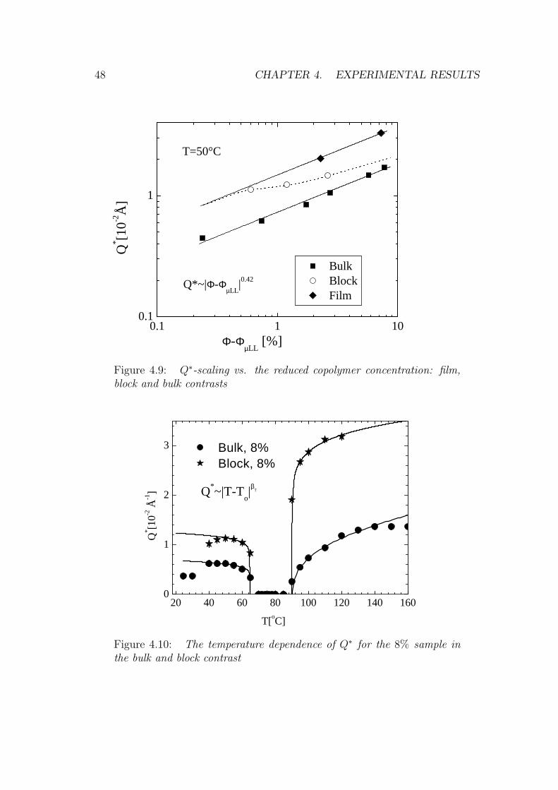
The temperature dependence of the Q∗-values near the LL samples 7.3%,7.5%, 8% and 9% is shown in Figures 4.4-4.7. At the Lifshitz temperature Q∗

becomes 0. The behavior of Q∗ near the Lifshitz line can approximately be de-scribed by a scaling law Q∗ ∼ |T −TLL|βT with an exponent βT being 0.4 and 0.3when approaching TLL from microemulsion and disordered phases, respectively.The MF approximation predicts a scaling behavior of the peak position vs. tem-perature in the vicinity of the Lifshitz line with an exponent of 0.4 [18]. Thechange of Q∗ with Φ has been plotted in Fig. 2.4(b), it does not follow simplescaling law over the whole diblock concentration regime. Only near the Lifshitzline a power law behavior with an exponent between 0.3 and 0.4 is predicteddepending on the chosen fitting range of the scaling law.

4.1.2 Disorder Line

As mentioned in Chapter 2 the correlation function shows damping oscillationson the right side of the disorder line. From an experimental point of view this linecan be detected by SANS. Approaching to DL from the “diblock”-like part of thephase diagram the periodicity length in the system increases, which thus leads todecrease of the maximum position of the scattering profile. The mean field defi-nition of the disorder line is expressed by the structure factor parameters S−1(0),L2 and L4; exactly at the disorder line the parameter λTS becomes infinite. TheDL was determined from the temperature and concentration dependence of λTS.In Fig. 4.8 the temperature dependence of λTS is shown for the 6.6% sample.

A more clear physical meaning of the disorder line can be obtained fromthe correlations length ξL2

and ξL4. At the disorder line both correlation length


60 80 100 120 14010

100

1000

Tc

DL

dPB/[email protected]%dPB-PS

λTS

ξTS

ξQ

2

ξQ

4

Len

gth[

Å]

T[°C]

Figure 4.8: The temperature dependence of the different length scaleparameters λTS, ξTS, ξL2

and ξL4of the sample with φ = 6.6% diblock

content. Dashed lines limit the two-phase range. Lines are the disorderlines of this sample

becomes equal. In Fig. 4.8 the correlation lengths ξL2and ξL4

are plotted togetherwith other relevant length scales λTS and ξTS.

Due to the vanishing of the Q2-term of the inverse structure factor S−1(Q) atLL, two correlation lengths, namely ξQ2 and ξQ4, have to be considered. Below 5%the ξQ2 correlation length dominates in the whole temperature range, ξQ2 ξQ4,and the structure factor follows the Ornstein-Zernike approximation. Above 5%diblock content at high temperatures, ξQ4, dominates. In decreasing temperaturethe system crosses the disorder line, where the oscillations of the correlationfunction vanish. At the DL the two correlation lengths become equal, and belowthe DL thermal fluctuations are ordered by the diblock copolymer. Below DLthermal fluctuations rearrange the diblock copolymers by accumulating them attheir interface.

4.1.3 Microemulsion Phases

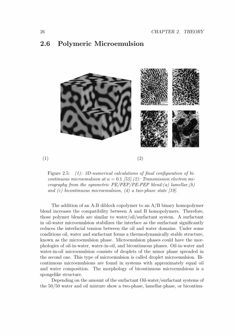
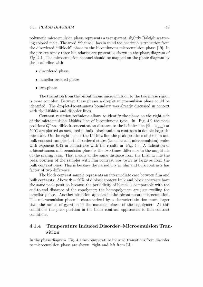
A microemulsion channel was detected between the two-phase and lamellar or-dered phase in the dPB/PS/dPB-PS system between Φ = 6% and 13%. The


0.1 1 100.1

1

T=50°C

Bulk Block Film

Q* [1

0-2Å

]

Φ-ΦµLL

[%]

Q*~|Φ-ΦµLL

|0.42

Figure 4.9: Q∗-scaling vs. the reduced copolymer concentration: film,block and bulk contrasts

20 40 60 80 100 120 140 1600

1

2

3

Q*~|T-To|βΤ

Bulk, 8% Block, 8%

Q* [1

0-2 Å

-1]

T[oC]

Figure 4.10: The temperature dependence of Q∗ for the 8% sample inthe bulk and block contrast


polymeric microemulsion phase represents a transparent, slightly Raleigh scatter-ing colored melt. The word “channel” has in mind the continuous transition fromthe disordered “diblock” phase to the bicontinuous microemulsion phase [19]. Inthe present study three boundaries are present as shown in the phase diagram ofFig. 4.1. The microemulsion channel should be mapped on the phase diagram bythe borderline with

disordered phase

lamellar ordered phase

two-phase.

The transition from the bicontinuous microemulsion to the two phase regionis more complex. Between these phases a droplet microemulsion phase could beidentified. The droplet-bicontinuous boundary was already discussed in contextwith the Lifshitz and disorder lines.

Contrast variation technique allows to identify the phase on the right sideof the microemulsion Lifshitz line of bicontinuous type. In Fig. 4.9 the peakpositions Q∗ vs. diblock concentration distance to the Lifshitz line (Φ−ΦµLL) at50C are plotted as measured in bulk, block and film contrasts in double logarith-mic scale. On the right side of the Lifshitz line the peak positions of the film andbulk contrast samples in their ordered states (lamellar and microemulsion) scaleswith exponent 0.42 in consistence with the results in Fig. 4.3. A indication ofa bicontinuous microemulsion phase is the two times difference in the amplitudeof the scaling laws. That means at the same distance from the Lifshitz line thepeak position of the samples with film contrast was twice as large as from thebulk contrast ones. This is because the periodicity in film and bulk contrasts hasfactor of two difference.

The block contrast sample represents an intermediate case between film andbulk contrasts. Above Φ = 20% of diblock content bulk and block contrasts havethe same peak position because the periodicity of blends is comparable with theend-to-end distance of the copolymer; the homopolymers are just swelling thelamellar phase. Another situation appears in the bicontinuous microemulsion.The microemulsion phase is characterized by a characteristic size much largerthan the radius of gyration of the matched blocks of the copolymer. At thisconditions the peak position in the block contrast approaches to film contrastconditions.

4.1.4 Temperature Induced Disorder–Microemulsion Tran-

sition

In the phase diagram Fig. 4.1 two temperature induced transitions from disorderto microemulsion phase are shown: right and left from LL.


10-3 10-2103

104

105

106

DisorderedPhase

T=31.41oC

T=45.94oC

T=55.49oC

T=64.94oC

T=75.00oC

T=85.00oC

T=95.00oC

T=120.00oC

T=150.00oC

dPB/PS@9%dPB-PS (B09)S(

Q)[

cm3 /m

ol]

Q[Å-1]

MicroemulsionPhase

Figure 4.11: B09%: Temperature induced bicontinuous microemulsionformation. The lines represent fits accordingly to Eq. 2.3


10-6

10-5

10-4

0.8

1.2

1.6

101

102

103

2.4 2.6 2.8 3.0 3.20.0

0.4

0.8

S-1(0)

S-1(Q*)

dPB/PS@9%dPB-PS (B09)

S-1(0

;Q* )[

cm3 /m

ol]

(1)

(2)

Q* [1

0-2Å

-1]

(3)

ξTS

λTS

/(2π)

ξQ4 le

ngth

[Å]

(4) D

m

1/T[10-3/K]

Disorder-microemulsion boundary

Figure 4.12: B09%: Temperature induced bicontinuous microemulsionformation. The temperature dependence of the parameters: (1):the sus-ceptibilities S−1(0) and S−1(Q∗),(2): the peak position Q∗; (3) the TS-periodicity λTS, the TS-correlation length ξTS, the Q4-correlation lengthξQ4; (4) the disorder parameter Dm


On the left side from the Lifshitz line a transition from the disordered stateto the droplet microemulsion phase is shown by the filled triangles. The structurefactors measured above and below this borderline have their maximum at Q = 0.This line is plotted at temperatures, where the susceptibility has a maximumvalue as shown in Section 5.3.

On the right side of the LL, in the diblock-like part of the phase diagramthe disorder-bicontinuous microemulsion boundary is plotted at a position wherethe structure factor changes its behavior. In Fig. 4.11 the structure factors of theternary blend with 9% diblock content are shown for several temperatures. Thestructure factors were fitted by Eq. 2.3 taking into account resolution effects asdescribed above in theory section. Parameters of the fit, namely the susceptibility(S(0) and S(Q∗)), the peak position (Q∗), the length scales (ξQ4, ξTS, λTS) andthe disorder parameter Dm, are depicted at the Fig. 4.12(1-4). Plotted propertiesshows a different behavior in disordered and bicontinuous microemulsion phasesseparated by the line in Fig. 4.12.

The susceptibility S(Q∗) continuously changes from disordered to microemul-sion phase in contrast to S(0). Above and below T = 69oC the “0-susceptibility”shows a distinguished temperature behavior.

The peak position has a different nature above and below the microemul-sion borderline. Above the disorder-microemulsion boundary the existence ofa peak in the structure factor is caused by the diblock-diblock structure fac-tor. Below the microemulsion boundary diblock copolymers are distributed onthe homopolymer-homopolymer interface. In microemulsion phase the peak ofthe scattering curve is caused by an alternative distribution of PB- and PS-homopolymer.

The correlation function ξQ4 demonstrates two different behavior at highand low temperature. The Teubner-Strey and “Q4”-correlation length have thesame temperature behavior, as one can see in Fig. 4.12(3). In disordered phasethe decreasing of the temperature increases the correlation length. Bicontin-uous microemulsion phase is characterized by an approximately temperature-independent correlation length.

4.1.5 Lamellar - Bicontinuous Microemulsion Transition

Between Φ = 10% and 13% we identified the boundary between the lamellarordered phase and the bicontinuous microemulsion phase. This transition has afirst order nature. From the SANS measurements the susceptibility S−1(Q∗) andthe peak position Q∗ change continuously from lamellar phase to bicontinuousmicroemulsion phase. The peak positions Q∗ in different contrasts at 50C areshown in Fig. 4.9 and no indication of the transition is visible. The distinction ofthe ordered lamellar phase is the appearance of a second order peak and a jumpof the susceptibility indicating a first order disorder-order boundary. Clearly, onecan see in the Fig. 4.13 the second order peak at Q∗ = 2Q∗ for 13% of the diblock


content and no second order peak for 10%.

4.1.6 Order-Disorder Transition of the Diblock Copoly-mer melt

The order-disorder transition of the symmetric copolymer dPB-PS melt was alsostudied in “bulk” and “block” contrast. The characteristics of the diblock copoly-mers are listed in Table 3.1. The diblock copolymer melt dPB-PS with a molec-ular volume 15400cm3/mol has already been under investigation in early stud-ies [71,72]. There the temperature dependence of the scattering profile was mea-sured at different pressure field and solvent [73]. In Fig. 4.15 the temperaturedependence of the structure factor, the susceptibility and peak position of thisdiblock copolymer are shown. The copolymer melt has a disorder-order transi-tion at 69.4C. As the diblock copolymers is symmetrical the ordered phase hasa lamellar structure.

A melt with triblock copolymers dPB-PB-dPB was also measured and wasused for film contrast measurements.The protonated PB-part of the triblockcopolymers occupies roughly 6% of the copolymer volume. The structure fac-tor of triblock copolymers is discussed in Sec. 4.3 and their peak positions vs.temperature are displayed in Fig. 4.15 together with the peak position of the di-block copolymer dPB-PS. With temperature an overall increase of Q∗ is observedindicating a chain stretching with decreasing temperature.

A clear disorder-order transition is visible from a sudden change of Q∗ forthe sample undo film contrast. At the TODT the copolymer appears slightlyrelaxed by the ordering process. This decrease of length could also be a result ofthe ordering and not from the chain itself, this effect is not visible in the “bulk”melt.

The periodicity of the ordering to the lamellar phase appears in two respectsdifferent in bulk and film contrast. The peak position Q∗ of the structure functionof the triblock copolymer melt dPB-PB-dPS should be twice as large as in thedPB-PS case of equal molecular volumes. In Fig. 4.15 by stars are depictedtwice as larger Q∗ of diblock copolymer melt dPB-PS corrected to difference ofmolecular volumes between diblock and triblock copolymers.

In the ordered phase a factor of two difference for the peak positions forbulk and film contrast is evident.

4.1.7 Ordering Transition in A/B/A-B Blend

The analysis of the structure factor S(Q) measuring thermal composition fluctua-tions in the disordered state of the three component polymer mixture was mainlyperformed on the basis of the formalism developed by Kielhorn and Muthuku-mar [74]. This theory takes the effects of thermal fluctuations into consideration,


10-3 10-2 10-1

101

102

103

104

2Q*

10% BµE 13% Lamellar

T=40oC

d Σ/d

Ω [

cm-1]

Q[Å -1]

Q*

Figure 4.13: The scattering profile of the 10% and 13% samples, in thebicontinuous and lamellar phase, respectively, at T = 40C

10-3 10-2 10-1100

101

102

103

104

105

6.5% 7.5% 8% 9% 10% 13% 20% 30% 40% 50%

T=40oC

d Σ/d

Ω [

cm-1]

Q[Å -1]

Q-4

Figure 4.14: The scattering profiles at T = 40C: two-phase, droplet,bicontinuous, lamellar phases


20 40 60 80 100 120 140 1600

2

4

6

8

10TdPB-PS

ODT=69.4°C

Q* [1

0-2Å

-1]

T[oC]

TdPB-PB-dPS

ODT=90.4°C

dPB-PB-dPS dPB-PS

2QBulk/VFilm

w*VBulk

w

Figure 4.15: The position of the maximum intensity Q∗ vs. tempera-ture: dPB-PS() and dPB-PB-dPS (?), the filled circles (•) being thetwice large position of maximum of diblock copolymer () corrected tothe different volume of diblock and triblock copolymers.

as was reviewed in the theoretical part. For samples with diblock concentrationslarger than the Lifshitz line with the maximum of S(Q) occurring at a finite Q,the most general application started with the analysis of S(Q) by Eq. 2.44 (seesolid lines in Fig. 4.16), which for each equilibrium state delivers four param-eters, namely, a, b, c, d. Based on these four values and their expressions, theFH-parameter, the Ginzburg parameter, and the statistical segment length werecalculated for each temperature. The obtained FH-parameter has been listed inTable 5.2.

4.1.8 Phase Diagram in Different Contrasts

In order to better understand the role of diblock copolymers in a binary melt ofhomopolymers the contrast variation method was used. Most of the investigationsof the ternary blend PB/PS/PB-PS were carried out in “bulk”-contrast using thedPB/PS/dPB-PS blend, when the fluctuations of only one polymer componentwere made visible to SANS.


0 2 4 6 81

10

100

dPB/PB@50%dPB-PS T[°C]

T=149.2oC

T=140.8oC

T=132.3oC

T=123.7oC

T=114.9oC

T=106.1oC

T=92.6oC

T=83.5oC

T=78.9oC

T=69.6oC

T=60.2oC

T=53.1oC

T=50.7oC

T=43.5oC

T=36.3oC

T=29.4oC

d Σ/d

Ω[c

m-1]

Q[10-2Å-1]

Figure 4.16: The scattering profile of the 50% sample at different temperatures.The solid lines represents a fit of the structure factor by Eq. 2.44

2.4 2.6 2.8 3.0 3.20

1

2

3

4

5

2.9 3.0 3.1 3.2 3.30.0

0.2

0.4

0.6

0.8

dPB/PS@50%dPB-PS

S-1(Q

*)[1

0-4m

ol/c

m3 ]

1/T[10-3/K]

TODT

=45°C

2.4 2.6 2.8 3.0 3.23.0

3.2

3.4

3.6

3.8

4.0

TODT

=45°C

dPB/PS@50%dPB-PS

Q*[

10-2Å

-1]

1/T[10-3/K]

(a) (b)

Figure 4.17: The susceptibility S−1(Q∗) and the peak position Q∗ vs. inversetemperature 1/T


0 5 10 50 100

50

100

150 film contrast bulk contrast

"Blend-like"region

"Diblock-like"region

Ordered phase (Lamella)

MicroEmulsionchannel

Two-Phase

Tem

pera

ture

[°C

]


Figure 4.18: Phase diagram: the bulk (solid lines) and film contrast(dashed lines)

The scattering length density of investigated polymers are listed in Ta-bles 3.1 and 3.2. Deuterated polybutadiene and deuterated polystyrene haveapproximately the same scattering length density, thus in the ternary system ofdPB/dPS/dPB-PS only the polystyrene block of the diblock copolymers is visi-ble. Isotopical exchange has some influence on the Flory-Huggins parameter andleads to a shift of the phase transition as well as critical temperature. A similarsituation is met for isotopical exchange of diblock copolymers.

In addition a slightly different chain length can also have some influenceon the phase transition line. In Fig. 4.18 for comparison the phase boundariesof the PB/PS/PB-PS blends in “bulk” and “film” contrasts are depicted. The”film” contrast samples always shows a phase transition lines between 10 and20K above “bulk”. In the limiting cases of Φ = 0 and Φ = 1 the exchange of thehomopolymer and diblock copolymers is the responsible one, respectively.

Due to the vanishing scattering contrast between dPB and dPS we werenot able to measure the critical solution point by SANS. Instead the cloud pointsbelow the Lifshitz line were determined by turbidity measurements. This methodof determination of the critical temperature is not so precise as SANS, but allowsa sufficient precise estimation of Tc. In both blends the components dPS and PShave an approximately identical molecular volume. Therefore, the shifting of thecritical temperature is mainly caused by a variation of the FH parameter due to


the exchange of deuteration.With the increase of diblock copolymer content the differences between the

critical temperatures of bulk and film contrast samples are reducing and themicroemulsion channel seems not to be affected from reasons we presently do notunderstand.

The phase boundaries of the “block” contrast sample is not plotted in thisgraph. But for obvious reasons, their line of critical points follows the same one asthe “film” contrast one, as the homopolymer blend is identical, while the order-disorder borderline follows the bulk contrast sample, since the diblock copolymerwas not changed.

4.2. CRITICAL EXPONENTS AND CROSSOVER 59

4.2 Critical Exponents and Crossover

In this section the behavior of thermal composition fluctuations in the disorderedregime below the Lifshitz line is discussed in terms of critical exponents of the sus-ceptibility and the corresponding correlation length as obtained from asymptoticscaling laws.

4.2.1 Ising Critical Behavior

Below Φ = 5% the critical behavior of the investigated ternary blend behaves sim-ilarly to binary homopolymer blends. The structure factor of thermal fluctuationsfollows to the Ornstein-Zernike approximation. In Fig. 4.19(a-c) the structurefactor of three samples with diblock content less 5% are plotted for several tem-peratures in the Zimm representation S−1(Q) vs. Q2. In the range of small Q theinverse structure factor S−1(Q) is fitted by a line in Zimm representation. BelowΦ = 5%, the 0%, 3% and 4% samples were fitted by the OZ-equation with thesusceptibility S−1(0) and the correlation length ξQ2 as adjustable parameters.

At the binodal temperature the susceptibility S(0) has a maximum. Thespinodal temperature can be determined by the approximation of the inversesusceptibility by a scaling law to an infinite value. At the critical point (criticalconcentration) the binodal and spinodal temperatures are equal.

One can see from Fig. 4.22(a) the binary blend dPB/PS with concentrationof PB φ = 0.42 is not the “critical” blend, i.e. the concentration is a little bit off-critical. For the blend B0% the distance between binodal and spinodal is 1.4K.The diblock copolymer additive decreases the critical concentration, and above3% of diblock content the phase separation goes with spinodal decomposition, asshown in Fig. 4.22(b) for the 3% sample.

The crossover behavior from mean field to 3D-Ising of three samples is fittedby the Belyakov-Kiselev and Anisimov crossover models with a single crossoverlength parameter. The fits are shown in Fig. 4.20 and Fig. 4.22. An advantageof the Anisimov model is the possible simultaneously fit of the correlation lengthand susceptibility with the same parameters of the crossover function. But, asone can see from Fig. 4.20 the correlation length is fitted by the simple scalinglaw ξ0t

−0.63 in whole temperature range. The results of the fits and the evaluatedparameters are listed in Table 4.1.

The critical temperatures (spinodal temperature for the blend) of the sam-ples were plotted by filled circles in the phase diagram ( Fig. 4.1).

So, small diblock additions (Φ < 5%) do not change the universality classbut lead to an improved compatibility and to a sharp increase of the Ginzburgnumber. This is shown in Fig. 6.4 where the increase of the Ginzburg numberwith diblock concentration is demonstrated. The Ginzburg number was extractedfrom analyzing the susceptibility with the Belyakov-Kiselev crossover function.


Ising Range Lifshitz Range

0 2 4 6 8 100

1

2

3

4

5

6

7

dPB/PS

S-1(0

)[10

-4cm

3 /mol

]

Q2[10-4Å-2]

(a) Φ =0%

0 2 4 6 8 100

1

2

3

4

5

6

dPB/PS@5%dPB-PS

S-1(0

)[10

-4cm

3 /mol

]

Q2[10-4Å-2]

(d) Φ =5%

0 2 4 6 8 100

1

2

3

4

5

6

7

8

dPB/PS@3%dPB-PS

S-1(0

)[10

-4cm

3 /mol

]

Q2[10-4Å-2]

(b) Φ =3%

0 2 4 6 8 100

1

2

3

4

5

6

7

8

dPB/PS@6%dPB-PS

S-1(0

)[10

-4cm

3 /mol

]

Q2[10-4Å-2]

(e) Φ =6%

0 2 4 6 8 100

1

2

3

4

5

6

dPB/PS@4%dPB-PS

S-1(0

)[10

-4cm

3 /mol

]

Q2[10-4Å-2]

(c) Φ =4%

0 2 4 6 8 100

1

2

3

4

5


S-1(0

)[10

-4cm

3 /mol

]

Q2[10-4Å-2]

(f) Φ =6.6%

Figure 4.19: Structure factor in Zimm representation below LL. Below5%(a,b,c) S(Q) follows the Ornstein-Zernike law , but above 5% (d,e,f)contributions from the Q4 term becomes visible


0

1

2

3

4

5

2.4 2.5 2.6 2.7

Belyakov-KiselevCrossover function

γ=1

dPB/PS

1/T[10-3/K]

S-1(0

)[10

-4m

ol/c

m3 ]

Tc=95.8°C

γ=1.24

(a)

Φ =0%

2.4 2.5 2.6 2.7

20

40

60

80

100

120

140

dPB/PS

ξ0=6.4±0.1Å

ξ[Å

]

1/T[10-3/K]

Tc=95.8°C

ν=0.63

0

1

2

3

4

5

2.4 2.5 2.6 2.7 2.8


γ=1

dPB/PS@3%dPB-PS (B3%)

1/T[10-3/K]

S-1(0

)[10

-4m

ol/c

m3 ]

Tc=91.6°C

γ=1.24

(b)

Φ =3%

2.4 2.5 2.6 2.70

50

100

150

200

250

300 dPB/PS@3%dPB-PS

ξ0=5.78±0.02Å

ξ[Å

]

1/T[10-3/K]

Tc=91.6°C

ν=0.63

0

1

2

3

4

2.4 2.5 2.6 2.7 2.8


γ=1


1/T[10-3/K]

S-1(0

)[10

-4m

ol/c

m3 ]

Tc=88.2°C

γ=1.24

(c)

Φ =4%

2.4 2.5 2.6 2.7 2.80

50

100

150

200 dPB/PS@4%dPB-PS

ξ0=5.82±0.02Å

ξ[Å

]

1/T[10-3/K]

Tc=88.2°C

ν=0.63

Figure 4.20: The inverse susceptibility S−1(0) and the correlation lengthξQ2 vs. inverse temperature 1/T in Ising regime of the critical behavior.(a): B0% (homopolymer blend); (b): B3%; (c): 4%. Lines are fits ofS−1(0) and ξQ2 by Belyakov-Kiselev crossover model and simple scalinglaw t−ν , respectively


2.4 2.5 2.6 2.7 2.80

1

2

3

4

γ=1


S-1(0

)[10

-4m

ol/c

m3 ]

1/T[10-3/K]

c+=168.5cm3/mol

Tc=82.6oC

γ=1.32±0.02

(a)

Φ =5%

2.4 2.5 2.6 2.7 2.8

20

40

60

80

100

120

140

160

180

dPB/PS@5%dPB-PS

ξ0=4.1±0.1Å

ξ[Å

]

1/T[10-3/K]

Tc=82.6°C

ν=0.69±0.01

2.4 2.5 2.6 2.7 2.80

1

2

3

4

5

6

c+=69.5cm

3/mol

Tc=81.4

oC

γ=1.55±0.02


S-1(0

)[10

-4m

ol/c

m3 ]

1/T[10-3/K]

γ=1

(b)

Φ =6%

2.4 2.5 2.6 2.7 2.8 2.9

10

100

1000

νQ4=0.42±0.01ξQ

4

0=7.5±0.3Å

dPB/PS@6%dPB-PS

ξQ2

0=4.1±0.2Å

ξ[Å

]

1/T[10-3/K]

νQ2=0.81±0.01

Tc=81.4°C

2.4 2.5 2.6 2.7 2.80

1

2

3

4

γ=1

c+=42.7cm3/mol

Tc=78.1oC

γ=1.84±0.02

dPB/[email protected]%dPB-PS (B6.6%)

S-1(0

)[10

-4m

ol/c

m3 ]

1/T[10-3/K]

(c)

Φ =6.6%

2.4 2.5 2.6 2.7 2.8 2.9

10

100

1000

νQ4=0.48±0.01ξQ

4

0=7.5±0.3Å


ξQ2

0=2.1±0.2Å

ξ[Å

]

1/T[10-3/K]

νQ2=0.90±0.01

Tc=78.1°C

2.5 2.6 2.7 2.80

1

2

3

4

2.75 2.80 2.850.0

0.2

0.4

0.6

0.8

γ=2.15±0.02

c+=15.0cm3/mol

Tc=76.0oC

γ=2.15±0.02


S-1(0

)[10

-4m

ol/c

m3 ]

1/T[10-3/K]

γ=1

γ=2.15±0.02

(d)

Φ =7%

2.4 2.5 2.6 2.7 2.8 2.9

10

100

1000

νQ4=0.62±0.01ξQ

4

0=4.6±0.3Å

dPB/PS@7%dPB-PS

ξQ2

0=1.2±0.2Å

ξ[Å

]

1/T[10-3/K]

νQ2=1.01±0.01

Tc=81.4°C

Figure 4.21: The inverse susceptibility S−1(0), the correlation lengthsξQ2 andξQ4 vs. inverse temperature 1/T. (a): 5% ; (b): 6%; (c): 6.6%;(d) 7%.


2.4 2.5 2.6 2.7

10-5

10-4

10-3Binodal

S−1(0)

ξ−2

dPB/PSS-1

(0)[

mol

/cm

3 ] &

ξ−2

[Å−2]

1/T[10-3/K]

Anisimov crossover function

Spinodal

2.3 2.4 2.5 2.6 2.710-6

10-5

10-4

10-3

10-6

10-5

10-4

10-3

dPB-PS@3%dPB-PS (B3%)

ξ-2[Å

-2]

S-1(0

)[m

ol/c

m3 ]

1/T[10-3/K]

Figure 4.22: The inverse susceptibility S−1(0) and the correlation lengthξ vs. temperature T. (a): B0% (binary blend); (b): B3%. Lines aresimultaneous fits of ξ and S−1(0) by Anisimov crossover model


2.4 2.5 2.6 2.7 2.8 2.9 3.0 3.1 3.2

10-2

10-1

100

101

102

γ=1.24

3% 6.6% 7.5%

γ=1.82

γ=3.24

S-1(0

)[1

0-5m

ol/c

m3 ]

1/T[10-3/K]

Two-Phase

DCP

1 2 3 4

(a) (b)

Figure 4.23: (a): The temperature dependence of the susceptibility: 3%,6.6% and 7.5% diblock copolymer content. (b): A schematic explanationof the tangential approach to the double critical point

4.2.2 Lifshitz Critical Behavior

Above 5% of diblock content (in the phase diagram separated by the grey box)the critical behavior of the samples differs from the homopolymer blend.

(i) The structure factor of the thermal fluctuations cannot be fitted by OZ-approximation. In Zimm presentation the structure factor has some curvature.The structure factor above 5% was fitted by Eq. 2.3, as shown in Fig. 4.19(d)-(e)for 6%, 6.6% and 7%. From the fit the susceptibility S(0), the correlation lengthsξQ2 and ξQ4 are extracted.

(ii) The critical exponents differ from the 3D-Ising, as the critical exponentsof the susceptibility and correlation length increase. The critical exponents of thesusceptibility γ and correlation length νQ2 (νQ4) are plotted in Fig. 4.24. Thesusceptibility and correlation length were fitted by the scaling laws C+

0 τγ andξ+0 τγ with the reduced temperature τ = τU = |TUCST − T |/T . The circles repre-

sent these exponents. As one can see, above 5% the exponents grow continuouslywith diblock content. The critical exponent of the susceptibility increases from3D-Ising value at 4% to 3.24 at 7.2%; simultaneously, the critical exponent of thecorrelation length from 0.63 to 1.82.


(a)

0 1 2 3 4 5 6 7 8 91.0

1.5

2.0

2.5

3.0

3.5

γIsing

=1.24

γLifshitz

= 1.62

γ=3.24

Cri

tical

Exp

onen

t γ


(b)

0 1 2 3 4 5 6 7 8 90.5

1.0

1.5

2.0

νIsing

=0.63

νQ2

Lifshitz= 0.9

νQ2=1.8

νQ

2


(c)

0 1 2 3 4 5 6 7 8 9

0.2

0.4

0.6

0.8

νQ2=0.44

νQ2=0.88

νQ

4


Figure 4.24: The critical exponents of the susceptibility γ (a) and cor-relation length νQ2 (b) and νQ4 (c)


4.2.3 Reentrance Behavior and Double Critical Point

A surprising observation is the reentrance coexistence phase near the Lifshitz linebetween 6% and 7.2% of diblock content. In this range the two-phase region islimited by the upper and lower critical solution temperatures TUCST and TLCST ,respectively. In Fig. 4.23(a) at TUCST and TLCST the inverse susceptibility of the6.6% sample is zero. The temperature gap of the immiscibility ∆ = |TUCST −TLCST | decreases from 15K at φ = 6.6% to zero degree at the double criticalpoint (DCP). At the double critical point at φDCP = 7.2% and TDCP = 71C thetwo-phase region shrinks to a point. As we know this is the first observation of adouble critical point in polymeric systems within the Lifshitz universality class.

At a double critical point theories generally predict twice as large criticalexponents in comparison with the corresponding ordinary values [75, 76]. Thedoubling of the critical exponents can be understood from the tangential approach(constant diblock concentration) to the critical point and the quadratic nature ofthe critical line [77] as schematically shown in Fig. 4.23(b). In ternary systemsan isopleth is not a critical path because of a temperature dependent critical line(Scott line). The critical path is perpendicular to the Scott line. Therefore, atthe double critical point the critical path is the critical isotherm.

Thus, above 5% the critical behavior near the upper critical point is differentfrom 3D-Ising systems due to the approach to a Lifshitz line and a double criticalpoint.

In the mixture 3-Methylpyridine/Water/Heavy Water Prafulla et al. [76]analyzed a double critical point within the 3D-Ising universality class with a newlydefined reduced temperature considering both critical temperatures according to

τUL =|(T − TUCST )(T − TLCST )|

T 2(4.1)

from which they derived the effective exponent γ = 1.24 in accordance with the3D-Ising model. So, we reexamined the temperature dependence of the suscepti-bilities and correlation length by the scaling law with the newly defined reducedtemperature t = τUL.

The filled diamonds in Fig. 4.24 correspond to the critical exponents ap-proaching the double critical point corrected to the “not-perpendicular” approachto the critical line. We found a continuous increase of the critical susceptibility(correlation length) exponent from the Ising γIsing (νIsing) to so-called isotropicLifshitz critical exponent γLifshitz = 1.62 (νLifshitz = 0.92). Both open symbolsin Fig. 4.24 correspond to the critical exponents at the DCP. The obtainedγLifshitz = 1.62 and νIsing = 0.92 are consistent with the corresponding numberderived in an earlier study [18].

The parameters of scaling laws are listed in Table 4.2 for the samplesbetween Φ = 5% and 7%.


Table 4.1: Fitting results of the temperature dependence of the suscep-tibility and correlation length in quasi-binary system (“blend-like” rangeof phase diagram) by Belyakov-Kiselev and Anisimov crossover function

Parameter B0% B3% B4%An BK An BK An BK

Tc [C] 96.2 95.8 91.9 91.6 88.2TMF

c [C] 97.5 97.5 95.2 95.2 93.5Gi [10−2] 0.34 0.44 0.5 0.98 1.451cMF+ [cm3/mol] 287 221 249 195.6 218

c+ [cm3/mol] 139 115 152 122.7 150ξMF+ [A] 7.8 6

ξ+ [A] 5.27 6.51Γs [10−4mol/cm3] 8.30 8.30 8.47 8.47 8.65 8.65Γh [molK/cm3] 0.645 0.834 0.740 0.939 0.840Γσ [10−4mol/cm3] 9.11 14.2 11.6 17.0 14.3

Table 4.2: Critical parameters of the isotropic Lifshitz critical range.Exponents are listed corrected to DCP

Φ[%] TC c+[cm3/mol] γ ξQ2

0 νQ2 ξQ4

0 νQ4 ηQ4

5 82.6 165 1.32 4.1 0.68 8.2 0.34 0.216 81.4 69.5 1.55 2.6 0.81 7.5 0.42 0.21

6.6 78.1 42.7 1.84 2.1 0.90 6.7 0.48 0.427 76.0 15 2.15 1.2 1.01 4.6 0.62 0.53


4.3 Role of the Diblock Copolymer in the Dis-

ordered and Ordered Regime

The ternary polymer blend PB/PS/PB-PS demonstrates a rich phase behavior.Two tunable parameters, namely temperature and diblock copolymer concen-tration, were employed to reach the different phases. In this work the polymerblend PB/PS/PB-PS is mainly characterized in terms of different phase transi-tions, phases, phase boundaries, and critical universality classes.

0.00 0.05 0.10 0.15 0.200.0

0.2

0.4

0.6φ

PB0.06

VPB

885cm3/mol

(∆ρ2) 37.2*1020cm2

Rg 88.08±0.02Å ==> σ

PB=4.95Å

dPB-PB-dPS

T=120.97oC

T=95.06oC

T=86.20oC

T=72.71oC

T=68.16oC

T=63.58oC

d Σ/d

Ω[c

m-1]

Q[Å-1]

Figure 4.25: The scattering profile of the dPB-PB-dPS melt

In the film contrast only the middle part of the diblock copolymers is visibleby SANS. In Fig. 4.25 there is shown the scattering profile of the dPB-PB-dPSmelt at different temperatures. The scattering intensity above Q = 0.1A−1 isindependent from temperature. The line is a fit of the data from above Q =0.1A−1 by an equation given by

dΣ

dΩ(Q) = φPBVPB(∆ρ)2 exp−(RgQ)2

3(4.2)

with Rg and VPB as adjustable parameters (Guinier approximation). Assum-ing a Gaussian morphology the segmental length of polybutadiene was found

4.3. ROLE OF THE DIBLOCK COPOLYMER 69

σPB = 4.9A (R2G = 1

6σ2N). Molecular volume of the triblock copolymer middle

part determined by SANS (VPB = 885cm3/mol) is in the agreement with GPCobtained VPB = 1000cm3/mol. Therefore, in the melt the segmental length ofthe PB-chain is not a function of temperature, it is the same in the disorderedand lamellar phases.

The scattering profiles of the ternary blends dPB/dPS/dPB-PB-dPS withthe 3%, 7% and 10% copolymer content are shown in Figures 4.26-4.28 at dif-ferent temperatures. Systematically, it can be seen that the peak position (inlimit of the experimental resolution) does not depend on temperature. Withthe decreasing temperature the peak intensity I(Q∗) decreases, but the generalshape of S(Q) remains unchanged. The peak position is found at a high-Q range,suggesting that the peak of the copolymer form factor is observed. With de-creasing temperature the number of free (not bonded in large-scale structureformation) decreases. Assuming a Gaussian shape of the “individual” form fac-tor the scattering profiles at different temperatures were fitted by the Gaussianfunction simultaneously. Only the prefactor of the Gaussian exponent was foundto be temperature dependent. The temperature dependence of the prefactor I0

is depicted in the inset in Figures 4.26-4.28.The Q-range profiles demonstrates a rearrangement of the copolymers from

randomly distributed chains at high temperatures to self-assembled large-scaleobjects. The scattering profile of the F07% sample is shown over the whole Q-range in Fig. 4.29. Assuming the parameter I0 is proportional to the number of“free”-copolymers, one can calculate the relative number of chains in the orderedphases. I0 shows a continuous decrease and no feature at the disorder-orderinterface.

The peak position versus of the diblock PB-block volume fraction is plottedin Fig. 4.30. Surprisingly, the peak position moves to large value with the dilutionof the sample. This fact we describe as shrinking of diblock copolymers at thedilution.


0.05 0.10 0.15 0.20 0.25 0.30 0.350.08

0.09

0.10

0.11

0.12

0.13

50 100 150

0.08

0.09

0.10

0.11

T=160.00oC

T=140.00oC

T=120.00oC

T=100.00oC

T=80.00oC

T=20.60oC

dPB/dPS@3%dPB-hPB-dPS (F03)

d Σ/d

Ω[c

m-1]

Q[Å-1]

Tc=120°C

Q*=0.14Å-1

T[°C]

I0[c

m-1]

Figure 4.26: The temperature dependence of the scattering profile for3% of the triblock copolymers dPB-PB-dPS (film contrast)

0.05 0.10 0.15 0.20 0.25 0.30 0.350.09

0.10

0.11

0.12

0.13

50 100 150

0.08

0.09

0.10

0.11

T=160.00oC

T=140.00oC

T=120.00oC

T=100.00oC

T=80.00oC

T=55.00oC

T=25.00oC


d Σ/d

Ω[c

m-1]

Q[Å-1]

TµE

=60°C

Q*=0.12Å-1

T[°C]

I0[c

m-1]


4.3. ROLE OF THE DIBLOCK COPOLYMER 71

0.05 0.10 0.15 0.20 0.25 0.30 0.350.09

0.10

0.11

0.12

0.13

50 100 150

0.08

0.09

0.10

0.11

T=160.00oC

T=130.00oC

T=100.00oC

T=80.00oC

T=70.00oC

T=23.00oC


d Σ/d

Ω[c

m-1]

Q[Å-1]

TµE

=70°CQ*=0.1Å-1

T[°C]

I0[c

m-1]


10-3 10-2 10-1

10-1

100

101 25° C 145° C

dPB/dPS@7%dPB-hPB-dPS

d Σ/d

Ω[c

m-1]

Q[Å-1]

Q*

Figure 4.29: Scattering profile of the 7% sample at disordered (145C)and droplet microemulsion (25C) phases


0.1 1 10

0.1

0.15

dPB/dPS@dPB-PB-dPS (FILM)

Q*=0.02φ-0.32

PB

Q* [Å

-1]

φPB

[%]

Figure 4.30: Scaling of the peak position with PB-block volume fraction

Chapter 5

Interpretation of the Data

The ternary polymer blend PB/PS/PB-PS demonstrates a complicated phase be-havior due to the different nature of the components. The location and evidencesof the phase boundaries were given in Chapter 4.

Temperature induced transitions from a disordered phase to (a) two-phase,(b) microemulsion phase, (c) lamellar phase are influenced by the Ginzburg num-ber. The Ginzburg number characterizes the crossover temperature from mean-field to: 3D-Ising (0% < Φ < 5%), isotropic Lifshitz (5% ≤ Φ < 13%), andBrasovskii (13% ≤ Φ < 100%) university classes.

The measured temperature dependence of the susceptibility [S(0) or S(Q∗)]is described by theories depending from the type of phase transition (universalityclass). Generally, the experimental data are fitted by a crossover function deter-mined by three parameters, namely, the Ginzburg number Gi, the enthalpic andentropic contributions of the Flory-Huggins parameter Γh and Γσ, respectively.In next sections the analysis of the temperature dependence of the susceptibilitywithin the different universality classes will be presented.

5.1 Structure Factor and Susceptibility below

the Lifshitz Line (Φ < ΦLL)

In Fig. 4.19 the structure factor S(Q) of samples with copolymer content belowthe Lifshitz line has been plotted for various temperatures vs. the momentumtransfer Q in a Zimm representation, i.e., S−1(Q) vs. Q2. The solid lines representfits of Eq. 2.3 from which three parameters, namely the susceptibility S(0) andthe coefficients L2 and L4 were obtained. Below Φ = 5%, namely, at 0%, 3%and 4% of the diblock content S(Q) is sufficiently well described by the OrnsteinZernike approximation with L4 = 0 similar to blends. For larger Φ the Q4 termin S(Q) becomes visible as demonstrated for the Φ = 5%, 6.6% and 7% sampleswhich is due to the reduction of the interfacial energy caused by the diblockcomponent.

73

74 CHAPTER 5. INTERPRETATION OF THE DATA

In Figures 4.20 and 4.21 the inverse susceptibility S−1(0) has been plottedvs. the inverse temperature 1/T for the six investigated samples with Φ lower thanthe Lifshitz line. The critical temperatures determined from S−1(0) = 0 decreaseswith increasing Φ. These points are shown in the phase diagram of Fig. 4.1 (solidpoints). The Φ = 3% and Φ = 4% samples behave similar to pure blends. S−1(0)shows mean field characteristics at high temperature, and near the critical point3D-Ising critical behavior with a crossover regime determined by the Ginzburgnumber in Eq. 2.23. This is demonstrated by the corresponding fitted solid lineobtained from the crossover function by Belyakov et al. in Eq. 2.20 [6,44]. Thiscrossover function has successfully been used for the interpretation of criticalscattering in polymer blends [48, 49]. The dashed and dotted lines in the figurerepresent the asymptotic 3D-Ising scaling and mean field laws with the criticalexponent γ = 1.24 and γ = 1, respectively, as calculated from the parameters ofthe crossover function.

The temperature behavior of the susceptibility of the other four samples,plotted in Fig. 4.21 with Φ > 4% could be analyzed with the expressions of thesusceptibility S(0) derived from Eq. 2.45 with Q∗ = 0 and the correspondingrenormalized the FH-parameter of Eq. 2.51. The fits are depicted by solid lines;they describe the stronger curvature of the experimental data near the criticalpoint rather well.

The temperature dependence of the susceptibility is a function of the FH-parameter, G, b0 and c0. Due to the large number of parameters, some of themshould be fixed in order to obtain stable fits. The parameter G was calculatedas predicted by Eq. 2.47. The value of N was estimated to be 1070 assuminga mean statistical segment length of σ = 6.5A. The temperature dependence ofthe segmental length σ at Φ = 13% is shown in Fig. 5.1. The fourth ordervertex function for α = 0.158 and different diblock concentrations is plotted inFig. 2.4(d).

Another fixed parameter was c0. It is not possible to calculate c0 accordingto Eq. 2.53, due to the shifting of the Lifshitz line in real systems in comparisonwith the theoretically predicted (c0 = 0 at LL). The c0 parameter was calculatedaccording to

c0 =NΓ2(0)

6d+=

L2V

6R2gd+

=L2V

Nσ2d+, (5.1)

where L2 parameter was defined experimentally from the structure factors (Eq. 2.3) and averaged with temperature.

The numerical values are collected in Table 5.1. The Ginzburg number wascalculated according to Eq. 2.50 in terms of the parameters listed in Table 5.1.

5.1. S(Q) AND S(Q∗) BELOW THE LL (Φ < ΦLL) 75

40 60 80 100 120 140 1606.0

6.5

7.0

7.5 dPB/PS@13%dPB-PS

σ[Å

]

T[°C]

TODT

=58°C

Figure 5.1: Temperature dependence of the segmental length at Φ = 13%

Table 5.1: Parameters of the samples with diblock content less thanthe Lifshitz line, but above “blend-like” regime, evaluated from the sus-ceptibility S(0) using Eq. 2.51 and the BK-crossover function. The 0%,3% and 4% samples could not be appropriately described by Eq. 2.51.N = 1070 was evaluated assuming σ = 6.5A.

Φ(%) TC ΓS Γh Γσ b0 c0 G

C 10−3 molcm3

molKcm3 10−3 mol

cm3

5 82.6 0.865 0.627 ± 0.007 0.86 ± 0.01 16 ± 2 0.040 0.5076 81.4 0.872 0.906 ± 0.010 1.66 ± 0.02 0.38 ± 0.01 0.035 0.5076.6 78.1 0.880 0.732 ± 0.003 1.18 ± 0.01 0.36 ± 0.02 0.029 0.5077 76.0 0.877 0.816 ± 0.006 1.42 ± 0.01 0.52 ± 0.06 0.020 0.505


5.2 Structure Factor and Susceptibility beyond

the Lifshitz Line (Φ > ΦLL)

The order-disorder transition beyond 13% diblock copolymer content have beenstudied for six samples. In a disordered phase the structure factors were fittedby the Kielhorn and Muthukumar theory ( Eq. 2.44) [54]. The scattering profileof the 50% sample is plotted in Fig. 4.16. For all temperatures between 20and 143C the structure factor S(Q) has a maximum at finite Q∗-values. Thesusceptibility S(Q∗) of these samples is plotted in Fig. 5.2. The solid linesin Fig. 5.2 represent the best fits of the renormalized susceptibility as givenby Eq. 2.45, and the corresponding Flory-Huggins parameter of Eq. 2.33. Theparameters of the fits are listed in Table 5.2. In the insets of Fig. 5.2 thetemperature range of the ordering transition has been amplified. Below TODT thesusceptibility shows deviations from its theoretical prediction and, additionally,a second order peak appears in the structure factor.

From the analysis of the susceptibilities the FH-parameters and Ginzburgnumber Gi were extracted. Within the mean field theory the order-disordertransition has a second order nature, and therefore the susceptibility should bezero at TODT . Thermal fluctuations change the type of the ordering transitionto a weakly first order one. An important characteristic of any phase transitionis the question of the validity of the mean field theory. The Ginzburg numbergives a qualitative information about the crossover from the mean field to thefluctuation dominated regime.

As one can see from Fig. 5.2 the increase of the diblock content leads toan increase of the curvature of the susceptibility near the ordering transition.This indicates an increasing role of the fluctuations and to larger value of Gi, asdepicted in Fig. 6.4.

Table 5.2: Parameters of approximation of the susceptibility of samplesabove LL

Φ[%] Γs Γσ Γh Gi10−4mol/cm3 10−4mol/cm3 molK/cm3

13 8.869 8.8 ± 0.2 0.63 ± 0.01 0.65 ± 0.0115 8.859 9.3 ± 0.1 0.65 ± 0.01 0.91 ± 0.0320 8.790 7.9 ± 0.3 0.58 ± 0.01 0.98 ± 0.0530 8.569 8.7 ± 0.2 0.62 ± 0.01 1.61 ± 0.0640 8.306 9.0 ± 0.2 0.64 ± 0.01 2.46 ± 0.0850 8.035 10.3 ± 0.4 0.70 ± 0.02 4.02 ± 0.20

In the Fig. 5.3 the temperature dependence of the peak position is plotted

5.2. S(Q) AND S(Q∗) BEYOND THE LL (Φ > ΦLL) 77

0

1

2

3

4

5

6

7

2.4 2.7 3.0 3.3

Gs 8.869*10-4

Gsi (8.8±0.2)*10-4mol/cm3

Gh (0.626±0.007)molK/cm3

Gi 0.65±0.01

dPB/PS@13%dPB-PS

1/T[10-3/K]

S-1(Q

* )[10

-4m

ol/c

m3 ]

3.1 3.2 3.30.00

0.02

TODT

=58°C

(a)

0

1

2

3

4

5

6

2.4 2.6 2.8 3.0 3.2

Gs 8.859*10-4

Gsi (9.33±0.1)*10-5mol/cm-3

Gh 0.650±0.005molK/cm-3

Gi 0.91±0.03

TODT

=60C

dPB/PS@15%dPB-PS

1/T[10-3/K]

S-1(Q

* )[10

-4m

ol/c

m3 ]

0.0

0.2

0.4

3.0 3.2

(b)

0

1

2

3

4

5

6

2.6 2.8 3.0 3.2

Gs 8.791*10-4mol/cm3

Gsi (7.9±0.3)*10-4mol/cm3

Gh 0.58±0.01*molK/cm3

Gi 0.98±0.05

TODT

=50C

dPB/PS@20%dPB-PS

1/T[10-3/K]

S-1(Q

* )[10

-4m

ol/c

m3 ]

0.0

0.1

0.2

0.3

3.0 3.2

(c)

0

1

2

3

4

5

6

2.6 2.8 3.0 3.2

Gs 8.569*10-4mol/cm3

Gsi (8.7±0.3)*10-4mol/cm3

Gh 0.62±0.01*molK/cm3

Gi 1.61±0.08

TODT

=46C

dPB/PS@30%dPB-PS

1/T[10-3/K]

S-1(Q

* )[10

-4m

ol/c

m3 ]

0.0

0.1

0.2

0.3

3.0 3.2

(d)

0

1

2

3

4

5

2.6 2.8 3.0 3.2

Gs 8.306*10-4mol/cm3

Gsi (9.0±0.2)*10-4mol/cm3

Gh 0.64±0.01*molK/cm3

Gi 2.46±0.08

TODT

=45C

dPB/PS@40%dPB-PS

1/T[10-3/K]

S-1(Q

* )[10

-4m

ol/c

m3 ]

0.0

0.1

0.2

0.3

0.4

0.5

3.0 3.2

(e)

0

1

2

3

4

5

2.6 2.8 3.0 3.2

Gs 8.035*10-4mol/cm3

Gsi (10.3±0.4)*10-4mol/cm3

Gh 0.70±0.02*molK/cm3

Gi 4.0±0.2

TODT

=45C

dPB/PS@50%dPB-PS

1/T[10-3/K]

S-1(Q

* )[10

-4m

ol/c

m3 ]

0.2

0.3

0.4

0.5

0.6

3.0 3.2

(f)

Figure 5.2: The inverse susceptibility S(Q∗) vs. the inverse temperature1/T : the disorder-lamellar part of the phase diagram, above LL


20 40 60 80 100 120 1400.0

0.5

1.0

1.5

2.0

2.5

3.0

3.5

4.0

4.5

Φ=50% Φ=40% Φ=30% Φ=20% Φ=15% Φ=13%

dPB/PS@dPB-PS

Q* [1

0-2Å

-1]

T[ oC]

TODT

Figure 5.3: Q∗ vs. T: 50%, 40%, 30%, 20%, 15% and 13% samples

for the samples between 13%-50% diblock content. A small discontinuity of Q∗

below TODT is observed as reflected by the dashed line.

5.3. S(Q) AND S(0) NEAR THE LL 79

5.3 Structure Factor and Susceptibility near the

Lifshitz Line

The SANS data of the samples between 7% and 9% diblock content show areentrance “diblock” behavior at high and low temperatures. The structure factorS(Q) has non-zero maximum (Q∗ 6= 0) at high and low temperatures, but atintermediate temperature regime S(Q) shows a “blend-like shape” with maximumat Q=0. The curvature of the Lifshitz line in Fig. 4.1 reflects this reentrantbehavior. The temperature dependence of the peak position in this concentrationrange are shown in Figures 4.4-4.7.

The susceptibility S−1(0) between 7% and 8% always shows a minimumat some temperature. This minimum is interpreted as a disorder-microemulsionboundary. A decrease of the temperature in the disordered regime leads to anincrease of the thermal fluctuations, and therefore to a larger susceptibility S(0).But at the disorder-microemulsion boundary the thermal fluctuations stronglycorrelate, and the structure factor decreases by forming micro-particles, usuallyreferred as a droplet microemulsion.

At Φ = 7.2% a double critical point is located. On the right side of ΦDCP

the change of temperature along the isopleth leads to a tangential approach tothe DCP as shown in Fig. 5.4(f). In a ternary system near a double criticalpoint the dashed lines depicted in Fig. 5.4(f) are the critical paths instead ofthe isopleth (line). Approaching the critical line along an isopleth increases thevalue of the critical exponents by a factor two as described in Sec. 4.2.

The boundary between disordered and droplet microemulsion starts at thedouble critical point (Φ = 7.2% and T = 71C) and terminates at the Lifshitz“meeting” point (Φ = 8.8% and T = 69C). The inverse susceptibility alongthe droplet microemulsion - disorder borderline is plotted in Fig. 6.3. Thesusceptibility increases when the double critical point is approached, and divergesat DCP.

The structure factor has been fitted in terms of Ginzburg-Landau-WilsonHamiltonian ( Eq. 2.3) and a Hartree approximation in the Brasovskii formalism( Eq. 2.44).

The corresponding susceptibilities S(0) and S(Q∗) of 7.1%, 7.2%, 7.3%,7.5% and 8% are plotted in Fig. 5.4 vs the inverse temperature. The temper-ature dependence of the susceptibility was fitted in terms of the renormalizedFlory-Huggins parameter. Eq. 2.46 represents the limit of a diblock copolymeras indicated by the solid line. The resulting numerical values are collected inTable 5.3.

The general characteristics of the structure factor and related parameters,are similar for the samples in the microemulsion channel. The temperature depen-dence above microemulsion boundary is described sufficiently good by Muthuku-mar theory. Below the microemulsion temperature the inverse susceptibility


10-2

10-1

100

101

2.8 3.0 3.2

S-1(0)

S-1(Q*)

TµLL

TdLL

TdµE

-70.1°C


1/T[10-3/K]

S-1(0

;Q*)

[10-5

mol

/cm

3 ]

10-2

10-1

100

101

2.7 2.8 2.9 3.0

S-1(0)

S-1(Q*)

TµLL

TdLL

TdµE

=69.5°C


1/T[10-3/K]

S-1(0

;Q*)

[10-5

mol

/cm

3 ]

(a) (b)

10-2

10-1

100

101

2.6 2.7 2.8 2.9 3.0 3.1

S-1(0)

S-1(Q*)

TµLL

TdLL T

dµE68.9°C


1/T[10-3/K]

S-1(0

;Q*)

[10-5

mol

/cm

3 ]

10-2

10-1

100

101

102

2.4 2.6 2.8 3.0 3.2

S-1(0)

S-1(Q*)

TµLL

TdLL

TdµE

=69.4°C


1/T[10-3/K]

S-1(0

;Q*)

[10-5

mol

/cm

3 ]

(c) (d)

10-2

10-1

100

101

102

2.4 2.6 2.8 3.0 3.2 3.4

S-1(0)

S-1(Q*)

TµLL

TdLL

TdµE

=68.5°C

dPB/PS@8%dPB-PS

1/T[10-3/K]

S-1(0

;Q*)

[10-5

mol

/cm

3 ]

T

Two-Phase

DCP

(e) (f)

Figure 5.4: The inverse susceptibility S−1(Q∗) vs. inverse temperature1/T : Near the LL

5.3. S(Q) AND S(0) NEAR THE LL 81

S−1(0) relatively strong increases up to maximum at T = 50C. The temper-ature gap between the microemulsion boundary and the microemulsion LL themorphology of microemulsion is a droplet one. The diblock copolymers stabilizethe thermal fluctuations of homopolymer blend. Below the LL microemulsionparticles are strongly correlated, and this correlation is reflected in the broadpeak of the structure factor.

At maximum of the inverse susceptibility at T = 50C the peak positionhas also a maximum.

Table 5.3: Parameters of samples near LL

Φ[%] Γs Γσ Γh Gi10−4mol/cm3 10−4mol/cm3 molK/cm3

7.1 8.778 5.3 ± 0.8 0.50 ± 0.03 0.046 ± 0.0087.2 8.782 6.6 ± 0.6 0.54 ± 0.02 0.052 ± 0.0067.3 8.786 10.0 ± 0.6 0.66 ± 0.02 0.093 ± 0.0117.5 8.793 20 ± 1 1.02 ± 0.04 0.091 ± 0.0078.0 8.810 8.2 ± 0.3 0.61 ± 0.01 0.22 ± 0.029.0 8.836 7.1 ± 0.1 0.57 ± 0.01 0.36 ± 0.0210.0 8.853 9.0 ± 0.2 0.63 ± 0.01 0.44 ± 0.02

Chapter 6

Discussion

6.1 Critical Exponents and Double Critical Point

within Lifshitz Universality Class. Compar-

ison of Field Variables for Critical Phenom-

ena Description

In Section 4.2 the crossover from the Ising to Lifshitz universality class near theLifshitz line is shown. The critical exponent of the susceptibility (γτU

= 3.24) andcorrelation length (ντU

= 1.8) within the Lifshitz university class is determinedby considering scaling with the conventional reduced temperature τU = |T −TUCST |/T . Near the Lifshitz line the reentrance behavior is terminated by adouble critical point. The strong curvature of the Scott line in the temperature-diblock content plane near DCP arises a question about the relevant field variablefor critical phenomena description. In Fig. 6.1 the orthogonal approaches, namelythe critical isochor and critical isotherm, to the conventional critical point anddouble point are shown schematically for comparison. In the binary system anyapproach to the critical point is a critical path, and along it a property, forexample compressibility, follows the scaling law RγIsing , where R measures thedistance from the critical point at the temperature-concentration plane. Thusalong the critical isochor and isotherm one gets the critical exponents.

A double critical point is one of the points on the Scott line. In this casethe critical path is perpendicular to the Scott line. In the vicinity of DCP anisopleth approach to the Scott line does not follow the maximum of the thermalfluctuations. On the other hand the isotherm at double critical point is criticalpath.

As one can see in Fig. 6.1 the closed-loop phase diagram shrinks to apoint (DCP) with varying diblock copolymer content. Experimentally, one canapproach the DCP both along the isopleth (Φ = ΦDCP ) or along the isotherm(T = TDCP ). The approach to the DCP is characterized by a so-called isopleth

83

84 CHAPTER 6. DISCUSSION

and isotherm reduced field, τU and τΦ = |Φ−ΦDCP |/Φ. The susceptibility S−1(0)follows the scaling law along the isopleth

S−1(0) ∝ τγisopleth

U , (6.1)

with the critical exponent of the susceptibility γisopleth = 3.24 ± 0.05 . On theother hand the isothermal scaling law:

S−1(0) ∝ τγisotherm

Φ , (6.2)

has an another dependence with γisotherm = 1.55 ± 0.15 the “isothermal” criticalexponent of the susceptibility. In Fig. 6.2 the horizontal arrow depicts theisothermal approach to the double critical point. The susceptibility along thisline (between DCP and LL) is presented in Fig. 6.3. The measurement of thecritical exponent along the isotherm shows a relatively large error bar due to thesmall variation of temperature and the limited number of points. Approaching to

Temperature

Concentration

"Critical Point" "Double Critical Point"

Temperature

Diblock Concentration

Two-Phase

Two-Phase

Isotherm

IsochorIsopleth

Isotherm

Scott LineBinodal

Spinodal

Figure 6.1: Comparison of a conventional critical point (binary system)with a double critical point (ternary system). In a binary system anyapproach (f.e. isochor and isotherm) to the critical point is the relevantcritical path. In a ternary system with a double critical point only orthog-onal direction to the Scott line is the relevant critical path. Therefore inDCP the isopleth is not relevant critical path

6.1. CRITICAL EXPONENTS: CRITICAL PATH 85

4 6 8 1040

60

80

100

120

140Disordered

"Homopolymer"Disordered

"Diblock Copolymer"

DµE

Lifshitz Line

BµE

Two-Phase

Tem

pera

ture

[°C

]


Figure 6.2: Enlarged phase diagram near the double critical point

0.070 0.075 0.080 0.0850

5

10

15

S-1(0

)[1

0-7m

ol/c

m3 ]

Diblock concentration

ΦDCP

=7.1%

T=70oC

S-1(0)~|Φ−ΦDCP

|1.55±0.15

LL

Figure 6.3: The susceptibility vs. diblock content Φ. Concentrationapproach (isotherm) to the double critical point


DCP along the isotherm is a critical path, therefore γ = 1.55±0.15 is the criticalexponent of the susceptibility within the Lifshitz universality class. Arrows in theFig. 6.2 reflects the approach to the double critical point along the isopleth andisotherm. In case of a conventional critical point (a liquid-liquid or a liquid-gastransition) the isothermal and isochor susceptibility follows a scaling law withthe same Ising critical exponent γ = 1.24 because the critical point is a singularpoint of the coexistence curve. In a ternary system with multi-critical points thevariation of one component changes the critical temperatures. A concentrationdependence of the critical temperature (Scott line) changes the critical path in thetemperature-concentration plane. Such critical behavior of the coexistence curve[78], the shear viscosity [79], the susceptibility [75,80] and the correlation length[75,81] near the double critical point has been studied within the Ising universalityclass. The respective critical exponents show a doubling in DCP. Consideringwith respect to the DCP the shape of the coexistence curve Prafulla et al. [76]offered a newly defined reduced temperature τUL = |(T −TUCST )(T −TLCST )|/T 2

to describe a tangential approach to the Scott line along an isopleth. The criticalexponents are affected by tangential approach to the Scott line only when theimmiscibility gap ∆ = TUCST − TLCST is less 20K.

The concentration dependence of critical exponents determined with con-ventional τU and “corrected” τUL are plotted in Fig. 4.24. The value of the“corrected” critical exponent γisopleth = 1.62 ± 0.03 is half of the conventionalexponent. This is the first measurement of critical exponents doubling withinLifshitz universality class.

In frame of the error bar the critical exponents of the susceptibility alongthe isopleth and the isotherm are found to be the same. The critical exponent ofthe susceptibility within the Lifshitz universality class is found to be 1.62± 0.03.

The occurrence of a DCP seems to be universal in these polymer mixturesas a reentrance two phase regime are already reported in the (PEE/PDMS/PEE-PDMS) blend but not further worked out [57]. The reentrance range was invisibledue to very narrow range of it.

Conclusion: Closed-loop phased diagram and its termination to DCP isseems to be universal behavior in A/B/A-B ternary polymer blends. The Lifshitzuniversality class is characterized by the critical exponents of the susceptibility:γ = 1.62 ± 0.03 and for the correlation length: ν = 0.90 ± 0.05.

6.2 Disordered and Microemulsion Lifshitz Line.

Bicontinuous and Droplet Microemulsion

The Lifshitz lines of the “disordered” and “microemulsion” regions were describedin Section 4.1.1 and are depicted in the phase diagram Fig. 4.1. On the rightside of LL the peak position Q∗of the structure factor S(Q) follows the scaling

6.3. GI AND MICROEMULSION CHANNEL 87

0.010-2 10-1 10010-3

10-2

10-1

100

Gi~Φ0.86

Microemulsion Regime

Brasovskii Regime

Lifshitz Regime

Gi

Concentration Diblock

Ising Regime

Gi~Φ1.3

Figure 6.4: Ginzburg number in whole concentration range

law Q∗ |Φ−ΦLL|βQ with different exponent βQ in disordered and microemulsionphases, βQ = 0.4 and βQ = 0.3, respectively. The two different Lifshitz linescome into contact in one point at the disorder-microemulsion interface (openedtriangle in Fig. 6.2). At this point four phases coexist, namely the droplet andbicontinuous microemulsion, the blend- and diblock-like disordered phase. A shiftfrom a “multi-critical” point ( Fig. 6.2) in direction of the dashed arrows leads toan appearing of a peak in the structure factor. The “fourth” orthogonal direction(in direction to DCP) is a critical path, as mentioned above.

Conclusion: Strong thermal fluctuations near the double critical point areresponsible for the bend-like shape of the Lifshitz line and destruction of thespatial order of the diblock copolymers.

6.3 Microemulsion Phase, the Phase between

Ising and Brasovskii Universality Classes

The concentration dependence of the Ginzburg number versus the diblock copoly-mer content is plotted in Fig. 6.4 in double logarithmic scale. A Ginzburg number


gives information about the temperature range, where fluctuations play an im-portant role and consequently mean field theory does not work. The Ginzburgnumber and Flory-Huggins parameter were always adjustable parameters of thefits of the temperature dependence of the susceptibility in the regime of Ising,Lifshitz and Brasovskii universality classes (Chapter 5). As was mentioned inthe theoretical part the Ginzburg number follows different scaling laws as a func-tion of the degree of polymerization in the Ising, Lifshitz and Brasovskii regimes,namely N−1, N−2/3 and N−1/3, respectively.

In Fig. 6.4 two characteristic regimes were found by applying scaling lawsand which correspond to the blend-like and diblock-like parts of the phase di-agram. The values of the Ginzburg number of the polymer blend and diblockcopolymer differ by more than two order of magnitude. An approach to LLfrom both directions reduces this difference, but does not match at the LL. TheGinzburg number at 7% and 13% (last points of disorder- two-phase and disorder-lamellar transitions) is 0.02 and 0.8, respectively. This huge difference (40 times)of Gi on a narrow interval of the diblock content destroys the conditions of theLifshitz critical point. A step-like change of the Ginzburg number is impossibledue to a smooth character of the meanfield - fluctuation crossover. We supposethat the formation of the microemulsion phase between the two-phase and lamel-lar phase is a reaction of the large difference of Gi in the Ising and Brasovskiiuniversality classes. Due to this fact no “recipe” exists to get a “real” Lifshitzcritical point.

Conclusion: An isotropic Lifshitz critical point cannot exist in A/B/A-Bpolymer blends, due to the different degree of thermal fluctuations in Ising andBrasovskii universality classes.

6.4 Flory-Huggins Parameter

Thermodynamic properties of two linear homopolymers are different when theyare mixed in a melt or in case of covalently connected to a single diblock copoly-mer. The ordered phases show different length scales in a binary homopolymerblend and a diblock copolymer melt. As mentioned above thermal compositionfluctuations are more relevant in diblock copolymers.

In the limit of mean field theory (τ >> Gi) the Flory-Huggins param-eters Γ of a blend ΓBlend and a symmetric diblock copolymer ΓBlock is equalΓBlend=ΓBlock. In more sophisticated theory proposed by Dudowicz and Freedby Lattice Cluster Theory calculations [82] ΓBlend and ΓBlock is connected by thefollowing relationship:

ΓBlock = (ΓBlendh − Ah/V )/T − (ΓBlend

σ − Aσ/V ). (6.3)

Only in the limit of large polymer chains the same FH-parameter is expectedin blends and diblock copolymers. In Ref. [71] the pressure dependence of FH-

6.4. FLORY-HUGGINS PARAMETER 89

0.0 0.1 0.2 0.3 0.4 0.50

5

10

15

20

Crossover (B-K) S(0)

S(Q*)

Γ σ[10-4

mol

/cm

3 ]


0.0 0.1 0.2 0.3 0.4 0.50.0

0.2

0.4

0.6

0.8

1.0

1.2

Γ h[mol

K/c

m3 ]


Crossover (B-K) S(0)

S(Q*)

Figure 6.5: Enthalpic and entropic terms of the Flory-Huggins param-eter vs. diblock content


parameter and Ginsburg number of dPB/PS blend and dPB-PS diblock copoly-mer is compared. They found Ah = 6775K and Aσ = 19.3.

The FH-parameter for all investigated samples in this work are shown inFig. 6.5. The FH-parameter of the homopolymer blend (Φ = 0) and diblockcopolymer melt (Φ = 1) corresponds to the result of [71]. The homopolymerblend additive to the diblock copolymer melt and the diblock copolymer meltadditive to the homopolymer blend decrease the enthalpic and entropic terms ofthe Flory-Huggins parameter. The terms of the Flory-Huggins parameter have aminimum near the microemulsion-lamellar boundary (Φ = 13%).

Chapter 7

Conclusions

SANS experiments on a three component mixture composed of a near criticalpolymer blend PS/dPB and a corresponding diblock copolymer are presented inthis study. The ratio of the molar volumes between the homopolymer and diblockcopolymer is α = 0.158. From measurements of the static structure factor S(Q)the phase boundaries between the disordered states at high temperatures and,respectively, the micro- and the macrophase separated states at low temperatureswere determined for the dPB/PS/dPB-PS system. These results are summarizedin the phase diagram in Fig. 4.1. The phase diagram of the investigated blendshows phases which were already observed in a similar blend [19,18], namely, twodisordered phase at high temperatures, a two-phase coexistence, and microemul-sion and lamellar phases. In the present system we additionally observed a doublecritical point, droplet and bicontinuous microemulsion region and could performa detailed analysis of the critical exponents and the Ginzburg number.

Phase Diagram

Macrophase separation in the low diblock copolymer limit (Φ ≤ 7.2%) is real-ized as a usual second order phase transition . For higher copolymer content,microphase separation appears as a first order phase transition to a lamellar or-dered state above 13% diblock content with a periodicity determined by the sizeof the diblock copolymer and to a microemulsion phase between roughly 7% and13% diblock concentration.

In the disordered regime, the fluctuations are reflected through the structurefactor maximum, S(0) and S(Q∗), which represents the susceptibility and themaximum amplitude of the thermal fluctuation modes. The fluctuations resultingmacro and microphase separation is occurring for a maximum in S(Q) at Q = 0and Q = Q∗ (Q* being finite) respectively.

The disordered Lifshitz line separating these two disordered ranges was identifiedexperimentally and shown in the phase diagram in Fig. 4.1. According to the

91

92 CHAPTER 7. CONCLUSIONS

mean field theory the Lifshitz line should be at a constant block copolymer contentin contrast to the observation.The phase diagram of the dPB/PS/dPB-PS blend has the following characteristicfeatures:(a) In the narrow diblock concentration interval between 6% and 7.2% the ternarypolymer blend shows closed-loop coexistence curve with upper and lower criticalsolution temperatures. The two phase gap was detected both by eye and SANS.Below the lower critical temperature and above the upper critical temperatureof the two-phase gap the blend is transparent, on the other hand inside of theclosed-loop it is turbid and white. The transition into the two-phase regime fromboth high and low temperature is detected by SANS; crossing the boundary andentering the two-phase regime the inverse susceptibility S−1(0) becomes negativeand gives a signal which corresponds to an early stage of spinodal decomposition.(b) The gap between upper and lower critical temperatures becomes zero at thedouble critical point (TDCP = 70oC,ΦDCP = 7.2%). To our knowledge this isthe first observation of a double critical point in polymer blends and within theLifshitz universality class.(c) The microemulsion phase is divided by a Lifshitz line into a droplet and bicon-tinuous microemulsion phase. In oil/water [83] and polymeric [57] microemulsionthe Lifshitz line is referred as a transition from weakly to bicontinuous structuredmixtures. But, we have here a scenario of a droplet microemulsion phase below atwo-phase reentrance regime which must represent a more ordered state than thetwo-phase regime as the corresponding phase transition can only be an entropydriven process. Theoretical descriptions of reentrance two-phase diagrams have toconsider distinct modes of interaction as van der Waals or hydrogen bonds. Theyare represented by an effective Flory-Huggins free energy parameter arising froman average over orientational degrees of freedom [77]. In the present polymericmelt the structural difference of homopolymers and diblock copolymers may leadto the necessary distinctive interactions, as the ordering of the diblock copolymerin the droplet phase shows a lower ”orientational” entropy in comparison to thetwo-phase system.(d) The “disordered” and “microemulsion” Lifshitz lines meet at the disorder -microemulsion boundary.Mean field theory predicts a Lifshitz critical point where the disordered phases,the two-phase and lamellar phase coexists. But due to thermal fluctuations noLifshitz critical point can exist. Instead a the microemulsion channel is found.This is because of the different Ginzburg numbers of blend-like and diblock-likebehavior.It seems that the formation of the microemulsion channel is caused by the twoorder of magnitude difference of the Ginsburg number as one can see in Fig. 6.4 inhomopolymer blend and diblock copolymer. The huge difference in the Ginzburgnumber interpolates in the microemulsion channel. Comparing this value withinIsing and Brasovskii parts of the phase diagram the small variation of the diblock

93

component change the Ginzburg number dramatically near the Lifshitz line.Beyond the characteristic border lines presented in the phase diagram in Fig. 4.1the “critical” characteristics of the thermal composition fluctuations in the dis-ordered regime were determined, including the identification of the crossover be-havior from the universality classes of 3d-Ising to the isotropic Lifshitz. In theternary PB/PS/PB-PS system the mean field approximation can, however, onlybe a rather poor approximation. In particular, critical fluctuations will becomestrong near the isotropic Lifshitz critical point since the stabilizing effects fromthe surface energy, expressed by the c2 and L2 term in Eqs. (2.1) and (2.3),respectively, becomes small. This effect is expressed by an upper critical dimen-sion, which is derived as dU = 8 at the Lifshitz line. Below the upper criticaldimension, fluctuation effects are important near the critical point and the expo-nents differ from their classical values. The Lifshitz point, however, is destroyedby these thermal composition fluctuations as discussed before.On the other hand in the ternary system of PE/PEP/PE-PEP, where the ap-pearance of a microemulsion phase was first established [16] the observed criticalexponents remained the mean field values. This situation is different from thepresent system and must be related to the order of magnitude smaller molar vol-ume of the polymers in the PB/PS system, relative to the PE/PEP system. Atthe Lifshitz point the Ginzburg number scales with N−2/5 in comparison withblends where a N−1 is proposed, which means an appreciably stronger sensitivityof Gi with molar volume.

Critical Behavior

Ising Critical Behavior: below Φ = 5%At the low diblock content, below Φ = 5%, the macrophase separation is realizedas a usual second order phase transition. The crossover from mean field, at hightemperatures, to 3D-Ising behavior, near Tc, is described by the Belyakov-Kiselevcrossover model. In this model the correlation length of the thermal fluctuationis the only relevant length. The temperature change of the crossover behavioris ruled by the Ginzburg number. The diblock additive strongly increases theGinzburg number, thereby extending the temperature range where thermal fluc-tuations are important.Lifshitz Critical BehaviorThe critical behavior in the concentration range between Φ = 5% and 7.3% isaffected by the approach to the Lifshitz line and shows a crossover to the crit-ical universality class of the isotropic Lifshitz case. Diblock copolymers furtherreinforce thermal fluctuations when the correlation length becomes comparablewith the diblock radius of gyration. But very near the critical point the diblockcopolymers confine a further growth of the thermal fluctuations as is visible frommaximum of the L2 a few degree before the critical temperature. Due to the


vanishing of the Q2-term of the inverse structure factor S−1(0) at LL two cor-relation lengths, namely ξQ2 and ξQ4, have to be considered. Below 5% the ξQ2

correlation length dominates in the whole temperature range, ξQ2 ξQ4, andthe structure factor follows the Ornstein-Zernike approximation. Above 5% di-block content at high temperatures ξQ4 is dominant, due to the reduction of theQ2-term. By the decrease of the temperature the system crosses the disorderline, where the oscillations of the correlation function vanish. At the DL thetwo correlation lengths become equal, and below the DL thermal fluctuationsare ordered somehow by the diblock copolymer. Below DL thermal fluctuationsrearrange the diblock copolymers by accumulating them at their interface. Fewdegrees above the critical temperature the L2 coefficient of the structure factorshows a maximum, but the L4 term increases continuously.Reentrance Behavior and the Double Critical PointA reentrance one phase regime is found between 6% and 7.2% of copolymerconcentration. At the double critical point (Φ = 7.2%, T = 70C) the close-looped coexistence curve collapses to a point. The critical exponent in this rangeis affected by the tangential approach to the double critical point and gives atwice as large number.Critical exponents above Φ = 5% were determined accordingly to scaling lawswith the reduced temperature τUL taking into account proximation to DCP. From5% to 7.2% critical exponents continuously increase. At the DCP the criticalexponent of the susceptibility γ is found to be 1.61, of the correlation length(νξ

Q2) 0.9, and (νξ

Q4) 0.4.

The critical path is perpendicular to the Scott line. Therefore at the DCP thecritical path is only an isotherm, contrary to homopolymer blend, where anyapproach to critical point is a critical path. The critical exponent of the suscep-tibility obtained along the isotherm at DCP found to be γ = 1.55 ± 0.15.Order-Disorder Transition: above Φ = 13%Above Φ = 13% the ternary blend shows a first order disorder-order transition.The indication of the ordering transition is the second order peak at Q = 2Q∗

and the jump of the susceptibility.Between Φ = 7% and 13% a microemulsion phase is located; no indications of atwo-phase regime are found, as the blend was optically transparent.At the point where the two Lifshitz lines touches (Φ = 8.8% and T = 70C)the peak position is at zero. A decrease or an increase of the temperature leadsto a move of Q∗. At this point the disorder-microemulsion boundary is crossed.On the right side of the LL the disorder-bicontinuous boundary is depicted atpoints where Q∗ vs T has a minimum. This boundary also seems to be thehomopolymer-homopolymer Lifshitz line. On the left from LL the disorder-bicontinuous boundary is depicted in the phase diagram at points where thesusceptibility has a maximum. Therefore the disorder-bicontinuous boundary onthe left side of LL connects the double critical point and the Lifshitz meetingpoint.

95

The lower critical solution temperature represents an entropy driven phase sepa-ration process. Film contrast measurements have shown a continuous increase ofcopolymer content at the homopolymer-homopolymer interface with a decreaseof temperature. Some diblock copolymers are randomly distributed in volumeand another part at the homopolymer-homopolymer interface. The relation be-tween “bulk” and “film” block copolymers seems to be a crucial parameter orcharacteristic in the phase behavior near the Lifshitz line.The enthalpic and entropic terms of the FH-parameter demonstrate similar con-centration dependence. Within the Ising universality class (Φ < 5%) the en-thalpic and entropic terms of the FH-parameter are nearly constant. Above13% they slowly increase. Within the microemulsion channel the enthalpic andentropic terms of the FH-parameter sharply decrease by a factor of two. Theapparent differences of the FH-parameter of binary polymer blends and the cor-responding diblock copolymers have been discussed in Refs. [71, 82, 84]. Theconclusion of Refs. [71,84,18] was that the absolute values of the FH-parametersare always smaller in diblock copolymers which is consistent with the data of thepresent work.The values for the segment length are plotted in Fig. 5.1 for the 13% sample.At high temperature the statistical segment length approaches the value givenin literature for the corresponding linear polymer components. The polymersbecome increasingly stretched with decreasing temperature. A slight shrinkageof the chains is observed by passing the order-disorder temperature.

List of Figures

2.1 Mean field phase diagram . . . . . . . . . . . . . . . . . . . . . . 10

2.2 Polymer blends: Classification of phase diagrams . . . . . . . . . 13

2.3 F(x): Inverse form factor . . . . . . . . . . . . . . . . . . . . . . . 20

2.4 Γs,Q∗Rg, NΓ′

2(0),NΓ′′2(0) and NΓ4(0, 0): the concentration depen-

dence . . . . . . . . . . . . . . . . . . . . . . . . . . . . . . . . . . 23

2.5 (1): 3D-numerical calculations of final configuration of bicontinu-

ous microemulsion at α = 0.1 [55]. (2): Transmission electron mi-

crography from the symmetric PE/PEP/PE-PEP blend:(a) lamel-

lar,(b) and (c) bicontinuous microemulsion, (d) a two-phase state 26

2.6 (a): Phase prism for a three-component system. (b): “Fish-cut”

isopleth for water-oil microemulsion. (c): “Fish”-cut isopleth for

an A/B/A-B mixture . . . . . . . . . . . . . . . . . . . . . . . . . 27

3.1 Cell for SANS . . . . . . . . . . . . . . . . . . . . . . . . . . . . . 32

3.2 General layout of a scattering experiment . . . . . . . . . . . . . . 35

3.3 Aperture configuration . . . . . . . . . . . . . . . . . . . . . . . . 38

4.1 Phase diagram . . . . . . . . . . . . . . . . . . . . . . . . . . . . 42

4.2 Concentration scaling Q∗ ∼ |Φ − ΦLL|βQ . . . . . . . . . . . . . . 43

4.3 The concentration dependence of the βQ exponent . . . . . . . . . 43

4.4 The temperature dependence of Q∗-value near the LL: 7.3% . . . 44

4.5 The temperature dependence of Q∗-value near the LL: 7.5% . . . 44

97

98 LIST OF FIGURES

4.6 The temperature dependence of Q∗-value near the LL: 8% . . . . 45

4.7 The temperature dependence of Q∗-value near the LL: 9% . . . . 45

4.8 The temperature dependence of the different length scale param-

eters λTS, ξTS, ξL2and ξL4

of the sample with φ = 6.6% diblock

content. Dashed lines limit the two-phase range. Lines are the

disorder lines of this sample . . . . . . . . . . . . . . . . . . . . . 47

4.9 Q∗-scaling vs. the reduced copolymer concentration: film, block

and bulk contrasts . . . . . . . . . . . . . . . . . . . . . . . . . . 48

4.10 The temperature dependence of Q∗ for the 8% sample in the bulk

and block contrast . . . . . . . . . . . . . . . . . . . . . . . . . . 48

4.11 B09%: Temperature induced bicontinuous microemulsion forma-

tion. The structure factor . . . . . . . . . . . . . . . . . . . . . . 50

4.12 B09%: Temperature induced bicontinuous microemulsion forma-

tion. TS-analysis . . . . . . . . . . . . . . . . . . . . . . . . . . . 51

4.13 The scattering profile of the 10% and 13% samples at T = 40C . 54

4.14 T=40C: Two-phase, droplet, bicontinuous, lamellar transition . . 54

4.15 The position of the maximum intensity Q∗ vs. temperature: dPB-

PS() and dPB-PB-dPS (?), the filled circles (•) being the twice

large position of maximum of diblock copolymer () corrected to

the different volume of diblock and triblock copolymers. . . . . . . 55

4.16 The scattering profile of the 50% sample at different temperatures.

The solid lines represents a fit of the structure factor by Eq. 2.44 . 56

4.17 The susceptibility S−1(Q∗) and the peak position Q∗ vs. inverse

temperature 1/T . . . . . . . . . . . . . . . . . . . . . . . . . . . 56

4.18 Phase Diagram: the bulk and film contrast . . . . . . . . . . . . . 57

4.19 Structure factor in Zimm representation: below LL . . . . . . . . 60

LIST OF FIGURES 99

4.20 The inverse susceptibility S−1(0) and the correlation length ξQ2 vs.

inverse temperature 1/T in Ising regime of the critical behavior.

(a): 0% (homopolymer blend); (b): 3%; (c): 4%. Lines are fits of

S−1(0) and ξQ2 by Belyakov-Kiselev crossover model and simple

scaling law t−ν , respectively . . . . . . . . . . . . . . . . . . . . . 61

4.21 The inverse susceptibility S−1(0), the correlation lengths ξQ2

andξQ4 vs. inverse temperature 1/T. (a): 5% ; (b): 6%; (c): 6.6%;

(d) 7%. . . . . . . . . . . . . . . . . . . . . . . . . . . . . . . . . . 62

4.22 The inverse susceptibility S−1(0) and the correlation length ξ vs.

temperature T. (a): B0% (binary blend); (b): B3%. Lines are

simultaneous fits of ξ and S−1(0) by Anisimov crossover model . . 63

4.23 (a): The temperature dependence of the susceptibility: 3%, 6.6%

and 7.5% diblock copolymer content. (b): A schematic explanation

of the tangential approach to the double critical point . . . . . . . 64

4.24 The critical exponents of the susceptibility γ and the correlation

length ν . . . . . . . . . . . . . . . . . . . . . . . . . . . . . . . . 65

4.25 The scattering profile of the dPB-PB-dPS melt . . . . . . . . . . 68

4.26 The temperature dependence of the scattering profile for 3% of the

triblock copolymers dPB-PB-dPS (film contrast) . . . . . . . . . . 70





4.29 Scattering profile of the 7% sample at disordered (145C) and

droplet microemulsion (25C) phases Scaling of the peak position

with PB-block volume fraction . . . . . . . . . . . . . . . . . . . . 71

4.30 Scaling of the peak position with PB-block volume fraction . . . . 72

5.1 Temperature dependence of the segmental length at Φ = 13% . . 75

100 LIST OF FIGURES

5.2 The inverse susceptibility S(Q∗) vs. the inverse temperature:

above LL . . . . . . . . . . . . . . . . . . . . . . . . . . . . . . . . 77

5.3 Q∗ vs. T: 50%, 40%, 30%, 20%, 15% and 13% samples . . . . . . 78

5.4 The inverse susceptibility vs. inverse temperature: near LL . . . . 80

6.1 Comparison of a conventional critical point (binary system) with

a double critical point (ternary system). In a binary system any

approach (f.e. isochor and isotherm) to the critical point is the

relevant critical path. In a ternary system with a double critical

point only orthogonal direction to the Scott line is the relevant

critical path. Therefore in DCP the isopleth is not relevant critical

path . . . . . . . . . . . . . . . . . . . . . . . . . . . . . . . . . . 84

6.2 Enlarged phase diagram near the double critical point . . . . . . . 85

6.3 The susceptibility vs. diblock content Φ. Concentration approach

(isotherm) to the double critical point . . . . . . . . . . . . . . . . 85

6.4 Ginzburg number in whole concentration range . . . . . . . . . . 87

6.5 Enthalpic and entropic terms of the Flory-Huggins parameter vs.

diblock content . . . . . . . . . . . . . . . . . . . . . . . . . . . . 89

List of Tables

2.1 Mean field definitions of characteristic points. The parameters of

the second column will be defined later . . . . . . . . . . . . . . . 6

2.2 Theoretical critical exponents near the Lifshitz critical point . . . 12

2.3 Theoretical predictions for the critical exponents: Ising [47] and

mean field [20] . . . . . . . . . . . . . . . . . . . . . . . . . . . . . 15

3.1 Sample characteristics: Bulk contrast . . . . . . . . . . . . . . . . 30

3.2 Sample characteristics: Film contrast . . . . . . . . . . . . . . . . 30

3.3 Investigated samples . . . . . . . . . . . . . . . . . . . . . . . . . 31

3.4 Instruments details . . . . . . . . . . . . . . . . . . . . . . . . . . 34

3.5 The coherent and incoherent scattering lengths of some isotopes . 37

3.6 Contrast factor . . . . . . . . . . . . . . . . . . . . . . . . . . . . 37

3.7 Incoherent background . . . . . . . . . . . . . . . . . . . . . . . . 37

4.1 Fitting results of the temperature dependence of the susceptibility

and correlation length in quasi-binary system (“blend-like” range

of phase diagram) by Belyakov-Kiselev and Anisimov crossover

function . . . . . . . . . . . . . . . . . . . . . . . . . . . . . . . . 67

4.2 Critical parameters of the isotropic Lifshitz critical range. Expo-

nents are listed corrected to DCP . . . . . . . . . . . . . . . . . . 67

101

102 LIST OF TABLES

5.1 Parameters of the samples with diblock content less than the Lif-

shitz line, but above “blend-like” regime, evaluated from the sus-

ceptibility S(0) using Eq. 2.51 and the BK-crossover function. The

0%, 3% and 4% samples could not be appropriately described by

Eq. 2.51. N = 1070 was evaluated assuming σ = 6.5A. . . . . . . 75

5.2 Parameters of approximation of the susceptibility of samples above

LL . . . . . . . . . . . . . . . . . . . . . . . . . . . . . . . . . . . 76

5.3 Parameters of samples near LL . . . . . . . . . . . . . . . . . . . 81

Bibliography

[1] Binder K., Adv. Polym. Sci. 112, 181 (1994).

[2] D. Schwahn, K. Mortensen, and H. Yee-Madeira, Phys. Rev. Lett. 58, 1544

(1987).

[3] F.S. Bates and G.H. Fredrickson, Annual Rev. Phys. Chem. 41, 525 (1990).

[4] P.G. de Gennes, Scaling Concepts in Polymer Physics, Cornell University

Press, Ithaca, 1979 .

[5] A. Sariban, K. Binder, and D.W. Heermann, Phys. Rev. B 35, 6873 (1987).

[6] M.Y. Belyakov and S.B. Kiselev, Physica A 190, 75 (1992).

[7] M.A. Anisimov, A.A. Povodyrev, V.D. Kulikov, and J.V. Sengers, Phys.

Rev. Lett. 75, 3146 (1995).

[8] H. Frielinghaus, D. Schwahn, J. Dudowicz, K.F. Freed, and K.W. Foreman,

J. Chem. Phys. 114, 5016 (2001).

[9] D. Schwahn, H. Frielinghaus, and L. Willner, J. Chem. Phys. 116, 2229

(2002).

[10] H. Frielinghaus, D. Schwahn, L. Willner, and K.F. Freed, J. Chem. Phys.

116, 2241 (2002).

[11] L. Leibler, Macromolecules 13, 1602 (1980).

103

104 BIBLIOGRAPHY

[12] G.H. Fredrickson and E. Helfand, J. Chem. Phys. 87, 697 (1987).

[13] M. E. Fisher, Phys. Rev. 176, 257 (1968).

[14] M. E. Fisher and P. E. Scesney, Phys. Rev. A 2, 825 (1970).

[15] R. Holyst and M. Schick, J. Chem. Phys. 96, 7728 (1992).

[16] F.S. Bates, W. Maurer, T.P. Lodge, M.F. Schulz, M.W. Matsen, K. Almdal,

and K. Mortensen, Phys. Rev. Lett. 75, 4429 (1995).

[17] D. Schwahn, K. Mortensen, H. Frielinghaus, and K. Almdal, Phys. Rev. Lett.

82, 5056 (1999).

[18] D. Schwahn, K. Mortensen, H. Frielinghaus, K. Almdal, and L. Kielhorn, J.

Chem. Phys. 112, (2000).

[19] F.S. Bates, W.W. Maurer, P.M. Lipic, M.A. Hillmyer, K. Almdal,

K. Mortensen, G.H. Frederickson, and T.P. Lodge, Phys. Rev. Lett. 79, 849

(1997).

[20] L. D. Landau and E. M. Lifshits, Statistical physics, Nauka, Moscow, 1976 .

[21] W. Selke, in Phase Transitions and Critical Phenomena, edited by C. Domb

and J. L. Lebowitz, Academic, New York, 1992 .

[22] Y. Shapira, C.C. Becerra, Jr. Oliveira, N.F., and T.S. Chang, Phys. Rev. B

24, 2780 (1981).

[23] C.C. Becerra, Y. Shapira, Jr. Oliveira, N.F., and T.S. Chang, Phys. Rev.

Lett. 44, 1692 (1980).

[24] R.M. Hornreich, M. Luban, and S. Shtrikman, Phys. Lett. A 55A, 269

(1975).

[25] J.H. Chen and T.C. Lubensky, Phys. Rev. A 14, 1202 (1976).

BIBLIOGRAPHY 105

[26] V. Borue and I. Ya. Erukhimovich, Macromolecules 21, 3240 (1988).

[27] J.F. Joanny and L. Leibler, J. de Physique 51, 545 (1990).

[28] G. Gompper and M. Schick, Self-Assembling Amphiphilic System, Academic

Press, London, New York, 1994 .

[29] G.H. Fredrickson and S.T. Milner, Phys. Rev. Lett. 67, 835 (1991).

[30] A.V. Dobrynin and L. Leibler, Europhys. Lett. 36, 283 (1996).

[31] D. Broseta and G.H. Fredrickson, J. Chem. Phys. 93, 2927 (1990).

[32] A. Kudlay and S. Stepanow, Macromol. Theory Simul. 11, 16 (2002).

[33] M. Teubner and R. Strey, J. Chem. Phys. 87, 3195 (1987).

[34] S.-H. Chen, S.L. Chang, R. Strey, J. Samseth, and K. Mortensen, J. Phys.

Chem 98, 7427 (1991).

[35] K.-V. Schubert and R. Strey, J. Chem. Phys. 95, 8532 (1991).

[36] K.-V. Schubert, R. Strey, S.R. Kline, and E.W. Kaler, J. Chem. Phys. 101,

5343 (1994).

[37] R.D. Koehler, K.-V. Schubert, R. Strey, S.R. Kline, and E.W. Kaler, J.

Chem. Phys. 101, 10843 (1994).

[38] J.F. Nicoll, G.F. Tuthill, T.S. Chang, and H.E. Stanley, Phys. Lett. A 58, 1

(1976).

[39] J.F. Nicoll, G.F. Tuthill, T.S. Chang, and H.E. Stanley, Phys. B 88, 618

(1977).

[40] M.L. Huggins, J. Chem. Phys. 9, 440 (1941).

[41] P.J. Flory, J. Chem. Phys. 9, 660 (1941).

106 BIBLIOGRAPHY

[42] R.L. Scott, J. Polym. Phys. 9, 423 (1952).

[43] J.S. Higgins and H. Benoit, Polymers and Neutron Scattering, Oxford Uni-

versity Press, New York, 1994 .

[44] J.V. Sengers, in Supercritical Fluids: Fundamentals for Application, edited

by E.Kiran and J.M.H.Levelt Sengers, Kluwer Academic, Dordrecht, 1994 .

[45] D.R. Paul and S. Newman, Polymer Blends, Academic Press, Amsterdam,

1979 , Part. 1 and 2.

[46] L.A. Utracki, Polymer Alloys and Blends: Thermodynamics and Rheology,

Hanser, Munich, Viena, New York, 1989 .

[47] R. Guida and J. Zinn-Justin, J. Phys. A 31, 8103 (1993).

[48] S. Janssen, D. Schwahn, and T. Springer, Phys. Rev. Lett. 68, 3180 (1992).

[49] G. Meier, D. Schwahn, K. Mortensen, and S. Janssen, Europhys. Lett. 22,

577 (1993).

[50] D. Schwahn, K. Mortensen, and S. Janssen, Phys. Rev. Lett. 73, 1452 (1994).

[51] D. Schwahn, G. Meier, K. Mortensen, and S. Janssen, J. de Physique II 4,

837 (1994).

[52] D. I. Uzunov, Theory of Critical Phenomena, World Scientific, Singapore,

1993 .

[53] Helfand E. and Wasserman Z.R., Developments in Block Copolymers, Else-

vier, London, 1982 .

[54] L. Kielhorn and M. Muthukumar, J. Chem. Phys. 107, 5588 (1997).

[55] S. Komura, H. Kodama, and K. Tamura, J. Chem. Phys 117, 9903 (2002).

BIBLIOGRAPHY 107

[56] M.A. Hillmyer, W.W. Maurer, T.P. Lodge, F.S. Bates, and K. Almdal, J.

Phys. Chem. B 103, 4814 (1999).

[57] T.L. Morkved, P. Stepanek, K. Krishnan, F.S. Bates, and T.P. Lodge, J.

Chem. Phys. 114, 7247 (2001).

[58] K. Krishnan, K. Almdal, W.R. Burghardt, T.P. Lodge, and F.S. Bates, Phys.

Rev. Lett. 87, 098301 (2001).

[59] F.E. Caputo, W.R. Burghardt, K. Krishnan, F.S. Bates, and T.P. Lodge,

Phys. Rev. E 66, 41401 (2002).

[60] M.W. Matsen, J. Chem. Phys. 110, 4658 (1999).

[61] R.B. Thompson and M.W. Matsen, Phys. Rev. Lett. 85, 670 (2000).

[62] M. Morton and L.J. Fetters, Rubber Chem. Technol. 48, 359 (1975).

[63] M. Morton, Anionic Polymerizalion: Principles and Practice, Academic

press, New York, London, 1983 .

[64] L.J. Fetters, N. Hadjichristidis, J.S. Lindner, and J.W. Mays, Phys. Chem.

Ref. Data 23, 619 (1994).

[65] H. Frielinghaus, PhD thesis, Aachen, 1999.

[66] Neutronenstreuexperimente am FRJ-2 in Julich, Institut fur

Festkorperforschung, Forschungszentrum Julich GmbH.

[67] J.S. Pedersen, J. Phys. IV 3, 491 (1993).

[68] J.G. Barker and J.S. Pedersen, J. App. Cryst. 28, 105 (1995).

[69] J.S. Pedersen, D. Posselt, and K. Mortensen, J. App. Cryst. 29, 321 (1996).

[70] S.A. Brazovskii, Sov. Phys. JETP 41, 85 (1975).

108 BIBLIOGRAPHY

[71] H. Frielinghaus, B. Abbas, D. Schwahn, and L. Willner, Europhys. Lett. 44,

606 (1998).

[72] D. Schwahn, H. Frielinghaus, K. Mortensen, and K. Almdal, Pressure depen-

dence of the order-disorder transition in several diblock copolymers studied

with SANS, 1997.

[73] B. Abbas, PhD thesis, Munster, 2000.

[74] L. Kielhorn and M. Muthukumar, J. Chem. Phys. 111, 2259 (1999).

[75] R. Johnston, N. Clark, P. Wiltzius, and D. Cannell, Phys. Rev. Lett. 54, 49

(1985).

[76] B.V. Prafulla, T. Narayanan, and A. Kumar, Phys. Rev. A 46, 7456 (1992).

[77] R. Goldstein and J. Walker, J. Chem. Phys. 78, 1492 (1983).

[78] S. Deerenberg, J.A. Schouten, and N.J. Trappeniers, Physica 103, 183

(1980).

[79] G. A. Larsen and C. M. Sorensen, Phys. Rev. Lett. 54, 343 (1985).

[80] R.J.Tufeu, P.H. Keyes, and W.B. Daniels, Phys. Rev. Lett. 35, 1004 (1975).

[81] C. M. Sorensen and G. A. Larsen, J. Chem. Phys. 83, 1835 (1985).

[82] J. Dudowicz and K. F. Freed, Macromolecules 26, 213 (1993).

[83] K.-V. Schubert, R. Strey, S.R. Kline, and E.W. Kaler, J. Chem. Phys. 101,

5343 (1994).

[84] W.W. Maurer, F.S. Bates, T.P. Lodge, K. Almdal, K. Mortensen, and G.H.

Fredrickson, J. Chem. Phys. 108, 2989 (1998).

Acknowledgments

I would like to thank Prof. Dr. Dieter Richter for giving me possibility to work

at Institut fur Festkorperforschung of Forschungszentrum Julich.

I am grateful to Dr. Dietmar Schwahn, whom I worked more closely with. I

profited strongly from his supervision and his knowledge and experience in the

field of critical phenomena, polymers and neutron scattering. His contribution to

this work cannot be appreciated highly enough.

I would like to thank Dr. L. Willner for the polymers synthesis and the general

assistance of the samples preparation.

I am grateful to Dr. Hitoshi Endo for illuminating discussions.

I would like to thank Dr. Manfred Heiderich for technical support at the SANS

spectrometers during measurements.

I would like to thank Dr. Basil Abbas for his help and support at the first stage

of my stay in Institut fur Festkorperforschung.

A lot of thanks to Reidar Lund for the help in the final stage of the writing of

this manuscript.

Last, but not least, I thank my Family: my wife and my children; for strong

support and for them patience of my long absence.

109

Lebenslauf

Vitaliy Pipich,

geboren am 1. April 1975 in Chmelnitskiy, Ukraine;

verheiratet, 2 Kinder;

Vater: Anatoliy D. Pipich;

Mutter: Kateryna S. Pipich, geb.Iwanischina.

Schulbildung: 09/1982 - 07/1992 Mittelschule fur Allgemeinbildungs 4

der Stadt Chmelnitskiy.

Hochschulreife: 7/1992 Abitur.

Studium: 09/1992 - 07/1997 Studium der Physik an der

Schewtschenko-Universitat in Kiew, Ukraine.

Diplomarbeit: 09/1996 - 07/1997 Thema: “Influence of ionic impurities on the

critical anomaly of the shear viscosity near lower critical solution

point”;

Schewtschenko-Universitat in Kiew.

Prufungen: 30/06/1997 Diplom im Fach Physik an der

Schewtschenko-Universitat in Kiew.

Promotionsstudium: seit 10/2002 an der Westwalischen Wilhelms-Universitat Munster.

Dissertation: seit dem 01/05/2000 am Institut fur Festkorperforschung,

Forschungszentrum Julich;

Betreuer: Prof. Dr. Dieter Richter;

Mitbetreuer: Dr. Dietmar Schwahn.

Julich, 10. October 2003

vitaliy pipich ordering transition and critical phenomena ... · 2.3.2 eﬀect of thermal ... in...

Documents