volume 6 no 22

Income Velocity of Money (M2): The Case of Turkey,

1986-2000

Fikret Dülger & Mehmet Fatih Cin

Measurement of Foreign Exchange Exposure on the

Turkish Private Banks’ Stock Prices

Y›ld›r›m B. Önal & Murat Do¤anlar & Serpil Canbafl

Cash Conversion Cycle, Cash Management and Profitability:

An Empirical Study on the ISE Traded Companies

Tülay Yücel & Gülüzar Kurt

Volume 6 No 22

The ISE Review

April/May/June 2002

CONTENTS

Global Capital Markets

ISE Market Indicators

ISE Book Review

ISE Publication List

1

17

33

49

61

67

69

The ISE Review is included in the “World Banking Abstracts” Index published by the Institute of European Finance (IEF) since 1997 and in the Econlit (Jel on CD) Index published by the American Economic Association (AEA) as of July 2000.

The ISE Review Volume: 6 No: 22 April/May/June 2002

ISSN 1301-1642 © ISE 1997

I. Introduction

Today, companies are operating in a competitive world of business. The factors,

which enhance competitive advantage, are limited under these competitive

conditions. Use of efficient working capital management as a tool by the

financial manager who make financing and investment decisions on behalf of

CASH CONVERSION CYCLE,

CASH MANAGEMENT AND PROFITABILITY:

AN EMPIRICAL STUDY ON THE ISE

TRADED COMPANIES

AbstractThis paper investigates the relationship of cash conversion cycle, a tool in

working capital management, with profitability, liquidity and debt structure.

The data covering the period of 1995-2000, of 167 firms whose stocks are listed

on the Istanbul Stock Exchange (ISE). The cash conversion cycle, profitability,

liquidity and debt structure were examined comparatively in this study on the

basis of period, industry and firm size. It was examined that the relationships

of these variables and the impact of the cash conversion cycle, liquidity and

debt structure on the profitability of the company. The findings of our study

suggest that cash conversion cycle is positively related to liquidity ratios and

negatively related to return on asset and return on equity. High leverage ratio

affects adversely the liquidity and profitability of the company. There is no

statistically significant relationship between the cash conversion cycle and the

leverage ratio. There is no significant difference in the cash conversion cycle

on the basis of period, but it differs on the basis of sector and firm size.

Tülay YÜCEL* Gülüzar KURT**

Assoc. Prof. Dr. Tülay Yücel, Dokuz Eylül University, Faculty of Business, Accounting and

Finance Department, Buca Kaynaklar Campus, ‹zmir.

Tel: 0 232 453 50 42/3149 Fax: 0 232 453 50 62 E-mail: [email protected]

Gülüzar Kurt, Research Assistant, Dokuz Eylül University, Faculty of Business, Accounting and

Finance Department, Buca Kaynaklar Campus, ‹zmir.

Tel: 0 232 453 50 42/3150 Fax: 0 232 453 50 62 E-mail: [email protected]

*

**

stockholders can create a significant impact on the competitive advantage and

the firm value.

Working capital management affects both the profitability of firm and

liquidity. Smith (1980) emphasized the effect of working capital management

on the liquidity and profitability. He stated that the financial decisions, which

have tried to maximize the profitability, could cause inadequate liquidity. On

the other hand, just focusing entirely on the liquidity might cause a decrease

in the profitability of the company (Shin, Soenen, 1998).

One of the main principles of finance is to collect money as soon as possible

and to make payment as late as possible. Cash management is generally based

on the cash conversion cycle. The cash conversion cycle is the length of time

from the payment for the purchase of raw materials to manufacture a product

until the collection of accounts receivable associated with the sale of the product

(Besley, Brigham, 2000). Cash conversion cycle is calculated by subtracting

the payment deferral period made to suppliers from the sum of inventory

conversion period and receivables collection period. The company can raise

its sales implementing a generous credit policy. This extends the cash conversion

cycle and may increase the profitability. But in the conventional theory, long

cash conversion cycle causes a reduction in the profitability of the company

(Shin, 1998). The components of the cash conversion cycle formula the

inventory conversion period, receivables collection period and payment deferral

period have an impact on the liquidity position of the company.

In addition to the competitive conditions that the companies face in domestic

and foreign markets, especially under recent economic crisis environment, the

importance of the cash management and the liquidity control is increased. The

companies can survive in economic recessions by minimizing or postponing

the long-term investments, but they may have to stop all their operations if

they do not pay attention to working capital management.

The primary purpose of the study is to investigate the working capital

management efficiency of Turkish companies. To achieve our aim, the

relationship of the cash conversion cycle with the liquidity, profitability and

debt structure of the company was observed and the effect of the cash conversion

cycle on the profitability of the company was measured. Additionally, it was

examined whether the cash conversion cycle, liquidity, profitability and debt

structure vary on the basis of sector, period and firm size. A substantial amount

of research has been done on the cash conversion cycle especially in the U.S.A.;

but the literature on the value relevance of cash conversion cycle in Turkish

firms is limited and it is found that studies were conducted generally on the

liquidity and debt structure in the working capital management. Especially in

2 Tülay Yücel & Gülüzar Kurt

the recent periods, there is a need to investigate the working capital management

of the companies in the environment where the companies are operating with

high financing expenses.

Liquidity position of the companies is generally measured with the current

ratio and quick ratio; however, it is discussed in finance literature that these

ratios are static and it is more appropriate to use the cash conversion cycle as

a dynamic measurement tool. Gitman (1974) stated that the cash conversion

cycle had an important role in working capital management. Richards and

Laughlin (1980) recommended the use of cash conversion cycle as a liquidity

measurement tool instead of the liquidity ratios.

Belt (1985) examined U.S. companies’ cash conversion cycle during the

period of 1950-1983. He found that both wholesaling and retailing companies

had shorter cash conversion cycle than manufacturing companies. Besley and

Meyer (1987) examined the interrelationships among the working capital

accounts and the cash conversion cycle, the industry of the company and the

rate of inflation. The results demonstrate that the correlation between the cash

conversion cycle and the average age of inventory, the most important input

to the cash conversion cycle. The cash conversion cycle differed due to industry

classification but did not vary from year to year. Additionally, there was no

correlation between the cash conversion cycle and the rate of inflation. Kamath

(1989) tested the relation between the cash conversion cycle and other liquidity

ratios (current and quick ratios). The relationship between current and quick

ratios and cash conversion cycle is negative and there is no negative relationship

between current and quick ratios and profitability. Also, it is suggested to use

all three tools together in measurement of the working capital management

efficiency.

Gentry, Vaidyanathan and Lee (1990) developed the weighted cash

conversion cycle. Weighted cash conversion cycle is calculated adding the

weighted number of days that funds are tied up in receivables, inventory and

payables and subtracting the weighted number of days cash payments deferred

to suppliers.

Lyrouidi and Mc Carty (1993) examined the relationship among the cash

conversion cycle and current and quick ratios for the small U.S. companies.

The results of the study indicate that cash conversion cycle is negatively related

to current ratio, the inventory conversion period and the payables deferral

period, but positively related to the receivables collection period. Additionally,

the results show that cash conversion cycle differs within industry (wholesaling,

manufacturing, retailing and service). Moss and Stine (1993) investigated the

cash conversion cycle of the U.S. retailing companies on the basis of firm size.

3Cash Conversion Cycle, Cash Management and Profitability: An Empirical Study on the ISE Traded Companies

4

The results indicate that large companies have shorter cash conversion

cycle, therefore small companies must give more importance to the cash

conversion cycle.

Shin and Soenen (2000) introduced the net trade cycle concept as an

alternative to cash conversion cycle. In their study they examined the efficient

working capital and the profitability of the company. They found a negative

relationship between net trade cycle and the profitability. In addition to this,

they showed that shorter net trade cycle provides higher stock return.

Lyroudi and Lazaridu (2000) used the cash conversion cycle in their study

on Greek companies in the food industry as a liquidity indicator and they

investigated the relationship among cash conversion cycle, current ratio and

quick ratio. They examined the implications of cash conversion cycle on the

profitability, debt structure and firm size. They pointed out cash conversion

cycle is positively related to the current ratio, quick ratio and profitability.

There is no relationship between cash conversion cycle and the leverage ratio.

Current ratio, quick ratio and debt/equity ratios have negative relationship and

times interest earned ratio have a positive relationship. Finally, there is no

significant difference between liquidity ratios of large and small firms.

II. Research Methodology

2.1. Variables

Cash Conversion Cycle

The main variable of the study is cash conversion cycle. The cash conversion

cycle was calculated for each company in the six-year period.

Cash conversion cycle is calculated in finance literature using the following

formula;

Cash Conversion Cycle=Inventory Conversion Period+Receivables

Collection Period–Payment Deferral Period

The components used in the cash conversion cycle;

Inventory Conversion Period =

Receivables Collection Period = Accounts Receivable

(Total Sales/360)


Cost of Goods Sold

Average Inventory

5

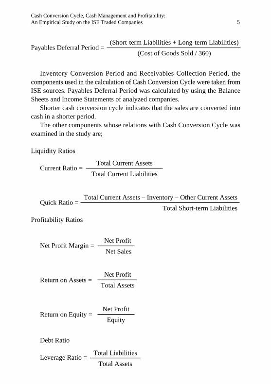
(Short-term Liabilities + Long-term Liabilities)

(Cost of Goods Sold / 360)Payables Deferral Period =

Inventory Conversion Period and Receivables Collection Period, the

components used in the calculation of Cash Conversion Cycle were taken from

ISE sources. Payables Deferral Period was calculated by using the Balance

Sheets and Income Statements of analyzed companies.

Shorter cash conversion cycle indicates that the sales are converted into

cash in a shorter period.

The other components whose relations with Cash Conversion Cycle was

examined in the study are;

Liquidity Ratios

Current Ratio =

Quick Ratio =

Profitability Ratios

Net Profit Margin =

Return on Assets =

Return on Equity =

Debt Ratio

Leverage Ratio =

Total Current Assets

Total Current Liabilities

Total Current Assets – Inventory – Other Current Assets

Total Short-term Liabilities

Net Profit

Net Sales

Net Profit

Equity

Total Liabilities

Total Assets

Net Profit

Total Assets

Cash Conversion Cycle, Cash Management and Profitability: An Empirical Study on the ISE Traded Companies

6

In the study, regression analysis, correlation analysis and comparative

analysis are applied on the basis of two sub-periods, industry and firm size,

by using the variables explained above. The t-test of the sample means was

used in comparative analysis, the relationships were investigated with Pearson

Correlation Analysis and the effect of cash conversion cycle, liquidity and debt

structure on the profitability of the company was measured by regression

analysis. A model was formed for the regression analysis.

Model:

NPM= α + β1 CCC + β2 CR + β3 QR + β4 LR (1)

ROA= α + β1 CC + β2 CR + β3 QR + β4 LR (2)

ROE= α + β1 CCC + β2 CR + β3 QR + β4 LR (3)

Profitability ratios are dependent variables in all models. These profitability

ratios are NPM = Net profit margin, ROA = Return on assets and ROE =

Return on equity. Independent variables in all models are CCC = Cash conversion

cycle, CR = Current ratio, QR = Quick ratio and LR = Leverage ratio.

The data of this study was analyzed by using the SPSS Program.

2.2. Sample and Data Collection Method

The study sample consists of companies whose stocks are listed on the ISE,

excluding holding companies and companies in the finance sector. The 167

sample companies’ balance sheets and income statements for the period of

1995-2000 were used and the data was gathered from ISE's sources. Following

this, a database was formed.

III. Findings

3.1. Descriptive Statistics

In the study, there are statistics that describe the companies on the basis of

investigated variables. As it is presented in Table 1, the mean value of cash

conversion cycle is 78,83 days. Current ratio is 1,71 and quick ratio is 1,08.

The profitability of sample companies was measured by three different ratios.

The mean value of net profit margin is 4,71, but the standard deviation was

found high because the companies are not homogenous, more than one period

was examined and the economic conditions faced by the firms in the study

period. The mean value of return on equity of the sample is 14,11 and the mean

value of return on assets is 7,56. The mean value of the leverage ratio was

found as 55,45 %.


3.2. The Results of Analysis

3.2.1. Comparative Analysis

The research method consists of several comparisons. Firstly, it was investigated

whether the cash conversion cycle, liquidity, profitability and leverage ratios

of the companies differed on the basis of economic period, industry and the

firm size. Due to economic conditions the differences between the periods

were examined. The research period was divided into two sub-periods. The

companies in Turkey operated with high profit margins and showed good

performance during 1995, 1996 and 1997 years. Then they faced economic

recession during the following three-year period (Yücel, 2001). To determine

whether there is any difference between two sub-periods, an analysis was

conducted. The liquidity, profitability and debt structure were investigated for

these two sub-periods. It was found that the mean value of cash conversion

cycle did not indicate a significant difference between two sub-periods. But

current ratio (1,81, 1,61, p= .000), liquidity ratio (1,13; 1,03, p=.012), net profit

margin (10,16; -0,73, p=.000), return on assets (12,45; 2,67, p=.000) and return

on equity (24,57; 3,62; p=.000) decreased and the leverage ratio (52,75; 58,05;

p=.000) increased. In summary, the cash conversion cycle did not vary; liquidity

and profitability ratios decreased and debt ratios of the companies increased

in the recession period.

On the basis of industry, sample companies were categorized into two main

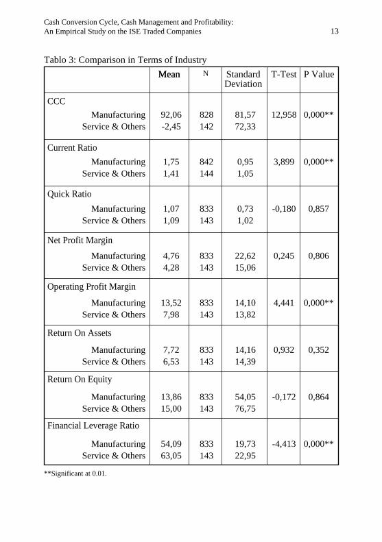
industries: manufacturing and service-other sectors. The findings of our study

suggested that (Annex Table 3) the cash conversion cycle of the manufacturing

industry is longer than the service-other industries (92,06; -2,45, p=.000).

Negative cash conversion cycle is not generally common in the manufacturing

companies. A negative cash conversion cycle can be realized when these

companies have longer payable deferral period than the sum of inventory

conversion period and receivables collection period. Mostly the service sector

companies have negative cash conversion cycles because these companies

have higher inventory turnover and they can collect cash for their services

(Gitman 2000). The result for the sample companies of this study is consistent

with the theory. While manufacturing companies have positive cash conversion

cycle, service companies have negative cash conversion cycle. Current ratio

is higher in the manufacturing sector (1,75; 1,41, p=.000). There is an indication

that liquidity of the manufacturing companies is higher on the basis of current

ratio. There is no statistically significant difference between the industries on

the basis of liquidity ratios, net profit margin, return on assets and return on

equity. In addition, the mean value of leverage ratio of the service industry is


8

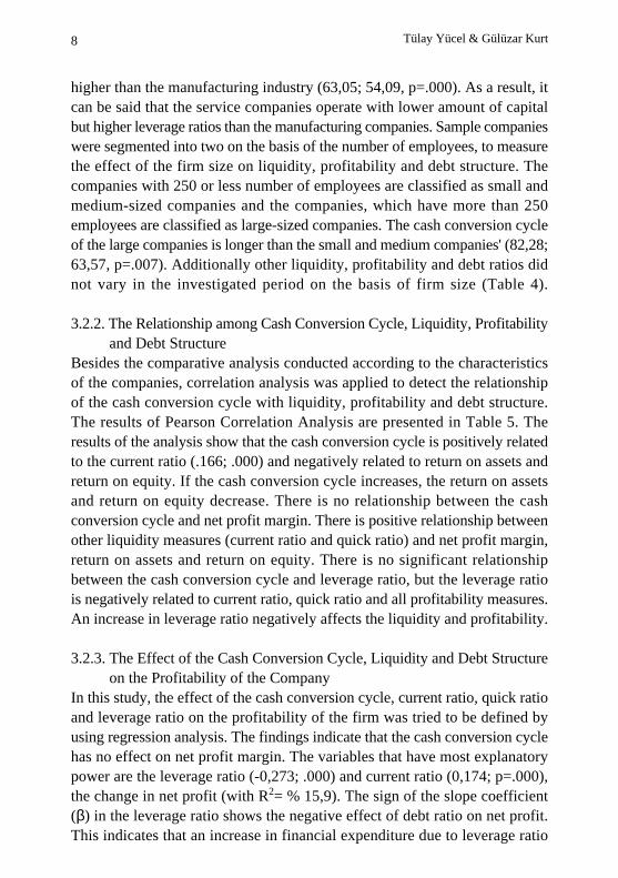
higher than the manufacturing industry (63,05; 54,09, p=.000). As a result, it

can be said that the service companies operate with lower amount of capital

but higher leverage ratios than the manufacturing companies. Sample companies

were segmented into two on the basis of the number of employees, to measure

the effect of the firm size on liquidity, profitability and debt structure. The

companies with 250 or less number of employees are classified as small and

medium-sized companies and the companies, which have more than 250

employees are classified as large-sized companies. The cash conversion cycle

of the large companies is longer than the small and medium companies' (82,28;

63,57, p=.007). Additionally other liquidity, profitability and debt ratios did

not vary in the investigated period on the basis of firm size (Table 4).

3.2.2. The Relationship among Cash Conversion Cycle, Liquidity, Profitability

and Debt Structure

Besides the comparative analysis conducted according to the characteristics

of the companies, correlation analysis was applied to detect the relationship

of the cash conversion cycle with liquidity, profitability and debt structure.

The results of Pearson Correlation Analysis are presented in Table 5. The

results of the analysis show that the cash conversion cycle is positively related

to the current ratio (.166; .000) and negatively related to return on assets and

return on equity. If the cash conversion cycle increases, the return on assets

and return on equity decrease. There is no relationship between the cash

conversion cycle and net profit margin. There is positive relationship between

other liquidity measures (current ratio and quick ratio) and net profit margin,

return on assets and return on equity. There is no significant relationship

between the cash conversion cycle and leverage ratio, but the leverage ratio

is negatively related to current ratio, quick ratio and all profitability measures.

An increase in leverage ratio negatively affects the liquidity and profitability.

3.2.3. The Effect of the Cash Conversion Cycle, Liquidity and Debt Structure

on the Profitability of the Company

In this study, the effect of the cash conversion cycle, current ratio, quick ratio

and leverage ratio on the profitability of the firm was tried to be defined by

using regression analysis. The findings indicate that the cash conversion cycle

has no effect on net profit margin. The variables that have most explanatory

power are the leverage ratio (-0,273; .000) and current ratio (0,174; p=.000),

the change in net profit (with R2= % 15,9). The sign of the slope coefficient

(β) in the leverage ratio shows the negative effect of debt ratio on net profit.

This indicates that an increase in financial expenditure due to leverage ratio


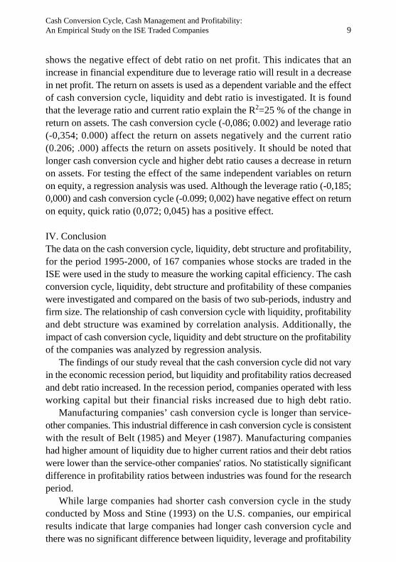
shows the negative effect of debt ratio on net profit. This indicates that an

increase in financial expenditure due to leverage ratio will result in a decrease

in net profit. The return on assets is used as a dependent variable and the effect

of cash conversion cycle, liquidity and debt ratio is investigated. It is found

that the leverage ratio and current ratio explain the R2=25 % of the change in

return on assets. The cash conversion cycle (-0,086; 0.002) and leverage ratio

(-0,354; 0.000) affect the return on assets negatively and the current ratio

(0.206; .000) affects the return on assets positively. It should be noted that

longer cash conversion cycle and higher debt ratio causes a decrease in return

on assets. For testing the effect of the same independent variables on return

on equity, a regression analysis was used. Although the leverage ratio (-0,185;

0,000) and cash conversion cycle (-0.099; 0,002) have negative effect on return

on equity, quick ratio (0,072; 0,045) has a positive effect.

IV. Conclusion

The data on the cash conversion cycle, liquidity, debt structure and profitability,

for the period 1995-2000, of 167 companies whose stocks are traded in the

ISE were used in the study to measure the working capital efficiency. The cash

conversion cycle, liquidity, debt structure and profitability of these companies

were investigated and compared on the basis of two sub-periods, industry and

firm size. The relationship of cash conversion cycle with liquidity, profitability

and debt structure was examined by correlation analysis. Additionally, the

impact of cash conversion cycle, liquidity and debt structure on the profitability

of the companies was analyzed by regression analysis.

The findings of our study reveal that the cash conversion cycle did not vary

in the economic recession period, but liquidity and profitability ratios decreased

and debt ratio increased. In the recession period, companies operated with less

working capital but their financial risks increased due to high debt ratio.

Manufacturing companies’ cash conversion cycle is longer than service-

other companies. This industrial difference in cash conversion cycle is consistent

with the result of Belt (1985) and Meyer (1987). Manufacturing companies

had higher amount of liquidity due to higher current ratios and their debt ratios

were lower than the service-other companies' ratios. No statistically significant

difference in profitability ratios between industries was found for the research

period.

While large companies had shorter cash conversion cycle in the study

conducted by Moss and Stine (1993) on the U.S. companies, our empirical

results indicate that large companies had longer cash conversion cycle and

there was no significant difference between liquidity, leverage and profitability


10

ratios.

The relationship of the cash conversion cycle with liquidity, profitability

and leverage ratios was examined by Pearson correlation analysis. A positive

relationship was found between the cash conversion cycle and current ratio;

it is consistent with Lyroudi and Lazaridu’s study's findings (2000). There was

a negative relationship between cash conversion cycle and return on assets and

return on equity. Longer cash conversion cycle may cause a decrease in return

on assets and return on equity. Though there was no relationship between net

profit margin and cash conversion cycle, there is a positive relationship between

the current and quick ratios are positively related to net profit margin, return

on assets and return on equity. Also, there is no significant relationship between

the cash conversion cycle and the leverage ratios, but the leverage ratio affects

the liquidity ratios and the profitability ratios in a negative way.

Finally, the effect of the cash conversion cycle, liquidity ratios and debt

structure on the profitability was examined. It was found that net profit margin

had a positive association with current ratio and negative association with the

leverage ratio and the cash conversion cycle had no effect on the net profit

margin. The leverage ratio was negatively related to return on assets and return

on equity, but the cash conversion cycle was negatively related to return on

assets and return on equity. Longer cash conversion cycle had a negative effect

on the profitability.

ReferencesBelt, Brian, “The Trend of the Cash Conversion Cycle and its Components”, Akron Business

and Economic Review, Fall 1985, pp 48-54.

Besley, Scott, E. F. Brigham, Essentials of Managerial Finance, The Dryden Press, USA,

2000.

Besley, Scott, R. L. Meyer, “An Empirical Investigation of Factors Affecting the Cash

Conversion Cycle”, presented at the Annual Meeting of the Financial Management

Association, Las Vegas, Nevada, October 1987.

Gentry, James A., R. Vaidyanathan, Hei Wee Lee, “A weighted Cash Conversion Cycle”,

Financial Management, Spring 1990, pp 90-99.

Gitman, L. J., Principles of Managerial Finance, Addison Wesley Longman, USA, 2000.

Kamath, R., “How Useful are Common Liquidity Measures?”, Journal of Cash Management,

January/February 1989, pp 24-28.

Lyroudi, K., J. Lazaridis, "The Cash Conversion Cycle and Liquidity Analysis of the Food

Industry in Greece", http://papers.ssm.com/paper.tafabstract_id=236175, 14 Ocak

2002.

Lyroudi, K., D. McCarty, “An Empirical Investigation of the Cash Conversion Cycle of

Small Business Firms”, The Journal of Small Business Finance, Vol. 2, 2, 1992/1993,


pp 139-161.

Moss, D. J., B. Stine, “Cash Coversion Cycle and Firm Size: A Study of Retail Firms”,

Managerial Finance, Vol. 19, Issue 8, 1993, pp 25-31.

Richards, V. D., Laughlin, E. J., “A Cash Conversion Cycle Approach to Liquidity Analysis”,

Financial Management, Spring 1980, pp 32-38.

Shin, Hyun-Han, L.Soenen, "Efficiency of Working Capital Management and Corporate

Profitability", Financial Practice & Education, Fall/Winter 98, Vol. 8, Issue 2, pp

37, 9p.

Shin, Hyun-Han, L.Soenen, "Liquidity Management or Profitability - Is There Room for

Both?", AFP Exchange, Spring 2000, Vol. 20, Issue 2, pp 46, 4p.

Smith, Keith, “Profitability Versus Liquidity Tradeoffs in Working Capital Management”,

in K. V. Smith, Readings on the Management of Working Capital, St. Paul, MN,

West Publishing Company, 1980, 549-562.

Yücel, T., Firms' Response to Economic Crises, An Emprical Study on ISO Market,

ERC/METU, International Conference in Economics V, Ankara, September 10-13,

2001.


12

ANNEX

Table 1: Sample/Selected Firms’ Characteristics (1995-2000)

*Significant at 0.05.**Significant at 0.01.

Variables Mean MedianStandard Deviation N

Cash Conversion Cycle 78,83

1,71

1,08

4,71

12,78

7,56

14,11

55,45

74,76

1,50

0,92

5,89

13,53

7,18

17,84

55,52

87,04

0,98

0,78

21,61

14,18

14,16

57,73

20,43

976

982

982

982

982

992

982

993

Quick Ratio

Net Profit Margin

Operating Profit Margin

Return On Assets

Return On Equity

Financial Leverage Ratio

Current Ratio

CCC

Current Ratio

Quick Ratio

Net Profit Margin


Return On Assets

Return On Equity


Tablo 2: Comparison Between the Periods

1995-1997

1998-2000

1995-1997

1998-2000

1995-1997

1998-2000

1995-1997

1998-2000

1995-1997

1998-2000

1995-1997

1998-2000

1995-1997

1998-2000

1995-1997

1998-2000

Mean Standard Deviation

N T-Test P Value

80,0577,96

1,811,61

1,131,03

10,16-0,73

16,648,93

12,452,67

24,573,62

52,7558,05

484

493

490

490

490

490

490

490

84,5289,31

1,010,94

0,800,77

10,4427,72

14,0613,26

10,4015,68

34,1872,78

19,6320,85

0,526

3,72

2,507

8,800

10,79

13,919

6,023

-7,019

0,599

0,000**

0,012*

0,000**

0,000**

0,000**

0,000**

0,000**


13

Tablo 3: Comparison in Terms of Industry

**Significant at 0.01.


N T-Test P Value

92,06

-2,45

1,75

1,41

1,07

1,09

4,76

4,28

13,52

7,98

7,72

6,53

13,86

15,00

54,09

63,05

828

142

842

144

833

143

833

143

833

143

833

143

833

143

833

143

81,57

72,33

0,95

1,05

0,73

1,02

22,62

15,06

14,10

13,82

14,16

14,39

54,05

76,75

19,73

22,95

12,958

3,899

-0,180

0,245

4,441

0,932

-0,172

-4,413

0,000**

0,000**

0,857

0,806

0,000**

0,352

0,864

0,000**

CCC

Current Ratio

Quick Ratio

Net Profit Margin


Return On Assets

Return On Equity


Manufacturing

Service & Others

Manufacturing

Service & Others

Manufacturing

Service & Others

Manufacturing

Service & Others

Manufacturing

Service & Others

Manufacturing

Service & Others

Manufacturing

Service & Others

Manufacturing

Service & Others

Mean


0,0240,463

0,570** 0,000

0,5000,000

-0,370**0,000

-0,176**0,000

-0,470**0,000

-0,222**0,000

1,000

14

Tablo 4: Comparison in Terms of Firm-size

Table 5: Correlation Analysis

Cash ConversionCycle

Current Ratio

Quick Ratio

Net Profit Margin


Return On Assets

Return On Equity


0,166**0,000

1,000

0,913**0,000

0,331**0,000

-0,0320,317

0,396**0,000

0,153**0,000

0,570**0,000

Cash Conversion Cycle

Current Ratio

Quick Ratio

Return On Equity

Net Profit Margin


Return OnAssets

1,000

0,166**0,000

0,0400,210

0,0310,329

0,0170,585

-0,0590,064

-0,100**0,002

0,0240,463

0,0400,210

0,913**0,000

1,000

0,310**0,000

-0,0570,074

0,375**0,000

0,162**0,000

0,500**0,000

0,0310,329

0,331**0,000

0,310**0,000

1,000

0,523**0.000

0,817**0,000

0,1320,000

-0,370**0,000

-0,0590,064

0,396**0,000

0,375**0,000

0,8170,000

0,577**0,000

1,000

0,326**0,000

-0,470**0,000

-0,100**0,002

0,153**0,000

0,162**0,000

0,132**0,000

0,322**0,000

0,326**0,000

1,000

-0,222**0,000

**Significant at 0.01.

CCC

Current Ratio

Quick Ratio

Net Profit Margin


Return On Assets

Return On Equity



N T-Test P Value

63,5782,28

1,641,68

1,010,78

4,404,73

12,0313,54

6,297,96

9,5914,67

55,8655,35

213733

219743

214738

214738

214738

214738

214738

219744

91,2779,98

0,950,82

1,050,65

20,6621,94

15,7811,59

15,3813,85

82,5348,33

22,2819,51

-2,704

-0,535

-0,837

-0,203

-1,298

-1,431

-0,859

0,305

0,007*

0,593

0,403

0,839

0,195

0,153

0,391

0,761

Small & Medium-SizedLarge-Sized









0,0170,585

0,0320,317

-0,0570,074

0,523**0,000

1,000

0,577**0,000

0,322**0,000

-0,176**0,000


15

Regression Results

NPM = α + β1LR + β2CR

Dependent Variable: Net Profit Margin

LR

CR

Constant: 14,282

F: 91,843

P: 0,000

Adj. R2: 0,159

T Pβ

-0,273

0,174

-7,606

4,841

0,000

0,000

ROA = α + β1LR + β2CCC + β3 CR

Dependent Variable: Return On Assets

LR

CCC

CR

Constant: 17,278

F: 110,289

P: 0,000

Adj. R2: 0,252

T Pβ

-0,354

-0,086

0,206

-10,355

-3,033

5,948

0,000

0,002

0,000

ROE = α + β1LR + β2QR

Dependent Variable: Return On Equity

LR

CCC

QR

Constant: 42,772

F: 21,728

P: 0,000

Adj. R2: 0,060

T Pβ

-0,185

-0,099

0,072

-5,145

-3,183

2,007

0,000

0,002

0,045


Assc. Prof. Dr. Y›ld›r›m B. Önal, Çukurova University, Faculty of Economics and Administrative Sciences, Department of Business, 01330, Adana/Turkey.Tel: 0322 338 72 54 Fax: 0322 338 72 83 E-mail: [email protected]. Prof. Dr. Murat Do¤anlar, Çukurova University, Faculty of Economics and Administrative Sciences, Dept. of Economics, 01330, Adana/Turkey. Tel: 0322 338 72 54 Fax: 0322 338 72 84 E-mail: [email protected] Prof. Dr. Serpil Canbafl, Çukurova University, Faculty of Economics and Administrative Sciences, Dept. of Business, 01330, Adana/Turkey. Tel: 0322 338 72 54 Fax: 0322 338 72 84 E-mail: [email protected]

*

**

***

MEASUREMENT OF FOREIGN EXCHANGE

EXPOSURE ON THE

TURKISH PRIVATE BANKS’ STOCK PRICES

Abstract All performance criteria of the banks are affected by the exchange rate fluctuations

through foreign currency transactions and operations. However, exchange rate

fluctuations -even without such activities can influence the banks through their

affect on foreign competition, foreign loan demand and other banking conditions.

Exchange rate exposure is classified as operation, transaction, and accounting

exposures. Most of the studies, which measure these exposures, focused on the

affect of the exchange rate exposure on the value and stock price of the firm.

High inflation rates, a highly volatile foreign exchange market, increasing

tendency of the banking system to work with exchange rate exposure and the

absence of sufficient instruments to cover the exchange rate risk can explain

the importance of the foreign exchange exposure in Turkey. Turkish banking

system that is the biggest actor in the financial system operates with exchange

rate exposure and therefore it is important to analyze the effect of the exchange

rate risk on the Turkish banking system. For this purpose, a cointegration model

has been estimated to analyze the effect of unanticipated changes in the exchange

rate on the stock prices of the 11 commercial banks, which were quoted in the

Istanbul Stock Exchange Market.

Y›ld›r›m B. ÖNAL* Murat DO⁄ANLAR**Serpil CANBAfi***


ISSN 1301-1642 © ISE 1997

I. Introduction

After the collapse of the Bretton Woods, most countries adopted the flexible

exchange rate systems and abandoned the adjustable peg, which caused many

firms (mostly multinational) to face the problem of foreign exchange exposure.

Foreign exchange risk, in general, effects the cash flows and therefore the

value of the firms. In other words, foreign exchange risk that occurs as a result

of unanticipated changes in the exchange rate affects all firms and the sectors

in the economy. However, mostly multinational companies, and banks that

deal with foreign currency transactions and foreign operations are affected by

the uncertainty in the exchange rates. Exchange rate exposure is classified as

operation, transaction, and accounting affects. Most of the studies, which

measure these affects, focused on the impact of the exchange rate exposure on

the firm value and the stock price of the company.

All performance criteria of the banks are affected by the exchange rate

fluctuations through foreign currency transactions and operations. However,

exchange rate fluctuations -even without such activities can influence the banks

through their affect on foreign competition, foreign loan demand and other

banking conditions.

High inflation rates, highly volatile foreign exchange market, increased

tendency of the banking system to work with exchange rate exposure and

absence of sufficient instruments to cover the exchange rate risk can explain

the importance of the foreign exchange exposure phenomenon in Turkey.

Turkish banking system that is the biggest actor in the financial system operates

with exchange rate exposure and therefore it is important to analyze the effect

of the exchange rate risk on the Turkish banking system. For this purpose, a

cointegration model has been estimated to analyze the effect of foreign exchange

risk on the stock prices of the 11 private deposit banks, which were quoted on

the Istanbul Stock Exchange Stock Market (ISE).

The first step in the empirical section of the study is to analyze if the

variables contain a unit root. The next is to estimate a cointegration model to

examine the effect of unanticipated changes on the stock prices of these banks

in the long-run.

The next section is devoted to explain the concept of foreign exchange

exposure. Section three reviews the empirical literature. Section four analyses

the effect of unanticipated changes in the exchange rate on these banks and

the final section presents the conclusion.

II. Foreign Exchange Exposure

Foreign exchange exposure occurs as a consequence of the unanticipated

18 Y›ld›r›m B. Önal & Murat Do¤anlar & Serpil Canbafl

changes in the exchange rate. Anticipated changes in the exchange rate do not

contain any risk for individuals, companies, or governments.

In general, foreign exchange exposure is described as the statistical variance

of the domestic-currency value of an asset, liability or operating income, which

is attributable to unanticipated changes in exchange rates (Levi, 1996; Adler

and Dumas, 1984). Foreign exchange exposure affects all sectors and firms

in the economy. In addition to this it is more effective on the firms, which

operate internationally and/or which demand foreign loans. Foreign exchange

exposure can result from different sources. i) The most common type of foreign

exchange exposure results from trade flows. This happens when the firms

realize at least some of their sales and/or costs such as raw materials in terms

of a foreign currency. ii) Another source of the exposure is owning a foreign

subsidiary. This type of exposure occurs in two different ways. The first one

is called as the profit translation, which is the value in the currency of the

parent company of a constant stream of profits from the foreign subsidiary

that will change along with a change in the foreign exchange rate. The second

way of exposure is called the balance sheet exposure. This occurs when the

balance sheet value of the foreign subsidiary in the parent company’s currency

will change due to changes in exchange rates. iii) Exposure may appear as a

result of borrowings in foreign currency. Because, firms may not always find

foreign funds in their national currencies. iv) Finally, the least type of the

exposure is the strategic exposure. This occurs as a result of the large currency

movements. The Asian crisis is an example for this type of exposure. Large

currency devaluations were experienced in the Asian crises, which harmed

many firms. The firms in these countries reduced their scales, or were closed

or the owner of the firms changed after the crises (Asiamoney, 1997/1998).

Foreign exchange risk and foreign exchange exposure are related concepts

but they should be evaluated differently. Mostly, these two concepts are used

interchangeably. However, foreign exchange exposure is defined as the

sensitivity of changes in the real domestic-currency value of assets, liabilities

or operating incomes to unanticipated changes in the exchange rate (Altay,

1999; Levi, 1996).

Foreign exchange exposure for the firms can be measured in three different

ways. These are transaction exposure, operating exposure (these two types of

exposure comprise the economic exposure), and translation/accounting exposure

(Eiteman et al, 1998). Operating exposure measures the change in value of the

firm, which occurs as a result of changes in the future operating cash flows

caused by an unexpected change in exchange rates. Transaction exposure

measures changes in the value of outstanding financial obligations contracted

19Measurement of Foreign Exchange Exposure on the Turkish Private Banks’ Stock Prices

20

before a change in exchange rates but not due to be settled until after the

exchange rate change. Transaction exposure concerns changes in the cash

flows that result from existing business liabilities. Translation/accounting

exposure occurs as a result of the need to translate foreign currency financial

statements into a single reporting currency.

The foreign exchange exposure, which is caused by the unexpected changes

in foreign exchange rates force the companies to manage the foreign exchange

exposure. But for an effective strategy, the management should determine

what is under risk. This task can be accomplished by a group of staff that tries

to maintain the cash flow according to economic and financial realities, while

the other group of staff should try to protect their companies from the

translation/accounting exposure.

Since accounting techniques –no matter how perfect these techniques are-

depend on historical records, they cannot measure properly the effect of the

unanticipated changes in the exchange rate on the future cash flows of the

firms. Therefore, the companies should be protected from the effect of

unanticipated changes of the exchange rates on their market values and also

the cash flows should be protected from the economic exposure, which occurs

as a result of operating and transaction exposures. This is accepted as the most

appropriate strategy, which aims at maximizing the net present value of the

future cash flows.

Balanced foreign exchange positions of the banks show that they are not

under risk. On other hand, they can face foreign exchange exposure, which

depends on their short or long position caused by foreign exchange operations.

The risks of the banks that they can face according to foreign exchange

operations can be grouped in three different ways. The first of these is the

credit risk. The credit risk can occur when the credits are in foreign currency.

These types of operations cause foreign exposure for the banks in the repayment

of their debts. Second type is the exchange rate risk. In order to meet the

demands of their customers, banks can buy or sell foreign currency. If the

banks cannot balance their foreign currency accounts, they can be affected

from the fluctuations in the exchange rates. The last type of the risk is liquidity

risk. Banks can use their accounts at the Central Bank or at domestic or foreign

correspondents in order to realize their credit, deposit, debt and interest payments

in foreign currency, on time. The imbalances occurring due to these types of

foreign currency transactions can cause foreign exchange exposure for the

banks (Altay, 1999). Existence of the foreign exchange exposure may influence

the stock prices as well as the values of the firms. Therefore, firm managers

should take into consideration the effects of these types of risks on the stock


prices and values of their firms.

III. Review of the Empirical Literature

There are several studies in the literature, which identify the foreign exchange

exposure and explain its affect from different perspectives. This section presents

a summary of the selected studies.

Adler and Dumas (1984) explain the differences between foreign exchange

rate risk and foreign exchange exposure. Here, foreign exchange risk is defined

as the unexpected changes in the exchange rate and the foreign exchange

exposure indicates the coefficient of the simple regression between exchange

rate changes and prices or returns. They measured the foreign exchange exposure

on the foreign currency basis. They emphasized that this is the amount, which

should be protected from foreign exchange rate changes. They measured the

foreign exchange exposure by dividing the covariance between exchange rates

and stock prices by the variance of the exchange rate cov(P,S)/var(S).

Jorion (1990) measured the flexibility of the multinational US companies

to the foreign exchange exposure. It was claimed that the value of a firm is

related to the flexibility of the fluctuations in the foreign exchange rates and

the foreign exchange exposure is measured as the regression coefficient, which

determines the change in the value of the firm. The model was constructed as

follows: Rit = β0i + β1i Rst + εit where Ri shows the rate of return of the firm

and Rs shows the trade weighted exchange rate. It is known that multinational

companies protect themselves from operational and accounting effects by using

various instruments. If the activities of protection from the risk are known and

added to the stock prices, then this would weaken the correlation between the

stock prices and the foreign exchange rate. Another important issue is that the

ratio of foreign revenue to the total revenue, which is important for the foreign

exchange exposure, was replaced with the ratio of foreign sales to the total

sales. It was shown that foreign exchange exposure is also related to this ratio.

Jorion also found that there were cross section foreign exchange exposure

differences in the multinational US companies. However, it was found that

foreign exchange exposure of the US multinationals was related to the share

of their foreign sales in the total sales. It was also found that companies, which

do not have foreign transactions, were also affected by the foreign exchange

exposure.

Jorion (1991) analyzed the pricing of foreign exchange exposure in US

stock market by using two factors and multi-factor pricing models in his study.

The results showed that the relation between the value of the US dollar and

returns of stocks is systematically changing on industrial basis. In addition to


22

this, the empirical results of this study showed that the foreign exchange

exposure was not priced in the stock market. In other words, unconditional

risk premium related to the foreign exchange exposure was found to be small

and statistically insignificant. 20 different industrial portfolios from the New

York Stock Exchange were constituted. Both the two factor and the six factor

models were applied to these 20 industry portfolios. The important findings

are: i) a positive foreign exchange exposure was found in the chemical and

machinery industries (these are exporting industries) for both models. ii) a

negative foreign exchange exposure was found in the textile and the hypermarket

industries (these are importing industries) and iii) Foreign exchange exposure

for the rest of the industries was found to be insignificant. There is no systematic

relationship between foreign exchange exposure and stock returns in general.

The results suggest that US investors do not price foreign exchange exposure.

Bartov and Bodnar (1994) investigated the relationship between foreign

exchange rate changes and abnormal returns in the multinational companies.

It is widely known that the changes in the foreign exchange rates affect the

values of the firms. However, the past empirical studies could not find any

relation that the foreign exchange rate changes result in a change in the current

value of the firms. They claim that there are two possible causes for that. First

of these is selecting a wrong sample, that is, the selected firms had either weak

international relations or the foreign exchange exposure is in a different

direction. The second cause is systematic mispricing which means that a change

in the current value of the firm might result from the lagged changes in the

foreign exchange rate. Although, this study could not find any relationship

between abnormal returns of the firms and current exchange rate changes, it

was found that abnormal return and lagged exchange rate changes were related.

It is possible to conclude that investors cannot use all available information

on time. Current data for investment decision is used with a delay, however

past information determines the present investment decisions.

Chamberlain et al (1997) examined the foreign exchange exposure for a

sample of US and Japanese banking institutions. Daily data was used to estimate

the exchange rate sensitivity of the equity returns of the US banks and to

compare them with those of the Japanese banks. It was found that the stock

returns of a significant fraction of the US companies move in line with the

exchange rate, while a few of the Japanese returns were observed to do so.

This study i) was able to discern exchange rate exposure among individual US

banks. This study also used daily observations instead of monthly observations,

which increased the power of the tests. ii) A link between foreign exchange

exposure and stock returns was found. The results also provided some insights


into the usefulness of accounting indicators. iii) estimated the exchange rate

exposure for Japanese banks and compared it with US banks. It was also found

that using daily data, the stock returns of approximately one third of the large

US bank holding companies were sensitive to exchange rate changes. In

contrast, a few Japanese bank returns were found to be sensitive to exchange

rate changes.

Merikas (1999) investigated the structural relationship between the exchange

rate exposure and the stock value of the Greek banking institutions. Although,

exchange rate is a significant determinant of the bank returns, an augmented

market model was used since exchange rate is not the only parameter to

determine the returns. The estimated equation included the general index of

the Athens Stock Exchange as one of the independent variables to represent

the market return (Rm). In order to provide control over the sources of the

sectoral variations in returns such as changes in the interest rates, sectoral bank

index (Rb) was also incorporated into the analysis as a second independent

variable. Third independent variable is nominal exchange rates (S1=USD,

S2=DEM, S3=JPY). The estimated model is as follows (Rt = α0 + α1 Rm +

α2 Rb + α3 S1 + α4 S2 + α5 S3 + Ut), and the variables used in the analysis

were checked for stationarity. The long-run relationship was checked among

the variables. The analysis was conducted on a daily basis and covers the

period between August 1995- November 1998. The empirical results indicated

that the stock returns of the Greek banks were directly influenced by the three

major currencies.

Altay (1999) analyzed the effects of the real exchange rate exposure on the

real returns of the stocks in the ISE. The relationship between real stock returns

of 50 different companies and the changes in the real exchange rate were

analyzed by using 10 different models. The period under analysis is 1991-

1996. The results are as follows: i) the explanatory power of the exchange rate

changes on the stock returns was between 0.58 % and 14.58 %. This result

indicated that the exchange rate changes could not explain the stock returns.

ii) changes in the exchange rate effects only 4 firms out of 50, which indicated

that stock returns or pricing of the stock returns were not affected by the

exchange rate exposure. iii) the foreign exchange exposure was found to be

unrelated to the degree of openness. iv) protection from the foreign exchange

exposure in the ISE depends on other factors and therefore this effect was

taken into consideration in pricing. It was also concluded that absence of a

forward market limited the analysis to measure the effect of the foreign exchange

exposure on the stock returns.

Gao (2000) studied the manufacturing multinational companies. Unlike the


24

other studies, this study considered the time variability of exchange rate

exposure by including foreign sales and foreign production information in the

analysis. The ratios used in the analysis were i) export/total output, ii)

import/import + total output, iii) foreign sales/total sales, iv) foreign assets/total

assets and, v) number of companies in the sample. The effect of the exchange

rate movements on the profitability of the firms had important implications

for macroeconomic theory and policy, and also for the decisions of the firms

on production, sales, pricing policy, and financial operation. Empirical results

indicate that effect of the exchange rate changes on the profitability is less than

its effect on the production. This study proposed a model relating exchange

rate exposure to foreign sales and production of a multinational firm. Theory

predicts that unexpected changes in the exchange rate increase the foreign

sales of the firm, but decrease the foreign assets. The overall impact of the

exchange rate is the sum of these two opposite effects. The model was applied

for a sample of 80 multinational firms. The results suggested that profitability

of the firms were effected by the unexpected changes in the exchange rates as

predicted by theory and the results were found to be statistically significant.

Martin (2000) studied the exchange rate exposure for each important

financial institution by assessing country-specific portfolios and global portfolios.

It was found that more than 40 percent of the important financial institutions

were exposed to changes in the value of their domestic currencies. Almost 60

percent of the key institutions and 75 percent of the key non-US institutions

were affected by the changes in the value of the US dollar. The results also

revealed that US portfolios are less exposed than the other countries’ portfolios

and it was claimed that this might be attributed to more restrictive regulatory

and supervisory requirement implied on US institutions.

Allayannis and Ihrig (2000) examined proper specification and testing for

the factors that affect the exchange rate exposure of the stock returns. They

developed a theoretical model, which defined three channels of exposure. It

was claimed that exposure in an industry increases where the final output is

sold i) by greater competitiveness in the market, ii) the interaction of greater

competitiveness in its exports and a higher share of exports in production, iii)

the interaction of lower competitiveness in the imported input market and the

smaller the share of imports in production. The sample covered 82 US

manufacturing industries classified at the 4-digit SIC level and 18 industry

groups in 2-digit SIC level between 1979 and 1995. It was found that exchange

rate movements for a firm are an important source of risk. Stock returns

instantaneously adjust to an unanticipated change in the exchange rate in

efficient markets. However, it takes a considerable time for investments to


adjust. It was found that 4 industry groups out of 18 were significantly exposed

to exchange rate changes through one of the channels of exposure. The results

indicated that a one-percent appreciation of the dollar decreases the return of

the average industry by 0.13 percent.

IV. Testing the Foreign Exchange Exposure on the Turkish Commercial Banks’

Stock Prices

Although the Turkish banking system works under tight regulations, the banking

institutions operate with foreign exchange exposure, which constitutes about

30 percent of their equities. Therefore, as the international financial institutions

have also mentioned, the Turkish banks are exposed to the foreign exchange

risk (IMF, International Capital Markets, 1999).

This section of the study will analyze the foreign exchange exposure of the

Turkish commercial banks, which have a significant weight in Turkish financial

system.

4.1. Scope of the Study and Data

The purpose of this study is to analyze the effect of the unanticipated changes

in the exchange rate on the stock prices of the Turkish Banks. Therefore, 11

commercial banks have been included in the analysis that has been quoted in

the (ISE) for the period under analysis. The analysis has been conducted on

a monthly basis, which covers the period between May 1994- May 2000. The

reason for choosing this period is to exclude the effects of 1994 and 2001

crises from the estimation period. Initially, both the US Dollar and the German

Mark were included into the analysis. However, high degree of correlation

between the German Mark and the US dollar (over 80 percent correlation)

indicated to include only one of these variables. Therefore, the US Dollar was

used to represent the impact of exchange rate changes. A similar correlation

was found between the ISE Financials Index and the ISE National-100 Index.

Therefore, it was decided to use the National-100 Index instead of using both

indices. The high degree of correlation between the National-100 Index and

the Financials Index can easily be seen below in Graphic 1. The data used in

the estimation are stock market prices of the banks under investigation, the

ISE National-100 Index, and Lira-Dollar nominal exchange rate. The data

were obtained from the web pages of the Istanbul Stock Exchange Market and

Analiz Yat›r›m Araflt›rmalar› A.fi.


Graphic 1: ISE National-100 and ISE Financial Index

4.2. Model

The model used by Merikas (1999) has been used in the empirical analysis in

order to determine the effect of the unanticipated changes in the exchange rate

on the stock prices of the 11 banks under analysis. The stock price of each

bank (R) is determined by the unanticipated changes in the exchange rate (S)

and the ISE National-100 Index (U), which is accepted to represent the general

market index.

Moving sample standard deviation of the nominal exchange rate has been

used as the proxy variable to represent the volatility term. (ner) denotes the

nominal exchange rate and m is determined by using Akaike information

criterion (Karasoy, 1995) and the value of m was determined to be 12 in our

analysis.

Johansen cointegrating technique is used to analyze the long-run relationship

among the stock prices, general index, and exchange rate risk. Time series

methods have been widely discussed in the literature, therefore, the results will

be presented without explaining the details of this method.

Stationarity of the variables used in the analysis was determined by using

Augmented Dickey-Fuller (ADF) tests and it was found that all series have

unit root processes. This indicates that the series are stationary in their first

26

Rt = β0 + β1(St) + β2(Ut) + et

St = [(1/m) ∑ (In nert – In nert-1 )2 ]

1/2m

i=1


11

10

9

8

7

6

51997 1998 19991996

Financal National-100

2000

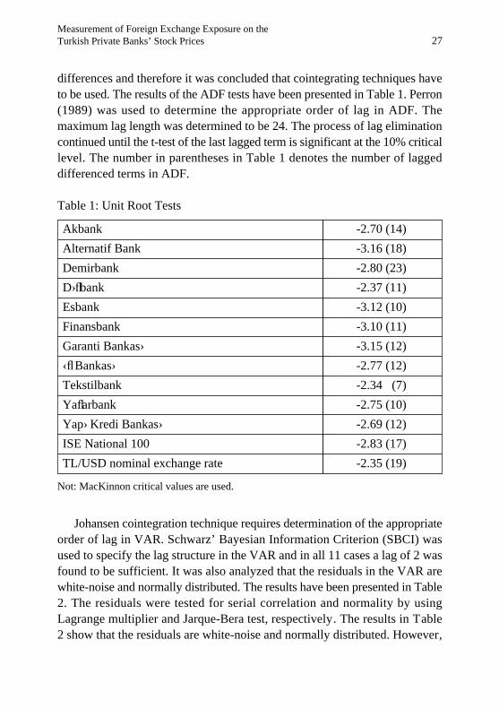
differences and therefore it was concluded that cointegrating techniques have

to be used. The results of the ADF tests have been presented in Table 1. Perron

(1989) was used to determine the appropriate order of lag in ADF. The

maximum lag length was determined to be 24. The process of lag elimination

continued until the t-test of the last lagged term is significant at the 10% critical

level. The number in parentheses in Table 1 denotes the number of lagged

differenced terms in ADF.

Table 1: Unit Root Tests

Johansen cointegration technique requires determination of the appropriate

order of lag in VAR. Schwarz’ Bayesian Information Criterion (SBCI) was

used to specify the lag structure in the VAR and in all 11 cases a lag of 2 was

found to be sufficient. It was also analyzed that the residuals in the VAR are

white-noise and normally distributed. The results have been presented in Table

2. The residuals were tested for serial correlation and normality by using

Lagrange multiplier and Jarque-Bera test, respectively. The results in Table

2 show that the residuals are white-noise and normally distributed. However,

27

Akbank

Alternatif Bank

Demirbank

D›flbank

Esbank

Finansbank

Garanti Bankas›

‹fl Bankas›

Tekstilbank

Yaflarbank

Yap› Kredi Bankas›

ISE National 100

TL/USD nominal exchange rate

-2.70 (14)

-3.16 (18)

-2.80 (23)

-2.37 (11)

-3.12 (10)

-3.10 (11)

-3.15 (12)

-2.77 (12)

-2.34 (7)

-2.75 (10)

-2.69 (12)

-2.83 (17)

-2.35 (19)

Not: MacKinnon critical values are used.

Measurement of Foreign Exchange Exposure on the Turkish Private Banks’ Stock Prices

the normality assumption for the residuals was not satisfied in case of Yaflarbank1

Addition of higher lags in the VAR did not change the results. The results for

other cases are satisfactory and the lag specifications are adequate.

Table 2: Diagnostic Statistics for the Residuals

Results of the Johansen cointegrating technique have been presented in

Table 3. Both maximum eigenvalue and trace test results failed to find a long-

run equilibrium relationship between stock prices of 9 banks and exchange

rate risk. However, a long-run equilibrium relationship between stock prices

of Esbank and Yaflarbank and the exchange rate risk term was found. The

analysis was conducted under the assumption that the data have linear

deterministic trends.

28

Results of the Jarque and Bera test should be interpreted carefully. Because, the test is nonconstructive. If the test result does not show that the series are not normally distributed, it does not indicate the next step . Another point which should be noted is that, even if the test result suggests nonnormality, it does not confirm it (Green, 1993, p.310).

1


Akbank

Demirbank

D›flbank

Finansbank

Garanti Bankas›

‹fl Bankas›

Yaflarbank


Alternatif Bank

Esbank

Tekstilbank

J - B

1.13

3.31

3.71

4.78

1.97

5.48

10.6

2.17

2.05

0.13

1.04

AR (1)

1.08

0.47

0.87

0.02

0.01

0.21

0.38

0.44

1.50

0.01

0.01

AR (2)

2.01

0.53

0.98

0.45

1.66

3.13

0.51

0.65

2.54

0.06

0.02

Table 3: Johansen Cointegration Analysis

Notes: Critical values for trace test and maximal eigenvalue tests at %5 level of significance

are 42.44 and 25.54, respectively.

*indicates significant at 5% level.

The long-run coefficients normalized with respect to the Yaflarbank stock

prices are presented below.

Ryaflarbank = -9.52 –0.92 (S) + 0.24 (U)

The long-run coefficients normalized with respect to the Esbank’s stock

prices are presented below.

Resbank = -3.44 –0.98 (S) - 0.75 (U)

The long-run coefficients of the risk term are 0.92 and 0.98, which indicate

that there is almost a one to one effect of the unanticipated changes in exchange

rate on the stock prices of the two banks in the long-run. The error correction

models can be estimated as follows. The coefficient of the error correction

term (ect-1) is (-0.54) which shows a slow speed of adjustment. The sign of

this term is correct and it is significant. The values in parentheses are t-statistics.


Akbank

Demirbank

D›flbank

Finansbank

Garanti Bankas›

‹fl Bankas›

Yaflarbank


Alternatif Bank

Esbank

Tekstilbank

Trace Test

37.41

35.56

35.07

32.94

32.41

32.12

47.94*

34.41

26.10

46.01

34.18

Max. Eigenvalue

24.67

21.83

22.21

17.75

19.15

17.22

26.79*

24.37

15.15

24.45

18.06

Application of the error correction model for Esbank shows a coefficient

of (-0.72) for the error correction term and this term has also the right sign and

is statistically significant. The speed of adjustment is also slow in the case of

Esbank although it is faster than Yaflarbank.

A long-run equilibrium relationship was not found between exchange rate

risk term and the stock prices for the other 9 banks namely, Akbank, Demirbank,

D›flbank, Finansbank, Garanti Bankas›, ‹fl Bankas›, Yap› Kredi Bankas›,

Alternatifbank and Tekstilbank. These findings indicate that these banks’ stock

prices have not been affected by the unanticipated changes in the exchange

rate in the long-run. In other words, these banks’ stock prices may not be

subject to foreign exchange exposure in the long-run.

III. Conclusion

Turkish economy has experienced a prolonged economic crisis. Financial

markets and especially the banking sector, which is the main actor of the

financial markets, were severely hit by the crises. As it is widely accepted,

any crises in the financial sectors intensify the crises in the real sectors of the

economy. This study aimed at analyzing the foreign exchange exposure of the

Turkish banking sector.

A long-run relationship between unanticipated exchange rates and stock

prices of the banking institutions was examined. Empirical results showed that

a long-run relationship between unanticipated exchange rates and stock prices

was found only for Yaflarbank and Esbank out of 11 cases. It was found that

Akbank, Demirbank, D›flbank, Finansbank, Garanti Bankas›, ‹fl Bankas›, Yap›

Kredi Bankas›, Alternatifbank, and Tekstilbank were not affected by the

unanticipated changes in the exchange rate in the long-run.

The analysis covered the period between two recent currency crises in

30 Y›ld›r›m B. Önal & Murat Do¤anlar & Serpil Canbafl

∆Ryaflarbank = -0.54 (ect-1) + 0.12(∆Rt-1) + 0.43(∆Rt-2) + 0.67(∆Ut-1) – 0.35(∆Ut-2)

(-4.12) (0.65) (2.56) (2.92) (-1.46)

- 4.53(∆St-1) – 1.48(∆St-2)

(-0.59) (-0.20)

∆Resbank = -0.72 (ect-1) + 0.20(∆Rt-1) + 0.34(∆Rt-2) + 0.04(∆Ut-1) – 0.40(∆Ut-2)

(-3.33) (0.90) (1.75) (0.19) (-1.91)

- 1.06(∆St-1) – 5.26(∆St-2)

(-0.16) (-0.82)

Turkey. Therefore, the findings of this study are supported by the current

status of the banking sector. In other words, Yaflarbank and Esbank were

transferred to Saving Deposit Insurance Fund (SDIF) and we found in our

analysis that these two banks are affected by the unanticipated changes in the

exchange rates in the long-run. Currently, the other 9 banks namely Akbank,

D›flbank, Finansbank, Garanti Bankas›, ‹fl Bankas›, Yap› Kredi Bankas›,

Alternatifbank, and Tekstilbank (except Demirbank)2, still operate in the sector

under unfavorable economic and financial conditions and this also supports

our findings.

ReferencesAdler, M., Dumas B., “Exposure to Currency Risk: Definition and Measurement”, Financial

Management, Summer, 13, 1984, p.41-50.

Allayannis, G., Ihrig J., “The Effect of Markups on the Exchange Rate Exposure of Stock

Returns”, Board of the Federal Reserve System International Finance Discussion

Papers No: 661, February 2000.

Altay, O. A., Döviz Kuru Riskinin Hisse Senedi Getirisi Üzerindeki Etkisi ve Bu Etkinin

‹stanbul Menkul K›ymetler Borsas›nda ‹fllem Gören Hisse Senetleri ‹çin Araflt›r›lmas›,

Çukurova University, Institute of Social Sciences, Unpublished PhD. Dissertation,

Adana, 1999.

Bartov, E., Bodnar G., “Firm Valuation Earnings Expectation, and the Exchange Rate

Exposure Effect”, Journal of Finance, Vol.:44, 1994, No:5, p.1755-1785.

Chamberlain, S., Howe J. S., Helen, Popper, “The Exchange Rate Exposure of U.S. and

Japanese Banking Institutions”, Journal of Banking and Finance, 21, 1997, p.871-

892.

“Currency Exposure Risk Management”, (Dec 1997/Jan 1998), Asiamoney, HSBC Markets,

London, p.12-15.

Eiteman, D., Stonehill A., Moffet M., Multinational Business Finance, 8th Edition Addison-

Wesley Publishing Co., USA, 1998.

Gao, T., “Exchange Rate Movements and the Profitability of U.S. Multinationals”, Journal

of International Money and Finance, 19, 2000, p.117-134.

Greene, W. H., Econometric Analysis, Macmillan, 1993.

Jorion, P., “The Exchange Rate Exposure of US Multinationals”, Journal of Business, 63,

1990, p.331-345.

Jorion, P., “The Pricing of Exchange Rate Risk in the Stock Market”, Journal of Financial

Quantitative Analysis, 26, 1991, p.363-376.


Demirbank was transferred to SDIF on December 6, 2000. However, the reasons for SDIF to take over this bank have been the excessive purchase of treasury bonds by the bank and therefore causing liquidity problem with interest rate risk. On the other hand, it should be noted that use of the foreign funds in a foreign currency creates foreign exchange exposure where foreign exchange liabilities and claims cannot be balanced.

2

Karasoy, A. T., “Management of Exchange Rate Risk in Turkish Banking Sector: A Model

and Tests”, Central Bank of the Republic of Turkey”, Research Department, Discussion

Paper No: 9602, 1995.

Levi, M., International Finance: The Markets and Financial Management of Multinational

Business, Third Edition, Mc Graw Hill, USA, 1996.

Martin, A. D., “Exchange Rate Exposure of the Key Financial Institutions in the Foreign

Exchange Market”, International Review of Economics and Finance, 9, 2000, p.267-

286.

Merikas, A. G., “The Exchange Rate Exposure of Greek Banking Institutions”, Managerial

Finance, 25, 1999, p.52-60.

IMF, International Capital Markets Developments, Prospects, and Key Policy Issues, (by

a Staff Team), 1999.

Y›ld›r›m B. Önal & Murat Do¤anlar & Serpil Canbafl32 Y›ld›r›m B. Önal & Murat Do¤anlar & Serpil Canbafl

I. Introduction

Income velocity of money (hereafter velocity) is defined as the ratio of total

income to money supply; as Carlson and Byrne (1992) states, that is subject

to complex structural relations and that determination of velocity is being

debated in the monetary theory for a long time. Siklos (1993) stresses that

explanation of the fluctuation in velocity is particularly important while

monetary policy is being designed. Afl›r›m (1996) emphases the relationship

between velocity and the success of monetary policy as follows: “It is claimed

that stability and predictability of velocity with respect to monetary indicators

are necessary for a successful monetary policy. In addition to the monetary

Asst. Prof. Dr. Fikret Dülger, Çukurova University, Faculty of Economics and Administrative Sciences, Department of Economics, Yüre¤ir-Adana 01322. Tel: 0 322 338 72 54 Fax: 0 322 338 72 84 E-Mail: [email protected] Asst. Prof. Dr. Mehmet Fatih Cin, Çukurova University, Faculty of Economics and Administrative Sciences, Department of Economics, Yüre¤ir-Adana 01322. Tel: 0 322 338 72 54 Fax: 0 322 338 72 84 E-Mail: [email protected] would like to thank to Prof. Dr. Mahir Fisuno¤lu, Prof. Dr. Erhan Y›ld›r›m and lecturer Murat Pütün for their precious support and contributions that helped the completion of this work. Needless to say, the responsibilities for the possible errors and/or shortcomings are ours.

*

**

INCOME VELOCITY OF MONEY (M2):

THE CASE OF TURKEY, 1986-2000

AbstractThe aim of this study is to test the long-run relation among income velocity of

money (M2) as dependent variable and real income, interest rate and real

exchange rate as independent variables, for Turkey between 1986.1-2000.4.

Johansen Co-Integration and Error-Correction Methods are employed and a

long-run relation among these variables is determined through the Johansen

Co-integration method where the parameters obtained are consistent with

theoretical expectations. Error Correction Method, however, reveals a fairly

low adjustment speed (0.05) of short-run shock to long-run equilibrium.

Fikret DÜLGER*

Mehmet Fatih C‹N**


ISSN 1301-1642 © ISE 1997

targets, stable and predictable growth rates are necessary for a successful

monetary policy. In another words, it is highly possible that monetary policy

becomes unsuccessful if the velocity is unstable. Therefore, the change in

velocity over the time and, causes of these changes become particularly

important for an economy.”

Needless to say, velocity and its determinants play a central role in monetary

policy. Literature on velocity begins with Friedman (1956), Brunner and

Meltzer (1963) and Tobin (1961). Humprey (1993) claims that Fisher’s

pioneering study of 1911 includes more information than Friedman’s velocity

function. Studies on velocity go back 250 years. The very first study on velocity

function was performed by William Petty (1623-1687) and based on gold coin.

The theory of velocity was developed by John Locke (1632-1704) and Richard

Cantillon (1680-1734). It was only in the nineteenth century that inflationary

expectations were added to the velocity functions. Henry Thorton (1760-1815),

J. B. Say (1776-1832) and Nassau Senior (1790-1864) are the first generation

of economists to make contributions on the effect of inflationary expectations

to velocity function. The last contributions before Fisher were made by Henry

Thornton and Knut Wicksell.1

Traditionally, velocity is solved as analogous to real monetary balances.

It means velocity is taken as a function of income and opportunity (alternative)

costs. Additional variables are added to this function, representing opportunity

cost of holding money. As a result, Bordo, Joung and Siklos, (1997) claims

that, variables added to function, other than income and interest, are representing

opportunity costs of holding money. In the Traditional Approach, Siklos,

(1993) and Raj (1995) stressed that income velocity is acknowledged as a

“stable” function of the opportunity cost of holding money (and/or other assets),

and

income (or permanent income) in the Traditional Approach.

If one acknowledges the Intitutionalist Approach2 in determination of

empirical velocity function, institutional changes that have occurred in the

financial markets must be included. Siklos (1993) relates this concept to the

“monetization” process that has been observed in many economies, and,

secondly; the conversion of financial system into a more sophisticated and

innovative structure. In contrast to the Institutional Approach, there exist

studies, e.g. Carlson, Craig and Schwarz (2000) demonstrates that financial

innovations do not affect M2 velocity. The instability that had been observed

34 Fikret Dülger & Mehmet Fatih Cin

See for detailed literature survey Humphrey (1993) and Ergin (1983).See Bordo and Jonung (1981, 1990), Siklos (1993), Ireland (1991), Hallman, and Small (1991), Raj (1995) and Bordo, M. D., L. Jonung, P. L. Siklos (1997).

1

2

McDougall (1994) and Barnet and Xu (1988) have findings on unstability of velocity, Karemera and others (1998) stability of velocity. Aarle and Budina (1995) points out that currency substitution accelerates unstability of velocity.Employing cointegration and Granger causality test, Mccornac (1994), Ewing (1996), Payne and Ewing (1998) for developed countries; Owoye (1997) for underdeveloped countries have reached supporting conclusions for the Friedman Hypothesis. Basu and Dua (1996) and Thornton (1995) have concluded, slightly supporting the Hypothesis, while Mehra (1989) rejects it. Katsmbris and Miller (1993) have findings that the effect of nominal interest rate on velocity is greater than that of uncertainty of growth of money supply. Chowdhury (1994) had concluded that inflationary expectations have caused an increase on income velocity of money in 23 developing countries.

3

4

in velocity during the nineteen seventies led to the debates that question the

Traditional Approach. Researches are concentrated in three areas; Barnett and

Xu, (1988) defines the theme respectively: “first area is on the “true” definitions

of money supply parameters. The second is the effect of institutional changes

on the velocity. The third one is Friedman’s hypothesis of 1983”.

Regarding the first area; a number of empirical studies have been performed

on a proposition that suggest relationship between monetary uncertainty and

velocity of money. The relationship between real sector and monetary sector

are depending particularly on the predictability and stability of velocity.

Economists are concentrated on instability and unpredictability of M1 velocity.3

As for the second area; Gordon, Leeper and Zha (1998) points out that

substitutions of different monetary assets effect the long term behavior of

velocity which is supported by some institutional factors. Friedman (1983) has

stressed a relationship between velocity and monetary uncertainty. According

to Friedman’s basic hypothesis, uncertainty on monetary growth will cause

uncertainty on standard economic variables such as interest rate, income and

prices. Economic agents will demand more money and velocity will decline.4

It is assumed that financial liberalization in the Turkish economy after the

1980s and corresponding currency substitution have made the predictability

and stability of income velocity of M2 an important element of monetary

policy. The goal of this study is to test M2 income velocity of money by

Johansen (1988,1991) co-integration analysis for Turkey for the period between

1986:1 and 2000:4.

The paper has four sections. The first section initiates a linear income

velocity function and; the relationship between the variables are being defined

in the second section. The third section is devoted to testing for income velocity

of M2 in Turkey to determine whether it is stable or not, by using unit root

and Hodrik-Prescott (HP) filter. Long-term relationship is being tested by co-

integration analysis and their conclusions are discussed. Section 4 is allocated

to the general conclusion.

35Income Velocity of Money (M2): The Case of Turkey, 1986-2000

36

II. Model

Lee and Hwang (2001) approach has been adopted by which basic income

velocity equality is written as real income (y); as an indicator of opportunity

cost, nominal short-term interest rate (r), and real exchange rate (x)

Taking the natural logarithm of equation (1) to obtain a testable model is

given by the following equation

Here y represents real income, m real supply of money, r interest rate and

x real exchange rate.

If income elasticity of demand for money β is less than 1, velocity of money

will increase as income increase in equation (2). In another words, as income

increases demand for money rises less than that increase; therefore income

velocity will increase. If we assume the supply of money as a luxury good, the

long-term income elasticity of demand for money will be greater than 1 and

β < 0, the coefficient of lnyt.It must be γ > 0, since the interest rate increases income elasticity of money.

High interest rates increases the opportunity cost of holding money and therefore

the tendency for holding money balances will decline. This implies a positive

relationship between the interest rate and the velocity of money. Short and

long-term interest rates in the process of determination of the demand for

money have been controversial in the literature. Some authors claim that long-

term interest rate is more appropriate than short-term interest rate in the

determination of the demand for money while the others’ claim is that money

could be demanded for precautionary reasons against future uncertainties in

income and spending. There are studies that employ both short-and-long term

interest rates together, but large instabilities have been observed in parameters.

Anderson and Rasche (2001) argue on this subject and conclude that either

short or-long term interest rates should be taken. Siklos (1993) argues that the

interest rate should be taken as an indicator of the own return of money, but,

in general, short-term interest rate is taken to represent this variable.

Arize, Malindretos and Shwiff (1999) point out that there is no general

agreement in literature on the effect of the exchange rate on the velocity of

money. They explain that the depreciation of national money will cause an

increase in the value of foreign assets held by residents. If this is considered

ym

= ƒ(y, r, x) = eα yβ rγ xδ (1)

ln ( ) = v =α + β ln yt + γ ln rt + δ ln xt (2)yt

mt


as an income (wealth) increase, the demand for money will increase. Hence,

γ < 0, since the velocity will decline as the demand for domestic money

increases. Lee and Hwang (2001) discuss that the coefficient of real exchange

rate will be less than zero, the appreciation of the real exchange rate will make

a positive contribution to foreign trade balance and real income; hence the

demand for money will increase. In short, the velocity of money will decline

since an increase in the demand for money will be greater than real income.

On the other hand; as Arize, Malindretos and Shwiff (1999) discuss, the

expected future return of weak domestic currency will be low; residents who

hold assets will convert some of their portfolio from domestic currency to

foreign currency and this will cause a decline in the demand for domestic

currency as well as an increase in velocity of money. Therefore, it must be

δ > 0. According to Holmes (2000) and Aarle and Budina (1995), financial

integration will increase the degree of currency substitution, instability in the

demand for domestic currency and an increase in the velocity of money. Hence,

an increase or expected increase in real exchange rate will effect currency

substitution, and accordingly the velocity of money will increase; δ > 0 in the

equation.

III. Econometric Method and Empirical Findings

The theoretical discussions in the literature are based on instability of the

velocity of money and its determinants. Should the time series notation is

utilized, the test must be done on whether the time-serial data has unit root,

in another words, whether permanent and/or temporary shocks on the time-

serial data have an effect on the stability of velocity of money. Since the data

is quarterly, it is necessary to conduct seasonal unit root test and HP method

for the measurement of stability. Long-term relations in equation (2) will be

tested by the Johansen cointegration method and short-term relation by error

correction method.

3.1. Time Series Characteristics of M2 Income Velocity

Both narrow and broad money fluctuations have always confused the monetarist

economists. The upward trend in the US economy has been reversed in the

1980s. Arize (1993) argues that the change in income velocity of money is

associated with a change in the process of velocity. Restructing of financial

markets and financial innovations are assumed to be responsible for change.

Karemera and others (1998) test the velocity by the random walk hypothesis

(RWH) for seven developed economies and that the hypothesis is not supported,

i.e., the velocity is stable.


38

In this section, the characteristics of income velocity of broad money (M2)

have been determined for Turkey for the period of (1986:1-2000:4). If a time-

series data include unit root, shocks do have permanent effect. Balc›lar and

Dülger (1997) point out that, whereas unit root tests determine the existence

of permanent components, they do not reject the existence of temporary ones.

Income velocity of M2 contains seasonal unit root as shown in Table 1.

Therefore, time-series data are not stable and that the effect of shocks are

permanent. On the other hand, the variable has been filtered by the Hodrik-

Prescott filter (Prescott, 1986); permanent and temporary components have

been obtained (Appendix Figures 1-2). It has been observed that the variance

of temporary components between 1986-1994 is 0.063 and that is greater than

the variance of 1994-2000, which is 0.033 for income velocity of M2 (v2). It

means the variation in the first period is greater than that of the second and

that the change in variation also becomes greater. Figure 2 in the Appendix

shows permanent components (PV2). It can be observed that it reaches the

maximum in 1994.1, the slope turns reverse and takes a reverse- U shape after

this point.

Generally, the researches are provided with high frequency series with

seasonal variations. Therefore, the series include both unit root and seasonal

unit root. The test of seasonal integration in high-frequency series has become

an important subject in recent years. Metin (1995) explains that a number of

tests are available. The seasonal unit root tests that are recommended by

Hyllerberg, Engle, Granger and Yoo (HEGY-1990) are employed. Seasonal

unit root is tested with three different models. Model A contains only the

constant term; Model B contains both constant term and seasonal dummy.

Model C on the other hand, contains constant term, seasonal dummy and trend

variable.

S represents seasonal dummy and equation 3 is estimated by the ordinary

least square method. As long as t:π1 is less than 5 percent critical value, π1=0

is accepted; i.e., “seasonal unit root exists” is accepted. As it has been observed

in Table 1, all series, except r, contain unit root in Model A. t: π2 tests half-

year seasonality. “Half-year seasonality exists” has been rejected for all series

in all models. If F:π3=π4=0 is less than the critical value, “yearly seasonality

exists” is accepted. Accordingly, all series except y do not contain yearly

seasonality unit root in Model B. As a conclusion, it has been accepted that

all series contain seasonal unit root, but half-year seasonality and yearly


y4(t) = ∑ αi Si(t) + π1 y1(t-1) + π2 y2(t-1) + π3 y3(t-1) + π4 y3(t-1) + ∑ϕi y4(t-i) + et (3)k

i=1

k

i=1

seasonality have been rejected.

Table 1: HEGY Unit Root Tests

3.2. Cointegration Analysis

The cointegration analysis that has been developed by Johansen (1988, 1991)

and Johansen and Juselius (1990, 1992) is utilized, which makes possible the

estimation by maximum likelihood multivariate cointegration technique.

According to Hansen and Juselius (1995), this method makes testing various

hypotheses possible and more appropriate as compared to the other methods

even if some variables are I(0). Cointegration analysis have been extensively

employed in recent years in testing models since it shows that linear combination

of time series may be stationary even though at least two series are nonstationary.

Therefore, it is a useful method to test whether stationary long-term relation(s)

exists or not in the model.

In order to explain the Johansen method, let us define a vector autoregressive

process for zt series with p-dimension, in k th degree;

µ is a constant, Dt is dummy and εt is a ”white noise” process with covariance

matrix Ω and is nonsingular. Error correction model can be obtained by the

first differences of equation 4 and that provides information about the size of

correction from disequilibrium to long-term equilibrium. Equation 5 shows

this relation.

Model A Model B Model C

Variables

y

M2

r

x

v2

*

-0.95

0.33

-3.12

-1.67

-1.36

-2.95

-3.90

-5.93

-5.87

-3.82

-3.99

-2.94

13.14

14.91

11.03

24.63

21.35

6.57

-2.01

-0.66

-3.28

-1.48

-0.48

-3.47

-2.24

-4.74

-6.13

-2.83

-2.60

-1.94

1.41

5.61

10.96

32.85

4.15

2.98

-2.61

-1.25

-3.29

-1.75

-1.11

-3.53

-4.17

-5.87

-5.94

-3.65

-3.74

-2.94

13.95

14.07

11.57

23.62

19.06

6.60

t(π1) t(π2) F(π3∩π4) t(π1) t(π2) F(π3∩π4) t(π1) t(π2) F(π3∩π4)

39

* 5 percent significant level critical values. Taken from Hyllerberg, Engle, Granger and Yoo (1990) Table 1a and

1b.

zt = A1 zt-1 + ........... + Ak zt-k + µ + Ψ Dt + εt t = 1,......T, (4)

Income Velocity of Money (M2): The Case of Turkey, 1986-2000

Cointegration hypothesis can be constructed as a reduced rank of II matrix.

i) if Π has full-rank, then zt is stationary, ii) if Π’s rank is zero, then zt is

the first differences vector autoregressive process, iii) if rank (Π)=r p, then

Π = αβ′, α and β′ are two matrices with rank r and dimension (pxr). Rows of

matrix β′ form r different cointegration vector. This makes testing the estimation

of models and their economic interpretations possible.

H›(r) hypothesis, even though ∆zt is stationary and zt is nonstationary, β′zt

is stationary. Although cointegration matrix β is nonsingular, β’s column space

is singular. The element of matrix β shows the long-term effects of variables

at equilibrium. On the other hand, the element of matrix α shows the speed

of adjustment of variables at long-term. In order to determine Π’s rank, trace

statistics (λtrace) and max statistics (λmax) for maximum eigenvalues are used

for Johansen’s maximum likelihood ratio.

The first practical bottlenecks in the Johansen method is the determination

of maximum lag length, k. A residual-based Ljung-Box (LB) test in the

determination of lag length in the VAR model is employed. 5 Starting with

k=1 and increasing k, lag length has been determined until reaching an

unimportant Ljung-Box Q autocorrelation statistics belong to εt. LB test results

are given in Table 2. Optimum lag length is determined as 3.

Table 2 also shows the existence of cointegration and the necessary max

and trace values for determination of the number of the cointegration vectors.

10 percent level of significance is chosen since dummy variables may affect

the power of tests in the negative direction. Moreover, the power of cointegration

test is generally low. According to the two test results, the hypothesis on

nonexistence of cointegration is rejected at 10 percent level of significance.

According to trace and max tests, null hypothesis that the rank of Π matrix

r ³ 1 is not rejected. Therefore, at least one cointegration vector exists among

the variables.

40

This method has been employed by Tsukuda and Miyakoshi (2000).5

∆zt = Γ1 ∆zt-1 + ....... + Γk-1 ∆zt-k+1 + Πzt-1 + µ + φDt + εt’ (5)

H1(r) = Π = αβ′,


* Critical values are taken from Johansen and Juselius (1990) Table A2.

The normalized cointegration vector with respect to the first element,

velocity of money (v2), the long-term relation is written as

Income velocity is negatively related with income and positively related

with opportunity costs. The sign of parameters are theoretically expected. An

increase in income reduces the velocity. This negative relation depends on the

condition in which income elasticity of M2 demand for money should be

greater than 1. Kesriyeli and Yalç›n (1998) have found this relationship for

Turkey. On the other hand, the concept of “money illusion” supports the

findings in countries with high and persistent inflation. Keyder (1998), using

Table 2: v2 Cointegration Analysis

41

v2 = -2.01y + 0.06r + 2.86x

Cointegration Vectors (β′) Speeds of Adjustment (α)

v2 Y r x v2 y r x-1.3880.3107.2082.436

-2.791-6.4741.032

-0.667

0.076-0.006-0.0600.007

3.966-1.27413.361-6.202

-0.0370.004

-17.373-0.011

0.0200.001

-1.245-0.014

-0.0100.0020.082

-0.006

0.0010.001

-0.0220.000

LM(1)21.375

p-val.0.16

LM(4)16.781

p-val.0.40

L-B(14)200.468

p-val.0.10

Autocorrelation Tests:

x2(8)5.807

p-val.0.67

Normality Test:

v2 y r x1.0000.051

2.011-0.005

-0.05524.109

-2.8580.015

Normalized β′Speed of Adjustment

0.75610.13800.05070.0003

80.438.462.970.02

91.8711.452.990.02

r=0r²1r²2r²3

17.1413.3910.602.71

43.8426.7013.312.71

Eigenvalue λmax λtrace Η0 λmax(.90)* λtrace(.90)*


42

annual data, has found that income elasticity of demand for money was 1.41

for 1965-1996 (1.34 for 1965-1979, 0.10 for 1980-1996). Keyder also calculates

the effect of income on v2 velocity as –0.41 for 1965-1996 (-0.34 before 1980,

and 0.9 after 1980). Different parameters obtained in Keyder’s work and this

study in terms of v2 velocity for 1980-1996 might have resulted from employing

different data and methods.

The effect of interest rate on velocity is measured as 0.06. Because, an

increase in interest rate will cause a decline in M2 demand for money and

therefore an increase in velocity of money. However, the effect of interest rate

on velocity is considerably low. On the other hand, an increase in real exchange

rate will also induce a decline in M2 demand for money and an increase in

velocity of money. Keyder (1998) points out that, as a result of change in

regulations in 1984, Turkish citizens have deposited foreign exchange in the

banks and therefore currency substitution has gradually increased since 1984.

Depending on the rate of return on foreign exchange, a currency substitution

from Turkish lira to foreign exchange has been observed. If the relative rate

of return on foreign exchange increases, the demand for M2 with respect to

GNP will decline and therefore M2 velocity will increase. As it has been

explained in Section 3, an increase in exchange rate will make a positive impact

on foreign trade balance and eventually income is expected to increase. Since

income elasticity of M2 is greater than one, the data have not supported the

expectation on negative relationship between real exchange rate and the velocity

in the period of analysis in Turkey. Ülengin (1997) has reached similar

conclusions with this finding. Ülengin, analyzing the period from 1983 to

1994, reaches the conclusion that an increase in real exchange rate has a positive

contribution on trade balance in the short-run, but has no effect in the long

run. Currency substitution has become an important characteristic of the Turkish

economy since the ratio of foreign exchange deposits to total deposits in the

banks raised from 13 percent in 1986 to 50 percent in 2000. This development

may support the positive relationship between real exchange rate and the

velocity.

When short-term parameters are included, error correction model can be

written as,

Here, Γ1 = (0.41, -0.63, -0.00, 0.60), Γ2 = (-0.02, -0.40, -0.00, -0.38),

ϕ = (-0.48, -0.44, -0.39) and ∆Xt = (∆v2t, ∆yt, ∆rt , ∆xt)'.

∆v2t = 1.97 + φDt + Γ1 ∆Xt-1 + Γ2 ∆Xt-2

+0.05(v2t-3 - 2.01yt-3 + 0.06rt-3 + 2.86xt-3) + êt


43

The speed of adjustment is measured as 0.05, corroborating that the sign

of this parameter is correct; and represents a slow level of adjustment; i.e., a

short-run shock has a low speed of adjustment on the reversion back to long-

run equilibrium level. According to Rose (1985), a low level of speed of

adjustment corresponds to a high level of cost of adjustment. In brief, it can

be argued that economic agents may only compensate for 5 percent of

disequilibrium in each period.

IV. Conclusion

This study analyzes the stability of M2 income velocity in the Turkish economy

by unit root test, HP filter test, and Johansen cointegration method. We have

concluded that M2 income velocity was instable between 1986:1 and 2000:4

and that the size of instability was larger between 1986:1 and 1993:3. HP

permanent components reveal that the data has a reverse-U shape and reach

a maximum level in 1994:1.

Cointegration method has provided significant information on long-term

relation between income velocity and its basic variables that have been strongly

supported by trace and maximum statistics. The first element of cointegration

vector is normalized β coefficients with respect to the velocity of money (v2)

and the long-term relationship meets the theoretical expectations; i.e. the data

support a negative relationship between income velocity and income, and a

positive relationship between income velocity and interest rate; and income

velocity and real exchange rate.

Another important finding shows that the real exchange rate effects M2

income velocity in the same direction. Instability in the exchange rate causes

instability in income velocity and puts exchange rate into an important position

in conducting monetary policy in Turkey. On the other hand, currency

substitution during the period of the study effects the demand for money and

therefore the stability of income velocity.

ReferencesAarle B. V., N. Budina, “Currency Substitution in Eastern Europe”, Working Papers, Tilburg

University, 1995.

Anderson, R. G., Rasche, R. H., “The Remarkable Stability of Monetary Base Velocity in

the United States, 1919-1999”, Federal Reserve Bank of St. Louis, Working Paper,

2001-008A.

Arize, A. C., “Determinants of Income Velocity in the UK: Multivariate Granger Causality”,

The American Economist, 1993, 37(2), p.40-45.

Arize, A. C., J. Malindretos, S. S. Shwiff, “Structural Breaks, Cointegration, and Speed of

Adjustment Evidence from 12 LDCs Money Demand”, International Review of


44

Economics and Finance, 1999, p.399-420.

Afl›r›m, O., “Parasal Göstergeler ve Paran›n Dolan›m H›z›”, Türkiye Cumhuriyet Merkez

Bankas›, Tart›flma Tebli¤i No:9628, 1996.

Balc›lar, M., F. Dülger, “Trends, Cycles, and Volatility in Export Price: The Case of Turkey”,

ODTÜ 1997 Uluslararas› Ekonomi Kongresi’ne sunulan tebli¤, 1997.

Barnett, W. A., H. Xu, “Money Velocity with Interest Rate Stochastic Volatility and Exact

Aggregation”, Working Paper, Washington University, 1998.

Basu, P., P. Dua, “Velocity Instability in the USA: A Monetary or Real Phenomenon”,

Applied Ecomomics Letters, 1996, 3, p.581-585.

Bordo, M. D., L. Jonung, “The Long-Run Behavior of Velocity: the Instutional Approach

Revisited”, Journal of Policy Modeling, September 1990, p.165-97.

Bordo, M. D., L. Jonung, “The Long-Run Behavior of the Income Velocity of Money in

Five Advanced Countries, 1980-1975: An Instutional Approach”, Economic Inquiry,

January 1981, p.96-116.

Bordo, M. D., L. Jonung, P. L. Siklos, “Instutional Change and the Velocity of Money: A

Century of Evidence”, Economic Inquiry, 1997, 35(11), p.710-724.

Brunner, K., A. H. Meltzer, “Predicting Velocity: Implications for Theory and Policy”,

Journal of Finance, 1963, 18, p.951-977.

Carlson, J. B., S. M. Byrne, “Recent Behavior of Velocity: Alternative Measures of Money”,

Federal Reserve Bank of Cleveland Economic Review, 1992, 1, p.2-10.

Carlson, J. B., B. Craig, J. C. Schwarz, “Structural Uncertainty and Breakpoint Tests: An

Application to Equilibrium Velocity”, Journal of Economics and Business, 2000,

52, p.101-115.

Chowdhury, A. R., “Factor Determining the Income Velocity of Money in a Developing

Economy”, Applied Economics Letters, 1994, 1, p.58-62.

Ergin, F., Para ve Faiz Teorileri, Beta Bas.Yay.Da¤., ‹stanbul, 1983.

Ewing, B. T., “Velocity and Interest Rate Variability in Italy: a Further Test of the Friedman

Hypothesis”, Applied Economics Letters, 1996, 3, p.775-778.

Friedman, M., “The Quantity Theory of Money- A Restatement”, in Studies in the Quantity

Theory of Money”, Edited by M. Friedman, Chicago: Uni. of Chicago Press, 1956,

p.3-21.

Friedman, M., “The Demand for Money: Some Theoretical and Empirical Results”, Journal

of Political Economy, 1959, 67, p.327-351.

Friedman, M., “Lesson from the 1979-82 Monetary Policy Experiment”, Journal of Money,

Credit and Banking, 1983, 15, p.339-343.

Gordon, D. B., E. M. Leeper, T. Zha, “Trends in Velocity and Policy Expectations”,

Carnegie-Rochester Conference Series on Public Policy, 1998, 49, p.265-304.

Hallman, R. P., David Small, “Is the Price Level Tied M2 Monetary Aggregate in the Long-

Run?”, American Economic Review, September 1991, p.841-858.

Hansen, H., K. Juselius, CATS in RATS: Cointegration Analysis of Time Series, Estima,

Evanton, Illinois, USA, 1995.

Holmes, M. J., “The Velocity of Circulation: Some New Evidence on International

Integration”,

International Review of Applied Economics, 2000, 14 (4), p.449-459.

Humphrey, M. T., “The Origins of Velocity Functions”, Federal Reserve Bank of Richmond

Economic Quarterly, Vol:79 (4), 1993, p.1-17.


Hylleberg, S., R. F. Engle, C. W. J. Granger, B. S. Yoo, “Seasonal Integration and

Cointegration“, Journal of Econometrics, 1990, 44, p.215-238.

Ireland, P., “Financial Evolution and the Long-Run Behavior of Velocity: New Evidence

from US Regional Data”, Economic Review, November/December 1991, p.16-26.

Johansen, S., “Statistical Analysis of Cointegration Vectors”, Journal of Economic Dynamics

and Control, 1988, 12, p.231-254.

Johansen, S., “Estimation and Hypothesis Testing of Cointegration: Vectors in Gaussian

Vector Autoregressive Models”, Econometrica, 1991, 59(6), p.1551-1580.

Johansen, S., K. Juselius, “Maximum Likelihood Estimation And Inference on Cointegration

with Application to the Demand for Money”, Oxford Bulletin of Economics and

Statistics, 1990, 52, p.169-210.

Johansen, S., K. Juselius, “Testing Structural Hypotheses in a Multivariate Cointegration

Analysis of PPP and UIP for UK”, Journal of Econometrics, 1992, 53, p.211-244.

Katsimbris, G. M., S. M. Miller, “Velocity Instability: An Interest Rate Driven Phenomenon”,

Quarterly Review of Economics and Finance, 1993, 33, p.423-437.

Karemera, D., V. Harper, V. I. Oguledo, “Random Walks and Monetary Velocity in the G-

7 Countries: New Evidence from a Multiple Variance Ratio Test”, Applied Economics,

1998, 30, p. 569-578.

Kesriyeli, M., C. Yalç›n, “The Behaviour of Monetary Aggregates in Turkey”, in E. Muret

Uçer (Eds.), Macroeconomic Analysis of Turkey: Essays of Current Issues, Ankara,

1998.

Keyder, N., “The Behaviour of Velocity and Its Policy Relevance in Turkey”, METU

Studies in Development, 1998, 25 (3), p.407-434.

Lee, T. H., H. Hwang, “Money, Interest Rate and Foreign Exchange Rate as Indicator

Variables of Monetery Policy”, International Economic Journal, 2001, 15(2), p.77-

98.

Mccornac, D. C., “Velocity and Money Growth Variability: Evidence from Japan”, Applied

Economic Letters, 1994, 1, p.145-147.

McDougall, R. S., “The Stability of Velocity: A Test for Seasonal Cointegration”, Applied

Economic Letters, 1994, 1, p.152-157.

Mehra, Y. P., “Velocity and the Variability of Money Growth: Evidence from Granger-

Causality Tests”, Journal of Money, Credit and Banking, 1989, 21(2), p.262-266.

Metin, K., “Mevsimselli¤in Testi ve Ko-Entegrasyon: Demir-Çelik Sektörü”, Çukurova

Üni. ‹‹BF Dergisi, 1995, 5 (1), p.297-310.

Owoye, O., “Income Velocity and Variability of Money Growth: Evidence from Less

Developed Countries”, Applied Economics, 1997, 29, p.485-496.

Payne, J. E., B. T. Ewing, “Money Market Rate Variability and the Velocity of Money:

Some International Evidence”, Journal of Applied Business Research, 1998, 14 (2),

p.75-82.

Prescott, E. C., “Theory Ahead of Business-Cycle Measurement”, Carnegie-Rochester

Conference Series on Public Policy, 1986, 25, p.11-44.

Raj, B., “Instutional Hypothesis of the Long-run Income Velocity of Money and Parameter

Stability of The Equilibrium Relationship”, Journal of Applied Econometrics, 1995,

10, p.233-253.

Rose, A. K., “An Alternative Approach to the American Demand for Money”, Journal of


46

Money Credit and Banking, 1985, Vol:17, No:4, p.439-455.

Siklos, P. L., “Income Velocity and Institutional Change: Some New Time Series Evidence,

1870-1986”, Journal of Money Credit and Banking, 1993, Vol:25 (1), p.377-392.

Thornton, J., “Friedman’s Money Supply Volatility Hypothesis: Some International

Evidence”, Journal of Money Credit and Banking, 1995, Vol:27 (1), p.287-292.

Tobin, J., “Money, Capital and Other Stores of Value”, American Economic Review, 1961,

51, p.26-37.

Tsukuda, Y., T. Miyakoshi, “Testing PPP Hypotheses Between Japan and the Six G7

Countries”, Asia-Pacific Financial Markets, 2000, 7, p.155-177.

Ülengin, B., “The Dynamic Effect of Devaluation on the Trade Balance, Inflation and

Output of the Turkish Economy”, III. Ulusal Ekonometri ve ‹statistik Sempozyumu

Bildirileri, Bursa, 1997, p.355-370.



Figure 1: Graphs of Temporary Components

Appendices

Appendix 1: Data Sources and Definition

y = real income, based on 1987 GDP, published by State Institute of Statistics;

and 1988 data are taken from State Institute of Statistics (unpublished)

p= GDP deflator (1987)

r= interbank interest rate, taken from IFS 60b

M2= real money supply, published by The Central Bank, and deflated with

GDP (1987) deflator.

x= real exchange rate. It is calculated by the formula that is also used by The

Central Bank. The weight of US dollar and German mark is taken 0.5 and

base year has been changed from 1995 to1987.

Temporary Component (HP)0.80

0.64

0.48

0.32

0.16

0.00

-0.16

-0.321987 1989 1991 1993 1995 1997 1999

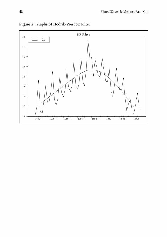
Fikret Dülger & Mehmet Fatih Cin48

Figure 2: Graphs of Hodrik-Prescott Filter

HP Filter2.6

2.4

2.2

2.0

1.8

1.6

1.4

1.2

1.01988 1990 1992 1994 1996 19981986 2000

V2PV2


ISSN 1301-1642 © ISE 1997

GLOBAL CAPITAL MARKETS

After a strong economic activity in the first quarter of 2002, concerns

increased about the pace and sustainability of a recovery. This was due to

downward revision of profit forecasts; concerns about the recovery has slowed

down and the leading indicators–while still stronger than at end-2001 -have

declined, except in emerging markets in Asia. The upturn in the United States

is now expected to be weaker than earlier as the GDP growth in 2002 is pulled

down significantly. In the euro area, domestic demand growth is likely to

increase slower than previously expected. In Japan, where the economy appears

to have bottomed out, GDP growth has been revised upward in both 2002 and

2003. However, with final domestic demand still weak, there are downside

risks to the outlook given the appreciation of the Yen. In Latin America, the

outlook has seriously deteriorated and output is expected to decline in 2002.

In emerging markets in Asia, the recovery has so far proved stronger than

expected, driven by the rebound in global trade and a nascent recovery in

information technology, and in some countries– notably China, India, and

Korea domestic demand. In the Middle East, while the outlook for oil prices

is somewhat stronger, the forecast has remained broadly unchanged. The global

growth is projected at 2.8 percent in 2002. Global financial markets have also

weakened. Industrial country equity markets have fallen sharply since end-

March. Equity markets in most emerging markets have descended over recent

months, although developments in foreign exchange markets have been

mixed.elmeimlaeimlaieklieThe performances of some developed stock markets with respect to

indices indicated that Nikkei-225 -100 increased by 12.2 %, DJIA, FTSE and

GDAX decreased by –9.6 %, -11.7 % and –11.7 %, respectively at the end

of June 2002 in comparison with the beginning of 2002. When US$ based

returns of some emerging markets are compared in the same period, the best

performer markets were: Indonesia (41.6 %), Thailand (38.3 %), Russia (38.1

%), Czech Rep. (20.2 %), S. Korea (19.1 %), S. Africa (16.6 %) and Hungary

(14.8 %). In the same period, the lowest return markets were: Argentina (-64.6

%), Turkey (-41.3 %), Brazil (-36.9 %), Venezuela (-34.8 %) and Israel (-

28.2 %). The performances of emerging markets with respect to P/E ratios as

of end-June 2002 indicated that the highest rates were obtained in Korea (43.6),

Malaysia (40.7), Philippines (33.6), Indonesia (30.7), Taiwan (25.4) and Turkey

(24.9), and the lowest rates in Argentina (-9.1), Poland (6.0), Brazil (9.7) and

Czech Rep. (10.1).

ISE Review50

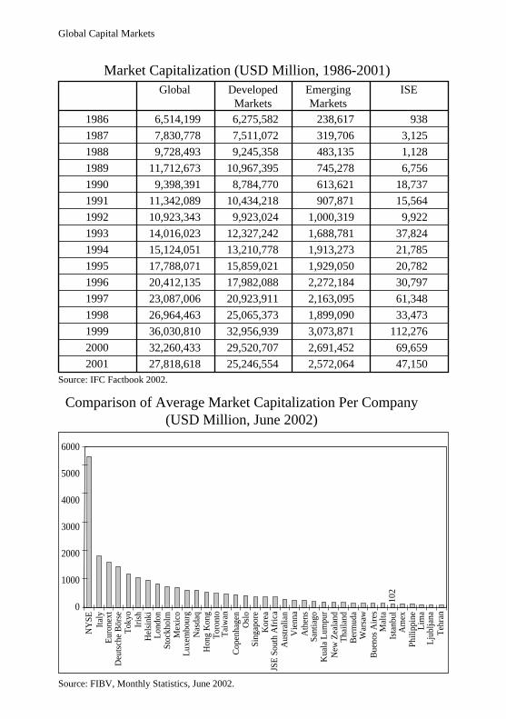
6,514,199

7,830,778

9,728,493

11,712,673

9,398,391

11,342,089

10,923,343

14,016,023

15,124,051

17,788,071

20,412,135

23,087,006

26,964,463

36,030,810

32,260,433

27,818,618

6,275,582

7,511,072

9,245,358

10,967,395

8,784,770

10,434,218

9,923,024

12,327,242

13,210,778

15,859,021

17,982,088

20,923,911

25,065,373

32,956,939

29,520,707

25,246,554

238,617

319,706

483,135

745,278

613,621

907,871

1,000,319

1,688,781

1,913,273

1,929,050

2,272,184

2,163,095

1,899,090

3,073,871

2,691,452

2,572,064

938

3,125

1,128

6,756

18,737

15,564

9,922

37,824

21,785

20,782

30,797

61,348

33,473

112,276

69,659

47,150

NY

SE

Ital

yE

uron

ext

Deu

tsch

e B

örse

Tok

yoIr

ish

Hel

sink

iL

ondo

nS

tock

holm

Mex

ico

Lux

embo

urg

Nas

daq

Hon

g K

ong

Tor

onto

Tai

wan

Cop

enha

gen

Osl

oS

inga

pore

Kor

eaJS

E S

outh

Afr

ica

Aus

tral

ian

Vie

nna

Ath

ens

San

tiag

oK

uala

Lum

pur

New

Zea

land

Tha

ilan

dB

erm

uda

War

saw

Bue

nos

Air

esM

alta

Ista

nbul

Am

exP

hili

ppin

eL

ima

Lju

blja

naT

ehra

n


Market Capitalization (USD Million, 1986-2001)

Comparison of Average Market Capitalization Per Company(USD Million, June 2002)

Source: FIBV, Monthly Statistics, June 2002.

Source: IFC Factbook 2002.

Global Developed Markets

EmergingMarkets

ISE

1986

1987

1988

1989

1990

1991

1992

1993

1994

1995

1996

1997

1998

1999

2000

2001

6000

5000

4000

3000

2000

1000

0

102

Worldwide Share of Emerging Capital Markets (1986-2001)

Share of ISE’s Market Capitalization in World Markets(1986-2001)

Source: IFC Factbook, 2002.

1986 1987 1988 1989 1990 1991 1992 1993 1994 1995 1996 1997 1998 1999 2000 2001

%60

%50

%40

%30

%20

%10

%0

Market Capitalization (%)

Trading Volume (%)

Number of Companies (%)


Share in Emerging Markets Share in Developed Markets

%4.0

%3.5

%3.0

%2.5

%2.0

%1.5

%1.0

%0.5

%0.0

%0.40

%0.35

%0.30

%0.25

%0.20

%0.15

%0.10

%0.05

%0.001986 1987 1988 1989 1990 1991 1992 1993 1994 1995 1996 1997 1998 1999 2000 2001

52 ISE Review

5,273,423

4,176,182

2,058,887

1,024,491

821,337

655,674

369,532

338,953

331,428

313,270

312,484

307,764

293,470

221,276

213,807

154,791

147,824

108,898

90,484

64,515

38,761

36,813

31,846

28,736

28,382

28,359

26,305

21,953

21,496

15,166

11,766

7,672

6,665

4,421

3,886

2,868

2,848

1,923

1,522

1,340

791

736

625

10,092,229

2,498,020

2,076,567

2,032,174

1,843,329

1,077,226

631,502

562,510

524,809

493,874

393,531

285,016

246,880

204,797

169,915

145,247

129,313

116,845

115,038

91,701

82,744

76,328

71,641

51,882

50,229

49,056

45,288

36,201

31,090

29,503

29,280

26,409

22,017

21,490

12,314

11,260

10,720

9,587

4,770

2,609

1,498

1,319

252

Main Indicators of Capital Markets (June 2002)

Market Value of Share Trading(Millions, US$)Up to Year Total(2002/1-2002/6)

Market Cap. of Share ofDomestic Companies

(Millions, US$)June 2002

Market

Source: FIBV. Monthly Statistics, June 2002

NYSE

Nasdaq

London

Euronext

Tokyo

Deutsche Börse

Taiwan

Korea

Spanish Exchanges

Amex

Swiss Exchanges

Italy

Chicago

Toronto

Bermuda

Stokholm

Australian

Hong Kong

Helsinki

Osaka

JSE South Africa

Singapore

Istanbul

Copenhagen

Sao Paulo

Oslo

Thailand

Mexico

Kuala Lumpur

Irish

Athens

Jakarta

Tel-Aviv

Warsaw

New Zealand

Budapest

Vienna

Philippine

Santiago

TSX Venture

Buenos Aires

Tehran

Ljubljana

1

2

3

4

5

6

7

8

9

10

11

12

13

14

15

16

17

18

19

20

21

22

23

24

25

26

27

28

29

30

31

32

33

34

35

36

37

38

39

40

41

42

43

NYSE

Tokyo

Nasdaq

London

Euronext

Deutsche Börse

Toronto

Swiss Exchanges

Italy

Hong Kong

Australian

Taiwan

Korea

Stockholm

JSE South Africa

Helsinki

Kuala Lumpur

Singapore

Mexico

Copenhagen

Athens

Oslo

Irish

Amex

Thailand

Santiago

Tel-Aviv

Jakarta

Istanbul

Vienna

Luxembourg

Warsaw

Philippine

New Zealand

Bounes Aires

Budapest

Lima

Tehran

Ljubljana

Bermuda

Colombo

Malta

Chicago

53Global Capital Markets

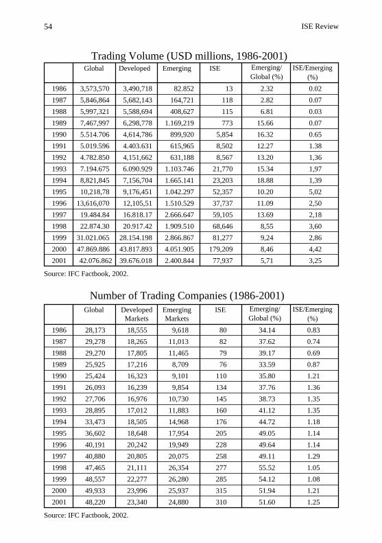
34.14

37.62

39.17

33.59

35.80

37.76

38.73

41.12

44.72

49.05

49.64

49.11

55.52

54.12

51.94

51.60

0.83

0.74

0.69

0.87

1.21

1.36

1.35

1.35

1.18

1.14

1.14

1.29

1.05

1.08

1.21

1.25

28,173

29,278

29,270

25,925

25,424

26,093

27,706

28,895

33,473

36,602

40,191

40,880

47,465

48,557

49,933

48,220

18,555

18,265

17,805

17,216

16,323

16,239

16,976

17,012

18,505

18,648

20,242

20,805

21,111

22,277

23,996

23,340

9,618

11,013

11,465

8,709

9,101

9,854

10,730

11,883

14,968

17,954

19,949

20,075

26,354

26,280

25,937

24,880

80

82

79

76

110

134

145

160

176

205

228

258

277

285

315

310

3,573,570

5,846,864

5,997,321

7,467,997

5.514.706

5.019.596

4.782.850

7.194.675

8,821,845

10,218,78

13,616,070

19.484.84

22.874.30

31.021.065

47.869.886

42.076.862

3,490,718

5,682,143

5,588,694

6,298,778

4,614,786

4.403.631

4,151,662

6.090.929

7,156,704

9,176,451

12,105,51

16.818.17

20.917.42

28.154.198

43.817.893

39.676.018

82.852

164,721

408,627

1.169,219

899,920

615,965

631,188

1.103.746

1.665.141

1.042.297

1.510.529

2.666.647

1.909.510

2.866.867

4.051.905

2.400.844

13

118

115

773

5,854

8,502

8,567

21,770

23,203

52,357

37,737

59,105

68,646

81,277

179,209

77,937

Trading Volume (USD millions, 1986-2001)Global Developed Emerging ISE

1986

1987

1988

1989

1990

1991

1992

1993

1994

1995

1996

1997

1998

1999

2000

2001

Emerging/

Global (%)ISE/Emerging

(%)


Number of Trading Companies (1986-2001)Global Developed

MarketsEmergingMarkets

ISE

1986

1987

1988

1989

1990

1991

1992

1993

1994

1995

1996

1997

1998

1999

2000

2001

Emerging/

Global (%)ISE/Emerging

(%)


54

2.32

2.82

6.81

15.66

16.32

12.27

13.20

15.34

18.88

10.20

11.09

13.69

8,55

9,24

8,46

5,71

0.02

0.07

0.03

0.07

0.65

1.38

1,36

1,97

1,39

5,02

2,50

2,18

3,60

2,86

4,42

3,25

ISE Review

38.2

14.5

27.8

17.6

17.5

12.3

21.6

11.7

27.1

16.8

20.0

14.3

16.3

28.2

13.1

10.7

17.1

15.4

15.9

8.8

25.2

16.8

11.2

11.6

13.5

22.2

12.5

10.3

12.1

32.4

4.8

18.9

13.4

7.0

15.1

-11.3

17.0

13.5

-106.2

-47.1

21.1

23.9

15.0

10.7

10.1

21.7

-3.7

7.8

39.0

25.1

37.7

-14.8

18.2

22.0

-10.5

-27.7

-19.1

14.1

24.0

22.0

17.4

49.2

-14.5

33.8

293.3

11.7

31.8

21.0

14.3

14.8

-6.5

19.3

71.7

12.5

28.2

19.4

10.7

13.7

-12.4

15.2

38.4

8.9

17.1

5.6

13.3

12.3

-14.1

24.9

53.2

13.2

28.4

6.0

11.7

28.5

47.3

69.5

-9.1

9.7

17.8

10.1

13.0

13.3

30.7

43.6

40.7

14.2

33.6

6.0

13.3

25.4

15.9

24.9

41.9

12.6

20.0

18.8

52.4

39.7

28.9

25.1

43.5

19.4

38.8

31.5

17.3

34.7

27.5

36.3

17.7

13.1

21.4

16.3

-55.3

26.7

20.2

34.5

29.0

17.1

30.8

12.9

21.3

36.8

21.2

31.0

15.0

36.3

17.1

11.2

12.0

14.2

19.8

19.8

25.1

28.4

19.0

7.0

18.8

21.4

21.7

8.4

Comparison of P/E Ratios Performances2000/12 - 2002/6

Price-Earnings Ratios in Emerging Markets (1993-2002/6)

Argentina

Brazil

Chile

Czech Rep.

Hungary

India

Indonesia

Korea

Malaysia

Mexico

Philippines

Poland

S.Africa

Taiwan, China

Thailand

Turkey

Source: IFC Factbook, 2001; IFC, Monthly Review, June 2002.Note: Figures are taken from IFC Investable Index Profile.

1993 1994 1995 1996 1997 1998 1999 2000 2001 2002/6

55

Indonesia

Thailand

Czech Rep.

Korea

S.Africa

Hungary

Malaysia

India

Philippines

Taiwan

Poland

Mexico

Chile

Brazil

Turkey

Argentina

-50.0 50.0 150.0 250.0 350.0

Source: IFC Factbook 2001. IFC, Monthly Review, June 2002.

2 0 0 2 / 62 0 0 12 0 0 0


1.6

0.7

1.6

0.9

2.0

2.1

2.7

0.8

3.8

1.7

3.1

2.6

2.3

3.3

1.8

4.0

1.8

1.1

1.6

0.8

3.7

2.7

1.5

0.6

1.8

2.5

1.7

1.6

1.9

3.8

0.8

9.2

1.3

0.6

1.1

0.7

3.2

1.9

1.6

0.9

1.3

1.4

1.3

1.5

1.5

2.6

1.2

2.7

1.5

1.6

1.8

1.2

3.6

3.1

2.9

2.0

1.9

2.2

1.5

2.0

2.7

3.3

2.6

8.8

1.0

1.4

1.5

1.2

2.5

2.5

1.6

0.8

1.5

1.7

1.2

2.2

2.1

1.7

1.6

3.1

0.6

1.2

1.4

0.8

1.8

2.0

1.9

1.3

1.3

1.7

1.1

1.4

2.1

2.1

1.6

3.8

1.0

1.2

1.3

0.8

1.7

2.3

1.3

1.4

1.5

1.7

1.1

1.4

2.0

1.9

1.9

2.4

1.9

0.5

2.1

1.3

1.6

4.9

3.1

1.4

5.4

2.6

5.2

5.7

1.8

3.9

4.7

7.2

1.4

0.6

2.5

1.0

1.7

4.2

2.4

1.6

3.8

2.2

4.5

2.3

2.6

4.4

3.7

6.3

1.3

0.5

2.1

0.9

1.2

2.3

2.3

1.3

3.3

1.7

3.2

1.3

2.5

2.7

3.3

2.7

IndonesiaThailand

RussiaCzech Rep.

KoreaS.AfricaHungaryMalaysia

ChinaSingapore

IndianPhilippines

Hong Kong

Egypt

TaiwanPoland

PeruMexico

Chile

VenezuelaIsrael

BrazilTurkey

Argentina

Comparison of Market Returns In USD(31/12/2001-3/7/2002)

Market Value/Book Value Ratios (1993-2002/6)

Source: : IFC Factbook, 1996-2001; IFC Monthly Review, June 2002.Note: Figures are taken from IFC Investable Index Profile.

-80 -40 -20 0 20 40 60-60

-64,6

-41,3

-36,9

-34,8

-28,2

-13,6

-8,7

-7,7

-7,2

-4,9

-3,5

-0,7

-0,6

0,3

1,8

5,5

6,2

14,8

16,6

19,1

20,2

38,1

38,3

41,6

Source: The Economist, July 6th-12th 2002.

Argentina

Brazil

Chile

Czech Rep.

Hungary

India

Indonesia

Korea

Malaysia

Mexico

Philippines

Poland

S.Africa

Taiwan, China

Thailand

Turkey

1993 1994 1995 1996 1997 1998 1999 2000 2001 2002/6

56 ISE Review

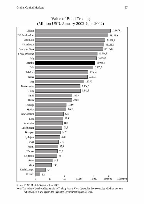
Source: FIBV, Monthly Statistics, June 2002.Note: The value of bonds trading pertain to Trading System View figures.For those countries which do not have

Trading System View figures, the Regulated Environment figures are used.

Value of Bond Trading (Million USD. January 2002-June 2002)

2,2

5,1

13,1

14,9

29,1

32,6

35,6

37,1

46,8

51,7

66,5

68,8

78,4

82,3

124,9

132,0

292,8

300,5

1.141,3

1.164,3

1.925,3

3.551,3

3.751,4

8.605,7

11.036,2

14,226,7

15.816,8

37.175,6

45.156,1

54.261,9

83.125,9

128.079,1

1 10 100 1.000 10.000 100.000 1.000.000

JSE South Africa

London

Stockholm

Copenhagen

Deutsche Börse

Swiss Exchange

Italy

Istanbul

Oslo

Tel-Aviv

Korea

Irish

Buenos Aires

Tokyo

NYSE

Osaka

Santiago

Mexico

New Zealand

Lima

Australian

Luxembourg

Budapest

Ljubljana

Taiwan

Vienna

Warsaw

Singapore

Amex

Malta

Kuala Lumpur

Helsinki

57Global Capital Markets

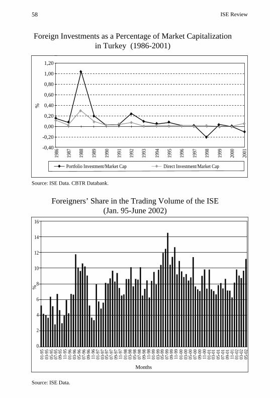
16

14

12

10

8

6

4

2

0

Source: ISE Data. CBTR Databank.

Foreigners’ Share in the Trading Volume of the ISE (Jan. 95-June 2002)

Foreign Investments as a Percentage of Market Capitalization in Turkey (1986-2001)

1,20

1,00

0,80

0,60

0,40

0,20

0,00

-0,20

-0,40

%

1986

1987

1988

1989

1990

1991

1992

1993

1994

1995

1996

1997

1998

1999

2000

2001

Source: ISE Data.

%

Direct Investment/Market CapPortfolio Investment/Market Cap

01-9

503

-95

05-9

507

-95

09-9

511

-95

01-9

603

-96

05-9

607

-96

09-9

611

-96

01-9

703

-97

05-9

707

-97

09-9

711

-97

01-9

803

-98

05-9

807

-98

09-9

811

-98

01-9

903

-99

05-9

907

-99

09-9

911

-99

01-0

003

-00

05-0

007

-00

09-0

011

-00

01-0

103

-01

05-0

107

-01

09-0

111

-01

01-0

203

-02

05-0

2

Months

58 ISE Review

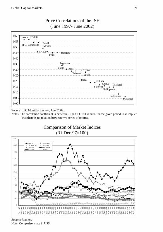
Price Correlations of the ISE (June 1997- June 2002)

Source : IFC Monthly Review, June 2002.Notes: The correlation coefficient is between -1 and +1. If it is zero. for the given period. It is implied

that there is no relation between two series of returns.

Comparison of Market Indices(31 Dec 97=100)

Source: Reuters.Note: Comparisons are in US$.

0,60

0,55

0,50

0,45

0,40

0,35

0,30

0,25

0,20

0,15

0,10

0,05

0,00

500

450

400

350

300

250

200

150

100

50

0

KOREA

SINGAPORE

RUSSIA

GREECE

PORTUGAL

AUSTRIA

MALAYSIA

TURKEY

Dec

. - 9

7Ja

n. -

98

Feb

. - 9

8M

ar. -

98

Apr

. - 9

8M

ay. -

98

June

- 9

8Ju

ly -

98

Aug

. - 9

8S

ep. -

98

Oct

. - 9

8N

ov. -

98

Dec

. - 9

8Ja

n. -

99

Feb

. - 9

9M

ar. -

99

Apr

. - 9

9M

ay. -

99

June

- 9

9Ju

ly -

99

Aug

. - 9

9S

ep. -

99

Oct

. - 9

9N

ov. -

99

Dec

. - 9

9Ja

n. -

00

Feb

. - 0

0M

ar. -

00

Apr

. - 0

0M

ay. -

00

June

- 0

0Ju

ly -

00

Aug

. - 0

0S

ep. -

00

Oct

. - 0

0N

ov. -

00

Dec

. - 0

0Ja

n. -

01

Feb

. - 0

1M

ar. -

01

Apr

. - 0

1M

ay. -

01

June

- 0

1Ju

ly -

01

Aug

. - 0

1S

ep. -

01

Oct

. - 0

1N

ov. -

01

Dec

. - 0

1Ja

n. -

02

Feb

. - 0

2M

ar. -

02

Apr

. - 0

2M

ay. -

02

June

- 0

2

59

Russia FT-100

IFCI CompositeBrazilMexico

S&P 500

ChileHungary

Argentina

Poland ‹srael S. AfricaTaiwan

Egypt

India Nikkei

S.KoreaChina

Philippines

Thailand

IndonesiaMalaysia



ISSN 1301-1642 © ISE 1997

ISEMarket Indicators

Num

ber

ofC

ompa

nies Total Daily Average

Traded Value Market Value P/E Ratios

1986

1987

1988

1989

1990

1991

1992

1993

1994

1995

1996

1997

1998

1999

2000

2001

2002

2002/Ç1

2002/Ç2

80

82

79

76

110

134

145

180

176

205

228

258

277

285

315

310

306

309

306

DividendYield

STOCK MARKET

Q: QuarterNote:* Between 1986-1992, the price earnings ratios were calculated on the basis of the companies’ previous year-end net

profits. As from 1993.TL(1) = Total market capitalization / Sum of last two six-month profitsTL(12) = Total market capitalization / Sum of last four three-month profitsUS$ = US$ based total market capitalization / Sum of last four US$ based three-month profits.

(TL Billion) (US$ Billion) (TL Billion) (US$ Billion)

(TL Billion) (US$ Billion)

(%) TL (1) TL (2) US$

9

105

149

1.736

15.313

35.487

56.339

255.222

650.864

2.374.055

3.031.185

9.048.721

18.029.967

36.877.335

111.165.396

93.118.834

43.527.477

24.857.113

18.670.364

13

118

115

773

5.854

8.502

8.567

21.720

23.203

52.357

37.737

58.104

70.396

84.034

181.934

80.400

31.904

18.382

13.522

—

—

1

7

62

144

224

1.037

2.573

9.458

12.272

35.908

72.701

156.260

451.892

375.479

351.028

414.285

291.724

—

—

—

3

24

34

34

88

92

209

153

231

284

356

740

324

257

306

211

709

3.182

2.048

15.553

55.238

78.907

84.809

546.316

836.118

1.264.998

3.275.038

12.654.308

10.611.820

61.137.073

46.692.373

68.603.041

49.293.803

57.824.887

49.293.803

938

3.125

1.128

6.756

18.737

15.564

9.922

37.824

21.785

20.782

30.797

61.879

33.975

114.271

69.507

47.689

31.436

43.254

31.436

9,15

2,82

10,48

3,44

2,62

3,95

6,43

1,65

2,78

3,56

2,87

1,56

3,37

0,72

1,29

0,95

1,27

1,26

1,27

5,07

15,86

4,97

15,74

23,97

15,88

11,39

25,75

24,83

9,23

12,15

24,39

8,84

37,52

16,82

108,33

—

93,13

—

—

—

—

—

—

—

—

20,72

16,70

7,67

10,86

19,45

8,11

34,08

16,11

824,42

—

108,29

—

—

—

—

—

—

—

—

14,86

10,97

5,48

7,72

13,28

6,36

24,95

14,05

411,64

—

100,57

—

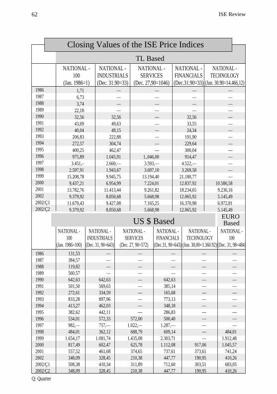
62 ISE Review

NATIONAL -100

(Jan. 1986=1)

NATIONAL -INDUSTRIALS(Dec. 31.90=33)

NATIONAL - SERVICES

(Dec. 27,90=1046)

NATIONAL -FINANCIALS(Dec.31.90=33)

NATIONAL -TECHNOLOGY

(Jun. 30.90=14.466,12)198619871988198919901991199219931994199519961997199819992000200120022002/Ç12002/Ç2

1,716,733,74

22,1832,5643,6940,04

206,83272,57400,25975,893.451,–

2.597,9115.208,78

9,437,2113.782,76

9.379,9211.679,43

9.379,92

————

32,5649,6349,15

222,88304,74462,47

1.045,912.660,—1.943,679.945,756.954,99

11.413,448.850,689.427,088.850,68

——————————

1.,046,003.593,—3.697,10

13.194,407.224,019.261,825.668,987.165,255.668,98

————

32,5633,5524,34

191,90229,64300,04914,47

4.522,—3.269,58

21.180,7712.837,9218.234,6512.065,9216.370,9812.065,92

——————————————

10.586,589.236,165.145,496.972,815.145,49

NATIONAL -100

(Jan. 1986=100)

NATIONAL -INDUSTRIALS

(Dec. 31, 90=643)

NATIONAL - SERVICES

(Dec. 27, 90=572)

NATIONAL -FINANCIALS

(Dec.31, 90=643)

NATIONAL -TECHNOLOGY

(Jun. 30,00=1.360.92)

198619871988198919901991199219931994199519961997199819992000200120022002/Ç12002/Ç2

NATIONAL -100

(Dec. 31, 98=484)

131,53 384,57 119,82 560,57 642,63 501,50272,61833,28413,27382,62534,01982,—484,01

1.654,17817,49557,52348,09508,38348,09

————

642,63569,63334,59897,96462,03442,11572,33757,—362,12

1.081,74602,47461,68328,45410,34328,45

——————————

572,001.022,—

688,791.435,08

625,78374,65210,38311,89210,38

————

642,63385,14165,68773,13 348,18 286,83500,40

1.287,—609,14

2.303,711.112,08

737,61447,77712,60447,77

——————————————

917,06373,61190,95303,51190,95

————————————

484,011.912,481.045,57

741,24410,26683,05410,26

US $ BasedEURO Based

Q: Quarter

TL Based

Closing Values of the ISE Price Indices

Q: Quarter(*) The Second quarter includes April-June period

Total Daily Average

1991

1992

1993

1994

1995

1996

1997

1998

1999

2000

2001

2002

2002/Ç1

2002/Ç2

1.476

17.977

122.858

269.992

739.942

2.710.973

5.503.632

17.995.993

35.430.078

166.336.480

39.776.813

39.827.440

14.192.919

25.634.521

BONDS AND BILLS MARKET

Traded Value

Outright Purchases and Sales Market

312

2.406

10.728

8.832

16.509

32.737

35.472

68.399

83.842

262.941

37.297

28.887

10.478

18.409

11

72

499

1.067

2.936

10.758

21.840

71.984

142.863

662.695

159.107

318.620

232.671

400.539

2

10

44

35

66

130

141

274

338

1.048

149

231

172

288

Total Daily Average

1993

1994

1995

1996

1997

1998

1999

2000

2001

2002

20021/Ç1

2001/Ç2

59.009

756.683

5.781.776

18.340.459

58.192.071

97.278.476

250.723.656

554.121.078

696.338.553

269.506.826

112.784.853

156.721.973

Repo-Reverse Repo Market

22

94

489

879

1.486

1.489

2.376

3.533

2.499

1.548

1.365

1.722

Repo-Reverse Repo Market

4.794

23.704

123.254

221.405

374.384

372.201

589.267

886.732

627.244

193.476

83.282

110.194

276

2.991

22.944

72.780

230.921

389.114

1.010.982

2.207.654

2.774.257

2.156.055

1.848.932

2.448.781

( TL Billion) ( US$ Billion) ( TL Billion) ( US$ Billion)

( TL Billion) ( US$ Billion) ( TL Billion) ( US$ Billion)

63ISE Market Indicators

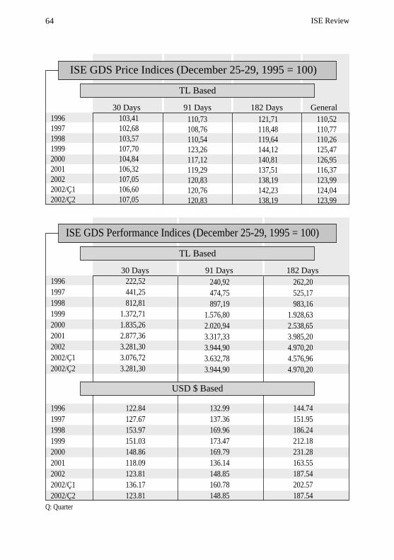
64 ISE Review

Q: Quarter

TL Based

19961997199819992000200120022002/Ç12002/Ç2

30 Days

ISE GDS Price Indices (December 25-29, 1995 = 100)

91 Days 182 Days General

1996

1997

1998

1999

2000

2001

2002

2002/Ç1

2002/Ç2

30 Days

ISE GDS Performance Indices (December 25-29, 1995 = 100)

91 Days 182 Days

TL Based

1996

1997

1998

1999

2000

2001

2002

2002/Ç1

2002/Ç2

USD $ Based

103,41102,68103,57107,70104,84106,32107,05106,60107,05

110,73108,76110,54123,26117,12119,29120,83120,76120,83

121,71118,48119,64144,12140,81137,51138,19142,23138,19

110,52110,77110,26125,47126,95116,37123,99124,04123,99

222,52

441,25

812,81

1.372,71

1.835,26

2.877,36

3.281,30

3.076,72

3.281,30

240,92

474,75

897,19

1.576,80

2.020,94

3.317,33

3.944,90

3.632,78

3.944,90

262,20

525,17

983,16

1.928,63

2.538,65

3.985,20

4.970,20

4.576,96

4.970,20

122.84

127.67

153.97

151.03

148.86

118.09

123.81

136.17

123.81

132.99

137.36

169.96

173.47

169.79

136.14

148.85

160.78

148.85

144.74

151.95

186.24

212.18

231.28

163.55

187.54

202.57

187.54

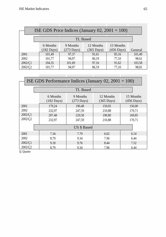
65

Q: Quarter

TL Based

200120022002/Ç12002/Ç2

6 Months(182 Days)

ISE GDS Price Indices (January 02, 2001 = 100)

General

200120022002/Ç12002/Ç2

ISE GDS Performance Indices (January 02, 2001 = 100)

TL Based

200120022002/Ç12002/Ç2

9 Months(273 Days)

12 Months(365 Days)

15 Months(456 Days)

6 Months(182 Days)

9 Months(273 Days)

12 Months(365 Days)

15 Months(456 Days)

US $ Based

101,49101,77104,35101,77

179,24

232,97

207,48

232,97

97,3794,97

101,6994,97

91,6186,1997,1686,19

85,1677,1091,6277,10

101,4998,61

103,5898,81

190,48

247,59

220,50

247,59

159,05

210,88

190,80

210,88

150,00

170,71

169,85

170,71

7.34

8.79

9.18

8.79

7.79

9.34

9.76

9.34

6.62

7.96

8.44

7.96

6.14

6.44

7.52

6.44

ISE Market Indicators

The purpose of this book is to help a wide range of investors use “open-

end” exchange traded funds (ETF’s) intelligently and effectively. The principle

objectives of this book are to help the reader to understand the reasons for ETF

growth and to use ETF’s profitably.

Chapter 1 focuses on the investor’s need for help on three topics that will

recur throughout the book: asset allocation and risk management, taxation and

financial planning and ETF selection and evaluation. Chapters 2, 3 and 4

attempt to answer how the ETFs work, why the expense ratios tend to be low

and how most of the funds manage to avoid significant capital gains distributions

and other frequently asked basic questions by the investors. ETF’s are also

compared with other basket products e.g. conventional mutual funds, that

often compete with them. Chapter 3 also cover the regulatory framework within

which the open ETF operates, introduce the transaction and tax cost allocation

functions of the in-kind fund share creation and redemption process and the

arbitrage pricing mechanism which prevents meaningful premium or discount

pricing of fund shares.

Chapter 5 provides ETF applications for investors and investment advisors.

Some illustrations and a frame of reference for present and prospective ETF

users are provided. Effective use of ETF’S will come naturally to investors

who recognize the fund as a portfolio, not just of stocks, but of risks and

rewards.

Chapter 6 addresses what has become the weak link in portfolio indexation:

the structure of common stock benchmark indexes and the way they are used

as templates for index funds. The indexes in use today have served relatively

well in the past, and their development have contributed significantly to the

growth of indexing, but there are signs of strain.

Chapter 7 explores the applicability of the ETF structure to fixed-income

funds and the possibility of actively managed ETFs. This chapter will help the

reader develop a greater understanding of the important features of existing

ETFs that will be used in the same way or in modified form in new types of

ETFs.

Kitap Tanitimi

“The Exchange Traded Funds Manual”, Gary L. Gastineau, John Wiley Sons

Ltd., New York, 2002, pp. xiii-401.


ISSN 1301-1642 © ISE 1997

Chapter 8 provides a schematic to illustrate the distinctive features of

liquidity, share trading characteristics, and market depth in exchange-traded

fund shares. Most fund share orders are executed promptly and fairly in a

highly liquid, highly transparent market; however there are important differences

between the market in ETF shares and the market in stocks.

A number of structural issues and obstacles to investment success and

the standard investment process practiced by experienced financial advisors

around the world as they attempt to develop financial and investment plans

for their clients and implement them in the form of specific portfolios are

described in chapter 9. It begins with thoughts on developing an appropriate

and useful relationship with an advisor.

ISE Review68

ISE REVIEW, Quarterly Economics and Finance Review published by the Istanbul Stock Exchange.

Starting with Volume 3 No: 10 issue (year 1999), full-text articles published in the ISE Review are now available through the Internet in pdf-format. Access to the printed version of the ISE Review for users with a fully paid subscription will be via an assigned password.

Abstracts:Abstracts of all articles published in the ISE Review are available through the ISE website. The database covers all abstracts of refereed journal articles published since 1997. Astracts df published articles are provided every three months, free of change, following the publication of the ISE Review.

Access: (1) http://www.ise.org/publictn.htm(2) select: ISE Review

For further information, comments and suggestions please contact:Tel: (90.212) 298 21 71 E-Mail: [email protected]

Now Online Access:

The ISE Review Subscription Order Form

Please check appropriate box for one year subscription.

US$ 30 for hard copy (4 issues no.22, 23, 24, 25) (US$ 7.5 per copy)

US$ 15 via E-Mail (4 issues no.22, 23, 24, 25) (US$ 3.75 per issue)

Name

Title

Company

Address

City State Zip

Phone Fax

E-Mail

Payment enclosed

Wire transfer to Türkiye ‹fl Bankas› Borsa Branch Account no: 1125 30103 4599

Please write the name of the publication and send us a copy

Please do not send cash

volume 6 no 22

Documents