Wars of Attrition with Evolving States

Germán Gieczewski∗

January 2017

Abstract

I study a model of wars of attrition with evolving states. Each player can choose

to continue the war or surrender; the game goes on until one player surrenders. The

bene�ts from each outcome, and/or the cost of waiting, are a function of the state of

the world. The state of the world is common knowledge and evolves slowly over time.

I show that, under general conditions, the game has a unique equilibrium in threshold

strategies, such that each player surrenders when the state is unfavorable enough to

her, and for intermediate states both players continue, until the war is resolved by the

evolution of the state. We then compare these results to existing variants of the war

of attrition. In an extension I �nd that, if one player has the option to make a partial

concession, this can give her a substantial advantage. Finally, I study the general game

where both players can make partial concessions.

PRELIMINARY AND INCOMPLETE.

1 Introduction

Dynamic wars of attrition are used to model a variety of phenomena in economics and

political science. Two �rms in a duopoly engaging in a price war; an activist group boycotting

a �rm; two countries, or two factions in a civil war, engaging in a protracted con�ict; an

army besieging a city, or two political parties drawing out a dispute over a policy can all

be understood as wars of attrition, among other examples. Previously, such models were

applied in biology to study animal con�icts (Smith, 1974). In these settings, we are often

interested in the answers to three questions. First, who is the most likely winner of the

war? Second, how much delay is there before the loser concedes or, in other words, how

∗Department of Politics, Princeton University.

1

much social welfare is lost? Third, how do these results vary as a function of the model's

parameters?

The simplest model of a war of attrition assumes that the payo�s from winning, as well as

the �ow costs of continuing the war, are common knowledge and �xed over time. Although

natural, these assumptions deliver unsatisfying results. As is known, this model has three

equilibria: two where one agent never surrenders while the other surrenders immediately, and

a third, mixed equilibrium where both players have a positive probability of winning, and

are always indi�erent between continuing or surrendering on the equilibrium path. In other

words, these equilibria give diametrically opposed predictions as to who will win and what

the expected delay is, making the model agnostic on the �rst two questions unless we take

a stand on equilibrium selection. If we were to choose an equilibrium that gives reasonable

answers�for instance, when the game is symmetric, both players should have equal chances

of winning�only the mixed equilibrium has any hope of yielding interesting answers. But,

as is also known, the mixed equilibrium has dysfunctional comparative statics: for instance,

when the bene�ts and costs are asymmetric, the weaker player (that is, the one with a higher

cost/bene�t ratio) is more likely to win. This occurs because, in a totally mixed equilibrium,

players must be indi�erent about surrendering at all times; if a player has high costs, giving

her enough incentives to ful�ll this condition requires the other player's surrender rate to be

high. In the limit, if one player has arbitrarily high �ow costs, she would be expected to win

almost surely. This is unreasonable: surely in this case it would be more sensible to simply

select the equilibrium where the high-cost player loses.

A more e�ective approach to this issue, which has also been used in related models of

bargaining (Abreu and Gul, 2000) and entry deterrence (Kreps and Wilson, 1982; Milgrom

and Roberts, 1982), is the introduction of behavioral or commitment types which add repu-

tational concerns to the game. In its simplest form, a war of attrition with reputation follows

the same rules as above, except that each player i has a small probability εi > 0 of being

a commitment type that never surrenders. As is known in this literature, even when the εi

are arbitrarily small, so that in all likelihood both players are rational, the temptation to

pretend to be a commitment type has a powerful e�ect on the equilibrium structure. In-

deed, the model with reputation has a unique equilibrium, which behaves more reasonably in

terms of comparative statics than the totally mixed equilibrium from the benchmark model.

In general, the higher-cost player has some probability of surrendering immediately, after

which the equilibrium path becomes totally mixed. However, this family of models has two

limitations. First, its predictions concerning the winner of the war are sensitive to the values

chosen for the εi: the player with a lower probability of being irrational is at a disadvantage

(and, in the limit, if a player is rational for sure she loses with certainty). This is somewhat

2

problematic if we take the εi as being not a true, measurable feature of real-world examples

but rather small perturbations used for equilibrium re�nement, as then there is little hope

of predicting a winner con�dently. Second, the elegance of this approach may wane in more

complicated games: for example, in bargaining applications where players can make di�erent

o�ers over time, it's no longer obvious what set of commitment types is appropriate, and

decisions regarding this may a�ect behavior on the equilibrium path.

In this paper, I develop a new model of dynamic wars of attrition that addresses these

concerns. In contrast with previous work, the model features an evolving state of the world

which is commonly observed. Concretely, costs are in�uenced by a one-dimensional param-

eter θt, which changes over time following a stochastic process. Intuitively, θt parameterizes

the extent to which current conditions in the war favor the �rst player over the second.

This device allows us to select a unique equilibrium despite the fact that there is complete

information on the equilibrium path; in particular, we do not rely on reputational concerns.

The selected equilibrium also has a novel structure, underlying intuition and implications:

when θt starts at an intermediate value, both players choose to continue the war initially,

and they have strict incentives to keep doing so. Eventually, when θt reaches an extreme

enough value, the player unfavored by the current conditions surrenders. (Of course, if θt

starts at an extreme value, the unfavored player surrenders immediately.) As a result, the

model predicts an equilibrium where both players have a positive probability of winning,

yet the equilibrium path is deterministic (except for the exogenous variation in θt) rather

than totally mixed, and both players obtain strictly positive payo�s from following their

strategies, compared to their utility from surrendering immediately.

I argue that the payo� perturbation driving the model can be interpreted in two ways.

On the one hand, it can be taken as a feature that re�ects a real phenomenon present in

practical examples: for example, the combatants in a war would know how the weather,

the state of their provisions, etc. is changing over time and how that a�ects their odds;

�rms in a price war would know how long they can a�ord to continue it for, given their

�nancial health. In this vein, a serious attempt at modeling wars of attrition including this

perturbation would entail estimating the process driving the underlying parameter θt, and

including that in the model. On the other hand, as often done in reputational models, the

changes in θt can be taken as a purely theoretical tool to obtain an equilibrium re�nement.

Under this interpretation, we are interested in the results of the limiting case as the rate of

change in θt goes to zero. I perform this exercise and obtain three interesting results. First,

the limiting model predicts a unique equilibrium for the unperturbed game, which�unlike the

case in reputational models�is independent of the speci�ed shape of the perturbations but

depends only on the fundamentals, i.e., the costs and bene�ts of each player. The predicted

3

equilibrium when the cost/bene�t ratios are di�erent is simple: the stronger player (that

with the lower ratio) wins immediately.1 But the predicted equilibrium in the symmetric

case is novel. The simplest way to describe it is to use tokens: essentially, it is as though

the players play a game in every turn, where the winner takes a token from the loser. If

one player runs out of tokens, she surrenders. This equilibrium gives both players the same

chance of winning, but it's not mixed and the players get strictly higher payo�s than in

the totally mixed equilibrium. Equivalently, the expected delay is lower than in the totally

mixed equilibrium, but it is guaranteed to be strictly positive.

Additionally, I study an extension of the model where one player has the option to make

a partial concession, lowering her own payo� but decreasing the other player's incentive to

continue the war. For example, a city under siege might give some of its wealth to the

attacking army to lower the expected value of looting the city if it is taken. This example

is interesting in its own right, but also serves to illustrate how the simplicity of model

can be leveraged to study more complex questions. I �nd that using this option can put

the conceding player at a great advantage: for example, in the limit case where the state

evolves very slowly, the conceding player can concede just enough to induce the opponent

to immediately surrender. Finally, I study the general game where both players can make

partial concessions over time.

This paper is connected to the existing literature on wars of attrition and bargaining.

Indeed, many papers have studied variants of the basic war of attrition involving a perturba-

tion. However, most of them have relied on various kinds of private information�generating

reputational concerns�rather than evolving payo�s to obtain their results. For example, ?

and Ponsati and Sákovics (1995) consider models where the players' bene�ts at the end of a

war depend on their types, which are private information. In Fudenberg and Tirole (1986)

and Egorov and Harstad (2017), it is the �ow costs of continuing the war which depend on

private types. Some of these models obtain a unique equilibrium while others still display

multiplicity, depending on further assumptions. The framework we take as a benchmark

for reputation-based perturbations is closest to Chatterjee and Samuelson (1987) and Abreu

and Gul (2000).

A few papers have employed modeling strategies closer to the one used here. Ortner

(2016) studies a game of bargaining with alternating o�ers where the bargaining protocol

(i.e., the identity of the player making o�ers) is driven by a Brownian motion. Ortner (2017)

considers two political parties bargaining in the shadow of an election; if an agreement is

reached, the result a�ects the relative popularity of the parties, which otherwise evolves

1This is also predicted by the model with reputation in the limiting case, but only if the εi are taken to

go to zero at a similar enough rate.

4

as a Brownian motion and eventually determines the outcome of the election. In Ortner

(2013), optimistic players bargain over a prize whose value changes over time. In Slantchev

(2003), players bargain using alternating o�ers while simultaneously �ghting; the course of

the war a�ects the o�ers that players will accept. In contrast, I assume that the changing

state of the world a�ects �ow costs, and use this perturbation to obtain a unique, intuitive

equilibrium in a model which otherwise displays equilibrium multiplicity�that is, the war of

attrition�rather than to alternating-o�ers bargaining.

The present paper also contributes to the literature on supermodular games started by

Topkis (1979) and Milgrom and Roberts (1990). Indeed, our modeling technique exploits the

fact that the war of attrition is a supermodular game when players' strategies are ordered in

opposite ways (i.e., player 1's �high� strategy is to continue while player 2's is to surrender);

and the fact that a perturbation produces equilibrium uniqueness is reminiscent of similar

contagion-based results in global games (e.g., Burdzy, Frankel and Pauzner (2001)).

The paper proceeds as follows. Section 2 presents the benchmark model, and Section 3

characterizes its equilibrium. Section 4 shows how the results translate to a continuous time

model. Section 5 takes the limit as the payo� perturbation becomes arbitrarily small, so

that the model converges to the basic war of attrition. Section 6 compares the predictions of

the model with those from the basic war of attrition and models with reputational concerns.

Section 7 discusses the case with partial concessions, and Section 8 concludes. All proofs

can be found in Appendix A.

2 The Model

There are two players, 1 and 2. For clarity, we �rst study a discrete-time model with in�nite

horizon: t = 0, 1, . . .. In each period, each player can choose to continue (C) or surrender

(S). There is a state of the world θt ∈ [−M,M ] which is common knowledge at all times.

Intuitively, θt represents how favorable the current conditions in the war are to either player:

a high θ favors 2, while a low θ favors 1. The initial θ0 is given by Nature.2 Then it evolves

according to a local Markov process, that is,

P (θt+1 − θt ≤ x|θt) = Hθt(x),

where Hθ is a distribution function with corresponding density hθ. Hθ has mean µ(θ) and

variance σ2. We assume that µ(θ) is continuous everywhere and weakly increasing for θ ∈2We take θ0 to be a �xed parameter. Assuming it to be random does not change the results, since it is

immediately revealed to both players.

5

[−M + δ,M − δ]; moreover, Hθ is weakly increasing in the same region in the FOSD sense.

Intuitively, this means that θ tends to drift to the extremes rather than to the middle. In

addition, Hθ has support [max(−δ, θ−M),min(δ,M − θ)] where δ > 0 is small. That is, Hθ

it has support [−δ, δ] except for the fact that θ can never leave the interval [−M,M ]. 3 The

simplest possible case, which we will use as a benchmark, is when h is symmetric around 0

and µ(θ) ≡ 0 for θ ∈ [−M + δ,M − δ].Payo�s are as follows. In any period where the war is ongoing and i chooses to continue,

she pays a �ow cost ci(θ). If the war has ended or i chooses to surrender, she pays no �ow

cost. When the war ends, the winner receives an instantaneous payo� Hi > 0 and the loser

receives Li, normalized to 0. If both players surrender on the same turn, the instantaneous

payo�s are split. For simplicity, there is no discounting,4 so that a i's lifetime payo� if the

war ends at time T is:

Ui = Hi1{i wins} −T−1∑t=0

ci(θt)− ci(θt)1{aiT=C}.

We assume that c1(θ) is strictly increasing in θ and c2(θ) is strictly decreasing in θ. Both

functions are di�erentiable. In addition, there are −M < −M1 < 0 < M2 < M such that

such that c1(−M1) = 0 and c2(M2) = 0. This assumption guarantees that player 1 will never

want to surrender when θ is below −M1, and 2 will never surrender above M2. Finally, we

assume that

c2(M1)M −M1 − δ

δ> H2

c1(M2)M −M2 − δ

δ> H1.

Intuitively, this means that M is large enough relative to M1 and M2 so that, if θ is very

close to M , player 2 will not surrender in the foreseeable future and hence it will be best for

player 1 to surrender, and vice versa.

3 Analysis

Given the above assumptions, there is a unique equilibrium, characterized as follows:

3In the continuous time limit of the model, θt follows a Brownian motion with drift µ(θ) and in�nitesimal

variance σ2, and has re�ecting boundaries at −M and M .4This does not lead to technical issues in terms of de�ning utility since it is never rational to continue the

war forever. At any rate, the results do not change qualitatively if a discount factor β close to 1 is included.

6

Proposition 1 (Equilibrium Characterization). There is a unique subgame perfect equilib-

rium (SPE) given by thresholds θ∗, θ∗, such that player 1 surrenders whenever θ > θ∗, player

2 surrenders whenever θ < θ∗, and neither player surrenders otherwise.

The intuition behind the solution is as follows. First, if θ is very low, then player 1 never

has a myopic incentive to surrender (i.e., even if she expected to eventually lose, she would

stay in the war until θ goes above −M1). Then, since the gap between −M1 and −M is

large, there will be low enough values of θ for which 2 is forced to surrender immediately, as

she understands that waiting for 1 to surrender will cost more than the rewards are worth.

Similarly, for very high θ, 1 must concede immediately. In other words, player 1 has two

dominance regions: one with low θ's that force her to continue and another with high θ's

that force her to surrender. The reverse is true for player 2.

For values of θ between these tentative thresholds, behavior will depend on expectations

about the other player's strategy. For instance, if 2 plays a �hawkish� strategy in equilibrium

(that is, she surrenders only for a small set of values of θ), this gives 1 incentives to play

a �dovish� strategy (which surrenders at a large set of values of θ) and vice versa. Since

the payo� of winning is worth waiting for a few periods, there must be a gap between the

surrender regions of both players. We call this intermediate region where both players �ght

the disputed region. Now consider a strategy pro�le where 1 is hawkish and 2 is dovish.

Intuitively, this is unstable because the disputed region would be an interval of high θ's,

where 2 has lower �ow costs than 1; therefore, if the disputed region is small, 2 would be

willing to expand it by reducing her surrender region; or, if the disputed region is large, 1

would want to shrink it by expanding her surrender region. The opposite problem occurs

if 1 is dovish and 2 is hawkish, so the thresholds θ∗, θ∗ delimiting the disputed region are

uniquely determined.5

We can interpret the values θ∗, θ∗ as parameterizing two features of the equilibrium. On

the one hand, the size of the disputed region, θ∗ − θ∗, re�ects how willing the players are to

�ght to increase their odds of winning the war, which is a function of the ratio between Hi

and the �ow costs of �ghting in the disputed region. In addition, if µ(θ) is increasing, this

tends to shrink the disputed region, as it leads an unfavorable θ to �snowball� and become

even more unfavorable over time, prompting a quicker surrender. On the other hand, the

position of the disputed region [θ∗, θ∗] within the interval [−M,M ] re�ects any asymmetries

between the players: if h and the �ow costs are symmetric then θ∗ + θ∗ = 0, while if µ > 0

(i.e., θ drifts to the right) or c1 > −c2 (i.e., 1 has higher costs) then θ∗ + θ∗ < 0 and so on.

We summarize these results in the following

5The formal proof also rules out cases where the surrender and disputed regions are not intervals.

7

Proposition 2 (Comparative Statics). The thresholds respond to changes in parameters like

so:

• Increases in H1 and decreases in c1 raise θ∗, θ∗ and θ∗ − θ∗. Increases in H2 and

decreases in c2 lower θ∗ and θ∗ but raise θ∗ − θ∗.

• If H1, H2 increase proportionally, θ∗ decreases and θ∗ increases.

• An increase in Hθ for all θ (in the FOSD sense) lowers θ∗ and θ∗.

4 Continuous Time Model

We now make an adjustment to the above game. Suppose that we split time into smaller

periods; in particular, the length of each period goes from 1 to κ2. The density of θ′ − θ|θis now given by 1

κhθ(xκ+ µ(θ)(1− κ)

), with mean µ(θ)κ2 and variance σ2κ2; and the �ow

costs are now ci(θ, κ) = ci(θ)κ2. These adjustments guarantee that the drift and variance

of the stochastic process, as well as the �ow costs, remain constant when measured by real

time. In the limit, the stochastic process governing θ converges to a Brownian motion with

local drift µ(θ) and local variance σ2. We then have the following

Proposition 3 (Continuous Time Equilibrium). Let θ∗(κ), θ∗(κ) be the equilibrium thresh-

olds from Proposition 1 as a function of κ. Then there are θ∗0, θ∗0 such that θ∗(κ) → θ∗0

and θ∗(κ)→ θ∗0 as κ→ 0.

In addition, each player's expected utility Ui(θ) and probability of winning Pi(θ), starting

at a given θ, can be calculated in [θ∗0, θ∗0] as the solution to the following ODEs:

U ′′i (θ) =2

µ(θ)2 + σ2(ci(θ)− µ(θ)U ′i(θ))

P ′′i (θ) = −2

µ(θ)2 + σ2µ(θ)P ′i (θ)

given the boundary conditions U1(θ∗0) = H1; U2(θ∗0) = 0; U1(θ∗0) = 0; U2(θ

∗0) = H2;

P1(θ∗0) = 1; P2(θ∗0) = 0; P1(θ∗0) = 0; P2(θ

∗0) = 1.

In particular, when µ ≡ 0, the solution in [θ∗0, θ∗0] reduces to

U1(θ) =2

σ2

∫ θ∗0

θ

(∫ θ∗0

λ

c1(ω)dω

)dλ =

2

σ2

∫ θ∗0

θ

(λ− θ)c1(λ)dλ P1(θ) =θ∗0 − θθ∗0 − θ∗0

U2(θ) =2

σ2

∫ θ

θ∗0

(∫ λ

θ∗0

c2(ω)dω

)dλ =

2

σ2

∫ θ

θ∗0

(θ − λ)c2(λ)dλ P2(θ) =θ − θ∗0θ∗0 − θ∗0

,

8

and the thresholds θ∗0, θ∗0 are determined by the conditions U1(θ∗0) = H1, U2(θ

∗0) = H2.

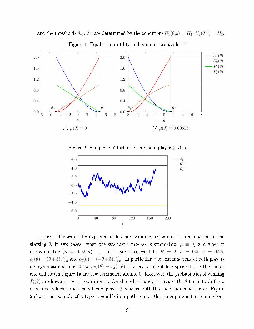
Figure 1: Equilibrium utility and winning probabilities

−8 −6 −4 −2 0 2 4 6 80.0

0.4

0.8

1.2

1.6

2.0

θ∗θ∗

θ

(a) µ(θ) ≡ 0

−8 −6 −4 −2 0 2 4 6 80.0

0.4

0.8

1.2

1.6

2.0

θ∗θ∗

θ

U1(θ)

U2(θ)

P1(θ)

P2(θ)

(b) µ(θ) ≡ 0.00625

Figure 2: Sample equilibrium path where player 2 wins

0 40 80 120 160 200

−6.0

−4.0

−2.0

0.0

2.0

4.0

6.0

t

θtθ∗

θ∗

Figure 1 illustrates the expected utility and winning probabilities as a function of the

starting θ, in two cases: when the stochastic process is symmetric (µ ≡ 0) and when it

is asymmetric (µ ≡ 0.025κ). In both examples, we take H = 2, σ = 0.5, κ = 0.25,

c1(θ) = (θ+5) κ2

1000and c2(θ) = (−θ+5) κ2

1000. In particular, the cost functions of both players

are symmetric around 0, i.e., c1(θ) = c2(−θ). Hence, as might be expected, the thresholds

and utilities in Figure 1a are also symmetric around 0. Moreover, the probabilities of winning

Pi(θ) are linear as per Proposition 3. On the other hand, in Figure 1b, θ tends to drift up

over time, which structurally favors player 2, whence both thresholds are much lower. Figure

2 shows an example of a typical equilibrium path, under the same parameter assumptions

9

as Figure 1a and starting at θ0 = 0: the state of the world is initially between the two

thresholds, so both players continue the war until θ reaches one of them, in this case player

1's.

5 Equilibrium in the Limit

When applying the model, the above analysis is relevant if we consider the movement of θ

to be a signi�cant feature of the application. However, the model also admits being used

simply as an equilibrium selection tool when the �true� model the researcher is interested

in is the basic war of attrition without perturbations. In this interpretation, we must take

the limit of the solution as the movement of θ becomes arbitrarily slow. Formally, we apply

the same transformations as in the previous Section to the stochastic process: the density

of θ′ − θ|θ is now 1νhθ(xν+ µ(θ)(1− ν)

), with mean µ(θ)ν2 and variance σ2ν2; but the costs

are left unchanged, and we take the limit as ν → 0. In this case the fundamentals of the

game are no longer the same, as the movement of θ has been slowed relative to the size of

the �ow costs.

Naturally, the limit of the game as ν → 0 is simply the unperturbed war of attrition,

but taking the limit of the perturbed equilibria yields a uniquely selected equilibrium of the

basic game:

Proposition 4 (Equilibrium Selection with Slow-Moving Processes). Suppose H1 = H2 =

H.6 Let θl be such that c1(θl) = c2(θ

l). Suppose c′1(θl) = −c′2(θl). Let θ∗(ν), θ∗(ν) be the

thresholds of the equilibrium in Proposition 1 as a function of ν. Then θ∗(ν), θ∗(ν) → θl as

ν → 0.

Hence, if θ0 < θl the perturbed equilibria converge, as ν → 0, to an equilibrium of the

unperturbed game where 1 wins instantly. If θ0 > θl, then 2 wins instantly in the limit.

If θ0 = θl the perturbed equilibria converge to an equilibrium of the basic war of attrition

augmented with tokens. In the augmented game, players observe a payo�-irrelevant variable

φt that follows a random walk, starting at 0 and obeying φt+1 = φt + 1, φt+1 = φt − 1 with

probabilities 0.5, 0.5. The limiting equilibrium is described by a unique threshold K such that

1 surrenders at any history where φt ≥ K, and 2 surrenders whenever φt ≤ −K.

In this equilibrium, both players have probability 0.5 of winning ex ante, and there is

delay, but both players are strictly willing to �ght, and i's expected payo� ex ante is H4> 0.

In other words, as the perturbation vanishes, the model o�ers a stark prediction for what

equilibrium should be selected in the unperturbed game: if one player has a higher �ow

6This serves to simplify notation.

10

cost7 than the other, then the equilibrium where she always surrenders immediately, and

the other player is never expected to surrender, should be played. This is not surprising,

since the perturbed game has a unique equilibrium, and any family of unique equilibria

for the unperturbed game displaying the right comparative statics (i.e., higher-cost players

should be more likely to lose) must make this selection. More interestingly, though, the

symmetric equilibrium selected when costs are equal is not the totally mixed equilibrium

of the unperturbed game, and in fact is not an equilibrium of the unperturbed game, as it

requires a coordination mechanism. Indeed, the equilibrium is as if each player were initially

in possession of K tokens, and a stage game were played every period; both players would

have equal probability of winning in each stage game, and the loser would pay one token

to the winner. (In terms of the formal statement, φt +K is the amount of tokens held by

player 2 at time t.) Then the selected equilibrium prescribes that a player should surrender

whenever she runs out of tokens.

6 Discussion

In this Section we discuss the merits of the model's results and compare them to existing

models of wars of attrition, namely the basic unperturbed model and an alternative based

on reputational concerns. Although these alternatives are not novel, for completeness we

brie�y de�ne the models and state their basic results; the details are in Appendix A. We

focus on the continuous time versions of both models as the discrete time versions introduce

some technical complications which are not relevant to our purposes.8

6.1 Basic War of Attrition

The basic, unperturbed war of attrition corresponds to a special case of our model where

µ = σ = 0, i.e., θ is constant. Alternatively, we can take c1(θ) ≡ c1 and c2(θ) ≡ c2 to be �at.

The following Proposition summarizes its set of SPE:

Proposition 5 (Equilibria of the Basic War of Attrition). The basic war of attrition has

three SPE:

• An equilibrium where 1 surrenders at every history and 2 never surrenders.

7In general, since the bene�ts from winning may di�er, what matters is the cost-to-bene�t ratio.8Namely, the discrete time basic war of attrition has a partially mixed equilibrium in addition to the

totally mixed one, where players take turns mixing vs. continuing for sure; this equilibrium converges to

the totally mixed equilibrium in the continuous time limit. Similarly, the equilibrium of the war of attrition

with reputation involves alternation in mixing.

11

• The opposite equilibrium where 1 wins immediately.

• A totally mixed equilibrium where both players mix at every history, and i chooses

to surrender at a rate pi =cjH

at every t. Players are indi�erent about continuing.

Players' expected payo�s ex ante are 0. i's probability of winning is cici+cj

.

As noted in the Introduction, this model has two main shortcomings. First, it provides

no way to select an equilibrium from the options o�ered, which saps it of explanatory power

as the set of equilibria includes extremes where either player wins for sure. Second, the

mixed equilibrium seems reasonable in the symmetric case, but it clearly has dysfunctional

comparative statics away from it: indeed, a player's probability of winning increases with

her own cost, and in the limit where one player has much higher costs than the other, that

player wins almost surely. These results derive from the mechanics driving the equilibrium:

since both players must be indi�erent along the equilibrium path, if i has high costs, then

j must surrender at a high rate to keep i willing to continue with positive probability. This

has little to do with the natural intuition behind the game, namely, that if i knows j has

lower costs, she might conclude that she probably cannot convince j to concede, leading to

i's surrender.

The perturbed model overcomes these issues: the movement of θ results in a unique

equilibrium being selected. Moreover, changes in the players' costs are parameterized simply

by movements in θ, which change the payo�s and probabilities of winning in the natural

way, i.e., the player with higher costs is more likely to surrender sooner and vice versa.

In addition, the equilibrium selected by the perturbed game in the symmetric case (or,

away from the slow-movement limit, in other cases where the war continues for some time)

produces strictly better welfare than the totally mixed equilibrium of the basic game. As

per Proposition 4, the sum of the players' expected payo�s is H2, whence the expected delay

is H4c, versus a total payo� of 0 and expected delay H

2cin the totally mixed equilibrium. It

should be noted, though, that the equilibrium selected by the perturbed model requires a

coordination device, and if such devices are allowed then even more e�cient equilibria are

possible. Indeed, the most e�cient equilibrium possible would involve the players �ipping a

coin, with the loser of the coin �ip conceding immediately. This would generate a total payo�

of H with no delay. It is an interesting fact in its own right, though, that this equilibrium

cannot be selected by the perturbed model.

6.2 War of Attrition with Reputation

The war of attrition with reputation takes the basic war of attrition outlined above, but adds

for each player i a probability εi of being a commitment type that never surrenders. Types

12

are private information. The following Proposition characterizes the SPE of this game:

Proposition 6 (Equilibrium of the War of Attrition with Reputation). The war of attrition

with reputation has a unique SPE, characterized as follows. Let t∗i be the vanishing time of

player i, characterized by e−cjHt∗i = εi. If t∗i = t∗j , then we say the players are balanced. The

probability that i (rational or not) will continue up to time t is Qit = e−cjHt for t ≤ t∗i . The

mass of rational i's surviving up to time t is Pit = e−cjHt− ε. The surrender rate for rational

i's is pit =cjH

1

1−εecjH

t; in particular, rational players are always mixing. At time t∗i = t∗j , only

commitment types are left and there is no surrendering thereafter.

If t∗i < t∗j , we say that i is stronger than j. In this case, a mass of j's rational types of

size Pj0 = 1 − εj

ε

cicji

surrender immediately at t = 0; after that, the players are balanced and

the equilibrium continues as above. In this case, the probability of winning for i's and j's

rational types are

Wi = Pj0 +1− Pj01− εi

[ci

ci + cj

(1− e−

ci+cjH

t∗i

)− εi

(1− e−

ciHt∗i

)]≈ Pj0 + (1− Pj0)

cici + cj

,

Wj =1− Pj01− εj

cjci + cj

(1− e−

ci+cjH

t∗i

)− εj

1− εj

(1− e−

cjHt∗i

)≈ (1− Pj0)

cjci + cj

.

i's expected payo� is Pj0H; j's expected payo� is 0.

The mechanics behind the equilibrium are as follows. After t = 0, rational types must

be willing to mix, as contradictions arise in all other cases. As in the unperturbed model,

for i to be willing to mix, j must be surrendering continuously at a rate ciH

(this is j's

overall surrender rate regardless of her rationality, so j's rational types must be surrendering

more often than this value to maintain the correct average), and vice versa. At this rate,

the rational types of player i would all surrender by time t∗i . If these vanishing times were

unequal, and e.g. t∗i < t∗j , then j's rational types would surrender at time t∗i , which would

incentivize i's rational types in some interval [t∗i−ε, t∗i ] not to surrender, and so on. To preventthis, a mass of j's rational types surrender at the beginning so that in the continuation the

rational types of both players will extinguish themselves at the same time.

As in the unperturbed war of attrition, the higher-cost player fares better (in the sense

of surrendering less often) after t = 0. However, if j has a higher �ow cost, that also results

in a higher t∗j , and therefore a higher probability of surrendering immediately. Overall the

latter e�ect wins, so that having a higher �ow cost reduces a player's equilibrium payo�

and probability of winning. However, the vanishing times are also a function of the εi, so

guaranteeing that a certain relationship between �ow costs translates into a certain player

likely winning the war requires some assumption on these parameters. Speci�cally, if ci < cj,

13

then as εi, εj → 0 we have that Pj0 → 1, but only ifεcjj

εcii

→ 0. In other words, εi cannot be

going to 0 much faster than εj; otherwise, this e�ect would overrule the relationship between

the �ow costs and j would be favored to win the war. When applying the model, we might

be willing to assume that εi ≈ εj so that there is no issue, but if the ε's are expected to be

very small this assumption will be hard to verify or disprove based on any sort of data the

researcher has access to.

In this aspect, the model proposed in this paper appears more robust: if we are interested

in using the perturbation as an equilibrium selection tool, the results as ν → 0 do not depend

on the shape of the functions ci(θ) away from the θ0 we are focused on. They only depend

on (c1(θ0), c2(θ0)) as shown by Proposition 4, so long as the functions are continuous.

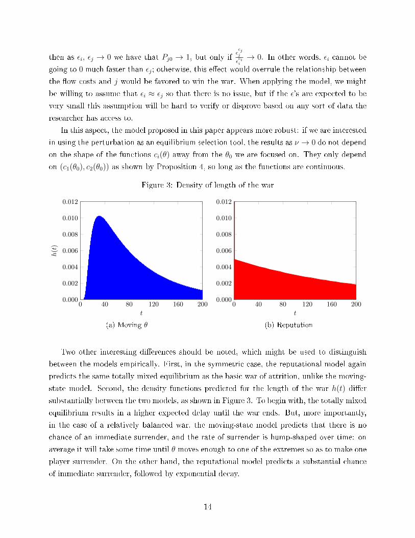
Figure 3: Density of length of the war

0 40 80 120 160 2000.000

0.002

0.004

0.006

0.008

0.010

0.012

t

h(t)

(a) Moving θ

0 40 80 120 160 2000.000

0.002

0.004

0.006

0.008

0.010

0.012

t

(b) Reputation

Two other interesting di�erences should be noted, which might be used to distinguish

between the models empirically. First, in the symmetric case, the reputational model again

predicts the same totally mixed equilibrium as the basic war of attrition, unlike the moving-

state model. Second, the density functions predicted for the length of the war h(t) di�er

substantially between the two models, as shown in Figure 3. To begin with, the totally mixed

equilibrium results in a higher expected delay until the war ends. But, more importantly,

in the case of a relatively balanced war, the moving-state model predicts that there is no

chance of an immediate surrender, and the rate of surrender is hump-shaped over time: on

average it will take some time until θ moves enough to one of the extremes so as to make one

player surrender. On the other hand, the reputational model predicts a substantial chance

of immediate surrender, followed by exponential decay.

14

7 Partial Concessions

We now extend the model to study the following variant of the war of attrition: as before,

players are able to continue the war until one surrenders, but while the war is ongoing they

can a�ect the payo�s of the eventual outcome by making partial concessions. For instance:

• An army sieges a city. The city has strong walls and cannot be taken by assault, so

a siege will lead to two outcomes: either the army surrenders (meaning it leaves with

nothing) or the city surrenders (meaning it opens its doors and the army plunders it).

In this example, movements in θ re�ect changes in the fortunes of each side: the city's

supplies may dwindle or they may be able to smuggle in fresh supplies, either side may

su�er a disease outbreak, and so on. Instead of surrendering outright, the city can

instead pay tribute to the army: that is, it can gather some wealth, give it to the army

and invite them to leave. If this tactic is successful, it is more e�cient for both sides,

since the city's gathering of its own wealth entails lower welfare losses (no buildings

are burned, no civilians are killed, and so on). There is no commitment device, so the

army can still stay to siege after receiving tribute. But the tactic may work because

the remaining loot to be had is smaller, while the city is still eager to defend itself

(since the deadweight loss from being plundered is large).

• A polluting �rm is boycotted by an activist group. The boycott is costly for both

players, as it lowers �rm sales and consumer surplus. The war ends when either the

�rm capitulates to the demands or the activists abandon the boycott. However, the

�rm may have access to a range of policies it can implement to lower its own pollution.

A partial concession, in the form of a moderate level of self-regulation, may be enough

to �de�ate� the momentum of the boycott even if it is not what the activists demanded.

Similar logic can apply to a government implementing emergency measures to appease

protesters.

The common theme in these examples is that making a partial concession may bene�t

the party who does it: although it entails giving up some payo�s, this is often worth it if it

will tilt the remaining war of attrition towards the side who partially concedes. We ask our

model to answer two main questions: when are partial concessions useful? (For instance, are

they only useful when they enable higher e�ciency than the noncooperative outcomes, as in

the siege example? Or can they be useful even when there is no e�ciency gain involved?)

And what is the optimal size and timing of a partial concession? We �rst study the case

where only player 1 can make partial concessions, and then the case where both players can.

In addition, we compare the results under two assumptions about timing: in one version, we

15

take concessions to be one-shot, i.e., there is a �xed time when a concession must be made,

or else the chance to do so is lost forever; in the other, multiple concessions can be made

whenever the player wants, subject only to the restriction that concessions cannot be taken

back.

One-Sided Concessions

The Limit Case

For simplicity and to �x ideas, we �rst discuss the limit case where ν ≈ 0. First, assume

a one-shot concession at the beginning of the game: player 1 chooses a concession size x at

t = 0. Thereafter, the game continues as usual, except that she gets H − αx from winning

compared to losing, while 2 gets H−x from winning. Here α represents the relative e�ciency

of the concession technology: if α < 1, a concession reduces 1's incentive to win the war

relatively less than 2's incentive, and vice versa.

Note that α < 1 (α > 1) does not necessarily imply that the concession generates

(destroys) social welfare, as payo�s may have been normalized di�erently for each player.

For instance, in the siege example, the bene�ts from winning before the concession would

be higher for the defender than the attacker, i.e., HD > HA, since a losing defender su�ers

the cost of being plundered which is not collected by the attacker; and there would be some

�ow costs cD, cA. A transfer x from D to A would change D's payo�s to HD−x for winning

or 0 from losing, while A's would change to HA or x, respectively, generating no net change

in welfare. However, if at the outset we had normalized the problem so that bene�ts were

equal for both sides, then we might have normalized payo�s H = H̃D = αHD = H̃A = HA;

c̃D = αcD; c̃A = cA; and a transfer of x would change the bene�ts of winning to H − αx for

D and H − x for A, where α = HA

HD.

Proposition 7 (One-Shot Concession with Slow-Moving θ). The equilibrium of the game is

as follows:

• If c1 < c2, player 1 makes no concessions and wins immediately.

• If c1 ≥ c2 and α < 1, player 1 makes a concession x∗ de�ned by:

H − αx∗c1

=H − x∗c2

and wins immediately. This leads to a concession x∗ = H c1−c2c1−αc2 , and payo�s U1 =

H − αH c1−c2c1−αc2 , U2 = H c1−c2

c1−αc2 .

16

• If α ≥ 1, concessions never bene�t player 1. Hence, if c1 = c2, no concession is made

(x∗ = 0) and the equilibrium described in Proposition 4 is played. If c1 ≥ c2, any

x∗ ∈ [0, H] is compatible with equilibrium but player 1 loses immediately in all cases.

In other words, when θ moves very slowly, partial concessions can be useful�but only

when they strengthen the conceding player's relative cost-bene�t ratio, i.e., when α < 1.

In this case they are very powerful, and indeed guarantee that player 1 always wins the

game in equilibrium, even when c1 is substantially higher than c2. Of course, this does not

necessarily mean that player 1 walks away with a large payo�, as the concession needed to

win may be large. In particular, the required concession H c1−c2c1−αc2 is small when α << 1

(so that player 1 only needs to take a small dent in her own payo� to substantially reduce

2's incentive to win), or when c1 and c2 are close (so 1 is not very disadvantaged to begin

with, so a small nudge is enough to make 2 surrender). Conversely, as α→ 1, if c1 > c2 the

required concession converges to H.

On the other hand, when α ≥ 1�that is, when a concession weakens 1's relative cost-

bene�t ratio�making a concession can never help player 1. This seems like a natural result,

although we will see that matters are subtler away from the limit case.

Finally, note that in the limit case the timing of concessions actually does not matter:

although we have stated the above result in a game where 1 can only make a concession at

t = 0, the equilibrium is trivially the same if 1 is instead allowed to make multiple concessions

at any time. Indeed, if α < 1 or c1 < c2, so that 1 is able to win in equilibrium, she might

as well make the winning concession immediately, so as to avoid any cost of waiting.

7.0.1 General Processes

We limit ourselves here to the case of one-shot concessions:

Proposition 8 (Equilibrium with a One-Shot Concession). The equilibrium of the game is

as follows:

• If θ < θ∗, player 1 makes no concession and wins immediately.

• If θ ≥ θ∗, let (θ∗(x), θ∗(x)) be the thresholds resulting in the continuation game after a

concession of size x is made. Let x1 be the smallest concession for which θ∗(x) ≥ θ, i.e.,

player 1 wins immediately in the continuation (we take x1 = ∞ if no x satis�es this

requirement). Let x2 ∈ [0, x1] be a minimal concession that maximizes 1's surrender

threshold, i.e.,

x2 = min(argmaxx∈[0,x1]θ

∗(x)).

17

Then x2 is the optimal concession. Moreover, θ∗(x) is quasiconvex, so either x2 = 0

or x2 = x1. In the �rst case, no concession is made; in the second, player 1 wins

immediately.

In particular, keeping all other parameters �xed, there is α∗ < 1 such that for all α ≥ α∗

it is optimal to choose x∗ = 0, while for α < α∗ the optimal choice is x∗ = x2. In addition,

player 1's equilibrium utility is decreasing in α.

The intuition behind this result is as follows. By Proposition 3, as long as θ is far from

the surrender thresholds, a concession which lowers 1's potential payo� from winning�while

also changing the surrender thresholds�actually has no impact on her expected utility except

by changing said thresholds. This follows immediately from the fact that H does not feature

in the expression for expected utility. Moreover, this expression is clearly increasing in

θ∗, whence 1 e�ectively wants to maximize her own surrender threshold. Two surprising

implications follow.

First, the optimal concession may not be one that results in an immediate win for player

1: indeed, she may choose to make a positive concession which still leaves the outcome of

the war in doubt, and produces delay.

Second, whenever α > 1 concessions always hurt player 1, but this is also true for some

values of α that are below 1. The intuition behind this result is that there are two forces which

a�ect the surrender thresholds when x changes, as anticipated in Proposition 2. On the one

hand, a higher x reduces the stakes of winning for both players; this reduces their willingness

to accept delay, so it tends to bring both thresholds closer to each other while having no clear

impact on their average. On the other hand, if α < 1 (> 1) the concession tends to increase

(decrease) both thresholds and as it strengthens (weakens) player 1's relative strength. For

a positive concession to be optimal, there must be a range of concession values for which the

latter e�ect dominates the former, which requires α to be below 1 by a certain amount. Note

that, in particular, this means that player 1 may decline to make a concession even when

this might guarantee a win for a small cost: for example, if α = 1 and θ is initially close

to θ∗(0), a small concession might be enough to bring θ∗(x) up to θ, clinching the win; but,

since this would also decrease θ∗, it follows that the cost of the concession is higher than the

gains in terms of reduced delay and increased probability of winning.

Two-Sided Concessions

We now move on to a further extension where both players are able to make concessions.

This can be thought of as a form of bargaining by means of unilateral o�ers. To �x ideas,

consider the following examples:

18

• Two players, a buyer and a seller, engage in a war of attrition over the price at which

B might buy a good worth H. As the war continues, B can make statements of the

form: �I will buy for any price up to x�, while S can say, �I will sell for any prize above

y�. These promises are binding, so B's acceptable price xt cannot decrease over time

and vice versa. Whenever a player surrenders, the transaction happens at the price set

by the other player's most recent statement.

• Two armies contest a one-dimensional territory [0, 1], where vi(t) is the value assigned

to point t by player i, and Hi =∫ 1

0vi(t)dt. Assume v1 is decreasing and v2 is increasing.

While the war is ongoing, the armies station troops at outposts throughout the territory

to contest its control and engage in intermittent �ghting, generating �ow costs. Along

the way, each player i can make credible, irreversible commitments to pull her troops

out of a measurable region S ⊆ [0, 1]. When a player surrenders, she keeps only the

territory that the other player conceded, and the other player takes the rest.

As a reasonable compromise between generality and simplicity, we allow for each player i

to have a concession factor αi, so that if initial rewards from winning are Hi, Hj and i makes

a concession x, rewards become Hi − αix, Hj − x. In the bargaining example, we would

have α1 = α2 = 1, since concessions take the form of transfers. In the war for territory,

the αi would vary depending on the exact territory conceded, but at the margin we would

have α1α2 < 1: indeed, if i is trying to reduce j's incentives to �ght relative to her own, the

optimal strategy is to concede territory that j values most and i least, i.e., 1 would make

concessions of the form [t, 1] and 2 would make concessions of the form [0, t′], which result

in the conceding player's incentive to win going down less than the recipient's.

We will focus on the limit as ν → 0. We normalize the costs and bene�ts so that

c = c1 = c2 to streamline the notation. For clarity, we restrict the players to the following

concession protocol: at the beginning of the game, 1 chooses a partial concession, then 2

observes it and makes a partial concession of her own; then the rest of the game proceeds

as usual. (It can be shown that switching the order of concessions, adding more alternating

concessions, making them simultaneous or allowing concessions after t = 0 have no impact

on the equilibrium concessions and payo�s.)

Proposition 9 (Two-Sided Concessions with Slow-Moving Processes). The equilibrium of

the game is as follows. First, if α1 ≥ 1, α2 ≥ 1 then concessions are not used and the

equilibrium is as in Proposition 4. Similarly, if α1 < 1, α2 ≥ 1 then only player 1 may use

concessions and the equilibrium is as in Proposition 7. If α1 < 1, α2 < 1 then:

• If H1 < α1H2, player 2 wins immediately without making a concession and payo�s are

19

(U1, U2) = (0, H2).9

• If H2 < α2H1, player 1 wins immediately without making a concession and payo�s are

(U1, U2) = (H1, 0).

• Otherwise, both players make partial concessions x1 = H2−α2H1

1−α1α2, x2 = H1−α1H2

1−α1α2which

jointly exhaust the prize, and payo�s are

U1 =H1 − α1H2

1− α1α2

, U2 =H2 − α2H1

1− α1α2

.

The intuition behind the result is as follows. As before, a player can try to use a concession

to improve her relative strength and win the war. However, player 1 understands that making

a concession just large enough so that H1− α1x1 ≥ H2− x1, as she would do in Proposition

7, is not enough here because player 2 will undercut her with her own concession. Hence,

in equilibrium player 1 concedes enough so that player 2 cannot win except by conceding

the entirety of the remaining prize. The resulting payo�s turn out to be the same as when

player 2 concedes �rst and follows the same logic.

8 Conclusions

We have analyzed a model of wars of attrition with an evolving state of the world. As

intended, the perturbation used in the model yields several attractive properties which are

absent from the baseline model. In particular, the game has a unique equilibrium, yielding

predictions about the likely winner which re�ect a natural intuition about how this game

might play out in practice. Moreover, the solution exhibits well-behaved comparative statics,

meaning that if a player's bene�t from winning increases or her �ow cost decreases, she will

be more likely to win. In the same vein, such a change will lead to the war ending sooner if

the player being strengthened held an advantage to begin with, while the war will lengthen

if she was an underdog at �rst. These properties are shared by models based on reputational

perturbations, but unlike those, the present model is more robust to assumptions about how

the game looks away from the perturbation, an attractive property for applied researchers

who may not be able to observe enough detail about a real example to guarantee that they

are modeling perturbations correctly.

In addition, the present model is highly tractable, which allows it to be used as a modeling

tool in other settings or in applied problems. This is illustrated in Section 7, which shows how

9Technically there is a collection of equilibria giving the same outcome, as player 1 can make concessions

that have no impact on payo�s.

20

to account for the possibility of partial concessions during a war of attrition, and how access

to this option might bene�t the player making concessions. But many other applications are

possible: for instance, the game can be extended to explore the use of costly commitment

devices, i.e., �burning bridges�; to wars of attrition involving more than two players, as in

legislative stando�s; or to cases where players have some control over the �ow costs, such as

price wars.

Finally, the model makes a novel prediction regarding the most natural equilibrium in

balanced wars of attrition (where both players have similar chances of winning), which entails

higher payo�s than a totally mixed equilibrium, as well as a di�erent distribution for the

expected length of the war. This raises the question whether this equilibrium is indeed

played in real-life scenarios, or under what circumstances (e.g., does there have to be a

changing, publicly-observed variable which is focal for the players?), a question which might

be answered by laboratory or �eld experiments.

21

A Appendix

PRELIMINARY AND INCOMPLETE.

Proof of Proposition 1. First note that there are −M < M < −M0, M0 < M < M such

that, in any SPE, player 1 surrenders if θ > M and 2 surrenders if θ < M . The incentive for

1 to surrender stems from the fact that 2 never surrenders for any θ > M0. Then, if M −M0

is large enough, 1 knows that 2 will surrender with very small probability within the nextH−Lc

periods, so no continuation does better for 1 than to surrender immediately. The other

side is analogous.

Next, we argue that the game is supermodular in the following sense: take the partial

order on 1's strategies given by σ1 ≥ σ′1 i� σ1(h) ≥ σ′1(h) for all h (here σ1(h) is 1's surrender

probability after history h); and take the reverse order on 2's strategies, i.e., σ2 ≥ σ′2 i�

σ2(h) ≤ σ′2(h) for all h. Then, if σ1 ≥ σ′1, and given a strategy σ2 for 2, 2's continuation

payo� from not surrendering at any history h, and then following σ2, is higher when 1 is

playing strategy σ1 than when 1 is playing σ′1. In other words,

U2(NS, σ2, σ1|h) ≥ U2(NS, σ2, σ′1|h)

for all histories h. Analogously, if σ2 ≥ σ′2, then U1(NS, σ1, σ2|h) ≤ U2(NS, σ1, σ′2|h) for all

h. Since, in any SPE, a player must not surrender only if the expected continuation payo�

from not surrendering is positive, higher (less aggressive) strategies by 1 induce higher (more

aggressive) strategies by 2 and vice versa.

The proof is �nished in the standard way for supermodular games. First, we can show

the existence of a greatest and a lowest equilibrium, which can be obtaining by iterating the

best response correspondence starting from the pro�les σ0 = (1, ) and σ0 = (,1) respectively.

(Here 1(h) = 1 for all h and (h) = 0 for all h.)

Moreover, we can check that at every step the result of either iteration is a pro�le

(σ1k, σ2k) (or σk) given by threshold strategies. That is, there are θ∗k, θ∗k such that

σ1k(h) = 1{θ(h)>θ∗k and σ2k(h) = 1{θ(h)<θ∗k . This follows from a more general lemma:

Lemma 1. Let σ2 = 1{θ(h)<θ0 be a threshold strategy for player 2. Then there is θ′ such that

σ1 = 1{θ(h)>θ′ is the unique best response for 1.

Proof. Suppose σ1 is a best response to σ2. By our previous arguments, σ1(h) = 1 for θ > M .

Let σ̃1 be a strategy given by σ̃1(h) = 1{σ1(h)>0}, i.e., σ̃1 surrenders for sure whenever σ1

surrenders with positive probability. It is clear that U1(σ1, σ2) = U1(σ̃1, σ2), since 1 is

22

indi�erent about surrendering in all cases where the two strategies di�er. Next, let

θ′ = inf{θ ∈ [−M,M ] : σ̃1(θ′) = 1}.

We argue that σ̃1(θ) must equal 1 for all θ ∈ [θ′,M ]. Indeed, since 2 never surrenders in

[θ′,M ], any continuation of the game starting at a θ ∈ [θ′,M ] where 1 does not immediately

surrender will see him paying positive costs for a number of periods until he inevitably

reaches a θ′′ for which σ̃1(h) = 1 and surrenders, netting a negative payo�. Hence, if σ̃1 is a

best response to σ2, 1 must be surrendering immediately in [θ′,M ].

Next we show that the threshold θ′ is unique.

By construction, U1(θ) = H for θ ≤ θ0 and U1(θ) = 0 for θ ≥ θ′. Moreover, U1 is

decreasing in [θ0, θ′], since

U1(θ + ε) = −∑

{h:θ(h′)∈(θ,θ′) ∀h′⊆h}

p(h)c(θ(h)) + pU1(θ) < U1(θ),

where the sum runs over all histories starting from state θ + ε at t = 0 where θ has stayed

between θ and θ′, and p is the probability that θt reaches θ before reaching θ′. In addition,

by the optimality of σ1, it must be true that U1(θ′ − ε) > 0 but U1(NS, σ1, θ

′) < 0, i.e., 1's

utility at θ′ if he refuses to surrender but subsequently follows strategy σ1 is negative.

Now consider σ′1 = 1{θ(h)>θ′−ε. We argue that U1(σ1, σ2, θ) > U1(σ′1, σ2, θ) for all θ ∈

(θ0, θ′ − ε]. Indeed, this is true for θ = θ′ − ε by the previous observation. Then, it follows

for θ ∈ (θ0, θ′ − ε) because the �ow payo�s from both strategies are identical except for the

case where θ eventually reaches θ′ − ε before reaching θ0, in which case σ1 is superior.

By the same argument, the payo� from the strategy 1{θ(h)>θ′′ , starting at any θ ∈ (θ0, θ′),

is decreasing in θ′′ for all θ′′ < θ′. An analogous argument shows that increasing the threshold

beyond θ′ also leads to strictly worse payo�s.

Intuitively, if player 2 is surrendering whenever θ < θ∗, then 1's payo� from continuing

will be decreasing in θ, both because c(θ) is increasing in θ and because the expected time

until 2's surrender is increasing in θ.

Finally, note that σk must be decreasing in k and σk must be increasing in k, and their

limits must also be threshold strategy pro�les σ ≥ σ which are also SPEs. The last step is

to show that σ = σ.

Solution of a threshold equilibrium θ∗, θ∗:

prob of hitting lower threshold starting at θ is P (θ)

P (θ) = q(θ)P (θ + ε) + (1− q(θ))P (θ − ε)

23

So if the process is uniform, P is just linear! However, U will be convex due to the waiting

cost

Ui(θ) = q(θ)Ui(θ + ε) + (1− q(θ))Ui(θ − ε)− ci(θ)

We can solve from each extreme: let [θ∗, θ∗] ∼ {0, . . . , l}

0 = U2(0) =U2(1)

2− c2(0) ⇒ U2(1) = 2c2(0)

U2(1) =U2(2)

2− c2(1) ⇒ U2(2) = 2(U2(1) + c2(1)) = 2c2(1) + 4c2(0)

U2(2) =U2(3)

2+U2(1)

2− c2(2) ⇒ U2(3) = 2(U2(2) + c2(2))− U2(1) = 3U2(1) + 4c2(1) + 2c2(2) = 6c2(0) + 4c2(1) + 2c2(2)

U2(4) = 2(U2(3) + c2(3))− U2(2) = 6U2(1) + 8c2(1) + 4c2(2) + 2c2(3)− 2U2(1)− 2c2(1) = 8c2(0) + 6c2(1) + 4c2(2) + 2c2(3)

U2(k + 1) = 2U2(k)− U2(k − 1) + 2c2(k) = +2c2(k) + 4c2(k − 1) + . . .+ 2kc2(1) + (2k + 2)c2(0)

H = U2(l) = 2c2(l − 1) + . . .+ 2lc2(0)

Conversely, from player 1's indi�erence condition,

H = U1(0) = 2c1(1) + . . .+ 2lc1(l)

These conditions pin down the thresholds.

Next, given an equilibrium, let θ∗ be the lowest θ such that 1 surrenders immediately

whenever θ ≥ θ∗. Clearly θ∗ ≤ M0. Assume the stochastic process is local. We can then

make two observations. First, it can never happen in equilibrium that two players surrender

immediately at a given θ. Indeed, if that were the case, either player could obtain a strictly

higher payo� by not surrendering at θ. Second, if there are θ0 < θ < θ1 such that player

i surrenders immediately at θ0 and θ1, and j never surrenders in [θ0, θ1], then i surrenders

immediately in the entire interval [θ0, θ1], as there is no continuation starting at a θ ∈ [θ0, θ1]

where j is the �rst to surrender.

Then any SPE must be composed of a sequence of thresholds θ0 < θ1 < . . . < θk such

that 2 surrenders for θ < θ0, no surrender between 0 and 1, 1 surrenders between 1 and 2,

no surrender between 2 and 3, 2 surrenders between 3 and 4, and so on. But then we can

check, locally, what pairs of thresholds θ∗ < θ∗ are such that 2 surrendering to the left of θ∗,

1 surrendering to the right of θ∗, and no surrender in between is an equilibrium, independent

of the rest of the equilibrium. And then show that there is a unique solution.

How to do this? Given a θ∗, player 2 must be indi�erent about surrendering at θ∗. This

condition de�nes a function T (θ) that gives the threshold player 1 must be using, θ∗, when 2

is using θ, to make θ incentive-compatible. It is easy to check that T (θ) > θ, some Lipschitz

24

type bound, and T is increasing. Similarly we can de�ne S, which is also increasing. Then

the �xed point condition is that θ = S(T (θ)).

How to get uniqueness: show that 0 < S ′ < 1, 0 < T ′ < 1. Why? First, to show the

derivatives are positive: this is easy. If θ∗ goes up, the payo� to 1 from continuing is higher

at any θ > θ∗, so the point of indi�erence will go up. The other case is analogous. As for the

< 1 bound: intuitively, suppose θ∗ goes up by some amount. What e�ect does this have on

θ∗? If θ∗ is shifted up by the same amount, then (assuming the stochastic process has the

same dist across di�erent θ's) the expected payo� at the new θ∗ is given by the same average

wait time, but higher cost of waiting on average (since the θ's have been shifted up). Hence

1 would want to choose a lower θ∗ than that. The other case is analogous.

How to calculate payo�s: at the state where a player gives up, x0 = 0, and then xn =

−ci + xn−1+xn+1

2(if the stochastic process is like that). From here, we get that xn = nx1 +

n(n − 1)ci. Now let xN be the state of the world for which the other player surrenders,

then xN = bi − ci = nx1 + n(n − 1)ci. This equation pins down x1, and it pins down n

through the condition that 0 ≤ x1 ≤ 2ci. Then show the process has a unique equilibrium,

do comparative statics, etc.

25

References

Abreu, Dilip and Faruk Gul, �Bargaining and Reputation,� Econometrica, 2000, 68 (1),

85�117.

Burdzy, Krzysztof, David M Frankel, and Ady Pauzner, �Fast equilibrium selection

by rational players living in a changing world,� Econometrica, 2001, 69 (1), 163�189.

Chatterjee, Kalyan and Larry Samuelson, �Bargaining with Two-Sided Incomplete

Information: An In�nite Horizon Model with Alternating O�ers,� The Review of Economic

Studies, 1987, 54 (2), 175�192.

Egorov, Georgy and Bård Harstad, �Private Politics and Public Regulation,� The Re-

view of Economic Studies, 2017, p. rdx009.

Fudenberg, Drew and Jean Tirole, �A Theory of Exit in Duopoly,� Econometrica, 1986,

pp. 943�960.

Kreps, David M and Robert Wilson, �Reputation and Imperfect Information,� Journal

of Economic Theory, 1982, 27 (2), 253�279.

Milgrom, Paul and John Roberts, �Predation, Reputation, and Entry Deterrence,�

Journal of Economic Theory, 1982, 27 (2), 280�312.

and , �Rationalizability, Learning, and Equilibrium in Games with Strategic Comple-

mentarities,� Econometrica: Journal of the Econometric Society, 1990, pp. 1255�1277.

Ortner, Juan, �Optimism, delay and (in)e�ciency in a stochastic model of bargaining,�

Games and Economic Behavior, 2013, 77 (1), 352�366.

, �A Continuous Time Model of Bilateral Bargaining,� 2016.

, �A theory of political gridlock,� Theoretical Economics, 2017, 12 (2), 555�586.

Ponsati, Clara and József Sákovics, �The war of attrition with incomplete information,�

Mathematical Social Sciences, 1995, 29 (3), 239�254.

Slantchev, Branislav L, �The Principle of Convergence in Wartime Negotiations,� Amer-

ican Political Science Review, 2003, 97 (4), 621�632.

Smith, J Maynard, �The Theory of Games and the Evolution of Animal Con�icts,� Journal

of Theoretical Biology, 1974, 47 (1), 209�221.

26

Topkis, Donald M, �Equilibrium Points in Nonzero-Sum n-Person Submodular Games,�

Siam Journal of Control and Optimization, 1979, 17 (6), 773�787.

27