water consumption forecasting to improve energy efficiency
TRANSCRIPT
Water Consumption Forecasting to Improve Energy Efficiency of Pumping Operations
Subject Area:Efficient and Customer-Responsive Organization

Water Consumption Forecasting to Improve Energy Efficiency of Pumping Operations
©2007 AwwaRF. All Rights Reserved.

About the Awwa Research Foundation
The Awwa Research Foundation (AwwaRF) is a member-supported, international, nonprofit organization that sponsors research to enable water utilities, public health agencies, and other professionals to provide safe and affordable drinking water to consumers.
The Foundation’s mission is to advance the science of water to improve the quality of life. To achieve this mission, the Foundation sponsors studies on all aspects of drinking water, including supply and resources, treatment, monitoring and analysis, distribution, management, and health effects. Funding for research is provided primarily by subscription payments from approximately 1,000 utilities, consulting firms, and manufacturers in North America and abroad. Additional funding comes from collaborative partnerships with other national and international organizations, allowing for resources to be leveraged, expertise to be shared, and broad-based knowledge to be developed and disseminated. Government funding serves as a third source of research dollars.
From its headquarters in Denver, Colorado, the Foundation’s staff directs and supports the efforts of more than 800 volunteers who serve on the board of trustees and various committees. These volunteers represent many facets of the water industry, and contribute their expertise to select and monitor research studies that benefit the entire drinking water community.
The results of research are disseminated through a number of channels, including reports, the Web site, conferences, and periodicals.
For subscribers, the Foundation serves as a cooperative program in which water suppliers unite to pool their resources. By applying Foundation research findings, these water suppliers can save substantial costs and stay on the leading edge of drinking water science and technology. Since its inception, AwwaRF has supplied the water community with more than $300 million in applied research.
More information about the Foundation and how to become a subscriber is available on the Web at
www.awwarf.org
.
©2007 AwwaRF. All Rights Reserved.
Published by:
Prepared by:
Lawrence A. Jentgen
,
Harold Kidder
,
Robert Hill
, and
Steve Conrad
EMA, Inc.4742 N. Oracle Road, Suite 310Tucson, AZ 85705-1675
Alex Papalexopoulos
ECCO International268 Bush Street, Suite 3633San Francisco, CA 94104
Jointly sponsored by:
Awwa Research Foundation
6666 West Quincy Avenue, Denver, CO 80235-3098
and
California Energy Commission
1516 Ninth StreetSacramento, CA 95814-5512
Water Consumption Forecasting to Improve Energy Efficiency of Pumping Operations
©2007 AwwaRF. All Rights Reserved.

Copyright © 2007by Awwa Research Foundation
All Rights Reserved
Printed in the U.S.A.
DISCLAIMER
This study was jointly funded by the Awwa Research Foundation (AwwaRF) and the California Energy Commission (Energy Commission) under Contract No. 500-03-025. AwwaRF and the Energy Commission assume no
responsibility for the content of the research study reported in this publication or for the opinions or statements of fact expressed in the report. The mention of trade names for commercial products does not represent or imply the
approval or endorsement of AwwaRF or the Energy Commission. This report is presented solely for informational purposes.
©2007 AwwaRF. All Rights Reserved.

CONTENTS
LIST OF TABLES.................................................................................................................... ix
LIST OF FIGURES .................................................................................................................. xi
FOREWORD ............................................................................................................................ xvii
ACKNOWLEDGMENTS ........................................................................................................ xix
EXECUTIVE SUMMARY ...................................................................................................... xxi
CHAPTER 1: BACKGROUND AND INTRODUCTION ..................................................... 1Background ................................................................................................................... 1
Long-Term Consumption Forecasting.............................................................. 1Short-Term Consumption Forecasting.............................................................. 1
Applications for Short-Term Consumption Forecasting............................................... 2Energy Management ........................................................................................ 2Water Supply .................................................................................................... 3Water Quality.................................................................................................... 3Scheduling Maintenance and Construction ...................................................... 3Proactive System Operations ............................................................................ 3Integration of Consumption Forecasting Into Operations Management........... 3
Organization of Report ................................................................................................. 4
CHAPTER 2: STCF TOOLS AND METHODS..................................................................... 9Introduction................................................................................................................... 9Water Utility Forecasting Background ......................................................................... 9Electric Utility Forecasting Background ...................................................................... 9Gas Utility Forecasting Background............................................................................. 10Water Consumption Patterns, Terminology, and Forecasting Concepts ...................... 10
Daily Water Use Variations Over a Yearly Period........................................... 10Base Consumption ............................................................................................ 10Irrigation (Seasonal) Consumption ................................................................... 11Daily Water Use Variations Over a Weekly Period ......................................... 11Hourly Water Use Variations Over a Daily Period .......................................... 12
Water Consumption Forecasting Problem Definition................................................... 12Introduction to Forecasting Methods ............................................................................ 12Daily Consumption Forecasting Methods .................................................................... 13
Regression Model Techniques.......................................................................... 13Time Series Model Techniques ........................................................................ 14Base Component ............................................................................................... 14Long-Term Trend Components ........................................................................ 14Artificial Neural Network (ANN) Model Technique ....................................... 15Artificial Intelligence—Expert System (Rule-Based) Techniques................... 18
v
©2007 AwwaRF. All Rights Reserved.

Similar Day Technique ..................................................................................... 19Heuristic Technique .......................................................................................... 19Combination Techniques ................................................................................. 20
Hourly Consumption Forecasting Methods .................................................................. 20Standard Hourly Profile Techniques................................................................. 20Previous Day Techniques ................................................................................. 21Hourly ANN Model Techniques....................................................................... 21Regression......................................................................................................... 21Time Series Modeling Techniques ................................................................... 21
Forecasting Techniques Selected for Prototyping ........................................................ 21
CHAPTER 3: STCF DEVELOPMENT PROCEDURES ....................................................... 27Forecasting Application Development Overview......................................................... 27
Define Forecasting Requirements..................................................................... 27Identify the Service Area .................................................................................. 27Gather Historical Data ...................................................................................... 28Assemble the Data Set ...................................................................................... 28Analyze the Data for Correlations .................................................................... 29Formulate the Model......................................................................................... 29Calibrate (Train) the Model .............................................................................. 30Verify the Model............................................................................................... 30Integrate the Model ........................................................................................... 31Evaluate Performance ....................................................................................... 31
Evaluation Criteria ........................................................................................................ 31Evaluation of Daily Forecasting Methods .................................................................... 31
Regression Models............................................................................................ 32Time Series Models .......................................................................................... 32ANN Models..................................................................................................... 32Expert System (Rule-Based) Models................................................................ 33Combined Models............................................................................................. 33
Prototype Recommendations ........................................................................................ 34Role of the Operator/Operations Planner in Consumption Forecasting ........... 34
CHAPTER 4: ANALYSIS—EXISTING STCF SYSTEMS .................................................. 37Introduction................................................................................................................... 37JEA................................................................................................................................ 37
STCF Requirements.......................................................................................... 37STCF Experience .............................................................................................. 38STCF Operational Performance........................................................................ 39Extreme Weather .............................................................................................. 39Error Analysis ................................................................................................... 39Benchmark ........................................................................................................ 40
Las Vegas Valley Water District ................................................................................. 40STCF Requirements.......................................................................................... 40STCF Experience .............................................................................................. 41STCF Operational Performance........................................................................ 42
vi
©2007 AwwaRF. All Rights Reserved.
San Diego Water Department ....................................................................................... 42Operating Background ...................................................................................... 42STCF Requirements.......................................................................................... 43STCF Experience .............................................................................................. 44STCF Operational Performance........................................................................ 46Extreme Weather .............................................................................................. 46Error Analysis ................................................................................................... 46Benchmark ........................................................................................................ 47
Colorado Springs Utilities............................................................................................. 47STCF Requirements.......................................................................................... 48STCF Experience .............................................................................................. 48STCF Operational Performance........................................................................ 49Error Analysis ................................................................................................... 49Benchmark ........................................................................................................ 49
Summary ....................................................................................................................... 49
CHAPTER 5: ANALYSIS—PROTOTYPE STCF SYSTEMS.............................................. 65Overview....................................................................................................................... 65
Description of the Prototype Approach ............................................................ 65Applied Methodologies................................................................................................. 65
Heuristic Models............................................................................................... 65Artificial Neural Network (ANN) Models........................................................ 67Regression Model ............................................................................................. 68Measurement Criteria........................................................................................ 68
Seattle Public Utilities................................................................................................... 69Description of Service Area and Facilities ....................................................... 69Current Uses for Calculated and Forecasted Consumption Information .......... 69Future Uses for Forecasted Consumption Information..................................... 69Formal Definition of STCF Requirements ....................................................... 69Test Results....................................................................................................... 69Summary of Results.......................................................................................... 69
Greater Vancouver Regional District............................................................................ 69Description of Service Area and Facilities ....................................................... 69Current Uses for Calculated and Forecasted Consumption Information .......... 70Future Uses for Forecasted Consumption Information..................................... 70Formal Definition of STCF Requirements ....................................................... 70Test Results....................................................................................................... 70Summary of Results.......................................................................................... 70
East Bay Municipal Utility District .............................................................................. 71Description of Service Area and Facilities ....................................................... 71Current Uses for Calculated and Forecasted Consumption Information .......... 71Future Uses for Forecasted Consumption Information..................................... 71Formal Definition of STCF Requirements ....................................................... 71Test Results....................................................................................................... 72Summary of Results.......................................................................................... 72
vii
©2007 AwwaRF. All Rights Reserved.

Toronto Water............................................................................................................... 72Description of Service Area and Facilities ....................................................... 72Current Uses for Calculated and Forecasted Consumption Information .......... 72Future Uses for Forecasted Consumption Information..................................... 73Formal Definition of STCF Requirements ....................................................... 73Test Results....................................................................................................... 73Summary of Results.......................................................................................... 73
Washington Suburban Sanitary Commission ............................................................... 73Description of Service Area and Facilities ....................................................... 73Current Uses for Calculated and Forecasted Consumption Information .......... 74Future Uses for Forecasted Consumption Information..................................... 74Formal Definition of STCF Requirements ....................................................... 74Test Results....................................................................................................... 74Summary of Results.......................................................................................... 74
Summary and Observations .......................................................................................... 74Season ............................................................................................................... 75Daily Forecast ................................................................................................... 75Hourly Forecast................................................................................................. 76Weather Sensitivity........................................................................................... 76Location ............................................................................................................ 77Data Quality ...................................................................................................... 77
CHAPTER 6: ELECTRIC UTILITY EXPERIENCE AND VALUE OF FORECASTING ACCURACY.................................................................................... 101
Electric Utility Experience With System Load Forecasting (SLF) Performance ......... 101Application of SLF Systems ......................................................................................... 101Resolution of SLF Systems........................................................................................... 102SLF Accuracy ............................................................................................................... 102Commitment Required to Achieve Accuracy Benchmarks .......................................... 103Methods Used by Electric Utilities for Load Forecasting ............................................ 104Hypothetical Example—Value of STCF Accuracy for a Water Utility ....................... 105
CHAPTER 7: STCF PERFORMANCE CRITERIA, BENCHMARKS, SELECTION CRITERIA, FUNCTIONAL REQUIREMENTS............................................................... 109
Performance Summary of STCF Tools......................................................................... 109Performance Benchmarks ............................................................................................. 109Selection Criteria .......................................................................................................... 109Functional Requirements—Technical .......................................................................... 110Functional Requirements—Human Element ................................................................ 111Lessons Learned in Development and Calibration of STCF Systems.......................... 111
REFERENCES ......................................................................................................................... 113
ABBREVIATIONS .................................................................................................................. 115
viii
©2007 AwwaRF. All Rights Reserved.

ix
TABLES
ES.1 Example of using an STCF to minimize energy cost ................................................ xxii
ES.2 Summary of prototype testing.................................................................................... xxv
ES.3 Summary of operational systems ............................................................................... xxvi
2.1 ANN inputs and predicted output .............................................................................. 16
4.1 Effect of weather on consumption forecast................................................................ 40
4.2 Day codes................................................................................................................... 45
4.3 San Diego–Alvarado area AARE............................................................................... 47
4.4 CSU system AARE.................................................................................................... 50
4.5 Summary of accuracy—operational STCF systems .................................................. 50
5.1 SPU system daily AARE ........................................................................................... 70
5.2 GVRD system hourly and daily AARE ..................................................................... 71
5.3 EBMUD, west of Hills area, hourly and daily AARE ............................................... 72
5.4 Toronto water system hourly and daily AARE .......................................................... 73
5.5 WSSC system hourly and daily AARE...................................................................... 74
5.6 Summary of prototype testing by season ................................................................... 75
5.7 Summary of pilot utilities results day-by-day............................................................ 75
5.8 Effect of weather on ANN results .............................................................................. 76
6.1 Hypothetical example of the value of forecasting accuracy ...................................... 106
7.1 Summary of prototype results.................................................................................... 110
7.2 Summary of operational forecasting systems ............................................................ 110
©2007 AwwaRF. All Rights Reserved.

©2007 AwwaRF. All Rights Reserved.

FIGURES
ES.1 Daily consumption profile.......................................................................................... xxviii
ES.2 Hourly consumption profile ....................................................................................... xxviii
ES.3 Energy and water quality management system (EWQMS) model ............................ xxviii
ES.4 Energy management opportunity—move water from source to consumption area at lowest cost ...................................................................................................... xxix
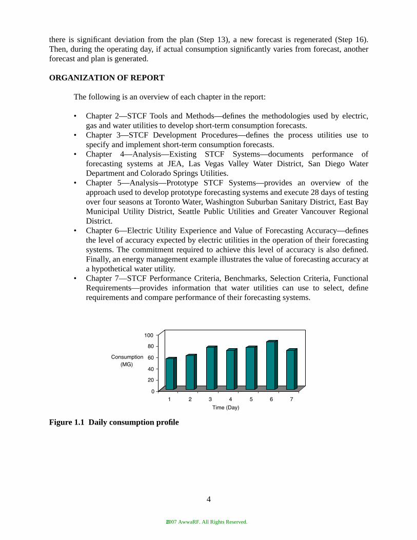
ES.5 Shifting system pumping from peak to intermediate/off-peak periods...................... xxix
1.1 Daily consumption profile.......................................................................................... 4
1.2 Hourly consumption profile ....................................................................................... 5
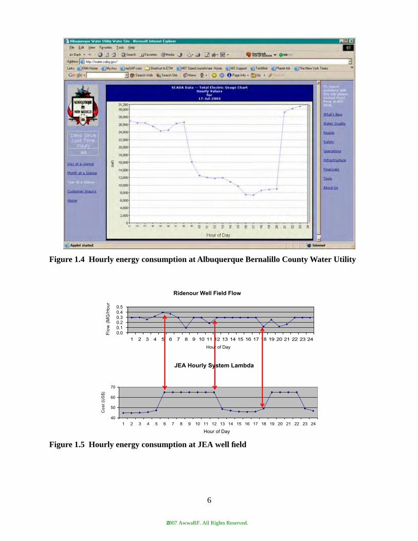
1.3 JEA operations optimization model........................................................................... 5
1.4 Hourly energy consumption at Albuquerque Bernalillo County Water Utility.......... 6
1.5 Hourly energy consumption at JEA well field ........................................................... 6
1.6 Development of system operating plan using consumption forecasting.................... 7
2.1 Daily consumption profile over a yearly period......................................................... 22
2.2 Hourly consumption profiles over a daily period....................................................... 22
2.3 Regression model example ........................................................................................ 23
2.4 Summer consumption, WWTP inflow, and rainfall ................................................... 23
2.5 Artificial neuron construction .................................................................................... 24
2.6 ANN network configuration ...................................................................................... 25
2.7 JEA Ridenour sub grid daily total forecasting results—Spring (March 2005).......... 25
3.1 Forecasting application development process............................................................ 35
3.2 Example consumption forecasting service area......................................................... 35
4.1 JEA service area......................................................................................................... 51
xi
©2007 AwwaRF. All Rights Reserved.
4.2 Example of sub grids and consumption points .......................................................... 51
4.3 JEA Ridenour sub grid hourly consumption—Summer (July 2004)......................... 52
4.4 JEA Ridenour sub grid daily consumption—Summer (July 2004) ........................... 52
4.5 JEA Ridenour sub grid hourly consumption—Fall (October 2004) .......................... 52
4.6 JEA Ridenour sub grid daily consumption—Fall (October 2004) ............................ 53
4.7 JEA Ridenour sub grid hourly consumption—Winter (January 2005)...................... 53
4.8 JEA Ridenour sub grid daily consumption—Winter (January 2005) ........................ 54
4.9 JEA Ridenour sub grid hourly consumption—Spring (March 2005)........................ 54
4.10 JEA Ridenour sub grid daily consumption—Spring (March 2005) .......................... 55
4.11 JEA Ridenour sub grid hourly consumption—Hurricane Jeanne (September 2004)....................................................................................................... 55
4.12 JEA Ridenour sub grid daily consumption—Hurricane Jeanne (September 2004)....................................................................................................... 56
4.13 LVVWD service area ................................................................................................. 56
4.14 SDWD service area.................................................................................................... 57
4.15 San Diego–Alvarado area hourly consumption—Fall (October 2004)...................... 57
4.16 San Diego–Alvarado area daily consumption—Fall (October 2004) ........................ 58
4.17 San Diego–Alvarado area hourly consumption—Winter (January 2005) ................. 58
4.18 San Diego–Alvarado area daily consumption—Winter (January 2005).................... 58
4.19 San Diego–Alvarado area hourly consumption—Spring (April 2005) ..................... 59
4.20 San Diego–Alvarado area daily consumption—Spring (April 2005) ........................ 59
4.21 San Diego–Alvarado area hourly consumption—Summer (July 2005) .................... 59
4.22 San Diego–Alvarado area daily consumption—Summer (July 2005)....................... 60
4.23 San Diego–Alvarado area hourly consumption—heavy rain (February 2005) ........ 60
xii
©2007 AwwaRF. All Rights Reserved.
4.24 San Diego–Alvarado area daily consumption—heavy rain (February 2005)........... 60
4.25 CSU service area........................................................................................................ 61
4.26 CSU system hourly consumption—Fall (October 2005)........................................... 62
4.27 CSU system daily consumption—Fall (October 2005) ............................................. 62
4.28 CSU system hourly consumption—Winter (January 2005) ...................................... 62
4.29 CSU system daily consumption—Winter (January 2005)......................................... 63
4.30 CSU system hourly consumption—Spring (April 2005)........................................... 63
4.31 CSU system daily consumption—Spring (April 2005) ............................................. 63
4.32 CSU system hourly consumption—Summer (July 2005).......................................... 64
4.33 CSU system daily consumption—Summer (July 2005) ............................................ 64
5.1 SPU service area ........................................................................................................ 78
5.2 SPU system daily consumption—Fall (October 2005).............................................. 79
5.3 SPU system daily consumption—Winter (March 2006) ........................................... 79
5.4 SPU system daily consumption—Spring (May 2006)............................................... 79
5.5 SPU system daily consumption—Summer (August 2006)........................................ 80
5.6 GVRD service area .................................................................................................... 80
5.7 GVRD system hourly consumption—Fall (November 2005) ................................... 80
5.8 GVRD test day (Fall 2005) ........................................................................................ 81
5.9 GVRD system hourly consumption—Winter (February 2006)................................. 81
5.10 GVRD test day—Winter (February 2006)................................................................. 81
5.11 GVRD system hourly consumption—Spring (May 2006) ........................................ 82
5.12 GVRD test day—Spring (May 2006) ........................................................................ 82
5.13 GVRD system hourly consumption—Summer (August 2006) ................................. 82
xiii
©2007 AwwaRF. All Rights Reserved.
5.14 GVRD test day—Summer (August 2006) ................................................................. 83
5.15 GVRD system daily consumption—Fall (November 2005)...................................... 83
5.16 GVRD system daily consumption—Winter (February 2006) ................................... 83
5.17 GVRD system daily consumption—Spring (May 2006)........................................... 84
5.18 GVRD system daily consumption—Summer (August 2006).................................... 84
5.19 EBMUD service area ................................................................................................. 85
5.20 EBMUD system hourly consumption—Fall (November 2005) ................................ 85
5.21 EBMUD test day—Fall (November 2005) ................................................................ 86
5.22 EBMUD system hourly consumption—Winter (February 2006).............................. 86
5.23 EBMUD test day—Winter (February 2006).............................................................. 86
5.24 EBMUD system hourly consumption—Spring (May 2006) ..................................... 87
5.25 EBMUD test day—Spring (May 2006) ..................................................................... 87
5.26 EBMUD system hourly consumption—Summer (August 2006) .............................. 87
5.27 EBMUD test day—Summer (August 2006) .............................................................. 88
5.28 EBMUD system daily consumption—Fall (November 2005)................................... 88
5.29 EBMUD system daily consumption—Winter (February 2006) ................................ 88
5.30 EBMUD system daily consumption—Spring (May 2006)........................................ 89
5.31 EBMUD system daily consumption—Summer (August 2006)................................. 89
5.32 Toronto water service area (including region of York) .............................................. 90
5.33 Toronto system hourly consumption—Fall (October 2005) ...................................... 90
5.34 Toronto test day—Fall (October 2005)...................................................................... 91
5.35 Toronto system hourly consumption—Winter (January 2006).................................. 91
5.36 Toronto test day—Winter (January 2006).................................................................. 91
xiv
©2007 AwwaRF. All Rights Reserved.
5.37 Toronto system hourly consumption—Spring (April 2006) ...................................... 92
5.38 Toronto test day—Spring (April 2006)...................................................................... 92
5.39 Toronto system hourly consumption—Summer (August 2006) ................................ 92
5.40 Toronto test day—Summer (August 2006)................................................................ 93
5.41 Toronto system daily consumption—Fall (October 2005) ........................................ 93
5.42 Toronto system daily consumption—Winter (January 2006) .................................... 93
5.43 Toronto system daily consumption—Spring (April 2006) ........................................ 94
5.44 Toronto system daily consumption—Summer (August 2006) .................................. 94
5.45 WSSC service area..................................................................................................... 95
5.46 WSSC system hourly consumption—Fall (October 2005)........................................ 95
5.47 WSSC test day—Fall (October 2005)........................................................................ 96
5.48 WSSC system hourly consumption—Winter (January 2006) ................................... 96
5.49 WSSC test day—Winter (January 2006) ................................................................... 96
5.50 WSSC system hourly consumption—Spring (April 2006)........................................ 97
5.51 WSSC test day—Spring (April 2006)........................................................................ 97
5.52 WSSC system hourly consumption—Summer (July 2006)....................................... 97
5.53 WSSC test day—Summer (July 2006) ...................................................................... 98
5.54 WSSC system daily consumption—Fall (October 2005) .......................................... 98
5.55 WSSC system daily consumption—Winter (January 2006)...................................... 98
5.56 WSSC system daily consumption—Spring (April 2006) .......................................... 99
5.57 WSSC system daily consumption—Summer (July 2006) ......................................... 99
5.58 Hourly AARE for all utilities..................................................................................... 99
xv
©2007 AwwaRF. All Rights Reserved.

©2007 AwwaRF. All Rights Reserved.

FOREWORD
The Awwa Research Foundation (AwwaRF) is a nonprofit corporation that is dedicated tothe implementation of a research effort to help utilities respond to regulatory requirements andtraditional high-priority concerns of the industry. The research agenda is developed through a pro-cess of consultation with subscribers and drinking water professionals. Under the umbrella of aStrategic Research Plan, the Research Advisory Council prioritizes the suggested projects basedupon current and future needs, applicability, and past work; the recommendations are forwardedto the Board of Trustees for final selection. The foundation also sponsors research projectsthrough an unsolicited proposal process; the Collaborative Research, Research Applications, andTailored Collaboration programs; and various joint research efforts with organizations such as theU.S. Environmental Protection Agency, the U.S. Bureau of Reclamation, and the Association ofCalifornia Water Agencies.
This publication is a result of one of these sponsored studies, and it is hoped that its find-ings will be applied in communities throughout the world. The following report serves not only asa means of communicating the results of the water industry’s centralized research program butalso as a tool to enlist the further support of the nonmember utilities and individuals.
Projects are managed closely from their inception to the final report by the foundation’sstaff and large cadre of volunteers who willingly contribute their time and expertise. The founda-tion serves a planning and management function and awards contracts to other institutions such aswater utilities, universities, and engineering firms. The funding for this research effort comesprimarily from the Subscription Program, through which water utilities subscribe to the researchprogram and make an annual payment proportionate to the volume of water they deliver andconsultants and manufacturers subscribe based on their annual billings. The program offers a cost-effective and fair method for funding research in the public interest.
A broad spectrum of water supply issues is addressed by the foundation’s research agenda:resources, treatment and operations, distribution and storage, water quality and analysis, toxicol-ogy, economics, and management. The ultimate purpose of the coordinated effort is to assist watersuppliers to provide the highest possible quality of water economically and reliably. The true ben-efits are realized when the results are implemented at the utility level. The foundation’s trusteesare pleased to offer this publication as a contribution toward that end.
This project was jointly funded by AwwaRF and the California Energy Commission(Energy Commission). The Energy Commission is the state’s primary energy policy and planningagency.
David E. Rager Robert C. Renner, P.E.Chair, Board of Trustees Executive DirectorAwwa Research Foundation Awwa Research Foundation
xvii
©2007 AwwaRF. All Rights Reserved.

©2007 AwwaRF. All Rights Reserved.

ACKNOWLEDGMENTS
The authors of this report are indebted to the sponsoring utilities and their staff memberswho provided project support, guidance, and data to analyze existing forecasting systems orimplement prototype applications. The sponsoring utilities and project team members follow:
JEAScott KellyDarren Hollifield
East Bay Municipal Utility DistrictDave BeyerDamon Hom
Washington Suburban Sanitary CommissionRobert TaylorTodd Supple
Greater Vancouver Regional DistrictPaul ArchibaldSharon PetersDan DonnellyTameeza JivrajJohn Pope
Las Vegas Valley Water DistrictSteven Hansen
San Diego Water DepartmentWalter Cooke
Colorado Springs UtilitiesKelvin Stone
Seattle Public UtilitiesGeorge SchneiderDan BasketfieldNian She
Toronto WaterAbhay TadwalkerCarlo CasaleRose Hosseinzadeh
The authors also acknowledge the advice and support from the Project Advisory Committee
(PAC):South Central Connecticut Regional Water AuthorityStephen Rupar
Las Vegas Valley Water AuthorityKevin Fisher
AquacraftPeter Mayer
Jennifer Warner, AwwaRF, and Paul Roggensack from the California Energy Commissionprovided project management support of this project.
Gensym Corporation provided the complimentary use of their Artificial Neural Networksoftware (NeurOn-Line) for this project.
xix
©2007 AwwaRF. All Rights Reserved.

©2007 AwwaRF. All Rights Reserved.

EXECUTIVE SUMMARY
Pumping operations at water utilities are typically consumption-following. That is, wellsand booster pumps are automatically controlled based on reservoir levels and distribution pres-sures relative to programmed setpoints. As consumption increases, levels and pressures fall andpumps are turned on. As consumption decreases, reservoir levels rise, distribution pressuresincrease, and wells and booster pumps turn off. The pumps follow consumption during the day tomaintain reservoir levels and system pressures within normal operating ranges.
While this reactive mode of operation meets operating criteria from a reliability perspec-tive, it does not leverage the opportunity to reduce operating costs as do proactive system opera-tions. Progressing to proactive system operations requires methods by which it is possible toaccurately forecast consumption on a daily (Figure ES.1) and/or hourly (Figure ES.2) basis andthen schedule water supplies, treatment, and pumping to minimize cost and maximize quality.
The objective of this research was to identify, test, and evaluate methods and tools avail-able to make short-term water consumption forecasts as required for optimizing pump schedulesand energy use and support the implementation of an Energy and Water Quality Management Sys-tem (EWQMS).
The focus of this project is on Short-Term Consumption Forecasting (STCF) as it relatesto energy, water quality, and water supply management in an operations environment. The bestrepresentation of integration of the STCF into water system operations is the EWQMS model(Figure ES.3). As shown in Figure ES.3, the Operations Planner and Scheduler (OPS), which is afunction consisting of people and software programs (system simulator and optimizer), develops aSystem Operating Plan based on the Water Consumption Forecast, Maintenance ConstructionSchedule, Energy Cost Schedule, Water Quality, Water Supply, and “The Utility’s PerformanceCriteria.” The System Operating Plan is used by system operations to optimally control treatmentplants, pumping plants, and the distribution system. The cost savings and effectiveness of optimi-zation programs are dependent on and proportional to the accuracy of the forecast. Over or underestimating consumption will result in running plants or pumps during periods of high energy andwater supply costs. Assumptions made for water quality management may be invalidated if thereare significant errors in the forecast.
SHORT-TERM CONSUMPTION FORECASTING FOR ENERGY MANAGEMENT
The water system energy management problem is essentially a mass-balance exercise. Asillustrated in Figure ES.4, the key is to move water from source to consumption area at the lowestpossible cost to take advantage of time-based electric energy rates, demand charges, pump effi-ciencies, energy production (hydro generation) and block rate energy supply contracts. It is amulti-dimensional energy supply and demand optimization problem with the common denomina-tor of time.
Short-term consumption forecasting provides the mechanism to give water customers just-in-time water supplies at minimum energy cost, considering the constraints of reservoir fire stor-age, distribution system pressure, water quality, and supply restrictions.
By accurately forecasting consumption at 15–60 minute resolution at multiple consump-tion areas in the system, water utilities have the means to leverage multiple energy management
xxi
©2007 AwwaRF. All Rights Reserved.
opportunities that can minimize cost. Opportunity can be represented from a supply and demandside perspective from the electric utility viewpoint. These opportunities are outlined as follows.
Time-of-Use Electric Rate (Demand Side)
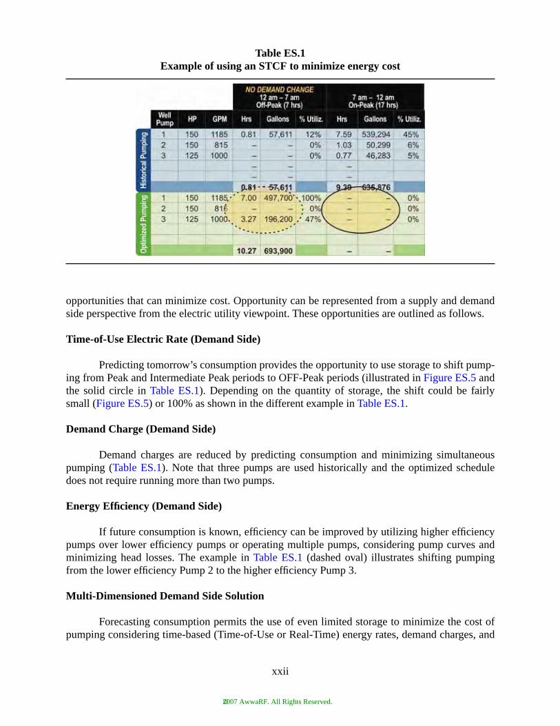
Predicting tomorrow’s consumption provides the opportunity to use storage to shift pump-ing from Peak and Intermediate Peak periods to OFF-Peak periods (illustrated in Figure ES.5 andthe solid circle in Table ES.1). Depending on the quantity of storage, the shift could be fairlysmall (Figure ES.5) or 100% as shown in the different example in Table ES.1.
Demand Charge (Demand Side)
Demand charges are reduced by predicting consumption and minimizing simultaneouspumping (Table ES.1). Note that three pumps are used historically and the optimized scheduledoes not require running more than two pumps.
Energy Efficiency (Demand Side)
If future consumption is known, efficiency can be improved by utilizing higher efficiencypumps over lower efficiency pumps or operating multiple pumps, considering pump curves andminimizing head losses. The example in Table ES.1 (dashed oval) illustrates shifting pumpingfrom the lower efficiency Pump 2 to the higher efficiency Pump 3.
Multi-Dimensioned Demand Side Solution
Forecasting consumption permits the use of even limited storage to minimize the cost ofpumping considering time-based (Time-of-Use or Real-Time) energy rates, demand charges, and
Table ES.1Example of using an STCF to minimize energy cost
xxii
©2007 AwwaRF. All Rights Reserved.

efficiency separately or simultaneously. The optimizer that minimized energy and demand cost ofwell field production shown in Table ES.1 produced a slightly higher volume of water during the24-hour period (Historical Production = 693,487 gallons, Optimized Production = 693,900 gal-lons). Pumping was rescheduled during the day to improve efficiency, minimize demand charges,and shift production to periods of the day with lower energy costs. Water consumption for the daywas satisfied with the revised schedule and tank levels were maintained within an acceptableoperating range.
Energy Resale (Supply Side)
Many public and private entities own both electric and water utilities. Combined water andelectric utilities, water utilities with hydro generation, and water utilities that purchase power inblocks, can leverage the value of energy during high cost periods if water consumption can beaccurately forecasted. During periods of the day when the value of energy is higher, pumping isreduced so energy can be sold on the spot market. When the value of energy drops during thenight, pumps are run.
Interruption (Supply and Demand Side)
Many electric utilities offer industrial customers, such as water utilities, the opportunity tosubstantially reduce energy costs with interruptible rates. If water utilities can accurately forecastconsumption, they can evaluate the impact of reduced pumping during the interruption period andbuy-through (pay a penalty) or accept the interruption period through rescheduling operations.
The decision to forecast consumption on a daily or hourly basis is significant and dependson business needs of the utility. For example, if the STCF is used for water supply and treatmentonly, then a daily forecast may be the only requirement. However, if the utility is to minimizetime-based energy cost or demand charges, then an hourly forecast is required.
Another key requirement for the STCF is the number of service areas required for fore-casting. In some cases, only a system forecast is required to satisfy optimization requirements. Inother applications it is important, from a mass-balance perspective and water conveyance perspec-tive, to forecast consumption for multiple service areas in the water system. The number of fore-casted service areas depends on the size of the utility. Large utilities may have as many as 40 or 50services areas for which forecasts are required.
METHODS AND TOOLS
Research conducted for this project identified several STCF techniques used by water, gasand electric utilities. The most common are:
• Heuristic• Linear Regression• Similar Day• Artificial Neural Network• Hybrid
xxiii
©2007 AwwaRF. All Rights Reserved.

The classic and most utilized forecasting approach by water utilities today is Heuristic, inwhich a system operator or treatment plant operator estimates today’s or tomorrow’s consumptionbased on recent consumption trends, predicted weather report, day of the week, knowledge offuture events (e.g., athletic, political, cultural), and historical knowledge of utility system perfor-mance.
Linear Regression estimates consumption based on recent consumption trends, day of theweek, weather, nonconforming and random consumption components.
The Similar Day technique searches a historical database for days in the past that hadconditions matching the projected conditions for the upcoming day. The consumption patterns foreach of these similar days are used to generate an average consumption forecast for upcomingdays.
Artificial Neural Networks (ANN) are mathematical models inspired by our understand-ing of biological nervous systems. They accept a large number of inputs which affect consump-tion and learn, from training samples, the relationships to output consumption.
Forecasting systems often use a Hybrid approach to consumption forecasting—that is, ablending of two or more methodologies. For example, a utility may choose to blend similar dayand linear regression, or ANN with statistical techniques. Again, there is one common threadthrough all the approaches—the heuristics of the human forecaster. Knowledge of the utility sys-tem, consumption patterns, and influences of other factors is required to develop a consistentlyaccurate forecast.
RESEARCH APPROACH
The approach used in the project consisted of the following phases:
• Phase 1 Initiation Researched existing STCF tools used in water, gas andelectric industries
• Phase 2 Analysis Analyzed and benchmarked STCF systems in operation atseveral utilities; developed and analyzed STCF prototypesat utilities that are not currently forecasting consumption
• Phase 3 Documentation Documented performance of the STCF systems, definedbenchmarks and develop product selection criteria
It was important that participating utilities represented multiple climatic zones (e.g.,desert, tropical, oceanic, rain forest, alpine) with multiple customer demographics. Four of theutilities had STCFs in operation or experience using STCFs.
Utility STCF Technique
Colorado Springs Utilities Similar Day
JEA ANN
San Diego ANN
Las Vegas Valley Water District Regression, ANN, Heuristic
xxiv
©2007 AwwaRF. All Rights Reserved.
Prototype STCFs were developed and tested at utilities that did not have operationalSTCFs:
RESULTS
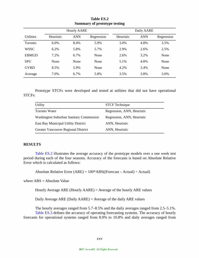
Table ES.2 illustrates the average accuracy of the prototype models over a one week testperiod during each of the four seasons. Accuracy of the forecasts is based on Absolute RelativeError which is calculated as follows:
Absolute Relative Error (ARE) = 100*ABS((Forecast – Actual) ÷ Actual)
where ABS = Absolute Value
Hourly Average ARE (Hourly AARE) = Average of the hourly ARE values
Daily Average ARE (Daily AARE) = Average of the daily ARE values
The hourly averages ranged from 5.7–8.5% and the daily averages ranged from 2.5–5.1%.Table ES.3 defines the accuracy of operating forecasting systems. The accuracy of hourly
forecasts for operational systems ranged from 8.0% to 10.8% and daily averages ranged from
Table ES.2Summary of prototype testing
Utilities
Hourly AARE Daily AARE
Heuristic ANN Regression Heuristic ANN Regression
Toronto 6.0% 8.4% 5.9% 3.0% 4.8% 3.5%
WSSC 6.2% 5.8% 5.7% 2.9% 2.6% 2.5%
EBMUD 7.2% 6.7% None 2.6% 3.2% None
SPU None None None 5.1% 4.8% None
GVRD 8.5% 5.9% None 4.2% 3.4% None
Average 7.0% 6.7% 5.8% 3.5% 3.8% 3.0%
Utility STCF Technique
Toronto Water Regression, ANN, Heuristic
Washington Suburban Sanitary Commission Regression, ANN, Heuristic
East Bay Municipal Utility District ANN, Heuristic
Greater Vancouver Regional District ANN, Heuristic
xxv
©2007 AwwaRF. All Rights Reserved.

3.2% to 4.7%. The accuracy data for operational systems was derived from weekly sample peri-ods for each season of a year.
A utility’s selection of a forecasting technique and its expected accuracy depend on theapplication(s) that are to use the forecast; initial cost and maintenance of the forecasting soft-ware/method; and complexity of the forecast (daily, hourly, system, multi-area).
Improvement in the benchmark accuracies defined in this research depends on a number offactors:
• Accuracy and repeatability of SCADA data used in the forecasts• Sophistication and calibration of the software tools• Continuous maintenance of the software tools
The accuracy of the forecasts at JEA, CSU, LVVWD and San Diego reflect real worldconditions. This includes short-term loss of SCADA data, adverse weather conditions and otheradverse/abnormal conditions. The prototypes were tested in an environment with reasonable con-trol over the operational conditions. The prototype ANN models were developed in less than aweek for each utility and the regression models were developed in a couple of days for each util-ity. The development costs were low.
Electric utilities expect average absolute percentage errors of 2.5–3.0% for hourly fore-casts in operating environments. The up front cost of achieving forecasting accuracies consistentwith this level of accuracy is high. It necessitates the purchase of an acceptable software packagethat is typically based on advanced statistical methods or Neural Network techniques. Develop-ment time for the forecaster is 12 to 14 person-months. The ongoing level of required support andmaintenance are also significant. One to two full time staff with substantial knowledge of analyti-cal forecasting techniques and system operational expertise is required. The forecasting modelrequires frequent calibration to reflect new data and system conditions. Furthermore, the forecast-ing model must be executed several times a day to reflect the changing weather conditions.
The value of an accurate short-term load forecast is very high for electric utilities. If theforecasts are inaccurate, utilities and Independent System Operators (ISOs) are forced to commitexpensive generating units at the last minute and purchase imported power at high prices. Further-more, in deregulated energy markets, load forecasts drive the clearing of the energy markets.
Table ES.3Summary of operational systems
Utilities Hourly AARE Daily AARE
JEA (ANN) 10.8% 3.9%
CSU (Similar day) 8.0% 4.1%
LVVWD* None 3.2%
San Diego (ANN) 8.0% 4.7%
Average 8.9% 4.0%
*Multiple Models—Regression, ANN, Heuristic
xxvi
©2007 AwwaRF. All Rights Reserved.
Errors in load forecast have a direct impact on the resulting locational prices and the dispatch lev-els of generating resources. In addition to the economic burden imposed on systems with poorload forecasts, forecast accuracy also directly affects the reliability of the electric network. Thestakes for accurate forecasts are obviously very high for electric utilities.
OBSERVATIONS AND LESSONS LEARNED
The following are observations and lessons learned in the execution of this 18 monthresearch project. Observations include:
• All tested methods worked well to forecast daily consumption• Daily forecasts improved when hourly data is also forecasted• ANN models appear to have better accuracy on an hour-by-hour basis than other
methods• All methods require an initial investment of labor to develop the model• ANN requires the least maintenance support• All models share a degradation in performance during seasonal and daily peak periods• Regression model requires new hourly data every day with no historical data gaps• ANN handles gaps in historical data better than regression model—only requires data
from previous day• Error or noise in recent past are reflected directly in the forecasts for both ANN and
regression models• Daily consumption correlates with type of day (weekday vs. weekend)• ANN models can be highly automated with little human intervention and support for
more complex applications• If requirements for forecasting are simple (e.g., daily and system-wide only, heuristic
approach works well
Lessons learned include:
• Accuracy of STCF is highly dependent on quality of historical data• Weather factors, other than precipitation, may not be critical to accurate forecasting• ANN models hold up well over time• Retraining an ANN may degrade the model—take care• Training ANN models with a full year of data provides better results than training with
only a single season of data• Daylight Savings Time must be accounted for to ensure data accuracy• Forecast accuracy is limited by accuracy of measurement equipment• A large number of input parameters can make models less responsive and more
difficult to maintain
xxvii
©2007 AwwaRF. All Rights Reserved.
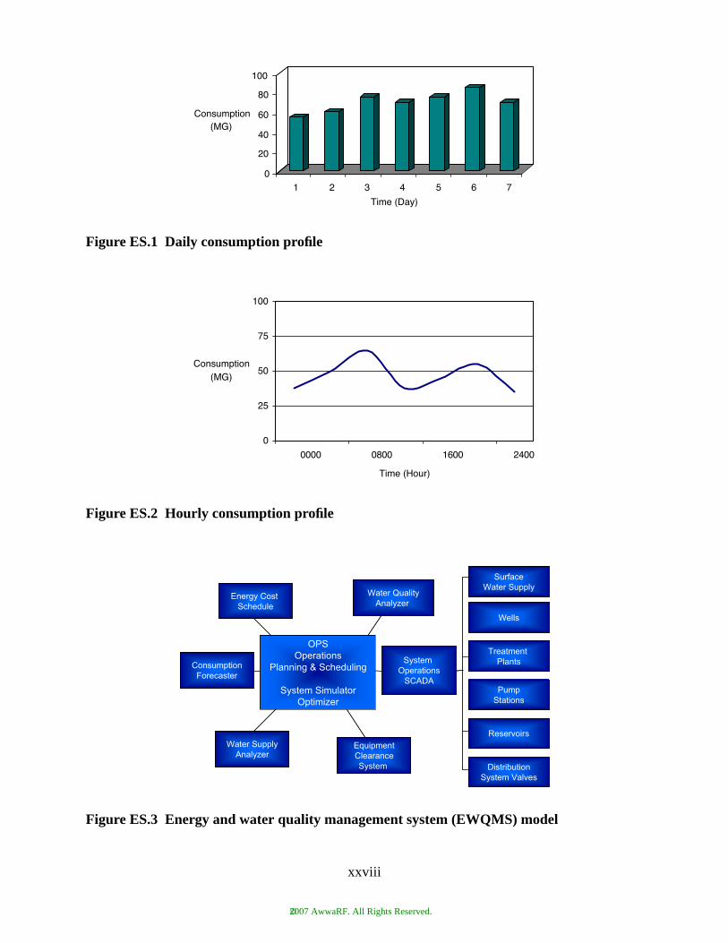
Figure ES.1 Daily consumption profile
Figure ES.2 Hourly consumption profile
Figure ES.3 Energy and water quality management system (EWQMS) model
0
20
40
60
80
100
Consumption (MG)
1 2 3 4 5 6 7
Time (Day)
0
25
50
75
100
0000 0800 1600 2400
Time (Hour)
Consumption (MG)
Wells
Treatment Plants
PumpStations
Reservoirs
DistributionSystem Valves
System Operations
SCADA
EquipmentClearanceSystem
OPSOperations
Planning & Scheduling
System SimulatorOptimizer
Water QualityAnalyzer
Energy Cost Schedule
ConsumptionForecaster
Water SupplyAnalyzer
SurfaceWater Supply
Wells
Treatment Plants
PumpStations
Reservoirs
DistributionSystem Valves
System Operations
SCADA
EquipmentClearanceSystem
OPSOperations
Planning & Scheduling
System SimulatorOptimizer
Water QualityAnalyzer
Energy Cost Schedule
ConsumptionForecaster
Water SupplyAnalyzer
SurfaceWater Supply
xxviii
©2007 AwwaRF. All Rights Reserved.
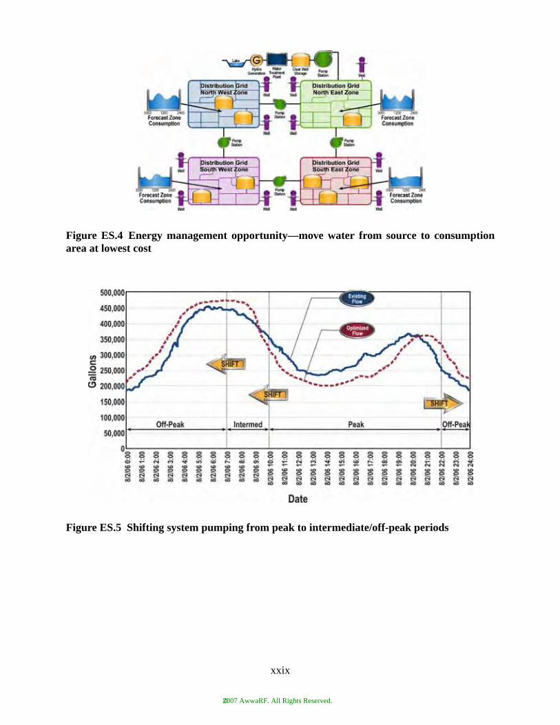
Figure ES.4 Energy management opportunity—move water from source to consumptionarea at lowest cost
Figure ES.5 Shifting system pumping from peak to intermediate/off-peak periods
xxix
©2007 AwwaRF. All Rights Reserved.

©2007 AwwaRF. All Rights Reserved.

CHAPTER 1BACKGROUND AND INTRODUCTION
BACKGROUND
Water utilities have traditionally used computer based tools for forecasting consumption; prima-rily for long term master planning. Water systems were planned, designed, and constructed tomeet the future needs of the community. However, experience of the industry in short-term fore-casting for optimizing operations is limited.
Pumping operations at water utilities are typically consumption-following. That is, wellsand booster pumps are automatically controlled based on changes in reservoir levels and distribu-tion pressures. As consumption increases, levels and pressures fall and pumps are turned on. Asconsumption decreases, reservoir levels rise, distribution pressures increase, and wells andbooster pumps turn off. The pumps “follow” consumption during the day to keep reservoir levelsand system pressures within normal operating ranges.
While this reactive mode of operation meets operating criteria from a reliability perspec-tive, it fails to leverage the opportunity to reduce operating cost and maximize water quality andsupply associated with proactive system operations.
The objective of this research was to identify, test and evaluate available methods andtools for making short-term water consumption forecasts. These short-term forecasts are requiredfor optimizing pumping schedules and energy use and to support the implementation of an Energyand Water Quality Management System (EWQMS).
Long-Term Consumption Forecasting
A Long-Term Consumption Forecast (LTCF) typically covers a period of 10 to 20 years.Key factors in developing the forecast include industrial, commercial and residential growth;rates; conservation; and weather conditions. The LTCF is then used by system planners and engi-neers to finance, design and construct new water facilities. The LTCF is a key component of thehydraulic model used to simulate and analyze expansion of new facilities and pipelines. Thesystem planner is typically interested in peak and average day analysis of the system. The modelsare often integrated with Geographic Information Systems (GIS) and represent thousands of pipesections and nodes.
Short-Term Consumption Forecasting
The planning horizon for a Short-Term Consumption Forecast (STCF) is significantlyshorter than the LTCF. The STCF is used for day-to-day water system operations planning with atypical horizon from one hour to one week. The operations planner requires a forecastedconsumption profile with daily (Figure 1.1) and, hourly (Figure 1.2) resolution to schedule rawwater delivery, treatment plant production and distribution system pumping. The STCF isprepared on a system and operating area basis (e.g., area, zone, subgrid, tank). The objective is tominimize the cost of operation to meet consumption considering the constraints of reservoir
1
©2007 AwwaRF. All Rights Reserved.

levels, pressures, and system configuration. Significant savings in energy, water supply, and treat-ment costs can be achieved through optimized scheduling of the system assets based on the STCF.Application of an STCF can move a water utility from a reactive to a proactive mode of operation.
APPLICATIONS FOR SHORT-TERM CONSUMPTION FORECASTING
An STCF enables many operational applications for a water utility—energy, water quality,water supply and maintenance management. An example of the integration of an STCF into opti-mization of operations at JEA (Jacksonville, Florida) is shown in Figure 1.3.
JEA forecasts consumption for multiple areas or subgrids as the key driver to their Opera-tions Optimization System. Daily and weekly forecasts are used by the OperationsPlanner/Scheduler to schedule well field production and high service pumping. An annual fore-cast is used by the Water Supply Analyzer to schedule water plants to meet the consumptive usepermit of the Floridan aquifer.
Energy Management
Forecasting daily consumption with one hour resolution is a key factor for water utilitieswho deal with Time-of-Use (TOU) or real-time pricing schedules from their energy suppliers.Forecasting hourly consumption at an operating area, zone or reservoir provides the means toproduce and transfer water during off-peak hours or low cost periods. The strategy is to usestorage to minimize pumping during the on-peak or higher cost periods of the day. An effectiveforecast provides the means for “Just-in-Time” production and supply of water to customers byusing reservoir storage capacity efficiently.
Figure 1.4 illustrates how effectively Albuquerque produces water from wells and trans-fers the water to reservoirs during off-peak hours. Figure 1.4 is a trend of aggregate water systemenergy consumption for 24 hours. The graph illustrates the low level of pumping during on-peakhours (8:00 AM–8:00 PM) and the high level of pumping during off-peak hours (8:00 PM–8:00 AM). Consumption is calculated and heuristically forecasted for each reservoir in the system.The savings in energy costs is over a million dollars a year.
Some water utilities have flat or constant energy rates with a demand charge. The demandcharge is based on the peak power consumed at a facility over a set period of time-typically onemonth. In this case, simultaneous pumping from multiple pumps can be reduced to minimize thedemand change and meet forecasted consumption. The strategy is to run pumps consecutively forlonger periods with as few pumps run concurrently as necessary to meet forecasted consumption.
Other utilities have real-time pricing for electrical or gas energy. In this case, the cost ofenergy varies by the hour during the day. Again, if water consumption is accurately forecasted, thewater utility can minimize cost by pumping during low cost periods.
Figure 1.5 illustrates well field pumping at JEA in response to a real-time cost structure.In a similar manner to reducing demand charges, energy efficiency can be improved
through selection of pumping combinations that take into account pump discharge head curves.By considering the consumption forecast, a pump schedule can be generated that maximizesstation efficiency and maintains distribution pressures and reservoir levels within acceptable oper-ating ranges.
Finally, hourly and daily consumption forecasts are useful for scheduling hydro generationunits to maximize the value of energy production from these units. Power produced during
2
©2007 AwwaRF. All Rights Reserved.

on-peak hours has more value than power produced off-peak. The strategy is to move water withinthe water distribution system in such a way that storage is available for hydro generation duringon-peak hours.
Water Supply
Daily, hourly, and annual consumption forecasts are used to schedule raw water suppliesand production from water treatment plants. Many water utilities have multiple sources of supplyand optimally scheduling these supplies to minimize operating cost can yield significant results.San Diego Water Department had substantial savings in water supply costs through the use of aconsumption forecaster and water supply optimizer. The savings in the first year of operation ofthe Water Supply Optimizer was approximately $800,000. This is in addition to over $300,000savings in annual energy costs.
Water Quality
Water quality can be enhanced by proactive operation of the water system with aconsumption forecaster. Drafting reservoirs on a regular basis to minimize water age is oneexample. In this case, pumps are scheduled to draft and then fill reservoirs based on daily andweekly forecasted consumption.
Scheduling Maintenance and Construction
Proactive scheduling of maintenance and construction to minimize cost, maintain highsystem reliability, and optimize system water quality is facilitated by consumption forecasting. Anhourly and daily schedule for system operations to minimize disruption from maintenance andconstruction can be developed based on forecasted consumption.
Proactive System Operations
These examples illustrate the opportunities for proactive operations. Consumption fore-casting provides the means for the Operations Planner to substantially reduce operating costs anddeliver a high quality product to customers. One or several of these examples may provide a basisfor development of a valid business case to move the utility to implement short-term consumptionforecasting.
Integration of Consumption Forecasting Into Operations Management
A consumption forecast is typically prepared on an annual, weekly, and daily basis to opti-mally plan and schedule system operations. Figure 1.3 illustrates the model for integration ofconsumption forecasting for energy, water supply and water quality management at JEA.
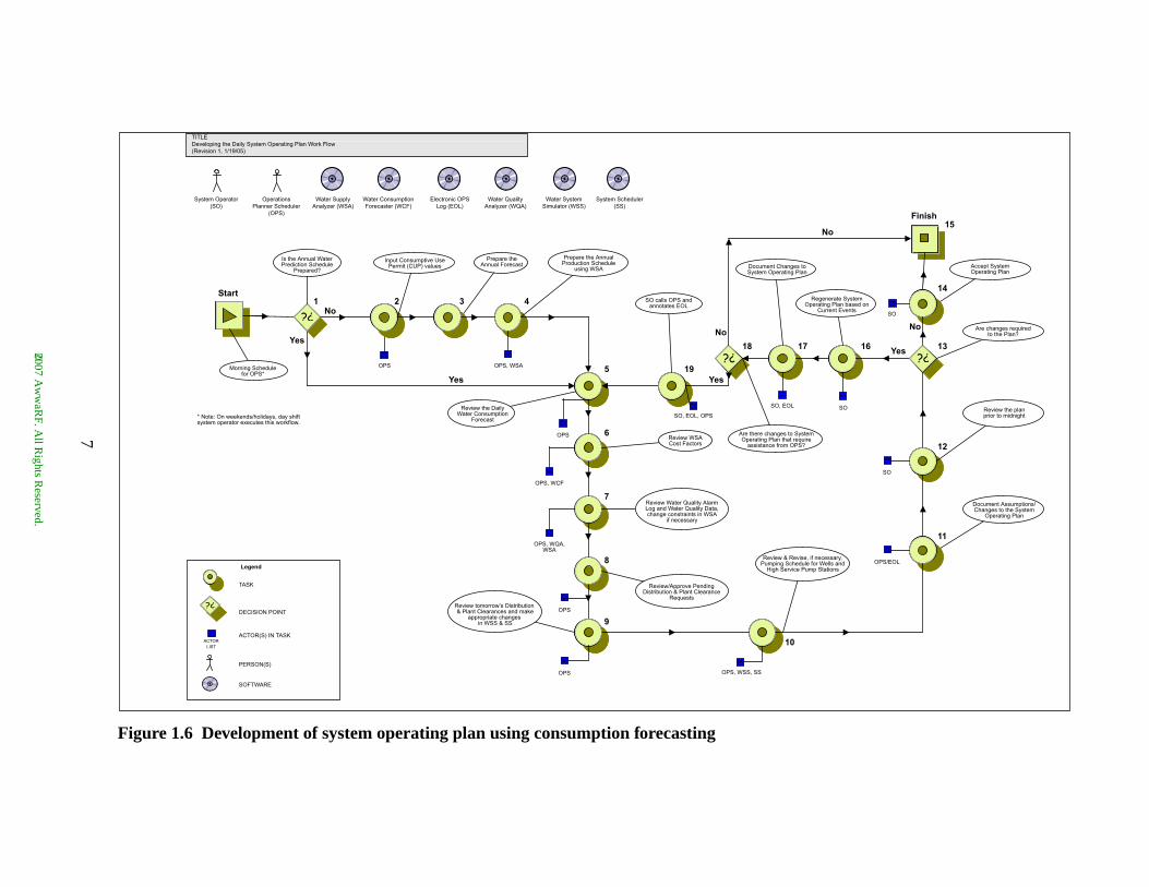
Figure 1.6 illustrates a conceptual workflow for development of a daily system operatingplan based on consumption forecasting. Note that an Annual Consumption Forecaster (Step 3) isused to develop the water production schedule for the year. The Daily Water Consumption Fore-cast (Step 5) is used to schedule maintenance (Clearance Requests), water production andpumping. Prior to accepting the Operating Plan at midnight, operation conditions are reviewed. If
3
©2007 AwwaRF. All Rights Reserved.
there is significant deviation from the plan (Step 13), a new forecast is regenerated (Step 16).Then, during the operating day, if actual consumption significantly varies from forecast, anotherforecast and plan is generated.
ORGANIZATION OF REPORT
The following is an overview of each chapter in the report:
• Chapter 2—STCF Tools and Methods—defines the methodologies used by electric,gas and water utilities to develop short-term consumption forecasts.
• Chapter 3—STCF Development Procedures—defines the process utilities use tospecify and implement short-term consumption forecasts.
• Chapter 4—Analysis—Existing STCF Systems—documents performance offorecasting systems at JEA, Las Vegas Valley Water District, San Diego WaterDepartment and Colorado Springs Utilities.
• Chapter 5—Analysis—Prototype STCF Systems—provides an overview of theapproach used to develop prototype forecasting systems and execute 28 days of testingover four seasons at Toronto Water, Washington Suburban Sanitary District, East BayMunicipal Utility District, Seattle Public Utilities and Greater Vancouver RegionalDistrict.
• Chapter 6—Electric Utility Experience and Value of Forecasting Accuracy—definesthe level of accuracy expected by electric utilities in the operation of their forecastingsystems. The commitment required to achieve this level of accuracy is also defined.Finally, an energy management example illustrates the value of forecasting accuracy ata hypothetical water utility.
• Chapter 7—STCF Performance Criteria, Benchmarks, Selection Criteria, FunctionalRequirements—provides information that water utilities can use to select, definerequirements and compare performance of their forecasting systems.
Figure 1.1 Daily consumption profile
0
20
40
60
80
100
Consumption (MG)
1 2 3 4 5 6 7
Time (Day)
4
©2007 AwwaRF. All Rights Reserved.
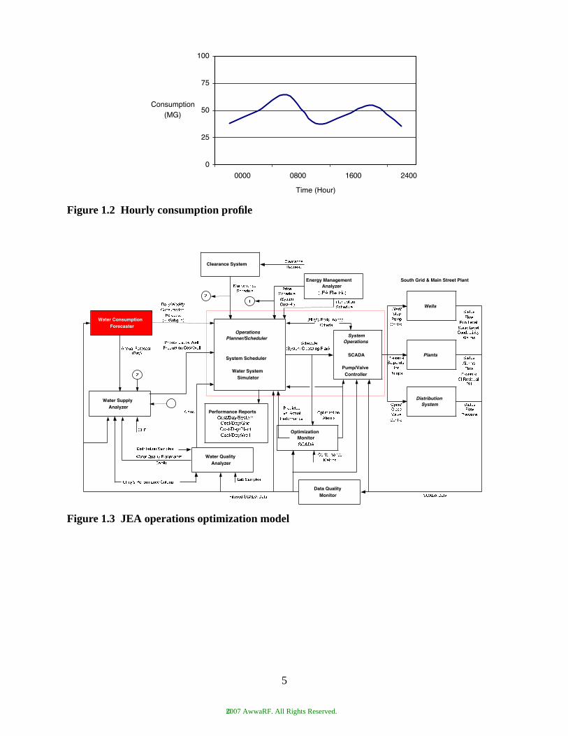
Figure 1.2 Hourly consumption profile
Figure 1.3 JEA operations optimization model
0
25
50
75
100
0000 0800 1600 2400
Time (Hour)
Consumption (MG)
Water Consumption Forecaster
Performance Reports����������������������� ��
��������������
������������
Distribution System
�������������� ����������
South Grid & Main Street Plant
�� ���������������� ��
� ��� ���������
�� ������
������������������ ��
���������
����������������������������
��� ��
�������� ��
����
� ��� ���������
�
���������
� ���
���� ����
��� ���������
��������������
���������� �� ������ �� ��
� �� �����������
���������
�
� �
��������� ���������
����������������������
�� ������ ���� ��
� �� ���������������
� ������������������
���������� �� ������ �� ��
��� ����������� ��� ������
���� �������������
� �����������������
� �� ������ ��
����� ������� ���
�
���� � ���� ����
Clearance System
Energy Management Analyzer
��������� ��
�
���������������� ��
Plants
Wells
� ��������������������
Water Supply Analyzer
Operations Planner/Scheduler
System Scheduler
Water System Simulator
Water Quality Analyzer
Optimization Monitor����
Data Quality Monitor
System Operations
SCADA
Pump/Valve Controller
5
©2007 AwwaRF. All Rights Reserved.
6
Figure 1.4 Hourly energy consumption at Albuquerque Bernalillo County Water Utility
Figure 1.5 Hourly energy consumption at JEA well field
0.00.10.20.30.40.5
1 2 3 4 5 6 7 8 9 10 11 12 13 14 15 16 17 18 19 20 21 22 23 24
Hour of Day
uo
H/G
M( w
olF
r
40
50
60
70
1 2 3 4 5 6 7 8 9 10 11 12 13 14 15 16 17 18 19 20 21 22 23 24
Hour of Day
$S
U( tso
C)
Ridenour Well Field Flow
JEA Hourly System Lambda
©2007 AwwaRF. All Rights Reserved.
7
t Changes toperating Plan
Accept SystemOperating Plan
Are changes requiredto the Plan?
Review the planprior to midnight
OPS/EOL
SO
SOSO, EOL
SO
Regenerate SystemOperating Plan based on
Current Events
Document Assumptions/Changes to the System
Operating Plan
nges to Systemlan that requiree from OPS?
iew & Revise, if necessary,ping Schedule for Wells and
igh Service Pump Stations
Finish
10
11
12
131617
14
15
Yes
No
No
©2007 Aw
waR
F. All R
ights Reserved.
Figure 1.6 Development of system operating plan using consumption forecasting
TITLEDeveloping the Daily System Operating Plan Work Flow(Revision 1, 1/19/05)
System Operator(SO)
OperationsPlanner Scheduler
(OPS)
Water SupplyAnalyzer (WSA)
Water ConsumptionForecaster (WCF)
Electronic OPSLog (EOL)
Water QualityAnalyzer (WQA)
Water SystemSimulator (WSS)
System Scheduler(SS)
Input Consumptive UsePermit (CUP) values
Prepare theAnnual Forecast
SO calls OPS andannotates EOL
DocumenSystem O
Review WSACost Factors
Morning Schedulefor OPS*
Is the Annual WaterPrediction Schedule
Prepared?
OPS
OPS
SO, EOL, OPS
OPS
OPS
OPS, WSA
OPS, WCF
OPS, WQA,WSA
OPS, WSS, SS
Prepare the AnnualProduction Schedule
using WSA
Are there chaOperating P
assistanc
Review Water Quality AlarmLog and Water Quality Data,change constraints in WSA
if necessary
Review tomorrow’s Distribution & Plant Clearances and make
appropriate changes in WSS & SS
Review/Approve PendingDistribution & Plant Clearance
Requests
Review the DailyWater Consumption
Forecast
RevPum
H
* Note: On weekends/holidays, day shiftsystem operator executes this workflow.
Legend
TASK
DECISION POINT
ACTOR(S) IN TASK
PERSON(S)
SOFTWARE
ACTORLIST
Start1 2 3 4
5 19
6
7
8
9
18Yes
Yes Yes
No
No

©2007 AwwaRF. All Rights Reserved.

CHAPTER 2STCF TOOLS AND METHODS
INTRODUCTION
This chapter identifies short-term consumption forecasting tools and methods in currentuse by electric, gas and water utilities. The research on existing tools and methods was conductedto focus the STCF prototype work on this project to methodologies which would be most likelyimplemented by water utilities. This background work should be useful to any water utilityconsidering consumption forecasting.
An STCF is an important operational tool for all utilities. Research indicates the fore-casting tools and procedures used in the various utility sectors are very similar.
WATER UTILITY FORECASTING BACKGROUND
Until recently, water utility consumption forecasting efforts were limited to long-termconsumption forecasts used for water supply and facility planning. Interest in short-termconsumption forecasting for day-to-day operations use began in the 1980s.
U.S. research into short-term consumption forecasting methods and tools includes Maid-ment et al. (1985) and Jain and Ormsbee (2002). European water utilities have also investigatedshort-term consumption forecasting, including Coulbeck et al. (1985) and Crommelynck et al.(1991 approx). In general, early research used regression and time-series modeling techniques,while more recent research has focused on Artificial Intelligence (AI) techniques including ExpertSystems and Artificial Neural Networks (ANN).
Jain and Ormsbee’s July 2002 Journal AWWA article provides a concise summary ofvarious short-term water consumption forecasting methods, and compares their performance inforecasting water consumption at Lexington, Kentucky.
ELECTRIC UTILITY FORECASTING BACKGROUND
Compared to water utilities, electric utilities have longer experience using short-termconsumption forecasting. Short-term consumption forecasting is an integral component of electricutility Energy Management Systems (EMS) which has been in wide use since the late 1970s andearly 1980s.
Like the water utility industry, the earliest short-term electrical consumption forecastingtechniques used regression models, while more recent implementations have used ExpertSystems, ANNs, “Fuzzy Logic” and various combinations of the above.
Papalexopoulos and his associates (1990 and 1994) have implemented both regression andANN forecasting models and compared their performance. Sugianto and Lu have prepared abibliography survey of the consumption forecasting techniques used in the electric utilityindustry.
9
©2007 AwwaRF. All Rights Reserved.

GAS UTILITY FORECASTING BACKGROUND
Gas utilities also routinely use short-term gas consumption forecasting in their daily oper-ations. Forecasting is important in scheduling effective use of gas pipeline transmission capacity.
As in the water and electric utility industries, the most recent short-term gas consumptionforecasting implementations have focused on ANN models. Lamb and Logue (2001) presented aninsightful summary of the design, implementation, training and testing process for an ANN-basedgas consumption forecasting application. This paper provides good background material for anyentity considering implementation of consumption forecasting. Another treatise on gas consump-tion forecasting is presented by Khotanzad (1999).
WATER CONSUMPTION PATTERNS, TERMINOLOGY, AND FORECASTING CONCEPTS
The following section describes basic water consumption patterns and forecastingconcepts in terms of:
• Daily water use variations over a yearly period• Daily water use variations over a weekly period• Hourly water use variations over a daily period
Daily consumption forecasts are required for optimal production management applica-tions. Thus, daily consumption variations over yearly and weekly time periods are evaluated.Hourly consumption forecasts are required for optimal energy and water quality managementapplications. Thus, hourly consumption variations over daily time periods are evaluated as well.
Daily Water Use Variations Over a Yearly Period
Figure 2.1 shows a representative water utility daily total consumption profile for a one-year period beginning in September, 1996. For most water utilities in the United States, dailyconsumption follows the general pattern illustrated in Figure 2.1. Water consumption is lowest inthe winter, with relatively small variations in daily consumption. In the spring, consumptionbegins to rise, peaking in mid summer, and dropping again in the fall. During high consumptionperiods, daily consumption variations can be quite large, depending on conditions and individualutility circumstances.
Many water utilities explain this general pattern by classifying water use into two parts:Base Consumption—which includes normal indoor residential and industrial water use; andIrrigation Consumption—which includes all outdoor water uses. Figure 2.1 shows the base andirrigation components of consumption.
Base Consumption
Base Consumption is primarily based on and determined by the number of water users. Itcan change over time with migration, due to permanent population growth or decline; or due toseasonal migration in and out of the service area. For combined water/wastewater utilities, wherethe water and wastewater service areas are essentially the same, wastewater treatment plant flow
10
©2007 AwwaRF. All Rights Reserved.

can provide an accurate estimate of Base Consumption if Infiltration and Inflow (I&I) effects aresmall. Also, for northern cities with minimal winter Irrigation Consumption, winter consumptiontrends provide a good estimate of base consumption.
Irrigation (Seasonal) Consumption
Given these assumptions, Irrigation Consumption generally only occurs when the airtemperature is above freezing. In the northern states, winter irrigation consumption is essentiallyzero. In southern states, irrigation occurs throughout the year.
In the scenario described above, winter Irrigation Consumption is primarily driven by airtemperature, especially in the colder states. In warmer states, where irrigation occurs all yearlong, the secondary drivers for winter Irrigation Consumption include rainfall, temperature andsolar radiation (i.e., length of the day and amount of cloud cover.)
Assuming that most summer Irrigation Consumption is used for lawn and gardenwatering, the fundamental driving force for summer Irrigation Consumption is the additionalwater required for healthy plant growth (e.g., lawn and garden plant evapotranspiration require-ments minus the amount of rainfall.) This explains the typical seasonal variation that starts low inspring, peaks in mid summer, and tapers off in the fall.
In this scenario, Summer Irrigation consumption is primarily driven by the followingfactors:
• Number of water users• Percent of the service area under irrigation• Irrigation rules or restrictions placed by the water utility• Irrigation practices of the water users (including factors associated with automatic
sprinkler system use)• Rainfall• Air temperature
Secondary drivers for summer Irrigation Consumption include other factors that affectevapotranspiration requirements including:
• Amount of solar radiation (length of day and amount of cloud cover)• Wind speed• Humidity
Daily Water Use Variations Over a Weekly Period
In many water utilities, consumption follows a periodic weekly pattern. However, theconsistency and details of the weekly pattern depend on individual utility conditions and circum-stances. When evaluating weekly consumption patterns, it is important to recognize that majorholidays usually disrupt the normal weekly cycle. Often, consumption on these days must betreated as a special case.
During spring, summer, and fall when significant irrigation consumption occurs, thehourly consumption pattern shifts to reflect irrigation practices of water users.
11
©2007 AwwaRF. All Rights Reserved.

Hourly Water Use Variations Over a Daily Period
For most utilities, hourly water consumption usually follows a fairly regular 24-hourpattern, with the pattern changing according to day of the week and season.
Figure 2.2 shows average hourly consumption for each day of the week during July 2005in Colorado Springs. The hourly consumption patterns for all days except Friday are very similarwith peak flow occurring at 06:00–07:00 and 20:00–22:00. The hourly consumption pattern forFriday appears unique. This could be an anomaly in this data, or it could represent the fact thatFriday is a transition day between the normal work week and the weekend.
During spring, summer and fall when significant Irrigation Consumption occurs, thehourly consumption patterns shift to reflect irrigation practices of water users.
In summary, hourly consumption variations over a daily time frame are generally driven by:
• Water use practices and lifestyle of the utility customers• Day of the week• Season • Irrigation practices of utility customers, including preferences for watering during the
day or at night, and automatic sprinkler system timer settings• Irrigation rules or restrictions placed by the water utility
WATER CONSUMPTION FORECASTING PROBLEM DEFINITION
The objectives of this project are to identify, test, and evaluate available methods and toolsfor making short-term water consumption forecasts, necessary for optimizing pumping schedulesand energy use, to support the implementation of an Energy and Water Quality ManagementSystem (EWQMS). Meeting this objective requires forecasting daily consumption for one ormore days into the future. It also requires forecasting hourly consumption for 24 or more hoursinto the future.
With this in mind, the formal definition of the forecasting problem addressed by thisproject is to:
• For a well-defined service area, forecast daily total water consumption for one to sevendays into the future
• For a well-defined service area, forecast hourly average water consumption for 24 to48 hours into the future
INTRODUCTION TO FORECASTING METHODS
This section presents a brief overview of the most common short-term consumption fore-casting techniques used in the water, electric and gas utility industries. This overview is notrigorous, and focuses on concepts over mathematical and statistical theory. Readers who desire amore in-depth discussion of the various forecasting techniques should consult the references listedat the end of this report.
Short-term consumption forecasting is broken into two separate problems—daily consump-tion forecasting and hourly consumption forecasting. With this in mind, common methods for fore-casting daily and hourly consumption are discussed separately in the following text.
12
©2007 AwwaRF. All Rights Reserved.

DAILY CONSUMPTION FORECASTING METHODS
The most common utility industry daily consumption forecasting techniques are:
• Regression Models• Time Series Models• Artificial Neural Network Models• Expert System (Rule-Based) Models• Similar Day Models• Heuristic Models• Various Combinations of the Above
The basic concepts behind each of these techniques are briefly summarized in this section.
Regression Model Techniques
A regression model is a standard statistical technique which relates various input variablesto an output variable using a multi-variable linear equation. Equation parameters are computed soas to minimize the overall error between predicted output and observed output values.
The following regression model form is often used in a daily consumption forecastingapplication:
Today’s Forecasted Consumption= Constant+ A * Previous Day Demand+ B * Previous Day (or Days) Rainfall+ C * Today’s Forecasted Max Temperature+ D * Today’s Forecasted Rainfall
However, for any given utility, the appropriate regression model inputs have to be selectedbased on which input variables are most highly correlated to daily consumption.
Figure 2.3 shows an example of a regression model for daily consumption. The figureshows the raw data, regression coefficients, and a plot of the actual and predicted total dailyconsumption. In this particular model, daily consumption was regressed against yesterday’sconsumption, current day rainfall, current day maximum temperature, and current day solar radia-tion using data from the past two weeks. At the beginning of any day, today’s consumption is fore-casted by inputting yesterday’s consumption and today’s forecasted rainfall, maximumtemperature, and estimate of solar radiation based on the “cloudiness” forecast.
To compensate for the fact that regression model parameters are non-linear and vary withtime, this particular model updated the regression model parameters every day using the last twoweeks of data. This approach had acceptable performance under normal circumstances, but wasadversely affected by unusual events (holidays, etc.) that disrupted the normal consumptionpattern for any given day. In the figure, one of these events occurred on June 17th, where theactual consumption was significantly less than predicted. Not only did the regression model give apoor estimate for this day, this error was also propagated into future days where the regression
13
©2007 AwwaRF. All Rights Reserved.
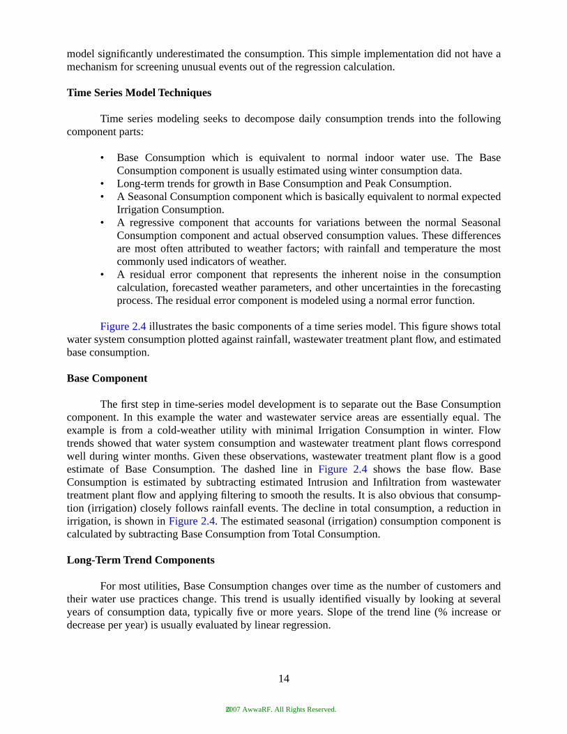
model significantly underestimated the consumption. This simple implementation did not have amechanism for screening unusual events out of the regression calculation.
Time Series Model Techniques
Time series modeling seeks to decompose daily consumption trends into the followingcomponent parts:
• Base Consumption which is equivalent to normal indoor water use. The BaseConsumption component is usually estimated using winter consumption data.
• Long-term trends for growth in Base Consumption and Peak Consumption.• A Seasonal Consumption component which is basically equivalent to normal expected
Irrigation Consumption.• A regressive component that accounts for variations between the normal Seasonal
Consumption component and actual observed consumption values. These differencesare most often attributed to weather factors; with rainfall and temperature the mostcommonly used indicators of weather.
• A residual error component that represents the inherent noise in the consumptioncalculation, forecasted weather parameters, and other uncertainties in the forecastingprocess. The residual error component is modeled using a normal error function.
Figure 2.4 illustrates the basic components of a time series model. This figure shows totalwater system consumption plotted against rainfall, wastewater treatment plant flow, and estimatedbase consumption.
Base Component
The first step in time-series model development is to separate out the Base Consumptioncomponent. In this example the water and wastewater service areas are essentially equal. Theexample is from a cold-weather utility with minimal Irrigation Consumption in winter. Flowtrends showed that water system consumption and wastewater treatment plant flows correspondwell during winter months. Given these observations, wastewater treatment plant flow is a goodestimate of Base Consumption. The dashed line in Figure 2.4 shows the base flow. BaseConsumption is estimated by subtracting estimated Intrusion and Infiltration from wastewatertreatment plant flow and applying filtering to smooth the results. It is also obvious that consump-tion (irrigation) closely follows rainfall events. The decline in total consumption, a reduction inirrigation, is shown in Figure 2.4. The estimated seasonal (irrigation) consumption component iscalculated by subtracting Base Consumption from Total Consumption.
Long-Term Trend Components
For most utilities, Base Consumption changes over time as the number of customers andtheir water use practices change. This trend is usually identified visually by looking at severalyears of consumption data, typically five or more years. Slope of the trend line (% increase ordecrease per year) is usually evaluated by linear regression.
14
©2007 AwwaRF. All Rights Reserved.

Many water utilities also show a long-term trend in peak water use over several years, andagain, this trend is usually identified by visual examination of several years of data. Changes inpeak use result from changes in the number of customers and their irrigation practices. If a peakuse trend exists, various statistical methods are used to subtract the trend from the data set prior tofurther analysis.
The next step in time series analysis is to develop a function that represents the averageoverall shape of the Irrigation Consumption component. In this example, a trigonometric expres-sion called the Sinc Function is used to represent the normal seasonal variations in IrrigationConsumption, assuming average weather conditions.
The final step is to model the difference between the expected irrigation (seasonal) compo-nent and actual observed irrigation. In time series forecasting, this is the point where developingthe appropriate model is as much an art as it is a science. In this example, temperature and rainfallare used.
This illustrative example uses a very simple technique to relate rainfall and changes inconsumption. The basic assumption is this: if it rains today, today’s total irrigation consumptionwill decrease by a given percentage. If it is dry today, today’s irrigation consumption will increasetoward the maximum expected dry-period irrigation amount (Sinc Function) by a givenpercentage of the difference between yesterday’s irrigation and the maximum expected irrigation.This technique was implemented in a forecasting application using a yes/no rain forecast based onthe forecasted chance of rain. The Total Consumption forecast for the day is the sum of Base andthe seasonal forecast components.
Time series models do not expect to be 100% accurate. As a result, they include a randomerror component that mimics the normal expected variations in actual consumption and theconsumption forecasting process. The residual error between forecasted and actual irrigation ismodeled as a normal distribution with mean of zero and standard deviation of the residual errorresults.
The Average Absolute Relative Error (AARE) measurement is used to benchmark STCFaccuracy. AARE is a standard measure of forecasting accuracy and is defined as:
Relative Error = 100*(Forecasted Value – Observed Value)/Observed ValueAARE = Sum of absolute value of relative errors divided by number of observations.
Artificial Neural Network (ANN) Model Technique
An ANN mimics the way a human brain processes data by simulating the action of biolog-ical neurons as shown in Figure 2.5. The upper half of Figure 2.5 shows a biological neuron, andthe lower half shows the computer analog used in ANN models.
The human brain is composed of a countless number of neurons linked through a web ofnervous system connectors called Axons, which transmit the nervous system’s “signal” betweenneurons. Each neuron can receive input signals from many other neurons via Axon connector sitescalled Dendrites. The input signals pass between Axon and Dendrite through a Synaptic Junction.The neuron’s cell body—called the Soma—processes the combined signal and passes it to andoutput Axon, which carries the output signal to other neurons.
A baby is born with about 100 billion neurons, with each neuron connected to about 1000other neurons. The baby’s brain learns by adjusting the “signal strength” passing through everySynaptic Junctions between Axon and Dendrite.
15
©2007 AwwaRF. All Rights Reserved.

ANN models are built by assembling a network of artificial neurons. ANN models cancontain only a few dozen or a few hundred neurons, so they are much simpler and more limited thanthe human brain. However, a simple ANN network can “learn” to do one specific task very well.
As shown in Figure 2.5, the artificial neuron has a number of inputs from other neurons.Each input signal is multiplied by a weighting factor, and the resulting weighted signals aresummed within the artificial neuron. This mimics the process that happens in biological neurons,with the input weights representing signal strength crossing a synaptic junction.
Within the artificial neuron, the weighted sum of inputs is processed through an activationfunction before sending the output to other neurons. Many different activation functions are avail-able, with the selection of activation function tailored to the specific application. In forecastingapplications, the most common activation function is the Logistic Sigmoid Function. This partic-ular sigmoid function is non-linear. Use of a non-linear activation function is what gives ANNmodels their ability to handle non-linear relationships between model inputs and outputs.
ANN models are constructed by configuring a network of artificial neurons built in layers.A simple example illustrates how an ANN works. Table 2.1 contains data collected for a process,the nature of which is not important for this discussion.
Parameters A and B are input variables, and the requirement is to predict the value of C forcombinations of A and B. The ANN model can be thought of as a process estimator where A andB are inputs and a predicted value of C is the output, as shown in Figure 2.6.
Inside the process predictor, the ANN consists of nodes that are arranged in layers asshown in Figure 2.6. The nodes (u) in each layer are connected to the nodes of the next layer tocreate a network. Each connection is assigned a weight (w) that is used to calculate values foreach node. To solve more complex problems, more layers are configured and more nodes areadded to each layer.
This ANN consists of three (3) layers. In the first layer, the nodes contain the input values(A and B) and a constant value of 1. The second layer consists of three nodes that will contain theresults of calculations resulting from the values in the nodes of layer 1 and the weighted connec-tions between layer 1 and layer 2. The third layer, in this case the output layer, contain only onenode that contains the results of calculations resulting from the values in the nodes of layer 2 and
Table 2.1ANN inputs and predicted output
Input A Input B Output C ANN Predicted C
5 5 1 0.999991
12 4 3 2.999993
15 3 5 4.999995
21 3 7 6.999999
27 3 9 9.000007
40 4 10 10.000009
40 5 8 8.000004
42 7 6 5.999999
44 11 4 4.000001
50 25 2 2.000006
16
©2007 AwwaRF. All Rights Reserved.
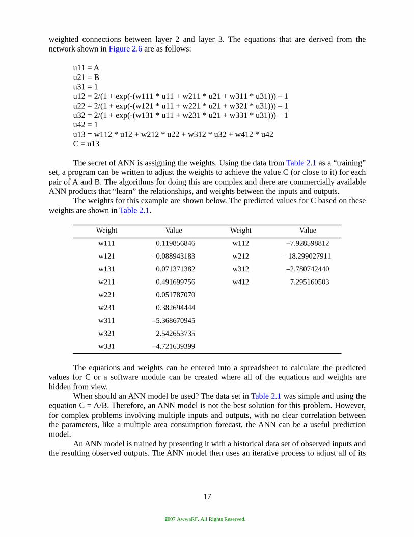
weighted connections between layer 2 and layer 3. The equations that are derived from thenetwork shown in Figure 2.6 are as follows:
u11 = Au21 = Bu31 = 1u12 = 2/(1 + exp(-(w111 * u11 + w211 * u21 + w311 * u31))) – 1u22 = 2/(1 + exp(-(w121 * u11 + w221 * u21 + w321 * u31))) – 1u32 = 2/(1 + exp(-(w131 * u11 + w231 * u21 + w331 * u31))) – 1u42 = 1u13 = w112 * u12 + w212 * u22 + w312 * u32 + w412 * u42C = u13
The secret of ANN is assigning the weights. Using the data from Table 2.1 as a “training”set, a program can be written to adjust the weights to achieve the value C (or close to it) for eachpair of A and B. The algorithms for doing this are complex and there are commercially availableANN products that “learn” the relationships, and weights between the inputs and outputs.
The weights for this example are shown below. The predicted values for C based on theseweights are shown in Table 2.1.
The equations and weights can be entered into a spreadsheet to calculate the predictedvalues for C or a software module can be created where all of the equations and weights arehidden from view.
When should an ANN model be used? The data set in Table 2.1 was simple and using theequation C = A/B. Therefore, an ANN model is not the best solution for this problem. However,for complex problems involving multiple inputs and outputs, with no clear correlation betweenthe parameters, like a multiple area consumption forecast, the ANN can be a useful predictionmodel.
An ANN model is trained by presenting it with a historical data set of observed inputs andthe resulting observed outputs. The ANN model then uses an iterative process to adjust all of its
Weight Value Weight Value
w111 0.119856846 w112 –7.928598812
w121 –0.088943183 w212 –18.299027911
w131 0.071371382 w312 –2.780742440
w211 0.491699756 w412 7.295160503
w221 0.051787070
w231 0.382694444
w311 –5.368670945
w321 2.542653735
w331 –4.721639399
17
©2007 AwwaRF. All Rights Reserved.

neuron input weights to minimize the total error between model outputs and observed outputs.After the training process, the ANN model can be applied as long as:
• Physical conditions do not change, affecting the actual relationship between inputs andoutputs
• The range of any input does not exceed the range of inputs used in model training
Most ANN model configurations used in consumption forecasting applications usuallyconsist of an input layer, one hidden layer and an output layer. The number of outputs correspondto the number of days forecasted into the future. Inputs would be selected by reviewing historicaldata to identify the most important variables which affect consumption. A typical template forinput variable choices might include:
• Forecasted temperature for one or more days, depending on the number of daysforecasted into the future
• Forecasted rainfall for one or more days, again depending on the number of daysforecast
• Other forecasted weather variables including humidity, dew point, wind speed, solarradiation
• Rainfall history for up to 7 days in the past• Temperature history for up to 7 days in the past• Daily consumption history for the last seven days • Seasonal parameters like season of the year, month of the year, day of the year• Calendar variables like day of the week, major holidays
Actual input variables to use in the ANN depend on the unique consumption patterns ofthe water utility’s customers.
JEA in Jacksonville, Florida, implemented an ANN consumption forecast model whichpredicts consumption for a number of operating areas in the water system called Subgrids. TwoANN forecasting models are used, one to forecast daily total consumption and one to forecasthourly consumption. Figure 2.7 shows actual daily versus forecast consumption for the RidenourSubgrid. JEA’s model inputs are:
• 7 Days of Hourly Average Flow History• Average Flow Over Period of 1 to 7 Days• 3 Days of Hourly Temperature History• 2 Days of Hourly Temperature Forecast• 4 Days of Hourly Relative Humidity History• 2 Days of Hourly Relative Humidity Forecast• 2 Days of Hourly Dew Point History• 2 Days of Hourly Dew Point Forecast
Artificial Intelligence—Expert System (Rule-Based) Techniques
Expert Systems have also been investigated for consumption forecasting and other engi-neering applications like process troubleshooting. Expert Systems analyze information and produce
18
©2007 AwwaRF. All Rights Reserved.

results by processing inputs through a series of questions, or rules. The answer to each questionpresents the next appropriate questions. Expert Systems are best visualized as a decision tree.
The series of questions and answers encoded into an Expert System are based on theknowledge, judgment and experience of human experts in the field. In a consumption forecastingapplication, water system operators would be the human experts, and the foundation of the fore-casting application would come from their heuristic knowledge of consumption behavior underdifferent conditions.
Expert System forecasting models have been evaluated in the water utility industry. Jainand Ormsbee (2002) implemented an Expert System application to forecast daily water consump-tion at Lexington, Kentucky. They developed the expert system rule set by observation of histor-ical consumption and discussions with water system operators. This resulted in the followingrules:
• If water consumption is below a threshold value, consumption on the next day will notchange significantly. This accounts for winter consumption periods.
• If water consumption is above a threshold value, and it does not rain today or the nextday, consumption on the next day will increase as a function of today’s consumptionand temperature. This accounts for dry periods during the summer.
• If water consumption is above a threshold value, and it rained yesterday and/or today,consumption on the next day will decrease as a function of consumption today andamount of rainfall yesterday and today. This accounts for rainy periods during thesummer.
Jain and Ormsbee (2002) incorporated these rules into two simple expert system modelswith a forecasting accuracy of 5–6% AARE.
Similar Day Technique
The basis for similar day forecasting rests on a relatively long-term historical database ofconsumption, weather data and other factors that make up a “similar day.” A forecast is made bysearching this database for days that closely match previous demands, day of week, season, fore-casted temperature, etc. Similar day forecasting has been used by electric and gas utilities. Itrequires an extensive and consistent historical record 4–5 years in length. This type of record isdifficult to obtain for most water utilities.
Heuristic Technique
The heuristic forecast is prepared by an “expert” in the utility who understands the day-to-day consumption patterns of the utility. This expert is often found in operations, a water systemoperator, or in strategic planning.
In the Operations environment, a senior operator or manager typically estimatestomorrow’s daily forecast based on today’s weather conditions and tomorrow’s forecast. Mainte-nance activities and pumping schedules are based on this consumption forecast. This forecast isbased on knowledge and experience with few, if any, computer based tools. An hourly forecast istypically based on a 24-hour consumption profile which is biased up or down based onyesterday’s consumption, recent historical trends, and tomorrow’s forecast.
19
©2007 AwwaRF. All Rights Reserved.

The accuracy of a heuristically prepared forecast can be very good as indicated in the datapresented later in the report. Daily AARE’s of the five prototype systems averaged 3.5%. The costis low considering the heuristic forecaster performs many other duties associated with operationsand maintenance of the utility. The heuristic forecast will work well for many applications such astreatment plant production scheduling. However, the feasibility of the heuristic forecast dimin-ishes when hourly forecasts are required every day for multiple consumption zones in the watersystem to support optimized pump scheduling. In that case, a computer-based forecast model isrequired. However, consumption forecasting is an art as much as a science and the heuristiccomponent is required to build, calibrate, and maintain any computer-based model.
Combination Techniques
Often the most effective forecasting strategy uses a combination of several techniques.Many large scale electric consumption forecasting applications combine regression, expert systemand ANN models into one larger application. The Expert System component makes decisionsabout which tool to use for various conditions.
Large forecasting applications will include decision-making elements. Many of the factorsaffecting water consumption are inherently discrete yes/no events. This is particularly true if theutility has lawn watering rules and restrictions in place, and the forecasting model must take theminto account. Some calendar-based factors like consumption changes due to major holidays alsolend themselves to a yes/no decision making algorithm. These considerations mean that waterconsumption models must incorporate rules. The rules are established with experience and knowl-edge of utility consumption patterns.
HOURLY CONSUMPTION FORECASTING METHODS
Common hourly consumption forecasting methods are:
• Standard hourly profiles for disaggregating the daily forecast• Previous day’s hourly profile or hourly profile from a week ago• ANN model producing an hourly forecast• Regression• Hourly time series model
Standard Hourly Profile Techniques
This method uses historical consumption data to develop typical hourly profiles fordifferent circumstances; usually based on day of week, weekday vs. weekend, major holidays,winter vs. summer, etc. The hourly profiles are similar to the example shown in Figure 2.2, exceptthat all profiles are normalized by dividing each day’s 24 hourly average consumption values bydaily total consumption for that day. These normalized profiles are more convenient for compari-sons between different days, and make it easy to generate an hourly forecast from the daily totalforecast.
Once the standard hourly profile set is developed, generating an hourly forecast is a simpleprocess. A decision making algorithm selects the standard profile for current conditions and theapplication multiplies daily total forecast by the standard profile values.
20
©2007 AwwaRF. All Rights Reserved.

Previous Day Techniques
This method assumes that a normalized hourly profile from a previous day, typicallyyesterday or one week ago, is a good representation of the upcoming hourly profile. Again, thehourly forecast is simple. Call up the previous day normalized profile and multiply it by the dailytotal consumption forecast.
Hourly ANN Model Techniques
Using an ANN model to produce hourly forecasts is common in both the electric andwater utility industry. The two ANN applications previously defined produce both hourly anddaily forecasts.
Regression
A regression model first estimates daily consumption and then estimates how that flowwas distributed across the day. Several weeks of historical data are used to estimate daily andhourly consumption.
Time Series Modeling Techniques
This method uses mathematical and statistical techniques to model the diurnal hourly usepattern. Modeling the diurnal curve as a Fourier series is one commonly used method.
The simplest time series models just use season and day of week as variables for adjustingthe hourly profile. In a sense, these models are one level of sophistication above standard hourlyprofiles selected for season and day of the week.
More sophisticated hourly time series models include temperature and rainfall parametersto account for changes in the hourly profile due to weather conditions.
FORECASTING TECHNIQUES SELECTED FOR PROTOTYPING
Based on research on forecasting techniques, experience of the researchers, and review bythe Project Advisory Committee, it was decided to prototype Heuristic and ANN models at fiveutilities as defined in Chapter 5. Regression models were then added later as prototypes at TorontoWater and Washington Suburban Sanitary Commission. These short-term consumption fore-casting techniques were selected because of their popularity and successful results fromelectric/gas utilities, accuracy, cost, and ease of use in an operating environment.
Chapter 4 of the Report defines the experience of Colorado Springs, JEA, San Diego, andLas Vegas Valley Water District using Similar Day, ANN, and Regression techniques.
21
©2007 AwwaRF. All Rights Reserved.
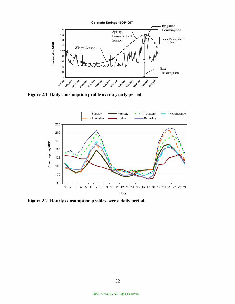
Figure 2.1 Daily consumption profile over a yearly period
Figure 2.2 Hourly consumption profiles over a daily period
Colorado Springs 1996/1997
0
20
40
60
80
100
120
140
160
180
/91
91/96
01/
6991/101/
6991/131
/13
1/099
6
1/23
1/099
6
1
7991/92/ 2
91/82/
97
/33
7991/0
7991/92/4 5 2/9/
1997
6 2/8/
1997 7991/82/7
7991/72/8
Spring,Summer, Fall Season
Winter Season
Base Consumption
Irrigation Consumption
ConsumptionBase D
GM noitp
musnoC
/ /
79 991/92/4 6/
91
2
DM
50
75
100
125
150
175
200
225
1 2 3 4 5 6 7 8 9 10 11 12 13 14 15 16 17 18 19 20 21 22 23 24
Sunday Monday Tuesday Wednesday
Thursday Friday Saturday
Co
nsu
mp
tio
n, M
GD
Hour
22
©2007 AwwaRF. All Rights Reserved.
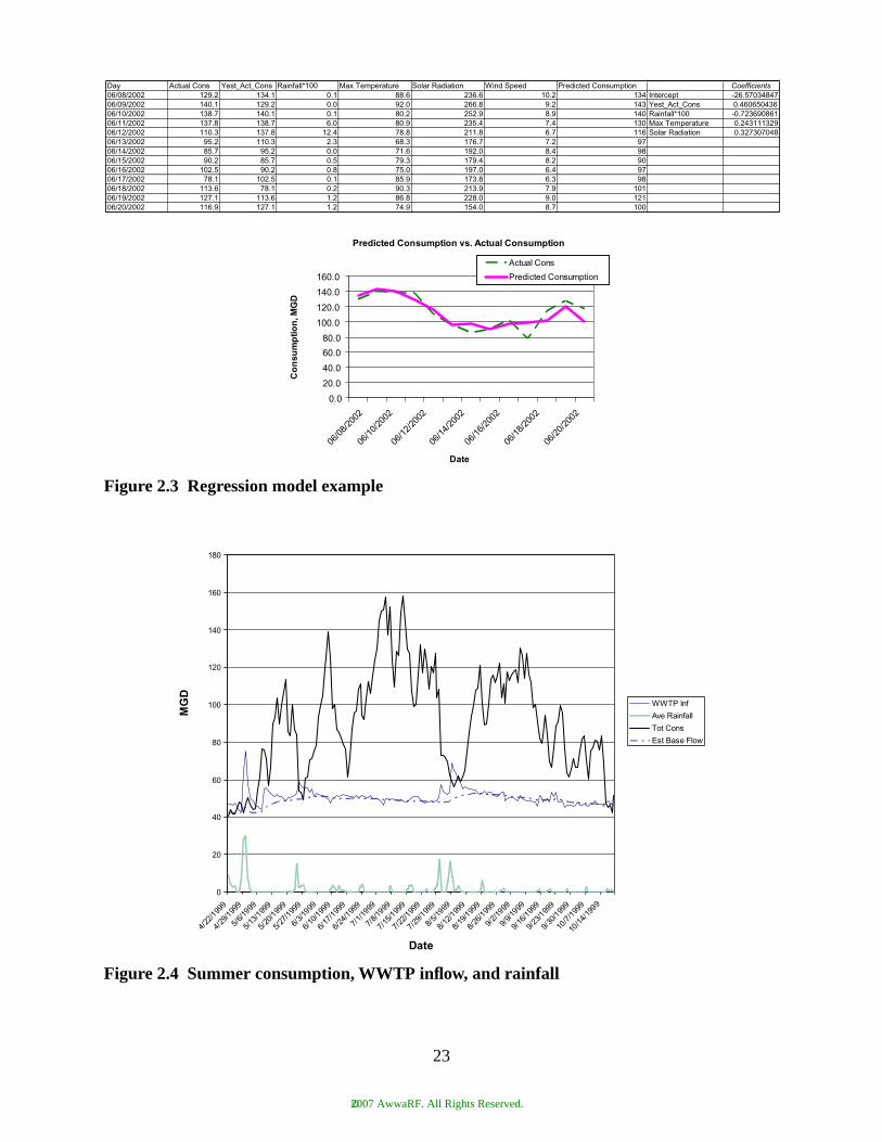
Figure 2.3 Regression model example
Figure 2.4 Summer consumption, WWTP inflow, and rainfall
Predicted Consumption vs. Actual Consumption
0.0
20.0
40.0
60.0
80.0
100.0
120.0
140.0
160.0
06/80/20
02/01/60
2002
/21/60
2002
/41/60
2002
1/606
2002/1/608
2002/
06/2
0
2002/
Date
DG
M ,n
oitp
mus
no
C
Actual Cons
Predicted Consumption
Day Actual Cons Yest_Act_Cons Rainfall*100 Max Temperature Solar Radiation Wind Speed Predicted Consumption Coefficients06/08/2002 129.2 134.1 0.1 88.6 236.6 10.2 134 Intercept -26.5703484706/09/2002 140.1 129.2 0.0 92.0 266.8 9.2 143 Yest_Act_Cons 0.46065043606/10/2002 138.7 140.1 0.1 80.2 252.9 8.9 140 Rainfall*100 -0.72369086106/11/2002 137.8 138.7 6.0 80.9 235.4 7.4 130 Max Temperature 0.24311132906/12/2002 110.3 137.8 12.4 78.8 211.8 6.7 116 Solar Radiation 0.32730704806/13/2002 95.2 110.3 2.3 68.3 176.7 7.2 9706/14/2002 85.7 95.2 0.0 71.6 192.0 8.4 9806/15/2002 90.2 85.7 0.5 79.3 179.4 8.2 9006/16/2002 102.5 90.2 0.8 75.0 197.0 6.4 9706/17/2002 78.1 102.5 0.1 85.9 173.8 6.3 9806/18/2002 113.6 78.1 0.2 90.3 213.9 7.9 10106/19/2002 127.1 113.6 1.2 86.8 228.0 9.0 12106/20/2002 116.9 127.1 1.2 74.9 154.0 8.7 100
0
20
40
60
80
100
120
140
160
180
9991/22/4
9991/92/4/6/5
9199
/5/311
999/02/5
1999/72/5
1999/3/6
9199
1/01/6
999
/6/711
999/42/6
1999
9991/1/7/8/7
9199 9991/51/7
1/22/7
999
/7/921
9999991/5/8/21/8
1999
9991/91/8
9991/62/8/2/9
99919991/9/9/61/9
1999
9991/32/9
9991/03/9
1/7/01
999/41/01
9919
Date
DG
M
WWTP Inf
Ave Rainfall
Tot Cons
Est Base Flow
23
©2007 AwwaRF. All Rights Reserved.
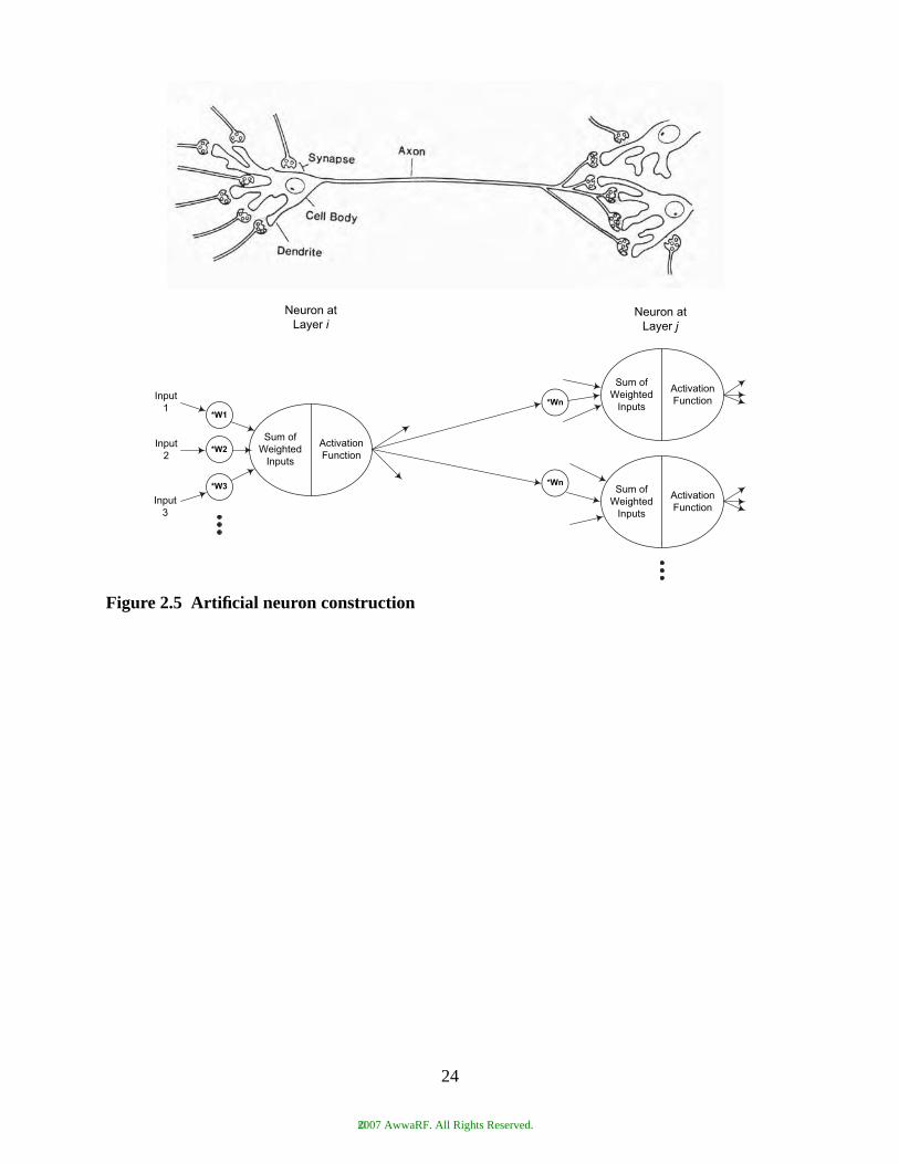
Figure 2.5 Artificial neuron construction
Sum of Weighted
Inputs
Input1
*W1
Activation Function
Input 2
*W2
Sum of Weighted
Inputs
ActivationFunction
Sum of Weighted
Inputs
ActivationFunction
*Wn
Input3
*W3
Neuron at Layer i
Neuron at Layer j
*Wn
24
©2007 AwwaRF. All Rights Reserved.
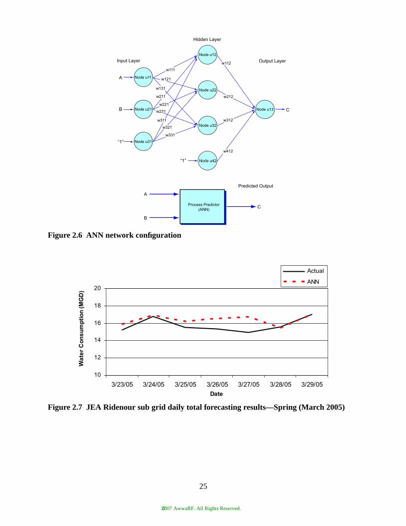
Figure 2.6 ANN network configuration
Figure 2.7 JEA Ridenour sub grid daily total forecasting results—Spring (March 2005)
A
A
B
B
C
C
“1”
“1”
Input Layer
Hidden Layer
Output Layer
Predicted Output
Node u11
Node u12
Node u13
Node u22
Node u32
Node u42
Node u21
Node u31
w111
w121
w131
w211
w221
w231
w311
w321
w331
w312
w212
w112
w412
Process Predictor(ANN)
10
12
14
16
18
20
3/23/05 3/24/05 3/25/05 3/26/05 3/27/05 3/28/05 3/29/05
Date
)D
GM(
noit
pm
us
no
C ret
aW
Actual
ANN
25
©2007 AwwaRF. All Rights Reserved.

©2007 AwwaRF. All Rights Reserved.

CHAPTER 3STCF DEVELOPMENT PROCEDURES
This chapter presents a brief description of a process used to select, configure, test andimplement a consumption forecasting application.
FORECASTING APPLICATION DEVELOPMENT OVERVIEW
Figure 3.1 is a flow chart of a typical forecasting application development process.This process begins by defining the application requirements for the forecaster. The service
area and any sub-areas to be covered in the forecast are defined. The next steps involve gathering,assembling and analyzing historical consumption and weather data for the service area(s).
The analysis phase concludes with a description or definition of the key patterns and asso-ciated drivers that characterize consumption in the service area. This is the basis for selecting theappropriate forecasting technique and configuring the associated forecasting model.
Once the forecasting model is configured, the next phase is to calibrate the model parame-ters or train the ANN, until the fit between observed and forecasted consumption is within accept-able limits. If possible, the calibrated model is then verified against a different data set than wasused for calibration. An alternative is to run the model for a period of time with “real-time” oper-ating data and track model forecasting error. Results of the verification step provide the expectedAARE and error distribution for the production forecasting application. If these values are notacceptable, different modeling techniques and/or model formulations should be investigated.
In an operations environment, the forecasting model is integrated with a user interface andother applications, run on a daily basis, monitored for accuracy, and modified if accuracy fails tobe within acceptable limits.
The following paragraphs describe the consumption development steps in more detail, upthrough and including the model verification step.
Define Forecasting Requirements
The first step is to define the applications that will use the output of the forecaster. It isimportant to clearly define the applications that will use the consumption forecast. Data needs ofapplications such as energy cost minimization and water treatment plant scheduling will drive thespecifications for the forecaster. Accuracy, number of service areas, sensitivity factors and type ofmodel are attributes which are developed based on the projected use of the forecaster.
Identify the Service Area
For pump control, it is important to formally define the service area(s) requiring a forecastand begin gathering the required data. Figure 3.2 shows an example service area to illustrate theseconcepts.
The first step is to develop a water system schematic as shown in Figure 3.2. The sche-matic is used to delineate service area boundaries, and the boundaries of any sub-areas that will bebroken out of the main service area.
27
©2007 AwwaRF. All Rights Reserved.

The next step is to identify all water system facilities that put water into or transfer waterout of the service area. Types of facilities include water treatment plants, wells, pumping stations,flow transfer valves, pressure regulating valves, etc. Also identify all water storage reservoirswithin the service area.
This stage of the development process is also the best time to gather the necessary infor-mation about water system facilities. For water treatment plants define and identify maximum andminimum treatment capacity and treated water flows. For pumping stations or wells, define andidentify the source for total station flow capacity, number of pumps, and horsepower and flowrating of each pump. For valve sites, identify and define the source for total site flow transfercapacity, number of valves, and type, size and capacity of each valve. For storage reservoir sites,define and identify the type of site (elevated vs. ground), reservoir volume, reservoir depth, eleva-tion of the reservoir overflow, and the reservoir’s depth to volume relationship.
Facility information is necessary to develop an understanding of how the water systemoperates. The flow, reservoir volume and level information is required to estimate historicalconsumption in the service area.
This initial information gathering step is also critical in identifying missing informationthat may prevent further work until the information is available, or acceptable work-a-rounds areidentified. Un-metered flows into or out of the service area are the most common problem.
Gather Historical Data
Once the service area is defined, the next step is to gather the historical data needed toquantify historical consumption, examine consumption trends in conjunction with significantweather data like temperature and rainfall trends, and calibrate and verify the forecasting model.
A minimum of two years daily and hourly consumption data are typically required todevelop a good forecasting model. Daily and hourly consumptions for the service area are typi-cally calculated based on total flow into, total flow out of, and change in total reservoir storagevolume over each hourly and daily period. This is where the flow meter and reservoirlevel/volume data are required. It is best to obtain hourly data, which can be used to calculate bothdaily and hourly consumption.
Daily weather data for the relevant time period is usually sufficient. Hourly weather data ishelpful if it can be obtained. Daily total rainfall, maximum daily temperature, minimum dailytemperature and average daily temperature are often required. Other useful daily weather dataincludes degree of cloudiness (or actual total daily solar radiation readings if available), averagewind speed and direction, humidity, relative humidity, etc.
Data from more than one weather monitoring site should be obtained if possible. Data fromweather monitoring sites in and surrounding the service area should be examined to find the site—or combination of sites—where weather parameters correlate most closely with consumption.
Assemble the Data Set
After the base historical data set is gathered, it must be assembled into a form that can beused for the rest of the model development process. A database application is usually the mostconvenient way to handle the large amounts of data.
The first step is evaluating the base historical data to identify missing data and/or dataoutliers. If blocks of data are missing, the model developer must find out if it can be backfilled by
28
©2007 AwwaRF. All Rights Reserved.

some reasonable method, or decide if the periods with missing data should be excluded from theanalysis. Also, if the base data set contains outliers or obviously bad values, the model developermust decide if these data points can be adjusted by some reasonable method, or should beexcluded from the analysis. The model developer should evaluate both the base operational dataand the base weather data.
After the base historical data set has been evaluated and “groomed,” the next step is toperform the estimated consumption calculation. These estimated consumption results must alsobe evaluated for outliers. Since the base data set was groomed prior to the consumption calcula-tion, there is a high likelihood that the outlying consumption values are real, and the result ofsome unusual event. The model developer must consult with the water system operators to try andidentify the reason for the outlying consumption points. Based on this, the model developer mustthen decide if the outlying consumption points should be excluded from the analysis.
After these data verification steps, the data set is ready for the actual model developmentsteps.
Analyze the Data for Correlations
After a clean historical record of consumption and weather is available, the actual modeldevelopment process begins. The first thing to do is to identify the factors that affect consumptionin a statistically similar way. These factors will become the forecasting model inputs.
It is usually best to start by examining the consumption trend against the primary weatherfactors temperature and rainfall. This gives the model developer a chance to identify the importantconsumption phenomena described in Chapter 2. It also gives the developer a feel for theconsumption response patterns of the particular service area under evaluation.
The next step is to perform a statistical correlation analysis between what appear to be thekey driving events and observed consumption. This should confirm the responses that show up viavisual analysis. The statistical analysis often includes auto-correlation which identifies correla-tions between the current day’s data and previous day’s data. Auto-correlation helps to identifywhether or not the previous day’s events significantly affect today, and also help to identify signif-icant weekly patterns.
Note that ANN packages often include tools to help perform these statistical analyses.Other specialized statistical analysis packages are available, or the calculations can be performedwith standard spreadsheet tools.
This step should result in a list of the input variables for the forecasting model.
Formulate the Model
At this point, the model developer must make a final decision about what forecasting modeltechnique would be best for the current application, and decide how the resulting forecasting modelshould be formulated. This decision can wait to this point, because all of the previous steps have tobe performed no matter what modeling technique the model developer uses.
The forecasting model’s construction will depend on the selected modeling technique. Thefollowing is a list of some of the decisions involved:
• Make the final selection of model input variables. Only use input variables proved tobe significant during correlation analysis. When in doubt, use fewer variables rather
29
©2007 AwwaRF. All Rights Reserved.

than more, at least for the first cut. Remember that many forecasting models achieveadequate performance using only past consumption, temperature and rainfall as inputs.
• If applicable, make the final selection of model output variables.• For time series-type models, make the final selection of the transfer functions used to
model the time series.• For an ANN-type model, decide if there should be more than one hidden layer.• For an Expert System-type model, formally define the model decision questions.
After the appropriate decisions are made, the model developer can configure (program)the forecasting model.
Calibrate (Train) the Model
Once the forecasting model has been formulated and configured into the model tool, thenext step is to adjust model parameters until the model forecasts match observed values with aminimum of error. This process is called model calibration. Or in the case of an ANN-type model,it is called model training.
Calibration is an iterative process that can be very time consuming. The model developerhas to use a systematic method of adjusting model parameters one at a time and keep track ofwhich combination of parameters work best. The model developer should use Average AbsoluteRelative Error (AARE) and error distribution to guide parameter adjustments and decide when themodel is sufficiently calibrated.
ANN-type models provide an advantage during calibration, because they have built-intools to automate the training process. ANN models store all of the connection weights in aninternal database, and use an optimization routine to iteratively zero in on the combination ofconnection weights that minimizes total overall error.
When the forecasting model has been calibrated, it is ready for testing. This is called themodel verification step.
Verify the Model
The model verification step is the final model test before placing it into operation. The bestway to do this is to use a separate data set that is independent of the data set used for calibration.The model is run using this verification data set, and forecasts are compared against actualobserved consumption. The errors between actual and forecast consumptions are processed togenerate the AARE and error distribution. If AARE and error distribution fall within acceptablelimits, the forecast model is ready to go into operation.
Some utilities may not have a long enough or consistent enough historical data set to allowa separate historical data set for verification. If this is the case, the forecasting model should beverified by running it on-line in real-time. The model errors can be processed to track AARE anderror distribution over time. Note that on-line verification may take 12 months or more becausethe forecaster should be evaluated for every possible seasonal condition.
30
©2007 AwwaRF. All Rights Reserved.

Integrate the Model
After the model is calibrated, it can be integrated with the operations applications that usethe STCF. This may be other software applications or human processes which will use the fore-caster for operations planning and scheduling.
Evaluate Performance
To insure the STCF remains in calibration during operation, it is necessary to measureperformance daily, or in the case of real-time applications—hourly. When actual consumptioncompared to the forecast exceeds a specified dead band, alarms or alerts should be generated toalert the operations planner that the forecast error is excessive and appropriate measures should betaken. For real-time adaptive applications, a new forecast may be generated automatically.Consistent high error rates should trigger the need to analyze and potentially recalibrate the STCF.
EVALUATION CRITERIA
Short-term consumption forecasting can be a highly technical process involving sophisti-cated mathematical and statistical techniques. Because of this, there may be a tendency to focusonly on the statistical accuracy or mathematical elegance of different forecasting methods. Obvi-ously accuracy is critical and must be considered in any evaluation. Mathematical elegance isnice, but in the end, these forecasting applications must be maintained in an operations environ-ment. With this in mind, cost of maintenance and ease-of-use are important considerations.
The software tools needed to implement the forecasting model are another importantconsideration. Software tools affect initial cost of the application, amount of time and effortrequired to learn the application, and amount of time and effort required to maintain the applica-tion on an ongoing basis.
Based on the discussion above, this preliminary evaluation uses the following criteria:
• Accuracy—How well do forecasted values match actual values as measured by theAARE parameter?
• Implementation complexity—How complex is the mathematical and statisticalknowledge required to set up and configure the application?
• Ease of maintenance—What is the level of complexity and time required evaluatemodel performance and update the model when necessary?
• Tools required—What types of software tools are required to implement theapplication? How difficult will they be for water utility personnel to learn and use?
EVALUATION OF DAILY FORECASTING METHODS
As previously stated, selection of the forecasting methodology depends on a number offactors. This section of the report defines advantages and disadvantages of each type of model.
Note that all forecasting methods require some type of database tool to help assemble andanalyze the historical data needed for application design, calibration and testing. The same data-base tool can be used for ongoing performance evaluation and model re-calibration as necessary.
31
©2007 AwwaRF. All Rights Reserved.

Regression Models
The electric utility industry has had good success with regression models for forecastinghourly electric consumption. The prototype regression models developed in this study performedwell.
Regression models can be difficult to implement. Once the regression equations aredefined, the regression parameters can be easily obtained using standard spreadsheet tools, orother statistical software packages. However, because water consumption is an inherently non-linear process, the regression parameters change with season, day of week, weather, andconsumption levels. To compensate, different regression models are often defined and calibratedfor different conditions and circumstances. The amount of effort required to calibrate and main-tain the application increases exponentially as the number of regression equations increases.
Regression models are also difficult to maintain over time. As discussed above, the regres-sion parameters and appropriate regression equation change as conditions change. This can takeconsiderable time, especially if there are various regression models for different conditions.Regression models do not require special tools. They can be implemented with standard databaseand spreadsheet tools that most water utility personnel are familiar with. This tends to keep theinitial cost of the model low and reduces the training requirements for utility personnel.
Time Series Models
Time series models can be quite accurate. However, time series models can be difficult toimplement. The mathematical and statistical basis of time series models is complex, althoughadvanced statistical analysis packages are available to help simplify time series model develop-ment. Time series models typically require many different parameters, which can cause the cali-bration process to be time consuming, and management of those parameters challenging. Modelparameters are often obtained by non-linear regression, which can be difficult.
Because of their complexity, time series models are difficult to maintain over time. Aswith regression models, the model parameters change over time as conditions change, requiringperiodic recalibration. Water utility personnel responsible for maintaining the forecasting modelwill require training in the model’s mathematical and statistical basis, and in the computationaltools used to develop and implement the model. Even if the model is implemented on standardspreadsheet tools, model users need to be familiar with the special statistical functions used. Aspreviously discussed, time series models have many parameters, which makes parameter mainte-nance difficult and time consuming.
On the other hand, time series models can generally be implemented using standard data-base and spreadsheet tools. Like the regression models, the initial cost can be low. However, timeseries models may have a higher training requirement because of the complexity.
Statistical software packages can reduce the time and effort required to implement andmaintain a time series model, but these software packages add to the initial cost of installation.
ANN Models
Experience in the electric and gas industries, have shown ANN models to be quite accu-rate. The ANN models analyzed in this study performed well considering the labor expended incalibration and maintenance.
32
©2007 AwwaRF. All Rights Reserved.

Experience with recent ANN forecasting implementations and the prototypes developedon this project have shown that the effort required to implement an ANN model is generally lessthan a comparable regression or time series model. This is because model developers and usersdon’t have to understand the underlying mathematics of an ANN engine to effectively use it. Also,most ANN engines come with built-in analysis tools that help users select appropriate inputparameters and navigate the model training process.
ANN models do not require calibration in the same sense as regression and time seriesmodels, but they do undergo a training process. Training does take time. However, once thetraining data set is organized, it is possible to evaluate several alternative ANN model formula-tions in a short time, which helps model developers and users quickly identify the most effectiveANN model.
Another advantage of an ANN model is that the ANN tool manages the model parametersinternally, taking this burden off of the user.
Long-term maintenance requirements for ANN models are less than that of comparableregression or time series models. However, most water utility personnel will require training inthe ANN tool.
The primary disadvantage of ANN models is that the ANN engine can be costly. Thisincreases the initial cost of an ANN model implementation.
Expert System (Rule-Based) Models
Developing a rule-based model is moderately difficult. Rule-based models do not requiresophisticated mathematics and statistics, but they do require model developers to spend time eval-uating historical data and interviewing water system operators, understanding the key things thatdrive consumption variations, and distilling them into a set of rules that can be implemented witha computer algorithm.
Long-term maintenance requirements for rule-based models are moderate as well. Thisinvolves keeping track of water system conditions and updating the model as the rules change.
Expert System tools are available to simplify implementation of a rule-based model. Themain advantage of an Expert System tool is in simplifying the process for encoding, storing andupdating the rules. Using an Expert System tool increases the initial cost of the application soft-ware, but reduces the cost of model configuration and long-term maintenance.
Combined Models
Combined models may be more accurate than using a single forecasting method. Experi-ence of electric and more sophisticated water utilities supports this statement. For example, Jainand Orsmbee chose to combine rule-based decision-making with an ANN model. However, rulesand heuristics are combined with ANN and regression techniques.
Adding additional rules to any of the forecasting methods previously discussed willincrease implementation effort, and is likely to increase the long-term maintenance effort as well.This is because both the forecasting model (possibly multiple models for different conditions) andthe associated rules need to be configured and updated as conditions change.
A combined model will also add to initial cost of the model implementation, becausesome method of automatically executing the rules in conjunction with the forecasting model, or
33
©2007 AwwaRF. All Rights Reserved.

models, will be required. An Expert System software package may be required depending on thecomplexity of the rules involved.
PROTOTYPE RECOMMENDATIONS
If time and budget were not an issue, the research team for this project would have evalu-ated and tested each of the forecasting model types at every utility in this study. Unfortunately,time and budget were limitations. This study focused on the most promising forecasting tech-niques based on the previously defined research.
This study prototyped and tested the following short-term forecasting techniques.
1. ANN Models—ANN techniques have a good balance of high accuracy and moderateimplementation and maintenance requirements. Their chief drawback is cost of theANN engine. This selection was also made on the observation that electric and gasutilities currently favor ANN models based on operational experience.
2. Regression Models—Regression models can be developed using off-the-shelf soft-ware and database tools. As with the ANN recommendation, regression techniques arefrequently used by electric utilities. The primary issue is the maintenance cost whereconsumption forecasts are required in multiple operating areas.
3. Heuristic—Forecasts are developed with the use of a seasonal and day-of-the-weekhourly consumption profile adjusted up or down considering the experience of theoperations planner or operator. This is the least expensive initial cost method, butrequires a skilled operations planner. It would be very time consuming and difficult toimplement if forecasting is required on an hourly basis for multiple operating areas.However, if applications for a consumption forecast only require a daily forecast forthe system, this is an attractive approach.
Two to three methods were selected for prototyping and evaluation at each of the partici-pating utilities who were currently not forecasting consumption (Toronto, WSSC, EBMUD, SPU,GVRD). Selection was based on factors such as the application for the forecaster, data availability,consumption patterns and staff preference.
Role of the Operator/Operations Planner in Consumption Forecasting
Even with an automated consumption forecasting application, there is no real substitutefor operations knowledge, experience and intuition. This was confirmed in the prototype work forthis project.
No forecasting method is perfect, and there will always be unusual events that put watersystem conditions outside of the forecasting model’s calibration zone. For this reason, consump-tion forecasts should be reviewed before they are released to applications. Or, the applications willrequire adaptive measures to automatically correct for actual conditions which significantlydeviate from the forecast.
34
©2007 AwwaRF. All Rights Reserved.
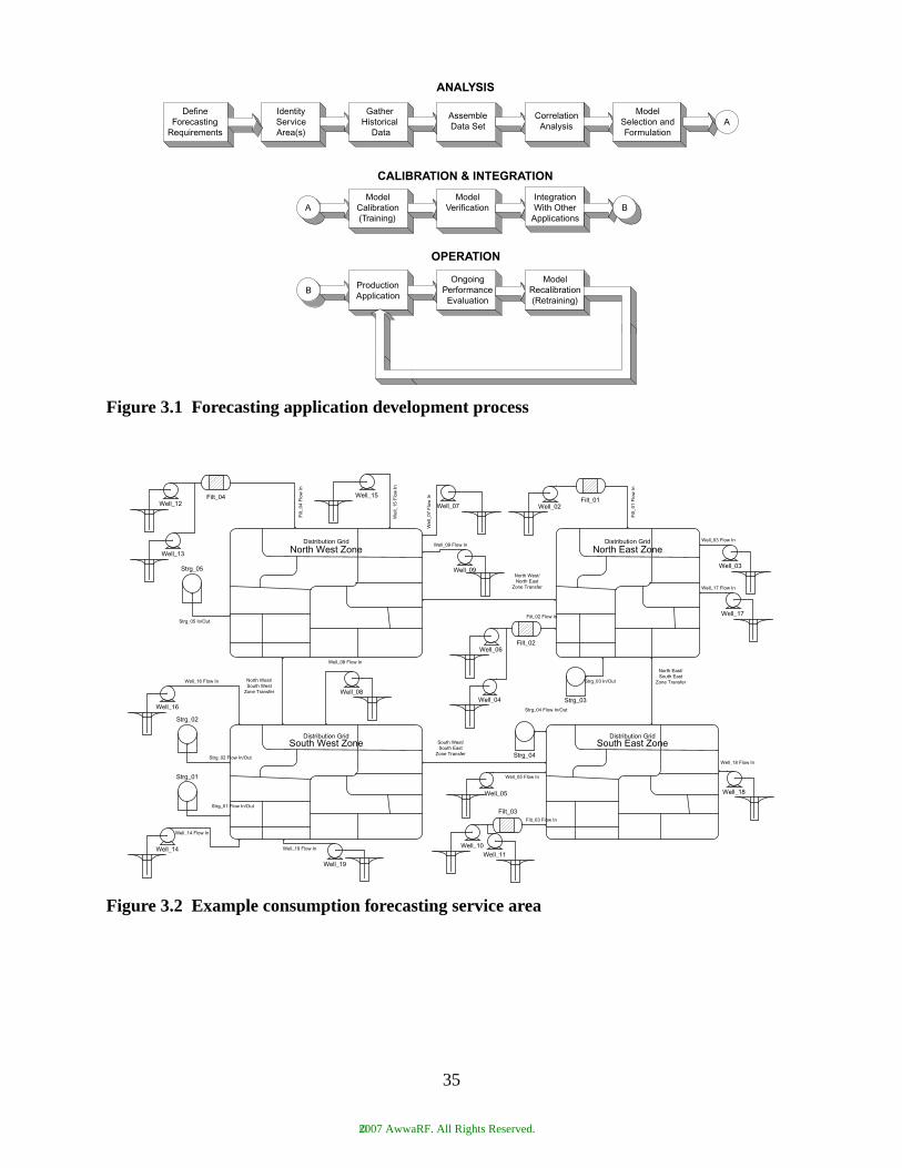
Figure 3.1 Forecasting application development process
Figure 3.2 Example consumption forecasting service area
DefineForecasting
Requirements
IdentityServiceArea(s)
Gather Historical
Data
AssembleData Set
CorrelationAnalysis
ModelSelection andFormulation
ModelCalibration(Training)
ModelVerification
IntegrationWith Other
Applications
ProductionApplication
OngoingPerformanceEvaluation
ModelRecalibration(Retraining)
A
A
B
B
ANALYSIS
CALIBRATION & INTEGRATION
OPERATION
Well_12
Well_13
Filt_04
nI wol
F 40_tliF
Strg_05
Strg_05 In/Out
Well_15
Well_07
Well_09
nI wol
F 51_lle
W
nI wol
F 70_lleW
Well_09 Flow In
Strg_03
Distribution Grid
North East Zone
Well_06Filt_02
Filt_02 Flow In
Strg_03 In/Out
North West/North East
Zone Transfer
Well_04
Well_17
Well_17 Flow In
Well_03
Well_03 Flow In
Well_02Filt_01
nI wol
F 10_tliF
Distribution GridSouth East Zone
Distribution GridSouth West Zone
Strg_04
Strg_04 Flow In/Out
Well_10
Filt_03Filt_03 Flow In
Well_11
Well_05
Well_05 Flow In
Well_18
Well_18 Flow In
South West/South East
Zone Transfer
North East/South East
Zone TransferNorth West/South West
Zone Transfer Well_08
Well_08 Flow In
Strg_02
Strg_02 Flow In/Out
Strg_01
Strg_01 Flow In/Out
Well_16
Well_16 Flow In
Well_14
Well_14 Flow In
Well_19
Well_19 Flow In
Distribution Grid
North West Zone
35
©2007 AwwaRF. All Rights Reserved.

©2007 AwwaRF. All Rights Reserved.

CHAPTER 4ANALYSIS—EXISTING STCF SYSTEMS
INTRODUCTION
This section of the report provides information on operational STCF systems at JEA,Colorado Springs Utilities, San Diego Water Department and Las Vegas Valley Water District.These utilities provide good diversity in climatic conditions and customer demographics. TheSTCF tool used at each utility is listed below:
JEA
JEA is a multi-service utility providing potable water, wastewater, and electric service to apopulation of approximately 800,000 people in the Jacksonville, Florida area (Figure 4.1).
The JEA water system is a ground water source system. The ground water supply is fromthe Floridan Aquifer and is delivered using well fields, reservoirs for storage and high servicepumps for delivery. There are a total of 39 plants and 138 wells within the total system whichdeliver approximately 121 million gallons daily. There are 3,400 miles of distribution mains in theJEA water delivery system. The JEA water system is physically separated by the St. Johns Riverinto a North Grid distribution system and a South Grid distribution system with various othersatellite facilities in St. John’s and Nassau Counties.
The North Grid system consists of 10 water treatment plants and 49 wells. The South GridSystem consists of 18 water treatment plants and 67 wells.
Water is pumped from the Floridan aquifer through aerators on each reservoir for hydrogensulfide stripping. Water is then pumped into the distribution system and chlorinated as it leaves theplant. Currently, 72 reservoirs located at water treatment plants have a combined capacity of71 million gallons of water. Pressure is normally maintained at each water treatment plant between70 and 80 psi via high service pumping. There are no elevated storage tanks in the distributionsystem. Distribution system pressure is maintained by the high service pumps at the plants.
STCF Requirements
The primary purpose of the JEA Water Consumption Forecaster (WCF) is to forecastwater consumption for each sub grid (or consumption point) in the JEA South Grid. JEA uses anArtificial Neural Network (ANN) model for their STCF. An optimized pump schedule is gener-ated to meet forecasted consumption. Wells are scheduled to meet JEA’s Consumptive Use Permit(CUP), provide high quality water and minimize cost. This is achieved by optimally scheduling
Utility STCF Technique
JEA ANN
Colorado Springs Utilities Similar Day
San Diego ANN
Las Vegas Valley Water District Regression, ANN, Heuristic
37
©2007 AwwaRF. All Rights Reserved.

wells and high service pump stations in the South Grid. An accurate forecast is mandatory forsuccessful optimization.
The WCF is one of the ten modules developed in an Operations Optimization (OO)Project. The outputs of the forecaster are essential inputs to the Simulator, the Water SupplyAnalyzer, and the System Scheduler (Optimizer).
The WCF calculates a consumption forecast at a sub grid level. The Sought Grid is parti-tioned into sub grids according to the distribution system topology. Figure 4.2 shows the conceptof sub grid and consumption points.
A Treatment Plant supplies water to one sub grid or consumption point. Pumpage betweensub grids is assumed to be negligible.
Nine sub grids were defined in the South Grid. The WCF generates a 48-hour forecast foreach sub grid. The forecast resolution is hourly. The forecast is executed automatically atmidnight or by user command. An Optimization Monitor automatically initiates a new consump-tion forecast if the actual consumption significantly deviates from forecast. The revised forecastthen triggers the System Scheduler to develop a new pump schedule.
The WCF stores forecast results so previously generated forecasts can be recovered andreused. In the case that the WCF is not able to generate a forecast, the last successfully generatedforecast is recovered and reused.
The input to the WCF consists of the following:
• Seven days of hourly average flow history of each sub grid• Average flow over a period of one to seven days of each sub grid• Three days hourly temperature history and 48 hour forecast• Four days hourly relative humidity history and 48 hour forecast• Two days hourly dew point history and 48 hour forecast• Seven days of daily rainfall history and 48 hour forecast
Neural network models for each sub grid were initially trained using historical data. TheWCF input data is stored and used to retrain the neural network models online. Requirements forthe WCF are categorized as follows:
• Accuracy—The total daily forecast accuracy is 90% or better, with a goal of 95%. Thehourly average forecast accuracy is 85% or better, for 75% of the hours of the forecast.
• Resolution—Hourly • Distribution—Nine sub grids• Input Data—Historical consumption data from SCADA and weather data from an
Internet weather proxy.• Human Forecaster—Operations Planner Scheduler (OPS)• Optimization Dynamics—Pump schedule is developed once a day and run for the
entire day. OPS can initiate a new forecast at any time.• Weather Sensitive Consumption Parameters—air temperature, dew point, and rainfall.
STCF Experience
The initial step in development of the WCF model was to acquire historical consumptiondata from the SCADA system. Gaps and errors in the data were identified and corrected.
38
©2007 AwwaRF. All Rights Reserved.

Historical weather data was obtained from the National Weather Service for the same period asthe historical consumption data. Using the Neural Network modeling software, trends of the datawere examined to determine correlations between the consumption data and the weather data, aswell as other indicators. Air temperature, relative humidity, dew point and rainfall had good corre-lation with the consumption data. Wind speed, wind direction and wind gusts had little or nocorrelation. Other indicators, such as day of the week, also had little or no correlation.
Next, prototype models were developed to calibrate the model to find the best combinationof input parameters. The final model was then integrated with the Operations OptimizationSystem. Preliminary tests of the model were performed to verify accuracy of the model.
The WCF obtains operations data through an interface to the SCADA system. Outputresults of the WCF are passed automatically to the System Scheduler that creates the optimizedpump schedule for the SCADA System.
Lessons learned include the following:
• Data Quality is Important—Valid real time data are needed to provide accurateforecasts. In addition, valid historical data are required to correctly retrain the WCFmodel.
• Keep the Design Simple and Flexible—The model design should not use parametersthat are poorly correlated. The model needs to be simple and easy to modify.
• Keep the User in the Loop—The model is retrainable online, but the re-training is notautomatic. Automatic re-training is not used because consumption can be substantiallyaffected by short-term weather events and operational factors such as maintenance. Tokeep the model properly updated, the OPS reviews forecast accuracy and initiates there-training process when the accuracy has drift away from acceptable norms.
STCF Operational Performance
Data from the Ridenour Sub grid were collected for twenty-eight days, seven days fromeach season for analysis. Figures 4.3 to 4.10 are graphs of the hourly and daily forecasts andactual consumption for each season.
Extreme Weather
During the 2004 Hurricane Season, the Jacksonville area was affected by HurricaneJeanne. Over the three day period from September 25, 2004 to September 27, 2004 the averagewind speed was 18 mph with maximum wind speeds up to 35 mph. The average precipitationfrom September 24, 2004 to September 30, 2004 was 0.67 inches, with most of the precipitation,4.12 inches, occurring on September 27, 2004. Schools and a number of businesses were closed.Figures 4.11 and 4.12 illustrate STCF accuracy during the hurricane period.
Error Analysis
In general, the ANN forecast closely followed the actual consumption. Table 4.1 is asummary of the Average Absolute Relative Errors (AARE). Large errors in the forecast during thehurricane illustrate the need for intervention when an extreme weather event occurs.
39
©2007 AwwaRF. All Rights Reserved.
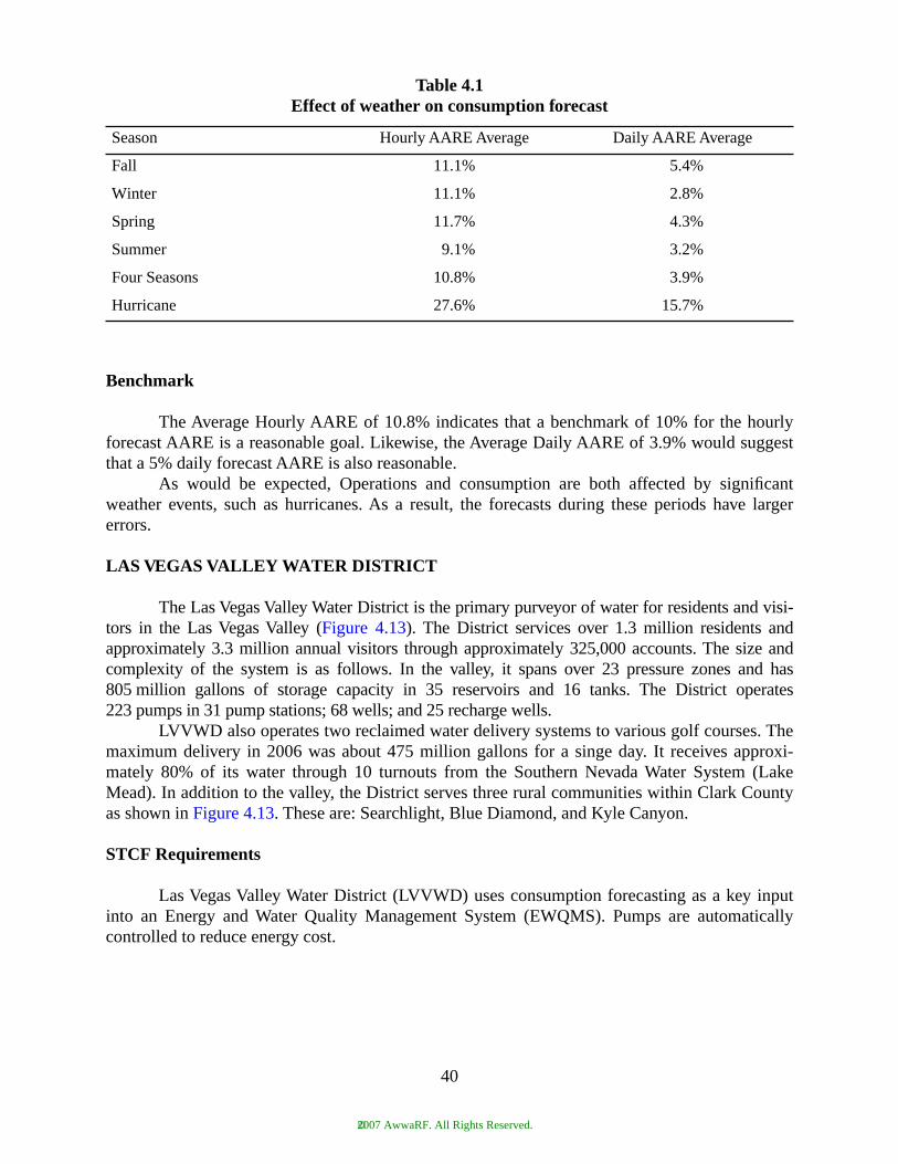
Benchmark
The Average Hourly AARE of 10.8% indicates that a benchmark of 10% for the hourlyforecast AARE is a reasonable goal. Likewise, the Average Daily AARE of 3.9% would suggestthat a 5% daily forecast AARE is also reasonable.
As would be expected, Operations and consumption are both affected by significantweather events, such as hurricanes. As a result, the forecasts during these periods have largererrors.
LAS VEGAS VALLEY WATER DISTRICT
The Las Vegas Valley Water District is the primary purveyor of water for residents and visi-tors in the Las Vegas Valley (Figure 4.13). The District services over 1.3 million residents andapproximately 3.3 million annual visitors through approximately 325,000 accounts. The size andcomplexity of the system is as follows. In the valley, it spans over 23 pressure zones and has805 million gallons of storage capacity in 35 reservoirs and 16 tanks. The District operates223 pumps in 31 pump stations; 68 wells; and 25 recharge wells.
LVVWD also operates two reclaimed water delivery systems to various golf courses. Themaximum delivery in 2006 was about 475 million gallons for a singe day. It receives approxi-mately 80% of its water through 10 turnouts from the Southern Nevada Water System (LakeMead). In addition to the valley, the District serves three rural communities within Clark Countyas shown in Figure 4.13. These are: Searchlight, Blue Diamond, and Kyle Canyon.
STCF Requirements
Las Vegas Valley Water District (LVVWD) uses consumption forecasting as a key inputinto an Energy and Water Quality Management System (EWQMS). Pumps are automaticallycontrolled to reduce energy cost.
Table 4.1Effect of weather on consumption forecast
Season Hourly AARE Average Daily AARE Average
Fall 11.1% 5.4%
Winter 11.1% 2.8%
Spring 11.7% 4.3%
Summer 9.1% 3.2%
Four Seasons 10.8% 3.9%
Hurricane 27.6% 15.7%
40
©2007 AwwaRF. All Rights Reserved.

LVVWD’s first daily consumption forecast models consisted of little more than a trendfitted to existing data. Forecasts were derived by extrapolating the trend and comparing toheuristic predictions. This process was simple, quick and reasonably accurate.
Then conditions changed. Water quality management and power purchasing programschanged the operating environment to one where knowledge of (near) future system consumptionis crucial. The ultimate goal of the Water Consumption Forecaster (WCF) is to produce the mostaccurate predictions possible. The requirement is to calculate the water consumption forecast at asystem level.
The input to the WCF consists of the following:
• Previous Consumption• Weather Observations• Water Policy Status• Day of the Month• Season of the Year
Requirements of the STCF are categorized as follows:
• Accuracy—None specified• Resolution—Daily• Distribution—System• Input Data—Manually entered by Water Resource Department staff• Human Forecaster—Water Resource Department staff• Optimization Dynamics—Data currently used only as a research tool
LVVWD, through the Southern Nevada Water Authority (SNWA), also participates in aprogram to purchase and actively resell blocks of electric power on a daily basis. Consumptionforecasting is used as a significant component in development of strategies to schedule pumpingin order to maximize the value of power to LVVWD and SNWA.
STCF Experience
The current consumption forecast system consists of seven, multivariate regression modelsand one neural network model. The neural network model inputs include daily consumption,lagged consumption, climate and other seasonal variables. A neural network for daily usage is“trained” against the list of independent variables using data beginning on January 1, 2001.
There are four general categories of variables that are regressed against daily waterconsumption. These classes include lagged usage, climate, water policy and time. Time variablesrelate water use to a particular day, month or season.
With the exception of one model, which was estimated using an automated, step-wiseregression approach, the remaining six multivariate models were estimated using expert opinionand goodness-of-fit statistics. There is no statistical rule for using seven regression models andone neural network model. A few of the regression models are similar in variable complement andcoefficient value. The actual daily forecast is generally determined by taking the average acrossthe eight models. The role of the forecast begins at the moment the average is taken to assist anexpert opinion.
41
©2007 AwwaRF. All Rights Reserved.
Lessons learned include the following:
• Weather prediction in Las Vegas is problematic, especially during summer months. Aforecast of rain does not necessarily mean rain will fall, when rain will fall, or where itwill fall. If rain falls early in the day over an area populated with golf courses, waterconsumption will likely be reduced by a greater amount than if the rain fell at theairport late in the afternoon. In other words, rain can occur in such a way as toinfluence large irrigator decisions or it will occur after those decisions have been madeand implemented. Sometimes rainfall does not occur when indicators all point to agood soaking. And, on occasion, a predicted 20% chance of rain will result in fourconsecutive days of rain. Local knowledge and a look out the window are oftenrequired to improve the forecast.
• Day of the week is an important part of the forecast. LVVWD typically sees Sundaysummer consumption drop significantly on Sunday with a large increase on Monday,often in excess of 40 MGD. Drought restrictions that limit irrigating on Sunday are notimposed after June 1st. So what causes this swing in consumption? One theory is thatturf managers “dry off” their courses to handle higher weekend traffic. They make upthe reduced water application on Monday. Other behaviors may also be influencingconsumption. The forecast models tend to over estimate Sunday consumption andunder estimate that for Monday. Judgment must be applied to adjust Sunday’s forecastdownward and Monday’s upward.
STCF Operational Performance
Three measures were used by LVVWD to judge forecast accuracy. The forecast test periodwas from July 1, 2004 through August 31, 2005. Average percentage error (APE) of the dailyforecast ranged from 0.01% to 0.39% across models. Unfortunately, APE is a somewhatmisleading error measurement. For example, given two forecasts, one 2% high the other 2% low,APE would equal 0%.
A more meaningful error measure is mean, absolute percentage error (MAPE), whichtakes the absolute value of errors before it calculates the average. Over-predictions are notcanceled out by under-predictions. MAPE varied from a low of 3.13% to a high of 3.28%. MAPEis analogous to Average Absolute Relative Error (AARE) used in this study.
A third error measure is the root mean squared error (RMSE). Since the error values aresquared, RMSE also avoids the problem of errors opposite in sign canceling each other out. Inaddition, the squaring operation penalizes large errors more than small errors. RMSE varies from12.4 million gallons to 15.2 million gallons.
SAN DIEGO WATER DEPARTMENT
Operating Background
The City of San Diego Water Department (SDWD) provides water for a population in excessof 1.4 million people, covering an area of more than 403 square miles (Figure 4.14). The San DiegoWater Distribution System consists of more than 2,890 miles of water lines, 50 water pump plants,110 pressure zones, and more than 220 million gallons (MG) of potable water storage.
42
©2007 AwwaRF. All Rights Reserved.
San Diego is an importer of water; on average, nearly 90 percent of its water supply origi-nates from northern California and the Colorado River by way of the San Diego County WaterAuthority (CWA). Imported water is treated before distribution through one of three water treat-ment plants.
The San Diego Water Distribution System supplies water to over 280,000 metered connec-tions; the City of Del Mar, the Santa Fe and San Dieguito Irrigation Districts, and the CaliforniaAmerican Water Company, which in turn serves the Cities of Coronado and Imperial Beach andportions of south San Diego. In addition, San Diego Water maintains emergency water connec-tions with neighboring water agencies.
The operating environment for San Diego is complex and will be more challenging in thefuture. The San Diego area is one of the fastest growing areas in the United States and populationincreases continue to create pressures for San Diego to do more with less. Energy prices in theCalifornia region have fluctuated greatly over the last few years and are projected to grow in thefuture. In addition, energy shortages require new strategies for demand load management andenergy conservation.
STCF Requirements
The primary purpose of the SDWD Water Demand Forecaster (WDF) is to provideconsumption data to support Operations Optimization applications. The WDF utilizes an ANN togenerate a STCF. The WDF uses historical SCADA information about water consumption for 48operating areas to predict water consumption 72 hours into the future.
Historical consumption profiles are used to develop a neural network for prediction offuture patterns. The WDF uses historical weather information to develop daily forecasts with one-hour resolution. The WDF also generates annual forecasts with daily and monthly resolution.
The WDF prepares forecasts for multiple areas in the water system and incorporateshistorical weather information and weather forecasts. The water system operating areas includethe following:
• Total system consumption• Consumption in major pressure zones (or aggregated zones)• Consumption for major water supply customers• Consumption for areas supplied by the three water treatment plants
The neural network model generates a 72-hour forecast based on the following:
• Historical flow and tank volume data (up to 7 days) including:– Hourly Average Flow history for each zone– Hourly Tank Volume history for each zone
• Historical Weather data (up to 7 days) from seven weather sites including:– Hourly Temperature – Daily Rainfall
• Weather Forecast data for seven weather sites (up to 72 hours) including:– Hourly Temperature forecast (High and Low)– Hourly Rainfall forecast
43
©2007 AwwaRF. All Rights Reserved.
WDF requirements are categorized as follows:
• Accuracy—The total daily forecast accuracy less than 5%, and the hourly forecastaccuracy less than 10%.
• Resolution—Hourly• Distribution—48 Operating Areas• Data—SCADA and NOAA weather data from the Internet• Human Forecaster—An engineer in the Optimization Group• Optimization Dynamics—Pump Schedule is developed once a day and run for the
entire day. • Weather Sensitive Consumption Parameters—air temperature and rainfall
STCF Experience
Based on a series of interviews with operations staff and water system documentation, aschematic diagram of the SDWD system was created to identify water suppliers, interconnections,water storage sites, and consumption points. The diagram was then divided into consumptionareas and equations were developed to calculate consumption. After the equations were verifiedusing real time data, historical SCADA data was used to calculate hourly consumptions over theprevious year.
Neural network models were created using historical consumption and weather data fromthe San Diego airport. The development of a prototype model involved several phases. In the firstphase, historical daily consumption for the entire system and daily weather parameters, includingmaximum temperature, minimum temperature, maximum dew point, minimum dew point, rain-fall, average wind speed, average wind direction, cloud cover, and solar index were used to predictthe daily system consumption for one day in the future. Using the statistics generated by the WDF,it was determined that average wind speed, average wind direction, cloud cover, and solar indexhad no correlation with the consumption data and they were therefore removed from the model.Furthermore, the maximum and minimum dew point parameters had no more effect on the modelthan the maximum and minimum temperature, so these values were also removed.
The second phase of development involved checking the correlation between previousconsumption and future consumption. Previous day’s consumption had a better correlation thanany of the weather parameters due, most likely, to the normally temperate weather in San Diego.Several models were tested with multiple previous days of consumption with little improvementin the model, so previous day’s consumption was retained as the best indicator.
The third phase of development involved identification of other parameters that mightimprove the prediction. Many forecasts models use a day ID (Monday = 1, Tuesday = 2 etc.) orday type (weekday = 1, weekend = 2, holiday = 3) to account for variations in consumption due tothe day of the week. For San Diego, these two parameters had little or no correlation with theconsumption pattern. However, based on interviews with operations personnel and examination ofthe historical data, it was determined that consumption tended to be highest on Monday,Wednesday, and Friday, lower on Tuesday and Thursday, even lower on Saturday, and the loweston Sunday. The historical data was manipulated to obtain an average consumption for each day ofthe week. Using the average Sunday as a reference, the percentage by which consumption foreach average day of the week exceeded that of the average Sunday was calculated and then usedto create the day codes shown in the Table 4.2.
44
©2007 AwwaRF. All Rights Reserved.
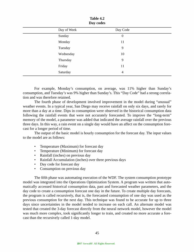
For example, Monday’s consumption, on average, was 11% higher than Sunday’sconsumption, and Tuesday’s was 9% higher than Sunday’s. This “Day Code” had a strong correla-tion and was therefore retained.
The fourth phase of development involved improvement in the model during “unusual”weather events. In a typical year, San Diego may receive rainfall on only six days, and rarely formore than a day at a time. Dips in consumption were observed in the historical consumption datafollowing the rainfall events that were not accurately forecasted. To improve the “long-term”memory of the model, a parameter was added that indicated the average rainfall over the previousthree days. In this way, a rain event on a single day would have an affect on the consumption fore-cast for a longer period of time.
The output of the basic model is hourly consumption for the forecast day. The input valuesto the model are as follows:
• Temperature (Maximum) for forecast day• Temperature (Minimum) for forecast day• Rainfall (inches) on previous day• Rainfall Accumulation (inches) over three previous days• Day code for forecast day• Consumption on previous day
The fifth phase was automating execution of the WDF. The system consumption prototypemodel was integrated into the Operations Optimization System. A program was written that auto-matically accessed historical consumption data, past and forecasted weather parameters, and theday code to create a consumption forecast one day in the future. To create multiple day forecasts,the program is called recursively, that is, the forecasted consumption of one day was used as theprevious consumption for the next day. This technique was found to be accurate for up to threedays since uncertainties in the model tended to increase on each call. An alternate model wastested that created the 3-day forecast directly from the neural network model, however the modelwas much more complex, took significantly longer to train, and created no more accurate a fore-cast than the recursively called 1-day model.
Table 4.2Day codes
Day of Week Day Code
Sunday 0
Monday 11
Tuesday 9
Wednesday 10
Thursday 9
Friday 11
Saturday 4
45
©2007 AwwaRF. All Rights Reserved.

During phase six, the basic model approach was used to train neural network models foreach consumption area (48) in the water system and integrated into the Operations OptimizationSystem.
Lessons learned included the following:
1. Missing or Invalid Weather Data—Occasionally there are gaps in the historicalweather data record or weather forecast that is not available. Care must be taken to usereliable sources of weather data, preferably a source that provides “corrected” datarather than “raw” data.
2. Missing or Invalid Historical Consumption Data—Similar to missing weather data,missing or invalid consumption data must be corrected to enable an accurate forecast.
3. Sensitivity to System Maintenance—Field maintenance, which affects water systemtopology, can affect consumption in one or more operating areas.
4. Sensitivity to Weather Events—Neural Networks are very good at “interpolation”, butnot at “extrapolation.” In the case of San Diego, extended periods of rainfall can affectthe accuracy of the forecasts.
5. Re-training of Neural Network—For small systems with limited operating areas thatchange infrequently, manually re-training the neural networks is acceptable. Auto-matic re-training increases development costs. However, with more complex systems,maintenance costs are reduced by automatic retraining.
STCF Operational Performance
Data from one operating area was collected for twenty-eight days, seven days from eachseason, for analysis. Figures 4.15 to 4.22 are graphs of the hourly and daily consumptions for eachseason.
Extreme Weather
San Diego’s climate is very dry. Total precipitation for 2004 was 15.3 inches. Winter of2005 was unusually wet, with 4.8 inches in January and 5.8 inches in February. Over the period ofFebruary 18, 2005 through February 24, 2005, a total of 4.17 inches of rain fell; 2.14 inches onFebruary 22 alone. The heavy rains resulted in flooding and mud slides. Figure 4.23 illustrates thehourly accuracy of the forecast during a week with heavy rains in February 2005. Note the largeerrors in the forecast between hours 97 and 121 as the result of heavy rainfall. Figure 4.24 illus-trates the daily forecast for the same week. The daily forecast was not significantly impairedduring this week.
Error Analysis
The ANN Forecast closely followed consumption. Table 4.3 is a summary of the AverageAbsolute Relative Errors (AARE).
46
©2007 AwwaRF. All Rights Reserved.
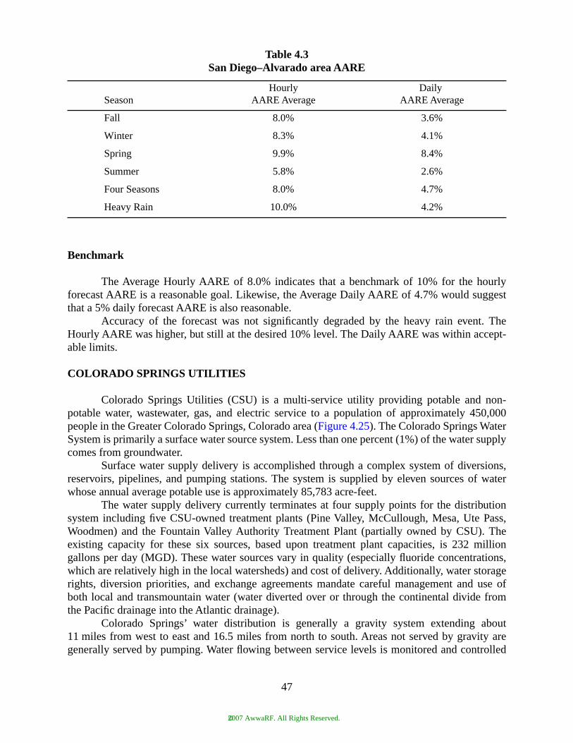
Benchmark
The Average Hourly AARE of 8.0% indicates that a benchmark of 10% for the hourlyforecast AARE is a reasonable goal. Likewise, the Average Daily AARE of 4.7% would suggestthat a 5% daily forecast AARE is also reasonable.
Accuracy of the forecast was not significantly degraded by the heavy rain event. TheHourly AARE was higher, but still at the desired 10% level. The Daily AARE was within accept-able limits.
COLORADO SPRINGS UTILITIES
Colorado Springs Utilities (CSU) is a multi-service utility providing potable and non-potable water, wastewater, gas, and electric service to a population of approximately 450,000people in the Greater Colorado Springs, Colorado area (Figure 4.25). The Colorado Springs WaterSystem is primarily a surface water source system. Less than one percent (1%) of the water supplycomes from groundwater.
Surface water supply delivery is accomplished through a complex system of diversions,reservoirs, pipelines, and pumping stations. The system is supplied by eleven sources of waterwhose annual average potable use is approximately 85,783 acre-feet.
The water supply delivery currently terminates at four supply points for the distributionsystem including five CSU-owned treatment plants (Pine Valley, McCullough, Mesa, Ute Pass,Woodmen) and the Fountain Valley Authority Treatment Plant (partially owned by CSU). Theexisting capacity for these six sources, based upon treatment plant capacities, is 232 milliongallons per day (MGD). These water sources vary in quality (especially fluoride concentrations,which are relatively high in the local watersheds) and cost of delivery. Additionally, water storagerights, diversion priorities, and exchange agreements mandate careful management and use ofboth local and transmountain water (water diverted over or through the continental divide fromthe Pacific drainage into the Atlantic drainage).
Colorado Springs’ water distribution is generally a gravity system extending about11 miles from west to east and 16.5 miles from north to south. Areas not served by gravity aregenerally served by pumping. Water flowing between service levels is monitored and controlled
Table 4.3San Diego–Alvarado area AARE
SeasonHourly
AARE AverageDaily
AARE Average
Fall 8.0% 3.6%
Winter 8.3% 4.1%
Spring 9.9% 8.4%
Summer 5.8% 2.6%
Four Seasons 8.0% 4.7%
Heavy Rain 10.0% 4.2%
47
©2007 AwwaRF. All Rights Reserved.
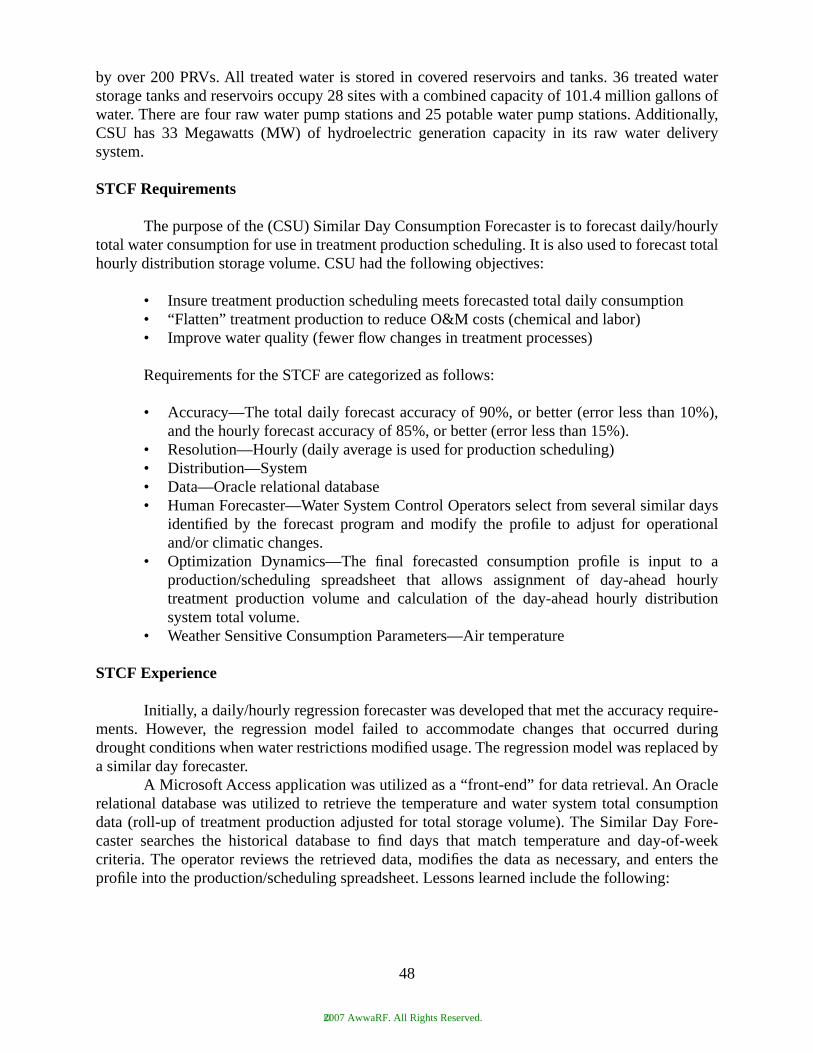
by over 200 PRVs. All treated water is stored in covered reservoirs and tanks. 36 treated waterstorage tanks and reservoirs occupy 28 sites with a combined capacity of 101.4 million gallons ofwater. There are four raw water pump stations and 25 potable water pump stations. Additionally,CSU has 33 Megawatts (MW) of hydroelectric generation capacity in its raw water deliverysystem.
STCF Requirements
The purpose of the (CSU) Similar Day Consumption Forecaster is to forecast daily/hourlytotal water consumption for use in treatment production scheduling. It is also used to forecast totalhourly distribution storage volume. CSU had the following objectives:
• Insure treatment production scheduling meets forecasted total daily consumption• “Flatten” treatment production to reduce O&M costs (chemical and labor) • Improve water quality (fewer flow changes in treatment processes)
Requirements for the STCF are categorized as follows:
• Accuracy—The total daily forecast accuracy of 90%, or better (error less than 10%),and the hourly forecast accuracy of 85%, or better (error less than 15%).
• Resolution—Hourly (daily average is used for production scheduling)• Distribution—System• Data—Oracle relational database• Human Forecaster—Water System Control Operators select from several similar days
identified by the forecast program and modify the profile to adjust for operationaland/or climatic changes.
• Optimization Dynamics—The final forecasted consumption profile is input to aproduction/scheduling spreadsheet that allows assignment of day-ahead hourlytreatment production volume and calculation of the day-ahead hourly distributionsystem total volume.
• Weather Sensitive Consumption Parameters—Air temperature
STCF Experience
Initially, a daily/hourly regression forecaster was developed that met the accuracy require-ments. However, the regression model failed to accommodate changes that occurred duringdrought conditions when water restrictions modified usage. The regression model was replaced bya similar day forecaster.
A Microsoft Access application was utilized as a “front-end” for data retrieval. An Oraclerelational database was utilized to retrieve the temperature and water system total consumptiondata (roll-up of treatment production adjusted for total storage volume). The Similar Day Fore-caster searches the historical database to find days that match temperature and day-of-weekcriteria. The operator reviews the retrieved data, modifies the data as necessary, and enters theprofile into the production/scheduling spreadsheet. Lessons learned include the following:
48
©2007 AwwaRF. All Rights Reserved.

• Unusual conditions, such as a drought, can modify usage patterns and have a negativeimpact on regression forecast models
• Data quality is important to avoid significant errors in consumption profiles that couldcause incorrect production scheduling decisions and storage operation errors
The advantages of the Similar Day Forecaster include the following:
• Low Cost—Requires only a database application and readily available data• Ease of Use—Profiles are easy to select and modify• Takes advantage of operator experience and judgment
The disadvantages of the Similar Day Forecaster are:
• Inconsistency—Errors are introduced since different operators use the system throughthe course of the day and week
• Time consuming—Although easy to use, time is required to review and update theconsumption profiles
STCF Operational Performance
The original objectives and requirements for the STCF were met with the Similar DayForecaster. A real time database application has been added to introduce near-real time data toprovide continuous feedback of model accuracy. In addition, CSU is considering other weathersensitive factors beyond temperature for selection of the “similar days.”
The next step for CSU is to investigate other technologies, such as neural networks, tosupport or replace the Similar Day Forecaster.
Data from the system were collected for twenty-eight days, seven days from each season,for analysis. Figures 4.26 to 4.33 are graphs of the hourly and daily forecasts versus consumptionfor each season.
Error Analysis
The Similar Day Forecast closely followed consumption. Table 4.4 is a summary of theAverage Absolute Relative Errors (AARE).
Benchmark
The Average Hourly AARE of 8.0% indicates that a benchmark of 10% for the hourlyforecast AARE is a reasonable goal. Likewise, the Average Daily AARE of 4.1% would suggestthat a 5% daily forecast AARE is also reasonable.
SUMMARY
Table 4.5 provides a summary of the analysis of STCF systems at the four utilities. Theyreflect the results of operational STCF systems during four seasons of one year. Analysis of the
49
©2007 AwwaRF. All Rights Reserved.
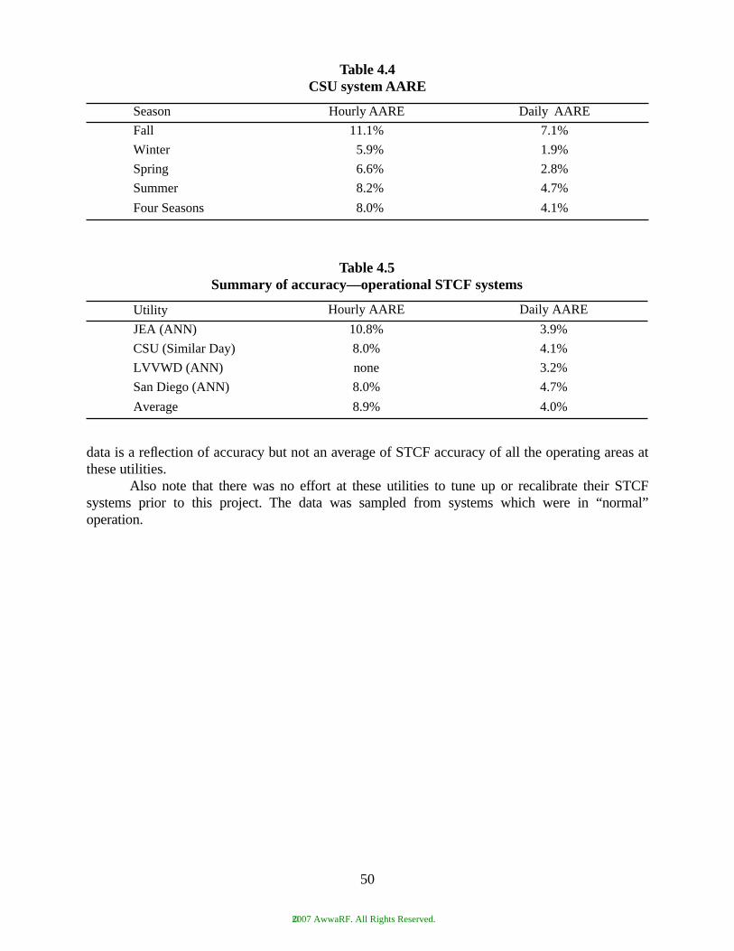
data is a reflection of accuracy but not an average of STCF accuracy of all the operating areas atthese utilities.
Also note that there was no effort at these utilities to tune up or recalibrate their STCFsystems prior to this project. The data was sampled from systems which were in “normal”operation.
Table 4.4CSU system AARE
Season Hourly AARE Daily AARE
Fall 11.1% 7.1%
Winter 5.9% 1.9%
Spring 6.6% 2.8%
Summer 8.2% 4.7%
Four Seasons 8.0% 4.1%
Table 4.5Summary of accuracy—operational STCF systems
Utility Hourly AARE Daily AARE
JEA (ANN) 10.8% 3.9%
CSU (Similar Day) 8.0% 4.1%
LVVWD (ANN) none 3.2%
San Diego (ANN) 8.0% 4.7%
Average 8.9% 4.0%
50
©2007 AwwaRF. All Rights Reserved.
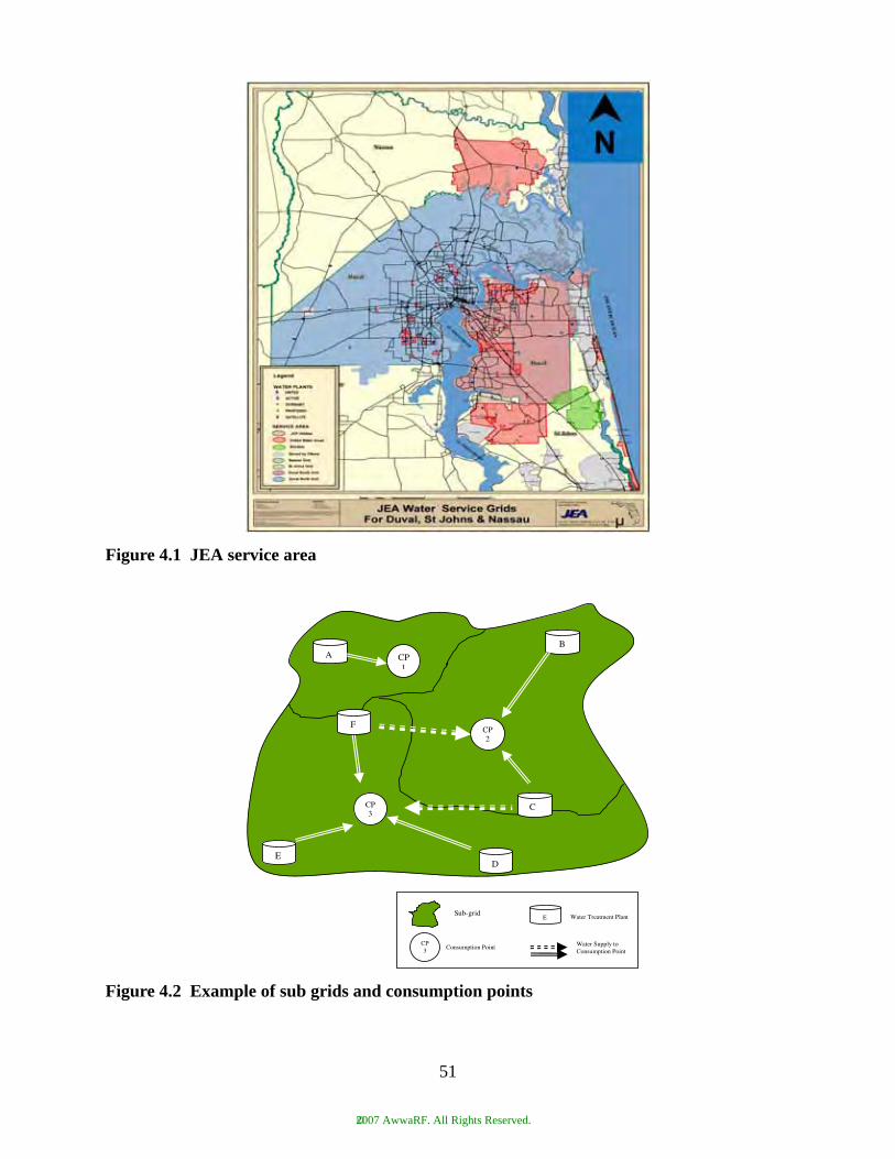
51
Figure 4.1 JEA service area
Figure 4.2 Example of sub grids and consumption points
AB
ED
CP3
CP 2
CP 1
F
C
E
CP3
Sub-grid
Water Supply to Consumption Point
Consumption Point
Water Treatment Plant
©2007 AwwaRF. All Rights Reserved.
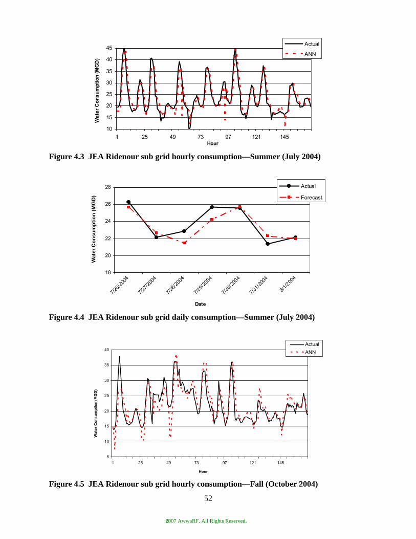
52
Figure 4.3 JEA Ridenour sub grid hourly consumption—Summer (July 2004)
Figure 4.4 JEA Ridenour sub grid daily consumption—Summer (July 2004)
Figure 4.5 JEA Ridenour sub grid hourly consumption—Fall (October 2004)
10
15
20
25
30
35
40
45
1 25 49 73 97 121 145Hour
)D
GM(
noit
pm
us
no
C ret
aW
Actual
ANN
18
20
22
24
26
28
/7/62
4002
7/72/
40024002/82/7 /7
/92
40024002/03/7 /7
/13
40024002/1/8
Date
)D
GM(
noit
pm
usn
oC reta
W
Actual
Forecast
5
10
15
20
25
30
35
40
1 25 49 73 97 121 145
Hour
)D
GM(
noit
pm
us
no
C ret
aW
Actual
ANN
©2007 AwwaRF. All Rights Reserved.
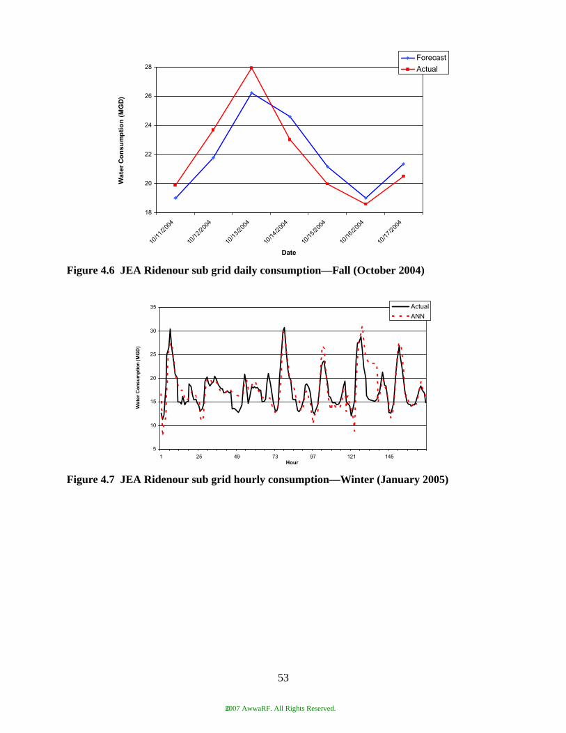
Figure 4.6 JEA Ridenour sub grid daily consumption—Fall (October 2004)
Figure 4.7 JEA Ridenour sub grid hourly consumption—Winter (January 2005)
18
20
22
24
26
28
4002/11/01
4002/21/01
4002/31/011/014/2
040
/0151/2
040
01/
4002/61
4002/71/01
Date
)D
GM(
noit
pm
usn
oC reta
W
Forecast
Actual
5
10
15
20
25
30
35
1 25 49 73 97 121 145Hour
)D
GM(
noit
pm
us
no
C ret
aW
Actual
ANN
53
©2007 AwwaRF. All Rights Reserved.
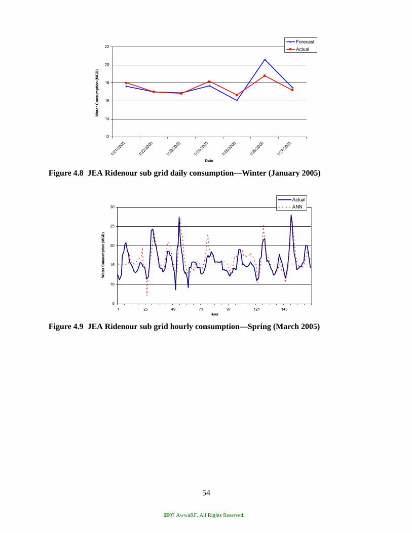
Figure 4.8 JEA Ridenour sub grid daily consumption—Winter (January 2005)
Figure 4.9 JEA Ridenour sub grid hourly consumption—Spring (March 2005)
12
14
16
18
20
22
5002/12/1 /12
002/2
5
1/32/2
005 5002/42/1
002/52/1
5
1/62/2
005
72/1/
0205
Date
)D
GM(
noit
pm
us
no
C ret
aW
Forecast
Actual
5
10
15
20
25
30
1 25 49 73 97 121 145Hour
)D
GM(
noit
pm
us
no
C ret
aW
Actual
ANN
54
©2007 AwwaRF. All Rights Reserved.
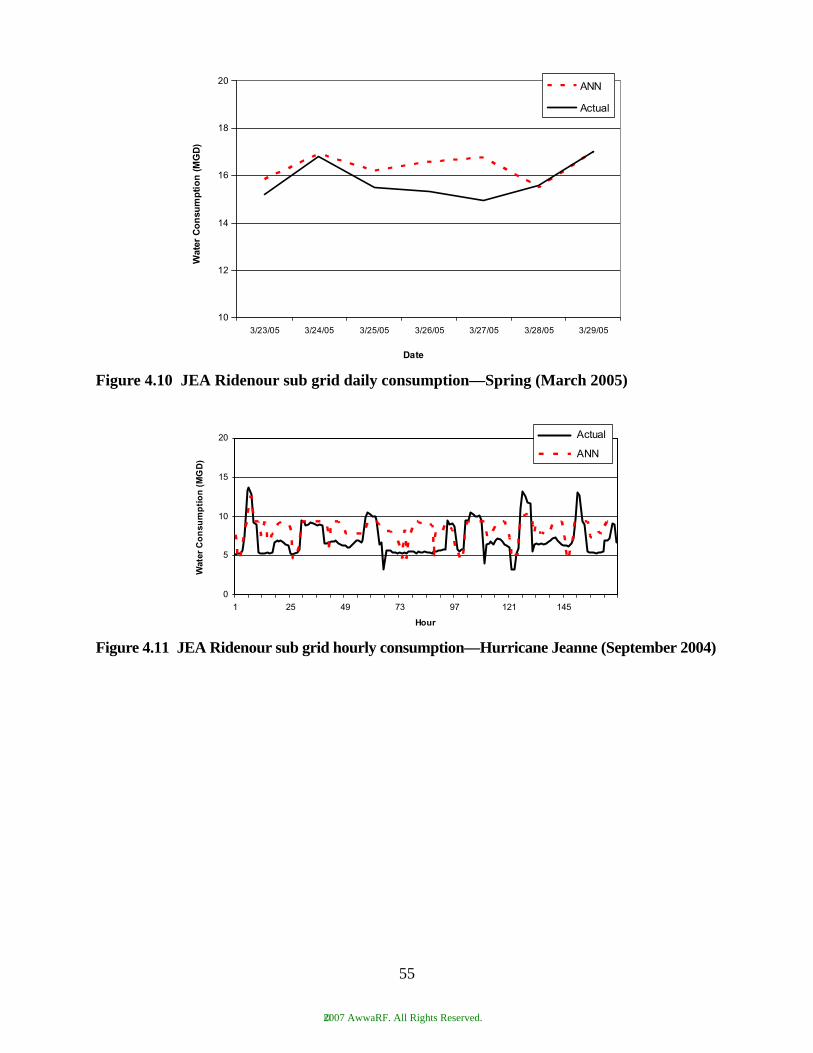
Figure 4.10 JEA Ridenour sub grid daily consumption—Spring (March 2005)
Figure 4.11 JEA Ridenour sub grid hourly consumption—Hurricane Jeanne (September 2004)
10
12
14
16
18
20
3/23/05 3/24/05 3/25/05 3/26/05 3/27/05 3/28/05 3/29/05
Date
)D
GM(
noit
pm
usn
oC reta
W
ANN
Actual
0
5
10
15
20
1 25 49 73 97 121 145
Hour
)D
GM(
noit
pm
usn
oC reta
W
Actual
ANN
55
©2007 AwwaRF. All Rights Reserved.
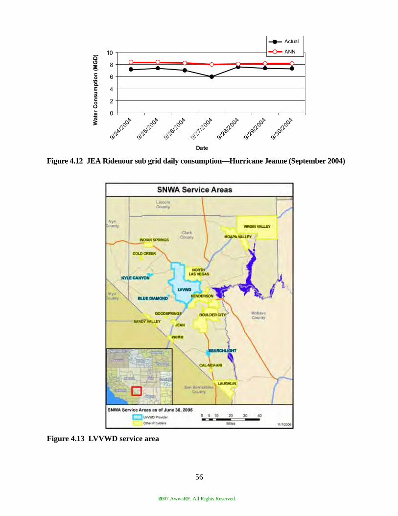
Figure 4.12 JEA Ridenour sub grid daily consumption—Hurricane Jeanne (September 2004)
Figure 4.13 LVVWD service area
0
2
4
6
8
10
4002/42/9 9/52
2/0
40
/92
4002/6 /72/9
2004 002/82/9
4
9/92
2/0
40 4002/03/9
Date
)D
GM(
noit
pm
usn
oC reta
W
Actual
ANN
56
©2007 AwwaRF. All Rights Reserved.
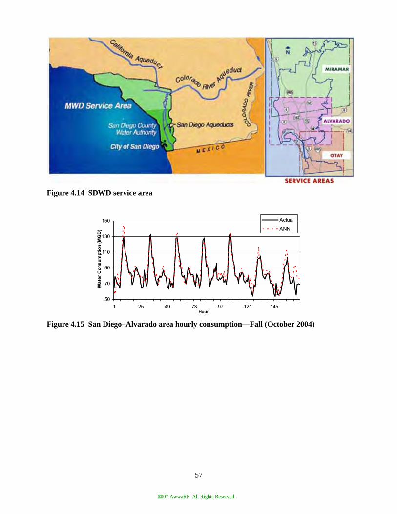
Figure 4.14 SDWD service area
Figure 4.15 San Diego–Alvarado area hourly consumption—Fall (October 2004)
50
70
90
110
130
150
1 25 49 73 97 121 145Hour
)D
GM(
noit
pm
us
no
C ret
aW
Actual
ANN
57
©2007 AwwaRF. All Rights Reserved.
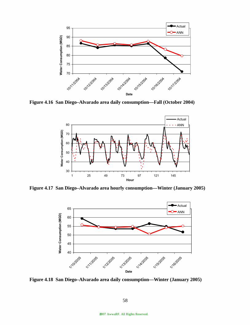
Figure 4.16 San Diego–Alvarado area daily consumption—Fall (October 2004)
Figure 4.17 San Diego–Alvarado area hourly consumption—Winter (January 2005)
Figure 4.18 San Diego–Alvarado area daily consumption—Winter (January 2005)
70
75
80
85
90
95
01/ 11
/02
40
1/021/2
400
01/
002/31
4
01/ 41
/02
40
1/051/2
400
01/
002/61
4
01/ 71
/02
40
Date
)D
GM(
noit
pm
us
no
C ret
aW
Actual
ANN
30
40
50
60
70
80
1 25 49 73 97 121 145Hour
)D
GM(
noit
pm
us
no
C ret
aW
Actual
ANN
40
45
50
55
60
65
/101/
0205
/111
2/0
50
/121/
0250
/131/
0250
1/14
2/0
50
/151
2/0
50
/161/
5002
Date
)D
GM(
noit
pm
us
no
C ret
aW
Actual
ANN
58
©2007 AwwaRF. All Rights Reserved.
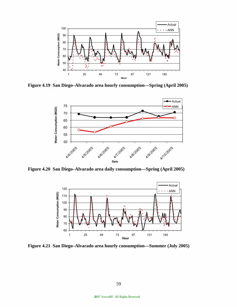
Figure 4.19 San Diego–Alvarado area hourly consumption—Spring (April 2005)
Figure 4.20 San Diego–Alvarado area daily consumption—Spring (April 2005)
Figure 4.21 San Diego–Alvarado area hourly consumption—Summer (July 2005)
40
50
60
70
80
90
100
1 25 49 73 97 121 145Hour
)D
GM(
noit
pm
usn
oC reta
W
Actual
ANN
50
55
60
65
70
75
5002/4/42/5/4
050
4/602/05
4/702/05
4/802/05
2/9/4
050
/01/4
2500
Date
)D
GM(
noit
pm
us
no
C ret
aW
Actual
ANN
60
70
80
90
100
110
120
1 25 49 73 97 121 145Hour
)D
GM(
noit
pm
us
no
C ret
aW
Actual
ANN
59
©2007 AwwaRF. All Rights Reserved.
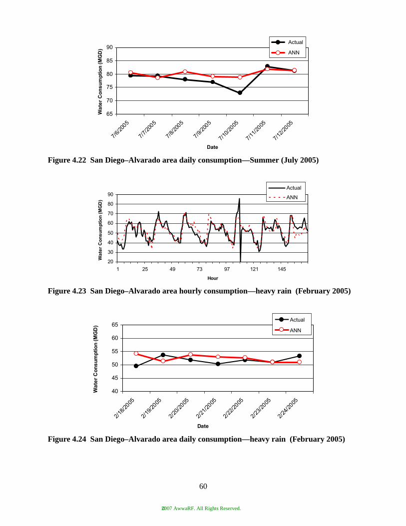
Figure 4.22 San Diego–Alvarado area daily consumption—Summer (July 2005)
Figure 4.23 San Diego–Alvarado area hourly consumption—heavy rain (February 2005)
Figure 4.24 San Diego–Alvarado area daily consumption—heavy rain (February 2005)
65
70
75
80
85
90
/76/
0025
/77
2/005
78//
50029/7/
5002/71
/02
500 002/11/7
5 5002/21/7
Date
)D
GM(
noit
pm
us
no
C ret
aW
Actual
ANN
20
30
40
50
60
70
80
90
1 25 49 73 97 121 145
Hour
)D
GM(
noit
pm
us
no
C ret
aW
Actual
ANN
40
45
50
55
60
65
/21
/82
5005002/91/2
002/02/2
5 002/12/2
5 5002/22/2
5002/32/2 2/42/
0250
Date
)D
GM(
noit
pm
us
no
C ret
aW
Actual
ANN
60
©2007 AwwaRF. All Rights Reserved.
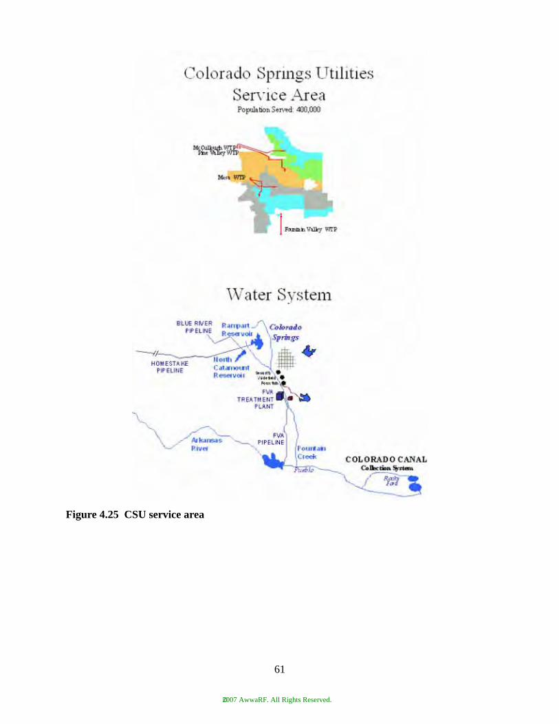
Figure 4.25 CSU service area
61
©2007 AwwaRF. All Rights Reserved.
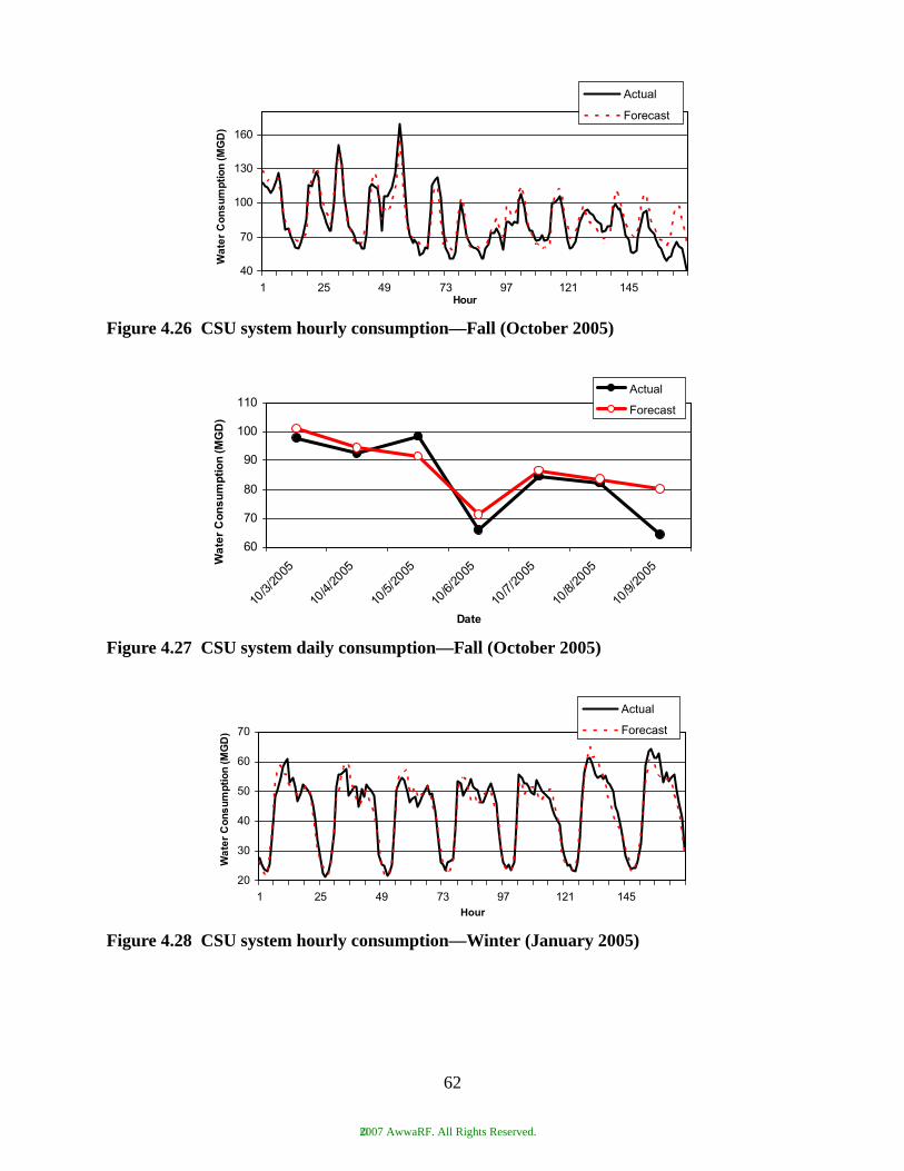
Figure 4.26 CSU system hourly consumption—Fall (October 2005)
Figure 4.27 CSU system daily consumption—Fall (October 2005)
Figure 4.28 CSU system hourly consumption—Winter (January 2005)
40
70
100
130
160
1 25 49 73 97 121 145Hour
)D
GM(
noit
pm
us
no
C ret
aW
Actual
Forecast
60
70
80
90
100
110
1/03
2/0
504/01/
5002
1/05
5002/10
6/ /0205
1/07/
0250
108/ /
0250
1/09
2/0
50
Date
)D
GM(
noit
pm
us
no
C ret
aW
Actual
Forecast
20
30
40
50
60
70
1 25 49 73 97 121 145Hour
)D
GM(
noit
pm
us
no
C ret
aW
Actual
Forecast
62
©2007 AwwaRF. All Rights Reserved.
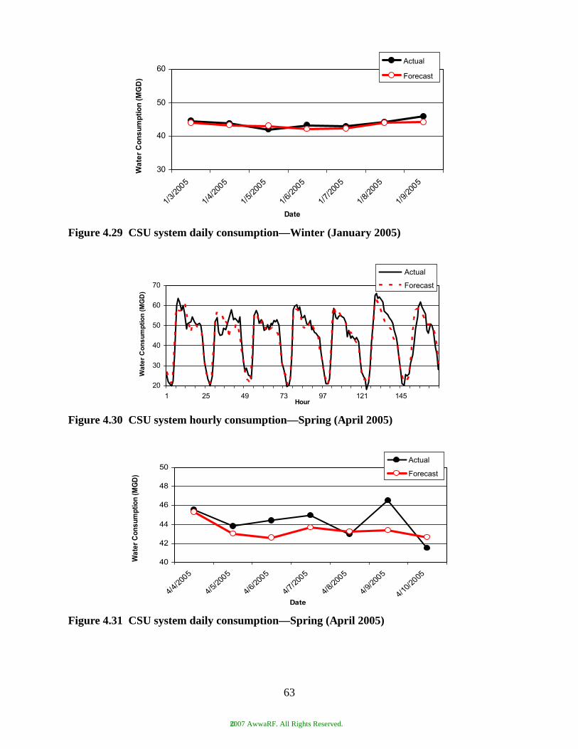
Figure 4.29 CSU system daily consumption—Winter (January 2005)
Figure 4.30 CSU system hourly consumption—Spring (April 2005)
Figure 4.31 CSU system daily consumption—Spring (April 2005)
30
40
50
60
3/1/
0205
/1/42
005
/1/52
005
/1
002/6
5
/1
002/7
5
/1
002/8
5
/1
5002/9
Date
)D
GM(
noit
pm
us
no
C ret
aW
Actual
Forecast
20
30
40
50
60
70
1 25 49 73 97 121 145Hour
)D
GM(
noit
pm
us
no
C ret
aW
Actual
Forecast
40
42
44
46
48
50
44//
0205
45//
0205
4/
002/6
5
4/
002/7
5
4/
002/8
5
4//92
005
4/01/
0250
Date
)D
GM( noitp
musnoC reta
W
Actual
Forecast
63
©2007 AwwaRF. All Rights Reserved.
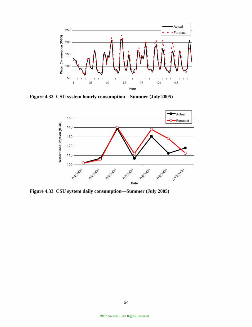
Figure 4.32 CSU system hourly consumption—Summer (July 2005)
Figure 4.33 CSU system daily consumption—Summer (July 2005)
50
100
150
200
250
1 25 49 73 97 121 145
Hour
)D
GM(
noit
pm
us
no
C ret
aW
Actual
Forecast
100
110
120
130
140
150
4/7/
0205
/7
5002/5 /7
002/6
5 5002/7/7 /7
002/8
5
/7/9
0205 5002/01/7
Date
)D
GM(
noit
pm
us
no
C ret
aW
Actual
Forecast
64
©2007 AwwaRF. All Rights Reserved.
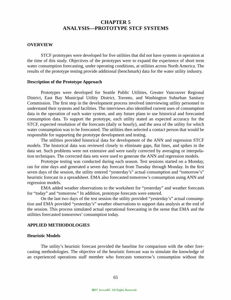
CHAPTER 5ANALYSIS—PROTOTYPE STCF SYSTEMS
OVERVIEW
STCF prototypes were developed for five utilities that did not have systems in operation atthe time of this study. Objectives of the prototypes were to expand the experience of short termwater consumption forecasting, under operating conditions, at utilities across North America. Theresults of the prototype testing provide additional (benchmark) data for the water utility industry.
Description of the Prototype Approach
Prototypes were developed for Seattle Public Utilities, Greater Vancouver RegionalDistrict, East Bay Municipal Utility District, Toronto, and Washington Suburban SanitaryCommission. The first step in the development process involved interviewing utility personnel tounderstand their systems and facilities. The interviews also identified current uses of consumptiondata in the operation of each water system, and any future plans to use historical and forecastedconsumption data. To support the prototype, each utility stated an expected accuracy for theSTCF, expected resolution of the forecasts (daily or hourly), and the area of the utility for whichwater consumption was to be forecasted. The utilities then selected a contact person that would beresponsible for supporting the prototype development and testing.
The utilities provided historical data for development of the ANN and regression STCFmodels. The historical data was reviewed closely to eliminate gaps, flat lines, and spikes in thedata set. Such problems were not extensive and were easily corrected by averaging or interpola-tion techniques. The corrected data sets were used to generate the ANN and regression models.
Prototype testing was conducted during each season. Test sessions started on a Monday,ran for nine days and generated a seven day forecast from Tuesday through Monday. In the firstseven days of the session, the utility entered “yesterday’s” actual consumption and “tomorrow’s”heuristic forecast in a spreadsheet. EMA also forecasted tomorrow’s consumption using ANN andregression models.
EMA added weather observations to the worksheet for “yesterday” and weather forecastsfor “today” and “tomorrow.” In addition, prototype forecasts were entered.
On the last two days of the test session the utility provided “yesterday’s” actual consump-tion and EMA provided “yesterday’s” weather observations to support data analysis at the end ofthe session. This process simulated actual operational forecasting in the sense that EMA and theutilities forecasted tomorrows’ consumption today.
APPLIED METHODOLOGIES
Heuristic Models
The utility’s heuristic forecast provided the baseline for comparison with the other fore-casting methodologies. The objective of the heuristic forecast was to simulate the knowledge ofan experienced operations staff member who forecasts tomorrow’s consumption without the
65
©2007 AwwaRF. All Rights Reserved.

benefit of forecasting software. To maintain consistency among the utilities, the following groundrules were established:
• Utility staff developed a heuristic forecast• Utility did not use data from pre-existing forecast models• Utility was allowed to use trends/past consumption data to support the forecast• EMA would not be influenced by heuristic forecast results• Worksheets would be write-protected to avoid “accidental” changes in data
SPU used a combination of existing forecasting tools and trends of historical data to createtheir heuristic forecasts.
The GVRD heuristic model was based on the “Last Four Day” method. To forecast for aMonday, for example, the hourly consumption, daily consumption and maximum temperature forthe previous four Mondays, and the forecasted maximum temperature for the Monday to be fore-casted were used to forecast the hourly and daily consumption for the “Fifth Day.” The basic stepsof the GVRD heuristic model were as follows:
1. An average daily consumption was calculated using the daily consumption from theprevious four days.
2. An adjustment factor was calculated based on a ratio of the forecasted next day maxi-mum temperature and the average maximum temperatures on the previous four days.
3. The adjustment factor was applied to the average daily consumption from Step 1 toobtain the forecasted daily consumption.
4. For each previous day, the hourly consumption for each hour was divided by the dailyconsumption for the day to create a “normalized” hourly profile.
5. The “normalized” hourly profiles were averaged together and the resulting profile wasapplied to the forecasted daily consumption to obtain the forecasted hourly consump-tion profile.
The EBMUD heuristic model consisted of estimating daily consumption and applying anhourly consumption pattern based on the time of the year, consumption ranges and day of theweek. The basic steps of the EBMUD heuristic model were:
1. Daily Consumption—Daily consumption one month prior to the test period was plot-ted. The trend was used to identify how consumption varied with day of the week. Theprevious day’s consumption was used as a starting point for prediction of the next dayconsumption. Based on the next day weather forecast and day of the week, consump-tion was added to or subtracted from the starting point consumption to develop thedaily consumption estimate.
2. Hourly Consumption—the development of the diurnal consumption pattern was basedon the same twenty-nine months of consumption data provided to EMA for develop-ment of the ANN model. Patterns were organized by month, range of daily consump-tion and weekend/weekday. The appropriate hourly consumption pattern was appliedto the daily consumption estimate to determine hourly consumption estimate.
66
©2007 AwwaRF. All Rights Reserved.

The Toronto heuristic model involved estimation of the daily forecast and the applicationof hourly consumption pattern on a similar day. The following steps were used:
1. Daily consumption from a year ago was used to determine a seasonal trend.2. Daily consumption from a week ago provided a more current daily forecast.3. Historical and forecast weather data were used to adjust the daily forecast.4. The adjusted daily forecast and weather data were used to identify a similar day.5. The hourly profile on the similar day and the hourly profile from “yesterday” were
applied to the daily forecast to create the hourly forecast.
The WSSC heuristic model used day-of-the-week considerations, historical data andweather information to predict the hourly consumption for future days. The forecasted dailyconsumption was the average of the forecasted hourly values. Two cases were considered, asfollows:
• Weekday—The most recent weekday figures were used as a template and weremultiplied by a factor to take into account weather conditions and daily consumptiontrends. For example, if the prediction day is expected to be warmer or dryer, the factormight be something like 1.03. The factor was also increased if daily trends indicate anincrease in consumption due to lack of rain.
• Weekend—The hourly figures from previous Saturdays or Sundays (which had similarweather conditions) were multiplied by a similar factor to arrive at predicted hourlyconsumption figures.
Artificial Neural Network (ANN) Models
For each utility, EMA created an Artificial Neural Network (ANN) Model. An ANN modelis a mathematical model inspired by biological nervous systems. Refer to Chapter 2 for a descrip-tion of the ANN Model.
The Gensym Corporation NeurOn-Line tool was used to develop the ANN models foreach utility using the following steps:
1. Acquired historical consumption data from the utility2. Identified and corrected missing/bad data in data set3. Acquired, reviewed and corrected weather data from NOAA4. Added temporal factors (Day of Week, Day Type, etc.) to data set5. Trained several prototype models to determine best model
All of the models used previous day’s consumption and tomorrow’s weather forecast topredict tomorrow’s consumption forecast.
Once the best model was identified, the same ANN model was used throughout the test forEBMUD, SPU, and GVRD. To determine the impact of retraining the ANN model, the Torontoand WSSC ANN models were retrained prior to the winter test period.
67
©2007 AwwaRF. All Rights Reserved.

Regression Model
In addition to the ANN model, a regression model was created by EMA for Toronto andWSSC. The regression model first estimated the daily consumption and then estimated how thatconsumption was distributed across the day. The algorithms used the previous six weeks of histor-ical data in each calculation.
The daily total consumption for each day from the previous six weeks was arranged inrows and columns with the columns corresponding to days of the week (Sunday, Monday, etc.).Each column was calculated to come up with an average consumption for each day of the week.Then the last known daily consumption was multiplied by the ratio of average consumption forthe day of the estimate and divided by the average consumption of the last known daily value.
For example, to estimate the consumption for Tuesday:
• The last known daily consumption rate was 1292 ML/day for a Sunday.• The average consumption was 1430 ML/day for a Sunday and 1536 ML/day for a
Tuesday.• The estimated consumption for Tuesday is (1292)*(1536/1430) = 1,388 ML/day
The hourly distribution of the daily consumption was calculated based on historical datafrom the previous six weeks. Data from the six previous same days of the week were arranged incolumns and rows where each column represents an hour of the day. Data was normalized bydividing each hour’s consumption by the daily total. The six normalized values for each hour wereaveraged to calculate a normalized daily distribution. The forecasted daily consumption wasapplied to this normalized profile to create the hourly forecast.
Using the example above:
• The normalized value for 3:00 AM was 0.66 and the normalized value for 10:00 PM
was 1.25. (Values were calculated for each hour of the day)• The estimated consumption at 3:00 AM was 1,388*0.66 = 916 ML/day• The estimated consumption at 10:00 PM was 1,388*1.25 = 1,735 ML/day• This calculation was repeated for each hour to produce the hourly forecast
Measurement Criteria
The primary measure of performance is the Absolute Relative Error (ARE) calculated asfollows:
ARE (%) = 100 × | (Forecast – Actual) / Actual |
For example, assuming a forecast value of 90 and an actual value of 100 the ARE would be 10%.Average Absolute Relative Error (AARE) is calculated by taking the average of the ARE
values. The Hourly AARE is the average of the Hourly ARE values. The Daily AARE is theaverage of Daily AARE values.
68
©2007 AwwaRF. All Rights Reserved.

SEATTLE PUBLIC UTILITIES
Description of Service Area and Facilities
Seattle Public Utilities (SPU) provides water supply and wastewater collection services tothe City of Seattle and King County. Seattle Public Utilities provides direct retail water service toabout 630,000 people in the City of Seattle, parts of Shoreline and small areas just south of thecity limits. Figure 5.1 shows an overview of the Seattle Water System.
Current Uses for Calculated and Forecasted Consumption Information
SPU currently uses a number of sophisticated modeling tools to forecast consumption tosupport planning for future development.
Future Uses for Forecasted Consumption Information
SPU plans to use a STCF to forecast daily and hourly consumption as a component of anOperations Optimization System for water supply, treatment plant, and pump scheduling.
Formal Definition of STCF Requirements
A daily forecast will be developed for the entire system. The Average Absolute RelativeError (AARE) is expected to be less than 10% for the daily forecast. The daily forecast isexpected to be sensitive to variations in air temperature and rainfall.
Test Results
The results of daily consumption forecasting for the four seasons are shown in Figures 5.2to 5.5.
Summary of Results
Table 5.1 is a summary of the Daily AARE values.
GREATER VANCOUVER REGIONAL DISTRICT
Description of Service Area and Facilities
The Greater Vancouver Regional District (GVRD) provides water, solid waste, sewage,and drainage services to 21 member municipalities and one electoral area with a total servicepopulation of 2 million. Surface water is supplied from three protected sources. The systemconsists of over 500 km of large diameter welded steel transmission mains and 22 storage reser-voirs to buffer daily demand variations. Figure 5.6 shows an overview of the GVRD service area.
69
©2007 AwwaRF. All Rights Reserved.
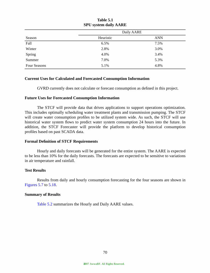
Current Uses for Calculated and Forecasted Consumption Information
GVRD currently does not calculate or forecast consumption as defined in this project.
Future Uses for Forecasted Consumption Information
The STCF will provide data that drives applications to support operations optimization.This includes optimally scheduling water treatment plants and transmission pumping. The STCFwill create water consumption profiles to be utilized system wide. As such, the STCF will usehistorical water system flows to predict water system consumption 24 hours into the future. Inaddition, the STCF Forecaster will provide the platform to develop historical consumptionprofiles based on past SCADA data.
Formal Definition of STCF Requirements
Hourly and daily forecasts will be generated for the entire system. The AARE is expectedto be less than 10% for the daily forecasts. The forecasts are expected to be sensitive to variationsin air temperature and rainfall.
Test Results
Results from daily and hourly consumption forecasting for the four seasons are shown inFigures 5.7 to 5.18.
Summary of Results
Table 5.2 summarizes the Hourly and Daily AARE values.
Table 5.1SPU system daily AARE
Season
Daily AARE
Heuristic ANN
Fall 6.5% 7.5%
Winter 2.8% 3.0%
Spring 4.0% 3.4%
Summer 7.0% 5.3%
Four Seasons 5.1% 4.8%
70
©2007 AwwaRF. All Rights Reserved.
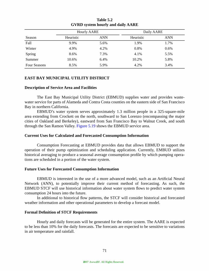
EAST BAY MUNICIPAL UTILITY DISTRICT
Description of Service Area and Facilities
The East Bay Municipal Utility District (EBMUD) supplies water and provides waste-water service for parts of Alameda and Contra Costa counties on the eastern side of San FranciscoBay in northern California.
EBMUD’s water system serves approximately 1.3 million people in a 325-square-milearea extending from Crockett on the north, southward to San Lorenzo (encompassing the majorcities of Oakland and Berkeley), eastward from San Francisco Bay to Walnut Creek, and souththrough the San Ramon Valley. Figure 5.19 shows the EBMUD service area.
Current Uses for Calculated and Forecasted Consumption Information
Consumption Forecasting at EBMUD provides data that allows EBMUD to support theoperation of their pump optimization and scheduling application. Currently, EMBUD utilizeshistorical averaging to produce a seasonal average consumption profile by which pumping opera-tions are scheduled in a portion of the water system.
Future Uses for Forecasted Consumption Information
EBMUD is interested in the use of a more advanced model, such as an Artificial NeuralNetwork (ANN), to potentially improve their current method of forecasting. As such, theEBMUD STCF will use historical information about water system flows to predict water systemconsumption 24 hours into the future.
In additional to historical flow patterns, the STCF will consider historical and forecastedweather information and other operational parameters to develop a forecast model.
Formal Definition of STCF Requirements
Hourly and daily forecasts will be generated for the entire system. The AARE is expectedto be less than 10% for the daily forecasts. The forecasts are expected to be sensitive to variationsin air temperature and rainfall.
Table 5.2GVRD system hourly and daily AARE
Season
Hourly AARE Daily AARE
Heuristic ANN Heuristic ANN
Fall 9.9% 5.6% 1.9% 1.7%
Winter 4.9% 4.2% 0.8% 0.6%
Spring 8.6% 7.3% 4.1% 5.5%
Summer 10.6% 6.4% 10.2% 5.8%
Four Seasons 8.5% 5.9% 4.2% 3.4%
71
©2007 AwwaRF. All Rights Reserved.
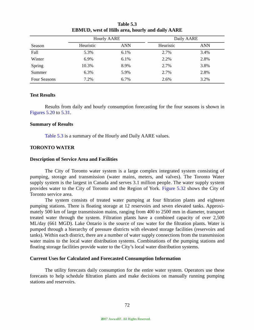
Test Results
Results from daily and hourly consumption forecasting for the four seasons is shown inFigures 5.20 to 5.31.
Summary of Results
Table 5.3 is a summary of the Hourly and Daily AARE values.
TORONTO WATER
Description of Service Area and Facilities
The City of Toronto water system is a large complex integrated system consisting ofpumping, storage and transmission (water mains, meters, and valves). The Toronto Watersupply system is the largest in Canada and serves 3.1 million people. The water supply systemprovides water to the City of Toronto and the Region of York. Figure 5.32 shows the City ofToronto service area.
The system consists of treated water pumping at four filtration plants and eighteenpumping stations. There is floating storage at 12 reservoirs and seven elevated tanks. Approxi-mately 500 km of large transmission mains, ranging from 400 to 2500 mm in diameter, transporttreated water through the system. Filtration plants have a combined capacity of over 2,500ML/day (661 MGD). Lake Ontario is the source of raw water for the filtration plants. Water ispumped through a hierarchy of pressure districts with elevated storage facilities (reservoirs andtanks). Within each district, there are a number of water supply connections from the transmissionwater mains to the local water distribution systems. Combinations of the pumping stations andfloating storage facilities provide water to the City’s local water distribution systems.
Current Uses for Calculated and Forecasted Consumption Information
The utility forecasts daily consumption for the entire water system. Operators use theseforecasts to help schedule filtration plants and make decisions on manually running pumpingstations and reservoirs.
Table 5.3EBMUD, west of Hills area, hourly and daily AARE
Season
Hourly AARE Daily AARE
Heuristic ANN Heuristic ANN
Fall 5.3% 6.1% 2.7% 3.4%
Winter 6.9% 6.1% 2.2% 2.8%
Spring 10.3% 8.9% 2.7% 3.8%
Summer 6.3% 5.9% 2.7% 2.8%
Four Seasons 7.2% 6.7% 2.6% 3.2%
72
©2007 AwwaRF. All Rights Reserved.
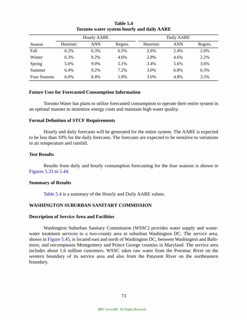
Future Uses for Forecasted Consumption Information
Toronto Water has plans to utilize forecasted consumption to operate their entire system inan optimal manner to minimize energy costs and maintain high water quality.
Formal Definition of STCF Requirements
Hourly and daily forecasts will be generated for the entire system. The AARE is expectedto be less than 10% for the daily forecasts. The forecasts are expected to be sensitive to variationsin air temperature and rainfall.
Test Results
Results from daily and hourly consumption forecasting for the four seasons is shown inFigures 5.33 to 5.44.
Summary of Results
Table 5.4 is a summary of the Hourly and Daily AARE values.
WASHINGTON SUBURBAN SANITARY COMMISSION
Description of Service Area and Facilities
Washington Suburban Sanitary Commission (WSSC) provides water supply and waste-water treatment services to a two-county area in suburban Washington DC. The service area,shown in Figure 5.45, is located east and north of Washington DC, between Washington and Balti-more, and encompasses Montgomery and Prince George counties in Maryland. The service areaincludes about 1.6 million customers. WSSC takes raw water from the Potomac River on thewestern boundary of its service area and also from the Patuxent River on the northeasternboundary.
Table 5.4Toronto water system hourly and daily AARE
Season
Hourly AARE Daily AARE
Heuristic ANN Regres. Heuristic ANN Regres.
Fall 6.2% 6.3% 6.5% 2.6% 2.4% 2.0%
Winter 6.3% 9.2% 4.6% 2.8% 4.6% 2.2%
Spring 5.0% 9.0% 5.1% 3.4% 5.6% 3.6%
Summer 6.4% 9.2% 7.2% 3.0% 6.8% 6.3%
Four Seasons 6.0% 8.4% 5.9% 3.0% 4.8% 3.5%
73
©2007 AwwaRF. All Rights Reserved.
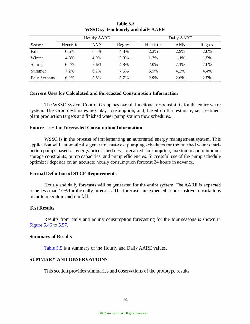
Current Uses for Calculated and Forecasted Consumption Information
The WSSC System Control Group has overall functional responsibility for the entire watersystem. The Group estimates next day consumption, and, based on that estimate, set treatmentplant production targets and finished water pump station flow schedules.
Future Uses for Forecasted Consumption Information
WSSC is in the process of implementing an automated energy management system. Thisapplication will automatically generate least-cost pumping schedules for the finished water distri-bution pumps based on energy price schedules, forecasted consumption, maximum and minimumstorage constraints, pump capacities, and pump efficiencies. Successful use of the pump scheduleoptimizer depends on an accurate hourly consumption forecast 24 hours in advance.
Formal Definition of STCF Requirements
Hourly and daily forecasts will be generated for the entire system. The AARE is expectedto be less than 10% for the daily forecasts. The forecasts are expected to be sensitive to variationsin air temperature and rainfall.
Test Results
Results from daily and hourly consumption forecasting for the four seasons is shown inFigure 5.46 to 5.57.
Summary of Results
Table 5.5 is a summary of the Hourly and Daily AARE values.
SUMMARY AND OBSERVATIONS
This section provides summaries and observations of the prototype results.
Table 5.5WSSC system hourly and daily AARE
Season
Hourly AARE Daily AARE
Heuristic ANN Regres. Heuristic ANN Regres.
Fall 6.6% 6.4% 4.8% 2.3% 2.9% 2.0%
Winter 4.8% 4.9% 5.8% 1.7% 1.1% 1.5%
Spring 6.2% 5.6% 4.8% 2.0% 2.1% 2.0%
Summer 7.2% 6.2% 7.5% 5.5% 4.2% 4.4%
Four Seasons 6.2% 5.8% 5.7% 2.9% 2.6% 2.5%
74
©2007 AwwaRF. All Rights Reserved.
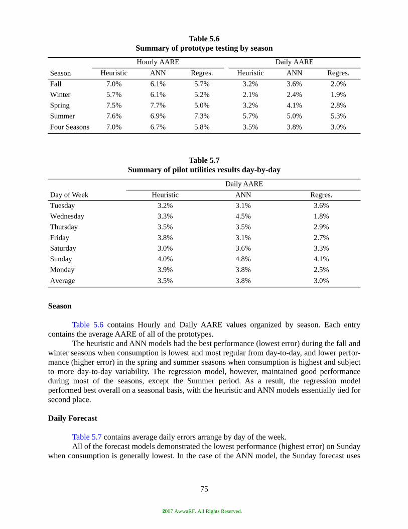
Season
Table 5.6 contains Hourly and Daily AARE values organized by season. Each entrycontains the average AARE of all of the prototypes.
The heuristic and ANN models had the best performance (lowest error) during the fall andwinter seasons when consumption is lowest and most regular from day-to-day, and lower perfor-mance (higher error) in the spring and summer seasons when consumption is highest and subjectto more day-to-day variability. The regression model, however, maintained good performanceduring most of the seasons, except the Summer period. As a result, the regression modelperformed best overall on a seasonal basis, with the heuristic and ANN models essentially tied forsecond place.
Daily Forecast
Table 5.7 contains average daily errors arrange by day of the week.All of the forecast models demonstrated the lowest performance (highest error) on Sunday
when consumption is generally lowest. In the case of the ANN model, the Sunday forecast uses
Table 5.6Summary of prototype testing by season
Season
Hourly AARE Daily AARE
Heuristic ANN Regres. Heuristic ANN Regres.
Fall 7.0% 6.1% 5.7% 3.2% 3.6% 2.0%
Winter 5.7% 6.1% 5.2% 2.1% 2.4% 1.9%
Spring 7.5% 7.7% 5.0% 3.2% 4.1% 2.8%
Summer 7.6% 6.9% 7.3% 5.7% 5.0% 5.3%
Four Seasons 7.0% 6.7% 5.8% 3.5% 3.8% 3.0%
Table 5.7Summary of pilot utilities results day-by-day
Day of Week
Daily AARE
Heuristic ANN Regres.
Tuesday 3.2% 3.1% 3.6%
Wednesday 3.3% 4.5% 1.8%
Thursday 3.5% 3.5% 2.9%
Friday 3.8% 3.1% 2.7%
Saturday 3.0% 3.6% 3.3%
Sunday 4.0% 4.8% 4.1%
Monday 3.9% 3.8% 2.5%
Average 3.5% 3.8% 3.0%
75
©2007 AwwaRF. All Rights Reserved.
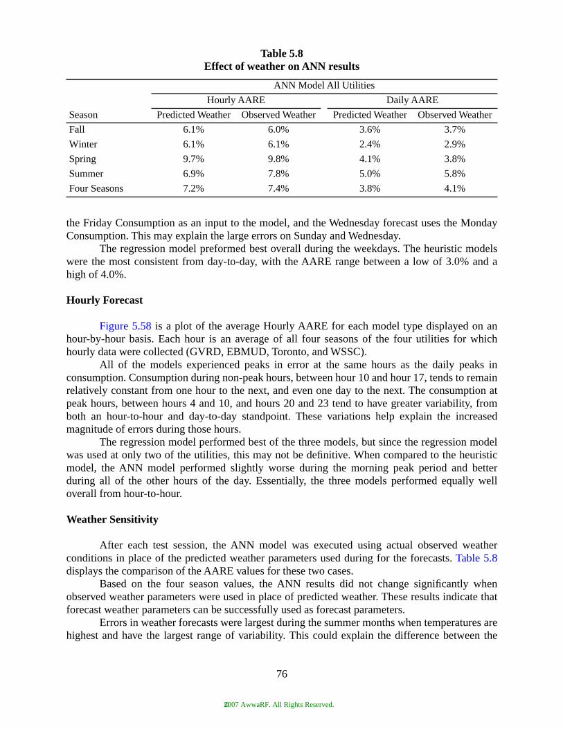
the Friday Consumption as an input to the model, and the Wednesday forecast uses the MondayConsumption. This may explain the large errors on Sunday and Wednesday.
The regression model preformed best overall during the weekdays. The heuristic modelswere the most consistent from day-to-day, with the AARE range between a low of 3.0% and ahigh of 4.0%.
Hourly Forecast
Figure 5.58 is a plot of the average Hourly AARE for each model type displayed on anhour-by-hour basis. Each hour is an average of all four seasons of the four utilities for whichhourly data were collected (GVRD, EBMUD, Toronto, and WSSC).
All of the models experienced peaks in error at the same hours as the daily peaks inconsumption. Consumption during non-peak hours, between hour 10 and hour 17, tends to remainrelatively constant from one hour to the next, and even one day to the next. The consumption atpeak hours, between hours 4 and 10, and hours 20 and 23 tend to have greater variability, fromboth an hour-to-hour and day-to-day standpoint. These variations help explain the increasedmagnitude of errors during those hours.
The regression model performed best of the three models, but since the regression modelwas used at only two of the utilities, this may not be definitive. When compared to the heuristicmodel, the ANN model performed slightly worse during the morning peak period and betterduring all of the other hours of the day. Essentially, the three models performed equally welloverall from hour-to-hour.
Weather Sensitivity
After each test session, the ANN model was executed using actual observed weatherconditions in place of the predicted weather parameters used during for the forecasts. Table 5.8displays the comparison of the AARE values for these two cases.
Based on the four season values, the ANN results did not change significantly whenobserved weather parameters were used in place of predicted weather. These results indicate thatforecast weather parameters can be successfully used as forecast parameters.
Errors in weather forecasts were largest during the summer months when temperatures arehighest and have the largest range of variability. This could explain the difference between the
Table 5.8Effect of weather on ANN results
Season
ANN Model All Utilities
Hourly AARE Daily AARE
Predicted Weather Observed Weather Predicted Weather Observed Weather
Fall 6.1% 6.0% 3.6% 3.7%
Winter 6.1% 6.1% 2.4% 2.9%
Spring 9.7% 9.8% 4.1% 3.8%
Summer 6.9% 7.8% 5.0% 5.8%
Four Seasons 7.2% 7.4% 3.8% 4.1%
76
©2007 AwwaRF. All Rights Reserved.

Predicted/Observed results during the summer. However, it is not clear why the ANN model,trained using observed historical data, would generally perform better using predicted weatherinputs. Here are two possible explanations for this behavior.
First, the weather parameters have an impact on consumption, but the correlation may notbe as strong as with historical consumption. The models may tolerate errors in temperature valuesof several degrees and still provide accurate forecast results.
Second, consumption by utility customers may be driven more by what the customerthinks the weather is going to be and less on the actual weather. For example, a home owner maywater their lawn based on the prediction of high temperatures whether or not the temperaturesactually increase.
The second explanation would be difficult to confirm since “weather forecasts” are neversaved in historical databases. However, the “psychology of water consumption” tends to make theimpact of weather on consumption forecasting more complex than expected.
Location
An effort was made to select utilities for prototyping with different geographical locationsand different weather patterns. Although the utilities were spread across North America, all werelocated in either the northern parts of the United States or southern parts of Canada. All of the util-ities were also close to large bodies of water that may have affected their weather in similar ways.None of the utilities experienced extremes in temperature or precipitation that are experienced byutilities in the West, Southwest, or Southeast of the United States.
For all of the utilities, the primary predictor of consumption was previous consumption.Temperature (daily maximum and minimum) and day of the week also correlated well withconsumption, but not as strongly as previous consumption. Other weather parameters (windspeed, wind direction, cloud cover, UV Index) had no correlation.
Both Seattle (SPU) and Washington, DC (WSSC) receive a great deal of annual precipita-tion. Consequently, the ANN model was found to correlate well with precipitation at these two sites.
At EBMUD, the ANN model correlated better with a three-day accumulated precipitationparameter. This type of parameter converts “instantaneous” precipitation events into a longerlasting parameter. This implies that precipitation events at EBMUD have an impact on consump-tion for several days beyond the precipitation event.
The GVRD and Toronto ANN models had low correlation to precipitation. Dew point, hada much higher correlation, and was used in lieu of precipitation. It is not certain whether dewpoint provided sufficient precipitation prediction, or merely reinforced the affect ofmaximum/minimum temperature variations. However, dew point forecasts were more reliablethan precipitation forecasts and may be an adequate substitute in some cases.
Data Quality
All three model types; heuristic, ANN, and regression, depend on accurate consumptiondata for both preparation and execution of the forecast models. Any gaps or errors in the historicaldata set, especially in the cases of the heuristic and regression models can make forecasting eitherdifficult or impossible. The ANN model can tolerate some errors since the typical training data setcontains a year of data. However, the historical data set should be reviewed and corrected beforetraining the model in order to insure the best possible results.
77
©2007 AwwaRF. All Rights Reserved.

Once prepared, the models also need accurate recent consumption data for the final fore-cast. Again, accurate and complete consumption is critical for an accurate forecast. Use of a dataquality software program may be advisable to review data prior to being used in a forecast toeither correct bad values or alert the administrator regarding data problems.
Another issue regarding data quality is data precision. A single consumption value may becalculated from several sampled values of flow and reservoir levels. Each sampled value has alevel of precision based on the precision of the measuring device (flow meter, reservoir levelsensor), precision of the communication protocol, and precision of the data storage element. Noforecast can be better than the data used to create the forecast. Therefore attention should be paidto regular calibration of sensors and improvement of data precision in communication protocolsand data storage.
Errors can also be introduced in the forecasts via the weather data. Typically, actualtemperature conditions are within a few degrees of a forecast made 24 hours earlier. However,sensor problems, data-entry, and other human errors can introduce errors that will dramaticallyaffect the forecast.
Daylight Savings Time must also be taken into account, especially for the ANN modelsthat use data that span both Standard and Daylight Savings time periods. A convention must beestablished to insure that the forecasts match the temporal patterns of the local customers to insurethat the forecasts are synchronized. A shift by a single hour between the forecast and actualconsumptions can result in ARE values in excess of 30% during the peak consumption hours.
Figure 5.1 SPU service area
78
©2007 AwwaRF. All Rights Reserved.
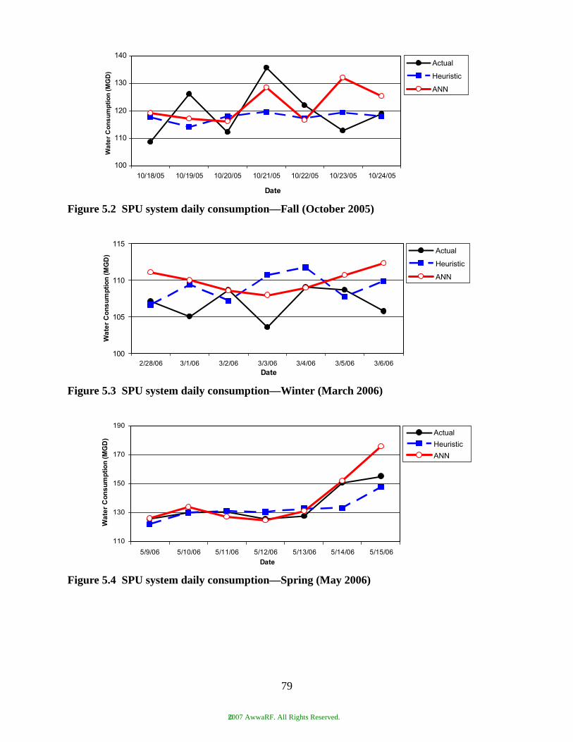
Figure 5.2 SPU system daily consumption—Fall (October 2005)
Figure 5.3 SPU system daily consumption—Winter (March 2006)
Figure 5.4 SPU system daily consumption—Spring (May 2006)
100
110
120
130
140
10/18/05 10/19/05 10/20/05 10/21/05 10/22/05 10/23/05 10/24/05
Date
)D
GM(
noit
pm
us
no
C ret
aW
Actual
Heuristic
ANN
100
105
110
115
2/28/06 3/1/06 3/2/06 3/3/06 3/4/06 3/5/06 3/6/06Date
)D
GM(
noit
pm
us
no
C ret
aW
Actual
Heuristic
ANN
110
130
150
170
190
5/9/06 5/10/06 5/11/06 5/12/06 5/13/06 5/14/06 5/15/06
Date
)D
GM(
noit
pm
us
no
C ret
aW
Actual
Heuristic
ANN
79
©2007 AwwaRF. All Rights Reserved.
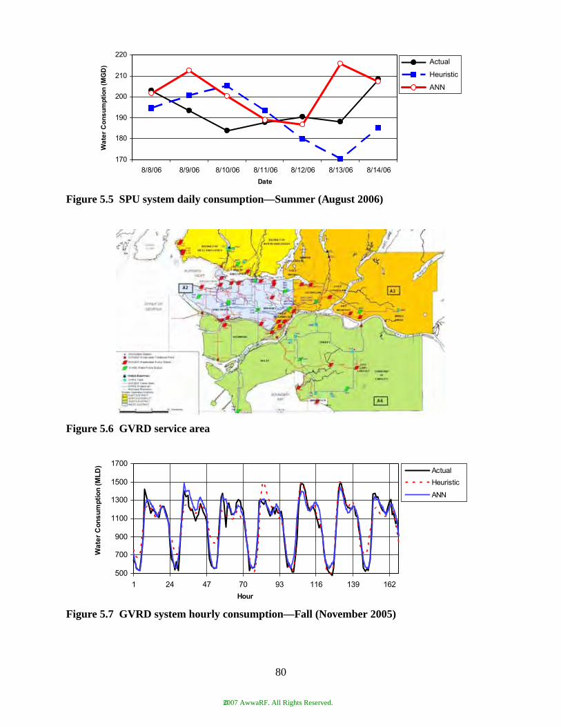
Figure 5.5 SPU system daily consumption—Summer (August 2006)
Figure 5.6 GVRD service area
Figure 5.7 GVRD system hourly consumption—Fall (November 2005)
170
180
190
200
210
220
8/8/06 8/9/06 8/10/06 8/11/06 8/12/06 8/13/06 8/14/06
Date
)D
GM(
noit
pm
us
no
C ret
aW
Actual
Heuristic
ANN
500
700
900
1100
1300
1500
1700
1 24 47 70 93 116 139 162
Hour
)D
LM(
noit
pm
us
no
C ret
aW
Actual
Heuristic
ANN
80
©2007 AwwaRF. All Rights Reserved.
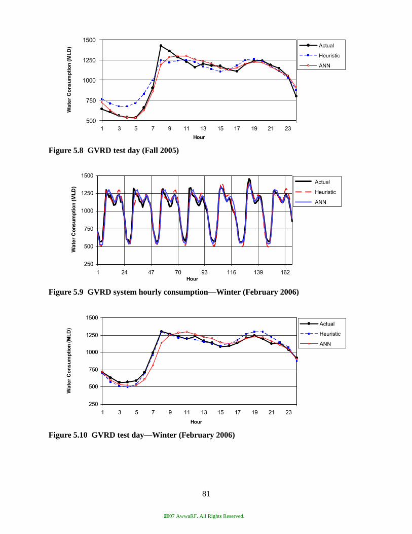
Figure 5.8 GVRD test day (Fall 2005)
Figure 5.9 GVRD system hourly consumption—Winter (February 2006)
Figure 5.10 GVRD test day—Winter (February 2006)
500
750
1000
1250
1500
1 3 5 7 9 11 13 15 17 19 21 23
Hour
)D
LM(
noit
pm
us
no
C ret
aW
Actual
Heuristic
ANN
250
500
750
1000
1250
1500
1 24 47 70 93 116 139 162Hour
)D
LM(
noit
pm
us
no
C ret
aW
Actual
Heuristic
ANN
250
500
750
1000
1250
1500
1 3 5 7 9 11 13 15 17 19 21 23
Hour
)D
LM(
noit
pm
us
no
C ret
aW
Actual
Heuristic
ANN
81
©2007 AwwaRF. All Rights Reserved.
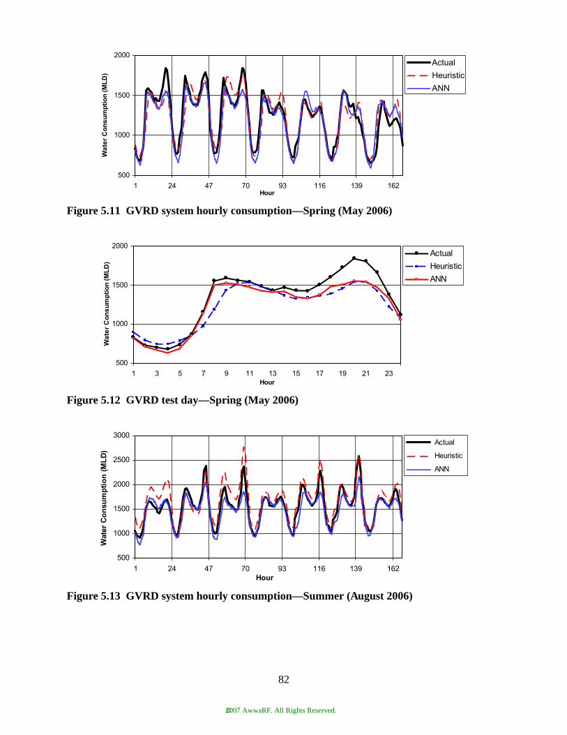
Figure 5.11 GVRD system hourly consumption—Spring (May 2006)
Figure 5.12 GVRD test day—Spring (May 2006)
Figure 5.13 GVRD system hourly consumption—Summer (August 2006)
500
1000
1500
2000
1 24 47 70 93 116 139 162Hour
)D
LM(
noit
pm
us
no
C ret
aW
Actual
Heuristic
ANN
500
1000
1500
2000
1 3 5 7 9 11 13 15 17 19 21 23Hour
)D
LM(
noit
pm
us
no
C ret
aW
Actual
Heuristic
ANN
500
1000
1500
2000
2500
3000
1 24 47 70 93 116 139 162Hour
)D
LM(
noit
pm
usn
oC reta
W
Actual
Heuristic
ANN
82
©2007 AwwaRF. All Rights Reserved.
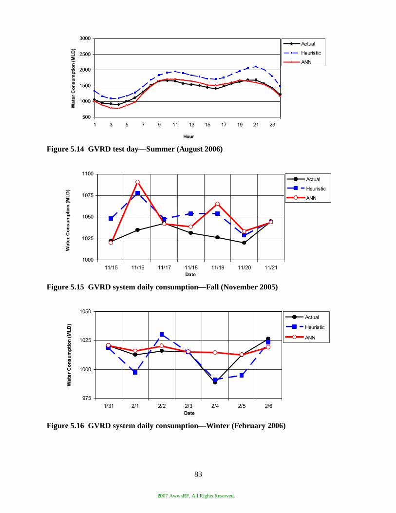
Figure 5.14 GVRD test day—Summer (August 2006)
Figure 5.15 GVRD system daily consumption—Fall (November 2005)
Figure 5.16 GVRD system daily consumption—Winter (February 2006)
500
1000
1500
2000
2500
3000
1 3 5 7 9 11 13 15 17 19 21 23
Hour
)D
LM(
noit
pm
us
no
C ret
aW
Actual
Heuristic
ANN
1000
1025
1050
1075
1100
11/15 11/16 11/17 11/18 11/19 11/20 11/21Date
)D
LM(
noit
pm
us
no
C ret
aW
Actual
Heuristic
ANN
975
1000
1025
1050
1/31 2/1 2/2 2/3 2/4 2/5 2/6Date
)D
LM(
noit
pm
us
no
C ret
aW
Actual
Heuristic
ANN
83
©2007 AwwaRF. All Rights Reserved.
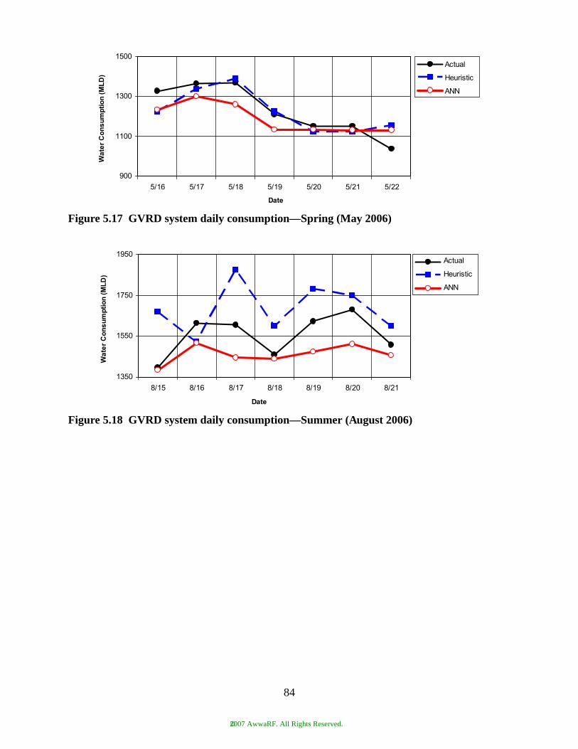
Figure 5.17 GVRD system daily consumption—Spring (May 2006)
Figure 5.18 GVRD system daily consumption—Summer (August 2006)
900
1100
1300
1500
5/16 5/17 5/18 5/19 5/20 5/21 5/22
Date
)D
LM(
noit
pm
us
no
C ret
aW
Actual
Heuristic
ANN
1350
1550
1750
1950
8/15 8/16 8/17 8/18 8/19 8/20 8/21
Date
)D
LM(
noit
pm
us
no
C ret
aW
Actual
Heuristic
ANN
84
©2007 AwwaRF. All Rights Reserved.
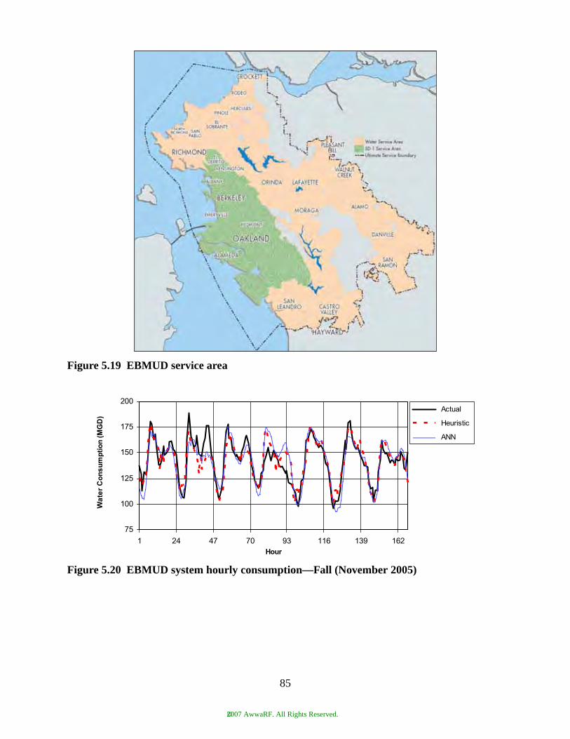
Figure 5.19 EBMUD service area
Figure 5.20 EBMUD system hourly consumption—Fall (November 2005)
75
100
125
150
175
200
1 24 47 70 93 116 139 162Hour
)D
GM(
noit
pm
us
no
C ret
aW
Actual
Heuristic
ANN
85
©2007 AwwaRF. All Rights Reserved.
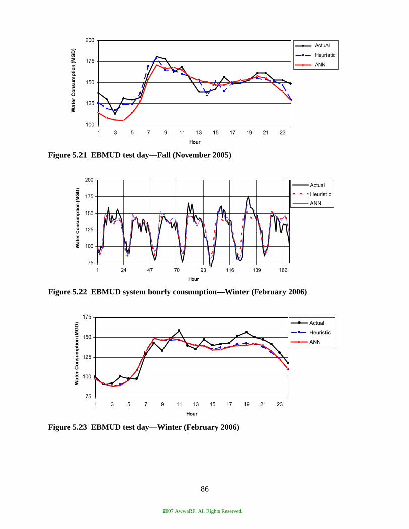
Figure 5.21 EBMUD test day—Fall (November 2005)
Figure 5.22 EBMUD system hourly consumption—Winter (February 2006)
Figure 5.23 EBMUD test day—Winter (February 2006)
100
125
150
175
200
1 3 5 7 9 11 13 15 17 19 21 23
Hour
)D
GM(
noit
pm
us
no
C ret
aW
Actual
Heuristic
ANN
75
100
125
150
175
200
1 24 47 70 93 116 139 162
Hour
)D
GM(
noit
pm
us
no
C ret
aW
Actual
Heuristic
ANN
75
100
125
150
175
1 3 5 7 9 11 13 15 17 19 21 23
Hour
)D
GM(
noit
pm
us
no
C ret
aW
Actual
Heuristic
ANN
86
©2007 AwwaRF. All Rights Reserved.
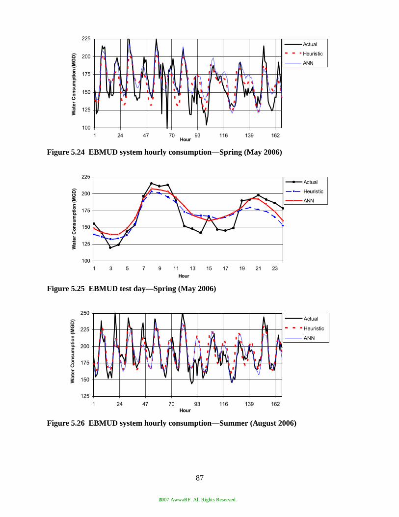
Figure 5.24 EBMUD system hourly consumption—Spring (May 2006)
Figure 5.25 EBMUD test day—Spring (May 2006)
Figure 5.26 EBMUD system hourly consumption—Summer (August 2006)
100
125
150
175
200
225
1 24 47 70 93 116 139 162Hour
)D
GM(
noit
pm
us
no
C ret
aW
Actual
Heuristic
ANN
100
125
150
175
200
225
1 3 5 7 9 11 13 15 17 19 21 23
Hour
)D
GM(
noit
pm
us
no
C ret
aW
Actual
Heuristic
ANN
125
150
175
200
225
250
1 24 47 70 93 116 139 162Hour
)D
GM(
noit
pm
us
no
C ret
aW
Actual
Heuristic
ANN
87
©2007 AwwaRF. All Rights Reserved.
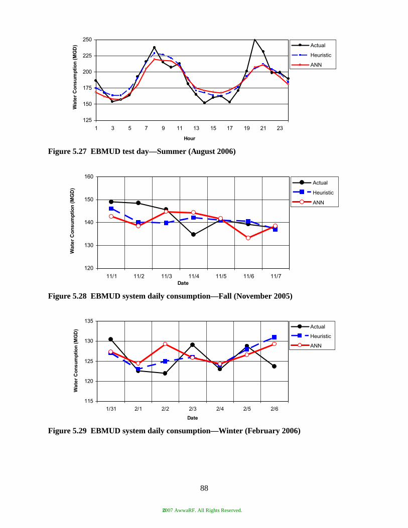
Figure 5.27 EBMUD test day—Summer (August 2006)
Figure 5.28 EBMUD system daily consumption—Fall (November 2005)
Figure 5.29 EBMUD system daily consumption—Winter (February 2006)
125
150
175
200
225
250
1 3 5 7 9 11 13 15 17 19 21 23
Hour
)D
GM(
noit
pm
us
no
C ret
aW
Actual
Heuristic
ANN
120
130
140
150
160
11/1 11/2 11/3 11/4 11/5 11/6 11/7Date
)D
GM(
noit
pm
us
no
C ret
aW
Actual
Heuristic
ANN
115
120
125
130
135
1/31 2/1 2/2 2/3 2/4 2/5 2/6
Date
)D
GM(
noit
pm
us
no
C ret
aW
Actual
Heuristic
ANN
88
©2007 AwwaRF. All Rights Reserved.
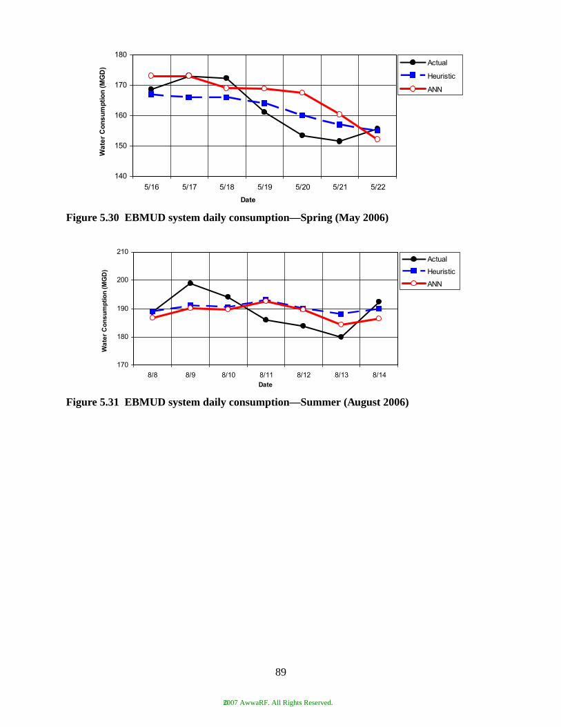
Figure 5.30 EBMUD system daily consumption—Spring (May 2006)
Figure 5.31 EBMUD system daily consumption—Summer (August 2006)
140
150
160
170
180
5/16 5/17 5/18 5/19 5/20 5/21 5/22
Date
)D
GM(
noit
pm
us
no
C ret
aW
Actual
Heuristic
ANN
170
180
190
200
210
8/8 8/9 8/10 8/11 8/12 8/13 8/14Date
)D
GM(
noit
pm
us
no
C ret
aW
Actual
Heuristic
ANN
89
©2007 AwwaRF. All Rights Reserved.
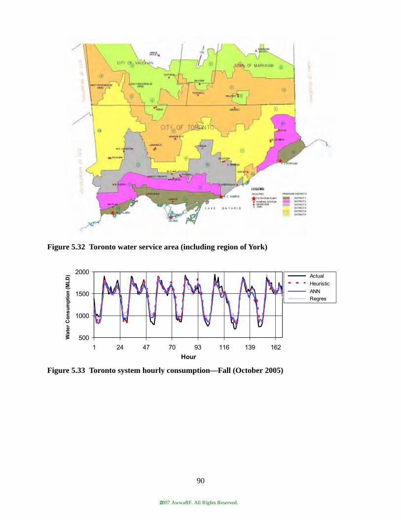
Figure 5.32 Toronto water service area (including region of York)
Figure 5.33 Toronto system hourly consumption—Fall (October 2005)
500
1000
1500
2000
1 24 47 70 93 116 139 162
Hour
Actual
Heuristic
ANNRegres
)D
LM(
noit
pm
us
no
C ret
aW
90
©2007 AwwaRF. All Rights Reserved.
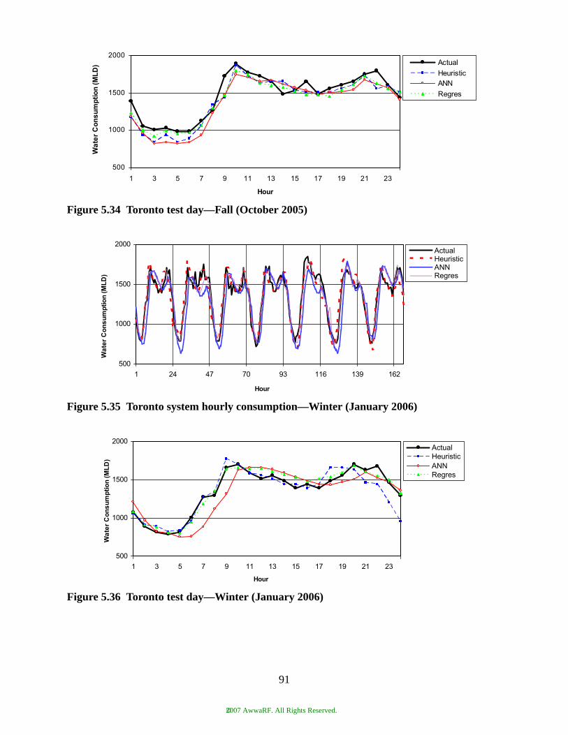
Figure 5.34 Toronto test day—Fall (October 2005)
Figure 5.35 Toronto system hourly consumption—Winter (January 2006)
Figure 5.36 Toronto test day—Winter (January 2006)
500
1000
1500
2000
1 3 5 7 9 11 13 15 17 19 21 23
Hour
)D
LM(
noit
pm
us
no
C ret
aW
Actual
HeuristicANN
Regres
500
1000
1500
2000
1 24 47 70 93 116 139 162
Hour
)D
LM(
noit
pm
us
no
C ret
aW
ActualHeuristicANNRegres
500
1000
1500
2000
1 3 5 7 9 11 13 15 17 19 21 23
Hour
)D
LM(
noit
pm
us
no
C ret
aW
ActualHeuristicANNRegres
91
©2007 AwwaRF. All Rights Reserved.
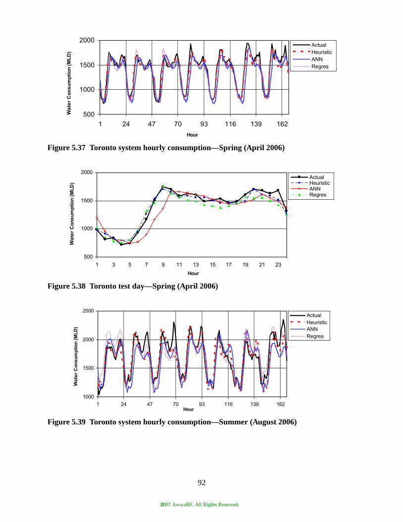
Figure 5.37 Toronto system hourly consumption—Spring (April 2006)
Figure 5.38 Toronto test day—Spring (April 2006)
Figure 5.39 Toronto system hourly consumption—Summer (August 2006)
500
1000
1500
2000
1 24 47 70 93 116 139 162
Hour
)D
LM(
noit
pm
us
no
C ret
aW
ActualHeuristicANNRegres
500
1000
1500
2000
1 3 5 7 9 11 13 15 17 19 21 23
Hour
)D
LM(
noit
pm
us
no
C ret
aW
ActualHeuristicANNRegres
1000
1500
2000
2500
1 24 47 70 93 116 139 162Hour
)D
LM(
noit
pm
us
no
C ret
aW
ActualHeuristicANNRegres
92
©2007 AwwaRF. All Rights Reserved.
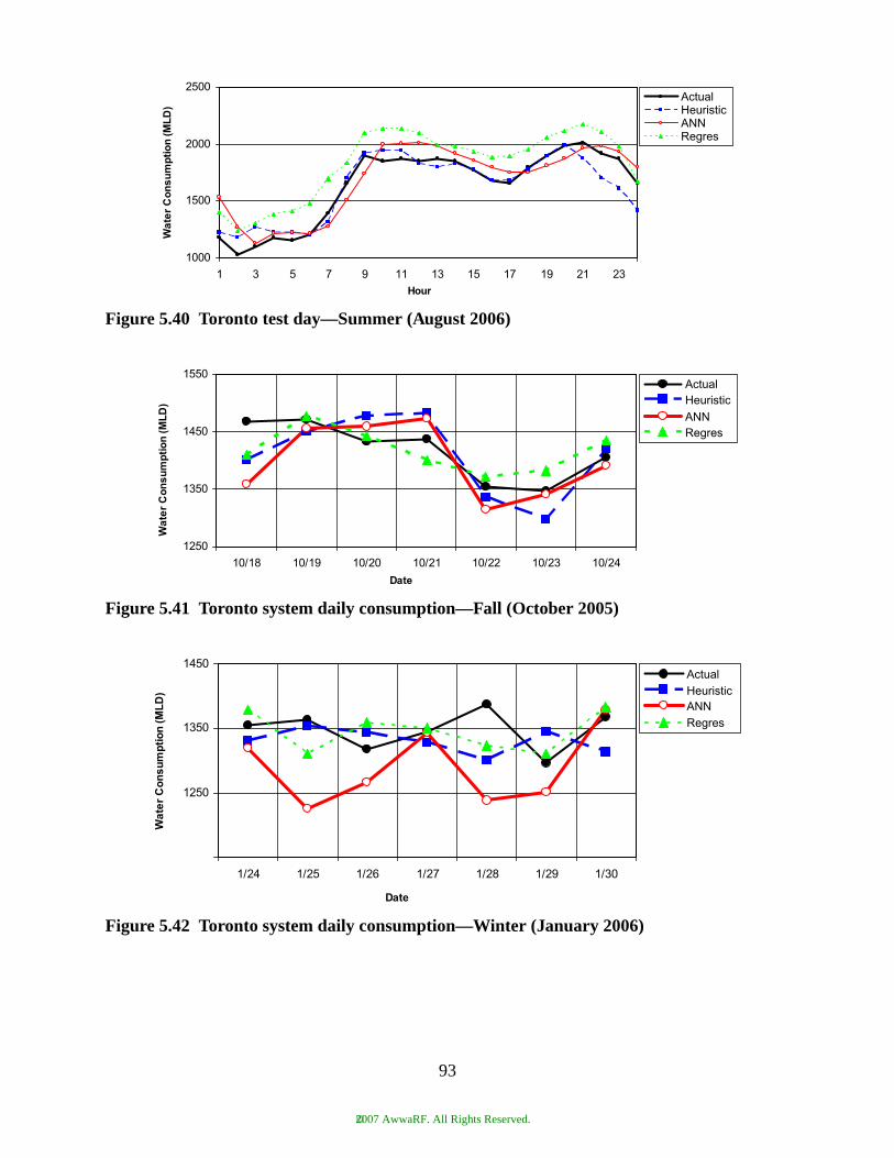
Figure 5.40 Toronto test day—Summer (August 2006)
Figure 5.41 Toronto system daily consumption—Fall (October 2005)
Figure 5.42 Toronto system daily consumption—Winter (January 2006)
1000
1500
2000
2500
1 3 5 7 9 11 13 15 17 19 21 23
Hour
)D
LM(
noit
pm
us
no
C ret
aW
ActualHeuristicANNRegres
1250
1350
1450
1550
10/18 10/19 10/20 10/21 10/22 10/23 10/24
Date
)D
LM(
noit
pm
us
no
C ret
aW
ActualHeuristic
ANNRegres
1150
1250
1350
1450
1/24 1/25 1/26 1/27 1/28 1/29 1/30
Date
)D
LM(
noit
pm
us
no
C ret
aW
ActualHeuristicANNRegres
93
©2007 AwwaRF. All Rights Reserved.
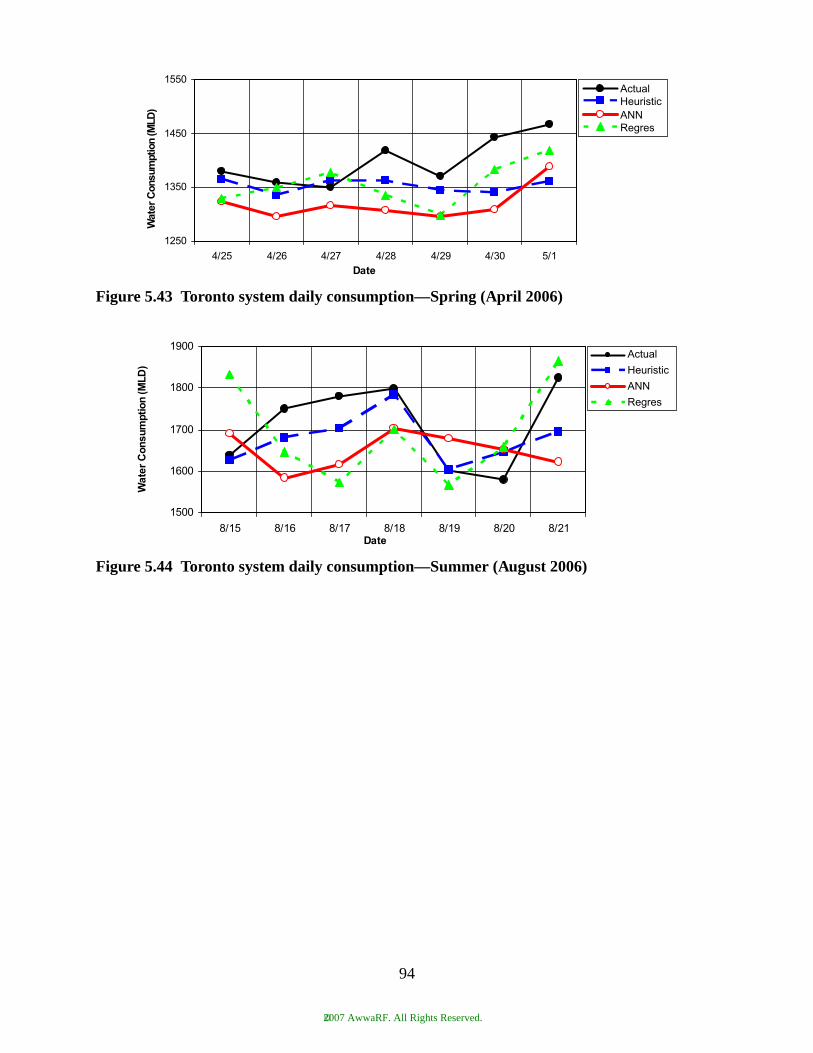
Figure 5.43 Toronto system daily consumption—Spring (April 2006)
Figure 5.44 Toronto system daily consumption—Summer (August 2006)
1250
1350
1450
1550
4/25 4/26 4/27 4/28 4/29 4/30 5/1
Date
)DL
M( noitpmusno
C retaW
ActualHeuristicANNRegres
1500
1600
1700
1800
1900
8/15 8/16 8/17 8/18 8/19 8/20 8/21Date
)DL
M( noitpmusno
C retaW
Actual
Heuristic
ANN
Regres
94
©2007 AwwaRF. All Rights Reserved.
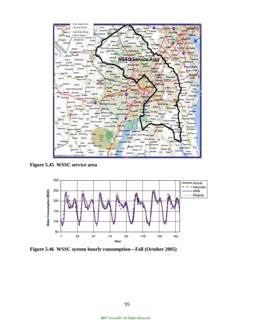
Figure 5.45 WSSC service area
Figure 5.46 WSSC system hourly consumption—Fall (October 2005)
50
100
150
200
250
300
1 24 47 70 93 116 139 162
Hour
)D
GM(
noit
pm
us
no
C ret
aW
ActualHeuristicANNRegres
95
©2007 AwwaRF. All Rights Reserved.
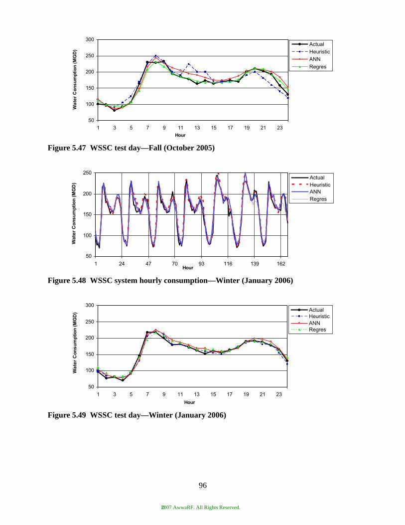
Figure 5.47 WSSC test day—Fall (October 2005)
Figure 5.48 WSSC system hourly consumption—Winter (January 2006)
Figure 5.49 WSSC test day—Winter (January 2006)
50
100
150
200
250
300
1 3 5 7 9 11 13 15 17 19 21 23
Hour
)D
GM(
noit
pm
us
no
C ret
aW
ActualHeuristicANNRegres
50
100
150
200
250
1 24 47 70 93 116 139 162Hour
)D
GM(
noit
pm
us
no
C ret
aW
ActualHeuristicANNRegres
50
100
150
200
250
300
1 3 5 7 9 11 13 15 17 19 21 23
Hour
)D
GM(
noit
pm
us
no
C ret
aW
ActualHeuristicANNRegres
96
©2007 AwwaRF. All Rights Reserved.
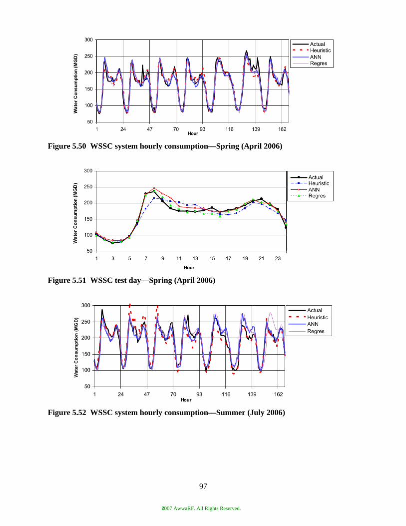
Figure 5.50 WSSC system hourly consumption—Spring (April 2006)
Figure 5.51 WSSC test day—Spring (April 2006)
Figure 5.52 WSSC system hourly consumption—Summer (July 2006)
50
100
150
200
250
300
1 24 47 70 93 116 139 162Hour
)D
GM(
noit
pm
us
no
C ret
aW
ActualHeuristicANNRegres
50
100
150
200
250
300
1 3 5 7 9 11 13 15 17 19 21 23
Hour
)D
GM(
noit
pm
us
no
C ret
aW
ActualHeuristicANNRegres
50
100
150
200
250
300
1 24 47 70 93 116 139 162Hour
)D
GM(
noit
pm
usn
oC reta
W
ActualHeuristicANNRegres
97
©2007 AwwaRF. All Rights Reserved.
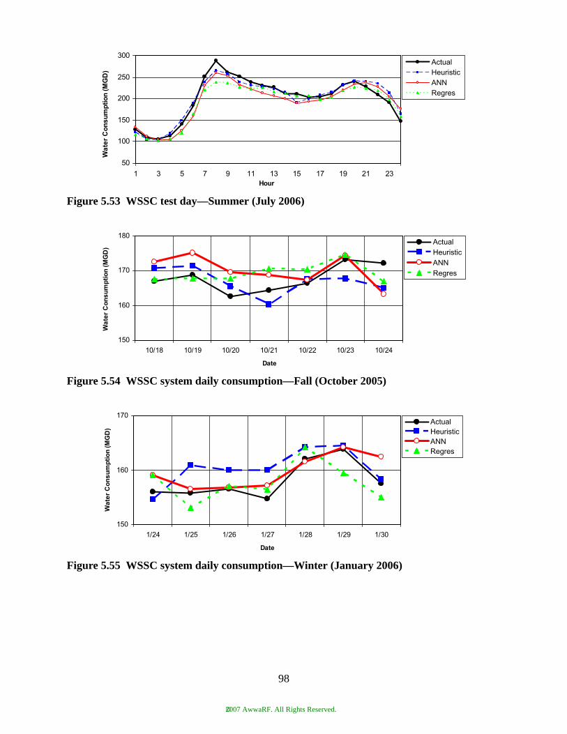
Figure 5.53 WSSC test day—Summer (July 2006)
Figure 5.54 WSSC system daily consumption—Fall (October 2005)
Figure 5.55 WSSC system daily consumption—Winter (January 2006)
50
100
150
200
250
300
1 3 5 7 9 11 13 15 17 19 21 23Hour
)D
GM(
noit
pm
us
no
C ret
aW
ActualHeuristicANNRegres
150
160
170
180
10/18 10/19 10/20 10/21 10/22 10/23 10/24
Date
)D
GM(
noit
pm
us
no
C ret
aW
ActualHeuristicANNRegres
150
160
170
1/24 1/25 1/26 1/27 1/28 1/29 1/30
Date
)D
GM(
noit
pm
us
no
C ret
aW
ActualHeuristicANNRegres
98
©2007 AwwaRF. All Rights Reserved.
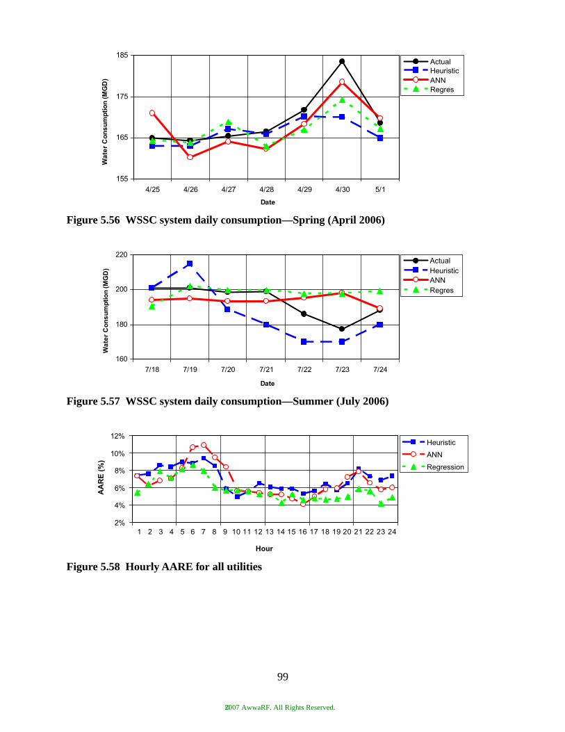
Figure 5.56 WSSC system daily consumption—Spring (April 2006)
Figure 5.57 WSSC system daily consumption—Summer (July 2006)
Figure 5.58 Hourly AARE for all utilities
155
165
175
185
4/25 4/26 4/27 4/28 4/29 4/30 5/1
Date
)D
GM(
noit
pm
us
no
C ret
aW
ActualHeuristicANNRegres
160
180
200
220
7/18 7/19 7/20 7/21 7/22 7/23 7/24
Date
)D
GM(
noit
pm
us
no
C ret
aW
ActualHeuristicANNRegres
2%
4%
6%
8%
10%
12%
1 2 3 4 5 6 7 8 9 10 11 12 13 14 15 16 17 18 19 20 21 22 23 24
Hour
AA
RE
(%
)
Heuristic
ANN
Regression
99
©2007 AwwaRF. All Rights Reserved.

©2007 AwwaRF. All Rights Reserved.

CHAPTER 6 ELECTRIC UTILITY EXPERIENCE AND VALUE
OF FORECASTING ACCURACY
This section of the report reviews the necessary level of commitment and value to achieve ahigh level of accuracy in short-term consumption forecasting. Electric utilities have substantiallymore experience in STCF systems than do water utilities so their experience is cited as a valuablereference. A hypothetical example which relates the cost of forecasting error to optimized control ofpumping to minimize energy cost is also provided. Together, these examples should assist water util-ities in their efforts to evaluate the performance and value of STCF systems.
ELECTRIC UTILITY EXPERIENCE WITH SYSTEM LOAD FORECASTING (SLF) PERFORMANCE
The following provides a perspective of SLF systems and forecasting techniques used byelectrical utilities.
Electric utilities prepare short-term forecasts from both a system and an area perspective.
APPLICATION OF SLF SYSTEMS
Most short-term System Load Forecasting (SLF) software currently available in themarketplace can handle forecasting for multiple areas and multiple utility companies within onesystem. There are many reasons why utilities need to run SLF software for multiple areas. Specif-ically, for reliability reasons, utilities and Independent System Operators (ISOs) responsible forthe reliability of the system need to know the short-term load demand in certain local areas toensure that sufficient generation is produced locally. For example, in electrical islands like theCity of San Francisco, a certain portion of the generating capacity required to meet local demandneeds to be met by local resources, i.e., reliance from outside generating resources should be keptwithin limits. This means that it is important to know the short-term load forecast for the area ofSan Francisco to satisfy the operational requirement. Typically, all utility systems are divided inLocal Reliability Areas (LRAs) to better manage local reliability. Short-term load forecasting isrequired for all LRAs.
There are two typical ways to forecast short-term load demand in multiple areas. One is todevelop separate forecasting models for each well defined geographical area. For each subsystemweather and other data are required to support accurate short-term load forecasting. The sum of allthe subsystems’ load forecasts is the System Load Forecast (SLF) that is traditionally used forscheduling and commitment. The other approach is to develop models to forecast the SLF for theentire system, and then use Load Distribution Factors (LDFs) to calculate load forecasts at thelocal level. The Load Distribution Factors are the percentages of an individual areas’ loads withrespect to the whole system load; their values can be updated hourly, daily or weekly. LDFs canbe computed using planning methods from off-line power flow models or using real time datafrom the State Estimator (SE) of the EMS/SCADA system. These two methods can be used at thesame time. For example, for areas with weather information available, forecasting models can bedeveloped; while for areas without sufficient weather data, the LDF-based method is preferable.
101
©2007 AwwaRF. All Rights Reserved.

In general, the fundamental structure of load forecasting methodologies does not vary byapplication. However, certain features related to output processing functionality can be expanded toserve the requirements of specific applications for which load forecasts are used as inputs. Loadforecasting results can be presented at system level, areas level, or even at a bus level. The fore-casting results can also be presented jointly with other hourly data related to planning and sched-uling for generation, transmission and distribution; for example, the area load can be displayed withan area’s energy prices, generation, imported/exported energy, and transmission line usage percent-ages for the user to get a global view of the energy usage and associated prices for each area.
RESOLUTION OF SLF SYSTEMS
The forecast resolution depends on the application that requires the forecast. Typicalscheduling and resource commitment applications require hourly forecasts. In some countries,like Australia, the load forecast resolution for scheduling applications is half hourly. The timehorizon for these models varies from one day to one week. The short-term load forecasting soft-ware generates 24 hourly forecasts for each day and 168 hourly forecasts for up to one week.Annual chronological simulation models also require hourly loads forecast resolution. In additionto the hourly forecasts, it is a typical requirement to have forecasts for daily peak load and dailyminimal load for each day of forecasting in long-term chronological simulation models. Also day-ahead energy market clearing applications in most jurisdictions with deregulated energy marketsrequire hourly forecasts.
In recently deregulated energy markets in the U.S. and abroad, real time markets havebeen developed that require very short-term load forecasts. The granularity of these forecastsvaries from 5 minutes to 15 minutes. The accuracy requirements of these forecasts are very strictsince they drive the clearing of the real time markets that produce dispatch schedules for gener-ating resources and real time prices at various locations where loads and resources are settled. Insome cases weather forecasting data doesn’t match this level of resolution. Therefore, in thesecases the core models and algorithms are usually still hourly-based; however, the forecast valuesfor the sub-hour intervals are calculated by linear interpolation, or by using curve fitting based onthe average daily load profiles.
SLF ACCURACY
SLF accuracy requirements vary from one utility to another and from application to appli-cation. For scheduling and resource commitment applications that require hourly forecasts withtime horizon from one day to one week, the most significant factor that affects the SLF accuracyis the weather forecast accuracy. Weather related data are the most important input variables toSLF models, and inaccuracies in weather forecasts have a severe negative effect on the load fore-cast performance. For example for the state of California, sensitivity studies give credence to theclaim that one degree error in temperature during the summer months results in about 300 MWsystem load forecasting error.
The most widely used measurement index for evaluating forecasting accuracy in the elec-tric utility industry is Average Absolute Percentage Error, which is calculated as the following:
e(i) = 100 * |(Forecast(i) – Actual(i)) ÷ Actual| %,
102
©2007 AwwaRF. All Rights Reserved.

where i = 1,2, …, N, and N is the number of forecasts used for the performance evaluation.
Average Absolute Percentage Error for all samples, E, is defined as
E = [e(1) + e(2) + e(3) + ... + e(N)]/N
Typically, the acceptable forecasting accuracy for Average Absolute Percentage Errors isabout 2–2.5% when models are tested with actual weather data and historical load data for whichdata errors have been excluded. However, when models are used in the production environmentwith forecasted weather data, the average absolute percentage error is usually around 2.5–3%. Itshould be noted that in many published papers on load forecasting, the accuracies reported areless than 2%. These high performance levels on SLF accuracy result from well optimized modelswith parameters and dataset well calibrated for optimal performance for certain conditions.Furthermore, inmost cases these results are calculated from best-performed time periods withworst-performed days excluded from the dataset.
In some cases utilities use, in addition to the Average Absolute Percentage Error, thenumber of maximum errors over a period of time, such as a year. The reason is that the AverageAbsolute Percentage Error tends to mask large errors. A maximum error is defined as an error thatexceeds a certain threshold which is usually a percentage of the system load. The threshold issometimes updated to reflect the capacity of the biggest generating unit in the system.
COMMITMENT REQUIRED TO ACHIEVE ACCURACY BENCHMARKS
The up front cost of achieving SLF accuracies consistent with acceptable levels as previ-ously defined is significant. It involves the purchase of an acceptable software package that isusually based on advanced statistical methods or Neural Network techniques. The time needed todevelop and deploy a short-term load forecaster for a medium-size electric utility varies by thechosen overall software configuration as well as the detailed software modules that are required tosupport the baseline functionality. The typical modules used in a baseline, short-term load fore-caster include:
1. A numerical engine for performing numerical calculations, which could be based onthe neural networks, multivariate regression, or other algorithms. It performs modelsparameters estimation/training, and calculates forecasts on-line.
2. A database for storing, managing and processing data, and handling inputs/outputs forthe numerical engine.
3. Interfaces—There are two types of interfaces: user interface and data interfaces; theuser interface is used to command the software executions and to present the results;the data interface is used to collect and process input data for running the forecasting,such as that for weather data and for historical and real-time load data.
Development and implementation of these baseline modules of a short-term load forecasterrequire about a 12 to 14 person-months. If a utility/ISO decides to purchase an SLF softwarepackage it is expected that 7 person-months are required to calibrate, tune and optimize the perfor-mance of the short-term load forecaster. Further modifications for performance enhancements,training and stabilization of the software operation may need another 3 to 5 person-months.
103
©2007 AwwaRF. All Rights Reserved.

In addition to the baseline functionality of a short-term load forecaster, it may be required,depending on the specific system conditions, to develop and implement auxiliary software modulesto support the baseline load forecaster. Examples of such auxiliary software modules include:
1. Adaptive error feedback mechanisms2. Self-tuning parameter optimization 3. Automated load error detector4. Improved non-conforming load forecasting, such as pump storage forecasting5. Sub-area load forecasting capability6. Special forecasting capability to handle special events, holidays, etc.7. Implementation of customized meteorological models to minimize forecasting tem-
perature errors.
The ongoing support and maintenance is relatively high. It requires one to two full timestaff with substantial knowledge on analytical SLF techniques and system operational expertise.The SLF model needs to be constantly calibrated to reflect new data and system conditions.Furthermore, the SLF model is executed several times a day to reflect the latest weather condi-tions. As part of maintenance and software support and enhancements the SLF support staff needsto perform ongoing activities such as implementation of automated load error detector methodol-ogies, improving pump storage forecasts, optimization of self-tuning parameters, improvingweather forecasts, collection and maintenance of data for subsystem load forecasts, etc.
The value of SLF accuracy is very high. Sometimes due to lack of accurate load forecasts,utilities and ISOs are forced to commit expensive units at the last minute and purchase importpower at high prices. Furthermore, in deregulated energy markets, load forecasts drive theclearing of the energy markets. Errors in load forecast have a direct impact on the resulting loca-tional prices and the dispatch levels of generating resources. In addition to the economic burdenimposed on systems with poor load forecasts, SLF accuracy has a direct impact on the reliabilityof the system.
METHODS USED BY ELECTRIC UTILITIES FOR LOAD FORECASTING
Neural networks and regression based approach are the two most widely used forecastingmethods in the power utility industry today. Similar Day methods are based on heuristics. Theyare rarely used as stand alone methods today. Sometimes they are used in conjunction withnumerical algorithm-based models as a complement to augment the SLF results. Implementationpercentages for each approach are not currently available, nor are surveys that summarize suchstatistical results. Based on anecdotal and empirical evidence, 60% of the currently used fore-casting methods for short-load forecasters are Neural Network-based, 30% are regression-basedand the rest are based on Similar Day methodologies.
Neural networks are currently considered the state-of-the-art of load forecast technologies.They have gained great popularity and acceptance in both industrial and academic circles. Neuralnetworks are essentially statistical devices for performing inductive inference. From the statisticalpoint of view they are analogous to nonparametric, nonlinear regression models. They are particu-larly useful to load forecasting, where load fluctuations are results of many random factors, andmuch is assumed about nonlinear dependencies between loads and the influential variables, espe-cially weather. However, the development and implementation of neural network-based
104
©2007 AwwaRF. All Rights Reserved.

short-term load forecasters require certain decisions regarding the design, structure, size, param-eter optimization, and the optimal configuration of the neural networks which are based on trialand error (i.e., no current standard method(s) exist for selecting the structure, size and optimalconfiguration of the Neural Networks). Optimal performance is mainly dependent on the experi-ence and expertise of the developer.
Also, the multiple regression approach is a quite mature technology in the statistical dataanalysis domain and in its application to the implementation of short-term forecasting applica-tions. In practical terms it is relatively easier to implement regression-based load forecastingmodels than to implement neural network-based models. However, when regression-basedapproaches are used for short-term load forecasting, one needs to effectively handle the nonlinearrelationships between load and weather inputs. This makes the modeling development processintricate and taxing. Also when dealing with weather inputs from multiple geographical locations,one needs to solve the co-linearity problem that sometimes exist among multiple weather inputs.
The Similar Day based forecasting methodology is based on average load patterns for eachforecast area, for each day type and for each month of the year. This approach is intuitive in natureand is mainly based on searching historical load records from the database based using givencriteria. Since it does not rely on the development and implementation of a numerical engine, thedevelopment and implementation of such methods are easier than that of either neural network-based or regression-based short-term load forecasting models. The development and implementa-tion of such methods require the setting of proper criteria for the discrimination of weather condi-tions. However, when there are multiple weather stations, the setting of the filters for similar daydetermination is a task that needs much skill and experience. Usually, based on practical experi-ence, the forecasting accuracy of such methods is highly dependent on the skill of the modeler.The average accuracy of this approach is lower (or much lower) than the approaches that employa numerical engine.
All the above discussed methods are used for the day ahead forecasting for up to one weekwith hourly increments. In a short-term load forecasting model, it is necessarily to perform hourlyupdates when the actual hourly load for the current hour is collected. The load error for the currenthour can be calculated and be used as a feedback to improve the forecasts for the remaining hoursof the day or even the week. The approach used for the hourly forecast updates is based on auto-correlation coefficients or a moving average algorithm.
HYPOTHETICAL EXAMPLE—VALUE OF STCF ACCURACY FOR A WATER UTILITY
The monetary value of improvement in the accuracy of a STCF for a water utility is diffi-cult to estimate. It depends on the applications which use the STCF and perceived value of theimproved accuracy.
A hypothetical energy management example illustrates the sensitivity of improved fore-casting accuracy. Assume a water utility has a two-tier time-of-use tariff with the following rates:
On-peak Off-peak
Summer $.120/KWH $.095/KWH
Winter $.115/KWH $.085/KWH
105
©2007 AwwaRF. All Rights Reserved.
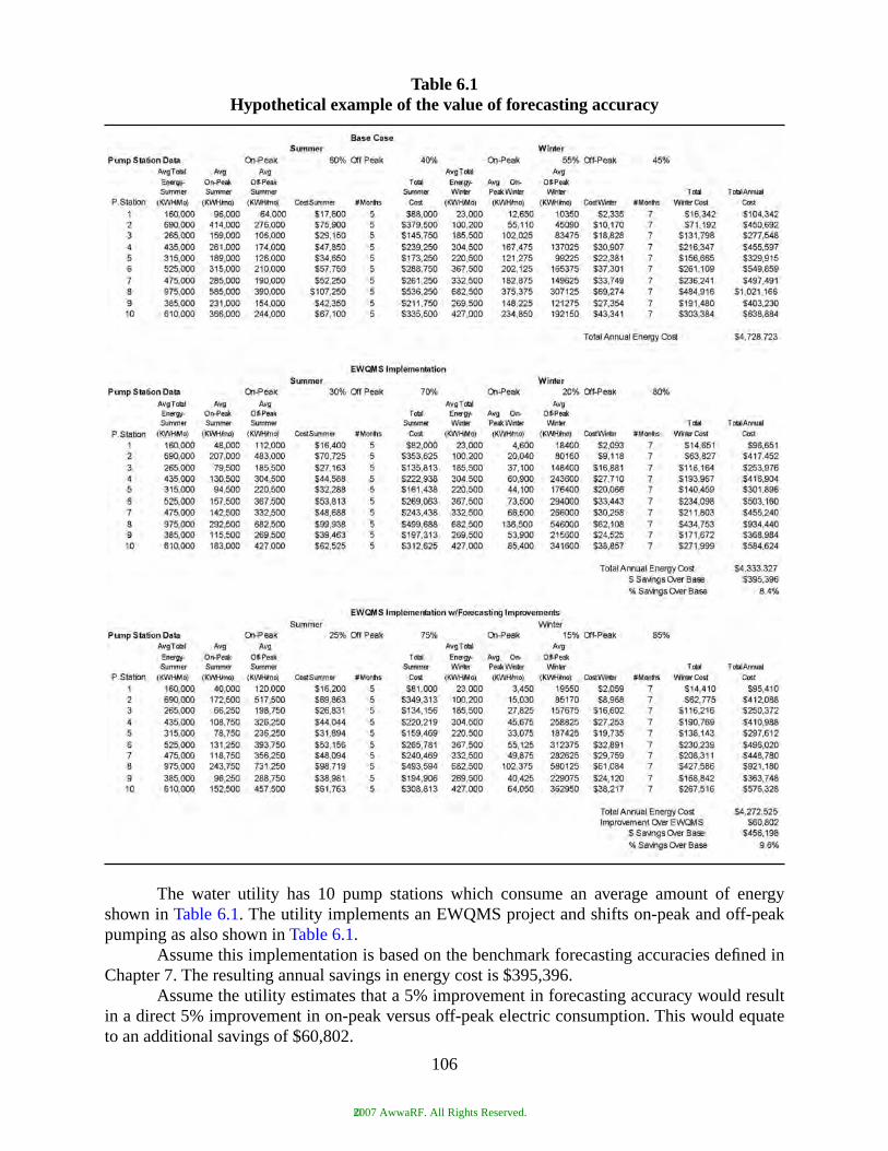
The water utility has 10 pump stations which consume an average amount of energyshown in Table 6.1. The utility implements an EWQMS project and shifts on-peak and off-peakpumping as also shown in Table 6.1.
Assume this implementation is based on the benchmark forecasting accuracies defined inChapter 7. The resulting annual savings in energy cost is $395,396.
Assume the utility estimates that a 5% improvement in forecasting accuracy would resultin a direct 5% improvement in on-peak versus off-peak electric consumption. This would equateto an additional savings of $60,802.
Table 6.1Hypothetical example of the value of forecasting accuracy
106
©2007 AwwaRF. All Rights Reserved.

The utility is receiving a good return on the EWQMS investment. However, the labor costto improve the forecasting accuracy may not be justified from an energy perspective only.
Electric utility hourly forecasting benchmarks are lower than the proposed water utilitybenchmarks in Chapter 7 (3% to 7%). However, the stakes are significantly higher as they relate tothe magnitude of annual cost savings (millions) and system reliability. The high cost to calibrateand maintain the forecasters is justified based on the operational savings.
A similar magnitude of scale can be applied to water utilities. Large water utilities withhigh operating costs may justify accuracy requirements approaching those of electric utilities.However, medium to small water utilities may find the benchmark accuracies proposed in thisreport to be quite acceptable.
107
©2007 AwwaRF. All Rights Reserved.

©2007 AwwaRF. All Rights Reserved.

CHAPTER 7STCF PERFORMANCE CRITERIA, BENCHMARKS, SELECTION
CRITERIA, FUNCTIONAL REQUIREMENTS
PERFORMANCE SUMMARY OF STCF TOOLS
Table 7.1 contains a summary of the results of the Prototype STCF testing.Based on these averages, regression has a slight performance advantage over the Heuristic
and ANN models.Accuracies of the prototypes are slightly better than operational systems. This may be
more a result of the controlled environment of the prototype tests. No effort was made to recali-brate operational STCF models prior to this study.
Table 7.2 is a summary of the results of the Operational Forecasting Systems.
PERFORMANCE BENCHMARKS
The preliminary performance benchmarks set for this study were as follows:
• Hourly AARE less than 10%• Daily ARRE less than 5%
The results of this study exceeded these preliminary benchmarks. However, it should beemphasized that measurements were made under ideal conditions. Extremes in weather condi-tions, such as heavy rains, extended drought, and hurricanes would result in higher forecast errors.
Forecast errors will never be zero and will always be greater than the accumulatedmeasurement and calculation errors. Chapter 6 documents the measures electric utilities take toreduce error rates in their STCF systems. More aggressive, yet achievable, performance bench-marks, for water utilities, may be:
• Hourly AARE less than 7%• Daily AARE less than 4%
SELECTION CRITERIA
Chapter 2 provides a good overview and comparison of STCF methodologies based on theoperational and prototype analysis.
The following are comparisons of the four forecast methods (Heuristic, ANN, SimilarDay, and Regression):
• All tested methods worked well to forecast daily consumption• Daily forecasts improved when hourly data is forecast• ANN model appears to have a better accuracy on an hour-by-hour basis• All of the models require an initial investment of labor to collect and analyze data• ANN models require the least maintenance support• All models share a degradation in performance during seasonal and daily peak periods
109
©2007 AwwaRF. All Rights Reserved.
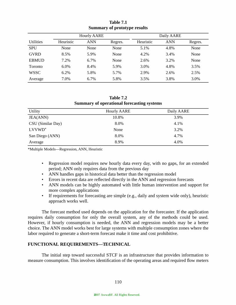
• Regression model requires new hourly data every day, with no gaps, for an extendedperiod; ANN only requires data from the previous day
• ANN handles gaps in historical data better than the regression model• Errors in recent data are reflected directly in the ANN and regression forecasts• ANN models can be highly automated with little human intervention and support for
more complex applications• If requirements for forecasting are simple (e.g., daily and system wide only), heuristic
approach works well.
The forecast method used depends on the application for the forecaster. If the applicationrequires daily consumption for only the overall system, any of the methods could be used.However, if hourly consumption is needed, the ANN and regression models may be a betterchoice. The ANN model works best for large systems with multiple consumption zones where thelabor required to generate a short-term forecast make it time and cost prohibitive.
FUNCTIONAL REQUIREMENTS—TECHNICAL
The initial step toward successful STCF is an infrastructure that provides information tomeasure consumption. This involves identification of the operating areas and required flow meters
Table 7.1Summary of prototype results
Utilities
Hourly AARE Daily AARE
Heuristic ANN Regres. Heuristic ANN Regres.
SPU None None None 5.1% 4.8% None
GVRD 8.5% 5.9% None 4.2% 3.4% None
EBMUD 7.2% 6.7% None 2.6% 3.2% None
Toronto 6.0% 8.4% 5.9% 3.0% 4.8% 3.5%
WSSC 6.2% 5.8% 5.7% 2.9% 2.6% 2.5%
Average 7.0% 6.7% 5.8% 3.5% 3.8% 3.0%
Table 7.2Summary of operational forecasting systems
Utility Hourly AARE Daily AARE
JEA(ANN) 10.8% 3.9%
CSU (Similar Day) 8.0% 4.1%
LVVWD* None 3.2%
San Diego (ANN) 8.0% 4.7%
Average 8.9% 4.0%
*Multiple Models—Regression, ANN, Heuristic
110
©2007 AwwaRF. All Rights Reserved.

and other sensors used to calculate consumption. For applications related to automatic control ofpumping, new instrumentation may be required.
With the appropriate sensors in place, a preventive maintenance program is required tokeep the instrumentation operational and calibrated.
SCADA system data should be frequently reviewed to insure that data are collected andprocessed without loss of precision. Data quality software tools may be required for advancedsystems to detect and correct invalid and missing data in order to ensure the integrity of both real-time and historical consumption data.
If an hourly forecast is used for real-time pump control, a performance monitor is requiredto detect significant deviations between forecast and actual consumption. Either human interven-tion and/or automatic adaptive control software is required to reforecast and reschedule pumpingto minimize energy cost.
The following should be clearly defined in STCF specifications:
• Applications requiring forecast• Accuracy• Resolution—system, number of service areas• Input data-consumption, weather• System Administrator and human forecaster• Optimization Dynamics—daily, hourly• Regeneration—manual, auto• Input/output data format• System interfaces for data transfer
FUNCTIONAL REQUIREMENTS—HUMAN ELEMENT
Mastering the elements of accurate consumption forecasting is an art—especially for theheuristic method.
Consumption forecasting in an operations environment requires human involvement toreview the STCF performance. A staff assignment is required to make adjustments to the forecastbased on changes to the utility system or unforeseen events. This person or persons should alsowork directly with SCADA software personnel to ensure integrity of the database. They shouldalso work with maintenance staff to correct any field instrumentation problems.
Another important task is intelligence gathering. For example, electrical utilities workclosely with large customers to anticipate their needs. Water utilities should establish personalcontacts with their large customers, such as municipalities or industries, to gather advanced infor-mation regarding changes in consumption patterns.
LESSONS LEARNED IN DEVELOPMENT AND CALIBRATION OF STCF SYSTEMS
The following lessons were learned during development and calibration of the prototypeand operational STCF systems:
• Accuracy of the STCF is highly dependent on quality of historical data• It is important to establish consistent standards for storage calculations• Weather factors, other than precipitation, may not be critical to accurate forecasting
111
©2007 AwwaRF. All Rights Reserved.

• ANN models hold up well over time• Retraining an ANN may degrade the model—take care• Training an ANN with a full year of data provides better results than training with only
a single season of data• Daylight Savings Time must be accounted for to ensure data accuracy• Forecast accuracy is limited by accuracy of measurement equipment• A large number of input parameters can make models less responsive and more
difficult to maintain
112
©2007 AwwaRF. All Rights Reserved.

REFERENCES
Coulbeck, B., S. Tennant, and C. Orr. 1985. Development of a Demand Prediction Program forUse in Optimal Control of Water Supply. In Proc. of the 4th International Conference onSystems Engineering, Coventry Lanchester Polytechnic.
Crommelynck, V., C. Duquesne, M. Mercier, and C. Miniussi. (1991). Daily and Hourly WaterConsumption Forecasting Tools Using Neural Networks. Paris, France: Syndicat desEaux d’Ile-de-France.
Jain, A., and L. Ormsbee. 2002. Short-Term Water Demand Forecast Modeling Techniques. Jour-nal AWWA, 94:(7).
Khotanzad, A. 1999. Natural Gas Load Forecasting With Combination of Adaptive Neural Net-works. In Proc. of International Joint Conference on Neural Networks, Washington,D.C., July 10–16, 1999.
Lamb, P., and D. Logue. 2001. Implementation of a Gas Load Forecaster at Williams Gas Pipe-line. Presented at 2001 Pipeline Simulation Interest Group Meeting, Salt Lake City,Utah.
Maidment, D.R. 1986. Hourly Urban Water Use Analysis and Forecasting. Research proposalsubmitted to USGS by the Center for Research in Water Resources, University of Texasat Austin.
Maidment, D.R., S. Miaou, and M. Crawford. 1985. Transfer Function Models of Daily UrbanWater Use. Journal of Water Resources Research, 21(4):425.
Papalexopoulos, A.D., S Hao, and T. Peng. 1994. An Implementation of a Neural Network BasedLoad Forecasting Model for the EMS. IEEE Transactions on Power Systems, 9(4):1956.
Papalexopoulos, A.D., and T. Hesterberg. 1990. A Regression-Based Approach to Short-TermLoad Forecasting. IEEE Transactions on Power Systems, 5(4):1535.
Sugianto, L.F., and X. Lu. (n.d.). Demand Forecasting in the Deregulated Market: A BibliographySurvey. Victoria, Australia: School of Business Systems.
Tsoukalas, L.H., and R. Uhrig. 1997. Fuzzy and Neural Approaches in Engineering. New York:John Wiley and Sons.
113
©2007 AwwaRF. All Rights Reserved.

©2007 AwwaRF. All Rights Reserved.

ABBREVIATIONS
AARE Average Absolute Relative ErrorANN Artificial Neural NetworkAPE Absolute Percentage ErrorAR autoregressionARE Absolute Relative ErrorAwwaRF Awwa Research Foundation
Energy Commission California Energy CommissionCSU Colorado Springs Utilities
EBMUD East Bay Municipal Utility DistrictEMS Energy Management SystemEWQMS Energy and Water Quality Management System
GVRD Greater Vancouver Regional District
ISO Independent System Operator
KWH kilowatt hour
LDF Load Distribution FactorLRA Local Reliability AreaLTCF Long-Term Consumption ForecastLVVWD Las Vegas Valley Water District
MAPE Mean Absolute Percentage ErrorMGD million gallons per dayML million litersMLD million liters per dayMPH miles per hour
OO Operations OptimizationOOS Operations Optimization SystemOPS Operations Planner and Scheduler
PAC Project Advisory CommitteePSI pounds per square inch
RMSE root mean squared error
115
©2007 AwwaRF. All Rights Reserved.

SCADA Supervisory Control and Data Acquisition SDWD San Diego Water DepartmentSE State EstimatorSLF System Load ForecastSTCF Short-Term Consumption Forecaster
UV ultraviolet
WCF Water Consumption ForecasterWDF Water Demand ForecasterWSSC Washington Suburban Sanitary Commission
116
©2007 AwwaRF. All Rights Reserved.


6666 West Quincy AvenueDenver, CO 80235-3098 USAP 303.347.6100www.awwarf.orgemail: [email protected]
Sponsors Research
Develops Knowledge
Promotes Collaboration
1P-3.25C-91189-08/07-NH