water resources impacts of uranium mining in the san juan

University of New MexicoUNM Digital Repository

Civil Engineering ETDs Engineering ETDs

7-12-2014

Water Resources Impacts of Uranium Mining inthe San Juan Basin, New MexicoKent Steinhaus

Follow this and additional works at: https://digitalrepository.unm.edu/ce_etds

This Thesis is brought to you for free and open access by the Engineering ETDs at UNM Digital Repository. It has been accepted for inclusion in CivilEngineering ETDs by an authorized administrator of UNM Digital Repository. For more information, please contact [email protected].

Recommended CitationSteinhaus, Kent. "Water Resources Impacts of Uranium Mining in the San Juan Basin, New Mexico." (2014).https://digitalrepository.unm.edu/ce_etds/96

https://digitalrepository.unm.edu?utm_source=digitalrepository.unm.edu%2Fce_etds%2F96&utm_medium=PDF&utm_campaign=PDFCoverPages

https://digitalrepository.unm.edu/ce_etds?utm_source=digitalrepository.unm.edu%2Fce_etds%2F96&utm_medium=PDF&utm_campaign=PDFCoverPages

https://digitalrepository.unm.edu/eng_etds?utm_source=digitalrepository.unm.edu%2Fce_etds%2F96&utm_medium=PDF&utm_campaign=PDFCoverPages

https://digitalrepository.unm.edu/ce_etds?utm_source=digitalrepository.unm.edu%2Fce_etds%2F96&utm_medium=PDF&utm_campaign=PDFCoverPages

https://digitalrepository.unm.edu/ce_etds/96?utm_source=digitalrepository.unm.edu%2Fce_etds%2F96&utm_medium=PDF&utm_campaign=PDFCoverPages

mailto:[email protected]

Kent Steinhaus Candidate Civil Engineering Department This thesis is approved, and it is acceptable in quality and form for publication: Approved by the Thesis Committee: Dr. Mark Stone , Chairperson Mr. Ryan Morrison Dr. Susan Bogus Dr. Ricardo González-Pinzón

Water Resources Impacts of UraniumMining in the San Juan Basin, New

Mexico

by

Kent Steinhaus

B.S., Civil Engineering, University of New Mexico, 2011

THESIS

Submitted in Partial Fulfillment of the

Requirements for the Degree of

Master of Science

Civil Engineering

The University of New Mexico

Albuquerque, New Mexico

May, 2014

c�2014, Kent Steinhaus

iii

Dedication

I dedicate this thesis to my parents Kurt and Jo Beth Steinhaus who have supported

and encouraged my education for my entire life. For that I am eternally grateful.

My girlfriend Katy Belvin who has put up with my endless rants and random

thoughts and supported me through all of it, thank you so much.

Wes Greenwood who has also encouraged me and supported me with my studies, my

research would not be what it is without his technical support and overall input,

thank you.

Lets not forget and all my fellow researchers, students and others who helped me

along my process of writing this document, thank you.

iv

Acknowledgments

First I must acknowledge My professor Mark Stone who has supported me throughthe majority of my college experience, I appreciate your hard work and patience withme as a developing researcher and student.

I also would like to acknowledge Bruce Thomson who has helped me with theidentification of this thesis topic and his input on the direction my research.

I would also like to acknowledge my colleague Wes Greenwood who has alsoencouraged me and supported me with my studies. My research would not be whatit is without his technical support and overall input.

v

Water Resources Impacts of UraniumMining in the San Juan Basin, New

Mexico

by

Kent Steinhaus

B.S., Civil Engineering, University of New Mexico, 2011

M.S., Civil Engineering, University of New Mexico, 2014

Abstract

The objective of this research was to improve understanding of the groundwater im-

pacts of uranium mining in the San Juan Basin by estimating the volumetric amount

of water removed from the underlying Westwater Canyon member aquifer. This was

achieved by modeling a conceptual mine that is based on the physical character-

istics present near the proposed Roca Honda Mine near Grants, New Mexico. An

analysis of the uncertainty of the physical, situational, and model parameters and

their associated sensitivities was conducted so that an understanding of potential

groundwater withdrawals for uranium mining could be gathered. Uranium mining

in the San Juan Basin, New Mexico, has ranged from being active between the years

of 1950 and 1980, to currently non-existent due to volatility in the price of uranium.

Previous mining in the area has caused detrimental e↵ects to water resources in the

area and future mining activity in the area could have a similar e↵ect. Although

it is well known that mining has and will a↵ect water resources in the San Juan

Basin, there is little knowledge on this subject available. The key findings through

vi

the analysis and understanding of the uncertainty and sensitivity of these aquifer

properties were the probability and the range of the volumes and flow rates that

would be extracted for the conceptual mine. This analysis allows for better decisions

and research to be made about future mining activity.

vii

Contents

List of Figures x

List of Tables xii

1 Introduction 1

1.1 Current State of Knowledge . . . . . . . . . . . . . . . . . . . . . . . 4

1.2 Geology, Hydrology and Resources of The San Juan Basin (Site De-

scription) . . . . . . . . . . . . . . . . . . . . . . . . . . . . . . . . . 5

1.3 History of Mining in the Grants district of the San Juan Basin . . . . 10

2 Research Methods 13

2.1 Conceptual Model Framework . . . . . . . . . . . . . . . . . . . . . . 13

2.2 Groundwater Calculations . . . . . . . . . . . . . . . . . . . . . . . . 15

2.2.1 Model Parameters . . . . . . . . . . . . . . . . . . . . . . . . 18

2.2.2 Uncertainty Analysis . . . . . . . . . . . . . . . . . . . . . . . 20

2.2.3 Sensitivity Analysis Methods . . . . . . . . . . . . . . . . . . 23

viii

Contents

3 Results 24

3.1 Verification of Model . . . . . . . . . . . . . . . . . . . . . . . . . . . 24

3.2 Sensitivity Analysis Results . . . . . . . . . . . . . . . . . . . . . . . 27

3.3 Uncertainty Analysis Results . . . . . . . . . . . . . . . . . . . . . . . 28

4 Discussion 34

5 Conclusion 37

A MATLAB code used for uncertainty analysis 42

B MATLAB code used for sensitivity analysis 48

ix

List of Figures

1.1 Energy Resource Regions in the San Juan Basin [1] . . . . . . . . . 4

1.2 General Geologic Structure of the San Juan Basin including all major

layers (Stone, 1983) . . . . . . . . . . . . . . . . . . . . . . . . . . . 6

1.3 Structural Elements of the San Juan Basin and Adjacent Areas (Kern-

odle, 1996) . . . . . . . . . . . . . . . . . . . . . . . . . . . . . . . . 7

1.4 Roca Honda Mine Permit Area (U.S. Forest Service, 2013) . . . . . 8

2.1 Diagram of Conceptual Uranium Mine Dewatering Well . . . . . . . 14

3.1 Time dependence Parameter Sensitivity . . . . . . . . . . . . . . . . 28

3.2 Distribution of Scenario 1 . . . . . . . . . . . . . . . . . . . . . . . . 29

3.3 Cumulative Distribution Function of Scenario 1 . . . . . . . . . . . . 30

3.4 Cumulative Distribution Function Plots from Scenario 2 . . . . . . . 30

3.5 Distribution of Scenario 3, With T, S, Expansion Rate and Depth of

Drawdown varied . . . . . . . . . . . . . . . . . . . . . . . . . . . . 32

3.6 Cumulative Distribution Function of Scenario 3 . . . . . . . . . . . . 32

x

List of Figures

3.7 Cumulative Distribution Function while holding individual parame-

ters constant . . . . . . . . . . . . . . . . . . . . . . . . . . . . . . . 33

xi

List of Tables

2.1 Modeled parameters used in the Theis Cooper-Jacob Approximation 20

3.1 Parameters Used for 1st Method of Model Verification, data from

Kernodle (1996) and Hydrosceince Associates Inc. (2011) . . . . . . 25

3.2 Historical Pumping Rates from Uranium Mines in the San Juan Basin 26

3.3 Volumes of Water Extracted in m3 and Flow Rates in m3/s from

Sensitivity Analysis . . . . . . . . . . . . . . . . . . . . . . . . . . . 27

3.4 Volume of Water Extracted in m3 for Method 1 & 2 . . . . . . . . . 31

3.5 Final Volume of Water Extracted in m3 for Method 3 . . . . . . . . 33

xii

Chapter 1

Introduction

• General description of the problem

The goal of this research was to improve the understanding of the potential

groundwater resource impacts of uranium mining in the Grants Mineral Belt by

accomplishing the following objectives. First, model a conceptual mine based on

the physical characteristics present at the proposed Roca Honda Mine in the Grants

Mineral Belt, Ambrosia Lake District, by applying the Theis equation. The proposed

mine is located within portions of Sections 9, 10, and 16, Township 13 North, Range

8 West, New Mexico Principal Meridian (figure 1.4). These sections are located

in McKinley County, New Mexico, approximately 3 miles northwest of San Mateo

and 22 miles northeast of Grants, New Mexico [2]. The Theis equation allows for an

aquifer to be simulated so that calculations about the aquifer and well drawdown can

be conducted. Second, quantify the sensitivity of the model parameters within the

area so that future work can be focused towards the most sensitive parameters and

that more accurate quantification of future water resource impacts can be calculated.

Third, explore the uncertainty that is involved in modeling the proposed Roca Honda

Mine site and provide quantified results of groundwater extraction within the ten to

1

Chapter 1. Introduction

ninety percent probabilities of a cumulative distribution so that better decisions can

be made concerning the existing water resource.

There have been previous attempts at quantifying impacts of uranium mining

in the San Juan Basin [1], but there is a noted high degree of uncertainty that is

involved with these calculations. The general uncertainty involved with this research

is both epistemic and aleatory as there is both random variability as well as a lack

of knowledge and understanding [3]. Uncertainty will be discussed in detail later on

in this document. Calculations about potential water resource impacts have been

made at the Roca Honda Mine to fulfill National Pollutant Discharge Elimination

System (NPDES) requirements by Roca Honda Resources Inc. in conjunction with

the United States Forest Service [2]. To study the groundwater impacts of uranium

mining, a model was constructed that simulates how much water a conceptual ura-

nium mine will withdraw from the underlying geologic layer that contains uranium.

The model will be used to estimate the amount of water that must be removed from

underlying aquifers to support mining.

The calculations of groundwater impacts in this study were done using the Theis

equation [4]. The Theis equation relates a discharge, aquifer drawdown, and the

physical properties of the aquifer that a↵ect flow in a transient groundwater system.

It is used in this research to calculate the flow out of a dewatering well for a conven-

tional mine to operate in the San Juan Basin. This equation was used because it is

a simple approximation and can be rapidly applied to the situation where as a more

complex approach would be much more di�cult to manipulate. It can also be noted

that the Theis equation is applied very often to approximate ground water flows in

real situations and is a proven method of approximation [5–7].

The San Juan Basin of New Mexico has yielded the largest amount of uranium

ore mined in the United States and accounts for over 51 percent of the total uranium

mined in the United States since the 1940s [8]. Currently, Wyoming is the largest

2


producer of uranium in the United States [9], but historically the San Juan Basin

generated more than 154 million kilograms (kg) of uranium from the Grants deposits

in New Mexico between 1950 and 2002, and more than 136 million kg of uranium

remains as unmined resources [10]. Although it is speculated that uranium mining

has a↵ected the water quality and the health of the general population in the area

[11], there has been little research focused on the current and future impacts of

uranium mining on water resources in the region. Employment of mining in the state

began in as early as 1950 with a mine operated by the Kerr McGee Oil Company

[12], reaching its peak in 1978, then rapidly declining to almost zero in the 1980s due

to the rapid decline in price for uranium. Currently, coal, copper and potash make

up the majority (80%) of the mining activity in the state [13].

The Grants district, also referred as the Grants Mineral Belt (Figure 1.1) is lo-

cated within the San Juan Basin and is divided up into seven sub-mining districts.

These districts are Ambrosia Lake, Church Rock, Crownpoint, Laguna, Marquez,

Nose Rock, and Smith Lake. There are approximately 115 identified bodies of ura-

nium resource in the San Juan Basin [10]. The mine site studied in this research is

located in the Ambrosia Lake District of the San Juan Basin in the Grants Mineral

Belt. The Ambrosia Lake district is historically the most active district and currently

has the most momentum for renewed uranium-mining activity.

The Roca Honda Mine site was used to quantify the e↵ects of uranium mining

on underground resources in the San Juan Basin because it has a record of aquifer

properties, historical pumping rates, and it is a proposed site for future uranium

mining in New Mexico. Calculations were conducted using the Theis equation (e.g.

[4]) and was compared to a MODFLOW 2005 model developed by Intera [2]. Results

were validated from historical pumping records via the New Mexico Bureau of Mines

and Minerals Resources [1]. These calculations were then conducted via a MATLAB

program to allow evaluation of uncertainty and sensitivity to input parameters.

3


Figure 1.1: Energy Resource Regions in the San Juan Basin [1]

1.1 Current State of Knowledge

Water resources impacts from uranium mining in the San Juan Basin are poorly

understood. The information that is generally relied on regarding the hydrogeologic

properties of the San Juan Basin originate from a groundwater model developed by

Kernodle [14] and aquifer properties defined by [1] in a study by the New Mexico

Mines and Minerals Bureau. Interested mining companies hold information about

aquifers in the San Juan Basin, but this information is not readily available to the

public. Recent attempts at defining the aquifer properties have been focused on

4


the Westwater Canyon Member of the Morrison Formation (described below). Data

has been collected by Roca Honda Mineral Resources Inc. [2] by constructing a test

well and conducting drawdown/recovery tests [15]. This data along with information

from [1, 14] was used by Intera to create a three-dimensional (3D) groundwater model

using MODFLOW 2005. This model was created to study the potential groundwater

impacts of the proposed Roca Honda mine in accordance of meeting environmental

impact study (EIS) requirements.

1.2 Geology, Hydrology and Resources of The San

Juan Basin (Site Description)

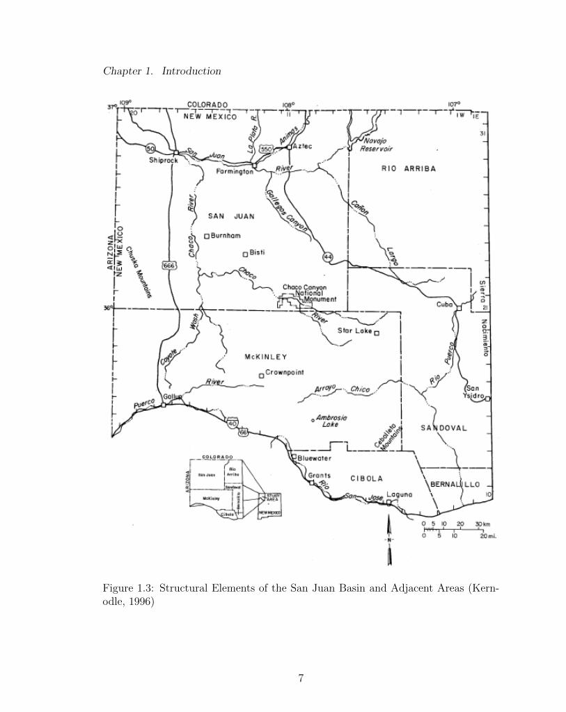
The San Juan Basin is located predominately in New Mexico, but the extent of

the basin extends into Colorado, Arizona, and a small part of Utah (Figure 1.3).

The area of land that it makes up is 54,390 square kilometers. Formed during the

Laramide Orogeny, the San Juan basin consists of layers of sedimentary rock that

date from the Cambrian to Tertiary age [14]. The geology of the San Juan Basin

has been studied mainly from outcroppings and well drilling logs [1]. The general

geologic stratigraphy can be seen in Figures 1.3 & 1.2. There are approximately 17

hydrostratigraphic units that range in elevation from approximately 3,048 m above

sea level to 3,048 m below sea level Figure 1.2.

The conceptual mine that is studied in this report is located near the proposed

Roca Honda Mine. It is located near the town of Grants (NM), and North West

of the Mt. Taylor Mountains Figure 2.1. The permit area encompasses 7.8 km2

within the San Juan Basin. It is under the ownership and maintenance of the Cibola

National Forest.

5


Figure 1.2: General Geologic Structure of the San Juan Basin including all majorlayers (Stone, 1983)

6


Figure 1.3: Structural Elements of the San Juan Basin and Adjacent Areas (Kern-odle, 1996)

7


Figure 1.4: Roca Honda Mine Permit Area (U.S. Forest Service, 2013)

The layer of most interest to this research is the Morrison formation. The Mor-

rison formation is a series of 5 layers, generally consisting of alternating sandstone

aquifers and silt and shale aquitards [1]. The layers of the Morrison in the order

highest elevation to lowest elevation are the Jackpile formation (sandstone, aquifer),

Brushy Basin member (shale, aquitard), Westwater Canyon member (sandstone,

aquifer), Recapture member (shale, aquifer), and Salt Wash member (sandstone,

8


aquifer). The Westwater Canyon member of the Morrison Formation is the most

important geologic layer due to its mineral composition that contains the highest

concentrations of uranium. See Figure 2.1 for a simple schematic of where this mem-

ber is located within the Morrison formation. It mainly consists of Sandstone that is

intermingled with some shale and clay stone, mainly in the northeastern portion of

the San Juan Basin. However, near the Grants Mineral belt the Westwater Canyon

member is known to consist entirely of sandstone.

The hydrology and hydraulic properties of the San Juan Basin’s groundwater

reservoirs are poorly understood although there have been a few studies done on

this regional area hydraulic properties [1, 14]. The systems groundwater resources

can be assumed to be in steady state equilibrium [14] since the inflows of the San

Juan Basin’s groundwater system have been calculated to approximately equal the

outflows [14]. The main source of recharge to the aquifers is through surface water

infiltration through faults and outcroppings of precipitation that is not consumed

through evaporation, sublimation and transpiration [14]. The main sources of out-

flows are the aquifers discharging to streams and arroyos, most of which have dry

beds year-round [2]. Due to these reasons it is estimated that the water budget for

the groundwater resources in the San Juan Basin is Qin �Qout = 0 [2].

The hydraulic properties of the Westwater Canyon member are of much interest

because it contains the highest concentration of uranium and it will need to be de-

watered to extract the uranium resource via under ground mining. These hydraulic

properties are known to be highly variable throughout the extent of the San Juan

Basin [1]. The Westwater Canyon member has been most widely utilized for uranium

mining. A majority of the wells that have been constructed down to the Morrison

formation are used for the sole purpose of dewatering uranium-mine sites, though

some wells in the area are used for domestic and agricultural use. The current

knowledge of the hydraulic properties of this member within the San Juan Basin

9


were determined through a series of drawdown and recovery tests performed on 31

wells in the study area [1]. These hydraulic properties can be found in Table 1 and

are explained later in the methods section. Another study available was done in 2011

and described some limited aquifer properties of the Westwater Canyon member at

the proposed Roca Honda Mine site through a similar drawdown and recovery test

previously done by [1, 15]. These parameters are described in the methods section,

Table 2.1.

1.3 History of Mining in the Grants district of the

San Juan Basin

It was not until the mid 1940s in the United States that uranium was a highly

valuable commodity. This was mainly due to the development of the atomic bomb

in Los Alamos, New Mexico. It was originally believed that uranium ore would

have had to be imported from far away locations such as Africa or Canada [16] but

uranium ore was discovered near Grants and the Haystack Mountain in 1950 [16].

The Ambrosia Lake region was soon to follow in 1955 being only 25 miles northwest

of Grants. This region, as we know it today, has been the largest producing region of

uranium in U.S. history, containing much of the highest-grade uranium ever mined

in the United States.

Uranium production in the San Juan Basin was previously the largest producer

of uranium in the United States. New Mexico alone in 1978 produced 18.3 million kg

of uranium, making up 47 percent of the total uranium mined in the United States

during that time. Production began to decline in 1979 due to a decline in uranium

prices by up to 25% [16]. The lowered uranium prices caused a major decline in

mining activity and by 1987, after the tragedy in Chernobyl, most uranium mining

10


had ceased in the San Juan Basin.

In the San Juan Basin there have been over 200 documented mines in the 7 sub-

districts (McLemore, 2013). Over the 52 years of production of uranium, there have

been over 154 million kg of uranium documented originating from the Grants District

and over 136 million kg remain unmined [10]. These uranium deposits have a range

of concentration ranging from the highest grade (calculated in kg U3O8

kg Soil) 0.5% near

Mt. Taylor to lower than 0.1% in many other parts of the district. The majority of

uranium resources have been mined from the Morrison formation, specifically 1.5*108

kg of uranium has been mined from it [10]. Only 212,281 kg of uranium has been

mined from all other sandstone formations in the Grants District [10].

Presently, uranium prices are still impacted by the disaster at Fukushima, Japan

in 2011 [17]. Uranium prices were on the rise, projected to reach $63.50/kg, but

shortly after the nuclear plant failure prices of uranium dropped to around $18.14/kg.

The volatility of uranium prices has been the most probable reason for no re-

newed uranium mining activity in the San Juan Basin. There has been some in-

terest in renewing mining activity in New Mexico. There are currently seven dif-

ferent companies in the process of assessing and acquiring permits to begin min-

ing. The companies interested in beginning mining include Strathmore Resources

US Ltd. (http://www.strathmoreminerals.com ), Uranium Resources, Inc. (URI;

http://www.uraniumresources.com/), Rio Grande Resources (http://www.ga.com/nuclear-

fuel/rio-grande-resources), Laramide Resources Ltd. (http://www.laramide.com/),

Uranium Energy Corp. (http://www.uraniumenergy.com/), Trans America Indus-

tries Ltd., and Aus American Mining.

Strathmore Resources, although having been recently purchased by Energy Fuels

Inc., is the closest to beginning mining activity and has almost completed the per-

mitting process for a mine in the Ambrosia Lake District near Mt. Taylor. Since

the recent acquisition of the company from Strathmore, Energy Fuels is awaiting

11


approval from the state of New Mexico and is hoping to commence mining activity

in 2016. This area has been identified to contain a large reserve of uranium (7.62

million kg of uranium) at a relatively high grade (0.404%).

12

Chapter 2

Research Methods

2.1 Conceptual Model Framework

An analytical model was constructed that applies the Theis equation’s Cooper Ja-

cob straight-line approximation [4] to quantify the flow rate and volume of water

extracted from a single mine. The conceptual mine was constructed to allow the ex-

traction of ore from the Westwater Canyon formation near the proposed Roca Honda

Mine site by dewatering the aquifer. The Westwater Canyon formation aquifer is a

known confined aquifer that exists between two aquitards, i.e., the Brushy Basin

Member and the Recapture Member. These aquitards are defined to not contribute

any water to the Westwater Canyon formation. To extract the ore, a shaft must be

drilled and the aquifer must be initially dewatered to the radius of the shaft to com-

mence mining. This initial time to sink the shaft and dewater the aquifer is dictated

by numerous factors, and for this model it was assumed to be 2 years so that it can

be compared to the conditions of the proposed Roca Honda Mine. To extract the

ore, horizontal shafts (known as stopes) are blasted, scraped out, and supported by

pillars along the horizontal axis that contains the ore body. The radius of the mine

13

Chapter 2. Research Methods

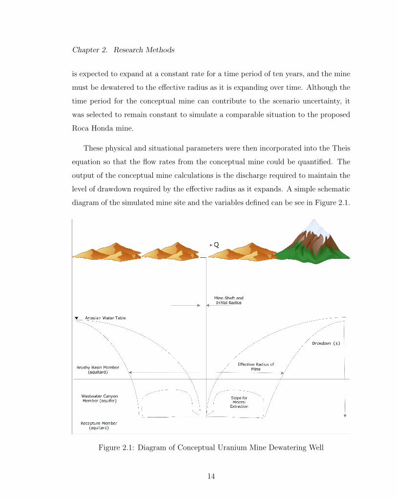
is expected to expand at a constant rate for a time period of ten years, and the mine

must be dewatered to the e↵ective radius as it is expanding over time. Although the

time period for the conceptual mine can contribute to the scenario uncertainty, it

was selected to remain constant to simulate a comparable situation to the proposed

Roca Honda mine.

These physical and situational parameters were then incorporated into the Theis

equation so that the flow rates from the conceptual mine could be quantified. The

output of the conceptual mine calculations is the discharge required to maintain the

level of drawdown required by the e↵ective radius as it expands. A simple schematic

diagram of the simulated mine site and the variables defined can be see in Figure 2.1.

Figure 2.1: Diagram of Conceptual Uranium Mine Dewatering Well

14


The application of the Theis equation to quantify the discharge (Q) and volumet-

ric water withdrawals were employed through MATLAB. The code associated with

these MATLAB calculations can be reviewed in Appendix A and B.

2.2 Groundwater Calculations

To approximate the e↵ects of a conceptual mine near the proposed Roca Honda

Mine, the flow rate required to dewater the Westwater Canyon Member for mining

activity was estimated using the Theis Equation. This method estimates the pump-

ing rates and ultimately volume of water required for mining activity in the Morrison

formation. For the application of the Theis equation, the following assumptions were

made about the conceptual mine and aquifer modeled in this research [4].

• The aquifer is homogeneous, isotropic, of uniform thickness, and of infinite area

extent.

• Before pumping the piezometric surface is horizontal.

• The well is pumped at a constant discharge rate.

• The pumped well penetrates the entire aquifer, and flow is everywhere hori-

zontal within the aquifer to the well.

• The well diameter is infinitesimal so that storage within the well can be ne-

glected.

• Water removed from storage is discharged instantaneously with decline of head.

In reality these assumptions are rarely met although it is accepted by the scientific

community that while all assumptions are not met, the Theis equation can give a

15


good approximation of ground water calculations [5–7]. The Theis equation has

been adapted by other methods of analysis such as the Cooper-Jacob approximation

and Chow Method so that simpler approximations can be readily made in the field

[4].

The Theis equation(equation 2.1) relates a discharge, aquifer drawdown, and the

physical properties of the aquifer that a↵ect flow in a transient groundwater system.

s =Q

4⇡TW (u) (2.1)

Where, Q is the discharge (L3/t), T is the transmissivity (L2/t), pi (unitless) is

equal to 3.14, and W (u) is the well function of u (L), s is equal to the drawdown (L).

u (Eq. 2.2) is referred to as the exponential integral and is determined as follows:

u =r

2S

4Tt(2.2)

Where r is the radius of the well (L), S is the Storage Coe�cient (unitless), and

t is the time since the beginning of pumping. The well function is an exponential

integral as defined in equation 2.3 [4].

W (u) =

Z 1

u

e

�u

u

du = �.5772� ln(u) + u� u

2

2 ⇤ 2! +u

3

3 ⇤ 3! ... (2.3)

The equation used for calculating pumping rates is the Cooper-Jacob straight-

line solution of the Theis equation (Eq. 2.4). Where r is the radius of the mine (L)

and s is the drawdown (L).

Q =4⇡Ts

ln

�2.25Ttr2S

� (2.4)

16


W (u) = ln

✓2.25Tt

r

2S

◆(2.5)

For the Cooper-Jacob approximation, the well function W(u) from Equation 2.1

is replaced in Equation 2.4 (see Equation 2.5) and is allowed so long as u is less than

or equal to 0.01 [4]. For small values of r and large values of t, u is small therefore

making the values after the 2nd term in Equation 2.3 negligible. This is why the

Cooper-Jacob approximation is allowed. The Cooper-Jacob approximation results

in a straight-line relationship between t and s.

For all calculations of flow-rate using equation 2.4 the initial radius of the mine

(r) is 3.1 m and will increase with time as defined in Equation 2.6. To simulate the

conditions of a conceptual uranium mine, the radius of the mine will expand at a

constant rate associated with the time vector t. The expansion rate is defined to

have units of (L/t). The drawdown depth (s) for the conceptual mine is defined as

the depth of water that must be removed measured as the top of the piezometeric

head above the aquifer to the bottom of the aquifer at the edge of the mine radius,

see Equation 2.7. This is to simulate the condition that a dry mine well must be

maintained so that uranium ore can be extracted from the mine.

r = 3.1 + (expansion rate) ⇤ t (2.6)

s = (depth of piezometetric head above aquifer) + (aquifer thickness) (2.7)

The Theis Cooper-Jacob approximation (Eq. 2.4) was used for all of the calcu-

lations of discharge from the conceptual mine in this research. To ensure that these

calculations did not have large errors, the exponential integral u was calculated at

each step to ensure it was less than 0.01.

17


2.2.1 Model Parameters

The parameters used for the analysis of the conceptual mine studied in this research

consist of both physical and situational parameters (T, S, t, s, and r) of Equation 2.4.

How these parameters where used are explained below and are used in both the

uncertainty analysis and the sensitivity analysis. The constant values and ranges in

which the parameters have been analyzed are summarized in Table 2.1.

Transmissivity represents the rate at which water flows horizontally through an

aquifer and is defined in this model in units of meters squared per day. Transmissiv-

ity ranges between values of 0.19 m2/d to 44.6 m2/d within the San Juan Region [1].

From the pumping test performed within the permit area of the Roca Honda Re-

sources (RHR) Mine site, a better understanding of the transmissivity was achieved.

It ranges between the values of 6 m2/d to 11.6 m2/d [15]. The constant value for

transmissivity is 10.6 m2/d this is the median value of transmissivity in the West-

water Canyon member of the San Juan Basin defined in [1]. The transmissivity

parameter was evaluated between both the regional range and the RHR mine site

range to better understand how the spatial variability a↵ects the final water resource

impact.

The storage coe�cient represents the property of the Westwater Canyons Member

to store water. The storage coe�cient ranges between 0.00002 - 0.0002 [1]. Since

Roca Honda Resources defined the value of the storage coe�cient within the Roca

Honda Mine site to be 0.00024 [15], it was used as the constant value for analysis.

Depth of drawdown, measured in meters, represents the drawdown parameter s of

the Cooper-Jacobs approximation of the Theis Equation (Eq. 2.4). The piezometric

head in the Westwater Canyon Member is known to be around 243.8-274.3 m above

the top of the aquifer near the Roca Honda Mine site [2] and the thickness of the

aquifer is known to vary between 30.5 and 121.9 m [1], making the depth of drawdown

18


to range between 274.3-396.2 m. The constant value for aquifer thickness was selected

to be 76.2 m as this was the median value defined by [1] for the Westwater Canyon

member in the San Juan Basin. The constant value of 243.8 m for the piezometric

head of the Westwater Canyon member above the top of the aquifer was chosen

to compare to the proposed Roca Honda mine as this was the value used in the

groundwater impact calculations made by Hydroscience Associates Inc. (2011).

Expansion rate, measured in meters per day, represents the rate at which the ini-

tial mine radius of 3.1 m will expand each day due to mining activity. The expansion

rate can be considered part of the scenario uncertainty that will be explained later.

It is not a known parameter and thus the range of 0.3 to 1.5 m/d was considered.

Other scenario parameters include the time of initial dewatering and time to sink

the mineshaft. These have both been lumped into one parameter so that it can be

compared to the proposed Roca Honda Mine and is set to 2 years. The constant

value of 1.5 m/d was selected for the expansion rate since there were no values to

compare to the situation.

The remaining two situational parameters summarized in Table 2.1, initial dewa-

tering/time to sink shaft, and duration of mining have potential ranges of values that

are not known and were estimated. The constant values were chosen to compare to

the proposed Roca Honda Mine [2].

The model parameter of the time step allows the conceptual model to calculate

the instantaneous volume discharged from the mine during di↵erent times during

the dewatering and mining period. Since the model input of t is the time since the

beginning of pumping the time step would begin with a value of 30 days increasing

by 30 days for each time step until it reaches the end of the mining period at a

maximum value of 4370 days (12 years). The time step of 30 days was chosen so

that calculations could provide a detailed resolution of results.

19


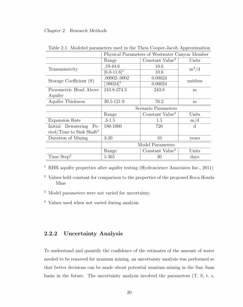
Table 2.1: Modeled parameters used in the Theis Cooper-Jacob Approximation

Physical Parameters of Westwater Canyon MemberRange Constant Value4 Units

Transmissivity.19-44.6 10.6

m2/d[6.0-11.6]1 10.6

Storage Coe�cient (S).00002-.0002 0.00024

unitless[.00024]1 0.00024

Piezometric Head AboveAquifer

243.8-274.3 243.8 m

Aquifer Thickness 30.5-121.9 76.2 m

Scenario ParametersRange Constant Value4 Units

Expansion Rate .3-1.5 1.5 m/dInitial Dewatering Pe-riod/Time to Sink Shaft2

180-1000 720 d

Duration of Mining 3-20 10 years

Model ParametersRange Constant Value4 Units

Time Step3 1-365 30 days

1 RHR aquifer properties after aquifer testing (Hydroscience Associates Inc., 2011)

2 Values held constant for comparison to the properties of the proposed Roca HondaMine

3 Model parameters were not varied for uncertainty.

4 Values used when not varied during analysis

2.2.2 Uncertainty Analysis

To understand and quantify the confidence of the estimates of the amount of water

needed to be removed for uranium mining, an uncertainty analysis was performed so

that better decisions can be made about potential uranium mining in the San Juan

basin in the future. The uncertainty analysis involved the parameters (T, S, t, s,

20


and r) of Equation 2.4. This was conducted to determine which parameters have

the greatest uncertainty, the range in which they vary, and which parameters have

the greatest e↵ect on the flow rate from the dewatering mines and volume of water

extracted from the aquifer.

Since knowledge about the San Juan Basin and its aquifer parameters consist

of empirical data such as observations many of the known ranges of values have an

associated uncertainty. One source of uncertainty comes from the measurement of

these parameters. It exists because there is only one set of data used to determine the

aquifer parameters and this data is limited to only 31 well tests across the entire San

Juan Basin [1]. Another source of uncertainty comes from applying these parameters

as if they were uniform across the entire San Juan basin. In systems this large

and variable, this assumption introduces uncertainty to calculations. In reality it

is understood that these parameters are not uniform and that for each individual

location the properties of the aquifers are di↵erent from site to site.

There are at least three types of uncertainty that are involved with any un-

certainty analysis, parameter, scenario, and model uncertainty [18]. Many of the

physical parameters such as T, S, and aquifer thickness used to quantify the e↵ects

of dewatering a mine for uranium extraction in the San Juan basin are uncertain

because they rely on the limited knowledge about the geology and aquifer properties

of the ore bodies, these are the parameters that have been modeled in this research

to understand the parameter uncertainty. Furthermore, there is general uncertainty

about future mining activity in the area such as expansion rate of the mine, time

it will take to sink the mineshaft, and the duration that mining activity will oc-

cur. These are the parameters that contribute to the scenario uncertainty. Since the

proposed Roca Honda Mine has been used to define some of these scenario parame-

ters [2], the only scenario parameter that was studied for uncertainty in this research

is the expansion rate. Finally, there is general uncertainty involved in how the model

21


is constructed. It must be noted that a model that simulates a conceptual uranium

mine can be constructed in many di↵erent ways and that parameters such as the

length of the time step or the modeling program that the conceptual model was cal-

culated in can inevitably a↵ect the final outcome and can contribute to uncertainty.

No model uncertainty was modeled in this research, but it could be incorporated in

future work.

The calculations for uncertainty were performed using the Theis Cooper-Jacob

approximation through a MATLAB code that allowed for multiple simulations of

various configurations of parameters. This MATLAB code simulated the mining

conditions of the proposed Roca Honda Mine by using the parameters defined in Ta-

ble 2.1. The MATLAB code allowed the transmissivity, storage coe�cient, depth of

drawdown, and expansion rate parameters to vary randomly for each iteration within

its range of known values. It was assumed that all values of input parameters are

equally likely (uniform distribution) unless it was defined as a constant value, since

the information about the spatial variability of these values was not known. With

more information about how these parameters vary throughout the San Juan Basin,

di↵erent types of distributions for the physical parameters could be selected. 100,000

iterations of the model were performed for each variation of the model described be-

low. The output of the model at each iteration was a total volume extracted for the

12 year simulation period.

To better understand how the parameters that had a variable range of values

and did not have a single constant value defined in Table 2.1 (transmissivity, storage

coe�cient, depth of drawdown, and expansion rate) it was studied how they a↵ected

the uncertainty of the total volume extracted from the conceptual mine. Three

di↵erent scenarios were used to evaluate this uncertainty. The first scenario (scenario

1) studied allowed all of the parameters to be varied randomly between their value

ranges with a uniform distribution. The second scenario (scenario 2) allowed each

22


parameter to be held constant while the others varied randomly so that the e↵ect

each parameter on the uncertainty analysis could be studied. Finally, scenarios one

and two were performed in the same fashion while using the transmissivity values

defined by RHR’s pump test (Table 2.1) so that the e↵ect of the spatial variability

of this parameter could be studied (scenario 3).

2.2.3 Sensitivity Analysis Methods

The parameters used to calculate the flow rate and final volume of water removed

from the Westwater Canyon Member for uranium mining are known to exist over

a range of values within the San Juan Basin, see Table 2.1 [1, 15]. By varying

each parameter within its known range while holding the other parameter values

constant, the sensitivity of the resultant flow rate and total volume removed can

be better understood. The parameters that were varied are transmissivity, storage

coe�cient, depth of drawdown, and expansion rate.

The sensitivity analysis was performed by calculating the groundwater flow rate

required for extracting uranium at the proposed Roca Honda Mine over a 12-year

time period. The conceptual model described earlier was used for this calculation

by holding all of the parameters at their constant value (Table 2.1) while allowing

one parameter vary across its range of values describes in Table 2.1. The parameters

that where studied for sensitivity are transmissivity, storage coe�cient, depth of

drawdown, and expansion rate. This allowed for a better understanding of how each

parameter a↵ected the flow rate.

23

Chapter 3

Results

3.1 Verification of Model

Two methods were used to verify the results of the analytical model. For both

methods, the historical data from the NM Bureau of Mine & Minerals Resources

(NMBMMR) [1] were used to compare observed flow rates to modeled flow rates

(Table 3.2). The first way the model was verified was through a single run of the

analytical model with a time vector of 12 years using the aquifer parameters that

are determined by [1] as median values in the Morrison formation. Since these are

accepted values for the aquifer parameters of the Morrison formation that is why

they were used as the criterion of the Morrison aquifer during the first validation

method. The parameters used in the first verification method can be seen in Table

3.1. The resulting flow rate from the model is 10.98 m3/s and is only about 10%

di↵erent from the historical flow rates reported for mining in the Ambrosia Lake

District (Table 3.2). This serves to verify that the method used in this analysis is a

reasonable approximation.

The second way that the results of this model was verified is by comparing the

24

Chapter 3. Results

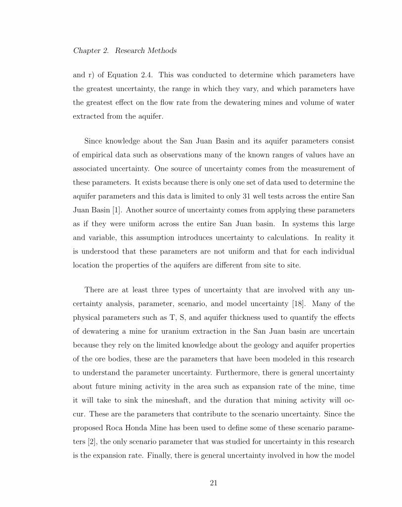
Table 3.1: Parameters Used for 1st Method of Model Verification, data from Kernodle(1996) and Hydrosceince Associates Inc. (2011)

Parameters Used forCalibration

Kernodle Median Value RHR Pump Test Units

Transmissivity 14.4 6.0-11.6 m2/dStorage Coe�cient 2.0*10�4 2.4*10�4 unitlessDepth of Water TableAbove Aquifer

243.8 N/A m

Thickness of Westwa-ter Canyon Formation

76.2 Approx 122 m

median of the total volume removed from the aquifer for the uncertainty analysis

(100,000 iterations) to historical values. The median volume from this analysis is

6.07*107 m3. This volume, when averaged over 12 years, equates to a flow rate of 9.6

m3/min. It can be seen in Table 3.2 that this flow rate is only 1.5% di↵erent from

the historical values reported for mining the Ambrosia Lake District (Table 3.2) and

serves to verify that the method used in this analysis is a reasonable approximation.

Previous attempts of validating the parameters used by [14] have been made by

Roca Honda Resources (RHR). A test well was installed in the area near the proposed

Roca Honda Mine that provides some limited data on the hydraulic properties of

the Westwater Canyon member. The data about the hydraulic properties from the

Westwater Canyon Member collected by the test well can be seen in Table 2.1, [15].

Since the aquifer parameters reported by RHR lies within the reported hydraulic

parameter range reported by [1], the parameters used for the Roca Honda mine

permit site can be considered validated as well.

25

Chapter 3. Results

Table 3.2: Historical Pumping Rates from Uranium Mines in the San Juan Basin

Location ofMine

Quantitypumped(m3/min)

Quantity dis-charged to streams(m3/min)

Other

Ambrosia Lake area

14.10.22

9.46 1.13-1.898.33 m3/min is used in millprocess. Some is recirculatedfor stope leaching.

14.09.3314.09.3014.09.2414.09.1714.09.3014.09.19

14.09.35 6.06 0 Water diverted for irrigationof rangeland14.09.36 6.06 0

14.09.28 1.32-1.51 0 Most water is recirculated forstope leaching14.09.34 1.32 0

14.10.257.57 2.46

4.54-4.92 m3/min used forstope leaching

14.10.2314.10.32

13.08.07 3.79 3.79Entire discharge diverted forirrigation and stock wateringduring summer months.

Church Rock area

17.16.35 4.73-5.30 0.19 Most water used in mill pro-cess17.16.35 14.20-15.14 14.20-15.14

Smith Lake area

15.14.12 .76-1.14 Intermittent

San Mateo area

13.08.24 18.81-19.00 18.81-19.00

Water provided from shaftand wells. Most of water di-verted for irrigation and stockwater

Laguna-Marquez area

11.04.19 .08-.19 0

Water produced from shaft

11.05.13 0.09 011.05.04 0.57 011.04.19 0.09 011.05.25 4.54 4.5411.03.18 1.89 1.89

Crownpoint area

19.11.31 4.77-5.30 4.77-5.30Water produced from shaftand wells during shaft con-struction

26

Chapter 3. Results

3.2 Sensitivity Analysis Results

The results of this analysis can be seen in Figure 3.1 and Table 3.3. Each indi-

vidual parameter was varied between the ranges specified in Table 2.1, while the

other parameters were held constant, also specified in Table 2.1. By performing the

conceptual model within the specified parameters ranges, a range of resultant flow

rates and volumes of water removed from the Westwater Canyon member for ura-

nium mining from a conceptual mine was determined. This will help to give a better

understanding of how much each individual parameter can a↵ect the final volume of

groundwater extracted.

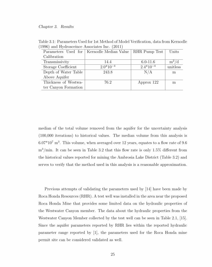
The results of the sensitivity analysis are presented in Figure 3.1 as well as Table

3.3 so that a comparison of how each parameter a↵ects the flow rate and total

volume extracted to its minimum, and maximum value within its specified range

can be determined. One note about Figure 3.1 is that the scenario for the max

storage coe�cient and max expansion rate coincidentally had the same parameters.

This is why they have the same values in Figure 3.1. The ”Transmissivity RHR” in

the legend of Figure 3.1 corresponds to holding the transmissivity parameter values

between what was determined during the pump test performed on the Roca Honda

Mine permit site, (6.0-11.6 m2/d).

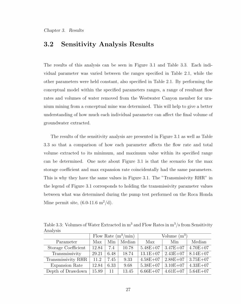
Table 3.3: Volumes of Water Extracted in m3 and Flow Rates in m3/s from SensitivityAnalysis

Flow Rate (m3/min) Volume (m3)Parameter Max Min Median Max Min Median

Storage Coe�cient 12.84 7.4 10.78 5.48E+07 3.47E+07 4.70E+07Transmissivity 29.21 6.48 18.74 13.1E+07 2.43E+07 8.14E+07

Transmissivity RHR 11.2 7.45 9.33 4.58E+07 2.88E+07 3.75E+07Expansion Rate 12.84 6.33 9.68 5.38E+07 3.10E+07 4.33E+07

Depth of Drawdown 15.89 11 13.45 6.66E+07 4.61E+07 5.64E+07

27

Chapter 3. Results

Figure 3.1: Time dependence Parameter Sensitivity

It can be seen in Figure 3.1 that when the transmissivity values were allowed to

range between what is accepted within the entire San Juan Basin, the values of flow

rates are the largest compared to the other flow rates. Once this range is reduced

to the RHR permit site where there is a better understanding of what parameter

values truly exist, transmissivity no longer causes the greatest increase to flow rate

in the model. Once transmissivity is less variable, the parameters of the model are

approximately equally sensitive to their known or estimated ranges.

3.3 Uncertainty Analysis Results

The following figures 3.3, 3.4, 3.6, 3.7, 3.2, 3.5 and tables 3.4 and 3.5 summarize the

output from the three uncertainty scenarios defined in the methods section. Results

are presented graphically in three ways. The first method is presented through a

histogram that plots the number times the resultant volume occurs for each iteration

of the 100,000 iterations versus the resultant volume extracted from the conceptual

28

Chapter 3. Results

mine over 12 years (Figures 3.3 and 3.2). This allows the reader to determine the

distribution of volumes extracted for each scenario. Figures 3.3, 3.4, 3.6 and 3.7

present Cumulative Distribution Function (CDF) graphs that allow the reader to

quickly gather information about each scenario’s modeled volume of water extracted

by displaying the probabilities during the 100,000 simulations performed for analysis.

Finally, this information is summarized in Tables 3.4 and 3.5 for quick comparisons

among the scenarios modeled.

It was found that for scenario 1 the total volume of water extracted during the

12-year simulation had a broader distribution (Figure 3.3) than other scenarios. The

values for the final water extracted between the 10% and 90% probabilities (Figure

3.2) were 2.53*107 m3 and 9.91*107 m3 (Table 3.4). The results of what type of

statistical distribution this result produces was not explored although future work

could be focused on the relevance of the distribution for better understanding the

results.

Figure 3.2: Distribution of Scenario 1

29

Chapter 3. Results

Figure 3.3: Cumulative Distribution Function of Scenario 1

Figure 3.4: Cumulative Distribution Function Plots from Scenario 2

In scenario 2 the result of holding each parameter constant that was previously

allowed to vary randomly in scenario 1 made for a better understanding of which

parameter contributed the greatest amount of uncertainty. When Figures 3.3 and

30

Chapter 3. Results

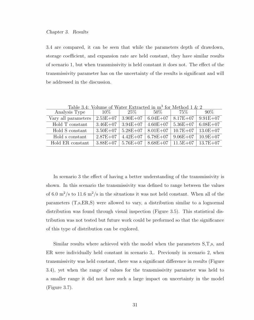
3.4 are compared, it can be seen that while the parameters depth of drawdown,

storage coe�cient, and expansion rate are held constant, they have similar results

of scenario 1, but when transmissivity is held constant it does not. The e↵ect of the

transmissivity parameter has on the uncertainty of the results is significant and will

be addressed in the discussion.

Table 3.4: Volume of Water Extracted in m3 for Method 1 & 2Analysis Type 10% 25% 50% 75% 90%

Vary all parameters 2.53E+07 3.90E+07 6.04E+07 8.17E+07 9.91E+07Hold T constant 3.46E+07 3.94E+07 4.60E+07 5.36E+07 6.08E+07Hold S constant 3.50E+07 5.28E+07 8.01E+07 10.7E+07 13.0E+07Hold s constant 2.87E+07 4.42E+07 6.78E+07 9.06E+07 10.9E+07

Hold ER constant 3.88E+07 5.76E+07 8.68E+07 11.5E+07 13.7E+07

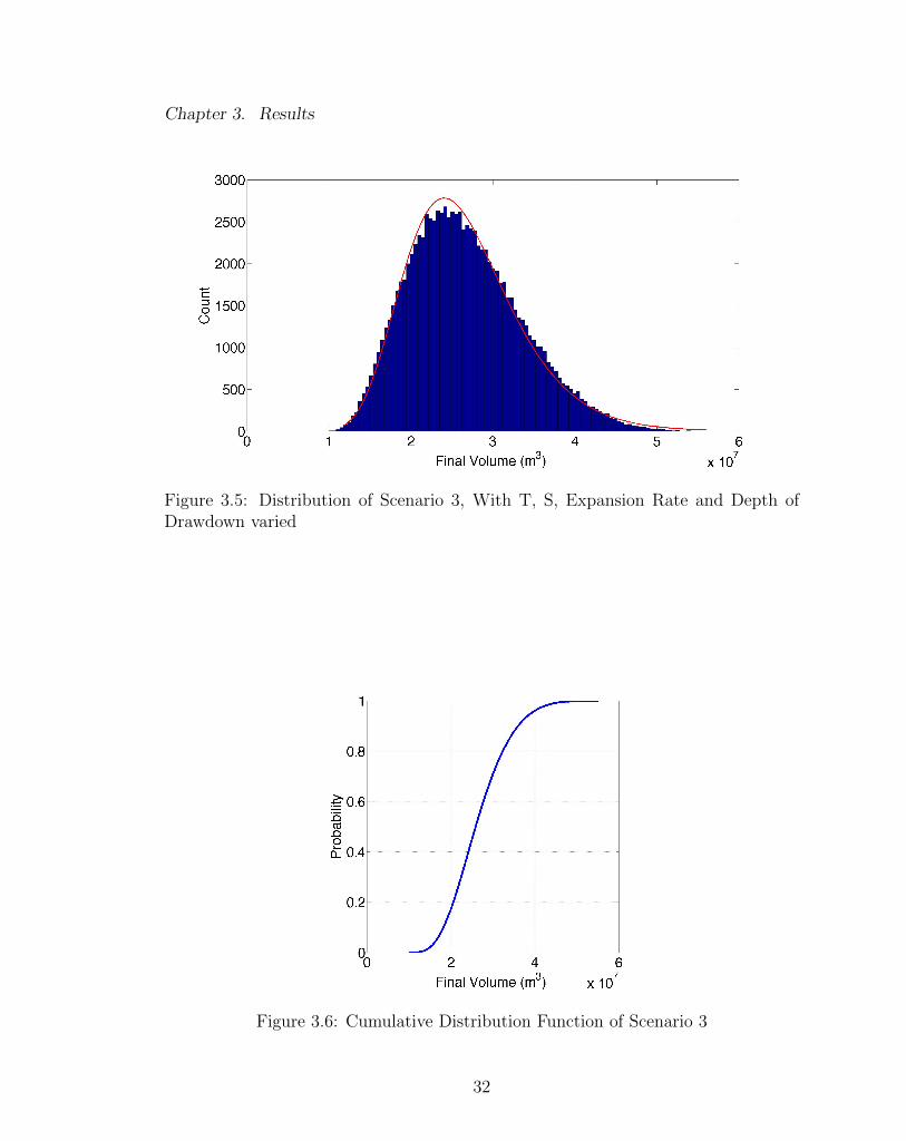
In scenario 3 the e↵ect of having a better understanding of the transmissivity is

shown. In this scenario the transmissivity was defined to range between the values

of 6.0 m2/s to 11.6 m2/s in the situations it was not held constant. When all of the

parameters (T,s,ER,S) were allowed to vary, a distribution similar to a lognormal

distribution was found through visual inspection (Figure 3.5). This statistical dis-

tribution was not tested but future work could be preformed so that the significance

of this type of distribution can be explored.

Similar results where achieved with the model when the parameters S,T,s, and

ER were individually held constant in scenario 3,. Previously in scenario 2, when

transmissivity was held constant, there was a significant di↵erence in results (Figure

3.4), yet when the range of values for the transmissivity parameter was held to

a smaller range it did not have such a large impact on uncertainty in the model

(Figure 3.7).

31

Chapter 3. Results

Figure 3.5: Distribution of Scenario 3, With T, S, Expansion Rate and Depth ofDrawdown varied

Figure 3.6: Cumulative Distribution Function of Scenario 3

32

Chapter 3. Results

Figure 3.7: Cumulative Distribution Function while holding individual parametersconstant

Table 3.5: Final Volume of Water Extracted in m3 for Method 3Analysis Type 10% 25% 50% 75% 90%

Vary all parameters 1.82E+07 2.15E+07 2.59E+07 3.10E+07 3.60E+07Hold T constant 2.09E+07 2.46E+07 2.95E+07 3.52E+07 4.08E+07Hold S constant 3.46E+07 3.95E+07 4.60E+07 5.36E+07 6.08E+07Hold s constant 2.49E+07 2.98E+07 3.62E+07 4.33E+07 5.00E+07

Hold ER constant 2.91E+07 3.39E+07 4.01E+07 4.66E+07 5.28E+07

33

Chapter 4

Discussion

The goal of this research was to improve our understanding of the future groundwater

resource withdrawals of potential uranium mining in the San Juan Basin. For this,

a conceptual mine was modeled using the Theis equation, whose parameters were

informed from the physical characteristics present at the proposed Roca Honda Mine

in the Grants Mineral Belt, Ambrosia Lake District. This research quantified the

sensitivity of the model parameters within the area so that future work can be focused

towards the most sensitive parameters and that more accurate quantification of future

water resource impacts can be calculated. This research explored the uncertainty

that is involved in modeling this situation and provided quantified results within

confidence bounds so that better decisions can be made concerning the existing

water resource.

The sensitivity of the parameters that was calculated in this research provided

flow rates and volumes of potential water extracted for uranium mining. Transmis-

sivity, among the other parameters evaluated for its sensitivity had the largest range

of flow rates and volumes. This parameter has long been known to cause the most

variance in groundwater impact. Since it is understood that this parameter is not

34

Chapter 4. Discussion

well defined, the estimates of groundwater flow rates tend to use conservatively high

values of groundwater pumping for uranium mining [2]. Each parameter such as the

situational rate at which a mine will expand, storage coe�cient, and depth of the

water table each individually have enough uncertainty about what flow rates and

volumes a potential uranium mine could extract. When combined together, they

have similar if not greater impacts on calculations than the transmissivity alone.

Since the majority of previous research about the groundwater impacts of ura-

nium mining use parameters that are part of a spatial area that covers the entire

54,390 km2 of the San Juan Basin, parameters such as transmissivity have a large

range of values. The parameter that contributes the greatest amount of sensitivity

and uncertainty in the analysis of this model is the transmissivity parameter. This

can be seen in both the sensitivity results and the uncertainty results (Tables 3.4

and 3.5, Figures 3.2-3.5). When this value is more tightly bound to a spatial area of

7.8 km2, like in the case of the Roca Honda Resources pump test of the permit site

[15], the results are more constrained (Table 3.5, Figures 3.5,3.6,3.7.

Being that this is one of the first attempts at calculating flow rates from ura-

nium mining dewatering wells the distributions of the inputs of physical, model, and

scenario parameters in the model was not known. Since there was no information

about the distributions of the parameters used in this research, the distribution was

selected to be a uniform distribution. Gathering more information about these pa-

rameters could allow for a most customized distribution and allow for a comparison

of what di↵erent distributions can do to a↵ect the resulting ground water impacts.

The uncertainty analysis provides a range of values that serves to allow for better

decisions to be made about groundwater pumping for underground uranium min-

ing. The uncertainty analysis allows the reader to understand that there are many

potential impacts that uranium mining in the San Juan Basin can cause to ground-

water resources. For example, it is interesting to note that from the results of the

35

Chapter 4. Discussion

uncertainty analysis, the calculated flow rates were on average below the current

projections that Roca Honda Resources have published in the DEIS report for the

proposed Roca Honda mine. The volume of 9.18*107 m3 was one of the highest re-

sults that this particular model calculated, and it was the singular value that RHR’s

used as the groundwater impact over a modeled 12 year mining period. It is not

known what range of values RHR’s model calculated when modeling dewatering for

the mine but it can be assumed they experienced a similar distribution of flow rates

and volumes of water extracted for uranium mining, similar to what was calculated

in this report. It can be seen in the results of the uncertainty analysis that a large

range of calculated final volumes and flow rates imply that these calculations are

uncertain.

36

Chapter 5

Conclusion

The results from the conceptual mine based on the proposed Roca Honda Mine

incorporated the Theis Method Cooper Jacob Approximation and can be considered

a reasonable result although the technique of modeling is simple. The advantage of

using this simple technique allowed for a greater range of possibilities to be studied

in a shorter period of time versus other modeling techniques such as Modflow 2005

among other groundwater modeling programs. Future work could be conducted to

more thoroughly understand the model uncertainty by modeling the same situation

and parameters with di↵erent modeling programs or equations.

The goal of this research was to increase the knowledge about the groundwater

impacts of uranium mining in the San Juan Basin. One of the ways this research

can be useful is that it provides a range of quantified results within calculated prob-

abilities where other studies do not. This can also be useful as a comparison to an

environmental impact statement (EIS) provided by a mining company. This EIS

could have a di↵erent method for calculating groundwater impacts that do not take

into account or recognize that the parameters they are using are uncertain for the

associated calculations. Another way this research can be useful is that it provides

37

Chapter 5. Conclusion

a better understanding of what volumes and flow rates can be expected from poten-

tial uranium mines in the San Juan Basin. With this information provided in this

research better understanding of groundwater impacts of uranium mining in the San

Juan basin and can be used to make better decisions about future mining activity

in the area.

38

References

[1] William Jay Stone et al. Hydrogeology and water resources of San Juan Basin,

New Mexico. New Mexico Bureau of Mines and Mineral Resources, 1983.

[2] Draft environmental impact statement for Roca Honda Mine : Sections 9, 10

and 16, Township 13 North, Range 8 West, New Mexico Principal Meridian,

Cibola National Forest, McKinley and Cibola Counties, New Mexico. MB-R3:

03-25. [Albuquerque, N.M.] : United States Department of Agriculture, Forest

Service, Southwestern Region, [2013], 2013.

[3] Keith Beven and Peter Young. A guide to good practice in modeling semantics

for authors and referees. Water Resources Research, 49(8):5092–5098, 2013.

[4] K Tood and L. Mays. Groundwater Hydrology, volume 3. Wiley, John and Sons,

Incorporated, 2004.

[5] John G Ferris, D B Knowles, RH Brown, and Robert William Stallman. Theory

of aquifer tests. US Government Printing O�ce, 1962.

[6] RN Singh and AS Atkins. Analytical techniques for the estimation of mine

water inflow. International Journal of Mining Engineering, 3(1):65–77, 1985.

[7] R. Singh and A. Atkins. Application of analytical solutions to simulate some

mine inflow problems in underground coal mining. International Journal of

Mine Water, 3(4):1, 1984.

39

REFERENCES

[8] William L Chenoweth. 7. history-uranium mining in the morrison formation.

Modern Geology, 23(1):427–440, 1998.

[9] U.S. Energy Information Administration. 2012 domestic uranium production

report. Technical report, U.S. Department of Energy, 2013.

[10] V. T. McLemore. Uranium resources in the grants uranium district , new mexico

: An update. In New Mexico Geological Society Guidebook, 64th Field Confer-

ence, pages 113–122, 2013.

[11] Robert F Kaufmann, Gregory G Eadie, and Charles R Russell. E↵ects of ura-

nium mining and milling on ground water in the grants mineral belt, new mexico.

Ground Water, 14(5):296–308, 1976.

[12] PA Longmire, BM Thomson, and DG Brookins. Uranium industry impacts on

groundwater in New Mexico, pages 167–183. Number 7. NM Bureau of Mines

and Mineral Resources, Soccoro, NM, 1984.

[13] Virginia T McLemore, Gretchen K Ho↵man, and J Pfeil. Minerals industry in

new mexico in 1998–2000. New Mexico Geology, 24(1):19–28, 2002.

[14] John Michael Kernodle. Hydrogeology and steady-state simulation of ground-

water flow in the San Juan Basin, New Mexico, Colorado, Arizona, and Utah.

US Department of the Interior, US Geological Survey, 1996.

[15] Roca Honda Resources Inc. Baseline data report for the roca honda mine: Rhr

report submitted to new mexico mining and minerals division and u.s. forest

service. Technical report, Cibola National Forest, 2011.

[16] Bureau of Indian A�ars. Uranium development in the San Juan Basin region :

a report on environmental issues : [final report] / prepared by San Juan Basin

Regional Uranium Study, O�ce of Trust Responsibilities, Bureau of Indian Af-

fairs, lead agency. Albuquerque, N.M. : The Study, [1980], 1980.

40

REFERENCES

[17] Jim Green. Uranium flashpoint in wa. Chain Reaction, 115:24, 2012.

[18] Philip D Meyer, Ming Ye, Mark L Rockhold, Shlomo P Neuman, and Kirk J

Cantrell. Combined estimation of hydrogeologic conceptual model, parameter,

and scenario uncertainty with application to uranium transport at the hanford

site 300 area. Technical report, Pacific Northwest National Laboratory (PNNL),

Richland, WA (US), 2007.

[19] V.T. McLemore. New mexico mines database. Mining Engineering, 57(2):42–49,

2005.

[20] Glenn A. Hearne. Evaluation of a potential well field near Church Rock as a

water supply for Gallup, New Mexico / by Glenn A. Hearne. Water-resources

investigations ; 77-98. [Albuquerque, N.M.] : Dept. of the Interior, Geological

Survey, Water Resources Division [New Mexico District], 1977., 1977.

41

Appendix A

MATLAB code used for

uncertainty analysis

• Setting Initial Parameters

• Depth of Draw down uncertainty analysis

clc; clear all; close all

tic

ploti = 1;

fig_size = get(0,’Screensize’);

% Note about code: this code parametriclly varies all but one of the

% following parameters: the depth of drawdown, storage coefficient,

% the transmissivity or the expansion rate. Meanwhile the 4th parameter

% is held constant. The constant values and the parametric ranges are

% stated here:

% % Constant Paramters

42

Appendix A. MATLAB code used for uncertainty analysis

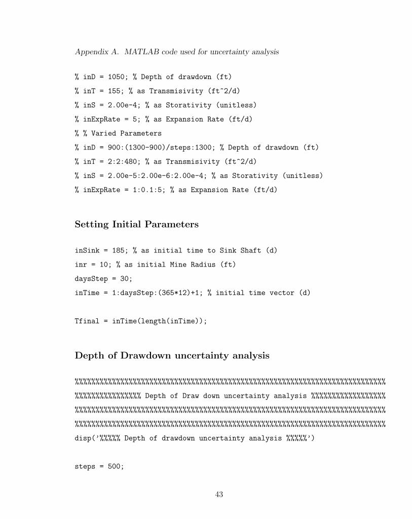
% inD = 1050; % Depth of drawdown (ft)

% inT = 155; % as Transmisivity (ft^2/d)

% inS = 2.00e-4; % as Storativity (unitless)

% inExpRate = 5; % as Expansion Rate (ft/d)

% % Varied Parameters

% inD = 900:(1300-900)/steps:1300; % Depth of drawdown (ft)

% inT = 2:2:480; % as Transmisivity (ft^2/d)

% inS = 2.00e-5:2.00e-6:2.00e-4; % as Storativity (unitless)

% inExpRate = 1:0.1:5; % as Expansion Rate (ft/d)

Setting Initial Parameters

inSink = 185; % as initial time to Sink Shaft (d)

inr = 10; % as initial Mine Radius (ft)

daysStep = 30;

inTime = 1:daysStep:(365*12)+1; % initial time vector (d)

Tfinal = inTime(length(inTime));

Depth of Drawdown uncertainty analysis

%%%%%%%%%%%%%%%%%%%%%%%%%%%%%%%%%%%%%%%%%%%%%%%%%%%%%%%%%%%%%%%%%%%%%%%%%%%

%%%%%%%%%%%%%%%% Depth of Draw down uncertainty analysis %%%%%%%%%%%%%%%%%%

%%%%%%%%%%%%%%%%%%%%%%%%%%%%%%%%%%%%%%%%%%%%%%%%%%%%%%%%%%%%%%%%%%%%%%%%%%%

%%%%%%%%%%%%%%%%%%%%%%%%%%%%%%%%%%%%%%%%%%%%%%%%%%%%%%%%%%%%%%%%%%%%%%%%%%%

disp(’%%%%% Depth of drawdown uncertainty analysis %%%%%’)

steps = 500;

43


calcs = 100000;

% Constant Paramters

inD = 1050; % Depth of drawdown (ft)




% Varied Parameters

% inDrange = 900:(1300-900)/steps:1300; % Depth of drawdown (ft)

inTrange = 50:(480-50)/steps:480; % as Transmisivity in San Juan Basin (ft^2/d)

% inTrange = 65:(125-65)/steps:125; % as Transmisivity in RHR Site (ft^2/d)

inSrange = 2.00e-5:(2.00e-4 - 2.00e-5)/steps:2.00e-4; % as Storativity (unitless)

inExpRaterange = 1:(5-1)/steps:5; % as Expansion Rate (ft/d)

Vfinal = zeros(1,calcs);

for j = 1:calcs

% locRand = round(steps*rand(1)) + 1; % random location in vector

% inD = inDrange( locRand );

locRand = round(steps*rand(1)) + 1; % random location in vector

inT = inTrange( locRand );


inS = inSrange( locRand );


inExpRate = inExpRaterange( locRand );

% Calculate Initial Q

outQinitial = (inT*inD) ...

./( 0.183*log10((2.25*inT*inSink)./(inr^2*inS)) ); % Initial Q (ft^3/d)

% outQinitialCFS = outQinitial/86400; % Converting Q to CFS

44


% Calculate Volume of Water up to Sink Date

outVsink = outQinitial*inSink;

% Cacluating Q for Each Time

outQvector = zeros(length(inTime));

% outQvectorCFS = zeros(length(inTime));

outVvector = zeros(length(inTime));

outVDiffvector = zeros(length(inTime));

for i=1:length(inTime)

currentDay = inTime(i);

if currentDay < inSink

% Radius at this point

mineRadius = inr;

% Q at this point

outQvector(i) = outQinitial;

% outQvectorCFS(i) = outQinitialCFS;

% Volume removed at this point

currentVadd = 0;

outVDiffvector(i) = outQinitial * ( inTime(2) - inTime(1) );

outVvector(i) = outQinitial * inTime(i);

else


dayDiff = currentDay - inSink;

mineRadius = inr + dayDiff*inExpRate;

45


% Q at this point

outQvector(i) = (inD*inT) ...

/( 0.183*log10((2.25*inT*currentDay)/(mineRadius^2*inS)) ); % Initial Q (ft^3/d)

% outQvectorCFS(i) = outQvector(i)/86400; % Converting Q to CFS


% currentVadd = outVsink;

outVDiffvector(i) = outQvector(i) * ( inTime(i) - inTime(i-1) );

outVvector(i) = outVvector(i-1) + outQvector(i) * ( inTime(i) - inTime(i-1) );

end

% outVvector(i) = outVvector(i) + currentVadd;

end

Vfinal(j) = outVvector(length(outVvector));

end

% convert units: 1ft^3 = 2.29568411e-5 acre feet

% Vfinal = Vfinal*(2.29568411e-5);

% convert to metric units: 1ft^3 = 2.29568411e-5 acre feet, 1 acre foot = 1233.45184

% m^3

Vfinal = Vfinal*(2.29568411e-5)*(1233.48184);

% Saving Vfinal for joint CDF plot

Vfinals = Vfinal;

toc

%%%%% Depth of drawdown uncertainty analysis %%%%%

46


Elapsed time is 154.422615 seconds.

47

Appendix B

MATLAB code used for sensitivity

analysis

Contents

• Setting Initial Parameters

• Storage coe�cient sensitivity analysis

• Transmissivity for SJB In General sensitivity analysis

• Transmissivity @ RH Mine Site sensitivity analysis

• Expansion rate sensitivity analysis

• Depth of drawdown sensitivity analysis

clc; clear all; close all

ploti = 1;

pagei = 1;

fig_size = get(0,’Screensize’);

% Note about code: this code parametriclly varies either the storativity,

48

Appendix B. MATLAB code used for sensitivity analysis

% the transmissivity, depth of drawdown, or the expansion rate while

% holding all otherparametrs constant. The constant values and the

% parametric ranges are stated here:











Setting Initial Parameters


inSink = 2*365; %185; % as initial time to Sink Shaft (d)

inr = 10; % as initial Mine Radius (ft)

daysStep = 30; % (d)

inTime = 1:daysStep:(365*12)+1; % 1:daysStep:(365*3)+1; % initial time vector (d)

% Prealocate time dependence sensitivity

% This vector contains the flow rate versus time since ground breaking for

% each parameter’s minimum and maximum values to be plotted side-by-side

% Row scenario parameter value

49


% 1 Storage coeff min

% 2 Storage coeff max

% 3 Transmissivity min

% 4 Transmissivity max

% 5 Expansion rate min

% 6 Expansion rate max

% 7 Depth drawdown min

% 8 Depth drawdown max

TimeDepSensVec = zeros(8,length(inTime));

Storage coe�cient sensitivity analysis

%%%%%%%%%%%%%%%%%%%%%%%%%%%%%%%%%%%%%%%%%%%%%%%%%%%%%%%%%%%%%%%%%%%%%%%%%%%

%%%%%%%%%%%%%%% Storage coefficient sensitivity analysis %%%%%%%%%%%%%%%%%%

%%%%%%%%%%%%%%%%%%%%%%%%%%%%%%%%%%%%%%%%%%%%%%%%%%%%%%%%%%%%%%%%%%%%%%%%%%%

%%%%%%%%%%%%%%%%%%%%%%%%%%%%%%%%%%%%%%%%%%%%%%%%%%%%%%%%%%%%%%%%%%%%%%%%%%%

disp(’%%%%% Storage coefficient sensitivity analysis %%%%%’)



inT = 155; % as Transmisivity (ft^2/d)


inExpRate = 5; % as Expansion Rate (ft/d)




inS = 2.00e-5:2.00e-6:2.00e-4; % as Storativity (unitless)


50





outQinitialCFS = outQinitial/86400; % Converting Q to CFS




outQvector = zeros(length(inS),length(inTime));

outQvectorCFS = zeros(length(inS),length(inTime));

outVvector = zeros(length(inS),length(inTime));

outVDiffvector = zeros(length(inS),length(inTime));

for j = 1:length(inS)





mineRadius = inr;

% Q at this point

outQvector(j,i) = outQinitial(j);

outQvectorCFS(j,i) = outQinitialCFS(j);


currentVadd = 0;

51


outVDiffvector(j,i) = outQinitial(j) * ( inTime(2) - inTime(1) );

outVvector(j,i) = outQinitial(j) * inTime(i);

else




% Q at this point

outQvector(j,i) = (inD*inT) ...

/( 0.183*log10((2.25*inT*currentDay)/(mineRadius^2*inS(j))) ); % Initial Q (ft^3/d)

outQvectorCFS(j,i) = outQvector(j,i)/86400; % Converting Q to CFS


currentVadd = outVsink(j);

outVDiffvector(j,i) = outQvector(j,i) * ( inTime(i) - inTime(i-1) );

outVvector(j,i) = outVvector(j,i-1) + outQvector(j,i) * ( inTime(i) - inTime(i-1) );

end

% outVvector(j,i) = outVvector(j,i) + currentVadd;

end

end

% METRIC convert units: 1 ft = 0.3048 m; 1 ft^2 = 0.092903 m^2

inD = inD*(0.3048); % Depth of drawdown (ft)

inT = inT*(0.092903); % as Transmisivity (ft^2/d)

inS = inS; % as Storativity (unitless)

inExpRate = inExpRate*(0.3048); % as Expansion Rate (ft/d)


52


outVvector = outVvector*(2.29568411e-5);

outVDiffvector = outVDiffvector*(2.29568411e-5);

% METRIC convert units: 1 acre ft = 1233.48184 m^3

outVvector = outVvector*(1233.48184);

outVDiffvector = outVDiffvector*(1233.48184);

% change to 30-Day difference

outVDiffvector = outVDiffvector*30;

% convert units: 1 gal/min = 1/448 CFS

outQvectorGPM = outQvectorCFS*(448); % GPM

% METRIC convert units: 264.172 gal = 1 m^3

outQvectorGPM = outQvectorGPM/(264.172); % m^3/min

TimeDepSensVec(1,:) = outQvectorGPM(1,:);

TimeDepSensVec(2,:) = outQvectorGPM(length(inS),:);

Transmissivity for SJB In General sensitivity analysis

%%%%%%%%%%%%%%%%%%%%%%%%%%%%%%%%%%%%%%%%%%%%%%%%%%%%%%%%%%%%%%%%%%%%%%%%%%%

%%%%%%%%%%%%%%%%%% Transmissivity sensitivity analysis %%%%%%%%%%%%%%%%%%%%

%%%%%%%%%%%%%%%%%%%%%%%%%%%%%%%%%%%%%%%%%%%%%%%%%%%%%%%%%%%%%%%%%%%%%%%%%%%

%%%%%%%%%%%%%%%%%%%%%%%%%%%%%%%%%%%%%%%%%%%%%%%%%%%%%%%%%%%%%%%%%%%%%%%%%%%

disp(’%%%%% Transmissivity sensitivity analysis %%%%%’)



53



inS = 2.00e-4; % as Storativity (unitless)




inT = 50:2:480; % as Transmisivity (ft^2/d)










outQvector = zeros(length(inT),length(inTime));

outQvectorCFS = zeros(length(inT),length(inTime));

outVvector = zeros(length(inT),length(inTime));

outVDiffvector = zeros(length(inT),length(inTime));

for j = 1:length(inT)





54


mineRadius = inr;

% Q at this point




currentVadd = 0;



else




% Q at this point

outQvector(j,i) = (inD*inT(j)) ...

/( 0.183*log10((2.25*inT(j)*currentDay)/(mineRadius^2*inS)) ); % Initial Q (ft^3/d)






end


end

end

55




















TimeDepSensVec(4,:) = outQvectorGPM(length(inT),:);

V format.

56


Transmissivity @ RH Mine Site sensitivity analysis

%%%%%%%%%%%%%%%%%%%%%%%%%%%%%%%%%%%%%%%%%%%%%%%%%%%%%%%%%%%%%%%%%%%%%%%%%%%

%%%%%%%%%%%%%%%%%% Transmissivity sensitivity analysis %%%%%%%%%%%%%%%%%%%%

%%%%%%%%%%%%%%%%%%%%%%%%%%%%%%%%%%%%%%%%%%%%%%%%%%%%%%%%%%%%%%%%%%%%%%%%%%%

%%%%%%%%%%%%%%%%%%%%%%%%%%%%%%%%%%%%%%%%%%%%%%%%%%%%%%%%%%%%%%%%%%%%%%%%%%%

disp(’%%%%% Transmissivity sensitivity analysis %%%%%’)








inT = 65:2:125; % as Transmisivity (ft^2/d)










outQvector = zeros(length(inT),length(inTime));

57


outQvectorCFS = zeros(length(inT),length(inTime));

outVvector = zeros(length(inT),length(inTime));

outVDiffvector = zeros(length(inT),length(inTime));

for j = 1:length(inT)





mineRadius = inr;

% Q at this point




currentVadd = 0;



else




% Q at this point

outQvector(j,i) = (inD*inT(j)) ...

/( 0.183*log10((2.25*inT(j)*currentDay)/(mineRadius^2*inS)) ); % Initial Q (ft^3/d)

58







end


end

end















59






TimeDepSensVec(10,:) = outQvectorGPM(length(inT),:);

Expansion rate sensitivity analysis

%%%%%%%%%%%%%%%%%%%%%%%%%%%%%%%%%%%%%%%%%%%%%%%%%%%%%%%%%%%%%%%%%%%%%%%%%%%

%%%%%%%%%%%%%%%%%% Expansion rate sensitivity analysis %%%%%%%%%%%%%%%%%%%%

%%%%%%%%%%%%%%%%%%%%%%%%%%%%%%%%%%%%%%%%%%%%%%%%%%%%%%%%%%%%%%%%%%%%%%%%%%%

%%%%%%%%%%%%%%%%%%%%%%%%%%%%%%%%%%%%%%%%%%%%%%%%%%%%%%%%%%%%%%%%%%%%%%%%%%%

disp(’%%%%% Expansion rate sensitivity analysis %%%%%’)










inExpRate = 1:0.1:5; % as Expansion Rate (ft/d)


60



/( 0.183*log10((2.25*inT*inSink)/(inr^2*inS)) ); % Initial Q (ft^3/d)

outQinitialCFS = outQinitial/86400; % Converting Q to CFS (ft^3/s)


outVsink = outQinitial*inSink; % (ft^3)


outQvector = zeros(length(inExpRate),length(inTime));

outQvectorCFS = zeros(length(inExpRate),length(inTime));

outVvector = zeros(length(inExpRate),length(inTime));

outVDiffvector = zeros(length(inExpRate),length(inTime));

for j = 1:length(inExpRate)





mineRadius = inr; % (ft)

% Q at this point

outQvector(j,i) = outQinitial; % (ft^3/d)

outQvectorCFS(j,i) = outQinitialCFS; % (ft^3/s)


currentVadd = 0; % (ft^3)

outVDiffvector(j,i) = outQinitial * ( inTime(2) - inTime(1) ); % (ft^3/d)*(d_2 - d_1)

61


outVvector(j,i) = outQinitial * inTime(i); % (ft^3/d)

else


dayDiff = currentDay - inSink; % d - d_sink

mineRadius = inr + dayDiff*inExpRate(j); % ft + d*ft/d

% Q at this point

outQvector(j,i) = (inD*inT) ...




currentVadd = outVsink; % (ft^3)

outVDiffvector(j,i) = outQvector(j,i) * ( inTime(i) - inTime(i-1) ); % (ft^3/d)*(d - d)


end


end

end








62













TimeDepSensVec(6,:) = outQvectorGPM(length(inExpRate),:);

Depth of drawdown sensitivity analysis

%%%%%%%%%%%%%%%%%%%%%%%%%%%%%%%%%%%%%%%%%%%%%%%%%%%%%%%%%%%%%%%%%%%%%%%%%%%

%%%%%%%%%%%%%%%% Depth of Drawdown sensitivity analysis %%%%%%%%%%%%%%%%%%%

%%%%%%%%%%%%%%%%%%%%%%%%%%%%%%%%%%%%%%%%%%%%%%%%%%%%%%%%%%%%%%%%%%%%%%%%%%%

%%%%%%%%%%%%%%%%%%%%%%%%%%%%%%%%%%%%%%%%%%%%%%%%%%%%%%%%%%%%%%%%%%%%%%%%%%%

disp(’%%%%% Depth of drawdown sensitivity analysis %%%%%’)

% Constant Paramters



63





inD = 900:10:1300; % Depth of drawdown (ft)











outQvector = zeros(length(inD),length(inTime));

outQvectorCFS = zeros(length(inD),length(inTime));

outVvector = zeros(length(inD),length(inTime));

outVDiffvector = zeros(length(inD),length(inTime));

for j = 1:length(inD)





mineRadius = inr;

64


% Q at this point




currentVadd = 0;



else




% Q at this point

outQvector(j,i) = (inD(j)*inT) ...







end


end

end

65




















TimeDepSensVec(8,:) = outQvectorGPM(length(inD),:);

66

water resources impacts of uranium mining in the san juan

Documents