WAVE MEASUREMENTS USING UPWARD LOOKING SONARS IN MARGINAL AND POLAR SEA ICE REGIMES

David Fissel and John Marko ASL Environmental Sciences Inc.,

Sidney, B.C. V8L 5Y3, and

Humfrey Melling, Institute of Ocean Sciences,

Sidney, B.C., V8L 4B2 Presented at 7th International Workshop on Wave Hindcasting & Forecasting, Banff, Canada, October 2002 1. INTRODUCTION AND DESCRIPTION OF THE UPWARD LOOKING SONAR APPROACH Increasing industrial activity and vessel traffic in northern offshore hydrocarbon production areas has generated considerable interest in quantifying wave climates in ice-infested waters. Much of this interest is currently associated with marginal ice zones such as the Sea of Okhotsk and the Labrador Sea where seasonal incursions of ice impact upon the offshore environment without, in many cases, suppressing local wave activity. In other instances, partial ice clearances in High Arctic areas, such as the southern Beaufort Sea and the Pechora Sea, also frequently give rise to simultaneous seasonal presences of ice- and high sea state-hazards. Characterization and monitoring of wave conditions in both kinds of offshore environments are generally not feasible with conventional surface-riding (e.g. Datawell Waverider) buoy techniques due to the obvious risks of equipment loss and data interruption. Seafloor-based pressure sensors and Doppler profiling current meters can be operated from the seafloor beneath the ocean surface. However, pressure sensors, or pressure-velocity sensors are limited to operating within 10 to 15 m due to the marked attenuation at significant higher frequency wave periods. The bottom-mounted Doppler current profilers can operate at greater depths since they can remotely measure near-surface wave orbital velocities. Nevertheless, their uncertainties arise from the fact that the wave spectrum of the detected wave orbital velocities cuts off at periods of 3.0 s and 4.3 s, at depths of 20 m and 30 m, respectively.

An alternative sub-surface wave measurement technique utilizes upward-looking sonar (ULS) instruments either mounted on or moored off the sea floor. Upward-looking sonar-based wave studies date back to the 1950’s when ULS instruments were deployed from submarines (Macovsky and Mechlin, 1963). Over the past decade, advances in the acoustic transducers, reduced electronics power consumption and the availability of large quantities of inexpensive internal data storage (Melling et al., 1995) have made it possible to use ULS instruments as a viable alternative for wave measurements in the presence of sea ice. This approach is relatively free of the depth restrictions noted above for alternative sub-surface instruments. It makes direct measurements of wave height and, unlike the Doppler and pressure gauge alternatives, is not dependent upon linear wave theory for the extraction of relevant parameters. It is, however, presently limited to generating non-directional spectral products. The present report will discuss applications and results obtained, specifically, with ASL Environmental Sciences ULS instrumentation. This instrumentation includes the ASL WaveSonar, designed for open water wave measurements as well as a closely related ASL IPS4 Ice Profile Sonar instrument previously developed to measure drafts of salt- and fresh-water ice. In both instances data are extracted from periodic measurement of ranges between the ULS transducer face and an overlying surface (comprised of sea ice in the IPS4 case and of the ocean-air interface in the case of WaveSonar operating under a patch of open water). Range estimates are derived from the round-trip travel times associated with back-scattered echoes of short, upward directed ULS acoustic pulses. As discussed below, both the WaveSonar and the IPS4 instruments can also return wave data as measured directly under an ice cover. A principal distinction between the WaveSonar and IPS4 instruments is the lower gain settings used in the former case to account for the stronger return signal associated with the water/air interface relative to the ice/water interface.

The WaveSonar instrument operates with a high frequency (420 kHz) acoustic transducer, employing a very narrow conical beam (1.8º at -3 dB) to insonify a small portion of the water/air interface.

The diameter of the insonifed area is 0.5 m for an acoustic range of 30 m. The short emitted acoustic pulses correspond to 0.1 m pulse lengths in the water column. The return signals from the outgoing pulse are amplified and subjected to compensation through a time-varying-gain circuit which corrects for acoustic losses associated with beam spreading and attenuation in sea water. After digitization, the echo amplitudes are scanned to select a single target for each ping. The procedure chooses the target with the longest persistence out of all potential targets with amplitudes exceeding a user-specified threshold. The nominal precision of the acoustic range measurements is ±2.5 cm. Instrument tilts along the x- and y-axes are measured with an accuracy of ±0.5° and a resolution of ±0.01°.

Both the WaveSonar and IPS4 instruments have an internal storage capacity of 64 Mbytes (flash EPROM) expandable to 128 Mbytes. The IPS4 instrument also includes a high precision digital quartz pressure sensor (accurate to 0.03 m or better, with a precision of 0.0015 m) in order to measure water levels to enable determination of ice drafts in the presence of sea ice targets. With the pressure sensor included, the IPS4 instrument is capable of continuous acoustic range measurements, at a sampling rate of 1 Hz, over deployments exceeding one year in duration.

The WaveSonar instrument does not require acquisition of pressure sensor data since the return travel times of upward-directed pulses are used to measure sea surface variations, at sampling rates of 0.5 second intervals. When corrected for tilt, the range measurements provide a continuous record of sea surface level variations as a basis for the computation of non-directional wave spectra, significant wave height and peak period. With the standard 64 Mbyte memory, the WaveSonar instrument can be operated for durations of more than one year, operating at a one-third duty cycle (e.g. 2 Hz sampling over 20 minutes intervals during each hour of operation). In the first operational test of the WaveSonar instrument (Fissel et al., 1999), made off in the exposed west coast of Vancouver Island, Canada in 35 m water depth over a 52 day period in March-April 1998, the WaveSonar data exhibited very good agreement with simultaneous measurements from a nearby Waverider buoy. During this test, the largest wave event was associated with significant and maximum wave height of 6.2 and 11.5 m, respectively.

The following two sections present results obtained from data collected in oil-industry-related study programs carried out on the continental shelf in the Sea of Okhotsk off the east coast of Sakhalin Island. They illustrate, respectively, wave data recovery in this currently active hydrocarbon production region for both the initial October-December development of the annual sea ice cover and in the mid-winter months usually associated with heavy ice conditions.

2. WAVE MEASUREMENTS DURING DEVELOPING SEA ICE CONDITIONS Many deployments of the ULS instruments have been made, from 1996 to 2001, off the east coast of Sakhalin Island in support of engineering design and operational support for offshore oil and gas activities. Most of the ULS measurements were obtained with IPS4 instruments deployed to collect sea ice data, typically over a seven month period extending from mid- to late November through to June of the following year. Measurements have been obtained at eight different locations, with two to four over-winter data sets obtained at each site (Figure 1). Two additional ULS deployments, as WaveSonar instruments, were carried out in 1999 in approximately 30 m of water adjacent to the Molikpaq production platform at the Vityaz hydrocarbon production complex off northeastern Sakhalin Island (Figure 1). These deployments covered the July 22- October 8, 1999 (summer) and the October 14-December 7, 1999 (autumn) time intervals. The ULS measurements for the autumn period used a higher amplitude threshold level, along with an increase in the sampling rate of instrument tilt data recording, in order to reduce false target detections arising from bubble clouds and to facilitate accounting for instrument movement. Important additional distinctions between the two deployment periods were the presence of: a) a nearby ADCP current profiler during the summer period and; b) a similarly adjacent Waverider buoy in the autumn time interval. The latter instrument provided a basis for direct comparisons with WaveSonar products.

Processing of the WaveSonar data set involved the conversion of the time-of-travel measurement recorded internally by the instrument, into an edited time series of wave heights at 1s intervals. Wave autospectra were computed from 1-hour blocks of wave heights using a Fast Fourier Transform (FFT) technique. Two quantities were then computed from the autospectra: the significant wave height (Hs) set equal to four times the square root of the area under the autospectral curve; and the peak period (Tp) calculated as the corresponding period associated with the autospectral peaks. The maximum wave height

(Hmax) was also computed for each 1-hour block of the time series by finding the largest peak-to-trough distance of individual waves.

Figure 1: Locations of ULS measurements obtained off the east coast of Sakhalin Island, 1996 to 2001. The lower left inset shows the locations of the WaveSonar measurements obtained in the summer and autumn of 1999 relative to the Molikpaq platform.

Time series of results extracted from analyses of the autumn data are presented in Figure 2. The

data suggest that five storms, centred on October 16, October 23, November 2, November 14 and

November 26, respectively, occurred during this period in which Hs exceeded 3 m and Hmax rose above 6 m. These storm events generally lasted about 2 days each. The most intense storm appeared on October 16, producing significant wave heights over 6 m and maximum wave heights approaching 12 m. Peak periods (see the lower panel of Figure 2) ranged from 4 to 14 seconds over the full deployment period, reaching approximately 12 s values during the five intense storms.

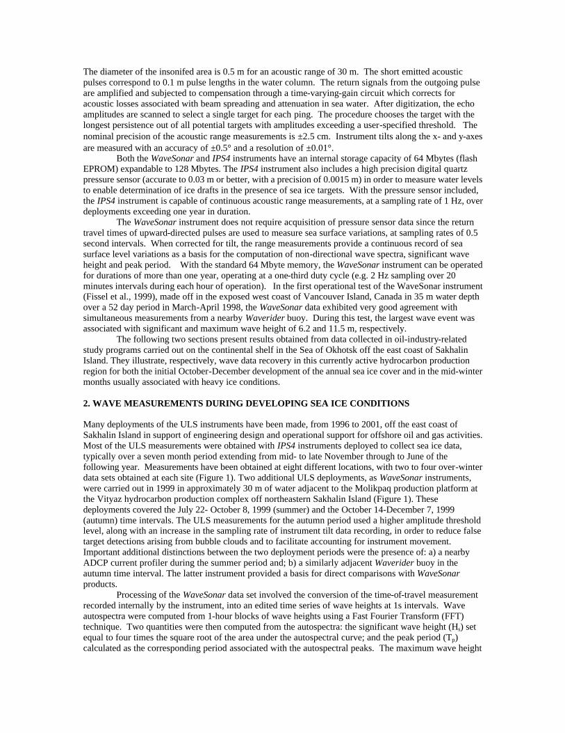
Significant wave height vs. peak period data and percentage wave height exceedences are plotted in Figures 3(a) and 3(b), respectively as extracted from the autumn data set associated with higher sea state conditions. The peak period results show frequent occurrences of larger wave events (Hs > 3 m) with periods in the 8 to 13 second range. Percentage exceedences for significant wave height (Hs) and maximum wave height (Hmax) show that 77% of the HS values were greater than 0.75 m, with 41% and 3% exceeding 1.5 m and 4 m, respectively. During this period, Hmax exceeded 1.5 m, 4 m and 7 m, 71%, 19% and 3.5% of the time, respectively.

Finally, comparisons of the obtained WaveSonar data were made with data acquired by a Waverider buoy deployed nearby from October 14 through December 2, 1999. The Waverider buoy transmitted wave data via a RF link to a receiver aboard the Okha tanker (located near the SALM site in Figure 1), as part of a real-time current/wave system installed near the Molikpaq for the 1999 operations season.

The “raw” Waverider wave height data were grouped into data blocks about 8 minutes in length. Comparisons with the WaveSonar 60-minute blocks of output data was facilitated by producing 3-point moving averages of the Waverider data to provide results equivalent to wave spectral characterization over approximately 20-odd minute sampling periods. The corresponding WaveSonar and Waverider data sets are plotted on the same graph for the period of overlap, Oct 14 – Dec 2 (Figure 4). The upper panel shows the wave heights (significant and max). The agreement in significant wave height is very good, within 5% or better. On two occasions (Nov 13-14 and Nov 26-27) the Waverider data was erratic due to buoy icing/depression. At these times, the WaveSonar data was unaffected by such effects due to the instrument being located on the seabed in a position well removed from direct contact with the ice and ocean surfaces. The peak period values obtained with the two alternative technologies show excellent agreement.

Overall, the autumn 1999 results effectively demonstrated the advantages of the WaveSonar for wave studies in areas in situations where sea-ice is developing and/or buoy icing is likely. More recently, portions of IPS4 data records associated with over-winter (November to June) periods have been extracted and analysed for ocean wave characteristics, during intervals associated with relatively ice free conditions. These efforts have resulted in a considerable body of wave climate information for the east coast of Sakhalin Island over the three year period (1996/97 to 1998/99). The analysed data were primarily acquired during the November to mid-December and late April to mid-June periods, when the surface conditions are characterized by open water with thin (< 0.3 m thick) developing ice and open water with remnants of highly dispersed and melting ice floes, respectively. More IPS4 data sets have also collected for the 2000/01 season (late November to early August), from which additional wave climate information can be derived.

0.0

2.0

4.0

6.0

8.0

10.0

12.0

10/14 10/19 10/24 10/29 11/03 11/08 11/13 11/18 11/23 11/28 12/03

Wave

Heigh

t (m)

Significant Wave Height

Max Wave Height

0.0

2.0

4.0

6.0

8.0

10.0

12.0

14.0

16.0

18.0

10/14 10/19 10/24 10/29 11/03 11/08 11/13 11/18 11/23 11/28 12/03

Time (1999 mm/dd)

Peak

Perio

d (s)

Figure 2. Significant wave height (Hs), maximum wave height (Hmax) and peak period (Tp) for the autumn 1999 data set.

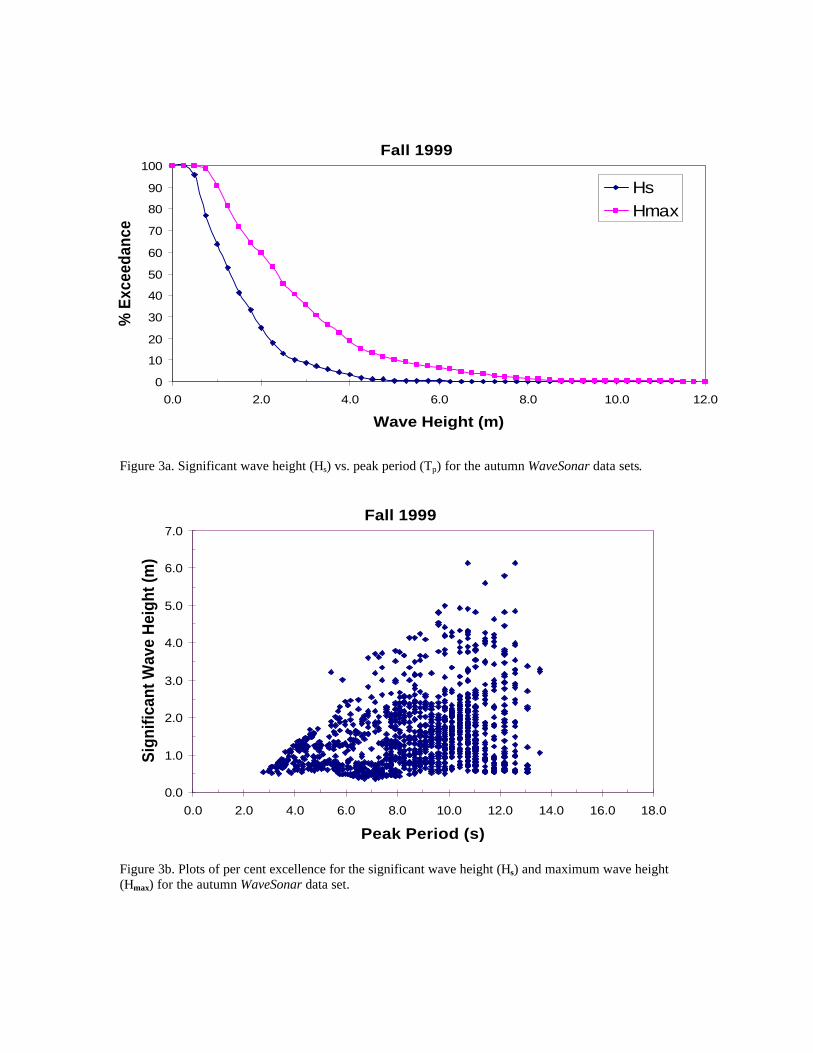
Figure 3a. Significant wave height (Hs) vs. peak period (Tp) for the autumn WaveSonar data sets.

Figure 3b. Plots of per cent excellence for the significant wave height (Hs) and maximum wave height (Hmax) for the autumn WaveSonar data set.

Fall 1999

0

10

20

30

40

50

60

70

80

90

100

0.0 2.0 4.0 6.0 8.0 10.0 12.0

Wave Height (m)

% E

xcee

danc

e

HsHmax

Fall 1999

0.0

1.0

2.0

3.0

4.0

5.0

6.0

7.0

0.0 2.0 4.0 6.0 8.0 10.0 12.0 14.0 16.0 18.0

Peak Period (s)

Sig

nific

ant W

ave

Hei

ght (

m)

0.0

2.0

4.0

6.0

8.0

10.0

12.0

10/14 10/19 10/24 10/29 11/03 11/08 11/13 11/18 11/23 11/28 12/03

Waverider Hmax

WaveSonar Hmax

0.0

2.0

4.0

6.0

8.0

10.0

12.0

14.0

16.0

18.0

10/14 10/19 10/24 10/29 11/03 11/08 11/13 11/18 11/23 11/28 12/03

Time (1999 mm/dd)

Waverider

WaveSonar

Figure 4. Significant wave height (Hs), maximum wave height (Hmax) and peak period (Tp) showing a comparison between the WaveSonar and Waverider instruments.

3. WAVE MEASUREMENTS IN WINTER WITHIN THE ICE PACK INTERIOR

The WaveSonar instrument is designed to return wave parameter data representative of relatively ice-free portions of ocean surfaces in the midst of occasional interference from local concentrations of ice floes or, even, thin layers of growing or melting slushy ice. The much weaker acoustic returns characteristically received by ULS instruments from ice (Melling, 1998) with drafts larger than about 40 cm yield far from optimal WaveSonar measurements under thicker pack ice. Consequently, detailed monitoring of wave activity in heavy pack ice from subsurface instruments has, to date, been accomplished with IPS4 Ice Profilers as part of seasonal ice study programs.

The effects of wave activity on the range or ice draft record obtained with such instruments is commonplace and to be expected during those periods in which seasonal or shorter term variations in pack position and/or extent bring the pack ice/open water boundary into the vicinity of the monitoring site. These changes allow wave penetration into the outer ice pack as a consequence of the usually low attenuation coefficients associated with the, typically, thinner and less concentrated ice characteristic of such areas. Nevertheless, results obtained during several years of intensive monitoring of the winter pack ice off Sakhalin Island (Birch et al., 2000) have shown significant frequencies of relatively long duration occurrences of large amplitude waves in interior portions of the ice pack, with thicknesses between 1.5 m and 2.5 m. Such wave propagation has been observed in pack ice hundreds of km from potential wave source regions.

Significant waves-in-ice events have been observed in the winters of 1997-1998, 1998-1999, and 2000-2001. Particularly intense events occurred in March 1998 and again in January 2001. Data on the first of these events will be presented here as gathered with an array (Figure 5) of 8 individual IPS4 instruments and adjacent current profiling and ice velocity-measuring instruments (which allowed the time series draft data collected by the IPS4 units to be converted in quasi-spatial series formats for offshore design purposes).

Figure 5. The Sakhalin Island monitoring area including the March 19 and March 21 5/10 ice concentration boundaries and e successive numbered positions of the centre of a traversing cyclone at 6-hour intervals during the event. Surface pressure contours (at 5 mb intervals from a 965 mb central contour are also included coincident with first wave arrivals

The wave activity in question was observed on March 20 and 21 at the 6 central sites in the regions that monitored ice conditions in spanning the 25m and 70m bathymetric contours. The closest of the affected monitoring sites was approximately 250 km from the 5/10 ice edge immediately prior to the local passage of the cyclone (see the positions of the cyclone center in Figure 5) which subsequently moved the same contour (indicated in the Figure) toward the Sakhalin coastline (and the monitoring sites) by, roughly, 80 km immediately prior to the observed wave event. These movements still left the outermost monitoring site (PA3) under 10/10 ice of 1.5 m mean thickness respective 155 km and 340 km from the nearest 5/10 and 1.6/10 ice boundaries.

Figure 6. Ice draft time series at site PA3 during a 10-minute period centred on Julian Day 79.9931 (2350, March 20, 1998).

Figure 7. Temporal spectra for periods encompassing peak activity at: PA3 (solid line, 0144- 0532, March 21); PA2 (connected dots, 0301-0712, March 21) and PA1 (dots, 0238-0712, March 21).

Nevertheless at, roughly, 20:00, March 20 a rapid and clearcut buildup of periodic range/draft signal was

noted, first at the outermost central sites and then, after considerable delays at the more shoreward monitoring locations. A typical segment of the time series record at times close to the event’s intensity peak is shown in Figure 6 as recorded at the outermost PA3 site. The wave amplitude in this case was sufficiently large, equivalent to, roughly, a 4 m significant wave height, that the draft variations in a highly deformed ice pack were barely discernable. Spectral analyses of peak amplitude signals at 3 successively more shore sites at, roughly, the same latitude (Figure 7) show the highly monochromatic nature of the wave spectrum which was centred on approximately 0.07 Hz (14 s wave periods). The lower frequency peaks in the Figure are artifacts of prior passages through a high pass filter to eliminate contributions from very low frequencies associated primarily with ice

undersurface topography. The results show the progressive decrease in wave amplitude as the waves advance shoreward through the ice pack and, as well, an accompanying shift to lower peak frequencies as a consequence of the well-known tendency of ice to act as a low-pass filter on incident wave fields.

The narrow width of the wave spectrum facilitated study of the observed event by allowing estimation of wave intensities at each site as a function of time in terms of the squared amplitude of the signal output after passage through a band pass filter with half power points at 0.066 Hz and 0.078 Hz. These intensities, plotted in Figure 8 along with superimposed time series of mean near-surface current vectors at each site, show both the considerable duration of the event at each (typically on the order of 24 hrs) but, as well, the its pronounced concentration at the 6 central sites and the steady falloff in intensity with distance from the eastern edge of the ice pack.

Figure 8. Filtered wave intensity-8dB plotted as a function of time in the period; 0000, March 19 – 1600, March 23 for each JIP site. Stick plot representations of total (residual + tidal) currents are also included.

Detailed comparisons of intensities and measurements of the time delays between the sharp rise in intensity

which marked the arrival of waves at each site allowed fairly refined estimates of wave attenuation/per unit length

(a) as a function of position in the ice pack and of the velocity of propagation associated with the advance of wave energy. Results were obtained from data collected at 3 different grouping of central sites. Attenuation results were, roughly, compatible with earlier estimates (Wadhams, 1986) from on-ice accelerometer data and directional analyses confirmed the expected westward propagation of waves generated by the cyclone’s position over open water in the eastern Sea of Okhotsk. The derived propagation speeds decreased with distance into the pack (and with increasing mean ice thickness) but were also anomalously low, corresponding to approximately 10% of the values associated with wave group speeds in open water as predicted by conventional theories of propagation in a floating ice plate (Wadhams, 1986, Squire, 1995). A detailed interpretation of these results (Marko, to be published) suggests that the measured propagation speed is associated with the spatial advance of a transition from high to low wave attenuation rates which is characteristic of wave propagation in pack ice subjected to divergent forcing immediately subsequent to an intense compression event. Aside from the interesting scientific issues raised by the observed propagation anomalies, these measurements demonstrated the capability of moored ULS wave monitoring under a continuum of conditions in ice–infested waters. 4. CONCLUSIONS AND RELATED DEVELOPMENTS

The capability of ULS instruments to provide reliable ocean wave measurements has been demonstrated by

the good agreement achieved between WaveSonar and Datawell Waverider measurements in the autumn of 1999 off Sakhalin Island. During this same measurement program, the greater data recovery rate of the sonar measurements was also evident as a consequence of the WaveSonar’s in capability for operating under conditions in which structural icing and the presence of thin sea ice interfered with Waverider operation.

The IPS4 version of the ULS instrumentation was also used effectively to provide a unique data associated with ocean waves propagating within seasonal pack ice off Sakhalin Island. These results were of considerable relevance to models of marginal pack ice and demonstrated the capabilities of ULS wave monitoring technique for wave studies in pack ice interiors.

Recently, a hybrid version of the IPS4 and WaveSonar instrument has been developed for use over a full one year period in the Canadian sector of the Beaufort Sea. The first version of this instrument, operating at the usual 420 Khz acoustic frequency was deployed in September 2001 and will be recovered in September 2002. The instrument has been operated in various pre-set data collection phases. In winter, the hybrid instrument is operated as an IPS4 unit, sampling at 2 second intervals, with a relatively high gain to allow detection of the weak sea ice back scatter returns. In the summer and early autumn periods, when ocean waves are present, the instrument also provides a burst sampling mode to measure waves for 2048 seconds every 3 hours, sampling at 2 Hz using the lower sonar gain, while at the same time continuing to provide sea ice detection at higher gains and a lower sampling rate (0.5 Hz). A more advanced version of the hybrid IPS4/WaveSonar is now under development. This new version will feature a smaller acoustic beamwidth (1.4 degrees) operating at a higher acoustic frequency (900 Khz) than the present ULS instrumentation (1.8 degrees beamwidth at 420 Khz) so as to provide improved horizontal resolution and an increased potential for carrying out wave studies at sampling rates greater than 2 Hz. 5. REFERENCES Birch, J.R, D. Fissel, H. Melling, K. Vaudrey, K. Schaudt, J. Heideman and W. Lamb. 2000: Ice Profiling Sonar: Upward looking sonar provides over-winter records of ice thickness and ice keel depths off Sakhalin Island, Russia. Sea Technology, 41(8), 48-53. Fissel, D., R. Birch, Borg, K., and Melling, H. 1999: Wave Measurements Using Upward-Looking Sonar for Continental Shelf Applications. Proc. Offshore Tech. Conference (Paper # 10794), Houston, TX. Marko, J.R. 2002: Observations and analyses of an intense waves-in-ice event in the interior of the Sea of Okhotsk ice pack. J. Geophys. Res., 107, (accepted for publication). Melling, H., 1998: Sound scattering from sea ice: aspects relevant to ice-draft profiling by sonar. J. Atm. Oceanic Tech., 15, 1023-1034. Melling, H., P.H. Johnston and D.A. Reidel, 1995: Measurement of the draft and topography of sea ice by moored sub-sea sonar J. Atmos. Oc. Tech., 12, 589-609. Macovsky, M.L. and G. Mechlin, 1963. A proposed technique for obtaining wave spectra by an array of inverted fathometers. In Ocean Wave Spectra, Prentice-Hall, Englewood Cliffs, N.J., 235-241. Squire, V.A., 1995, Geophysical and oceanographic information in the marginal ice zone from ocean wave measurements, J. Geophys. Res., 100, pp.997-998.

Wadhams, P. 1986: The seasonal ice zone. in The Geophysics of Sea Ice (N. Untersteiner, ed.), Plenum Press, New York and London, 825-991.