Wavelets and Edge Detection CS698 Final Project

Submitted To: Professor Richard Mann

Submitted By: Steve Hanov Course: CS698

Date: April 10, 2006

INTRODUCTION Wavelets have had a relatively short and troubled

history. They seem to be forever confined to footnotes in textbooks on Fourier theory. It seems

that there is little that can be done with wavelets

that cannot be done with traditional Fourier

analysis.

Stephane Mallat was not the father of wavelet

theory, but he is certainly an evangelist. His textbook on the subject, A Wavelet Tour of Signal

Processing [1], contains proofs about the theory of

wavelets, and a summation about what is known

about them with applications to signal processing. One of his many papers, Characterization of

Signals from Multiscale Edges [2], is frequently

cited as a link between wavelets and edge detection. Mallat’s method not only finds edges,

but classifies them into different types as well.

Mallat goes on to describe a method of recovering complete images using only the edges, but we will

not implement it in this project. In this project, we

study this paper, and implement the method of

Mallat to multiscale edge detection and analysis.

We will first present a short background on

wavelet theory. Then we will describe the different types of edges that exist in images, and how they

can be characterized using a Lipschitz constant.

Next, we describe the algorithm for the wavelet transform, from the Mallat paper. Finally, we

show the results of applying the algorithm to a test

image, and a real image.

WAVELET ANALYSIS

THEORY

It is best to describe wavelets by showing how they differ from Fourier methods. A signal in the

time domain is described by a function f(t), where

t is usually a moment in time. When we apply the Fourier transform to the signal, we obtain a

function F(ω) that takes as input a frequency, and outputs a complex number describing the strength

of that frequency in the original signal. The real

part is the strength of the cosine of that frequency, and the imaginary part is the strength of the sine.

One way to obtain the Fourier transform of a signal is to repeatedly correlate the sine and cosine

wave with the signal. When the results high

valued, the coefficients of the Fourier transform will be high. Where the signal or the wave is close

to zero, the coefficients will be low.

Fourier analysis has a big problem, however. The sine and cosine functions are defined from -∞ to ∞. The effects of each frequency are analyzed as if

they were spread over the entire signal. For most signals, this is not the case. Consider music, which

is continuously varying in pitch. Fourier analysis

done on the entire song tells you which frequencies exist, but not where they are.

The short time Fourier transform (STFT) is often

used when the frequencies of the signal vary greatly with time. [3] In the JPEG image encoding

standard, for example, the image is first broken up

into small windows with similar characteristics. The Fourier transform is not applied to the entire

image, but only to these small blocks. The

disadvantage of this technique can be seen at high compression ratios, when the outlines of the

blocks are clearly visible artifacts.

A second disadvantage is in resolution of analysis. When larger windows are used, lower frequencies

can be detected, but their position in time is less

certain. With a smaller window, the position can be determined with greater accuracy, but lower

frequencies will not be detected.

The wavelet transform helps solve this problem. Once applied to a function f(t), it provides a set of

functions Wsf(t). Each function describes the

strength of a wavelet scaled by factor s at time t. The wavelet extends for only a short period, so its

effects are limited to the area immediately

surrounding t. The wavelet transform will give information about the strengths of the frequencies

of a signal at time t.

In the first pages of his treatise [1], Mallat defines a wavelet as a function of zero average,

∫∞∞−

= 0)( dttψ

which is dilated with scale parameter s, and translated by u:

−=

s

ut

stsu ψψ

1)(,

Unlike the sine and cosine functions, wavelets

move toward quickly zero as their limits approach

to +/-∞.

In [2], Mallat notes that the derivative of a

smoothing function is a wavelet with good

properties. Such a wavelet is shown in Figure 1.

0 100 200 300 400 500 6000

0.1

0.2

0.3

0.4

0.5

0.6

0.7

0.8

0.9

1

0 100 200 300 400 500 600-0.4

-0.3

-0.2

-0.1

0

0.1

0.2

0.3

0.4

Figure 1: A smoothing function, and its corresponding

wavelet.

By correlating the signal with this function at all

possible translations and scales, we obtain the continuous wavelet transform.

The transformation also increases the dimension of

the function by one. Since we have both a scaling and position parameter, a 1-D signal will have a 2-

D wavelet transform. As an illustration, in Figure

2 we show the wavelet transform of a single scan line of an image, calculated using the algorithm in

[2] (See Appendix A). The frequencies decrease

from top to bottom, and pixel position increases

from left to right. The edges in the signal result in funnel-shaped patterns in the wavelet transform.

Figure 2: The 512th scanline of the famous Lena image,

and its wavelet transform. Pixel position increases from

left to right, and frequency increases from bottom to top.

Only nine scales were used, but they are stretched to

simulate a continuous transform, which is more

illustrative.

Like the Fourier transform, the wavelet transform

is invertible. However, it is easier to throw away information based on position. In the Fourier

domain, if you were to try to eliminate noise by

simply throwing away all of the information in a certain frequency band, you would get back a

smoothed signal, with rounded corners, because all

frequencies contribute to larger structures in all parts of the signal. With the wavelet transform,

however, it is possible to selectively throw out

high frequencies in areas where they do not

contribute to larger structures. Indeed, this is the idea behind wavelet compression.

Here is the scan line from the Lena image, with the highest frequency wavelet coefficients

removed:

0 100 200 300 400 500 6000

50

100

150

200

250reconstructed

The signal keeps the same structure as the original,

but is smoother. Here is the same signal with the three highest dyadic

1 frequency bands removed:

0 100 200 300 400 500 6000

50

100

150

200

250reconstructed

The signal is smoother, but the edges are rounder.

So far, this frequency removal is equivalent to smoothing the signal with a Gaussian. The true

power of the wavelet transform is revealed,

however, when we selectively remove wavelet coefficients from the first three dyadic frequency

bands only in positions where they are weak (in

this case, less than +/-20):

0 100 200 300 400 500 6000

50

100

150

200

250

reconstructed

Here, the signal retains much of its original

character. Most edges remain sharp. This simple

algorithm for noise removal could be improved

further if it did not change the weak coefficients in areas where they contribute to the larger structure.

To do this, one would need to consider the

coefficients across all scales, and determine the positions of the edges of the signal. In his paper,

Mallat presents a way to do just that.

WAVELET TRANSFORM TYPES There are numerous types of wavelet transforms. The first is the continuous wavelet transform

(CWT). Dispite its name, the wavelet transform

can be calculated on discrete data. All possible scaling factors are used, starting at 1 and

increasing to the number of samples in the signal.

However, the CWT is computationally expensive, and for most applications, a dyadic method is used

instead.

1 Dyadic: based on successive powers of two

In the dyadic wavelet transform, we use only

scales that are powers of two. With the careful choice of an appropriate wavelet,

this covers the entire frequency domain. At the

scale s=1, the image is smoothed by convolving it

with a smoothing function. At scale s=2, the smoothing function is stretched, and the image is

convolved with it again. The process is repeated

for s=4, s=8, etc., until the smoothing function is as large as the image. At each level, the wavelet

transform contains information for every position t

in the image. This method is used by Mallat.

Most applications today, however, use an even

more optimal method. Since the image is

smoothed at each step by a filter, the image only contains half of the frequency information, and

needs half as many samples. So the number of

samples in the image is reduced at each stage as well. As a result, the wavelet transform is reduced

to the same size as the original signal. Mallat

avoids this optimization because he needs the redundant information to recover the image using

only its modulus maxima (edges).

CHARACTERIZATION OF EDGES When the wavelet transform is used with a

smoothing function, it is equivalent to Canny edge detection [4]. The derivative of a Gaussian is

convolved with the image, so that local maxima

and minima of the image correspond to edges.

Note Figure 2, in which large drops are characterized by black funnels, and leaps result in

white funnels. It is clear that by examining the

wavelet transform, we can extract a lot of information about the edges. For example, we can

see whether it is a gradual change or a leap, or

whether it is a giant cliff, or a momentary spike, by looking only at the wavelet representation.

Edges are characterized mathematically by their

Lipschitz regularity. We say that a function is

uniformly Lipschitz α, over the interval (a,b), if, and only if, for every x, x0 in the interval, there is

some constant K such that:

α

yxKxfxf −≤− )()( 0

The area over the interval will never have a slope

that is steeper than the constant K. [5]

Mallat shows that the Lipschitz continuity is

related to the wavelet transform, and that if the

wavelet transform is Lipschitz α, the function is

also Lipschitz α:

α)2()(

2

jKxfW j ≤

The conclusions are summarized in the following

table.

αααα constraint Meaning Impact on

Wavelet

transform

0 < α <= 1 f(x) is

differentiable at

x0. The change is gradual.

Amplitude

decreases

with scale.

α = 0 F(x) is not

differentiable at

x0. A sharp change or

discontinuity

exists.

Amplitude

remains

the same across

scales.

-1 <= α < 0 F(x) is an impulse

at x0.

Amplitude

decreases

with scale.

In Figure 3, an artificial 1-D signal is shown to

illustrate the effects of a variety of edge types on

the dyadic wavelet transform.

Figure 3

The algorithm can be extended to 2 dimensions.

We say that a 2-D image is Lipschitz α in the box (x0, y0) – (x1, y2) if and only if there is a constant

K, such that for any two points in the box, [2]

2/2

0

2

000 )(),(),(α

yyxxKyxfyxf −+−≤−

EDGE DETECTION ALGORITHM The algorithm for performing the edge detection is as follows. In the following examples, this source

image will be used.

When the wavelet transform of the image is

performed, it results in two stacks of images. Since

the image is 256x256 pixels, eight scaling levels

are used, and each stack contains eight images. One image stack contains the separable horizontal

filtering, and the other contains the vertical

filtering. In the pictures that follow, the scaling

factor s=4 is shown. However, the algorithm is performed at all dyadic scaling levels.

At each step, the image is convolved with a wavelet to obtain the coefficients at that level. It is

then smoothed with a Gaussian of increasing scale.

Both the wavelet and Gaussian filtering is done using separate 1-D filters vertically and

horizontally.

Figure 4: ),(1 yxfWs

and ),(2 yxfWs

The modulus maxima image combines the two

filtered images, and it is calculated using the formula:

2221 ),(),(),( yxfWyxfWyxfM sss +=

The angular image is calculated using

),(

),(arctan

1

2

yxfW

yxfW

s

s

The result is shown below. The horizontal and

vertical images form a gradiant image. The modulus maxima image is the scalar value of the

vector at each point, and the angular image is the

angle. In the angular image, low values represent 0

degrees from the horizontal, and higher values represent 90 degrees.

Modulus Maxima Angular Image

Finally, the lines of the maxima are found, using the information from both the modulus and

angular image. Curiously, Mallat does not use a

2nd

derivative to find them. Instead, he proposes a simple algorithm. A five point discrete derivative

function was tried for this, but it did not perform

better than Mallat’s simple algorithm. A pixel is a

modulus maximum if it is larger than its two neighbours long the angle of the gradient vector.

A pixel has only eight neighbours, however. In my

implementation of the algorithm, the angles from 0

to 2π are divided into 45° sections as illustrated in

the figure below, so that two of the eight neighbouring pixels can be chosen to be compared

to the centre pixel.

45°

Figure 5: Angles are divided into sections to choose the

maxima among neighbouring pixels.

To help detect only salient features, the maxima with a value above a certain threshold are taken

and plotted.

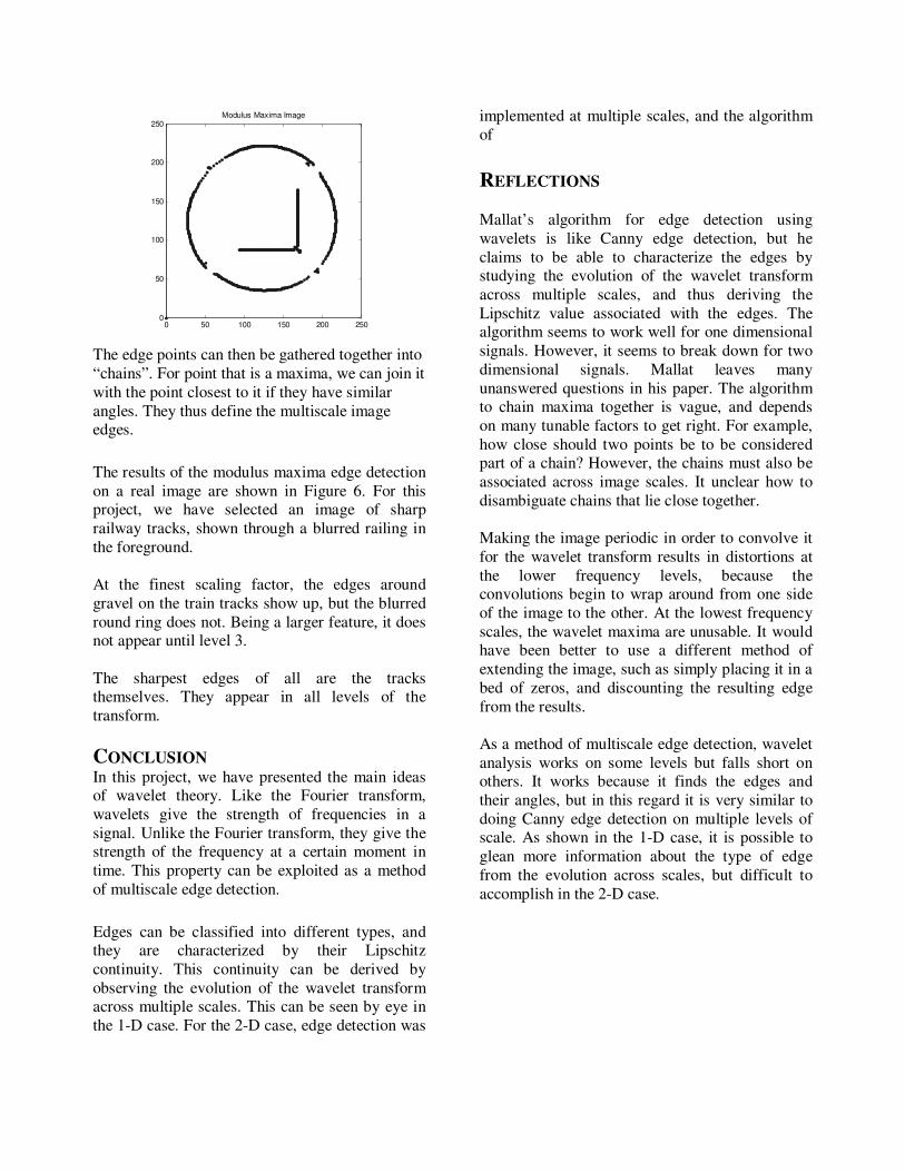
0 50 100 150 200 2500

50

100

150

200

250Modulus Maxima Image

The edge points can then be gathered together into

“chains”. For point that is a maxima, we can join it

with the point closest to it if they have similar

angles. They thus define the multiscale image edges.

The results of the modulus maxima edge detection

on a real image are shown in Figure 6. For this project, we have selected an image of sharp

railway tracks, shown through a blurred railing in

the foreground.

At the finest scaling factor, the edges around

gravel on the train tracks show up, but the blurred

round ring does not. Being a larger feature, it does not appear until level 3.

The sharpest edges of all are the tracks themselves. They appear in all levels of the

transform.

CONCLUSION In this project, we have presented the main ideas of wavelet theory. Like the Fourier transform,

wavelets give the strength of frequencies in a

signal. Unlike the Fourier transform, they give the strength of the frequency at a certain moment in

time. This property can be exploited as a method

of multiscale edge detection.

Edges can be classified into different types, and they are characterized by their Lipschitz

continuity. This continuity can be derived by

observing the evolution of the wavelet transform across multiple scales. This can be seen by eye in

the 1-D case. For the 2-D case, edge detection was

implemented at multiple scales, and the algorithm

of

REFLECTIONS Mallat’s algorithm for edge detection using

wavelets is like Canny edge detection, but he

claims to be able to characterize the edges by studying the evolution of the wavelet transform

across multiple scales, and thus deriving the

Lipschitz value associated with the edges. The algorithm seems to work well for one dimensional

signals. However, it seems to break down for two

dimensional signals. Mallat leaves many

unanswered questions in his paper. The algorithm to chain maxima together is vague, and depends

on many tunable factors to get right. For example,

how close should two points be to be considered part of a chain? However, the chains must also be

associated across image scales. It unclear how to

disambiguate chains that lie close together.

Making the image periodic in order to convolve it

for the wavelet transform results in distortions at

the lower frequency levels, because the convolutions begin to wrap around from one side

of the image to the other. At the lowest frequency

scales, the wavelet maxima are unusable. It would have been better to use a different method of

extending the image, such as simply placing it in a

bed of zeros, and discounting the resulting edge

from the results.

As a method of multiscale edge detection, wavelet

analysis works on some levels but falls short on others. It works because it finds the edges and

their angles, but in this regard it is very similar to

doing Canny edge detection on multiple levels of scale. As shown in the 1-D case, it is possible to

glean more information about the type of edge

from the evolution across scales, but difficult to

accomplish in the 2-D case.

WAVELET TRANSFORM AND EDGE DETECTION OF AN IMAGE

A0 100 200 300 400 500 600

0

100

200

300

400

500

600

B0 100 200 300 400 500 600

0

100

200

300

400

500

600

C0 100 200 300 400 500 600

0

100

200

300

400

500

600

D0 100 200 300 400 500 600

0

100

200

300

400

500

600

E0 100 200 300 400 500 600

0

50

100

150

200

250

300

350

400

450

F0 100 200 300 400 500 600

0

50

100

150

200

250

300

350

400

450

G0 100 200 300 400 500 600

0

50

100

150

200

250

300

350

400

450

500

H Figure 6: The wavelet transform and exact modulus maximus detection applied to a test image. H is the original image, and A-

G are the modulus maxima at increasing levels of scaling factors. The last image, G, is distorted due to wrapping of the image

for convolution.

Appendix A – Matlab Source Code

The dwt function calculates the dyadic wavelet transform of a 1-D function, using the algorithm described in

[2]. The wavelets used are the ones described in the same paper, and pictured in Figure 1. In all of this code, the Matlab mod function is used to make the input signal appear to be periodic, for the purposes of

convolution. For example, if you wanted to extract the12th element of an eight pixel scan line, mod( 12-1,

8)+1 would calculate the correct pixel index to be 4. function [W] = dwt( F ) SizeF = size(F); N = SizeF(1); % N should be a power of two. J = log(N)/log(2); W = zeros(N, J+1); % Prepare normalization coefficients LambdaTable = [ 1.50 1.12 1.03 1.01 ]; figure; plot(F); title('Original Signal'); j = 0; while j < J p = 2 ^ j - 1; % Which normalization coefficient to use? Lambda = 1; if j < 4 Lambda = LambdaTable(j+1); end % convolve the function with G, as if G has 2^j-1 zeros in between the % coefficients. for i = 1:N W(i,j+1) = (-2 * F(i) + 2 * F ( mod( i + p, N ) + 1 )) / Lambda; end %figure; %plot(W(:,j+1)); % To get the next version of F, convolve it with H,, if H has w^j - 1 % zeros between the coefficients. S = zeros(N,1); for i = 1:N S(i) = 0.125 * F( mod( i - p - 2, N) + 1 ) + ... 0.375 * F(i) + ... 0.375 * F( mod( i + p, N ) + 1 ) + ... 0.125 * F( mod( i + p * 2 + 1, N ) + 1 ); end F = S; j = j + 1; end W(:,J+1) = S;

The 1-D inverse wavelet transform is also implemented: function [S] = idwt( W ) [N, J] = size(W); S = W(:,J); J = J - 1; j = J; % Prepare normalization coefficients LambdaTable = [ 1.50 1.12 1.03 1.01 ]'; while j > 0 p = 2 ^ (j-1) - 1; % Number of zeros between H, G, K coefficients

% Which normalization coefficient to use? Lambda = 1; if j < 4 Lambda = LambdaTable(j); end % Calculate the K part K = zeros(N, 1); for i = 1:N K(i) = 0.0078125 * W( mod( i - 3*p - 4, N) + 1, j ) + ... 0.054685 * W( mod( i - 2*p - 3, N) + 1, j ) + ... 0.171875 * W( mod( i - p - 2, N) + 1, j ) + ... -0.171875 * W( i, j ) + ... -0.054685 * W( mod( i + p , N) + 1, j ) + ... -0.0078125 * W( mod( i + p * 2 + 1 , N) + 1, j ); end % Calculate the ~H part. H = zeros(N, 1); for i = 1:N H(i) = 0.125 * S(mod( i - 2*p - 3, N ) + 1 ) + ... 0.375 * S(mod( i - p - 2, N ) + 1 ) + ... 0.375 * S(i) + ... 0.125 * S(mod( i +p, N ) + 1 ); end S = K * Lambda + H; j = j - 1; end

The dwt2 function calculates the dyadic wavelet transform of a two dimensional image. It returns a three

dimensional matrix W, which is a stack images representing the wavelet transform at dyadic scales. function [Wx, Wy] = dwt2( F ) SizeF = size(F); N = SizeF(1); J = log(N)/log(2); Wx = zeros(N, N, J+1); Wy = zeros(N, N, J+1); LambdaTable = [ 1.50 1.12 1.03 1.01 ]; figure; imshow( F ); title('Original Signal'); S = zeros(N,N); figure; j = 0; while j < J p = 2 ^ j - 1; % Which normalization coefficient to use? Lambda = 1; if j < 4 Lambda = LambdaTable(j+1); end for y = 1:N for x = 1:N Wx(y,x,j+1) = (-2 * F(y,x) + ... 2 * F(y,mod(x+p,N)+1) ) / Lambda; Wy(y,x,j+1) = (-2 * F(y,x) + ... 2 * F(mod(y+p,N)+1,x) ) / Lambda; S(y,x) = 0.125 * F( y, mod( x - p - 2, N) + 1 ) + ... 0.375 * F(y, x) + ...

0.375 * F(y, mod( x + p, N ) + 1 ) + ... 0.125 * F(y, mod( x + p * 2 + 1, N ) + 1 ) + ... 0.125 * F( mod( y - p - 2, N) + 1, x ) + ... 0.375 * F(y, x) + ... 0.375 * F(mod( y + p, N ) + 1,x ) + ... 0.125 * F( mod( y + p * 2 + 1, N ) + 1,x ); end end subplot(J,2,j*2+1); imshow(Wx(:,:,j+1), [min(min(Wx(:,:,j+1))) max(max(Wx(:,:,j+1)))]); subplot(J,2,j*2+2); imshow(Wy(:,:,j+1), [min(min(Wy(:,:,j+1))) max(max(Wy(:,:,j+1)))]); F = S; j = j + 1; end %W(:,:,J+1) = S; figure; imshow(S, 256); Here, we use the inverse dwt on the 1-d scanline of the lena image, to remove noise below a certain threshold,

but retain the sharp features where strong coefficients exist.

I = double(imread('lena.png')); Size = 512; M = I(512,:)'; W = dwt(M); for j = 1:3 for i = 1:512 if abs(W(i,j)) < 20 W(i,j) = 0; end end end F = idwt(W); figure; plot(F); title('reconstructed'); figure; imshow( W', [ min(min(W)) max(max(W)) ] );

REFERENCES 1 S. Mallat, A Wavelet Tour of Signal Processing, London: Academic Press, 1999

2 S. Mallat, “Characterization of Signals from Multiscale Edges,” IEEE. Trans. Patt. Anal. Machine Intell., vol. PAMI-

14, pp. 710-732, 1992.

3 R. Polikar – The Wavelet Tutorial. http://users.rowan.edu/~polikar/WAVELETS/WTtutorial.html 4 J. Canny, “A computational approach to edge detection,” IEEE Trans. Patt. Anal. Machine Intell., vol. PAMI-8, pp.

679-698, 1986.

5 Wikipedia. “Lipschitz Continuity,” http://en.wikipedia.org/wiki/Lipschitz_continuity