Where is the Land of Opportunity?The Geography of Intergenerational Mobility in the United States∗

Raj Chetty, Harvard University and NBERNathaniel Hendren, Harvard University and NBER

Patrick Kline, UC-Berkeley and NBEREmmanuel Saez, UC-Berkeley and NBER

June 2014

Abstract

We use administrative records on the incomes of more than 40 million children and their parentsto describe three features of intergenerational mobility in the United States. First, we charac-terize the joint distribution of parent and child income at the national level. The conditionalexpectation of child income given parent income is linear in percentile ranks. On average, a10 percentile increase in parent income is associated with a 3.4 percentile increase in a child’sincome. Second, intergenerational mobility varies substantially across areas within the U.S. Forexample, the probability that a child reaches the top quintile of the national income distribu-tion starting from a family in the bottom quintile is 4.4% in Charlotte but 12.9% in San Jose.Third, we explore the factors correlated with upward mobility. High mobility areas have (1)less residential segregation, (2) less income inequality, (3) better primary schools, (4) greatersocial capital, and (5) greater family stability. While our descriptive analysis does not iden-tify the causal mechanisms that determine upward mobility, the publicly available statistics onintergenerational mobility developed here can facilitate research on such mechanisms.

∗The opinions expressed in this paper are those of the authors alone and do not necessarily reflect the views of theInternal Revenue Service or the U.S. Treasury Department. This work is a component of a larger project examiningthe effects of tax expenditures on the budget deficit and economic activity. All results based on tax data in thispaper are constructed using statistics originally reported in the SOI Working Paper “The Economic Impacts of TaxExpenditures: Evidence from Spatial Variation across the U.S.,” approved under IRS contract TIRNO-12-P-00374and presented at the National Tax Association meeting on November 22, 2013. We thank David Autor, Gary Becker,David Card, David Dorn, John Friedman, James Heckman, Nathaniel Hilger, Richard Hornbeck, Lawrence Katz,Sara Lalumia, Adam Looney, Pablo Mitnik, Jonathan Parker, Laszlo Sandor, Gary Solon, Danny Yagan, numerousseminar participants, and four anonymous referees for helpful comments. Sarah Abraham, Alex Bell, Shelby Lin, AlexOlssen, Evan Storms, Michael Stepner, and Wentao Xiong provided outstanding research assistance. This researchwas funded by the National Science Foundation, the Lab for Economic Applications and Policy at Harvard, theCenter for Equitable Growth at UC-Berkeley, and Laura and John Arnold Foundation. Publicly available portionsof the data and code, including intergenerational mobility statistics by commuting zone and county, are available atwww.equality-of-opportunity.org.

I Introduction

The United States is often hailed as the “land of opportunity,” a society in which a child’s chances

of success depend little on his family background. Is this reputation warranted? We show that this

question does not have a clear answer because there is substantial variation in intergenerational

mobility across areas within the U.S. The U.S. is better described as a collection of societies, some

of which are “lands of opportunity” with high rates of mobility across generations, and others in

which few children escape poverty.

We characterize intergenerational mobility using information from de-identified federal income

tax records, which provide data on the incomes of more than 40 million children and their parents

between 1996 and 2012. We organize our analysis into three parts.

In the first part, we present new statistics on intergenerational mobility in the U.S. as a whole.

In our baseline analysis, we focus on U.S. citizens in the 1980-1982 birth cohorts – the oldest

children in our data for whom we can reliably identify parents based on information on dependent

claiming. We measure these children’s income as mean total family income in 2011 and 2012, when

they are approximately 30 years old. We measure their parents’ income as mean family income

between 1996 and 2000, when the children are between the ages of 15 and 20.1

Following the prior literature (e.g., Solon 1999), we begin by estimating the intergenerational

elasticity of income (IGE) by regressing log child income on log parent income. Unfortunately, we

find that this canonical log-log specification yields very unstable estimates of mobility because the

relationship between log child income and log parent income is non-linear and the estimates are

sensitive to the treatment of children with zero or very small incomes. When restricting the sample

between the 10th and 90th percentile of the parent income distribution and excluding children with

zero income, we obtain an IGE estimate of 0.45. However, alternative specifications yield IGEs

ranging from 0.26 to 0.70, spanning most of the estimates in the prior literature.2

To obtain a more stable summary of intergenerational mobility, we use a rank-rank specification

similar to that used by Dahl and DeLeire (2008). We rank children based on their incomes relative

to other children in the same birth cohort. We rank parents of these children based on their incomes

relative to other parents with children in these birth cohorts. We characterize mobility based on the

1We show that our baseline measures do not suffer from significant lifecycle or attenuation bias (Solon 1992,Zimmerman 1992, Mazumder 2005) by establishing that estimates of mobility stabilize by the time children reachage 30 and are not very sensitive to the number of years used to measure parent income.

2In an important recent study, Mitnik et al. (2014) propose a new dollar-weighted measure of the IGE and showthat it yields more stable estimates. We discuss the differences between the new measure of mobility proposed byMitnik et al. and the canonical definition of the IGE in Section IV.A.

1

slope of this rank-rank relationship, which identifies the correlation between children’s and parents

positions in the income distribution.3

We find that the relationship between mean child ranks and parent ranks is almost perfectly

linear and highly robust to alternative specifications. A 10 percentile point increase in parent rank

is associated with a 3.41 percentile increase in a child’s income rank on average. Children’s college

attendance and teenage birth rates are also linearly related to parent income ranks. A 10 percentile

point increase in parent income is associated with a 6.7 percentage point (pp) increase in college

attendance rates and a 3 pp reduction in teenage birth rates for women.

In the second part of the paper, we characterize variation in intergenerational mobility across

commuting zones (CZs). Commuting zones are geographical aggregations of counties that are

similar to metro areas but cover the entire U.S., including rural areas (Tolbert and Sizer 1996). We

assign children to commuting zones based on where they lived at age 16 – i.e., where they grew

up – irrespective of whether they left that CZ afterward. When analyzing CZs, we continue to

rank both children and parents based on their positions in the national income distribution, which

allows us to measure children’s absolute outcomes as we discuss below.

The relationship between mean child ranks and parent ranks is almost perfectly linear within

commuting zones, allowing us to summarize the conditional expectation of a child’s rank given

his parents’ rank with just two parameters: a slope and intercept. The slope measures relative

mobility : the difference in outcomes between children from top vs. bottom income families within

a CZ. The intercept measures the expected rank for children from families at the bottom of the

income distribution. Combining the intercept and slope for a CZ, we can calculate the expected

rank of children from families at any given percentile p of the national parent income distribution.

We term this measure absolute mobility at percentile p. Measuring absolute mobility is valuable

because increases in relative mobility have ambiguous normative implications, as they may be

driven by worse outcomes for the rich rather than better outcomes for the poor.

We find substantial variation in both relative and absolute mobility across CZs. Relative mo-

bility is lowest for children who grew up in the Southeast and highest in the Mountain West and

the rural Midwest. Some CZs in the U.S. have relative mobility comparable to the highest mobility

countries in the world, such as Canada and Denmark, while others have lower levels of mobility

than any developed country for which data are available.

3The rank-rank slope and IGE both measure the degree to which differences in children’s incomes are determinedby their parents’ incomes. We discuss the conceptual differences between the two measures in Section II.

2

We find similar geographical variation in absolute mobility. We focus much of our analysis on

absolute mobility at p = 25, which we term “absolute upward mobility.” This statistic measures

the mean income rank of children with parents in the bottom half of the income distribution given

linearity of the rank-rank relationship. Absolute upward mobility ranges from 35.8 in Charlotte

to 46.2 in Salt Lake City among the 50 largest CZs. A 1 standard deviation (SD) increase in

CZ-level upward mobility is associated with a 0.2 SD improvement in a child’s expected rank given

parents at p = 25, 60% as large as the effect of a 1 SD increase in his own parents’ income. Other

measures of upward mobility exhibit similar spatial variation. For instance, the probability that a

child reaches the top fifth of the income distribution conditional on having parents in the bottom

fifth is 4.4% in Charlotte, compared with 10.8% in Salt Lake City and 12.9% in San Jose. The

CZ-level mobility statistics are robust to adjusting for differences in the local cost-of-living, shocks

to local growth, and using alternative measures of income.

Absolute upward mobility is highly correlated with relative mobility: areas with high levels of

relative mobility (low rank-rank slopes) tend to have better outcomes for children from low-income

families. On average, children from families below percentile p = 85 have better outcomes when

relative mobility is greater; those above p = 85 have worse outcomes. Location matters more for

children growing up in low income families: the expected rank of children from low-income families

varies more across CZs than the expected rank of children from high income families.

The spatial patterns of the gradients of college attendance and teenage birth rates with respect

to parent income across CZs are very similar to the variation in intergenerational income mobility.

This suggests that the spatial differences in mobility are driven by factors that affect children while

they are growing up rather than after they enter labor market.

In the final part of the paper, we explore such factors by correlating the spatial variation

in mobility with observable characteristics. To begin, we show that upward income mobility is

significantly lower in areas with larger African-American populations. However, white individuals

in areas with large African-American populations also have lower rates of upward mobility, implying

that racial shares matter at the community level.

We then identify five factors that are strongly correlated with the variation in upward mobility

across areas. The first is segregation: areas that are more residentially segregated by race and

income have lower levels of mobility. Second, areas with more inequality as measured by Gini coef-

ficients have less mobility, consistent with the “Great Gatsby curve” documented across countries

(Krueger 2012, Corak 2013). Top 1% income shares are not highly correlated with intergenera-

3

tional mobility both across CZs within the U.S. and across countries, suggesting that the factors

that erode the middle class may hamper intergenerational mobility more than the factors that

lead to income growth in the upper tail. Third, proxies for the quality of the K-12 school system

are positively correlated with mobility. Fourth, social capital indices (Putnam 1995) – which are

proxies for the strength of social networks and community involvement in an area – are also posi-

tively correlated with mobility. Finally, mobility is significantly lower in areas with weaker family

structures, as measured e.g. by the fraction of single parents. As with race, parents’ marital status

does not matter purely through its effects at the individual level. Children of married parents also

have higher rates of upward mobility in communities with fewer single parents. Interestingly, we

find no correlation between racial shares and upward mobility once we control for the fraction of

single parents in an area.

We find modest correlations between upward mobility and local tax policies and no systematic

correlation between mobility and local labor market conditions, rates of migration, or access to

higher education. In a multivariable regression, the five key factors described above generally

remain statistically significant predictors of both relative and absolute upward mobility, even in

specifications with state fixed effects. However, we emphasize that these factors should not be

interpreted as causal determinants of mobility because all of these variables are endogenously

determined and our analysis does not control for numerous other unobserved differences across

areas.

Our results build on an extensive literature on intergenerational mobility, reviewed by Solon

(1999) and Black and Devereux (2011). Our estimates of the level of mobility in the U.S. as

a whole are broadly consistent with prior results, with the exception of Mazumder’s (2005) and

Clark’s (2014) IGE estimates, which imply much lower levels of intergenerational mobility. We

discuss why our findings may differ from their results in Online Appendices D and E. Our focus

on within-country comparisons offers two advantages over the cross-country comparisons that have

been the focus of prior comparative work (e.g., Bjorklund and Jantti 1997, Jantti et al. 2006,

Corak 2013). First, differences in measurement and methods make it difficult to reach definitive

conclusions from cross-country comparisons (Solon 2002). The variables we analyze are measured

using the same data sources across all CZs. Second, and more importantly, we characterize both

relative and absolute mobility across CZs. The cross-country literature has focused exclusively

on differences in relative mobility; much less is known about how the prospects of children from

low-income families vary across countries when measured on a common absolute scale (Ray 2010).

4

Our analysis also relates to the literature on neighborhood effects, reviewed by Jencks and

Mayer (1990) and Sampson, Morenoff and Gannon-Rowley (2002). Unlike recent experimental work

on neighborhood effects (e.g., Katz, Kling and Liebman 2001, Oreopoulos 2003), our descriptive

analysis does not shed light on whether the differences in outcomes across areas are due to the causal

effect of neighborhoods or differences in the characteristics of people living in those neighborhoods.

However, in a followup paper, Chetty and Hendren (2014) show that a substantial portion of the

spatial variation documented here is driven by causal effects of place by studying families that move

across areas with children of different ages.

The paper is organized as follows. We begin in Section II by defining the measures of intergener-

ational mobility that we study and discussing their conceptual properties. Section III describes the

data. Section IV reports estimates of intergenerational mobility at the national level. In Section

V, we present estimates of absolute and relative mobility by commuting zone. Section VI reports

correlations of our mobility measures with observable characteristics of commuting zones. Section

VII concludes. Statistics on intergenerational mobility and related covariates are publicly available

by commuting zone, metropolitan statistical area, and county on the project website.

II Measures of Intergenerational Mobility

At the most general level, studies of intergenerational mobility seek to measure the degree to which a

child’s social and economic opportunities depend upon his parents’ income or social status. Because

opportunities are difficult to measure, virtually all empirical studies of mobility measure the extent

to which a child’s income (or occupation) depends upon his parents’ income (or occupation).4

Following this approach, we aim to characterize the joint distribution of a child’s lifetime pre-tax

family income (Yi), and his parents’ lifetime pre-tax family income (Xi).5

In large samples, one can characterize the joint distribution of (Yi, Xi) non-parametrically, and

we provide such a characterization in the form of a 100 x 100 centile transition matrix below.

However, in order to provide a parsimonious summary of the degree of mobility and compare

rates of mobility across areas, it is useful to characterize the joint distribution using a small set

of statistics. We divide measures of mobility into two classes that capture different normative

4This simplification is not innocuous, as a child’s realized income may differ from his opportunities. For instance,children of wealthy parents may choose not to work or may choose lower-paying jobs, which would reduce thepersistence of income across generations relative to the persistence of underlying opportunities.

5If taxes and transfers do not generate rank-reversals (as is typically the case in practice), using post-tax incomeinstead of pre-tax income would have no impact on our preferred rank-based measures of mobility. See Mitnik et al.(2014) for a comparison of pre-tax and post-tax measures of the intergenerational elasticity of income.

5

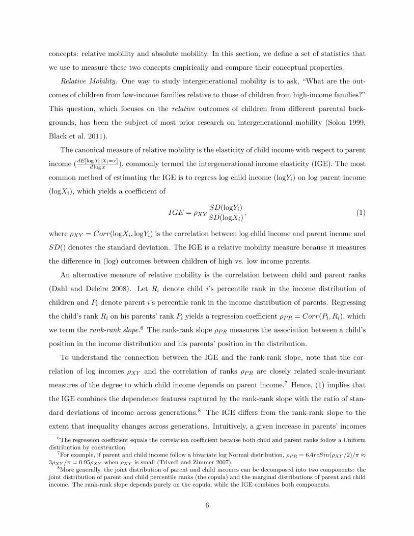
concepts: relative mobility and absolute mobility. In this section, we define a set of statistics that

we use to measure these two concepts empirically and compare their conceptual properties.

Relative Mobility. One way to study intergenerational mobility is to ask, “What are the out-

comes of children from low-income families relative to those of children from high-income families?”

This question, which focuses on the relative outcomes of children from different parental back-

grounds, has been the subject of most prior research on intergenerational mobility (Solon 1999,

Black et al. 2011).

The canonical measure of relative mobility is the elasticity of child income with respect to parent

income (dE[log Yi|Xi=x]d log x ), commonly termed the intergenerational income elasticity (IGE). The most

common method of estimating the IGE is to regress log child income (logYi) on log parent income

(logXi), which yields a coefficient of

IGE = ρXYSD(logYi)

SD(logXi), (1)

where ρXY = Corr(logXi, logYi) is the correlation between log child income and parent income and

SD() denotes the standard deviation. The IGE is a relative mobility measure because it measures

the difference in (log) outcomes between children of high vs. low income parents.

An alternative measure of relative mobility is the correlation between child and parent ranks

(Dahl and Deleire 2008). Let Ri denote child i’s percentile rank in the income distribution of

children and Pi denote parent i’s percentile rank in the income distribution of parents. Regressing

the child’s rank Ri on his parents’ rank Pi yields a regression coefficient ρPR = Corr(Pi, Ri), which

we term the rank-rank slope.6 The rank-rank slope ρPR measures the association between a child’s

position in the income distribution and his parents’ position in the distribution.

To understand the connection between the IGE and the rank-rank slope, note that the cor-

relation of log incomes ρXY and the correlation of ranks ρPR are closely related scale-invariant

measures of the degree to which child income depends on parent income.7 Hence, (1) implies that

the IGE combines the dependence features captured by the rank-rank slope with the ratio of stan-

dard deviations of income across generations.8 The IGE differs from the rank-rank slope to the

extent that inequality changes across generations. Intuitively, a given increase in parents’ incomes

6The regression coefficient equals the correlation coefficient because both child and parent ranks follow a Uniformdistribution by construction.

7For example, if parent and child income follow a bivariate log Normal distribution, ρPR = 6ArcSin(ρXY /2)/π ≈3ρXY /π = 0.95ρXY when ρXY is small (Trivedi and Zimmer 2007).

8More generally, the joint distribution of parent and child incomes can be decomposed into two components: thejoint distribution of parent and child percentile ranks (the copula) and the marginal distributions of parent and childincome. The rank-rank slope depends purely on the copula, while the IGE combines both components.

6

has a greater impact on the level of children’s incomes when inequality is greater among children

than parents.

We estimate both the IGE and the rank-rank slope to distinguish differences in mobility from

differences in inequality and to provide a comparison to the prior literature. However, we focus

primarily on rank-rank slopes because they prove to be much more robust across specifications and

are thus more suitable for comparisons across areas from a statistical perspective.

Absolute Mobility. A different way to measure intergenerational mobility is to ask, “What are

the outcomes of children from families of a given income level in absolute terms?” For example,

one may be interested in measuring the mean outcomes of children whose grow up in low-income

families. Absolute mobility may be of greater normative interest than relative mobility. Increases

in relative mobility (i.e., a lower IGE or rank-rank slope) could be undesirable if they are caused

by worse outcomes for the rich. In contrast, increases in absolute mobility at a given income

level, holding fixed absolute mobility at other income levels, unambiguously increase welfare if one

respects the Pareto principle (and if welfare depends purely on income).

We consider three statistical measures of absolute mobility. Our primary measure, which we

term absolute upward mobility, is the mean rank (in the national child income distribution) of

children whose parents are at the 25th percentile of the national parent income distribution.9 At

the national level, this statistic is mechanically related to the rank-rank slope and does not provide

any additional information about mobility.10 However, when we study small areas within the U.S.,

a child’s rank in the national income distribution is effectively an absolute outcome because incomes

in a given area have little impact on the national distribution.

The second measure we analyze is the probability of rising from the bottom quintile to the top

quintile of the income distribution (Corak and Heisz 1999, Hertz 2006), which can be interpreted as

a measure of the fraction of children who achieve the “American Dream.” Again, when the quintiles

are defined in the national income distribution, these transition probabilities can be interpreted as

measures of absolute outcomes in small areas. Our third measure is the probability that a child has

family income above the poverty line conditional on having parents at the 25th percentile. Because

the poverty line is defined in absolute dollar terms in the U.S., this statistic measures the fraction

9This measure is the analog of the rank-rank slope in terms of absolute mobility. The corresponding analog ofthe IGE is the mean log income of children whose parents are at the 25th percentile. We do not study this statisticbecause it is very sensitive to the treatment of zeros and small incomes.

10We show below that the rank-rank relationship is approximately linear. Because child and parent ranks eachhave a mean of 0.5 by construction in the national distribution, the mean rank of children with parents at percentilep is simply 0.5 + ρPR(p − 0.5). Conceptually, the slope is the only free parameter in the linear national rank-rankrelationship. Intuitively, if one child moves up in the income distribution in terms of ranks, another must come down.

7

of children who achieve a given absolute living standard.11

It is useful to analyze multiple measures of mobility because the appropriate measure of inter-

generational mobility depends upon one’s normative objective (Fields and Ok 1999). Fortunately,

we find that the patterns of spatial variation in absolute and relative mobility are very similar us-

ing alternative measures. In addition, we provide non-parametric transition matrices and marginal

distributions that allow readers to construct measures of mobility beyond those we consider here.

III Data

We use data from federal income tax records spanning 1996-2012. The data include both income

tax returns (1040 forms) and third-party information returns (e.g., W-2 forms), which give us

information on the earnings of those who do not file tax returns. We provide a detailed description

of how we construct our analysis sample starting from the raw population data in Online Appendix

A. Here, we briefly summarize the key variable and sample definitions. Note that in what follows,

the year always refers to the tax year (i.e., the calendar year in which the income is earned).

III.A Sample Definitions

Our base dataset of children consists of all individuals who (1) have a valid Social Security Number

or Individual Taxpayer Identification Number, (2) were born between 1980-1991, and (3) are U.S.

citizens as of 2013. We impose the citizenship requirement to exclude individuals who are likely to

have immigrated to the U.S. as adults, for whom we cannot measure parent income. We cannot

directly restrict the sample to individuals born in the U.S. because the database only records current

citizenship status.

We identify the parents of a child as the first tax filers (between 1996-2012) who claim the child

as a child dependent and were between the ages of 15 and 40 when the child was born. If the child is

first claimed by a single filer, the child is defined as having a single parent. For simplicity, we assign

each child a parent (or parents) permanently using this algorithm, regardless of any subsequent

changes in parents’ marital status or dependent claiming.12

11Another intuitive measure of upward mobility is the fraction of children whose income exceeds that of theirparents. This statistic turns out to be problematic for our application because we measure parent and child incomeat different ages and because it is very sensitive to differences in local income distributions.

1212% of children in our core sample are claimed as dependents by different individuals in subsequent years. Toensure that this potential measurement error in linking children to parents does not affect our findings, we show thatwe obtain similar estimates of mobility for the subset of children who are never claimed by other individuals (row 9of Online Appendix Table VII).

8

If parents never file a tax return, we cannot link them to their child. Although some low-income

individuals do not file tax returns in a given year, almost all parents file a tax return at some point

between 1996 and 2012 to obtain a tax refund on their withheld taxes and the Earned Income

Tax Credit (Cilke 1998). We are therefore able to identify parents for approximately 95% of the

children in the 1980-1991 birth cohorts. The fraction of children linked to parents drops sharply

prior to the 1980 birth cohort because our data begin in 1996 and many children begin to the leave

the household starting at age 17 (Online Appendix Table I). This is why we limit our analysis to

children born during or after 1980.

Our primary analysis sample, which we refer to as the core sample, includes all children in the

base dataset who (1) are born in the 1980-82 birth cohorts, (2) for whom we are able to identify

parents, and (3) whose mean parent income between 1996-2000 is strictly positive (which excludes

1.2% of children).13 For some robustness checks, we use the extended sample, which imposes

the same restrictions as the core sample, but includes all birth cohorts from 1980-1991. There

are approximately 10 million children in the core sample and 44 million children in the extended

sample.

Statistics of Income Sample. Because we can only reliably link children to parents starting

with the 1980 birth cohort in the population tax data, we can only measure earnings of children

up to age 32 (in 2012) in the full sample. To evaluate whether estimates of intergenerational

mobility would change significantly if earnings were measured at later ages, we supplement our

analysis using annual cross-sections of tax returns maintained by the Statistics of Income (SOI)

division of the Internal Revenue Service prior to 1996. The SOI cross-sections provide identifiers for

dependents claimed on tax forms starting in 1987, allowing us to link parents to children back to

the 1971 birth cohort using an algorithm analogous to that described above (see Online Appendix

A for further details). The SOI cross-sections are stratified random samples of tax returns with

a sampling probability that rises with income; using sampling weights, we can calculate statistics

representative of the national distribution. After linking parents to children in the SOI sample,

we use population tax data to obtain data on income for children and parents, using the same

definitions as in the core sample. There are approximately 63,000 children in the 1971-79 birth

cohorts in the SOI sample (Online Appendix Table II).

13We limit the sample to parents with positive income because parents who file a tax return (as required to linkthem to a child) yet have zero income are unlikely to be representative of individuals with zero income and thosewith negative income typically have large capital losses, which are a proxy for having significant wealth.

9

III.B Variable Definitions and Summary Statistics

In this section, we define the key variables we use to measure intergenerational mobility. We

measure all monetary variables in 2012 dollars, adjusting for inflation using the consumer price

index (CPI-U).

Parent Income. Following Lee and Solon (2009), our primary measure of parent income is total

pre-tax income at the household level, which we label parent family income. More precisely, in years

where a parent files a tax return, we define family income as Adjusted Gross Income (as reported on

the 1040 tax return) plus tax-exempt interest income and the non-taxable portion of Social Security

and Disability benefits. In years where a parent does not file a tax return, we define family income

as the sum of wage earnings (reported on form W-2), unemployment benefits (reported on form

1099-G), and gross social security and disability benefits (reported on form SSA-1099) for both

parents.14 In years where parents have no tax return and no information returns, family income is

coded as zero.15

Our baseline income measure includes labor earnings and capital income as well as unemploy-

ment insurance, social security, and disability benefits. It excludes non-taxable cash transfers such

as TANF and SSI, in-kind benefits such as food stamps, all refundable tax credits such as the

EITC, non-taxable pension contributions (e.g., to 401(k)’s), and any earned income not reported

to the IRS. Income is always measured prior to the deduction of individual income taxes and

employee-level payroll taxes.

In our baseline analysis, we average parents’ family income over the five years from 1996 to 2000

to obtain a proxy for parent lifetime income that is less affected by transitory fluctuations (Solon

1992). We use the earliest years in our sample to best reflect the economic resources of parents while

the children in our sample are growing up.16 We evaluate the robustness of our findings using data

14The database does not record W-2’s and other information returns prior to 1999, so non-filer’s income is codedas 0 prior to 1999. Assigning non-filing parents 0 income has little impact on our estimates because only 2.9% ofparents in our core sample do not file in each year prior to 1999 and most non-filers have very low W-2 income. Forinstance, in 2000, median W-2 income among non-filers was $29. Furthermore, we show below that defining parentincome based on data from 1999-2003 (when W-2 data are available) yields virtually identical estimates (Table I,row 5). Note that we never observe self-employment income for non-filers and therefore code it as zero; given thestrong incentives for individuals with children to file created by the EITC, most non-filers likely have very low levelsof self-employment income as well.

15Importantly, these observations are true zeros rather than missing data. Because the database covers all taxrecords, we know that these individuals have 0 taxable income.

16Formally, we define mean family income as the mother’s family income plus the father’s family income in eachyear from 1996 to 2000 divided by 10 (or divided by 5 if we only identify a single parent). For parents who donot change marital status, this is simply mean family income over the 5 year period. For parents who are marriedinitially and then divorce, this measure tracks the mean family incomes of the two divorced parents over time. Forparents who are single initially and then get married, this measure tracks individual income prior to marriage and

10

from other years and using a measure of individual parent income instead of family income. We

define individual income as the sum of individual W-2 wage earnings, UI benefits, SSDI payments,

and half of household self-employment income (see Online Appendix A for details).

Child Income. We define child family income in exactly the same way as parent family income.

In our baseline analysis, we average child family income over the last two years in our data (2011

and 2012), when children are in their early 30’s. We report results using alternative years to assess

the sensitivity of our findings. For children, we define household income based on current marital

status rather than marital status at a fixed point in time. Because family income varies with

marital status, we also report results using individual income measures for children, constructed in

the same way as for parents.

College Attendance. We define college attendance as an indicator for having one or more 1098-T

forms filed on one’s behalf when the individual is aged 18-21. Title IV institutions – all colleges and

universities as well as vocational schools and other post-secondary institutions eligible for federal

student aid – are required to file 1098-T forms that report tuition payments or scholarships received

for every student. Because the 1098-T forms are filed directly by colleges independent of whether

an individual files a tax return, we have complete records on college attendance for all children.

The 1098-T data are available from 1999-2012. Comparisons to other data sources indicate that

1098-T forms capture college enrollment quite accurately overall (Chetty, Friedman, and Rockoff

2014, Appendix B).17

College Quality. Using data from 1098-T forms, Chetty, Friedman, and Rockoff (2014 forthcom-

ing) construct an earnings-based index of “college quality” using the mean individual wage earnings

at age 31 of children born in 1979-80 based on the college they attended at age 20. Children who

do not attend college are included in a separate “no college” category in this index. We assign each

child in our sample a value of this college quality index based on the college in which they were

enrolled at age 20. We then convert this dollar index to percentile ranks within each birth cohort.

The children in the no-college group, who constitute roughly 54% of our core sample, all have the

same value of the college quality index. Breaking ties at the mean, we assign all of these children

total family income (including the new spouse’s income) after marriage. These household measures of income increasewith marriage and naturally do not account for cohabitation; to ensure that these features do not generate bias, weassess the robustness of our results to using individual measures of income.

17Colleges are not required to file 1098-T forms for students whose qualified tuition and related expenses arewaived or paid entirely with scholarships or grants. However, the forms are frequently available even for such cases,presumably because of automated reporting to the IRS by universities. Approximately 6% of 1098-T forms aremissing from 2000-2003 because the database contains no 1098-T forms for some small colleges in these years. Toverify that this does not affect our results, we confirm that our estimates of college attendance by parent incomegradients are very similar for later birth cohorts (not reported).

11

a college quality rank of approximately 54/2 = 27.18

Teenage Birth. We define a woman as having a teenage birth if she ever claims a dependent

who was born while she was between the ages of 13 and 19. This measure is an imperfect proxy

for having a teenage birth because it only covers children who are claimed as dependents by their

mothers. Nevertheless, the aggregate level and spatial pattern of teenage births in our data are

closely aligned with estimates based on the American Community Survey.19

Summary Statistics. Online Appendix Table III reports summary statistics for the core sample.

Median parent family income is $60,129 (in 2012 dollars). Among the 30.6% of children matched to

single parents, 72.0% are matched to a female parent. Children in our core sample have a median

family income of $34,975 when they are approximately 30 years old. 6.1% of children have zero

income in both 2011 and 2012. 58.9% are enrolled in a college at some point between the ages of

18 and 21 and 15.8% of women have a teenage birth.

In Online Appendix B and Appendix Table IV, we show that the total cohort size, labor

force participation rate, distribution of child income, and other demographic characteristics of our

core sample line up closely with corresponding estimates in the Current Population Survey and

American Community Survey. This confirms that our sample covers roughly the same nationally

representative population as previous survey-based research.

IV National Statistics

We begin our empirical analysis by characterizing the relationship between parent and child income

at the national level. We first present a set of baseline estimates of relative mobility and then

evaluate the robustness of our estimates to alternative sample and income definitions.20

IV.A Baseline Estimates

In our baseline analysis, we use the core sample (1980-82 birth cohorts) and measure parent income

as mean family income from 1996-2000 and child income as mean family income in 2011-12, when

18The exact value varies across cohorts. For example, in the 1980 birth cohort, 55.1% of children do not attendcollege. We assign these children a rank of 55.1/2+0.02=27.7% because 0.2% of children in the 1980 birth cohortattend colleges whose mean earnings are below the mean earnings of those not in college.

1915.8% of women in our core sample have teenage births; the corresponding number is 14.6% in the 2003 ACS.The unweighted correlation between state-level teenage birth rates in the tax data and the ACS is 0.80.

20We do not present estimates of absolute mobility at the national level because absolute mobility in terms ofpercentile ranks is mechanically related to relative mobility at the national level (see Section II). While one cancompute measures of absolute mobility at the national level based on mean incomes (e.g., the mean income ofchildren whose parents are at the 25th percentile), there is no natural benchmark for such a statistic as it has notbeen computed in other countries or time periods.

12

children are approximately 30 years old. Figure Ia presents a binned scatter plot of the mean

family income of children versus the mean family income of their parents. To construct this figure,

we divide the horizontal axis into 100 equal-sized (percentile) bins and plot mean child income

vs. mean parent income in each bin.21 This binned scatter plot provides a non-parametric repre-

sentation of the conditional expectation of child income given parent income, E[Yi|Xi = x]. The

regression coefficients and standard errors reported in this and all subsequent binned scatter plots

are estimated on the underlying microdata using OLS regressions.

The conditional expectation of children’s income given parents’ income is strongly concave.

Below the 90th percentile of parent income, a $1 increase in parent family income is associated

with a 33.5 cent increase in average child family income. In contrast, between the 90th and 99th

percentile, a $1 increase in parent income is associated with only a 7.6 cent increase in child income.

Log-Log Intergenerational Elasticity Estimates. Partly motivated by the non-linearity of the re-

lationship in Figure Ia, the canonical approach to characterizing the joint distribution of child and

parent income is to regress the log of child income on the log of parent income (as discussed in Sec-

tion II), excluding children with zero income. This regression yields an estimated intergenerational

elasticity (IGE) of 0.344, as shown in the first column of row 1 of Table I.

Unfortunately, this estimate turns out to be quite sensitive to changes in the regression speci-

fications for two reasons, illustrated in Figure Ib. First, the relationship between log child income

and log parent income is highly non-linear, consistent with the findings of Corak and Heisz (1999)

in Canadian tax data. This is illustrated in the series in circles in Figure Ib, which plots mean log

child income vs. mean log family income by percentile bin, constructed using the same method as

Figure Ia. Because of this non-linearity, the IGE is sensitive to the point of measurement in the

income distribution. For example, restricting the sample to observations between the 10th and 90th

percentile of parent income (denoted by the vertical dashed lines in the graph) yields a considerably

higher IGE estimate of 0.452.

Second, the log-log specification discards observations with zero income. The series in triangles

in Figure Ib plots the fraction of children with zero income by parental income bin. This fraction

varies from 17% among the poorest families to 3% among the richest families. Dropping children

with zero income therefore overstates the degree of intergenerational mobility. The way in which

these zeros are treated can change the IGE dramatically. For instance, including the zeros by

21For scaling purposes, we exclude the top bin (parents in the top 1%) in this figure only; mean parent income inthis bin is $1,408,760 and mean child income is $113,846.

13

assigning those with zero income an income of $1 (so that the log of their income is zero) raises

the estimated IGE to 0.618, as shown in row 2 of Table I. If instead we treat those with 0 income

as having an income of $1,000, the estimated IGE becomes 0.413. These exercises show that small

differences in the way children’s income is measured at the bottom of the distribution can produce

substantial variation in IGE estimates.

Columns 2-7 in Table I replicate the baseline specification in Column 1 for alternative subsam-

ples analyzed in the prior literature. Columns 2-5 split the sample by the child’s gender and the

parents’ marital status in the year they first claim the child. Column 6 replicates Column 1 for

the extended sample of 1980-85 birth cohorts. Column 7 restricts the sample to children whose

mothers are between the ages of 24-28 and fathers are between 26-30 (a five year window around the

median age of birth). This column eliminates variation in parent income correlated with differences

in parent age at child birth and restricts the sample to parents who are less than 50 years old when

we measure their incomes (for children born in 1980). Across these subsamples, the IGE estimates

range from 0.264 (for children of single parents, excluding children with zero income) to 0.697 (for

male children, recoding zeroes to $1).

The IGE is unstable because the income distribution is not well approximated by a bivariate

Log-Normal distribution, a result that was not apparent in smaller samples used in prior work.

This makes it difficult to obtain reliable comparisons of mobility across samples or geographical

areas using the IGE. For example, income measures in survey data are typically top-coded and

sometimes include transfers and other sources of income that increase incomes at the bottom of

the distribution, which may lead to larger IGE estimates than those obtained in administrative

datasets such as the one used here.

In a recent paper, Mitnik et al. (2014) propose a new measure of the IGE, the elasticity of

expected child income with respect to parent income (d logE[Yi|Xi=x]d log x ), which they show is more

robust to the treatment of small incomes. In large samples, one can estimate this parameter by

regressing the log of mean child income in each percentile bin (plotted in Figure Ia) on the log of

mean parent income in each bin. In Online Appendix C, we show that Mitnik et al.’s statistic can

be interpreted as a dollar-weighted average of elasticities (placing greater weight on high income

children), whereas the traditional IGE weights all individuals with positive income equally. These

two parameters need not coincide in general and the “correct” parameter depends upon the policy

question one seeks to answer. However, it turns out that in our data, the Mitnik et al. dollar-

weighted IGE estimate is 0.335, very similar to our baseline IGE estimate of 0.344 when excluding

14

children with zero income (Online Appendix Figure Ia).22

In another recent study, Clark (2014) argues that traditional estimates of the IGE understate

the persistence of status across generations because they are attenuated by fluctuations in realized

individual incomes across generations. To resolve this problem, Clark estimates the IGE based on

surname-level means of income in each generation and obtains a central IGE estimate of 0.8, much

larger than that in prior studies. In our data, estimates of mobility based on surname means are

similar to our baseline estimates based on individual income data (Online Appendix Table V). One

reason that Clark (2014) may obtain larger estimates of intergenerational persistence is that his

focus on distinctive surnames partly identifies the degree of convergence in income between racial

or ethnic groups (Borjas 1992) rather than across individuals (see Online Appendix D for further

details).23

Rank-Rank Estimates. Next, we present estimates of the rank-rank slope, the second measure

of relative mobility discussed in Section II. We measure the percentile rank of parents Pi based

on their positions in the distribution of parent incomes in the core sample. Similarly, we define

children’s percentile ranks Ri based on their positions in the distribution of child incomes within

their birth cohorts. Importantly, this definition allows us to include zeros in child income.24 Unless

otherwise noted, we hold the definition of these ranks fixed based on positions in the aggregate

distribution, even when analyzing subgroups.

Figure IIa presents a binned scatter plot of the mean percentile rank of children E[Ri|Pi = p]

vs. their parents’ percentile rank p. The conditional expectation of a child’s rank given his parents’

rank is almost perfectly linear. Using an OLS regression, we estimate that a one percentage point

(pp) increase in parent rank is associated with a 0.341 pp increase in the child’s mean rank, as

reported in row 4 of Table I. The rank-rank slope estimates are generally quite similar across

subsamples, as shown in Columns 2-7 of Table I.

Figure IIb compares the rank-rank relationship in the U.S. with analogous estimates for Den-

mark constructed using data from Boserup, Kopczuk and Kreiner (2013) and estimates for Canada

22Mitnik et al. (2014) find larger estimates of the dollar-weighted IGE in their sample of tax returns. A usefuldirection for further work would be to understand why the two samples yield different IGE estimates.

23For example, Clark (2014, page 60, Figure 3.10) compares the outcomes of individuals with the surname “Katz”(a predominantly Jewish name) vs. “Washington” (a predominantly black name). This comparison generates animplied IGE close to 1, which partly reflects the fact that the black-white income gap has changed very little overthe past few decades. Estimates of the IGE based on individual-level data (or pooling all surnames) are much lowerbecause there is much more social mobility within racial groups.

24In the case of ties, we define the rank as the mean rank for the individuals in that group. For example, if 10%of a birth cohort has zero income, all children with zero income would receive a percentile rank of 5.

15

constructed from the decile transition matrix reported by Corak and Heisz (1999).25 The relation-

ship between child and parent ranks is nearly linear in Denmark and Canada as well, suggesting

that the rank-rank specification provides a good summary of mobility across diverse environments.

The rank-rank slope is 0.180 in Denmark and 0.174 in Canada, nearly half that in the U.S.

Importantly, the smaller rank-rank slopes in Denmark and Canada do not necessarily mean that

children from low-income families in these countries do better than those in the U.S. in absolute

terms. It could be that children of high-income parents in Denmark and Canada have worse

outcomes than children of high-income parents in the U.S. One cannot distinguish between these

possibilities because the ranks are defined within each country. One advantage of the within-

U.S. CZ-level analysis implemented below is that it naturally allows us to study both relative and

absolute outcomes by analyzing children’s performance on a fixed national scale.

Transition Matrices. Table II presents a quintile transition matrix: the probability that a child

is in quintile m of the child income distribution conditional on his parent being in quintile n of the

parent income distribution. One statistic of particular interest in this matrix is the probability of

moving from the bottom quintile to the top quintile, a simple measure of success that we return to

below. This probability is 7.5% in the U.S., compared with 11.7% in Denmark (Boserup, Kopczuk

and Kreiner 2013) and 13.4% in Canada (Corak and Heisz 1999). In this sense, the chances of

achieving the “American Dream” are considerably higher for children in Denmark and Canada

than those in the U.S.

In Online Data Table I, we report a 100 x 100 percentile-level transition matrix for the U.S.

Using this matrix and the marginal distributions for child and parent income in Online Data Table

II, one can construct any mobility statistic of interest for the U.S. population.26

IV.B Robustness of Baseline Estimates

We now evaluate the robustness of our estimates of intergenerational mobility to alternative speci-

fications. We begin by evaluating two potential sources of bias emphasized in prior work: lifecycle

bias and attenuation bias.

25Both the Danish and Canadian studies use administrative earnings information for large samples as we do here.The Danish sample, which was constructed to match the analysis sample in this paper as closely as possible, consistsof children in the 1980-81 birth cohorts and measures child income based on mean income between 2009-11. Childincome in the Danish sample is measured at the individual level and parents’ income is the mean of the two biologicalparents’ income from 1997-1999, irrespective of their marital status. The Canadian sample is less comparable to oursample, as it consists of male children in the 1963-66 birth cohorts and studies the link between their mean earningsfrom 1993-95 and their fathers’ mean earnings from 1978-82.

26All of the online data tables are available at http://www.equality-of-opportunity.org/index.php/data.

16

Lifecycle Bias. Prior research has shown that measuring children’s income at early ages can

understate intergenerational persistence in lifetime income because children with high lifetime in-

comes have steeper earnings profiles when they are young (Haider and Solon, 2006, Grawe, 2006,

Solon 1999). To evaluate whether our baseline estimates suffer from such lifecycle bias, Figure IIIa

plots estimates of the rank-rank slope by the age at which the child’s income is measured. We

construct the series in circles by measuring children’s income as mean family income in 2011-2012

and parent income as mean family income between 1996-2000, as in our baseline analysis. We

then replicate the OLS regression of child income rank on parent income rank for each birth cohort

between 1980-1990. For children in the 1980 birth cohort, we measure earnings in 2011-12 at age

31-32 (denoted by 32 in the figure); for the 1990 cohort, we measure earnings at age 21-22.27 The

rank-rank slope rises very steeply in the early 20’s as children enter the labor force, but stabilizes

around age 30. It increases by 2.1% from age 30 to 31 and 0.2% from age 31 to 32.

To obtain estimates beyond age 32, we use the SOI 0.1% random sample described in Section

III.A, which contains data back to the 1971 birth cohort. The series in triangles in Figure IIIa

replicates the analysis above within the SOI sample, using sampling weights to recover estimates

representative of the population. The estimates in the SOI sample are very similar to those in

the full population prior to age 32. After age 32, the estimates remain roughly constant. These

findings indicate that rank-rank correlations exhibit little lifecycle bias provided that child income

is measured after age 30, as in our baseline definition.

We also find that estimates of the IGE using the traditional log-log specification (limiting the

sample between the 10th and 90th percentiles of the parent income distribution) stabilize around

age 30, as shown in Online Appendix Figure IIa. In the population data, the IGE estimate is a

strictly concave function of age and rises by only 1.7% from age 31 to 32. The SOI 0.1% sample

exhibits a similar, albeit noisier, pattern.

An analogous lifecycle bias can arise if parent income is measured at very old or young ages. In

Online Appendix Figure IIb we plot the rank-rank slope using the core sample, varying the 5-year

window used to measure parent income from a starting year of 1996 (when mothers are 41 years

old on average) to 2010 (when mothers are 55 years old). The rank-rank estimates exhibit virtually

no variation with the age of parent income measurement within this range.

A closely related concern is that parent income at earlier ages might matter more for children’s

27We obtain very similar results if we instead track a single cohort and vary age by measuring earnings in differentcalendar years.

17

outcomes, e.g. if resources in early childhood are relevant for child development (e.g., Heckman

2006, Duncan, Ziol-Guest and Kalil 2010). While we cannot measure parent income before age 14

for children in our core sample, we can measure parent income at earlier ages for later birth cohorts.

In Chetty et al. (2014), we use data from the 1993 birth cohort and regress an indicator for college

attendance at age 19 on parent income rank in each year from 1996 to 2012. We reproduce the

coefficients from those regressions in Online Appendix Figure IIc. The relationship between college

attendance rates and parent income rank is virtually constant when children are between ages 3 and

19. Once again, this result indicates that the point at which parent income is measured (provided

parents are between ages 30-55) does not significantly affect intergenerational associations, at least

in administrative earnings records.28

Attenuation Bias. Income in a single year is a noisy measure of lifetime income, which atten-

uates estimates of intergenerational persistence (Solon (1992)). To evaluate whether our baseline

estimates suffer from such attenuation bias, Figure IIIb plots estimates of the rank-rank slope,

varying the number of years used to calculate mean parent family income. In this figure, we plot

the slope from an OLS regression of child rank on parent rank (as in Row 4, Column 1 of Table

I), varying the number of years used to calculate mean parent income from one (1996 only) to 17

(1996-2012). The rank-rank slope based on five years of data (0.341) is 6.6% larger than the slope

based on one year of parent income (0.320). Solon (1992) finds a 33% increase in the IGE (from

0.3 to 0.4) when using a five-year average instead of one year of data in the PSID. We find less

attenuation bias for three reasons: (1) income is measured with less error in the tax data than in

the PSID, (2) we use family income measures rather than individual income, which fluctuates more

across years, and (3) we use a rank-rank specification rather than a log-log specification, which is

more sensitive to income fluctuations at the bottom of the distribution.

Mazumder (2005) reports that even five-year averages of parent income yield attenuated es-

timates of intergenerational persistence relative to longer time averages. Contrary to this result,

we find that the rank-rank slope is virtually unchanged by adding more years of data beyond five

years: the estimated slope using 15 years of data to measure parent income (0.350) is only 2.8%

larger than the baseline slope of 0.341 using 5 years of data. We believe our results differ because

we directly measure parent income, whereas Mazumder imputes parent income based on race and

28While we cannot measure income before the year in which children turn 3, the fact that the college-incomegradient is not declining from ages 3-19 makes it unlikely that the gradient is significantly larger prior to age 2.Parent income ranks in year t have a correlation of 0.91 with parent income ranks in year t + 1, 0.77 in year t + 5,and 0.65 in year t+ 15. The decay in this autocorrelation would generate a decreasing slope in the gradient in OnlineAppendix Figure IIc if there were a discontinuous jump in the gradient prior to age 2.

18

education for up to 60% of the observations in his sample, with a higher imputation rate when

measuring parent income using more years (see Online Appendix E for further details). Such im-

putations are analogous to instrumenting for income with race and education, which is known to

yield upward-biased estimates of intergenerational persistence (Solon 1992).

We analyze the impact of varying the number of years used to measure the child’s income in

Online Appendix Figure IId. The rank-rank slope increases very little when increasing the number

of years used to compute child family income, with no detectable change once one averages over

at least two years, as in our baseline measure. An ancillary implication of this result is that our

estimates of intergenerational mobility are not sensitive to the calendar year in which we measure

children’s incomes. This finding is consistent with the results of Chetty et al. (2014), who show that

estimates of intergenerational mobility do not vary significantly across birth cohorts when income

is measured at a fixed age.

Alternative Income Definitions. In rows 5-8 of Table I, we explore the robustness of the baseline

rank-rank estimate to alternative definitions of child and parent income. In row 5, we verify that the

missing W-2 data from 1996-1998 does not create significant bias by defining parent income as mean

income from 1999-2003. The rank-rank estimates are virtually unchanged with this redefinition.

In row 6, we define the parent’s rank based on the individual income of the parent with higher

mean income from 1999-2003.29 This specification eliminates the mechanical variation in family

income driven by the number of parents in the household, which could overstate the persistence of

income across generations if parent marital status has a direct effect of children’s outcomes. The

rank-rank correlation falls by approximately 10%, from 0.341 to 0.312 when we use top parent

income. The impact of using individual parent income instead of family income is modest because

(1) most of the variation in parent income across households is not due to differences in marital

status and (2) the mean ranks of children with married parents are only 4.6 percentile points higher

than those with single parents.

Next, we consider alternative income definitions for the children. Here, one concern is that

children of higher income parents may be more likely to marry, again exaggerating the observed

persistence in family income relative to individual income. Using individual income to measure

the child’s rank has differential impacts by the child’s gender, consistent with Chadwick and Solon

29We use 1999-2003 income here because we cannot allocate earnings across spouses before 1999, as W-2 forms areavailable starting only in 1999. Note that top income rank differs from family income rank even for single parentsbecause some individuals get married in subsequent years and because these individuals are ranked relative to thepopulation, not relative to other single individuals.

19

(2002). For male children, using individual income instead of family income reduces the rank-rank

correlation from 0.336 in the baseline specification to 0.317, a 6% reduction. For female children,

using individual income reduces the rank-rank correlation from 0.346 to 0.257, a 26% reduction.

The change may be larger for women because women from high income families tend to marry

high-income men and may choose not to work.

Finally, in row 8 of Table I, we define a measure of child income that excludes capital and

other non-labor income using the sum of individual wage earnings, UI benefits, SSDI benefits,

and Schedule C self-employment income. We divide self-employment income by two for married

individuals. This individual earnings measure also yields virtually identical estimates of the rank-

rank slope.

IV.C Intermediate Outcomes: College Attendance and Teenage Birth

We supplement our analysis of intergenerational income mobility by studying the relationship

between parent income and two intermediate outcomes for children: college attendance and teenage

birth.

The series in circles in Figure IVa presents a binned scatter plot of the college attendance rate of

children vs. the percentile rank of parent family income using the core sample. College attendance

is defined as attending college in one or more years between the ages 18 and 21. The relationship

between college attendance rates and parental income rank is again virtually linear, with a slope

of 0.675. That is, moving from the lowest-income to highest-income parents increases the college

attendance rate by 67.5 percentage points, similar to the estimates reported by Bailey and Dynarski

(2011) using survey data.

The series in triangles in Figure IVa plots college quality ranks vs. parent ranks. We define a

child’s college quality rank based on the mean earnings at age 30 of students who attended each

college at age 20. The 54% of children who do not attend college at age 20 are included in this

analysis and are assigned the mean rank for the non-college group, which is approximately 54/2 =

27 (see Section III.B for details). The relationship between college quality rank and parent income

rank is convex because most children from low-income families do not attend college and hence

increases in parent income have little impact on college quality rank at the bottom. To account for

this non-linearity, we regress college quality ranks on a quadratic function of parent income rank

and define the gradient in college quality as the difference in the predicted college quality rank for

children with parents at the 75th percentile and children with parents at the 25th percentile. The

20

P25-75 gap in college quality ranks is 19.1 percentiles in our core sample.

Figure IVb plots teenage birth rates for female children vs. parent income ranks. Teenage birth

is defined (for females only) as having a child when the mother is aged 13-19. There is a 29.8

percentage point gap in teenage birth rates between children from the highest- and lowest-income

families.

These correlations between intermediate outcomes and parent income ranks do not vary sig-

nificantly across subsamples or birth cohorts, as shown in rows 9-11 of Table I. The strength of

these correlations indicates that much of the divergence between children from low vs. high income

families emerges well before they enter the labor market, consistent with the findings of prior work

(e.g., Neal and Johnson 1996, Cameron and Heckman 2001, Bhattacharya and Mazumder 2011).

V Spatial Variation in Mobility

We now turn to our central goal of characterizing the variation in intergenerational mobility across

areas within the U.S. We begin by defining measures of geographic location. We then present

estimates of relative and absolute mobility by area and assess the robustness of these estimates to

alternative specifications.

V.A Geographical Units

To characterize the variation in children’s outcomes across areas, one must first partition the U.S.

into a set of geographical areas in which children grow up. One way to conceptualize the choice of

a geographical partition is using a hierarchical model in which children’s outcomes depend upon

conditions in their immediate neighborhood (e.g., peers or resources in their city block), local

community (e.g., the quality of schools in their county), and broader metro area (e.g., local labor

market conditions). To fully characterize the geography of intergenerational mobility, one would

ideally estimate all of the components of such a hierarchical model.

As a first step toward this goal, we characterize intergenerational mobility at the level of com-

muting zones (CZs). CZs are aggregations of counties based on commuting patterns in the 1990

Census constructed by Tolbert and Sizer (1996) and introduced to the economics literature by Dorn

(2009). Since CZs are designed to span the area in which people live and work, they provide a

natural starting point as the coarsest partition of areas. CZs are similar to metropolitan statistical

areas (MSA), but unlike MSAs, they cover the entire U.S., including rural areas. There are 741

CZs in the U.S.; on average, each CZ contains 4 counties and has a population of 380,000. See

21

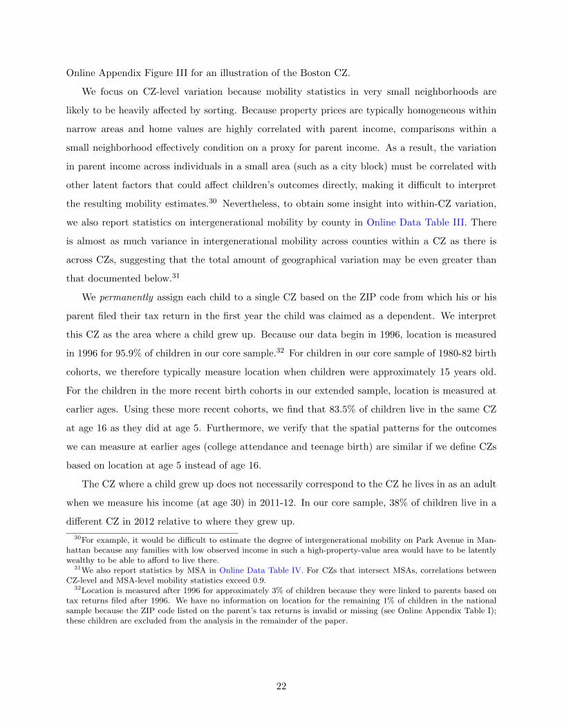
Online Appendix Figure III for an illustration of the Boston CZ.

We focus on CZ-level variation because mobility statistics in very small neighborhoods are

likely to be heavily affected by sorting. Because property prices are typically homogeneous within

narrow areas and home values are highly correlated with parent income, comparisons within a

small neighborhood effectively condition on a proxy for parent income. As a result, the variation

in parent income across individuals in a small area (such as a city block) must be correlated with

other latent factors that could affect children’s outcomes directly, making it difficult to interpret

the resulting mobility estimates.30 Nevertheless, to obtain some insight into within-CZ variation,

we also report statistics on intergenerational mobility by county in Online Data Table III. There

is almost as much variance in intergenerational mobility across counties within a CZ as there is

across CZs, suggesting that the total amount of geographical variation may be even greater than

that documented below.31

We permanently assign each child to a single CZ based on the ZIP code from which his or his

parent filed their tax return in the first year the child was claimed as a dependent. We interpret

this CZ as the area where a child grew up. Because our data begin in 1996, location is measured

in 1996 for 95.9% of children in our core sample.32 For children in our core sample of 1980-82 birth

cohorts, we therefore typically measure location when children were approximately 15 years old.

For the children in the more recent birth cohorts in our extended sample, location is measured at

earlier ages. Using these more recent cohorts, we find that 83.5% of children live in the same CZ

at age 16 as they did at age 5. Furthermore, we verify that the spatial patterns for the outcomes

we can measure at earlier ages (college attendance and teenage birth) are similar if we define CZs

based on location at age 5 instead of age 16.

The CZ where a child grew up does not necessarily correspond to the CZ he lives in as an adult

when we measure his income (at age 30) in 2011-12. In our core sample, 38% of children live in a

different CZ in 2012 relative to where they grew up.

30For example, it would be difficult to estimate the degree of intergenerational mobility on Park Avenue in Man-hattan because any families with low observed income in such a high-property-value area would have to be latentlywealthy to be able to afford to live there.

31We also report statistics by MSA in Online Data Table IV. For CZs that intersect MSAs, correlations betweenCZ-level and MSA-level mobility statistics exceed 0.9.

32Location is measured after 1996 for approximately 3% of children because they were linked to parents based ontax returns filed after 1996. We have no information on location for the remaining 1% of children in the nationalsample because the ZIP code listed on the parent’s tax returns is invalid or missing (see Online Appendix Table I);these children are excluded from the analysis in the remainder of the paper.

22

V.B Measures of Relative and Absolute Mobility

In our baseline analysis, we measure mobility at the CZ level using the core sample (1980-82 birth

cohorts) and the definitions of parent and child family income described in III.B. Importantly,

we continue to rank both children and parents based on their positions in the national income

distribution (rather than the distribution within their CZ).

We begin by examining the rank-rank relationship in selected CZs. Figure Va presents a binned

scatter plot of the mean child rank vs. parent rank for children who grew up in the Salt Lake City,

UT (circles) or Charlotte, NC (triangles) commuting zones. The rank-rank relationship is virtually

linear in both of these CZs. The linearity of the rank-rank relationship is a remarkably robust

property across CZs, as illustrated for the 20 largest CZs in Online Appendix Figure IV.

Exploiting this approximate linearity, we summarize the conditional expectation of a child’s

rank given his parents’ rank in each CZ using two parameters: a slope and an intercept. Let Ric

denote the national income rank (among children in his birth cohort) of child i who grew up in

CZ c. Similarly, let Pic denote his parent’s rank in the income distribution of parents in the core

sample. We estimate the slope and intercept of the rank-rank relationship in CZ c by regressing

child rank on parent rank:

Ric = αc + βcPic + εic (2)

The slope of the rank-rank relationship (βc) in (2) measures degree of relative mobility in CZ c, as

defined in Section II. In Salt Lake City, βc = 0.264.33 The difference between the expected ranks of

children born to parents at the top and bottom of the income distribution is r100,c−r0,c = 100×βc =

26.4 in Salt Lake City. There is much less relative mobility (i.e., much greater persistence of income

across generations) in Charlotte, where r100 − r0 = 39.7.

Following the discussion in Section II, we define absolute mobility at percentile p in CZ c as the

expected rank of a child who grew up in CZ c with parents who have a national income rank of p:

rpc = αc + βcp. (3)

We focus much of our analysis on average absolute mobility for children from families with below-

median parent income in the national distribution (E [Ric|Pic < 50]), which we term absolute upward

mobility.34 Because the rank-rank relationship is linear, the average rank of children with below-

33We always measure percentile ranks on a 0-100 scale and slopes on a 0-1 scale, so αc ranges from 0-100 and βcranges from 0 to 1 in (3).

34We integrate over the national parent income distribution rather than the local distribution when definingE [Ric|Pic < 50] to ensure that our cross-CZ comparisons are not affected by differences in local income distributions.

23

median parent income equals the average rank of children with parents at the 25th percentile in

the national distribution (r25,c = αc + 25βc), illustrated by the dashed vertical line in Figure Va.

Absolute upward mobility is r25 = 46.2 in Salt Lake City, compared with r25 = 35.8 in Charlotte.

That is, among families earning $28,800 – the 25th percentile of the national parent family income

distribution – children who grew up in Salt Lake City are on average 10 percentile points higher in

their birth cohort’s income distribution at age 30 than children who grew up in Charlotte.

Absolute mobility is higher in Salt Lake City not just for below-median families, but at all

percentiles p of the parent income distribution. The gap in absolute outcomes is largest at the

bottom of the income distribution and nearly zero at the top. Hence, the greater relative mobility

in this particular comparison comes purely from better absolute outcomes at the bottom of the

distribution rather than worse outcomes at the top. Of course, this is not always the case. Figure Vb

shows that San Francisco has substantially higher relative mobility than Chicago: r100 − r0 = 25.0

in San Francisco vs. r100 − r0 = 39.3 in Chicago. But part of the greater relative mobility in

San Francisco comes from worse outcomes for children from high-income families. Below the 60th

percentile, children in San Francisco have better outcomes than those in Chicago; above the 60th

percentile, the reverse is true.

The comparisons in Figure V illustrate the importance of measuring both relative and absolute

mobility. Any social welfare function based on mean income ranks that respects the Pareto principle

would rate Salt Lake City above Charlotte. But normative comparisons of San Francisco and

Chicago depend on the weight one puts on relative vs. absolute mobility (or, equivalently, on the

weights one places on absolute mobility at each percentile p).

V.C Baseline Estimates by CZ

We estimate (2) using OLS to calculate absolute upward mobility (r25,c = αc + 25βc) and relative

mobility (βc) by CZ. The estimates for each CZ are reported in Online Data Table V.

Absolute Upward Mobility. Figure VIa presents a heat map of absolute upward mobility. We

construct this map by dividing CZs into deciles based on their estimated value of r25,c. Lighter

colors represent deciles with higher levels of r25,c.35 Upward mobility varies significantly across

We focus on the absolute outcomes of children from low-income families both because the outcomes of disadvantagedyouth are a central focus of policy interest and because there is more variation across areas in the outcomes ofchildren from low-income families than those from high-income families, as we show in Figure VII below. However,the CZ-level statistics in Online Data Tables V and VI can be used to analyze spatial variation in the outcomes ofchildren from high-income families.

35We cannot estimate mobility for 32 CZs in which we have fewer than 250 children in the core sample, shown bythe cross-hatched areas in the maps in Figure VI. These CZs account for less than 0.05% of the U.S. population in

24

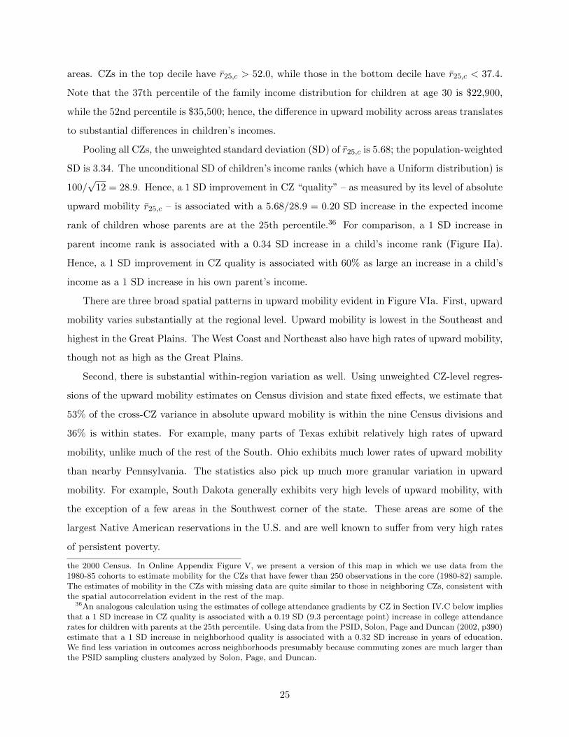
areas. CZs in the top decile have r25,c > 52.0, while those in the bottom decile have r25,c < 37.4.

Note that the 37th percentile of the family income distribution for children at age 30 is $22,900,

while the 52nd percentile is $35,500; hence, the difference in upward mobility across areas translates

to substantial differences in children’s incomes.

Pooling all CZs, the unweighted standard deviation (SD) of r25,c is 5.68; the population-weighted

SD is 3.34. The unconditional SD of children’s income ranks (which have a Uniform distribution) is

100/√

12 = 28.9. Hence, a 1 SD improvement in CZ “quality” – as measured by its level of absolute

upward mobility r25,c – is associated with a 5.68/28.9 = 0.20 SD increase in the expected income

rank of children whose parents are at the 25th percentile.36 For comparison, a 1 SD increase in

parent income rank is associated with a 0.34 SD increase in a child’s income rank (Figure IIa).

Hence, a 1 SD improvement in CZ quality is associated with 60% as large an increase in a child’s

income as a 1 SD increase in his own parent’s income.

There are three broad spatial patterns in upward mobility evident in Figure VIa. First, upward

mobility varies substantially at the regional level. Upward mobility is lowest in the Southeast and

highest in the Great Plains. The West Coast and Northeast also have high rates of upward mobility,

though not as high as the Great Plains.

Second, there is substantial within-region variation as well. Using unweighted CZ-level regres-

sions of the upward mobility estimates on Census division and state fixed effects, we estimate that

53% of the cross-CZ variance in absolute upward mobility is within the nine Census divisions and

36% is within states. For example, many parts of Texas exhibit relatively high rates of upward

mobility, unlike much of the rest of the South. Ohio exhibits much lower rates of upward mobility

than nearby Pennsylvania. The statistics also pick up much more granular variation in upward

mobility. For example, South Dakota generally exhibits very high levels of upward mobility, with

the exception of a few areas in the Southwest corner of the state. These areas are some of the

largest Native American reservations in the U.S. and are well known to suffer from very high rates

of persistent poverty.

the 2000 Census. In Online Appendix Figure V, we present a version of this map in which we use data from the1980-85 cohorts to estimate mobility for the CZs that have fewer than 250 observations in the core (1980-82) sample.The estimates of mobility in the CZs with missing data are quite similar to those in neighboring CZs, consistent withthe spatial autocorrelation evident in the rest of the map.

36An analogous calculation using the estimates of college attendance gradients by CZ in Section IV.C below impliesthat a 1 SD increase in CZ quality is associated with a 0.19 SD (9.3 percentage point) increase in college attendancerates for children with parents at the 25th percentile. Using data from the PSID, Solon, Page and Duncan (2002, p390)estimate that a 1 SD increase in neighborhood quality is associated with a 0.32 SD increase in years of education.We find less variation in outcomes across neighborhoods presumably because commuting zones are much larger thanthe PSID sampling clusters analyzed by Solon, Page, and Duncan.

25

The third generic pattern is that urban areas tend to exhibit lower levels of intergenerational

mobility than rural areas on average. For instance, children from low-income families who grow

up in the Chicago area have significantly lower incomes at age 30 than those who grow up in rural

areas in Illinois. On average, urban areas – which we define as CZs that intersect MSAs – have

upward mobility of r25,c = 41.7, while rural areas have r25,c = 45.8. In interpreting this comparison,

it is important to recall that our definition of geography is based on where children grew up, not

where they live as adults. 44.6% of children who grow up in rural areas live in urban areas at age

30. Among those who rose from the bottom quintile of the national income distribution to the top

quintile, 55.2% of children who grew up in rural areas live in urban areas at age 30.

Table III shows statistics on intergenerational mobility for the 50 largest CZs by population.

Among these cities, absolute upward mobility ranges from 46.2 in the Salt Lake City area to 35.8

in Charlotte (Column 4). There is considerable variation even between nearby cities: Pittsburgh

is ranked second in terms of upward mobility among large metro areas, while Cleveland – approxi-

mately 100 miles away – is ranked in the bottom 10. Upward mobility is especially low in certain

cities in the “Rust Belt” such as Indianapolis and Columbus and cities in the Southeast such as

Atlanta and Raleigh. The fact that children who grow up in low-income families in Atlanta and

Raleigh fare poorly is especially noteworthy because these cities are generally considered to be

booming cities in the South with relatively high rates of job growth.

In Column 5 of Table III, we consider an alternative measure of upward mobility: the probability

that a child born to a family in the bottom quintile of the national income distribution reaches the

top quintile of the national income distribution.37 To improve precision in smaller CZs, we estimate

this probability pooling the 1980-1985 birth cohorts.38 The ranking of areas based on this statistic

is similar to that based on the mean rank measure of upward mobility. The probability that a

child from the lowest quintile of parental income rises to the top quintile is 10.8% in Salt Lake

City, compared with 4.4% in Charlotte. The city with the highest probability of moving from the

bottom fifth to the top fifth is San Jose, where the probability (12.9%) is nearly three times that

37In principle, differences in local income distributions within the bottom quintile could generate differences inthis probability. In an earlier version of this analysis (v1.0 available on the project website), we accounted for thesedifferences by calculating the chance of reaching the top quintile separately for each percentile and computed theunweighted mean across the percentiles, effectively integrating over the national parent income distribution. Theadjusted CZ-level transition probabilities obtained using this approach were virtually identical to the raw transitionprobabilities we report in this paper.

38We verify that including more recent cohorts does not generate significant bias by showing that the nationaltransition matrix based on the 1980-85 cohorts (Online Appendix Table VI) is virtually identical to the matrix basedon the 1980-82 cohorts in Table II. We report the quintile transition matrix for each CZ in Online Data Table VI andprovide statistics on the marginal distributions of parent and child income by CZ in Online Data Table VII.

26

in Charlotte. The chances of rising from the bottom fifth to the top fifth for children growing up in

San Jose are comparable to those in Denmark and Canada (see Section IV.A). Note that if parent

income played no role in determining children’s outcomes, all the quintile transition probabilities

would be 20%. Hence, the variation in rates of upward mobility across areas is large relative to the

maximum plausible range of 0 to 20%.

In Column 6 of Table III, we consider another measure of absolute upward mobility: the prob-

ability that a child has family income above the poverty line conditional on having parents at the

25th percentile (see Online Appendix F for details on the construction of this measure). This statis-

tic also generates very similar rankings across CZs, confirming that our results are not sensitive to

the way in which we measure upward mobility.

Relative Mobility. Figure VIb presents a heat map of relative mobility. This map is constructed

in the same way as Panel A, dividing CZs into deciles based on the rank-rank slope βc. In this map,

lighter areas denote areas with greater relative mobility (lower βc). Relative mobility also varies

substantially across areas. The expected rank of children from the richest vs. poorest families differs

by more than 40.2 percentiles in CZs in the bottom decile of relative mobility. The corresponding

gap is less than 23.5 percentiles for CZs in the top decile.

The geographical patterns in relative mobility in Panel B are similar to those for absolute

upward mobility in Panel A. The unweighted correlation across CZs between the two measures is

-0.68; the population-weighted correlation is -0.61. This indicates that areas with greater relative

mobility tend to have better absolute outcomes for children from low-income families.

To investigate the connection between absolute and relative mobility more systematically, let

µpc = E [Ric|Pic = p] denote a child’s expected rank given a parent rank of p in CZ c. We estimate

µpc in each CZ non-parametrically as the mean value of Ric for children in each percentile bin of

the parent income distribution p = 0, ..., 99.39 For each of the 100 values of p, we estimate an

unweighted OLS regression of µpc on relative mobility βc with one observation per CZ:

µpc = a+ γpβc + ηpc.

In this equation, γp measures the association across CZs between a 1 unit increase in βc (i.e., greater

39The expected value µpc differs from rpc defined above because µpc is estimated non-parametrically using onlydata in percentile bin p, whereas rpc is calculated based on the linear approximation to the rank-rank relationship in(3). In practice, the two estimates are extremely similar. For instance, in the 100 largest CZs, where µpc is estimatedwith very little error, the correlation between µpc and rpc exceeds 0.99. We use the linear approximation rpc in mostof our analysis to obtain more precise estimates of absolute mobility in smaller CZs. However, because the goal ofthe exercise here is to evaluate the relationship between relative mobility βc and absolute mobility at each percentilenon-parametrically, we use µpc here.

27

intergenerational persistence) and the mean rank of children with parents at the pth percentile of

the national income distribution. A negative coefficient (γp < 0) implies that CZs with greater

relative mobility generate better mean outcomes for children with parents at percentile p.

Figure VIIa plots the coefficients γp at each parent income percentile p along with a linear fit to

the coefficients. The coefficients γp are increasing with p: CZs with greater relative mobility (lower

βc) produce better outcomes for children from lower income families. The best linear fit crosses 0

at p = 85.1. Hence, increases in relative mobility are associated with better outcomes for children

who grow up in families below the 85th percentile on average. For families at the 85th percentile,

differences in relative mobility across CZs are uncorrelated with a child’s mean rank. For families

in the top 15%, living in a CZ with greater relative mobility is associated with worse outcomes on

average for children. Observe that γp reaches only 0.2 for the richest families but is nearly -0.8 for

the poorest families. This shows that differences in relative mobility across CZs are associated with

much larger differences in absolute mobility for children from low-income families than high-income

families.40

Figure VIIb presents a schematic that illustrates the intuition underlying the preceding results.

This figure plots hypothetical rank-rank relationships in two representative CZs, one of which has

more relative mobility than the other. Figure VIIa implies that in such a pairwise comparison, the

rank-rank relationship “pivots” at the 85th percentile on average. This is why the spatial patterns

of absolute mobility at p = 25 and relative mobility in Figure VI look similar.

Because the pivot point is high in the income distribution, differences in relative mobility have a

smaller effect on children’s percentile ranks in high-income families than low-income families.41 This

may be because the rich are able to insulate themselves from differences in the local environment.

If the differences in relative mobility across areas are caused by differences in local policies, this

result suggests that policies that improve relative mobility may be able to improve the outcomes

of children from poor families without hurting children from high income families significantly.

40If the rank-rank relationship were perfectly linear, the relationship plotted in Figure VIIa would be perfectlylinear and γ100 − γ0 = 1 mechanically. The slight deviation from linearity at the bottom of the distribution evidentin Figure V generates the slight deviation of γ100 − γ0 from 1.

41It bears emphasis that this result applies to percentile ranks rather than mean income levels. Because the incomedistribution has a thick upper tail, a given difference in percentile ranks translates to a much larger difference inmean incomes in the upper tail of the income distribution. The probability that children of affluent parents becomevery high income “superstars” may therefore differ significantly across areas.

28

V.D Robustness of Spatial Patterns

We assess the robustness of the spatial patterns in mobility along several dimensions. The results

of this robustness analysis are reported in Online Appendix F and Appendix Table VII; we present

a brief summary here.

We begin by considering changes in sample definitions: limiting the sample to male vs. female

children, married vs. single parents, and later birth cohorts (for which we measure children’s

location at earlier ages). Measures of both absolute and relative mobility across areas in these

subsamples generally have a correlation of more than 0.9 with the corresponding baseline measures

reported above. Restricting the sample to hold the parents’ ages at the birth of child fixed, limiting

the sample to children who stay in the CZ where they grew up as adults, and limiting the sample to

children linked to only one parent in all years yield very similar estimates of mobility across areas.

We also find that the spatial patterns are highly robust to using alternative measures of income

used in Table I. For example, using individual income instead of family income or wage earnings

instead of total income yields very spatial patterns.

We evaluate whether adjusting for differences in cost-of-living across areas affects our estimates

by dividing parents’ income by a local price index (based on the ACCRA survey) for the CZ where

their child grew up and the child’s income by the price index for the CZ where he lives in 2012 to

obtain real income measures. Measures of intergenerational mobility based on real incomes are very

highly correlated with our baseline measures. The degree of upward mobility – i.e., the difference

between the child’s rank and the parent’s rank – is essentially unaffected by adjusting for local

prices because few children move to areas with very different levels of cost of living relative to their

parents (see Appendix F for details).

Because we measure parent income before 2000 and child income in 2011-12, part of the variation

in upward mobility across areas could be driven by shocks to local economic growth. While growth

shocks – e.g., from the discovery of a natural resource such as oil – are a real source of upward

mobility, one may be interested in isolating variation in mobility attributable to more stable factors

that can be manipulated by policy. We assess the extent to which economic growth is responsible

for the spatial variation in upward mobility in two ways. First, we define parent income as mean

family income in 2011-12, the same years in which we measure child income. Insofar as local

economic growth raises the incomes of both parents and children, this measure nets out the effects

of growth on mobility. Second, we regress upward mobility on the CZ-level growth rate from 2000-

29

2010 and calculate residuals. Both of these growth-adjusted mobility measures have a correlation

of more than 0.8 with our baseline measures, indicating that most of the spatial variation in upward

mobility is not driven by differences in growth rates.

Finally, we consider a set of alternative statistics for relative and absolute mobility. Estimating

relative mobility based on parent and child ranks in the local income distribution yields estimates

that are very highly correlated with our baseline estimates based on national ranks. We also show

that the two alternative measures of upward mobility analyzed in Table III – the probability of rising

from the bottom fifth to the top fifth and the probability of having income above the poverty line

conditional on having parents at the 25th percentile – also generate very similar spatial patterns,

with correlations above 0.9 with our baseline mean rank measure of upward mobility (Online

Appendix Figure VI).

V.E Intermediate Outcomes: College Attendance and Teenage Birth

To better understand the sources of the spatial variation in intergenerational income mobility, we

characterize spatial variation in the three intermediate outcomes analyzed in Figure IV: college

attendance rates, college quality rank, and teenage birth rates. We first regress each of these

outcomes on parent national income rank in each CZ c using specifications analogous to (2). We

then characterize spatial variation in two measures of mobility for each outcome using the regression

estimates: the slope coefficient, which is analogous to our measure of relative mobility above, and

the predicted outcome for children with parents at the 25th percentile, which is analogous to our

measure of absolute mobility.42

We present heat maps for the relative and absolute mobility measures for the three intermediate

outcomes in Online Appendix Figures VII-IX; the CZ-level data underlying these maps are reported

in Online Data Table V. There is substantial spatial variation in all three intermediate outcomes

and the variation is highly correlated with the variation in the intergenerational income mobility.

For example, college attendance rates for children with parents at the 25th percentile vary from less

than 32.4% in bottom decile of CZs to more than 55.6% in the top decile of CZs. The unweighted

correlation between college attendance rates at the 25th percentile and mean income ranks at the

25th percentile (absolute upward mobility) across CZs is 0.71 (Online Appendix Table VII, row

23). Similarly, teenage birth rates for female children whose parents are at the 25th percentile vary

42Because the relationship between college quality rank and parent rank is not linear, we regress college qualityranks on a quadratic function of parent income rank and define the relative mobility measure for college quality asthe difference in the predicted college quality rank for children with parents at the 75th percentile and children withparents at the 25th percentile, as in Figure IVa.

30

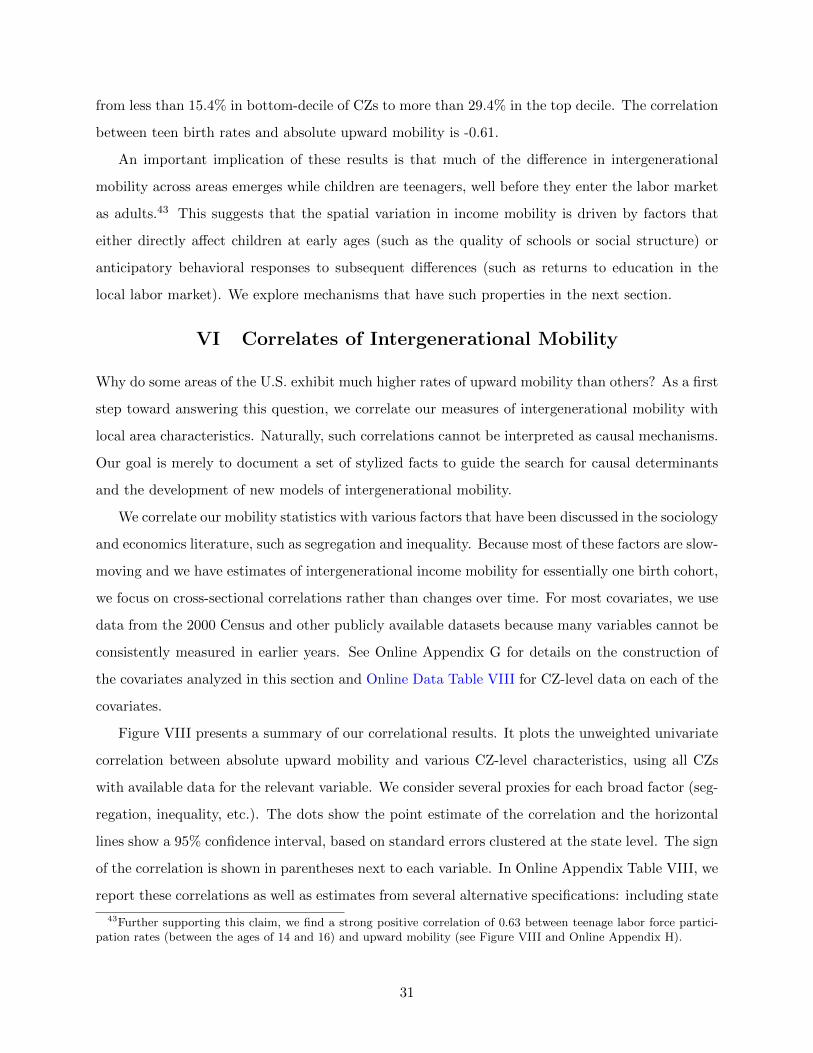
from less than 15.4% in bottom-decile of CZs to more than 29.4% in the top decile. The correlation

between teen birth rates and absolute upward mobility is -0.61.

An important implication of these results is that much of the difference in intergenerational

mobility across areas emerges while children are teenagers, well before they enter the labor market

as adults.43 This suggests that the spatial variation in income mobility is driven by factors that

either directly affect children at early ages (such as the quality of schools or social structure) or

anticipatory behavioral responses to subsequent differences (such as returns to education in the

local labor market). We explore mechanisms that have such properties in the next section.

VI Correlates of Intergenerational Mobility

Why do some areas of the U.S. exhibit much higher rates of upward mobility than others? As a first

step toward answering this question, we correlate our measures of intergenerational mobility with

local area characteristics. Naturally, such correlations cannot be interpreted as causal mechanisms.

Our goal is merely to document a set of stylized facts to guide the search for causal determinants

and the development of new models of intergenerational mobility.

We correlate our mobility statistics with various factors that have been discussed in the sociology

and economics literature, such as segregation and inequality. Because most of these factors are slow-

moving and we have estimates of intergenerational income mobility for essentially one birth cohort,

we focus on cross-sectional correlations rather than changes over time. For most covariates, we use

data from the 2000 Census and other publicly available datasets because many variables cannot be

consistently measured in earlier years. See Online Appendix G for details on the construction of

the covariates analyzed in this section and Online Data Table VIII for CZ-level data on each of the

covariates.

Figure VIII presents a summary of our correlational results. It plots the unweighted univariate

correlation between absolute upward mobility and various CZ-level characteristics, using all CZs

with available data for the relevant variable. We consider several proxies for each broad factor (seg-

regation, inequality, etc.). The dots show the point estimate of the correlation and the horizontal

lines show a 95% confidence interval, based on standard errors clustered at the state level. The sign

of the correlation is shown in parentheses next to each variable. In Online Appendix Table VIII, we

report these correlations as well as estimates from several alternative specifications: including state

43Further supporting this claim, we find a strong positive correlation of 0.63 between teenage labor force partici-pation rates (between the ages of 14 and 16) and upward mobility (see Figure VIII and Online Appendix H).

31

fixed effects, weighting CZs by population, restricting to urban areas, and controlling for differences

in racial demographics and income growth (see Online Appendix H for details). These alternative

specifications generally yield very similar results to the baseline estimates shown in Figure VIII.

Most importantly, the correlations discussed below hold even in specifications with state fixed ef-

fects, showing that the results are not just driven by broad regional differences across the South

vs. other parts of the country. We also show in Online Appendix Table VIII that the factors that

are positively associated with absolute upward mobility are generally positively associated with

relative mobility (i.e., are negatively correlated with rank-rank slopes).

In the remainder of this section, we discuss correlations of mobility with the categories in Figure

VIII that have the strongest relationship with mobility: racial demographics, segregation, income

inequality, school quality, social capital, and family structure. We discuss results for four other

broad categories for which we find weaker correlations – local tax policies, higher education, labor

market conditions, and migration – in Online Appendix H.

VI.A Race

Perhaps the most obvious pattern from the maps in Figure VI is that intergenerational mobility

is lower in areas with larger African-American populations, such as the Southeast. Indeed, the

unweighted correlation between upward mobility and the fraction of black residents in the CZ

(based on the 2000 Census) is -0.580, as shown in the first row of Figure VIII.

This correlation could be driven by two very different channels. One channel is an individual-

level race effect: black children may have lower incomes than white children conditional on parent

income, and hence areas with a larger black population may have lower upward mobility. An

alternative possibility is a place-level race effect: areas with large black populations might have

lower rates of upward mobility for children of all races.

To distinguish between these two channels, we would ideally control for race at the individual

level, essentially asking whether whites have lower rates of upward mobility in areas with a larger

black population. Unfortunately, we do not observe each individual’s race in our data. As an

alternative, we predict race based on the parent’s 5-digit ZIP code (in the year they first claim

their child as a dependent). We use data from the 2000 Census to measure racial shares by

ZIP code. Figure IXa replicates the map of absolute upward mobility (r25,c) by CZ, restricting

the sample to ZIP codes within each CZ in which at least 80% of the residents are non-hispanic

32

whites.44 In this subsample, 91% of individuals are white. The spatial pattern in Figure IXa is

very similar to that in the original map for the full sample in Figure VIa. Most notably, even in

this predominantly white sample, rates of upward mobility remain low in the Southeast and are

much higher in the West. Among the 604 CZs for which we are able to compute upward mobility

measures for predominantly white individuals, the unweighted correlation between upward mobility

for the predominantly white sample and the full sample is 0.91.

In Figure IXb, we generalize this approach to assess how the spatial pattern of upward mobility

changes as we restrict the sample to be increasingly white. To construct this figure, we first

compute upward mobility in each CZ, restricting the sample to individuals living in ZIP codes that

are more than w% white, which we denote by rw25,c. We then regress rw25,c on r25,c, our baseline

estimates of upward mobility based on the full sample, using an unweighted OLS regression with

one observation per CZ with available data. We vary w from 0% to 95% in increments of 5%

and plot the resulting regression coefficients in Figure IXb against the fraction of white individuals

in each of the subsamples. When w = 0, the regression coefficient is 1 by construction because

r25,c = rw=025,c . Since 68% of the U.S. population is white, the first point on the figure is (0.68,

1). The point generated by the w = 80% threshold is (0.91, 0.84), consistent with the map in

Figure IXa. The dotted lines show a 95% confidence interval for the regression coefficients based

on standard errors clustered at the state level.

If the variation in upward mobility across areas were entirely driven by heterogeneity in outcomes

across race at the individual level, the coefficient in Figure IXb would fall to zero as the fraction

white in the sample converged to 1, as illustrated by the dashed line. Intuitively, if all of the spatial

variation in Figure VIa were driven by individual-level differences in race, there would be no spatial

variation left in a purely white sample. The data reject this hypothesis: even in the subsample

with more than 95% white individuals, the regression coefficient remains at 0.89.

The main lesson of this analysis is that both blacks and whites living in areas with large African-

American populations have lower rates of upward income mobility.45 There are many potential

mechanisms for such a correlation, including differences in the institutions and industries that

developed in areas with large African-American populations. We are unable to distinguish between

44We continue to estimate r25,c at the CZ level in this map, but we only include ZIP-5’s within each CZ in which80% or more of the residents are white. To facilitate comparison to Figure VI, we color the entire CZ based on thisstatistic, including ZIP-5’s whose own white share is below 80%. CZs that have fewer than 250 children who grewup in ZIP codes where more than 80% of the residents are white are omitted (and shown with cross-hatch shading).

45To be clear, this result does not imply that race does not matter for children’s outcomes at the individual level,as shown e.g. by Mazumder (2011). Our finding is simply that there is spatial heterogeneity in upward mobility evenconditional on race.

33

these mechanisms in our data; instead, we next turn to one such mechanism that has received the

greatest attention in prior work: segregation. The U.S. has a historical legacy of greater segregation

in areas with more blacks. Such segregation could potentially affect both low-income whites and

blacks, as racial segregation is often associated with income segregation.

VI.B Segregation

Prior work has argued that segregation has harmful effects on disadvantaged individuals through

various channels: reducing exposure to successful peers and role models, decreasing funding for local

public goods such as schools, or hampering access to nearby jobs (Wilson 1987, Massey and Denton

1993, Cutler and Glaeser 1997). In this subsection, we evaluate these hypotheses by exploring the

correlation between intergenerational mobility and various measures of segregation (shown in the

second panel of Figure VIII and Online Appendix Table VIII).

We begin by measuring racial segregation using a Theil (1972) index, constructed using data

from the 2000 Census as in Iceland (2004). Let φr denote the fraction of individuals of race r in a

given CZ, with four racial groups: whites, blacks, hispanics, and others. We measure the level of

racial diversity in the CZ by an entropy index: E =∑φr log2

1φr

, with φrlog21φr

= 0 when φr = 0.

Letting j = 1, ..., N index census tracts in the CZ, we analogously measure racial diversity within

each tract as Ej =∑φrj log2

1φrj

where φrj denotes the fraction of individuals of race r in tract j.

We define the degree of racial segregation in the CZ as

H =∑j

[popj

poptotal

E − EjE

] (4)

where popj denotes the total population of tract j and poptotal denotes the total population of

the CZ. Intuitively, H measures the extent to which the racial distribution in each Census tract

deviates from the overall racial distribution in the CZ. The segregation index H is maximized at

H = 1 when there is no racial heterogeneity within census tracts, in which case Ej = 0 in all tracts.

It is minimized at H(p) = 0 when all tracts have racial composition identical to the CZ as a whole,

so that Ej = E.

Column 1 of Table IV reports the coefficient estimate from an unweighted OLS regression of

absolute upward mobility r25,c on the racial segregation index, with one observation per CZ. In this

and all subsequent regressions, we standardize the dependent variable and all independent variables

to have mean 0 and standard deviation 1 within the estimation sample. Hence, the coefficients in the

univariate regressions can be interpreted as correlation coefficients. Standard errors are clustered

34

by state to account for spatial correlation across CZs.

More racially segregated areas have less upward mobility. The unweighted correlation between

upward mobility and the racial segregation index in Column 1 is -0.361.46 Column 2 shows that

the correlation remains at -0.360 in urban areas, i.e. CZs that overlap with metropolitan statistical

areas (MSAs).

Next, we turn to the relationship between income segregation and upward mobility. Following

Reardon and Firebaugh (2002) and Reardon (2011), we begin by measuring the degree to which

individuals below the pth percentile of the local household income distribution are segregated from

individuals above the pth percentile in each CZ using a two-group Theil index H(p). Here, entropy

in a given area is E(p) = p log21p + (1− p) log2

11−p and the index H(p) is defined using the formula

in (4). Building on this measure, Reardon (2011) defines the overall level of income segregation in

a given CZ as

income segregation = 2log(2)´pE(p)H(p)dp. (5)

This measure is simply a weighted average of segregation at each percentile p, with greater weight

placed on percentiles in the middle of the income distribution, where entropy E(p) is maximized.

We implement (5) using data from the 2000 Census, which reports income binned in 16 categories.

Following Reardon (2011, Appendix 3), we measure H(p) at each of these cutoffs and take a

weighted sum of these values to calculate income segregation.

In Column 3 of Table IV, we regress absolute upward mobility on the income segregation index;

see Online Appendix Figure Xb for the corresponding non-parametric binned scatter plot. The

correlation between income segregation and upward mobility is -0.393, consistent with the findings

of Graham and Sharkey (2013) using survey data. Interestingly, areas with a larger black population

exhibit greater income segregation: the correlation between the fraction of black individuals in a

CZ and the income segregation index is 0.264 (s.e. 0.082). Hence, the negative relationship between

income segregation and upward mobility could partly explain why low-income white children fare

more poorly in areas with large African-American populations.

In Column 4, we decompose the effects of segregation in different parts of the income distribu-

tion. Following Reardon and Bischoff (2011), we define the “segregation of poverty” as H(p = 25),

i.e. the extent to which individuals in the bottom quartile are segregated from those above the 25th

percentile. We analogously define the segregation of affluence as H(p = 75). Column 4 regresses

46Online Appendix Figure Xa presents a non-parametric binned scatter plot corresponding to this regression; seeOnline Appendix H for details on the construction of this figure.

35

upward mobility on both segregation of poverty and affluence. Segregation of poverty has a strong

negative association with upward mobility, whereas segregation of affluence does not. Column 5

shows that the same pattern holds when restricting the sample to urban areas. These results sug-

gest that the isolation of low-income families (rather than the isolation of the rich) may be most

detrimental for low income children’s prospects of moving up in the income distribution.

Another mechanism by which segregation may diminish upward mobility is through spatial

mismatch in access to jobs (Kain 1968, Kasarda 1989, Wilson 1996). We explore this mechanism in

Column 6 by correlating upward mobility with the fraction of individuals who commute less than

15 minutes to work in the CZ, based on data from the 2000 Census. Areas with less sprawl (shorter

commutes) have significantly higher rates of upward mobility; the correlation between commute

times and upward mobility is 0.605. Column 7 shows that commute times remain a significant

predictor of upward mobility in a multivariable regression but income segregation does not.

These results are consistent with the view that the negative impacts of segregation may operate

by making it more difficult to reach jobs or other resources that facilitate upward mobility. But any

such spatial mismatch explanation must explain why the gradients emerge before children enter

the labor market, as shown in Section V.E. A lack of access to nearby jobs cannot directly explain

why children from low-income families are also more likely to have teenage births and less likely to

attend college in cities with low levels of upward mobility. However, spatial mismatch could produce

such patterns if it changes children’s behavior because they have fewer successful role models or

reduces their perceived returns to education.

VI.C Income Levels and Inequality

In this subsection, we explore the correlation between properties of the local income distribution –

mean income levels and inequality – and intergenerational mobility.

Mean Income Levels. The third section of Figure VIII shows that the mean level of household

income in a CZ (as measured in the 2000 Census) is essentially uncorrelated with upward mobility

(see Online Appendix Figure XIa for the corresponding non-parametric binned scatter plot). Chil-

dren in low-income families who grow up in the highest-income CZs (with mean incomes of $47,600

per year) reach almost exactly the same percentile of the national income distribution on average

as those who grow up in the lowest-income areas (with mean incomes of $21,900).

Income Inequality. Prior work has documented a negative correlation between income inequal-

ity and intergenerational mobility across countries (e.g., Corak 2013). This “Great Gatsby” curve

36

(Krueger 2012) has attracted attention because it suggests that greater inequality within a gener-

ation could reduce social mobility. We explore whether there is an analogous relationship across

areas within the U.S. by correlating upward mobility with the Gini coefficient of parent income

within each CZ. We compute the Gini coefficient for parents in our core sample within each CZ as

Gini = 2XcCov(Xic, Pic), where Xc is the mean family income (from 1996-2000) of parents in CZ c

and Cov(Xic, Pic) is the covariance between the income level (Xic) and the percentile rank (Pic) of

parents in CZ c. The correlation between the Gini coefficient and upward mobility is -0.578 (see

also Online Appendix Figure XIb).

An alternative measure of inequality is the portion of income within a CZ that accrues to the

richest households, e.g. those in the top 1%. This measure is of particular interest because the rise

in inequality in the U.S. over the past three decades was driven primarily by an increase in top

income shares (Piketty and Saez 2003). We calculate top 1% income shares using the distribution

of parent family income within each CZ. The correlation between upward mobility and the top 1%

income share is only -0.190 (see also Online Appendix Figure XIc), much weaker than that with

the Gini coefficient.

We investigate why the Gini coefficient and top 1% share produce different results in Table V,

which is constructed in the same way as Table IV. Column 1 replicates the regression corresponding

to the raw correlation between the Gini coefficient and upward mobility as a reference. We de-

compose the Gini coefficient into inequality coming from the upper tail and the rest of the income

distribution by defining the bottom 99% Gini as the Gini coefficient minus the top 1% income

share. The bottom 99% Gini can be interpreted as the deviation of the Lorenz curve from perfect

equality amongst households in the bottom 99%. Column 2 of Table V shows that a 1 SD increase

in the bottom 99% Gini is associated with a 0.634 SD reduction in upward mobility. In contrast, a

1 SD increase in the top 1% share is associated with only a 0.123 SD reduction in upward mobility.

Column 3 shows that in urban areas (CZs that overlap with MSAs), the pattern is even more stark:

upper tail inequality is uncorrelated with upward mobility, whereas the Gini coefficient within the

bottom 99% remains very highly strongly correlated with upward mobility.

Another measure of inequality within the bottom 99% is the size of the middle class in the CZ,

which we define as the fraction of parents in the CZ who have family incomes between the 25th

and 75th percentiles of the national parent income distribution. Column 4 of Table V shows that

upward mobility is strongly positively correlated with the size of the middle class.

Finally, Column 5 of Table V replicates Column 2 using relative mobility βc as the dependent

37

variable. The bottom 99% Gini coefficient is strongly positively associated with this measure. That

is, greater inequality in the bottom 99% is negatively related to relative mobility.47 But once again,

the top 1% share is uncorrelated with relative mobility.

Comparison to Cross-Country Evidence. Next, we explore whether the size of the middle class

is more strongly correlated with intergenerational mobility than upper tail inequality in the cross-

country data as well. In Column 6 of Table V, we replicate Corak’s (2013, Figure 1) result that

there is a strong positive correlation between the Gini coefficient (as measured in survey data on

income in 1985) and the intergenerational elasticity (IGE) using data from 13 developed countries

compiled by Corak (2013).48 In Column 7, we include the top 1% income share in each country,

based on statistics from the World Top Incomes Database. As in the within-U.S. analysis, there is

little correlation between the top 1% income share and intergenerational mobility across countries.

Column 8 shows that results are similar if one uses inequality measures from 2005 instead of 1985.

We conclude that there is a robust negative correlation between inequality within the current

generation of adults and mobility across generations. However, intergenerational mobility is pri-

marily correlated with inequality among the bottom 99% and not the extreme upper tail inequality

of the form that has increased dramatically in recent decades. Interestingly, this pattern parallels

the results we obtained for segregation above: segregation of affluence is not significantly correlated

with intergenerational mobility, while segregation of poverty is negatively associated with mobility.

VI.D School Quality

In the fourth panel of Figure VIII, we study the correlation between mobility and various proxies

for school quality. We first consider two proxies for inputs into school quality: mean public school

expenditures per student and mean class sizes based on data from the National Center for Education

Statistics (NCES) for the 1996-97 school year. We find a positive correlation between public school

expenditures and upward mobility, but the correlation is not as strong or robust as with measures

of inequality or segregation. There is a strong negative correlation between class size and upward

mobility (Columns 1 and 2 of Online Appendix Table VIII) when pooling all CZs. However, there

is no correlation between upward mobility and class size in more urban areas (Columns 3 and 4).

One shortcoming of input-based measures of school quality is that they may capture relatively

47Because parent and child ranks are measured in the national income distribution, there is no mechanical rela-tionship between the level of inequality within the CZs income distribution and the rank-rank slope.

48We obtain estimates of the Gini coefficient by country from the OECD Income Distribution Database. Weinterpret these estimates as applying to the bottom 99% because surveys typically do not capture the thickness ofthe top tail due to top-coding.

38

little of the variation in school quality (Hanushek 2003). To address this problem, we construct

output-based proxies for school quality based on test scores and dropout rates adjusted for differ-

ences in parent income. We obtain data on mean grade 3-8 math and English test scores by CZ from

the Global Report Card. The Global Report Card converts school-district-level scores on statewide

tests to a single national scale by benchmarking statewide test scores to scores on the National

Assessment of Educational Progress (NAEP) tests. We obtain data on high school dropout rates

from the NCES for the 2000-01 school year, restricting the sample to CZs in which at least 75% of

school districts have non-missing data. We regress test scores on mean parent family income (from

1996-2000) in the core sample and compute residuals to obtain an income-adjusted measure of test

score gains. We construct an income-adjusted measure of dropout rates analogously.

The income-adjusted test score and dropout rates are very highly correlated with upward mobil-

ity across all specifications, as shown in the fourth panel of Figure VIII. In the baseline specification,

the magnitude of the correlation between both measures and upward mobility is nearly 0.6. These

results are consistent with the hypothesis that the quality of schools – as judged by outputs rather

than inputs – plays a role in upward mobility. At a minimum, they strengthen the view that

much of the difference in intergenerational income mobility across areas emerges while children are

relatively young.

VI.E Social Capital

Several studies have emphasized the importance of social capital – the strength of social networks

and engagement in community organizations in local areas – for social and economic outcomes

(e.g., Coleman 1988, Borjas 1992, Putnam 1995). We explore the relationship between mobility

and measures of social capital used in prior work in the fifth panel of Figure VIII.

Our primary proxy for social capital is the social capital index constructed by Rupasingha and

Goetz (2008), which we aggregate to the CZ level using population-weighted means. This index is

comprised of voter turnout rates, the fraction of people who return their census forms, and various

measures of participation in community organizations. The correlation between upward mobility

and social capital is 0.641 in our baseline specification, an estimate that is quite robust across

alternative specifications. Interestingly, one of the original measures proposed by Putnam (1995) –

the number of bowling alleys in an area – has an unweighted correlation of 0.562 with our measures

of absolute upward mobility.

We also consider two other proxies for social capital: the fraction of religious individuals (based

39

on data from the Association of Religion Data Archives) and the rate of violent crime (using data

from the Uniform Crime Report). Religiosity is very strongly positively correlated with upward

mobility, while crime rates are negatively correlated with mobility.

VI.F Family Structure

Many have argued that family stability plays a key role in children’s outcomes (see e.g., Becker

1991, Murray 1984, Murray 2012). To evaluate this hypothesis, we use three measures of family

structure in the CZ based on data from the 2000 Census: (1) the fraction of children living in

single-parent households, (2) the fraction of adults who are divorced, and (3) the fraction of adults

who are married. All three of these measures are very highly correlated with upward mobility, as

shown in the sixth panel of Figure VIII.

The fraction of children living in single-parent households is the single strongest correlate of

upward income mobility among all the variables we explored, with a raw unweighted correlation of

-0.76 (see Online Appendix Figure XIIa for the corresponding non-parametric binned scatter plot).

One natural explanation for this spatial correlation is an individual-level effect: children raised by a

single parent may have worse outcomes than those raised by two parents (e.g., Thomas and Sawhill

2002, Lamb 2004). To test whether this individual-level effect drives the spatial correlation, we

calculate upward mobility in each CZ based only on the subsample of children whose own parents

are married. The correlation between upward mobility and the fraction of single parents in their

CZ remains at -0.66 even in this subgroup (Online Appendix Figure XIIb). Hence, family structure

correlates with upward mobility not just at the individual level but also at the community level,

perhaps because the stability of the social environment affects children’s outcomes more broadly.

The association between mobility and family structure at the community level echoes our findings

in Section VI.A on the community-level effects of racial shares.

VI.G Comparison of Alternative Explanations

In Table VI, we assess which of the five factors identified above – segregation, inequality, school

quality, social capital, and family structure – are the strongest predictors of upward mobility in

multivariable regressions that control for race and other covariates. Based on the analysis above, we

first identify the proxy that has the strongest and most robust univariate correlation with upward

mobility in each category: the fraction of working individuals who commute less than 15 minutes to

work (segregation), the bottom 99% Gini coefficient (inequality), high school dropout rates adjusted

40

for income differences (school quality), the social capital index, and the fraction of children with

single parents (family structure).49 As in preceding regression specifications, we normalize all the

dependent and independent variables to have a standard deviation of 1 in the estimation sample

for each regression in Table VI.50

We begin in Column 1 with an unweighted OLS regression of absolute upward mobility r25,c

on the five factors, pooling all CZs. All of the factors except the Gini coefficient are significant

predictors of the variation in absolute upward mobility in this specification. Together, the five

factors explain 76% of the variance in upward mobility across areas. Column 2 shows that the

coefficients remain similar when state fixed effects are included. Column 3 shows that the estimates

are roughly similar when restricting the sample to urban areas (CZs that intersect MSAs). Across

all the specifications, the strongest and most robust predictor is the fraction of children with single

parents.

In Column 4, we use relative mobility βc as the dependent variable instead of absolute upward

mobility. The fraction of single-parents and commute times are strong predictors of differences in

relative mobility across areas, but the other factors are not statistically significant. To understand

why this is the case, in Column 5 we replicate Column 4 but exclude the fraction of children with

single parents. In this specification, all four of the remaining factors – including the Gini coefficient

– are strong predictors of the variation in relative mobility across CZs. Column 6 replicates the

specification in Column 5 using absolute upward mobility as the dependent variable. Once again, all

four factors are strong predictors of upward mobility when the fraction of single parents is excluded.

These results suggest that the fraction of single parents may capture some of the variation in the

other factors, most notably the level of income inequality.

In the last two columns of Table VI, we explore the role of racial demographics vs. the other

explanatory factors. Column 7 shows that when we regress absolute upward mobility on both

the fraction of single-parent families in the CZ and the share of black residents, black shares are

no longer significantly correlated with upward mobility. Column 8 shows that the correlation of

upward mobility with black shares is slightly positive and statistically significant when we include

controls for all five explanatory factors. These results support the view that the strong correlation

49We obtain similar results if we combine the various proxies into a single index for each factor using weights froman OLS regression of absolute upward mobility on the proxies within each category.

50We code the high school dropout rate as 0 for 126 CZs in which dropout rate data are missing for more than25% of the districts in the CZ and include an indicator for having a missing high school dropout rate. We do thesame for 16 CZs that have missing data on social capital. We normalize these variables to have mean 0 and standarddeviation 1 among the CZs with non-missing data.

41

of upward mobility with race operates through channels beyond the direct effect of race on mobility.

Overall, the results in Table VI indicate that the differences in upward mobility across areas

are better explained by a combination of the factors identified above rather than any single factor.

However, the regression coefficients should be interpreted with caution for two reasons. First, the

regression may place greater weight on factors that are measured with less error rather than those

that are truly the strongest determinants of mobility. Second, all of the independent variables are

endogenously determined. These limitations make it difficult to identify which of the factors is the

most important determinant of upward mobility.

VII Conclusion

This paper has used population data to present a new portrait of intergenerational income mobility

in the United States. Intergenerational mobility varies substantially across areas. For example, the

probability that a child reaches the top quintile of the national income distribution starting from

a family in the bottom quintile is 4.4% in Charlotte but 12.9% in San Jose. The spatial variation

in intergenerational mobility is strongly correlated with five factors: (1) residential segregation, (2)

income inequality, (3) school quality, (4) social capital, and (5) family structure.

In this paper, we have presented a cross-sectional snapshot of intergenerational mobility for

a single set of birth cohorts. In a companion paper (Chetty et al. 2014), we study trends in

mobility over time. We find that the level of intergenerational mobility (national rank-rank slope)

has remained stable for the 1971-1993 birth cohorts in the U.S., especially in comparison to the

degree of variation across areas. A natural question given the results of the two papers is whether

the cross-sectional correlations documented here are consistent with the time trends in mobility.

To answer this question, we predict the trend in the rank-rank slope implied by changes in the

five key correlates over time (see Online Appendix I and Appendix Figure XIII). The predicted

changes are quite small because the factors move in opposing directions. For example, the increase

in inequality and single parenthood rates in recent decades predict a small decline in mobility in

recent decades. In contrast, the decline in racial segregation and high school dropout rates predict

an increase in mobility of similar magnitude. Overall, the cross-sectional correlations documented

here are consistent with the lack of a substantial time trend in mobility in recent decades.

The main lesson of our analysis is that intergenerational mobility is a local problem, one that

could potentially be tackled using place-based policies (Kline and Moretti 2014). Going forward,

a key question is why some areas of the U.S. generate higher rates of mobility than others. We

42

hope that future research will be able to shed light on this question by using the mobility statistics

constructed here (available online at the county by birth cohort level) to study the impacts of local

policy changes.

43

ONLINE APPENDICES

A. Data Construction

Core and Extended Samples. We begin with the universe of individuals in the Death Master(also known as the Data Master-1) file produced by the Social Security Administration. This fileincludes information on year of birth and gender for all persons in the United States with a SocialSecurity Number or Individual Taxpayer Identification Number. We restrict this sample to allindividuals who are current US citizens as of March 2013. The Data Master-1 file does not containhistorical citizenship status, and thus we can only restrict to a sample who are currently US citizensas of the time at which we access the data. We further restrict to individuals who are alive throughthe end of 2012. The resulting dataset contains 47.8 million children across all cohorts 1980-1991(Appendix Table I). We measure parent and child income, location, college attendance, and allother variables using data from the IRS Databank, a balanced panel covering all individuals in theUnited States who appear on any tax form between 1996-2012.

For each child, we define the parent(s) as the first person(s) who claim the child as a dependenton a 1040 tax form. If parents are married but filing separately, we assign the child both parents.To eliminate dependent claiming by siblings or grandparents, in the case of a potential match tomarried parents or single mothers, we require the mother to be age 15-40 at the birth of the child.51

In the case of a match to a single father, we require the father to be age 15-40 at the birth of thechild. If no such eligible match occurs in 1996, the first year of our data, we search subsequentyears (through 2011) until a valid match is found.

Once we match a child to parent(s), we hold this definition of parents fixed regardless of sub-sequent dependent claims or changes in marital status. For example, a child matched to marriedparents in 1996 who divorce in 1997 will always be matched to the two original parents. Conversely,a child matched to a single parent in 1996 that marries in 1997 will be considered matched to asingle parent, though spouse income will be included in our definition of parent income because wemeasure parent income at the family level in our baseline analysis.

To reduce the effects of outliers and measurement error in the upper tail of the income dis-tribution, we use data from the IRS Statistics of Income (SOI) manually perfected cross-sectionalfiles spanning 1996-2011 (see below for details on these files). If an individual’s adjusted grossincome exceeds $10 million, we look for the individual in the SOI sample; if present, we use theSOI measure of adjusted gross income and wage income as reported on a F1040 return. If not, wereplace the adjusted gross income with the total wages reported on the filed F1040 contained in thedatabank. Because the IRS Databank includes tax year 2012 whereas the SOI sample does not, wetop code income at $100 million for all individuals in 2012. These adjustments in the upper tailaffect 0.017% of parents in our core sample (or, equivalently, 1.7% of parents in the top 1% of theincome distribution).

For most of our analysis, we measure parent income at the household level. For certain robust-ness checks, we measure individual parent income as follows. For married parents, we define eachparent’s individual earnings as the sum of wage earnings from form W-2, unemployment benefitsfrom form 1099-G, and Social Security and Disability benefits from form SSA-1099 for that individ-ual. Individual earnings excludes capital and other non-labor income. To incorporate these sources

51Children can be claimed as a dependent only if they are aged less than 19 at the end of the year (less than 24 ifenrolled as a student) or are disabled. A dependent child is a biological child, step child, adopted child, foster child,brother or sister, or a descendant of one of these (for example, a grandchild or nephew). Children must be claimed bytheir custodial parent, i.e. the parent with whom they live for over half the year. Furthermore, the custodial parentmust provide more than 50% of the support to the child. Hence, working children who support themselves for morethan 50% cannot be claimed as dependents. See IRS Publication 501 for further details.

44

of income, we add half of family non-labor income – defined as total family income minus totalfamily earnings reported on form 1040 – to each parent’s individual earnings. We divide non-laborearnings equally between spouses because we cannot identify which spouse earns non-labor incomefrom the 1040 tax return. For single parents, individual income is the same as family income.

Statistics of Income Sample. Starting in 1987, the IRS Statistics of Income cross sections –which are stratified random samples of tax returns – contain dependent information, allowing usto link children to parents. We use the 1987-2011 SOI cross-sections to construct a sample ofchildren born in the 1971-1991 birth cohorts and correct for errors in the upper tail of the incomedistribution as described above. For each SOI cross-section from 1987 to 2007, we first identifyall dependent children between the ages of 12 and 16 who are alive at age 30. We then pool allthe SOI cross-sections that give us information for a given birth cohort. For example, the 1971cohort is represented by children claimed at age 16 in 1987, while the 1991 cohort is comprised bychildren claimed at ages 12-16 in 2003-2007. Using the sampling weights for the SOI cross-sections(see Internal Revenue Service (2013) for details), each cohort-level dataset is representative of thepopulation of children claimed on tax returns between the ages of 12 and 16 in that birth cohort.

Unlike in the population-based samples, we do not limit the SOI sample to children who arecurrently citizens because citizenship data are not fully populated for birth cohorts prior to 1980 andbecause we begin from a sample of children claimed by parents rather than the universe of childrenwho currently appear in the population data (which includes later immigrants). In the years wherethe SOI and population-based samples overlap, we obtain very similar estimates in both samples.The citizenship restriction has a minor impact because the vast majority of children claimed asdependents between the ages of 12-16 are U.S. citizens as adults. We also do not impose any agerestrictions on the parents in the SOI sample. In the population-based sample, some children areclaimed by different adults across years and the age restriction is useful to discriminate betweenthese potential parents. In the SOI sample, each child can only be linked to the parents who claimhim in the cross-section file, so the age restriction would not play such a role. In practice, thisrestriction has little impact, as the age distribution of parents in the SOI sample is very similar tothat in the core sample using the population data.

Children whose parents are sampled in multiple SOI cross-sections appear multiple times in theSOI sample. There are 228,295 unique children in the SOI sample and 523,700 total observations.The SOI sample grows from 4,383 unique children in 1971 to 21,231 unique children in 1991 becausewe have more cross-sections to link parents to children in more recent cohorts and because the sizeof the SOI cross-sections has increased over time (Appendix Table II). To be consistent with thecore sample definition of parent income, we define parent income as the 5-year average of parentfamily income from 1996-2000 in the IRS Databank.

We provide additional information on the SOI sample in Chetty et al. (2014). Using samplingweights, we show that the SOI sample represents roughly 85% of children in each birth cohort (basedon vital statistics counts) from 1971-1979, the cohorts we use to obtain estimates of intergenerationalmobility after age 32 in Figure IIIa. We also show that summary statistics for the SOI sample arevery similar to the core sample for the 1980-82 birth cohorts reported in Appendix Table III of thispaper. Note that Chetty et al. (2014) compute parent income using the income of the parents inthe single year of the parent-child match there, whereas we compute parent income as the five-yearaverage over 1996-2000 here for consistency with results from the population data. Because werestrict to parents with positive income, this leads to a small difference in the SOI sample usedacross the two papers. For example, we have 4,383 children in the 1971 cohort, compared with4,331 children in the sample used by Chetty et al. (2014).

Assignment of Children to Commuting Zones. Children are assigned ZIP codes of residencebased on their parents’ ZIP code on the form 1040 in which the parent is matched to the child. In

45

the few cases where a parent files a F1040 claiming the child but does not report a valid ZIP code,we search information returns (such as W-2 and 1099-G forms) for a valid ZIP code in that year.

We map these ZIP codes to counties based on the 1999 Census crosswalk between ZIP codesand counties. We then aggregate counties into Commuting Zones using David Dorn’s county-to-CZcrosswalk (download file E6). The counties in the U.S. Census Bureau crosswalk and in Dorn’scrosswalk are not identical because they correspond to county definitions at different points intime; in particular the U.S. Census Bureau crosswalk includes changes between 1990 and 1999. Wemake manual adjustments for changes that affected 200 or more people. Using this procedure, weidentify the CZ of 38,839 ZIP codes. To track individuals residing in ZIP codes that have beencreated since 1999, we add an additional 477 ZIP codes not valid in 1999 but appearing in the moreup-to-date 2011 HUD-USPS crosswalk. For example, in 2007, Manhattan’s ZIP code 10021 wassplit into three separate ZIP codes, resulting in the creation of new ZIP codes 10065 and 10075.

Of 9,864,965 children with non-missing ZIP codes in our core sample, 9,778,071 were assigned achildhood CZ using ZIP codes that existed in 1999; an additional 2,718 were assigned a CZ basedon a ZIP code that existed in 2011 but not in 1999. For simplicity, we use the same crosswalk for allyears of matching ZIP codes to CZs. We have verified that using year-specific crosswalks from ZIPcodes to counties has a negligible effect on CZ assignments. All of the crosswalks we constructedare available on our project website.

Some of our specifications require tracking children’s locations into adulthood using the ZIPcode where they live as adults when we measure their income (e.g., for cost-of-living adjustments).We define a child’s adult location using the latest non-missing ZIP code. We first search for a ZIPcode in their 1040 form in 2012, followed by their information returns in 2012. We then repeatthis procedure for 2011 if we do not find a zipcode in 2012. This yields 9,834,975 non-missing childZIP codes in adulthood. Of these, we match 9,537,283 to a CZ from a ZIP code using the 1999crosswalk (i.e. this ZIP code was in use in 1999) and an additional 198,317 using the later crosswalkbecause the ZIP code was created after 1999.

Construction of ZIP-Level Racial Shares. To construct Figure IXa and IXb, which conditionon racial shares at the ZIP level, we need data on racial shares by ZIP code. The 2000 Censusincludes summary tables by ZIP code tabulation areas (ZCTAs) instead of ZIP code. ZCTAs area U.S. Census Bureau geographical unit that in most cases correspond closely to ZIP codes, butsometimes do not. We use a ZCTA to ZIP Crosswalk from the John Snow Institute to assign eachZIP code a racial share based on Census 2000 ZCTA-level data from table P008.

CZ-Level Price Index. To measure real incomes, we first construct a CZ-level ACCRA priceindex using the 2010 ACCRA composite cost of living index (table 728) for “urbanized areas”in 2010, which we crosswalk to CZs as follows. First, we use the 2012Q1-2013Q1 correspondence(downloaded on 11/21/2013) to assign 298 out of the 325 urbanized areas to MSAs. Each county inan MSA was assigned the same value of the index. We then merge counties to CZs and calculate anunweighted mean of the index among non-missing values within the CZ. Some CZs had no countieswithin an MSA and were therefore assigned a missing value of the ACCRA index.

To construct a price index that covers all CZs, we regress the CZ-level ACCRA index on aquadratic in log population density (from the 2000 Census), a quadratic in log median housingvalues, the latitude and longitude of the CZ centroid, and state fixed effects. Housing values arethe population-weighted mean of tract median housing values for owner-occupied units in the 1990Census short form. Latitude and longitude are the mean latitude and longitude across countieswithin each CZ, obtained from the Census 2000 Gazetteer county-level data. The predicted valuesfrom this regression constitute our final price index that covers all CZs.

B. Comparison to Survey Datasets

46

In Appendix Table IV, we compare selected moments of income distributions and other variablesin the tax data to data from two nationally representative surveys that have been used in priorwork on the income distribution: the 2011-12 CPS and the 2011-12 ACS. We restrict the ACS andCPS samples to citizens in the same birth cohorts as our core sample (1980-82). To the extentpossible, we define all income variables to match the concepts in the tax data.

To assess whether our method of linking children to parents based on dependent claiming createsselection bias, we compute statistics in the tax data both on the full sample of all children in the1980-82 birth cohorts who are current U.S. citizens and the core sample of children linked to parents.Because most children are linked to parents, the differences between these two samples are small,though children who lack valid parent matches have slightly lower earnings on average.

Overall, the tax data are very similar to the CPS and ACS. The sum of the sampling weightsin our survey-based samples provide estimates of the size of the target population being sampled.This population is very similar in the tax data and the two surveys. The mean and median earningslevels are very similar, as are the fractions with non-zero income. Perhaps more surprisingly, theinterquartile range (P75-P25) of earnings is also similar across the three data sources. If surveydata were reported with classical measurement error, we would expect the interquartile range to belarger in survey sources. However, survey reports of income exhibit “mean reverting” measurementerror which has the effect of reducing variability (Bound and Krueger 1991, Bound, Brown andMathiowetz 2001). Moreover, survey non-response tends to follow a U-shaped pattern (Kline andSantos 2013), with very high and low earning individuals being least likely to provide earningsresponses, which can further reduce variability. The quantiles of family income also line up wellacross the three data sources, with the tax-based moments strongly resembling those from the ACS,perhaps because the ACS has a higher response rate for earnings than the CPS.

C. Comparison to Mitnik et al. (2014)

Mitnik et al. (2014) propose a new measure of the intergenerational elasticity that is morerobust to the treatment of small incomes. In this appendix, we compare the traditional definitionof the IGE (Solon 1999, Black and Devereux 2011) to the new measure proposed by Mitnik et al.We first show that the traditional IGE can be interpreted as the average elasticity of child incomewith respect to parent income in a model with heterogeneous elasticities, while Mitnik et al.’s newmeasure is a dollar-weighted (i.e., child-income-weighted) average of the same elasticity. We thencompare estimates of the dollar-weighted IGE to estimates of the traditional IGE in our data andto the estimates of Mitnik et al.

Setup. Let Yi denote the level of child income and Xi denote the level of parent income. LetFY |X=x (y) denote the conditional distribution of Y given X, which we assume is differentiable withrespect to x at all (y, x) > 0. Define the conditional quantile function (CQF) as the inverse of theCDF:

q(x, τ) = F−1Y |X=x (τ)

for τ ∈ [0, 1].52 The CQF gives the quantiles of the conditional distribution of Yi given Xi; forexample, q (x, .5) is the median of Yi when Xi = x.

We can use the CQF to represent Yi as:

Yi = q (Xi, Ui) ,

where Ui|Xi ∼ Uniform (0, 1). Hence, the conditional mean of child income given parent income

52At mass points, we define q(x, τ) ≡ inf{y : FY |X=x (y) ≥ τ

}.

47

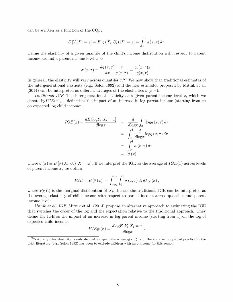
can be written as a function of the CQF:

E [Yi|Xi = x] = E [q (Xi, Ui) |Xi = x] =

ˆ 1

0q (x, τ) dτ.

Define the elasticity of a given quantile of the child’s income distribution with respect to parentincome around a parent income level x as

σ (x, τ) ≡ dq (x, τ)

dx

x

q (x, τ)=qx(x, τ)x

q(x, τ).

In general, the elasticity will vary across quantiles τ .53 We now show that traditional estimates ofthe intergenerational elasticity (e.g., Solon 1992) and the new estimator proposed by Mitnik et al.(2014) can be interpreted as different averages of the elasticities σ (x, τ).

Traditional IGE. The intergenerational elasticity at a given parent income level x, which wedenote byIGE(x), is defined as the impact of an increase in log parent income (starting from x)on expected log child income:

IGE(x) =dE [logYi|Xi = x]

dlogx=

d

dlogx

ˆ 1

0logq (x, τ) dτ

=

ˆ 1

0

d

dlogxlogq (x, τ) dτ

=

ˆ 1

0σ (x, τ) dτ

= σ (x)

where σ (x) ≡ E [σ (Xi, Ui) |Xi = x]. If we interpret the IGE as the average of IGE(x) across levelsof parent income x, we obtain

IGE = E [σ (x)] =

ˆ ∞−∞

ˆ 1

0σ (x, τ) dτdFX (x) ,

where FX (.) is the marginal distribution of Xi. Hence, the traditional IGE can be interpreted asthe average elasticity of child income with respect to parent income across quantiles and parentincome levels.

Mitnik et al. IGE. Mitnik et al. (2014) propose an alternative approach to estimating the IGEthat switches the order of the log and the expectation relative to the traditional approach. Theydefine the IGE as the impact of an increase in log parent income (starting from x) on the log ofexpected child income:

IGEW (x) ≡ dlogE [Yi|Xi = x]

dlogx.

53Naturally, this elasticity is only defined for quantiles where q(x, τ) > 0; the standard empirical practice in theprior literature (e.g., Solon 1992) has been to exclude children with zero income for this reason.

48

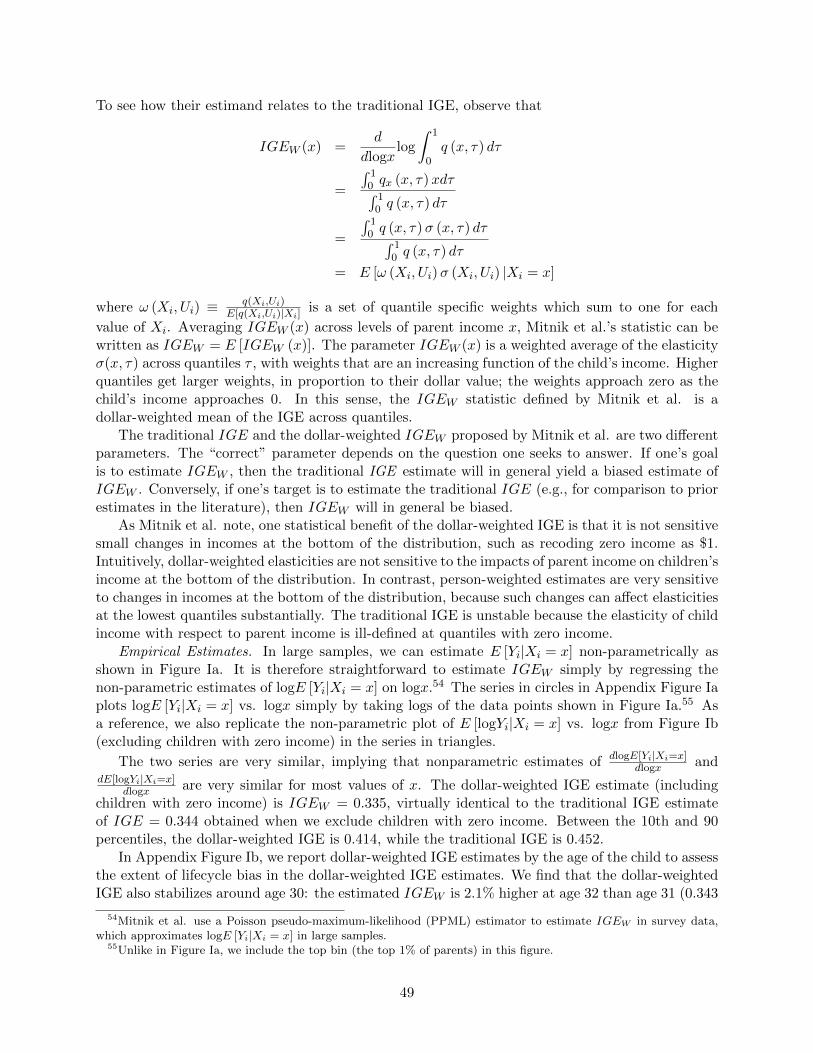
To see how their estimand relates to the traditional IGE, observe that

IGEW (x) =d

dlogxlog

ˆ 1

0q (x, τ) dτ

=

´ 10 qx (x, τ)xdτ´ 1

0 q (x, τ) dτ

=

´ 10 q (x, τ)σ (x, τ) dτ´ 1

0 q (x, τ) dτ

= E [ω (Xi, Ui)σ (Xi, Ui) |Xi = x]

where ω (Xi, Ui) ≡ q(Xi,Ui)E[q(Xi,Ui)|Xi]

is a set of quantile specific weights which sum to one for each

value of Xi. Averaging IGEW (x) across levels of parent income x, Mitnik et al.’s statistic can bewritten as IGEW = E [IGEW (x)]. The parameter IGEW (x) is a weighted average of the elasticityσ(x, τ) across quantiles τ , with weights that are an increasing function of the child’s income. Higherquantiles get larger weights, in proportion to their dollar value; the weights approach zero as thechild’s income approaches 0. In this sense, the IGEW statistic defined by Mitnik et al. is adollar-weighted mean of the IGE across quantiles.

The traditional IGE and the dollar-weighted IGEW proposed by Mitnik et al. are two differentparameters. The “correct” parameter depends on the question one seeks to answer. If one’s goalis to estimate IGEW , then the traditional IGE estimate will in general yield a biased estimate ofIGEW . Conversely, if one’s target is to estimate the traditional IGE (e.g., for comparison to priorestimates in the literature), then IGEW will in general be biased.

As Mitnik et al. note, one statistical benefit of the dollar-weighted IGE is that it is not sensitivesmall changes in incomes at the bottom of the distribution, such as recoding zero income as $1.Intuitively, dollar-weighted elasticities are not sensitive to the impacts of parent income on children’sincome at the bottom of the distribution. In contrast, person-weighted estimates are very sensitiveto changes in incomes at the bottom of the distribution, because such changes can affect elasticitiesat the lowest quantiles substantially. The traditional IGE is unstable because the elasticity of childincome with respect to parent income is ill-defined at quantiles with zero income.

Empirical Estimates. In large samples, we can estimate E [Yi|Xi = x] non-parametrically asshown in Figure Ia. It is therefore straightforward to estimate IGEW simply by regressing thenon-parametric estimates of logE [Yi|Xi = x] on logx.54 The series in circles in Appendix Figure Iaplots logE [Yi|Xi = x] vs. logx simply by taking logs of the data points shown in Figure Ia.55 Asa reference, we also replicate the non-parametric plot of E [logYi|Xi = x] vs. logx from Figure Ib(excluding children with zero income) in the series in triangles.

The two series are very similar, implying that nonparametric estimates of dlogE[Yi|Xi=x]dlogx and

dE[logYi|Xi=x]dlogx are very similar for most values of x. The dollar-weighted IGE estimate (including

children with zero income) is IGEW = 0.335, virtually identical to the traditional IGE estimateof IGE = 0.344 obtained when we exclude children with zero income. Between the 10th and 90percentiles, the dollar-weighted IGE is 0.414, while the traditional IGE is 0.452.

In Appendix Figure Ib, we report dollar-weighted IGE estimates by the age of the child to assessthe extent of lifecycle bias in the dollar-weighted IGE estimates. We find that the dollar-weightedIGE also stabilizes around age 30: the estimated IGEW is 2.1% higher at age 32 than age 31 (0.343

54Mitnik et al. use a Poisson pseudo-maximum-likelihood (PPML) estimator to estimate IGEW in survey data,which approximates logE [Yi|Xi = x] in large samples.

55Unlike in Figure Ia, we include the top bin (the top 1% of parents) in this figure.

49

vs. 0.336).Mitnik et al. (2014) obtain larger estimates of the dollar-weighted IGE (around 0.5) in their

SOI sample. Although both studies use similar data from tax records, there are several smallmethodological differences between Mitnik et al.’s approach and our approach. A useful directionfor future work would be to investigate which of these differences in responsible for the differencesin the IGE estimates.

D. Comparison to Clark (2014)

Clark (2014) presents estimates of mobility across generations using surname averages of income,representation in elite professions, and other related outcomes. He obtains implied IGE estimatesaround 0.8, well above the estimates of intergenerational persistence obtained in our analysis andthe prior literature (e.g., Solon 1999). In this appendix, we first show that in our data, estimates ofmobility based on surname means are generally quite similar to our baseline individual-level esti-mates. We then present a simple hypothesis that may explain why Clark’s focus on rare surnamesleads to a much higher estimated IGE.

Surname-Based Estimates. In Chetty et al. (2014, Appendix B), we construct estimates ofintergenerational mobility across surnames as follows. We begin with all the children in our coresample and restrict attention to those whose surnames in 2012 are the same as their parents’surnames.56 We then obtain a de-identified table of surname-level means of percentile ranks (usingthe baseline income definition) for both parents and children. Finally, we regress the surname-levelmean ranks for children on surname-level mean ranks for parents (as suggested by Clark 2014,Appendix 2), weighting by the number of individuals with each surname, to obtain a surname-levelrank-rank slope. We construct surname-level estimates of the log-log IGE analogously, computingsurname level means of log income (excluding zeroes) for children and parents.

Appendix Table V reports the results of this analysis. Each row of the table shows the estimatesfor different subsets of names. The first row considers all names. Rows 2-4 restrict to rare surnames,i.e. names held by fewer that 25, 50, or 100 children. Rows 5-8 conversely limit the sample tocommon surnames, i.e. names held by more than 100, 1000, 10000, or 20000 people. In each row,we report the number of children in the sample (Column 1), the number of unique surnames in thesample (Column 2), surname-based estimates of the rank-rank slope (Column 3), individual-levelestimates of the rank-rank slope (Column 4), surname-based estimates of the log-log IGE (Column5), and individual-level estimates of the log-log IGE (Column 6).

Appendix Table V shows that surname-based averages of income generally do not imply muchgreater intergenerational persistence than individual-level regressions unless one uses specific sub-sets of names for the analysis. For example, when including all names (row 1), the individual-levelrank-rank slope is 0.30, compared with a surname-level rank-rank slope of 0.39. If we restrict tothe rarest names (shared by fewer than 25 people), the individual-level rank-rank slope is 0.27,compared with a surname-based rank-rank slope of 0.30. The IGE estimates at the individual levelare also slightly smaller than those based on surname averages.

The only case in which the surname averages yield much larger implied IGEs and rank-rankslopes is in the last row of the table, where we restrict to the 7 most common names in the U.S.population. Here, the surname-based IGE is 0.81, compared with an individual-level IGE of 0.36.This implies that the rate of convergence in income across generations across these broad namegroups – which likely capture broad differences in ethnicities or race – is much smaller than the

56As Clark (2014, Appendix 2) notes, surname-based analyses will yield attenuated estimates of the IGE if theyinclude parents and children who do not actually have the same surname. Consistent with this hypothesis, we findsmaller estimates of rank-rank correlations and IGEs when we use the full core sample, without limiting to childrenwho have the same surname as their parents.

50

rate of convergence within the groups, a point we return to below.Interpretation of Clark (2014) Estimates. Why does Clark obtain much larger estimates of

intergenerational persistence than we find in Appendix Table V? There are many methodologicaldifferences between Clark’s analysis and our approach above. For example, Clark analyzes multiplegenerations and uses other proxies for status (such as professional occupation) rather than income.While a comprehensive analysis of the source of the difference is outside the scope of this study,we believe that one key difference is Clark’s focus on distinctive surnames. For instance, onecomparison Clark (2014, page 60, Figure 3.10) gives is of the surname “Katz” vs. “Washington.”As he notes, Katz is a common Jewish surname, while Washington is a common black surname. Thecomparison of intergenerational convergence in income between these two names is thus analogousto using an indicator for race as an instrument in a traditional individual-level IGE regression.57

As is well known from prior work, using race to instrument for income yields much larger IGEestimates, presumably because race has direct effects on children’s income independent of its impacton parent income, as shown e.g., by Borjas (1992). If one uses an indicator for being black as aninstrument, the IGE estimate is equivalent to the proportional reduction in the black-white incomegap across generations. In 1980, blacks’ median earnings were 78.8% that of whites on average(Bureau of Labor Statistics 2011, Table 14, page 41). In 2010, blacks’ median earnings were 79.9%that of whites. Hence, the implied between-group IGE is 78.8/79.9 = 0.986, consistent with Clark’slarger estimates. Importantly, even though there is very little convergence across racial groupsduring this time period, there is considerable social mobility within racial groups. This is why ourestimates of the IGE based on individual-level data (or pooling all surnames) over the same periodare much lower.

In sum, we believe that Clark’s approach effectively identifies a parameter analogous to thedegree of convergence in income across generations between racial or ethnic groups rather thanacross individuals. This is an interesting parameter, but one that differs from standard studiesof intergenerational mobility that seek to measure the extent to which an individual’s status isdetermined by his parents’ idiosyncratic circumstances.58 A useful direction for future researchwould be to investigate why the rate of income convergence across certain ethnic groups is smalleven though intergenerational mobility within these groups is much higher.

E. Comparison to Mazumder (2005)

Mazumder (2005) reports that IGEs estimated using even 5-year averages of parent earningsexhibit substantial attenuation bias because of long-lasting transitory shocks to income. Thisappendix provides further details on why we find much less attenuation bias than Mazumder.

Mazumder (2005, Table 4, row 1, page 246) obtains IGE estimates as high as 0.6 when using15-year averages of parent income matched SIPP-SSA administrative data, 54% larger than his 4-year pooled estimate of 0.388. In contrast, we find little difference between IGEs based on five-yearvs. fifteen-year averages of parent income both using our preferred rank-rank specification (FigureIIIb) and using a log-log IGE specification similar to that estimated by Mazumder. For example,we obtain a log-log IGE of 0.366 using a 15-year average of parent family income, 6% larger thanthe estimate using a 5 year average reported in row 1 of Table I.59

57Clark reports many other surname comparisons that do not map as directly to racial or ethnic groups. However,it is possible that similar group-level persistence effects are picked up by other unique surname contrasts as well.

58This interpretation differs from that put forth by Clark, who argues that individual-level estimates do not capturelatent “status” as well as surname-based averages. Our analysis of surname means suggests that the differences inthe results are driven by differences in the rate of income convergence within vs. between ethnic groups rather thana downward bias in measures of intergenerational persistence based on individual data.

59When computing long time averages, we measure earnings of parents at older ages than Mazumder (2005) because

51

We believe our results differ from Mazumder’s findings because we directly observe income forall individuals in our data, whereas Mazumder imputes parent income based on race and educationfor up to 60% of the observations in his sample to account for top-coding in social security records.60

These imputations are analogous to instrumenting for parent income using race and education, anapproach known to yield higher estimates of the IGE, perhaps because parents’ education directlyaffects children’s earnings (Solon 1992). Because the SSA earnings limit is lower in the early yearsof his sample, Mazumder imputes income for a larger fraction of observations when he averagesparent income over more years (Mazumder 2005, Figure 3). As a result, Mazumder’s estimateseffectively converge toward IV estimates as he uses more years to calculate mean parent income,explaining why his estimates rise so sharply with the number of years used to measure parentincome. Consistent with this explanation, when he drops imputed observations, his IGE estimatesincrease much less with the number of years used to measure parent income (Mazumder 2005, Table6).

Mazumder also reports simulations of earnings processes showing that attenuation bias in theIGE should be substantial even when using five-year averages. However, he calibrates the parame-ters of the earnings process in his simulation based on estimates from survey data and his SIPP-SSAsample, both of which may have more noise than the population data we use here, which cover allworkers and are not top-coded. If one replicates Mazumder’s simulations using a smaller varianceshare for transitory shocks, one obtains results similar to ours in Figure IIIb, with little attenuationbias in estimates based on five-year averages.

To be clear, Mazumder acknowledges the potential bias due to imputation, as he recommendsin his conclusion that “future research should attempt to verify the results here using long-termmeasures of permanent earnings from other sources that do not require the kind of imputationsthat were necessary in this study.” We simply follows this recommendation.

F. Robustness of Spatial Patterns

In Appendix Table VII, we assess the robustness of the spatial patterns in mobility documentedin Section V along four dimensions: (1) changes in sample definitions, (2) changes in incomemeasures, (3) adjustments for differences in the cost-of-living and growth rates across areas, and(4) the use of alternative statistics to measure relative and upward mobility. The first numberin each cell of this table reports the correlation across CZs of a baseline mobility measure (usingchild family income rank and parent family income rank in the core sample) with an alternativemobility measure described in each row. The second number in each cell reports the ratio of thestandard deviation of the alternative measure to the baseline measure. Note that we do not reportthe ratio of standard deviations for statistics that are measured in different units relative to thecorresponding baseline measure.

Column 1 reports the unweighted correlation (and SD ratio) across CZs between our baselinemeasure of absolute upward mobility (r25,c) and the corresponding alternative measure of r25,c.Column 2 replicates Column 1 for relative mobility (βc). Columns 3 and 4 replicate Columns 1 and2 weighting CZs by their population in the 2000 Census.

Sample Definitions. In the first section of Appendix Table VII, we assess the robustness of the

of the structure of our data. However, Appendix Figure IIb shows that our estimates of mobility are not sensitive tovarying the age in which parent income is measured over the range observed in our dataset. Hence, the differencesbetween the findings of the two papers cannot be explained by differences in the age at which parent income ismeasured.

60There are also other differences in Mazumder’s specification, such as the imputation of income for children whoseearnings are not covered by SSA. However, it is less obvious why these differences would produce sharp changes inthe estimated IGE when using longer time averages of parent income.

52

spatial patterns to changes in the sample definition, as we did at the national level in Table I. Rows1 and 2 restrict the sample to male and female children, respectively. Rows 3 and 4 consider thesubsamples of married parents and single parents. The correlations of both absolute and relativemobility in these subsamples with the corresponding baseline measures is typically above 0.9.

In row 5, we replicate the baseline specifications using the 1983-85 birth cohorts (whose incomesare measured at age 27 on average in 2011-12). In row 6, we consider the 1986-88 birth cohortsinstead. The intergenerational mobility estimates across CZs for these later birth cohorts arevery highly correlated with the baseline estimates. This result has three implications. First, itdemonstrates that the reliability of CZ-level estimates is quite high across cohorts; in particular,sampling error or cohort-specific shocks do not lead to much fluctuation in the CZ-level estimates.Second, because the later cohorts are linked to parents at earlier ages (as early as age 8), weconclude that the spatial patterns in intergenerational mobility are not sensitive to the precise ageat which we link children to parents or measure their geographical location. Finally, because theearnings of later cohorts are measured at earlier ages, we conclude that one can detect the spatialdifferences in mobility even when measuring earnings quite early in children’s careers.

In row 7, we restrict the sample based on the age of parents at the birth of the child. We limitthe sample to children whose mothers are between the ages of 24-28 and fathers are between 26-30(a five year window around the median age of birth). The intergenerational mobility estimates inthis subsample are very highly correlated with the baseline estimates, indicating that the cross-areadifferences in income mobility are not biased by differences in the age of child birth for low incomeindividuals.

In row 8, we assess the extent to which the variation in intergenerational mobility comes fromchildren who succeed and move out of the CZ as adults vs. children who stay within the CZ. Todo so, we restrict the sample to the 62% of children who live in the same CZ in 2012 as wherethey grew up. Despite the fact that this sample is endogenously selected on an ex-post outcome,the mobility estimates remain very highly correlated with those in the full sample. Apparently,areas such as Salt Lake City that generate high levels of upward income mobility do so not justby sending successful children to other CZs as adults but also by helping children move up in theincome distribution within the area.

In row 9, we restrict the sample to the 88% of children in the core sample who are not claimedas dependents by other individuals in subsequent years after they are linked to the parents weidentify. We obtain very similar estimates for this “unique parent” subsample, indicating that thespatial pattern of our mobility estimates is not distorted by measurement error in linking childrento their parents.

Income Definitions. In the second section of Appendix Table VII, we evaluate the sensitivity ofthe spatial patterns to alternative definitions of income. The definitions we consider match thosein the robustness analysis in Table I; see Section IV.B for details on these definitions. In row 10 ofAppendix Table VII, we define parent income as the income of the higher earner rather than totalfamily income to evaluate potential biases from differences in parent marital status across areas. Inrow 11, we measure the child’s income using individual income instead of family income to assess theeffects of differences in the child’s marital status. In row 12, we use the child’s individual earnings(excluding capital and other non-labor income). In row 13, we replicate the specification in row11 for male children, using individual income for the child and family income for the parent. Row14 replicates row 13, but defines parent income as the income of the higher earner instead. In row15, we define parent income using data from 1999-2003 (when we have data from W-2’s) insteadof 1996-2000. All of these definitions produce very similar spatial patterns in intergenerationalmobility: correlations with the baseline measures exceed 0.9 in most cases.

Adjustments for Cost-of-Living and Growth Rates. The third section of Appendix Table VII

53

considers a set of other factors that could bias comparisons of intergenerational mobility acrossareas. One natural concern is that our estimates of upward mobility may be affected by differencesin prices across areas. To evaluate the importance of differences in cost of living, we construct aCZ-level price index using the American Chamber of Commerce Research Association (ACCRA)price index for urban areas combined with information on housing values, population density, andCZ location (see Appendix A for details). We then divide parents’ income by the price index forthe CZ where their child grew up and the child’s income by the price index for the CZ where helives as an adult (in 2012) to obtain real income measures.

Row 16 of Appendix Table VII shows that the measures of intergenerational mobility based onreal incomes are very highly correlated with our baseline measures (see also Appendix Figure VIa).The reason that cost-of-living adjustments have little effect is that prices affect both the parent andthe child. Intuitively, in high-priced areas such as New York City, adjusting for prices reduces thechild’s absolute rank in the national real income distribution. But adjusting for prices also lowersthe real income rank of parents living in New York City. As a result, the degree of upward mobility– i.e., the difference between the child’s rank and the parent’s rank – is essentially unaffected byadjusting for local prices.

The preceding logic assumes that children always live in the same cities as their parents. Inpractice, some children move to areas with higher prices (e.g. from rural Iowa to New York City).Our measures of upward mobility are affected by the cost of living adjustment in such cases, butthey are not sufficiently frequent to have a large impact on our estimates. The correlation betweenthe cost of living in the child’s CZ at age 30 and the parent’s CZ is 0.77, and the correlation betweena child’s nominal percentile rank and the local price index is only 0.10. As a result, cost of livingadjustments end up having a minor impact on the difference between child and parent income andthus have little effect on our mobility statistics.

Next, we assess the extent to which economic growth is responsible for the spatial variationin upward mobility. In row 17, we define parent income as mean family income in 2011-12, thesame years in which we measure child income. Insofar as local economic growth raises the incomesof both parents and children, this measure nets out the effects of growth on mobility. Both theupward and relative mobility measures remain very highly correlated with the baseline measures,suggesting that differences in local economic growth drive relatively little of the spatial variationin mobility.

As an alternative approach to accounting for growth shocks, we regress our measures of mo-bility on the CZ-level growth rate from 2000-2010 and calculate residuals.61 Row 18 of AppendixTable VII shows that the correlation of the growth-adjusted relative mobility measures with thebaseline measures exceeds 0.9; the correlations for absolute mobility exceed 0.8. Note that thesegrowth-adjusted measures over-control for exogenous growth shocks insofar as growth is partly aconsequence of factors that generate upward income mobility in an area. Hence, the finding thateven controlling for growth rates directly does not significantly change the spatial pattern of inter-generational mobility supports the view that most of the variation in mobility across areas is notdue to exogenous growth shocks in the 2000’s.62

61We measure income in 2000 using the Census and in 2008 using the 5-year American Community Survey, averagedover 2006-2010. We calculate household income per working age adult as aggregate income in a CZ divided by thenumber of individuals aged 16-64 in that CZ. Annualized income growth is calculated as the annual growth rateimplied by the change in income over the 8 year period; we use 8 years because 2008 is the midpoint of 2006-2010.

62The fact that college and teenage birth gradients are similar to income mobility gradients provides further evidencethat growth shocks in the 2000s do not generate the differences in mobility across areas, as college and teenage birthare measured around 2000. These results also show that the spatial patterns are unlikely to be driven by differencesin reporting of taxable income.

54

Alternative Statistics for Mobility. One potential concern with our approach is that usingnational ranks may misrepresent the degree of relative mobility within the local income distribution,which may better reflect a child’s opportunities. To address this concern, in row 19 of AppendixTable VII, we measure relative mobility using local ranks. We rank parents relative to otherparents living in the same CZ and children relative to other children who grew up in the sameCZ (no matter where they live as adults). We define relative mobility as the slope of the localrank-rank relationship.63 Relative mobility based on local ranks is very highly correlated withrelative mobility based on national ranks. This is because local ranks are approximately a lineartransformation of national ranks.

Finally, we consider two alternative measures of absolute upward mobility. In row 20, wemeasure absolute upward mobility based on the probability that the child rises from the bottomquintile of parent income to the top quintile of child income, as in Column 5 of Table III. In row 21,we measure absolute upward mobility as the probability that a child has family income above thepoverty line conditional on having parents at the 25th percentile. To construct this statistic, wefirst regress an indicator for having family income above the federal poverty line in 2012 on parentrank in the national income distribution in each CZ.64 We then calculate the predicted fraction ofchildren above the poverty line for parents at the 25th percentile based on the slope and interceptin each CZ. The spatial patterns in both of these measures – which are also shown in the mapsin Appendix Figure VI – are very similar to those in our mean-rank based measure of upwardmobility, with correlations across CZs above 0.9 in both cases.

G. Construction of CZ-Level Covariates

This appendix provides definitions and sources for the CZ-level covariates used in Section VO.Online Data Table IX contains detailed descriptions of each covariate and briefly describes thesource of data for each variable. Here, we provide additional details on each data source along withlinks to original sources. As a reference, we provide Stata code on our website that constructs thefinal CZ-level covariates (data available in Online Data Table VIII) from the raw data downloadedfrom the links below.

Our source data are primarily at the ZIP code and county level. We map ZIP codes andcounties to CZs using the procedure described in Appendix A. We compute CZ-level means of theZIP- and county-level data using population-weighted averages, with population counts from the2000 Census.

Racial Demographics. Racial shares are calculated from the 2000 census short form (SF1) tableP008. Note that all Census data can be obtained by searching for the relevant census table on theU.S. Census Bureau’s American FactFinder. The black share is defined as the number of peoplein a CZ who are black alone divided by the CZ population; the white share is calculated similarly.For the Hispanic share, the numerator is the number of people of any race who are Hispanic. Wealso calculate a residual category where the numerator is the number of people that are neitherblack alone nor white alone nor Hispanic.

Segregation. We measure racial and income segregation using Theil indices as described inthe text.65 We compute the racial segregation index using the census tract level data on racial

63We cannot study absolute mobility with local ranks because both child and parent ranks have a mean of 50 bydefinition: if one child moves up in the local distribution, another must move down.

64We define household size as the maximum household size in 2010-11, where household size is defined as 1 plusan indicator for being married plus the number of dependents claimed. The poverty line threshold is defined as$11, 170+(household size - 1)×$3, 960.

65As Iceland (2004) argues, the Theil index is an attractive measure conceptually because it captures segregationacross multiple racial groups. However, we obtain similar results using alternative two-group measures of black-white

55

shares from table P008 from the 2000 Census.66 For segregation of affluence and poverty, we usethe sample data from the 2000 census long form (SF3) on the income distribution of householdsin 1999 by census tract contained in table P052. Our formulas for the three income segregationmeasures are taken directly from Reardon (2011). We compute H(pk) for each of the 16 incomegroups given in table P052. We then estimate H(p25) and H(p75) in each CZ using the 4th orderpolynomial version of the weighted linear regression in equation 12 on page 23 of Reardon (2011).The overall segregation of income index is Reardon’s rank-order index, which we compute fromequation 13, where the δ vector is given in Appendix A4 of Reardon (2011).

To compute the commute time variable, we divide the number of workers that commute for lessthan 15 minutes by the total number of workers. The sample for both of these counts is restrictedto workers that are at least 16 years old and do not work from home. Travel time data is from the2000 census table P031.

Income Distributions. We compute mean income per working age adult by dividing aggregatehousehold income in a CZ by the total number of people aged 16-64 in that CZ. These data comefrom the 2000 census table P054 and P008. The Gini coefficient, fraction middle class, and top 1%income share are computed using our sample of parents and the family income definitions used forthe main analysis in this paper, but with family income top coded at $100 million in all years.

K-12 Education. We use the National Center for Education Statistics’ Common Core of Datadata for public schools for several of our K-12 covariates. School expenditures per student is takenfrom school-district data for the 1996-1997 fiscal year. We drop 8 CZs that are in the top 1% of thedistribution of expenditures per student to reduce the influence of outliers. While we would ideallymeasure school spending in the 1980s and early 1990s, when the students in our core sample werein school, such data are not readily available for earlier years. However, the correlation in schoolspending per capita across states in 1982 and 1992 is 0.86, suggesting that using earlier data wouldnot substantially affect our findings.

We use school-level data on student-teacher ratios for the 1996-1997 school year. We dropthe top 0.1% of observations, which have student-teacher ratios that exceed 100. We also dropapproximately 10% of schools whose student-teacher ratios are recorded as being 0.

High school dropout rates are obtained from school-district data for the 2000-2001 school year.We code the dropout rate as missing in CZs in which more than 25% of school districts have missingdata on dropout rates. We construct an income-adjusted measure of dropout rates using residualsfrom a CZ-level regression of the dropout rate on mean parent family income (from 1996-2000) inthe core sample.

We obtain a standardized measure of grade 3-8 test scores from the National Math Percentileand National Reading Percentile series in the Global Report Card. We calculate the student-weighted mean of the math and reading rankings over 2004, 2005, and 2007 in each CZ to arriveat our measure of mean test scores. We then construct a measure of income-adjusted test scoresusing the residual from a CZ-level regression of mean test scores on mean parent family income(from 1996-2000) in the core sample.

segregation such as isolation indices or dissimilarity indices because alternative measures of segregation are highlycorrelated at the level of metro areas (Cutler, Glaeser and Vigdor 1999). The segregation patterns are sufficientlystark that one can directly see the differences in segregation between the least and most upwardly mobile cities usingthe color-coded dot maps produced by Cable (2013) using Census data. For instance, compare Atlanta – one of themost segregated cities and one of the lowest-mobility cities in our data – to Sacramento – one of the most integratedand highest-mobility cities.

66We also replicated the analysis using measures of segregation from the 1990 Census and find very similar results.For example, the correlation between upward mobility and the Theil racial segregation index measured using the1990 Census is -0.357, compared with -0.361 when measured using the 2000 Census. The correlation between upwardmobility and income segregation is -0.393 using both the 1990 and 2000 Census.

56

We construct enrollment-weighted means at the ZIP code level of all the school and schooldistrict level variables using the school and district ZIP codes provided in each of the data sources.We then take enrollment-weighted means across ZIP codes to construct CZ-level estimates usingthe ZIP to CZ crosswalk discussed in Appendix A.

Social Capital. For social capital, we use the 1990 county-level social capital index from Ru-pasingha and Goetz (2008). For religious affiliation, we use data on the self-reported number ofreligious adherents from the Association of Religion Data Archives at Pennsylvania State Univer-sity. Data on crime rates are from the FBI’s Uniform Crime Reporting program. We downloadedcounty-level data from the ICPSR and use the number of arrests for serious (part 1 index) violentcrimes divided by the total covered population.

Family Structure. We define the share of single mothers in each county as the number ofhouseholds with female heads (and no husband present) with own children present divided by thetotal number of households with own children present. These data from from the 2000 census longform (SF3) in table P018. We calculate the fraction married and fraction divorced in each countyusing the number of people that are married or divorced (in the sample of people that are 15 yearsand older) using data from the 2000 census in table P018.

Taxes and Government Expenditures. We estimate local tax rates using data on tax revenueby county from the U.S. Census Bureau’s 1992 Census of Government county-level summaries,which we downloaded from the ICPSR. In particular, Part 2 of the ICPSR download containsthe county-level summaries. We define the tax rate in each CZ as follows. First, we calculatecounty tax revenue divided by the county population estimate for each county in the CZ. Wethen take a population-weighted mean across these counties to obtain a CZ-level mean per-persontaxes. Finally, we divide mean per-person taxes by the Census 1990 estimate of nominal incomeper household, which we downloaded from the National Historical Geographic Information System(NHGIS). We code the tax rate as missing for one CZ (Barrow, Alaska), which has a calculatedtax rate of 90%.

We compute total government spending per capita in each county using Census data on govern-ment expenditures by aggregating all county-level total expenditure categories and dividing by the1992 county population estimates. We then construct a CZ-level measure by taking population-weighted means of expenditures per capita in the counties in each CZ. We code local governmentexpenditures as missing for two CZs (Barrow, Alaska and Kotzebue, Alaska), which have unusuallyhigh expenditures per capita that exceed 50% of per capita income.

We measure state income tax progressivity as the difference between 2008 state income taxrates for incomes above $100,000 and incomes in the bottom tax bracket using data from the TaxFoundation. We obtain data on State EITC rates by year from Hotz and Scholz (2003). Wecalculate mean EITC rate for the years 1980-2001, setting the rate to zero for state-year pairswhere there was no state EITC. Note that Wisconsin’s state EITC rate depends on the number ofchildren in a household; we use the rate for households with two children.

Higher Education. We use the Integrated Postsecondary Education Data System (IPEDS) toconstruct our three measures of college access and quality. We restrict the sample to Title IVinstitutions that have undergraduate students, and are degree offering. The number of colleges percapita in each CZ is the number of institutions in the 2000 IPEDS in each CZ divided by the CZpopulation. We define college tuition as the mean in-state tuition and fees for first-time, full-timeundergraduates for the institutions in each CZ. We define the enrollment-weighted mean graduationrate based on the 150% of normal time college graduation rate from IPEDS 2009, the first year forwhich this data is available. We construct a measure of income-adjusted graduation rates using theresidual from a CZ-level regression of graduation rates on mean parent income in the core sample.

Local Labor Market Conditions. The labor force participation rate is defined as the number of

57

people in the labor force by the total population in the sample of people that are at least 16 yearsold. These data are from the 2000 Census long form (SF3) in table P043. We compute the shareof workers in manufacturing from the 2000 census in table P049; we divide the number of peopleworking in manufacturing by the total number of workers.

The exposure to Chinese trade variable is the percentage change in imports per worker fromChina between 1990 and 2000. It is measured as the growth in imports allocated to a CZ, dividedby the CZ work force in 1990 (with the growth rate defined as 10 times the annualized change).This variable was constructed by Autor et al. (2013) and provided to us by David Dorn.

The teenage labor force participation rate is defined in each CZ as the share of individuals whoreceived one or more W-2’s between the ages of 14 and 16. We calculate the teenage LFP rateusing W-2 data for the 1985-1987 birth cohorts, the earliest cohorts for which we have W-2 dataat age 14.

Migration Rates. For inflow and outflow migration data, we use the county-to-county migrationdata from the Internal Revenue Service’s Statistics of Income for 2004-2005. Inflow migration is thenumber of people moving into a CZ from counties in other CZs divided by the total CZ population;outflow migration is calculated similarly. We compute the share of each CZ’s population that isforeign born using sample data from the 2000 census (table P021) on the number of foreign borninhabitants divided by total CZ population. In both cases, total CZ population is the sum of countypopulations from the 2000 Census (table P008) over counties in the CZ.

H. Correlates of Intergenerational Mobility: Other Factors

In this appendix, we first discuss correlations between absolute upward mobility and the fourfactors in Figure VIII that were not discussed in Section VI: local tax policies, higher education,labor market conditions, and migration. We then summarize the methodology used to estimate thecorrelations in Appendix Table VIII and the binned scatter plots in Appendix Figures X-XII.

Local Public Goods and Tax Policies. We assess correlations between local tax and expenditurepolicies and intergenerational mobility in the seventh panel of Figure VIII and Appendix TableVIII. We begin by correlating upward mobility with local tax rates. We measure the average localtax rate in each CZ as total tax revenue collected at the county or lower level in the CZ (basedon the 1992 Census of Governments) divided by total household income in the CZ based on the1990 Census.67 Note that 75% of local tax revenue comes from property taxes; hence, this measurelargely captures variation in property tax rates. In the baseline unweighted specification pooling allCZs, the correlation between absolute upward mobility and the average local tax rates is 0.33. Wefind a robust positive correlation between tax rates and upward mobility across the specificationsin Appendix Table VIII.

An alternative measure of local public good provision is local government expenditure. Taxrevenue differs from local government expenditure because of inter-governmental transfers. Wedefine local government expenditure as mean local govt. expenditure per capita at the countyor lower level in the CZ (based on the 1992 Census of Governments). The correlation betweengovernment expenditure and upward mobility is also positive, but it is smaller than that betweenlocal tax rates and upward mobility. This could potentially be because local tax rates are used

67Government expenditures in the neighborhoods where low-income families live within the CZ (rather than averagegovernment expenditures) may be more relevant for upward mobility. To evaluate this possibility, we reconstructedeach of the measures of public goods and school quality analyzed in this and the next subsection, weighting by thenumber of below-median income families living in each county or school district. The correlations between upwardmobility and these measures of public goods for low-income individuals are very similar to those reported in AppendixTable VIII because expenditures in low-income areas are very highly correlated with mean expenditures at the CZlevel.

58

primarily to finance schools, which may have a larger impact on upward mobility than expendituresfunded by other sources of revenue.

Next, we evaluate whether areas that provide more transfers to low-income families through thetax system exhibit greater upward mobility. We use two state-level proxies for the progressivity oflocal tax policy. The first is the size of the state Earned Income Tax Credit. State EITC programsare the largest state-level cash transfer for low income earners. Because state EITC policies changedsignificantly over the period when children in our sample were growing up, we define a measureof mean exposure to the state EITC as the mean state EITC rate between 1981 and 2001, whenthe children in our sample were between the ages of 0 and 20.68 The mean state EITC rate ispositively correlated with upward mobility, with a correlation of approximately 0.25 that is fairlyrobust across specifications. Our second proxy for the progressivity of the local tax code is thedifference between the top state income tax rate and the state income tax rate for individuals withtaxable income of $20,000 in 2008 based on data from the Tax Foundation. There is a weak positivecorrelation between local tax progressivity and upward mobility across the various specifications inAppendix Table VIII, but the correlation is not statistically significant.

In summary, we find that areas that provide more local public goods and larger tax creditsfor low income families tend to have higher levels of upward mobility. However, factors suchas segregation and inequality are much stronger and more robust predictors of the variation inintergenerational mobility than differences in local tax and expenditure policies.

Access to Higher Education. We construct three measures of local access to higher educationusing data from the Integrated Postsecondary Education Data System (IPEDS). The first measureis the number of Title IV, degree-granting colleges per capita in the CZ in 2000, which is similar tothe distance-based instrument used by Card (1995). The second measure is the mean (enrollment-weighted) tuition sticker price for in-state, full-time undergraduates for colleges in the CZ, whichreflects the affordability of local higher education. The third measure is the residual from an OLSregression of the mean (enrollment-weighted) graduation rate from colleges in the CZ on meanparent family income in the CZ, a rough proxy for the output of local higher education.

The correlations between all three of these measures – shown in the eighth panel of Figure VIIIand Appendix Table VIII – are small and typically statistically insignificant. We also evaluatedseveral additional measures of access to higher education, including the mean value of institutionalgrants to students enrolled in colleges in the CZ, the number of low-cost (below the national median)colleges per capita in the CZ, and the mean distance to the nearest low-cost college. We foundno significant relationship between any of these measures and our measures of intergenerationalmobility (not reported).

We conclude that very little of the spatial variation in intergenerational mobility is explained bydifferences in local access to higher education. Of course, this finding does not imply that collegedoes not play a role in upward mobility. Indeed, areas with greater upward mobility tend to havehigh college attendance rates for children from low-income families (Appendix Figure VIIIa), sug-gesting that attending college is an important pathway for moving up in the income distribution.The point here is simply that the characteristics of local colleges are not a strong predictor of chil-dren’s success, perhaps because the marginal impact of improving local access to higher educationon college attendance and later outcomes is small.

Labor Market Structure. Some analysts have suggested that the availability of certain types ofjobs (e.g., manufacturing) may provide ladders for lower-skilled workers to move up in the incomedistribution (e.g., Wilson 1996). To explore this possibility, we measure various characteristics of

68We assign state-years without a state EITC a rate of 0 when computing this mean. See Appendix G for furtherdetails on the computation of state EITC rates.

59

the local labor market: (1) the overall employment rate in the local labor market in 2000, (2)the fraction of workers employed in the manufacturing industry, and (3) a measure of exposureto import competition based on the growth in Chinese imports per worker from Autor, Dorn andHanson (2013). As shown in the ninth panel of Figure VIII and Appendix Table VIII, all of thesecharacteristics are weakly correlated with the variation in upward mobility, with little evidence ofa clear, robust relationship across specifications. We also find no significant correlation with otherindicators such as the fraction of workers employed in management or professional occupations orindustry establishment shares (not reported).

One labor market indicator that is strongly correlated with upward mobility is the teenage laborforce participation rate. We measure the teenage labor force participation rate as the fraction ofchildren who have a W-2 between the ages of 14-16 in the 1985-87 birth cohorts, the earliest cohortsfor which W-2 data are available at age 14 in the tax data. The unweighted correlation betweenthe teenage labor force participation rate and absolute upward mobility is 0.631. This could bebecause formal jobs help disadvantaged teenagers directly or because areas with good schools andother characteristics tend to have more teenagers who work. In either case, this finding mirrors thegeneral pattern documented above: the strongest predictors of upward mobility are factors thataffect children before they enter the labor force as adults.

Migration Rates. We evaluate whether there is a correlation between migration rates andintergenerational mobility using three measures: (1) the migration inflow rate, defined as thenumber of people who move into the CZ between 2004 and 2005 based on IRS Statistics of Incomemigration data divided by the CZ population in 2000 based on Census data, (2) the migrationoutflow rate, defined as the number of people who move out of the CZ between 2004 and 2005divided by population in 2000, and (3) the fraction of foreign-born individuals living in the CZbased on the 2000 Census.

The correlations between all three of these measures – shown in the last panel of Figure VIII andAppendix Table VIII – are generally quite low and statistically insignificant. In the first two spec-ifications, migration rates are negatively correlated with upward mobility, but in the population-weighted and urban-area specifications, there are no significant relationships.

Empirical Methodology: Appendix Table VIII. Appendix Table VIII reports each of the correla-tions corresponding to Figure VIII in Column 1. The remaining columns evaluate the robustnessof these estimates to alternative specifications. In Column 2, we report estimates based on within-state variation by including state fixed effects in a regression specification analogous to that inColumn 1 of Table IV. Column 3 replicates Column 1, weighting each CZ by its population asrecorded in the 2000 Census.69 Column 4 restricts the sample to urban areas (CZs that intersectMSAs) and replicates Column 1. Column 5 replicates Column 1, controlling for the fraction ofblack individuals in the CZ and the local income growth rate from 2000-2010 (calculated as inAppendix G) using regression specifications of the form used in Table IV. Finally, in Column 6, wecorrelate each covariate with relative mobility βc.

Empirical Methodology: Appendix Figures X-XII. Appendix Figures X-XII present binned scat-ter plots of absolute upward mobility (r25,c) in each CZ vs. various characteristics. Each figureis constructed using one observation for each CZ in which we have more than 250 parent-childpairs. To construct the binned scatter plots, we divide the variable plotted on the x-axis into 20equally sized bins (vingtiles) and plot the mean value of the variable plotted on the y-axis (ab-solute upward mobility) vs. the mean value of the x variable within each bin. We also reportthe unweighted correlation between the x and y variables (estimated using the underlying CZ-level

69We normalize all variables by their weighted standard deviations in this and all other specifications that useweights, so that univariate regression coefficients can be interpreted as weighted correlations.

60

data), with standard errors clustered at the state level to correct for spatial correlation across CZs.To facilitate comparisons across figures that plot the relationship between upward mobility anddifferent factors, we always use a fixed y scale ranging from 35 to 55, approximately the 5th to 95thpercentile of the distribution of r25,c across CZs.

I. Construction of Predicted Time Trends

This appendix describes the construction of Appendix Figure XIII. The series in circles is takendirectly from Chetty et al. (2014, Figure 2). The solid circles show estimates of national rank-rankslopes by birth cohort using the SOI 0.1% sample. The open circles show forecasts of the rank-rankslope based on income measured at age 26 and the college attendance rates using the populationdata. The remaining series in the figure show predicted changes in relative mobility based on trendsin the five factors that are most strongly correlated with the variation in intergenerational mobilityacross CZs (see Section VI). We choose proxies for the five factors that are strongly correlated withmobility in the cross section and are consistently measured over time.

We begin by describing how we construct the prediction based on changes in racial segregation,shown by the series in solid triangles. This series is constructed in four steps. (1) We regressthe rank-rank slope on the Theil index of racial segregation, with one observation per CZ. Thisregression corresponds to the correlation reported in Row 2, Column 6 of Appendix Table VIII,except that we do not use normalized variables in this regression. (2) Using Census data from theNHGIS, we compute the Theil index of racial segregation across census tracts in each CZ in 1980,1990, and 2000, following the method described in Appendix G. We then compute the predictedvalue from the regression in step (1) using the population-weighted national mean of the racialsegregation index in 1980, 1990, and 2000.70 (3) We assign each birth cohort the predicted valuewhen they were age 10, the mid-point of their childhood. For instance, the 1990 birth cohort isassigned the fitted value based on racial segregation in 2000. (4) We add a constant to the seriesto make the mean predicted values in 1970, 1980, and 1990 match the mean observed rank-rankslope (from Chetty et al. 2014) between 1971-1990. This final step normalizes the levels of thefitted values and allows us to focus on the predicted time trends.

The remaining series are constructed similarly; however, due to limitations in historical dataavailability, we cannot always use the same data source as the one used to estimate cross-sectionalcorrelations. For the bottom 99% Gini coefficient, we follow Chetty et al. (2014) and use the U.S.Census Bureau’s time series (Table F-4) on the Gini coefficient for families, which we interpret asa measure of the bottom 99% Gini because of top-coding in survey data.71 For the religious share,we use a time series compiled by the Association of Religion Data Archives using data from theGeneral Social Survey. We define the religious share as the share of people that attend a religiousservice at least once per month, the closest analog of the CZ-level definition of religious adherentsthat we use for the cross-sectional correlations. For the share of single mothers, we use data forthe 1980, 1990, and 2000 Censuses obtained from the NHGIS. For all three of these variables, weassign each birth cohort predicted values at age 10, as for racial segregation.

For the high school dropout rate, we use the same CCD data that we use for the CZ-levelcross-sectional correlations. We assign each birth cohort the predicted value corresponding to thenational high school dropout rate when they were 17. For simplicity, we do not residualize the HSdropout rate by income both in the cross-sectional regression and the prediction. For example, the1997 high school dropout rate is assigned to the 1980 birth cohort. Analogous high school dropout

70Tract-level data on racial shares are not available for all Census tracts in 1980; we compute the national meanusing the tracts for which data are available.

71Chetty et al. (2014) note that there is a break in this series in 1993. We address this issue in the same manneras that paper by subtracting 0.021 from the Gini coefficient from 1993 onward.

61

rate data are unavailable in 1987, and hence we have no prediction for the 1970 birth cohort.The predicted changes in the rank-rank slope from the 1970 to 1990 birth cohorts based on

each of these factors are -0.024 (racial segregation), +0.026 (Gini), +0.003 (religious share), and+0.038 (fraction single mothers). The predicted change from the 1980 to 1990 birth cohort basedon high school dropout rates is -0.010. Using a multivariable cross-sectional regression specificationcombining all five factors yields a predicted increase in the rank-rank slope from 1980 to 1990 of0.010, or 0.001 per year. An analogous prediction for the change from 1970 to 1980 based on fourfactors (excluding the high school dropout rate) yields a predicted increase from 1970 to 1980 ofapproximately 0.014.

62

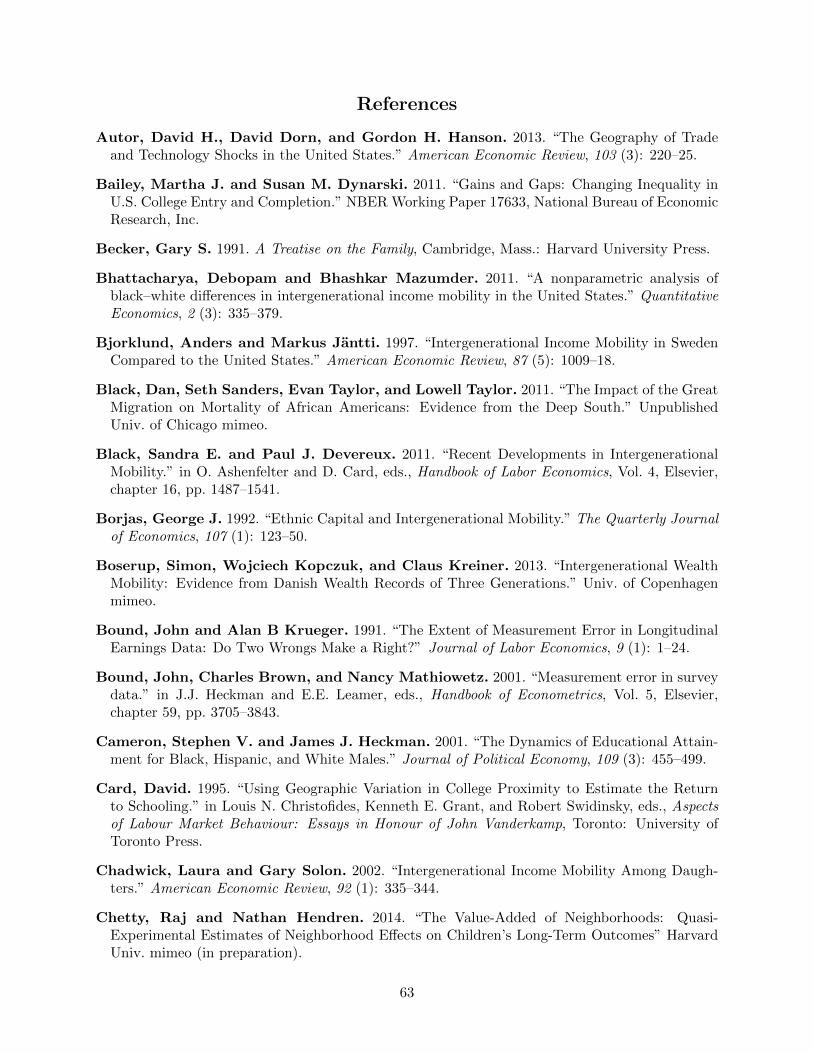
References

Autor, David H., David Dorn, and Gordon H. Hanson. 2013. “The Geography of Tradeand Technology Shocks in the United States.” American Economic Review, 103 (3): 220–25.

Bailey, Martha J. and Susan M. Dynarski. 2011. “Gains and Gaps: Changing Inequality inU.S. College Entry and Completion.” NBER Working Paper 17633, National Bureau of EconomicResearch, Inc.

Becker, Gary S. 1991. A Treatise on the Family, Cambridge, Mass.: Harvard University Press.

Bhattacharya, Debopam and Bhashkar Mazumder. 2011. “A nonparametric analysis ofblack–white differences in intergenerational income mobility in the United States.” QuantitativeEconomics, 2 (3): 335–379.

Bjorklund, Anders and Markus Jantti. 1997. “Intergenerational Income Mobility in SwedenCompared to the United States.” American Economic Review, 87 (5): 1009–18.

Black, Dan, Seth Sanders, Evan Taylor, and Lowell Taylor. 2011. “The Impact of the GreatMigration on Mortality of African Americans: Evidence from the Deep South.” UnpublishedUniv. of Chicago mimeo.

Black, Sandra E. and Paul J. Devereux. 2011. “Recent Developments in IntergenerationalMobility.” in O. Ashenfelter and D. Card, eds., Handbook of Labor Economics, Vol. 4, Elsevier,chapter 16, pp. 1487–1541.

Borjas, George J. 1992. “Ethnic Capital and Intergenerational Mobility.” The Quarterly Journalof Economics, 107 (1): 123–50.

Boserup, Simon, Wojciech Kopczuk, and Claus Kreiner. 2013. “Intergenerational WealthMobility: Evidence from Danish Wealth Records of Three Generations.” Univ. of Copenhagenmimeo.

Bound, John and Alan B Krueger. 1991. “The Extent of Measurement Error in LongitudinalEarnings Data: Do Two Wrongs Make a Right?” Journal of Labor Economics, 9 (1): 1–24.

Bound, John, Charles Brown, and Nancy Mathiowetz. 2001. “Measurement error in surveydata.” in J.J. Heckman and E.E. Leamer, eds., Handbook of Econometrics, Vol. 5, Elsevier,chapter 59, pp. 3705–3843.

Cameron, Stephen V. and James J. Heckman. 2001. “The Dynamics of Educational Attain-ment for Black, Hispanic, and White Males.” Journal of Political Economy, 109 (3): 455–499.

Card, David. 1995. “Using Geographic Variation in College Proximity to Estimate the Returnto Schooling.” in Louis N. Christofides, Kenneth E. Grant, and Robert Swidinsky, eds., Aspectsof Labour Market Behaviour: Essays in Honour of John Vanderkamp, Toronto: University ofToronto Press.

Chadwick, Laura and Gary Solon. 2002. “Intergenerational Income Mobility Among Daugh-ters.” American Economic Review, 92 (1): 335–344.

Chetty, Raj and Nathan Hendren. 2014. “The Value-Added of Neighborhoods: Quasi-Experimental Estimates of Neighborhood Effects on Children’s Long-Term Outcomes” HarvardUniv. mimeo (in preparation).

63

Chetty, Raj, John N. Friedman, and Jonah E. Rockoff. 2014 forthcoming. “Measuring theImpacts of Teachers II: Teacher Value-Added and Student Outcomes in Adulthood.” AmericanEconomic Review.

Chetty, Raj, Nathaniel Hendren, Patrick Kline, Emmanuel Saez, and Nicholas Turner.2014. “Is the United States Still a Land of Opportunity? Recent Trends in IntergenerationalMobility.” American Economic Review Papers and Proceedings, 104 (5): 141–147.

Cilke, James. 1998. “A Profile of Non-Filers.” U.S. Department of the Treasury, Office of TaxAnalysis Working Paper No. 78.

Clark, Gregory. 2014. The Son Also Rises: Surnames and the History of Social Mobility.

Coleman, James S. 1988. “Social Capital in the Creation of Human Capital.” American Journalof Sociology, 94, pp. S95–S120.

Corak, Miles. 2013. “Income Inequality, Equality of Opportunity, and Intergenerational Mobility.”Journal of Economic Perspectives, 27 (3): 79–102.

Corak, Miles and Andrew Heisz. 1999. “The Intergenerational Earnings and Income Mobilityof Canadian Men: Evidence from Longitudinal Income Tax Data.” Journal of Human Resources,34 (3): 504–533.

Cutler, David M. and Edward L. Glaeser. 1997. “Are Ghettos Good or Bad?” The QuarterlyJournal of Economics, 112 (3): 827–72.

Cutler, David M., Edward L. Glaeser, and Jacob L. Vigdor. 1999. “The Rise and Declineof the American Ghetto.” Journal of Political Economy, 107 (3): 455–506.

Dahl, Molly W. and Thomas DeLeire. 2008. The association between children’s earnings andfathers’ lifetime earnings: estimates using administrative data, University of Wisconsin-Madison,Institute for Research on Poverty.

Dorn, David. “Essays on Inequality, Spatial Interaction, and the Demand for Skills.” PhD dis-sertation, University of St. Gallen no. 3613, 2009.

Duncan, Greg J., Kathleen M. Ziol-Guest, and Ariel Kalil. 2010. “Early-Childhood Povertyand Adult Attainment, Behavior, and Health.” Child Development, 81 (1): 306–325.

Fields, Gary S. and Efe A. Ok. 1999. “The Measurement of Income Mobility: An Introductionto the Literature.” in Jacques Silber, ed., Handbook of Income Inequality Measurement, Vol. 71,Springer Netherlands, pp. 557–598.

Graham, Bryan and Patrick Sharkey. 2013. “Mobility and the Metropolis: How Communi-ties Factor Into Economic Mobility.” Washington D.C.: Economic Mobility Project, The PewCharitable Trusts.

Grawe, Nathan D. 2006. “Lifecycle bias in estimates of intergenerational earnings persistence.”Labour Economics, 13 (5): 551–570.

Haider, Steven and Gary Solon. 2006. “Life-Cycle Variation in the Association between Currentand Lifetime Earnings.” American Economic Review, 96 (4): 1308–1320.

Hanushek, Eric A. 2003. “The Failure of Input-Based Schooling Policies.” Economic Journal,113 (485): F64–F98.

64

Heckman, James J. 2006. “Skill Formation and the Economics of Investing in DisadvantagedChildren.” Science, 312 (5782): 1900–1902.

Hertz, Tom. 2006. “Understanding mobility in America.” Center for American Progress Discus-sion Paper.

Hotz, Joseph V. and John K. Scholz. “The Earned Income Tax Credit.” in Rober A. Moffitt,ed., Means-Tested Transfer Programs in the United States, University of Chicago Press 2003.pp. 141–197.

Iceland, John. 2004. “Beyond Black and White: Metropolitan residential segregation in multi-ethnic America.” Social Science Research, 33 (2): 248–271.

Internal Revenue Service. 2013. “Statistics of Income: Individual Income Tax Returns, 2012.”Technical Report, Washington, DC: government printing press.

Jencks, Christopher and Susan E. Mayer. 1990. “The Social Consequences of Growing Upin a Poor Neighborhood.” in L. Lynn and M. G. H. McGeary, eds., Inner City Poverty in theUnited States, Washington D.C.: National Academy Press, p. 111–186.

Jantti, Markus, Bernt Bratsberg, Knut Røed, Oddbjørn Raaum, Robin Naylor, EvaOsterbacka, Anders Bjorklund, and Tor Eriksson. 2006. “American Exceptionalism in aNew Light: A Comparison of Intergenerational Earnings Mobility in the Nordic Countries, theUnited Kingdom and the United States.” IZA Discussion Paper 1938, Institute for the Study ofLabor (IZA).

Kain, John F. 1968. “Housing Segregation, Negro Employment, and Metropolitan Decentraliza-tion.” The Quarterly Journal of Economics, 82 (2): 175–197.

Kasarda, John D. 1989. “Urban Industrial Transition and the Underclass.” Annals of the Amer-ican Academy of Political and Social Science, 501, pp. 26–47.

Katz, Lawrence F., Jeffrey R. Kling, and Jeffrey B. Liebman. 2001. “Moving To Opportu-nity In Boston: Early Results Of A Randomized Mobility Experiment.” The Quarterly Journalof Economics, 116 (2): 607–654.

Kline, Patrick and Andres Santos. 2013. “Sensitivity to missing data assumptions: Theoryand an evaluation of the U.S. wage structure.” Quantitative Economics, 4 (2): 231–267.

Kline, Patrick and Enrico Moretti. 2014. “People, Places and Public Policy: Some SimpleWelfare Economics of Local Economic Development Programs.” Annual Review of Economics, 6(1): forthcoming.

Krueger, Alan. “The Rise and Consequences of Inequality in the United States.” Speech at theCenter for American Progress, Washington D.C. on January 12, 2012.

Lamb, Michael E. 2004. The Role of the Father in Child Development, Hoboken, N.J.: Wiley.

Lee, Chul-In and Gary Solon. 2009. “Trends in Intergenerational Income Mobility.” The Reviewof Economics and Statistics, 91 (4): 766–772.

Massey, Douglas S and Nancy A Denton. 1993. American Apartheid: Segregation and theMaking of the Underclass, Cambridge, Mass.: Harvard University Press.

65

Mazumder, Bhashkar. 2005. “Fortunate Sons: New Estimates of Intergenerational Mobility inthe United States Using Social Security Earnings Data.” The Review of Economics and Statistics,87 (2): 235–255.

Mazumder, Bhashkar. 2011. “Black-white differences in intergenerational economic mobility inthe US.” Working Paper Series WP-2011-10, Federal Reserve Bank of Chicago.

Mitnik, Pablo, Victoria Bryant, David B. Grusky, and Michael Weber. 2014. “NewEstimates of Intergnerational Income Mobility Using Administrative Data.” Statistics of Income,Internal Revenue Service. mimeo (in preparation).

Murray, Charles A. 1984. Losing ground: American social policy, 1950-1980, New York: BasicBooks.

Murray, Charles A. 2012. Coming apart: the state of white America, 1960-2010, New York,N.Y.: Crown Forum.

Neal, Derek A and William R Johnson. 1996. “The Role of Premarket Factors in Black-WhiteWage Differences.” Journal of Political Economy, 104 (5): 869–95.

Oreopoulos, Philip. 2003. “The Long-Run Consequences of Living in a Poor Neighborhood.”The Quarterly Journal of Economics, 118 (4): 1533–1575.

Piketty, Thomas and Emmanuel Saez. 2003. “Income Inequality in the United States,1913–1998.” The Quarterly Journal of Economics, 118 (1): 1–41.

Putnam, Robert D. 1995. “Bowling Alone: America’s Declining Social Capital.” Journal ofDemocracy, 6 (1): 65–78.

Ray, Debraj. 2010. “Uneven Growth: A Framework for Research in Development Economics.”Journal of Economic Perspectives, 24 (3): 45–60.

Reardon, Sean and Kendra Bischoff. 2011. “Growth in the residential segregation of familiesby income, 1970–2009.” US 2010 Project.

Reardon, Sean F. 2011. “Measures of income segregation.” CEPA Working Papers. Stanford,CA: Stanford Center for Education Policy Analysis.

Reardon, Sean F. and Glenn Firebaugh. 2002. “Measures of Multigroup Segregation.” Soci-ological Methodology, 32 (1): 33–67.

Rupasingha, Anil and Stephan J. Goetz. 2008. “US County-Level Social Capital Data, 1990-2005.” The Northeast Regional Center for Rural Development, Penn State University, UniversityPark, PA.

Sampson, Robert J., Jeffrey D. Morenoff, and Thomas Gannon-Rowley. 2002. “Assessing“Neighborhood Effects”: Social Processes and New Directions in Research.” Annual Review ofSociology, 28 (1): 443–478.

Solon, Gary. 1992. “Intergenerational Income Mobility in the United States.” American EconomicReview, 82 (3): 393–408.

Solon, Gary. 1999. “Intergenerational Mobility in the Labor Market.” in O. Ashenfelter andD. Card, eds., Handbook of Labor Economics, Vol. 3, Elsevier, pp. 1761–1800.

66

Solon, Gary. 2002. “Cross-Country Differences in Intergenerational Earnings Mobility.” Journalof Economic Perspectives, 16 (3): 59–66.

Solon, Gary, Marianne E. Page, and Greg J. Duncan. 2000. “Correlations Between Neigh-boring Children In Their Subsequent Educational Attainment.” The Review of Economics andStatistics, 82 (3): 383–392.

Theil, Henri. 1972. Statistical decomposition analysis. With applications in the social and ad-ministrative sciences number v. 14. In ‘Studies in mathematical and managerial economics.’,Amsterdam, New York: North-Holland Pub. Co.; American Elsevier Pub. Co.

Thomas, Adam and Isabel Sawhill. 2002. “For richer or for poorer: Marriage as an antipovertystrategy.” Journal of Policy Analysis and Management, 21 (4): 587–599.

Tolbert, Charles M. and Molly Sizer. 1996. “U.S. Commuting Zones and Labor Market Areas:A 1990 update.” Economic Research Service Staff Paper, 9614.

Trivedi, Pravin K. and David M. Zimmer. 2007. “Copula Modeling: An Introduction forPractitioners.” Foundations and Trends in Econometrics, 1 (1): 1–111.

Wilson, William J. 1987. The truly disadvantaged: the inner city, the underclass, and publicpolicy, Chicago: University of Chicago Press.

Wilson, William J. 1996. When work disappears: the world of the new urban poor, New York:Knopf: Distributed by Random House, Inc.

Zimmerman, David J. 1992. “Regression toward Mediocrity in Economic Stature.” AmericanEconomic Review, 82 (3): 409–29.

67

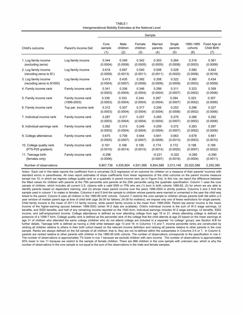
Child's outcome Parent's Income Def.Core

sampleMale

childrenFemale children

Married parents

Single parents

1980-1985 cohorts

Fixed Age at Child Birth

(1) (2) (3) (4) (5) (6) (7)

1. Log family income Log family income 0.344 0.349 0.342 0.303 0.264 0.316 0.361 (excluding zeros) (0.0004) (0.0006) (0.0005) (0.0005) (0.0008) (0.0003) (0.0008)

2. Log family income Log family income 0.618 0.697 0.540 0.509 0.528 0.580 0.642 (recoding zeros to $1) (0.0009) (0.0013) (0.0011) (0.0011) (0.0020) (0.0006) (0.0018)

3. Log family income Log family income 0.413 0.435 0.392 0.358 0.322 0.380 0.434 (recoding zeros to $1000) (0.0004) (0.0007) (0.0006) (0.0006) (0.0009) (0.0003) (0.0009)

4. Family income rank Family income rank 0.341 0.336 0.346 0.289 0.311 0.323 0.359(0.0003) (0.0004) (0.0004) (0.0004) (0.0007) (0.0002) (0.0006)

5. Family income rank Family income rank 0.339 0.333 0.344 0.287 0.294 0.323 0.357(1999-2003) (0.0003) (0.0004) (0.0004) (0.0004) (0.0007) (0.0002) (0.0006)

6. Family income rank Top par. income rank 0.312 0.307 0.317 0.256 0.253 0.296 0.327(0.0003) (0.0004) (0.0004) (0.0004) (0.0006) (0.0002) (0.0006)

7. Individual income rank Family income rank 0.287 0.317 0.257 0.265 0.279 0.286 0.292(0.0003) (0.0004) (0.0004) (0.0004) (0.0007) (0.0002) (0.0006)

8. Individual earnings rank Family income rank 0.282 0.313 0.249 0.259 0.272 0.283 0.287(0.0003) (0.0004) (0.0004) (0.0004) (0.0007) (0.0002) (0.0006)

9. College attendance Family income rank 0.675 0.708 0.644 0.641 0.663 0.678 0.661(0.0005) (0.0007) (0.0007) (0.0006) (0.0013) (0.0003) (0.0010)

10. College quality rank Family income rank 0.191 0.188 0.195 0.174 0.172 0.198 0.189 (P75-P25 gradient) (0.0010) (0.0014) (0.0015) (0.0014) (0.0020) (0.0007) (0.0022)

11. Teenage birth Family income rank -0.298 -0.231 -0.322 -0.285 -0.290 (females only) (0.0006) (0.0007) (0.0016) (0.0004) (0.0011)

Number of observations 9,867,736 4,935,804 4,931,066 6,854,588 3,013,148 20,520,588 2,250,380

Sample

Intergenerational Mobility Estimates at the National LevelTABLE I

Notes: Each cell in this table reports the coefficient from a univariate OLS regression of an outcome for children on a measure of their parents' incomes withstandard errors in parentheses. All rows report estimates of slope coefficients from linear regressions of the child outcome on the parent income measureexcept row 10, in which we regress college quality rank on a quadratic in parent income rank (as in Figure IVa). In this row, we report the difference betweenthe fitted values for children with parents at the 75th percentile and parents at the 25th percentile using the quadratic specification. Column 1 uses the coresample of children, which includes all current U.S. citizens with a valid SSN or ITIN who are (1) born in birth cohorts 1980-82, (2) for whom we are able toidentify parents based on dependent claiming, and (3) whose mean parent income over the years 1996-2000 is strictly positive. Columns 2 and 3 limit thesample used in column 1 to males or females. Columns 4 and 5 limit the sample to children whose parents were married or unmarried in the year the child waslinked to the parent. Column 6 uses all children in the 1980-85 birth cohorts. Column 7 restricts the core sample to children whose parents both fall within a 5year window of median parent age at time of child birth (age 26-30 for fathers; 24-28 for mothers); we impose only one of these restrictions for single parents.Child family income is the mean of 2011-12 family income, while parent family income is the mean from 1996-2000. Parent top earner income is the meanincome of the higher-earning spouse between 1999-2003 (when W-2 data are available). Child's individual income is the sum of W-2 wage earnings, UIbenefits, and SSDI benefits, and half of any remaining income reported on the 1040 form. Individual earnings includes W-2 wage earnings, UI benefits, SSDIincome, and self-employment income. College attendance is defined as ever attending college from age 18 to 21, where attending college is defined aspresence of a 1098-T form. College quality rank is defined as the percentile rank of the college that the child attends at age 20 based on the mean earnings atage 31 of children who attended the same college (children who do not attend college are included in a separate “no college” group); see Section III.B forfurther details. Teenage birth is defined as having a child while between age 13 and 19. In Columns 1-5 and 7, income percentile ranks are constructed byranking all children relative to others in their birth cohort based on the relevant income definition and ranking all parents relative to other parents in the coresample. Ranks are always defined on the full sample of all children; that is, they are not re-defined within the subsamples in Columns 2-5 or 7. In Column 6,parents are ranked relative to other parents with children in the 1980-85 birth cohorts. The number of observations corresponds to the specification in row 4.The number of observations is approximately 7% lower in row 1 because we exclude children with zero income. The number of observations is approximately50% lower in row 11 because we restrict to the sample of female children. There are 866 children in the core sample with unknown sex, which is why thenumber of observations in the core sample is not equal to the sum of the observations in the male and female samples.

1 2 3 4 51 33.7% 24.2% 17.8% 13.4% 10.9%2 28.0% 24.2% 19.8% 16.0% 11.9%3 18.4% 21.7% 22.1% 20.9% 17.0%4 12.3% 17.6% 22.0% 24.4% 23.6%5 7.5% 12.3% 18.3% 25.4% 36.5%

Parent Quintile

Child Quintile

Notes. Each cell reports the percentage of children with family income inthe quintile given by the row conditional on having parents with familyincome in the quintile given by the column for the 9,867,736 children in thecore sample (1980-82 birth cohorts). See notes to Table I for income andsample definitions. See Online Appendix Table VI for an analogoustransition matrix constructed using the 1980-85 cohorts.

TABLE IINational Quintile Transition Matrix

CZ Name Population(1) (2) (3) (4) (5) (6) (7)1 Salt Lake City, Utah 1,426,729 46.2 10.8 77.3 0.2642 Pittsburgh, Pennsylvania 2,561,364 45.2 9.5 74.9 0.3593 San Jose, California 2,393,183 44.7 12.9 73.5 0.2354 Boston, Massachusetts 4,974,945 44.6 10.5 73.7 0.3225 San Francisco, California 4,642,561 44.4 12.2 72.5 0.2506 San Diego, California 2,813,833 44.3 10.4 74.3 0.2377 Manchester, New Hampshire 1,193,391 44.2 10.0 75.0 0.2968 Minneapolis, Minnesota 2,904,389 44.2 8.5 75.2 0.3389 Newark, New Jersey 5,822,286 44.1 10.2 73.7 0.350

10 New York, New York 11,781,395 43.8 10.5 72.2 0.33011 Los Angeles, California 16,393,360 43.4 9.6 73.8 0.23112 Providence, Rhode Island 1,582,997 43.4 8.2 73.6 0.33313 Washington DC 4,632,415 43.2 11.0 72.2 0.33014 Seattle, Washington 3,775,744 43.2 10.9 72.0 0.27315 Houston, Texas 4,504,013 42.8 9.3 74.7 0.32516 Sacramento, California 2,570,609 42.7 9.7 71.3 0.25717 Bridgeport, Connecticut 3,405,565 42.4 7.9 72.4 0.35918 Fort Worth, Texas 1,804,370 42.3 9.1 73.6 0.32019 Denver, Colorado 2,449,044 42.2 8.7 73.3 0.29420 Buffalo, New York 2,369,699 42.0 6.7 73.1 0.36821 Miami, Florida 3,955,969 41.5 7.3 76.3 0.26722 Fresno, California 1,419,998 41.3 7.5 71.3 0.29523 Portland, Oregon 1,842,889 41.3 9.3 70.5 0.27724 San Antonio, Texas 1,724,863 41.1 6.4 74.3 0.32025 Philadelphia, Pennsylvania 5,602,247 40.8 7.4 69.6 0.39326 Austin, Texas 1,298,076 40.4 6.9 71.9 0.32327 Dallas, Texas 3,405,666 40.4 7.1 72.6 0.34728 Phoenix, Arizona 3,303,211 40.3 7.5 70.6 0.29429 Grand Rapids, Michigan 1,286,045 40.1 6.4 71.3 0.37830 Kansas City, Missouri 1,762,873 40.1 7.0 70.4 0.36531 Las Vegas, Nevada 1,568,418 40.0 8.0 71.1 0.25932 Chicago, Illinois 8,183,799 39.4 6.5 70.8 0.39333 Milwaukee, Wisconsin 1,660,659 39.3 4.5 70.3 0.42434 Tampa, Florida 2,395,997 39.1 6.0 71.3 0.33535 Orlando, Florida 1,697,906 39.1 5.8 71.5 0.32636 Port St. Lucie, Florida 1,533,306 39.0 6.2 71.2 0.30337 Baltimore, Maryland 2,512,431 38.8 6.4 67.7 0.41238 St. Louis, Missouri 2,325,609 38.4 5.1 69.0 0.41339 Dayton, Ohio 1,179,009 38.3 4.9 68.2 0.39740 Cleveland, Ohio 2,661,167 38.2 5.1 68.7 0.40541 Nashville, Tennessee 1,246,338 38.2 5.7 67.9 0.35742 New Orleans, Louisiana 1,381,652 38.2 5.1 69.5 0.39743 Cincinnati, Ohio 1,954,800 37.9 5.1 66.4 0.42944 Columbus, Ohio 1,663,807 37.7 4.9 67.1 0.40645 Jacksonville, Florida 1,176,696 37.5 4.9 68.9 0.36146 Detroit, Michigan 5,327,827 37.3 5.5 68.5 0.35847 Indianapolis, Indiana 1,507,346 37.2 4.9 67.5 0.39848 Raleigh, North Carolina 1,412,127 36.9 5.0 67.3 0.38949 Atlanta, Georgia 3,798,017 36.0 4.5 69.4 0.36650 Charlotte, North Carolina 1,423,942 35.8 4.4 67.0 0.397

Notes: This table reports estimates of intergenerational mobility for the 50 largest commuting zones (CZs) according to their populations in the 2000Census. The CZs are sorted in descending order by absolute upward mobility (Column 4). The mobility measures are calculated using the coresample (1980-82 birth cohorts) and the baseline family income definitions described in Table I (except for Column 5, which uses the 1980-85 birthcohorts). The measures in Columns 4 and 7 are both derived from within-CZ OLS regressions of child income rank against parent income rank.Column 7 reports the slope coefficient from this regression, which is equal to the difference in mean child income rank between children with parentsin the 100th percentile and children with parents in the 0th percentile (divided by 100). Column 4 reports the predicted value at parent income rankequal to 25. Column 5 reports the percentage of children whose family income is in the top quintile of the national distribution of child family incomeconditional on having parent family income in the bottom quintile of the parental national income distribution. These probabilities are taken directlyfrom Online Data Table VII. Column 6 reports the fitted values at parent rank 25 from a regression of an indicator for child family income being abovethe poverty line on parent income rank (see Appendix F for details). . See Online Data Table V for estimates for all CZs as well as estimates usingalternative samples and income definitions.

TABLE III

Relative Mobility Rank-Rank Slope

P(Child in Q5 | Parent in Q1)

Upward Mob. Rank

Absolute Upward Mobility

Intergenerational Mobility in the 50 Largest Commuting Zones

Pct. Above Poverty Line

Dep. Var.:(1) (2) (3) (4) (5) (6) (7)

Racial Segregation -0.361 -0.360(0.045) (0.068)

Income Segregation -0.393 -0.058(0.065) (0.090)

Segregation of Poverty (<p25) -0.508 -0.408(0.155) (0.166)

Segregation of Affluence (>p75) 0.108 0.216(0.140) (0.171)

Share with Commute < 15 Mins 0.605 0.571(0.126) (0.165)

Urban Areas Only x xR-Squared 0.131 0.130 0.154 0.167 0.052 0.366 0.368Observations 709 325 709 709 325 709 709

TABLE IVSegregation and Intergenerational Mobility

Notes: Each column reports coefficients from an OLS regression with standard errors clustered at the state level reportedin parentheses. All independent and dependent variables are normalized (in the relevant estimation sample) to have mean0 and standard deviation 1, so univariate regression coefficients equal correlation coefficients. The regressions are runusing data for the 709 CZs with at least 250 children in the core sample. The dependent variable in all columns is ourbaseline measure of absolute upward mobility, the expected rank of children whose parents are at the 25th nationalpercentile. Column 2 and 5 restrict to the sample of CZs that intersect an MSA. Racial segregation is measured by theTheil index defined in Section VI.B using racial shares at the census tract level. Income segregation is measured by aweighted average of two-group Theil indices, as in Reardon (2011). Segregation of poverty is a two-group Theil index,where the groups are defined as being above vs. below the 25th percentile of the local household income distribution.Segregation of affluence is defined analogously at the 75th percentile. Share with commute <15 minutes is the fraction ofworking individuals in each CZ who commute less than 15 minutes to work. See Appendix G for details on the definitionsof the independent variables.

Absolute Upward Mobility

Dep. Var.: Log-LogElasticity

2005 Inequality(1) (2) (3) (4) (5) (6) (7) (8)

Gini Coefficient -0.578(0.093)

Gini Bottom 99% -0.634 -0.624 0.476 0.72 0.62 0.78(0.090) (0.113) (0.088) (0.21) (0.27) (0.27)

Top 1% Income Share -0.123 0.029 -0.032 0.17 -0.11(0.035) (0.039) (0.032) (0.27) (0.28)

Frac. Between p25 and p75 0.679(0.111)

Urban Areas Only x

R-Squared 0.334 0.433 0.380 0.462 0.224 0.518 0.536 0.531

Observations 709 709 325 709 709 13 13 12

Notes: Each column reports regression coefficients from an OLS regression with all variables normalized to have mean 0 and standarddeviation 1 in the estimation sample, so univariate regression coefficients are equal to correlation coefficients. Columns 1-5 are estimatedusing data for the 709 CZs with at least 250 children in the core sample. The dependent variable in Columns 1-4 is our baseline CZ-levelmeasure of absolute upward mobility, the expected rank of children whose parents are at the 25th national percentile in the core sample. InColumn 5, the dependent variable is relative mobility, the rank-rank slope within each CZ. In Column 3, we restrict to CZs that intersectMSAs. In Columns 1-5, the Gini coefficient is defined as the Gini coefficient of family income for parents in the core sample in each CZ; thetop 1% income share is defined as the fraction of total parent family income in each CZ accruing to the richest 1% of parents in that CZ; theGini Bottom 99% is defined as the Gini coefficient minus the top 1% income share; and the fraction between p25 and p75 is the fraction ofparents in each CZ whose family income is between the 25th and 75th percentile of the national distribution of parent family income forthose in the core sample. In Columns 6-8, the dependent variable is the log-log IGE estimate by country from Corak (2013, Figure 1). TheGini coefficients across countries are obtained from the OECD Income Distribution Database (series "Income Distribution and Poverty: bycountry"). We interpret these coefficients as applying to the bottom 99% because the surveys on which they are based are typically top-coded. The top 1% income share across countries is from the World Top Income Database (series "Top 1% Income Share"). Theindependent variables are measured in 1985 in Columns 6 and 7 and in 2005 in Column 8.

Across Countries

TABLE VIncome Inequality and Intergenerational Mobility: The "Great Gatsby" Curve

Across CZs within the U.S.Log-LogElasticityRelative

MobilityAbsolute Upward Mobility1985 Inequality

Dep. Var.:(1) (2) (3) (4) (5) (6) (7) (8)

Fraction Short Commute 0.302 0.227 0.314 -0.290 -0.325 0.331 0.319(0.065) (0.077) (0.052) (0.061) (0.064) (0.070) (0.065)

Gini Bottom 99% -0.009 -0.017 0.060 0.006 0.343 -0.287 -0.021(0.053) (0.043) (0.097) (0.071) (0.095) (0.059) (0.054)

High School Dropout Rate -0.147 -0.120 -0.109 0.010 0.181 -0.288 -0.140(0.055) (0.038) (0.085) (0.064) (0.056) (0.059) (0.055)

Social Capital Index 0.169 0.065 0.173 0.154 0.154 0.168 0.168(0.047) (0.050) (0.060) (0.060) (0.070) (0.059) (0.045)

Fraction Single Mothers -0.487 -0.477 -0.555 0.591 -0.808 -0.579(0.062) (0.071) (0.089) (0.049) (0.085) (0.061)

Fraction Black 0.056 0.132(0.073) (0.051)

State Fixed Effects x

Urban Areas Only x

R-Squared 0.757 0.859 0.671 0.48 0.324 0.651 0.584 0.763

Observations 709 709 325 709 709 709 709 709

Notes: Each column reports coefficients from an OLS regression with standard errors clustered at the state level reported inparentheses. The regressions are run using data for the 709 CZs with at least 250 children in the core sample. The dependentvariable in Columns 1-3 and 6-8 is our baseline measure of absolute upward mobility, the expected rank of children whoseparents are at the 25th national percentile. The dependent variable in columns 4 and 5 is relative mobility, the rank-rank slopewithin each CZ. All independent and dependent variables are normalized (in the relevant estimation sample) to have mean 0 andstandard deviation 1. Column 1 reports unweighted estimates across all CZs. Column 2 includes state fixed effects. In Column 3,we restrict to CZs that intersect MSAs. Columns 4-8 replicate the unweighted specification in Column 1 with different dependentand independent variables. The fraction with short commutes is the share of workers that commute to work in less than 15minutes calculated using data for the 2000 Census. Gini bottom 99% is the Gini coefficient minus the top 1% income share withineach CZ, computed using the distribution of parent family income within each CZ for parents in the core sample. Income-residualized high school dropout rate is the residual from a regression of the fraction of children who drop out of high school inthe CZ, estimated using data from the NCES Common Core of Data for the 2000-01 school year, on mean household income in2000. Social capital index is the standardized index of social capital constructed by Rupasingha and Goetz (2008). Fractionsingle mothers is the fraction of children being raised by single mothers in each CZ. Fraction black is the number of people in theCZ who are black alone divided by the CZ population. We code the high school dropout rate as 0 for 116 CZs in which dropoutrate data are missing for more than 25% of the districts in the CZ, and include an indicator for having a missing high schooldropout rate. We do the same for 16 CZs with missing data on social capital. See Section VI, Online Data Table IX, and OnlineAppendix G for additional details on the definitions of each of these variables.

Correlates of Intergenerational Mobility: Comparing Alternative Hypotheses TABLE VI

Relative Mobility Absolute Upward MobilityAbsolute Upward Mobility

Base national dataset

Base CZ-level dataset

Size of Birth Cohort

(in '000s)

Percentage in DM1 database,

US citizens, alive

and matched to a parent

with positive parent income in 1996-2000

and with valid parental geo information

(1) (2) (3) (4) (5)1977 3,327 95.9% 55.0%1978 3,333 97.0% 72.4%1979 3,494 97.6% 80.9%1980 3,612 99.2% 85.6% 85.2% 84.4%1981 3,629 104.6% 91.6% 91.1% 90.3%1982 3,681 105.5% 93.8% 93.2% 92.4%1983 3,639 105.4% 95.4% 94.7% 93.8%1984 3,669 105.1% 96.7% 95.8% 94.9%1985 3,761 104.8% 97.5% 96.4% 95.4%1986 3,757 104.7% 98.0% 96.6% 95.6%1987 3,809 104.7% 98.4% 96.8% 95.8%1988 3,910 104.5% 98.5% 96.8% 95.7%1989 4,041 105.0% 98.5% 96.7% 95.6%1990 4,158 104.7% 98.6% 96.7% 95.6%1991 4,111 104.5% 98.5% 96.6% 95.5%1980-1991 45,776 104.4% 96.0% 94.8% 93.8%

ONLINE APPENDIX TABLE ISample Sizes vs. Vital Statistics Counts by Birth Cohort

Notes: Column 1 reports the size of each birth cohort from 1987-1991, based on data from vitalstatistics obtained from the US Statistical Abstract 2012, Table 78. The remaining columns reportthe number of individuals in the population tax data as a percentage of the total number in thebirth cohort, imposing the additional restrictions listed in the header of each column. Column 2reports the number of individuals born in each cohort who are in the DM1 tax database, arecurrent US citizens, and are alive in 2013. This column can differ from the birth cohort due toimmigration and naturalization, emigration, and deaths before 2012. The percentage of citizens inthe DM1 data rises in 1981 because citizenship status is missing for some individuals born before1981. Column 3 further requires the individuals to be matched to parents (i.e., claimed as childrendependents on individual income tax returns by a person aged 15-40 at the time of the birth of thechild) in 1996 or after. Column 4, which requires in addition that parents have positive meanincome between 1996-2000, is our key sample of interest for all national level statistics. Column 5further requires valid geographical information (ZIP code) for parents. Column 5 is our key sampleof interest for all local area statistics. The core sample includes the 1980-2 cohorts. The extendedsample includes the 1980-91 cohorts.

Number of Observations Number of Unique ChildrenCohort (1) (2)1971 4,383 4,3831972 7,787 5,5691973 10,831 6,1541974 14,330 7,0651975 17,736 8,2071976 17,938 8,2461977 18,459 8,1561978 17,756 7,9581979 18,375 7,6141980 19,545 7,7321981 19,916 8,1551982 22,331 9,9291983 24,599 10,9271984 28,221 12,3901985 31,711 13,4761986 33,221 13,5401987 35,382 14,2341988 38,139 15,3621989 42,450 18,1621990 47,768 19,8051991 52,821 21,231Total 523,699 228,295

ONLINE APPENDIX TABLE IISOI Sample Counts by Birth Cohort

Notes: This table reports the sample size for the Statistics of Income stratifiedrandom sample by birth cohort. Column 1 reports the total number of observationsper cohort. Column 2 reports the number of unique children per cohort. SeeAppendix A for details on the construction of the SOI sample.

Variable Mean Std. Dev. Median(1) (2) (3)

Parents: Family Income (1996-2000 average) 87,219 353,430 60,129 Top Earner's Income (1999-2003 average) 68,854 830,487 48,134 Fraction Single Parents 30.6% 46.1% Fraction Female among Single Parents 72.0% 44.9% Father's Age at Child Birth 28.5 6.2 28 Mother's Age at Child Birth 26.1 5.2 26 Father's Age in 1996 43.5 6.3 43 Mother's Age in 1996 41.1 5.2 41

Children: Family Income (2011-12 average) 48,050 93,182 34,975 Fraction with Zero Family Income 6.1% 23.9% Individual Income 31,441 112,394 24,931 Individual Earnings 30,345 98,692 23,811 Fraction Female 50.0% 50.0% Fraction Single 44.3% 49.7% Attend College between 18-21 58.9% 49.2% Fraction of Females with Teen Birth 15.8% 36.5% Child's Age in 2011 30.0 0.8 30

Number of Children

ONLINE APPENDIX TABLE IIISummary Statistics for Core Sample: Children Born in 1980-82

9,867,736

Notes: The table presents summary statistics for the core sample (1980-82 birth cohorts); see notes toTable I for further details on the definition of the core sample. Child income is mean income in 2011-12(when the child is approximately 30 years old), while parent family income is mean income from 1996-2000. Family income is total pre-tax household income. Top earner's income is the income of the higher-earning parent from 1999-2003 (when W-2's are available). Parents' marital status is measured in theyear the parent is matched to the child. Child's individual income is the sum of W-2 wage earnings, UIbenefits, and SSDI benefits, and half of any remaining income reported on the 1040 form. Individualearnings includes W-2 wage earnings, UI benefits, SSDI income, and self-employment income. A child isdefined as single if he/she does not file with a spouse in 2011 and 2012. College attendance is defined asever attending college from age 18 to 21, where attending college is defined as presence of a 1098-Tform. Teenage birth is defined (for females only) as having a child while being aged 19 or less. SeeSection III.B and Online Appendix A for additional details on sample and variable definitions. All dollarvalues are reported in 2012 dollars, deflated using the CPI-U.

Tax Data Full Sample

Tax Data Core Sample

2011-2012 CPS

2011-2012 ACS

Tax Data Full Sample

Tax Data Core Sample

2011-2012 CPS

2011-2012 ACS

(1) (2) (3) (4) (5) (6) (7) (8)

Income Distribution:

% Zero 9.74% 7.32% 9.23% 12.64% 8.54% 6.11% 5.44% 8.00% % Negative 0.00% 0.00% 0.00% 0.00% 0.33% 0.34% 0.04% 0.05% Mean 44,278 46,805 54,313 42,382 45,406 48,050 56,438 44,845 Std. Deviation 104,528 109,667 58,556 47,879 90,594 93,182 59,145 50,072 P10 63 1,624 1,307 0 521 2,810 6,431 1,500 P25 12,724 14,984 18,843 12,000 12,842 14,919 20,414 14,000 P50 32,165 34,737 40,829 31,642 32,273 34,975 42,768 33,000 P75 62,095 65,148 75,000 57,000 62,992 66,169 76,554 60,000 P90 96,995 99,911 115,000 91,865 98,802 101,770 118,050 96,243

Demographics:

% Married 42.43% 44.31% 49.32% 46.17% % Female 50.03% 49.97% 50.43% 49.98% % Live in South 36.83% 37.94% 38.33% 37.56% % College 54.62% 58.93% 66.20% 61.34%

Observations 11,262,459 9,867,736 14,246 190,561 11,262,459 9,867,736 14,246 194,501Sum of Samp. Weights 11,262,459 9,867,736 10,845,147 11,043,039 11,262,459 9,867,736 10,845,147 11,043,039

ONLINE APPENDIX TABLE IVComparison of Administrative Tax Data to CPS and ACS Survey Datasets

Earned Family Income Total Family Income

Notes: Columns (1) and (5) include all individuals in the Data Master-1 file from the SSA who were born in 1980-1982, are current U.S. citizens, andlived through 2012. In Columns (2) and (6), we impose the additional restriction that an individual was claimed as a dependent on a tax return in theyears 1996-2012 by parents with positive income as described in the text. CPS sample consists of civilian, non-institutionalized citizens age 29-31 inthe 2011 wave and 30-32 in 2012 waves of the Current Population Survey. ACS sample consists of civilian, non-institutionalized citizens born between1980-1982 in the 2011 and 2012 American Community Surveys. Earned income refers to wages and salary plus social security and unemploymentinsurance plus positive self-employment income, except for the ACS measure, which does not include unemployment insurance. IRS wages andsalary income is defined as the amount of all wages, tips, and other compensation before any payroll deductions (total of all amounts reported on allForms W-2, Box 1). IRS unemployment compensation is defined as the amount of Unemployment Compensation and Railroad Retirement Boardpayments prior to tax withholding as reported on Form 1099-G, Box 1. IRS social security income is defined as total Social Security Administrationbenefits, as reported on Form SSA-1099 (as well as any Railroad Retirement Board benefits paid, as reported on Form RRB-1099, Box 3). IRS self-employment income is defined as the profit reported on Form 1040 Schedule C. In the CPS, self-employment income is business income; in the ACS,it is both farm and non-farm business income. In the tax data, total income is the sum of Adjusted Gross Income, social security, and tax exemptinterest. Total income in CPS and ACS is all reported income including negative business and investment income. All dollar amounts are in 2012dollars. Married refers to filing of joint return in 2011-2012 period for the tax data, and self-report of currently married in CPS/ACS samples. Collegemeans attended a degree granting institution between the ages of 18 and 21 in the tax data and self-report of more than high school attainment inCPS/ACS samples. South refers to filing a federal tax return in (for tax data) or being surveyed in (for ACS/CPS) one of the following states: DE, DC,FL, GA, MD, NC, SC, VA, WV, AL, KY, MS, TN, AR, LA, OK, TX. ACS and CPS moments computed using sampling weights (inverse probability ofinclusion in sample). For the ACS and CPS, the sum of the sample weights is the average of the sum of the sample weights in 2011 and in 2012.

Name Freq. Number of NumberRestriction Children of Names Surname Individual Surname Individual

(1) (2) (3) (4) (5) (6)

1. No restriction 4,843,629 395,439 0.39 0.30 0.42 0.332. < 25 1,135,624 375,753 0.30 0.27 0.33 0.303. < 50 1,437,280 384,576 0.31 0.27 0.34 0.304. < 100 1,784,635 389,611 0.33 0.28 0.36 0.315. > 100 3,053,494 5,773 0.46 0.31 0.50 0.336. > 1,000 1,650,583 546 0.41 0.31 0.43 0.347. > 10,000 390,187 22 0.41 0.33 0.45 0.358. > 20,000 202,734 7 0.75 0.34 0.81 0.36

Rank-Rank Slope Log-Log IGE

ONLINE APPENDIX TABLE V

Notes: This table compares estimates of rank-rank slopes and log-log IGEs based on individual-level data to estimatesbased on surname means, as in Clark (2014). In this table, we restrict the core sample to children who have the samesurname (in 2012) as their parents. The first row uses all children who satisfy this restriction. Rows 2-4 limit the sample torare surnames: those that occur less than 25 times, 50 times, and 100 times in the sample. Conversely, rows 5-8 limit thesample to common surnames: those that occur more than 100, 1000, 10,000, and 20,000 times. Column 1 shows thenumber of children in each subsample (i.e., the number of observations used to estimate the rank-rank slope). Column 2shows the number of distinct surnames in each sample. We estimate the individual-level rank-rank slopes and log-logIGE's (Columns 4 and 6) using OLS regressions on the microdata as in Table I. In Columns 3 and 5, we estimate the rank-rank slopes and log-log IGE's using OLS regressions on a dataset collapsed to surname-level means, weighting by thenumber of observations for each name. See Appendix D for further details.

Estimates of Intergenerational Mobility Using Surname Means vs. Individual Incomes

1st 2nd 3rd 4th 5th1 33.1% 24.1% 17.7% 13.5% 11.7%2 27.7% 24.0% 19.6% 16.1% 12.6%3 18.7% 21.6% 21.9% 20.7% 17.0%4 12.7% 17.7% 21.8% 24.1% 23.7%5 7.8% 12.6% 18.9% 25.6% 35.1%

Notes. Each cell reports the percentage of children with family income in the quintile given by the rowconditional on having parents with family income in the quintile given by the column for children in the1980-85 birth cohorts. See notes to Table I for income and sample definitions. See Table II for ananalogous transition matrix constructed using the 1980-82 birth cohorts.

Child Quintile

ONLINE APPENDIX TABLE VINational Quintile Transition Matrix: 1980-85 Cohorts

Parent Quintile

Upward mobility Relative mobility Upward mobility Relative mobilityChange from Baseline Specification Unweighted Unweighted Pop. Weighted Pop. Weighted

(1) (2) (3) (4)

1. Male children 0.99, 1.07 0.94, 1.03 0.98, 1.07 0.98, 1.012. Female children 0.98, 0.96 0.95, 1.09 0.97, 0.98 0.98, 1.023. Children of married parents 0.97, 0.96 0.89, 0.92 0.91, 1.02 0.93, 0.894. Children of single parents 0.97, 0.97 0.61, 1.14 0.97, 0.96 0.83, 1.025. Birth cohorts 1983-85 0.97, 1.00 0.84, 1.08 0.96, 0.93 0.96, 1.056. Birth cohorts 1986-88 0.94, 0.95 0.73, 1.11 0.82, 0.91 0.88, 0.987. Parent age at child birth within 5 years of median 0.98, 1.06 0.90, 1.16 0.98, 1.05 0.96, 1.028. Children who stay within CZ 0.94, 1.02 0.87, 1.09 0.93, 1.12 0.95, 1.049. Children matched to unique parents 0.99, 0.93 0.98, 0.90 0.98, 0.93 0.99, 0.93

10. Top parent income 1.00, 1.05 0.97, 1.00 0.99, 1.04 0.99, 0.9911. Individual child income 0.94, 0.74 0.89, 0.80 0.83, 0.97 0.95, 0.8112. Individual child earnings 0.93, 0.72 0.86, 0.82 0.82, 0.93 0.93, 0.8213. Individual child income (males only) 0.96, 1.03 0.90, 1.01 0.96, 1.14 0.95, 0.9714. Indiv child income and top parent income (males only) 0.97, 1.07 0.87, 1.02 0.97, 1.15 0.94, 0.9515. Parent Income 1999-2003 1.00, 0.99 0.98, 0.99 1.00, 0.98 1.00, 0.99

16. Cost of living adjusted income 0.98, 1.06 0.99, 0.99 0.86, 1.01 0.99, 0.9717. Parent income measured in 2011/12 0.97, 0.90 0.92, 0.89 0.94, 0.95 0.98, 0.9318. Controlling for growth 0.83, 0.83 0.92, 0.92 0.81, 0.83 0.96, 0.97

19. Within-CZ ranks 0.95, 0.94 0.96, 0.9820. Prob. Child in Q5 | Parent in Q1 0.91 0.9221. Child income > poverty line 0.94 0.89

22. College Attendance (age 18-21) 0.71 0.68 0.53 0.7223. College Quality (age 20) 0.71 0.51 0.55 0.6524. Teenage Birth, females only -0.61 -0.58 -0.64 -0.68

Correlation with Baseline Mobility Estimates and Ratio of Std. Dev.

Robustness of Spatial Variation in Intergenerational Mobility to Alternative SpecificationsONLINE APPENDIX TABLE VII

Notes: The first number in each cell of this table reports the correlation across CZs of a baseline mobility measure (using child family income rankand parent family income rank in the core sample) with an alternative mobility measure. The second number in each cell reports the ratio of thestandard deviation of the alternative measure to the baseline measure. We do not report the ratio of standard deviations for statistics that aremeasured in different units relative to the corresponding baseline measure. The alternative mobility measures are defined either using a differentsample (Panel A), a different income measure for parents or children (Panel B), adjusting for cost of living or local growth (Panel C), using alternativestatistics for mobility (Panel D), or using earlier outcomes (Panel E). Column (1) reports the unweighted correlation (and SD ratio) between thealternative and baseline measure of absolute upward mobility, the expected rank of children whose parents are at the 25th national percentile in thecore sample. Column (2) reports the unweighted correlation (and SD ratio) between the alternative and baseline measure of relative mobility, theslope of the rank-rank relationship in the core sample. Columns (3) and (4) repeat Columns (1) and (2), weighting the correlations and standarddeviations by CZ population as recorded in the 2000 Census. With the exception of the transition probability in row 20, all absolute and relativemobility measures are constructed using OLS regressions of child outcomes on parent ranks as described in the text. Ranks are always defined inthe full sample, prior to defining specific subsamples, except in row 19. See Appendix F for details on the definition of each measure.

A. Alternative Samples

B. Alternative Income Definitions

C. Adjustments for Cost of Living and Growth Rates

E. Alternative Child Outcomes

D. Alternative Measures of Mobility

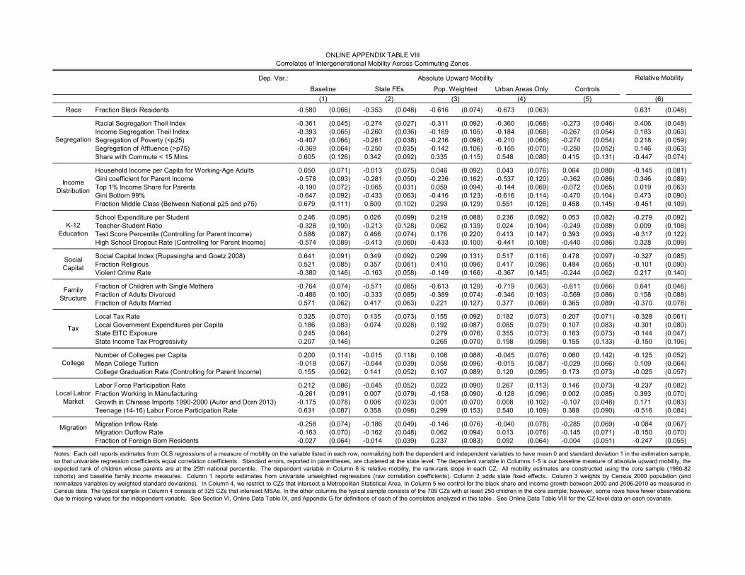
Dep. Var.:

Race Fraction Black Residents -0.580 (0.066) -0.353 (0.048) -0.616 (0.074) -0.673 (0.063) 0.631 (0.048)

Racial Segregation Theil Index -0.361 (0.045) -0.274 (0.027) -0.311 (0.092) -0.360 (0.068) -0.273 (0.046) 0.406 (0.048)Income Segregation Theil Index -0.393 (0.065) -0.260 (0.036) -0.169 (0.105) -0.184 (0.068) -0.267 (0.054) 0.183 (0.063)Segregation of Poverty (<p25) -0.407 (0.066) -0.261 (0.038) -0.216 (0.098) -0.210 (0.066) -0.274 (0.054) 0.218 (0.059)Segregation of Affluence (>p75) -0.369 (0.064) -0.250 (0.035) -0.142 (0.106) -0.155 (0.070) -0.250 (0.052) 0.146 (0.063)Share with Commute < 15 Mins 0.605 (0.126) 0.342 (0.092) 0.335 (0.115) 0.548 (0.080) 0.415 (0.131) -0.447 (0.074)

Household Income per Capita for Working-Age Adults 0.050 (0.071) -0.013 (0.075) 0.046 (0.092) 0.043 (0.076) 0.064 (0.080) -0.145 (0.081)Gini coefficient for Parent Income -0.578 (0.093) -0.281 (0.050) -0.236 (0.162) -0.537 (0.120) -0.362 (0.086) 0.346 (0.089)Top 1% Income Share for Parents -0.190 (0.072) -0.065 (0.031) 0.059 (0.094) -0.144 (0.069) -0.072 (0.065) 0.019 (0.063)Gini Bottom 99% -0.647 (0.092) -0.433 (0.063) -0.416 (0.123) -0.616 (0.114) -0.470 (0.104) 0.473 (0.090)Fraction Middle Class (Between National p25 and p75) 0.679 (0.111) 0.500 (0.102) 0.293 (0.129) 0.551 (0.126) 0.458 (0.145) -0.451 (0.109)

School Expenditure per Student 0.246 (0.095) 0.026 (0.099) 0.219 (0.088) 0.236 (0.092) 0.053 (0.082) -0.279 (0.092)Teacher-Student Ratio -0.328 (0.100) -0.213 (0.128) 0.062 (0.139) 0.024 (0.104) -0.249 (0.088) 0.009 (0.108)Test Score Percentile (Controlling for Parent Income) 0.588 (0.087) 0.466 (0.074) 0.176 (0.220) 0.413 (0.147) 0.393 (0.093) -0.317 (0.122)High School Dropout Rate (Controlling for Parent Income) -0.574 (0.089) -0.413 (0.060) -0.433 (0.100) -0.441 (0.108) -0.440 (0.086) 0.328 (0.099)

Social Capital Index (Rupasingha and Goetz 2008) 0.641 (0.091) 0.349 (0.092) 0.299 (0.131) 0.517 (0.116) 0.478 (0.097) -0.327 (0.085)Fraction Religious 0.521 (0.085) 0.357 (0.061) 0.410 (0.096) 0.417 (0.096) 0.484 (0.065) -0.101 (0.090)Violent Crime Rate -0.380 (0.146) -0.163 (0.058) -0.149 (0.166) -0.367 (0.145) -0.244 (0.062) 0.217 (0.140)

Fraction of Children with Single Mothers -0.764 (0.074) -0.571 (0.085) -0.613 (0.129) -0.719 (0.063) -0.611 (0.066) 0.641 (0.046)Fraction of Adults Divorced -0.486 (0.100) -0.333 (0.085) -0.389 (0.074) -0.346 (0.103) -0.569 (0.086) 0.158 (0.088)Fraction of Adults Married 0.571 (0.062) 0.417 (0.063) 0.221 (0.127) 0.377 (0.069) 0.365 (0.089) -0.370 (0.078)

Local Tax Rate 0.325 (0.070) 0.135 (0.073) 0.155 (0.092) 0.182 (0.073) 0.207 (0.071) -0.328 (0.061)Local Government Expenditures per Capita 0.186 (0.083) 0.074 (0.028) 0.192 (0.087) 0.085 (0.079) 0.107 (0.083) -0.301 (0.080)State EITC Exposure 0.245 (0.064) 0.279 (0.076) 0.355 (0.073) 0.163 (0.073) -0.144 (0.047)State Income Tax Progressivity 0.207 (0.146) 0.265 (0.070) 0.198 (0.098) 0.155 (0.133) -0.150 (0.106)

Number of Colleges per Capita 0.200 (0.114) -0.015 (0.118) 0.108 (0.088) -0.045 (0.076) 0.060 (0.142) -0.125 (0.052)Mean College Tuition -0.018 (0.067) -0.044 (0.039) 0.058 (0.096) -0.015 (0.087) -0.029 (0.066) 0.109 (0.064)College Graduation Rate (Controlling for Parent Income) 0.155 (0.062) 0.141 (0.052) 0.107 (0.089) 0.120 (0.095) 0.173 (0.073) -0.025 (0.057)

Labor Force Participation Rate 0.212 (0.086) -0.045 (0.052) 0.022 (0.090) 0.267 (0.113) 0.146 (0.073) -0.237 (0.082)Fraction Working in Manufacturing -0.261 (0.091) 0.007 (0.079) -0.158 (0.090) -0.128 (0.096) 0.002 (0.085) 0.393 (0.070)Growth in Chinese Imports 1990-2000 (Autor and Dorn 2013) -0.175 (0.078) 0.006 (0.023) 0.001 (0.070) 0.008 (0.102) -0.107 (0.048) 0.171 (0.083)Teenage (14-16) Labor Force Participation Rate 0.631 (0.087) 0.358 (0.098) 0.299 (0.153) 0.540 (0.109) 0.388 (0.090) -0.516 (0.084)

Migration Inflow Rate -0.258 (0.074) -0.186 (0.049) -0.146 (0.076) -0.040 (0.078) -0.285 (0.069) -0.084 (0.067)Migration Outflow Rate -0.163 (0.070) -0.162 (0.048) 0.062 (0.094) 0.013 (0.076) -0.145 (0.071) -0.150 (0.070)Fraction of Foreign Born Residents -0.027 (0.064) -0.014 (0.039) 0.237 (0.083) 0.092 (0.064) -0.004 (0.051) -0.247 (0.055)

Correlates of Intergenerational Mobility Across Commuting ZonesONLINE APPENDIX TABLE VIII

Notes: Each cell reports estimates from OLS regressions of a measure of mobility on the variable listed in each row, normalizing both the dependent and independent variables to have mean 0 and standard deviation 1 in the estimation sample,so that univariate regression coefficients equal correlation coefficients. Standard errors, reported in parentheses, are clustered at the state level. The dependent variable in Columns 1-5 is our baseline measure of absolute upward mobility, theexpected rank of children whose parents are at the 25th national percentile. The dependent variable in Column 6 is relative mobility, the rank-rank slope in each CZ. All mobility estimates are constructed using the core sample (1980-82cohorts) and baseline family income measures. Column 1 reports estimates from univariate unweighted regressions (raw correlation coefficients). Column 2 adds state fixed effects. Column 3 weights by Census 2000 population (andnormalizes variables by weighted standard deviations). In Column 4, we restrict to CZs that intersect a Metropolitan Statistical Area. In Column 5 we control for the black share and income growth between 2000 and 2006-2010 as measured inCensus data. The typical sample in Column 4 consists of 325 CZs that intersect MSAs. In the other columns the typical sample consists of the 709 CZs with at least 250 children in the core sample; however, some rows have fewer observationsdue to missing values for the independent variable. See Section VI, Online Data Table IX, and Appendix G for definitions of each of the correlates analyzed in this table. See Online Data Table VIII for the CZ-level data on each covariate.

Income Distribution

Tax

K-12 Education

Local Labor Market

Migration

Social Capital

Family Structure

Absolute Upward MobilityControls

(1) (4)Urban Areas Only

Relative Mobility

(6)(5)

College

Baseline State FEs Pop. Weighted(2) (3)

Segregation

FIGURE I: Association between Children’s and Parents’ Incomes

A. Level of Child Family Income vs. Parent Family Income

020

4060

8010

0

0 100 200 300 400

Mea

n C

hild

Hou

seho

ld In

com

e ($

1000

s)

Parent Household Income ($1000s)

Slope [Par Inc < P90] = 0.335

Slope [P90 < Par Inc < P99] = 0.076(0.0007)

(0.0019)

B. Log Child Family Income vs. Log Parent Family Income

0%5%

10%

15%

20%

Per

cent

age

of C

hild

ren

with

Zer

o In

com

e

9.5

1010

.511

8 10 12 14

Log Parent Income

Mean Log Child Inc. Frac. Children with Zero Inc.

Mea

n Lo

g C

hild

Inco

me

IGE = 0.344(0.0004)

(0.0007)IGE [Par Inc P10-P90] = 0.452

Notes: These figures present non-parametric binned scatter plots of the relationship between child income and parent income.Both figures are based on the core sample (1980-82 birth cohorts) and baseline family income definitions for parents andchildren. Child income is the mean of 2011-2012 family income (when the child is approximately 30 years old), while parentincome is mean family income from 1996-2000. Incomes are in 2012 dollars. To construct Panel A, we bin parent family incomeinto 100 equal-sized (centile) bins and plot the mean level of child income vs. mean level of parent income within each bin. Forscaling purposes, we do not show the point for the top 1% in Panel A. In the top 1% bin, mean parent income is $1.4 millionand mean child income is $114,000. In Panel B, we again bin parent family income into 100 bins and plot mean log income forchildren (left y-axis) and the fraction of children with zero family income (right y-axis) vs. mean parents’ log income. Childrenwith zero family income are excluded from the log income series. In both panels, the 10th and 90th percentile of parents’income are depicted in dashed vertical lines. The coefficient estimates and standard errors (in parentheses) reported on thefigures are obtained from OLS regressions on the microdata. In Panel A, we report separate slopes for parents below the 90thpercentile and parents between the 90th and 99th percentile. In panel B, we report slopes of the log-log regression (i.e., theintergenerational elasticity of income or IGE) in the full sample and for parents between the 10th and 90th percentiles.

FIGURE II: Association between Children’s and Parents’ Percentile Ranks

A. Mean Child Income Rank vs. Parent Income Rank in the U.S.

2030

4050

6070

Mea

n C

hild

Inco

me

Ran

k

0 10 20 30 40 50 60 70 80 90 100

Parent Income Rank

Rank-Rank Slope = 0.341(0.0003)

B. Cross-Country Comparisons

2030

4050

6070

0 10 20 30 40 50 60 70 80 90 100

Mea

n C

hild

Inco

me

Ran

k

Parent Income Rank CanadaDenmark

Rank-Rank Slope (Canada) = 0.174(0.005)

Rank-Rank Slope (Denmark) = 0.180(0.006)

United States

Notes: These figures present non-parametric binned scatter plots of the relationship between children’s and parent’s percentileincome ranks. Both figures are based on the core sample (1980-82 birth cohorts) and baseline family income definitions forparents and children. Child income is the mean of 2011-2012 family income (when the child is approximately 30 years old),while parent income is mean family income from 1996-2000. Children are ranked relative to other children in their birthcohort, while parents are ranked relative to all other parents in the core sample. Panel A plots the mean child percentile rankwithin each parent percentile rank bin. The series in triangles in Panel B plots the analogous series for Denmark, computedby Boserup, Kopczuk, and Kreiner (2013) using a similar sample and income definitions. The series in squares plots estimatesof the rank-rank series using the decile-decile transition matrix from Corak and Heisz (1999). The series in circles in PanelB reproduces the rank-rank relationship in the U.S. from Panel A as a reference. The slopes and best-fit lines are estimatedusing an OLS regression on the microdata for the U.S. and on the binned series (as we do not have access to the microdata)for Denmark and Canada. Standard errors are reported in parentheses.

FIGURE III: Robustness of Intergenerational Mobility Estimates

A. Lifecycle Bias: Rank-Rank Slopes by Age of Child

00.

10.

20.

30.

4

Ran

k-R

ank

Slo

pe

22 25 28 31 34 37 40

Population SOI 0.1% Random SampleAge at which Child’s Income is Measured

B. Attenuation Bias: Rank-Rank Slopes by Number of Years Used to Measure Parent Income

00.

10.

20.

30.

4

Ran

k-R

ank

Slo

pe

1 4 7 10 13 16

Years Used to Compute Mean Parent Income

Notes: This figure evaluates the robustness of the rank-rank slope estimated in Figure IIa to changes in the age at whichchild income is measured (Panel A) and the number of years used to measure parents’ income (Panel B). In both panels, childincome is defined as mean family income in 2011-2012. In Panel A, parent income is defined as mean family income from1996-2000. Each point in Panel A shows the slope coefficient from a separate OLS regression of child income rank on parentincome rank, varying the child’s birth cohort and hence the child’s age in 2011-12 when the child’s income is measured. Thecircles use the extended sample in the population data, while the triangles use the 0.1% Statistics of Income stratified randomsample. The first point in Panel A corresponds to the children in the 1990 birth cohort, who are 21-22 when their incomesare measured in 2011-12 (denoted by age 22 on the figure). The last point for which we have population-wide estimatescorresponds to the 1980 cohort, who are 31-32 (denoted by 32) when their incomes are measured. The last point in the SOIsample corresponds to the 1971 cohort, who are 40-41 (denoted by 41) when their incomes are measured. The dashed lineis a lowess curve fit through the SOI 0.1% sample rank-rank slope estimates. In Panel B, we focus on children in the coresample (1980-82 birth cohorts) in the population data. Each point in this figure shows the coefficient from the same rank-rankregression as in Figure IIa, varying the number of years used to compute mean parent income. The first point uses parentincome data for 1996 only to define parent ranks. The second point uses mean parent income from 1996-1997. The last pointuses mean parent income from 1996-2012, a 17 year average.

FIGURE IV: Gradients of College Attendance and Teenage Birth by Parent Rank

A. Children’s College Attendance Rate and Quality vs. Parent Income Rank

Coll. Quality Gradient (P75-P25) = 0.191

2040

6080

100

2040

6080

100

0 10 20 30 40 50 60 70 80 90 100

Coll. Attendance Slope = 0.675(0.0005)

Per

cent

Atte

ndin

g C

olle

ge a

t Age

s 18

-21

Col

lege

Qua

lity

Ran

k at

Age

20

Parent Income Rank College Attendance Rate College Quality Rank

(0.0010)

B. Female Children’s Teenage Birth Rate vs. Parent Income Rank

010

2030

Teen

age

Birt

h R

ate

(%)

0 10 20 30 40 50 60 70 80 90 100

Parent Income Rank

Slope = -0.298(0.0006)

Notes: These figures present non-parametric binned scatter plots of the relationship between children’s college attendancerates (Panel A, circles), college quality rank (Panel A, triangles), and teenage birth rates (Panel B) vs. parents’ percentilerank. Both figures are based on the core sample (1980-82 birth cohorts). Parent rank is defined based on mean family incomefrom 1996-2000. In Panel A, the circles plot the fraction of children ever attending college between age 18-21 within eachparent-income percentile bin; the triangles plot the average college quality rank at age 20 within each parent-income percentilebin. College attendance is defined as the presence of a 1098-T form filed by a college on behalf of the student. College qualityrank is defined as the percentile rank of the college that the child attends at age 20 based on the mean earnings at age 31 ofchildren who attended the same college (children who do not attend college are included in a separate “no college” group);see Section III.B for further details. Panel B plots the fraction of female children who give birth while teenagers within eachparental percentile bin. Having a teenage birth is defined as ever claiming a dependent child who was born while the motherwas aged 13-19. The slopes and best-fit lines for college attendance and teenage birth are estimated using linear regressionsof the outcome of interest on parent income rank in the microdata. We regress college quality rank on a quadratic in parentrank to match the non-linearity of the relationship. The college quality gradient is defined as the difference between the fittedvalues for children with parents at the 75th percentile and parents at the 25th percentile using this quadratic specification.

FIGURE V: Intergenerational Mobility in Selected Commuting Zones

A. Salt Lake City vs. Charlotte

2030

4050

6070

0 20 40 60 80 100

Mea

n C

hild

Ran

k in

Nat

iona

l Inc

ome

Dis

trib

utio

n

Parent Rank in National Income Distribution

Salt Lake City: ��� �

= 0.264, ��

= 46.2Charlotte:

��� �= 0.397,

��= 35.8

Salt Lake City Charlotte

B. San Francisco vs. Chicago

2030

4050

6070

0 20 40 60 80 100

Mea

n C

hild

Ran

k in

Nat

iona

l Inc

ome

Dis

trib

utio

n

Parent Rank in National Income Distribution

San Francisco: ��� �

= 0.250, ��

= 44.4Chicago:

��� �= 0.393,

��= 39.4

San Francisco Chicago

Notes: These figures present non-parametric binned scatter plots of the relationship between child and parent income ranksin selected CZs. Both figures are based on the core sample (1980-82 birth cohorts) and baseline family income definitions forparents and children. Children are assigned to commuting zones based on the location of their parents (when the child wasclaimed as a dependent), irrespective of where they live as adults. Parent and child percentile ranks are always defined atthe national level, not the CZ level. To construct each series, we group parents into 50 equally sized (two percentile point)bins and plot the mean child percentile rank vs. the mean parent percentile rank within each bin. We report two measuresof mobility based on the rank-rank relationships in each CZ. The first is relative mobility (r100 − r0), which is 100 times therank-rank slope estimate. The second is absolute upward mobility (r25), the predicted child income rank at the 25th percentileof parent income distribution, depicted by the dashed vertical line in the figures. All mobility statistics and best-fit lines areestimated on the underlying microdata (not the binned means).

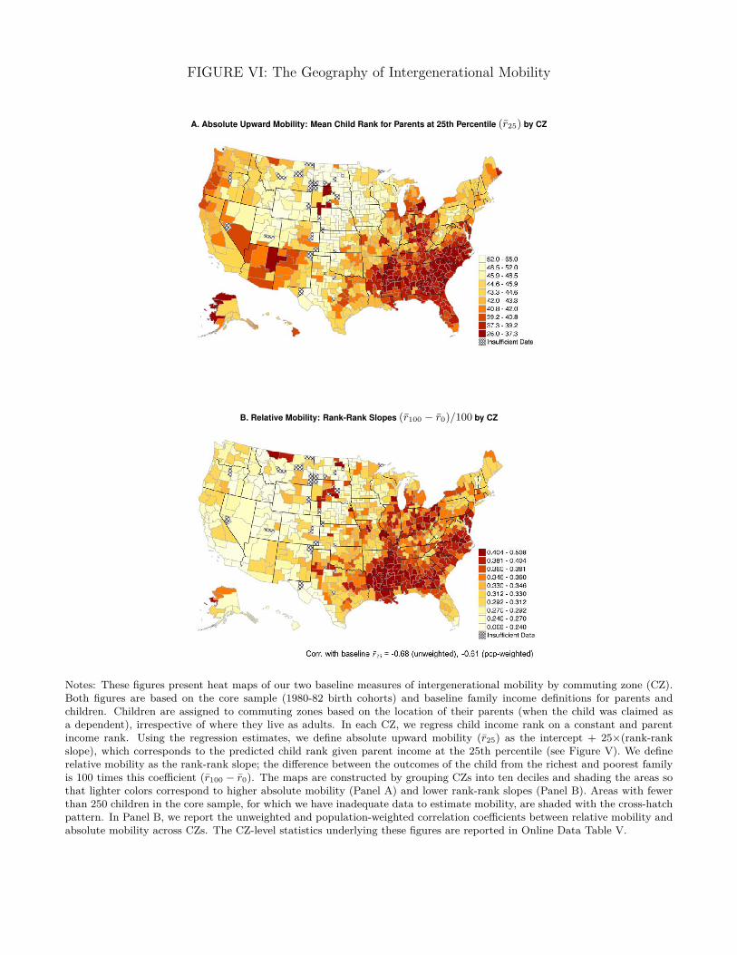
FIGURE VI: The Geography of Intergenerational Mobility

A. Absolute Upward Mobility: Mean Child Rank for Parents at 25th Percentile (r25) by CZ

B. Relative Mobility: Rank-Rank Slopes (r100 − r0)/100 by CZ

Notes: These figures present heat maps of our two baseline measures of intergenerational mobility by commuting zone (CZ).Both figures are based on the core sample (1980-82 birth cohorts) and baseline family income definitions for parents andchildren. Children are assigned to commuting zones based on the location of their parents (when the child was claimed asa dependent), irrespective of where they live as adults. In each CZ, we regress child income rank on a constant and parentincome rank. Using the regression estimates, we define absolute upward mobility (r25) as the intercept + 25×(rank-rankslope), which corresponds to the predicted child rank given parent income at the 25th percentile (see Figure V). We definerelative mobility as the rank-rank slope; the difference between the outcomes of the child from the richest and poorest familyis 100 times this coefficient (r100 − r0). The maps are constructed by grouping CZs into ten deciles and shading the areas sothat lighter colors correspond to higher absolute mobility (Panel A) and lower rank-rank slopes (Panel B). Areas with fewerthan 250 children in the core sample, for which we have inadequate data to estimate mobility, are shaded with the cross-hatchpattern. In Panel B, we report the unweighted and population-weighted correlation coefficients between relative mobility andabsolute mobility across CZs. The CZ-level statistics underlying these figures are reported in Online Data Table V.

FIGURE VII: Relationship Between Absolute and Relative Mobility

A. Association Between Absolute and Relative Mobility by Parent Income Rank

-1.0

-0.5

00.

5

0 20 40 60 80 100

Mean Pivot Point = 85.1th Percentile

Parent Rank in National Income Distribution

Coe

f. fr

om R

egre

ssio

n of

Chi

ld R

ank

on R

elat

ive

Mob

ility

B. Illustrative Schematic of Pivot in Rank-Rank Relationship

2030

4050

6070

0 20 40 60 80 100

Average Pivot Point: = 85.1

Parent Rank in National Income Distribution

Chi

ld R

ank

in N

atio

nal I

ncom

e D

istr

ibut

ion

Low Rank-Rank Slope

High Rank-Rank Slope

Notes: These figures illustrate the correlation between relative mobility and absolute mobility at various percentiles of theincome distribution. To construct Panel A, we first calculate the mean income rank of children in CZ c with parents in(national) percentile p, denoted by µpc. We then run a CZ-level regression of µpc on relative mobility (r100c − r0c) at eachpercentile p separately. Panel A plots the resulting regression coefficients γp vs. the percentile p. The coefficient γp can beinterpreted as the mean impact of a 1 unit increase in relative mobility on the absolute outcomes of children whose parents areat percentile p. We also plot the best linear fit across the 100 coefficients. This line, estimated using an OLS regression, crosseszero at percentile p = 85.1. This implies that increases in relative mobility are associated with higher expected rank outcomesfor children with parents below percentile 85.1 and lower expected rank outcomes for children with parents above percentile85.1. To illustrate the intuition for this result, Panel B plots hypothetical rank-rank relationships in two representative CZs,one of which has more relative mobility than the other. Panel A implies that in such a pairwise comparison, the two rank-rankrelationships cross at the 85th percentile on average, as illustrated in Panel B.

FIGURE VIII: Correlates of Spatial Variation in Upward Mobility

Frac. Foreign Born (-)Migration Outflow (-)

Migration Inflow (-)

Teenage LFP Rate (+)Chinese Import Growth (-)

Manufacturing Share (-)

Coll Grad Rate (Inc Adjusted) (+)College Tuition (-)

Colleges per Capita (+)

Tax Progressivity (+)State EITC Exposure (+)

Local Tax Rate (+)

Frac. Married (+)Divorce Rate (-)

Frac. Single Moms (-)

Violent Crime Rate (-)Frac. Religious (+)

Social Capital Index (+)

High School Dropout (-)Test Scores (Inc Adjusted) (+)

Student-Teacher Ratio (-)

Top 1% Inc. Share (-)Gini Coef. (-)

Mean Household Income (+)

Frac. < 15 Mins to Work (+)Segregation of Poverty (-)

Racial Segregation (-)

Frac. Black Residents (-)

0 0.2 0.4 0.6 0.8 1.0

Correlation

TAX

MIG

SE

GK

-12

G INC

LAB

FAM

SO

CC

OLL

Notes: This figure shows the correlation of various CZ-level characteristics with absolute upward mobility (r25) across CZs.For each characteristic listed on the y axis, the dot represents the absolute value of the unweighted correlation of the variablewith r25 across CZs. The horizontal bars show the 95% confidence interval based on standard errors clustered at state level.Positive correlations are shown by (+) on the y axis; negative correlations are shown by (-). We consider covariates in tenbroad categories: racial demographics, segregation, properties of the income distribution, K-12 education, social capital, familystructure, local tax policies, college education, labor market conditions, and migration rates. The categories with the highestcorrelations are highlighted. See Column 1 of Appendix Table VII for the point estimates corresponding to the correlationsplotted here. See Section VI, Online Data Table IX, and Online Appendix G for definitions of each of the correlates. CZ-leveldata on the covariates used in this figure are reported in Online Data Table VIII.

FIGURE IX: Race and Upward Mobility

A. Upward Mobility for Individuals in 80%+ White ZIP Codes

B. Impact of Changing Racial Composition of Sample on CZ-Level Estimates of Upward Mobility

0.2

.4.6

.81

0.70 0.75 0.80 0.85 0.90 0.95 1.00

Fraction of White Individuals in Restricted Sample

Empirical EstimatesPrediction with No SpatialHeterogeneity Cond. on Race

Coe

f. fr

om R

egre

ssio

n of

on

Notes: Panel A presents a heat map of absolute upward mobility for individuals living in ZIP codes with 80% or more whiteresidents. This figure replicates Figure VIa, restricting the sample used to estimate the rank-rank regression in each CZ toparents living in ZIP codes with 80% or more white residents. Note that we color the entire CZ based on the resulting estimateof upward mobility (not just the ZIP codes used in the estimation) for comparability to other figures. CZs with fewer than250 children living in ZIP codes with >80% white share are omitted and shaded with the cross-hatch pattern. We report theunweighted and population-weighted correlation coefficients between this measure and absolute upward mobility presentedin Figure VIa across CZs. To construct Panel B, we first compute upward mobility in each CZ, restricting the sample toindividuals living in ZIP codes that are more than w% white, which we denote by rw

25,c. We then regress rw25,c on r25,c, our

baseline estimates of upward mobility based on the full sample, using an unweighted OLS regression with one observationper CZ with available data. We vary w from 0% to 95% in increments of 5% and plot the resulting regression coefficientsagainst the fraction of white individuals in each of the subsamples. The confidence interval, shown by the dotted lines aroundthe point estimates, is based on standard errors clustered at the state level. The dashed diagonal line shows the predictedrelationship if there were no spatial heterogeneity in upward mobility conditional on race.

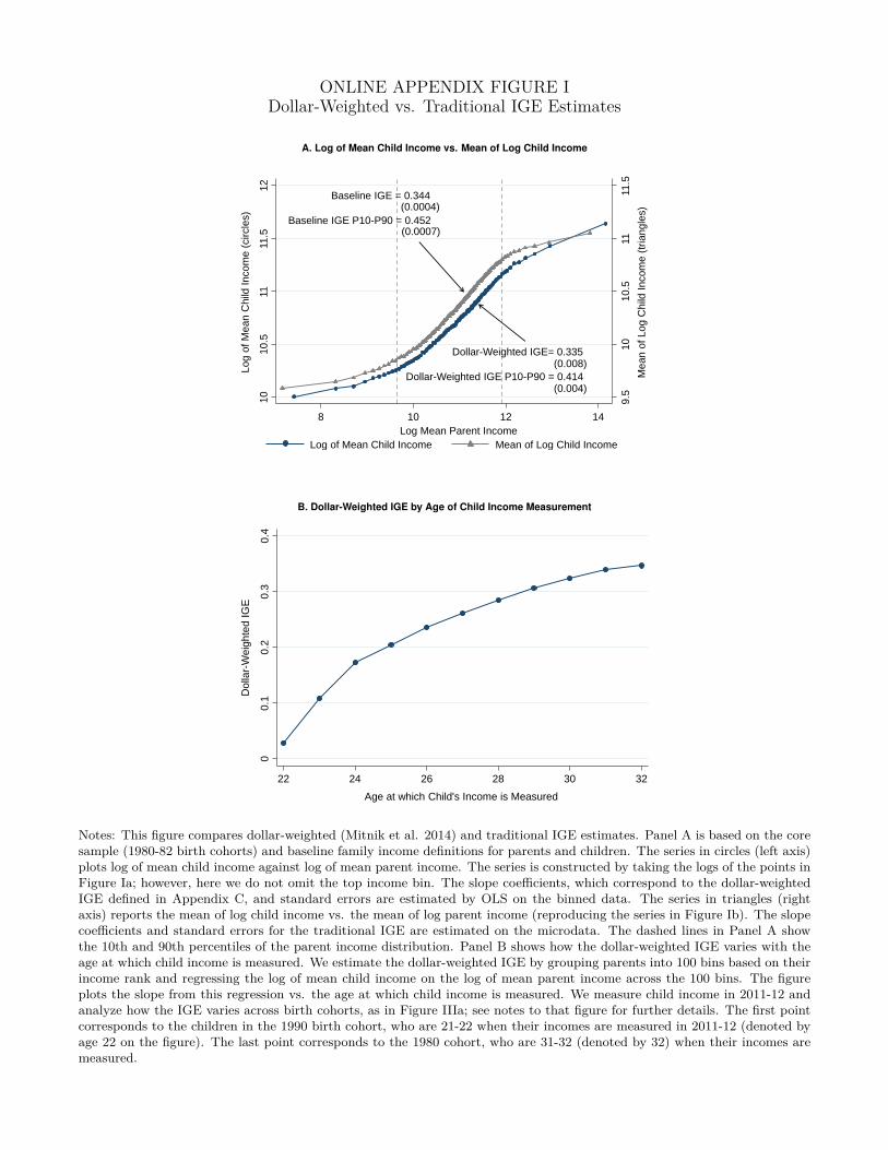
ONLINE APPENDIX FIGURE IDollar-Weighted vs. Traditional IGE Estimates

A. Log of Mean Child Income vs. Mean of Log Child Income

9.5

1010

.511

11.5

Mea

n of

Log

Chi

ld In

com

e (t

riang

les)

1010

.511

11.5

12

Log

of M

ean

Chi

ld In

com

e (c

ircle

s)

8 10 12 14Log Mean Parent Income

Log of Mean Child Income Mean of Log Child Income

Baseline IGE = 0.344(0.0004)

Baseline IGE P10-P90 = 0.452(0.0007)

Dollar-Weighted IGE= 0.335(0.008)

(0.004)Dollar-Weighted IGE P10-P90 = 0.414

B. Dollar-Weighted IGE by Age of Child Income Measurement

00.

10.

20.

30.

4

Dol

lar-

Wei

ghte

d IG

E

22 24 26 28 30 32

Age at which Child's Income is Measured

Notes: This figure compares dollar-weighted (Mitnik et al. 2014) and traditional IGE estimates. Panel A is based on the coresample (1980-82 birth cohorts) and baseline family income definitions for parents and children. The series in circles (left axis)plots log of mean child income against log of mean parent income. The series is constructed by taking the logs of the points inFigure Ia; however, here we do not omit the top income bin. The slope coefficients, which correspond to the dollar-weightedIGE defined in Appendix C, and standard errors are estimated by OLS on the binned data. The series in triangles (rightaxis) reports the mean of log child income vs. the mean of log parent income (reproducing the series in Figure Ib). The slopecoefficients and standard errors for the traditional IGE are estimated on the microdata. The dashed lines in Panel A showthe 10th and 90th percentiles of the parent income distribution. Panel B shows how the dollar-weighted IGE varies with theage at which child income is measured. We estimate the dollar-weighted IGE by grouping parents into 100 bins based on theirincome rank and regressing the log of mean child income on the log of mean parent income across the 100 bins. The figureplots the slope from this regression vs. the age at which child income is measured. We measure child income in 2011-12 andanalyze how the IGE varies across birth cohorts, as in Figure IIIa; see notes to that figure for further details. The first pointcorresponds to the children in the 1990 birth cohort, who are 21-22 when their incomes are measured in 2011-12 (denoted byage 22 on the figure). The last point corresponds to the 1980 cohort, who are 31-32 (denoted by 32) when their incomes aremeasured.

ONLINE APPENDIX FIGURE IIAdditional Evidence on Robustness of Intergenerational Mobility Estimates

A. IGE Estimates by Age of Child Income Measurement

00.

20.

40.

6

Ran

k-R

ank

Slo

pe

22 25 28 31 34 37 40

Population SOI 0.1% Random SampleAge at which Child’s Income is Measured

B. Rank-Rank Slope by Age of Parent Income Measurement

Ran

k-R

ank

Slo

pe

41 43 45 47 49 51 53 55

Mother’s Age when Parent Income Measured

00.

10.

20.

30.

4

C. College Attendance Gradient by Age of ChildWhen Parent Income is Measured

00.

20.

40.

60.

8

Col

lege

Atte

ndan

ce G

radi

ent

3 6 9 12 15 18

Age of Child when Parent Income is Measured

D. Rank-Rank Slope by Number of YearsUsed to Measure Child Income

00.

10.

20.

30.

4

Ran

k-R

ank

Slo

pe

1 2 3 4 5 6

Years used to Compute Mean Child Income

Notes: This figure evaluates the robustness of intergenerational mobility measures to lifecycle and attenuation bias. Panel Aevaluates the robustness of the IGE to changes in the age at which child income is measured. Panel B evaluates the robustnessof the rank-rank slope to changes in the age at which parent income is measured. Panel C evaluates the robustness of thecollege attendance gradient to the age of the child when parent income is measured. Panel D evaluates the robustness ofthe rank-rank slope to the number of years used to measure the child’s income. In Panel A, we estimate the log-log IGE(excluding children with zero income), varying the age at which child income is measured. We restrict the sample to parentswith income between the 10th and 90th percentile when estimating the IGE, as shown in Figure Ib. We measure child incomein 2011-12 and analyze how the IGE varies across birth cohorts, as in Figure IIIa; see notes to that figure for further details.In Panel B, each point shows the slope coefficient from an OLS regression of child income rank on parent income rank (as inFigure IIa), using the core sample and varying the age at which parent income rank is measured. The first point measuresparent income in 1996, when the mean age of mothers is 41. The last point measures income in 2010, when parents are 55.Panel C reproduces Appendix Figure 2b from Chetty et al. (2014). In this figure, each point shows the slope coefficient froman OLS regression of an indicator for the child attending college at age 19 on parent income rank (similar to Figure IVa),varying the year in which parent income rank is measured from 1996 to 2011. In this series, we use data from the 1993 birthcohort, which allows us to analyze parent income starting when children are 3 years old in 1996. We list the age of the childon the x axis to evaluate whether the gradient differs when children are young (although parent age is of course also rising inlockstep). In Panel D, each point shows the slope coefficient from the same rank-rank regression as in Panel B using the coresample, but here we always use a five-year (1996-2000) mean to measure parent income and vary the number of years used tocompute mean child income. The point for one year measures child income in 2012 only. The point for two years uses meanchild income in 2011-12. We continue adding data for prior years; the 6th point uses mean income in years 2007-2012.

ONLINE APPENDIX FIGURE IIIBoston Commuting Zone

BostonWorcester

Middlesex

Essex

Norfolk

Plymouth

Barnstable

Suffolk

Notes: This figure shows a map of the counties that comprise the Boston Commuting Zone. The city of Boston is shown bythe arrow.

ONLINE APPENDIX FIGURE IVRank-Rank Relationships and Income Distributions in the 20 Largest CZs

.51

1.5

22.

5.5

11.

52

2.5

.51

1.5

22.

5.5

11.

52

2.5

.2.4

.6.8

.2.4

.6.8

.2.4

.6.8

.2.4

.6.8

0 50 100 0 50 100 0 50 100 0 50 100 0 50 100

Atlanta, GA Boston, MA Bridgeport, CT Chicago, IL Cleveland, OH

Dallas, TX Detroit, MI Houston, TX Los Angeles, CA Miami, FL

Minneapolis, IN New York, NY Newark, NJ Philadelphia, PA Phoenix, AZ

Sacramento, CA San Diego, CA San Francisco, CA Seattle, WA Washington DC

Rel

ativ

e D

ensi

ty o

f Par

ent I

ncom

e D

istr

ibut

ion

Mea

n C

hild

Ran

k in

Nat

iona

l Dis

trib

utio

n

Parents' Percentile Rank in National Income Distribution

Notes: These figures present non-parametric binned scatter plots (shown by the points and solid line, left y-axis) of therelationship between child and parent income ranks in the twenty largest CZs based on population in the 2000 Census. Allfigures are based on the core sample (1980-82 birth cohorts) and baseline family income definitions for parents and children.Children are assigned to commuting zones based on the location of their parents. Parent and child percentile ranks are alwaysdefined at the national level, not the CZ level. To construct each rank-rank series, we group parents into 50 equally sized(two percentile point) bins and plot the mean child percentile rank vs. the mean parent percentile rank within each bin. Thedashed curve (right y-axis) in each panel depicts the income distribution in the CZ relative to the national distribution. Thiscurve plots the share of parents with income in each bin in the CZ divided by the share in the same bin in the national incomedistribution. By construction, this curve averages to one in each CZ, shown by the horizontal dashed line in each panel.

ONLINE APPENDIX FIGURE VEstimates of Absolute Upward Mobility Pooling 1980-82 and 1980-85 Cohorts

Notes: The figure presents the map of absolute upward mobility by CZ shown on the project homepage (www.equality-of-opportunity.org). For the 709 CZs that have at least 250 children in the 1980-82 cohorts, we compute absolute upward mobilityexactly as in Figure VIa. For an additional 22 CZs that have fewer than 250 children in the 1980-82 cohorts but at least250 children in the 1980-85 cohorts, we report estimates of absolute upward mobility using the 1980-85 birth cohorts. Weestimate absolute upward mobility using exactly the same procedure as described in the notes to Figure VIa. The map isconstructed by grouping CZs into ten deciles based on the hybrid absolute mobility measure and shading the areas so thatlighter colors correspond to higher absolute mobility. Areas with fewer that 250 children in the 1980-85 cohorts are shadedwith the cross-hatch pattern.The CZ-level statistics underlying this map are reported in Online Data Table V.

ONLINE APPENDIX FIGURE VIAlternative Measures of Upward Mobility

A. Absolute Upward Mobility Adjusted for Local Cost-of-Living B. Probability of Reaching Top Quintile from Bottom Quintile

C. Fraction of Children Above Poverty Line Given Parents at 25th Percentile

Notes: These figures present heat maps for alternative measures of upward income mobility. Children are assigned to commut-ing zones based on the location of their parents (when the child was claimed as a dependent), irrespective of where they liveas adults. All panels use baseline family income definitions for parents. Panels A and C use the core sample (1980-82 birthcohorts) and panel B uses the 1980-85 birth cohorts. Panel A replicates Figure VIa, adjusting for differences in cost-of-livingacross areas. To construct this figure, we first deflate parent income by a cost-of-living index (COLI) for the parent’s CZ whenhe/she claims the child as a dependent and child income by a COLI for the child’s CZ in 2012. We then compute parentand child ranks using the resulting real income measures and replicate the procedure in Figure VIa exactly. The COLI isconstructed using data from the ACCRA price index combined with information on housing values and other variables asdescribed in Appendix A. Panel B presents a heat map of the probability that a child reaches the top quintile of the nationalfamily income distribution for children conditional on having parents in the bottom quintile of the family income distributionfor parents. These probabilities are taken directly from Online Data Table VI. Panel C shows the fitted values at parentrank 25 from a regression of an indicator for child family income being above the poverty line on parent income rank (seeAppendix F for details). The maps are constructed by grouping CZs into ten deciles and shading the areas so that lighter colorscorrespond to higher mobility. Areas with fewer that 250 children in the core sample (or the 1980-85 cohorts for Panel B), forwhich we have inadequate data to estimate mobility, are shaded with the cross-hatch pattern. We report the unweighted andpopulation-weighted correlation coefficient across CZs between these mobility measures and the baseline measure in FigureVIa. The CZ-level statistics underlying Panels A and C are reported in Online Data Table V.

ONLINE APPENDIX FIGURE VIIThe Geography of College Attendance by Parent Income Gradients

A. Slope of College Attendance-Parent Rank Gradients by CZ

B. College Attendance Rates for Children with Parents at the 25th Percentile by CZ

Notes: To construct these figures, we regress an indicator for college attendance on parent income rank (in the nationaldistribution) for each CZ separately. College attendance is defined by the presence of a 1098-T form filed by a college onbehalf of the student. We use the core sample (1980-82 birth cohorts) and baseline family income definitions for parents.Children are assigned to commuting zones based on the location of their parents (when the child was claimed as a dependent),irrespective of where they live as adults. In Panel A, we map the slope coefficients on the college attendance indicator fromthe CZ-level regressions. Panel B maps the fitted values from the regressions at parent rank 25. The maps are constructedby grouping CZs into ten deciles and shading the areas so that lighter colors correspond to higher mobility (smaller slopesin Panel A and higher fitted values in Panel B). Areas with fewer that 250 children in the core sample, for which we haveinadequate data to estimate mobility, are shaded with the cross-hatch pattern. We report the unweighted and population-weighted correlation coefficients across CZs between these mobility measures and the baseline measures in Figure VI. TheCZ-level statistics underlying these figures are reported in Online Data Table V.

ONLINE APPENDIX FIGURE VIIIThe Geography of College Quality by Parent Income Gradients

A. College Quality Gradient (P75-P25) by CZ

B. Mean College Quality Rank for Children with Parents at the 25th Percentile by CZ

Notes: To construct these figures, we regress college quality rank on a quadratic in parent income rank (in the nationaldistribution) for each CZ separately. College quality rank is defined as the percentile rank of the college that the child attendsat age 20 based on the mean earnings at age 31 of children who attended the same college (children who do not attend collegeare included in a separate “no college” group); see Section III.B for further details. We use the core sample (1980-82 birthcohorts) and baseline family income definitions for parents. Children are assigned to commuting zones based on the locationof their parents (when the child was claimed as a dependent), irrespective of where they live as adults. In Panel A, we mapthe college quality income gradient, defined as the difference between the fitted values at parent rank 75 and parent rank 25from the CZ-level regressions. Panel B maps the fitted values of college quality rank at parent rank 25 from these regressions.The maps are constructed by grouping CZs into ten deciles and shading the areas so that lighter colors correspond to highermobility (smaller gradients in Panel A and higher fitted values in Panel B). Areas with fewer that 250 children in the coresample, for which we have inadequate data to estimate mobility, are shaded with the cross-hatch pattern. We report theunweighted and population-weighted correlation coefficients across CZs between these mobility measures and the baselinemeasures in Figure VI. The CZ-level statistics underlying these figures are reported in Online Data Table V.

ONLINE APPENDIX FIGURE IXThe Geography of Teenage Birth by Parent Income Gradients

A. Slope of Teenage Birth-Parent Rank Gradients by CZ

B. Teenage Birth Rates for Children with Parents at the 25th Percentile by CZ

Notes: To construct these figures, we regress an indicator for teenage birth on parent income rank (in the national distribution)for each CZ separately. Teenage birth is defined as ever claiming a dependent child who was born while the mother was aged13-19. We use female children in the core sample (1980-82 birth cohorts) and baseline family income definitions for parents.Children are assigned to commuting zones based on the location of their parents (when the child was claimed as a dependent),irrespective of where they live as adults. In Panel A, we map the slope coefficient on the teenage birth indicator from the CZ-level regressions. Panel B maps the fitted values from these regressions at parent income rank 25. The maps are constructedby grouping CZs into ten deciles and shading the areas so that lighter colors correspond to smaller slopes (in magnitudes)in Panel A and smaller fitted values in Panel B. Areas with fewer that 250 female children in the core sample, for which wehave inadequate data to estimate mobility measures, are shaded with the cross-hatch pattern. We report the unweighted andpopulation-weighted correlation coefficients across CZs between these mobility measures and the baseline measures in FigureVI. The CZ-level statistics underlying these figures are reported in Online Data Table V.

ONLINE APPENDIX FIGURE XSegregation and Upward Mobility

A. Upward Mobility vs. Theil Index of Racial Segregation in CZ

3540

4550

55

0.01 0.02 0.05 0.14 0.37

Theil Index of Racial Segregation in 2000 (log scale)

Correlation = -0.361(0.045)

Upw

ard

Mob

ility

)

B. Upward Mobility vs. Rank-Order Index of Income Segregation in CZ

3540

4550

55

0.002 0.007 0.018 0.050 0.135

Rank-Order Index of Income Segregation (log scale)

Upw

ard

Mob

ility

��

)

Correlation = -0.393(0.065)

Notes: Panel A presents a binned scatter plot of absolute upward mobility (r25) vs. a multi-group Theil index of racialsegregation (based on census tract level data from the 2000 Census). To construct this figure, we group CZs into twentyequally sized bins (vingtiles) based on their segregation index. We then plot the mean level of absolute upward mobility vs.the mean segregation index within each of the twenty bins (using a log scale on the x axis). Panel B presents an analogousbinned scatter plot of absolute upward mobility vs. the rank-order index of income segregation from Reardon (2011). Seetext for details on the construction of these segregation indices. Note that these binned scatter plots provide a non-parametricrepresentation of the conditional expectation function, but they do not show the variance in the underlying data across CZs.The correlations between the variables are estimated using the underlying CZ-level data, with standard errors (reported inparentheses) clustered by state. The correlations are estimated in levels (not logs) for consistency with Appendix Table VII.

ONLINE APPENDIX FIGURE XILocal Income Distributions and Upward Mobility

A. Upward Mobility vs. Mean Income in CZ

3540

4550

55

22.0 26.9 32.9 40.1 49.0

Correlation = 0.050(0.071)

Mean Income per Working Age Adult ($1000s, log scale)

Upw

ard

Mob

ility

)

B. Upward Mobility vs. Gini Coefficient in CZThe “Great Gatsby” Curve Within the U.S.

3540

4550

55

0.3 0.4 0.5 0.6

Correlation = -0.578(0.093)

Upw

ard

Mob

ility

)

Gini Coef. for Parent Family Income (1996-2000)

C. Upward Mobility vs. Top 1% Income Share in CZ

3540

4550

55

0.05 0.08 0.14 0.22

Correlation = -0.190(0.072)

Top 1% Income Share Based on Parent Family Income (1996-2000, log scale)

Upw

ard

Mob

ility

)

Notes: Panel A presents a binned scatter plot of absolute upward mobility (r25) vs. mean income per working age adultin the CZ (based on data from the 2000 Census). To construct this figure, we group CZs into twenty equally sized bins(vingtiles) based on mean income levels. We then plot the mean level of absolute upward mobility vs. the mean incomelevel within each of the twenty bins (using a log scale on the x axis). Panel B presents an analogous binned scatter plot ofabsolute upward mobility vs. the Gini coefficient in the CZ, computed based on the core sample and mean parent income for1996-2000. Panel C presents a binned scatter plot of absolute upward mobility vs. the fraction of income in the CZ accruingto parents in the top 1% of the local distribution (using a log scale on the x axis), again using the core sample and parents’average income for 1996-2000. Note that these binned scatter plots provide a non-parametric representation of the conditionalexpectation function, but they do not show the variance in the underlying data across CZs. The correlations between thevariables are estimated using the underlying CZ-level data, with standard errors (reported in parentheses) clustered by state.The correlations are estimated in levels (not logs) for consistency with Appendix Table VII.

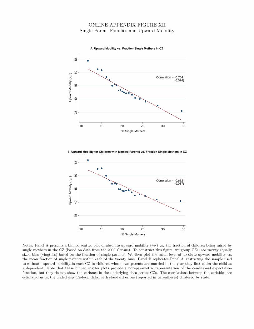
ONLINE APPENDIX FIGURE XIISingle-Parent Families and Upward Mobility

A. Upward Mobility vs. Fraction Single Mothers in CZ

3540

4550

55

10 15 20 25 30 35

% Single Mothers

Upw

ard

Mob

ility

��

)

Correlation = -0.764(0.074)

B. Upward Mobility for Children with Married Parents vs. Fraction Single Mothers in CZ

3540

4550

55

10 15 20 25 30 35

% Single Mothers

Upw

ard

Mob

ility

��

)

Correlation = -0.662(0.087)

Notes: Panel A presents a binned scatter plot of absolute upward mobility (r25) vs. the fraction of children being raised bysingle mothers in the CZ (based on data from the 2000 Census). To construct this figure, we group CZs into twenty equallysized bins (vingtiles) based on the fraction of single parents. We then plot the mean level of absolute upward mobility vs.the mean fraction of single parents within each of the twenty bins. Panel B replicates Panel A, restricting the sample usedto estimate upward mobility in each CZ to children whose own parents are married in the year they first claim the child asa dependent. Note that these binned scatter plots provide a non-parametric representation of the conditional expectationfunction, but they do not show the variance in the underlying data across CZs. The correlations between the variables areestimated using the underlying CZ-level data, with standard errors (reported in parentheses) clustered by state.

ONLINE APPENDIX FIGURE XIIIPredicted vs. Actual Time Trends in Relative Mobility

.2.2

5.3

.35

.4

1970 1980 1990

Ran

k-R

ank

Slo

pe

Birth Cohort

Rank-Rank Slope Coll. Forecast of R-R Slope Racial Seg.

Gini Bottom 99% Frac. Religious HS Dropout Frac. Single Mothers

Notes: This figure compares actual trends in rank-rank slopes at the national level, estimated in Chetty et al. (2014), withprojected changes based on trends in the five factors most strongly correlated with differences in mobility across CZs in thecross-section. The series in circles is from Chetty et al. (2014, Figure 2). The solid circles show estimates of rank-rankslopes by birth cohort using the SOI 0.1% sample. The open circles show forecasts of the rank-rank slope based on incomemeasured at age 26 and the college attendance rates using the population data. The other series show projections of trends,each based on a different factor: (1) Theil index of racial segregation, (2) high school dropout rate, (3) Gini coefficient, (4)violent crime arrest rate, and (5) fraction of single parents. We construct these projections based on unweighted univariateCZ-level regressions of relative mobility on each factor separately. We normalize the projections (by adding a constant) sothat their values match the mean observed rank-rank slope (i.e., the mean value of the series in circles) from 1971-1990. SeeAppendix I for further details.