“TIM Working Paper Series”

Vol. 2 – 2009

WPS 2#2

A GUIDELINE TO META-ANALYSIS

Alexander Kock

Lehrstuhl für Technologie- und Innovationsmanagement

Technische Universität Berlin

Prof. Dr. H. G. Gemünden

Straße des 17. Juni 135

10623 Berlin

alexander.kock@tim.tu-berlin.de

2

ABSTRACT

Scientific research is growing almost explosively as researchers in many

scientific fields are producing eminent numbers of empirical studies on the

relationship between variables of interest. This flood of information often makes

it impossible for scholars to have an overview of the development and the state

of findings that contribute to the overall picture of a research field.

Furthermore, findings are often contradictive and cause confusion among

researchers who seek to draw general conclusion from previous research. A

method for the quantitative synthesis of research findings is meta-analysis,

which applies statistical techniques to sum up the body of empirical data in a

research domain. The approach of meta-analysis has grown in popularity over

the past decades and is considered to be the wave of the future in handling

synthesis of research findings. This paper gives a detailed overview of Hunter

and Schmidt’s approach to meta-analysis of correlation coefficients. Basic

principles such as the underlying fixed- and random-effects models in meta-

analysis, along with criticism towards the validity of meta-analytic results, are

discussed. The core section of the paper outlines step-by-step instructions of the

statistical procedures involved in order to give researchers a guideline to

conduct meta-analyses.

1 Introduction

“Scientific research in nearly every field is growing almost explosively” (Rosenthal and

DiMatteo, 2001: 60). Scholars in research domains such as psychological, medical,

educational or management science generate abundant quantities of research findings, which

are often confusing and conflicting about central issues of theory and practice. As a result it is

virtually impossible for researchers to have an overview of all findings in a particular

research field. Methods that synthesize previous findings and give insights into the overall

picture of a particular research domain are required.

Synthesizing research findings across studies is often done in the form of a narrative

literature review that provides a qualitative and often subjective summary of previous

research (Mann, 1990: 476). Contrary to narrative reviews, meta-analysis takes a quantitative

approach because it makes use of statistical techniques in order to estimate a possible effect

between a dependent and an independent variable in a population (Song et al., 2001: 135). As

meta-analysis increases the sample size by aggregating study findings, it “allows researchers

to arrive at conclusions that are more accurate and more credible than can be presented in any

one primary study or in a non-quantitative, narrative review” (Rosenthal and DiMatteo, 2001:

3

61). Meta-analysis combines effect sizes from different studies to an overall measurement,

calls attention to the effect that is associated with the random sampling process in primary

studies, corrects individual study findings for study imperfections, and examines the

variability among previous study findings (Hunter and Schmidt, 2004: 33-56; Viechtbauer,

2007: 29). If this variability cannot be explained by artificial error alone, meta-analysis

furthermore aims for identification of moderating effects (Whitener, 1990). These moderators

may predict patterns among noticeable differences in research outcomes and therefore may

enlighten why study outcomes seem confusing and conflicting at first sight.

Despite these advantages, meta-analysis requires considerably more expertise and

knowledge in statistical methods and procedures than a narrative review (Lipsey and Wilson,

2001: 9). Field (2003: 111) argues that many researchers fail to distinguish between fixed-

and random-effects models in meta-analysis and predominantly apply fixed-effects models to

random-effects data, which can lead to false conclusions about statistical significance of

aggregated findings (Hedges and Vevea, 1998: 500). Even though Hunter and Schmidt (1990;

2004) have proposed a sophisticated meta-analytical method that enables the researcher to

correct research findings for study imperfections, “this unique focus … is seldom fully used”

(Johnson et al., 1995: 96). Hunter and Schmidt (2004: 80) report that most researchers

abandon study imperfections when doing meta-analysis. In those cases of conducting a “bare-

bones meta-analysis”, the estimation of the population effect size is biased and the bare-bones

variance is usually a very poor estimate of the real variance (Hunter and Schmidt, 2004: 132).

In light of these insights, the goal of this paper is to clarify the procedures and methods

applied in meta-analysis and to present an easy-to-follow guideline for their appropriate use.

The paper is organized as follows. First we will outline the concept and basic principles of

meta-analysis along with a discussion of the criticism towards meta-analysis. Then a detailed

guideline of statistical methods and calculations used in meta-analysis follows. Finally, we

discuss how moderator effects can be detected and evaluated.

2 Concept of Meta-Analysis

2.1 Development of Meta-Analysis

Gene V. Glass coined the term “Meta-Analysis” when he presented his method for

quantitative research synthesis at the conference of the American Educational Research

4

Association in 1976 (Hedges, 1992: 279; Johnson et al., 1995: 95; Franke, 2001: 186;

Rosenthal and DiMatteo, 2001: 62). Since then the popularity of meta-analysis has increased

significantly. A literature scan on the EBSCO database for articles that contain the term

“meta-analysis” in the title or the subject reveals a distinct publishing pattern.

Figure 1: Development of Meta-Analysis

Whereas the number of published articles in the 1980’s was persistently lower than 20

publications per year, meta-analysis related publications have increased over the 1990’s to

more than 200 per year and have since then grown to more than one thousand publications in

the year 2007 alone. Since books on meta-analytical methods became common in the early

1980s, three major meta-analytic approaches have remained popular (see Johnson et al.,

1995): the Hedges and Olkin (1985) technique, the Rosenthal and Rubin technique

(Rosenthal and Rubin, 1978; Rosenthal and Rubin, 1988; Rosenthal, 1991), and the Hunter

and Schmidt technique (Hunter et al., 1982; Hunter and Schmidt, 1990; Hunter and Schmidt,

2004).

The Hedges and Olkin technique usually converts individual study findings into standard

deviation units which are then corrected for bias, whereas the Rosenthal and Rubin technique

convert study outcomes to Fisher Z standard normal metrics before combining results across

studies. Johnson et al. (1995: 105) have shown that both techniques lead to very similar

5

results with respect to the statistics that each technique produces. The Hunter and Schmidt

technique differs in so far as it does not perform a correction for bias in the effect size but

aims to correct effect size indexes for potential sources of error, such as sampling error, error

of measurement and artificial dichotomization and range variation of variables (Johnson et

al., 1995: 95-96). Hunter and Schmidt (2004: 55-56) argue that the Fisher Z transformation to

correct for bias in the effect size is less than rounding error when the study sample sizes are

greater than 20. Furthermore, when the unique feature of correcting effect size indexes for

error is fully used, the Hunter and Schmidt technique entails favorable characteristics. The

succeeding presentations of statistical methods are therefore based on the meta-analytical

approach suggested by Hunter and Schmidt.

2.2 Process of Meta-Analysis

The process of conducting a meta-analysis is carried out in a similar manner to every other

empirical study except that the object of analysis in meta-analysis is an empirical study itself.

In this context, Cooper and Hedges (1994:8-13) have suggested a guideline for the process of

quantitative research synthesis. This process includes five stages: the problem formulation

stage, the data collection stage, the data evaluation stage, the data analysis and interpretation

stage, and the public presentation stage.

The first stage of the problem formulation aims for a clear definition of the research

problem. In this context the meta-analyst should specify and discuss the variables that are to

be examined in the meta-analysis. The next step is the stage of data collection. As the object

of analysis in meta-analysis is defined as the study, this step consequently involves the

collection of primary studies that comply with the defined research problem, as well as

provide empirical data on the examined variables. The process of data collection is essential

to the validity of the meta-analysis, as the meta-analysis will be biased if it only includes a

fraction of the available data (Cooper and Hedges, 1994: 10). The meta-analyst should

therefore collect studies in a systematic way in order to find all published and even

unpublished studies available in the research field (Rosenthal and DiMatteo, 2001: 69). Once

all potential primary studies have been gathered, these studies have to be evaluated in a next

step. In essence, this step involves the assessment of the usefulness of the identified studies,

as well as the extraction of all relevant data for meta-analytical purposes. This extracted data

then represents the basis for the statistical computations that are performed as a part of the

6

analysis and interpretation stage. The final step of Cooper and Hedge’s process for research

synthesis incorporates the presentation of the results. For meta-analysis, this presentation

should include the final estimations of effects in population. These results should then be

interpreted with regards to their practical implications, accompanied with a critical discussion

and limitations as well as advice for further research (Halvorsen, 1994: 434-436).

2.3 Meta-Analysis and Statistical Power

When trying to make statistical inferences based on the information given by a sample of

observations, researchers can make two types of error. A type I error is made by assuming an

effect in a population, when it is in fact zero and the observed effect in the sample is solely

based on chance. A type II error on the other hand is made by falsely assuming there is no

population effect when it is in fact different from zero. The probability of not making this

type II error – the probability of a study to correctly lead to a statistically significant result –

is called statistical power (Muncer et al., 2003: 2). Given that it is more severe for a

researcher to falsely accept a non-existent effect than to falsely reject an existing effect,

considerably more attention is given to control type I error using significance tests and many

researchers are unaware of the consequences low statistical power. On the single study level

the statistical power can be surprisingly low, since it is affected by sample size (Muncer et

al., 2003: 2; Hunter and Schmidt, 2004: 8). The smaller the sample size, the lower will be the

statistical power. Especially in management research where sample sizes smaller than 200

observations are very common, the probability that researchers falsely reject the existence of

an effect is much higher than expected – in many cases higher than 50 percent. This can lead

to gross errors, misinterpretation and false conclusion for the need of further research when

single study results are qualitatively synthesized based on statistical significance (Hunter and

Schmidt, 2004: 10).

Meta-analysis increases sample size by synthesizing data from different studies to an

overall effect size, which leads to estimates closer to the real values in a population and a

lower likelihood of a type II error. Meta-analysis therefore increases statistical power on an

aggregate level (Franke, 2001: 189). Assuming for example that two studies both examine the

same underlying existing effect but individually cannot reject the null hypothesis due to small

sample size, the probability that meta-analysis can conclude statistical significance at the

aggregate level will be higher. These insights reveal a major advantage of meta-analysis.

7

Meta-analysis allows for the inclusion of non-significant and most likely low powered

effects, and therefore enables the opportunity for these effects to contribute to the overall

picture of a research enterprise (Rosenthal and DiMatteo, 2001: 63).

2.4 Fixed- vs. Random-Effects Models

Two different models to meta-analysis have been developed and their effects on meta-

analytic outcomes have to be considered for correct assessment of the meta-analytic

procedure – the fixed-effects model and the random-effects Model (Hedges, 1992: 284-286;

Hedges and Vevea, 1998: 486-487; Lipsey and Wilson, 2001: 116-119; Field, 2003: 107;

Hunter and Schmidt, 2004: 201-205). The fundamental difference between the two

approaches lies in the assumptions made about the population from which included studies

are drawn (Field, 2003: 107). The fixed-effects model assumes that the population effect size

is identical for all studies included in the analysis. Therefore, it is assumed that the overall

sample consists of samples that all belong to the same underlying population. The random-

effects model does not make this assumption, thus addressing the fact that included studies

are drawn from a much larger population themselves (Hedges, 1992: 285). Hence, it is

assumed that underlying effect sizes vary randomly from study to study (Lipsey and Wilson,

2001: 107).

The key effect on meta-analytical outcomes lies in the interpretation of the observed

variability of effects (Hedges, 1992: 285). Because the fixed-effects model assumes that the

population effect size is identical for all studies, the between-study variability is consequently

assumed to be zero (Hunter and Schmidt, 2004: 204). As a result, the observed variance is

only explained by within-study variability. However, the random-effects model takes both

into account, the between-study variability as well as the within-study variability (Field,

2003: 107). A fixed-effects model can be understood as a special case of the random-effects

model. If a random-effects model is applied, a possible between-study variability of zero will

be revealed, whereas the initial assumption of fixed effects will not allow for identification of

random effects (Hunter and Schmidt, 2004: 201). As a result, both models will assess the

variability correctly if the initial assumption is true.

However, in the case of application of a fixed-effects model to a random-effects data, the

identified variability will be lower than the true variability (Hedges, 1992: 285-286). This has

a critical influence on significance tests that are carried out in meta-analyses. If the variability

8

and hence the standard error is lower than the true standard error, the confidence interval that

is constructed around the estimated population effect is by mistake narrower than the true

confidence interval. As a result the risk of a type I error is much larger than the risk of a type

I error when using the true standard error (Hedges and Vevea, 1998: 500; Field, 2003: 114).

Hunter and Schmidt (Hunter and Schmidt, 2004: 202) report that the actual risk of a type I

error can be as high as 0.35 even though the nominal alpha level is set to 0.05.

This means that for the conduction of meta-analysis the initial decision between the

underlying statistical methods is of fundamental importance, as it will significantly influence

the meta-analytical results. The application of a fixed-effects model should only be carried

out if the assumption of fixed effects can realistically be made about the populations from

which the studies are sampled (Field, 2003: 110). Furthermore, Hedges and Vevea (1998:

487) argue that the decision for a model should be made according to the type of inferences

that the meta-analyst wants to make. If a researcher wishes to make unconditional inferences,

in order to make generalizations beyond the sample included into the meta-analysis, random-

effects models are more appropriate. Hunter and Schmidt (2004: 395) argue further and

suggest that even when population effects are constant, methodological variations across

studies alone will cause variation of study outcomes, questioning the pertinence of fixed-

effects models in general. All statistical methods presented in this paper are based on the

random-effects model.

2.5 Criticism towards Meta-Analysis

Various criticisms towards validity and quality of meta-analytical outcomes have been

established. The most important points of criticism are called “apples and oranges”, “garbage

in – garbage out” and the “file drawer problem”.

The first major criticism of meta-analysis is that it incorporates findings from studies that

considerably vary in terms of their operationalization and measurement of variables, and their

types of sampling units incorporated into the studies (Rosenthal and DiMatteo, 2001: 68).

Thus, it is argued that meta-analysis is aggregating results from research findings that are

incommensurable (Franke, 2001: 189). This criticism is generally referred to as comparing

apples and oranges (Rosenthal and DiMatteo, 2001: 68; Moayyedi, 2004: 1).

9

Two approaches of handling this problem have emerged (Lipsey and Wilson, 2001: 9).

Consider the extreme scenario that a meta-analysis only includes replications of one

particular study. In this case the meta-analysis would achieve the best possible statistical

validity as it only aggregates studies that use the same statistical methods and

operationalization of variables. However, in this case where statistical validity is given, the

need for comparison of study findings has to be questioned because all studies obviously lead

to the same results within statistical error (Glass et al., 1981: 218). Hence, meta-analyses with

high validity tend to have little generality and vice versa. A different approach argues that a

certain degree of dissimilarity in study findings has to be accepted in order to assess a

meaningful meta-analysis that allows generalizations. Smith et al. (1980: 47) argue that

“indeed the approach does mix apples and oranges, as one necessarily would do in studying

fruit”, postulating that in order to make general statements about a research field, different

aspects have to be considered and therefore included into meta-analysis. Nevertheless,

validity cannot be generalized. When combining findings from different studies in order to

deal with broad research topics, the emphasis should rather lie on the comparison and

distinction of differences in study findings. Modern approaches of meta-analysis therefore

test for homogeneity in the sample data before concluding that the estimation of the

population effect is valid. Furthermore in the case of heterogeneity, the application of

moderator analyses can reveal possible factors that influence the analyzed relationship. As a

result, well-done meta-analyses take differences in study findings into account and treat them

as moderators, and therefore clarify “how apples and oranges are similar and how they are

different” (Franke, 2001: 189).

The second criticism of the meta-analytical procedure is the so-called garbage in –

garbage out problem. This argument is yet again based on variations in sampling units,

methods of measuring variables, data-analytic approaches and statistical findings of studies

included into meta-analysis (Rosenthal and DiMatteo, 2001: 66). However, the focus of this

argument lies more on differences in methodological quality of study findings due to

variations in study characteristics. It is argued that statistical findings and methodological

quality are dependent and therefore variability of meta-analytical outcomes is influenced by

variation of quality in study findings (Fricke and Treinies, 1985: 171).

There are different approaches to counteract this effect for meta-analytic purposes. One

approach is to keep the methodological criteria strict and only include studies that comply

with certain quality standards. Thus, the meta-analysis would only be based on the

10

qualitatively best evidence. However, due to the exclusion of certain studies, the research

domain would be narrowed and therefore the generality of the meta-analysis would be

reduced (Lipsey and Wilson, 2001: 9). Furthermore, the elimination of studies based on a

priori judgment is a subjective process and may bias findings. The alternative approach

therefore includes all eligible studies, regardless of their methodological quality but considers

qualitative differences when conducting the meta-analysis. Rosenthal and DiMatteo(2001:

67) argue that the methodological strength of each study can be included into the meta-

analysis by using a quality weighting technique, where more weight is given to

methodological correct studies and less weight to studies with low methodological quality.

However, this procedure incorporates a subjective classification of studies and is influenced

by the interpretation of the reviewer, which introduces a different form of bias. The weighting

scheme presented by Hunter and Schmidt incorporates the quality of each study by a

quantitative approach. On the basis of their method of correcting study findings for

imperfection, a weighting scheme is applied that gives less weight to studies that require

greater correction and therefore have a greater error in findings (Hunter and Schmidt, 2004:

122-125). This weighting scheme will be discussed below. Furthermore the methodological

quality of studies can be understood as an empirical matter that needs to be investigated as a

part of the meta-analysis. When treated as a moderator variable, the influence of

methodological quality on study outcomes can be analyzed. In the case of questionable

quality, data can then be excluded ex post, hence avoiding an a priori exclusion of studies that

might have broadened the scope of the meta-analysis.

In an ideal scenario, a meta-analysis includes every set of data that was ever collected in

the analyzed research field. However, the availability of study findings is limited to meta-

analysts. The so called file drawer problem (or publication bias) refers to effects of the

publication selection process of empirical studies (Rosenthal, 1979: 638). Studies with

statistically significant results are much more likely to be published than studies which

cannot achieve statistical significance. Therefore an important part of the research body may

be unnoticed by the meta-analyst, because study results remain in the file drawer of

researchers due to non-publication. These studies can be non-significant either because the

examined effect is truly not existent or they have made a type II error of falsely assuming

non-significance while an actual effect is underlying. In both cases, the results of meta-

analysis are affected by the absence of data. If missing data were in support of published data,

meta-analysis would conclude a more powerful result. However, meta-analysis could come to

11

false conclusion about the analyzed research field if missing data was in opposition to the

findings.

A possible technique of counteracting publication bias in meta-analysis is an extensive

research of available data in order to include both published and unpublished studies.

Nevertheless, meta-analysis can still be affected by the file drawer problems because

extensive data research does not guarantee exhaustive data collection. Therefore it is

important for a meta-analysis to validate obtained meta-analytic findings by testing for

publication bias with statistical or graphical methods (Franke, 2001: 189). A simple graphical

test involves investigating the scattering of research findings around the estimated population

effect (Egger and Smith, 1997: 630). The statistical method allows for calculation of how

many studies with non-significant results would be needed to disprove the significance of

meta-analytic computations (Rosenthal and DiMatteo, 2001: 189). This so-called “Fail-Safe

N” method will be presented below.

3 Calculating Effect Sizes

In this section several statistical techniques will be discussed with which study results can

be made equivalent and corrected for study imperfections. Because different studies use

different statistical methods, findings have to be transformed to a comparable unit – the effect

size (Franke, 2001: 194; Rosenthal and DiMatteo, 2001: 68). If all studies were conducted

perfectly, the actual effect in the population could be estimated by the distribution of

observed effects. However, if this is not the case, the estimation of the actual effect is more

complex. Hunter and Schmidt (2004) proposed a meta-analytical procedure that aims to

correct effect size indexes for potential sources of error (e.g., sampling error, attenuation, and

reliability) before integrating across studies. Only when findings have been transformed to a

comparable effect size and corrected for study imperfections, can they be aggregated to an

overall measurement.

3.1 Types of Effect Size

Rosenthal and DiMatteo (2001: 70) refer to the effect size as “Chief Coins of the Meta-

Analytic Realm”. The effect size represents the unit of analysis in a meta-analysis and is

12

produced by previous studies. There are two main families of effect sizes, the r-family of

product-moment correlations and the d-family of experimental effects.

The most commonly used effect size of the r-family is the Pearson’s product-moment

correlation r, which examines the linear relationship between two continuous variables

(Lipsey and Wilson, 2001: 63). Further members of the r-family are the biserial correlation as

the relationship between a continuous and a ranked variable, the point-biserial correlation as

the relationship between a continuous and a dichotomous variable, the rank-biserial

correlation as the relationship between a ranked and a dichotomous variable as well as phi

when both variables are dichotomous and rho when both variables are in ranked form

(Rosenthal and DiMatteo, 2001: 70). If a study reports a Pearson’s correlation or a biserial

correlation, the reported effect can be included into the meta-analysis without further

transformation, as these measurements equal the effect size r (Bortz and Döring, 2002: 632).

However, this condition does not apply to measurements that imply a dichotomous variable.

These measurements have to be considered as special cases in the r-family of effect sizes and

different methods need to be used for meta-analytic inclusion. These methods depend on

whether artificial or true dichotomy underlies. True dichotomy is present when the analyzed

variable is truly dichotomous in the entire population (e.g. gender), whereas artificial

dichotomy is present when the magnitude of a continuous variable is used to split the

analyzed sample into two groups and is then dichotomously coded with a dummy variable

according to the group affiliation (e.g. low and high innovativeness) (MacCallum et al., 2002:

19). Artificial dichotomization will systematically underestimate the true correlation (Hunter

and Schmidt, 2004: 36). True dichotomy will also underestimate the true correlation, if the

two underlying groups are of unequal size (Hunter and Schmidt, 2004: 279). In both cases,

the effects of dichotomy can be estimated and corrected, which will be described below.

In contrast to the measurements of the r-family, which indicate the magnitude and the

direction of a linear relationship between two variables, the members of the d-family assess

the standardized difference between two means (Lipsey and Wilson, 2001: 48). Therefore,

the independent variable for measurements of the d-family is always dichotomous. This

separates the sample into two groups, which are commonly named the experimental group

and the control group (Hedges and Gurevitch, 1999: 1150; Rosenthal and DiMatteo, 2001:

76; Song et al., 2001: 136). The effect between independent and dependent variable is then

described by the difference of the means of the dependent variable. Given that the dependent

variable is rarely measured identically, the differences in means need to be standardized in

13

order to be comparable. Three methods of assessing experimental effects have been

developed over time and form the d-family of effect sizes: Cohen’s d, Hedges’ g and Glass’s

. All three measurements use the difference of means of the dependent variable in the

experimental and the control group, but differ in their method of standardization. Cohen’s d is

standardized with the pooled standard deviation of both groups, Hedges’ g is standardized

with the pooled sample size weighted standard deviation of both groups and Glass’s

is

standardized solely by the standard deviation of the control group (Rosenthal and DiMatteo,

2001: 71; Hunter and Schmidt, 2004: 277).

The following formulae are used to compute the respective measurements of the d-family

of effect sizes:

Cohen’s

d Y E Y C

pooled

Hedges’

g Y E Y C

Spooled

Glass’s

Y E Y C

SC

All the d effect size measurements are convertible if the necessary information such as the

pooled standard deviation, the pooled sample size weighted standard deviation or the control

group standard deviation is available. However in reality, many studies do not present such

values. Most researchers instead use the t-statistic to compare group means and present

results by the means of a t-value. Due to the similarity of the t- and Cohen’s d-statistics, a d-

value can be retrieved from a t-value with a simple formula (Hunter and Schmidt, 2004: 278):

d 2tN

A transformation from the t-statistics to either Hedges’ g or Glass’s

is not possible

without further information on sample size weighted or control group standard deviation.

However, if a study presents values for either Hedges’ g or Glass’s

, and in addition the

respective measurements of variability, the results should not be discarded but instead

transformed into a Cohen’s d-value and then included into the meta-analysis.

d g Spooled

pooled

SC

pooled

All presented effect size measurements so far are bivariate statistics involving only two

variables. Research findings that are based on multivariate relationships such as multiple

regression analyses, structural equation modeling or multivariate analysis of variance

(MANOVA) cannot simply be included into meta-analysis, because the possibly obtainable

14

relationship between any two variables from a multivariate analysis is additionally dependent

on what other variables in the multivariate analysis are (Lipsey and Wilson, 2001: 69).

Consider a multiple regression analysis that includes the meta-analytically desired variables,

where one variable is defined as the dependent variable and the other variable is defined as a

predictor variable. In this case the beta coefficient that could be obtained from the analysis is

only a partial coefficient that reflects the influence of all predictor variables in the multiple

regression model (Peterson and Brown, 2005: 175). Therefore, the obtained beta coefficient

could only be included into a meta-analysis if all other included studies applied exactly the

same set of predictors, which is rarely the case (Hunter and Schmidt, 2004: 476). As an

alternative Peterson and Brown (2005: 179) have derived an approximation for a correlation

coefficient on the basis of a known

coefficient, which resides within the range of

0.5:

r 0.98 0.05. The auxiliary variable

in the imputation formula is equal to 1 when

is nonnegative and equal to 0 in the case that

negative. However, in this context the meta-

analyst has to consider a trade-off between generalization and approximation error when

making a decision whether beta coefficients should be included in such a way. Hence, the

meta-analyst has to carefully judge and weigh the pros and cons of statistical approximation

against each other.

Once all observed effects have been either transformed to the effect size r or the effect size

d both measurements can be arbitrarily converted to one another. Hence meta-analysts have

to decide, to which index they should convert all effect size estimates obtained from studies.

The effect size r is usually used when most of the studies have continuous independent and

dependent variables, whereas the effect size d is generally used when most of the studies

included in a meta-analysis have an independent variable that is dichotomous (Gliner et al.,

2003: 1377). Although both indices are convertible, the effect size r has several advantages

over the effect size d. The conversion from an effect size r to an effect size d constitutes a

loss of information due to the dichotomy of the effect size d. Furthermore, the interpretation

of a correlation coefficient is a rather easy undertaking, whereas measurements of d statistics

are often less practical. In addition, correlation coefficients can be easily fitted into advanced

statistical methods such as reliability or path analysis. Therefore, in the following we assume

the choice of the effect size r without loss of generality.

Since the d-family of effect sizes always includes one dichotomous variable due to the

nature of the statistical method, the closest measurement of correlation related to

experimental effects is the point-biserial correlation. When true dichotomy underlies, the

15

point-biserial correlation is the best obtainable measurement the meta-analyst can retrieve

from the observed experimental effect. Due to the similarity of the effect size d and the point-

biserial correlation, the transformation can be achieved with a simple formula, in which

vE

reflects the proportion of the experimental group sample size and

vC the proportion of the

control group sample size (Lipsey and Wilson, 2001: 62):

rPB d

1 vEvC d2

In contradiction, when an experimental effect is based on artificial dichotomization, the

true relationship between the variables is of continuous nature. Hence, the transformation of

the effect size d to a point-biserial correlation is not the best meta-analytically obtainable

measurement. Hunter and Schmidt advice the meta-analyst to transfer the effect size d to the

point-biserial correlation and then to convert the point-biserial correlation to a biserial

correlation to account for study imperfection in form of artificial dichotomization. This

procedure will be described in detail in the next section.

At last, when an experimental effect is presented in form of a t-value, a direct

transformation to the respective measurement of correlation can be obtained according to the

following formula (Rosenthal and DiMatteo, 2001: 72; Hunter and Schmidt, 2004: 279):

rPB t

t 2 N 2

3.2 Correcting Effect Sizes for Artifacts

Once all reported study findings have been transformed to a uniform effect size, individual

study findings can be corrected for imperfections, referred to as artifacts. An imperfection

can be understood as a condition of a study that alters the reported effect size in comparison

to the actual effect, which would have been reported if the study was conducted perfectly

(Hunter and Schmidt, 2004: 33). Because studies are never perfect, a correction for the

imperfection can lead to amended results of a meta-analysis and hence is a vital part of the

meta-analytical procedure.

Depending on their nature, artifacts can influence reported effects systematically or

unsystematically. When a study imperfection alters a reported effect in a consistent and

predictable manner – systematically – this imperfection can be taken into account and

16

corrected for on the level of individual study reporting. Alternatively, unsystematic artifacts

cannot be taken into account on the individual study level because they are unpredictable.

However, imperfection due to unsystematic effects can be corrected on an aggregated level

while estimating population values. Methods of correction for unsystematic effects will

therefore be presented in the section “Aggregating Findings across Studies”.

Systematic artifacts all have a very similar mathematical structure. On the individual study

level they have the effect of attenuating the true correlation in a multiplicative way:

ro a rc

The correlation coefficient obtained from every individual study is referred to as observed

correlation r0 and the correlation coefficient corrected for study imperfections is referred to as

corrected correlation rc.

3.2.1 Error of Measurement

In order to express a correlation coefficient between two variables, the values of the

variables in a study sample have to be captured using a method of measurement. In this

context the measure has to be differentiated from the variable itself. The magnitude of the

variable has to be seen as the reality, whereas the magnitude of the measure is the attempt to

capture this reality. The observed correlation is based on the measurements, and will differ

from the true correlation between the variables, if the measurement does not perfectly reflect

the reality. This divergence is called measurement error. Measurement error has a systematic

effect on the observed correlation; it will always lead to an underestimation of the true

correlation (Hunter and Schmidt, 2004: 33).

The effect of measurement error on the observed correlation can be calculated and

corrected, when taking into account the reliabilities of the measures. This is due to the fact

that reliability coefficients embody the correlation between measurement and the actual

variable. Therefore, a causal pathway can be applied in order to compute the corrected

correlation from the observed correlation and the reliability coefficients for both the

dependent and the independent variable. The following formula can be derived to compute

the attenuation factor for error of measurement (Hunter and Schmidt, 2004: 34):

am rxx ryy

17

On the individual study level, the attenuation factor for error of measurement is the

product of the square roots of the reliability coefficient of the dependent variable and the

reliability coefficient of the independent variable. Hence the lower the reliability of either

variable, the higher the underestimation of the true correlation and therefore the bigger the

influence on the transformation of observed correlation to corrected correlation.

Figure 1: The Effect of Measurement Error

The effects of the correction for error of measurement are illustrated in Figure 2. The

values of corrected correlations in dependency of the attenuation factor are shown for a range

of possible observed correlation values (0.1; 0.2; 0.3; 0.5 and 0.8). E.g., if both variables are

measured with a reliability of 0.8, the attenuation factor as the product of the square roots of

both reliability coefficients is equal to 0.8. In this case, the observed correlation is attenuated

by 20%, and an observed correlation of e.g. 0.3 will be corrected to the value of 0.375 by the

methods of correction for error of measurement.

18

3.2.2 Dichotomization

As opposed to true dichotomy, artificial dichotomization can occur as a study

imperfection. As a result, most of the information about the original distribution is discarded

and the remaining information is dissimilar from the original (MacCallum et al., 2002: 23).

This loss of information has an impact on subsequent analyses such as the computation of

correlation coefficients. The point-biserial correlation for an artificially dichotomized

variable will be systematically smaller than the Pearson product-moment correlation

coefficient, which would have been obtained if both variables were regarded continuously

(Hunter and Schmidt, 2004: 36). Hence, the point-biserial correlation fails to account for the

artificial nature of the dichotomous measure and the associated loss in measurement

precision. However, the biserial correlation can be used to estimate the relationship involving

the continuous variable underlying the dichotomous measure (MacCallum et al., 2002: 24).

rPB rB h

p q

The formula above states the relationship between the point-biserial and the biserial

correlation coefficient in population. When considering the proportions above (

p) and below

(

q) the point of dichotomization and the ordinate of the normal curve at that same point (

h ),

the point-biserial correlation can be transformed into the biserial correlation. MacCallum et

al. (2002: 24) argue that the relationship between the true and the observed correlation based

on artificial dichotomization in a study behaves just like the theoretical relationship between

a point-biserial and a biserial correlation in population. Therefore, the attenuation factor for

dichotomization can be derived from this relationship:

ad h

pq

The most common application of artificial dichotomization is the median split, where the

sample is split in two groups at the sample median (e.g. low and high) (MacCallum et al.,

2002: 19). In the case of a median split, the ordinate of the normal curve at the median has

the value of 0.4 and the attenuation factor has the value of 0.8. Thus, if one variable is

artificially dichotomized at the median, the observed correlation will be 20% lower than the

actual correlation between the two continuous variables. When the attenuation factor is

plotted as a function of the sample split, the effect of artificial dichotomization becomes

19

visual (Figure 4). The more extreme the split, the larger will be the underestimation of the

true correlation coefficient.

Figure 4: The Effect of Artificial Dichotomization

3.2.3 Range Variation

When researchers aim for estimation of parameters in a population, but only use data from

a restricted population, the estimates for the unrestricted population may be biased due to an

unrepresentative sample. The one special case where a researcher can obtain unbiased

estimations of population parameters from a restricted population occurs when no

probabilistic relation between the selection of the sample and the examined variables exists

(Gross and McGanney, 1987: 604). In this case, the selection process of the sample is

unsystematic and hence the study sample is representative of the entire population. However,

when a study sample does not include the complete range of values that exists in the

underlying population, the estimation of the population parameters will systematically differ

from the true parameters in population (Sacket and Yang, 2000: 112). Such an

unrepresentative sample can arise in two ways. First, direct range variation can occur, when

only observations above or below a certain threshold value on either the dependent or the

20

independent variable are included into the sample. Second, indirect range variation can arise,

when the selection of observations occurs upon the value of a third variable, which itself is

either correlated to the independent or dependent variable (Hunter and Schmidt, 2004: 594).

In both cases, direct and indirect range variation, the variance of the affected variable will be

different from the true variance in population. If a study only includes a sub range of

population values (e.g. the top 30%), the sample variance will be artificially reduced – range

restriction. On the other hand, when a study includes only extreme values of a variable (e.g.

the top and bottom 10%), the variance of the sample will be larger than the true variance in

population – range enhancement (Hunter and Schmidt, 2004: 38).

The correlation coefficient is a standardized slope and it depends on the amount of

variation in the dependent variable. Hence, when the variation in one variable is artificially

distorted, the observed correlation coefficient will diverge from the true correlation

coefficient in population. In particular, reduced variance (range restriction) leads to

underestimation of the true correlation, and increased variance (range enhancement) leads to

overestimation. Hunter and Schmidt (2004: 37) argue that the solution to range variation is to

define a reference population and to adjust all correlations to that reference population. The

most straightforward range restriction scenario occurs in the case of direct range variation

when the variance of the selection variable in the unrestricted population is known (Sacket

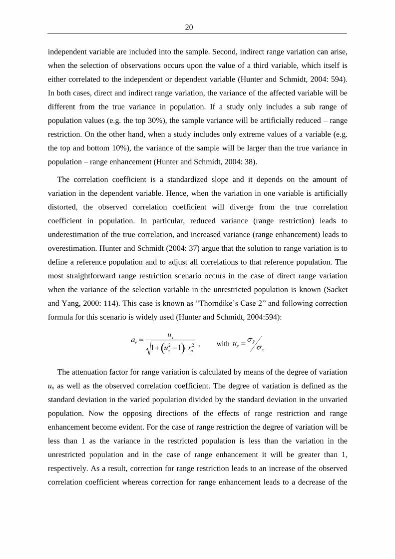
and Yang, 2000: 114). This case is known as “Thorndike’s Case 2” and following correction

formula for this scenario is widely used (Hunter and Schmidt, 2004:594):

ar ux

1 ux

2 1 ro

2 , with

ux ̃x

x

The attenuation factor for range variation is calculated by means of the degree of variation

ux as well as the observed correlation coefficient. The degree of variation is defined as the

standard deviation in the varied population divided by the standard deviation in the unvaried

population. Now the opposing directions of the effects of range restriction and range

enhancement become evident. For the case of range restriction the degree of variation will be

less than 1 as the variance in the restricted population is less than the variation in the

unrestricted population and in the case of range enhancement it will be greater than 1,

respectively. As a result, correction for range restriction leads to an increase of the observed

correlation coefficient whereas correction for range enhancement leads to a decrease of the

21

observed correlation coefficient. Figure 5 illustrates the effects of the degree of variation on

the correction for range variation for different observed correlation coefficients.

Figure 5: The Effect of Range Variation

Additionally, in contradiction to the correction for measurement error and for

dichotomization of a continuous variable, the correction for range variation has to be

considered as a special case. The attenuation factors for the former artifacts are entirely

determined by the extent of the artifact itself; however, the attenuation factor for range

variation is additionally dependent upon the size of the observed correlation. Mendoza and

Mumford argue (1987) that the true values and errors of measurement in the restricted

population are negatively correlated in presence of direct range restriction; hence the meaning

of reliability becomes unclear for the independent variable measure. This problem can be

solved by adherence to an order principle: correction for range restriction must be introduced

after correction for error of measurement. If the correction for range variation is applied to

the correlation that has already been corrected for error of measurement, the hypothetical case

on non-existence of measurement error occurs, and only then will the correction for range

restriction be accurate (Hunter and Schmidt, 2004: 597).

22

More complex scenarios arise in the presence of indirect range variation and simultaneous

range variation on both dependent and independent variable. Since their detailed illustration

goes beyond the scope of this paper, we will only direct the reader’s attention to possible

solutions in the literature. If the variance of the third selection variable in the unvaried

population is known, indirect range variation is known as “Thorndike’s Case 3” and

correction formulae are available (Sacket and Yang, 2000: 115). However, this information is

unknown in most research, which is why Hunter et al. (2006: 599-604) have presented a

seven-step correction method that does not rely upon this information. Correction for

simultaneous range variation poses an unsolvable complexity, for which there are at present

no exact statistical methods (Hunter and Schmidt, 2004: 40). However, Alexander et al.

(1987: 309-315) have presented approximation methods for the effect of double range

variation.

3.3 Unavailability of Artifact Information and Multiple Artifacts

If all necessary information is known for all included studies, the correction for each

observed correlation coefficient can be achieved according to the presented methods.

Unfortunately, this information is often not available in meta-analysis (Lipsey and Wilson,

2001: 108). Nevertheless, if the artifact information is available for nearly all individual

studies, the missing data can be estimated by the mean values of the present artifact

information (Hunter and Schmidt, 2004: 121). If this is not the case and artifact information

is only available sporadically, the meta-analyst has to decide whether to adjust some effects

while leaving others unadjusted, or to leave all effects unadjusted and thus ignoring the

effects of study imperfection. In the latter case, the estimation of the population correlation

will be a biased estimation and therefore a very poor estimation of the reality (Hunter and

Schmidt, 2004: 132).

Hunter and Schmidt (2004: 137-188) have presented a method of meta-analysis of

correlation coefficients using artifact distribution. This method enables the meta-analyst to

correct for study imperfections on the aggregate level, after conduction of a bare-bones meta-

analysis. When applying a meta-analysis of correlation coefficients using artifact distribution,

the estimation of the population correlation will still be an underestimate of the reality,

however, the results will be much more accurate than the results of a bare-bones meta-

23

analysis. We recommend caution in the context of ignoring the impact of study imperfection

and advise meta-analysts to apply the methods of meta-analysis using artifact distributions.

The preceding sections have illustrated the effects of various artifacts and have presented

attenuation factors that reflect the individual effect of the study imperfection on the observed

correlation coefficient. In reality, study imperfections will arise simultaneously and hence

methods to take multiple simultaneous artifacts into account need to be considered.

Measurement error and dichotomization of a continuous variable only depend on

individual study imperfections and have a causal structure that is independent of that for other

artifacts. Hence, the compound effect of these artifacts behaves multiplicative and a

compound attenuation factor can be described as the simple product of individual attenuation

factors (Hunter and Schmidt, 2004: 118): A = am ad. However, in the case of range variation

on either the dependent or the independent variable, a different method to compute the

compound attenuation factor has to be used. This is due to the negative correlation of true

scores and measurement error in presence of range variation as described above (Hunter and

Schmidt, 2004: 597):

a r ux

1 (ux

2 1) ro

am

2

A amada r

An accurate compound attenuation factor will only be retrieved if the observed correlation

is corrected for measurement error before computing the attenuation factor for range

variation. Hence, the attenuation factor for range variation must be modified by inclusion of

the attenuation factor for measurement error. After this correction, the modified compound

attenuation factor A’ of all three artifacts can then be computed.

To conclude, individual study correlations can now be corrected for measurement error,

error due to artificial dichotomization, and direct range variation. The corrected correlation

can be obtained by the quotient of observed correlation and the compound attenuation factor,

as follows:

rc ro

A

24

4 Aggregating Effect Sizes across Studies

In the preceding section we focused individual study computations and showed how in a

first step individual study findings can be transformed to a comparable effect size

measurement and be corrected for study imperfections. In this section we describe the

statistical methods for the estimation of the population correlation and the estimation of the

variance in population correlation on the aggregated level. In this context, the impact of

sampling error in individual studies on the estimators on the aggregated level will be

discussed and methods to correct the estimators are presented.

4.1 Estimating the Population Correlation

Besides the estimation of the true correlation between a dependent and an independent

variable, meta-analysis aims to estimate the variance of this estimation (Johnson et al., 1995:

95). When analyzing this variance, meta-analysis can in particular address the question,

whether the estimation of the population correlation is an estimate of a single underlying

population or various sub populations (Cheung and Chan, 2004: 780). A central fact in this

context is that results of study findings can differ significantly, even though all studies are

consistent with a single underlying effect size (Franke, 2001: 187). This is caused by

presence of sampling error (Franke, 2001: 187; Hunter and Schmidt, 2004: 34; Viechtbauer,

2007: 29).

To understand the effects of sampling error, consider a meta-analysis that only

incorporates replications of a single study drawn from different samples of the same

population. The true correlation in population will be identical for all replications. However,

the observed correlation for each replication will vary only because each sample will consist

of different observations as a result of the random sample selection process. Therefore, in an

individual study, the observed correlation coefficient can be described as the summation of

the true population correlation and an error term – sampling error (Hunter and Schmidt, 2004:

84). Sampling error occurs unsystematically and its effect on the observed correlation

coefficient reported in a single study is unobservable. However, the effects of sampling error

become observable and furthermore correctable when combining individual study

observations to an overall measurement on the aggregated level of meta-analysis. The

variance of the sampling error in the individual study will from now on be denoted as study

25

sampling error variance. In theory, the standard deviation of the sampling error in a single

study can be calculated as follows (Hunter and Schmidt, 2004: 85):

(e) 1 2

N 1

As the standard deviation of the sampling error in a single study is dependent on the

unknown population correlation, it resides theoretical at first.

Since the error term in the individual correlation coefficient is random and unpredictable,

it will in some cases enlarge the true correlation coefficient and in some cases reduce the true

correlation coefficient. Hence, if individual study findings were to be averaged to a mean

correlation coefficient, sampling error would partially neutralize itself. As a result, the simple

average of all individual correlations will be less affected by sampling error than the

individual study findings, and the average will be closer to the true population correlation

than the individual study findings. However, it is not the simple average of the corrected

correlations that will lead to the best estimation of the population correlation.

As different studies will vary in precision and in the extent of study imperfection, a much

better estimation of the population correlation can be retrieved when taking those differences

into account. Meta-analysis therefore makes use of a weighted average. The optimal weight

for each individual study is the inverse of sampling error variance (Lipsey and Wilson, 2001:

36; Cheung and Chan, 2004: 783). Hence, as a larger sampling error corresponds to a less

precise effect size value (Lipsey and Wilson, 2001: 36), a weighting scheme on the basis of

the inverse sampling error variance gives a greater weight to precise studies and less weight

to imprecise studies. Hunter and Schmidt (2004: 124) go on and argue that in the case of

great variation in artifact correction throughout studies, a more complicated weighting

scheme accounting for these differences will lead to a better estimation of the population

correlation. They therefore extend the weighting scheme by multiplying the inverse sampling

error variance with the squared compound attenuation factor. This way, the weighting scheme

accounts for both, unequal sample sizes, as well as the quality of study findings (Hunter and

Schmidt, 2004: 125). However, in order to calculate the sampling error variance in an

individual study, the true underlying population correlation is required. This population

correlation can be estimated by the simple average of the observed correlation coefficient

across studies (Hunter and Schmidt, 2004: 123). As this estimation is equal for all included

26

studies, the numerator of the sampling error variance is identical for each study and can

therefore be dropped from the weight formula:

wi Ni 1 Ai

2

As a result, the mean corrected correlation can be estimated by weighting each corrected

correlation with the respective study weight. This weighted mean corrected correlation serves

to the end of the estimation of the population correlation.

ˆ r c

wirc.i

i1

k

wi

i1

k

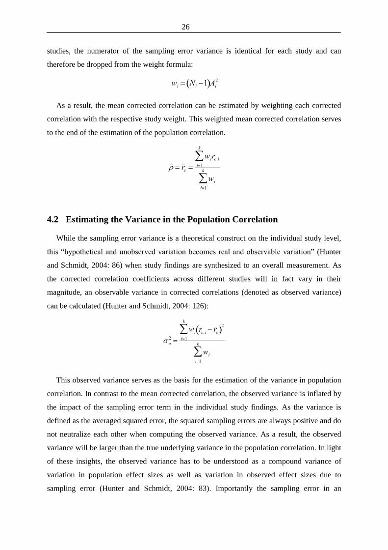
4.2 Estimating the Variance in the Population Correlation

While the sampling error variance is a theoretical construct on the individual study level,

this “hypothetical and unobserved variation becomes real and observable variation” (Hunter

and Schmidt, 2004: 86) when study findings are synthesized to an overall measurement. As

the corrected correlation coefficients across different studies will in fact vary in their

magnitude, an observable variance in corrected correlations (denoted as observed variance)

can be calculated (Hunter and Schmidt, 2004: 126):

o

2

wi rc.i r c 2

i1

k

wi

i1

k

This observed variance serves as the basis for the estimation of the variance in population

correlation. In contrast to the mean corrected correlation, the observed variance is inflated by

the impact of the sampling error term in the individual study findings. As the variance is

defined as the averaged squared error, the squared sampling errors are always positive and do

not neutralize each other when computing the observed variance. As a result, the observed

variance will be larger than the true underlying variance in the population correlation. In light

of these insights, the observed variance has to be understood as a compound variance of

variation in population effect sizes as well as variation in observed effect sizes due to

sampling error (Hunter and Schmidt, 2004: 83). Importantly the sampling error in an

27

individual study is independent from the underlying population effect size, which means that

the covariance of sampling error and population effect must be zero (Hunter and Schmidt,

2004: 86). The observed variance can therefore be decomposed into a true variance in

population correlation component and a component due to sampling error variance across

studies, as follows:

o

2 2 e

2

It becomes evident that the key concept in estimating the true variance in population

correlation is to estimate the sampling error component of the observed variance. This

variance is just the average of all study sampling error variances.

In this context, the artifact correction due to study imperfection has an additional effect on

the estimations. When the multiplicative correction process for artifact attenuation is applied

to the observed correlation, both the true correlation and the sampling error term in the

observed correlation are enlarged. Hence, the artifact correction process does not only adjust

the observed correlation, but also amplifies the error term in the same manner, and

subsequently enlarges the sampling error variance (Hunter and Schmidt, 2004: 96).

Therefore, when estimating the study sampling error variance, the study sampling error

variance in uncorrected correlations has to be estimated in a first step, and in a second step

has to be adjusted for the amplification effect of artifact correction. Hunter and Schmidt

(2004: 88) have derived an estimator for the study sampling error variance in uncorrected

correlations based on the mean uncorrected correlation and the sample size of the respective

study. As the artifact correction amplifies the sampling error term by the factor

1 Ai , the effect

on the variance is described by the factor

1 Ai

2 . Hence, the study sampling error variance in

corrected correlations can be estimated by an analogous amplification of the study sampling

error variance in the uncorrected correlation:

2(e)i (1 r o

2)2

N i 1

c

2(e)i 2(e)i

Ai

2

28

Now, the sampling error variance across studies can be estimated by the average study

sampling error variance in corrected correlations (Hunter and Schmidt, 2004: 126):

e

2

wi c

2 e i

i1

k

wi

i1

k

Due to the independence of sampling error term and the underlying correlation in each

study, the estimation of the variance in the population correlation can now be performed by

simply deducting the sampling error variance across studies from the observed variance in a

final step:

ˆ 2 o

2 e

2

Aguinis (2001: 584) has assessed the performance of the sampling error variance estimator

by Hunter and Schmidt and comes to the conclusion that the estimator outperforms

previously applied estimators. However, although the estimator provided by Hunter and

Schmidt improves negative bias, it shall be retained that the estimation of sampling in some

cases tends to an underestimation (Hunter and Schmidt, 2004: 168).

4.3 Dependent Effect Sizes

The presented meta-analytical methods on the aggregated level are based on the

assumption that the reported study findings are independent (Martinussen and Bjornstad,

1999: 928; Cheung and Chan, 2004: 780). This assumption is frequently violated in meta-

analysis. If a study reports more than one correlation coefficient or different studies are based

on the same sample, the reported correlation coefficients will be dependent because of factors

such as response sets or other sample specific characteristics (Cheung and Chan, 2004: 781).

The effects on meta-analytical outcomes become evident when analyzing the estimators

for the population correlation and the variance in population correlation. If dependent effect

sizes are included into meta-analysis, the same effect is essentially given multiple weighting

in the estimation of the population correlation. Hence, the estimation will be biased towards

the magnitude of the dependent effect sizes. On the other hand, the estimation of the variance

in population correlation will be affected if the study sampling error variance in the

dependent effect sizes differs from the average study sampling error variance in every other

29

effect size. Since the sampling error variance across studies is defined as the average study

sampling error variance, it will be overestimated if study sampling error variance in the

dependent effect size is above average, and, underestimated if it is below average.

The common procedure in meta-analysis is to compute a within-sample average across the

dependent effect sizes before inclusion into meta-analytical estimations (Martinussen and

Bjornstad, 1999: 929; Cheung and Chan, 2004: 782). Through this step it can be ensured that

all effect sizes included into meta-analysis are independent, and at the same time no available

data has to be discarded. However, one could argue that a within-sample average based on

more than one correlation coefficient is a more precise measurement than a single correlation

coefficient and hence has a smaller study sampling error variance. The answer lies in the

degree of interdependence between coefficients. The more they are independent, the more

precise will be the average, which should be reflected in the weighting scheme. In the

extreme case of totally independent correlations, they could be treated as if they came from

different samples. In reality, the correlation between two coefficients arising from the same

sample will lie somewhere on the continuum between 0 and 1.00. Therefore, if (partially)

dependent correlation coefficients are combined to a within-sample average, the sampling

error variance across studies will be overestimated and consequently the variance in

population correlation will be underestimated (Cheung and Chan, 2004: 782). In order to

counteract this underestimation, it is recommended to follow the procedures of Cheung and

Chan (2004: 782) for incorporating the degree of interdependence in meta-analysis,

especially when averaging occurs frequently.

5 Homogeneity Tests and Moderator Analysis

In addition to the quantification of the relationship between the dependent and the

independent variables in population, meta-analysis furthermore addresses the question of

whether included effect sizes belong to the same population (the homogeneous case), and if

not (the heterogeneous case), what factors explain the observed variation (Whitener, 1990:

315; Sanchez-Meca and Marin-Martinez, 1997: 386; Franke, 2001: 188; Cheung and Chan,

2004: 780). Therefore, after aggregating the effect sizes to an average effect size, the

application of homogeneity tests is necessary. Homogeneity tests are in general based on the

fact that the observed variance is made up of variance due to true variation in population

correlation and variance due to sampling error. Due to the fact that the estimated variance in

30

population correlation is corrected for sampling error, it represents the amount of variability

in the observed variance beyond the amount that is expected from sampling error alone

(Viechtbauer, 2007: 30).

5.1 The Concept of Heterogeneity

If the estimated variance in population correlation (residual variance) is equal to zero, the

meta-analyst can assume homogeneity, as the observed variance is described by sampling

error alone (Whitener, 1990: 316; Aguinis, 2001: 572). However, if the estimation of the

variance in population correlation is greater than zero, three possible scenarios arise: first the

residual variance can be described by true variability, second the residual variance can be

described by artificial variability that has not been taken into account yet, and third the

residual variance can be described by a combination of the former two (Lipsey and Wilson,

2001: 116-118). In the case of true residual variability the meta-analyst has to assume

heterogeneity (Aguinis, 2001: 572). Then a moderator analysis can be applied in order to

illuminate heterogeneity in findings, allowing for further testing of details in the examined

research field (Rosenthal and DiMatteo, 2001: 74; Hedges and Pigott, 2004: 426). A

moderator variable has to be understood as a variable that “affects the direction and/or the

strength of the relationship between an independent or predictor variable and a dependent or

criterion variable” (Baron and Kenny, 1986: 1174).

However, there are numerous other sources that can potentially cause additional artificial

variability. These range from simple errors, such as computational, typographical and

transcription errors (Sagie and Koslowsky, 1993: 630), to empirical errors such as a possible

underestimation of the sampling error variance across studies as well as error associated with

the sampling process on the aggregate level of meta-analysis. Hunter and Schmidt (2004:

411) denote the latter error as second-order sampling error. If a random-effects model is

assumed, not only individual study findings are affected by random sample selection, but also

the aggregate estimates themselves are exposed to (second–order) sampling error. Consider

the case that every available study in a particular research domain has an indefinite sample

size. Sampling error in every individual study would diminish, and hence every study would

report the true but different (random-effects model) underlying correlation. As a result, the

meta-analytical estimates may vary only due to a random selection process; just like

individual study findings are affected by sampling error if their sample size is not indefinite.

31

For that reason, the hypothetical case of a negative residual variance can arise. In that case,

the residual variance can then be treated as if it were equal to zero (Hunter and Schmidt,

2004: 89). Furthermore, e.g. when additional artificial variation is present in the meta-

analysis or when the sampling error variance across studies is underestimated, the residual

variance can be greater than zero although homogeneity underlies.

On average 72% of the observed variance among studies is artificially caused by sampling

error, error of measurement and range variation alone (Sagie and Koslowsky, 1993: 630).

Based on this insight Hunter and Schmidt (2004: 401) have derived a rule of thumb for

assessing homogeneity in meta-analysis: If more than 75% of the observed variance is due to

artifacts, it is likely that the remaining variance is caused by additional artifacts that have not

been taken into account. Hence they suggest that homogeneity in study findings can be

assumed if the ratio of sampling error variance and observed variance exceeds the critical

value of 75% (Sagie and Koslowsky, 1993: 630; Sanchez-Meca and Marin-Martinez, 1997:

387).

In addition to Hunter and Schmidt’s rule of thumb, various statistical tests can be applied

in order to assess whether the observed variance is based on artificial variance or true

variance. The most frequently used homogeneity tests in meta-analysis are the

Q-test and the application of credibility intervals around the estimated population correlation

(Sagie and Koslowsky, 1993: 630; Sanchez-Meca and Marin-Martinez, 1997: 387; Aguinis,

2001: 584).

5.2 The Q-Test

When conducting a

Q-Test, the meta-analyst postulates the null hypothesis that the true

underlying correlation coefficient is identical for every study that is included into the meta-

analysis. Hence the null hypothesis embodies the assumption of homogeneity. In the case that

all studies in fact have the same underlying population correlation, the test statistic

Q follows

a chi-square distribution with

k 1 degrees of freedom (Sanchez-Meca and Marin-Martinez,

1997: 386; Hedges and Vevea, 1998: 490; Lipsey and Wilson, 2001: 115; Field, 2003: 110;

Viechtbauer, 2007: 35):

Q wi

i1

k

rc.i r c , with

Q

2 k 1

32

A significant

Q statistic is therefore a sign for heterogeneity. However, the distribution of

the

Q statistic only becomes exactly chi-squared distributed when all the sample sizes of all

studies become large (Viechtbauer, 2007: 35). Although various authors suggest that the

Q-

test generally keeps the type I error rate close to the nominal

-value, Sánchez-Meca and

Martín-Martínez (1997: 393) have shown that the type I error rate for the

Q-test is

substantially higher than the initially defined α-level in the case of small study sample sizes.

Furthermore, when the

Q-test cannot reject the null hypothesis, and meta-analysts believe in

homogeneity, they do so with an unknown type II error rate. This type II error rate is

dependent on the nominal α-level, the degree of heterogeneity, the number of studies

included into meta-analysis and the sample sizes of each study. In this context, Sánchez-

Meca and Martín-Martínez (1997: 396) have shown that even with extreme heterogeneity

across studies and a reasonable α-level of 0.05, the power of the

Q-test to detect this

heterogeneity can be as low as 24.9% when the number of studies (6) and the average sample

size (30) are low. On the other hand, when the number of studies is large, the

Q-test will

reject the null hypothesis among studies even in the case of a trivial departure from

homogeneity such as departures from artifact uniformity across studies (Hunter and Schmidt,

2004: 416). For both reasons Hunter and Schmidt discourage meta-analysts to apply the

Q-

test statistics.

The

Q-test can be powerful to disprove homogeneity in case the sample sizes in the

studies are not too small. However, the

Q-test should not be used to conclude homogeneity

amongst studies. In the case that the

Q-test cannot reject the null hypothesis, the meta-analyst

has to be aware that the probability of heterogeneity amongst studies is still comparatively

high. Therefore, the meta-analyst should apply credibility intervals in addition to the

Q-test

and the 75% rule of thumb.

5.3 The Credibility Interval

When assessing homogeneity with the use of a credibility interval, the meta-analyst

creates a range in which underlying population correlations are likely to be positioned. By

means of this interval the meta-analyst can then conclude whether the underlying population

correlations are identical, similar or greatly different in magnitude.

x1,2 ˆ (1 2) ˆ

33

The credibility interval refers to the distribution of parameter values, rather than a single

value (Hunter and Schmidt, 2004: 205), as it is the case when assessing the reliability of a

point estimator with a confidence interval. Hence, the credibility interval is constructed with

the posterior distribution of effect sizes that results after corrections for artifacts have been

made and does not depend on sampling error (Whitener, 1990: 317). A credibility interval

can be computed around the estimation of the population correlation using the estimation of

the standard deviation of the population correlation. If this interval is relatively large or

includes zero, the meta-analyst has then to assume that the estimation of the population

correlation is probably an average of several subpopulation correlations. One can therefore

conclude heterogeneity and has to believe that moderators are operating. However, if on the

other hand the credibility interval is comparably small and/or does not include zero, the

estimation of the population correlation is probably the estimate of a single underlying

population (Whitener, 1990: 317).

It becomes obvious that a credibility interval facilitates a higher personal interpretability

than the

Q-test. It is upon the meta-analysts judgment, which size of credibility can be

referred to as small, and which as large. Nonetheless, this interpretability entails advantages

as well. E.g., when credibility intervals are comparably large, the meta-analyst must conclude

that the examined effect is still greatly moderated by effects that have not been taken into

account yet. However, if this credibility interval does not include zero, one can furthermore

conclude that the moderating effects have only little influence on the direction of the

examined effect. One could therefore postulate that the examined relationship is on average

positive (or negative) but furthermore only the precise magnitude is affected by moderators.

6 Interpretation of Meta-Analytic Results

To sum up, in the case of heterogeneous findings, the meta-analyst must conclude that the

relationship between the examined variables is not universal but rather dependent on

moderating effects. If credibility intervals do not include zero, the meta-analyst could

conclude that the direction of an effect is – on average – positive or negative. However, in the

case that the meta-analyst can conclude homogeneity among study findings, one could

possibly make a generalized statement about the examined relationship. In order to ensure

that the conclusions drawn from the obtained meta-analytical findings are appropriate, a

generalized statement should only be made after addressing the question of validity and

34

reliability of the meta-analytic estimations. Reliability refers to the question, whether the

meta-analytic results could be based on chance, and validity refers to the question, whether

the results of meta-analysis reflect reality (Carmines and Zeller, 1979: 10).

The first question can be answered by application of a confidence interval (Whitener,

1990: 316). As depicted, in the case of homogeneity, the observed variation among studies is

only due to sampling error. Hence, the confidence interval around the estimation of the

population correlation can be constructed using the standard error of the estimation of the

population correlation (Hunter and Schmidt, 2004: 206). Although formulas for the standard

error of the estimation of the population correlation are complex, Hunter and Schmidt have

provided a simple and fairly accurate approximation:

SE ̂ o k

y1,2 ˆ (1 2) SE ̂

Now, the upper and lower boundary of the confidence interval with a type I error rate of α

can be computed. If the confidence interval excludes zero, the meta-analyst can then

conclude that the estimated population correlation is unlikely to be based on chance and is

therefore reliable. However, Hunter and Schmidt (2004: 206) argue that the application of

confidence intervals in meta-analysis only plays a subordinate role and that the application of

credibility intervals is of higher importance.

The latter question whether meta-analytic results are valid, seeks for the endeavor of

generalization of validity. “The generalization of validity refers to whether situational

differences influence the value of a test in a predicting performance” (Whitener, 1990: 315).

Hence, an important prerequisite towards generalization of validity of meta-analytic results is

homogeneity across individual study findings. If underlying studies are heterogeneous, no

general statement about the relationship between the examined variables can be made, as

unknown effects moderate the relationship. Nevertheless, Hunter et al. (1982) argue that once

artifacts have been eliminated from meta-analytic estimations, the “theorist is provided with a

very straightforward fact to weave into the overall picture”.

However, there are possible threats to the validity in meta-analysis. The most striking

threat is the described “file drawer problem” (Sutton et al., 2001: 142). In the case that the

meta-analyst cannot obtain studies that show non-significant results, the validity of meta-

analytical findings might be questionable because these inaccessible studies might have

35

altered findings. Rosenthal has developed a formula that computes the number of non-

significant study findings (“Fail-Safe N”) that “must be in the file drawers“ (Rosenthal, 1979:

639) before the probability of a type I error of a significance test would increase to an

unjustifiable level. Based on this framework, Orwin (1983: 158) has modified Rosenthal’s

formula and has presented a “Fail-Safe N” calculation formula that applies to Cohen’s effect

size

d . The modified computation formula is therefore unattached to the type I error

probability and rather calculates the number of studies that is needed to alter the observed

effect size to a different value, which is denoted as criterion effect size level. Carson and

Schriesheim (1990: 234) argue that the computation formula can be used not only to assess

whether meta-analytical findings are affected by publication bias, but to generally assess the

stability of findings in meta-analysis. Therefore, they interpret the “Fail-Safe N” in a broader

way as the number of new, unpublished, or unretrieved results that would alter the observed

effect size to the criterion effect size level. Orwin’s “Fail-Safe N” can be calculated as

follows (Orwin, 1983: 158):

X kdo dc

dc d fs

In Orwin’s “Fail-Safe N” formula,

k is the number of studies in the meta-analysis,

do is

the observed effect size,

dc is the criterion effect size and

d fs is the assumption that the meta-

analyst wishes to make about the missing effect sizes. If meta-analysts want to validate

findings against publication bias, they consequently assume

d fs 0. However, the meta-

analyst can make any other reasonable assumption about missing effect sizes and assess how

many studies of such kind would be needed to alter the observed effect size to the criterion

effect size.

When the transformation formula between the effect size r and effect size d is reversed,

the effect size d can be obtained from the effect size r (Rosenthal and DiMatteo, 2001: 71).

Hence, when meta-analysts transform the estimation of the population correlation to the

equivalent d-value, they can then apply the presented formulae for computation of “Fail-Safe

N” statistics to the meta-analytic findings (Lipsey and Wilson, 2001: 166). When applying

“Fail-Safe N” computations, the meta-analyst has then to specify a criterion effect size that

she believes would question the validity of findings. In this context, Carson and Schriesheim

(1990: 237) use Cohen’s (1969) widely recognized classification of small (0.2), medium

(0.5), and large (0.8) effect sizes and regard “important” or “significant” alterations as a

36

reduction of the initial finding to the next lower criterion level (e.g., from large to medium, or

from medium to small). The implementation of these methods allows the meta-analyst to

compute “Fail-Safe N” statistics in order to assess the stability of meta-analytical findings.

Cohen’s convention for means can also be used to interpret correlation coefficients. When

the classifications of small, medium, and large effect sizes are transformed to a correlation

coefficient, the analogous values translate to 0.10, 0.25 and 0.37, respectively (Carson and

Schriesheim, 1990: 237). Lipsey and Wilson (2001: 147) therefore advise the meta-analyst to

interpret the estimation of the population correlation as small effect in the case the magnitude

is below 0.10, as medium effect in case the magnitude ranks around 0.25 and as large effect

when the magnitude of the estimated population correlation is greater than 0.37.

Despite the many advantages of meta-analysis, the meta-analytical techniques require

advanced statistical knowledge and many scholars fail to apply appropriate methods that

account for random variation and study imperfections among primary study findings. This

paper provided a guideline to the meta-analysis of correlation coefficients from the first step

of transforming different statistical measures to a comparable effect size over methods to

correct primary study findings for sampling error, error of measurement, dichotomization,

and range variation to the final step of estimating the relationship between the investigated

variables and assessment of homogeneity among the meta-analytical findings.

37

References

Aguinis, H. (2001). Estimation of Sampling Variance of Correlations in Meta-Analysis.

Personnel Psychology, 54, 3, 569-590.

Alexander, R. A., Carson, K. P., Alliger, G. M., Carr, L. (1987). Correcting Doubly

Truncated Correlations - an Improved Approximation for Correcting the Bivariate

Normal Correlation When Truncation Has Occured on Both Variables. Educational &

Psychological Measurement, 47, 2, 309-315.

Baron, R. M., Kenny, D. A. (1986). The Moderator-Mediator Variable Distinction in Social

Psychological Research: Conceptual, Strategic, and Statistical Considerations. Journal

of Personality and Social Psychology, 51, 6, 1173-1182.

Bortz, J., Döring, N. (2002). Forschungsmethoden Und Evaluation. Springer: Berlin.

Carmines, E. G., Zeller, R. A. (1979). Reliability and Validity Assessment. Sage

Publications: Beverly Hills.

Carson, K. P., Schriesheim, C. A. (1990). The Usefulness of the 'Fail Safe' Statistic in Meta-

Analysis. Educational & Psychological Measurement, 50, 2, 233-243.

Cheung, S. F., Chan, D. K. S. (2004). Dependent Effect Sizes in Meta-Analysis:

Incorporating the Degree of Interdependence. Journal of Applied Psychology, 89, 5,

780-791.

Cohen, J. (1969). Statistical Power Analysis for the Behavioural Sciences. Academic Press:

New York.

Cooper, H. M., Hedges, L. V. (1994). Research Synthesis as a Scientific Enterprise. In:

Cooper, H. M., Hedges, L. V. (Eds.), The Handbook of Research Synthesis, New York:

Russell Sage Foundation, 3-14.

Egger, M., Smith, G. D. (1997). Bias in Meta-Analysis Detected by a Simple, Graphical Test.

British Medical Journal, 315, 7109, 629-634.

Field, A. P. (2003). The Problem in Using Fixed-Effects Models of Meta-Analysis on Real-

World Data. Understanding Statistics, 2, 2, 105-124.

Franke, G. R. (2001). Applications of Meta-Analysis for Marketing and Public Policy: A

Review. Journal of Public Policy & Marketing, 20, 2, 186-200.

Fricke, R., Treinies, G. (1985). Einführung in Die Metaanalyse. Huber: Bern.

Glass, G. V., McGaw, B., Smith, M. L. (1981). Meta-Analysis in Social Research. Sage

Publications: Beverly Hills.

Gliner, J. A., Morgan, G. A., Harmon, R. J. (2003). Meta-Analysis: Formulation and

Interpretation. Journal of the American Academy of Child & Adolescent Psychiatry, 42,

11, 1376-1379.

38

Gross, A. L., McGanney, M. L. (1987). The Restriction of Range Problem and Nonignorable

Selection Process. Journal of Applied Psychology, 72, 4, 604-610.

Halvorsen, K. T. (1994). The Reporting Format. In: Cooper, H., Hedges, L. V. (Eds.), The

Handbook of Research Synthesis, New York: Russell Sage Foundation, 425-437.

Hedges, L. V. (1992). Meta-Analysis. Journal of Educational Statistics, 17, 4, 279-296.

Hedges, L. V., Gurevitch, J. (1999). The Meta-Analysis of Response Ratios in Experimental

Ecology. Ecology, 80, 4, 1150.

Hedges, L. V., Olkin, I. (1985). Statistical Methods for Meta-Analysis. Academic Press:

Orlando.

Hedges, L. V., Pigott, T. D. (2004). The Power of Statistical Tests for Moderators in Meta-

Analysis. PSYCHOLOGICAL METHODS, 9, 4, 426-445.

Hedges, L. V., Vevea, J. L. (1998). Fixed- and Random-Effects Models in Meta-Analysis.

PSYCHOLOGICAL METHODS, 3, 4, 486-504.

Hunter, J. E., Schmidt, F. L. (1990). Methods of Meta-Analysis: Correcting Error and Bias in

Research Findings. Sage Publications: Newbury Park.

Hunter, J. E., Schmidt, F. L. (2004). Methods of Meta-Analysis : Correcting Error and Bias in

Research Findings. Sage: Thousand Oaks, CA.

Hunter, J. E., Schmidt, F. L., Jackson, G. B. (1982). Meta-Analysis Cumulating: Research

Findings across Studies. Sage Publications: Beverly Hills.

Hunter, J. E., Schmidt, F. L., Le, H. (2006). Implications of Direct and Indirect Range

Restriction for Meta-Analysis - Methods and Findings. Journal of Applied Psychology,

91, 3, 594-612.

Johnson, B. T., Mullen, B., Salas, E. (1995). Comparison of Three Major Meta-Analytic

Approaches. Journal of Applied Psychology, 80, 1, 94-106.

Lipsey, M. W., Wilson, D. B. (2001). Practical Meta-Analysis. Sage Publications: Thousand

Oaks, Calif.

MacCallum, R. C., Zhang, S., Preacher, K. J., Rucker, D. D. (2002). On the Practice of

Dichotomization of Quantitative Variables. PSYCHOLOGICAL METHODS, 7, 1, 19-

40.

Mann, C. (1990). Meta-Analysis in the Breech. Science, 249, 4968, 476-480.

Martinussen, M., Bjornstad, J. F. (1999). Meta-Analysis Calculations Based on Independent

and Nonindependent Cases. Educational & Psychological Measurement, 59, 6, 928-

950.

Mendoza, J. L., Mumford, M. (1987). Correction for Attenuation and Range Restriction on

the Predictor. Journal of Educational Statistics, 12, 3, 282-293.

39

Moayyedi, P. (2004). Meta-Analysis: Can We Mix Apples and Oranges? American Journal

of Gastroenterology, 99, 12, 2297-2301.

Muncer, S. J., Craigie, M., Holmes, J. (2003). Meta-Analysis and Power: Some Suggestions

for the Use of Power in Research Synthesis. Understanding Statistics, 2, 1, 1-12.

Orwin, R. G. (1983). A Fail-Safe N for Effect Size in Meta-Analysis. Journal of Educational

Statistics, 9, 2, 157-159.

Peterson, R. A., Brown, S. P. (2005). On the Use of Beta Coefficients in Meta-Analysis.

Journal of Applied Psychology, 90, 1, 175-181.

Rosenthal, R. (1979). The File Drawer Problem and Tolerance for Null Results.

Psychological Bulletin, 86, 3, 638-641.

Rosenthal, R. (1991). Meta-Analytic Procedures for Social Research. Sage Publications:

Newbury Park.

Rosenthal, R., DiMatteo, M. R. (2001). Meta-Analysis: Recent Developments in Quantitative

Methods for Literature Reviews. Annual Review of Psychology, 52, 1, 59-82.

Rosenthal, R., Rubin, D. (1978). Interpersonal Expectancy Effects: The First 345 Studies.

Behavioural and Brain Sciences, 3, 377-415.

Rosenthal, R., Rubin, D. (1988). Comments: Assumptions and Procedures in the File Drawer

Problem. Statistical Science, 3, 120-125.

Sacket, P. R., Yang, H. (2000). Correcting for Range Restriction: An Expanded Typology.

Journal of Applied Psychology, 85, 1, 112-118.

Sagie, A., Koslowsky, M. (1993). Detecting Moderators with Meta-Analysis: An Evaluation

and Comparison of Techniques. Personnel Psychology, 46, 3, 629-640.

Sanchez-Meca, J., Marin-Martinez, F. (1997). Homogeneity Tests in Meta-Analysis: A

Monte Carlo Comparison of Statistical Power and Type I Error. Quality & Quantity, 31,

4, 385-399.

Smith, M. L., Glass, G. V., Miller, T. I. (1980). The Benefits of Psychotherapy. Johns

Hopkins University Press: Baltimore (MD).

Song, F., Sheldon, T. A., Sutton, A. J., Abrams, K. R., Jones, D. R. (2001). Methods for

Exploring Heterogeneity in Meta-Analysis. Evaluation & the Health Professions, 24, 2,

126-151.

Sutton, A. J., Abrams, K. R., Jones, D. R. (2001). An Illustrated Guide to the Methods of

Meta-Analysis. Journal of Evaluation in Clinical Practice, 7, 2, 135-148.

Viechtbauer, W. (2007). Hypothesis Tests for Population Heterogeneity in Meta-Analysis.

British Journal of Mathematical & Statistical Psychology, 60, 1, 29-60.

Whitener, E. M. (1990). Confusion of Confidence-Intervals and Credibility Intervals in

Metaanalysis. Journal of Applied Psychology, 75, 3, 315-321.