xavier raynaud- on a shallow water wave equation
TRANSCRIPT
8/3/2019 Xavier Raynaud- On a Shallow Water Wave Equation
http://slidepdf.com/reader/full/xavier-raynaud-on-a-shallow-water-wave-equation 1/161
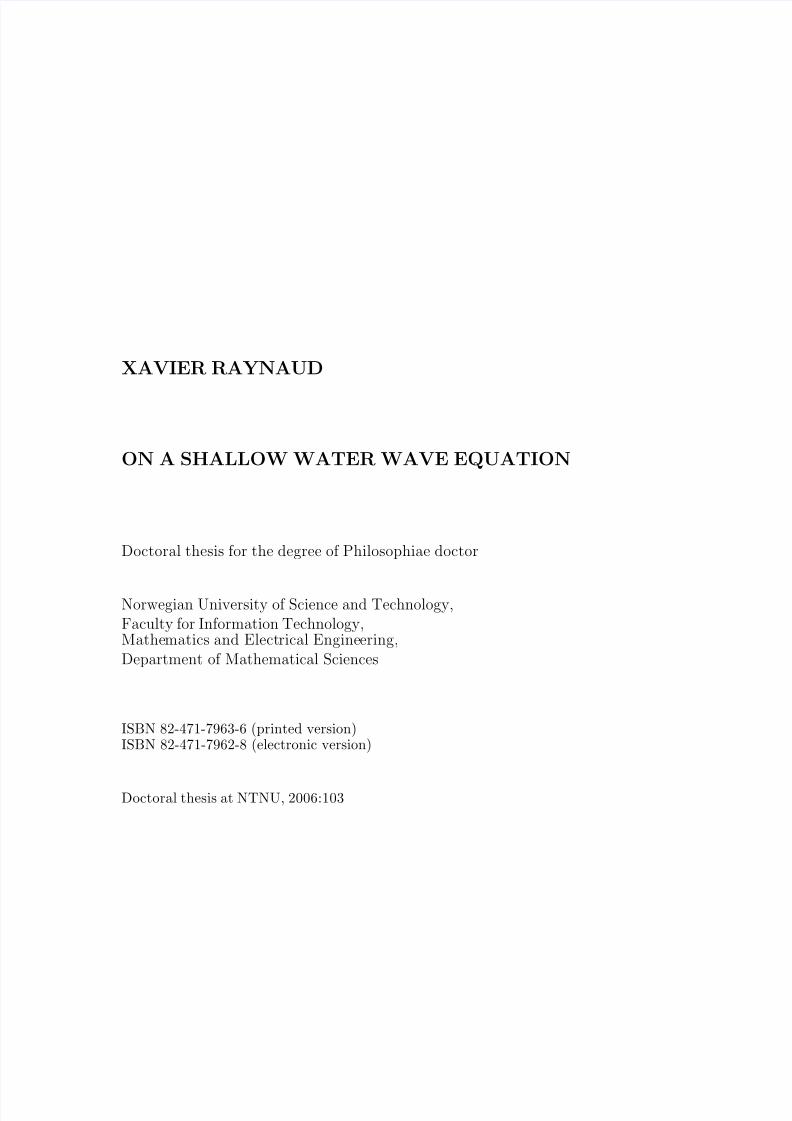
XAVIER RAYNAUD
ON A SHALLOW WATER WAVE EQUATION
Doctoral thesis for the degree of Philosophiae doctor
Norwegian University of Science and Technology,
Faculty for Information Technology,Mathematics and Electrical Engineering,
Department of Mathematical Sciences
ISBN 82-471-7963-6 (printed version)ISBN 82-471-7962-8 (electronic version)
Doctoral thesis at NTNU, 2006:103

8/3/2019 Xavier Raynaud- On a Shallow Water Wave Equation
http://slidepdf.com/reader/full/xavier-raynaud-on-a-shallow-water-wave-equation 2/161

8/3/2019 Xavier Raynaud- On a Shallow Water Wave Equation
http://slidepdf.com/reader/full/xavier-raynaud-on-a-shallow-water-wave-equation 3/161
To my parents,Pierre and Colette.

8/3/2019 Xavier Raynaud- On a Shallow Water Wave Equation
http://slidepdf.com/reader/full/xavier-raynaud-on-a-shallow-water-wave-equation 4/161
8/3/2019 Xavier Raynaud- On a Shallow Water Wave Equation
http://slidepdf.com/reader/full/xavier-raynaud-on-a-shallow-water-wave-equation 5/161
Acknowledgements
This thesis contains my research as a PhD student at the Department of Mathematical Sciences
at the Norwegian University of Sciences and Technology. My PhD was founded by the depart-
ment. The working and research conditions at the department are really excellent and gratefully
acknowledged.
First, I would like to thank my advisor, prof. Helge Holden. His genuine interest for this work
has been for me one of the most important sources of motivation. I am very grateful to him for
his constant support and for the many discussions we have had and that were so determinant
for this thesis.
I also would like to thank Henrik Kalisch for having suggested new problems and initiated an
interesting and fruitful collaboration.
As part of my PhD I spent four months in fall 2005 at the Mittag Leffler Institute in Djursholm,
Sweden. I am very grateful to the institute for the grant they gave me and for the wonderful
environment for research they provided.
Finally I would like to thank Mette. The last four years have been hectic – for both of us – but
they have also been happy years thanks to her and to our very lively little boy, Espen.

8/3/2019 Xavier Raynaud- On a Shallow Water Wave Equation
http://slidepdf.com/reader/full/xavier-raynaud-on-a-shallow-water-wave-equation 6/161
8/3/2019 Xavier Raynaud- On a Shallow Water Wave Equation
http://slidepdf.com/reader/full/xavier-raynaud-on-a-shallow-water-wave-equation 7/161
INTRODUCTION
The main topic of this thesis is the study of a nonlinear partial differential equation, theCamassa–Holm (CH) equation:
ut − utxx + 3uux − 2uxuxx − uuxxx = 0. (1)
The origin of the Camassa-Holm equation can by traced back to an article from Fuchssteinerand Fokas ([18]) from 1981 where it appears as one member of a whole family of bi-hamiltonianequations generated by the method of recursion operator. However some coefficients were notcorrectly computed. This may be the reason why no special attention was given to it until itsrediscovery in 1993 by Camassa and Holm in the context of water wave ([7, 8]). They derivedequation (1) as a model for unidirectional water wave propagation in shallow water with u
representing the height of the water’s free surface above a flat bottom. The relevance of theequation as a model for shallow water wave has been further investigated by Johnson in [21].
In 1998 a similar equation, namely
ut − utxx + 3uux − γ (2uxuxx + uuxxx) = 0, (2)
was discovered independently by Dai as a model for nonlinear waves in cylindrical axially sym-metric hyperelastic-rod. In this case, u(x, t) represents the radial stretch and γ a constantdepending on the property of the material.
a rich mathematical structure
The Camassa–Holm enjoys many remarkable mathematical properties. It is bi-Hamitonian,that is, it possesses two distinct but compatible hamiltonians. Following the methodology de-scribed in [24] for general bi-Hamiltonian systems, it is possible to derive an infinite number of conserved quantities for the solutions of (1); the computation is carried out in detail in [22]. Theequation admits a Lax-pair and is also formally integrable by means of scattering and inversescattering techniques. The scattering problem consists of computing the scattered far-field overan obstacle whose “shape” is determined in some way by u (for t fixed). In practice, it meansfinding the eigenvalues of a linear operator depending on u(t, x). The remarkable fact is thatas time evolves, if u(t, x) satisfies (1), then these eigenvalues satisfy trivial linear ordinary dif-ferential equations which can be solved explicitly and the far-field can be determined for anytime. The inverse scattering problem consists of retrieving the “shape” of the obstacle, that isu, from the knowledge of the scattered far-field. This is also a nontrivial but nevertheless linearproblem so that one can think of the scattering-inverse scattering method as a way of linearizing
the equation. If this approach can be (formally) followed then the system is (formally) integrableand solutions of the Camassa–Holm equation exist and can be computed. For a large class of initial data, it is indeed possible, see [10, 16].
It turns out that many physical relevant equations share the same structure (Lax pair, com-plete integrability via scattering and inverse scattering techniques), the paramount example beingthe KdV equation
ut + uux − uxxx = 0 (3)
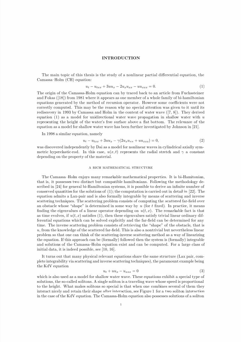
which is also used as a model for shallow water wave. These equations exhibit a special type of solutions, the so-called solitons. A single soliton is a traveling wave whose speed is proportionalto the height. What makes solitons so special is that when one combines several of them theyinteract nicely and retain their shape after interaction, see Figure 1 for a two soliton interactionin the case of the KdV equation. The Camassa-Holm equation also possesses solutions of a soliton
1
8/3/2019 Xavier Raynaud- On a Shallow Water Wave Equation
http://slidepdf.com/reader/full/xavier-raynaud-on-a-shallow-water-wave-equation 8/161
2 INTRODUCTION
−10 0 100
10
u
x
t = 0
−10 0 100
10
u
x
t = 0.3
−10 0 100
10
u
x
t = 0 .6
Figure 1. Interaction of two solitons for the KdV equation.
−20 0 300
2
u
x
t = 0
−20 0 300
2
u
x
t = 9.4
−20 0 300
2
u
x
t = 17
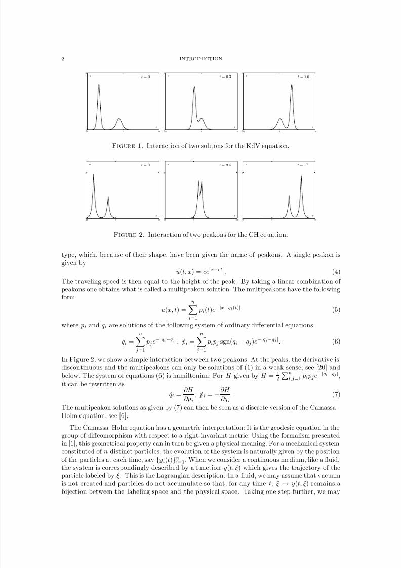
Figure 2. Interaction of two peakons for the CH equation.
type, which, because of their shape, have been given the name of peakons. A single peakon isgiven by
u(t, x) = ce|x−ct|. (4)
The traveling speed is then equal to the height of the peak. By taking a linear combination of peakons one obtains what is called a multipeakon solution. The multipeakons have the following
formu(x, t) =
ni=1
pi(t)e−|x−qi(t)| (5)
where pi and qi are solutions of the following system of ordinary differential equations
qi =n
j=1
pje−|qi−qj |, ˙ pi =n
j=1
pi pj sgn(qi − qj)e−|qi−qj |. (6)
In Figure 2, we show a simple interaction between two peakons. At the peaks, the derivative isdiscontinuous and the multipeakons can only be solutions of (1) in a weak sense, see [20] andbelow. The system of equations (6) is hamiltonian: For H given by H = 1
2
ni,j=1 pi pje−|qi−qj |,
it can be rewritten as
qi
=∂H
∂pi
, ˙ pi
= −∂H
∂qi. (7)
The multipeakon solutions as given by (7) can then be seen as a discrete version of the Camassa–Holm equation, see [6].
The Camassa–Holm equation has a geometric interpretation: It is the geodesic equation in thegroup of diffeomorphism with respect to a right-invariant metric. Using the formalism presentedin [1], this geometrical property can in turn be given a physical meaning. For a mechanical systemconstituted of n distinct particles, the evolution of the system is naturally given by the positionof the particles at each time, say {yi(t)}ni=1. When we consider a continuous medium, like a fluid,the system is correspondingly described by a function y(t, ξ) which gives the trajectory of theparticle labeled by ξ. This is the Lagrangian description. In a fluid, we may assume that vacuumis not created and particles do not accumulate so that, for any time t, ξ → y(t, ξ) remains abijection between the labeling space and the physical space. Taking one step further, we may
8/3/2019 Xavier Raynaud- On a Shallow Water Wave Equation
http://slidepdf.com/reader/full/xavier-raynaud-on-a-shallow-water-wave-equation 9/161
INTRODUCTION 3
as well assume that y(t, ·) remains a smooth diffeomorphism so that y : t → y(t, ·) can be seenas a path in the group of diffeomorphism from R
n to Rn (n is the dimension of the system).Formally, the group of smooth diffeomorphism, which we denote G, can be given the structure
of a Riemannian Lie group, the Riemannian metric then representing the energy of the system.The physically relevant path is then determined by the least action principle which says thaty : t → y(t, ·) is a geodesic in G. We consider a homogeneous fluid for which the particles areundistinguishable. In this case the initial labeling is arbitrary and, at each given time, it must bepossible to relabel the particles in a arbitrarily way without changing the evolution of the system.The evolution of the system depends only on the velocity distribution and the actual position of the particles should not matter as they are undistinguishable. A pure Eulerian description of thesystem is possible: Instead of looking at the trajectory of each individual particle, one consider,for a fixed point x in space, the velocity u(t, x) of the particle that at time t goes through x,that is,
u(t, x) = yt(t, y−1(t, x)).
The system enjoys what is called a relabeling symmetry . In the topological framework of Arnold
and Khesin, the relabeling symmetry corresponds to the fact that the metric of G is right-invariant. Then, by Noether’s theorem, one derives the existence of a conserved quantity holdingpoint-wise in space and which, by analogy with the rigid body problem, is called angular mo-
mentum . Furthermore, this framework provides a generic way of deriving the Euler equation forhydrodynamical systems. For the Camassa–Holm equation, the right-invariant metric is givenby
R
yt ◦ y−1
2+
∂ x(yt ◦ y−1)2
dx =
R
(u2 + u2x) dx
and the preservation of the angular momentum writes(u − uxx) ◦ y(t, ξ)
yξ(t, ξ)2 =
(u − uxx) ◦ y(0, ξ)
yξ(0, ξ)2 (8)
for all time and ξ ∈ R, see [13, 14, 15].
Local well-posedness and blow-up of the solutions
Local existence and well-posedness of solutions to (1) have been studied in [25, 11] with thehelp of Kato’s semi-group theory and in [23] using a regularization technique. It is shown that,for u0 ∈ H s(R) with s > 3
2, there exists a unique solution u with
u ∈ C ([0, T ), H s(R)) ∩ C 1([0, T ), H 1
2 (R))
where T > 0 only depends on u0H s(R). Solutions have to be understood in the weak sense or
in the sense of distribution. Equation (1) can be rewritten as
ut + uux + P x = 0, (9a)P − P xx = u2 +
1
2u2x. (9b)
The operator 1 − ∂ xx is a bijection from S into S where S denotes the class of tempereddistribution (see [19]) and a sufficient condition for (9) to hold in the sense of distribution is forexample that u ∈ L1
loc(R, H 1(R)).
These results hold only for a finite time interval and the CH equation, in contrast with theKdV equation, has smooth solutions that blow up in finite time. Due to their bi-hamiltonianstructure, the KdV and CH equations possess infinitely many conserved quantities. In the case of the KdV equation these quantities provide some apriori control on the regularity of the solutionand yield global existence and uniqueness of smooth solutions. However, this argument does notapply to the CH equation where only one such conserved quantity, the H 1(R) norm, can be used
8/3/2019 Xavier Raynaud- On a Shallow Water Wave Equation
http://slidepdf.com/reader/full/xavier-raynaud-on-a-shallow-water-wave-equation 10/161
4 INTRODUCTION
that way. The solution blows up in the following manner. Let T be the time where a smoothsolution eventually loses its regularity, i.e., limt→T u(t, ·)H s = ∞ for all s > 1. Then,
limt→T
inf x∈R
ux(t, x) = −∞. (10)
There appears a point where the profile of u steepens gradually and ultimately the slope becomesvertical. In the context of water waves, this corresponds to the breaking of a wave. This fact wasalready noted in the seminal papers of Camassa and Holm ([7, 8]) and was subsequently provedby Constantin and Escher ([11, 12]). Wave breaking is an important physical phenomenon whichis not captured by the other standard shallow water equations, as for example the KdV equation,and therefore makes the CH equation particularly interesting in that context.
The peakon and multipeakon as defined in (4) and (5) belong to H s(R) (for t fixed) only whens < 3
2and therefore are not included in the existence theorems mentioned above. The H 1(R)
norm is preserved by the equation, it plays a special role in the geometrical interpretation of theequation and H 1(R) can be seen as the natural space for the equation. These facts motivate theinvestigation of an H 1(R) theory for the CH equation.
Global existence of solutions
The first major step in this direction was accomplished by Constantin and Escher in [17].They prove that, for u0 ∈ H 1(R) and u0 − u0,xx ∈ M+(R), the space of positive Radon measure,equation (9) admit a unique global solution u in C 1(R, L2(R)) ∩ C (R, H 1(R)). They proceed asfollows. They consider a smooth approximation of the initial data, which for simplicity we alsodenote u0, satisfying the sign condition u0 − u0,xx ≥ 0 and the corresponding solution u givenby the local existence theory. Formally, it follows directly from (8) that
(u − uxx)(t, x) ≥ 0 (11)
for t ∈ [0, T ) and x ∈ R; a rigorous proof of (11) is given in [11]. The fact that the sign of
u − uxx is preserved leads to an apriori estimate for the total variation of ux as the followingsimple (formal) computation shows. We have
TV(ux) = uxxM(R) ≤ 2 uL1(R) , (12)
because uxxM(R) = R
|uxx| dx ≤ R
|u − uxx| dx + R
|u| dx = 2 R
|u| dx. Since the operator
(1−∂ xx)−1 preserves positivity, we have u ≥ 0 and R
|u| dx = R
u dx = R
u0 dx (we see directly
from (9a) that R
u dx is a conserved quantity). Therefore, TV(ux) ≤ 2 u0L1(R). This apriori
bound implies that ux remains bounded and the blow-up situation given by (10) cannot occur.There is no wave breaking and the solution exists globally in time. Moreover, it gives enoughcontrol on the approximated solutions to prove by compactness the existence of solutions inC (R, H 1(R)). In the two first papers, we present numerical schemes for the same class of initialdata based on a finite difference scheme (Paper I) and on multipeakons (Paper II). Both
schemes preserve the positivity of u − uxx. This is the key property that enables us to derive anapriori bound of the same type of (12) for our approximated solutions, and the convergence of the schemes is proved by a compactness argument.
In the case of arbitrary initial data in H 1(R), solutions are no longer unique. To illustratethis fact we look at the following multipeakon configuration where a peakon traveling from theleft to the right collides with another peakon going in the opposite direction (since this peakonhas its peak pointing downwards, it is called antipeakon), see Figure 3. In the antisymmetriccase, that is p1 = − p2 and q1 = −q2, the solution at collision time is identically zero. Then toprolong the solutions, two scenarios at least are possible. The first one consists of letting u remainidentically zero after collusion. It can be checked directly that this is indeed a weak solution of (9). The second scenario is provided by Beals, Sattinger and Szmigielski in [2, 3] where they deriveanalytical solutions for the multipeakons by using scattering and inverse scattering techniques.
8/3/2019 Xavier Raynaud- On a Shallow Water Wave Equation
http://slidepdf.com/reader/full/xavier-raynaud-on-a-shallow-water-wave-equation 11/161
INTRODUCTION 5
−20 0 20
0
u
x
t =−10
−20 0 20
0
u
x
t =−0 . 3
−20 0 20
0
u
x
t ≥0
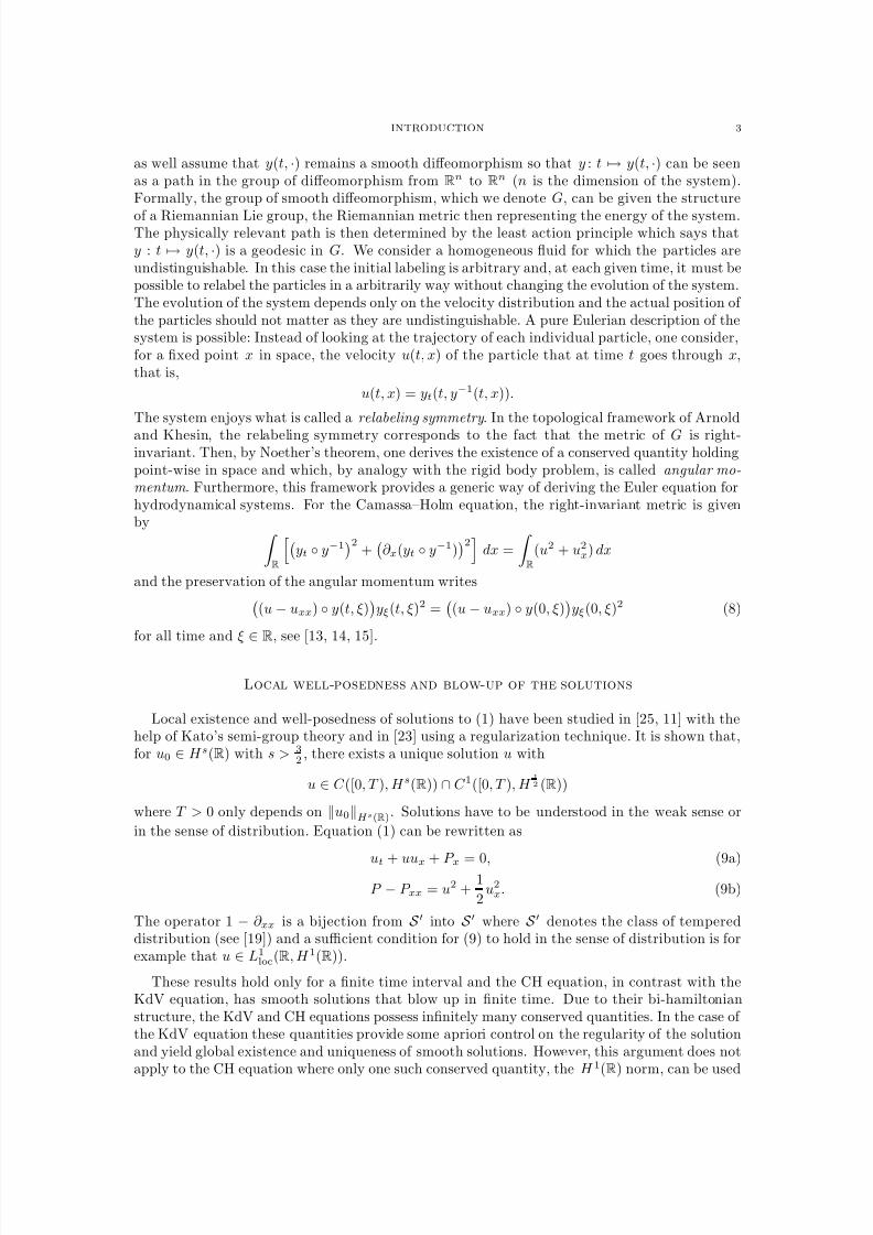
Figure 3. Peakon-antipeakon collision. First scenario: The dissipative solution.
−20 0 20
0
u
x
u
x
t =−10
t =−0 . 3
−20 0 20
0
u
x
t =0
−20 0 20
0
u
x
u
x
t =0 . 3
t =1 0
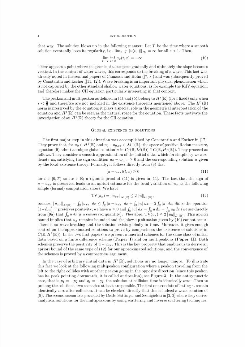
Figure 4. Peakon-antipeakon collision. Second scenario: The conservative solution.
For the solution they obtain in the antisymmetric peakon-antipeakon case, the peakons re-emergeafter the collision in such a way that the transformation t → −t, x → −x, which let equation(1) invariant, also lets the solution invariant (here we assume that t = 0 at collision), see Figure4. The solution is time reversible. Let E (t) = u(t, ·)H 1(R) denote the energy of the system.
In the time reversible case illustrated in Figure 4, for any t different from collision time (t = 0),
E (t) remains equal to the same strictly positive constant, say E (t) = 1, while at collision time,we have E (0) = 0. In the other case illustrated in Figure 3 we have E (t) = 1 for t < 0 andE (t) = 0 for t ≥ 0. One can prolong the solution after collision in infinitely many ways but thetwo scenarios we mentioned are really the only reasonable ones and the question is how they canbe characterized and what is the selection principle that can be used to capture each of them.
By using viscous approximations of the equation, Xin and Zhang in [26] obtain the existenceof a solution u ∈ C ([0, ∞) ×R
1) ∩ L∞((0, ∞), H 1(R)) to the CH equation for any initial data inu0 ∈ H 1(R). In particular their solution satisfies
E (t) = u(t, ·)H 1(R) ≤ E (t) = u(t, ·)H 1(R) (13)
for all t < t and the following one-sided super-norm estimate on ux holds
ux(
t, x) ≤
1
t +C, t >
0, x
∈R.
(14)Because of (13), we call these solutions dissipative solutions: the energy can only decay. In [9]it is proven that dissipative solutions are unique. In the symmetric peakon-antipeakon case, itis clear that the dissipative solution is the one corresponding to Figure 3.
In [4], Bressan and Constantin introduce a new set of variable,
w = u(t, y), v = 2 arctanux, q = (1 + u2x)yξ (15)
where y(t, ξ) denotes the characteristics, i.e., yt(t, ξ) = u(t, y(t, ξ)). They rewrite equation (1)uniquely in terms of these new variables and the system of equations they obtain, turns out tobe a well-posed system of ordinary differential equation in a Banach space. Well-posed ordi-nary differential equation are time reversible and indeed this change of variable selects the timereversible solution in the antisymmetric peakon-antipeakon problem, which is given in Figure
8/3/2019 Xavier Raynaud- On a Shallow Water Wave Equation
http://slidepdf.com/reader/full/xavier-raynaud-on-a-shallow-water-wave-equation 12/161
6 INTRODUCTION
00
u2 +u
2
x
x
t =−1 . 8
t =−0 . 8
t =−0 . 3
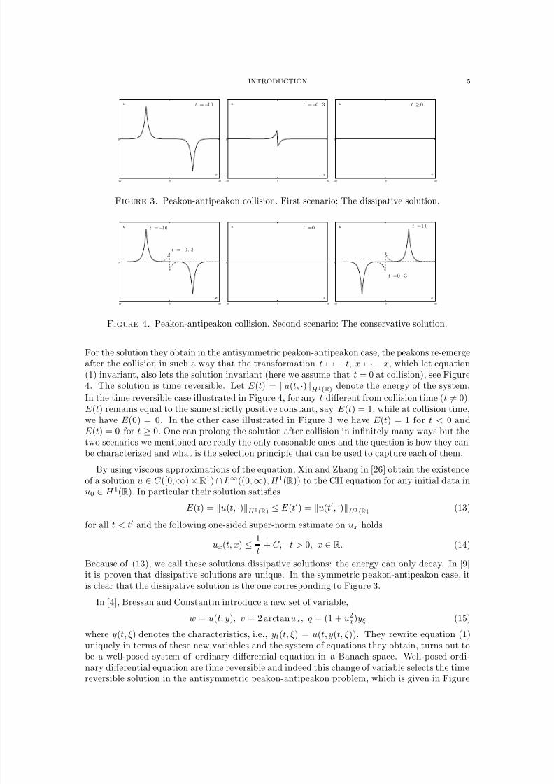
Figure 5. The energy density in the peakon-antipeakon case
4. The approach adopted in [5] by Bressan and Fonte is substantially different. They start byconsidering a system of multipeakons and describe the dynamic of the system, in particular howthe multipeakons evolve throughout the collisions. At this stage, they select the conservativesolution. Then, they introduce a distance functional inspired by optimal transport theory whichsatisfies
d
dtJ (u(t), v(t)) ≤ κJ (u(t), v(t)) (16)
for any conservative multipeakons solutions u and v. Identity (16) is precisely the one neededto use Gronwall’s Lemma and obtain stability results. General solutions to the CH equation arefinally constructed from the multipeakons by a density argument.
Our approach in Paper IV is similar to the one of Bressan and Constantin. We reformulatethe equation by using a new set of variables. The variables (y,U ,H ) we use have a natural
interpretation from the Lagrangian point of view. As before, y denotes the characteristics andis given by
yt(t, ξ) = u(t, y(t, ξ)) (17)
while
U (t, ξ) = u(t, y(t, ξ)) and H (t, ξ) =
y(t,ξ)
−∞
(u2(t, x) + u2x(t, x)) dx (18)
correspond to the Lagrangian velocity and the cumulative energy distribution, respectively.Equation (9) can be rewritten as a system of ordinary differential equation in a Banach spaceinvolving uniquely (y,U ,H ). The system is well-posed and we obtain the global existence of solution.
The original equation (1) which corresponds to the Euler formulation of the problem containsonly one unknown function, the velocity field u. The Lagrangian description as we introduced it inthe first section contains two unknown functions: the position and the velocity of the particles,y and U . In order to explain why the extra variable H describing the energy distribution isneeded, we look again at the peakon-antipeakon problem. At collision time, say t = 0, u isidentically zero. Since zero is a global solution of (1), it is necessary, in order to select theconservative solution after collision, to take into account what happened before collision, to keeptrack in some way of the history of the system. The H 1(R) norm of u is a preserved quantityand
R
u2(t, x) + u2
x(t, x)
dx remains equal to a constant, say 1, up to collision. In Figure 5,
we plot the function u2(t, x) + u2x(t, x) at different times. As it can also be seen from Figure 4,
limt→0 u(t, ·)L∞(R) = 0 and limt→0
supx∈R\[q1,q2] |ux(t, x)|
= 0 so that all the mass of u2 +u2
x
concentrates at the origin. We have
limt→0
(u2(t, x) + u2x(t, x)) dx = δ(x)
8/3/2019 Xavier Raynaud- On a Shallow Water Wave Equation
http://slidepdf.com/reader/full/xavier-raynaud-on-a-shallow-water-wave-equation 13/161
INTRODUCTION 7
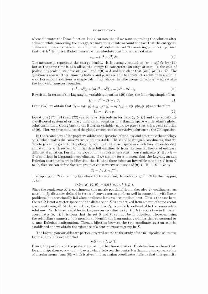
where δ denotes the Dirac function. It is clear now that if we want to prolong the solution aftercollision while conserving the energy, we have to take into account the fact that the energy atcollision time is concentrated at one point. We define the set D consisting of pairs (u, µ) such
that u ∈ H 1(R), µ is a Radon measure whose absolute continuous part satisfiesµac = (u2 + u2
x) dx. (19)
The measure µ represents the energy density. It is strongly related to (u2 + u2x) dx by (19)
but at the same time it also allows the energy to concentrate on singular sets. In the case of peakon-antipeakon, we have u(0) = 0 and µ(0) = δ and it is clear that (u(0), µ(0)) ∈ D. Thequestion is now whether, knowing both u and µ, we are able to construct a solution in a uniqueway. For smooth solutions, a simple calculation shows that the energy density u2 + u2
x satisfiesthe following transport equation
(u2 + u2x)t + (u(u2 + u2
x))x = (u3 − 2P u)x. (20)
Rewritten in terms of the Lagrangian variables, equation (20) takes the following simpler form
H t = U 3 − 2P ◦ y U. (21)
From (9a), we obtain that U t = ut(t, y) + ytux(t, y) = ut(t, y) + u(t, y)ux(t, y) and therefore
U t = −P x ◦ y. (22)
Equations (17), (21) and (22) can be rewritten only in terms of (y,U ,H ) and they constitutea well-posed system of ordinary differential equation in a Banach space which admits globalsolutions in time. Going back to the Eulerian variable (u, µ), we prove that u is a weak solutionof (9). Thus we have established the global existence of conservative solutions to the CH equation.
In the second part of the paper we address the question of stability and determine the topologyon D which makes the conservative solutions stable. The set of Lagrangian coordinates, that wedenote G, can be given the topology induced by the Banach space in which they are embeddedand stability with respect to initial data follows directly from the general theory of ordinarydifferential equation. Furthermore, we obtain the existence a continuous semigroup S : R
+× G →
G of solutions in Lagrangian coordinates. If we assume for a moment that the Lagrangian andEulerian coordinates are in bijection, that is, that there exists an invertible mapping f from Gto D, then we can define the semigroup of conservative solutions of (9) T : R+ × D → D by
T t = f ◦ S t ◦ f −1.
The topology on D can simply be defined by transporting the metric on G into D by the mappingf , i.e.,
dD((u, µ), (u, µ)) = dG(f (u, µ), f (u, µ)).
Since the semigroup S t is continuous, this metric per definition makes also T t continuous. Asnoted in [5], distances defined in terms of convex norms perform well in connection with linearproblems, but occasionally fail when nonlinear features become dominant. This is the case here,the set D is not a vector space and the distance on D is not derived from a norm of some vector
space containing D. At the same time, the metric dD is perfectly well-suited to the conservativesolutions. With three variables in Lagrangian coordinates (y, U , H ) versus two in Euleriancoordinates (u, µ), it is clear that the set G and D can not be in bijection. However, usingthe relabeling symmetry, it is possible to identify the Lagrangian variables that correspond toa same Eulerian configuration. Then, a bijection between the two coordinates systems can beestablished and we obtain the existence of a continuous semigroup in D.
The Lagrangian variables are particularly well-suited to the study of the multipeakon solutions.From (5) and (6) we infer that
qi(t) = u(t, qi(t)).
Hence, the positions of the peaks are given by the characteristics. By definition, we have that,for a multipeakon u, u − uxx = 0 everywhere between the peaks. Furthermore the conservationof angular momentum (8), which is given in Lagrangian coordinates, tells us that this quantity
8/3/2019 Xavier Raynaud- On a Shallow Water Wave Equation
http://slidepdf.com/reader/full/xavier-raynaud-on-a-shallow-water-wave-equation 14/161
8 INTRODUCTION
remains zero. In Paper V, we prove that the conservative solutions preserve the multipeakonstructure, i.e., multipeakons are conservative solutions in the sense defined in Paper IV. More-over, we derive a system of ordinary differential equation, globally defined, for the conservative
multipeakon solutions.
The Lagrangian approach is sufficiently robust to handle a larger class of equation. In Paper
VI, we prove the existence of a global continuous semigroup of conservative solutions for
ut − uxxt + f (u)x − f (u)xxx + (g(u) +1
2f (u)(ux)2)x = 0 (23)
with f ∈ W 3,∞
loc (R), f strictly convex or concave, g ∈ W 1,∞
loc (R). For f (u) = u2
2 and g(u) =
κu + u2, (23) gives the Camassa–Holm equation while, for f (u) = γu2
2 and g(u) = 3−γ2
u2, it givesthe hyperelastic rod equation (2).
In Paper III we look at the smooth-solutions of (1) in contrast with the other papers wherethe focus was set on solutions with low spatial regularity. We prove the spectral convergence of
the Fourier-Galerkin and a de-aliased Fourier-collocation for the Camassa–Holm equation.
References
[1] V. I. Arnold and B. A. Khesin. Topological methods in hydrodynamics, volume 125 of Applied Mathematical Sciences. Springer-Verlag, New York, 1998.
[2] R. Beals, D. H. Sattinger, and J. Szmigielski. Multi-peakons and a theorem of Stieltjes. Inverse Problems,15(1):L1–L4, 1999.
[3] R. Beals, D. H. Sattinger, and J. Szmigielski. Multipeakons and the classical moment problem. Adv. Math.,154(2):229–257, 2000.
[4] A. Bressan and A. Constantin. Global conservative solutions of the Camassa–Holm equation. Preprint, Sub-mitted , 2005.
[5] A. Bressan and M. Fonte. An optimal transportation metric for solutions of the Camassa–Holm equation.Preprint, Submitted , 2005.
[6] R. Camassa. Characteristics and the initial value problem of a completely integrable shallow water equation.Discrete Contin. Dyn. Syst. Ser. B , 3(1):115–139, 2003.
[7] R. Camassa and D. D. Holm. An integrable shallow water equation with peaked solitons. Phys. Rev. Lett.,71(11):1661–1664, 1993.
[8] R. Camassa, D. D. Holm, and J. Hyman. A new integrable shallow water equation. Adv. Appl. Mech., 31:1–33,1994.
[9] G. M. Coclite, H. Holden, and K. H. Karlsen. Global weak solutions to a generalized hyperelastic-rod waveequation. SIAM J. Math. Anal., 37(4):1044–1069 (electronic), 2005.
[10] A. Constantin. On the scattering problem for the Camassa-Holm equation. R. Soc. Lond. Proc. Ser. A Math.Phys. Eng. Sci., 457(2008):953–970, 2001.
[11] A. Constantin and J. Escher. Global existence and blow-up for a shallow water equation. Ann. Scuola Norm.Sup. Pisa Cl. Sci. (4), 26(2):303–328, 1998.
[12] A. Constantin and J. Escher. Wave breaking for nonlinear nonlocal shallow water equations. Acta Math.,181(2):229–243, 1998.
[13] A. Constantin and B. Kolev. Least action principle for an integrable shallow water equation. J. Nonlinear
Math. Phys., 8(4):471–474, 2001.[14] A. Constantin and B. Kolev. On the geometric approach to the motion of inertial mechanical systems. J.
Phys. A, 35(32):R51–R79, 2002.[15] A. Constantin and B. Kolev. Geodesic flow on the diffeomorphism group of the circle. Comment. Math. Helv.,
78(4):787–804, 2003.[16] A. Constantin and J. Lenells. On the inverse scattering approach to the Camassa-Holm equation. J. Nonlinear
Math. Phys., 10(3):252–255, 2003.[17] A. Constantin and L. Molinet. Global weak solutions for a shallow water equation. Comm. Math. Phys.,
211(1):45–61, 2000.[18] B. Fuchssteiner and A. S. Fokas. Symplectic structures, their Backlund transformations and hereditary sym-
metries. Phys. D, 4(1):47–66, 1981/82.[19] H. Holden and X. Raynaud. Convergence of a finite difference scheme for the camassa–holm equation. SIAM
J. Numer. Anal. 2006 , to appear. paper I in this thesis.[20] H. Holden and X. Raynaud. A convergent numerical scheme for the camassa–holm equation based on multi-
peakons. Discrete Contin. Dyn. Syst., 14(3), 2006. paper II in this thesis.
8/3/2019 Xavier Raynaud- On a Shallow Water Wave Equation
http://slidepdf.com/reader/full/xavier-raynaud-on-a-shallow-water-wave-equation 15/161
INTRODUCTION 9
[21] R. S. Johnson. Camassa–Holm, Korteweg-de Vries and related models for water waves. J. Fluid Mech.,455:63–82, 2002.
[22] J. Lenells. Conservation laws of the Camassa-Holm equation. J. Phys. A, 38(4):869–880, 2005.[23] Y. A. Li and P. J. Olver. Well-posedness and blow-up solutions for an integrable nonlinearly dispersive model
wave equation. J. Differential Equations, 162(1):27–63, 2000.[24] P. J. Olver. Applications of Lie groups to differential equations, volume 107 of Graduate Texts in Mathemat-
ics. Springer-Verlag, New York, second edition, 1993.[25] G. Rodrıguez-Blanco. On the Cauchy problem for the Camassa-Holm equation. Nonlinear Anal., 46(3, Ser.
A: Theory Methods):309–327, 2001.[26] Z. Xin and P. Zhang. On the weak solutions to a shallow water equation. Comm. Pure Appl. Math.,
53(11):1411–1433, 2000.

8/3/2019 Xavier Raynaud- On a Shallow Water Wave Equation
http://slidepdf.com/reader/full/xavier-raynaud-on-a-shallow-water-wave-equation 16/161
8/3/2019 Xavier Raynaud- On a Shallow Water Wave Equation
http://slidepdf.com/reader/full/xavier-raynaud-on-a-shallow-water-wave-equation 17/161
Paper I
Convergence of a finite different schemefor the Camassa-Holm equation.
H. Holden and X. RaynaudTo appear in SIAM J. Numer. Anal.

8/3/2019 Xavier Raynaud- On a Shallow Water Wave Equation
http://slidepdf.com/reader/full/xavier-raynaud-on-a-shallow-water-wave-equation 18/161
8/3/2019 Xavier Raynaud- On a Shallow Water Wave Equation
http://slidepdf.com/reader/full/xavier-raynaud-on-a-shallow-water-wave-equation 19/161
CONVERGENCE OF A FINITE DIFFERENCE SCHEME FOR THECAMASSA–HOLM EQUATION
HELGE HOLDEN AND XAVIER RAYNAUD
Abstract. We prove that a certain finite difference scheme converges to the weak solution of the Cauchy problem on a finite interval with periodic boundary conditions for the Camassa–Holm equation ut−uxxt+3uux−2uxuxx−uuxxx = 0 with initial data u|t=0 = u0 ∈ H 1([0, 1]).Here it is assumed that u0 − u
0≥ 0 and in this case, the solution is unique, globally defined,
and energy preserving.
1. Introduction
The Camassa–Holm equation (CH) [3]
ut − uxxt + 2κux + 3uux − 2uxuxx − uuxxx = 0 (1.1)
has received considerable attention the last decade. With κ positive it models, see [4, 16, 12],propagation of unidirectional gravitational waves in a shallow water approximation, with u rep-resenting the fluid velocity. The Camassa–Holm equation possesses many intriguing properties:It is, for instance, completely integrable and experiences wave breaking in finite time for a largeclass of initial data. Most attention has been given to the case with κ = 0 on the full line, thatis,
ut − uxxt + 3uux − 2uxuxx − uuxxx = 0, (1.2)
which has so-called peakon solutions, i.e., solutions of the form u(x, t) = ce−|x−ct| for realconstants c. Local and global well-posedness results as well as results concerning breakdown areproved in [9, 14, 17, 20].
In this paper we study the Camassa–Holm equation (1.1) on a finite interval with periodicboundary conditions. It is known that certain initial data give global solutions, while otherclasses of initial data experience wave breaking in the sense that ux becomes unbounded whilethe solution itself remains bounded. It suffices to treat the case κ = 0, since solutions withnonzero κ are obtained from solutions with zero κ by the transformation v(x, t) = u(x+κt,t)−κ.More precisely, the fundamental existence theorem, due to Constantin and Escher [10], reads asfollows: If u0 ∈ H 3([0, 1]) and m0 := u0 − u0 ∈ H 1([0, 1]) is non-negative, then equation (1.2)has a unique global solution u ∈ C ([0, T ), H 3([0, 1])) ∩ C 1([0, T ), H 2([0, 1])) for any T positive.However, if m0 ∈ H 1([0, 1]), u0 not identically zero but
m0 dx = 0, then the maximal time
interval of existence is finite. Furthermore, if u0
∈H 1([0, 1]) and m0 = u0
−u0 is a positive
Radon measure on [0, 1], then (1.2) has a unique global weak solution. Additional results in theperiodic case can be found in [7, 10, 8, 11, 18]. Numerical results can be found in [4] whereCamassa, Holm, and Hyman study (1.2) using a pseudospectral method. Numerical schemesbased on multipeakons are examined in [2, 6, 5, 15].
In this paper, we prove convergence of a particular finite difference scheme for the equation,thereby giving a constructive approach to the actual determination of the solution). We workin the case where one has global solutions, that is, when m0 ≥ 0. The scheme is semi-discrete:Time is not discretized, and we have to solve a system of ordinary differential equations. Wereformulate (1.1) to give meaning in C ([0, T ]; H 1[0, 1]) to solutions such as peakons, and we provethat our scheme converges in C ([0, T ]; H 1[0, 1]).
1991 Mathematics Subject Classification. Primary: 65M06, 65M12; Secondary: 35B10, 35Q53.Key words and phrases. Camassa–Holm equation, convergence of finite difference schemes.
1
8/3/2019 Xavier Raynaud- On a Shallow Water Wave Equation
http://slidepdf.com/reader/full/xavier-raynaud-on-a-shallow-water-wave-equation 20/161
2 H. HOLDEN AND X. RAYNAUD
More precisely, we prove the following: Assume that vn is a sequence of continuous, periodicand piecewise linear functions on intervals [(i − 1)/n, i/n], i = 1, . . . , n, that converges to theinitial data v in H 1([0, 1]) as n
→ ∞. Let un = un(x, t) be the solution of the following system
of equations
mnt = −D−(mnun) − mnDun
mn = un − D−D+un(1.3)
with initial condition un|t=0 = vn. Here D± denotes forward and backward difference operatorsrelative to the lattice with spacing 1/n, and D = (D+ + D−)/2. Extrapolate un from its latticevalues at points i/n to obtain a continuous, periodic, and piecewise linear function also denotedun. Assume that vn − D−D+vn ≥ 0. Then un converges in C ([0, T ]; H 1([0, 1])) as n → ∞ to thesolution u of the Camassa–Holm equation with initial condition u|t=0 = v. The result includesthe case when the initial data v ∈ H 1 is such that v − vxx is a positive Radon measure, seeCorollary 2.5. For the actual computations we discretize (1.3) using the forward Euler method.We prove convergence of that method, see Theorem 3.1.
The numerical scheme (1.3) is tested on various initial data. In addition, we study exper-imentally the convergence of other numerical schemes for the Camassa–Holm equation. Thenumerical results are surprisingly sensitive in the explicit form of the scheme, and, among thevarious schemes we have implemented, only the scheme (1.3) converges to the unique solution.
2. Convergence of the numerical scheme
We consider periodic boundary conditions and solve the equation on the interval [0 , 1]. Weare looking for solutions that belong to H 1([0, 1]) which is the natural space for the equation.Introduce the partition of [0, 1] in points separated by a distance h = 1/n denoted xi = hi fori = 0, . . . , n − 1. For any (u0, . . . , un−1) in Rn, we can define a continuous, periodic, piecewise
linear function u byu(xi) = ui, (2.1)
in other words, the periodic polygon that passes through the points (xi, ui) for i = 0, . . . , n − 1.It defines a bijection between Rn and the set of continuous, periodic, piecewise linear functionwith possible break points at xi, and we will use this bijection throughout this paper.
Given u = (u0, . . . , un−1), the quantity D±u given by
(D±u)i =±1
h(ui±1 − ui)
gives the right and left derivatives, respectively, of u at xi. In these expressions, u−1 and un arederived from the periodicity conditions: u−1 = un−1 and un = u0. The average Du between the
left and right derivative is given by
(Du)i =1
2
(D+u)i + (D−u)i
=
1
2h(ui+1 − ui−1).
The Camassa–Holm equation preserves the H 1-norm. In order to see that, we rewrite (1.2)in its Hamiltonian form, see [3]
mt = −(mu)x − mux (2.2)
with
m = u − uxx. (2.3)
8/3/2019 Xavier Raynaud- On a Shallow Water Wave Equation
http://slidepdf.com/reader/full/xavier-raynaud-on-a-shallow-water-wave-equation 21/161
FINITE DIFFERENCE SCHEME FOR THE CAMASSA–HOLM EQUATION 3
Assuming that u is smooth enough so that the integration by parts can be carried out, we get
d
dtu2
H 1 = 2 1
0
(ut − uxxt)u dx = 2 1
0
umt dx
= −2
1
0
u(mu)x dx − 2
1
0
umux dx
= 2
1
0
uxmudx − 2
1
0
umux dx = 0,
and the H 1 norm of u is preserved.From (2.3) and (2.2), we derive a finite difference approximation scheme for the Camassa–
Holm equation, and prove that it converges to the right solution. This is our main result.
Theorem 2.1. Let vn be a sequence of continuous, periodic and piecewise linear functions on [0, 1] that converges to v in H 1([0, 1]) as n → ∞ and such that vn−D−D+vn ≥ 0. Then, for any given T > 0, the sequence un = un(x, t) of continuous, periodic and piecewise linear functions
determined by the system of ordinary differential equationsmnt = −D−(mnun) − mnDun
mn = un − D−D+un(2.4)
with initial condition un|t=0 = vn, converges in C ([0, T ]; H 1([0, 1])) as n → ∞ to the solution uof the Camassa–Holm equation (1.2) with initial condition u|t=0 = v.
If we interpret the functions as vectors in (2.4), cf. (2.1), the multiplications are term-by-termmultiplications of vectors. We also have to rewrite equation (1.2) in order to make it well-defined in the sense of distributions for functions that at least belong to C ([0, T ]; H 1([0, 1])),more precisely,
ut − uxxt = − 3
2(u2)x − 1
2(u2
x)x +1
2(u2)xxx. (2.5)
A function u in L∞
([0, T ]; H 1
) is said to be solution of the periodic Camassa–Holm equation if itis periodic and satisfies (2.5) in the sense of distributions. In [11], a different definition of weaksolutions for the Camassa–Holm equation is presented. After proving our main theorem at theend of this section, we also prove that these two definitions are equivalent.
In order to solve equation (2.4), we need to compute un from mn. It is simpler first to considersequences that are defined in RZ, the set of all sequences, and then discuss the periodic case. LetL denote the linear operator from R
Z to RZ given, for all u ∈ RZ, by
Lu = u − D−D+u.
We want to find an expression for L−1. Introduce the Kronecker delta by δi = 1 if i = 0 andzero otherwise. It is enough to find a solution g of
Lg = δ
which decays sufficently fast at infinity because L−1m is then given, for any bounded m ∈ RZ
,by the discrete convolution product of g and m:
L−1mi =j∈Z
gi−jmj.
The function g satisfies for i nonzero
gi − n2(gi+1 − 2gi + gi−1) = 0. (2.6)
The general solution of (2.6) for all i ∈ Z is given by
gi = Aeκ1i + Beκ2i
where A, B are constants, κ1 = ln x1, κ2 = ln x2, and x1 and x2 are the solutions of
−n2x2 + (1 + 2n2)x
−n2 = 0.
8/3/2019 Xavier Raynaud- On a Shallow Water Wave Equation
http://slidepdf.com/reader/full/xavier-raynaud-on-a-shallow-water-wave-equation 22/161
4 H. HOLDEN AND X. RAYNAUD
Here x1 and x2 are real and positive, and x1x2 = 1 implies that κ2 = −κ1. We set κ = κ1 = −κ2.After some calculations, we get
κ = ln1 + 2n2 +√
1 + 4n2
2n2 . (2.7)
We take g of the form
gi = c e−κ|i|
so that g satisfies (2.6) for all i = 0 and decays at infinity. The constant c is determined by thecondition that (Lg)0 = 1 which yields
c =1
1 + 2n2(1 − e−κ).
We periodize g in the following manner:
g pi ≡ k∈Z gi+kn = ce−κi + eκ(i−n)
1−
e−κn
for i ∈ {0, . . . , n − 1}. The inverse of L on the set of periodic sequences is then given by
ui = L−1mi =
n−1j=0
g pi−jmi =c
1 − e−κn
n−1j=0
(e−κ(i−j) + eκ(i−j−n))mj . (2.8)
Hence,
L n−1j=0
g pi−jmj
i
= Ll∈Z
gi−lml
i
= mi.
For sufficiently smooth initial data (u0 ∈ H 3 and m0 ∈ H 1) which satisfies m0 ≥ 0, Constantinand Escher [9] proved that there exists a unique global solution of the Camassa–Holm equationbelonging to C (R+; H 3)
∩C 1(R+; H 2). The proof of this result relies heavily on the fact that if m
is non-negative at t = 0, then m remains non-negative for all t > 0. An important feature of ourscheme is that it preserves this property. (For simplicity we have here dropped the superscriptn appearing on u and m.)
Lemma 2.2. Assume that mi(0) ≥ 0 for all i = 0, . . . , n−1. For any solution u(t) of the system (2.4), we have that mi(t) ≥ 0 for all t ≥ 0 and for all i = 0, . . . , n − 1.
Proof. Let us assume that there exist t > 0 and i ∈ {0, . . . , n − 1} such that
mi(t) < 0. (2.9)
We consider the time interval F in which m remains positive:
F = {t ≥ 0 | mi(t) ≥ 0, for all t ≤ t and i ∈ {0, . . . , n − 1}}.
Because of assumption (2.9), F is bounded and we define
T = sup F.
By definition of T , for any integer j > 0, there exists a tj and an ij such that T < tj < T + 1j
and mij (tj) < 0. The function mij (t) is a continuously differentiable function of t. Hence,mij (T ) ≥ 0 and there exists a tj such that
mij (tj) = 0,
with T ≤ tj < T + 1j
.
Since ij can only take a finite number of values (ij ∈ {0, . . . , n − 1}), there exists a p ∈{0, . . . , n − 1} and a subsequence jk such that ijk = p. The function m p(t) belongs to C 1 and,since tjk → T , we have
m p(T ) = 0. (2.10)
8/3/2019 Xavier Raynaud- On a Shallow Water Wave Equation
http://slidepdf.com/reader/full/xavier-raynaud-on-a-shallow-water-wave-equation 23/161
FINITE DIFFERENCE SCHEME FOR THE CAMASSA–HOLM EQUATION 5
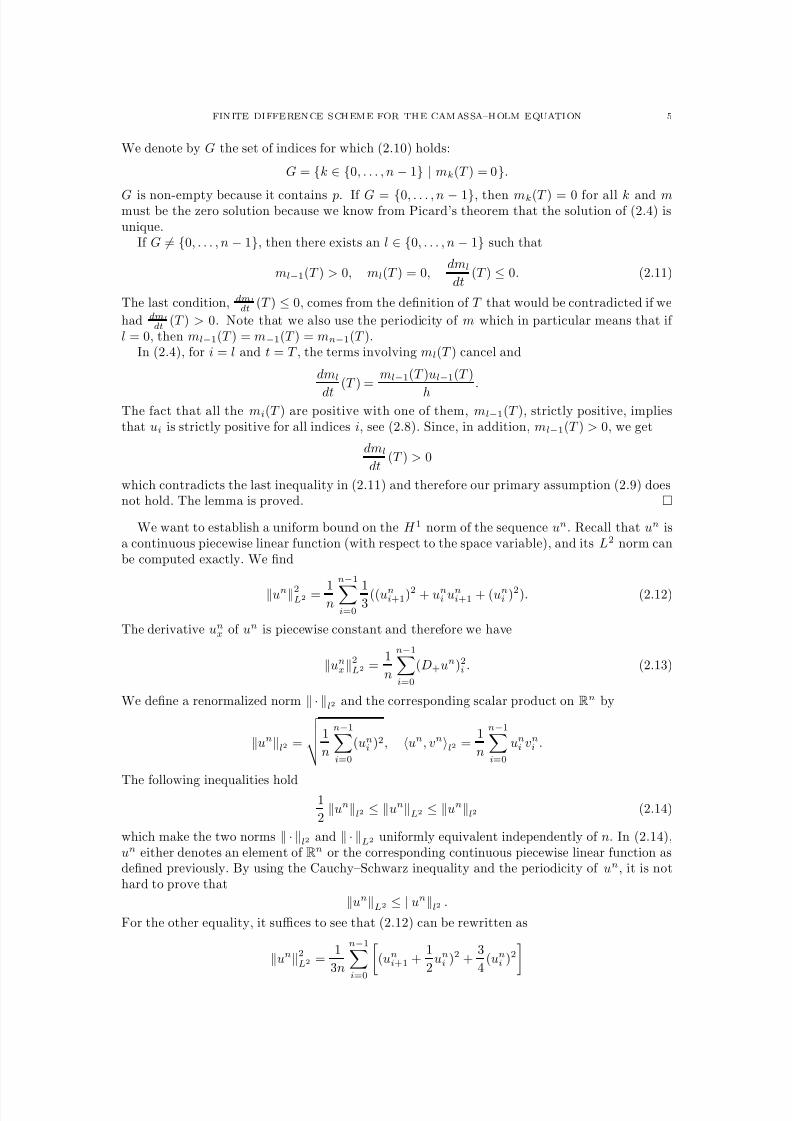
We denote by G the set of indices for which (2.10) holds:
G = {k ∈ {0, . . . , n − 1} | mk(T ) = 0}.
G is non-empty because it contains p. If G = {0, . . . , n − 1}, then mk(T ) = 0 for all k and mmust be the zero solution because we know from Picard’s theorem that the solution of (2.4) isunique.
If G = {0, . . . , n − 1}, then there exists an l ∈ {0, . . . , n − 1} such that
ml−1(T ) > 0, ml(T ) = 0,dml
dt(T ) ≤ 0. (2.11)
The last condition, dml
dt(T ) ≤ 0, comes from the definition of T that would be contradicted if we
had dml
dt(T ) > 0. Note that we also use the periodicity of m which in particular means that if
l = 0, then ml−1(T ) = m−1(T ) = mn−1(T ).In (2.4), for i = l and t = T , the terms involving ml(T ) cancel and
dml
dt(T ) =
ml−1(T )ul−1(T )
h.
The fact that all the mi(T ) are positive with one of them, ml−1(T ), strictly positive, impliesthat ui is strictly positive for all indices i, see (2.8). Since, in addition, ml−1(T ) > 0, we get
dml
dt(T ) > 0
which contradicts the last inequality in (2.11) and therefore our primary assumption (2.9) doesnot hold. The lemma is proved.
We want to establish a uniform bound on the H 1 norm of the sequence un. Recall that un isa continuous piecewise linear function (with respect to the space variable), and its L2 norm canbe computed exactly. We find
un2L2 = 1
n
n−1i=0
13
((uni+1)2 + uni uni+1 + (uni )2). (2.12)
The derivative unx of un is piecewise constant and therefore we have
unx2L2 =
1
n
n−1i=0
(D+un)2i . (2.13)
We define a renormalized norm · l2 and the corresponding scalar product on Rn by
unl2 =
1
n
n−1i=0
(uni )2, un, vnl2 =1
n
n−1i=0
uni vni .
The following inequalities hold1
2unl2 ≤ unL2 ≤ unl2 (2.14)
which make the two norms · l2 and · L2 uniformly equivalent independently of n. In (2.14),un either denotes an element of Rn or the corresponding continuous piecewise linear function asdefined previously. By using the Cauchy–Schwarz inequality and the periodicity of un, it is nothard to prove that
unL2 ≤ unl2 .
For the other equality, it suffices to see that (2.12) can be rewritten as
un2L2 =
1
3n
n−1
i=0 (uni+1 +
1
2uni )2 +
3
4(uni )2
8/3/2019 Xavier Raynaud- On a Shallow Water Wave Equation
http://slidepdf.com/reader/full/xavier-raynaud-on-a-shallow-water-wave-equation 24/161
8/3/2019 Xavier Raynaud- On a Shallow Water Wave Equation
http://slidepdf.com/reader/full/xavier-raynaud-on-a-shallow-water-wave-equation 25/161
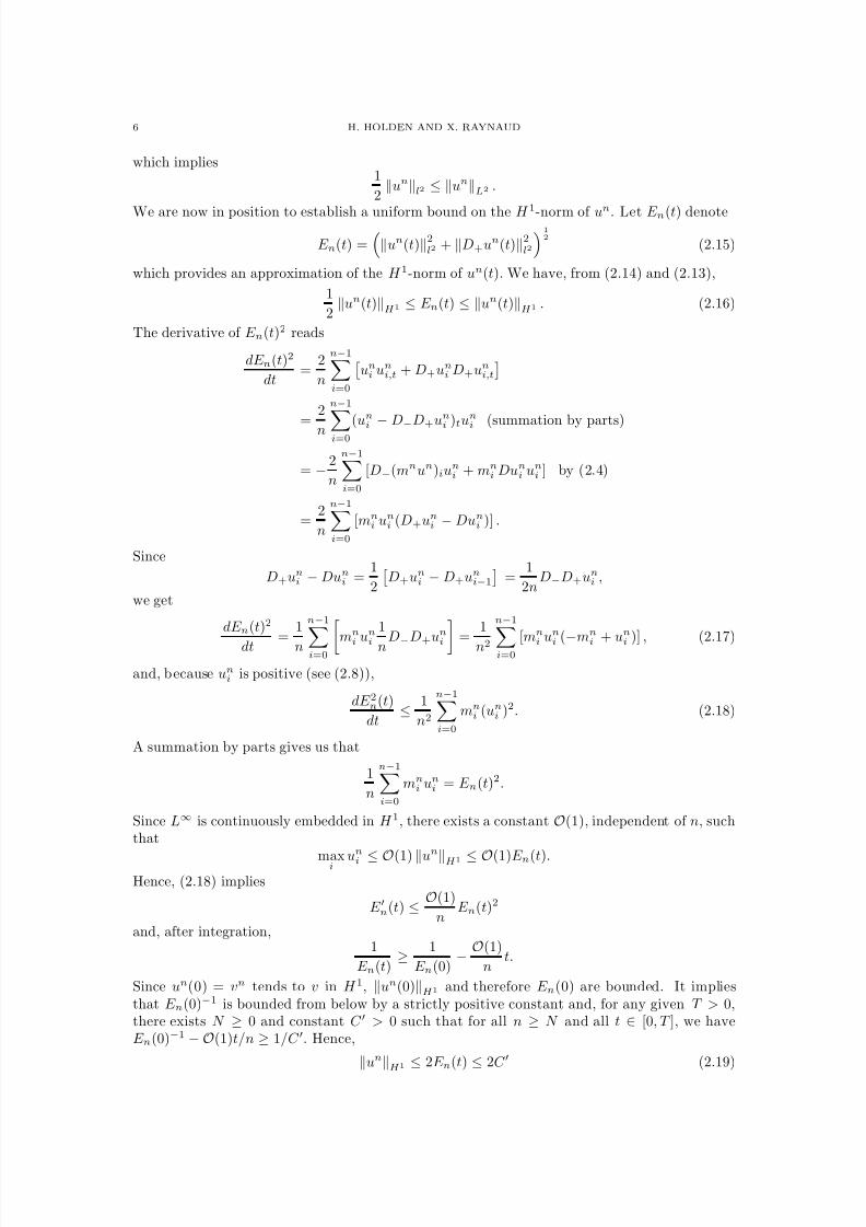
FINITE DIFFERENCE SCHEME FOR THE CAMASSA–HOLM EQUATION 7
and, by (2.16), the H 1-norm of un(t) is uniformly bounded in [0, T ]. This result also guaranteesthe existence of solutions to (2.4) in [0, T ] (at least, for n big enough) because, on [0, T ], we havethat maxi
|uni (t)
|=
un(
·, t)
L∞
≤ O(1)
un(t)
H 1 remains bounded.
To prove that we can extract a converging subsequence of un, we need some estimates on thederivative of un.
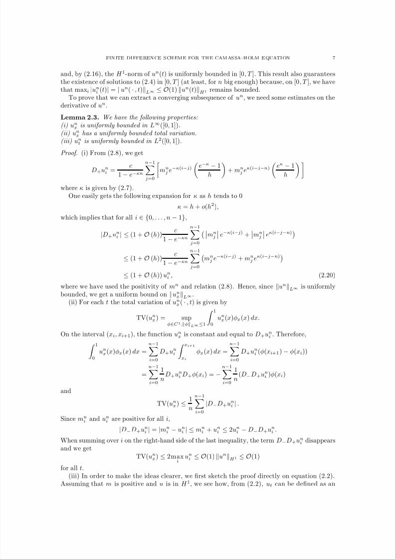
Lemma 2.3. We have the following properties:(i) unx is uniformly bounded in L∞([0, 1]).(ii) unx has a uniformly bounded total variation.(iii) unt is uniformly bounded in L2([0, 1]).
Proof. (i) From (2.8), we get
D+uni =c
1 − e−κn
n−1j=0
mnj e−κ(i−j)
e−κ − 1
h
+ mn
j eκ(i−j−n)
eκ − 1
h
where κ is given by (2.7).
One easily gets the following expansion for κ as h tends to 0κ = h + o(h2),
which implies that for all i ∈ {0, . . . , n − 1},
|D+uni | ≤ (1 + O (h))c
1 − e−κn
n−1j=0
mnj
e−κ(i−j) +mn
j
eκ(i−j−n)
≤ (1 + O (h))c
1 − e−κn
n−1j=0
mnj e−κ(i−j) + mn
j eκ(i−j−n)
≤ (1 + O (h)) uni , (2.20)
where we have used the positivity of mn and relation (2.8). Hence, since
un
L∞ is uniformly
bounded, we get a uniform bound on unxL∞.(ii) For each t the total variation of unx( · , t) is given by
TV(unx) = supφ∈C 1,φL∞≤1
1
0
unx(x)φx(x) dx.
On the interval (xi, xi+1), the function unx is constant and equal to D+uni . Therefore, 1
0
unx(x)φx(x) dx =
n−1i=0
D+uni
xi+1xi
φx(x) dx =
n−1i=0
D+uni (φ(xi+1) − φ(xi))
=
n−1i=0
1
nD+uni D+φ(xi) = −
n−1i=0
1
n(D−D+uni )φ(xi)
and
TV(unx) ≤ 1
n
n−1i=0
|D−D+uni | .
Since mni and uni are positive for all i,
|D−D+uni | = |mni − uni | ≤ mn
i + uni ≤ 2uni − D−D+uni .
When summing over i on the right-hand side of the last inequality, the term D−D+uni disappearsand we get
TV(unx) ≤ 2maxi
uni ≤ O(1) unH 1 ≤ O(1)
for all t.(iii) In order to make the ideas clearer, we first sketch the proof directly on equation (2.2).
Assuming that m is positive and u is in H 1, we see how, from (2.2), ut can be defined as an
8/3/2019 Xavier Raynaud- On a Shallow Water Wave Equation
http://slidepdf.com/reader/full/xavier-raynaud-on-a-shallow-water-wave-equation 26/161
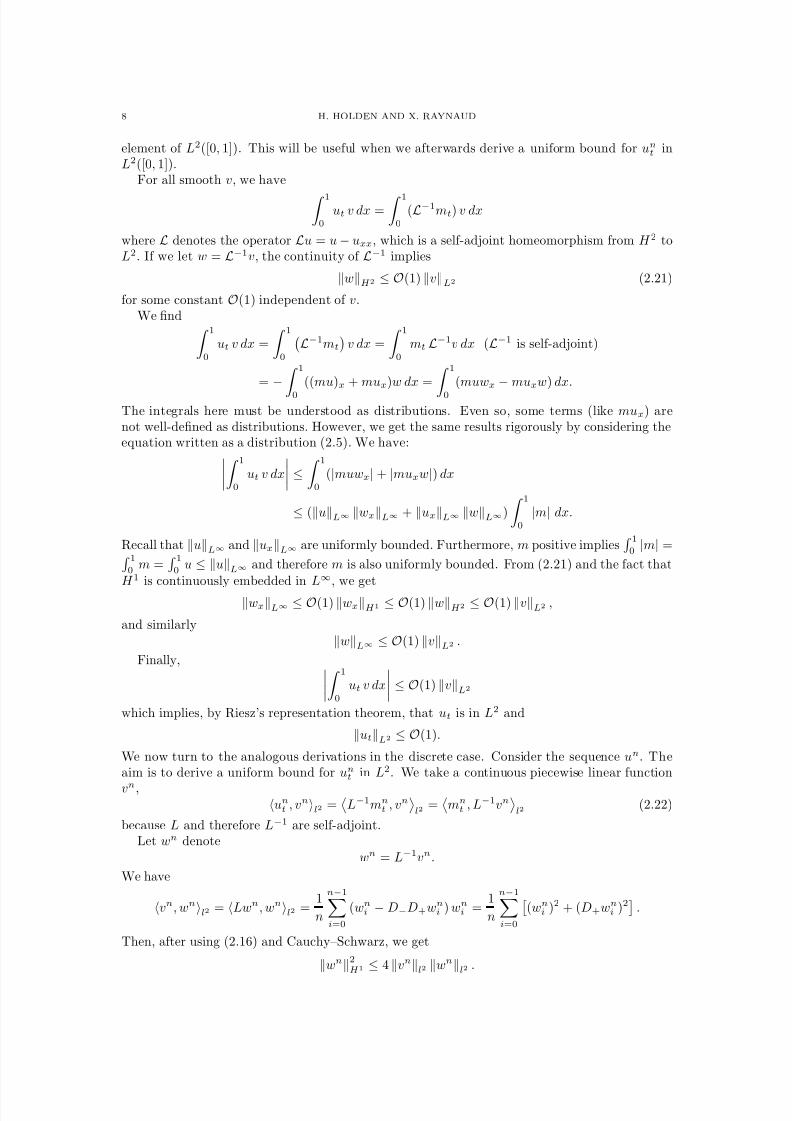
8 H. HOLDEN AND X. RAYNAUD
element of L2([0, 1]). This will be useful when we afterwards derive a uniform bound for unt inL2([0, 1]).
For all smooth v, we have 1
0
ut v dx = 1
0
(L−1mt) v dx
where L denotes the operator Lu = u − uxx, which is a self-adjoint homeomorphism from H 2 toL2. If we let w = L−1v, the continuity of L−1 implies
wH 2 ≤ O(1) vL2 (2.21)
for some constant O(1) independent of v.We find 1
0
ut v dx =
1
0
L−1mt
v dx =
1
0
mt L−1v dx (L−1 is self-adjoint)
=
− 1
0
((mu)x + mux)w dx = 1
0
(muwx
−muxw) dx.
The integrals here must be understood as distributions. Even so, some terms (like mux) arenot well-defined as distributions. However, we get the same results rigorously by considering theequation written as a distribution (2.5). We have:
1
0
ut v dx
≤ 1
0
(|muwx| + |muxw|) dx
≤ (uL∞ wxL∞ + uxL∞ wL∞)
1
0
|m| dx.
Recall that uL∞ and uxL∞ are uniformly bounded. Furthermore, m positive implies 1
0|m| =
1
0m =
1
0u ≤ uL∞ and therefore m is also uniformly bounded. From (2.21) and the fact that
H 1 is continuously embedded in L∞, we get
wxL∞ ≤ O(1) wxH 1 ≤ O(1) wH 2 ≤ O(1) vL2 ,
and similarlywL∞ ≤ O(1) vL2 .
Finally, 1
0
ut v dx
≤ O(1) vL2which implies, by Riesz’s representation theorem, that ut is in L2 and
utL2 ≤ O(1).
We now turn to the analogous derivations in the discrete case. Consider the sequence un. Theaim is to derive a uniform bound for unt in L2. We take a continuous piecewise linear function
vn,unt , vnl2 =
L−1mn
t , vnl2
=
mnt , L−1vn
l2
(2.22)
because L and therefore L−1 are self-adjoint.Let wn denote
wn = L−1vn.
We have
vn, wnl2 = Lwn, wnl2 =1
n
n−1i=0
(wni − D−D+wn
i ) wni =
1
n
n−1i=0
(wn
i )2 + (D+wni )2
.
Then, after using (2.16) and Cauchy–Schwarz, we get
wn2H 1 ≤ 4 vnl2 wnl2 .
8/3/2019 Xavier Raynaud- On a Shallow Water Wave Equation
http://slidepdf.com/reader/full/xavier-raynaud-on-a-shallow-water-wave-equation 27/161
FINITE DIFFERENCE SCHEME FOR THE CAMASSA–HOLM EQUATION 9
By (2.14), (2.16) we find
wn2H 1 ≤ O(1) vnl2 wnH 1
and
wnH 1 ≤ O(1) vnl2 (2.23)
where O(1) is a constant independent of n. Since H 1 is continuously embedded in L∞, we get
maxi
|wni | ≤ O(1) vnl2 . (2.24)
Let us define yn as follows
yni = (D+wn)i−1.
We want to find a bound on yn. From (2.14) and (2.23), we get
ynl2 ≤ wnH 1 ≤ O(1) vnl2 . (2.25)
We also have, using the definition of yn and wn,
D+yn = D−D+wn = wn − vn
which givesD+ynl2 ≤ O(1) vnl2 (2.26)
because, by (2.23),
wnl2 ≤ O(1) vnl2 .
Equations (2.25), (2.26), and (2.16) give us a uniform bound on the H 1 norm of yn:
ynH 1 ≤ O(1) vnl2 .
Since H 1 is continuously embedded in L∞, we get
maxi
|D+wni | = max
i|yni | = ynL∞ ≤ O(1) vnl2 . (2.27)
Going back to (2.22), we have
un
t , vn
l2 = mn
t , wn
l2 = −D−(mn
un
) − mn
Dun
, wn
l2= mnun, D+wnl2 − mnDun, wnl2 .
Hence,
|unt , vnl2 | ≤1
n
maxi
|uni | maxi
|D+wni | + max
i|D+uni | max
i|wn
i | n−1i=0
|mni | .
The functions uni and D+uni are uniformly bounded with respect to n. and
1
n
n−1i=0
|mni | =
1
n
n−1i=0
mni (mn is positive)
=1
n
n−1
i=0
uni
(cancellation of n−1
i=0
D−D+uni
)
≤ O(1). (uni is bounded)
Finally, using the bounds we have derived on wn, see (2.24), and D+wn, see (2.27), we get
|unt , vnl2 | ≤ O(1) vnl2 .
Taking vn = unt yields
unt l2 ≤ O(1)
which, since the l2 and L2 norm are uniformly equivalent, gives us a uniform bound on unt L2.
To prove the existence of a converging subsequence of un in C ([0, T ], H 1) we recall the followingcompactness theorem given by Simon [21, Corollary 4].
8/3/2019 Xavier Raynaud- On a Shallow Water Wave Equation
http://slidepdf.com/reader/full/xavier-raynaud-on-a-shallow-water-wave-equation 28/161
10 H. HOLDEN AND X. RAYNAUD
Theorem 2.4 (Simon). Let X,B,Y be three continuously embedded Banach spaces
X ⊂ B ⊂ Y
with the first inclusion, X ⊂ B, compact. We consider a set F of functions mapping [0, T ] intoX . If F is bounded in L∞([0, T ], X ) and ∂ F
∂t=∂f ∂t
| f ∈ F
is bounded in Lr([0, T ], Y ) where
r > 1, then F is relatively compact in C ([0, T ], B).
We now turn to the proof of our main theorem.
Proof of Theorem 2.1. (i) First we establish that there exists a subsequence of un that convergesin C ([0, T ], H 1) to an element u ∈ H 1. To apply Theorem 2.4, we have to determine the Banachspaces with the required properties. In our case, we take X as the set of functions of H 1 whichhave derivatives of bounded variation:
X =
v ∈ H 1 | vx ∈ BV
.
X endowed with the norm
vX = vH 1 + vxBV = vH 1 + vxL∞ + TV(vx)
is a Banach space. Let us prove that the injection X ⊂ H 1 is compact. We consider a sequencevn which is bounded in X . Since vnL∞ is bounded (H 1 ⊂ L∞ continuously), there exists apoint x0 such that vn(x0) is bounded and we can extract a subsequence (that we still denote vn)such that vn(x0) converges to some l ∈ R. By Helly’s theorem, we can also extract a subsequencesuch that
vn,x → w a.e. (2.28)
for some w ∈ L∞. By Lebesgue’s dominated convergence theorem, it implies that vn,x → w inL2. We set
v(x) = l +
x
x0
w(s) ds.
We have that vx = w almost everywhere. We also have
vn(x) = vn(x0) +
xx0
vn,x(s) ds
which together with (2.28) implies that vn converges to v in L∞. Therefore vn converges to v inH 1 and X is compactly embedded in H 1.
The estimates we have derived previously give us that un and unt are uniformly boundedin L∞([0, T ], X ) and L∞([0, T ], L2), respectively. Since X ⊂ H 1 ⊂ L2 with the first inclu-sion compact, Simon’s theorem gives us the existence of a subsequence of un that converges inC ([0, T ], H 1) to some u ∈ H 1.
(ii) Next we show that the limit we get is a solution of the Camassa–Holm equation (1.2).Let us now take ϕ in C ∞([0, 1] × [0, T ]) and multiply, for each i, the first equation in (2.4) by
hϕ(xi, t). We denote ϕn
the continuous piecewise linear function given by ϕn
(xi, t) = ϕ(xi, t).We sum over i and get, after one summation by parts,
n−1i=0
h
uni,t − (D−D+uni )t
ϕni =
n−1i=0
h(uni )2D+ϕi A
−n−1i=0
huni D−D+uni D+ϕni
B
−n−1i=0
huni Duni ϕni
C
+n−1i=0
hD−D+uni Duni ϕni
D
. (2.29)
We are now going to prove that each term in this equality converges to the corresponding termsin (2.5).
8/3/2019 Xavier Raynaud- On a Shallow Water Wave Equation
http://slidepdf.com/reader/full/xavier-raynaud-on-a-shallow-water-wave-equation 29/161
FINITE DIFFERENCE SCHEME FOR THE CAMASSA–HOLM EQUATION 11
Term A: We want to prove that
(un)2D+ϕn
→ 1
0
u2ϕx dx, (2.30)
where we have introduced the following notation
u = hn−1i=0
ui
to denote the average of a quantity u. We have 1
0
u2ϕx dx − (un)2D+ϕn
≤ 1
0
(u2 − (un)2)ϕx dx
+
1
0
(un)2(ϕx − D+ϕn) dx
+ 1
0 (u
n
)
2
D+ϕ
n
dx − (u
n
)
2
D+ϕ
n .
The first term tends to zero because un → u in L2 for all t ∈ [0, T ]. The second tends to zeroby Lebesgue’s dominated convergence theorem. It remains to prove that the last term tends tozero.
The integral of a product between two continuous piecewise linear function, v and w, and apiecewise constant function z can be computed explicitly. We skip the details of the calculationand give directly the result: 1
0
zvwdx =1
3zS +vS +w +
1
6zS +vw +
1
6zvS +w +
1
3zvw . (2.31)
Here S + and S − denote shift operators
(S ±u)i = ui±1
.
After using (2.31) with v = w = un and z = D+ϕn, we get 1
0
(un)2D+ϕn − (un)2D+ϕn
=
1
3(S +un − un)D+ϕnun
+1
3
(un)2D+(S −ϕn − ϕn)
.
We use the uniform equivalence of the l2 and L2 norm to get the following estimate
(S +un − un)D+ϕnun ≤ S +un − unl2 D+ϕnunl2 (Cauchy–Schwarz)
≤ O(1) un( · + h) − un( · )L2 . (2.32)
Since un ∈ H 1, we have (see, for example, [1]):
un( · + h) − un( · )L2 ≤ h unxL2 ≤ O(1)h
because unxL∞ is uniformly bounded. Hence |(S +un − un)D+ϕnun| tends to zero. The
quantity
(un)2D+(S −ϕn − ϕn)
tends to zero because ϕ is C ∞ and un uniformly bounded. Wehave proved (2.30).
Term B: We want to prove
unD−D+unD+ϕn → 1
2
1
0
u2ϕxxx dx − 1
0
u2xϕx. (2.33)
We rewrite unD−D+un in such a way that the discrete double derivative D−D+ does not appearin a product (so that we can later sum by parts). We have
unD−D+un =1
2
(D−D+((un)2)
−D+unD+un
−D−unD−un).
8/3/2019 Xavier Raynaud- On a Shallow Water Wave Equation
http://slidepdf.com/reader/full/xavier-raynaud-on-a-shallow-water-wave-equation 30/161
12 H. HOLDEN AND X. RAYNAUD
We can prove in the same way as we did for term A that
D−D+((un)2)D+ϕn
=
(un)2D−D+D+ϕn
(summation by parts)
→ 1
0
u2ϕxxx dx.
The quantity (unx)2ϕnx is a piecewise constant function. Therefore, 1
0
(unx)2ϕnx dx = D+unD+unD+ϕn .
Since unx → in L2 for all t ∈ [0, T ], and 1
0
u2xϕx dx − D+unD+unD+ϕn =
1
0
(u2x − (unx)2)ϕx dx +
1
0
(unx)2(ϕx − ϕnx) dx,
we have
D+unD+unD+ϕn → 1
0u2xϕx dx.
In the same way, we get
D−uni D−uni D+ϕn → 1
0
u2xϕx
and (2.33) is proved.Term C: We want to prove
unDunϕn → 1
0
uuxϕdx. (2.34)
We have
1
0
uuxϕ dx − unD+unϕn = 1
0
(u − un)uxϕ dx + 1
0
un(ux − unx)ϕ dx
+
1
0
ununx(ϕ − ϕn) dx +
1
0
ununxϕn dx
− unD+unϕn .
The first two terms converge to zero because un → u in H 1 for all t ∈ [0, T ]. The third termconverges to zero by Lebesgue’s dominated convergence theorem. We use formula (2.31) toevaluate the last integral: 1
0
ununxϕn dx =1
3D+unS +unS +ϕn +
1
6D+unS +unϕn
+ 16 D+ununS +ϕn + 13 D+ununϕn .
Using the same type of arguments as those we have just used for term A, one can show that 1
0
ununxϕn dx → D+ununϕn .
Thus, in order to prove (2.34), it remains to prove that
D+ununϕn − Dununϕn → 0. (2.35)
Since D = 12
(D+ + D−), we have:
D+ununϕn
− Dununϕn
=
1
2 (D+un
−D−un)unϕn

8/3/2019 Xavier Raynaud- On a Shallow Water Wave Equation
http://slidepdf.com/reader/full/xavier-raynaud-on-a-shallow-water-wave-equation 31/161
FINITE DIFFERENCE SCHEME FOR THE CAMASSA–HOLM EQUATION 13
and
|(D+un − D−un)unϕn| ≤ C n−1
i=0
h D+uni − D+uni−1≤ O(1)
1
0
|unx(x) − unx(x − h)| dx
≤ O(1)h TV(unx).
Since TV(unx) is uniformly bounded, (2.35) holds and we have proved (2.34).Term D: We want to prove that
D−D+unDunϕn → −1
2
1
0
u2xϕx dx. (2.36)
We have
1
2 1
0
u2xϕx dx+ D−D+unDunϕn (2.37)
=1
2
1
0
(u2x − (unx)2)ϕx dx +
1
2
1
0
(unx)2(ϕx − D−ϕn) dx (2.38)
− 1
2D+(D+unD+un)ϕn + D−D+unDunϕn . (2.39)
The two first terms on the right-hand side tend to zero. After using the following identity
D+(D+unD+un) = D+D+unD+un + D+D+unD+S +un,
we can rewrite the two last terms in (2.37) as
− 1
2D+(D+unD+un)ϕn + D−D+unDunϕn
=
−
1
2 D−D+S +unD+unϕn
−
1
2 D−D+S +unD+S +unϕn
+
1
2D−D+unD+S −unϕn +
1
2D−D+unD+unϕn
=1
2D−D+unD−un(ϕn − S −ϕn) +
1
2D−D+unD+un(ϕn − S −ϕn)
which tends to zero because, as we have seen before, due to the positivity of m, |D−D+uni D+uni |is uniformly bounded. We have proved (2.36).
Up to now we have not really considered the time variable. We integrate (2.29) with respectto time and integrate by part the left-hand side: T
0
n−1i=0
h
uni,t − D−D+uni,t
ϕ(xi, t) dt = − T
0
n−1i=0
h (uni − D−D+uni ) ϕt(xi, t) dt
+ n−1i=0
h (uni − D−D+uni ) ϕ(xi, t)t=T
t=0
and, after summing by parts, the limit of this expression is (we use Lebesgue’s dominated con-vergence theorem with respect to x and t)
− T
0
1
0
u(ϕt − ϕtxx) dxdt +
1
0
u(ϕ − ϕxx) dx
t=T
t=0
.
It is not hard to see that the right-hand side of (2.29) is uniformly bounded by a constant andwe can integrate over time and use the Lebesgue dominated convergence theorem to concludethat u is indeed a solution of (2.5) in the sense of distribution.
The analysis in [11] shows that the weak solution of the Camassa–Holm with initial conditionssatisfying m(x, 0)
≥0 is unique. This implies that in our algorithm not only a subsequence but
8/3/2019 Xavier Raynaud- On a Shallow Water Wave Equation
http://slidepdf.com/reader/full/xavier-raynaud-on-a-shallow-water-wave-equation 32/161
14 H. HOLDEN AND X. RAYNAUD
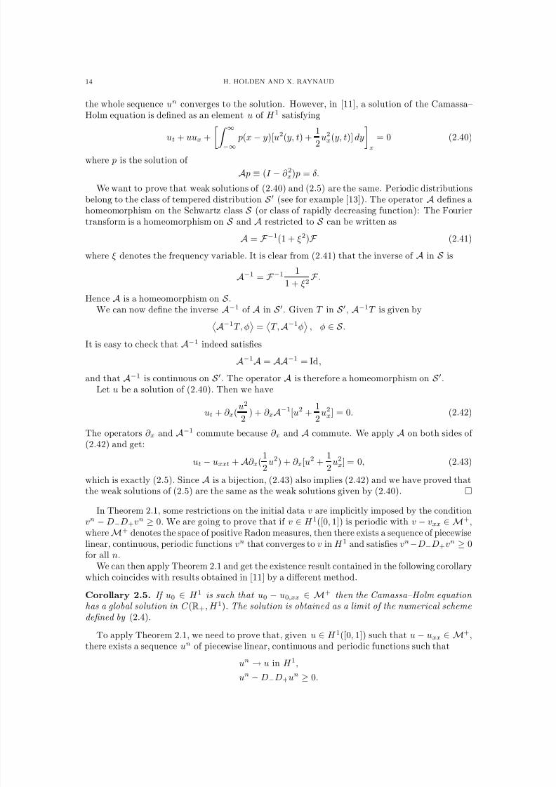
the whole sequence un converges to the solution. However, in [11], a solution of the Camassa–Holm equation is defined as an element u of H 1 satisfying
ut + uux + ∞−∞
p(x − y)[u2(y, t) +1
2 u2x(y, t)] dyx
= 0 (2.40)
where p is the solution of
A p ≡ (I − ∂ 2x) p = δ.
We want to prove that weak solutions of (2.40) and (2.5) are the same. Periodic distributionsbelong to the class of tempered distribution S (see for example [13]). The operator A defines ahomeomorphism on the Schwartz class S (or class of rapidly decreasing function): The Fouriertransform is a homeomorphism on S and A restricted to S can be written as
A = F −1(1 + ξ2)F (2.41)
where ξ denotes the frequency variable. It is clear from (2.41) that the inverse of A in S is
A−1 = F −1 11 + ξ2 F .Hence A is a homeomorphism on S .
We can now define the inverse A−1 of A in S . Given T in S , A−1T is given byA−1T, φ
=
T, A−1φ
, φ ∈ S .It is easy to check that A−1 indeed satisfies
A−1A = AA−1 = Id,
and that A−1 is continuous on S . The operator A is therefore a homeomorphism on S .Let u be a solution of (2.40). Then we have
ut + ∂ x(
u2
2 ) + ∂ xA−1
[u2
+
1
2 u2x] = 0. (2.42)
The operators ∂ x and A−1 commute because ∂ x and A commute. We apply A on both sides of (2.42) and get:
ut − uxxt + A∂ x(1
2u2) + ∂ x[u2 +
1
2u2x] = 0, (2.43)
which is exactly (2.5). Since A is a bijection, (2.43) also implies (2.42) and we have proved thatthe weak solutions of (2.5) are the same as the weak solutions given by (2.40).
In Theorem 2.1, some restrictions on the initial data v are implicitly imposed by the conditionvn − D−D+vn ≥ 0. We are going to prove that if v ∈ H 1([0, 1]) is periodic with v − vxx ∈ M+,where M+ denotes the space of positive Radon measures, then there exists a sequence of piecewiselinear, continuous, periodic functions vn that converges to v in H 1 and satisfies vn
−D−D+vn
≥0
for all n.We can then apply Theorem 2.1 and get the existence result contained in the following corollary
which coincides with results obtained in [11] by a different method.
Corollary 2.5. If u0 ∈ H 1 is such that u0 − u0,xx ∈ M+ then the Camassa–Holm equation has a global solution in C (R+, H 1). The solution is obtained as a limit of the numerical schemedefined by (2.4).
To apply Theorem 2.1, we need to prove that, given u ∈ H 1([0, 1]) such that u − uxx ∈ M+,there exists a sequence un of piecewise linear, continuous and periodic functions such that
un → u in H 1,
un − D−D+un ≥ 0.
8/3/2019 Xavier Raynaud- On a Shallow Water Wave Equation
http://slidepdf.com/reader/full/xavier-raynaud-on-a-shallow-water-wave-equation 33/161
FINITE DIFFERENCE SCHEME FOR THE CAMASSA–HOLM EQUATION 15
Let {ψni } be a partition of unity associated with the covering ∪n−1
i=0 (xi−1, xi+1). For all i ∈{0, , . . . n−1}, the functions ψn
i are non-negative with supp ψni ⊂ (xi−1, xi+1), and
n−1i=0 ψn
i = 1.Define
vni = 1h
u − uxx, ψni
and
uni − D−D+uni = vni . (2.44)
Recall that the operator un − D−D+un is invertible, see (2.8), so that un is well-defined by(2.44). Since u − uxx belongs to M+ and ψn
i ≥ 0, we have vni = uni − D−D+uni ≥ 0 and it onlyremains to prove that un converges to u in H 1. Since the application L : H 1 → H −1 given byLu = u − uxx is an homeomorphism, it is equivalent to prove that
un − unxx → u − uxx in H −1.
The homeomorphism L is also an isometry, so that
LuH −1 =
uH
1 .
We can find a bound on unH 1 . Let E n be defined, as before, by
E n =
hn−1i=0
(uni )2 + (D+un)2
i
12
.
The inequality (2.16) still holds. We have
E 2n = hn−1i=0
(uni − D−D+uni )uni
= hn−1
i=0
vni uni
≤ unL∞n−1i=0
hvni
≤ unL∞ u − uxx,n−1i=0
ψni
≤ unL∞ u − uxxM+ (sincen−1i=0
ψni = 1).
Hence, since L∞ is continuously embedded in H 1, there exists a constant C (independent of n)such that
E 2n≤
C
un
H 1
u
−uxx
M+ .
We use inequality (2.16) to get the bound on unH 1 we were looking for:
unH 1 ≤ 4C u − uxxM+ .
To prove that un− unxx → u−uxx in H −1, since un − unxxH −1 = unH 1 is uniformly bounded,we just need to prove that
un − unxx, ϕ → u − uxx, ϕfor all ϕ belonging to a dense subset of H 1 (for example C ∞).
The function un is continuous and piecewise linear. Its second derivative unxx is therefore asum of Dirac functions:
unxx =
n−1
i=0
hD−D+uni δxi
8/3/2019 Xavier Raynaud- On a Shallow Water Wave Equation
http://slidepdf.com/reader/full/xavier-raynaud-on-a-shallow-water-wave-equation 34/161
16 H. HOLDEN AND X. RAYNAUD
and, for any ϕ in C ∞, we have
un
−unxx, ϕ
=
1
0
un(x)ϕ(x) dx
−hn−1
i=0
D−D+uni ϕ(xi)
=
1
0
un(x)(ϕ(x) − ϕn(x)) dx +
1
0
un(x)ϕn(x) dx (2.45)
− hn−1i=0
uni ϕni + h
n−1i=0
viϕni
where ϕn denotes the piecewise linear, continuous function that coincides with ϕ on xi, i =0, . . . , n − 1.
The first integral in (2.45) tends to zero by the Lebesgue dominated convergence theorem.We use formula (2.31) to compute the second integral:
1
0
un(x)ϕn(x) dx =2
3 unϕn
+
1
6 S +unϕn
+
1
6 unS +ϕn
.
One can prove that this term tends to unϕn (see the proof of the convergence of term A in theproof of Theorem 2.1). The last sum equals
n−1i=0
hvni ϕ(xi) =
u − uxx,
n−1i=0
ϕni ψn
i (x)
.
For all x ∈ [0, 1], there exists a k such that x ∈ [xk , xk+1]. Then,ϕ(x) −n−1i=0
ϕni ψn
i (x)
=
n−1i=0
(ϕ(x) − ϕ(xi))ψni (x)
≤ |ϕ(x) − ϕ(xk)| + |ϕ(x) − ϕ(xk+1)|
≤2 sup
|z−y|≤h |ϕ(y)
−ϕ(z)
|and therefore, by the uniform continuity of ϕ,
n−1i=0
ϕ(xi)ψni (x) → ϕ(x) in L∞.
Thus,n−1i=0
hvni ϕ(xi) =
u − uxx,
n−1i=0
ϕ(xi)ψni
→ u − uxx, ϕ
and, from (2.45), we getun − unxx, ϕ → u − uxx, ϕ .
As already explained, it implies that
un → u in H 1.
3. Numerical results
The numerical scheme (2.4) is semi-discrete: The time derivative has not been discretized,and hence we work with a system of ordinary differential equations. However, for numericalcomputations we integrate in time by using an explicit Euler method. Given a positive time T
and l ∈ N, we consider the time step ∆t = T /l. We compute mn,lj , the approximate value of mn
at time tj = j∆t, by taking
mn,lj+1 = mn,l
j + ∆t−D−(mn,l
j un,lj ) − mn,lj Dun,lj
, (3.1)
wheremn,lj = un,lj
−D−D+un,lj . (3.2)
8/3/2019 Xavier Raynaud- On a Shallow Water Wave Equation
http://slidepdf.com/reader/full/xavier-raynaud-on-a-shallow-water-wave-equation 35/161
FINITE DIFFERENCE SCHEME FOR THE CAMASSA–HOLM EQUATION 17
0 5 10 15 20 25 30 35
0
0.5
1
1.5
2 initial condition
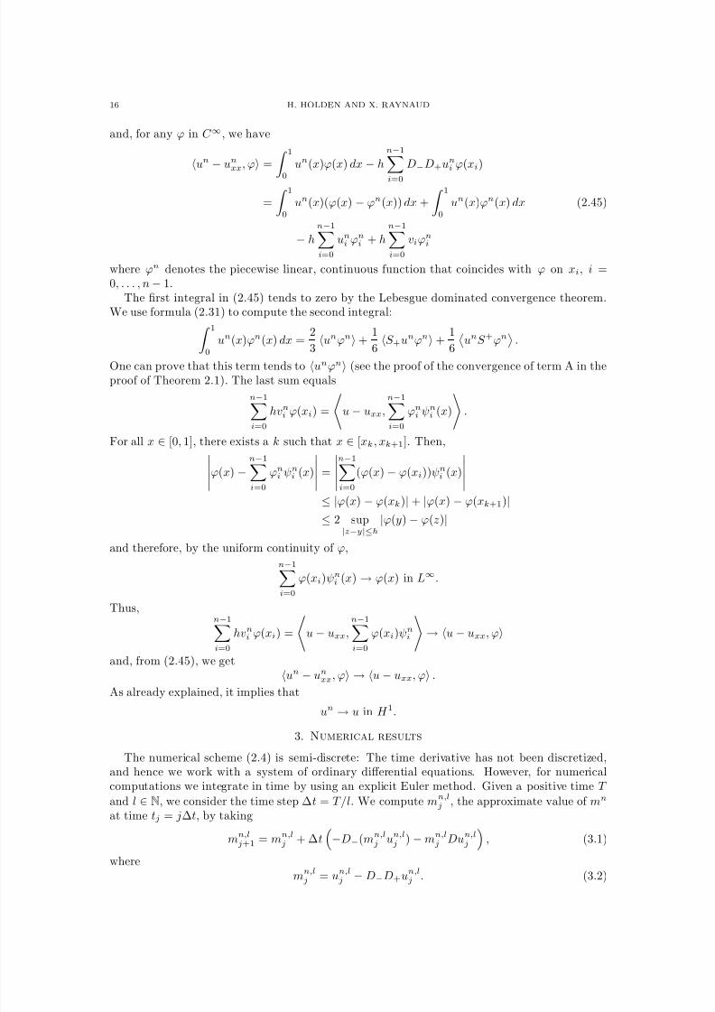
Figure 1. Periodic single peakon. The initial condition is given by u(x, 0) =
2e−|x|
and period a = 40. The computed solutions are shown at time t = 6 for(from left to right) n = 210, n = 212, n = 214 together with the exact solution(at the far right).
0 1 2 3 4 5 60
0.2
0.4
0.6
0.8
1
1.2
1.4
n=210
n=212
n=214
Figure 2. Plot of u(t) − un(t)H 1 / u(t)H 1 in the one peakon case of Figure 1.
Here mn,lj = (mn,l
0,j , . . . , mn,ln−1,j) and un,lj = (un,l0,j, . . . , un,ln−1,j). Given mn,l
j , one can still recompute
un,lj using (2.8), that is,
un,li,j = L−1mn,li,j = c
1 − e−κnn−1k=0
(e−κ(i−k) + eκ(i−k−n))mn,lk,j . (3.3)
Lemma 2.2 does not apply in this setting, and the proof of convergence for the fully discretescheme proceeds differently. Writing (2.4) as
mnt = f (mn),
where f : Rn → Rn, we observe (cf. (2.4) and (2.8)) that each component of f (x) is a polynomial
in the components x0, . . . , xn−1 of x. Hence, f is continuously differentiable. From (2.19) and(2.4), we obtain that, when n is large enough, there exists a constant C which is independent of n such that
|mni (t)
| ≤5n2 max
i
|uni (t)
| ≤Cn2
8/3/2019 Xavier Raynaud- On a Shallow Water Wave Equation
http://slidepdf.com/reader/full/xavier-raynaud-on-a-shallow-water-wave-equation 36/161
18 H. HOLDEN AND X. RAYNAUD
for all t ∈ [0, T ]. Hence, mn(t) is bounded in [0, T ] and therefore the Euler method converges,see, for example, [19], that is,
liml→∞ maxj=1,...,lm
n,l
j − mn
(tj) = 0. (3.4)
All norms are equivalent in finite dimensional vector spaces, and therefore (3.4) holds for anynorm in R
n. We denote by mn,l(t) the piecewise linear function in C ([0, T ],Rn) satisfying
mn,l(tj) = mn,lj . It is given by
mn,l(t) =1
∆t(tj+1 − t)mn,l
j +1
∆t(t − tj)mn,l
j+1
for t ∈ [tj , tj+1]. Let us prove that
liml→∞
mn,l − mnC ([0,T ],Rn)
= 0. (3.5)
We have, for t ∈ [tj , tj+1],
mn,l(t) − mn(t) =1
∆t(tj+1 − t)(mn,l
j − mn(tj)) +1
∆t(t − tj)(mn,l
j+1 − mn(tj+1))
+1
∆t(tj+1 − t)(mn(tj) − mn(t)) +
1
∆t(t − tj)(mn(tj+1) − mn(t)). (3.6)
Let ε > 0. Since mn ∈ C ([0, T ],Rn), mn is uniformly continuous and there exists δ > 0 suchthat mn(t1) − mn(t2) < ε/2 for all t1, t2 ∈ [0, T ] with |t2 − t1| < δ. We can choose l largeenough so that ∆t = T/l < δ. Then, for t ∈ [tj , tj+1], we have t − tj < δ and tj+1 − t < δ , and
1
∆t(tj+1 − t)(mn(tj) − mn(t)) +
1
∆t(t − tj)(mn(tj+1) − mn(tj+1))
<
1
∆t (tj+1 − t)ε
2 +1
∆t (t − tj)ε
2 (3.7)
<ε
2.
By (3.4), we can choose l large enough so that maxj=1,...,l
mn,lj − mn(tj)
< ε/2. Hence, 1
∆t(tj+1 − t)(mn,l
j − mn(tj)) +1
∆t(t − tj)(mn,l
j+1 − mn(tj+1))
<ε
2. (3.8)
Comparing (3.6), (3.7) and (3.8), we obtain
mn,l(t) − mn(t)
< ε
for l large enough and any t ∈ [0, T ]. Hence, (3.5) is proved. The mapping L−1
:Rn
→ Rn
,L−1mn = un, is continuous, and therefore we have
liml→∞
un,l − unC ([0,T ],Rn)
= 0.
Finally, after using the identification of Rn with the set of continuous, periodic, piecewise linearfunctions, we get that
liml→∞
un,l = un,
and, from Theorem 2.1,
limn→∞
liml→∞
un,l = u
in C ([0, T ], H 1). We summarize the result in the following theorem.
8/3/2019 Xavier Raynaud- On a Shallow Water Wave Equation
http://slidepdf.com/reader/full/xavier-raynaud-on-a-shallow-water-wave-equation 37/161
FINITE DIFFERENCE SCHEME FOR THE CAMASSA–HOLM EQUATION 19
Theorem 3.1. Let ∆t = T /l, and define the function un,li,j by (3.1)– (3.3). Define the corre-
sponding interpolating function un,l in C ([0, T ], H 1) by
un,l(x, t) =n
∆t(tj+1 − t)(xi+1 − x)u
n,li,j + (x − xi)u
n,li+1,j
+ (t − tj)
(xi+1 − x)un,li,j+1 + (x − xi)un,li+1,j+1
for x ∈ [xi, xi+1] and t ∈ [tj , tj+1]. Then
limn→∞
liml→∞
un,l = u (3.9)
in C ([0, T ], H 1) where u is the solution of the Camassa–Holm equation (1.2).
To compute the discrete spatial derivative, we need at each step to compute u from m. Thefunction u is given by a discrete convolution product
ui = hn−1
j=0
g pi−jmj.
It is advantageous to apply the Fast Fourier Transform (FFT), see [13]. In the frequency space, aconvolution product becomes a multiplication which is cheap to evaluate. Going back and forthto the frequency space is not very expensive due to the efficiency of the FFT. We use a formulaof the form (see [13] for more details):
u = F −1N (F N [g] · F N [m])
where F N denotes the FFT.We have tested algorithm (3.1) with single and double peakons. In the single peakon case,
the initial condition is given by
u(x, 0) = ccosh(d − a
2)
sinh a2
, (3.10)
which is the periodized version of u(x, 0) = ce−|x|. The period is denoted by a and d =min(x, a − x) is the distance from x to the boundary of the interval [0, a]. The peakons travelat a speed equal to their height, that is
u(x, t) = ce−|x−ct|.
If u satisfies the initial condition u(x, 0) = e−|x|, then m = 2δ at t = 0 and we take
mi(0) =
2h
if i = 0,0 otherwise,
(3.11)
as initial discrete condition. The function mi gives a discrete approximation of 2δ. Figure 1 showsthe result of the computation for different refinements. Figure 2 indicates that the computedsolution converges to the exact solution.
The sharp increase of the error u(t) − u
n
(t)H 1 at time t = 0 can be predicted by looking at(2.17) which gives a first-order approximation of the time derivative of u(t)2H 1 :
dE n(t)2
dt= −
n−1i=0
ui(hmi)2 + O (h) .
Hence,
d u2H 1
dt≈ dE n(t)2
dt≈ −4 at t = 0.
At the beginning of the computation, we can therefore expect a sharp decrease of the H 1 norm.To get convergence in H 1, it is therefore necessary that the solution becomes smooth enough so
thatdu2
H1
dt→ 0. In any case, we cannot hope for high accuracy and convergence rate in this
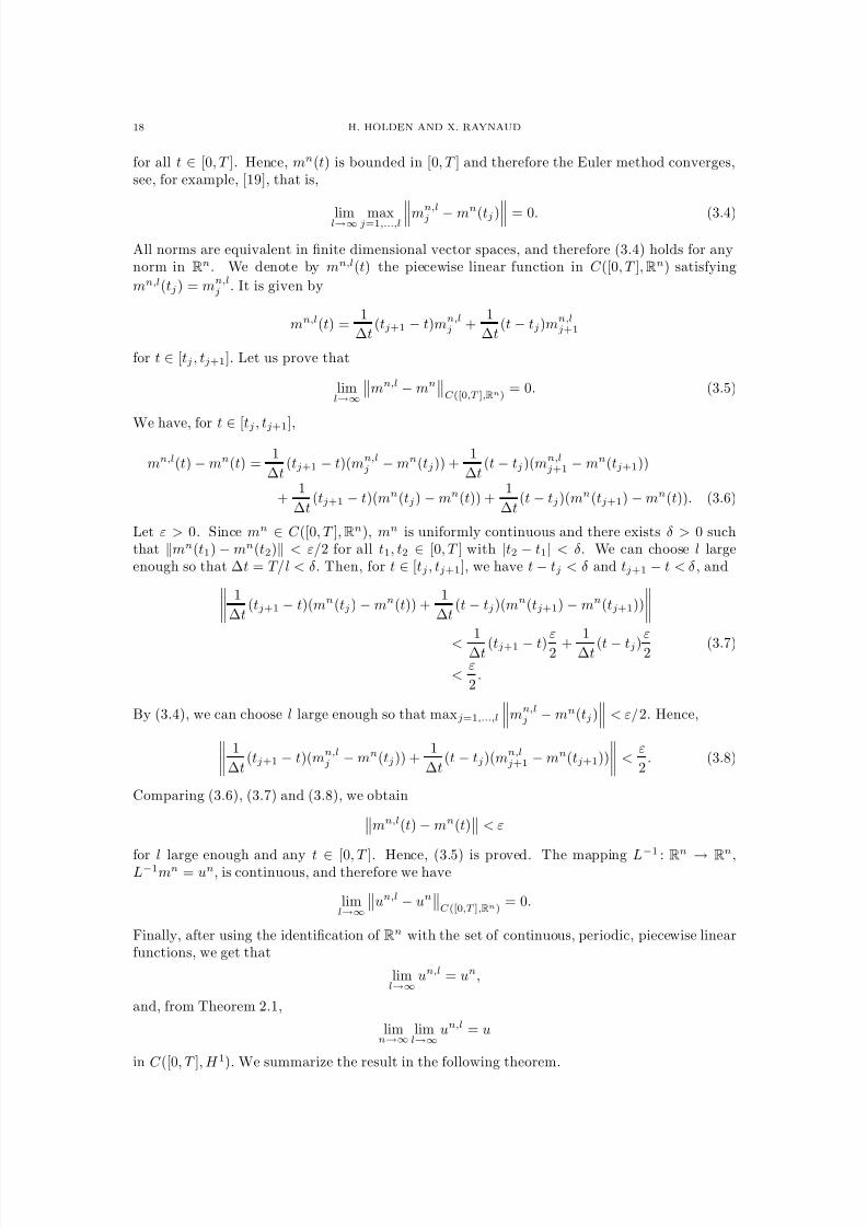
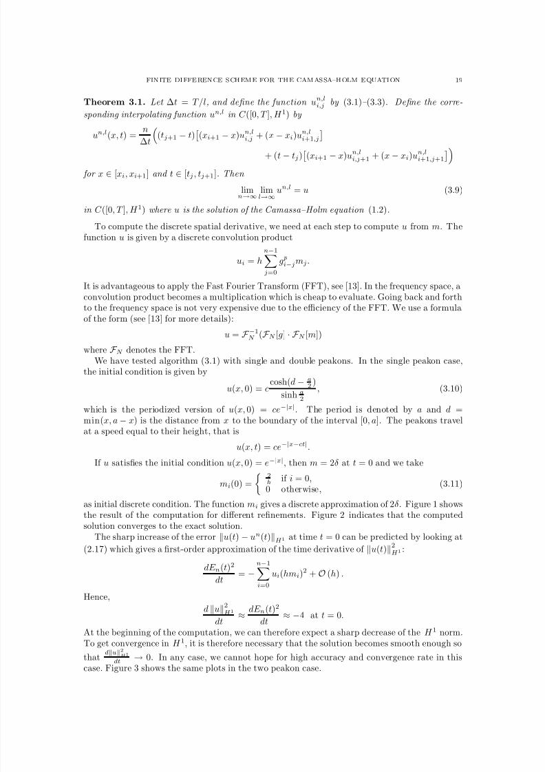
case. Figure 3 shows the same plots in the two peakon case.
8/3/2019 Xavier Raynaud- On a Shallow Water Wave Equation
http://slidepdf.com/reader/full/xavier-raynaud-on-a-shallow-water-wave-equation 38/161
20 H. HOLDEN AND X. RAYNAUD
0 5 10 15 20 25 30 35 40
0
0.2
0.4
0.6
0.8
1 ini tial condition
Figure 3. Two peakon case. The initial condition is the periodized version of
2e−|x−2|
+ e−|x−5|
. The computed solutions are shown at time t = 12 for (fromleft to right) n = 210, n = 212, n = 214 together with the exact solution (at thefar right).
0 2 4 6 8 10 120
0.2
0.4
0.6
0.8
1
1.2
1.4
n=210
n=212
n=214
Figure 4. Plot of u(t) − un(t)H 1 / u(t)H 1 in the two peakon case of Figure 3.
We have tested our algorithm with smooth initial conditions. In this case, the H 1 normremains constant in a much more accurate manner. The convergence is probably much betterbut we have no analytical solution to compare with.
Other time integration methods (second-order Runge–Kutta method, variable order Adams–Bashforth–Moulton) have also been tried and the results do not differ significantly from thosegiven by (3.1). It follows that the CH equation is not very sensitive to the way time is discretized.But the situation is completely different when we consider different space discretizations. Thefollowing schemes
mt = −D−(mu)i − miD+ui, (3.12)
mt = −D(mu)i − miDui, (3.13)
mt = −D+(mu)i − miD−ui (3.14)
are all at first glance good candidates for solving the CH equation. They preserve the H 1 norm,are finite difference approximations of (2.2) and finally look very similar to (2.4). But, testedon a single peakon, (3.12) produces a peakon that grows, (3.13) produces oscillations, and (3.14)
8/3/2019 Xavier Raynaud- On a Shallow Water Wave Equation
http://slidepdf.com/reader/full/xavier-raynaud-on-a-shallow-water-wave-equation 39/161
FINITE DIFFERENCE SCHEME FOR THE CAMASSA–HOLM EQUATION 21
behaves in a completely unexpected manner (at the first time step, m becomes a negative Diracfunction and starts traveling backward!).
Let us have a closer look at the scheme (3.12). We computedE2
n
dt:
1
2
dE 2ndt
=n−1i=0
mni,tu
ni =
n−1i=0
− D−(mnun)iui − mni D+uiui
= 0.
Thus, E n is exactly preserved. Lemma 2.2 still holds since the same proof applies to (3.12). Itallows us to derive the bounds of Lemma 2.3 and, after applying Simon’s theorem, we get theexistence of a converging subsequence. The problem is that, in general, this subsequence does not converge to the solution of the Camassa–Holm equation. In order to see that, we compare howour original algorithm (3.12) and algorithm (3.13) handle a peakon solution u = ce−|x−ct|. Theonly terms that differ are mnDun and mnD+un. We have proved earlier that, for any smoothfunction ϕ,
n−1
i=0
mni Duni ϕ(xi)
→1
2 1
0
(u2
−u2x)ϕ(x) dx
as n → ∞. In the peakon case, u2 = u2x and this term tends to zero. Roughly speaking, we can
say that mn converges to a Dirac function, see (3.11), but at the same time it is multiplied byDun which is the average of the left and right derivatives and which tends to zero at the topof the peak. Eventually the whole product mnDun tends to zero. We follow the same heuristicapproach with the term mnD+un in (3.13). This time, mn is multiplied by the right derivativeD+un of un which tends, at the top of the peak, to −c. Hence, −mnD+un tends to cδ and notzero as it would if (3.13) converged to the correct solution. This example shows how sensitivethe numerical approximation is, regarding the explicit form of the finite difference scheme, forthe Camassa–Holm equation.
Acknowledgements. HH acknowledges helpful discussions with Nils Henrik Risebro and
Kenneth H. Karlsen on discretizations of the Camassa–Holm equation.
References
[1] Haım Brezis, Analyse Fonctionnelle, Collection Mathematiques Appliquees pour la Maıtrise. [Collection of Applied Mathematics for the Master’s Degree], Masson, Paris, 1983. Theorie et applications. [Theory andapplications].
[2] Roberto Camassa, Characteristics and the initial value problem of a completely integrable shallow water
equation , Discrete Contin. Dyn. Syst. Ser. B, 3 (2003), pp. 115–139.[3] Roberto Camassa and Darryl D. Holm, An integrable shallow water equation with peaked solitons, Phys.
Rev. Lett., 71 (1993), pp. 1661–1664.[4] Roberto Camassa, Darryl D. Holm, and J. Hyman, A new integrable shallow water equation , Adv. Appl.
Mech., 31 (1994), pp. 1–33.[5] Roberto Camassa, J. Huang, and L. Lee, Integral and integrable algorithms for a nonlinear shallow-water
wave equation , Preprint. Submitted, (2004).
[6] Roberto Camassa, Jingfang Huang, and Long Lee, On a completely integrable numerical scheme for a nonlinear shallow-water wave equation , J. Nonlinear Math. Phys., 12 (2005), pp. 146–162.
[7] Adrian Constantin, On the Cauchy problem for the periodic Camassa-Holm equation , J. Differential Equa-tions, 141 (1997), pp. 218–235.
[8] , Existence of permanent and breaking waves for a shallow water equation: a geometric approach ,Ann. Inst. Fourier (Grenoble), 50 (2000), pp. 321–362.
[9] Adrian Constantin and Joachim Escher, Global existence and blow-up for a shallow water equation , Ann.Scuola Norm. Sup. Pisa Cl. Sci. (4), 26 (1998), pp. 303–328.
[10] , Well-posedness, global existence, and blowup phenomena for a periodic quasi-linear hyperbolic equa-
tion , Comm. Pure Appl. Math., 51 (1998), pp. 475–504.[11] Adrian Constantin and Luc Molinet, Global weak solutions for a shallow water equation , Comm. Math.
Phys., 211 (2000), pp. 45–61.[12] Holger R. Dullin, Georg A. Gottwald, and Darryl D. Holm, Camassa-Holm, Korteweg-de Vries-
5 and other asymptotically equivalent equations for shallow water waves, Fluid Dynam. Res., 33 (2003),pp. 73–95. In memoriam Prof. Philip Gerald Drazin 1934–2002.
8/3/2019 Xavier Raynaud- On a Shallow Water Wave Equation
http://slidepdf.com/reader/full/xavier-raynaud-on-a-shallow-water-wave-equation 40/161
22 H. HOLDEN AND X. RAYNAUD
[13] C. Gasquet and P. Witomski, Fourier Analysis and Applications, vol. 30 of Texts in Applied Mathematics,Springer-Verlag, New York, 1999. Filtering, numerical computation, wavelets, Translated from the Frenchand with a preface by R. Ryan.
[14] A. Alexandrou Himonas and Gerard Misiolek, The Cauchy problem for an integrable shallow-water
equation , Differential Integral Equations, 14 (2001), pp. 821–831.[15] Helge Holden and Xavier Raynaud, A convergent numerical scheme for the camassa–holm equation based
on multipeakons, Discrete Contin. Dyn. Syst., 14 (2006), pp. 505–523. paper II in this thesis.[16] R. S. Johnson, Camassa-Holm, Korteweg-de Vries and related models for water waves, J. Fluid Mech., 455
(2002), pp. 63–82.[17] Yi A. Li and Peter J. Olver, Well-posedness and blow-up solutions for an integrable nonlinearly dispersive
model wave equation , J. Differential Equations, 162 (2000), pp. 27–63.[18] G. Misiolek, Classical solutions of the periodic Camassa-Holm equation , Geom. Funct. Anal., 12 (2002),
pp. 1080–1104.[19] Robert Plato, Concise numerical mathematics, vol. 57 of Graduate Studies in Mathematics, American
Mathematical Society, Providence, RI, 2003. Translated from the 2000 German original by Richard Le Borneand Sabine Le Borne.
[20] Guillermo Rodrıguez-Blanco, On the Cauchy problem for the Camassa-Holm equation , Nonlinear Anal.,46 (2001), pp. 309–327.
[21] Jacques Simon, Compact sets in the space Lp(0, T ;B), Ann. Mat. Pura Appl. (4), 146 (1987), pp. 65–96.

8/3/2019 Xavier Raynaud- On a Shallow Water Wave Equation
http://slidepdf.com/reader/full/xavier-raynaud-on-a-shallow-water-wave-equation 41/161
8/3/2019 Xavier Raynaud- On a Shallow Water Wave Equation
http://slidepdf.com/reader/full/xavier-raynaud-on-a-shallow-water-wave-equation 42/161
Paper II
A convergent numerical scheme for the Camassa-Holm equation basedon multipeakons.
H. Holden and X. RaynaudPublished in Discrete Contin. Dyn. Syst. 14 (2006), no. 3, 505–523.

8/3/2019 Xavier Raynaud- On a Shallow Water Wave Equation
http://slidepdf.com/reader/full/xavier-raynaud-on-a-shallow-water-wave-equation 43/161
8/3/2019 Xavier Raynaud- On a Shallow Water Wave Equation
http://slidepdf.com/reader/full/xavier-raynaud-on-a-shallow-water-wave-equation 44/161
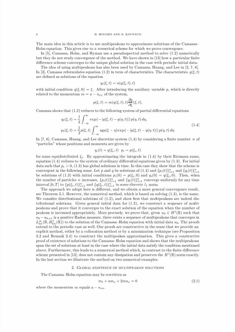
8/3/2019 Xavier Raynaud- On a Shallow Water Wave Equation
http://slidepdf.com/reader/full/xavier-raynaud-on-a-shallow-water-wave-equation 45/161
2 H. HOLDEN AND X. RAYNAUD
The main idea in this article is to use multipeakons to approximate solutions of the Camassa–Holm equation. This gives rise to a numerical scheme for which we prove convergence.
In [5], Camassa, Holm, and Hyman use a pseudospectral method to solve (1.2) numerically
but they do not study convergence of the method. We have shown in [13] how a particular finitedifference scheme converges to the unique global solution in the case with periodic initial data.
The idea of using multipeakons has also been used by Camassa, Huang, and Lee in [3, 7, 6].In [3], Camassa reformulates equation (1.2) in term of characteristics. The characteristics q(ξ, t)are defined as solutions of the equation
qt(ξ, t) = u(q(ξ, t), t)
with initial condition q(ξ, 0) = ξ. After introducing the auxiliary variable p, which is directlyrelated to the momentum m = u − uxx of the system,
p(ξ, t) = m(q(ξ, t), t)∂q
∂ξ(ξ, t),
Camassa shows that (1.2) reduces to the following system of partial differential equations
qt(ξ, t) = 12
∞
−∞
exp(− |q(ξ, t) − q(η, t)|) p(η, t) dη,
pt(ξ, t) =1
2 p(ξ, t)
∞−∞
sgn(ξ − η)exp(− |q(ξ, t) − q(η, t)|) p(η, t) dη.
(1.4)
In [7, 6], Camassa, Huang, and Lee discretize system (1.4) by considering a finite number n of “particles” whose positions and momenta are given by
qi(t) = q(ξi, t) pi = p(ξi, t)
for some equidistributed ξi. By approximating the integrals in (1.4) by their Riemann sums,equation (1.4) reduces to the system of ordinary differential equations given by (1.3). For initialdata such that pi > 0, (1.3) has global solutions in time. In this case they show that the scheme isconvergent in the following sense. Let p and q be solutions of (1.4) and
{ pi(t)
}ni=1 and
{qi(t)
}ni=1
be solutions of (1.3) with initial conditions pi(0) = p(ξi, 0) and qi(0) = q(ξi, 0). Then, whenthe number of particles n increases, { pi(t)}ni=1 and {qi(t)}ni=1 converge uniformly for any timeinterval [0, T ] to { p(ξi, t)}ni=1 and {q(ξi, t)}ni=1 in some discrete l1 norm.
The approach we adopt here is different, and we obtain a more general convergence result,see Theorem 3.1. However, the numerical method, which is based on solving (1.3), is the same.We consider distributional solutions of (1.2), and show first that multipeakons are indeed dis-tributional solutions. Given general initial data for (1.2), we construct a sequence of multi-peakons and prove that it converges to the exact solution of the equation when the number of peakons is increased appropriately. More precisely, we prove that, given u0 ∈ H 1(R) such thatu0 − u0,xx is a positive Radon measure, there exists a sequence of multipeakons that converges inL∞loc(R, H 1loc(R)) to the solution of the Camassa–Holm equation with initial data u0. The proofsextend to the periodic case as well. Our proofs are constructive in the sense that we provide an
explicit method, either by a collocation method or by a minimization technique (see Proposition3.2 and Remark 3.4) to construct the multipeakon approximation. This gives a constructiveproof of existence of solutions to the Camassa–Holm equation and shows that the multipeakonsspan the set of solutions at least in the case where the initial data satisfy the condition mentionedabove. Furthermore, this leads to a numerical method which, in contrast to the finite differencescheme presented in [13], does not contain any dissipation and preserves the H 1(R) norm exactly.In the last section we illustrate the method on two numerical examples.
2. Global existence of multipeakon solutions
The Camassa–Holm equation may be rewritten as
mt + umx + 2mux = 0 (2.1)
where the momentum m equals u
−uxx.
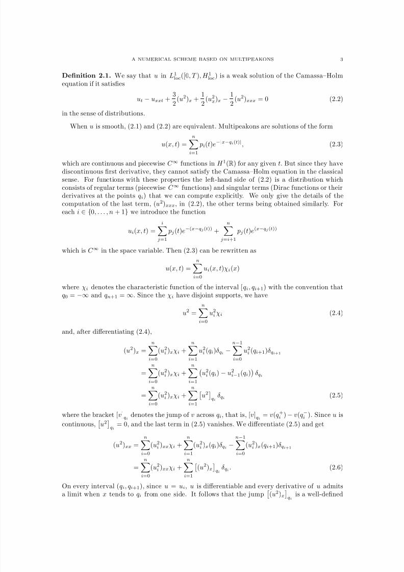
8/3/2019 Xavier Raynaud- On a Shallow Water Wave Equation
http://slidepdf.com/reader/full/xavier-raynaud-on-a-shallow-water-wave-equation 46/161
A NUMERICAL SCHEME BASED ON MULTIPEAKONS 3
Definition 2.1. We say that u in L1loc([0, T ), H 1loc) is a weak solution of the Camassa–Holm
equation if it satisfies
ut − uxxt +
3
2 (u2
)x +
1
2 (u2x)x −
1
2 (u2
)xxx = 0 (2.2)
in the sense of distributions.
When u is smooth, (2.1) and (2.2) are equivalent. Multipeakons are solutions of the form
u(x, t) =ni=1
pi(t)e−|x−qi(t)|, (2.3)
which are continuous and piecewise C ∞ functions in H 1(R) for any given t. But since they havediscontinuous first derivative, they cannot satisfy the Camassa–Holm equation in the classicalsense. For functions with these properties the left-hand side of (2.2) is a distribution whichconsists of regular terms (piecewise C ∞ functions) and singular terms (Dirac functions or theirderivatives at the points qi) that we can compute explicitly. We only give the details of thecomputation of the last term, (u2)xxx, in (2.2), the other terms being obtained similarly. Foreach i ∈ {0, . . . , n + 1} we introduce the function
ui(x, t) =
ij=1
pj(t)e−(x−qj(t)) +
nj=i+1
pj(t)e(x−qj(t))
which is C ∞ in the space variable. Then (2.3) can be rewritten as
u(x, t) =
ni=0
ui(x, t)χi(x)
where χi denotes the characteristic function of the interval [qi, qi+1) with the convention thatq0 =
−∞and qn+1 =
∞. Since the χi have disjoint supports, we have
u2 =
ni=0
u2i χi (2.4)
and, after differentiating (2.4),
(u2)x =
ni=0
(u2i )xχi +
ni=1
u2i (qi)δqi −
n−1i=0
u2i (qi+1)δqi+1
=
ni=0
(u2i )xχi +
ni=1
u2i (qi) − u2
i−1(qi)
δqi
=n
i=0
(u2i )xχi +
n
i=1u2
qi
δqi (2.5)
where the bracket [v]qi denotes the jump of v across qi, that is, [v]qi = v(q+i ) − v(q−i ). Since u is
continuous,u2qi
= 0, and the last term in (2.5) vanishes. We differentiate (2.5) and get
(u2)xx =ni=0
(u2i )xxχi +
ni=1
(u2i )x(qi)δqi −
n−1i=0
(u2i )x(qi+1)δqi+1
=ni=0
(u2i )xxχi +
ni=1
(u2)x
qi
δqi . (2.6)
On every interval (qi, qi+1), since u = ui, u is differentiable and every derivative of u admitsa limit when x tends to qi from one side. It follows that the jump (u2)xqi is a well-defined
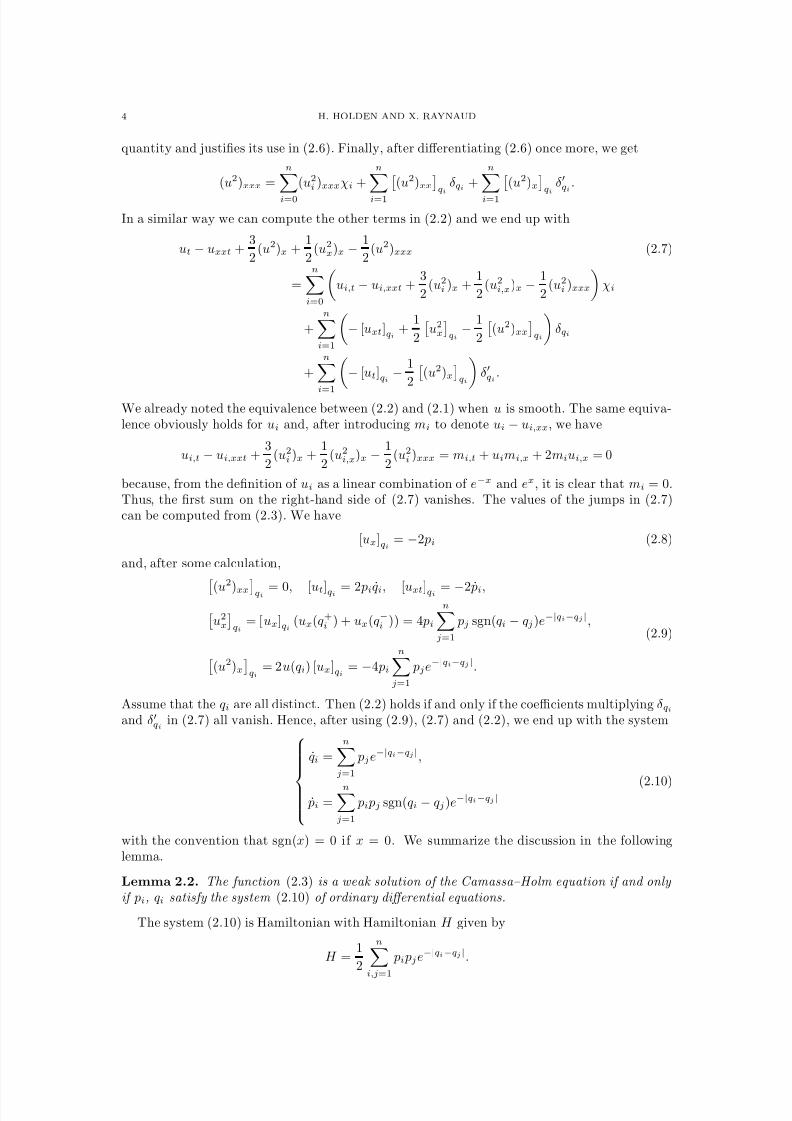
8/3/2019 Xavier Raynaud- On a Shallow Water Wave Equation
http://slidepdf.com/reader/full/xavier-raynaud-on-a-shallow-water-wave-equation 47/161
4 H. HOLDEN AND X. RAYNAUD
quantity and justifies its use in (2.6). Finally, after differentiating (2.6) once more, we get
(u2)xxx =n
i=0
(u2i )xxxχi +
n
i=1(u2)xxqi δqi +
n
i=1(u2)xqi δqi .
In a similar way we can compute the other terms in (2.2) and we end up with
ut − uxxt +3
2(u2)x +
1
2(u2
x)x − 1
2(u2)xxx (2.7)
=
ni=0
ui,t − ui,xxt +
3
2(u2
i )x +1
2(u2
i,x)x − 1
2(u2
i )xxx
χi
+
ni=1
− [uxt]qi +
1
2
u2x
qi
− 1
2
(u2)xx
qi
δqi
+
n
i=1− [ut]qi − 1
2 (u2)xqi δqi .
We already noted the equivalence between (2.2) and (2.1) when u is smooth. The same equiva-lence obviously holds for ui and, after introducing mi to denote ui − ui,xx, we have
ui,t − ui,xxt +3
2(u2
i )x +1
2(u2
i,x)x − 1
2(u2
i )xxx = mi,t + uimi,x + 2miui,x = 0
because, from the definition of ui as a linear combination of e−x and ex, it is clear that mi = 0.Thus, the first sum on the right-hand side of (2.7) vanishes. The values of the jumps in (2.7)can be computed from (2.3). We have
[ux]qi = −2 pi (2.8)
and, after some calculation,
(u
2
)xxqi = 0, [ut]qi = 2 piqi, [uxt]qi = −2 ˙ pi,
u2x
qi
= [ux]qi (ux(q+i ) + ux(q−i )) = 4 pi
nj=1
pj sgn(qi − qj)e−|qi−qj|,
(u2)x
qi
= 2u(qi) [ux]qi = −4 pi
nj=1
pje−|qi−qj |.
(2.9)
Assume that the qi are all distinct. Then (2.2) holds if and only if the coefficients multiplying δqiand δqi in (2.7) all vanish. Hence, after using (2.9), (2.7) and (2.2), we end up with the system
qi =n
j=1
pje−|qi−qj|,
˙ pi =nj=1
pi pj sgn(qi − qj)e−|qi−qj |(2.10)
with the convention that sgn(x) = 0 if x = 0. We summarize the discussion in the followinglemma.
Lemma 2.2. The function (2.3) is a weak solution of the Camassa–Holm equation if and only if pi, qi satisfy the system (2.10) of ordinary differential equations.
The system (2.10) is Hamiltonian with Hamiltonian H given by
H =1
2
n
i,j=1
pi pje−|qi−qj|.
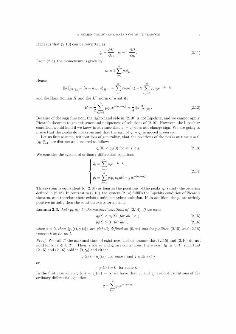
8/3/2019 Xavier Raynaud- On a Shallow Water Wave Equation
http://slidepdf.com/reader/full/xavier-raynaud-on-a-shallow-water-wave-equation 48/161
A NUMERICAL SCHEME BASED ON MULTIPEAKONS 5
It means that (2.10) can be rewritten as
qi =∂H
∂pi, ˙ pi = −∂H
∂qi. (2.11)
From (2.3), the momentum is given by
m = 2
ni=1
piδqi .
Hence,
u2H 1(R) = u − uxx, uH −1 =
ni=1
2 piu(qi) = 2n
i,j=1
pi pje−|qi−qj|.
and the Hamiltonian H and the H 1 norm of u satisfy
H =1
2
ni,j=1
pi pje−|qi−qj| =1
4u2
H 1(R) . (2.12)
Because of the sign function, the right-hand side in (2.10) is not Lipchitz, and we cannot applyPicard’s theorem to get existence and uniqueness of solutions of (2.10). However, the Lipschitzcondition would hold if we knew in advance that qi − qj does not change sign. We are going toprove that the peaks do not cross and that the sign of qi − qj is indeed preserved.
Let us first assume, without loss of generality, that the positions of the peaks at time t = 0,{qi}ni=1, are distinct and ordered as follows
qi(0) < qj(0) for all i < j. (2.13)
We consider the system of ordinary differential equations
qi =n
j=1
pje−|qi−qj |,
˙ pi =n
j=1
pi pj sgn(i − j)e−|qi−qj |.
(2.14)
This system is equivalent to (2.10) as long as the positions of the peaks qi satisfy the orderingdefined in (2.13). In contrast to (2.10), the system (2.14) fulfills the Lipchitz condition of Picard’stheorem, and therefore there exists a unique maximal solution. If, in addition, the pi are strictlypositive initially then the solution exists for all time.
Lemma 2.3. Let { pi, qi} be the maximal solutions of (2.14). If we have
qi(t) < qj(t) for all i < j, (2.15)
pi(t) > 0 for all i, (2.16)
when t = 0, then { pi(t), qi(t)} are globally defined on [0, ∞) and inequalities (2.15) and (2.16)
remain true for all t.Proof. We call T the maximal time of existence. Let us assume that (2.15) and (2.16) do nothold for all t ∈ [0, T ). Then, since pi and qi are continuous, there exist t0 in [0, T ) such that(2.15) and (2.16) hold in [0, t0) and either
qi(t0) = qj(t0) for some i and j with i < j
or pi(t0) = 0 for some i.
In the first case when qi(t0) = qj(t0) = α, we have that qi and qj are both solutions of theordinary differential equation
q =n
k=1
pke−|q−qk|
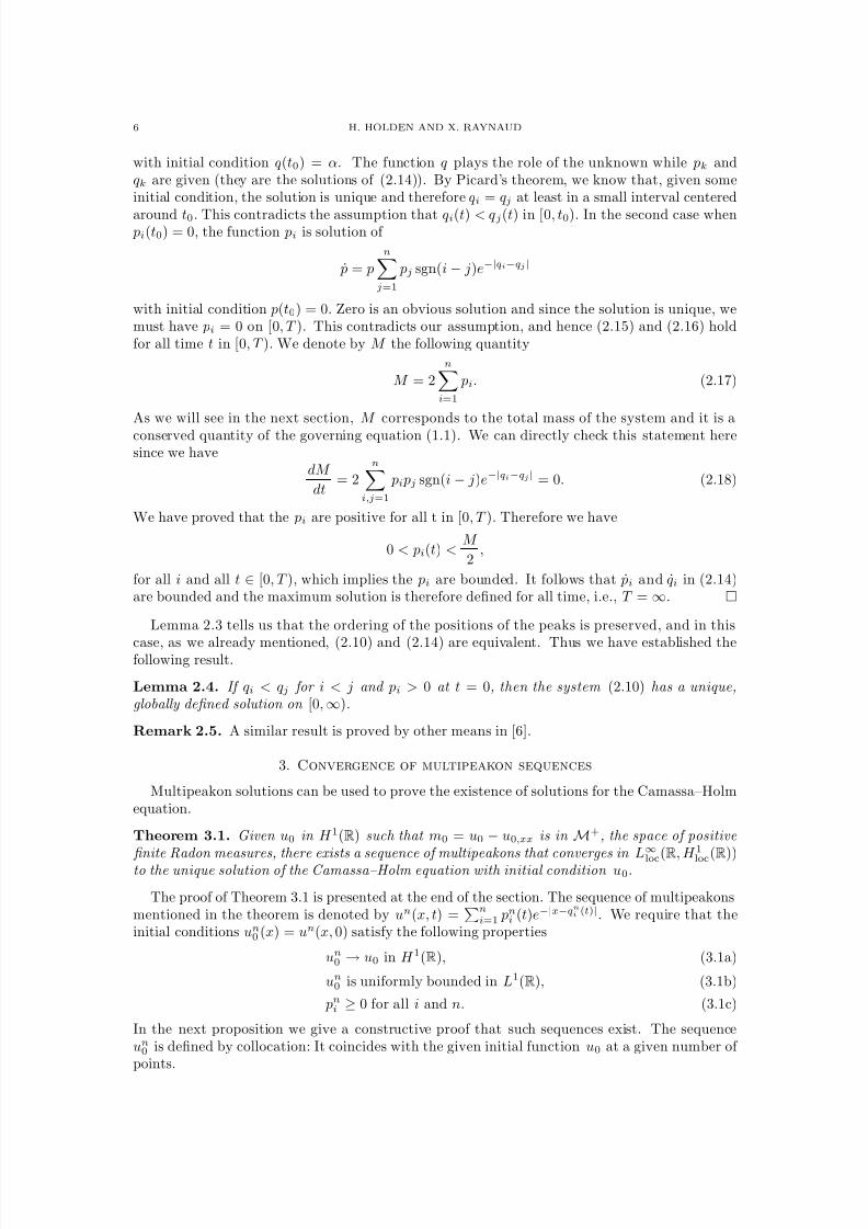
8/3/2019 Xavier Raynaud- On a Shallow Water Wave Equation
http://slidepdf.com/reader/full/xavier-raynaud-on-a-shallow-water-wave-equation 49/161
6 H. HOLDEN AND X. RAYNAUD
with initial condition q(t0) = α. The function q plays the role of the unknown while pk andqk are given (they are the solutions of (2.14)). By Picard’s theorem, we know that, given someinitial condition, the solution is unique and therefore qi = qj at least in a small interval centered
around t0. This contradicts the assumption that qi(t) < qj(t) in [0, t0). In the second case when pi(t0) = 0, the function pi is solution of
˙ p = pn
j=1
pj sgn(i − j)e−|qi−qj |
with initial condition p(t0) = 0. Zero is an obvious solution and since the solution is unique, wemust have pi = 0 on [0, T ). This contradicts our assumption, and hence (2.15) and (2.16) holdfor all time t in [0, T ). We denote by M the following quantity
M = 2
ni=1
pi. (2.17)
As we will see in the next section, M corresponds to the total mass of the system and it is a
conserved quantity of the governing equation (1.1). We can directly check this statement heresince we have
dM
dt= 2
ni,j=1
pi pj sgn(i − j)e−|qi−qj| = 0. (2.18)
We have proved that the pi are positive for all t in [0, T ). Therefore we have
0 < pi(t) <M
2,
for all i and all t ∈ [0, T ), which implies the pi are bounded. It follows that ˙ pi and qi in (2.14)are bounded and the maximum solution is therefore defined for all time, i.e., T = ∞.
Lemma 2.3 tells us that the ordering of the positions of the peaks is preserved, and in this
case, as we already mentioned, (2.10) and (2.14) are equivalent. Thus we have established thefollowing result.
Lemma 2.4. If qi < qj for i < j and pi > 0 at t = 0, then the system (2.10) has a unique,globally defined solution on [0, ∞).
Remark 2.5. A similar result is proved by other means in [6].
3. Convergence of multipeakon sequences
Multipeakon solutions can be used to prove the existence of solutions for the Camassa–Holmequation.
Theorem 3.1. Given u0 in H 1(R) such that m0 = u0 − u0,xx is in M+, the space of positive finite Radon measures, there exists a sequence of multipeakons that converges in L∞
loc(R, H 1
loc(R))
to the unique solution of the Camassa–Holm equation with initial condition u0.
The proof of Theorem 3.1 is presented at the end of the section. The sequence of multipeakonsmentioned in the theorem is denoted by un(x, t) =
ni=1 pni (t)e−|x−q
ni (t)|. We require that the
initial conditions un0 (x) = un(x, 0) satisfy the following properties
un0 → u0 in H 1(R), (3.1a)
un0 is uniformly bounded in L1(R), (3.1b)
pni ≥ 0 for all i and n. (3.1c)
In the next proposition we give a constructive proof that such sequences exist. The sequenceun0 is defined by collocation: It coincides with the given initial function u0 at a given number of points.
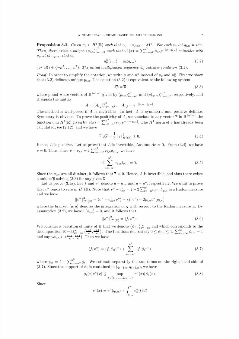
8/3/2019 Xavier Raynaud- On a Shallow Water Wave Equation
http://slidepdf.com/reader/full/xavier-raynaud-on-a-shallow-water-wave-equation 50/161
A NUMERICAL SCHEME BASED ON MULTIPEAKONS 7
Proposition 3.2. Given u0 ∈ H 1(R) such that u0 − u0,xx ∈ M+. For each n, let qi,n = i/n.
Then, there exists a unique ( pi,n)n2
i=−n2 such that un0 (x) =
n2
i=−n2 pi,ne−|x−qi,n| coincides with u0 at the qi,n, that is,
un0 (qi,n) = u0(qi,n) (3.2)
for all i ∈ {−n2, . . . , n2}. The initial multipeakon sequence un0 satisfies condition (3.1).
Proof. In order to simplify the notation, we write u and un instead of u0 and un0 . First we showthat (3.2) defines a unique pi,n. The equation (3.2) is equivalent to the following system
Ap = u (3.3)
where p and u are vectors of R2n2+1 given by ( pi,n)n2
i=−n2 and (u(qi,n))n2
i=−n2 , respectively, andA equals the matrix
A = (Ai,j)n2
i,j=−n2 , Ai,j = e−|qi,n−qj,n|.
The method is well-posed if A is invertible. In fact, A is symmetric and positive definite.
Symmetry is obvious. To prove the positivity of A, we associate to any vector r inR2n2+1
thefunction v in H 1(R) given by v(x) =n2
i=−n2 ri,ne−|x−qi,n|. The H 1 norm of v has already beencalculated, see (2.12), and we have
rtAr =1
2v2
H 1(R) ≥ 0. (3.4)
Hence, A is positive. Let us prove that A is invertible. Assume Ar = 0. From (3.4), we have
v = 0. Thus, since v − vxx = 2n2
i=−n2 ri,nδqi,n, we have
2
n2i=−n2
ri,nδqi,n = 0. (3.5)
Since the qi,n are all distinct, it follows that r = 0. Hence, A is invertible, and thus there exists
a unique p solving (3.3) for any given u.Let us prove (3.1a). Let f and vn denote u − uxx and u − un, respectively. We want to prove
that vn tends to zero in H 1(R). Note that vn − vnxx = f − 2n2
i=−n2 pi,nδqi,n is a Radon measureand we have
vn2H 1(R) = vn − vnxx, vn = f, vn − 2 pi,nvn(qi,n)
where the bracket µ, g denotes the integration of g with respect to the Radon measure µ. Byassumption (3.2), we have v(qi,n) = 0, and it follows that
vn2H 1(R) = f, vn . (3.6)
We consider a partition of unity of R that we denote {φi,n}∞i=−∞ and which corresponds to the
decomposition R = ∪∞i=−∞ i−1n
, i+1n . The functions φi,n satisfy 0 ≤ φi,n ≤ 1,
∞i=−∞ φi,n = 1
and supp φi,n ⊂ (i−1n ,
i+1n ). Then we have
f, vn = f, ψnvn +n2
i=−n2
f, φivn (3.7)
where ψn = 1 −n2
i=−n2 φi. We estimate separately the two terms on the right-hand side of (3.7). Since the support of φi is contained in (qi−1,n, qi+1,n), we have
φi(x)vn(x) ≤ supx∈(qi−1,n,qi+1,n)
|vn(x)| φi(x). (3.8)
Since
vn(x) = vn(qi,n) + x
qi,n
vnx(t) dt
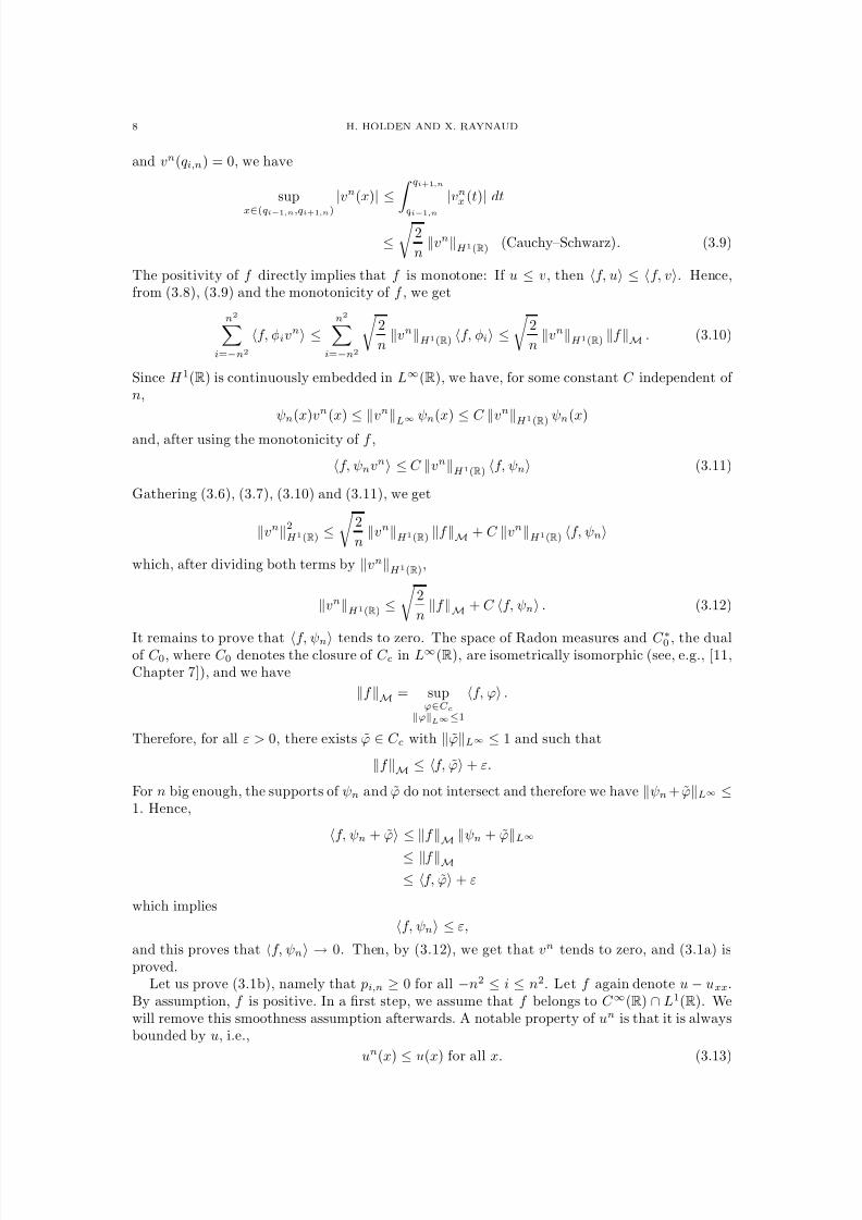
8/3/2019 Xavier Raynaud- On a Shallow Water Wave Equation
http://slidepdf.com/reader/full/xavier-raynaud-on-a-shallow-water-wave-equation 51/161
8 H. HOLDEN AND X. RAYNAUD
and vn(qi,n) = 0, we have
sup
x∈(qi−1,n,qi+1,n) |vn(x)
| ≤ qi+1,n
qi−1,n |vnx (t)
|dt
≤
2
nvnH 1(R) (Cauchy–Schwarz). (3.9)
The positivity of f directly implies that f is monotone: If u ≤ v, then f, u ≤ f, v. Hence,from (3.8), (3.9) and the monotonicity of f , we get
n2i=−n2
f, φivn ≤
n2i=−n2
2
nvnH 1(R) f, φi ≤
2
nvnH 1(R) f M . (3.10)
Since H 1(R) is continuously embedded in L∞(R), we have, for some constant C independent of n,
ψn(x)vn(x)
≤ vn
L∞ ψn(x)
≤C
vn
H 1(R) ψn(x)
and, after using the monotonicity of f ,
f, ψnvn ≤ C vnH 1(R) f, ψn (3.11)
Gathering (3.6), (3.7), (3.10) and (3.11), we get
vn2H 1(R) ≤
2
nvnH 1(R) f M + C vnH 1(R) f, ψn
which, after dividing both terms by vnH 1(R),
vnH 1(R) ≤
2
nf M + C f, ψn . (3.12)
It remains to prove that f, ψn tends to zero. The space of Radon measures and C ∗0 , the dual
of C 0, where C 0 denotes the closure of C c in L∞(R), are isometrically isomorphic (see, e.g., [11,Chapter 7]), and we have
f M = supϕ∈C c
ϕL∞≤1
f, ϕ .
Therefore, for all ε > 0, there exists ϕ ∈ C c with ϕL∞ ≤ 1 and such that
f M ≤ f, ϕ + ε.
For n big enough, the supports of ψn and ϕ do not intersect and therefore we have ψn+ ϕL∞ ≤1. Hence,
f, ψn + ϕ ≤ f M ψn + ϕL∞≤ f M≤ f, ϕ + ε
which implies
f, ψn ≤ ε,
and this proves that f, ψn → 0. Then, by (3.12), we get that vn tends to zero, and (3.1a) isproved.
Let us prove (3.1b), namely that pi,n ≥ 0 for all −n2 ≤ i ≤ n2. Let f again denote u − uxx.By assumption, f is positive. In a first step, we assume that f belongs to C ∞(R) ∩ L1(R). Wewill remove this smoothness assumption afterwards. A notable property of un is that it is alwaysbounded by u, i.e.,
un(x)
≤u(x) for all x. (3.13)
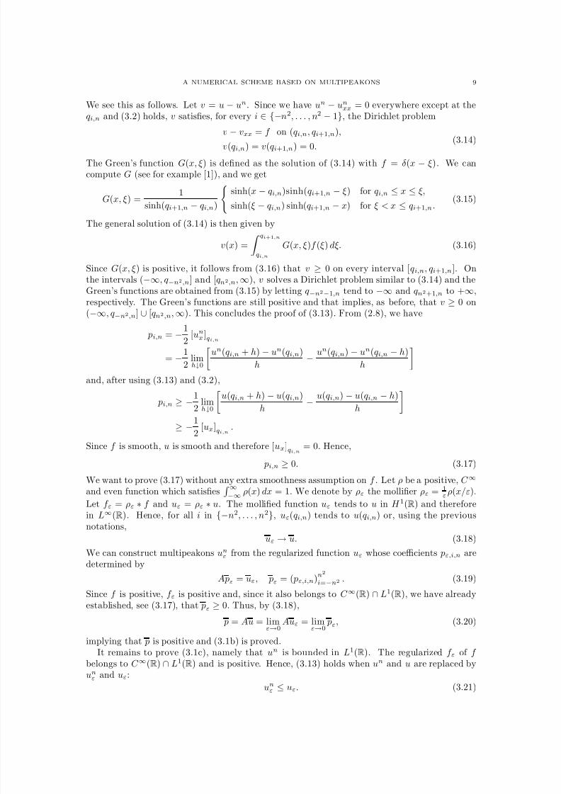
8/3/2019 Xavier Raynaud- On a Shallow Water Wave Equation
http://slidepdf.com/reader/full/xavier-raynaud-on-a-shallow-water-wave-equation 52/161
A NUMERICAL SCHEME BASED ON MULTIPEAKONS 9
We see this as follows. Let v = u − un. Since we have un − unxx = 0 everywhere except at theqi,n and (3.2) holds, v satisfies, for every i ∈ {−n2, . . . , n2 − 1}, the Dirichlet problem
v−
vxx = f on (qi,n, qi+1,n),
v(qi,n) = v(qi+1,n) = 0. (3.14)
The Green’s function G(x, ξ) is defined as the solution of (3.14) with f = δ(x − ξ). We cancompute G (see for example [1]), and we get
G(x, ξ) =1
sinh(qi+1,n − qi,n)
sinh(x − qi,n)sinh(qi+1,n − ξ) for qi,n ≤ x ≤ ξ,
sinh(ξ − qi,n) sinh(qi+1,n − x) for ξ < x ≤ qi+1,n.(3.15)
The general solution of (3.14) is then given by
v(x) =
qi+1,nqi,n
G(x, ξ)f (ξ) dξ. (3.16)
Since G(x, ξ) is positive, it follows from (3.16) that v
≥0 on every interval [qi,n, qi+1,n]. On
the intervals (−∞, q−n2,n] and [qn2,n, ∞), v solves a Dirichlet problem similar to (3.14) and theGreen’s functions are obtained from (3.15) by letting q−n2−1,n tend to −∞ and qn2+1,n to +∞,respectively. The Green’s functions are still positive and that implies, as before, that v ≥ 0 on(−∞, q−n2,n] ∪ [qn2,n, ∞). This concludes the proof of (3.13). From (2.8), we have
pi,n = −1
2[unx ]qi,n
= −1
2limh↓0
un(qi,n + h) − un(qi,n)
h− un(qi,n) − un(qi,n − h)
h
and, after using (3.13) and (3.2),
pi,n ≥ −1
2limh↓0
u(qi,n + h) − u(qi,n)
h− u(qi,n) − u(qi,n − h)
h ≥ −1
2[ux]qi,n .
Since f is smooth, u is smooth and therefore [ux]qi,n = 0. Hence,
pi,n ≥ 0. (3.17)
We want to prove (3.17) without any extra smoothness assumption on f . Let ρ be a positive, C ∞
and even function which satisfies ∞−∞
ρ(x) dx = 1. We denote by ρε the mollifier ρε = 1ερ(x/ε).
Let f ε = ρε ∗ f and uε = ρε ∗ u. The mollified function uε tends to u in H 1(R) and thereforein L∞(R). Hence, for all i in {−n2, . . . , n2}, uε(qi,n) tends to u(qi,n) or, using the previousnotations,
uε → u. (3.18)
We can construct multipeakons un
ε from the regularized function uε whose coefficients pε,i,n aredetermined by
Apε = uε, pε = ( pε,i,n)n2
i=−n2 . (3.19)
Since f is positive, f ε is positive and, since it also belongs to C ∞(R) ∩ L1(R), we have alreadyestablished, see (3.17), that pε ≥ 0. Thus, by (3.18),
p = Au = limε→0
Auε = limε→0
pε, (3.20)
implying that p is positive and (3.1b) is proved.It remains to prove (3.1c), namely that un is bounded in L1(R). The regularized f ε of f
belongs to C ∞(R) ∩ L1(R) and is positive. Hence, (3.13) holds when un and u are replaced byunε and uε:
unε≤
uε. (3.21)
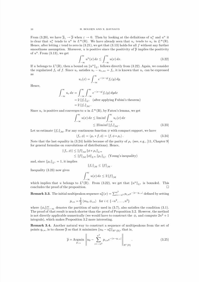
8/3/2019 Xavier Raynaud- On a Shallow Water Wave Equation
http://slidepdf.com/reader/full/xavier-raynaud-on-a-shallow-water-wave-equation 53/161
10 H. HOLDEN AND X. RAYNAUD
From (3.20), we have pε → p when ε → 0. Then by looking at the definitions of unε and un itis clear that unε tends to un in L∞(R). We have already seen that uε tends to uε in L∞(R).Hence, after letting ε tend to zero in (3.21), we get that (3.13) holds for all f without any further
smoothness assumption. Moreover, u is positive since the positivity of p implies the positivityof un. From (3.13), we get ∞
−∞
un(x) dx ≤ ∞−∞
u(x) dx. (3.22)
If u belongs to L1(R), then a bound on unL1 follows directly from (3.22). Again, we considerthe regularized f ε of f . Since uε satisfies uε − uε,xx = f ε, it is known that uε can be expressedas
uε(x) =
∞−∞
e−|x−y|f ε(y) dy.
Hence,
∞
−∞
uε dx =
∞
−∞ ∞
−∞
e−|x−y|f ε(y) dydx
= 2 f εL1 (after applying Fubini’s theorem)
= 2 f εM .
Since uε is positive and converges to u in L∞(R), by Fatou’s lemma, we get ∞−∞
u(x) dx ≤ lim inf
∞−∞
uε(x) dx
≤ 2liminf f εM . (3.23)
Let us estimate f εM. For any continuous function φ with compact support, we have
f ε, φ = ρε ∗ f, φ = f, φ ∗ ρε . (3.24)
Note that the last equality in (3.24) holds because of the parity of ρε (see, e.g., [11, Chapter 9]for general formulas on convolutions of distributions). Hence,
|f ε, φ| ≤ f M φ ∗ ρεL∞≤ f M φL∞ ρεL1 (Young’s inequality)
and, since ρεL1 = 1, it impliesf εM ≤ f M .
Inequality (3.23) now gives ∞−∞
u(x) dx ≤ 2 f Mwhich implies that u belongs to L1(R). From (3.22), we get that unL1 is bounded. Thisconcludes the proof of the proposition.
Remark 3.3. The initial multipeakon sequence un0 (x) =n2
i=−n2 pi,ne−|x−qi,n| defined by setting
pi,n =1
2m0, φi,n for i ∈ {−n2, . . . , n2}
where {φi}∞i=−∞ denotes the partition of unity used in (3.7), also satisfies the condition (3.1).The proof of that result is much shorter than the proof of Proposition 3.2. However, the methodis not directly applicable numerically (we would have to construct the φi and compute 2n2 + 1integrals), which makes Proposition 3.2 more interesting.
Remark 3.4. Another natural way to construct a sequence of multipeakons from the set of points qi,n, is to choose p so that it minimizes u0 − un0 H 1(R), that is,
p = Argmin pi,n
u0 −n2
i=−n2 pi,ne−|x−qi,n|
H 1(R)
. (3.25)
8/3/2019 Xavier Raynaud- On a Shallow Water Wave Equation
http://slidepdf.com/reader/full/xavier-raynaud-on-a-shallow-water-wave-equation 54/161
A NUMERICAL SCHEME BASED ON MULTIPEAKONS 11
It turns out that the sequence that this minimization method produces and the one of Proposition3.2 are the same. One can prove this as follows. We have
u0
−un
0 2
H 1
(R
)
=
u0
2
H 1
(R
) −2un
0
, u0
H 1 +
un
0 2
H 1
(R
)= u02
H 1(R) − 2
un0 − un0,xx, u0
M
+ 2 ptAp
and, since
un0 − un0,xx, u0
M
=
n2
i=−n2
2 pi,nδqi,n, u0
= 2
n2i=−n2
pi,nu0(qi,n) = 2 ptu,
we get
u0 − un0 2H 1(R) = u02
H 1(R) − 4 ptu + 2 ptAp. (3.26)
By differentiating (3.26) with respect to p, we can easily check that the minimizer p of (3.26)satisfies (3.3). In addition, since A is positive definite, p is the unique strict minimizer of (3.26).
The estimates contained in the following lemma will be needed to derive the existence of a
converging subsequence.
Lemma 3.5. Let un(x, t) be a sequence of multipeakons with initial data satisfying (3.1). The following properties hold:(i) un is uniformly bounded in H 1(R),(ii) unx is uniformly bounded in L∞(R),(iii) unx has a uniformly bounded total variation,(iv) unt is uniformly bounded in L2(R).
Proof. From Lemma 2.4 we know, using assumption (3.1c), that the system (2.10) has a uniqueglobal solution, and hence we have a globally defined sequence of multipeakons denoted un(x, t).In order to simplify the notation, we drop the superscript n on pni and qni and write
un =
ni=1
pie−|x−qi|.
Property (i) is obvious because of (3.1a) and the fact that the H 1 norm is automatically preserveddue to the Hamiltonian structure of (2.10). We have
unx(t, x) =ni=1
− pi(t)sgn(x − qi(t))e−|x−qi(t)| a.e.
Hence,
|unx(x, t)| ≤ni=1
pi(t)e−|x−qi(t)| ( pi ≥ 0)
≤ un
L∞
≤ C unH 1(R) (H 1(R) is continuously embedded in L∞(R))
and (ii) follows from (i). The total variation of unx equals unxxM (see, e.g., [10, Chapter 6]).We have
unxxM ≤ unM + un − unxxM . (3.27)
Since un ∈ L1(R), we have unM = unL1. At the same time, due to the positivity of the pi,the L1-norm of u is equal to M , the total mass of the system,
M =
un(x, t) dx = 2
ni=1
pi(t). (3.28)
As we have seen in the previous section, M is a conserved quantity. Hence,
M =
un
L1 =
un0
L1 .
8/3/2019 Xavier Raynaud- On a Shallow Water Wave Equation
http://slidepdf.com/reader/full/xavier-raynaud-on-a-shallow-water-wave-equation 55/161
12 H. HOLDEN AND X. RAYNAUD
Since the pi are positive, the fact that mn = un − unxx =n
i=1 2 piδqi and (3.28) imply that
un
−unxx
M = 2
n
i=1
pi = M. (3.29)
Hence, from (3.27),unxxM ≤ 2M = 2 un0 L1
and (iii) follows from (3.1b) .The derivative unt is given by
unt =
ni=1
˙ pie
−|x−qi| + piqi sgn(x − qi)e−|x−qi|
,
or, after using (2.10),
unt =n
i,j=1
pi pje−|x−qi|e−|qi−qj| (sgn(qi − qj) + sgn(x − qi)) .
Hence, since the pi are all positive,
unt L2 ≤ 2n
i,j=1
pi pje−|qi−qj|e−|x−qi|
L2
≤ 2n
i,j=1
pi pje−|qi−qj|
≤ un2H 1(R)
and assertion (iv) follows from (i).
To prove the existence of a converging subsequence of un in C ([0, T ], H 1loc(R)) we recall thefollowing compactness theorem adapted from Simon [18, Corollary 4].
Theorem 3.6 (Simon). Let X,B,Y be three continuously embedded Banach spaces
X ⊂ B ⊂ Y
with the first inclusion, X ⊂ B, compact. We consider a set F of continuous functions map-
ping [0, T ] into X . If F is bounded in L∞([0, T ], X ) and ∂ F ∂t =∂f ∂t | f ∈ F
is bounded in
Lr([0, T ], Y ) where r > 1, then F is relatively compact in C ([0, T ], B).
Proof of Theorem 3.1. Given initial data u0 ∈ H 1(R) with u0 − u0,xx ∈ M+ we know fromProposition 3.2 that there exists a sequence un0 satisfying condition (3.1). Furthermore, by usingLemma 2.4, we infer that there exists a sequence of multipeakons un(x, t) such that un|t=0 = un0 .The sequence then possesses the properties stated in Lemma 3.5.
To apply Theorem 3.6, we have to determine the Banach spaces with the required properties.
Let K be a compact subset of R. We define X = X (K ) as the set of functions of H 1
(K ) whichhave derivatives of bounded variation, that is,
X (K ) =
v ∈ H 1(K ) | vx ∈ BV (K )
endowed with the norm
vX(K) = vH 1(K) + vxBV (K) = vH 1(K) + vxL∞(K) + TVK(vx).
It follows that X (K ) is a Banach space. Let us prove that the injection X (K ) ⊂ H 1(K ) iscompact. We consider a sequence vn which is bounded in X (K ). By the Rellich–Kondrachovtheorem, since vnH 1(K) is bounded, there exists a subsequence (that we still denote vn) which
converges to some v in L2(R). Since TVK(vn,x) is bounded, Helly’s theorem allow us to extractanother subsequence such that
vn,x→
w a.e. in K (3.30)
8/3/2019 Xavier Raynaud- On a Shallow Water Wave Equation
http://slidepdf.com/reader/full/xavier-raynaud-on-a-shallow-water-wave-equation 56/161
A NUMERICAL SCHEME BASED ON MULTIPEAKONS 13
for some w ∈ L∞(K ). We have vn,xL∞(K) bounded. From (3.30) we get, by Lebesgue’s
dominated convergence theorem, that vn,x → w in L2(K ). Using the distributional definition of a derivative, it is not hard to check that w must coincide with vx. Therefore vn converges to v
in H 1(K ) and X (K ) is compactly embedded in H 1(K ).The estimates we have derived previously imply that un and unt are uniformly bounded in
L∞([0, T ], X (K )) and L∞([0, T ], L2(K )), respectively. Since X (K ) ⊂ H 1(K ) ⊂ L2(K ) withthe first inclusion compact, Simon’s theorem gives us the existence of a subsequence of un thatconverges to some u ∈ H 1(K ) in C ([0, T ], H 1(K )). We consider a sequence of compact setsK m such that R = ∪m∈NK m and a sequence of time T m such that limm→∞ T m = ∞. By adiagonal argument, we can find a subsequence (that we still denote un) that converges to someu ∈ C ([0, T m], H 1(K m)) in L∞([0, T m], H 1(K m)) for all m. Therefore u belongs to C (R, H 1loc(R))and un converges to u in L∞loc(R, H 1loc(R)).
It remains to prove that u is solution of the Camassa–Holm equation. This simply comesfrom the fact that the un are all weak solutions of (2.2), and since they converge to u inL∞loc(R, H 1loc(R)), u is a weak solution of (2.2). The solutions of the Camassa–Holm equation for
the class of initial data we are considering in the theorem are unique, see [8]. It implies that notonly a subsequence, but the whole sequence of multipeakons converges to the solution.
4. Numerical results
Multipeakons can be used in a numerical scheme to solve the Camassa–Holm equation withinitial data satisfying u0 − u0,xx ∈ M+. The scheme consists of solving the system of ordinarydifferential equations (2.10) where the initial conditions are computed as in Proposition 3.2.
In the numerical experiments that follow, we solve (2.10) by using the explicit Runge–Kuttasolver ode45 for ordinary differential equation from Matlab. In the case where u0 is sufficientlysmooth, an initial multipeakon sequence can be obtained without having to solve (3.2). This isthe aim of the following proposition.
Proposition 4.1. Let u0 be such that u0
−u0,xx is a positive function in H 1(R)
∩L1(R). We
set qi,n =
i
n,
pi,n =1
2n[u0 − u0,xx](qi,n) =
1
2nm0(qi,n).
(4.1)
Then the sequence un0 =n2
i=−n2 pi,ne−|x−qi,n| of multipeakons satisfies the conditions given in (3.1).
Proof. Condition (3.1c) follows directly from the definition of pi,n and the positivite of m0. Letus prove (3.1a), i.e., that un0 → u0 in H 1(R). It is enough to show that mn
0 tends to m0 in H −1
because the mapping v → v − vxx is an homeomorphism from H 1 to H −1 (see [2, chapter 8]).For any function φ in H 1(R), we have to prove that
mn0 , φ =
n2i=−n2
2 pi,nφ(qi,n) = 1n
n2i=−n2
m0(qi,n)φ(qi,n)
converges to
m0, φ =
R
m0(x)φ(x) dx.
If φ is continuous with compact support, the above convergence simply follows from the fact thatfor continuous functions, the Riemann sums converge to the integral. To prove that mn
0 , φ →m0, φ for any φ ∈ H 1(R), it is then enough to show that mn
0 H −1 is uniformly bounded. Infact, mn
0 is uniformly bounded in M and
mn0 M =
1
n
n2
i=−n2m0(qi,n) → m0L1 . (4.2)
8/3/2019 Xavier Raynaud- On a Shallow Water Wave Equation
http://slidepdf.com/reader/full/xavier-raynaud-on-a-shallow-water-wave-equation 57/161
14 H. HOLDEN AND X. RAYNAUD
Let us prove (4.2). We have
R
m0(x) dx = −n
−∞
m0(x) dx + n+ 1
n
−n
m0(x) dx + ∞
n+ 1n
m0(x) dx.
The first and the last integral tend to zero because m0 belongs to L1(R). Then we have n+ 1
n
−n
m0(x) dx − 1
n
n2i=−n2
m0(qi,n)
≤n2
i=−n2
qi+1,nqi,n
|m0(x) − m0(qi,n)| dx
≤n2
i=−n2
qi+1,nqi,n
xqi,n
|m0(ξ)| dξdx.
We change the order of integration, introduce χi,n to denote the characteristic function of theinterval (qi,n, qi+1,n), and get
n+ 1
n
−n
m0(x) dx − 1n
n2i=−n2
m0(qi,n) ≤ n2
i=−n2
qi+1
,n
qi,n
qi+1
,n
ξ
|m0(ξ)| dxdξ
=
∞−∞
|m0(ξ)|
n2i=−n2
χi,n(ξ)(qi+1,n − ξ) dξ
≤ m0L2
∞−∞
n2i=−n2
χi,n(ξ)(qi+1,n − ξ)2
dξ1/2
≤ m0H 1(R)
∞−∞
n2i=−n2
χi,n(ξ)(qi+1,n − ξ)2 dξ1/2
≤ m0H 1(R)
n
2i=−n2
qi+1,n
qi,n
(qi+1,n − ξ)2 dξ
1/2
≤ m0H 1(R)
n2i=−n2
1
3n3
1/2
≤ 1√n
m0H 1(R)
which tends to zero. This concludes the proof of (3.1a) and condition (3.1b) follows from (4.2)since we have, see (3.29),
un0 L1 = 2
n
i=1
pi = mn0 M .
We tested our algorithm with smooth traveling waves. Smooth traveling waves are solutionsof the form
u(x, t) = f (x − ct)
where f is solution of the second-order ordinary differential equation
f xx = f − α
(f − c)2. (4.3)
In order to give rise to a smooth traveling wave, the constants c and α cannot be chosen arbitrarily,see [15]. Here we consider periodic smooth traveling waves. The approach, based on functionsin H 1(R), which was developed in the previous sections, can be adapted to handle solutions
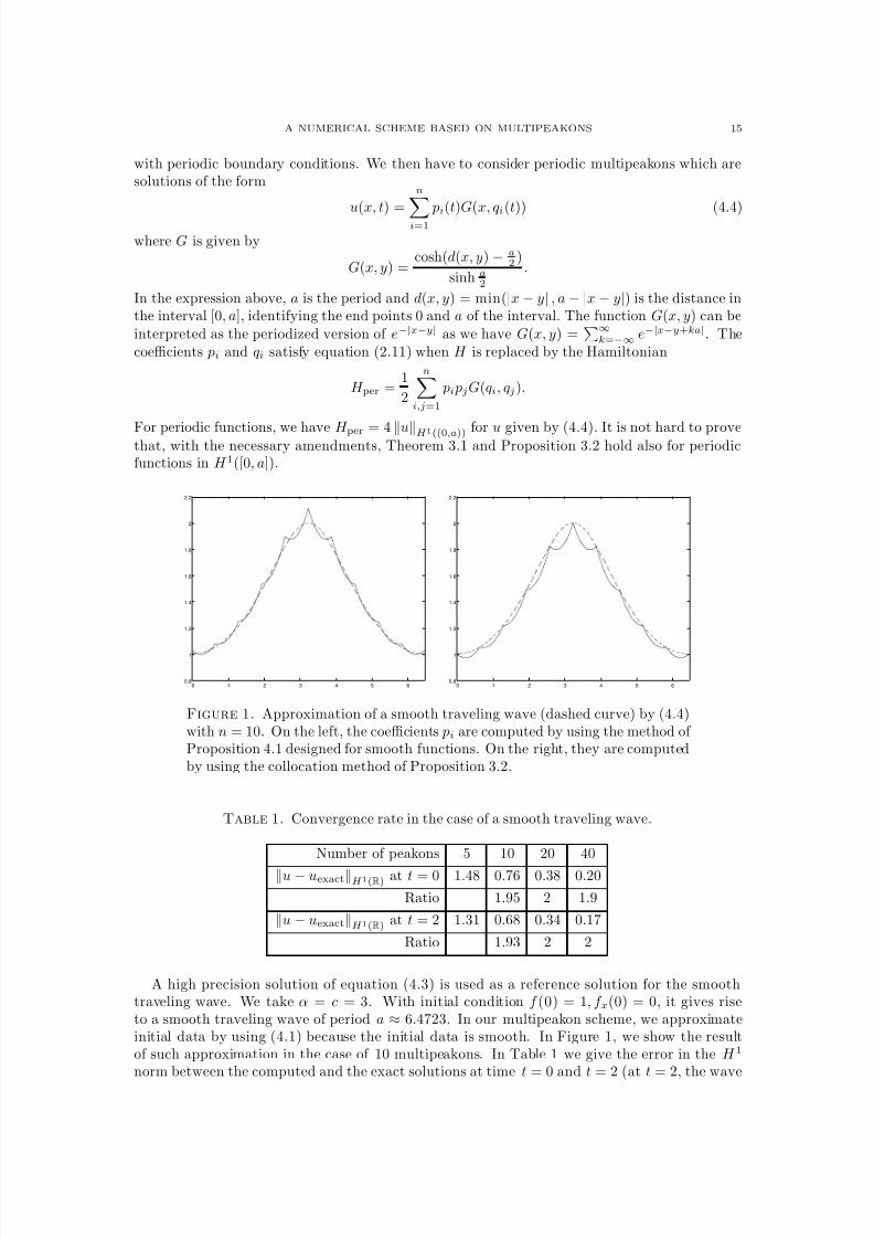
8/3/2019 Xavier Raynaud- On a Shallow Water Wave Equation
http://slidepdf.com/reader/full/xavier-raynaud-on-a-shallow-water-wave-equation 58/161
A NUMERICAL SCHEME BASED ON MULTIPEAKONS 15
with periodic boundary conditions. We then have to consider periodic multipeakons which aresolutions of the form
u(x, t) =n
i=1
pi(t)G(x, qi(t)) (4.4)
where G is given by
G(x, y) =cosh(d(x, y) − a
2 )
sinh a2
.
In the expression above, a is the period and d(x, y) = min(|x − y| , a − |x − y|) is the distance inthe interval [0, a], identifying the end points 0 and a of the interval. The function G(x, y) can beinterpreted as the periodized version of e−|x−y| as we have G(x, y) =
∞k=−∞ e−|x−y+ka|. The
coefficients pi and qi satisfy equation (2.11) when H is replaced by the Hamiltonian
H per =1
2
ni,j=1
pi pjG(qi, qj).
For periodic functions, we have H per = 4 uH 1((0,a)) for u given by (4.4). It is not hard to provethat, with the necessary amendments, Theorem 3.1 and Proposition 3.2 hold also for periodicfunctions in H 1([0, a]).
0 1 2 3 4 5 60.8
1
1.2
1.4
1.6
1.8
2
2.2
0 1 2 3 4 5 60.8
1
1.2
1.4
1.6
1.8
2
2.2
Figure 1. Approximation of a smooth traveling wave (dashed curve) by (4.4)with n = 10. On the left, the coefficients pi are computed by using the method of Proposition 4.1 designed for smooth functions. On the right, they are computedby using the collocation method of Proposition 3.2.
Table 1. Convergence rate in the case of a smooth traveling wave.
Number of peakons 5 10 20 40
u − uexactH 1(R) at t = 0 1.48 0.76 0.38 0.20
Ratio 1.95 2 1.9
u − uexactH 1(R) at t = 2 1.31 0.68 0.34 0.17
Ratio 1.93 2 2
A high precision solution of equation (4.3) is used as a reference solution for the smoothtraveling wave. We take α = c = 3. With initial condition f (0) = 1, f x(0) = 0, it gives riseto a smooth traveling wave of period a ≈ 6.4723. In our multipeakon scheme, we approximateinitial data by using (4.1) because the initial data is smooth. In Figure 1, we show the resultof such approximation in the case of 10 multipeakons. In Table 1 we give the error in the H 1
norm between the computed and the exact solutions at time t = 0 and t = 2 (at t = 2, the wave
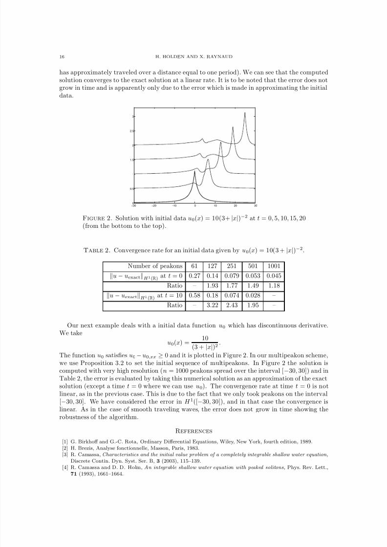
8/3/2019 Xavier Raynaud- On a Shallow Water Wave Equation
http://slidepdf.com/reader/full/xavier-raynaud-on-a-shallow-water-wave-equation 59/161
16 H. HOLDEN AND X. RAYNAUD
has approximately traveled over a distance equal to one period). We can see that the computedsolution converges to the exact solution at a linear rate. It is to be noted that the error does notgrow in time and is apparently only due to the error which is made in approximating the initial
data.
−30 −20 −10 0 10 20 300
0.5
1
1.5
2
2.5
3
Figure 2. Solution with initial data u0(x) = 10(3+ |x|)−2 at t = 0, 5, 10, 15, 20(from the bottom to the top).
Table 2. Convergence rate for an initial data given by u0(x) = 10(3 + |x|)−2.
Number of peakons 61 127 251 501 1001
u − uexactH 1(R) at t = 0 0.27 0.14 0.079 0.053 0.045
Ratio – 1.93 1.77 1.49 1.18u − uexactH 1(R) at t = 10 0.58 0.18 0.074 0.028 –
Ratio – 3.22 2.43 1.95 –
Our next example deals with a initial data function u0 which has discontinuous derivative.We take
u0(x) =10
(3 + |x|)2.
The function u0 satisfies u0 − u0,xx ≥ 0 and it is plotted in Figure 2. In our multipeakon scheme,we use Proposition 3.2 to set the initial sequence of multipeakons. In Figure 2 the solution iscomputed with very high resolution (n = 1000 peakons spread over the interval [−30, 30]) and inTable 2, the error is evaluated by taking this numerical solution as an approximation of the exactsolution (except a time t = 0 where we can use u0). The convergence rate at time t = 0 is notlinear, as in the previous case. This is due to the fact that we only took peakons on the interval[−30, 30]. We have considered the error in H 1([−30, 30]), and in that case the convergence islinear. As in the case of smooth traveling waves, the error does not grow in time showing therobustness of the algorithm.
References
[1] G. Birkhoff and G.-C. Rota, Ordinary Differential Equations, Wiley, New York, fourth edition, 1989.[2] H. Brezis, Analyse fonctionnelle, Masson, Paris, 1983.[3] R. Camassa, Characteristics and the initial value problem of a completely integrable shallow water equation,
Discrete Contin. Dyn. Syst. Ser. B, 3 (2003), 115–139.[4] R. Camassa and D. D. Holm, An integrable shallow water equation with peaked solitons, Phys. Rev. Lett.,
71 (1993), 1661–1664.
8/3/2019 Xavier Raynaud- On a Shallow Water Wave Equation
http://slidepdf.com/reader/full/xavier-raynaud-on-a-shallow-water-wave-equation 60/161
A NUMERICAL SCHEME BASED ON MULTIPEAKONS 17
[5] R. Camassa and D. D. Holm, and J. Hyman, A new integrable shallow water equation, Adv. Appl. Mech.,31 (1994), 1–33.
[6] R. Camassa, J. Huang, and L. Lee, Integral and integrable algorithms for a nonlinear shallow-water wave
equation, Preprint Submitted (2004).[7] R. Camassa, J. Huang, and L. Lee, On a completely integrable numerical scheme for a nonlinear shallow-
water equation, Preprint Submitted (2004).[8] A. Constantin and J. Escher, Global existence and blow-up for a shallow water equation, Ann. Scuola Norm.
Sup. Pisa Cl. Sci. (4), 26 (1998), 303–328.[9] A. Constantin and L. Molinet, Global weak solutions for a shallow water equation, Comm. Math. Phys., 211
(2000), 45–61.[10] L. C. Evans and R. F. Gariepy, Measure Theory and Fine Properties of Functions, CRC Press, Boca Raton,
FL, 1992.[11] G. B. Folland, Real Analysis, Wiley, New York, second edition, 1999.[12] A. A. Himonas and G. Misiolek, The Cauchy problem for an integrable shallow-water equation, Differential
Integral Equations, 14 (2001), 821–831.[13] H. Holden and X. Raynaud, Convergence of a finite difference scheme for the Camassa–Holm equation,
SIAM J. Numer. Anal. 2006, to appear. paper I in this thesis.[14] R. S. Johnson, Camassa–Holm, Korteweg–de Vries and related models for water, J. Fluid Mech, 455 (2002),
63–82.[15] H. Kalisch, Stability of solitary waves for a nonlinearly dispersive equation, Discrete Contin. Dyn. Syst., 10
(2004), 709–717.[16] Yi A. Li and P. J. Olver, Well-posedness and blow-up solutions for an integrable nonlinearly dispersive model
wave equation, J. Differential Equations, 162 (2000), 27–63.[17] G. Rodrıguez-Blanco, On the Cauchy problem for the Camassa–Holm equation, Nonlinear Anal., 46 (2001),
309–327.[18] J. Simon, Compact sets in the space Lp(0, T ;B), Ann. Mat. Pura Appl. (4), 146 (1987), 65–96.
8/3/2019 Xavier Raynaud- On a Shallow Water Wave Equation
http://slidepdf.com/reader/full/xavier-raynaud-on-a-shallow-water-wave-equation 61/161
Paper III
Convergence of a Spectral Projectionof the Camassa-Holm equation.
H. Kalisch and X. RaynaudTo appear in Numerical Methods for Partial Differential Equations.

8/3/2019 Xavier Raynaud- On a Shallow Water Wave Equation
http://slidepdf.com/reader/full/xavier-raynaud-on-a-shallow-water-wave-equation 62/161
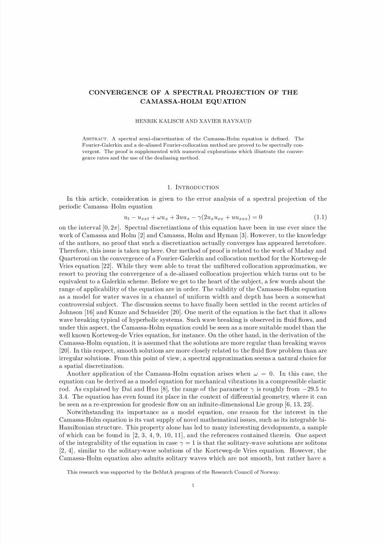
8/3/2019 Xavier Raynaud- On a Shallow Water Wave Equation
http://slidepdf.com/reader/full/xavier-raynaud-on-a-shallow-water-wave-equation 63/161
CONVERGENCE OF A SPECTRAL PROJECTION OF THECAMASSA-HOLM EQUATION
HENRIK KALISCH AND XAVIER RAYNAUD
Abstract. A spectral semi-discretization of the Camassa-Holm equation is defined. TheFourier-Galerkin and a de-aliased Fourier-collocation method are proved to be spectrally con-vergent. The proof is supplemented with numerical explorations which illustrate the conver-gence rates and the use of the dealiasing method.
1. Introduction
In this article, consideration is given to the error analysis of a spectral projection of theperiodic Camassa–Holm equation
ut − uxxt + ωux + 3uux − γ (2uxuxx + uuxxx) = 0 (1.1)
on the interval [0, 2π]. Spectral discretizations of this equation have been in use ever since thework of Camassa and Holm [2] and Camassa, Holm and Hyman [3]. However, to the knowledgeof the authors, no proof that such a discretization actually converges has appeared heretofore.Therefore, this issue is taken up here. Our method of proof is related to the work of Maday andQuarteroni on the convergence of a Fourier-Galerkin and collocation method for the Korteweg-deVries equation [22]. While they were able to treat the unfiltered collocation approximation, weresort to proving the convergence of a de-aliased collocation projection which turns out to beequivalent to a Galerkin scheme. Before we get to the heart of the subject, a few words about therange of applicability of the equation are in order. The validity of the Camassa-Holm equationas a model for water waves in a channel of uniform width and depth has been a somewhatcontroversial subject. The discussion seems to have finally been settled in the recent articles of Johnson [16] and Kunze and Schneider [20]. One merit of the equation is the fact that it allowswave breaking typical of hyperbolic systems. Such wave breaking is observed in fluid flows, andunder this aspect, the Camassa-Holm equation could be seen as a more suitable model than thewell known Korteweg-de Vries equation, for instance. On the other hand, in the derivation of theCamassa-Holm equation, it is assumed that the solutions are more regular than breaking waves[20]. In this respect, smooth solutions are more closely related to the fluid flow problem than areirregular solutions. From this point of view, a spectral approximation seems a natural choice fora spatial discretization.
Another application of the Camassa-Holm equation arises when ω = 0. In this case, the
equation can be derived as a model equation for mechanical vibrations in a compressible elasticrod. As explained by Dai and Huo [8], the range of the parameter γ is roughly from −29.5 to3.4. The equation has even found its place in the context of differential geometry, where it canbe seen as a re-expression for geodesic flow on an infinite-dimensional Lie group [6, 13, 23].
Notwithstanding its importance as a model equation, one reason for the interest in theCamassa-Holm equation is its vast supply of novel mathematical issues, such as its integrable bi-Hamiltonian structure. This property alone has led to many interesting developments, a sampleof which can be found in [2, 3, 4, 9, 10, 11], and the references contained therein. One aspectof the integrability of the equation in case γ = 1 is that the solitary-wave solutions are solitons[2, 4], similar to the solitary-wave solutions of the Korteweg-de Vries equation. However, theCamassa-Holm equation also admits solitary waves which are not smooth, but rather have a
This research was supported by the BeMatA program of the Research Council of Norway.
1
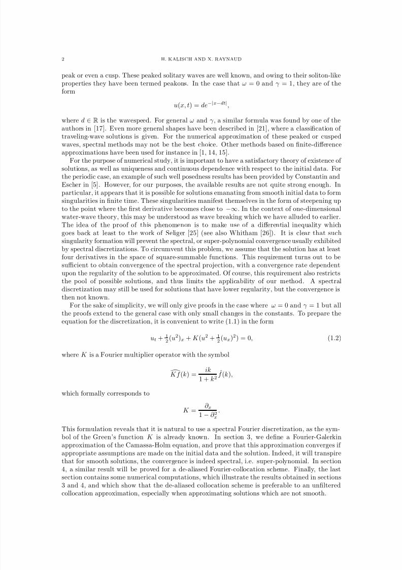
8/3/2019 Xavier Raynaud- On a Shallow Water Wave Equation
http://slidepdf.com/reader/full/xavier-raynaud-on-a-shallow-water-wave-equation 64/161
2 H. KALISCH AND X. RAYNAUD
peak or even a cusp. These peaked solitary waves are well known, and owing to their soliton-likeproperties they have been termed peakons. In the case that ω = 0 and γ = 1, they are of theform
u(x, t) = de−|x−dt|,
where d ∈ R is the wavespeed. For general ω and γ , a similar formula was found by one of theauthors in [17]. Even more general shapes have been described in [21], where a classification of traveling-wave solutions is given. For the numerical approximation of these peaked or cuspedwaves, spectral methods may not be the best choice. Other methods based on finite-differenceapproximations have been used for instance in [1, 14, 15].
For the purpose of numerical study, it is important to have a satisfactory theory of existence of solutions, as well as uniqueness and continuous dependence with respect to the initial data. Forthe periodic case, an example of such well posedness results has been provided by Constantin andEscher in [5]. However, for our purposes, the available results are not quite strong enough. Inparticular, it appears that it is possible for solutions emanating from smooth initial data to form
singularities in finite time. These singularities manifest themselves in the form of steepening upto the point where the first derivative becomes close to −∞. In the context of one-dimensionalwater-wave theory, this may be understood as wave breaking which we have alluded to earlier.The idea of the proof of this phenomenon is to make use of a differential inequality whichgoes back at least to the work of Seliger [25] (see also Whitham [26]). It is clear that suchsingularity formation will prevent the spectral, or super-polynomial convergence usually exhibitedby spectral discretizations. To circumvent this problem, we assume that the solution has at leastfour derivatives in the space of square-summable functions. This requirement turns out to besufficient to obtain convergence of the spectral projection, with a convergence rate dependentupon the regularity of the solution to be approximated. Of course, this requirement also restrictsthe pool of possible solutions, and thus limits the applicability of our method. A spectraldiscretization may still be used for solutions that have lower regularity, but the convergence is
then not known.For the sake of simplicity, we will only give proofs in the case where ω = 0 and γ = 1 but allthe proofs extend to the general case with only small changes in the constants. To prepare theequation for the discretization, it is convenient to write (1.1) in the form
ut + 12
(u2)x + K (u2 + 12
(ux)2) = 0, (1.2)
where K is a Fourier multiplier operator with the symbol
Kf (k) =ik
1 + k2f (k),
which formally corresponds to
K =∂ x
1 − ∂ 2x.
This formulation reveals that it is natural to use a spectral Fourier discretization, as the sym-bol of the Green’s function K is already known. In section 3, we define a Fourier-Galerkinapproximation of the Camassa-Holm equation, and prove that this approximation converges if appropriate assumptions are made on the initial data and the solution. Indeed, it will transpirethat for smooth solutions, the convergence is indeed spectral, i.e. super-polynomial. In section4, a similar result will be proved for a de-aliased Fourier-collocation scheme. Finally, the lastsection contains some numerical computations, which illustrate the results obtained in sections3 and 4, and which show that the de-aliased collocation scheme is preferable to an unfilteredcollocation approximation, especially when approximating solutions which are not smooth.
8/3/2019 Xavier Raynaud- On a Shallow Water Wave Equation
http://slidepdf.com/reader/full/xavier-raynaud-on-a-shallow-water-wave-equation 65/161
SPECTRAL PROJECTION OF THE CAMASSA-HOLM EQUATION 3
2. Notation
In order to facilitate our study, we start by introducing some mathematical notation. Denotethe inner product in L2(0, 2π) by
(f, g) = 2π
0
f (x) g(x) dx.
The Fourier coefficients f (k) of a function f ∈ L2(0, 2π) are defined by
f (k) =1
2π
2π
0
e−ikxf (x) dx.
Recall the inversion formulaf (x) =
k∈Z
eikxf (k),
and the convolution formula(f ∗ g)(k) =
f g(k),
where the convolution of two functions f and g on Z is formally defined by
(f ∗ g)(k) =
m+n=k
f (m) g(n).
Denote by · H m the Sobolev norm, given by
f 2H m =
k∈Z
(1 + |k|2)m|f (k)|2.
The space of periodic Sobolev functions on the interval [0, 2π] is defined as the closure of thespace of smooth periodic functions with respect to the H m-norm, and will be simply denoted byH m. In particular, for m = 0, we recover the space L2(0, 2π) whose norm will be denoted by · L2. The subspace of L2(0, 2π) spanned by the set
eikx k ∈ Z, −
N
2 ≤ k ≤N
2 − 1for N even is denoted by S N . In the following, it will always be assumed that N is even. Theoperator P N denotes the orthogonal, self-adjoint, projection from L2 onto S N , defined by
P N f (x) =
−N/2≤k≤N/2−1
eikxf (k).
For f ∈ H m, the estimates
f − P N f L2 ≤ C P N −m ∂ mx f L2 , (2.1)
f − P N f H n ≤ C P N n−m ∂ mx f L2 (2.2)
hold for an appropriate constant C P and a positive integer n. For the proof of these inequalities,the reader is referred to [7].
The space of continuous functions from the interval [0, T ] into the space H n is denoted byC ([0, T ], H n). Similarly, we also consider the space C ([0, T ], S N ), where the topology on thefinite-dimensional space S N can be given by any norm. Finally note the inverse inequality
∂ mx φL2 ≤ N m φL2 , (2.3)
which holds for integers m > 0 and φ ∈ S N . A proof of this estimate can also be found in [7].We will make use of the Sobolev lemma, which guarantees the existence of a constant c, suchthat
supx
|f (x)| ≤ c f H 1 . (2.4)
Another standard result is that the assignment (f, g) → f g is a continuous bilinear map fromH 1 × H −1 to H −1, as shown by the estimate
f g
H −1
≤c
f
H 1
g
H −1 , (2.5)
8/3/2019 Xavier Raynaud- On a Shallow Water Wave Equation
http://slidepdf.com/reader/full/xavier-raynaud-on-a-shallow-water-wave-equation 66/161
4 H. KALISCH AND X. RAYNAUD
where the same constant c has been used for simplicity.In order to obtain a unique solution, equation (1.1) has to be supplemented by appropriate
boundary and initial conditions. For the purpose of numerical approximation, the problem will
be studied on a finite interval with periodic boundary conditions. The periodic initial valueproblem associated to equation (1.1) is
ut − uxxt + 3uux − 2uxuxx − uuxxx = 0 x ∈ [0, 2π] , t ≥ 0,
u(0, t) = u(2π, t), t ≥ 0,
u(x, 0) = u0(x).
(2.6)
In the following, it will always be assumed that a solution of this problem exists on some timeinterval [0, T ], and with a certain amount of spatial regularity. In particular, we suppose that asolution exists in the space C ([0, T ], H 4) for some T > 0. With these preliminaries in place, weare set to attack the problem of defining a suitable spectral projection of (2.6) and proving theconvergence of such a projection. First, the Fourier-Galerkin method is presented and a proof of convergence given. Then in section 4, a de-aliased collocation scheme will be treated.
3. The Fourier-Galerkin method.
A space-discretization of (2.6) is defined by utilizing the equivalent formulation (1.2). Thusthe problem is to find a function uN from [0, T ] to S N which satisfies
∂ tuN +12 ∂ x(uN )
2 + K
u2N +
12 (∂ xuN )
2
, φ
= 0, t ∈ [0, T ],
uN (0) = P N u0,(3.1)
for all φ ∈ S N . Since for each t, uN (·, t) ∈ S N , uN has the form
uN (x, t) =
N
2−1
k=−N2
uN (k, t)eikx,
where uN (k, t) are the Fourier coefficients of uN (·, t).Taking φ = eikx for −N/2 ≤ k ≤ N/2 − 1 in (3.1) yields the following system of equations for
the Fourier coefficients of uN .d
dtuN (k, t) = −1
2ik(uN ∗ uN )(k, t) − ik
1 + k2
(uN ∗ uN )(k, t)
+ 12
((ikuN ) ∗ (ikuN ))(k, t)
,
uN (k, 0) = u0(k),
(3.2)
for −N/2 ≤ k < N/2 − 1..The short-time existence of a maximal solution of (3.2) is proved using the contraction map-
ping principle, and the solution is unique on its maximal interval of definition, [0, tmN ), where tmN ispossibly equal to T . Since the argument is standard, the proof is omitted here. The main result
of this paper is the fact that the Galerkin approximation uN converges to the exact solution uwhen u is smooth enough. This is stated in the next theorem.
Theorem 3.1. Suppose that a solution u of the Camassa-Holm equation (2.6) exists in the space
C ([0, T ], H m) for m ≥ 4, and for some time T > 0. Then for N large enough, there exists a
unique solution uN of the finite-dimensional problem (3.1). Moreover, there exists a constant λsuch that
supt∈[0,T ]
u(·, t) − uN (·, t)L2 ≤ λN 1−m.
Before the proof is given, note that the assumptions of the theorem encompass the existenceof a constant κ, such that
supt∈[0,T ]
u(·, t)H m ≤ κ.
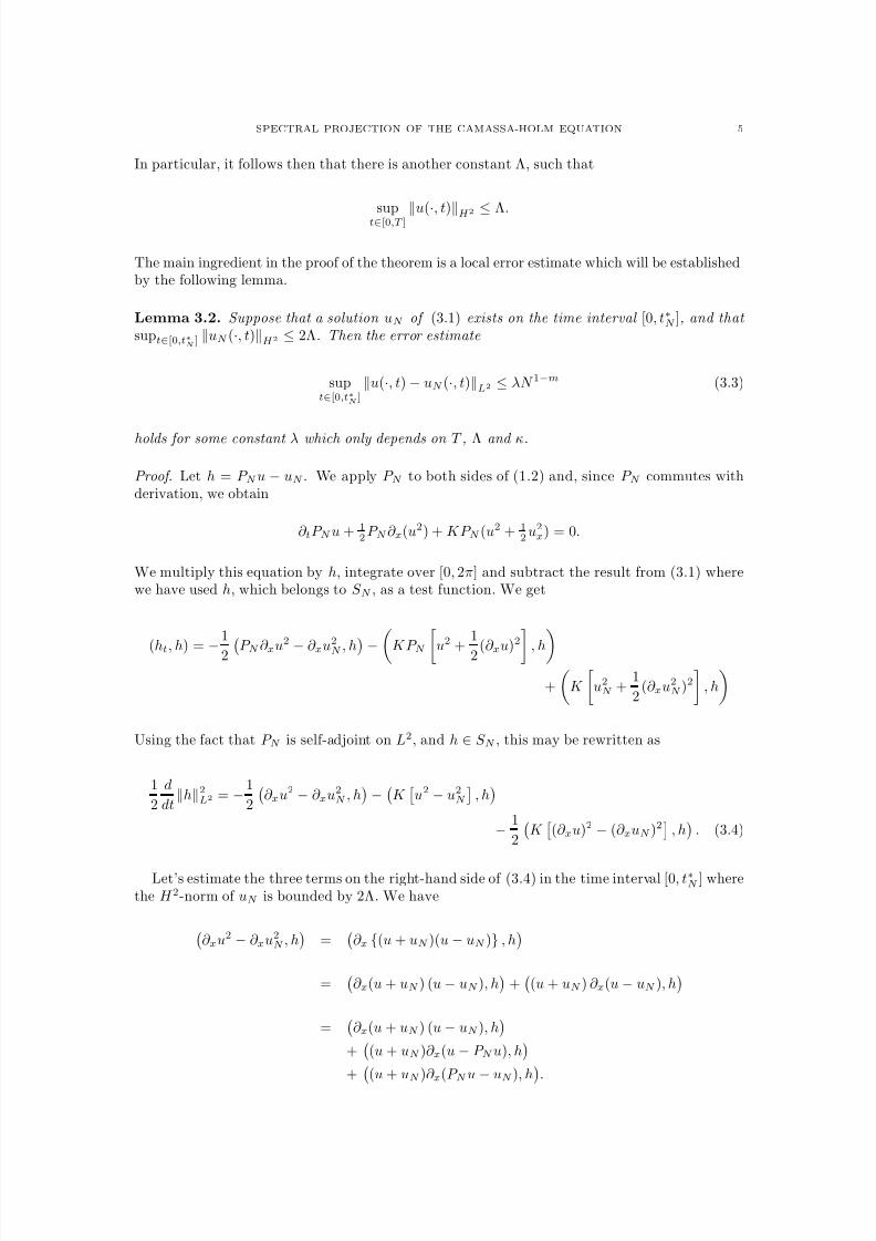
8/3/2019 Xavier Raynaud- On a Shallow Water Wave Equation
http://slidepdf.com/reader/full/xavier-raynaud-on-a-shallow-water-wave-equation 67/161
SPECTRAL PROJECTION OF THE CAMASSA-HOLM EQUATION 5
In particular, it follows then that there is another constant Λ, such that
supt∈[0,T ]
u(·, t)
H 2
≤Λ.
The main ingredient in the proof of the theorem is a local error estimate which will be establishedby the following lemma.
Lemma 3.2. Suppose that a solution uN of (3.1) exists on the time interval [0, t∗N ], and that
supt∈[0,t∗N
] uN (·, t)H 2 ≤ 2Λ. Then the error estimate
supt∈[0,t∗
N]
u(·, t) − uN (·, t)L2 ≤ λN 1−m (3.3)
holds for some constant λ which only depends on T , Λ and κ.
Proof. Let h = P N u − uN . We apply P N to both sides of (1.2) and, since P N commutes withderivation, we obtain
∂ tP N u + 12 P N ∂ x(u2) + KP N (u2 + 1
2 u2x) = 0.
We multiply this equation by h, integrate over [0, 2π] and subtract the result from (3.1) wherewe have used h, which belongs to S N , as a test function. We get
(ht, h) = −1
2 P N ∂ xu
2
− ∂ xu
2
N , h−KP N u
2
+
1
2 (∂ xu)
2 , h+
K
u2N +
1
2(∂ xu2
N )2
, h
Using the fact that P N is self-adjoint on L2, and h ∈ S N , this may be rewritten as
1
2
d
dth2
L2 = − 1
2
∂ xu2 − ∂ xu2
N , h−
K
u2 − u2N
, h− 1
2
K
(∂ xu)2 − (∂ xuN )2
, h
. (3.4)
Let’s estimate the three terms on the right-hand side of (3.4) in the time interval [0, t∗N ] wherethe H 2-norm of uN is bounded by 2Λ. We have
∂ xu2 − ∂ xu2
N , h
=
∂ x {(u + uN )(u − uN )} , h
=
∂ x(u + uN ) (u − uN ), h
+
(u + uN ) ∂ x(u − uN ), h
=
∂ x(u + uN ) (u − uN ), h
+
(u + uN )∂ x(u − P N u), h
+ (u + uN )∂ x(P N u
−uN ), h.
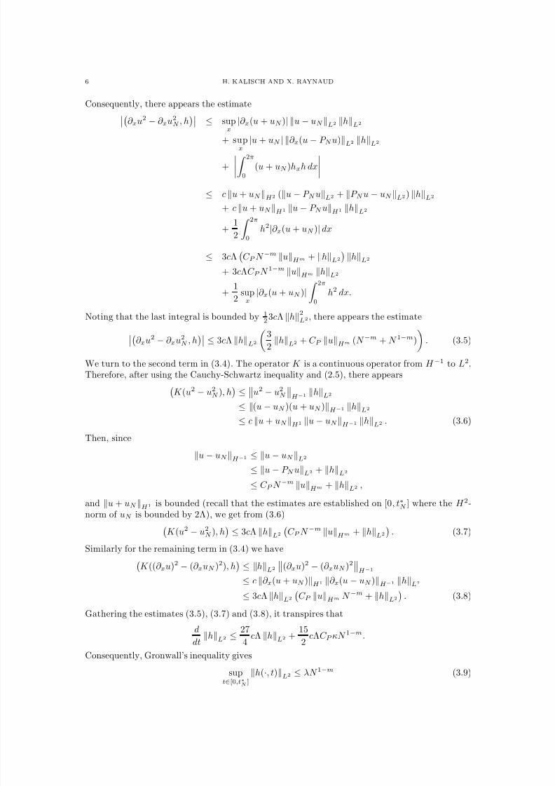
8/3/2019 Xavier Raynaud- On a Shallow Water Wave Equation
http://slidepdf.com/reader/full/xavier-raynaud-on-a-shallow-water-wave-equation 68/161
6 H. KALISCH AND X. RAYNAUD
Consequently, there appears the estimate
∂ xu2 − ∂ xu2
N , h
≤ sup
x|∂ x(u + uN )| u − uN L2 hL2
+ supx
|u + uN | ∂ x(u − P N u)L2 hL2
+
2π
0
(u + uN )hxh dx
≤ c u + uN H 2 (u − P N uL2 + P N u − uN L2) hL2
+ c u + uN H 1 u − P N uH 1 hL2
+1
2
2π
0
h2|∂ x(u + uN )| dx
≤ 3cΛ
C P N −m uH m + hL2
hL2
+ 3cΛC P N
1−m
uH m hL2
+1
2supx
|∂ x(u + uN )| 2π
0
h2 dx.
Noting that the last integral is bounded by 12 3cΛ h2
L2, there appears the estimate∂ xu2 − ∂ xu2N , h
≤ 3cΛ hL2
3
2hL2 + C P uH m (N −m + N 1−m)
. (3.5)
We turn to the second term in (3.4). The operator K is a continuous operator from H −1 to L2.Therefore, after using the Cauchy-Schwartz inequality and (2.5), there appears
K (u2 − u2
N ), h
≤
u2 − u2
N
H −1
hL2
≤ (u
−uN )(u + uN )
H −1
hL
2
≤ c u + uN H 1 u − uN H −1 hL2 . (3.6)
Then, since
u − uN H −1 ≤ u − uN L2
≤ u − P N uL2 + hL2
≤ C P N −m uH m + hL2 ,
and u + uN H 1 is bounded (recall that the estimates are established on [0, t∗N ] where the H 2-norm of uN is bounded by 2Λ), we get from (3.6)
K (u2 − u2
N ), h
≤ 3cΛ hL2
C P N −m uH m + hL2
. (3.7)
Similarly for the remaining term in (3.4) we haveK ((∂ xu)2 − (∂ xuN )
2), h ≤ hL2
(∂ xu)2 − (∂ xuN )2H −1
≤ c ∂ x(u + uN )H 1 ∂ x(u − uN )H −1 hL2
≤ 3cΛ hL2
C P uH m N −m + hL2
. (3.8)
Gathering the estimates (3.5), (3.7) and (3.8), it transpires that
d
dthL2 ≤ 27
4cΛ hL2 +
15
2cΛC P κN 1−m.
Consequently, Gronwall’s inequality gives
supt∈[0,t∗
N]
h(·, t)L2 ≤ λN 1−m (3.9)
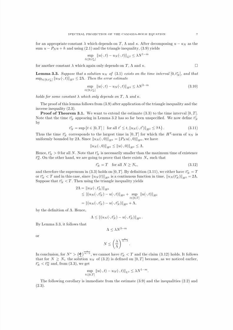
8/3/2019 Xavier Raynaud- On a Shallow Water Wave Equation
http://slidepdf.com/reader/full/xavier-raynaud-on-a-shallow-water-wave-equation 69/161
SPECTRAL PROJECTION OF THE CAMASSA-HOLM EQUATION 7
for an appropriate constant λ which depends on T , Λ and κ. After decomposing u − uN as thesum u − P N u + h and using (2.1) and the triangle inequality, (3.9) yields
supt∈[0,t∗
N]
u(·, t)
−uN (
·, t)
L2
≤λN 1−m
for another constant λ which again only depends on T , Λ and κ.
Lemma 3.3. Suppose that a solution uN of (3.1) exists on the time interval [0, t∗N ], and that
supt∈[0,t∗N
] uN (·, t)H 2 ≤ 2Λ. Then the error estimate
supt∈[0,t∗
N]
u(·, t) − uN (·, t)H 2 ≤ λN 3−m (3.10)
holds for some constant λ which only depends on T , Λ and κ.
The proof of this lemma follows from (3.9) after application of the triangle inequality and theinverse inequality (2.3).
Proof of Theorem 3.1. We want to extend the estimate (3.3) to the time interval [0 , T ].Note that the time t∗N appearing in Lemma 3.2 has so far been unspecified. We now define t∗N by
t∗N = sup {t ∈ [0, T ] | for all t ≤ t, uN (·, t)H 2 ≤ 2Λ} . (3.11)
Thus the time t∗N corresponds to the largest time in [0, T ] for which the H 2-norm of uN isuniformly bounded by 2Λ. Since uN (·, 0)H 2 = P N u(·, 0)H 2 , we have
uN (·, 0)H 2 ≤ u(·, 0)H 2 ≤ Λ.
Hence, t∗N > 0 for all N . Note that t∗N is necessarily smaller than the maximum time of existencetmN . On the other hand, we are going to prove that there exists N ∗ such that
t∗N = T for all N ≥ N ∗, (3.12)
and therefore the supremum in (3.3) holds on [0, T ]. By definition (3.11), we either have t
∗
N = T or t∗N < T and in this case, since uN (t)H 2 is a continuous function in time, uN (t∗N )H 2 = 2Λ.Suppose that t∗N < T . Then using the triangle inequality yields
2Λ = uN (·, t∗N )H 2≤ (uN (·, t∗N ) − u(·, t)H 2 + sup
t∈[0,T ]
u(·, t)H 2
= (uN (·, t∗N ) − u(·, t∗N )H 2 + Λ,
by the definition of Λ. Hence,
Λ ≤ (uN (·, t∗N ) − u(·, t∗N )H 2 .
By Lemma 3.3, it follows that
Λ ≤ λN
3−m
or
N ≤
λ
Λ
1
m−3
.
In conclusion, for N ∗ >λΛ
1
m−3 , we cannot have t∗N < T and the claim (3.12) holds. It followsthat for N ≥ N ∗ the solution uN of (3.2) is defined on [0, T ] because, as we noticed earlier,t∗N < tmN and, from (3.3), we get
supt∈[0,T ]
u(·, t) − uN (·, t)L2 ≤ λN 1−m.
The following corollary is immediate from the estimate (3.9) and the inequalities (2.2) and(2.3).
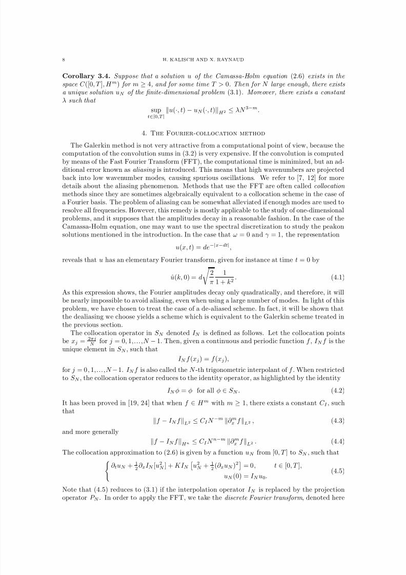
8/3/2019 Xavier Raynaud- On a Shallow Water Wave Equation
http://slidepdf.com/reader/full/xavier-raynaud-on-a-shallow-water-wave-equation 70/161
8 H. KALISCH AND X. RAYNAUD
Corollary 3.4. Suppose that a solution u of the Camassa-Holm equation (2.6) exists in the
space C ([0, T ], H m) for m ≥ 4, and for some time T > 0. Then for N large enough, there exists
a unique solution uN of the finite-dimensional problem (3.1). Moreover, there exists a constant
λ such that sup
t∈[0,T ]
u(·, t) − uN (·, t)H 2 ≤ λN 3−m.
4. The Fourier-collocation method
The Galerkin method is not very attractive from a computational point of view, because thecomputation of the convolution sums in (3.2) is very expensive. If the convolution is computedby means of the Fast Fourier Transform (FFT), the computational time is minimized, but an ad-ditional error known as aliasing is introduced. This means that high wavenumbers are projectedback into low wavenumber modes, causing spurious oscillations. We refer to [7, 12] for moredetails about the aliasing phenomenon. Methods that use the FFT are often called collocation
methods since they are sometimes algebraically equivalent to a collocation scheme in the case of
a Fourier basis. The problem of aliasing can be somewhat alleviated if enough modes are used toresolve all frequencies. However, this remedy is mostly applicable to the study of one-dimensionalproblems, and it supposes that the amplitudes decay in a reasonable fashion. In the case of theCamassa-Holm equation, one may want to use the spectral discretization to study the peakonsolutions mentioned in the introduction. In the case that ω = 0 and γ = 1, the representation
u(x, t) = de−|x−dt|,
reveals that u has an elementary Fourier transform, given for instance at time t = 0 by
u(k, 0) = d
2
π
1
1 + k2. (4.1)
As this expression shows, the Fourier amplitudes decay only quadratically, and therefore, it will
be nearly impossible to avoid aliasing, even when using a large number of modes. In light of thisproblem, we have chosen to treat the case of a de-aliased scheme. In fact, it will be shown thatthe dealiasing we choose yields a scheme which is equivalent to the Galerkin scheme treated inthe previous section.
The collocation operator in S N denoted I N is defined as follows. Let the collocation pointsbe xj = 2πj
N for j = 0, 1,...,N − 1. Then, given a continuous and periodic function f , I N f is the
unique element in S N , such that
I N f (xj) = f (xj),
for j = 0, 1,...,N −1. I N f is also called the N -th trigonometric interpolant of f . When restrictedto S N , the collocation operator reduces to the identity operator, as highlighted by the identity
I N φ = φ for all φ ∈ S N . (4.2)
It has been proved in [19, 24] that when f ∈ H m with m ≥ 1, there exists a constant C I , suchthat
f − I N f L2 ≤ C I N −m ∂ mx f L2 , (4.3)
and more generally
f − I N f H n ≤ C I N n−m ∂ mx f L2 . (4.4)
The collocation approximation to (2.6) is given by a function uN from [0, T ] to S N , such that∂ tuN +
12
∂ xI N [u2N ] + KI N
u2N +
12
(∂ xuN )2
= 0, t ∈ [0, T ],
uN (0) = I N u0.(4.5)
Note that (4.5) reduces to (3.1) if the interpolation operator I N is replaced by the projectionoperator P N . In order to apply the FFT, we take the discrete Fourier transform , denoted here
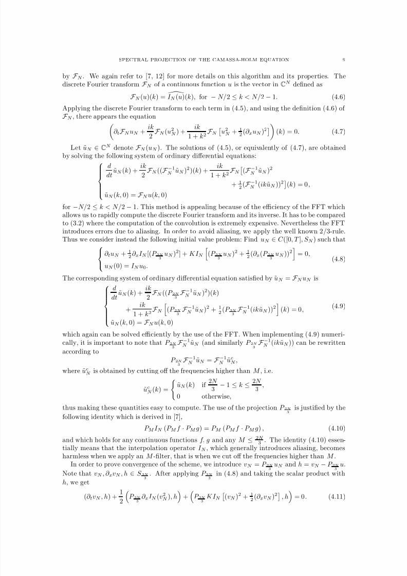
8/3/2019 Xavier Raynaud- On a Shallow Water Wave Equation
http://slidepdf.com/reader/full/xavier-raynaud-on-a-shallow-water-wave-equation 71/161
SPECTRAL PROJECTION OF THE CAMASSA-HOLM EQUATION 9
by F N . We again refer to [7, 12] for more details on this algorithm and its properties. Thediscrete Fourier transform F N of a continuous function u is the vector in CN defined as
F N (u)(k) = I
N (u)(k), for
−N/2
≤k < N/2
−1. (4.6)
Applying the discrete Fourier transform to each term in (4.5), and using the definition (4.6) of F N , there appears the equation
∂ tF N uN + ik
2F N (u2
N ) +ik
1 + k2F N
u2N +
12 (∂ xuN )
2
(k) = 0. (4.7)
Let uN ∈ CN denote F N (uN ). The solutions of (4.5), or equivalently of (4.7), are obtainedby solving the following system of ordinary differential equations:
d
dtuN (k) +
ik
2F N ((F −1
N uN )2)(k) +
ik
1 + k2F N
(F −1
N uN )2
+ 12 (F −1
N (ikuN ))2
(k) = 0,
uN (k, 0) =
F N u(k, 0)
for −N/2 ≤ k < N/2 − 1. This method is appealing because of the efficiency of the FFT whichallows us to rapidly compute the discrete Fourier transform and its inverse. It has to be comparedto (3.2) where the computation of the convolution is extremely expensive. Nevertheless the FFTintroduces errors due to aliasing. In order to avoid aliasing, we apply the well known 2/3-rule.Thus we consider instead the following initial value problem: Find uN ∈ C ([0, T ], S N ) such that ∂ tuN +
12 ∂ xI N [(P 2N
3
uN )2] + KI N
(P 2N
3
uN )2 + 1
2 (∂ x(P 2N3
uN ))2
= 0,
uN (0) = I N u0.(4.8)
The corresponding system of ordinary differential equation satisfied by uN = F N uN is
d
dtuN (k) +
ik
2F N ((P 2N
3
F −1N uN )
2)(k)
+ik
1 + k2F N (P 2N
3
F −1N uN )
2 + 12 (P 2N
3
F −1N (ikuN ))2 (k) = 0,
uN (k, 0) = F N u(k, 0)
(4.9)
which again can be solved efficiently by the use of the FFT. When implementing (4.9) numeri-cally, it is important to note that P 2N
3
F −1N uN (and similarly P 2N
3
F −1N (ikuN )) can be rewritten
according to
P 2N3
F −1N uN = F −1
N ucN ,
where ucN is obtained by cutting off the frequencies higher than M , i.e.
ucN (k) =
uN (k) if
2N
3− 1 ≤ k ≤ 2N
3,
0 otherwise,
thus making these quantities easy to compute. The use of the projection P 2N3
is justified by the
following identity which is derived in [7],
P M I N (P M f · P M g) = P M (P M f · P M g) , (4.10)
and which holds for any continuous functions f, g and any M ≤ 2N 3 . The identity (4.10) essen-
tially means that the interpolation operator I N , which generally introduces aliasing, becomesharmless when we apply an M -filter, that is when we cut off the frequencies higher than M .
In order to prove convergence of the scheme, we introduce vN = P 2N3
uN and h = vN − P 2N3
u.
Note that vN , ∂ xvN , h ∈ S 2N3
. After applying P 2N3
in (4.8) and taking the scalar product with
h, we get
(∂ tvN , h) +1
2 P 2N3
∂ xI N (v2N ), h+ P 2N
3
KI N (vN )2 + 1
2 (∂ xvN )2
, h = 0. (4.11)
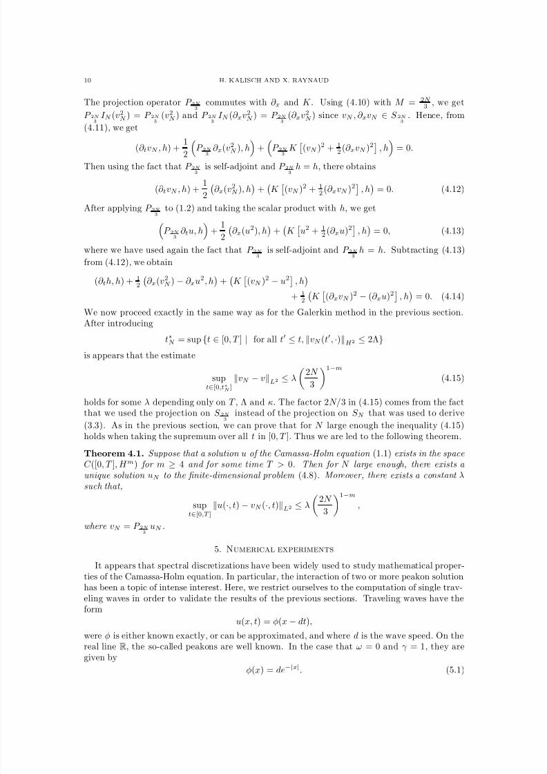
8/3/2019 Xavier Raynaud- On a Shallow Water Wave Equation
http://slidepdf.com/reader/full/xavier-raynaud-on-a-shallow-water-wave-equation 72/161
10 H. KALISCH AND X. RAYNAUD
The projection operator P 2N3
commutes with ∂ x and K . Using (4.10) with M = 2N 3 , we get
P 2N3
I N (v2N ) = P 2N
3
(v2N ) and P 2N
3
I N (∂ xv2N ) = P 2N
3
(∂ xv2N ) since vN , ∂ xvN ∈ S 2N
3
. Hence, from
(4.11), we get
(∂ tvN , h) +1
2
P 2N
3
∂ x(v2N ), h
+
P 2N3
K
(vN )2 + 1
2 (∂ xvN )2
, h
= 0.
Then using the fact that P 2N3
is self-adjoint and P 2N3
h = h, there obtains
(∂ tvN , h) +1
2
∂ x(v2
N ), h
+
K
(vN )2 + 1
2 (∂ xvN )2
, h
= 0. (4.12)
After applying P 2N3
to (1.2) and taking the scalar product with h, we getP 2N
3
∂ tu, h
+1
2
∂ x(u2), h
+
K
u2 + 12 (∂ xu)2
, h
= 0, (4.13)
where we have used again the fact that P 2N3
is self-adjoint and P 2N3
h = h. Subtracting (4.13)
from (4.12), we obtain
(∂ th, h) + 12
∂ x(v2
N ) − ∂ xu2, h
+
K
(vN )2 − u2 , h
+ 1
2
K
(∂ xvN )2 − (∂ xu)2
, h
= 0. (4.14)
We now proceed exactly in the same way as for the Galerkin method in the previous section.After introducing
t∗N = sup {t ∈ [0, T ] | for all t ≤ t, vN (t, ·)H 2 ≤ 2Λ}is appears that the estimate
supt∈[0,t∗
N]
vN − vL2 ≤ λ
2N
3
1−m
(4.15)
holds for some λ depending only on T , Λ and κ. The factor 2N/3 in (4.15) comes from the factthat we used the projection on S 2N3
instead of the projection on S N that was used to derive
(3.3). As in the previous section, we can prove that for N large enough the inequality (4.15)holds when taking the supremum over all t in [0, T ]. Thus we are led to the following theorem.
Theorem 4.1. Suppose that a solution u of the Camassa-Holm equation (1.1) exists in the space
C ([0, T ], H m) for m ≥ 4 and for some time T > 0. Then for N large enough, there exists a
unique solution uN to the finite-dimensional problem (4.8). Moreover, there exists a constant λsuch that,
supt∈[0,T ]
u(·, t) − vN (·, t)L2 ≤ λ
2N
3
1−m
,
where vN = P 2N3
uN .
5. Numerical experiments
It appears that spectral discretizations have been widely used to study mathematical proper-ties of the Camassa-Holm equation. In particular, the interaction of two or more peakon solutionhas been a topic of intense interest. Here, we restrict ourselves to the computation of single trav-eling waves in order to validate the results of the previous sections. Traveling waves have theform
u(x, t) = φ(x − dt),
were φ is either known exactly, or can be approximated, and where d is the wave speed. On thereal line R, the so-called peakons are well known. In the case that ω = 0 and γ = 1, they aregiven by
φ(x) = de−|x|. (5.1)
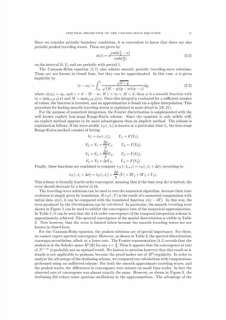
8/3/2019 Xavier Raynaud- On a Shallow Water Wave Equation
http://slidepdf.com/reader/full/xavier-raynaud-on-a-shallow-water-wave-equation 73/161
SPECTRAL PROJECTION OF THE CAMASSA-HOLM EQUATION 11
Since we consider periodic boundary conditions, it is convenient to know that there are alsoperiodic peaked traveling waves. These are given by
φ(x) = d
cosh( 12
−x)
cosh( 12 ) (5.2)
on the interval [0, 1], and are periodic with period 1.The Camassa-Holm equation (1.1) also admits smooth periodic traveling-wave solutions.
These are not known in closed form, but they can be approximated. In this case, φ is givenimplicitly by
|x − x0| =
φφ0
√d − y
(M − y)(y − m)(y − z)dy, (5.3)
where φ(x0) = φ0, and z = d − M − m. If z < m < M < d, then φ is a smooth function withm = minx∈R ϕ(x) and M = maxx∈R ϕ(x). Once this integral is evaluated for a sufficient numberof values, the function is inverted, and an approximation is found via a spline interpolation. Thisprocedure for finding smooth traveling waves is explained in more detail in [18, 21].
For the purpose of numerical integration, the Fourier discretization is supplemented with thewell known explicit four-stage Runge-Kutta scheme. Since the equation is only mildly stiff,an explicit method appears to be more advantageous than an implicit method. The scheme isexplained as follows. If the wave profile vN (·, ti) is known at a particular time ti, the four-stageRunge-Kutta method consists of letting
V 1 = vN (·, ti), Γ1 = F (V 1),
V 2 = V 1 +∆t
2Γ1, Γ2 = F (V 2),
V 3 = V 2 +∆t
2Γ2, Γ3 = F (V 3),
V 4 = V 3 + ∆tΓ3, Γ4 = F (V 4).
Finally, these functions are combined to compute vN (·, ti+1) = vN (·, ti + ∆t), according to
vN (·, ti + ∆t) = vN (·, ti) +∆t
6(Γ1 + 2Γ2 + 2Γ3 + Γ4) .
This scheme is formally fourth-order convergent, meaning that if the time step ∆ t is halved, theerror should decrease by a factor of 16.
The traveling-wave solutions can be used to test the numerical algorithm, because their timeevolution is simply given by translation. If vN (·, T ) is the result of a numerical computation withinitial data φ(x), it can be compared with the translated function φ(x − dT ). In this way, theerror produced by the discretization can be calculated. In particular, the smooth traveling waveshown in Figure 1 can be used to exhibit the convergence rate of the numerical approximation.In Table 1, it can be seen that the 4-th order convergence of the temporal integration scheme isapproximately achieved. The spectral convergence of the spatial discretization is visible in Table
2. Note however, that the error is limited below because the smooth traveling waves are notknown in closed form.For the Camassa-Holm equation, the peakon solutions are of special importance. For these,
we cannot expect spectral convergence. However, as shown in Table 3, the spectral discretizationconverges nevertheless, albeit at a lower rate. The Fourier representation (4.1) reveals that thepeakon is in the Sobolev space H s(R) for any s < 3
2 . Thus it appears that the convergence at rate
of N 1−m is probably not an optimal result. We hasten to mention however that this result as itstands is not applicable to peakons, because the proof makes use of H 4-regularity. In order toanalyze the advantage of the dealiasing scheme, we compared our calculations with computationsperformed using an unfiltered scheme. For both the smooth approximate traveling waves, andthe peaked waves, the differences in convergence were minute on small time scales. In fact theobserved rate of convergence was almost exactly the same. However, as shown in Figure 3, thedealiasing did reduce some spurious oscillations in the approximations. The advantage of the
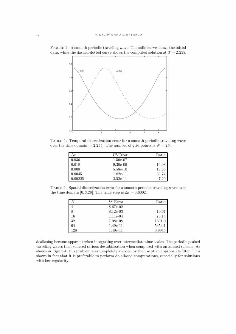
8/3/2019 Xavier Raynaud- On a Shallow Water Wave Equation
http://slidepdf.com/reader/full/xavier-raynaud-on-a-shallow-water-wave-equation 74/161
12 H. KALISCH AND X. RAYNAUD
Figure 1. A smooth periodic traveling wave. The solid curve shows the initialdata, while the dashed-dotted curve shows the computed solution at T = 2.255.
0 1 2 3 4 5 60.2
0.3
0.4
0.5
0.6
0.7
T=0 T=2.255
Table 1. Temporal discretization error for a smooth periodic traveling waveover the time domain [0, 2.255]. The number of grid points is N = 256.
∆t L2-Error Ratio0.036 1.50e-070.018 9.30e-09 16.080.009 5.58e-10 16.66
0.0045 1.82e-11 30.740.00225 2.52e-11 7.20
Table 2. Spatial discretization error for a smooth periodic traveling wave overthe time domain [0, 3.28]. The time step is ∆t = 0.0002.
N L2-Error Ratio4 8.67e-028 8.12e-03 10.6716 1.11e-04 73.1432 7.98e-08 1391.064 1.49e-11 5354.1128 1.49e-11 0.9945
dealiasing became apparent when integrating over intermediate time scales. The periodic peakedtraveling waves then suffered serious destabilization when computed with an aliased scheme. Asshown in Figure 4, this problem was completely avoided by the use of an appropriate filter. Thisshows in fact that it is preferable to perform de-aliased computations, especially for solutionswith low regularity.
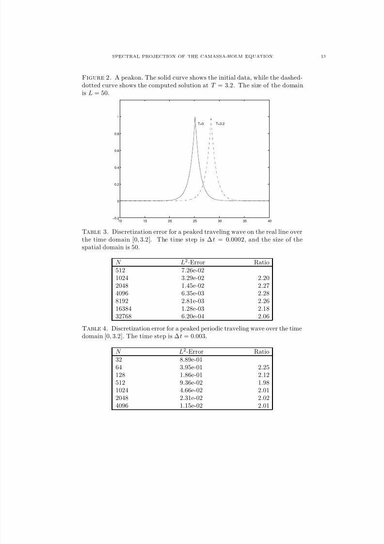
8/3/2019 Xavier Raynaud- On a Shallow Water Wave Equation
http://slidepdf.com/reader/full/xavier-raynaud-on-a-shallow-water-wave-equation 75/161
SPECTRAL PROJECTION OF THE CAMASSA-HOLM EQUATION 13
Figure 2. A peakon. The solid curve shows the initial data, while the dashed-dotted curve shows the computed solution at T = 3.2. The size of the domain
is L = 50.
10 15 20 25 30 35 40−0.2
0
0.2
0.4
0.6
0.8
1
T=0 T=3.2
Table 3. Discretization error for a peaked traveling wave on the real line overthe time domain [0, 3.2]. The time step is ∆t = 0.0002, and the size of thespatial domain is 50.
N L2-Error Ratio512 7.26e-021024 3.29e-02 2.20
2048 1.45e-02 2.274096 6.35e-03 2.288192 2.81e-03 2.2616384 1.28e-03 2.1832768 6.20e-04 2.06
Table 4. Discretization error for a peaked periodic traveling wave over the timedomain [0, 3.2]. The time step is ∆t = 0.003.
N L2-Error Ratio32 8.89e-0164 3.95e-01 2.25128 1.86e-01 2.12
512 9.36e-02 1.981024 4.66e-02 2.012048 2.31e-02 2.024096 1.15e-02 2.01
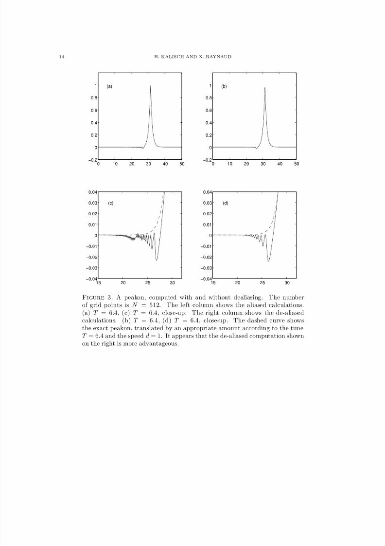
8/3/2019 Xavier Raynaud- On a Shallow Water Wave Equation
http://slidepdf.com/reader/full/xavier-raynaud-on-a-shallow-water-wave-equation 76/161
14 H. KALISCH AND X. RAYNAUD
0 10 20 30 40 50−0.2
0
0.2
0.4
0.6
0.8
1 (a)
0 10 20 30 40 50−0.2
0
0.2
0.4
0.6
0.8
1 (b)
15 20 25 30−0.04
−0.03
−0.02
−0.01
0
0.01
0.02
0.03
0.04
(c)
15 20 25 30−0.04
−0.03
−0.02
−0.01
0
0.01
0.02
0.03
0.04
(d)
Figure 3. A peakon, computed with and without dealiasing. The numberof grid points is N = 512. The left column shows the aliased calculations.(a) T = 6.4, (c) T = 6.4, close-up. The right column shows the de-aliasedcalculations. (b) T = 6.4, (d) T = 6.4, close-up. The dashed curve showsthe exact peakon, translated by an appropriate amount according to the timeT = 6.4 and the speed d = 1. It appears that the de-aliased computation shownon the right is more advantageous.
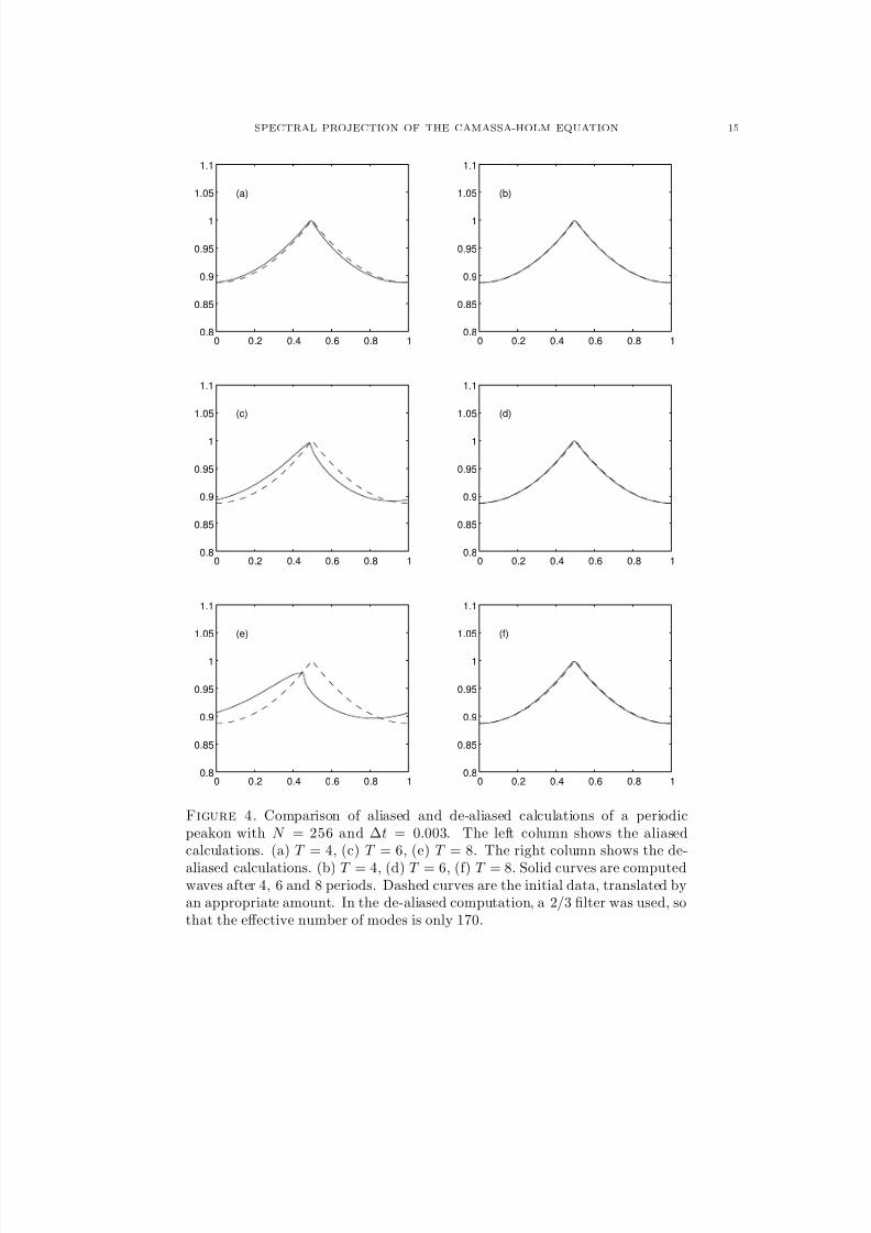
8/3/2019 Xavier Raynaud- On a Shallow Water Wave Equation
http://slidepdf.com/reader/full/xavier-raynaud-on-a-shallow-water-wave-equation 77/161
SPECTRAL PROJECTION OF THE CAMASSA-HOLM EQUATION 15
0 0.2 0.4 0.6 0.8 10.8
0.85
0.9
0.95
1
1.05
1.1
(a)
0 0.2 0.4 0.6 0.8 10.8
0.85
0.9
0.95
1
1.05
1.1
(b)
0 0.2 0.4 0.6 0.8 10.8
0.85
0.9
0.95
1
1.05
1.1
(c)
0 0.2 0.4 0.6 0.8 10.8
0.85
0.9
0.95
1
1.05
1.1
(d)
0 0.2 0.4 0.6 0.8 10.8
0.85
0.9
0.95
1
1.05
1.1
(e)
0 0.2 0.4 0.6 0.8 10.8
0.85
0.9
0.95
1
1.05
1.1
(f)
Figure 4. Comparison of aliased and de-aliased calculations of a periodicpeakon with N = 256 and ∆t = 0.003. The left column shows the aliasedcalculations. (a) T = 4, (c) T = 6, (e) T = 8. The right column shows the de-
aliased calculations. (b) T = 4, (d) T = 6, (f) T = 8. Solid curves are computedwaves after 4, 6 and 8 periods. Dashed curves are the initial data, translated byan appropriate amount. In the de-aliased computation, a 2/3 filter was used, sothat the effective number of modes is only 170.
8/3/2019 Xavier Raynaud- On a Shallow Water Wave Equation
http://slidepdf.com/reader/full/xavier-raynaud-on-a-shallow-water-wave-equation 78/161
16 H. KALISCH AND X. RAYNAUD
References
[1] R. Artebrant and H.J. Schroll, Numerical simulation of Camassa-Holm peakons by adaptive upwinding, toappear in Appl. Num. Math.
[2] R. Camassa, and D. Holm, An integrable shallow water equation with peaked solitons, Phys. Rev. Lett. 71(1993), 1661-1664.
[3] R. Camassa, D. Holm and J. Hyman, A new integrable shallow water equation, Adv. Appl. Mech. 31 (1994),1-33.
[4] A. Constantin, On the scattering problem for the Camassa-Holm equation, Proc. Roy. Soc. London A 457(2001), 953-970.
[5] A. Constantin and J. Escher, Well-posedness, global existence, and blowup phenomena for a perio dic quasi-linear hyperbolic equation, Comm. Pure Appl. Math. 5 (1998), 475-504.
[6] A. Constantin and B. Kolev, On the geometric approach to the motion of inertial mechanical systems, J.Phys. A 35 (2002), R51-R79.
[7] C. Canuto, M.Y. Hussaini, A. Quarteroni and T.A. Zang, Spectral Methods in Fluid Dynamics, Springer,1988.
[8] H.-H. Dai and Y. Huo, Solitary shock waves and other travelling waves in a general compressible hyperelasticrod, Proc. Roy. Soc. London A 456 (2000), 331-363.
[9] A. S. Fokas, On a class of physically important integrable equations, Physica D 87 (1995), 145-150.
[10] B. Fuchssteiner and A. S. Fokas, Symplectic structures, their Bachlund transformation and hereditary sym-metries, Physica D 4 (1981), 47-66.
[11] B. Fuchssteiner, Some tricks from the symmetry-toolbox for nonlinear equations: generalizations of theCamassa-Holm equation, Physica D 95 (1996), 229-243.
[12] C. Gasquet and P. Witomski, Fourier Analysis and Applications, Springer, 1999[13] D.D. Holm, J. Marsden and T. Ratiu, The Euler-Poincare equations and semidirect products with applications
to continuum theories, Adv. Math. 137 (1998), 1-81.[14] H. Holden and X. Raynaud, Convergence of a finite difference scheme for the Camassa-Holm equation, SIAM
J. Numer. Anal. 2006, to appear. paper I in this thesis.[15] H. Holden and X. Raynaud, A convergent numerical scheme for the Camassa–Holm equation based on
multipeakons, Disc. Cont. Dyn. Sys. 14 (2006) 505-523. paper II in this thesis.[16] R. Johnson, Camassa-Holm, Korteweg-de Vries and related models for water waves, J. Fluid Mech. 455
(2002), 63-82.[17] H. Kalisch, Stability of solitary waves for a nonlinearly dispersive equation, Disc. Cont. Dyn. Sys. 10 (2004),
709-716.
[18] H. Kalisch and J. Lenells, Numerical study of traveling-wave solutions for the Camassa-Holm equation,Chaos, Solitons & Fractals 25 (2005) 287-298.
[19] H.-O. Kreiss and J. Oliger, Stability of the Fourier method, SIAM J. Numer. Anal. 16 (1979), 421-433.[20] M. Kunze and G. Schneider, Estimates for the KdV-limit of the Camassa-Holm equation, Lett. Math. Phys.
72 (2005), 17-26.[21] J. Lenells, Traveling wave solutions of the Camassa-Holm equation, J. Diff. Eq. 217 (2005), 393-430.[22] Y. Maday and A. Quarteroni, Error analysis for spectral approximation of the Korteweg-de Vries equation,
RAIRO Modl. Math. Anal. Numr. 22 (1988), 499-529.[23] G. Misiolek, A shallow water equation as a geodesic flow on the Bott-Viroasoro group, J. Geom. Phys. 24
(1998), 203-208.[24] J.E. Pasciak, Spectral and pseudospectral methods for advection equations, Math. Comput. 35 (1980), 1081-
1092.[25] R.L. Seliger, A note on breaking waves, Proc. Roy. Soc. A 303 (1968), 493-496.[26] G.B. Whitham, Linear and Nonlinear Waves, Wiley, 1974.

8/3/2019 Xavier Raynaud- On a Shallow Water Wave Equation
http://slidepdf.com/reader/full/xavier-raynaud-on-a-shallow-water-wave-equation 79/161
8/3/2019 Xavier Raynaud- On a Shallow Water Wave Equation
http://slidepdf.com/reader/full/xavier-raynaud-on-a-shallow-water-wave-equation 80/161
Paper IV
Global conservative solutions of theCamassa–Holm equation – A Lagrangian point of view.
H. Holden and X. RaynaudSubmitted for publication.

8/3/2019 Xavier Raynaud- On a Shallow Water Wave Equation
http://slidepdf.com/reader/full/xavier-raynaud-on-a-shallow-water-wave-equation 81/161
8/3/2019 Xavier Raynaud- On a Shallow Water Wave Equation
http://slidepdf.com/reader/full/xavier-raynaud-on-a-shallow-water-wave-equation 82/161
GLOBAL CONSERVATIVE SOLUTIONSOF THE CAMASSA–HOLM EQUATION – A LAGRANGIAN POINT OF
VIEW
HELGE HOLDEN AND XAVIER RAYNAUD
Abstract. We show that the Camassa–Holm equation ut−uxxt+3uux−2uxuxx−uuxxx = 0possesses a global continuous semigroup of weak conservative solutions for initial data u|t=0in H 1. The result is obtained by introducing a coordinate transformation into Lagrangiancoordinates. To characterize conservative solutions it is necessary to include the energy densitygiven by the positive Radon measure µ with µac = (u2 +u2
x)dx. The total energy is preserved
by the solution.
1. Introduction
The Cauchy problem for the Camassa–Holm equation [7, 8]
ut − uxxt + 2κux + 3uux − 2uxuxx − uuxxx = 0, u|t=0 = u, (1.1)
has received considerable attention the last decade. With κ positive it models, see [25], propaga-tion of unidirectional gravitational waves in a shallow water approximation, with u representingthe fluid velocity. The Camassa–Holm equation has a bi-Hamiltonian structure and is completelyintegrable. It has infinitely many conserved quantities. In particular, for smooth solutions thequantities
udx,
(u2 + u2
x) dx,
(u3 + uu2
x) dx (1.2)
are all time independent.In this article we consider the case κ = 0 on the real line, that is,
ut − uxxt + 3uux − 2uxuxx − uuxxx = 0, (1.3)
and henceforth we refer to (1.3) as the Camassa–Holm equation. The equation can be rewrittenas the following system
ut + uux + P x = 0, (1.4a)
P − P xx = u2 +1
2u2x. (1.4b)
A highly interesting property of the equation is that for a wide class of initial data thesolution experiences wave breaking in finite time in the sense that the solution u remains boundedpointwise while the spatial derivative ux becomes unbounded pointwise. However, the H 1 normof u remains finite. More precisely, Constantin, Escher, and Molinet [12, 14] showed the followingresult: If the initial data u|t=0 = u ∈ H 1(R) and m := u − u is a positive Radon measure, thenequation (1.3) has a unique global weak solution u ∈ C ([0, T ], H 1(R)), for any T positive, withinitial data u. However, any solution with odd initial data u in H 3(R) such that ux(0) < 0 blowsup in a finite time.
2000 Mathematics Subject Classification. Primary: 65M06, 65M12; Secondary: 35B10, 35Q53.Key words and phrases. Camassa–Holm equation, conservative solutions.Supported in part by the Research Council of Norway.
1
8/3/2019 Xavier Raynaud- On a Shallow Water Wave Equation
http://slidepdf.com/reader/full/xavier-raynaud-on-a-shallow-water-wave-equation 83/161
2 H. HOLDEN AND X. RAYNAUD
The problem how to extend the solution beyond wave breaking can nicely be illustrated bystudying an explicit class of solutions. The Camassa–Holm equation possesses solutions, denoted(multi)peakons, of the form
u(t, x) =n
i=1
pi(t)e−|x−qi(t)|, (1.5)
where the ( pi(t), qi(t)) satisfy the explicit system of ordinary differential equations
qi =n
j=1
pje−|qi−qj|, ˙ pi =n
j=1
pi pj sgn(qi − qj)e−|qi−qj |.
Observe that the solution (1.5) is not smooth even with continuous functions ( pi(t), qi(t)); onepossible way to interpret (1.5) as a weak solution of (1.3) is to rewrite the equation (1.3) as
ut +1
2u2 + (1 − ∂ 2x)−1(u2 +
1
2u2x)x
= 0.
Peakons interact in a way similar to that of solitons of the Korteweg–de Vries equation, and wavebreaking may appear when at least two of the qi’s coincide. If all the pi(0) have the same sign, thepeakons move in the same direction. Furthermore, in that case the solution experiences no wavebreaking, and one has a global solution. Higher peakons move faster than the smaller ones, andwhen a higher peakon overtakes a smaller, there is an exchange of mass, but no wave breakingtakes place. Furthermore, the qi(t) remain distinct. However, if some of pi(0) have opposite sign,wave breaking may incur, see, e.g., [3, 26]. For simplicity, consider the case with n = 2 and onepeakon p1(0) > 0 (moving to the right) and one antipeakon p2(0) < 0 (moving to the left). In thesymmetric case ( p1(0) = − p2(0) and q1(0) = −q2(0) < 0) the solution will vanish pointwise atthe collision time t∗ when q1(t∗) = q2(t∗), that is, u(t∗, x) = 0 for all x ∈ R. Clearly, at least twoscenarios are possible; one is to let u(t, x) vanish identically for t > t∗, and the other possibilityis to let the peakon and antipeakon “pass through” each other in a way that is consistent withthe Camassa–Holm equation. In the first case the energy (u2 + u2
x) dx decreases to zero at t∗,
while in the second case, the energy remains constant except at t∗. Clearly, the well-posednessof the equation is a delicate matter in this case. The first solution could be denoted a dissipativesolution, while the second one could be called conservative. Other solutions are also possible.Global dissipative solutions of a more general class of equations were recently derived by Coclite,Holden, and Karlsen [9, 10]. In their approach the solution was obtained by first regularizingthe equation by adding a small diffusion term uxx to the equation, and subsequently analyzingthe vanishing viscosity limit → 0. Multipeakons are fundamental building blocks for generalsolutions. Indeed, if the initial data u is in H 1 and m := u − u is a positive Radon measure,then it can proved, see [23], that one can construct a sequence of multipeakons that convergesin L∞
loc(R; H 1loc(R)) to the unique global solution of the Camassa–Holm equation.The problem of continuation beyond wave breaking was recently considered by Bressan and
Constantin [4]. They reformulated the Camassa–Holm equation as a semilinear system of or-
dinary differential equations taking values in a Banach space. This formulation allowed themto continue the solution beyond collision time, giving a global conservative solution where theenergy is conserved for almost all times. Thus in the context of peakon-antipeakon collisionsthey considered the solution where the peakons and antipeakons “passed through” each other.Local existence of the semilinear system is obtained by a contraction argument. Furthermore,the clever reformulation allows for a global solution where all singularities disappear. Goingback to the original function u, one obtains a global solution of the Camassa–Holm equation.The well-posedness, i.e., the uniqueness and stability of the solution, is resolved as follows. Inaddition to the solution u, one includes a family of non-negative Radon measures µt with densityu2x dx with respect to the Lebesgue measure. The pair (u, µt) constitutes a continuous semigroup,
in particular, one has uniqueness and stability.Very recently, Bressan and Fonte [5, 20] presented another approach to the Camassa–Holm
equation. The flow map u
→u(t) is, as we have seen, neither a continuous map on H 1 nor on
8/3/2019 Xavier Raynaud- On a Shallow Water Wave Equation
http://slidepdf.com/reader/full/xavier-raynaud-on-a-shallow-water-wave-equation 84/161
GLOBAL CONSERVATIVE SOLUTIONS OF THE CAMASSA–HOLM EQUATION 3
L2. However, they introduced a new distance J (u, v) with the property
c1 u − vL1 ≤ J (u, v) ≤ c2 u − vH 1 .
Furthermore, it satisfies
J (u(t), u) ≤ c3 |t| , J (u(t), v(t)) ≤ J (u, v)ec4|t|,
where u(t), v(t) are solutions with initial data u, v, respectively. The distance is introducedby first defining it for multipeakons, using the global, conservative solution described above.Subsequently it is shown that multipeakons are dense in the space H 1. This enables themto construct a semi-group of conservative solutions for the Camassa–Holm equation which iscontinuous with respect to the distance J .
In this paper, as Bressan and Constantin [4], we reformulate the equation using a differentset of variables and obtain a semilinear system of ordinary differential equations. However, thechange of variables we use is distinct from that of Bressan and Constantin and simply correspondsto the transformation between Eulerian and Lagrangian coordinates. Let u = u(t, x) denote the
solution, and y(t, ξ) the corresponding characteristics, thus yt(t, ξ) = u(t, y(t, ξ)). Our newvariables are y(t, ξ),
U (t, ξ) = u(t, y(t, ξ)), H (t, ξ) =
y(t,ξ)
−∞
(u2 + u2x) dx (1.6)
where U corresponds to the Lagrangian velocity while H could be interpreted as the Lagrangiancumulative energy distribution. Furthermore, let
Q(t, ξ) = −1
4
R
sgn(ξ − η)exp− sgn(ξ − η)(y(ξ) − y(η))
U 2yξ + H ξ
(η) dη,
P (t, ξ) =1
4
R
exp− sgn(ξ − η)(y(ξ) − y(η))
U 2yξ + H ξ
dη.
Then one can show that
yt = U,U t = −Q,
H t = U 3 − 2P U,
(1.7)
is equivalent to the Camassa–Holm equation. Global existence of solutions of (1.7) is obtainedstarting from a contraction argument, see Theorem 2.8. The uniqueness issue is resolved byconsidering the set D (see Definition 3.1) which consists of pairs (u, µ) such that (u, µ) ∈ Dif u ∈ H 1(R) and µ is a positive Radon measure whose absolutely continuous part satisfiesµac = (u2 + u2
x) dx. With three Lagrangian variables (y,U,H ) versus two Eulerian variables(u, µ), it is clear that there can be no bijection between the two coordinates systems. However,we define a group of relabeling transformations which acts on the Lagrangian variables and letthe system of equations (1.7) invariant. Using this group, we are able to establish a bijection
between the space of Eulerian variables and the space of Lagrangian variables when we identifyvariables that are invariant under relabeling. This bijection allows us to transform the resultsobtained in the Lagrangian framework (in which the equation is well-posed) into the Eulerianframework (in which the situation is much more subtle). In particular, and this constitutes themain result of this paper, we obtain a metric dD on D and a continuous semi-group of solutionson (D, dD). The distance dD gives D the structure of a complete metric space. This metric iscompared with some more standard topologies, and we obtain that convergence in H 1(R) impliesconvergence in (D, dD) which itself implies convergence in L∞(R), see Propositions 5.1 and 5.2.The properties of the spaces as well as the various mappings between them are described in greatdetail, see Section 3. Our main result, Theorem 4.2, states that for given initial data in D thereexists a unique weak solution of the Camassa–Holm equation. The associated measure µ(t) hasconstant total mass, i.e., µ(t)(R) = µ(0)(R) for all t, which corresponds to the total energy of the system. This is the reason why our solutions are called conservative.
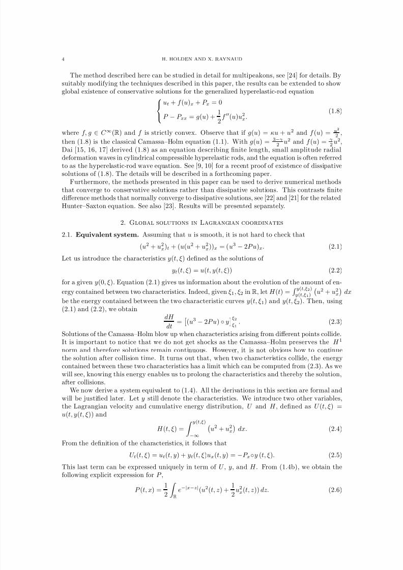
8/3/2019 Xavier Raynaud- On a Shallow Water Wave Equation
http://slidepdf.com/reader/full/xavier-raynaud-on-a-shallow-water-wave-equation 85/161
4 H. HOLDEN AND X. RAYNAUD
The method described here can be studied in detail for multipeakons, see [24] for details. Bysuitably modifying the techniques described in this paper, the results can be extended to showglobal existence of conservative solutions for the generalized hyperelastic-rod equation
ut + f (u)x + P x = 0
P − P xx = g(u) +1
2f (u)u2
x.(1.8)
where f, g ∈ C ∞(R) and f is strictly convex. Observe that if g(u) = κu + u2 and f (u) = u2
2,
then (1.8) is the classical Camassa–Holm equation (1.1). With g(u) = 3−γ2
u2 and f (u) = γ2
u2,Dai [15, 16, 17] derived (1.8) as an equation describing finite length, small amplitude radialdeformation waves in cylindrical compressible hyperelastic rods, and the equation is often referredto as the hyperelastic-rod wave equation. See [9, 10] for a recent proof of existence of dissipativesolutions of (1.8). The details will be described in a forthcoming paper.
Furthermore, the methods presented in this paper can be used to derive numerical methodsthat converge to conservative solutions rather than dissipative solutions. This contrasts finite
difference methods that normally converge to dissipative solutions, see [22] and [21] for the relatedHunter–Saxton equation. See also [23]. Results will be presented separately.
2. Global solutions in Lagrangian coordinates
2.1. Equivalent system. Assuming that u is smooth, it is not hard to check that
(u2 + u2x)t + (u(u2 + u2
x))x = (u3 − 2P u)x. (2.1)
Let us introduce the characteristics y(t, ξ) defined as the solutions of
yt(t, ξ) = u(t, y(t, ξ)) (2.2)
for a given y(0, ξ). Equation (2.1) gives us information about the evolution of the amount of en-
ergy contained between two characteristics. Indeed, given ξ1, ξ2 in R, let H (t) = y(t,ξ2)
y(t,ξ1) u2 + u2x dx
be the energy contained between the two characteristic curves y(t, ξ1) and y(t, ξ2). Then, using(2.1) and (2.2), we obtain
dH
dt=
(u3 − 2P u) ◦ yξ2ξ1
. (2.3)
Solutions of the Camassa–Holm blow up when characteristics arising from different points collide.It is important to notice that we do not get shocks as the Camassa–Holm preserves the H 1
norm and therefore solutions remain continuous. However, it is not obvious how to continuethe solution after collision time. It turns out that, when two characteristics collide, the energycontained between these two characteristics has a limit which can be computed from (2.3). As wewill see, knowing this energy enables us to prolong the characteristics and thereby the solution,after collisions.
We now derive a system equivalent to (1.4). All the derivations in this section are formal and
will be justified later. Let y still denote the characteristics. We introduce two other variables,the Lagrangian velocity and cumulative energy distribution, U and H , defined as U (t, ξ) =u(t, y(t, ξ)) and
H (t, ξ) =
y(t,ξ)
−∞
u2 + u2
x
dx. (2.4)
From the definition of the characteristics, it follows that
U t(t, ξ) = ut(t, y) + yt(t, ξ)ux(t, y) = −P x◦y (t, ξ). (2.5)
This last term can be expressed uniquely in term of U , y, and H . From (1.4b), we obtain thefollowing explicit expression for P ,
P (t, x) =1
2 R e−|x−z|(u2(t, z) +1
2u2x(t, z)) dz. (2.6)
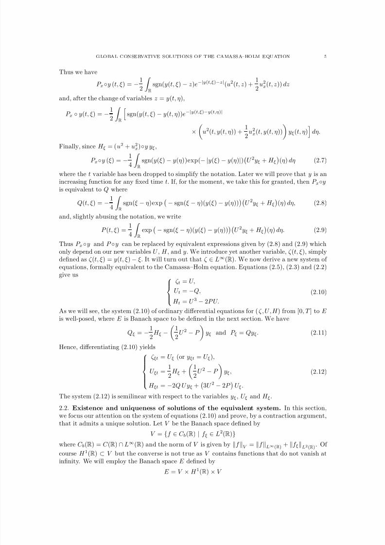
8/3/2019 Xavier Raynaud- On a Shallow Water Wave Equation
http://slidepdf.com/reader/full/xavier-raynaud-on-a-shallow-water-wave-equation 86/161
GLOBAL CONSERVATIVE SOLUTIONS OF THE CAMASSA–HOLM EQUATION 5
Thus we have
P x◦y (t, ξ) = −1
2 R sgn(y(t, ξ) − z)e−|y(t,ξ)−z|(u2(t, z) +1
2u2x(t, z)) dz
and, after the change of variables z = y(t, η),
P x ◦ y(t, ξ) = −1
2
R
sgn(y(t, ξ) − y(t, η))e−|y(t,ξ)−y(t,η)|
×
u2(t, y(t, η)) +1
2u2x(t, y(t, η))
yξ(t, η)
dη.
Finally, since H ξ = (u2 + u2x)◦y yξ,
P x◦y (ξ) = −1
4
R
sgn(y(ξ) − y(η))exp(− |y(ξ) − y(η)|)U 2yξ + H ξ
(η) dη (2.7)
where the t variable has been dropped to simplify the notation. Later we will prove that y is anincreasing function for any fixed time t. If, for the moment, we take this for granted, then P x◦y
is equivalent to Q where
Q(t, ξ) = −1
4
R
sgn(ξ − η)exp− sgn(ξ − η)(y(ξ) − y(η))
U 2yξ + H ξ
(η) dη, (2.8)
and, slightly abusing the notation, we write
P (t, ξ) =1
4
R
exp− sgn(ξ − η)(y(ξ) − y(η))
U 2yξ + H ξ
(η) dη. (2.9)
Thus P x◦y and P ◦y can be replaced by equivalent expressions given by (2.8) and (2.9) whichonly depend on our new variables U , H , and y. We introduce yet another variable, ζ (t, ξ), simplydefined as ζ (t, ξ) = y(t, ξ) − ξ. It will turn out that ζ ∈ L∞(R). We now derive a new system of equations, formally equivalent to the Camassa–Holm equation. Equations (2.5), (2.3) and (2.2)give us
ζ t = U,
U t = −Q,
H t = U 3 − 2P U.
(2.10)
As we will see, the system (2.10) of ordinary differential equations for ( ζ , U , H ) from [0, T ] to E is well-posed, where E is Banach space to be defined in the next section. We have
Qξ = −1
2H ξ −
1
2U 2 − P
yξ and P ξ = Qyξ. (2.11)
Hence, differentiating (2.10) yields
ζ ξt = U ξ (or yξt = U ξ),
U ξt =1
2H ξ +
1
2U 2 − P yξ,
H ξt = −2Q U yξ +
3U 2 − 2P
U ξ.
(2.12)
The system (2.12) is semilinear with respect to the variables yξ, U ξ and H ξ.
2.2. Existence and uniqueness of solutions of the equivalent system. In this section,we focus our attention on the system of equations (2.10) and prove, by a contraction argument,that it admits a unique solution. Let V be the Banach space defined by
V = {f ∈ C b(R) | f ξ ∈ L2(R)}where C b(R) = C (R) ∩ L∞(R) and the norm of V is given by f V = f L∞(R) + f ξL2(R). Of
course H 1(R) ⊂ V but the converse is not true as V contains functions that do not vanish atinfinity. We will employ the Banach space E defined by
E = V
×H 1(R)
×V
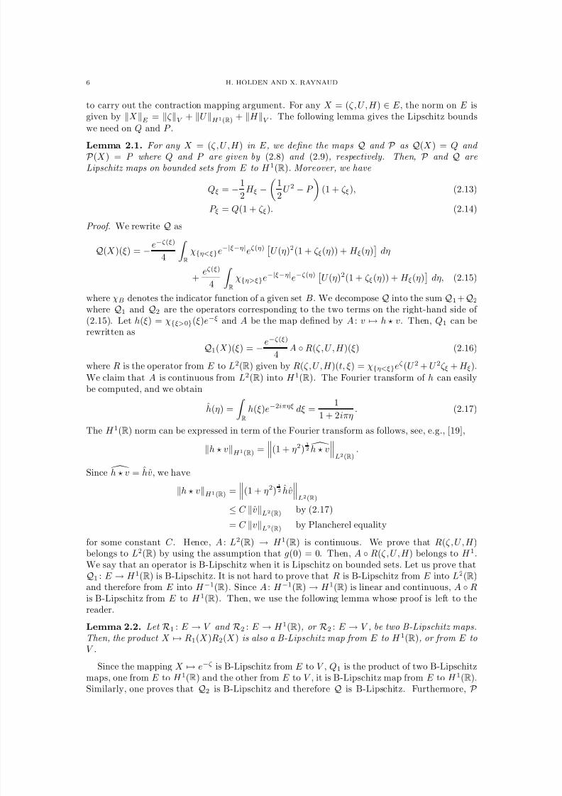
8/3/2019 Xavier Raynaud- On a Shallow Water Wave Equation
http://slidepdf.com/reader/full/xavier-raynaud-on-a-shallow-water-wave-equation 87/161
6 H. HOLDEN AND X. RAYNAUD
to carry out the contraction mapping argument. For any X = (ζ , U , H ) ∈ E , the norm on E isgiven by X E = ζ V + U H 1(R) + H V . The following lemma gives the Lipschitz bounds
we need on Q and P .
Lemma 2.1. For any X = (ζ , U , H ) in E , we define the maps Q and P as Q(X ) = Q and P (X ) = P where Q and P are given by (2.8) and (2.9), respectively. Then, P and Q areLipschitz maps on bounded sets from E to H 1(R). Moreover, we have
Qξ = −1
2H ξ −
1
2U 2 − P
(1 + ζ ξ), (2.13)
P ξ = Q(1 + ζ ξ). (2.14)
Proof. We rewrite Q as
Q(X )(ξ) = −e−ζ(ξ)
4
R
χ{η<ξ}e−|ξ−η|eζ(η)
U (η)2(1 + ζ ξ(η)) + H ξ(η)
dη
+eζ(ξ)
4 R
χ{η>ξ}e−|ξ−η|
e−ζ(η)
U (η)2
(1 + ζ ξ(η)) + H ξ(η)
dη, (2.15)
where χB denotes the indicator function of a given set B. We decompose Q into the sum Q1 +Q2
where Q1 and Q2 are the operators corresponding to the two terms on the right-hand side of (2.15). Let h(ξ) = χ{ξ>0}(ξ)e−ξ and A be the map defined by A : v → h v. Then, Q1 can berewritten as
Q1(X )(ξ) = −e−ζ(ξ)
4A ◦ R(ζ , U , H )(ξ) (2.16)
where R is the operator from E to L2(R) given by R(ζ , U , H )(t, ξ) = χ{η<ξ}eζ(U 2 + U 2ζ ξ + H ξ).
We claim that A is continuous from L2(R) into H 1(R). The Fourier transform of h can easilybe computed, and we obtain
h(η) = R
h(ξ)e−2iπηξ dξ =1
1 + 2iπη
. (2.17)
The H 1(R) norm can be expressed in term of the Fourier transform as follows, see, e.g., [19],
h vH 1(R) =(1 + η2)
12 h vL2(R)
.
Since h v = hv, we have
h vH 1(R) =(1 + η2)
12 hvL2(R)
≤ C vL2(R) by (2.17)
= C vL2(R) by Plancherel equality
for some constant C . Hence, A : L2(R) → H 1(R) is continuous. We prove that R(ζ , U , H )
belongs to L
2
(R
) by using the assumption that g(0) = 0. Then, A ◦ R(ζ , U , H ) belongs to H
1
.We say that an operator is B-Lipschitz when it is Lipschitz on bounded sets. Let us prove thatQ1 : E → H 1(R) is B-Lipschitz. It is not hard to prove that R is B-Lipschitz from E into L2(R)and therefore from E into H −1(R). Since A : H −1(R) → H 1(R) is linear and continuous, A ◦ Ris B-Lipschitz from E to H 1(R). Then, we use the following lemma whose proof is left to thereader.
Lemma 2.2. Let R1 : E → V and R2 : E → H 1(R), or R2 : E → V , be two B-Lipschitz maps.Then, the product X → R1(X )R2(X ) is also a B-Lipschitz map from E to H 1(R), or from E toV .
Since the mapping X → e−ζ is B-Lipschitz from E to V , Q1 is the product of two B-Lipschitzmaps, one from E to H 1(R) and the other from E to V , it is B-Lipschitz map from E to H 1(R).Similarly, one proves that
Q2 is B-Lipschitz and therefore
Qis B-Lipschitz. Furthermore,
P
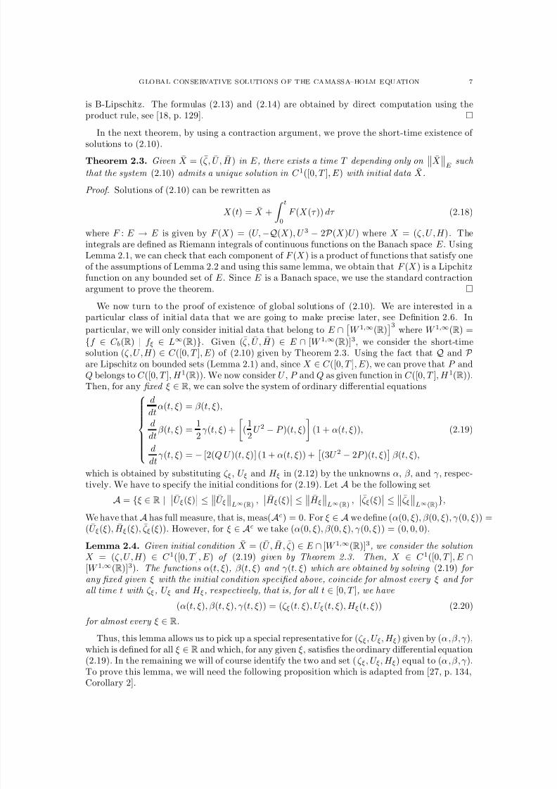
8/3/2019 Xavier Raynaud- On a Shallow Water Wave Equation
http://slidepdf.com/reader/full/xavier-raynaud-on-a-shallow-water-wave-equation 88/161
GLOBAL CONSERVATIVE SOLUTIONS OF THE CAMASSA–HOLM EQUATION 7
is B-Lipschitz. The formulas (2.13) and (2.14) are obtained by direct computation using theproduct rule, see [18, p. 129].
In the next theorem, by using a contraction argument, we prove the short-time existence of solutions to (2.10).
Theorem 2.3. Given X = (ζ , U , H ) in E , there exists a time T depending only on X E
such
that the system (2.10) admits a unique solution in C 1([0, T ], E ) with initial data X .
Proof. Solutions of (2.10) can be rewritten as
X (t) = X +
t0
F (X (τ )) dτ (2.18)
where F : E → E is given by F (X ) = (U, −Q(X ), U 3 − 2P (X )U ) where X = (ζ , U , H ). Theintegrals are defined as Riemann integrals of continuous functions on the Banach space E . UsingLemma 2.1, we can check that each component of F (X ) is a product of functions that satisfy oneof the assumptions of Lemma 2.2 and using this same lemma, we obtain that F (X ) is a Lipchitz
function on any bounded set of E . Since E is a Banach space, we use the standard contractionargument to prove the theorem.
We now turn to the proof of existence of global solutions of (2.10). We are interested in aparticular class of initial data that we are going to make precise later, see Definition 2.6. In
particular, we will only consider initial data that belong to E ∩ W 1,∞(R)3
where W 1,∞(R) =
{f ∈ C b(R) | f ξ ∈ L∞(R)}. Given (ζ , U , H ) ∈ E ∩ [W 1,∞(R)]3, we consider the short-timesolution (ζ , U , H ) ∈ C ([0, T ], E ) of (2.10) given by Theorem 2.3. Using the fact that Q and P are Lipschitz on bounded sets (Lemma 2.1) and, since X ∈ C ([0, T ], E ), we can prove that P andQ belongs to C ([0, T ], H 1(R)). We now consider U , P and Q as given function in C ([0, T ], H 1(R)).Then, for any fixed ξ ∈ R, we can solve the system of ordinary differential equations
d
dt
α(t, ξ) = β (t, ξ),
d
dtβ (t, ξ) =
1
2γ (t, ξ) +
(
1
2U 2 − P )(t, ξ)
(1 + α(t, ξ)),
d
dtγ (t, ξ) = − [2(Q U )(t, ξ)] (1 + α(t, ξ)) +
(3U 2 − 2P )(t, ξ)
β (t, ξ),
(2.19)
which is obtained by substituting ζ ξ , U ξ and H ξ in (2.12) by the unknowns α, β , and γ , respec-tively. We have to specify the initial conditions for (2.19). Let A be the following set
A = {ξ ∈ R | U ξ(ξ) ≤ U ξL∞(R)
,H ξ(ξ) ≤ H ξL∞(R)
,ζ ξ(ξ) ≤ ζ ξL∞(R)
},
We have that A has full measure, that is, meas(Ac) = 0. For ξ ∈ A we define (α(0, ξ), β (0, ξ), γ (0, ξ)) =(U ξ(ξ), H ξ(ξ), ζ ξ(ξ)). However, for ξ ∈ Ac we take (α(0, ξ), β (0, ξ), γ (0, ξ)) = (0, 0, 0).
Lemma 2.4. Given initial condition X = (U , H, ζ )∈
E ∩
[W 1,∞(R)]3, we consider the solution X = (ζ , U , H ) ∈ C 1([0, T ], E ) of (2.19) given by Theorem 2.3. Then, X ∈ C 1([0, T ], E ∩[W 1,∞(R)]3). The functions α(t, ξ), β (t, ξ) and γ (t, ξ) which are obtained by solving (2.19) for any fixed given ξ with the initial condition specified above, coincide for almost every ξ and for all time t with ζ ξ, U ξ and H ξ, respectively, that is, for all t ∈ [0, T ], we have
(α(t, ξ), β (t, ξ), γ (t, ξ)) = (ζ ξ(t, ξ), U ξ(t, ξ), H ξ(t, ξ)) (2.20)
for almost every ξ ∈ R.
Thus, this lemma allows us to pick up a special representative for (ζ ξ, U ξ, H ξ) given by (α,β,γ ),which is defined for all ξ ∈ R and which, for any given ξ, satisfies the ordinary differential equation(2.19). In the remaining we will of course identify the two and set ( ζ ξ, U ξ, H ξ) equal to (α,β,γ ).To prove this lemma, we will need the following proposition which is adapted from [27, p. 134,Corollary 2].
8/3/2019 Xavier Raynaud- On a Shallow Water Wave Equation
http://slidepdf.com/reader/full/xavier-raynaud-on-a-shallow-water-wave-equation 89/161
8 H. HOLDEN AND X. RAYNAUD
Proposition 2.5. Let R be a bounded linear operator on a Banach space X into a Banach space Y . Let f be in C ([0, T ], X ). Then, Rf belongs to C ([0, T ], Y ) and therefore is Riemann integrable, and [0,T ]
Rf (t) dt = R [0,T ]f (t) dt.
Proof of Lemma 2.4. We introduce the Banach space of everywhere bounded function B∞(R)whose norm is naturally given by f B∞(R) = supξ∈R |f (ξ)|. Obviously, C b(R) is included in
B∞(R). We define (α,β,γ ) as the solution of (2.19) in [B∞(R)]3 ∩ L2(R)3
with initial dataas given above. Thus, strictly speaking, this is a different definition than the one given in thelemma but we will see that they are in fact equivalent. We note that the system (2.19) is affine (itconsists of a sum of a linear transformation and a constant) and therefore it is not hard to prove,
by using a contraction argument in [B∞(R)]3 ∩ L2(R)3
, the short-time existence of solutions.Moreover, the solution exists on [0, T ], the interval on which (ζ , U , H ) is defined. Let us assumethe opposite. Then, Z 1(t) = α(t, · )B∞(R)∩L2(R) + β (t, · )B∞(R)∩L2(R) + γ (t, · )B∞(R)∩L2(R)
has to blow up when t approaches some time strictly smaller than T . We rewrite (2.19) in integralform:
α(t) = α(0) + t
0
β (τ ) dτ,
β (t) = β (0) +
t0
1
2γ + (
1
2U 2 − P )(1 + α)
(τ ) dτ,
γ (t) = γ (0) +
t0
−2Q U (1 + α) + (3U 2 − 2P )β
(τ ) dτ.
(2.21)
Note that in (2.21) all the terms belong to B∞(R) ∩ L2(R) and the equalities hold in this space.After taking the norms on both sides of the three equations in (2.21) and adding them term byterm, we obtain the following inequality
Z 1(t) ≤ Z 1(0) + CT + C t
0
Z 1(τ ) dτ
where C is a constant which depends on the C ([0, T ], H 1(R))-norms of U , P and Q, which,by assumption, are bounded. From Gronwall’s lemma, we get Z 1(t) ≤ (Z 1(0) + CT )eCT andtherefore Z 1(t) cannot blow up and α, β and γ belong to C 1([0, T ], B∞(R) ∩ L2(R)). For anygiven ξ, the map f → f (ξ) from B∞(R) to R is linear and continuous. Hence, after applying thismap to each term in (2.21) and using Proposition 2.5, we recover the original definition of α, β and γ as solutions, for any given ξ ∈ R, of the system (2.19) of ordinary differential equationsin R3. The derivation map ∂ ξ is continuous from V and H 1(R) into L2(R). We can apply it toeach term in (2.10) written in integral from and, by Proposition 2.5, this map commutes withthe integral. We end up with, after using (2.13) and (2.14),
ζ ξ(t) = ζ ξ + t
0
U ξ(τ ) dτ,
U ξ(t) = U ξ +
t
0
1
2H ξ + (
1
2U 2 − P )(1 + ζ ξ)
(τ ) dτ,
H ξ(t) = H ξ +
t0
−2Q U (1 + ζ ξ) + (3U 2 − 2P )U ξ
(τ ) dτ.
(2.22)
The injection map from B∞(R) ∩ L2(R) to L2(R) is of course continuous, we can apply it to(2.21) and again use Proposition 2.5. Then, we can subtract each equation in (2.22) fromthe corresponding one in (2.21), take the norm and add them. After introducing Z 2(t) =α(t, · ) − ζ ξ(t, · )L2(R) + β (t, · ) − U ξ(t, · )L2(R) + γ (t, · ) − H ξ(t, · )L2(R), we end up with
the following equation
Z 2(t) ≤ Z 2(0) + C t
0
Z 2(τ ) dτ
8/3/2019 Xavier Raynaud- On a Shallow Water Wave Equation
http://slidepdf.com/reader/full/xavier-raynaud-on-a-shallow-water-wave-equation 90/161
GLOBAL CONSERVATIVE SOLUTIONS OF THE CAMASSA–HOLM EQUATION 9
where C is a constant which, again, only depends on the C ([0, T ], H 1(R))-norms, of U , P andQ. By assumption on the initial conditions, we have Z 2(0) = 0 because α(0) = ζ ξ , β (0) = U ξ,γ (0) = H ξ almost everywhere and therefore, by Gronwall’s lemma, we get Z 2(t) = 0 for all
t ∈ [0, T ]. This is just a reformulation of (2.20), and this concludes the proof of the lemma.
It is possible to carry out the contraction argument of Theorem 2.3 in the Banach space[W 1,∞(R)]3 but the topology on [W 1,∞(R)]3 turns out to be too strong for our purpose andthat is why we prefer E whose topology is in some sense weaker. Our goal is to find solutionsof (1.4) with initial data u in H 1 because H 1 is the natural space for the equation. Theorem2.3 gives us the existence of solutions to (2.10) for initial data in E . Therefore we have to findinitial conditions that match the initial data u and belong to E . A natural choice would be touse y(ξ) = y(0, ξ) = ξ and U (ξ) = u(ξ). Then y(t, ξ) gives the position of the particle which isat ξ at time t = 0. But, if we make this choice, then H ξ = u2 + u2
x and H ξ does not belong toL2(R) in general. We consider instead (y, U , H ) given by the relations
ξ = y(ξ)
−∞ (u
2
+ u
2
x) dx + y(ξ),¯U = u◦y , and
¯H = y−∞
u
2
+ u
2
x
dx. (2.23)
Later (see Remark 3.10), we will prove that (y − Id, U , H ) belongs to G where G is defined asfollows.
Definition 2.6. The set G is composed of all (ζ , U , H ) ∈ E such that
(ζ , U , H ) ∈ W 1,∞(R)3
, (2.24a)
yξ ≥ 0, H ξ ≥ 0, yξ + H ξ > 0 almost everywhere, and limξ→−∞
H (ξ) = 0, (2.24b)
yξH ξ = y2ξU 2 + U 2ξ almost everywhere, (2.24c)
where we denote y(ξ) = ζ (ξ) + ξ.
Note that if all functions are smooth and yξ > 0, we have ux ◦ y = U ξyξ and condition (2.24c)is equivalent to (2.4). For initial data in G, the solution of (2.10) exists globally.
Lemma 2.7. Given initial data X = (ζ , U , H ) in G, let X (t) = (ζ (t), U (t), H (t)) be the short-time solution of (2.10) in C ([0, T ], E ) for some T > 0 with initial data (ζ, U , H ). Then,
(i) X (t) belongs to G for all t ∈ [0, T ],(ii) for almost every t ∈ [0, T ], yξ(t, ξ) > 0 for almost every ξ ∈ R,(iii) For all t ∈ [0, T ], limξ→±∞ H (t, ξ) exists and is independent of time.
We denote by A the set where the absolute values of ζ ξ(ξ), H ξ(ξ), and U ξ(ξ) all are smallerthanX
[W 1,∞(R)]3and where the inequalities in (2.24b) and (2.24c) are satisfied for yξ, U ξ and
H ξ. By assumption, we have meas(Ac) = 0 and we set (U ξ, H ξ, ζ ξ) equal to zero on Ac. Thus,as allowed by Lemma 2.4, we choose a special representative for ( ζ (t, ξ), U (t, ξ), H (t, ξ)) whichsatisfies (2.12) as an ordinary differential equation, for every ξ ∈ R.
Proof. (i ) We already proved in Lemma 2.4 that the space [W 1,∞(R)]3 is preserved and thereforeX (t) satisfies (2.24a) for all t ∈ [0, T ]. Let us prove that (2.24c) and the inequalities in (2.24b)hold for any ξ ∈ A and therefore almost everywhere. We consider a fixed ξ in A and drop it inthe notations when there is no ambiguity. From (2.12), we have, on the one hand,
(yξH ξ)t = yξtH ξ + H ξtyξ = U ξH ξ + (3U 2U ξ − 2yξQU − 2P U ξ)yξ,
and, on the other hand,
(y2ξU 2 + U 2ξ )t = 2yξtyξU 2 + 2y2
ξU tU + 2U ξtU ξ
= 3U ξU 2yξ − 2P U ξyξ + H ξU ξ − 2y2ξQU.
8/3/2019 Xavier Raynaud- On a Shallow Water Wave Equation
http://slidepdf.com/reader/full/xavier-raynaud-on-a-shallow-water-wave-equation 91/161
10 H. HOLDEN AND X. RAYNAUD
Thus, (yξH ξ − y2ξU 2 − U 2ξ )t = 0, and since yξH ξ(0) = (y2
ξU 2 + U 2ξ )(0), we have yξH ξ(t) =
(y2ξU 2 + U 2ξ )(t) for all t ∈ [0, T ]. We have proved (2.24c). Let us introduce t∗ given by
t∗
= sup{t ∈ [0, T ] | yξ(t
) ≥ 0 for all t
∈ [0, t]}.Here we recall that we consider a fixed ξ ∈ A and dropped it in the notation. Assume thatt∗ < T . Since yξ(t) is continuous with respect to time, we have
yξ(t∗) = 0. (2.25)
Hence, from (2.24c) that we just proved, U ξ(t∗) = 0 and, by (2.12),
yξt(t∗) = U ξ(t∗) = 0. (2.26)
From (2.12), since yξ(t∗) = U ξ(t∗) = 0, we get
yξtt(t∗) = U ξt(t∗) =1
2H ξ(t∗). (2.27)
If H ξ
(t∗) = 0, then (yξ
, U ξ
, H ξ
)(t∗) = (0, 0, 0) and, by the uniqueness of the solution of (2.12),seen as a system of ordinary differential equations, we must have ( yξ, U ξ, H ξ)(t) = 0 for allt ∈ [0, T ]. This contradicts the fact that yξ(0) and H ξ(0) cannot vanish at the same time(yξ + H ξ > 0 for all ξ ∈ A). If H ξ(t∗) < 0, then yξtt(t∗) < 0 and, because of (2.25) and (2.26),there exists a neighborhood U of t∗ such that y(t) < 0 for all t ∈ U \ {t∗}. This contradicts thedefinition of t∗. Hence, H ξ(t∗) > 0 and, since we now have yξ(t∗) = yξt(t∗) = 0 and yξtt(t∗) > 0,there exists a neighborhood of t∗ that we again denote U such that yξ(t) > 0 for all t ∈ U \ {t∗}.This contradicts the fact that t∗ < T , and we have proved the first inequality in (2.24b), namelythat yξ(t) ≥ 0 for all t ∈ [0, T ]. Let us prove that H ξ(t) ≥ 0 for all t ∈ [0, T ]. This follows from(2.24c) when yξ(t) > 0. Now, if yξ(t) = 0, then U ξ(t) = 0 from (2.24c) and we have seen thatH ξ(t) < 0 would imply that yξ(t) < 0 for some t in a punctured neighborhood of t, which isimpossible. Hence, H ξ(t) ≥ 0 and we have proved the second inequality in (2.24b). Assume thatthe third inequality in (2.24c) does not hold. Then, by continuity, there exists a time t
∈[0, T ]
such that (yξ + H ξ)(t) = 0. Since yξ and H ξ are positive, we must have yξ(t) = H ξ(t) = 0 and,by (2.24c), U ξ(t) = 0. Since zero is a solution of (2.12), this implies that yξ(0) = U ξ(0) = H ξ(0),which contradicts (yξ + H ξ)(0) > 0. The fact that limξ→−∞ H (t, ξ) = 0 will be proved below in(iii ).
(ii ) We define the set
N = {(t, ξ) ∈ [0, T ] ×R | yξ(t, ξ) = 0}.
Fubini’s theorem gives us
meas( N ) =
R
meas( N ξ) dξ =
[0,T ]
meas( N t) dt (2.28)
where N ξ and N t are the ξ-section and t-section of N , respectively, that is,
N ξ = {t ∈ [0, T ] | yξ(t, ξ) = 0} and N t = {ξ ∈R
| yξ(t, ξ) = 0}.Let us prove that, for all ξ ∈ A, meas( N ξ) = 0. If we consider the sets N nξ defined as
N nξ = {t ∈ [0, T ] | yξ(t, ξ) = 0 and yξ(t, ξ) > 0 for all t ∈ [t − 1/n,t + 1/n] \ {t}},
then
N ξ =n∈N
N nξ . (2.29)
Indeed, for all t ∈ N ξ, we have yξ(t, ξ) = 0, yξt(t, ξ) = 0 from (2.24c) and (2.12) and yξtt(t, ξ) =12
H ξ(t, ξ) > 0 from (2.12) and (2.24b) (yξ and H ξ cannot vanish at the same time for ξ ∈ A).This implies that, on a small punctured neighborhood of t, yξ is strictly positive. Hence, tbelongs to some N nξ for n large enough. This proves (2.29). The set N nξ consists of isolated
points that are countable since, by definition, they are separated by a distance larger than 1/n
8/3/2019 Xavier Raynaud- On a Shallow Water Wave Equation
http://slidepdf.com/reader/full/xavier-raynaud-on-a-shallow-water-wave-equation 92/161
GLOBAL CONSERVATIVE SOLUTIONS OF THE CAMASSA–HOLM EQUATION 11
from one another. This means that meas( N nξ ) = 0 and, by the subadditivity of the measure,
meas( N ξ) = 0. It follows from (2.28) and since meas(Ac) = 0 that
meas( N
t) = 0 for almost every t∈
[0, T ]. (2.30)
We denote by K the set of times such that meas( N t) > 0, i.e.,
K = {t ∈ R+ | meas( N t) > 0} . (2.31)
By (2.30), meas(K) = 0. For all t ∈ Kc, yξ > 0 almost everywhere and, therefore, y(t, ξ) isstrictly increasing and invertible (with respect to ξ).
(iii ) For any given t ∈ [0, T ], since H ξ(t, ξ) ≥ 0, H (t, ξ) is an increasing function with respectto ξ and therefore, as H (t, · ) ∈ L∞(R), H (t, ξ) has a limit when ξ → ±∞. We denote thoselimits H (t, ±∞). Since U (t, · ) ∈ H 1(R), we have limξ→±∞ U (t, ξ) = 0 for all t ∈ [0, T ]. We have
H (t, ξ) = H (0, ξ) +
t0
U 3 − 2P U
(τ, ξ) dτ. (2.32)
We let ξ tend to ±∞. Since U and P are bounded in L∞([0, T ] × R), we can apply the
Lebesgue dominated convergence theorem and it follows from (2.32), as limξ→±∞ U (t, ξ) = 0,that H (t, ±∞) = H (0, ±∞) for all t ∈ [0, T ]. Since X ∈ G, H (0, −∞) = 0 and thereforeH (t, −∞) = 0 for all t ∈ [0, T ].
We are now ready to prove global existence of solutions to (2.10).
Theorem 2.8. For any X = (y, U , H ) ∈ G, the system (2.10) admits a unique global solution X (t) = (y(t), U (t), H (t)) in C 1(R+, E ) with initial data X = (y, U , H ). We have X (t) ∈ G for all times. If we equip G with the topology inducted by the E -norm, then the mapping S : G×R+ → Gdefined as
S t(X ) = X (t)
is a continuous semigroup.
Proof. The solution has a finite time of existence T only if
(ζ , U , H )(t,
·)
E blows up when t
tends to T because, otherwise, by Theorem 2.3, the solution can be prolongated by a small timeinterval beyond T . Let (ζ , U , H ) be a solution of (2.10) in C ([0, T ), E ) with initial data (ζ , U , H ).We want to prove that
supt∈[0,T )
(ζ (t, · ), U (t, · ), H (t, · ))E < ∞. (2.33)
We have already seen that H (t, ξ) is an increasing function in ξ for all t and, from Lemma 2.7, wehave limξ→∞ H (t, ξ) = limξ→∞ H (0, ξ). This shows that supt∈[0,T ) H (t, · )L∞(R) is bounded
byH L∞(R)
and therefore is finite. To simplify the notation we suppress the dependence in t
for the moment. We have
U 2(ξ) = 2
ξ−∞
U (η)U ξ(η) dη = 2
{η≤ξ|yξ(η)>0}
U (η)U ξ(η) dη (2.34)
since, from (2.24c), U ξ(ξ) = 0 when yξ(ξ) = 0. For almost every ξ such that yξ(ξ) > 0, we have
|U (ξ)U ξ(ξ)| =
√yξU (ξ)U ξ(ξ)
yξ(ξ)
≤ 1
2
U (ξ)2yξ(ξ) +
U 2ξ (ξ)
yξ(ξ)
=
1
2H ξ(ξ),
from (2.24c). Inserting this inequality in (2.34), we obtain U 2(ξ) ≤ H (ξ) and supt∈[0,T ) U (t, · )L∞(R)
is therefore finite. Then, from the governing equation (2.10), it follows that
|ζ (t, ξ)| ≤ |ζ (0, ξ)| + supt∈[0,T )
U (t, · )L∞(R) T
and supt∈[0,T ) ζ (t, · )L∞(R) < ∞. Let us prove that supt∈[0,T ) Q(t, · )L∞(R) < ∞. After one
integration by parts, Q can be rewritten as
Q(t, ξ) = −1
4 R e−|y(ξ)−y(η)|yξ(η) sgn(ξ − η)U (η)2 − H (η) dη − 1
2H (t, ξ).
8/3/2019 Xavier Raynaud- On a Shallow Water Wave Equation
http://slidepdf.com/reader/full/xavier-raynaud-on-a-shallow-water-wave-equation 93/161
12 H. HOLDEN AND X. RAYNAUD
Hence, we get, after a change of variable,
|Q(t, ξ)| ≤ C R e−|y(ξ)−y(η)|yξ(η) dη + C ≤ 3C,
where the constant C is a constant which depends only on supt∈[0,T ) H (t, · )L∞(R) and supt∈[0,T ) U (t, · )L∞(R).
Similarly, one proves that that P (t, · )L∞(R) < ∞. We denote
C 1 = supt∈[0,T )
{U (t, · )L∞(R) + H (t, · )L∞(R)
+ ζ (t, · )L∞(R) + P (t, · )L∞(R) + Q(t, · )L∞(R)}.
We have just proved that C 1 < ∞. Let t ∈ [0, T ). Looking back at (2.16) and the definition of R, we obtain that
R(t, · )L2(R) ≤ C (U (t, · )L2(R) + ζ ξ(t, · )L2(R) + H ξ(t, · )L2(R))
for some constant C depending only on C 1. Since A is a continuous linear mapping from L2(R)to H 1(R), we get
A ◦ R(t, · )L2(R) ≤ C (U (t, · )L2(R) + ζ ξ(t, · )L2(R) + H ξ(t, · )L2(R))
for another constant C which again only depends on C 1. From now on, we denote generically byC such constants that only depends on C 1. From (2.16), as
e−ζ(t, · )L∞(R)
≤ C , we obtain that
Q1(t, · )L2(R) ≤ C (U (t, · )L2(R) + ζ ξ(t, · )L2(R) + H ξ(t, · )L2(R))
The same bound holds for Q2 and therefore
Q(t, · )L2(R) ≤ C (U (t, · )L2(R) + ζ ξ(t, · )L2(R) + H ξ(t, · )L2(R)). (2.35)
Similarly, one proves
P (t, · )L2(R) ≤ C (U (t, · )L2(R) + ζ ξ(t, · )L2(R) + H ξ(t, · )L2(R)). (2.36)
Let Z (t) =
U (t,
·)
L2(R) +
ζ ξ(t,
·)
L2(R)
+
U ξ(t,
·)
L2(R)
+
H ξ(t,
·)
L2(R)
, then the theorem
will be proved once we have established that sup t∈[0,T ) Z (t) < ∞. From the integrated versionof (2.10) and (2.22), after taking the L2(R)-norms on both sides, adding the relevant terms andusing (2.36), we obtain
Z (t) ≤ Z (0) + C
t0
Z (τ ) dτ.
Hence, Gronwall’s lemma gives us that supt∈[0,T ) Z (t) < ∞. From standard ordinary differentialequation theory, we infer that S t is a continuous semi-group.
3. From Eulerian to Lagrangian coordinates and vice versa
As noted in [4], even if H 1(R) is a natural space for the equation, there is no hope to obtaina semigroup of solutions by only considering H 1(R). Thus, we introduce the following space D,which characterizes the solutions in Eulerian coordinates:
Definition 3.1. The set D is composed of all pairs (u, µ) such that u belongs to H 1(R) and µis a positive finite Radon measure whose absolute continuous part, µac, satisfies
µac = (u2 + u2x) dx. (3.1)
We derived the equivalent system (2.10) by using characteristics. Since y satisfies (2.2), y, for agiven ξ, can also be seen as the position of a particle evolving in the velocity field u, where u is thesolution of the Camassa–Holm equation. We are then working in Lagrangian coordinates. In [13],the Camassa–Holm equation is derived as a geodesic equation on the group of diffeomorphismequipped with a right-invariant metric. In the present paper, the geodesic curves correspond toy(t, · ). Note that y does not remain a diffeomorphism since it can become non invertible, whichagrees with the fact that the solutions of the geodesic equation may break down, see [11]. Theright-invariance of the metric can be interpreted as an invariance with respect to relabeling as
8/3/2019 Xavier Raynaud- On a Shallow Water Wave Equation
http://slidepdf.com/reader/full/xavier-raynaud-on-a-shallow-water-wave-equation 94/161
GLOBAL CONSERVATIVE SOLUTIONS OF THE CAMASSA–HOLM EQUATION 13
noted in [2]. This is a property that we also observe in our setting. We denote by G the subgroupof the group of homeomorphisms from R to R such that
f −
Id and f −1
−Id both belong to W 1,∞(R) (3.2)
where Id denotes the identity function. The set G can be interpreted as the set of relabelingfunctions. For any α > 1, we introduce the subsets Gα of G defined by
Gα = {f ∈ G | f − IdW 1,∞(R) +f −1 − IdW 1,∞(R)
≤ α}.
The subsets Gα do not possess the group structure of G. The next lemma provides a usefulcharacterization of Gα.
Lemma 3.2. Let α ≥ 0. If f belongs to Gα, then 1/(1 + α) ≤ f ξ ≤ 1 + α almost everywhere.Conversely, if f is absolutely continuous, f − Id ∈ L∞(R) and there exists c ≥ 1 such that 1/c ≤ f ξ ≤ c almost everywhere, then f ∈ Gα for some α depending only on c and f − IdL∞(R).
Proof. Given f
∈Gα, let B be the set of points where f −1 is differentiable. Rademacher’s
theorem says that meas(Bc) = 0. For any ξ ∈ f −1(B), we have
limξ→ξ
f −1(f (ξ)) − f −1(f (ξ))
f (ξ) − f (ξ)= (f −1)ξ(f (ξ))
because f is continuous and f −1 is differentiable at f (ξ). On the other hand, we have
f −1(f (ξ)) − f −1(f (ξ))
f (ξ) − f (ξ)=
ξ − ξ
f (ξ) − f (ξ).
Hence, f is differentiable for any ξ ∈ f −1(B) and
f ξ(ξ) ≥ 1
(f −1)ξL∞(R)
≥ 1
1 + α. (3.3)
The estimate (3.3) holds only on f −1
(B) but, since meas(Bc
) = 0 and f −1
is Lipschitz andone-to-one, meas(f −1(Bc)) = 0 (see, e.g., [1, Remark 2.72]), and therefore (3.3) holds almosteverywhere. We have f ξ ≤ 1 + f ξ − 1L∞(R)
≤ 1 + α.
Let us now consider a function f which is absolutely continuous and such that f −Id ∈ L∞(R)and 1/c ≤ f ξ ≤ c almost everywhere for some c ≥ 1. Since f ξ is bounded, f and therefore f − Idare Lipschitz and f − Id ∈ W 1,∞(R). Since f ξ ≥ 1/c almost everywhere, f is strictly increasingand, since it is also continuous, it is invertible. As f is Lipschitz, we can make the followingchange of variables (see, for example, [1]) and get that, for all ξ1, ξ2 in R such that ξ1 < ξ2,
f −1(ξ2) − f −1(ξ1) =
[f −1(ξ1),f −1(ξ2)]
f ξf ξ
dξ ≤ c(ξ2 − ξ1).
Hence, f −1 is Lipschitz and (f −1)ξ ≤ c. We have f −1(ξ) − ξ = ξ − f (ξ) for ξ = f (ξ) and
therefore f − IdL∞
(R) =
f
−1
− IdL∞
(R). Finally, we getf − IdW 1,∞(R) +f −1 − IdW 1,∞(R)
≤ 2 f − IdW 1,∞(R) + 2
+ f ξL∞(R) +(f −1)ξL∞(R)
≤ 2 f − IdL∞(R) + 2 + 2c.
We define the subsets F α and F of G as follows
F α = {X = (y,U,H ) ∈ G | y + H ∈ Gα},
and
F =
{X = (y,U,H )
∈ G |y + H
∈G
}.
8/3/2019 Xavier Raynaud- On a Shallow Water Wave Equation
http://slidepdf.com/reader/full/xavier-raynaud-on-a-shallow-water-wave-equation 95/161
14 H. HOLDEN AND X. RAYNAUD
For α = 0, G0 = {Id}. As we will see, the space F 0 will play a special role. These sets arerelevant only because they are in some sense preserved by the governing equation (2.10) as thenext lemma shows.
Lemma 3.3. The space F is preserved by the governing equation (2.10). More precisely, given α, T ≥ 0 and X ∈ F α, we have
S t(X ) ∈ F α for all t ∈ [0, T ] where α only depends on T , α and
X E
.
Proof. Let X = (y, U , H ) ∈ F α, we denote X (t) = (y(t), U (t), H (t)) the solution of (2.10) withinitial data X and set h(t, ξ) = y(t, ξ) + H (t, ξ), h(ξ) = y(ξ) + H (ξ). By definition, we haveh ∈ Gα and, from Lemma 3.2, 1/c ≤ hξ ≤ c almost everywhere, for some constant c > 1depending only α. We consider a fixed ξ and drop it in the notation. Applying Gronwall’sinequality backward in time to (2.12), we obtain
|yξ(0)| + |H ξ(0)| + |U ξ(0)| ≤ eCT (|yξ(t)| + |H ξ(t)| + |U ξ(t)|) (3.4)
for some constant C which depends on X (t)C ([0,T ],E), which itself depends only on
X E and
T . From (2.24c), we have
|U ξ(t)| ≤
yξ(t)H ξ(t) ≤ 1
2(yξ(t) + H ξ(t)).
Hence, since yξ and H ξ are positive, (3.4) gives us
1
c≤ yξ + H ξ ≤ 3
2eCT (yξ(t) + H ξ(t)),
and hξ(t) = yξ(t) + H ξ(t) ≥ 23ce−CT . Similarly, by applying Gronwall’s lemma forward in time,
we obtain yξ(t) + H ξ(t) ≤ 32 ceCT . We have (y + H )(t) − ξL∞(R) ≤ X (t)C ([0,T ],E) ≤ C for
another constant C which also only depends on
X E
and T . Hence, applying Lemma 3.2, we
obtain that y(t,
·) + H (t,
·)
∈Gα and therefore X (t)
∈ F α for some α depending only on α,
T and
X E.
For the sake of simplicity, for any X = (y,U,H ) ∈ F and any function f ∈ G, we denote(y ◦ f, U ◦ f, H ◦ f ) by X ◦ f .
Proposition 3.4. The map from G × F to F given by (f, X ) → X ◦ f defines an action of thegroup G on F .Proof. We have to prove that X ◦ f belongs to F for any X = (y,U,H ) ∈ F and f ∈ G. Wedenote X = (y, U , H ) = X ◦f . As compositions of two Lipschitz maps, y, U and H are Lipschitz.We have
y − IdL∞(R) ≤ y ◦ f − f L∞(R) + f − IdL∞(R)
≤ y
−Id
L∞(R) +
f
−Id
L∞(R) < +
∞.
Hence, (y − Id, U , H ) ∈ [W 1,∞(R)]3. Let us prove that
yξ = yξ◦f f ξ, U ξ = U ξ◦f f ξ and H ξ = H ξ◦f f ξ (3.5)
almost everywhere. Let B1 be the set where y is differentiable and B2 the set where y and f are differentiable. Using Radamacher’s theorem, we get that meas(Bc
1) = meas(Bc2) = 0. For
ξ ∈ B3 = B2 ∩ f −1(B1), we consider a sequence ξi converging to ξ (ξi = ξ). We have
y(f (ξi)) − y(f (ξ))
f (ξi) − f (ξ)
f (ξi) − f (ξ)
ξi − ξ=
y(ξi) − y(ξ)
ξi − ξ. (3.6)
Since f is continuous, f (ξi) converges to f (ξ) and, as y is differentiable at f (ξ), the left-handside of (3.6) tends to yξ◦f (ξ) f ξ(ξ). The right-hand side of (3.6) tends to yξ(ξ), and we get that
yξ(f (ξ))f ξ(ξ) = yξ(ξ) (3.7)
8/3/2019 Xavier Raynaud- On a Shallow Water Wave Equation
http://slidepdf.com/reader/full/xavier-raynaud-on-a-shallow-water-wave-equation 96/161
GLOBAL CONSERVATIVE SOLUTIONS OF THE CAMASSA–HOLM EQUATION 15
for all ξ ∈ B3. Since f −1 is Lipschitz, one-to-one and meas(Bc1) = 0, we have meas(f −1(B1)c) = 0
and therefore (3.7) holds everywhere. One proves the two other identities in (3.5) similarly.From Lemma 3.2, we have that f ξ > 0 almost everywhere. Then, using (3.5) we easily check
that (2.24b) and (2.24c) are fulfilled. Thus, we have proved that (y − Id, U , H ) fulfills (2.24). Itremains to prove that (y − Id, U , H ) ∈ E . Since f ∈ G, f ∈ Gα for some large enough α and, byLemma 3.2, there exists a constant c > 0 such that 1/c ≤ f ξ ≤ c almost everywhere. We have,after a change of variables,U 2L2(R)
=
R
(U ◦f )2 dξ ≤ c
R
(U ◦f )2f ξ dξ = c U 2L2(R) .
Hence, U ∈ L2(R). Similarly, one proves that yξ − 1, U ξ and H ξ belong to L2(R) and therefore(y,U,H ) ∈ G. We have y + H = (y + H ) ◦ f which implies, since y + H and f belongs to G andG is a group, that y + H ∈ G. Therefore X ∈ F and the proposition is proved.
Since G is acting on F , we can consider the quotient space F /G of F with respect to theaction of the group G. The equivalence relation on
F is defined as follows: For any X, X
∈ F ,
X and X are equivalent if there exists f ∈ G such that X = X ◦ f . We denote by Π(X ) = [X ]the projection of F into the quotient space F /G. We introduce the mapping Γ : F → F 0 givenby
Γ(X ) = X ◦( y + H )−1
for any X = (y,U,H ) ∈ F . We have Γ(X ) = X when X ∈ F 0. It is not hard to prove Γ isinvariant under the G action, that is, Γ(X ◦ f ) = Γ(X ) for any X ∈ F and f ∈ G. Hence,
there corresponds to Γ a mapping Γ from the quotient space F /G to F 0 given by Γ([X ]) =Γ(X ) where [X ] ∈ F /G denotes the equivalence class of X ∈ F . For any X ∈ F 0, we have
Γ ◦ Π(X ) = Γ(X ) = X . Hence, Γ ◦ Π|F 0 = Id|F 0. Any topology defined on F 0 is naturallytransported into F /G by this isomorphism. We equip F 0 with the metric induced by the E -norm, i.e., dF 0(X, X ) = X − X E for all X, X ∈ F 0. Since F 0 is closed in E , this metric iscomplete. We define the metric on
F /G as
dF /G([X ], [X ]) = Γ(X ) − Γ(X )E ,
for any [X ], [X ] ∈ F /G. Then, F /G is isometrically isomorphic with F 0 and the metric dF /Gis complete.
Lemma 3.5. Given α ≥ 0. The restriction of Γ to F α is a continuous mapping from F α to F 0.
Remark 3.6. The mapping Γ is not continuous from F to F 0. The spaces F α were preciselyintroduced in order to make the mapping Γ continuous.
Proof. As for F 0, we equip F α with the topology induced by the E -norm. Let X n = (yn, U n, H n) ∈F α be a sequence that converges to X = (y,U,H ) in F α. We denote X n = (yn, U n, H n) = Γ(X n)and X = (y, U , H ) = Γ(X ). By definition of F 0, we have H n = −ζ n (recall that ζ n = yn − Id).Let us prove first that H n tends to H in L∞(R). We denote f n = yn + H n, f = y + H , and we
have f n, f ∈ Gα. Thus H n − H = (H n − H ) ◦ f n−1 + H ◦ f ◦ f n−1 − H and we haveH n − H L∞(R)
≤ H n − H L∞(R) +H ◦ f − H ◦ f nL∞(R)
. (3.8)
From the definition of F 0, we know that H is Lipschitz with Lipschitz constant smaller than one.Hence, H ◦ f − H ◦ f n
L∞(R)
≤ f n − f L∞(R) . (3.9)
Since H n and f n converges to H and f , respectively, in L∞(R), from (3.8) and (3.9), we getthat H n converges to H in L∞(R). Let us prove now that H n,ξ tend to H ξ in L2(R). We have
H n,ξ − H ξ =H n,ξf n,ξ
◦ f n−1 − H ξf ξ
◦ f −1 which can be decomposed into
H n,ξ − H ξ = H n,ξ − H ξ
f n,ξ ◦ f n−1 +
H ξf n,ξ
◦ f n−1 − H ξ
f ξ◦ f −1. (3.10)
8/3/2019 Xavier Raynaud- On a Shallow Water Wave Equation
http://slidepdf.com/reader/full/xavier-raynaud-on-a-shallow-water-wave-equation 97/161
16 H. HOLDEN AND X. RAYNAUD
Since f n ∈ Gα, there exists a constant c > 0 independent of n such that 1/c ≥ f n,ξ ≥ c almosteverywhere, see Lemma 3.2. We have
H n,ξ − H ξf n,ξ
◦ f n−1
2
L2(R)= R
(H n,ξ − H ξ)2 1f n,ξdξ ≤ c H n,ξ − H ξ2
L2(R) , (3.11)
where we have made the change of variables ξ = f n−1(ξ). Hence, the left-hand side of (3.11)
converges to zero. If we can prove thatH ξf n,ξ
◦ f n−1 → H ξ
f ξ◦ f −1 in L2(R), then, using (3.10), we
get that H n,ξ → H ξ in L2(R), which is the desired result. We have
H ξf n,ξ
◦ f n−1 =
(H ξ ◦ f )f ξf n,ξ
◦ f n−1 = (H ξ ◦ gn)gn,ξ
where gn = f ◦ f n−1. Let us prove that limn→∞ gn,ξ − 1L2(R) = 0. We have, after using a
change of variables,
gn,ξ − 12L2(R) = R
f ξ
f n,ξ◦ f n−1 − 12
dξ = c f ξ − f n,ξ2L2(R) . (3.12)
Hence, since f n,ξ → f ξ in L2(R), limn→∞ gn,ξ − 1L2(R) = 0. We haveH ξ ◦ gngn,ξ − H ξL2(R)
≤ H ξ ◦ gn
L∞(R)
gn,ξ − 1L2(R) +H ξ ◦ gn − H ξL2(R)
. (3.13)
We haveH ξ ◦ gn
L∞(R)
≤ 1 since, as we already noted, H is Lipschitz with Lipschitz constant
smaller than one. Hence, the first term in the sum in (3.13) converges to zero. As far as thesecond term is concerned, one can always approximate H ξ in L2(R) by a continuous function hwith compact support. After observing that 1/c2 ≤ gn,ξ ≤ c2 almost everywhere, we can prove,
as we have done several times now, that H ξ ◦ gn − h ◦ gn2L2(R)
≤ c2 H ξ − h2L2(R) and h ◦ gn
can be chosen arbitrarily close to H ξ◦
gn in L2(R) independently of n, that is, for all ε > 0,there exists h such that
H ξ ◦ gn − h ◦ gnL2(R)≤ ε
3and H ξ − hL2(R)
≤ ε
3(3.14)
for all n. Since f n → f in L∞(R), gn → Id in L∞(R) and there exists a compact K independentof n such that supp(h ◦ gn) ⊂ K . Then, by the Lebesgue dominated convergence theorem, weobtain that h ◦ gn → h in L2(R). Hence, for n large enough, we have h ◦ gn − hL2(R) ≤ ε
3
which, together with (3.14), impliesH ξ ◦ gn − H ξL2(R)
≤ ε, and H ξ ◦gn → H ξ in L2(R). From
(3.10), (3.11), (3.12) and (3.13), we obtain that H n,ξ → H ξ in L2(R). It follows that ζ n,ξ → ζ ξin L2(R) and, similarly, one proves that U n,ξ → U ξ in L2(R). It remains to prove that U n → U in L2(R). We write
¯U n −
¯U = (U n − U ) ◦ f n
−1
+ U ◦ f n−1
− U ◦ f
−1
. (3.15)We have, after a change of variable,
(U n − U ) ◦ f n−12L2(R)
=
R
(U n − U )2f n,ξ dξ ≤ c U n − U 2L2(R) . (3.16)
We also have, after the same change of variable, that
U ◦ f n−1 − U ◦ f −12L2(R)
≤ c
R
(U − U ◦ f −1 ◦ f n)2 dξ. (3.17)
By approximating U by continuous functions with compact support as we did before, we provethat
R
(U −U ◦f −1 ◦f n)2 tends to zero. Hence, by (3.15), (3.16) and (3.17), we get that U n → U in L2(R), which concludes the proof of the lemma.
8/3/2019 Xavier Raynaud- On a Shallow Water Wave Equation
http://slidepdf.com/reader/full/xavier-raynaud-on-a-shallow-water-wave-equation 98/161
GLOBAL CONSERVATIVE SOLUTIONS OF THE CAMASSA–HOLM EQUATION 17
3.1. Continuous semigroup of solutions in F /G. We denote by S : F × R+ → F the con-tinuous semigroup which to any initial data X ∈ F associates the solution X (t) of the systemof differential equation (2.10) at time t. As we indicated earlier, the Camassa–Holm equation is
invariant with respect to relabeling, more precisely, using our terminology, we have the followingresult.
Theorem 3.7. For any t > 0, the mapping S t : F → F is G-equivariant, that is,
S t(X ◦f ) = S t(X )◦f (3.18)
for any X ∈ F and f ∈ G. Hence, the mapping S t from F /G to F /G given by
S t([X ]) = [S tX ]
is well-defined. It generates a continuous semigroup.
Proof. For any X 0 = (y0, U 0, H 0) ∈ F and f ∈ G, we denote X 0 = (y0, U 0, H 0) = X 0 ◦ f ,X (t) = S t(X 0) and X (t) = S t(X 0). We claim that X (t) ◦ f satisfies (2.10) and therefore, sinceX (t)
◦f and X (t) satisfy the same system of differential equation with the same initial data,
they are equal. We denote X (t) = (y(t), U (t), H (t)) = X (t) ◦ f . We have
U t =1
4
R
sgn(ξ − η)exp− sgn(ξ − η)(y(ξ) − y(η))
U (η)2yξ(η) + H ξ(η)
dη. (3.19)
We have yξ(ξ) = yξ(f (ξ))f ξ(ξ) and H ξ(ξ) = H ξ(f (ξ))f ξ(ξ) for almost every ξ ∈ R. Hence, afterthe change of variable η = f (η), we get from (3.19) that
U t =1
4
R
sgn(ξ − η)exp− sgn(ξ − η)(y(ξ) − y(η))
U (η)2yξ(η) + H ξ(η)
dη.
We treat similarly the other terms in (2.10), and it follows that (y, U , H ) is a solution of (2.10).
Since (y, U , H ) and (y, U , H ) satisfy the same system of ordinary differential equations with thesame initial data, they are equal, i.e., X (t) = X (t)◦f and (3.18) is proved. We have the followingdiagram:
F 0 Π / / F /G
F αΓ
O O
F 0St
O O
Π / / F /G
St
O O(3.20)
on a bounded domain of F 0 whose diameter together with t determines the constant α, seeLemma 3.3. By the definition of the metric on F /G, the mapping Π is an isometry from F 0 to
F /G. Hence, from the diagram (3.20), we see that S t : F /G → F /G is continuous if and only if Γ
◦S t :
F 0
→ F 0 is continuous. Let us prove that Γ
◦S t :
F 0
→ F 0 is sequentially continuous. We
consider a sequence X n ∈ F 0 that converges to X ∈ F 0 in F 0, that is, limn→∞ X n − X E = 0.From Theorem 2.8, we get that limn→∞ S t(X n) − S t(X )E = 0. Since X n → X in E , thereexists a constant C ≥ 0 such that X n ≤ C for all n. Lemma 3.3 gives us that S t(X n) ∈ F αfor some α which depends on C and t. Hence, S t(X n) → S t(X ) in F α. Then, by Lemma 3.5, weobtain that Γ ◦ S t(X n) → Γ ◦ S t(X ) in F 0.
3.2. Mappings between the two coordinate systems. Our next task is to derive the corre-spondence between Eulerian coordinates (functions in D) and Lagrangian coordinates (functionsin F /G). Earlier we considered initial data in D with a special structure: The energy density µwas given by (u2 + u2
x) dx and therefore µ did not have any singular part. The set D howeverallows the energy density to have a singular part and a positive amount of energy can concen-trate on a set of Lebesgue measure zero. We constructed corresponding initial data in F 0 bythe means of (2.23). This construction can be generalized in the following way. Let us denote
8/3/2019 Xavier Raynaud- On a Shallow Water Wave Equation
http://slidepdf.com/reader/full/xavier-raynaud-on-a-shallow-water-wave-equation 99/161
18 H. HOLDEN AND X. RAYNAUD
by L : D → F /G the mapping transforming Eulerian coordinates into Lagrangian coordinateswhose definition is contained in the following theorem.
Theorem 3.8. For any (u, µ) in D
, let
y(ξ) = sup {y | µ((−∞, y)) + y < ξ} , (3.21a)
H (ξ) = ξ − y(ξ), (3.21b)
U (ξ) = u◦y(ξ) . (3.21c)
Then (y,U,H ) ∈ F 0. We define L(u, µ) ∈ F /G to be the equivalence class of (y,U,H ).
Proof. Clearly (3.21a) implies that y is increasing and limξ→±∞ y(ξ) = ±∞. For any z > y(ξ),we have ξ ≤ z + µ((−∞, z)). Hence, ξ − z ≤ µ(R) and, since we can choose z arbitrarily close toy(ξ), we get ξ − y(ξ) ≤ µ(R). It is not hard to check that y(ξ) ≤ ξ. Hence,
|y(ξ) − ξ| ≤ µ(R) (3.22)
and y − IdL∞(R) ≤ µ(R) and y − Id ∈ L∞(R). Let us prove that y is Lipschitz with Lipschitz
constant at most one. We consider ξ, ξ
inR
such that ξ < ξ
and y(ξ) < y(ξ
) (the casey(ξ) = y(ξ) is straightforward). It follows from the definition that there exists an increasingsequence, xi, and a decreasing one, xi such that limi→∞ xi = y(ξ), limi→∞ xi = y(ξ) withµ((−∞, xi)) + xi < ξ and µ((−∞, xi)) + xi ≥ ξ. Subtracting the these two inequalities one tothe other, we obtain
µ((−∞, xi)) − µ((−∞, xi)) + xi − xi < ξ − ξ. (3.23)
For i large enough, since by assumption y(ξ) < y (ξ), we have xi < xi and therefore µ((−∞, xi))−µ((−∞, xi)) = µ([xi, xi)) ≥ 0. Hence, xi − xi < ξ − ξ. Letting i tend to infinity, we gety(ξ) − y(ξ) ≤ ξ − ξ. Hence, y is Lipschitz with Lipschitz constant bounded by one and, byRademacher’s theorem, differentiable almost everywhere. Following [19], we decompose µ into itsabsolute continuous, singular continuous and singular part, denoted µac, µsc and µs, respectively.Here, since (u, µ) ∈ D, we have µac = (u2 + u2
x) dx. The support of µs consists of a countable set
of points. Let F (x) = µ((−∞, x)), then F is lower semi-continuous and its points of continuityexactly coincide with the support of µs (see [19]). Let A denote the complement of y−1(supp(µs)).We claim that for any ξ ∈ A, we have
µ((−∞, y(ξ))) + y(ξ) = ξ. (3.24)
From the definition of y(ξ) follows the existence of an increasing sequence xi which converges toy(ξ) and such that F (xi) + xi < ξ. Since F is lower semi-continuous, limi→∞ F (xi) = F (y(ξ))and therefore
F (y(ξ)) + y(ξ) ≤ ξ. (3.25)
Let us assume that F (y(ξ)) + y(ξ) < ξ. Since y(ξ) is a point of continuity of F , we can then findan x such that x > y(ξ) and F (x) + x < ξ. This contradicts the definition of y(ξ) and provesour claim (3.24). In order to check that (2.24c) is satisfied, we have to compute yξ and U ξ. Wedefine the set B1 as
B1 =
x ∈ R | lim
ρ↓0
1
2ρµ((x − ρ, x + ρ)) = (u2 + u2
x)(x)
.
Since (u2 + u2x) dx is the absolutely continuous part of µ, we have, from Besicovitch’s derivation
theorem (see [1]), that meas(Bc1) = 0. Given ξ ∈ y−1(B1), we denote x = y(ξ). We claim that
for all i ∈ N, there exists 0 < ρ < 1i such that x − ρ and x + ρ both belong to supp(µs)c. Assume
namely the opposite. Then for any z ∈ (x− 1i
, x+ 1i
)\supp(µs), we have that z = 2x−z belongs to
supp(µs). Thus we can construct an injection between the uncountable set ( x− 1i , x+ 1
i )\supp(µs)and the countable set supp(µs). This is impossible, and our claim is proved. Hence, since y issurjective, we can find two sequences ξi and ξi in A such that 1
2(y(ξi) + y(ξi)) = y(ξ) and
y(ξi) − y(ξi) < 1i . We have, by (3.24), since y(ξi) and y(ξi) belong to A,
µ([y(ξi), y(ξi))) + y(ξi)
−y(ξi) = ξi
−ξi. (3.26)
8/3/2019 Xavier Raynaud- On a Shallow Water Wave Equation
http://slidepdf.com/reader/full/xavier-raynaud-on-a-shallow-water-wave-equation 100/161
GLOBAL CONSERVATIVE SOLUTIONS OF THE CAMASSA–HOLM EQUATION 19
Since y(ξi) /∈ supp(µs), µ({y(ξi)}) = 0 and µ([y(ξi), y(ξi))) = µ((y(ξi), y(ξi))). Dividing (3.26)by ξi − ξi and letting i tend to ∞, we obtain
yξ(ξ)(u2 + u2
x)(y(ξ)) + yξ(ξ) = 1 (3.27)
where y is differentiable in y−1(B1), that is, almost everywhere in y−1(B1). We now derive ashort lemma which will be useful several times in this proof.
Lemma 3.9. Given a Lipschitz function f : R → R, for any set B of measure zero, we havef ξ = 0 almost everywhere in f −1(B).
Proof of Lemma 3.9. The Lemma follows directly from the area formula: f −1(B)
f ξ(ξ) dξ =
R
H0
f −1(B) ∩ f −1({x})
dx (3.28)
where H0 is the multiplicity function, see [1] for the formula and the precise definition of H0.The function H0
f −1(B) ∩ f −1({x}) is Lebesgue measurable (see [1]) and it vanishes on Bc.
Hence, f −1(B) f ξ dξ = 0 and therefore, since f ξ ≥ 0, f ξ = 0 almost everywhere in f
−1
(B).
We apply Lemma 3.9 to Bc1 and get, since meas(Bc
1) = 0, that yξ = 0 almost everywhere ony−1(Bc
1). On y−1(B1), we proved that yξ satisfies (3.27). It follows that 0 ≤ yξ ≤ 1 almosteverywhere, which implies, since H ξ = 1 − yξ, that H ξ ≥ 0. In the same way as we proved that y
was Lipschitz with Lipschitz constant at most one, we can prove that the function ξ → y(ξ)
−∞u2x dx
is also Lipschitz with Lipschitz constant at most one. Indeed, from (3.23), for i large enough, wehave xi
xi
u2x dx ≤ µac([xi, xi)) ≤ µ([xi, xi)) < ξ − ξ.
Since limi→∞ xi = y(ξ) and limi→∞ xi = y(ξ), letting i tend to infinity, we obtain
y(ξ)
y(ξ)u2x dx <
ξ
− ξ and the function ξ → y(ξ)
−∞ u2x dx is Lipchitz with Lipschitz coefficient at most one. For all
(ξ, ξ) ∈ R2, we have, after using the Cauchy–Schwarz inequality,
|U (ξ) − U (ξ)| =
y(ξ)
y(ξ)
ux dx
≤
y(ξ) − y(ξ)
y(ξ)
y(ξ)
u2x dx (3.29)
≤ |ξ − ξ|because y and y(ξ)
−∞u2x dx are Lipschitz with Lipschitz constant at most one. Hence, U is also
Lipschitz and therefore differentiable almost everywhere. We denote by B2 the set of Lebesguepoints of ux in B1, i.e.,
B2 = {x ∈ B1 | limρ→0
1
ρ
x+ρ
x−ρ
ux(t) dt = ux(x)}.
We have meas(Bc2) = 0. We choose a sequence ξi and ξi such that 1
2(y(ξi) + y(ξi)) = x and
y(ξi) − y(ξi) ≤ 1i . Thus
U (ξi) − U (ξi)
ξi − ξi=
y(ξi)
y(ξi)ux(t) dt
y(ξi) − y(ξi)
y(ξi) − y(ξi)
ξi − ξi.
Hence, letting i tend to infinity, we get that for every ξ in y−1(B2) where U and y are differen-tiable, that is, almost everywhere on y−1(B2),
U ξ(ξ) = yξ(ξ)ux(y(ξ)). (3.30)
8/3/2019 Xavier Raynaud- On a Shallow Water Wave Equation
http://slidepdf.com/reader/full/xavier-raynaud-on-a-shallow-water-wave-equation 101/161
20 H. HOLDEN AND X. RAYNAUD
From (3.29) and using the fact that y(ξ)−∞ u2
x dx is Lipschitz with Lipschitz constant at most one,we get
U (ξ)
−U (ξ)
ξ − ξ ≤ y(ξ)
−y(ξ)
ξ − ξ .
Hence, for almost every ξ in y−1(Bc2), we have
|U ξ(ξ)| ≤
yξ(ξ). (3.31)
Since meas(Bc2) = 0, we have by Lemma 3.9, that yξ = 0 almost everywhere on y−1(Bc
2). Hence,U ξ = 0 almost everywhere on y−1(Bc
2). Thus, we have computed U ξ almost everywhere. Itremains to verify (2.24c). We have, after using (3.27) and (3.30), that yξH ξ = yξ(1 − yξ) =y2ξ(u2 + u2
x) ◦ y and, finally, yξH ξ = y2ξU 2 + U 2ξ almost everywhere on y−1(B2). On y−1(Bc
2),
we have yξ = U ξ = 0 almost everywhere. Therefore (2.24c) is satisfied almost everywhere. Upto now we have proved that X = (y,U,H ) satisfies (2.24a), (2.24c), the three inequalities in(2.24b) and, by definition, y + H = Id. It remains to prove that X ∈ E and limξ→−∞ H (ξ) = 0.
From (3.24), we have H (ξ) = µ((−∞, y(ξ))) for any ξ ∈ A. We can find a sequence ξi ∈ Asuch that limi→∞ ξi = −∞ and we have limi→∞ H (ξi) = 0. Since H is monotone, it impliesthat limξ→−∞ H (ξ) = 0. From (3.22) and (3.21b), we obtain H L∞(R) ≤ µ(R). We have, since
H ξ ≥ 0,
H ξ2L2(R)
≤ H ξL∞(R)H ξL1(R)
≤ H 2L∞(R) ≤ µ(R)
and H ∈ V . Since ζ = −H , we have ζ ∈ V . From (2.24c) we obtain
U ξ2L2(R)
≤ yξH ξL1(R)≤ (1 + ζ ξL∞(R)) H L∞(R) .
Hence, U ξ ∈ L2(R). Let B3 = {ξ ∈ R | yξ < 12}. Since ζ ξ = yξ − 1 and yξ ≥ 0, B3 = {ξ ∈
R | |ζ ξ | > 12} and, after using the Chebychev inequality, as ζ ξ ∈ L2(R), we obtain meas(B3) < ∞.
Hence,
R U
2
(ξ) dξ = B3 U
2
(ξ) dξ + Bc3 U
2
(ξ) dξ
≤ meas(B3) u2L∞(R) + 2
Bc3
(u ◦ y)2yξ dξ
≤ meas(B3) U 2L∞(R) + 2 u2
L2(R) ,
after a change of variables. Hence, U ∈ L2(R) and, finally, we have (y − Id, U , H ) ∈ E .
Remark 3.10. If µ is absolutely continuous, then µ = (u2 + u2x)dx and, from (3.24), we get y(ξ)
−∞
(u2 + u2x) dx + y(ξ) = ξ
for all ξ ∈ R.
At the very beginning, H (t, ξ) was introduced as the energy contained in a strip between −∞and y(t, ξ), see (2.4). This interpretation still holds. We obtain µ, the energy density in Euleriancoordinates, by pushing forward by y the energy density in Lagrangian coordinates, H ξ dξ. Werecall that the push-forward of a measure ν by a measurable function f is the measure f #ν defined as
f #ν (B) = ν (f −1(B))
for all Borel set B. We are led to the mapping M which transforms Lagrangian coordinates intoEulerian coordinates and whose definition is contained in the following theorem.
Theorem 3.11. Given any element [X ] in F /G. Then, (u, µ) defined as follows
u(x) = U (ξ) for any ξ such that x = y(ξ), (3.32a)
µ = y#(H ξ dξ) (3.32b)
8/3/2019 Xavier Raynaud- On a Shallow Water Wave Equation
http://slidepdf.com/reader/full/xavier-raynaud-on-a-shallow-water-wave-equation 102/161
GLOBAL CONSERVATIVE SOLUTIONS OF THE CAMASSA–HOLM EQUATION 21
belongs to D and is independent of the representative X = (y,U,H ) ∈ F we choose for [X ]. Wedenote by M : F /G → D the mapping which to any [X ] in F /G associates (u, µ) as given by (3.32).
Proof. First we have to prove that the definition of u makes sense. Since y is surjective, thereexists ξ, which may not be unique, such that x = y(ξ). It remains to prove that, given ξ1 and ξ2
such that x = y(ξ1) = y(ξ2), we have
U (ξ1) = U (ξ2). (3.33)
Since y(ξ) is an increasing function in ξ, we must have y(ξ) = x for all ξ ∈ [ξ1, ξ2] and thereforeyξ(ξ) = 0 in [ξ1, ξ2]. From (2.24c), we get that U ξ(ξ) = 0 for all ξ ∈ [ξ1, ξ2] and (3.33) follows.
Since y is proper and H ξ dξ is a Radon measure, we have, see [1, Remark 1.71], that µ is alsoa Radon measure. For any X = (y, U , H ) ∈ F which is equivalent to X , we denote (u, µ) thepair given by (3.32) when we replace X by X . There exists f ∈ G such that X = X ◦ f . For anyx, there exists ξ such that x = y(ξ) and u(x) = U (ξ). Let ξ = f −1(ξ). As x = y(ξ) = y(ξ),by (3.32a), we get u(x) = U (ξ) and, since U (ξ) = U (ξ), we finally obtain u(x) = u(x). For any
function φ ∈ C b(R), we have R
φ dµ =
R
φ ◦ y(ξ)H ξ(ξ) dξ,
see [1]. Hence, after making the change of variables ξ = f (ξ), we obtain R
φ dµ =
R
φ ◦ y ◦ f (ξ) H ξ ◦ f (ξ) f ξ(ξ) dξ
and, since H ξ = H ξ ◦ f f ξ almost everywhere, R
φ dµ =
R
φ ◦ y(ξ)H ξ(ξ) dξ =
R
φdµ.
Since φ was arbitrary in C b(R), we get µ = µ. This proves that X and X give raise to the samepair (u, µ), which therefore does not depend on the representative of [X ] we choose.
Let us prove that u ∈ H 1(R). We start by proving that ux ∈ L2(R). For any smooth functionφ, we have, using the change of variable x = y(ξ),
R
u(x)φx(x) dx =
R
U (ξ)φx(y(ξ))yξ(ξ) dξ = − R
U ξ(ξ)(φ ◦ y)(ξ) dξ, (3.34)
after integrating by parts. Let B1 = {ξ ∈ R | yξ(ξ) > 0}. Because of (2.24c), and sinceyξ ≥ 0 almost everywhere, we have U ξ = 0 almost everywhere on Bc
1. Hence, we can restrict theintegration domain in (3.34) to B1. We divide and multiply by
√yξ the integrand in (3.34) and
obtain, after using the Cauchy–Schwarz inequality,
R
uφx dx =
B1
U ξ√yξ (φ ◦ y)√yξ dξ ≤ B1
U 2ξyξ dξ
B1(φ ◦ y)2yξ dξ.
By (2.24c), we haveU 2ξyξ
≤ H ξ . Hence, after another change of variables, we get R
uφx dx
≤ H (∞) φL2(R) ,
which implies that ux ∈ L2(R). Similarly, taking again a smooth function φ, we have R
uφdx
= R
U (φ ◦ y)yξ dξ
≤ φL2(R)
R
U 2yξ dξ ≤
H (∞) φL2(R)
because U 2yξ
≤H ξ from (2.24c). Hence, u
∈L2(R).
8/3/2019 Xavier Raynaud- On a Shallow Water Wave Equation
http://slidepdf.com/reader/full/xavier-raynaud-on-a-shallow-water-wave-equation 103/161
22 H. HOLDEN AND X. RAYNAUD
Let us prove that the absolute continuous part of µ is equal to (u2 + u2x) dx. We introduce
the sets Z and B defined as follows
Z = ξ ∈R
|y is differentiable at ξ and yξ(ξ) = 0
or y or U are not differentiable at ξ
and
B = {x ∈ y(Z )c | u is differentiable at x} .
Since u belongs to H 1(R), it is differentiable almost everywhere. We have, since y is Lipschitzand by the definition of Z , that meas(y(Z )) =
Z yξ(ξ) dξ = 0. Hence, meas(Bc) = 0. For any
ξ ∈ y−1(B), we denote x = y(ξ). By necessity, we have ξ ∈ Z c. Let ξi be a sequence convergingto ξ such that ξi = ξ for all i. We write xi = y(ξi). Since yξ(ξ) > 0, for i large enough, xi = x.The following quantity is well-defined
U (ξi) − U (ξ)
ξi
−ξ
=u(xi) − u(x)
xi
−x
xi − x
ξi
−ξ
.
Since u is differentiable at x and ξ belongs to Z c, we obtain, after letting i tend to infinity, that
U ξ(ξ) = ux(y(ξ))yξ(ξ). (3.35)
For all subsets B of B, we have
µ(B) =
y−1(B)
H ξ dξ =
y−1(B)
U 2 +
U 2ξy2ξ
yξ dξ.
We can divide by yξ in the integrand above because yξ does not vanish on y−1(B). After achange of variables and using (3.35), we obtain
µ(B) =
B
(u2 + u2x) dx. (3.36)
Since (3.36) holds for any set B
⊂ B and meas(Bc
) = 0, we have µac = (u2
+ u2x) dx.
The next theorem shows that the transformation from Eulerian to Lagrangian coordinates isa bijection.
Theorem 3.12. The mapping M and L are invertible. We have
L ◦ M = IdF /G and M ◦ L = IdD .
Proof. Given [X ] in F /G, we choose X = (y,U,H ) = Γ([X ]) as a representative of [X ] and
consider (u, µ) given by (3.32) for this particular X . Note that, from the definition of Γ, we haveX ∈ F 0. Let X = (y, U , H ) be the representative of L(u, µ) in F 0 given by the formulas (3.21).We claim that (y, U , H ) = (y,U,H ) and therefore L ◦ M = IdF /G. Let
g(x) = sup
{ξ
∈R
|y(ξ) < x
}. (3.37)
It is not hard to prove, using the fact that y is increasing and continuous, that
y(g(x)) = x (3.38)
and y−1((−∞, x)) = (−∞, g(x)). For any x ∈ R, we have, by (3.32b), that
µ((−∞, x)) =
y−1((−∞,x))
H ξ dξ =
g(x)
−∞
H ξ dξ = H (g(x))
because H (−∞) = 0. Since X ∈ F 0, y + H = Id and we get
µ((−∞, x)) + x = g(x). (3.39)
From the definition of y, we then obtain that
y(ξ) = sup
{x
∈R
|g(x) < ξ
}. (3.40)
8/3/2019 Xavier Raynaud- On a Shallow Water Wave Equation
http://slidepdf.com/reader/full/xavier-raynaud-on-a-shallow-water-wave-equation 104/161
GLOBAL CONSERVATIVE SOLUTIONS OF THE CAMASSA–HOLM EQUATION 23
For any given ξ ∈ R, let us consider an increasing sequence xi tending to y(ξ) such that g(xi) < ξ ;such sequence exists by (3.40). Since y is increasing and using (3.38), it follows that xi ≤ y(ξ).Letting i tend to
∞, we obtain y(ξ)
≤y(ξ). Assume that y(ξ) < y(ξ). Then, there exists x
such that y(ξ) < x < y(ξ) and equation (3.40) then implies that g(x) ≥ ξ. On the other hand,x = y(g(x)) < y(ξ) implies g(x) < ξ because y is increasing, which gives us a contradiction.Hence, we have y = y. It follows directly from the definitions, since y + H = Id, that H = H and U = U and we have proved that L ◦ M = IdF /G.
Given (u, µ) in D, we denote by (y,U,H ) the representative of L(u, µ) in F 0 given by (3.21).Then, let (u, µ) = M ◦ L(u, µ). We claim that (u, µ) = (u, µ). Let g be the function defined asbefore by (3.37). The same computation that leads to (3.39) now gives
µ((−∞, x)) + x = g(x). (3.41)
Given ξ ∈ R, we consider an increasing sequence xi which converges to y(ξ) and such thatµ((−∞, xi)) + xi < ξ. The existence of such sequence is guaranteed by (3.21a). Passing to thelimit and since F (x) = µ((−∞, x)) is lower semi-continuous, we obtain µ((−∞, y(ξ)))+y(ξ) ≤ ξ.We take ξ = g(x) and get
µ((−∞, x)) + x ≤ g(x). (3.42)
From the definition of g, there exists an increasing sequence ξi which converges to g(x) such thaty(ξi) < x. The definition (3.21a) of y tells us that µ((−∞, x)) + x ≥ ξi. Letting i tend to infinity,we obtain µ((−∞, x)) + x ≥ g(x) which, together with (3.42), yields
µ((−∞, x)) + x = g(x). (3.43)
Comparing (3.43) and (3.41) we get that µ = µ. It is clear from the definitions that u = u.Hence, (u, µ) = (u, µ) and M ◦ L = IdD.
4. Continuous semigroup of solutions on DNow comes the justification of all the analysis done in the previous section. The fact that we
have been able to establish a bijection between the two coordinate systems, F /G and D, enablesus now to transport the topology defined in F /G into D. On D we define the distance dD whichmakes the bijection L between D and F /G into an isometry:
dD((u, µ), (u, µ)) = dF /G(L(u, µ), L(u, µ)).
Since F /G equipped with dF /G is a complete metric space, we have the following theorem.
Theorem 4.1. D equipped with the metric dD is a complete metric space.
For each t ∈ R, we define the mapping T t from D to D as
T t = M S tL.
We have the following commutative diagram:
D F /GM o o
DT t
O O
L / / F /G
St
O O (4.1)
Our main theorem reads as follows.
Theorem 4.2. T : D ×R+ → D (where D is defined by Definition 3.1) defines a continuoussemigroup of solutions of the Camassa–Holm equation, that is, given (u, µ) ∈ D, if we denotet → (u(t), µ(t)) = T t(u, µ) the corresponding trajectory, then u is a weak solution of the Camassa– Holm equation (1.4). Moreover µ is a weak solution of the following transport equation for theenergy density
µt + (uµ)x = (u3
−2P u)x. (4.2)
8/3/2019 Xavier Raynaud- On a Shallow Water Wave Equation
http://slidepdf.com/reader/full/xavier-raynaud-on-a-shallow-water-wave-equation 105/161
24 H. HOLDEN AND X. RAYNAUD
Furthermore, we have that
µ(t)(R) = µ(0)(R) for all t (4.3)
and
µ(t)(R) = µac(t)(R) = u(t)2H 1 = µ(0)(R) for almost all t. (4.4)
Remark 4.3. We denote the unique solution described in the theorem as a conservative weaksolution of the Camassa–Holm equation.
Proof. We want to prove that, for all φ ∈ C ∞(R+ ×R) with compact support, R+×R
[−u(t, x)φt(t, x) + u(t, x)ux(t, x)φ(t, x)] dxdt =
R+×R
−P x(t, x)φ(t, x) dxdt (4.5)
where P is given by (1.4b) or equivalently (2.6). Let (y(t), U (t), H (t)) be a representative of L(u(t), µ(t)) which is solution of (2.10). Since y is Lipschitz in ξ and invertible for t ∈ Kc (see(2.31) for the definition of K, in particular, we have meas(K) = 0), we can use the change of variables x = y(t, ξ) and, using (3.30), we get
R+×R
[−u(t, x)φt(t, x) + u(t, x)ux(t, x)φ(t, x)] dxdt
=
R+×R
[−U (t, ξ)yξ(t, ξ)φt(t, y(t, ξ)) + U (t, ξ)U ξ(t, ξ)φ(t, y(t, ξ))] dξdt. (4.6)
Using the fact that yt = U and yξt = U ξ, one easily check that
(U yξφ ◦ y)t − (U 2φ)ξ = U yξφt ◦ y − U U ξφ ◦ y + U tyξφ ◦ y. (4.7)
After integrating (4.7) over R+ × R, the left-hand side of (4.7) vanishes and we obtain R+×R
[−U yξ φt◦y + U U ξ φ◦y ] dξdt
= 14
R+×R2
sgn(ξ − η)e−{sgn(ξ−η)(y(ξ)−y(η)} × U 2yξ + H ξ
(η)yξ(ξ)φ◦y(ξ)
dηdξdt (4.8)
by (2.10). Again, to simplify the notation, we deliberately omitted the t variable. On the otherhand, by using the change of variables x = y(t, ξ) and z = y(t, η) when t ∈ Kc, we have
− R+×R
P x(t, x)φ(t, x) dxdt =1
2
R+×R2
sgn(y(ξ) − y(η))e−|y(ξ)−y(η)|
× u2(t, y(η)) +1
2u2x(t, y(η))
φ(t, y(ξ))yξ(η)yξ(ξ)
dηdξdt.
Since, from Lemma 2.7, yξ is strictly positive for t ∈ Kc and almost every ξ, we can replaceux(t, y(t, η)) by U ξ(t, η)/yξ(t, η), see (3.30), in the equation above and, using the fact that y isan increasing function and the identity (2.24c), we obtain
− R+×R
P x(t, x)φ(t, x) dxdt =1
4
R+×R2
sgn(ξ − η)exp− sgn(ξ − η)(y(ξ) − y(η)
× U 2yξ + H ξ
(η)yξ(ξ)φ(t, y(ξ))
dηdξdt. (4.9)
Thus, comparing (4.8) and (4.9), we get R+×R
[−U yξ φt(t, y) + U U ξ φ] dξdt = − R+×R
P x(t, x)φ(t, x) dxdt
and (4.5) follows from (4.6). Similarly, one proves that µ(t) is solution of (4.2). From (3.32a),we obtain
µ(t)(R) = R H ξ dξ = H (t, ∞)
8/3/2019 Xavier Raynaud- On a Shallow Water Wave Equation
http://slidepdf.com/reader/full/xavier-raynaud-on-a-shallow-water-wave-equation 106/161
GLOBAL CONSERVATIVE SOLUTIONS OF THE CAMASSA–HOLM EQUATION 25
which is constant in time, see Lemma 2.7 (iii ). Hence, (4.3) is proved. We know from Lemma2.7 (ii ) that, for t ∈ Kc, yξ(t, ξ) > 0 for almost every ξ ∈ R. Given t ∈ Kc (the time variable issuppressed in the notation when there is no ambiguity), we have, for any Borel set B,
µ(t)(B) =
y−1(B)
H ξ dξ =
y−1(B)
U 2 +
U 2ξy2ξ
yξ dξ (4.10)
from (2.24c) and because yξ(t, ξ) > 0 almost everywhere for t ∈ Kc. Since y is one-to-one whent ∈ Kc and ux ◦ yyξ = U ξ almost everywhere, we obtain from (4.10) that
µ(t)(B) =
B
(u2 + u2x)(t, x) dx.
Hence, as meas(K) = 0, (4.4) is proved.
5. The topology on DThe metric dD gives to D the structure of a complete metric space while it makes continuous
the semigroup T t of conservative solutions for the Camassa–Holm equation as defined in Theorem4.2. In that respect, it is a suitable metric for the Camassa–Holm equation. However, as thedefinition of dD is not straightforward, this metric is not so easy to manipulate and in this sectionwe compare it with more standard topologies. More precisely, we establish that convergence inH 1(R) implies convergence in (D, dD), which itself implies convergence in L∞(R).
Proposition 5.1. The mapping u → (u, (u2 + u2
x)dx)
is continuous from H 1(R) into D. In other words, given a sequence un ∈ H 1(R) converging to uin H 1(R), then (un, (u2
n + u2nx)dx) converges to (u, (u2 + u2
x)dx) in D.
Proof. We write gn = u2n+u2
n,x and g = u2 +u2x. Let X n = (yn, U n, H n) and X = (y,U,H ) be the
representatives in F 0 given by (3.21) of L(un, (u2n + u2
nx)dx) and L(u, (u2 + u2x)dx), respectively.
Following Remark 3.10, we have y(ξ)
−∞
g(x) dx + y(ξ) = ξ ,
yn(ξ)
−∞
gn(x) dx + yn(ξ) = ξ (5.1)
and, after taking the difference between the two equations, we obtain y(ξ)
−∞
(g − gn)(x) dx +
y(ξ)
yn(ξ)
gn(x) dx + y(ξ) − yn(ξ) = 0. (5.2)
Since gn is positive,y − yn + yyn
gn(x) dξ) = |y − yn| + yyn gn(x) dξ) and (5.2) implies
|y(ξ) − yn(ξ)| ≤ y(ξ)
−∞
|g − gn| dx ≤ g − gnL1(R) .
Since un
→u in H 1(R), gn
→g in L1(R) and it follows that ζ n
→ζ and H n
→H in L∞(R).
We recall that ζ (ξ) = y(ξ) − ξ and H = −ζ (as X, X n ∈ F 0). The measures (u2 + u2x)dx
and (u2n + u2
n,x)dx have, by definition, no singular part and in that case (3.27) holds almosteverywhere, that is,
yξ =1
g ◦ y + 1and yn,ξ =
1
gn ◦ y + 1(5.3)
almost everywhere. Hence,
ζ n,ξ − ζ ξ = (g ◦ y − gn ◦ yn)yn,ξyξ
= (g ◦ y − g ◦ yn)yn,ξyξ + (g ◦ yn − gn ◦ yn)yn,ξyξ. (5.4)
Since 0 ≤ yξ ≤ 1, we have
R |g ◦ yn − gn ◦ yn| yn,ξyξ dξ ≤ R |g ◦ yn − gn ◦ yn| yn,ξ dξ = g − gnL1(R) . (5.5)
8/3/2019 Xavier Raynaud- On a Shallow Water Wave Equation
http://slidepdf.com/reader/full/xavier-raynaud-on-a-shallow-water-wave-equation 107/161
26 H. HOLDEN AND X. RAYNAUD
For any ε > 0, there exists a continuous function h with compact support such that g − hL1(R) ≤ε/3. We can decompose the first term in the right-hand side of (5.4) into
(g ◦ y − g ◦ yn)yn,ξyξ = (g ◦ y − h ◦ y)yn,ξyξ
+ (h ◦ y − h ◦ yn)yn,ξyξ + (h ◦ yn − g ◦ yn)yn,ξyξ. (5.6)
Then, we have R
|g ◦ y − h ◦ y| yn,ξyξ dξ ≤
|g ◦ y − h ◦ y| yξ dξ = g − hL1(R) ≤ ε/3
and, similarly, we obtain R
|g ◦ yn − h ◦ yn| yn,ξyξ dξ ≤ ε/3. Since yn → y in L∞(R) and h iscontinuous with compact support, by applying Lebesgue dominated convergence theorem, weobtain h ◦ yn → h ◦ y in L1(R) and we can choose n big enough so that
R
|h ◦ y − h ◦ yn| yn,ξyξ dξ ≤ h ◦ y − h ◦ ynL1(R) ≤ ε/3.
Hence, from (5.6), we get that R |g
◦y
−g
◦yn
|yn,ξyξ dξ
≤ε so that
limn→∞
R
|g ◦ y − g ◦ yn| yn,ξyξ dξ = 0,
and, from (5.4) and (5.5), it follows that ζ n,ξ → ζ ξ in L1(R). Since X n ∈ F 0, ζ n,ξ is boundedin L∞(R) and we finally get that ζ n,ξ → ζ ξ in L2(R) and, by (3.21b), H n,ξ → H ξ in L2(R). Itremains to prove that U n → U in H 1(R). Let C n = {x ∈ R | gn(x) > 1}. Chebychev’s inequalityyields meas(C n) ≤ gnL1(R). Let Bn = {ξ ∈ R | yn,ξ(ξ) < 1
2}. Since yn,ξ(gn ◦yn +1) = 1 almost
everywhere, gn ◦ yn > 1 on Bn and therefore yn(Bn) ⊂ C n. From (5.1), we get that
meas(yn(B)) +
yn(B)
gn(ξ) dξ = meas(B) (5.7)
for any set B equal to a countable union of disjoint open intervals. Any Borel set B can be“approximated” by such countable union of disjoint open intervals and therefore, using the factthat yn is Lipschitz and one-to-one, we infer that (5.7) holds for any Borel set B. After takingB = Bn, (5.7) yields
meas(Bn) ≤ meas(yn(Bn)) + gnL1(R)
≤ meas(C n) + gnL1(R)
and therefore meas(Bn) ≤ 2 gnL1(R). For any function f 1, f 2 ∈ H 1(R), we have
f 1 ◦ yn − f 2 ◦ yn2L2(R) =
Bn
(f 1 ◦ yn − f 2 ◦ yn)2 dξ +
Bcn
(f 1 ◦ yn − f 2 ◦ yn)2 dξ (5.8)
and, as yn,ξ ≥ 0 on Bcn,
B
c
n
(f 1 ◦ yn − f 2 ◦ yn)2 dξ ≤ 2 B
c
n
(f 1 ◦ yn − f 2 ◦ yn)2yn,ξ dξ ≤ 2 f 1 − f 22L2(R) .
Hence,
f 1 ◦ yn − f 2 ◦ yn2L2(R) ≤ meas(Bn) f 1 − f 22
L∞(R) + 2 f 1 − f 22L2(R)
and, since meas(Bn) ≤ 2 gnL1(R),
f 1 ◦ yn − f 2 ◦ yn2L2(R) ≤ 2 gn f 1 − f 22
L∞(R) + 2 f 1 − f 22L2(R)
≤ C f 1 − f 22H 1(R) (5.9)
for some constant C which is independent of n. We have
U n − U L2(R) ≤ un ◦ yn − u ◦ ynL2(R) + u ◦ yn − u ◦ yL2(R) . (5.10)
After using (5.9) for f 1 = un and f 2 = u and since, by assumption, un → u in H 1(R), weobtain that limn→∞
un
◦yn
−u
◦yn
L2(R) = 0. We can find continuous functions with compact
8/3/2019 Xavier Raynaud- On a Shallow Water Wave Equation
http://slidepdf.com/reader/full/xavier-raynaud-on-a-shallow-water-wave-equation 108/161
GLOBAL CONSERVATIVE SOLUTIONS OF THE CAMASSA–HOLM EQUATION 27
support h which are arbitrarily close to u in H 1(R). Then, from (5.9), h ◦ yn and h ◦ y arearbitrarily closed in L2(R) to u ◦ yn and u ◦ y, respectively, and independently of n. By theLebesgue dominated convergence theorem, as yn
→y in L∞(R), we get that h
◦yn
→h
◦y in
L2(R). Hence,
u ◦ yn − u ◦ yL2(R) ≤ u ◦ yn − h ◦ ynL2(R)
+ h ◦ yn − h ◦ yL2(R) + h ◦ y − u ◦ yL2(R)
implies that limn→∞ u ◦ yn − u ◦ yL2(R) = 0 and, finally, from (5.10), we conclude that U n → U
in L2(R). It remains to prove that U n,ξ → U ξ in L2(R). Since H n,ξ = 1 − yn,ξ, (2.24c) can berewritten as
U 2n,ξ = H n,ξ − H 2n,ξ − U 2n + H 2n,ξU 2n (5.11)
and there holds the corresponding identity holds for U ξ. We have U nL∞(R) = unL∞(R) and
therefore U nL∞(R) is uniformly bounded in n. Hence, since U n → U in L2(R), H n → H in V
and U nL∞(R), H n,ξL∞(R) are uniformly bounded in n, we get from (5.11) that
limn→∞
U n,ξL2(R) = U ξL2(R) . (5.12)
Once we have proved that U n,ξ converges weakly to U ξ, then (5.11) will imply that U n,ξ → U ξstrongly in L2(R), see, for example, [27, section V.1]. For any continuous function φ with compactsupport, we have
R
U n,ξφ dξ = R
un,x ◦ ynyn,ξφ dξ = R
un,x φ ◦ yn−1 dξ. (5.13)
By assumption, we have un,x → ux in L2(R). Since yn → y in L∞(R), the support of φ ◦ yn−1
is contained in some compact that can be chosen to be independent of n. Thus, after usingLebesgue’s dominated convergence theorem, we obtain that φ ◦ yn
−1 → φ ◦ y−1 in L2(R) andtherefore
limn→∞
R
U n,ξφ dξ =
R
ux φ ◦ y−1 dξ =
R
U ξφdξ. (5.14)
From (5.12), we have that U n,ξ is bounded and therefore, by a density argument, (5.14) holds
for any function φ in L2
(R
) and U n,ξ U ξ weakly in L2
(R
).
Proposition 5.2. Let (un, µn) be a sequence in D that converges to (u, µ) in D. Then
un → u in L∞(R) and µn∗
µ.
Proof. We denote by X n = (yn, U n, H n) and X = (y,U,H ) the representative of L(un, µn) andL(u, µ) given by (3.21). For any x ∈ R, there exists ξn and ξ, which may not be unique, suchthat x = yn(ξn) and x = y(ξ). We set xn = yn(ξ). We have
un(x)
−u(x) = un(x)
−un(xn) + U n(ξ)
−U (ξ) (5.15)
8/3/2019 Xavier Raynaud- On a Shallow Water Wave Equation
http://slidepdf.com/reader/full/xavier-raynaud-on-a-shallow-water-wave-equation 109/161
28 H. HOLDEN AND X. RAYNAUD
and
|un(x) − un(xn)| = ξn
ξ
U n,ξ(η) dη≤
ξn − ξ
ξnξ
U 2n,ξ dη
1/2
(Cauchy–Schwarz)
≤
ξn − ξ
ξnξ
yn,ξH n,ξ dη
1/2
(from (2.24c))
≤
ξn − ξ
|yn(ξn) − yn(ξ)| (since H n,ξ ≤ 1)
=
ξn − ξ
y(ξ) − yn(ξ)
≤
ξn − ξ y − yn1/2L∞(R) . (5.16)
From (3.22), we get
|ξn − ξ| ≤ 2µn(R) + |yn(ξn) − yn(ξ)| = 2 limξ→∞
H n(ξ) + |y(ξ) − yn(ξ)|
and, therefore, since H n → H and yn → y in L∞(R), |ξn − ξ| is bounded by a constant C independent of n. Then, (5.16) implies
|un(x) − un(xn)| ≤ C y − yn1/2L∞(R) . (5.17)
Since yn → y and U n → U in L∞(R), it follows from (5.15) and (5.17) that un → u in L∞(R).By weak-star convergence, we mean that
limn→∞
R
φ dµn =
R
φ dµ (5.18)
for all continuous functions with compact support. It follows from (3.32b) that R
φ dµn = R
φ ◦ ynH n,ξ dξ and R
φ dµ = R
φ ◦ yH ξ dξ (5.19)
see [1, definition 1.70]. Since yn → y in L∞(R), the support of φ ◦ yn is contained in somecompact which can be chosen independently of n and, from Lebesgue’s dominated convergencetheorem, we have that φ ◦ yn → φ ◦ y in L2(R). Hence, since H n,ξ → H ξ in L2(R),
limn→∞
R
φ ◦ ynH n,ξ dξ =
R
φ ◦ yH ξ dξ,
and (5.18) follows from (5.19).
Acknowledgments. The authors gratefully acknowledge the hospitality of the Mittag-LefflerInstitute, Sweden, creating a great working environment for research, during the Fall of 2005.
References
[1] L. Ambrosio, N. Fusco, and D. Pallara. Functions of Bounded Variation and Free Discontinuity Problems.The Clarendon Press, Oxford University Press, New York, 2000.
[2] V. I. Arnold and B. A. Khesin. Topological Methods in Hydrodynamics. Springer-Verlag, New York, 1998.[3] R. Beals, D. Sattinger, and J. Szmigielski. Peakon-antipeakon interaction. J. Nonlinear Math. Phys. 8:23–27,
2001.[4] A. Bressan and A. Constantin. Global conservative solutions of the Camassa–Holm equation. Preprint. Sub-
mitted, 2005.[5] A. Bressan and M. Fonte. An optimal transportation metric for solutions of the Camassa–Holm equation.
Methods Appl. Anal., to appear.[6] H. Brezis. Analyse Fonctionnel le. Theorie et applications. Masson, Paris, 1983.[7] R. Camassa and D. D. Holm. An integrable shallow water equation with peaked solitons. Phys. Rev. Lett.,
71(11):1661–1664, 1993.
8/3/2019 Xavier Raynaud- On a Shallow Water Wave Equation
http://slidepdf.com/reader/full/xavier-raynaud-on-a-shallow-water-wave-equation 110/161
GLOBAL CONSERVATIVE SOLUTIONS OF THE CAMASSA–HOLM EQUATION 29
[8] R. Camassa, D. D. Holm, and J. Hyman. A new integrable shallow water equation. Adv. Appl. Mech., 31:1–33,1994.
[9] G. M. Coclite, and H. Holden, and K. H, Karlsen. Well-posedness for a parabolic-elliptic system. DiscreteCont. Dynam. Systems 13:659–682, 2005.
[10] G. M. Coclite, and H. Holden, and K. H, Karlsen. Global weak solutions to a generalized hyperelastic-rodwave equation. SIAM J. Math. Anal., 37:1044–1069, 2005.
[11] A. Constantin. Existence of permanent and breaking waves for a shallow water equation: a geometric ap-proach. Ann. Inst. Fourier (Grenoble), 50(2):321–362, 2000.
[12] A. Constantin and J. Escher. Global existence and blow-up for a shallow water equation. Ann. Scuola Norm.Sup. Pisa Cl. Sci. (4), 26(2):303–328, 1998.
[13] A. Constantin and B. Kolev. On the geometric approach to the motion of inertial mechanical systems. J.Phys. A, 35(32):R51–R79, 2002.
[14] A. Constantin and L. Molinet. Global weak solutions for a shallow water equation. Comm. Math. Phys.,211(1):45–61, 2000.
[15] H.-H. Dai. Exact travelling-wave solutions of an integrable equation arising in hyperelastic rods. Wave Motion ,28(4):367–381, 1998.
[16] H.-H. Dai. Model equations for nonlinear dispersive waves in a compressible Mooney–Rivlin rod. Acta Mech.,127(1-4):193–207, 1998.
[17] H.-H. Dai and Y. Huo. Solitary shock waves and other travelling waves in a general compressible hyperelasticrod. R. Soc. Lond. Proc. Ser. A, 456(1994):331–363, 2000.
[18] L. C. Evans and R. F. Gariepy. Measure Theory and Fine Properties of Functions. CRC Press, Boca Raton,Florida, USA, 1992.
[19] G. B. Folland. Real Analysis. John Wiley & Sons Inc., New York, second edition, 1999.[20] M. Fonte. Conservative solution of the Camassa Holm equation on the real line. arXiv:math.AP/0511549 ,3
2005.[21] H. Holden, K. H. Karlsen, and N. H. Risebro. Convergent difference schemes for the Hunter–Saxton equation.
Math. Comp., to appear.[22] H. Holden and X. Raynaud. Convergence of a finite difference scheme for the Camassa–Holm equation. SIAM
J. Numer. Anal. 2006, to appear. paper I in this thesis.[23] H. Holden and X. Raynaud. A convergent numerical scheme for the Camassa–Holm equation based on
multipeakons. Discrete Contin. Dyn. Syst., 14:505–523, 2006. paper II in this thesis.[24] H. Holden and X. Raynaud. Global multipeakon solutions of the Camassa–Holm equation. J. Hyperbolic
Differ. Equ. to appear, 2006. paper IV in this thesis.
[25] R. S. Johnson. Camassa–Holm, Korteweg–de Vries and related models for water waves. J. Fluid Mech.,455:63–82, 2002.[26] E. Wahlen. On the peakon-antipeakon interaction. Dyn. Contin. Discrete Impuls. Syst. Ser. A Math. Anal.,
to appear.[27] K. Yosida. Functional Analysis. Springer-Verlag, Berlin, 1995. Reprint of the sixth (1980) edition.
8/3/2019 Xavier Raynaud- On a Shallow Water Wave Equation
http://slidepdf.com/reader/full/xavier-raynaud-on-a-shallow-water-wave-equation 111/161
Paper V
Global conservative multipeakon solutionsof the Camassa-Holm equation.
H. Holden and X. RaynaudTo appear in Journal of Hyperbolic Differential Equation .

8/3/2019 Xavier Raynaud- On a Shallow Water Wave Equation
http://slidepdf.com/reader/full/xavier-raynaud-on-a-shallow-water-wave-equation 112/161
8/3/2019 Xavier Raynaud- On a Shallow Water Wave Equation
http://slidepdf.com/reader/full/xavier-raynaud-on-a-shallow-water-wave-equation 113/161
GLOBAL CONSERVATIVE MULTIPEAKON SOLUTIONS OF THECAMASSA–HOLM EQUATION
HELGE HOLDEN AND XAVIER RAYNAUD
Abstract. We show how to construct globally defined multipeakon solutions of the Camassa–Holm equation. The construction includes in particular the case with peakon-antipeakoncollisions. The solutions are conservative in the sense that the associated energy is constantfor almost all times. Furthermore, we construct a new set of ordinary differential equationsthat determines the multipeakons globally. The system remains globally well-defined.
1. Introduction
The Cauchy problem for the Camassa–Holm equation [8, 9]
ut − uxxt + 2κux + 3uux − 2uxuxx − uuxxx = 0, u|t=0 = u0, (1.1)
has received considerable attention the last decade. With κ positive it models, see [19], propaga-tion of unidirectional gravitational waves in a shallow water approximation, with u representingthe fluid velocity. The Camassa–Holm equation has a bi-Hamiltonian structure and is completelyintegrable. It has infinitely many conserved quantities. In particular, for smooth solutions thequantities
udx,
(u2 + u2
x) dx,
(u3 + uu2
x) dx (1.2)
are all time independent.In this article we consider the case κ = 0 on the real line, that is,
ut − uxxt + 3uux − 2uxuxx − uuxxx = 0, (1.3)
and henceforth we refer to (1.3) as the Camassa–Holm equation.Solutions of the Camassa–Holm equation may experience wave breaking in the sense that the
solution develops singularities in finite time, while keeping the H 1 norm finite. Continuation of the solution beyond the time of wave breaking is a challenging problem. It is most easily explainedin the context of multipeakons, which are special solutions of the Camassa–Holm equation of theform
u(t, x) =
ni=1
pi(t)e−|x−qi(t)|, (1.4)
where the ( pi(t), qi(t)) satisfy the explicit system of ordinary differential equations
qi =nj=1
pje−|qi−qj |, ˙ pi =nj=1
pi pj sgn(qi − qj)e−|qi−qj |.
Observe that the solution (1.4) is not smooth even with continuous functions ( pi(t), qi(t)); onepossible way to interpret (1.4) as a weak solution of (1.3) is to rewrite Eq. (1.3) as
ut +1
2u2 + (1 − ∂ 2x)−1(u2 +
1
2u2x)x
= 0.
Peakons interact in a way similar to that of solitons of the Korteweg–de Vries equation, andwave breaking may appear when at least two of the qi’s coincide. If all the pi(0) have thesame sign, the peakons move in the same direction. Furthermore, in that case the solution
Key words and phrases. Camassa–Holm equation, multipeakons, conservative solutions.
1
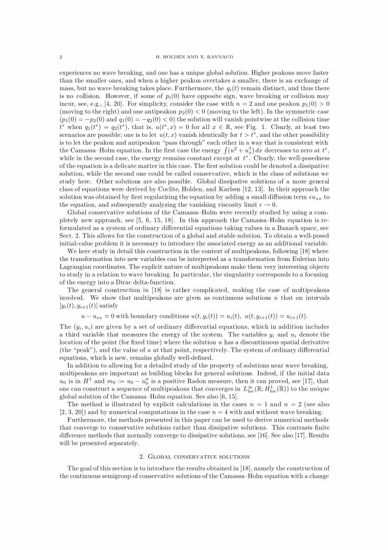
8/3/2019 Xavier Raynaud- On a Shallow Water Wave Equation
http://slidepdf.com/reader/full/xavier-raynaud-on-a-shallow-water-wave-equation 114/161
2 H. HOLDEN AND X. RAYNAUD
experiences no wave breaking, and one has a unique global solution. Higher peakons move fasterthan the smaller ones, and when a higher peakon overtakes a smaller, there is an exchange of mass, but no wave breaking takes place. Furthermore, the qi(t) remain distinct, and thus there
is no collision. However, if some of pi(0) have opposite sign, wave breaking or collision mayincur, see, e.g., [4, 20]. For simplicity, consider the case with n = 2 and one peakon p1(0) > 0(moving to the right) and one antipeakon p2(0) < 0 (moving to the left). In the symmetric case( p1(0) = − p2(0) and q1(0) = −q2(0) < 0) the solution will vanish pointwise at the collision timet∗ when q1(t∗) = q2(t∗), that is, u(t∗, x) = 0 for all x ∈ R, see Fig. 1. Clearly, at least twoscenarios are possible; one is to let u(t, x) vanish identically for t > t∗, and the other possibilityis to let the peakon and antipeakon “pass through” each other in a way that is consistent withthe Camassa–Holm equation. In the first case the energy
(u2 + u2
x) dx decreases to zero at t∗,while in the second case, the energy remains constant except at t∗. Clearly, the well-posednessof the equation is a delicate matter in this case. The first solution could be denoted a dissipativesolution, while the second one could be called conservative, which is the class of solutions westudy here. Other solutions are also possible. Global dissipative solutions of a more generalclass of equations were derived by Coclite, Holden, and Karlsen [12, 13]. In their approach thesolution was obtained by first regularizing the equation by adding a small diffusion term uxx tothe equation, and subsequently analyzing the vanishing viscosity limit → 0.
Global conservative solutions of the Camassa–Holm were recently studied by using a com-pletely new approach, see [5, 6, 15, 18]. In this approach the Camassa–Holm equation is re-formulated as a system of ordinary differential equations taking values in a Banach space, seeSect. 2. This allows for the construction of a global and stable solution. To obtain a well-posedinitial-value problem it is necessary to introduce the associated energy as an additional variable.
We here study in detail this construction in the context of multipeakons, following [18] wherethe transformation into new variables can be interpreted as a transformation from Eulerian intoLagrangian coordinates. The explicit nature of multipeakons make them very interesting objectsto study in a relation to wave breaking. In particular, the singularity corresponds to a focusingof the energy into a Dirac delta-function.
The general construction in [18] is rather complicated, making the case of multipeakonsinvolved. We show that multipeakons are given as continuous solutions u that on intervals[yi(t), yi+1(t)] satisfy
u − uxx = 0 with boundary conditions u(t, yi(t)) = ui(t), u(t, yi+1(t)) = ui+1(t).
The (yi, ui) are given by a set of ordinary differential equations, which in addition includesa third variable that measures the energy of the system. The variables yi and ui denote thelocation of the point (for fixed time) where the solution u has a discontinuous spatial derivative(the “peak”), and the value of u at that point, respectively. The system of ordinary differentialequations, which is new, remains globally well-defined.
In addition to allowing for a detailed study of the property of solutions near wave breaking,multipeakons are important as building blocks for general solutions. Indeed, if the initial datau0 is in H 1 and m0 := u0
−u
0
is a positive Radon measure, then it can proved, see [17], thatone can construct a sequence of multipeakons that converges in L∞
loc(R; H 1loc(R)) to the uniqueglobal solution of the Camassa–Holm equation. See also [6, 15].
The method is illustrated by explicit calculations in the cases n = 1 and n = 2 (see also[2, 3, 20]) and by numerical computations in the case n = 4 with and without wave breaking.
Furthermore, the methods presented in this paper can be used to derive numerical methodsthat converge to conservative solutions rather than dissipative solutions. This contrasts finitedifference methods that normally converge to dissipative solutions, see [16]. See also [17]. Resultswill be presented separately.
2. Global conservative solutions
The goal of this section is to introduce the results obtained in [18], namely the construction of the continuous semigroup of conservative solutions of the Camassa–Holm equation with a change
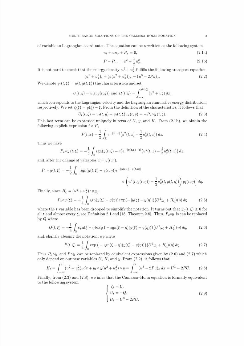
8/3/2019 Xavier Raynaud- On a Shallow Water Wave Equation
http://slidepdf.com/reader/full/xavier-raynaud-on-a-shallow-water-wave-equation 115/161
MULTIPEAKON SOLUTIONS OF THE CAMASSA–HOLM EQUATION 3
of variable to Lagrangian coordinates. The equation can be rewritten as the following system
ut + uux + P x = 0, (2.1a)
P − P xx = u2 + 12 u2x. (2.1b)
It is not hard to check that the energy density u2 + u2x fulfills the following transport equation
(u2 + u2x)t + (u(u2 + u2
x))x = (u3 − 2P u)x. (2.2)
We denote yt(t, ξ) = u(t, y(t, ξ)) the characteristics and set
U (t, ξ) = u(t, y(t, ξ)) and H (t, ξ) =
y(t,ξ)
−∞
(u2 + u2x) dx,
which corresponds to the Lagrangian velocity and the Lagrangian cumulative energy distribution,respectively. We set ζ (ξ) = y(ξ) − ξ. From the definition of the characteristics, it follows that
U t(t, ξ) = ut(t, y) + yt(t, ξ)ux(t, y) = −P x◦y (t, ξ). (2.3)
This last term can be expressed uniquely in term of U , y, and H . From (2.1b), we obtain thefollowing explicit expression for P ,
P (t, x) =1
2
R
e−|x−z|
u2(t, z) +1
2u2x(t, z)
dz. (2.4)
Thus we have
P x◦y (t, ξ) = − 1
2
R
sgn(y(t, ξ) − z)e−|y(t,ξ)−z|
u2(t, z) +1
2u2x(t, z)
dz,
and, after the change of variables z = y(t, η),
P x ◦ y(t, ξ) = − 1
2
R
sgn(y(t, ξ) − y(t, η))e−|y(t,ξ)−y(t,η)|
× u
2
(t, y(t, η)) +1
2 u2x(t, y(t, η))
yξ(t, η)
dη.
Finally, since H ξ = (u2 + u2x)◦y yξ,
P x◦y (ξ) = − 1
4
R
sgn(y(ξ) − y(η))exp(− |y(ξ) − y(η)|)U 2yξ + H ξ
(η) dη (2.5)
where the t variable has been dropped to simplify the notation. It turns out that yξ(t, ξ) ≥ 0 forall t and almost every ξ, see Definition 2.1 and [18, Theorem 2.8]. Thus, P x◦y is can be replacedby Q where
Q(t, ξ) = − 1
4
R
sgn(ξ − η)exp− sgn(ξ − η)(y(ξ) − y(η))
U 2yξ + H ξ
(η) dη, (2.6)
and, slightly abusing the notation, we write
P (t, ξ) = 14
R
exp− sgn(ξ − η)(y(ξ) − y(η))
U 2yξ + H ξ
(η) dη. (2.7)
Thus P x◦y and P ◦y can be replaced by equivalent expressions given by (2.6) and (2.7) whichonly depend on our new variables U , H , and y. From (2.2), it follows that
H t =
y−∞
(u2 + u2x)t dx + yt ◦ y(u2 + u2
x) ◦ y =
y−∞
(u3 − 2P u)x dx = U 3 − 2P U. (2.8)
Finally, from (2.3) and (2.8), we infer that the Camassa–Holm equation is formally equivalentto the following system
ζ t = U,
U t = −Q,
H t = U 3
−2P U.
(2.9)
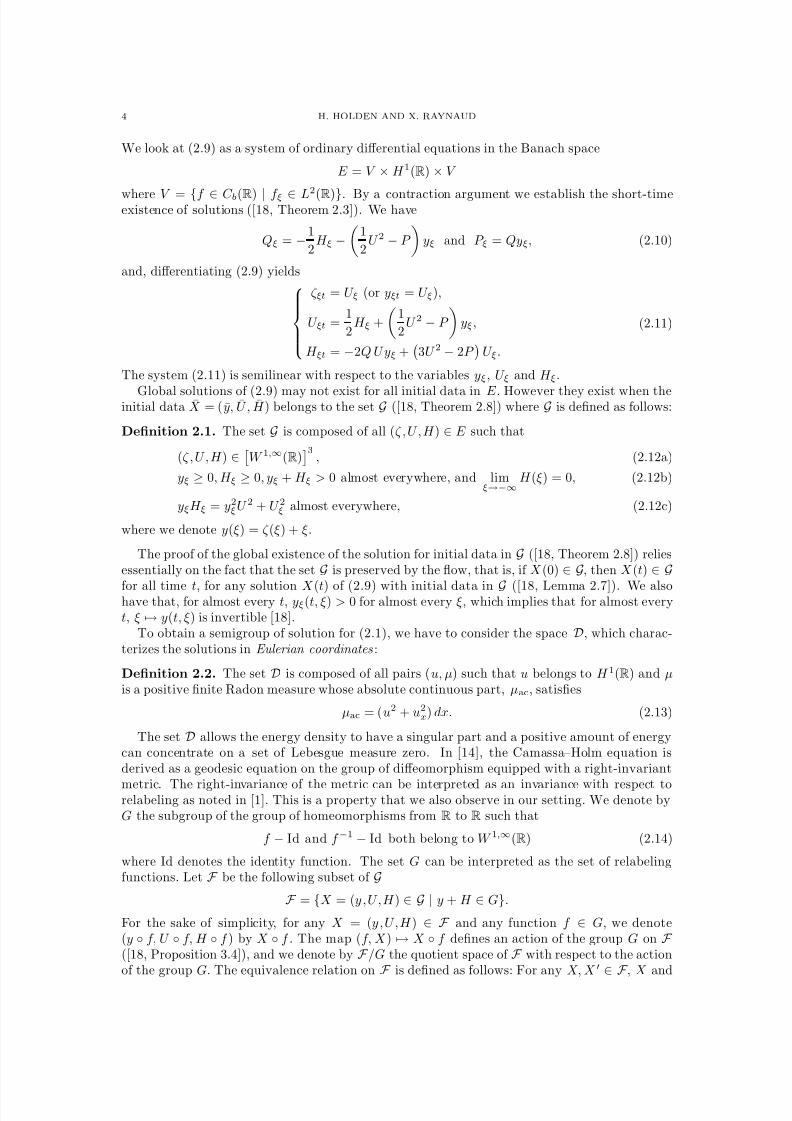
8/3/2019 Xavier Raynaud- On a Shallow Water Wave Equation
http://slidepdf.com/reader/full/xavier-raynaud-on-a-shallow-water-wave-equation 116/161
4 H. HOLDEN AND X. RAYNAUD
We look at (2.9) as a system of ordinary differential equations in the Banach space
E = V × H 1(R) × V
where V = {f ∈ C b(R) | f ξ ∈ L2
(R)}. By a contraction argument we establish the short-timeexistence of solutions ([18, Theorem 2.3]). We have
Qξ = −1
2H ξ −
1
2U 2 − P
yξ and P ξ = Qyξ, (2.10)
and, differentiating (2.9) yields
ζ ξt = U ξ (or yξt = U ξ),
U ξt =1
2H ξ +
1
2U 2 − P
yξ,
H ξt = −2Q U yξ +
3U 2 − 2P
U ξ.
(2.11)
The system (2.11) is semilinear with respect to the variables yξ, U ξ and H ξ.
Global solutions of (2.9) may not exist for all initial data in E . However they exist when theinitial data X = (y, U , H ) belongs to the set G ([18, Theorem 2.8]) where G is defined as follows:
Definition 2.1. The set G is composed of all (ζ , U , H ) ∈ E such that
(ζ , U , H ) ∈ W 1,∞(R)
3, (2.12a)
yξ ≥ 0, H ξ ≥ 0, yξ + H ξ > 0 almost everywhere, and limξ→−∞
H (ξ) = 0, (2.12b)
yξH ξ = y2ξU 2 + U 2ξ almost everywhere, (2.12c)
where we denote y(ξ) = ζ (ξ) + ξ.
The proof of the global existence of the solution for initial data in G ([18, Theorem 2.8]) reliesessentially on the fact that the set G is preserved by the flow, that is, if X (0) ∈ G, then X (t) ∈ Gfor all time t, for any solution X (t) of (2.9) with initial data in G ([18, Lemma 2.7]). We alsohave that, for almost every t, yξ(t, ξ) > 0 for almost every ξ, which implies that for almost everyt, ξ → y(t, ξ) is invertible [18].
To obtain a semigroup of solution for (2.1), we have to consider the space D, which charac-terizes the solutions in Eulerian coordinates:
Definition 2.2. The set D is composed of all pairs (u, µ) such that u belongs to H 1(R) and µis a positive finite Radon measure whose absolute continuous part, µac, satisfies
µac = (u2 + u2x) dx. (2.13)
The set D allows the energy density to have a singular part and a positive amount of energycan concentrate on a set of Lebesgue measure zero. In [14], the Camassa–Holm equation isderived as a geodesic equation on the group of diffeomorphism equipped with a right-invariant
metric. The right-invariance of the metric can be interpreted as an invariance with respect torelabeling as noted in [1]. This is a property that we also observe in our setting. We denote byG the subgroup of the group of homeomorphisms from R to R such that
f − Id and f −1 − Id both belong to W 1,∞(R) (2.14)
where Id denotes the identity function. The set G can be interpreted as the set of relabelingfunctions. Let F be the following subset of G
F = {X = (y,U,H ) ∈ G | y + H ∈ G}.
For the sake of simplicity, for any X = (y,U,H ) ∈ F and any function f ∈ G, we denote(y ◦ f, U ◦ f, H ◦ f ) by X ◦ f . The map (f, X ) → X ◦ f defines an action of the group G on F ([18, Proposition 3.4]), and we denote by F /G the quotient space of F with respect to the actionof the group G. The equivalence relation on
F is defined as follows: For any X, X
∈ F , X and
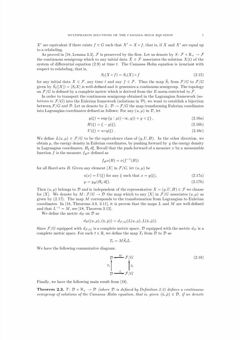
8/3/2019 Xavier Raynaud- On a Shallow Water Wave Equation
http://slidepdf.com/reader/full/xavier-raynaud-on-a-shallow-water-wave-equation 117/161
MULTIPEAKON SOLUTIONS OF THE CAMASSA–HOLM EQUATION 5
X are equivalent if there exists f ∈ G such that X = X ◦ f , that is, if X and X are equal upto a relabeling.
As proved in [18, Lemma 3.3],
F is preserved by the flow. Let us denote by S :
F ×R+
→ F the continuous semigroup which to any initial data X ∈ F associates the solution X (t) of thesystem of differential equation (2.9) at time t. The Camassa–Holm equation is invariant withrespect to relabeling, that is,
S t(X ◦ f ) = S t(X ) ◦ f (2.15)
for any initial data X ∈ F , any time t and any f ∈ F . Thus the map S t from F /G to F /Ggiven by S t([X ]) = [S tX ] is well-defined and it generates a continuous semigroup. The topologyon F /G is defined by a complete metric which is derived from the E -norm restricted to F .
In order to transport the continuous semigroup obtained in the Lagrangian framework (so-lutions in F /G) into the Eulerian framework (solutions in D), we want to establish a bijectionbetween F /G and D. Let us denote by L : D → F /G the map transforming Eulerian coordinatesinto Lagrangian coordinates defined as follows: For any (u, µ) in D, let
y(ξ) = sup {y | µ((−∞, y)) + y < ξ} , (2.16a)H (ξ) = ξ − y(ξ), (2.16b)
U (ξ) = u◦y(ξ) . (2.16c)
We define L(u, µ) ∈ F /G to be the equivalence class of (y,U,H ). In the other direction, weobtain µ, the energy density in Eulerian coordinates, by pushing forward by y the energy densityin Lagrangian coordinates, H ξ dξ. Recall that the push-forward of a measure ν by a measurablefunction f is the measure f #ν defined as
f #ν (B) = ν (f −1(B))
for all Borel sets B. Given any element [X ] in F /G, let (u, µ) be
u(x) = U (ξ) for any ξ such that x = y(ξ), (2.17a)
µ = y#(H ξ dξ). (2.17b)
Then (u, µ) belongs to D and is independent of the representative X = (y,U,H ) ∈ F we choosefor [X ]. We denote by M : F /G → D the map which to any [X ] in F /G associates (u, µ) asgiven by (2.17). The map M corresponds to the transformation from Lagrangian to Euleriancoordinates. In [18, Theorems 3.8, 3.11], it is proven that the maps L and M are well-definedand that L−1 = M , see [18, Theorem 3.12].
We define the metric dD on D as
dD((u, µ), (u, µ)) = dF /G(L(u, µ), L(u, µ)).
Since F /G equipped with dF /G is a complete metric space, D equipped with the metric dD is acomplete metric space. For each t ∈ R, we define the map T t from D to D as
T t = M S tL.
We have the following commutative diagram:
D F /GM o o
D
T t
O O
L / / F /G
St
O O(2.18)
Finally, we have the following main result from [18].
Theorem 2.3. T : D × R+ → D (where D is defined by Definition 2.2) defines a continuoussemigroup of solutions of the Camassa–Holm equation, that is, given (u, µ)
∈ D, if we denote
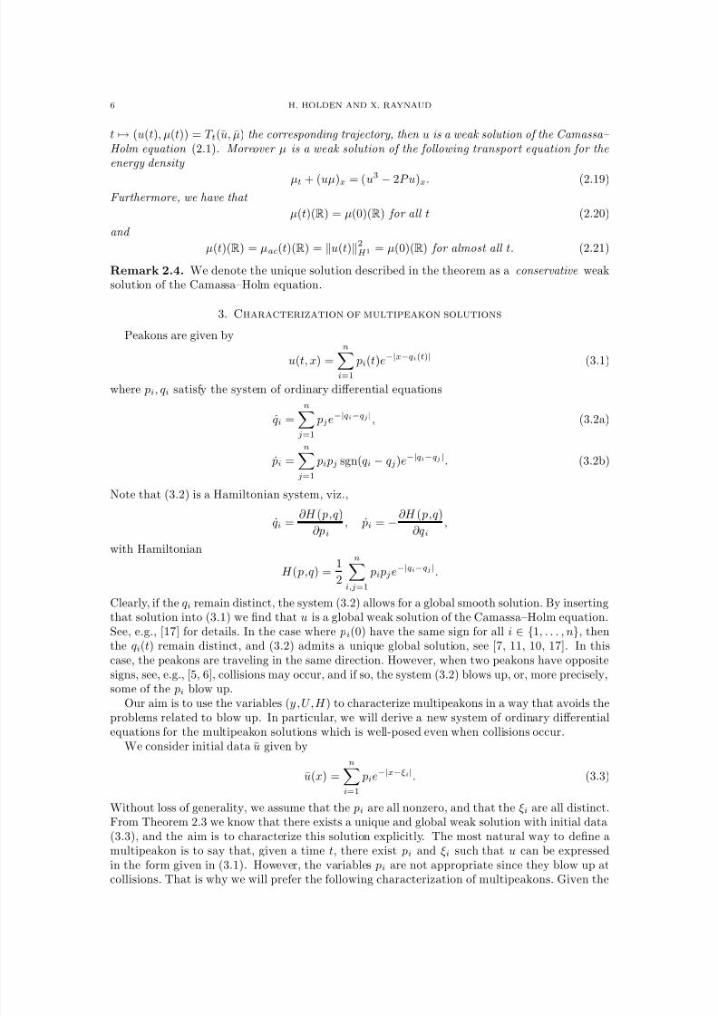
8/3/2019 Xavier Raynaud- On a Shallow Water Wave Equation
http://slidepdf.com/reader/full/xavier-raynaud-on-a-shallow-water-wave-equation 118/161
6 H. HOLDEN AND X. RAYNAUD
t → (u(t), µ(t)) = T t(u, µ) the corresponding trajectory, then u is a weak solution of the Camassa– Holm equation (2.1). Moreover µ is a weak solution of the following transport equation for theenergy density
µt + (uµ)x = (u3 − 2P u)x. (2.19)Furthermore, we have that
µ(t)(R) = µ(0)(R) for all t (2.20)
and
µ(t)(R) = µac(t)(R) = u(t)2H 1 = µ(0)(R) for almost all t. (2.21)
Remark 2.4. We denote the unique solution described in the theorem as a conservative weaksolution of the Camassa–Holm equation.
3. Characterization of multipeakon solutions
Peakons are given by
u(t, x) =
ni=1
pi(t)e−|x−qi(t)| (3.1)
where pi, qi satisfy the system of ordinary differential equations
qi =
nj=1
pje−|qi−qj |, (3.2a)
˙ pi =
nj=1
pi pj sgn(qi − qj)e−|qi−qj |. (3.2b)
Note that (3.2) is a Hamiltonian system, viz.,
qi =∂H ( p,q)
∂pi, ˙ pi =
−∂H ( p,q)
∂qi,
with Hamiltonian
H ( p,q) =1
2
ni,j=1
pi pje−|qi−qj |.
Clearly, if the qi remain distinct, the system (3.2) allows for a global smooth solution. By insertingthat solution into (3.1) we find that u is a global weak solution of the Camassa–Holm equation.See, e.g., [17] for details. In the case where pi(0) have the same sign for all i ∈ {1, . . . , n}, thenthe qi(t) remain distinct, and (3.2) admits a unique global solution, see [7, 11, 10, 17]. In thiscase, the peakons are traveling in the same direction. However, when two peakons have oppositesigns, see, e.g., [5, 6], collisions may occur, and if so, the system (3.2) blows up, or, more precisely,some of the pi blow up.
Our aim is to use the variables (y,U,H ) to characterize multipeakons in a way that avoids theproblems related to blow up. In particular, we will derive a new system of ordinary differentialequations for the multipeakon solutions which is well-posed even when collisions occur.
We consider initial data u given by
u(x) =ni=1
pie−|x−ξi|. (3.3)
Without loss of generality, we assume that the pi are all nonzero, and that the ξi are all distinct.From Theorem 2.3 we know that there exists a unique and global weak solution with initial data(3.3), and the aim is to characterize this solution explicitly. The most natural way to define amultipeakon is to say that, given a time t, there exist pi and ξi such that u can be expressedin the form given in (3.1). However, the variables pi are not appropriate since they blow up atcollisions. That is why we will prefer the following characterization of multipeakons. Given the
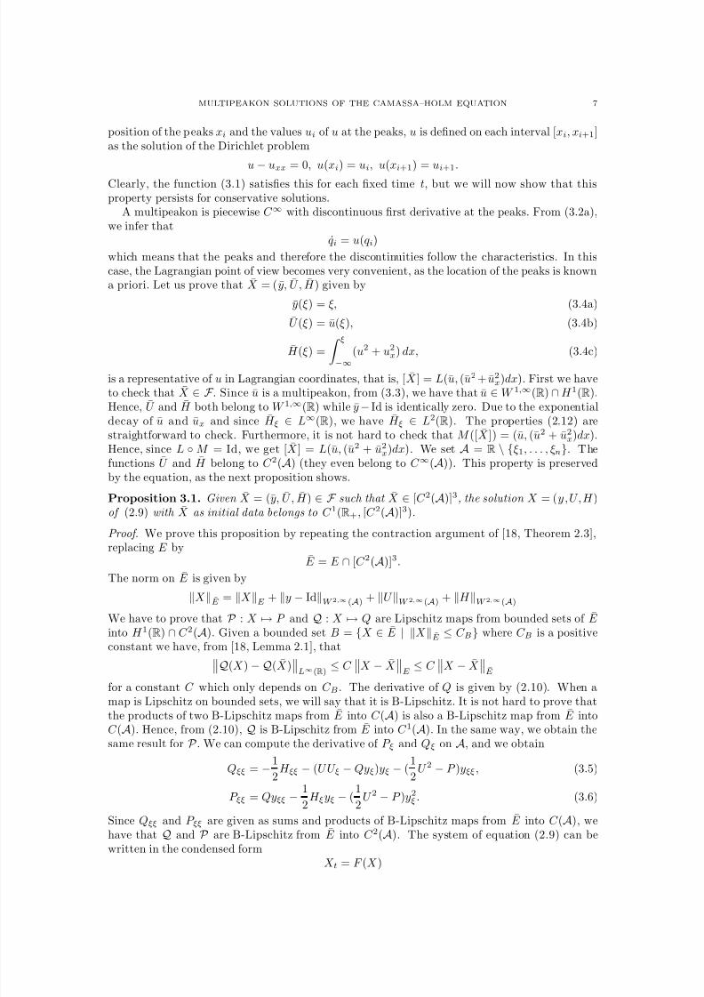
8/3/2019 Xavier Raynaud- On a Shallow Water Wave Equation
http://slidepdf.com/reader/full/xavier-raynaud-on-a-shallow-water-wave-equation 119/161
MULTIPEAKON SOLUTIONS OF THE CAMASSA–HOLM EQUATION 7
position of the peaks xi and the values ui of u at the peaks, u is defined on each interval [xi, xi+1]as the solution of the Dirichlet problem
u
−uxx = 0, u(xi) = ui, u(xi+1) = ui+1.
Clearly, the function (3.1) satisfies this for each fixed time t, but we will now show that thisproperty persists for conservative solutions.
A multipeakon is piecewise C ∞ with discontinuous first derivative at the peaks. From (3.2a),we infer that
qi = u(qi)
which means that the peaks and therefore the discontinuities follow the characteristics. In thiscase, the Lagrangian point of view becomes very convenient, as the location of the peaks is knowna priori. Let us prove that X = (y, U , H ) given by
y(ξ) = ξ, (3.4a)
U (ξ) = u(ξ), (3.4b)
H (ξ) = ξ−∞
(u2 + u2x) dx, (3.4c)
is a representative of u in Lagrangian coordinates, that is, [X ] = L(u, (u2 + u2x)dx). First we have
to check that X ∈ F . Since u is a multipeakon, from (3.3), we have that u ∈ W 1,∞(R) ∩ H 1(R).Hence, U and H both belong to W 1,∞(R) while y − Id is identically zero. Due to the exponentialdecay of u and ux and since H ξ ∈ L∞(R), we have H ξ ∈ L2(R). The properties (2.12) arestraightforward to check. Furthermore, it is not hard to check that M ([X ]) = (u, (u2 + u2
x)dx).Hence, since L ◦ M = Id, we get [X ] = L(u, (u2 + u2
x)dx). We set A = R \ {ξ1, . . . , ξn}. Thefunctions U and H belong to C 2(A) (they even belong to C ∞(A)). This property is preservedby the equation, as the next proposition shows.
Proposition 3.1. Given X = (y, U , H ) ∈ F such that X ∈ [C 2(A)]3, the solution X = (y,U,H )of (2.9) with X as initial data belongs to C 1(R+, [C 2(
A)]3).
Proof. We prove this proposition by repeating the contraction argument of [18, Theorem 2.3],replacing E by
E = E ∩ [C 2(A)]3.
The norm on E is given by
X E = X E + y − IdW 2,∞(A) + U W 2,∞(A) + H W 2,∞(A)
We have to prove that P : X → P and Q : X → Q are Lipschitz maps from bounded sets of E into H 1(R) ∩ C 2(A). Given a bounded set B = {X ∈ E | X E ≤ C B} where C B is a positiveconstant we have, from [18, Lemma 2.1], that
Q(X ) − Q(X )
L∞(R)
≤ C
X − X E
≤ C
X − X E
for a constant C which only depends on C B. The derivative of Q is given by (2.10). When a
map is Lipschitz on bounded sets, we will say that it is B-Lipschitz. It is not hard to prove thatthe products of two B-Lipschitz maps from E into C (A) is also a B-Lipschitz map from E intoC (A). Hence, from (2.10), Q is B-Lipschitz from E into C 1(A). In the same way, we obtain thesame result for P . We can compute the derivative of P ξ and Qξ on A, and we obtain
Qξξ = −1
2H ξξ − (U U ξ − Qyξ)yξ − (
1
2U 2 − P )yξξ , (3.5)
P ξξ = Qyξξ − 1
2H ξyξ − (
1
2U 2 − P )y2
ξ . (3.6)
Since Qξξ and P ξξ are given as sums and products of B-Lipschitz maps from E into C (A), wehave that Q and P are B-Lipschitz from E into C 2(A). The system of equation (2.9) can bewritten in the condensed form
X t = F (X )
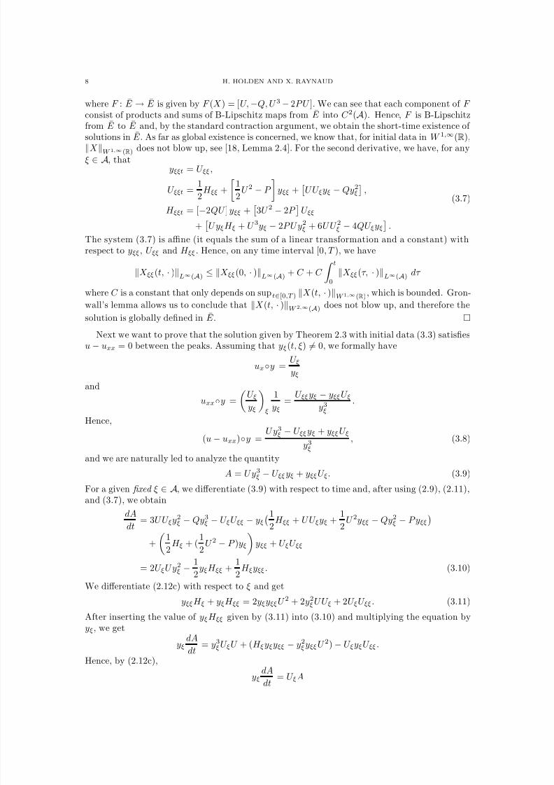
8/3/2019 Xavier Raynaud- On a Shallow Water Wave Equation
http://slidepdf.com/reader/full/xavier-raynaud-on-a-shallow-water-wave-equation 120/161
8 H. HOLDEN AND X. RAYNAUD
where F : E → E is given by F (X ) = [U, −Q, U 3 − 2P U ]. We can see that each component of F consist of products and sums of B-Lipschitz maps from E into C 2(A). Hence, F is B-Lipschitzfrom E to E and, by the standard contraction argument, we obtain the short-time existence of
solutions in E . As far as global existence is concerned, we know that, for initial data in W 1,∞(R),X W 1,∞(R) does not blow up, see [18, Lemma 2.4]. For the second derivative, we have, for any
ξ ∈ A, thatyξξt = U ξξ ,
U ξξt =1
2H ξξ +
1
2U 2 − P
yξξ +
U U ξyξ − Qy2
ξ
,
H ξξt = [−2QU ] yξξ +
3U 2 − 2P
U ξξ
+
U yξH ξ + U 3yξ − 2P U y2ξ + 6U U 2ξ − 4QU ξyξ
.
(3.7)
The system (3.7) is affine (it equals the sum of a linear transformation and a constant) withrespect to yξξ , U ξξ and H ξξ . Hence, on any time interval [0, T ), we have
X ξξ(t, · )L∞(A) ≤ X ξξ(0, · )L∞(A) + C + C t
0 X ξξ(τ, · )L∞(A) dτ
where C is a constant that only depends on sup t∈[0,T ) X (t, · )W 1,∞(R), which is bounded. Gron-
wall’s lemma allows us to conclude that X (t, · )W 2,∞(A) does not blow up, and therefore the
solution is globally defined in E .
Next we want to prove that the solution given by Theorem 2.3 with initial data (3.3) satisfiesu − uxx = 0 between the peaks. Assuming that yξ(t, ξ) = 0, we formally have
ux◦y =U ξyξ
and
uxx◦y = U ξyξξ
1
yξ
=U ξξyξ − yξξU ξ
y3
ξ
.
Hence,
(u − uxx)◦y =U y3
ξ − U ξξyξ + yξξU ξ
y3ξ
, (3.8)
and we are naturally led to analyze the quantity
A = U y3ξ − U ξξyξ + yξξU ξ. (3.9)
For a given fixed ξ ∈ A, we differentiate (3.9) with respect to time and, after using (2.9), (2.11),and (3.7), we obtain
dA
dt= 3U U ξy2
ξ − Qy3ξ − U ξU ξξ − yξ
1
2H ξξ + U U ξyξ +
1
2U 2yξξ − Qy2
ξ − P yξξ
+ 1
2H ξ + (
1
2U 2
−P )yξ yξξ + U ξU ξξ
= 2U ξU y2ξ − 1
2yξH ξξ +
1
2H ξyξξ . (3.10)
We differentiate (2.12c) with respect to ξ and get
yξξH ξ + yξH ξξ = 2yξyξξU 2 + 2y2ξU U ξ + 2U ξU ξξ . (3.11)
After inserting the value of yξH ξξ given by (3.11) into (3.10) and multiplying the equation byyξ, we get
yξdA
dt= y3
ξU ξU + (H ξyξyξξ − y2ξyξξU 2) − U ξyξU ξξ .
Hence, by (2.12c),
yξdA
dt
= U ξA
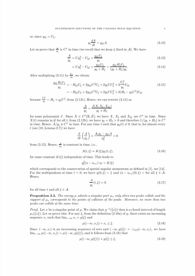
8/3/2019 Xavier Raynaud- On a Shallow Water Wave Equation
http://slidepdf.com/reader/full/xavier-raynaud-on-a-shallow-water-wave-equation 121/161
MULTIPEAKON SOLUTIONS OF THE CAMASSA–HOLM EQUATION 9
or, since yξt = U ξ,
yξdA
dt= yξtA. (3.12)
Let us prove that Ayξ
is C 1 in time (we recall that we keep ξ fixed in A). We have
A
yξ= U y2
ξ − U ξξ +yξξU ξ
yξ(3.13)
= U y2ξ − U ξξ +
yξξU ξyξ + H ξ
+yξξH ξU ξ
(yξ + H ξ)yξ. (3.14)
After multiplying (3.11) byU ξyξ
, we obtain
yξξH ξU ξyξ
= −H ξξU ξ + 2yξξU 2U ξ + 2yξU U 2ξ + 2U 2ξyξ
U ξξ (3.15)
= −H ξξU ξ + 2yξξU 2U ξ + 2yξU U 2ξ + 2(H ξ − yξU 2)U ξξ
becauseU 2ξyξ
= H ξ + yξU 2, from (2.12c). Hence, we can rewrite (3.14) as
A
yξ=
J (X, X ξ, X ξξ)
yξ + H ξ
for some polynomial J . Since X ∈ C 1(R, E ), we have X , X ξ and X ξξ are C 1 in time. SinceX (t) remains in G for all t, from (2.12b), we have yξ + H ξ > 0 and therefore 1/(yξ + H ξ) is C 1
in time. Hence, A/yξ is C 1 in time. For any time t such that yξ(t) = 0, that is, for almost everyt (see [18, Lemma 2.7]) we have
d
dt
A
yξ
=
Atyξ − yξtA
y2ξ
= 0
from (3.12). Hence,Ayξ is constant in time, i.e.,
A(t, ξ) = K (ξ)yξ(t, ξ), (3.16)
for some constant K (ξ) independent of time. This leads to
y2ξ(u − uxx)◦y = K (ξ)
which corresponds to the conservation of spatial angular momentum as defined in [1], see [14].For the multipeakons at time t = 0, we have y(0, ξ) = ξ and (u − uxx)(0, ξ) = for all ξ ∈ A.Hence,
A
yξ(t, ξ) = 0 (3.17)
for all time t and all ξ
∈ A.
Proposition 3.2. The energy µ admits a singular part µs only when two peaks collide and thesupport of µs corresponds to the points of collision of the peaks. Moreover, no more than twopeaks can collide at the same time.
Proof. Let x be a singular point of µ. We claim that y−1({x}) then is a closed interval of lengthµs({x}). Let us prove this. For any ξ, from the definition (2.16a) of y, there exists an increasingsequence xi such that limi→∞ xi = y(ξ) and
µ((−∞, xi)) + xi ≤ ξ. (3.18)
Since (−∞, xi) is an increasing sequence of sets and (−∞, y(ξ)) = ∪i∈N(−∞, xi), we havelimi→∞ µ((−∞, xi)) = µ((−∞, y(ξ))), and it follows from (3.18) that
µ((
−∞, y(ξ))) + y(ξ)
≤ξ. (3.19)
8/3/2019 Xavier Raynaud- On a Shallow Water Wave Equation
http://slidepdf.com/reader/full/xavier-raynaud-on-a-shallow-water-wave-equation 122/161
10 H. HOLDEN AND X. RAYNAUD
We set ξ = µ((−∞, x)) +x and, using (3.19), it is not hard to prove that ξ is the smallest elementof y−1({x}). Let ξ ∈ y−1({x}), by definition of y, there exists a decreasing sequence xi whichconverges to x such that
µ((−∞, xi)) + xi > ξ.Letting i tend to infinity, we obtain
ξ ≤ µ((−∞, x]) + x
≤ µ((−∞, x)) + µs({x}) + x
≤ ξ + µs({x}).
Hence, ξ ∈ [ξ, ξ + µs({x})] and y−1({x}) ⊂ [ξ, ξ + µs({x})]. Conversely, let us consider ξ ∈[ξ, ξ + µs({x})]. Since y is increasing, y(ξ) ≥ y(ξ) = x. Assume that y(ξ) > x. Then, it followsfrom the definition of y that there exists x > x such that
µ((−∞), x) + x ≤ ξ.
Since x
> x, we haveµ((−∞, x)) ≥ µ((−∞, x])
= µ((−∞, x)) + µs({x})
= ξ − x + µs({x}).
Hence, ξ − x + µs({x}) + x ≤ ξ which implies ξ + µs({x}) < ξ. This contradicts the fact thatξ ∈ [ξ, ξ + µs({x})]. Our claim is proved. This claim is a general result and does not dependon the multipeakon structure of the initial data. For solutions with multipeakon initial data, wehave the following result.
Lemma 3.3. If yξ(t, ξ) vanishes at some point ξ in the interval (ξi, ξi+1), then yξ(t, ξ) vanisheseverywhere in (ξi, ξi+1).
Proof of Lemma 3.3. Let B be the set
B = {ξ ∈ (ξi, ξi+1) | yξ(t, ξ) = 0} .
The set B is not empty as ξ ∈ B. Since yξ(t, · ) ∈ C (A), B is closed (relatively in (ξi, ξi+1)).Let us prove that B is also open. Take a point ξ0 ∈ B. We have yξ(t, ξ0) = 0 and, by (2.12b),it implies H ξ(t, ξ0) > 0. Since H ξ(t, · ) ∈ C (A), there exists an open interval I around ξ0 suchthat H ξ(t, ξ) > 0 for all ξ ∈ I . After multiplying (3.17) by U ξ and using (2.12c), we obtain
U U ξy2ξ − U ξU ξξ + yξξH ξ − yξξyξU 2 = 0. (3.20)
We differentiate (2.12c) with respect to ξ and obtain
U ξξU ξ =1
2(yξξH ξ + H ξξyξ) − yξyξξU 2 − y2
ξU ξU. (3.21)
Inserting this into (3.20), we end up with an equation of the form
yξξH ξ = f (ξ)yξ (3.22)
where f (ξ) is a continuous function of ξ. Since H ξ = 0 on I , we obtain
yξξ(ξ) =f (ξ)
H ξ(ξ)yξ(ξ),
yξ(ξ0) = 0.
The unique solution of this ordinary differential equation where yξ(ξ) plays the role of the un-known, is yξ(ξ) = 0. Hence, yξ(ξ) = 0 for all ξ ∈ I . This implies that I ⊂ B and therefore B isopen. Thus B is an open and closed set, relatively in (ξi, ξi+1). Since (ξi, ξi+1) is a connectedset, it implies that B = (ξi, ξi+1), which concludes the proof of the lemma.
8/3/2019 Xavier Raynaud- On a Shallow Water Wave Equation
http://slidepdf.com/reader/full/xavier-raynaud-on-a-shallow-water-wave-equation 123/161
MULTIPEAKON SOLUTIONS OF THE CAMASSA–HOLM EQUATION 11
Let us consider a time T when µ admits a singular point that we denote {x}. Then, theinterval of strictly positive length y−1({x}) intersects A and there exists a point ξ ∈ (ξi, ξi+1)for some i
∈ {1, . . . , n
}such that yξ(T, ξ) = 0 (with the convention ξ0 =
−∞and ξn+1 =
∞).
From Lemma 3.3, we get that [ξi, ξi+1] ⊂ y−1({x}). In particular, y(ξi) = y(ξi+1) = x, whichmeans that the point x where the energy concentrates, is located at the collision point betweentwo peaks. We claim that
[ξi, ξi+1] = y−1({x}), (3.23)
which in particular means that no other peak than the ones originating from ξi and ξi+1 can befound at x. Assume that (3.23) is not true, then, due to Lemma 3.3, y−1({x}) must take theform
y−1({x}) = [ξj, ξk]
where j ≤ i, k ≥ i + 1 and k − j ≥ 2. We introduce X = (y, U , H ) defined as y(ξ) = y(T, ξ),U (ξ) = U (T, ξ), and
H (ξ) =H (T, ξj)
ξk − ξ
ξk − ξj+ H (T, ξk)
ξ − ξj
ξk − ξjwhen ξ
∈(ξj , ξk),
H (T, ξ) otherwise,
so that H is linear in (ξj , ξk) and continuous. Since yξ(T, ξ) = U ξ(T, ξ) = 0 and H ξ(T, ξ) > 0 in(ξj , ξj), it is not hard to check that all the conditions (2.12) are fulfilled and X ∈ F . Let us lookat X (T ) and X in Eulerian coordinates. We write (u, µ) = M ([X (T )]) and (u, µ) = M ([X ]).Since y(ξ) = y(T, ξ) and U (ξ) = U (T, ξ), it is clear that u = u. We have, using (2.17b),
µ({x}) =
[ξj ,ξk]
H ξ dξ = H (ξk) − H (ξj) =
[ξj ,ξk]
H ξ dξ = µ({x}).
Hence, for any Borel set A,
µ(A) = µ(A \ {x}) + µ({x}) = µ(A \ {x}) + µ({x}) = µ(A)
and µ = µ. Since M is injective, we have [X (T )] = [X ], which means that X (T ) and X areequivalent and there exists f ∈ F such that
X (T ) ◦ f = X. (3.24)
The point is that X is linear in (ξj , ξk), and therefore it possesses a priori more regularity than
X (T ) on this interval. Introduce A = R\{ξ1, . . . , ξj , ξk, . . . , ξn}. We can solve (2.9) backward intime and, slightly abusing the notation, we denote X (t) the solution which satisfies X (T ) = X
at time T . Proposition 3.1 gives us that X (t) ∈ [C 2(A)]3 for all time t. Since X (T ) and X (T )are equivalent and satisfy (3.24), by (2.15), we obtain that X (t) ◦ f = X (t) for all time t. Attime t = 0, it yields
f (ξ) = y(0, ξ)
because y(0, ξ) = ξ. Since y(0, ξ)
∈C 2((ξj , ξk)), f
∈C 2((ξj , ξk)). By definition, see (2.14), the
derivative of f −1 is bounded. It implies that f ξ is bounded strictly away from zero, see [18,Lemma 3.2] for a detailed proof of this result. Hence, f ξ > 0 in (ξj , ξk) and, by the implicitfunction theorem, f −1 belongs to C 2((ξj , ξk)). Hence,
u(0, ξ) = U (0, ξ) = U (0, f −1(ξ))
also belongs to C 2((ξj, ξk)). This contradicts the fact that (ξj , ξk) contains either ξi or ξi+1,which are points where the derivative of u(0, ξ) is discontinuous.
Given (t, x) ∈ R+ × R, there exists ξ, which may not be unique, such that x = y(t, ξ). If ξ ∈ Ac, then x corresponds to the position of a peak. For ξ ∈ A, if yξ(t, ξ) = 0, then, by Lemma3.3, yξ(t, ξ) = 0 for all ξ ∈ (ξi, ξi+1) where i is such that ξ ∈ (ξi, ξi+1), and x again correspondsto a peak. If yξ(t, ξ) = 0 then, using again Lemma 3.3, we have yξ(t, ξ) = 0 for all ξ ∈ (ξi, ξi+1).By the implicit function theorem, we obtain that y(t,
·) is invertible in (ξi, ξi+1) and its inverse
8/3/2019 Xavier Raynaud- On a Shallow Water Wave Equation
http://slidepdf.com/reader/full/xavier-raynaud-on-a-shallow-water-wave-equation 124/161
12 H. HOLDEN AND X. RAYNAUD
is C 2. It follows that u(t, x) = U (t, y−1(t, x)) is C 2 with respect to the spatial variable and thequantity (u − uxx)(t, x) is defined in the classical sense. Moreover, by (3.17) and (3.8), we have
(u − uxx)(t, x) =
A(t, ξ)
y3ξ (t, ξ) = 0. (3.25)
We summarize our results in the following theorem.
Theorem 3.4. Given an initial multipeakon solution u(x) =n
i=1 pie−|x−ξi|, let (y,U,H ) be the
solution of the system (2.9) with initial data (y, U , H ) given by (3.4). Between adjacent peaks,say xi = y(t, ξi) = xi+1 = y(t, ξi+1), the solution u(t, x) is twice differentiable with respect to thespace variable, and we have
(u − uxx)(t, x) = 0 for x ∈ (xi, xi+1).
We are now in position to start the derivation of a system of ordinary differential equationsfor multipeakons.
4. A system of ordinary differential equations for multipeakonsFor each i ∈ {1, . . . , n}, we have, from (2.9),
dyidt
= ui,
duidt
= −Qi,
dH idt
= u3i − 2P iui
(4.1)
where yi, ui, H i, P i and Qi denote y(t, ξi), U (t, ξi), H (t, ξi), P (t, ξi) and Q(t, ξi), respectively. Foralmost every t, the function y(t, · ) is invertible. We can make the change of variables x = y(t, ξ)so that P i and Qi can be rewritten as
P i =1
2 R
e−|yi−x|(u2 +1
2 u2x) dx, (4.2)
Qi = −1
2
R
sgn(yi − x)e−|yi−x|(u2 +1
2u2x) dx. (4.3)
Theorem 3.4 gives us a priori the shape of u and allows us to express P i and Qi as a functionof the variables ui, H i and yi only, thereby transforming (4.1) into a well-posed 3n-dimensionalsystem of ordinary differential equations.
For almost every time t, yξ(t, ξ) > 0 for almost every ξ and ξ → y(t, ξ) is invertible, see Sect.2 . From now on, we will consider such time t and omit it in the notation when there is noambiguity. For such time, by Theorem 3.4, no peak coincide. From the same theorem, we knowthat between two adjacent peaks located at yi and yi+1, u satisfies u − uxx = 0 and therefore ucan be written as
u(x) = Aiex + Bie−x for x ∈ [yi, yi+1], i = 1, . . . , n − 1. (4.4)
The constants Ai and Bi depend on ui, ui+1, yi and yi+1 and read
Ai =e−yi
2
ui
cosh(δyi)+
δuisinh(δyi)
, (4.5)
Bi =eyi
2
ui
cosh(δyi)− δui
sinh(δyi)
, (4.6)
where we for convenience have introduced the variables
yi =1
2(yi + yi+1), δyi =
1
2(yi+1 − yi), (4.7)
ui =1
2(ui + ui+1), δui =
1
2(ui+1 − ui).
8/3/2019 Xavier Raynaud- On a Shallow Water Wave Equation
http://slidepdf.com/reader/full/xavier-raynaud-on-a-shallow-water-wave-equation 125/161
MULTIPEAKON SOLUTIONS OF THE CAMASSA–HOLM EQUATION 13
The constants Ai and Bi uniquely determine u on the interval [yi, yi+1]. Thus, we can compute
δH i = H i+1 − H i = yi+1
yi
(u2 + u2x) dx
= 2u2i tanh(δyi) + 2δu2
i coth(δyi). (4.8)
At this point, we can get some more understanding of what is happening at a time of collision. Lett∗ be a time when the two peaks located at yi and yi+1 collide, i.e., such that limt↑t∗ δyi(t) = 0.Since the solution u remains in H 1 for all time, the function u remains continuous so that wehave limt↑t∗ δui = 0. Still, Ai and Bi may have a finite limit when t tends to t∗. However, weknow that the first derivative blows up (see [5]), and this implies lim t↑t∗ Bi = − limt↑t∗ Ai = ∞.Thus δui tends to zero but slower than δyi. We can now be more precise: Letting t tend to t∗ in(4.8), we obtain, to first order in δyi, that
δui =
δH i
2
δyi + o(δyi).
Recall that H and y are increasing functions, and therefore δH i and δyi are positive (δH i is evenstrictly positive in this case). Hence, we see that δui tends to zero at the same rate as √δyi. Letus now turn to the computation of P i as given by (4.2). This computation is quite long but notdifficult. We will not give all the intermediate steps but enough so that a courageous reader willhave no problems filling in the gaps. We start by writing u as
u(t, x) =
nj=0
(Ajex + Bje−x)χ(yj ,yj+1)(x).
We have set y0 = −∞, yn+1 = ∞, u0 = un+1 = 0, and A0 = u1e−y1 , B0 = 0, An = 0,Bn = uneyn. We have
u2 +1
2u2x =
n
j=0
3
2A2je2x + AjBj +
3
2B2j e−2x
χ(yj ,yj+1). (4.9)
Introduce
κij =
−1 if j ≥ i,
1 otherwise.
Inserting (4.9) into (4.2), we obtain
P i =1
2
nj=0
yj+1yj
e−κij(yi−x)
3
2A2je2x + AjBj +
3
2B2j e−2x
dx. (4.10)
We have yj+1yj
e−κij(yi−x)A2je2x dx = e−κijyiA2
j
e(2+κij)yj+1 − e(2+κij)yj
2 + κij(4.11)
= e−κijyiA2j exp ((2 + κij)yj) 2 sinh((2 + κij)δqj)
2 + κij.
From (4.5) and (4.8), we get
A2j =
e−2yj
sinh2(2δyi)
u2j sinh2(δyj) + 2ujδuj sinh(δyj)cosh(δyj) + δu2
j cosh2(δyj)
and
A2j =
e−2yj
4 sinh(2δyi)[δH j + 4ujδuj ] . (4.12)
Similarly, we obtain
B2j =
e2yj
4 sinh(2δyi)[δH j − 4ujδuj] , (4.13)
8/3/2019 Xavier Raynaud- On a Shallow Water Wave Equation
http://slidepdf.com/reader/full/xavier-raynaud-on-a-shallow-water-wave-equation 126/161
14 H. HOLDEN AND X. RAYNAUD
and
AjBj =1
4 sinh(2δyi) 4u2
j tanh(δyj) − δH j
. (4.14)
Hence, inserting (4.12) into (4.11), we get yj+1yj
e−κij(yi−x)A2je2x dx
=e−κijyieκijyj
2(2 + κij) sinh(2δyj)sinh ((2 + κij)δyj) [δH j + 4ujδuj]. (4.15)
In the same way we find yj+1yj
e−κij(yi−x)AjBj dx =e−κijyieκijyj
2 sinh(2δyj)sinh(δyj)[4u2
j tanh(δyj) − δH j)], (4.16)
and
yj+1yj e
−κij(yi−x)
B
2
j e
−2x
dx
=e−κijyieκijyj
2(κij − 2) sinh(2δyj)sinh ((κij − 2)δyj) [δH j − 4ujδuj]. (4.17)
After collecting (4.15), (4.16) and (4.17), we can rewrite P i in (4.10) as
P i =
nj=0
e−κijyieκijyj
4 sinh(2δyj)(4.18)
×
δH j
3
2
sinh ((2 + κij)δyj)
2 + κij+
sinh ((κij − 2)δyj)
κij − 2
− sinh(δyj)
+ 6ujδujsinh ((2 + κij)δyj)
2 + κij −sinh((κij − 2)δyj)
κij − 2
+ 4u2j sinh(δyj) tanh(δyj)
.
By using only trigonometric manipulations and the fact that κ2ij = 1, we get the following two
identities
3
2
sinh ((2 + κij)δyj)
2 + κij+
sinh ((κij − 2)δyj)
κij − 2
− sinh(δyj) = 2 sinh(δyj) cosh2(δyj)
andsinh ((2 + κij)δyj)
2 + κij− sinh ((κij − 2)δyj)
κij − 2=
4κij3
sinh3(δyj)
that we use to simplify (4.18). We end up with
P i =nj=0
e−κijyieκijyj
8 cosh(δyj)
2δH j cosh2(δyj) + 8κijujδuj sinh2(δyj) + 4u2
j tanh(δyj)
,
or
P i =nj=0
P ij (4.19)
with
P ij =
e(y1−yi) u21
4for j = 0,
e−κijyieκijyj
8 cosh(δyj)
2δH j cosh2(δyj)
+8κijujδuj sinh2(δyj) + 4u2j tanh(δyj)
for j = 1, . . . , n − 1,
e(yi−yn) u2n
4for j = n.
(4.20)
8/3/2019 Xavier Raynaud- On a Shallow Water Wave Equation
http://slidepdf.com/reader/full/xavier-raynaud-on-a-shallow-water-wave-equation 127/161
MULTIPEAKON SOLUTIONS OF THE CAMASSA–HOLM EQUATION 15
The term Qi can be computed in the same way. We have
Qi =
n
j=0 −
1
2
yj+1
yj
sgn(qi
−x)e−κij(yi−x)(u2 +
1
2
u2x) dx
=
nj=0
−κij
yj+1yj
e−κij(yi−x)
3
2A2je2x + AjBj +
3
2B2j e−2x
dx,
so that we end up with
Qi = −nj=0
κijP ij , (4.21)
where P ij is given by (4.20).We summarize the result in the following theorem.
Theorem 4.1. Given a multipeakon initial data u, as given by (3.3), let yi = ξi, ui = u(ξi) and
H i = ξi−∞(u2 + u2x) dx for i = 1, . . . , n. Then, there exists a global in time solution (yi, ui, H i) of
(4.1), (4.19)– (4.21) with initial data (yi, ui, H i). For each time t, we define u(t, x) as the solution of the Dirichlet problem
u − uxx = 0 with boundary conditions u(t, yi(t)) = ui(t), u(t, yi+1(t)) = ui+1(t)
on each interval [yi(t), yi+1(t)]. Then, u is a conservative solution of the Camassa–Holm equa-tion, and we denote it the multipeakon solution.
The simplest cases can be computed explicitly, and for completeness we include the casesn = 1, 2. In addition we present the case n = 4 numerically (with and without collisions).
Example 4.2. (i) Let n = 1. Here we find that P 1 = 12 u2
1 and Q1 = 0. Thus u1 = c and
y1 = ct + a for constants a, c, and we finally find the familiar one peakon u(t, x) = ce−|x−ct−a|.Note that H 1 = c2 is constant. However, we did not use the energy to compute the solution.
This is a general result; when there is no collision, the first two equations in (4.1) decouple fromthe last one, and the energy equation is not needed.(ii) Let n = 2. We will solve analytically the case of an antisymmetric pair of peakons when
the two peakons collide. In this case, at the collision point the energy concentrates in a singlepoint, see [5]. We take the origin of time equal to the time of collision. The initial conditions are
y1(0) = y2(0) = u1(0) = u2(0) = δH 0(0) = δH 2(0) = 0, δH 1(0) = E 2
where E > 0 corresponds to the energy of the system. The solution remains antisymmetric. Letus assume this for the moment and write
y = y2 = −y1,
u = u2 = −u1,
h = δH 1,
(4.22)
and, since the total energy is preserved (H (t, ∞) is constant), we have δH 0 = δH 2 = 12 (E 2 − h).We compute P i and Qi using (4.19) and (4.21). After some calculations, we obtain that, wheneverthe solution is antisymmetric, P 1 = P 2 = P and Q1 = −Q2 = −Q where
P = (2u2 + h)1 + e−2y
8,
Q = u2 1 − e−2y
4− h
1 + e−2y
8.
(4.23)
We are led to the following system of ordinary differential equations
yt = u,
ut = −Q,
ht = 2(u3
−2P u),
(4.24)
8/3/2019 Xavier Raynaud- On a Shallow Water Wave Equation
http://slidepdf.com/reader/full/xavier-raynaud-on-a-shallow-water-wave-equation 128/161
16 H. HOLDEN AND X. RAYNAUD
with initial conditions y(0) = u(0) = 0 and h(0) = E 2. This system can be solved and, afterretrieving the original variables by (4.22), since the identities P 1 = P 2 and Q1 = −Q2 hold,(y1, y2, u1, u2, H 1, H 2) is the unique solution of (4.1) and therefore it is antisymmetric. From
(4.23), we get Q = 12 u2 − P . Hence, ht = 4uQ = −4uut and, after integration,
h = −2u2 + E 2.
We insert this in (4.24) which yields the following second-order differential equation
ytt +y2t
2=
E 2
8(1 + e−2y)
with initial data y(0) = yt(0) = 0. We can get rid of the factor E 2 by rescaling the time variable,t → Et, and the equation we have to solve is
ytt +y2t
2
=1
8
(1 + e−2y), (4.25)
y(0) = yt(0) = 0. (4.26)
By a phase-plane analysis, one can prove that yt(t) < 0 for t < 0, yt(t) > 0 for t > 0 and y(t) > 0for all t = 0. We make the change of variables z = e−2y and (4.25) becomes
−4zztt + 5z2t = z2(1 + z). (4.27)
We multiply the equation by zαzt where α is a constant to be determined and get
−4zα+1ztztt + 5z3t zα = z2+α(1 + z)zt. (4.28)
The term on the left is the derivative of zαz2t if α = − 5
2. Taking this value for α, (4.28) can be
integrated and we obtain, after some calculations,
z2t = z2(1 − z). (4.29)
Hence,
zt = −εz√
1 − z (4.30)
where ε = sgn(t). We use the change of variables v =√
1 − z and obtain vt = −ε/2(1 − v2),which can be integrated and gives v(t) = ε tanh( t
2). Finally, going back to the original variables,
we obtain
y(t) = ln cosh(Et
2),
u(t) = E 2
tanh( Et2
).
Note that the ordinary differential equation (4.30) does not satisfy the Lipschitz condition andtherefore does not have a unique solution. However, the solution we are looking for is in fact thesolution of the second-order ordinary differential equation
ztt = z − 3
2z2 (4.31)
which is obtained from (4.27) by inserting (4.29), which is perfectly well-posed. It is not hardto check that the solution z(t) we obtained indeed satisfies (4.31). In Fig. 1c, we plot δH 0, δH 1,and δH 2 which represent the energy contained between −∞ and y1, y1 and y2, y2 and +∞,respectively. We see how the energy concentrates at collision time.
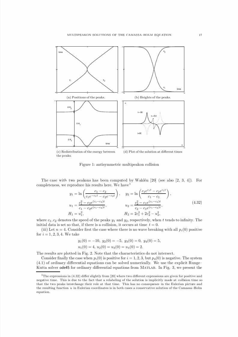
8/3/2019 Xavier Raynaud- On a Shallow Water Wave Equation
http://slidepdf.com/reader/full/xavier-raynaud-on-a-shallow-water-wave-equation 129/161
MULTIPEAKON SOLUTIONS OF THE CAMASSA–HOLM EQUATION 17
−5 0 5−5E
0
5E
y2
y1
time
(a) Positions of the peaks.
−5E 0 5E−E/2
0
E/2
u2
u1
time
(b) Heights of the peaks.
−5E 0 5E0
E^2
δ H0
δ H1
δ H2
time
(c) Redistribution of the energy betweenthe p eaks.
−20 0 20−E
0
E
t=−5E
t=−E/2
t=5E
u
x
(d) Plot of the solution at different times
Figure 1: antisymmetric multipeakon collision
The case with two peakons has been computed by Wahlen [20] (see also [2, 3, 4]). Forcompleteness, we reproduce his results here. We have1
y1 = ln
c1 − c2
c1e−c1t − c2e−c2t
, y2 = ln
c1ec1t − c2ec2t
c1 − c2
,
u1 =c2
1 − c2e(c1−c2)t
c1 − c2e(c1−c2)t, u2 =
c22 − c1e(c1−c2)t
c2 − c1e(c1−c2)t,
H 1 = u21, H 2 = 2c2
1 + 2c22 − u2
2,
(4.32)
where c1, c2 denotes the speed of the peaks y1 and y2, respectively, when t tends to infinity. Theinitial data is set so that, if there is a collision, it occurs at time t = 0.
(iii) Let n = 4. Consider first the case where there is no wave breaking with all pi(0) positive
for i = 1, 2, 3, 4. We takey1(0) = −10, y2(0) = −5, y3(0) = 0, y4(0) = 5,
u1(0) = 4, u2(0) = u3(0) = u4(0) = 2.
The results are plotted in Fig. 2. Note that the characteristics do not intersect.Consider finally the case when pi(0) is positive for i = 1, 2, 3, but p4(0) is negative. The system
(4.1) of ordinary differential equations can be solved numerically. We use the explicit Runge–Kutta solver ode45 for ordinary differential equations from Matlab. In Fig. 3, we present the
1The expressions in (4.32) differ slightly from [20] where two different expressions are given for positive andnegative time. This is due to the fact that a relabeling of the solution is implicitly made at collision time sothat the two peaks interchange their role at that time. This has no consequence in the Eulerian picture andthe resulting function u in Eulerian coordinates is in both cases a conservative solution of the Camassa–Holmequation.
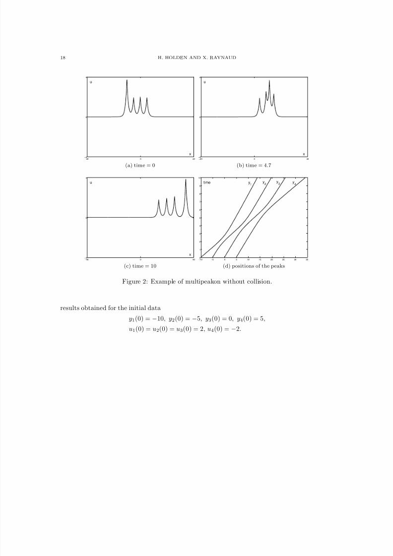
8/3/2019 Xavier Raynaud- On a Shallow Water Wave Equation
http://slidepdf.com/reader/full/xavier-raynaud-on-a-shallow-water-wave-equation 130/161
18 H. HOLDEN AND X. RAYNAUD
−40 0 40−4
0
4
u
x
(a) time = 0
−40 0 40−4
0
4
u
x
(b) time = 4.7
−40 0 40−4
0
4
u
x
(c) time = 10
−10 −5 0 5 10 15 20 25 30 350
1
2
3
4
5
6
7
8
9
10
time y1
y2
y3
y4
(d) positions of the peaks
Figure 2: Example of multipeakon without collision.
results obtained for the initial data
y1(0) = −10, y2(0) = −5, y3(0) = 0, y4(0) = 5,
u1(0) = u2(0) = u3(0) = 2, u4(0) = −2.
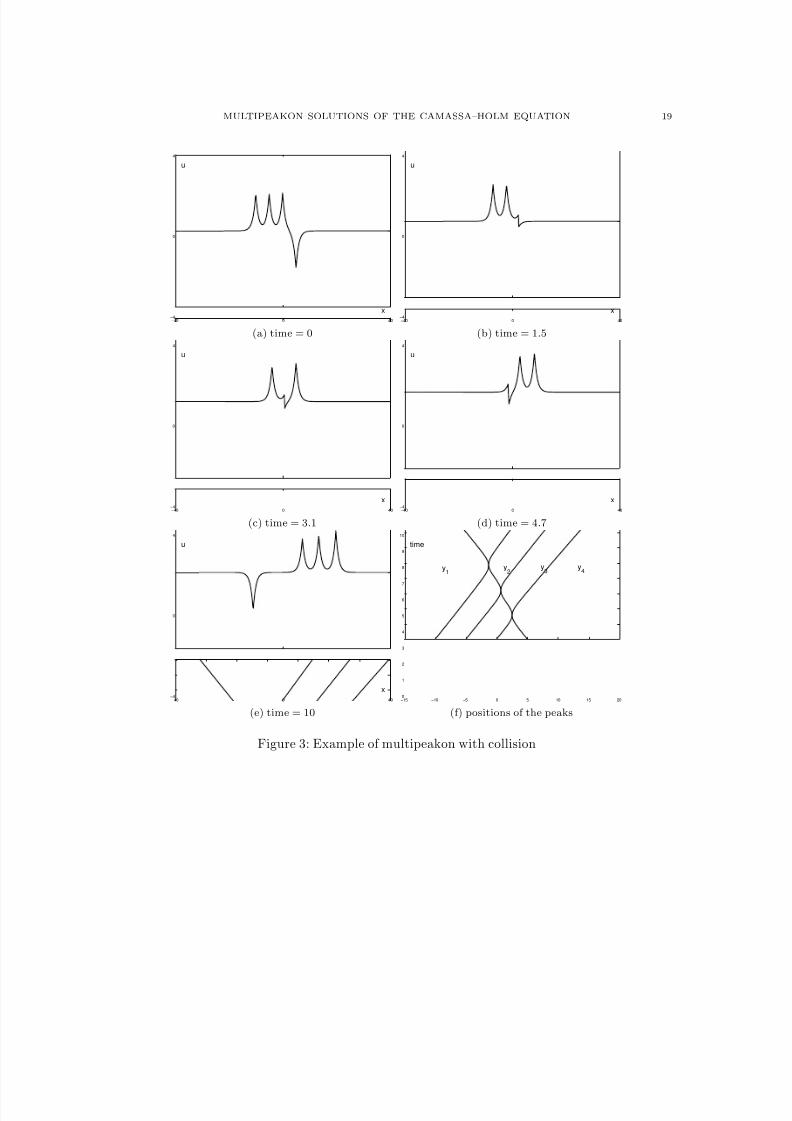
8/3/2019 Xavier Raynaud- On a Shallow Water Wave Equation
http://slidepdf.com/reader/full/xavier-raynaud-on-a-shallow-water-wave-equation 131/161
MULTIPEAKON SOLUTIONS OF THE CAMASSA–HOLM EQUATION 19
−40 0 40−4
0
4
u
x
(a) time = 0
−40 0 40−4
0
4
u
x
(b) time = 1.5
−40 0 40−4
0
4
u
x
(c) time = 3.1
−40 0 40−4
0
4
u
x
(d) time = 4.7
−40 0 40−4
0
4
u
x
(e) time = 10
−15 −10 −5 0 5 10 15 200
1
2
3
4
5
6
7
8
9
10
time
y1
y2
y3
y4
(f) positions of the peaks
Figure 3: Example of multipeakon with collision
8/3/2019 Xavier Raynaud- On a Shallow Water Wave Equation
http://slidepdf.com/reader/full/xavier-raynaud-on-a-shallow-water-wave-equation 132/161
20 H. HOLDEN AND X. RAYNAUD
Acknowledgments. The authors gratefully acknowledge the hospitality of the Mittag-LefflerInstitute, Sweden, creating a great working environment for research, during the Fall of 2005.This work has been supported in part by the Research Council of Norway.
References
[1] V. I. Arnold and B. A. Khesin. Topological Methods in Hydrodynamics. Springer-Verlag, New York, 1998.[2] R. Beals, D. Sattinger, and J. Szmigielski. Multi-peakons and a theorem of Stieltjes. Inverse Problems 15:L1–
L4, 1999.[3] R. Beals, D. Sattinger, and J. Szmigielski. Multipeakons and the classical moment problem. Adv. Math.
154:229–257, 2000.[4] R. Beals, D. Sattinger, and J. Szmigielski. Peakon-antipeakon interaction. J. Nonlinear Math. Phys. 8:23–27,
2001.[5] A. Bressan and A. Constantin. Global conservative solutions of the Camassa–Holm equation. Preprint , 2005,
submitted.[6] A. Bressan and M. Fonte. An optimal transportation metric for solutions of the Camassa–Holm equation.
Methods Appl. Anal., to appear.[7] R. Camassa. Characteristics and the initial value problem of a completely integrable shallow water equation.
Discrete Contin. Dyn. Syst. Ser. B , 3(1):115–139, 2003.[8] R. Camassa and D. D. Holm. An integrable shallow water equation with peaked solitons. Phys. Rev. Lett.,
71(11):1661–1664, 1993.[9] R. Camassa, D. D. Holm, and J. Hyman. A new integrable shallow water equation. Adv. Appl. Mech., 31:1–33,
1994.[10] R. Camassa, J. Huang, and L. Lee. Integral and integrable algorithms for a nonlinear shallow-water wave
equation. Preprint , 2004, submitted.[11] R. Camassa, J. Huang, and L. Lee. On a completely integrable numerical scheme for a nonlinear shallow-water
equation. Preprint , 2004, submitted.[12] G. M. Coclite, and H. Holden, and K. H, Karlsen. Well-posedness for a parabolic-elliptic system. Discrete
Cont. Dynam. Systems 13:659–682, 2005.[13] G. M. Coclite, and H. Holden, and K. H, Karlsen. Global weak solutions to a generalized hyperelastic-rod
wave equation. SIAM J. Math. Anal., 37:1044–1069, 2005.[14] A. Constantin and B. Kolev. On the geometric approach to the motion of inertial mechanical systems. J.
Phys. A, 35(32):R51–R79, 2002.
[15] M. Fonte. Conservative solution of the Camassa Holm equation on the real line. arXiv:math.AP/0511549 , 3,2005.[16] H. Holden and X. Raynaud. Convergence of a finite difference scheme for the Camassa–Holm equation. SIAM
J. Numer. Anal. 2006, to appear. paper I in this thesis.[17] H. Holden and X. Raynaud. A convergent numerical scheme for the Camassa–Holm equation based on
multipeakons. Discrete Contin. Dyn. Syst., 14(3):505–523, 2006. paper II in this thesis.[18] H. Holden and X. Raynaud. Global conservative solutions of the Camassa–Holm equation — a Lagrangian
point of view. Preprint , 2006, submitted. paper IV in this thesis.[19] R. S. Johnson. Camassa–Holm, Korteweg–de Vries and related models for water waves. J. Fluid Mech.,
455:63–82, 2002.[20] E. Wahlen. On the peakon-antipeakon interaction. Dyn. Contin. Discrete Impuls. Syst. Ser. A Math. Anal.,
2006, to appear.

8/3/2019 Xavier Raynaud- On a Shallow Water Wave Equation
http://slidepdf.com/reader/full/xavier-raynaud-on-a-shallow-water-wave-equation 133/161
8/3/2019 Xavier Raynaud- On a Shallow Water Wave Equation
http://slidepdf.com/reader/full/xavier-raynaud-on-a-shallow-water-wave-equation 134/161
Paper VI
Global conservative solutionsof the generalized hyperelastic-rod wave equation.
H. Holden and X. RaynaudSubmitted for publication.

8/3/2019 Xavier Raynaud- On a Shallow Water Wave Equation
http://slidepdf.com/reader/full/xavier-raynaud-on-a-shallow-water-wave-equation 135/161
8/3/2019 Xavier Raynaud- On a Shallow Water Wave Equation
http://slidepdf.com/reader/full/xavier-raynaud-on-a-shallow-water-wave-equation 136/161
GLOBAL CONSERVATIVE SOLUTIONS OF THE GENERALIZEDHYPERELASTIC-ROD WAVE EQUATION
HELGE HOLDEN AND XAVIER RAYNAUD
Abstract. We prove existence of global and conservative solutions of the Cauchy problem forthe nonlinear partial differential equation ut−uxxt+f (u)x−f (u)xxx+(g(u)+ 1
2f (u)(ux)2)x =
0 where f is strictly convex or concave and g is locally uniformly Lipschitz. This includes theCamassa–Holm equation (f (u) = u2/2 and g(u) = κu+u2) as well as the hyperelastic-rod waveequation (f (u) = γu2/2 and g(u) = (3−γ )u2/2) as special cases. It is shown that the problemis well-posed for initial data in H 1(R) if one includes a Radon measure that corresponds tothe energy of the system with the initial data. The solution is energy preserving. Stabilityis proved both with respect to initial data and the functions f and g. The proof uses an
equivalent reformulation of the equation in terms of Lagrangian coordinates.
1. Introduction
We solve the Cauchy problem on the line for the equation
ut − uxxt + f (u)x − f (u)xxx + (g(u) +1
2f (u)(ux)2)x = 0 (1.1)
for strictly convex or concave functions f and locally uniformly Lipschitz functions g with initialdata in H 1(R). This equation includes the Camassa–Holm equation [4], the hyperelastic-rodwave equation [11] and its generalization [6, 7] as special cases.
For f (u) =u2
2 and g(u) = κu + u2
, we obtain the Camassa–Holm equation:ut − uxxt + κux + 3uux − 2uxuxx − uuxxx = 0, u|t=0 = u, (1.2)
which has been extensively studied the last decade [4, 5]. It was first introduced as a modeldescribing propagation of unidirectional gravitational waves in a shallow water approximation,with u representing the fluid velocity, see [18]. The Camassa–Holm equation has a bi-Hamiltonianstructure, it is completely integrable, and it has infinitely many conserved quantities.
For f (u) = γu2
2and g(u) = 3−γ
2u2, we obtain the hyperelastic-rod wave equation:
ut − utxx + 3uux − γ (2uxuxx + uuxxx) = 0,
which was introduced by Dai [11, 10, 12] in 1998. It describes far-field, finite length, finite am-plitude radial deformation waves in cylindrical compressible hyperelastic rods, and u representsthe radial stretch relative to a pre-stressed state.
Furthermore, for f (u) = γu22 we find the generalized hyperelastic-rod equation
ut − uxxt +1
2g(u)x − γ (2uxuxx + uuxxx) = 0, (1.3)
which was recently studied by Coclite, Holden, and Karlsen [6, 7], extending earlier results for theCamassa–Holm equation by Xin and Zhang, see [20]. They analyzed the initial value problem forthis equation, using an approach based on a certain viscous regularization. By carefully studyingthe behavior of the limit of vanishing viscosity they derived the existence of a solution of (1.3).
2000 Mathematics Subject Classification. Primary: 65M06, 65M12; Secondary: 35B10, 35Q53.Key words and phrases. Generalized hyperelastic-rod wave equation, Camassa–Holm equation, conservative
solutions.Supported in part by the Research Council of Norway and the Mittag-Leffler Institute, Sweden.
1
8/3/2019 Xavier Raynaud- On a Shallow Water Wave Equation
http://slidepdf.com/reader/full/xavier-raynaud-on-a-shallow-water-wave-equation 137/161
2 H. HOLDEN AND X. RAYNAUD
This solution could be called a diffusive solution, and will be distinct from the solutions studiedhere. We will discuss this in more detail below.
We will not try to cover the extensive body of results regarding various aspects of the Camassa–
Holm equation. Suffice it here to note that in the case with κ = 0 the solution may experiencewave breaking in finite time in the sense that the function remains bounded while the spatialderivative becomes unbounded with finite H 1-norm. Various mechanisms and conditions areknown as to when and if wave breaking occurs. Specifically we mention that Constantin, Escher,and Molinet [8, 9] showed the following result: If the initial data u|t=0 = u ∈ H 1(R) andm := u − u is a positive Radon measure, then equation (1.2) with κ = 0 has a unique globalweak solution u ∈ C ([0, T ], H 1(R)), for any T positive, with initial data u. However, any solutionwith odd initial data u in H 3(R) such that ux(0) < 0 blows up in a finite time.
The problem of continuation of the solution beyond wave breaking is intricate. It can beillustrated in the context of a peakon–antipeakon solution. The one peakon is given by u(t, x) =c exp(− |x − ct|). If c is positive, the solution is called a peakon, and with c negative it is called anantipeakon. One can construct solutions that consist of finitely many peakons and antipeakons.Peakons move to the right, antipeakons to the left. If initial data are given appropriately, onecan have a peakon colliding with an antipeakon. In a particular symmetric case they exactlyannihilate each other at collision time t∗, thus u(t∗, x) = 0. This immediately raises the questionabout well-posedness of the equation and allows for several distinct ways to continue the solutionbeyond collision time. For an extensive discussion of this case, we refer to [17] and referencestherein. We here consider solutions, called conservative, that preserve the energy. In the example just mentioned this corresponds to the peakon and antipeakon passing through each other, andthe energy accumulating as a Dirac delta-function at the origin at the time of collision. Thus theproblem cannot be well-posed by considering the solution u only. Our approach for the generalequation (1.1) is based on the inclusion of the energy, in the form of a (non-negative Radon)measure, together with the function u as initial data. We have seen that singularities occur inthese variables. Therefore we transform to a different set of variables, which corresponds to aLagrangian formulation of the flow, where the singularities do not occur.
Let us comment on the approach in [6, 7]. The equation (1.3) is rewritten as
ut + γuux + P x = 0, P − P xx =1
2(g(u) − γu2) + γ (ux)2. (1.4)
By adding the term uxx to the first equation, it is first shown that the modified system hasa unique solution.1 Subsequently, it is proved that the vanishing viscosity limit → 0 exists.The limit is shown to be weak solution of (1.3). In particular, that means that u(t, · )H 1 ≤u(0, · )H 1 and that the solution satisfies an entropy condition ux(t, x) ≤ K + 2/(γt) for someconstant K . The solution described above with a peakon and an antipeakon “passing through”each other will not satisfy this entropy condition. Thus the solution concept is different in thetwo approaches.
Here we take a rather different approach. Based on recent techniques developed for theCamassa–Holm equation, see [1, 2, 15, 16], we prove that (1.1) possesses a global weak and
conservative solution. Furthermore, we show that the problem is well-posed. In particular weshow stability with respect to both perturbations in the initial data and the functions f and gin a suitable topology.
The present approach is based on the fact that the equation can be reformulated as a system of ordinary differential equations taking values in a Banach space. It turns out to be advantageousfirst to rewrite the equation as
ut + f (u)x + P x = 0, (1.5a)
P − P xx = g(u) +1
2f (u)u2
x (1.5b)
1In fact, it it is proved that a more general parabolic-elliptic system, allowing, e.g., for explicit spatial andtemporal dependence in the various functions, has a solution.
8/3/2019 Xavier Raynaud- On a Shallow Water Wave Equation
http://slidepdf.com/reader/full/xavier-raynaud-on-a-shallow-water-wave-equation 138/161
CONSERVATIVE SOLUTIONS FOR A HYPERELASTIC ROD 3
where we assume2 f ∈ W 3,∞loc (R), f (u) = 0, u ∈ R,
g
∈W 1,∞loc (R), g(0) = 0.
(1.6)
We will use this assumption throughout the paper.Specifically, the characteristics are given by
yt(t, ξ) = f (u(t, y(t, ξ)).
Define subsequently
U (t, ξ) = u(t, y(t, ξ)),
H (t, ξ) =
y(t,ξ)
−∞
u2 + u2
x
dx,
where U and H correspond to the Lagrangian velocity and the Lagrangian cumulative energydistribution, respectively. It turns out that one can derive the following system of ordinarydifferential equations taking values in an appropriately chosen Banach space, viz.
yt = U,
U t = −Q,
H t = G(U ) − 2P U,
where the quantities G, Q, and P can be expressed in terms of the unknowns (y,U,H ). Short-term existence is derived by a contraction argument. Global existence as well as stability withrespect to both initial data and functions f and g, is obtained for a class of initial data thatincludes initial data u|t=0 = u in H 1(R), see Theorem 2.8. The transition of this result back toEulerian variables is complicated by several factors, one being the reduction of three Lagrangianvariables to two Eulerian variables. There is a certain redundancy in the Lagragian formulationwhich is identified, and we rather study equivalence classes that correspond to relabeling of thesame Eulerian flow. The main existence result is Theorem 2.9. It is shown that the flow is
well-posed on this space of equivalence classes in the Lagrangian variables, see Theorem 3.6. Abijection is constructed between Lagrangian and Eulerian variables, see Theorems 3.8–3.11. Onthe set D of Eulerian variables we introduce a metric that turns D into a complete metric space,see Theorem 3.12.
The main result, Theorem 3.13, states the following: There exists a continuous semigroup onD which to any initial data (u, µ) ∈ D associates the pair (u(t), µ(t)) ∈ D such that u(t) is aweak solution of (1.5) and the measure µ = µ(t) with µ(0) = µ, evolves according to the lineartransport equation µt + (uµ)x = (G(u) − 2P u)x where the functions G and P are explicitlygiven. Continuity with respect to all variables, including f and g, is proved. The total energyas measured by µ is preserved, i.e., µ(t)(R) = µ(R) for all t.
The abstract construction is illustrated on the one and two peakon solutions for the Camassa–Holm equation.
The paper is organized as follows. In Section 2 the equation is reformulated in terms of Lagrangian variables, and existence is first proved in Lagrangian variables before the results aretransformed back to the original Eulerian variables. Stability of the semigroup is provided inSection 3, and the construction is illustrated on concrete examples in Section 4.
2. Existence of solutions
2.1. Transport equation for the energy density and reformulation in terms of La-
grangian variables. In (1.5b), P can be written in explicit form:
P (t, x) =1
2
R
e−|x−z|
g ◦ u +1
2f ◦ uu2
x
(t, z) dz. (2.1)
2Without loss of generality we may and will assume that g(0) = 0. Otherwise, (1.5b) should be replaced by
P − P xx = g(u)− g(0) + 1
2f (u)u2x
8/3/2019 Xavier Raynaud- On a Shallow Water Wave Equation
http://slidepdf.com/reader/full/xavier-raynaud-on-a-shallow-water-wave-equation 139/161
4 H. HOLDEN AND X. RAYNAUD
We will derive a transport equation for the energy density u2 + u2x. Assuming that u is smooth,
we get, after differentiating (1.5a) with respect to x and using (1.5b), that
uxt +
1
2 f (u)u2
x + f (u)uxx + P − g(u) = 0. (2.2)Multiply (1.5a) by u, (2.2) by ux, add the two to find the following equation
(u2 + u2x)t + (f (u)(u2 + u2
x))x = −2(P u)x + (2g(u) + f (u)u2)ux. (2.3)
Define G(v) as
G(v) =
v0
(2g(z) + f (z)z2) dz, (2.4)
then (2.3) can be rewritten as
(u2 + u2x)t + (f (u)(u2 + u2
x))x = (G(u) − 2P u)x, (2.5)
which is transport equation for the energy density u2 + u2x.
Let us introduce the characteristics y(t, ξ) defined as the solutions of
yt(t, ξ) = f (u(t, y(t, ξ)) (2.6)
with y(0, ξ) given. Equation (2.5) gives us information about the evolution of the amount of energy contained between two characteristics. Indeed, given ξ1, ξ2 in R, let
H (t) =
y(t,ξ2)
y(t,ξ1)
u2 + u2
x
dx
be the energy contained between the two characteristic curves y(t, ξ1) and y(t, ξ2). Then, wehave
dH
dt=
yt(t, ξ)(u2 + u2x) ◦ y(t, ξ)
ξ2ξ1
+
y(t,ξ2)
y(t,ξ1)
(u2 + u2x)t dx. (2.7)
We use (2.5) and integrate by parts. The first term on the right-hand side of (2.7) cancelsbecause of (2.6) and we end up with
dH
dt= [(G(u) − 2P u) ◦ y]
ξ2ξ1
. (2.8)
We now derive a system equivalent to (1.5). The calculations here are formal and will be justifiedlater. Let y still denote the characteristics. We introduce two other variables, the Lagrangianvelocity U and cumulative energy distribution H defined by
U (t, ξ) = u(t, y(t, ξ)), (2.9)
H (t, ξ) =
y(t,ξ)
−∞
u2 + u2
x
dx, (2.10)
respectively. From the definition of the characteristics, it follows from (1.5a) that
U t(t, ξ) = ut(t, y) + yt(t, ξ)ux(t, y)
= (ut + f (u)ux) ◦ y(t, ξ)
= −P x◦y (t, ξ). (2.11)
This last term can be expressed uniquely in term of U , y, and H . Namely, we have
P x◦y (t, ξ) = −1
2
R
sgn(y(t, ξ) − z)e−|y(t,ξ)−z|(g ◦ u +1
2f ◦ u u2
x)(t, z) dz
and, after the change of variables z = y(t, η),
P x ◦ y(t, ξ) = −1
2
R
sgn(y(t, ξ) − y(t, η))e−|y(t,ξ)−y(t,η)|
× g ◦ u +1
2f ◦ uu2
x(t, y(t, η))yξ(t, η) dη.
8/3/2019 Xavier Raynaud- On a Shallow Water Wave Equation
http://slidepdf.com/reader/full/xavier-raynaud-on-a-shallow-water-wave-equation 140/161
CONSERVATIVE SOLUTIONS FOR A HYPERELASTIC ROD 5
Finally, since H ξ = (u2 + u2x)◦y yξ,
P x
◦y (ξ) =
−
1
2 R
sgn(y(ξ)
−y(η))e−|y(ξ)−y(η)|
×
g(U ) − 1
2f (U )U 2
yξ +
1
2f (U )H ξ
(η) dη (2.12)
where the t variable has been dropped to simplify the notation. Later we will prove that y is anincreasing function for any fixed time t. If, for the moment, we take this for granted, then P x◦yis equivalent to Q where
Q(t, ξ) = −1
2
R
sgn(ξ − η)exp− sgn(ξ − η)(y(ξ) − y(η))
×
g(U ) − 1
2f (U )U 2
yξ +
1
2f (U )H ξ
(η) dη, (2.13)
and, slightly abusing the notation, we write
P (t, ξ) = 12
R
exp− sgn(ξ − η)(y(ξ) − y(η))
×
g(U ) − 1
2f (U )U 2
yξ +
1
2f (U )H ξ
(η) dη. (2.14)
Thus P x◦y and P ◦y can be replaced by equivalent expressions given by (2.13) and (2.14) whichonly depend on our new variables U , H , and y. We introduce yet another variable, ζ (t, ξ), simplydefined as
ζ (t, ξ) = y(t, ξ) − ξ.
It will turn out that ζ ∈ L∞(R). We have now derived a new system of equations, formallyequivalent (1.5). Equations (2.11), (2.8) and (2.6) give us
ζ t = U,
U t = −Q,H t = G(U ) − 2P U.
(2.15)
Detailed analysis will reveal that the system (2.15) of ordinary differential equations for (ζ , U , H ): [0, T ] →E is well-posed, where E is a Banach space to be defined in the next section. We have
Qξ = −1
2f (U )H ξ +
P +
1
2f (U )U 2 − g(U )
yξ,
and P ξ = Qyξ. Hence, differentiating (2.15) yields
ζ ξt = f (U )U ξ (or yξt = f (U )U ξ),
U ξt =1
2f (U )H ξ −
P +
1
2f (U )U 2 − g(U )
yξ,
H ξt = −2Q U yξ + (2g(U ) − f (U )U 2
− 2P )U ξ.
(2.16)
The system (2.16) is semilinear with respect to the variables yξ, U ξ and H ξ.
2.2. Existence and uniqueness of solutions in Lagrangian variables. In this section, wefocus our attention on the system of equations (2.15) and prove, by a contraction argument, thatit admits a unique solution. Let V be the Banach space defined by
V = {f ∈ C b(R) | f ξ ∈ L2(R)}where C b(R) = C (R) ∩ L∞(R) and the norm of V is given by f V = f L∞(R) + f ξL2(R). Of
course H 1(R) ⊂ V but the converse is not true as V contains functions that do not vanish atinfinity. We will employ the Banach space E defined by
E = V
×H 1(R)
×V
8/3/2019 Xavier Raynaud- On a Shallow Water Wave Equation
http://slidepdf.com/reader/full/xavier-raynaud-on-a-shallow-water-wave-equation 141/161
6 H. HOLDEN AND X. RAYNAUD
to carry out the contraction map argument. For any X = (ζ , U , H ) ∈ E , the norm on E is givenby
X
E =
ζ
V +
U
H 1(R) +
H
V .
The following lemma gives the Lipschitz bounds we need on Q and P .
Lemma 2.1. For any X = (ζ , U , H ) in E , we define the maps Q and P as Q(X ) = Q and P (X ) = P where Q and P are given by (2.13) and (2.14), respectively. Then, P and Q areLipschitz maps on bounded sets from E to H 1(R). Moreover, we have
Qξ = −1
2f (U )H ξ +
P +
1
2f (U )U 2 − g(U )
(1 + ζ ξ), (2.17)
P ξ = Q(1 + ζ ξ). (2.18)
Proof. We rewrite Q as
Q(X )(ξ) =
−e−ζ(ξ)
2 R
χ
{η<ξ
}(η)e−(ξ−η)eζ(η)
×
g(U ) − 1
2f (U )U 2
(1 + ζ ξ) +
1
2f (U )H ξ
(η) dη
+eζ(ξ)
2
R
χ{η>ξ}(η)e(ξ−η)e−ζ(η)
×
g(U ) − 1
2f (U )U 2
(1 + ζ ξ) +
1
2f (U )H ξ
(η) dη, (2.19)
where χB denotes the indicator function of a given set B. We decompose Q into the sum Q1 +Q2
where Q1 and Q2 are the operators corresponding to the two terms on the right-hand side of (2.19). Let h(ξ) = χ{ξ>0}(ξ)e−ξ and A be the map defined by A : v → h v. Then, Q1 can berewritten as
Q1(X )(ξ) = −e−ζ(ξ)
2 A ◦ R(ζ , U , H )(ξ) (2.20)
where R is the operator from E to L2(R) given by
R(ζ , U , H )(ξ) = eζ(ξ)
(g(U ) − 1
2f (U )U 2)(1 + ζ ξ) +
1
2f (U )H ξ
(ξ). (2.21)
We claim that A is continuous from L2(R) into H 1(R). The Fourier transform of h can easilybe computed, and we obtain
h(η) =
R
h(ξ)e−2iπηξ dξ =1
1 + 2iπη. (2.22)
The H 1(R) norm can be expressed in term of the Fourier transform as follows, see, e.g., [14],
h vH 1(R) =
(1 + η2
)
1
2 h v
L2(R) .
Since h v = hv, we have
h vH 1(R) =(1 + η2)
12 hv
L2(R)
≤ C vL2(R) by (2.22)
= C vL2(R) by Plancherel equality
for some constant C . Hence, A : L2(R) → H 1(R) is continuous. We prove that R(ζ , U , H )belongs to L2(R) by using the assumption that g(0) = 0. Then, A ◦ R(ζ , U , H ) belongs to H 1.Let us prove that R : E → L2(R) is locally Lipschitz. For that purpose we will use the followingshort lemma.
8/3/2019 Xavier Raynaud- On a Shallow Water Wave Equation
http://slidepdf.com/reader/full/xavier-raynaud-on-a-shallow-water-wave-equation 142/161
CONSERVATIVE SOLUTIONS FOR A HYPERELASTIC ROD 7
Lemma 2.2. Let BM = {X ∈ E | X E ≤ M } be a bounded set of E .(i) If g1 is Lipschitz from BM to L∞(R) and g2 Lipschitz from BM to L2(R), then the product g1g2 is Lipschitz from BM to L2(R).
(ii) If g1, g2 are two Lipschitz maps from BM to L∞(R), then the product g1g2 is Lipschitz from BM to L∞(R).
Proof of Lemma 2.2. Let X and X be in BM , and assume that g1 and g2 satisfy the assumptionsof (i ). We denote by L1 and L2, the Lipschitz constants of g1 and g2, respectively. We haveg1(X )g2(X ) − g1(X )g2(X )
L2(R)
≤ g1(X ) − g1(X )L∞(R)
g2(X )L2(R) +g1(X )
L∞(R)
g2(X ) − g2(X )L2(R)
≤ 2L1L2M + L1 g2(0)L2(R) + L2 g1(0)L∞(R)
X − X E
and (i ) is proved. One proves (ii ) the same way.
Let us consider a bounded set BM = {X ∈ E | X E ≤ M } of E . For X = (ζ , U , H ) and
X = (ζ , U , H ) in BM , we have
U L
∞
(R
) ≤1
√2 U
H 1
(R
) ≤1
√2
M , because 1
√2
is the constant
of the Sobolev embedding from H 1(R) into L∞(R), and, similarly,U L∞(R)
≤ 1√2
M . Let
I M = [− 1√2
M, 1√2
M ] and
LM = f W 3,∞(I M) + gW 1,∞(I M) < ∞. (2.23)
Then g(U ) − g(U )L2(R)
≤ gW 1,∞(I M )
U − U L2(R)
≤ LM
U − U L2(R)
.
Hence, g1 : X → g(U ) is Lipschitz from BM to L2(R). For X, X in BM , we have ζ L∞(R) ≤ M
andζ L∞(R)
≤ M . The function x → ex is Lipschitz on {x ∈ R | |x| ≤ M }. Hence, g2 : X → eζ
is Lipschitz from BM to L∞(R). Thus, the first term in (2.21), g1(X )g2(X ) = eζg(U ), is, byLemma 2.2, Lipschitz from BM to L2(R). We look at the second term, that is, eζg(U )ζ ξ . ForX, X in BM , we haveg(U ) − g(U )
L∞(R)
≤ gW 1,∞(I M )
U − U L∞(R)
≤ 1√2
LM
U − U H 1(R)
.
Hence, X → g(U ) is Lipschitz from BM to L∞(R) and, by Lemma 2.2, as X → eζ is alsoLipschitz from BM to L∞(R), we have that the product X → eζg(U ) is Lipschitz from BM toL∞(R). After using again Lemma 2.2, since X → ζ ξ, being linear, is obviously Lipschitz fromBM to L2(R), we obtain, as claimed, that the second term in (2.21), eζg(U )ζ ξ, is Lipschitz fromBM to L2(R). We can handle the other terms in (2.21) similarly and prove that R is Lipschitzfrom BM to L2(R). Since A : L2(R) → H 1(R) is linear and continuous, A ◦ R is Lipschitz fromBM to H 1(R). Then, we use the following lemma whose proof is basically the same as the proof of Lemma 2.2.
Lemma 2.3. Let
R1 : BM
→V ,
R2 : BM
→H 1(R), and
R3 : BM
→V be three Lipschitz maps.
Then, the products X → R1(X )R2(X ) and X → R1(X )R3(X ) are also Lipschitz maps from BM
to H 1(R) and BM to V , respectively.
Since the map X → e−ζ is Lipschitz from BM to V , Q1 is the product of two Lipschitz maps,one from BM to H 1(R) and the other from BM to V , and therefore it is Lipschitz map from BM
to H 1(R). Similarly, one proves that Q2 and therefore Q are Lipschitz on BM . Furthermore, P is Lipschitz on BM . The formulas (2.17) and (2.18) are obtained by direct computation usingthe product rule, see [13, p. 129].
In the next theorem, by using a contraction argument, we prove the short-time existence of solutions to (2.15).
Theorem 2.4. Given X = (ζ , U , H ) in E , there exists a time T depending only on
X
E
such
that the system (2.15) admits a unique solution in C 1([0, T ], E ) with initial data X .
8/3/2019 Xavier Raynaud- On a Shallow Water Wave Equation
http://slidepdf.com/reader/full/xavier-raynaud-on-a-shallow-water-wave-equation 143/161
8 H. HOLDEN AND X. RAYNAUD
Proof. Solutions of (2.15) can be rewritten as
X (t) = X + t
0
F (X (τ )) dτ (2.24)
where F : E → E is given by F (X ) = (f (U ), −Q(X ), G(U ) − 2P (X )U ) where X = (ζ , U , H ).The integrals are defined as Riemann integrals of continuous functions on the Banach spaceE . Let BM and LM be defined as in the proof of Lemma 2.1, see (2.23). We claim thatX = (ζ , U , H ) → f (U ) and X = (ζ , U , H ) → G(U ) are Lipschitz from BM to V . Then, usingLemma 2.1, we can check that each component of F (X ) is a product of functions that satisfy oneof the assumptions of Lemma 2.3 and using this same lemma, we obtain that F (X ) is Lipchitzon BM . Thus, F is Lipschitz on any bounded set of E . Since E is a Banach space, we use thestandard contraction argument to show the existence of short-time solutions and the theoremis proved. For any X = (ζ , U , H ) and X = (ζ , U , H ) in BM , we have U L∞(R) ≤ 1√
2M and
U L∞(R)
≤ 1√2
M . Then,
f (U ) − f (U )
L∞(R) ≤ f W 1,∞(I M )
U − U
L∞(R) ≤
1
√2 LM
X − X E
and X → f (U ) is Lipschitz from BM into L∞(R). Since f is C 1 and U ∈ H 1(R), using [19,Appendix A.1], we obtain that f (U )ξ ∈ L2(R) and
f (U )ξ = f (U )U ξ .
As before, it is not hard to prove that X → f (U ) is Lipschitz from BM into L∞(R). It isclear that X → U ξ is Lipschitz from BM into L2(R). Hence, it follows from Lemma 2.2 thatX → f (U )U ξ is Lipschitz from BM into L2(R). Therefore, X → f (U ) is Lipschitz from BM
into V . Similarly, one proves that X → G(U ) is Lipschitz from BM into V and our previousclaim is proved.
We now turn to the proof of existence of global solutions of (2.15). We are interested in a
particular class of initial data that we are going to make precise later, see Definition 2.5. Inparticular, we will only consider initial data that belong to E ∩ W 1,∞(R)
3where
W 1,∞(R) = {f ∈ C b(R) | f ξ ∈ L∞(R)}.
Given (ζ , U , H ) ∈ E ∩ [W 1,∞(R)]3, we consider the short-time solution (ζ , U , H ) ∈ C ([0, T ], E ) of (2.15) given by Theorem 2.4. Using the fact that Q and P are Lipschitz on bounded sets (Lemma2.1) and, since X ∈ C ([0, T ], E ), we can prove that P and Q belongs to C ([0, T ], H 1(R)). Wenow consider U , P and Q as given function in C ([0, T ], H 1(R)). Then, for any fixed ξ ∈ R, wecan solve the system of ordinary differential equations
d
dtα(t, ξ) = f (U )β (t, ξ),
d
dt β (t, ξ) =
1
2 f (U )γ (t, ξ) +−
1
2 f (U )U 2
+ g(U ) − P
(1 + α)(t, ξ),d
dtγ (t, ξ) = −2(Q U )(1 + α)(t, ξ) + (2g(U ) + f (U )U 2 − 2P )β (t, ξ),
(2.25)
which is obtained by substituting ζ ξ , U ξ and H ξ in (2.16) by the unknowns α, β , and γ , re-spectively. Concerning the initial data, we set (α(0, ξ), β (0, ξ), γ (0, ξ)) = (ζ ξ , U ξ, H ξ) if
ζ ξ(ξ) +U ξ(ξ)
+H ξ(ξ)
< ∞ and (α(0, ξ), β (0, ξ), γ (0, ξ)) = (0, 0, 0) otherwise. In the same way as in[16, Lemma 2.4], see also Lemma 2.6 below, we can prove that solutions of (2.25) exist in [0 , T ]and that, for all time t ∈ [0, T ],
(α(t, ξ), β (t, ξ), γ (t, ξ)) = (ζ ξ(t, ξ), U ξ(t, ξ), H ξ(t, ξ))
for almost every ξ ∈ R. Thus, we can select a special representative for (ζ ξ , U ξ, H ξ) given by(α,β,γ ), which is defined for all ξ
∈R and which, for any given ξ, satisfies the ordinary differential
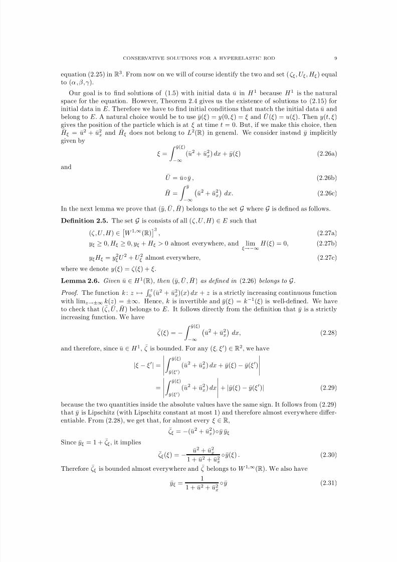
8/3/2019 Xavier Raynaud- On a Shallow Water Wave Equation
http://slidepdf.com/reader/full/xavier-raynaud-on-a-shallow-water-wave-equation 144/161
CONSERVATIVE SOLUTIONS FOR A HYPERELASTIC ROD 9
equation (2.25) in R3. From now on we will of course identify the two and set ( ζ ξ, U ξ, H ξ) equalto (α,β,γ ).
Our goal is to find solutions of (1.5) with initial data u in H 1 because H 1 is the natural
space for the equation. However, Theorem 2.4 gives us the existence of solutions to (2.15) forinitial data in E . Therefore we have to find initial conditions that match the initial data u andbelong to E . A natural choice would be to use y(ξ) = y(0, ξ) = ξ and U (ξ) = u(ξ). Then y(t, ξ)gives the position of the particle which is at ξ at time t = 0. But, if we make this choice, thenH ξ = u2 + u2
x and H ξ does not belong to L2(R) in general. We consider instead y implicitlygiven by
ξ =
y(ξ)
−∞(u2 + u2
x) dx + y(ξ) (2.26a)
and
U = u◦y , (2.26b)
H = y−∞ u2 + u2
x dx. (2.26c)
In the next lemma we prove that (y, U , H ) belongs to the set G where G is defined as follows.
Definition 2.5. The set G is consists of all (ζ , U , H ) ∈ E such that
(ζ , U , H ) ∈ W 1,∞(R)3
, (2.27a)
yξ ≥ 0, H ξ ≥ 0, yξ + H ξ > 0 almost everywhere, and limξ→−∞
H (ξ) = 0, (2.27b)
yξH ξ = y2ξU 2 + U 2ξ almost everywhere, (2.27c)
where we denote y(ξ) = ζ (ξ) + ξ.
Lemma 2.6. Given u ∈ H 1(R), then (y, U , H ) as defined in (2.26) belongs to G.
Proof. The function k : z → z0 (u
2
+ u2
x)(x) dx + z is a strictly increasing continuous functionwith limz→±∞ k(z) = ±∞. Hence, k is invertible and y(ξ) = k−1(ξ) is well-defined. We haveto check that (ζ , U , H ) belongs to E . It follows directly from the definition that y is a strictlyincreasing function. We have
ζ (ξ) = − y(ξ)
−∞
u2 + u2
x
dx, (2.28)
and therefore, since u ∈ H 1, ζ is bounded. For any (ξ, ξ) ∈ R2, we have
|ξ − ξ| =
y(ξ)
y(ξ)
(u2 + u2x) dx + y(ξ) − y(ξ)
=
y(ξ)
y(ξ)
(u2 + u2x) dx +
|y(ξ)
−y(ξ)
|(2.29)
because the two quantities inside the absolute values have the same sign. It follows from (2.29)that y is Lipschitz (with Lipschitz constant at most 1) and therefore almost everywhere differ-entiable. From (2.28), we get that, for almost every ξ ∈ R,
ζ ξ = −(u2 + u2x)◦y yξ
Since yξ = 1 + ζ ξ, it implies
ζ ξ(ξ) = − u2 + u2x
1 + u2 + u2x
◦y(ξ) . (2.30)
Therefore ζ ξ is bounded almost everywhere and ζ belongs to W 1,∞(R). We also have
yξ =1
1 + u2 + u2x
◦y (2.31)
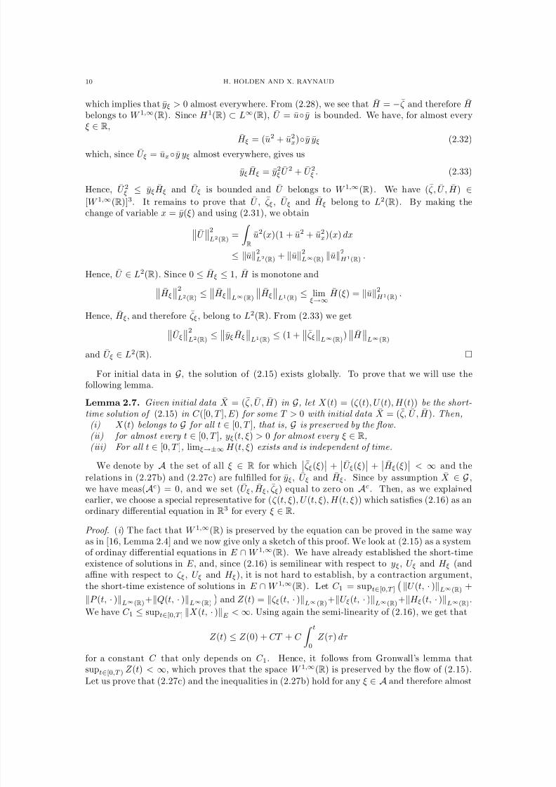
8/3/2019 Xavier Raynaud- On a Shallow Water Wave Equation
http://slidepdf.com/reader/full/xavier-raynaud-on-a-shallow-water-wave-equation 145/161
10 H. HOLDEN AND X. RAYNAUD
which implies that yξ > 0 almost everywhere. From (2.28), we see that H = −ζ and therefore H belongs to W 1,∞(R). Since H 1(R) ⊂ L∞(R), U = u◦ y is bounded. We have, for almost everyξ
∈R,
H ξ = (u2 + u2x)◦y yξ (2.32)
which, since U ξ = ux◦y yξ almost everywhere, gives us
yξH ξ = y2ξ U 2 + U 2ξ . (2.33)
Hence, U 2ξ ≤ yξH ξ and U ξ is bounded and U belongs to W 1,∞(R). We have (ζ , U , H ) ∈[W 1,∞(R)]3. It remains to prove that U , ζ ξ , U ξ and H ξ belong to L2(R). By making thechange of variable x = y(ξ) and using (2.31), we obtainU
2
L2(R)=
R
u2(x)(1 + u2 + u2x)(x) dx
≤ u2L2(R) + u2
L∞(R) u2H 1(R) .
Hence, U ∈ L2
(R). Since 0 ≤ H ξ ≤ 1, H is monotone andH ξ2
L2(R)≤ H ξ
L∞(R)
H ξL1(R)
≤ limξ→∞
H (ξ) = u2H 1(R) .
Hence, H ξ, and therefore ζ ξ , belong to L2(R). From (2.33) we getU ξ2
L2(R)≤ yξH ξ
L1(R)
≤ (1 +ζ ξL∞(R)
)H
L∞(R)
and U ξ ∈ L2(R).
For initial data in G, the solution of (2.15) exists globally. To prove that we will use thefollowing lemma.
Lemma 2.7. Given initial data X = (ζ , U , H ) in
G, let X (t) = (ζ (t), U (t), H (t)) be the short-
time solution of (2.15) in C ([0, T ], E ) for some T > 0 with initial data X = (ζ, U , H ). Then,(i) X (t) belongs to G for all t ∈ [0, T ], that is, G is preserved by the flow.(ii) for almost every t ∈ [0, T ], yξ(t, ξ) > 0 for almost every ξ ∈ R,(iii) For all t ∈ [0, T ], limξ→±∞ H (t, ξ) exists and is independent of time.
We denote by A the set of all ξ ∈ R for whichζ ξ(ξ)
+U ξ(ξ)
+H ξ(ξ)
< ∞ and the
relations in (2.27b) and (2.27c) are fulfilled for yξ, U ξ and H ξ. Since by assumption X ∈ G ,we have meas(Ac) = 0, and we set (U ξ , H ξ, ζ ξ) equal to zero on Ac. Then, as we explainedearlier, we choose a special representative for (ζ (t, ξ), U (t, ξ), H (t, ξ)) which satisfies (2.16) as anordinary differential equation in R3 for every ξ ∈ R.
Proof. (i ) The fact that W 1,∞(R) is preserved by the equation can be proved in the same wayas in [16, Lemma 2.4] and we now give only a sketch of this proof. We look at (2.15) as a system
of ordinay differential equations in E ∩ W 1,∞(R). We have already established the short-timeexistence of solutions in E , and, since (2.16) is semilinear with respect to yξ, U ξ and H ξ (andaffine with respect to ζ ξ, U ξ and H ξ), it is not hard to establish, by a contraction argument,the short-time existence of solutions in E ∩ W 1,∞(R). Let C 1 = supt∈[0,T ]
U (t, · )L∞(R) +
P (t, · )L∞(R)+Q(t, · )L∞(R)
and Z (t) = ζ ξ(t, · )L∞(R)+U ξ(t, · )L∞(R)+H ξ(t, · )L∞(R).
We have C 1 ≤ supt∈[0,T ] X (t, · )E < ∞. Using again the semi-linearity of (2.16), we get that
Z (t) ≤ Z (0) + CT + C
t0
Z (τ ) dτ
for a constant C that only depends on C 1. Hence, it follows from Gronwall’s lemma thatsupt∈[0,T ) Z (t) < ∞, which proves that the space W 1,∞(R) is preserved by the flow of (2.15).
Let us prove that (2.27c) and the inequalities in (2.27b) hold for any ξ
∈ Aand therefore almost
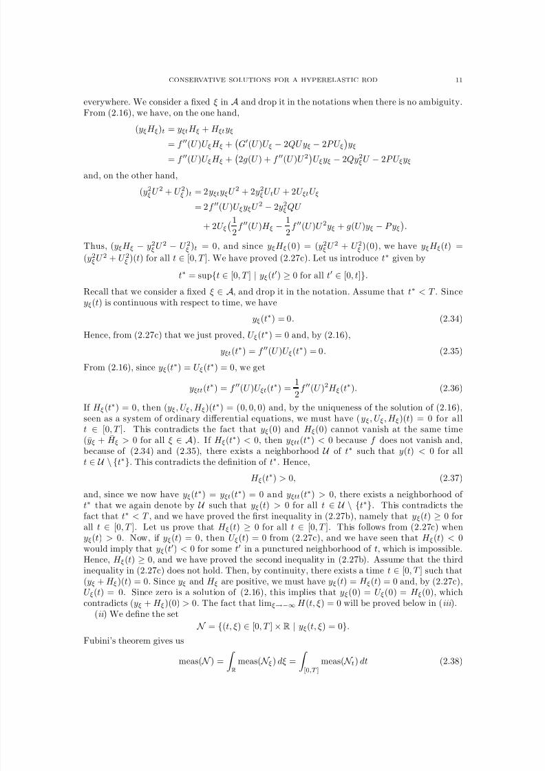
8/3/2019 Xavier Raynaud- On a Shallow Water Wave Equation
http://slidepdf.com/reader/full/xavier-raynaud-on-a-shallow-water-wave-equation 146/161
CONSERVATIVE SOLUTIONS FOR A HYPERELASTIC ROD 11
everywhere. We consider a fixed ξ in A and drop it in the notations when there is no ambiguity.From (2.16), we have, on the one hand,
(yξH ξ)t = yξtH ξ + H ξtyξ
= f (U )U ξH ξ +
G(U )U ξ − 2QU yξ − 2P U ξ
yξ
= f (U )U ξH ξ +
2g(U ) + f (U )U 2
U ξyξ − 2Qy2ξU − 2P U ξyξ
and, on the other hand,
(y2ξU 2 + U 2ξ )t = 2yξtyξU 2 + 2y2
ξU tU + 2U ξtU ξ
= 2f (U )U ξyξU 2 − 2y2ξQU
+ 2U ξ1
2f (U )H ξ − 1
2f (U )U 2yξ + g(U )yξ − P yξ
.
Thus, (yξH ξ − y2ξU 2 − U 2ξ )t = 0, and since yξH ξ(0) = (y2
ξU 2 + U 2ξ )(0), we have yξH ξ(t) =
(y2ξU 2 + U 2ξ )(t) for all t ∈ [0, T ]. We have proved (2.27c). Let us introduce t∗ given by
t∗ = sup{t ∈ [0, T ] | yξ(t) ≥ 0 for all t ∈ [0, t]}.
Recall that we consider a fixed ξ ∈ A, and drop it in the notation. Assume that t∗ < T . Sinceyξ(t) is continuous with respect to time, we have
yξ(t∗) = 0. (2.34)
Hence, from (2.27c) that we just proved, U ξ(t∗) = 0 and, by (2.16),
yξt(t∗) = f (U )U ξ(t∗) = 0. (2.35)
From (2.16), since yξ(t∗) = U ξ(t∗) = 0, we get
yξtt(t∗) = f (U )U ξt(t∗) =1
2f (U )2H ξ(t∗). (2.36)
If H ξ(t∗) = 0, then (yξ, U ξ, H ξ)(t∗) = (0, 0, 0) and, by the uniqueness of the solution of (2.16),seen as a system of ordinary differential equations, we must have ( yξ, U ξ, H ξ)(t) = 0 for allt ∈ [0, T ]. This contradicts the fact that yξ(0) and H ξ(0) cannot vanish at the same time(yξ + H ξ > 0 for all ξ ∈ A). If H ξ(t∗) < 0, then yξtt(t∗) < 0 because f does not vanish and,because of (2.34) and (2.35), there exists a neighborhood U of t∗ such that y(t) < 0 for allt ∈ U \ {t∗}. This contradicts the definition of t∗. Hence,
H ξ(t∗) > 0, (2.37)
and, since we now have yξ(t∗) = yξt(t∗) = 0 and yξtt(t∗) > 0, there exists a neighborhood of t∗ that we again denote by U such that yξ(t) > 0 for all t ∈ U \ {t∗}. This contradicts thefact that t∗ < T , and we have proved the first inequality in (2.27b), namely that yξ(t) ≥ 0 forall t ∈ [0, T ]. Let us prove that H ξ(t) ≥ 0 for all t ∈ [0, T ]. This follows from (2.27c) when
yξ(t) > 0. Now, if yξ(t) = 0, then U ξ(t) = 0 from (2.27c), and we have seen that H ξ(t) < 0would imply that yξ(t) < 0 for some t in a punctured neighborhood of t, which is impossible.Hence, H ξ(t) ≥ 0, and we have proved the second inequality in (2.27b). Assume that the thirdinequality in (2.27c) does not hold. Then, by continuity, there exists a time t ∈ [0, T ] such that(yξ + H ξ)(t) = 0. Since yξ and H ξ are positive, we must have yξ(t) = H ξ(t) = 0 and, by (2.27c),U ξ(t) = 0. Since zero is a solution of (2.16), this implies that yξ(0) = U ξ(0) = H ξ(0), whichcontradicts (yξ + H ξ)(0) > 0. The fact that limξ→−∞ H (t, ξ) = 0 will be proved below in (iii ).
(ii ) We define the set
N = {(t, ξ) ∈ [0, T ] ×R | yξ(t, ξ) = 0}.
Fubini’s theorem gives us
meas( N ) = R meas( N ξ) dξ = [0,T ]
meas( N t) dt (2.38)
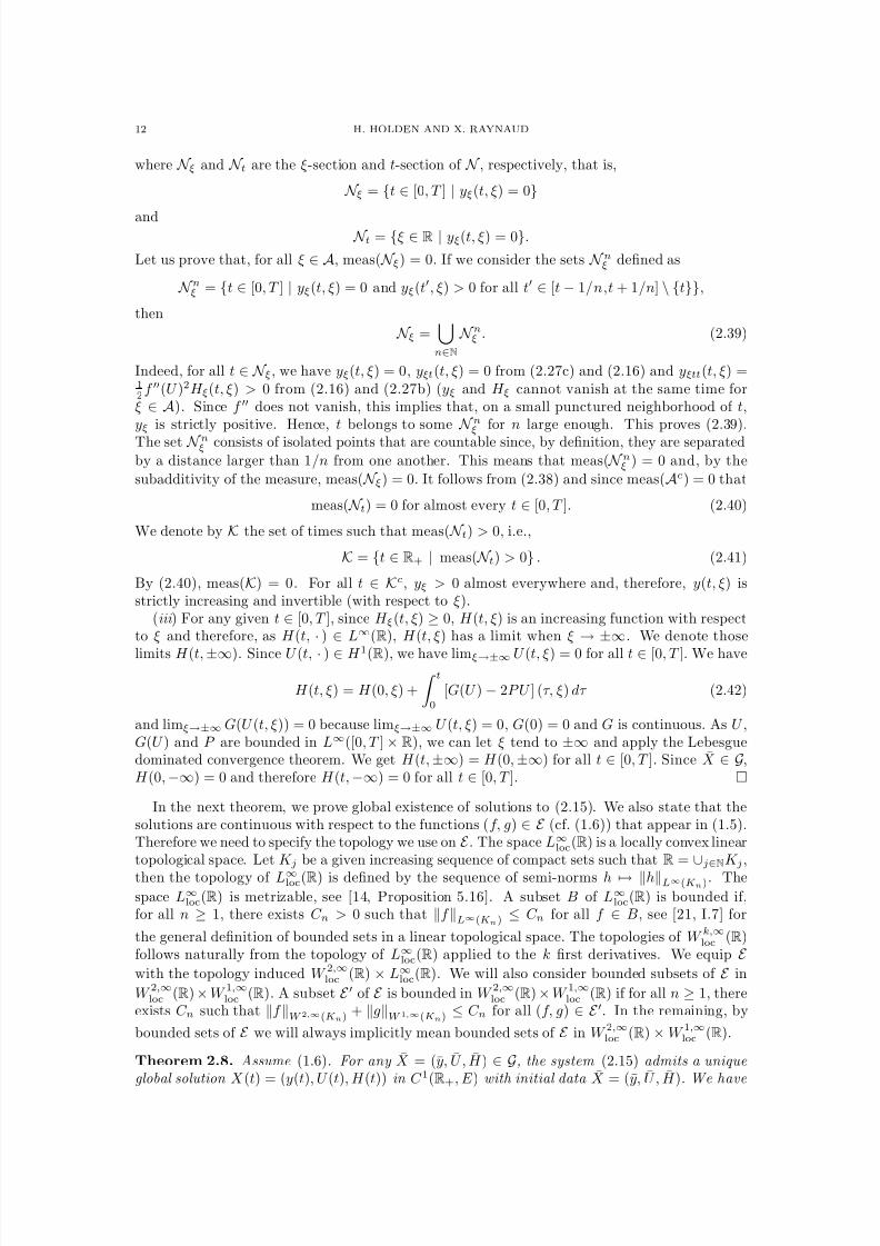
8/3/2019 Xavier Raynaud- On a Shallow Water Wave Equation
http://slidepdf.com/reader/full/xavier-raynaud-on-a-shallow-water-wave-equation 147/161
12 H. HOLDEN AND X. RAYNAUD
where N ξ and N t are the ξ-section and t-section of N , respectively, that is,
N ξ = {t ∈ [0, T ] | yξ(t, ξ) = 0}
and N t = {ξ ∈ R | yξ(t, ξ) = 0}.
Let us prove that, for all ξ ∈ A, meas( N ξ) = 0. If we consider the sets N nξ defined as
N nξ = {t ∈ [0, T ] | yξ(t, ξ) = 0 and yξ(t, ξ) > 0 for all t ∈ [t − 1/n,t + 1/n] \ {t}},
then
N ξ =n∈N
N nξ . (2.39)
Indeed, for all t ∈ N ξ, we have yξ(t, ξ) = 0, yξt(t, ξ) = 0 from (2.27c) and (2.16) and yξtt(t, ξ) =12
f (U )2H ξ(t, ξ) > 0 from (2.16) and (2.27b) (yξ and H ξ cannot vanish at the same time forξ ∈ A). Since f does not vanish, this implies that, on a small punctured neighborhood of t,yξ is strictly positive. Hence, t belongs to some
N nξ for n large enough. This proves (2.39).
The set N nξ consists of isolated points that are countable since, by definition, they are separatedby a distance larger than 1/n from one another. This means that meas( N nξ ) = 0 and, by the
subadditivity of the measure, meas( N ξ) = 0. It follows from (2.38) and since meas(Ac) = 0 that
meas( N t) = 0 for almost every t ∈ [0, T ]. (2.40)
We denote by K the set of times such that meas( N t) > 0, i.e.,
K = {t ∈ R+ | meas( N t) > 0} . (2.41)
By (2.40), meas(K) = 0. For all t ∈ Kc, yξ > 0 almost everywhere and, therefore, y(t, ξ) isstrictly increasing and invertible (with respect to ξ).
(iii ) For any given t ∈ [0, T ], since H ξ(t, ξ) ≥ 0, H (t, ξ) is an increasing function with respectto ξ and therefore, as H (t, · ) ∈ L∞(R), H (t, ξ) has a limit when ξ → ±∞. We denote those
limits H (t, ±∞). Since U (t, · ) ∈ H 1(R), we have limξ→±∞ U (t, ξ) = 0 for all t ∈ [0, T ]. We have
H (t, ξ) = H (0, ξ) +
t0
[G(U ) − 2P U ] (τ, ξ) dτ (2.42)
and limξ→±∞ G(U (t, ξ)) = 0 because limξ→±∞ U (t, ξ) = 0, G(0) = 0 and G is continuous. As U ,G(U ) and P are bounded in L∞([0, T ] × R), we can let ξ tend to ±∞ and apply the Lebesguedominated convergence theorem. We get H (t, ±∞) = H (0, ±∞) for all t ∈ [0, T ]. Since X ∈ G,H (0, −∞) = 0 and therefore H (t, −∞) = 0 for all t ∈ [0, T ].
In the next theorem, we prove global existence of solutions to (2.15). We also state that thesolutions are continuous with respect to the functions (f, g) ∈ E (cf. (1.6)) that appear in (1.5).Therefore we need to specify the topology we use on E . The space L∞
loc(R) is a locally convex lineartopological space. Let K j be a given increasing sequence of compact sets such that R =
∪j
∈NK j,
then the topology of L∞loc(R) is defined by the sequence of semi-norms h → hL∞(Kn). Thespace L∞loc(R) is metrizable, see [14, Proposition 5.16]. A subset B of L∞
loc(R) is bounded if,for all n ≥ 1, there exists C n > 0 such that f L∞(Kn) ≤ C n for all f ∈ B, see [21, I.7] for
the general definition of bounded sets in a linear topological space. The topologies of W k,∞loc (R)follows naturally from the topology of L∞
loc(R) applied to the k first derivatives. We equip E with the topology induced W 2,∞loc (R) × L∞loc(R). We will also consider bounded subsets of E in
W 2,∞loc (R) × W 1,∞loc (R). A subset E of E is bounded in W 2,∞loc (R) × W 1,∞loc (R) if for all n ≥ 1, thereexists C n such that f W 2,∞(Kn) + gW 1,∞(Kn) ≤ C n for all (f, g) ∈ E . In the remaining, by
bounded sets of E we will always implicitly mean bounded sets of E in W 2,∞loc (R) × W 1,∞loc (R).
Theorem 2.8. Assume (1.6). For any X = (y, U , H ) ∈ G, the system (2.15) admits a uniqueglobal solution X (t) = (y(t), U (t), H (t)) in C 1(R+, E ) with initial data X = (y, U , H ). We have
8/3/2019 Xavier Raynaud- On a Shallow Water Wave Equation
http://slidepdf.com/reader/full/xavier-raynaud-on-a-shallow-water-wave-equation 148/161
CONSERVATIVE SOLUTIONS FOR A HYPERELASTIC ROD 13
X (t) ∈ G for all times. If we equip G with the topology induced by the E -norm, then the mapS : G × E ×R+ → G defined as
S t(X , f , g) = X (t)
is a semigroup which is continuous with respect to all variables, on any bounded set of E .Proof. The solution has a finite time of existence T only if X (t, · )E blows up when t tendsto T because, otherwise, by Theorem 2.4, the solution can be extended by a small time intervalbeyond T . Thus, We want to prove that
supt∈[0,T )
X (t, · )E < ∞.
Since X (t) ∈ G, H ξ ≥ 0, from (2.27b), and H (t, ξ) is an increasing function in ξ for all t and,from Lemma 2.7, we have limξ→∞ H (t, ξ) = limξ→∞ H (0, ξ). Hence, supt∈[0,T ) H (t, · )L∞(R) =
H
L∞(R)and therefore supt∈[0,T ) H (t, · )L∞(R) is finite. To simplify the notation we suppress
the dependence in t for the moment and denote h =
H L∞(R). We have
U 2(ξ) = 2
ξ−∞
U (η)U ξ(η) dη = 2
{η≤ξ|yξ(η)>0}
U (η)U ξ(η) dη (2.43)
since, from (2.27c), U ξ(η) = 0 when yξ(η) = 0. For almost every ξ such that yξ(ξ) > 0, we have
|U (ξ)U ξ(ξ)| =
√yξU (ξ)U ξ(ξ)
yξ(ξ)
≤ 1
2
U (ξ)2yξ(ξ) +
U 2ξ (ξ)
yξ(ξ)
=
1
2H ξ(ξ),
from (2.27c). Inserting this inequality in (2.43), we obtain U 2(ξ) ≤ H (ξ) and we have
U (t, ξ)
∈I := [
−
√h,
√h] (2.44)
for all t ∈ [0, T ) and ξ ∈ R. Hence, supt∈[0,T ) U (t, · )L∞(R) < ∞. The property (2.44) is
important as it says that the L∞(R)-norm of U is bounded by a constant which does not dependon time. We set
κ = f W 2,∞(I ) + gW 1,∞(I ) .
By using (2.44), we obtain
f (U )L∞(R) ≤ f L∞(I ) ≤ κ. (2.45)
Hence, from the governing equation (2.15), it follows that
|ζ (t, ξ)| ≤ |ζ (0, ξ)| + κT,
and supt∈[0,T ) ζ (t, · )L∞(R) is finite. Next we prove that supt∈[0,T ) Q(t, · )L∞(R) is finite. Wedecompose Q into a sum of two integrals that we denote Qa and Qb, respectively,
Q(t, ξ) = −1
2
R
sgn(ξ − η)e−|y(ξ)−y(η)|yξ(η)
g(U ) − 1
2f (U )U 2
dη
− 1
4
R
sgn(ξ − η)e−|y(ξ)−y(η)|f (U )H ξ dη
:= Qa + Qb.
Since yξ ≥ 0, we have
|Qa(t, ξ)| ≤ C 1 R e−|y(ξ)−y(η)|yξ(η) dη = C 1 R e−|y(ξ)−x| dx = 2C 1
8/3/2019 Xavier Raynaud- On a Shallow Water Wave Equation
http://slidepdf.com/reader/full/xavier-raynaud-on-a-shallow-water-wave-equation 149/161
14 H. HOLDEN AND X. RAYNAUD
where the constant C 1 depends only on κ and h. Since H ξ ≥ 0, we have
|Qb(t, ξ)| ≤ κ
4 R e−|y(ξ)−y(η)|H ξ(η) dη
=κ
4
R
sgn(ξ − η)e−|y(ξ)−y(η)|H (η)yξ(η) dη (after integrating by parts)
≤ κh
4
R
e−|y(ξ)−y(η)|yξ(η) dη (as yξ ≥ 0)
=κh
2(after changing variables).
Hence, Qb and therefore Q are bounded by a constant that depends only on κ and h. Similarly,one proves that supt∈[0,T ) P (t, · )L∞(R) is bounded by such constant. We denote
C 2 = supt∈[0,T )
{U (t, · )L∞(R) + H (t, · )L∞(R)
+
ζ (t,·
)L
∞
(R
)
+
P (t,·
)L
∞
(R
)
+
Q(t,·
)L
∞
(R
)}. (2.46)
We have just proved that C 2 is finite and only depends onX
E
, T and κ. Let t ∈ [0, T ). We
have, as g(0) = 0,
g(U (t, · ))L2(R) ≤ gW 1,∞(I ) U L2(R) ≤ κ U L2(R) . (2.47)
We use (2.47) and, from (2.21), we obtain that
R(t, · )L2(R) ≤ C (U (t, · )L2(R) + ζ ξ(t, · )L2(R) + H ξ(t, · )L2(R))
for some constant C depending only on C 2, h and κ. From now on, we denote generically by C such constants that are increasing functions of
X E
, T and κ. Since A is a continuous linear
map from L2(R) to H 1(R), it is a fortiori continuous from L2(R) to L2(R), and we get
A
◦R(t,
·)
L2(R)
≤C (
U (t,
·)
L2(R) +
ζ ξ(t,
·)
L2(R)
+
H ξ(t,
·)
L2(R)
).
From (2.20), ase−ζ(t, · )
L∞(R)
≤ C , we obtain that
Q1(t, · )L2(R) ≤ C (U (t, · )L2(R) + ζ ξ(t, · )L2(R) + H ξ(t, · )L2(R)).
The same bound holds for Q2 and therefore
Q(t, · )L2(R) ≤ C (U (t, · )L2(R) + ζ ξ(t, · )L2(R) + H ξ(t, · )L2(R)). (2.48)
Similarly, one proves
P (t, · )L2(R) ≤ C (U (t, · )L2(R) + ζ ξ(t, · )L2(R) + H ξ(t, · )L2(R)). (2.49)
Let Z (t) = U (t, · )L2(R) + ζ ξ(t, · )L2(R) + U ξ(t, · )L2(R) + H ξ(t, · )L2(R), then the theorem
will be proved once we have established that sup t∈[0,T ) Z (t) < ∞. From the integrated version
of (2.15) and (2.16), after taking the L2(R)-norms on both sides and adding the relevant terms,we use (2.49), (2.47) and obtain
Z (t) ≤ Z (0) + C
t0
Z (τ ) dτ.
Hence, Gronwall’s lemma gives us that supt∈[0,T ) Z (t) < ∞. Thus the solution exists globally intime. Moreover we have that
supt∈[0,T ]
X (t, · )E ≤ C (X
E
, T , κ) (2.50)
where C is an increasing function and κ = f W 3,∞(I )+gW 1,∞(I ) with I = [− H 12
L∞(R),H
12
L∞(R)].
Note that in order to obtain (2.47), we needed a bound on g in W 1,∞loc (R), which explains why
we are working on a bounded subset of
E in W 2,∞loc (R)
×W 1,∞loc (R).
8/3/2019 Xavier Raynaud- On a Shallow Water Wave Equation
http://slidepdf.com/reader/full/xavier-raynaud-on-a-shallow-water-wave-equation 150/161
CONSERVATIVE SOLUTIONS FOR A HYPERELASTIC ROD 15
We now turn to the proof of the continuity of the semigroup. Let E be a bounded set of E in W 2,∞loc (R) × W 1,∞loc (R). Since G and E are metrizable, it is enough to prove sequentialcontinuity. Let X n = (yn, U n, H n)
∈ Gand (f n, gn)
∈ E be sequences that converge to X =
(y, U , H ) ∈ G and (f, g) ∈ E . We denote X n(t) = S t(X n, f n, gn) and X (t) = S t(X , f , g). LetM = supn≥1
X nE
, we haveH n
L∞(R)
≤ M for all n ≥ 1. Hence, from (2.44), it follows that
U n(t, ξ) ∈ I := [−√
M ,√
M ] (2.51)
for all n ≥ 1 and (t, ξ) ∈ R+ × R. Since E is a bounded set of E in W 2,∞loc (R) × W 1,∞loc (R) and(f n, gn) ∈ E , there exists a constant κ > 0 such that
f nW 2,∞(I ) + gnW 1,∞(I ) ≤ κ
for all n ≥ 1. Hence, as I n := [− H n 12
L∞(R),H n
12
L∞(R)] ⊂ I ,
κn = f nW 2,∞(I n) + gnW 1,∞(I n) ≤ κ (2.52)
for all n
≥1. Given T > 0, it follows from (2.50) and (2.52) that, for all n
≥1,
supt∈[0,T ]
X n(t, · )E ≤ C (X n
E
, T , κn) ≤ C (M , T , κ) = C (2.53)
and supt∈[0,T ] X n(t, · )E is bounded uniformly with respect to n. We have
X n(t) − X (t)E ≤ X n − X E
+
t0
F (X n, f n, gn) − F (X , f , g)E (s) ds (2.54)
where F denotes the right-hand side of (2.15). We consider a fixed time t ∈ [0, T ] and drop thetime dependence in the notation for the moment. We have
F (X n, f n, gn) − F (X , f , g)E ≤ F (X n, f n, gn) − F (X n, f , g)E+ F (X n, f , g) − F (X , f , g)E . (2.55)
The map X → F (X , f , g) is Lipschitz on any bounded set of E , see the proof of Theorem 2.4.Hence, after denoting L the Lipschitz function of this map on the ball {X ∈ E | X E ≤ C },we get from (2.53) that
F (X n, f , g) − F (X , f , g)E ≤ L X n − X E . (2.56)
Denote by Qn and Qn the expressions given by the definition (2.13) of Q where we replace X ,
f , g by X n, f n, gn and X n, f , g, respectively. We use the same notations and define P n and P nfrom (2.14), and Gn and Gn from (2.4). For example, we have
Gn =
U n0
(2gn(z) + f n (z)z2) dz and Gn =
U n0
(2g(z) + f (z)z2) dz.
Still using the same notations, we have, from (2.21),
(Rn − Rn)(ξ) = eζn
gn(U n) − g(U n) − 12
(f n(U n) − f (U n))U 2n)
(1 + ζ n,ξ)
+1
2eζn(f n (U n) − f (U n))H n,ξ. (2.57)
Let δn = f n − f W 2,∞(I ) + gn − gL∞(I ). Since (f n, gn) → (f, g) in E , δn → 0 as n → ∞.
Hence, from (2.57) and (2.51), we getRn − Rn
L2(R)
≤ eC gn(U n) − g(U n)L2(R) + C gn(U n) − g(U n)L∞(R)
+1
2C f n(U n) − f (U n)L∞(R) (M +
√M )
+1
2C f n(U n) − f (U n)L∞(R) . (2.58)
8/3/2019 Xavier Raynaud- On a Shallow Water Wave Equation
http://slidepdf.com/reader/full/xavier-raynaud-on-a-shallow-water-wave-equation 151/161
16 H. HOLDEN AND X. RAYNAUD
Let δn = gn(U ) − g(U )L2(R), we then have
g(U n) − gn(U n)L2(R) ≤ gn(U n) − gn(U )L2(R) + δn + g(U n) − g(U )L2(R)
≤ 2κ U n − U L2(R) + δn. (2.59)Since gn → g in L∞(I ), gn(U ) → gn(U ) in L∞(R). As |gn(U ) − g(U )| ≤ 2κ |U | (because g(0) = 0and gW 1,∞(I ) ≤ κ), we can apply the Lebesgue dominated convergence theorem and obtain
that limn→∞ δn = 0. From (2.58) and (2.59), we obtain thatRn − Rn
L2(R)
≤ C
δn + δn + U n − U L2(R)
for some constant C which depends on M , T and κ. Again, we denote generically by C suchconstants that are increasing functions of M , T and κ, and are independent on n. Since A
in (2.20) is continuous from L2(R) to H 1(R), it follows thatQn − Qn
H 1(R)
≤ C
δn + δn +
U n − U L2(R) . Similarly, one proves that
P n − P n
H 1(R)≤ C
δn + δn + U n − U L2(R)
. We
have Gn − Gn
V
=Gn − Gn
L∞(R)
+2(gn(U n) − g(U n)) + (f n(U n) − f (U n))U 2n
U n,ξ
L2(R)
≤√
M
2 gn(U n) − g(U n)L∞(R) + M f n (U n) − f (U n)L∞(R)
+ 2C gn(U n) − g(U n)L∞(R) + C M f n(U n) − f (U n)L∞(R)
≤ Cδn
by (2.59). Finally, we have
F (X n, f n, gn) − F (X n, f , g)E ≤ C
δn + δn + U n − U L2(R)
. (2.60)
Gathering (2.54), (2.55), (2.56) and (2.60), we end up with
X n(t) − X (t)E ≤ X n − X E
+ CT (δn + δn) + (L + C )
t
0
X n − X E (s) ds
and Gronwall’s lemma yields
X n(t) − X (t)E ≤ X n − X E
+ CT (δn + δn)
e(L+C )T .
Hence, X n → X in E uniformly in [0, T ].
The solutions are well-defined in our new sets of coordinates. Now we want to go back to theoriginal variable u. We define u(t, x) as
u(x, t) = U (ξ) for any ξ such that x = y(ξ). (2.61)
Let us prove that this definition is well-posed. Given x ∈ R, since y is increasing, continuousand limξ
→±∞y =
±∞, y is surjective and there exists ξ such that x = y(ξ). Suppose we have
ξ1 < ξ2 with x = y(ξ1) = y(ξ2). Then, since y is monotone, y(ξ) = y(ξ1) = y(ξ2) for allξ ∈ (ξ1, ξ2) and yξ = 0 in this interval. From (2.27c), it follows that U ξ = 0 on (ξ1, ξ2) andtherefore U (ξ1) = U (ξ2).
Theorem 2.9 (Existence of weak solutions). For initial data u ∈ H 1(R), let (y, U , H ) be asgiven by (2.26) and (y,U,H ) be the solution of (2.15) with initial data (y, U , H ). Then u asdefined in (2.61) belongs to C (R+, L∞(R)) ∩ L∞(R+, H 1(R)) and is a weak solution of (1.1).
Proof. Let us prove that u ∈ L∞(R, H 1(R)). We consider a fix time t and drop it in the notationwhen there is no ambiguity. For any smooth function φ, after using the change of variablex = y(ξ), we obtain
R uφdx = R U (φ ◦ y)yξ dξ = R U √
yξ(φ ◦ y)√
yξ dξ.
8/3/2019 Xavier Raynaud- On a Shallow Water Wave Equation
http://slidepdf.com/reader/full/xavier-raynaud-on-a-shallow-water-wave-equation 152/161
CONSERVATIVE SOLUTIONS FOR A HYPERELASTIC ROD 17
Hence, by Cauchy–Schwarz,
R
uφdx ≤ φ
L2(R)
R
U 2yξ dξ
≤ H (
∞)
φ
L2(R)
as U 2yξ ≤ H ξ from (2.27c). Therefore, u ∈ L2(R) and
u(t, ·)L2(R) ≤
H (t, ∞) =
H (0, ∞) = uH 1(R) .
For any smooth function φ, we have, after using the change of variable x = y(ξ), R
u(x)φx(x) dx =
R
U (ξ)φx(y(ξ))yξ(ξ) dξ = − R
U ξ(ξ)(φ ◦ y)(ξ) dξ. (2.62)
Let B = {ξ ∈ R | yξ(ξ) > 0}. Because of (2.27c), and since yξ ≥ 0 almost everywhere, we haveU ξ = 0 almost everywhere on Bc. Hence, we can restrict the integration domain in (2.62) toB. We divide and multiply by
√yξ the integrand in (2.62) and obtain, after using the Cauchy–
Schwarz inequality, R
uφx dx
=
B
U ξ√yξ
(φ ◦ y)√
yξ dξ
≤
B
U 2ξyξ
dξ
B
(φ ◦ y)2yξ dξ.
By (2.27c), we haveU 2ξyξ
≤ H ξ . Hence, after another change of variables, we get R
uφx dx
≤
H (∞) φL2(R) ,
which implies that ux ∈ L2(R) and ux(t, ·)L2(R) ≤ uH 1(R). Hence, u ∈ L∞(R, H 1(R)) and
uL∞(R,H 1(R)) ≤ 2 uH 1(R) . (2.63)
Let us prove sequential convergence in C (R+, L∞(R)). Given t∈R+ and a sequence tn
∈R+
with tn → t, converges to t, we set yn(ξ) = y(tn, ξ), U n(ξ) = U (tn, ξ) and H n(ξ)) = H (tn, ξ) and,slightly abusing notation, (y(ξ), U (ξ), H (ξ)) = (y(t, ξ), U (t, ξ), H (t, ξ)). For any x ∈ R, thereexist ξn and ξ, which may not be unique, such that x = yn(ξn) and x = y(ξ). We set xn = yn(ξ).We have
u(tn, x) − u(t, x) = u(tn, x) − u(tn, xn) + U n(ξ) − U (ξ) (2.64)
and
|u(tn, x) − u(tn, xn)| =
xxn
ux(tn, x) dx
≤
|xn − x| x
xn
ux(tn, x)2 dx1/2
(Cauchy–Schwarz)
≤ |yn(ξ) − y(ξ)| uL∞(R,H 1(R))
≤ 2 uH 1(R) y − yn1/2L∞(R) , (2.65)
by (2.63). Since yn → y and U n → U in L∞(R), it follows from (2.64) and (2.65) that un → uin L∞(R).
Since u ∈ L∞(R+, H 1(R)), g(u) + 12 f (u)u2
x ∈ L∞(R+, L1(R)) and, since v → (1 − ∂ xx)−1vis continuous from H −1(R) to H 1(R), P ∈ L∞(R+, H 1(R)). We say that u is a weak solution of (1.5) if
R+×R(−uφt + f (u)uxφ + P xφ) (t, x) dtdx = 0 (2.66)
for all φ ∈ C ∞(R+ ×R) with compact support. For t ∈ Kc, that is for almost every t (see (2.41)in Lemma 2.7), yξ(t, ξ) > 0 for almost every ξ
∈R and y(t,
·) is invertible, we have U ξ = ux
◦yyξ
8/3/2019 Xavier Raynaud- On a Shallow Water Wave Equation
http://slidepdf.com/reader/full/xavier-raynaud-on-a-shallow-water-wave-equation 153/161
18 H. HOLDEN AND X. RAYNAUD
and, after using the change of variables x = y(t, ξ), we get
R+×R
[
−u(t, x)φt(t, x) + f (u(t, x))ux(t, x)φ(t, x)] dxdt
=
R+×R
[−U (t, ξ)yξ(t, ξ)φt(t, y(t, ξ)) + f (U (t, ξ))U ξ(t, ξ)φ(t, y(t, ξ))] dξdt. (2.67)
Using the fact that yt = f (U ) and yξt = f (U )U ξ, one easily check that
(U yξφ ◦ y)t − (f (U )U φ ◦ y)ξ = U yξφt ◦ y − f (U )U ξφ ◦ y + U tyξφ ◦ y. (2.68)
After integrating (2.68) over R+ × R, the left-hand side of (2.68) vanishes and we obtain R+×R
− U yξ φt◦y + f (U )U ξ φ◦y
dξdt
=1
2 R+×
R2 sgn(ξ − η)e−|y(ξ)−y(η)|
× (g(U ) − 1
2f (U )U 2))yξ +
1
2f (U )H ξ
(η)yξ(ξ)φ◦y(ξ)
dηdξdt (2.69)
by (2.15). Again, to simplify the notation, we deliberately omitted the t variable. On the otherhand, by using the change of variables x = y(t, ξ) and z = y(t, η) when t ∈ Kc, we have
− R+×R
P x(t, x)φ(t, x) dxdt =1
2
R+×R2
sgn(y(ξ) − y(η))e−|y(ξ)−y(η)|
× g ◦ u +
1
2f ◦ uu2
x
(t, y(η))φ(t, y(ξ))yξ(η)yξ(ξ)
dηdξdt.
For t ∈ Kc, that is, for almost every t, yξ(t, ξ) is strictly positive for almost every ξ, and we canreplace ux(t, y(t, η)) by U ξ(t, η)/yξ(t, η) in the equation above. Using (2.27c), we obtain
− R+×R
P x(t, x)φ(t, x) dxdt (2.70)
=1
2
R+×R2
sgn(ξ − η)e−|y(ξ)−y(η)|
× (g(U ) − 1
2f (U )U 2))yξ +
1
2f (U )H ξ
(η)yξ(ξ)φ◦y(ξ)
dηdξdt (2.71)
Thus, comparing (2.69) and (2.71), we get R+×R
[−U yξ φt(t, y) + f (U )U ξ φ] dξdt = − R+×R
P x(t, x)φ(t, x) dxdt
and (2.66) follows from (2.67).
3. Continuous semi-group o f solutions
We denote by G the subgroup of the group of homeomorphisms from R to R such that
f − Id and f −1 − Id both belong to W 1,∞(R) (3.1)
where Id denotes the identity function. The set G can be interpreted as the set of relabelingfunctions. For any α > 1, we introduce the subsets Gα of G defined by
Gα = {f ∈ G | f − IdW 1,∞(R) +f −1 − Id
W 1,∞(R)
≤ α}.
The subsets Gα do not possess the group structure of G. We have the following characterizationof Gα:
8/3/2019 Xavier Raynaud- On a Shallow Water Wave Equation
http://slidepdf.com/reader/full/xavier-raynaud-on-a-shallow-water-wave-equation 154/161
CONSERVATIVE SOLUTIONS FOR A HYPERELASTIC ROD 19
Lemma 3.1. [16, Lemma 3.2] Let α ≥ 0. If f belongs to Gα, then 1/(1 + α) ≤ f ξ ≤ 1 + αalmost everywhere. Conversely, if f is absolutely continuous, f − Id ∈ L∞(R) and there existsc
≥1 such that 1/c
≤f ξ
≤c almost everywhere, then f
∈Gα for some α depending only on c
and f − IdL∞(R).
We define the subsets F α and F of G as follows
F α = {X = (y,U,H ) ∈ G | y + H ∈ Gα},
and
F = {X = (y,U,H ) ∈ G | y + H ∈ G}.
For α = 0, we have G0 = {Id}. As we will see, the space F 0 will play a special role. These setsare relevant only because they are in some sense preserved by the governing equation (2.15) asthe next lemma shows.
Lemma 3.2. The space F is preserved by the governing equation (2.15). More precisely, given α, T
≥0, a bounded set BM =
{X
∈E
| X
E
≤M
}of E and a bounded set
E of
E , we have,
for any t ∈ [0, T ], X ∈ F α ∩ BM and (f, g) ∈ E ,S t(X , f , g) ∈ F α
where α only depends on T , α, M and E .Proof. Let X = (y, U , H ) ∈ F α, we denote X (t) = (y(t), U (t), H (t)) the solution of (2.15) withinitial data X . By definition, we have y + H ∈ Gα and, from Lemma 3.1, 1/c ≤ yξ + H ξ ≤ calmost everywhere, for some constant c > 1 depending only α. Let h = H (∞) = H (t, ∞). We
have h ≤ M and, from (2.44), U L∞(R+×R) ≤ √h ≤ √
M . Let I = [−√M ,
√M ]. Since E
is bounded, there exists κ > 0 such that f W 2,∞(I ) + gW 1,∞(I ) ≤ κ for all (f, g) ∈ E . We
consider a fixed ξ and drop it in the notation. Applying Gronwall’s inequality to (2.16) to thefunction X (t − τ ), we obtain
|yξ(0)| + |H ξ(0)| + |U ξ(0)| ≤ eCT (|yξ(t)| + |H ξ(t)| + |U ξ(t)|) (3.2)
for some constant C which depends on f (U )L∞(R), P L∞(R), g(U )L∞(R), QL∞(R),
U L∞(R) and G(U )L∞(R). In (2.46), we proved that P L∞(R) and QL∞(R) only depend
on M , κ, T . Hence, the constant C in (3.2) also only depends on M , T and κ. From (2.27c), wehave
|U ξ(t)| ≤
yξ(t)H ξ(t) ≤ 1
2(yξ(t) + H ξ(t)).
Hence, since yξ and H ξ are positive, (3.2) gives us
1
c≤ yξ + H ξ ≤ 3
2eCT (yξ(t) + H ξ(t)),
and yξ(t) + H ξ(t) ≥2
3ce−CT
. Similarly, by applying Gronwall’s lemma, we obtain yξ(t) + H ξ(t) ≤32
ceCT . We have (y + H )(t) − ξL∞(R) ≤ X (t)C ([0,T ],E) ≤ C (M , T , κ), see (2.50). Hence,
applying Lemma 3.1, we obtain that y(t, · ) + H (t, · ) ∈ Gα and therefore X (t) ∈ F α for someα depending only on α, T , M and E .
For the sake of simplicity, for any X = (y,U,H ) ∈ F and any function r ∈ G, we denote(y ◦ r, U ◦ r, H ◦ r) by X ◦ r.
Proposition 3.3. [16, Proposition 3.4] The map from G × F to F given by (r, X ) → X ◦ rdefines an action of the group G on F .
Since G is acting on F , we can consider the quotient space F /G of F with respect to theaction of the group G. The equivalence relation on F is defined as follows: For any X, X ∈ F ,X and X are equivalent if there exists r
∈G such that X = X
◦r. Heuristically it means that
8/3/2019 Xavier Raynaud- On a Shallow Water Wave Equation
http://slidepdf.com/reader/full/xavier-raynaud-on-a-shallow-water-wave-equation 155/161
20 H. HOLDEN AND X. RAYNAUD
X and X are equivalent up to a relabeling function. We denote by Π(X ) = [X ] the projectionof F into the quotient space F /G. We introduce the map Γ: F → F 0 given by
Γ(X ) = X ◦( y + H )−1
for any X = (y,U,H ) ∈ F . We have Γ(X ) = X when X ∈ F 0. It is not hard to prove that Γis invariant under the G action, that is, Γ(X ◦ r) = Γ(X ) for any X ∈ F and r ∈ G. Hence,
there corresponds to Γ a map Γ from the quotient space F /G to F 0 given by Γ([X ]) = Γ(X )
where [X ] ∈ F /G denotes the equivalence class of X ∈ F . For any X ∈ F 0, we have Γ ◦ Π(X ) =
Γ(X ) = X . Hence, Γ ◦ Π|F 0 = Id |F 0 . Any topology defined on F 0 is naturally transportedinto F /G by this isomorphism. We equip F 0 with the metric induced by the E -norm, i.e.,dF 0(X, X ) = X − X E for all X, X ∈ F 0. Since F 0 is closed in E , this metric is complete.We define the metric on F /G as
dF /G([X ], [X ]) = Γ(X ) − Γ(X )E ,
for any [X ], [X ]
∈ F /G. Then,
F /G is isometrically isomorphic with
F 0 and the metric dF /G
is complete.
Lemma 3.4. [16, Lemma 3.5] Given α ≥ 0. The restriction of Γ to F α is a continuous map from F α to F 0.
Remark 3.5. The map Γ is not continuous from F to F 0. The spaces F α were preciselyintroduced in order to make the map Γ continuous.
We denote by S : F × E ×R+ → F the continuous semigroup which to any initial data X ∈ F associates the solution X (t) of the system of differential equation (2.15) at time t as defined inTheorem 2.9. As we indicated earlier, the generalized hyperelastic-rod wave equation is invariantwith respect to relabeling, more precisely, using our terminology, we have the following result.
Theorem 3.6. For any t > 0, the map S t :
F → F is G-equivariant (for f and g given), that
is,S t(X ◦r ) = S t(X )◦r (3.3)
for any X ∈ F and r ∈ G. Hence, the map S : F /G × E ×R+ → F /G given by
S t([X ], f , g) = [S t(X , f , g)]
is well-defined. It generates a continuous semigroup with respect to all variables, on any bounded set of E .Proof. For any X 0 = (y0, U 0, H 0) ∈ F and r ∈ G, we denote X 0 = (y0, U 0, H 0) = X 0 ◦ r,X (t) = S t(X 0) and X (t) = S t(X 0). We claim that X (t) ◦ r satisfies (2.15) and therefore, sinceX (t) ◦ r and X (t) satisfy the same system of differential equation with the same initial data,
they are equal. We denote X (t) = (y(t), U (t), H (t)) = X (t)
◦r. We have
U t =1
2
R
sgn(ξ − η)exp− sgn(ξ − η)(y(ξ) − y(η))
×
(g(U ) − 1
2f (U )U 2)yξ +
1
2f (U )H ξ
(η) dη. (3.4)
We have yξ(ξ) = yξ(r(ξ))rξ(ξ) and H ξ(ξ) = H ξ(r(ξ))rξ(ξ) for almost every ξ ∈ R. Hence, afterthe change of variables η = r(η), we get from (3.4) that
U t =1
4
R
sgn(ξ − η)exp− sgn(ξ − η)(y(ξ) − y(η))
× (g(U ) − 1
2f (U )U 2)yξ +
1
2f (U )H ξ(η) dη.
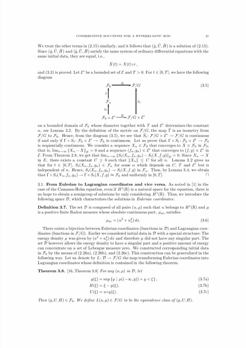
8/3/2019 Xavier Raynaud- On a Shallow Water Wave Equation
http://slidepdf.com/reader/full/xavier-raynaud-on-a-shallow-water-wave-equation 156/161
CONSERVATIVE SOLUTIONS FOR A HYPERELASTIC ROD 21
We treat the other terms in (2.15) similarly, and it follows that ( y, U , H ) is a solution of (2.15).
Since (y, U , H ) and (y, U , H ) satisfy the same system of ordinary differential equations with thesame initial data, they are equal, i.e.,
X (t) = X (t)◦r ,
and (3.3) is proved. Let E be a bounded set of E and T > 0. For t ∈ [0, T ], we have the followingdiagram
F 0 Π / / F /G
F αΓ
O O
F 0
× E
St
O O
Π / /
F /G
× E
St
O O(3.5)
on a bounded domain of F 0 whose diameter together with T and E determines the constantα, see Lemma 3.2. By the definition of the metric on F /G, the map Γ is an isometry from
F /G to F 0. Hence, from the diagram (3.5), we see that S t : F /G × E → F /G is continuousif and only if Γ ◦ S t : F 0 × E → F 0 is continuous. Let us prove that Γ ◦ S t : F 0 × E → F 0is sequentially continuous. We consider a sequence X n ∈ F 0 that converges to X ∈ F 0 in F 0,that is, limn→∞ X n − X E = 0 and a sequence (f n, gn) ∈ E that converges to (f, g) ∈ E inE . From Theorem 2.8, we get that limn→∞ S t(X n, f n, gn) − S t(X , f , g)E = 0. Since X n → X in E , there exists a constant C ≥ 0 such that X n ≤ C for all n. Lemma 3.2 gives usthat for t ∈ [0, T ], S t(X n, f n, gn) ∈ F α for some α which depends on C , T and E but isindependent of n. Hence, S t(X n, f n, gn) → S t(X , f , g) in F α. Then, by Lemma 3.4, we obtainthat Γ ◦ S t(X n, f n, gn) → Γ ◦ S t(X , f , g) in F 0 and uniformly in [0, T ].
3.1. From Eulerian to Lagrangian coordinates and vice versa. As noted in [1] in thecase of the Camassa-Holm equation, even if H 1(R) is a natural space for the equation, there isno hope to obtain a semigroup of solutions by only considering H 1(R). Thus, we introduce thefollowing space D, which characterizes the solutions in Eulerian coordinates:
Definition 3.7. The set D is composed of all pairs (u, µ) such that u belongs to H 1(R) and µis a positive finite Radon measure whose absolute continuous part, µac, satisfies
µac = (u2 + u2x) dx. (3.6)
There exists a bijection between Eulerian coordinates (functions in D) and Lagrangian coor-dinates (functions in F /G). Earlier we considered initial data in D with a special structure: Theenergy density µ was given by (u2 + u2
x) dx and therefore µ did not have any singular part. The
set D however allows the energy density to have a singular part and a positive amount of energycan concentrate on a set of Lebesgue measure zero. We constructed corresponding initial datain F 0 by the means of (2.26a), (2.26b), and (2.26c). This construction can be generalized in thefollowing way. Let us denote by L : D → F /G the map transforming Eulerian coordinates intoLagrangian coordinates whose definition is contained in the following theorem.
Theorem 3.8. [16, Theorem 3.8] For any (u, µ) in D, let
y(ξ) = sup {y | µ((−∞, y)) + y < ξ} , (3.7a)
H (ξ) = ξ − y(ξ), (3.7b)
U (ξ) = u◦y(ξ) . (3.7c)
Then (y,U,H )
∈ F 0. We define L(u, µ)
∈ F /G to be the equivalence class of (y,U,H ).
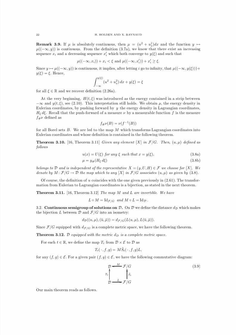
8/3/2019 Xavier Raynaud- On a Shallow Water Wave Equation
http://slidepdf.com/reader/full/xavier-raynaud-on-a-shallow-water-wave-equation 157/161
22 H. HOLDEN AND X. RAYNAUD
Remark 3.9. If µ is absolutely continuous, then µ = (u2 + u2x)dx and the function y →
µ((−∞, y)) is continuous. From the definition (3.7a), we know that there exist an increasingsequence xi and a decreasing sequence xi which both converge to y(ξ) and such that
µ((−∞, xi)) + xi < ξ and µ((−∞, xi)) + xi ≥ ξ.
Since y → µ((−∞, y)) is continuous, it implies, after letting i go to infinity, that µ((−∞, y(ξ)))+y(ξ) = ξ. Hence, y(ξ)
−∞(u2 + u2
x) dx + y(ξ) = ξ
for all ξ ∈ R and we recover definition (2.26a).
At the very beginning, H (t, ξ) was introduced as the energy contained in a strip between−∞ and y(t, ξ), see (2.10). This interpretation still holds. We obtain µ, the energy density inEulerian coordinates, by pushing forward by y the energy density in Lagrangian coordinates,H ξ dξ. Recall that the push-forward of a measure ν by a measurable function f is the measure
f #ν defined asf #ν (B) = ν (f −1(B))
for all Borel sets B. We are led to the map M which transforms Lagrangian coordinates intoEulerian coordinates and whose definition is contained in the following theorem.
Theorem 3.10. [16, Theorem 3.11] Given any element [X ] in F /G. Then, (u, µ) defined as follows
u(x) = U (ξ) for any ξ such that x = y(ξ), (3.8a)
µ = y#(H ξ dξ) (3.8b)
belongs to D and is independent of the representative X = (y,U,H ) ∈ F we choose for [X ]. Wedenote by M :
F /G
→ Dthe map which to any [X ] in
F /G associates (u, µ) as given by (3.8).
Of course, the definition of u coincides with the one given previously in (2.61). The transfor-mation from Eulerian to Lagrangian coordinates is a bijection, as stated in the next theorem.
Theorem 3.11. [16, Theorem 3.12] The map M and L are invertible. We have
L ◦ M = IdF /G and M ◦ L = IdD .
3.2. Continuous semigroup of solutions on D. On D we define the distance dD which makesthe bijection L between D and F /G into an isometry:
dD((u, µ), (u, µ)) = dF /G(L(u, µ), L(u, µ)).
Since F /G equipped with dF /G is a complete metric space, we have the following theorem.
Theorem 3.12. D equipped with the metric dD is a complete metric space.
For each t ∈ R, we define the map T t from D × E to D as
T t( · , f , g) = M S t( · , f , g)L,
for any (f, g) ∈ E . For a given pair (f, g) ∈ E , we have the following commutative diagram:
D F /GM o o
DT t
O O
L / / F /G
St
O O(3.9)
Our main theorem reads as follows.
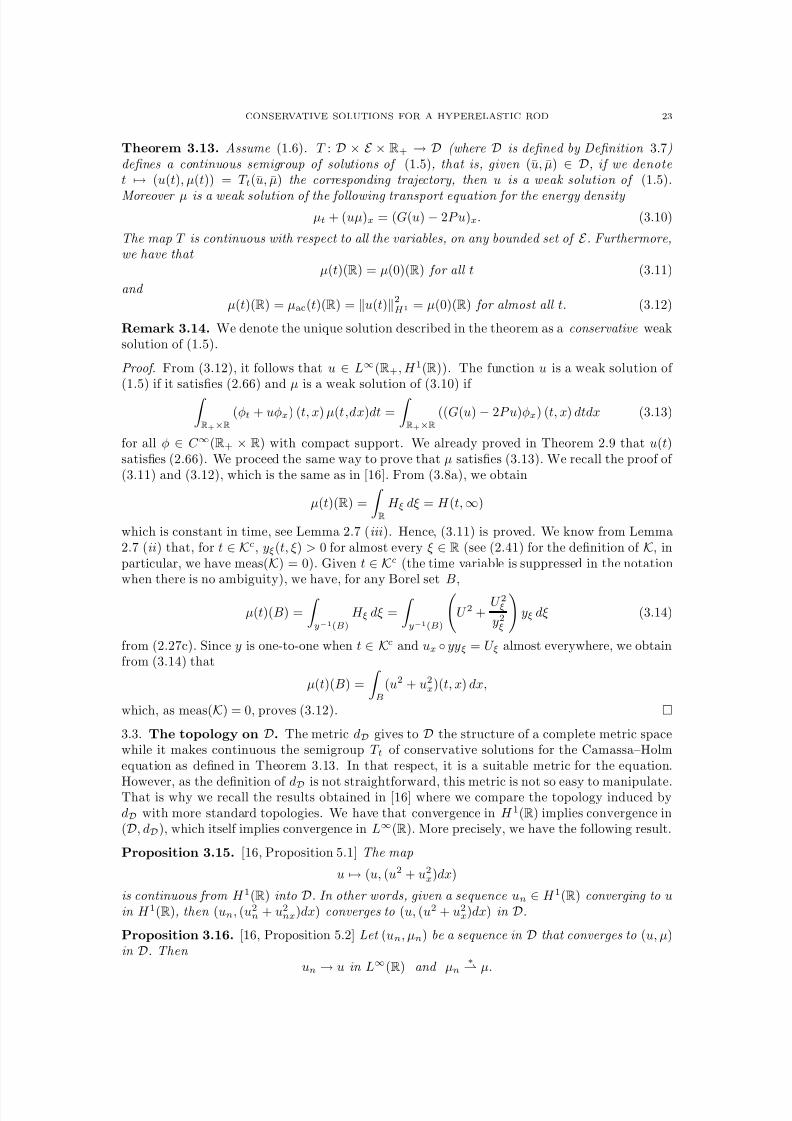
8/3/2019 Xavier Raynaud- On a Shallow Water Wave Equation
http://slidepdf.com/reader/full/xavier-raynaud-on-a-shallow-water-wave-equation 158/161
CONSERVATIVE SOLUTIONS FOR A HYPERELASTIC ROD 23
Theorem 3.13. Assume (1.6). T : D × E × R+ → D (where D is defined by Definition 3.7)defines a continuous semigroup of solutions of (1.5), that is, given (u, µ) ∈ D, if we denotet
→(u(t), µ(t)) = T t(u, µ) the corresponding trajectory, then u is a weak solution of (1.5).
Moreover µ is a weak solution of the following transport equation for the energy density µt + (uµ)x = (G(u) − 2P u)x. (3.10)
The map T is continuous with respect to all the variables, on any bounded set of E . Furthermore,we have that
µ(t)(R) = µ(0)(R) for all t (3.11)
and µ(t)(R) = µac(t)(R) = u(t)2
H 1 = µ(0)(R) for almost all t. (3.12)
Remark 3.14. We denote the unique solution described in the theorem as a conservative weaksolution of (1.5).
Proof. From (3.12), it follows that u ∈ L∞(R+, H 1(R)). The function u is a weak solution of (1.5) if it satisfies (2.66) and µ is a weak solution of (3.10) if
R+×R(φt + uφx) (t, x) µ(t,dx)dt =
R+×R
((G(u) − 2P u)φx) (t, x) dtdx (3.13)
for all φ ∈ C ∞(R+ × R) with compact support. We already proved in Theorem 2.9 that u(t)satisfies (2.66). We proceed the same way to prove that µ satisfies (3.13). We recall the proof of (3.11) and (3.12), which is the same as in [16]. From (3.8a), we obtain
µ(t)(R) =
R
H ξ dξ = H (t, ∞)
which is constant in time, see Lemma 2.7 (iii ). Hence, (3.11) is proved. We know from Lemma2.7 (ii ) that, for t ∈ Kc, yξ(t, ξ) > 0 for almost every ξ ∈ R (see (2.41) for the definition of K, inparticular, we have meas(K) = 0). Given t ∈ Kc (the time variable is suppressed in the notationwhen there is no ambiguity), we have, for any Borel set B,
µ(t)(B) =
y−1(B)
H ξ dξ =
y−1(B)
U 2 +
U 2ξy2ξ
yξ dξ (3.14)
from (2.27c). Since y is one-to-one when t ∈ Kc and ux ◦ yyξ = U ξ almost everywhere, we obtainfrom (3.14) that
µ(t)(B) =
B
(u2 + u2x)(t, x) dx,
which, as meas(K) = 0, proves (3.12).
3.3. The topology on D. The metric dD gives to D the structure of a complete metric spacewhile it makes continuous the semigroup T t of conservative solutions for the Camassa–Holmequation as defined in Theorem 3.13. In that respect, it is a suitable metric for the equation.
However, as the definition of dD is not straightforward, this metric is not so easy to manipulate.That is why we recall the results obtained in [16] where we compare the topology induced bydD with more standard topologies. We have that convergence in H 1(R) implies convergence in(D, dD), which itself implies convergence in L∞(R). More precisely, we have the following result.
Proposition 3.15. [16, Proposition 5.1] The map
u → (u, (u2 + u2x)dx)
is continuous from H 1(R) into D. In other words, given a sequence un ∈ H 1(R) converging to uin H 1(R), then (un, (u2
n + u2nx)dx) converges to (u, (u2 + u2
x)dx) in D.
Proposition 3.16. [16, Proposition 5.2] Let (un, µn) be a sequence in D that converges to (u, µ)in D. Then
un
→u in L∞(R) and µn
∗ µ.
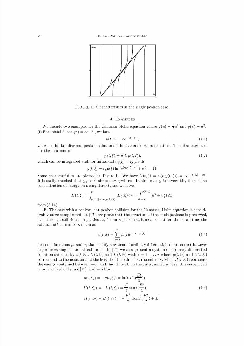
8/3/2019 Xavier Raynaud- On a Shallow Water Wave Equation
http://slidepdf.com/reader/full/xavier-raynaud-on-a-shallow-water-wave-equation 159/161
24 H. HOLDEN AND X. RAYNAUD
−15 0 15−10
0
10
ξ
time
Figure 1. Characteristics in the single peakon case.
4.Examples
We include two examples for the Camassa–Holm equation where f (u) = 12
u2 and g(u) = u2.
(i) For initial data u(x) = ce−|x|, we have
u(t, x) = ce−|x−ct|, (4.1)
which is the familiar one peakon solution of the Camassa–Holm equation. The characteristicsare the solutions of
yt(t, ξ) = u(t, y(t, ξ)), (4.2)
which can be integrated and, for initial data y(ξ) = ξ, yields
y(t, ξ) = sgn(ξ) ln
e(sgn(ξ)ct) + e|ξ| − 1
.
Some characteristics are plotted in Figure 1. We have U (t, ξ) = u(t, y(t, ξ)) = ce−|y(t,ξ)−ct|.
It is easily checked that yξ > 0 almost everywhere. In this case y is invertible, there is noconcentration of energy on a singular set, and we have
H (t, ξ) =
y−1((−∞,y(t,ξ)))
H ξ(η) dη =
y(t,ξ)
−∞(u2 + u2
x) dx,
from (3.14).(ii) The case with a peakon–antipeakon collision for the Camassa–Holm equation is consid-
erably more complicated. In [17], we prove that the structure of the multipeakons is preserved,even through collisions. In particular, for an n-peakon u, it means that for almost all time thesolution u(t, x) can be written as
u(t, x) =
n
i=1
pi(t)e−|x−qi(t)| (4.3)
for some functions pi and qi that satisfy a system of ordinary differential equation that howeverexperiences singularities at collisions. In [17] we also present a system of ordinary differentialequation satisfied by y(t, ξi), U (t, ξi) and H (t, ξi) with i = 1, . . . , n where y(t, ξi) and U (t, ξi)correspond to the position and the height of the ith peak, respectively, while H (t, ξi) representsthe energy contained between −∞ and the ith peak. In the antisymmetric case, this system canbe solved explicitly, see [17], and we obtain
y(t, ξ2) = −y(t, ξ1) = ln(cosh(Et
2)),
U (t, ξ2) = −U (t, ξ1) =E
2tanh(
Et
2),
H (t, ξ2)
−H (t, ξ1) =
−
E 2
2
tanh2(Et
2
) + E 2.
(4.4)
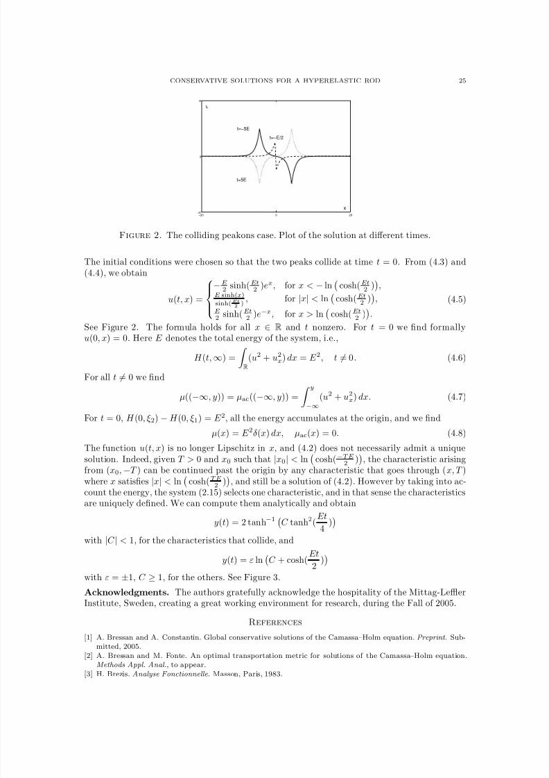
8/3/2019 Xavier Raynaud- On a Shallow Water Wave Equation
http://slidepdf.com/reader/full/xavier-raynaud-on-a-shallow-water-wave-equation 160/161
CONSERVATIVE SOLUTIONS FOR A HYPERELASTIC ROD 25
−20 0 20−E
0
E
t=−5E
t=−E/2
t=5E
u
x
Figure 2. The colliding peakons case. Plot of the solution at different times.
The initial conditions were chosen so that the two peaks collide at time t = 0. From (4.3) and
(4.4), we obtain
u(t, x) =
−E2
sinh(Et2
)ex, for x < − ln
cosh(Et2
)
,E sinh(x)
sinh(Et2
), for |x| < ln
cosh(Et
2)
,
E2 sinh(Et2 )e−x, for x > ln
cosh(Et2 )
.
(4.5)
See Figure 2. The formula holds for all x ∈ R and t nonzero. For t = 0 we find formallyu(0, x) = 0. Here E denotes the total energy of the system, i.e.,
H (t, ∞) =
R
(u2 + u2x) dx = E 2, t = 0. (4.6)
For all t = 0 we find
µ((−∞, y)) = µac((−∞, y)) = y
−∞
(u2 + u2x) dx. (4.7)
For t = 0, H (0, ξ2) − H (0, ξ1) = E 2, all the energy accumulates at the origin, and we find
µ(x) = E 2δ(x) dx, µac(x) = 0. (4.8)
The function u(t, x) is no longer Lipschitz in x, and (4.2) does not necessarily admit a uniquesolution. Indeed, given T > 0 and x0 such that |x0| < ln
cosh(−TE
2)
, the characteristic arisingfrom (x0, −T ) can be continued past the origin by any characteristic that goes through (x, T )where x satisfies |x| < ln
cosh(TE
2)
, and still be a solution of (4.2). However by taking into ac-count the energy, the system (2.15) selects one characteristic, and in that sense the characteristicsare uniquely defined. We can compute them analytically and obtain
y(t) = 2 tanh−1
C tanh2(Et
4)
with |C | < 1, for the characteristics that collide, andy(t) = ε ln
C + cosh(
Et
2)
with ε = ±1, C ≥ 1, for the others. See Figure 3.
Acknowledgments. The authors gratefully acknowledge the hospitality of the Mittag-LefflerInstitute, Sweden, creating a great working environment for research, during the Fall of 2005.
References
[1] A. Bressan and A. Constantin. Global conservative solutions of the Camassa–Holm equation. Preprint. Sub-mitted, 2005.
[2] A. Bressan and M. Fonte. An optimal transportation metric for solutions of the Camassa–Holm equation.Methods Appl. Anal., to appear.
[3] H. Brezis. Analyse Fonctionnelle. Masson, Paris, 1983.
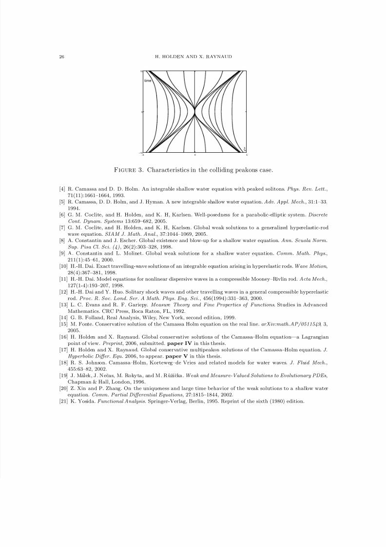
8/3/2019 Xavier Raynaud- On a Shallow Water Wave Equation
http://slidepdf.com/reader/full/xavier-raynaud-on-a-shallow-water-wave-equation 161/161
26 H. HOLDEN AND X. RAYNAUD
−5 0 5−10
0
10
ξ
time
Figure 3. Characteristics in the colliding peakons case.
[4] R. Camassa and D. D. Holm. An integrable shallow water equation with peaked solitons. Phys. Rev. Lett.,71(11):1661–1664, 1993.[5] R. Camassa, D. D. Holm, and J. Hyman. A new integrable shallow water equation. Adv. Appl. Mech., 31:1–33,
1994.[6] G. M. Coclite, and H. Holden, and K. H, Karlsen. Well-posedness for a parabolic-elliptic system. Discrete
Cont. Dynam. Systems 13:659–682, 2005.[7] G. M. Coclite, and H. Holden, and K. H, Karlsen. Global weak solutions to a generalized hyperelastic-rod
wave equation. SIAM J. Math. Anal., 37:1044–1069, 2005.[8] A. Constantin and J. Escher. Global existence and blow-up for a shallow water equation. Ann. Scuola Norm.
Sup. Pisa Cl. Sci. (4), 26(2):303–328, 1998.[9] A. Constantin and L. Molinet. Global weak solutions for a shallow water equation. Comm. Math. Phys.,
211(1):45–61, 2000.[10] H.-H. Dai. Exact travelling-wave solutions of an integrable equation arising in hyperelastic rods. Wave Motion ,
28(4):367 381 1998