Zoom and Learn: Generalizing Deep Stereo Matching to Novel Domains

Jiahao Pang1 Wenxiu Sun1 Chengxi Yang1 Jimmy Ren1 Ruichao Xiao1 Jin Zeng1 Liang Lin1,2

1SenseTime Research 2Sun Yat-sen University{pangjiahao, sunwenxiu, yangchengxi, rensijie, xiaoruichao, zengjin, linliang}@sensetime.com

Abstract

Despite the recent success of stereo matching with con-volutional neural networks (CNNs), it remains arduous togeneralize a pre-trained deep stereo model to a novel do-main. A major difficulty is to collect accurate ground-truth disparities for stereo pairs in the target domain. Inthis work, we propose a self-adaptation approach for CNNtraining, utilizing both synthetic training data (with ground-truth disparities) and stereo pairs in the new domain (with-out ground-truths). Our method is driven by two empiricalobservations. By feeding real stereo pairs of different do-mains to stereo models pre-trained with synthetic data, wesee that: i) a pre-trained model does not generalize well tothe new domain, producing artifacts at boundaries and ill-posed regions; however, ii) feeding an up-sampled stereopair leads to a disparity map with extra details. To avoidi) while exploiting ii), we formulate an iterative optimiza-tion problem with graph Laplacian regularization. At eachiteration, the CNN adapts itself better to the new domain:we let the CNN learn its own higher-resolution output; atthe meanwhile, a graph Laplacian regularization is imposedto discriminatively keep the desired edges while smoothingout the artifacts. We demonstrate the effectiveness of ourmethod in two domains: daily scenes collected by smart-phone cameras, and street views captured in a driving car.

1. IntroductionStereo matching is a classic yet important problem for

many computer vision tasks (e.g., 3D reconstruction [7] andautonomous vehicles [6]). Particularly, given a rectified im-age pair captured by stereo cameras, one aims at estimatingthe disparity of each pixel between the two images. Tra-ditionally, a stereo matching pipeline starts from matchingcost computation and cost aggregation. Further optimiza-tion and refinement lead to the output disparity [13]. Recentadvances in deep learning has inspired a lot of end-to-endconvolutional neural networks (CNNs) for stereo matching,e.g., [18, 23]. Unlike the traditional wisdom, an end-to-endCNN integrates the stereo matching pipeline into a holisticdeep architecture by learning from the training data. Under

confined scenarios with proper training data (e.g., the KITTIdataset [6]), the end-to-end deep stereo models achieve un-precedented state-of-the-art performance.

However, it remains difficult to generalize a pre-traineddeep stereo model to a novel scenario. Firstly, the con-tents in the source domain may have very different char-acteristics from the target domain. Moreover, real stereopairs collected with different stereo modules suffer fromseveral degenerations—e.g., noise corruption, photometricdistortions, imperfections in rectification—to different ex-tents. Directly feeding a stereo pair of the target domain to aCNN pre-trained from another domain deteriorates its per-formance significantly. Consequently, state-of-the-art ap-proaches, e.g., [18, 28], train their models with syntheticdatasets [23], then perform finetuning on a fewer amountof domain-specific data with ground-truths. Unfortunately,besides a few public datasets for research purpose, e.g., theKITTI dataset [6] and the Middlebury dataset [32], it is ex-pensive and troublesome to collect real stereo pairs with ac-curate ground-truth disparities.

To resolve this dilemma, we propose a self-adaptationapproach to generalize deep stereo matching methods tonovel domains. We utilize synthetic training data and stereopairs of the target domain, where only the synthetic datahave known disparity maps. Our approach is compatiblewith end-to-end deep stereo methods, e.g., [23, 28], guidinga pre-trained model to gradually adapt to the target scenario.We start our explorations by feeding real stereo pairs fromdifferent domains to models pre-trained with synthetic data,resulting in two empirical observations:

(i) Generalization glitches: a pre-trained model does notgeneralize well on the target domain—the produceddisparity maps can be blurry at object edges and erro-neous at ill-posed regions;

(ii) Scale diversity: feeding a properly up-sampled stereopair (the same stereo pair at a finer scale) leads toanother disparity map with more meaningful details,e.g., sharper object boundaries, more high-frequencycontents of the scene.

To avoid the issues of (i) while exploiting the benefits of (ii),

1

arX

iv:1

803.

0664

1v1

[cs

.CV

] 1

8 M

ar 2

018

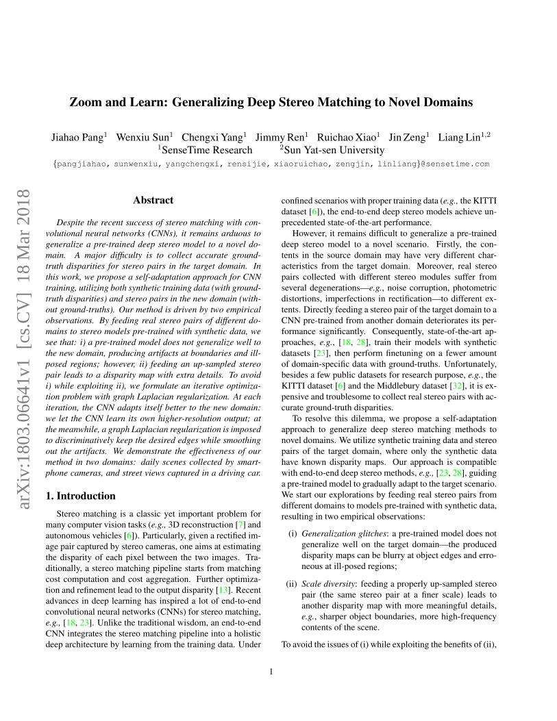
Left DispNetC DispNetC-80 Ours

Figure 1. Feeding stereo pairs collected from smartphones to mod-els pre-trained from synthetic data leads to blurry edges and arti-facts. In contrast, our self-adaptation approach brings significantimprovements to the disparity maps.

we propose an iterative regularization scheme for finetuningdeep stereo matching models.

We formulate the CNN training as an iterative optimiza-tion problem with graph Laplacian regularization. On onehand, we let the CNN learn its own finer-grain output; onthe other hand, a graph Laplacian regularization is imposedto discriminatively retain the useful edges while smooth-ing out the undesired artifacts. Our formulation, composingof a data term and a smoothness term, is solved iteratively,leading to a model well suited for the novel domain e.g.,Figure 1. The proposed self-adaptation approach is calledzoom and learn, or ZOLE, for short. We demonstrate the ef-fectiveness of our approach to two different domains: dailyscenes collected by smartphone cameras, and street viewscaptured from the perspective of a driving car.

This paper is structured as follows. Related works arereviewed in Section 2. We then illustrate our observationsabout deep stereo models in Section 3. The proposed self-adaptation approach is introduced in Section 4. Section 5presents the experimental results and Section 6 concludesour work.

2. Related Works

We first review several stereo matching algorithms basedon convolutional neural networks (CNNs). We then turn torelated works on graph Laplacian regularization and itera-tive regularization/filtering.

Deep stereo algorithms: Recent breakthroughs in deeplearning have reshaped the paradigms of many computervision tasks, including stereo matching. Early works em-ploying CNNs for stereo matching focuses on learning a ro-

bust similarity measure for matching cost computation e.g.,[11, 37]. To produce disparity maps, modules in the tra-ditional stereo matching pipeline are indispensable. Theremarkable work, DispNet, proposed by Mayer et al [23],is the first end-to-end CNN approach for stereo matching,where an encoder-decoder architecture is employed for su-pervised learning. Other recent works with leading per-formance include CRL [28], GC-NET [18], DRR [8], etc.These works explore different CNN architectures tailor-made for stereo matching. They achieve superior resultson the KITTI 2015 stereo benchmark [6], a benchmark con-taining driving scenes. Despite the success of these method-ologies, to adopt them in a novel domain, it is necessary tofine-tune the models with new domain-specific data. Unfor-tunately, in practice, it is very difficult to collect accuratedisparity maps for training [6, 32].

To mitigate this problem, some recent works proposedsemi-/un-supervised approaches to train a CNN model forstereo matching (or its related problem, monocular depthestimation). This category of works is essentially based onleft-right consistency/warping, e.g., [10, 19, 38, 39]. Forinstance, one may synthesize the left (or right) view ac-cording to the estimated left (or right) disparity and theright (or left) view for computing a loss function. However,left-right consistency becomes vulnerable when the stereopairs are imperfect, e.g., when the two views have differ-ent photometric distortions. Another line of research byTonioni et al. [34] propose to finetune a pre-trained modelto achieve domain adaptation. Their method relies on theresults of other stereo methods and confidence measures.Our work also performs finetuning with a pre-trained stereomodel. In contrast, we do not rely on external models orsetups: our self-supervised domain adaptation method letsthe CNN discriminatively learn the useful details from itsown finer-grain outputs.

Other related works: According to [21, 33], graphLaplacian regularization is particularly useful for the recov-ery of piecewise smooth signals, e.g., disparity maps. Byhaving an appropriate graph, edges can be preserved whileundesired defects are suppressed [26, 27]. Hence, we pro-pose to apply graph Laplacian regularization to selectivelylearn and preserve the meaningful details from the higher-resolution disparity outputs.

Iterative regularization/filtering is an important tech-nique in classic image restoration [17, 24, 25]. To restore acorrupted image, it is regularized iteratively through a vari-ational formulation, so that its quality improves at each it-eration. To utilize scale diversity while avoiding general-ization glitches (as mentioned in Section 1), we embed iter-ative regularization into the CNN training process, makingthe model parameters improve gradually. Different from it-erative refinement via a stacked neural network architecture,e.g., [15, 35], our iterative process occurs during training.

3. Observations

We first present two phenomena by feeding real-worldstereo pairs in different domains to deep stereo models pre-trained with synthetic datasets (e.g., FlyingThings3D [23],MPI Sintel [3], Virtual KITTI [5]). Underlying reasonsfor these phenomena will also be presented. We choosethe off-the-shelf DispNet [23] architectures—both the onewith explicit correlation (DispNetC) and the one based onconvolution only (DispNetS)—for our discussions. Theirencoder-decoder architectures are representative and alsowidely used in the deep learning literature, e.g., [1, 22, 31].

3.1. Generalization Glitches

In general, a stereo model pre-trained with synthetic datadoes not perform well on real stereo data in a particular do-main. Firstly, the contents of the synthetic data may dif-fer from that of the target domain. Moreover, real stereopairs inevitably suffer from defects arising from the imag-ing process. For instance, they are likely corrupted by noise.Besides, the two views may have different photometric dis-tortions due to inconformity of the two cameras. In somecases, the stereo pair may not even be well rectified, e.g.,two corresponding pixels are not on the same scan-line. Allthe above factors deteriorate the performance of a modelpre-trained with synthetic data.

For illustration, we use smartphones equipped withtwo rear-facing cameras to collect a few stereo pairs (ofsize 1024×1024), then perform the following tests. Wefirst adopt the released DispNetC model pre-trained withthe FlyingThings3D dataset [23]. Since stereo pairs ofsmartphones have small disparity values, we also fine-tune a model from the released model, where we removethose FlyingThings3D stereo pairs with maximum disparitylarger than 80. Data augmentation is introduced for the twoviews individually during training, please refer to Section 5for more details. The resulting model is called DispNetC-80. Both DispNetC and DispNetC-80 perform very wellon the FlyingThings3D dataset, but are problematic whenapplied to real smartphone data. Figure 1 shows a few dis-parity estimates of DispNetC and DispNetC-80. As can beseen, the results are blurry at object edges. Moreover, atill-posed regions, i.e., object occlusions, repeated patterns,and textureless regions, the disparity maps are erroneous.In this work we call this generalization glitches, meaningthe mistakes that a deep stereo model (pre-trained with syn-thetic data) make when it is applied to real stereo pairs of acertain domain.

3.2. Scale Diversity

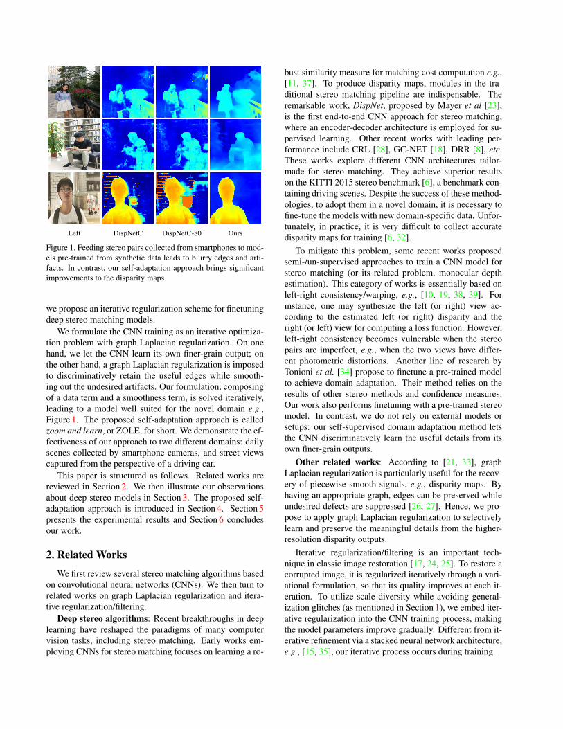
In spite of the unpleasant generalization glitches, we findthat deep stereo models have an encouraging property. Sup-pose we have a stereo pair P = (L,R), where L and R are

Figure 2. For the same stereo pair, feeding its zoomed-in version toa stereo matching CNN leads to a disparity map with extra details.The four rows are the left image, the disparity maps obtained by(1), with up-sampling ratio r = 1, 1.5, 2, respectively.

the left and the right views, respectively. We denote a deepstereo model parameterized by Θ as S(·;Θ). By applying itto the stereo pair P leads to a disparity map D = S (P ;Θ).The operation of up-sampling by r times is denoted as ↑r(·)while down-sampling by r times is ↓r(·). By passing an up-sampled stereo pair to S then down-sampling the result, weobtain another disparity map, D′, of the same size as D,

D′ =1

r· ↓r (S (↑r(P );Θ)) . (1)

Note that after downsampling, the factor 1/r is necessaryfor making D′ to have the correct scaling. Compared toD, D′ usually contains more high-frequency details. To seethis, we apply the released DispNetC model to a few stereopairs captured by smartphones. We make the original sizeof the stereo pairs as 640× 640. For each of them, we esti-mate three disparity maps based on (1) with r ∈ {1, 1.5, 2}.Visual results are shown in Figure 2. We see that as r grows,more fine details are produced on the disparity maps.

However, a bigger r does not necessarily mean better re-sults. For further inspection, we adopt the released Disp-NetC and DispNetS models (trained with the FlyingTh-ings3D dataset) and measure their performance on the train-ing set of KITTI stereo 2015 [6] at different resolutions.The results, in terms of the percentage of pixels with an er-ror greater than 3, or three-pixel error rate (3ER), are listed

Table 1. The average three-pixel error rates of the released Disp-NetC and DispNetS models on the training set of KITTI stereo2015. A resolution of N means the stereo pairs are resized toN ×N before passing to the CNNs.

NetworkResolution

896 1280 1664 2048 2432DispNetC 14.26% 9.97% 8.81% 9.17% 10.53%DispNetS 18.95% 11.61% 9.18% 8.64% 9.08%

in Table 1. We see that as the input resolution increases, theperformance first improves then deteriorates. Because:

(i) Up-sampling the stereo pairs enables the model to per-form stereo matching at a localized manner with sub-pixel accuracy. Hence, more details on the stereo pairsare taken into account for computation, leading to dis-parity estimates with extra high-frequency contents;

(ii) A finer-scale input translates to a smaller effectivesearch range (or receptive field). As a CNN becomestoo “short-sighted,” it lacks non-local information toestimate a proper disparity map, and its performancestart to decline.

This phenomenon—different results can be observed withdifferent input scales—is called scale diversity, akin to theconcept of transmit diversity in communication [30]. Wefind that scale diversity also exists in other problems, e.g.,optical flow estimation [15, 23] and image segmentation[22], please refer to the supplementary material for moredetails.

4. Zoom and LearnTo achieve effective self-adaptation, our approach—

zoom and learn (ZOLE)—finetunes a model pre-trainedwith synthetic data. It iteratively suppresses generalizationglitches while utilizing the benefits of scale diversity.

4.1. Graph Laplacian Regularization

Graph Laplacian regularization is employed in a widerange of image restoration literature, e.g., [4, 9, 24]. It isalso proven to be effective for the recovery of piecewisesmooth signals [14, 26, 33]. We adopt graph Laplacian reg-ularization (on a patch-by-patch basis) to guide the learn-ing of CNNs. Graph Laplacian regularization assumes theground-truth signal s ∈ Rm—in our case, a patch on theground-truth disparity—is smooth with respect to a pre-defined graph G with m vertices. Specifically, it imposesthat the value of sTLs, i.e., the graph Laplacian regular-izer, should be small for the ground-truth patch s, whereL ∈ Rm×m is the graph Laplacian matrix of graph G.Given a disparity map D produced by a deep stereo model,we compute the values of the graph Laplacian regularizers

for the patches on D. The obtained values are summed upas a graph Laplacian regularization loss for CNN training.

For an effective regularization with graph Laplacian, it iscritical to constructing a graph G properly. We employ thegraph structure of [12, 26] which works well for disparitymap denoising. For illustration, we first introduce the con-cept of exemplar patches. Exemplar patches are a set of Kpatches, fk ∈ Rm where 1 ≤ k ≤ K, that are statisticallyrelated to the ground-truth patch s. For instance, an exem-plar patch can be a rough estimate of s, or the co-locatedpatch on the left image, etc. Our choices of the exemplarpatches will be presented in Section 4.2. With the exemplarpatches, the edge weight wij connecting pixel i and pixel jon patch s is given by

wij =

{exp

(−d2

ij

)if |dij | ≤ ε,

0 otherwise,

where ε is a threshold, d2ij is a distance measure between

pixel i and pixel j. Hence, the resulting graph G is an ε-neighborhood graph, i.e., there is no edge connecting twopixels with a distance greater than ε. We choose an indi-vidual value of ε for each patch, making every vertex of thegraph has at least 4 edges. The distance measure d2

ij is de-fined as follows:

d2ij =

∑K

k=1(fk(i)− fk(j))

2+ α · l2ij , (2)

where fk(i) and fk(j) denote the i-th and the j-th entriesof fk, respectively, so the first term of (2) measures the Eu-clidean distance between pixels i and j in a K-dimensionalspace defined by the exemplar patches. lij is simply thespatial distance (length) between pixels i and j, and α is aconstant weight, empirically set to be a small value 0.2.

The adjacency matrix of G is denoted as A, where the(i, j)-th entry of A is wij . The degree matrix of G is a di-agonal matrix D, its i-th diagonal entry is

∑mj=1 wij . Then

the graph Laplacian L is given by L = D − A, leadingto the graph Laplacian regularizer sTLs ∈ R. From theanalysis of [26], graph Laplacian regularizer is an adaptivemetric. If the same edge (or gradient ) pattern appears inthe majority of the exemplar patches, minimizing the graphLaplacian regularizer promotes the very edge pattern; if theexemplar patches are inconsistent, graph Laplacian regular-ization leads to a smoothed patch. We exploit this propertyto guide a deep stereo model to selectively learn the desireddetails.

4.2. Training by Iterative Regularization

We borrow the notion of iterative regularization [24] forgeneralizing deep stereo models to novel domains, givingrise to the proposed zoom and learn approach. Supposewe have a deep stereo model S(·;Θ(0)) (parameterized byΘ(0)) pre-trained with synthetic data. We also have a set

of N stereo pairs, Pi = (Li, Ri), 1 ≤ i ≤ N , where thefirst Ndom of them are real stereo pairs of the target domainwhile the rest Nsyn = N − Ndom pairs are synthetic data,among which only the synthetic data has ground truth dis-parities Di (Ndom + 1 ≤ i ≤ N ).

We solve for a new set of model parameters Θ(k+1) atiteration k. For a constant r > 1, we first create a set of“ground-truths” for the Ndom real stereo pairs by zooming(up-sampling), i.e.,

Di =1

r· ↓r

(S(↑r(Pi);Θ

(k)))

, 1 ≤ i ≤ Ndom. (3)

From Section 3.2, Di contains more details thanS(Pi;Θ

(k)). We divide a disparity map Di into Msquare patches tiling it where each patch is a vector oflength m. The vectorization operator is denoted as vec(·)so that vec(Di) ∈ RMm. The m-by-Mm matrix extractingthe j-th patch from Di is denoted as Rj . With thesesettings, we formulate the following iterative optimizationproblem,

Θ(k+1) = argminΘ

Ndom∑i=1

M∑j=1

‖sij − dij‖1+λ · sTijL

(k)ij sij+

τ ·N∑

i=Ndom+1

‖S(Pi;Θ)−Di‖1, (4)

s.t. sij = Rj · vec (S(Pi;Θ)) , dij = Rj · vec (Di) .

Here sij and dij are the j-th patches of S(Pi;Θ) and Di,respectively. λ and τ are positive constants. Our optimiza-tion problem (4) first minimizes over each patch on theNdom stereo pairs: the first term (data term) drives sij tobe similar to dij ; and the second term (smoothness term) isa graph Laplacian regularizer induces from the matrix L

(k)ij .

The third term of (4) lets Θ(k+1) be a feasible deep stereomodel; it literally means that: a deep stereo model workswell for the target domain should also has reasonable per-formance on the synthetic data.

At iteration k, a graph G(k)ij (1 ≤ i ≤ Ndom, 1 ≤ j ≤

M ), and hence the corresponding graph Laplacian, L(k)ij , are

pre-computed for calculating a loss sTijL

(k)ij sij . We choose

the following three exemplar patches for building G(k)ij :

fleft = wleft · Rj · vec(Li),

fcurr = wcurr · Rj · vec(S(Pi;Θ(k))),

ffine = wfine · Rj · vec(Di) = wfine · dij ,

where wleft, wcurr and wfine are constants. In other words,fleft, fcurr, and ffine are the j-th patches of the left imageLi, the current prediction S(Pi;Θ

(k)) and the finer-grainprediction Di (3), respectively.

Our chosen exemplar patches lead to a graph Laplacianregularizer that discriminatively retain the desired detailsfrom ffine whilst smoothing out possible artifacts on bothfcurr and ffine. We analyze how the patches fleft, fcurr andffine affects the behavior of the graph Laplacian:

(i) Suppose a desired object boundary (denoted by A)does not appear in the current predicted patch fcurr.However, it has appeared in the finer-grain patchffine by virtue of scale diversity (Section 3.2), then Ashould also appear in fleft; otherwise the CNN cannotgenerate A on ffine. In this case, both ffine and fleft

have boundary A, resulting in a Laplacian L(k)ij that

promotes A on sij .

(ii) Suppose due to generalization glitches, an undesiredpattern (denoted as B) is produced in one exemplarpatch, fcurr or ffine. Since B is absence in the otherexemplar patches, the corresponding graph LaplacianL

(k)ij penalizes B on sij .

Hence, our graph Laplacian regularizer guides the CNN toonly learn the meaningful details.

4.3. Practical Algorithm

Iteratively solving the optimization problem (4) can beachieved by training the model S(·;Θ) with standard back-propagation [20]. We hereby present how to use the pro-posed formulation for finetuning a pre-trained model inpractice. Since a disparity map Di is tiled by M patches,dij with 1 ≤ j ≤ M , the first term in (4) equals∑Ndom

i=1 ‖S(Pi;Θ)−Di‖1. Hence, the objective of (4) canbe rewritten as:

Θ(k+1) = argminΘ

Ndom∑i=1

‖S(Pi;Θ)−Di‖1+

τ ·N∑

i=Ndom+1

‖S(Pi;Θ)−Di‖1 + λ ·Ndom∑i=1

M∑j=1

sTijL

(k)ij sij ,

(5)

We see that the first two terms of (5) are simply L1 losswith different weightings for the target domain and the syn-thetic data. The third term is the proposed graph Laplacianregularization loss, we discuss its backpropagation in thesupplementary material.

In general, there are a lot of training examples (N islarge), yet in practice, every training iteration can onlytake in a batch of n � N training examples and performstochastic gradient descent. As a result, we shuffle all theN stereo pairs and sequentially take out n of them to form atraining batch for the current iteration. For a synthetic stereopair Pi (Ndom + 1 ≤ i ≤ N ) in the batch, we directly useits L1 loss for backpropagation since its ground-truth Di is

Algorithm 1 Zoom and learn (ZOLE)1: Input: Pre-trained deep stereo model S(·;Θ(0)),

training data {Pi}Ndomi=1 and {Pi, Di}Ni=Ndom+1

2: Shuffle the training data to form a list `3: for k = 0 to kmax − 1 do4: for b = 1 to n do5: Draw an index i from list `6: if i ≤ Ndom then7: Compute Di, then compute S(Pi;Θ

(k)) and hencethe graph Laplacian matrices L

(k)ij

8: end if9: Insert {Pi, Di} to the current batch

10: end for11: Use the formed training batch and the pre-computed Lapla-

cian matrices to perform a step of gradient descent12: if mod(k + 1, t) = 0 then13: Perform validation, update Θ(bst) and v(bst) if needed14: end if15: end for16: Output: model parameters Θ(bst)

known. Otherwise, for a stereo pair Pi with 1 ≤ i ≤ Ndom

in the batch, we first feed its up-sampled version to theCNN for computing the finer-grain “ground-truth” Di, wealso compute the current estimate S(Pi;Θ

(k)) and hencethe graph Laplacian matrices L

(k)ij for each patch. With Di

and the pre-computed L(k)ij ’s, 1 ≤ j ≤ M , both the L1 loss

and the graph Laplacian regularization loss are employedfor backpropagation.

For every t training iterations, we perform a validationprocedure with left-right consistency, using another set ofN

(v)dom stereo pairs in the target domain. We first estimate the

disparity maps with the up-to-date model then synthesizeN

(v)dom left images with the estimated disparity maps and the

right images. Then we compute the peak signal-to-noiseratios (PSNRs) between the synthesized left images and thegenuine ones. The average PSNR reflects the performanceof the current model. During the training process, we keeptrack of the best PSNR value v(bst) and its correspondingmodel Θ(bst). After kmax training iterations, we terminatethe training and output Θ(bst). Algorithm 1 summarizes thekey steps of our self-adaptation approach.

5. Experimentation

In this section, we generalize deep stereo matching fortwo different domains in the real world: daily scenes cap-tured by smartphone cameras, and street views from theperspective of a driving car (the KITTI dataset [6]). Weagain choose the representative DispNetC [23] architecturefor our experiments.

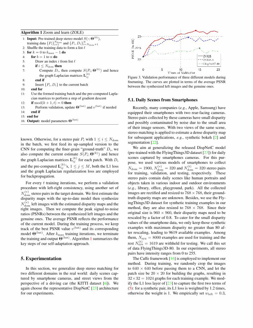
Figure 3. Validation performance of three different models duringfinetuning. The curves are plotted in terms of the average PSNRbetween the synthesized left images and the genuine ones.

5.1. Daily Scenes from Smartphones

Recently, many companies (e.g., Apple, Samsung) haveequipped their smartphones with two rear-facing cameras.Stereo pairs collected by these cameras have small disparityand possibly contaminated by noise due to the small areaof their image sensors. With two views of the same scene,stereo matching is applied to estimate a dense disparity mapfor subsequent applications, e.g., synthetic bokeh [2] andsegmentation [22].

We aim at generalizing the released DispNetC model(pre-trained with the FlyingThings3D dataset [23]) for dailyscenes captured by smartphones cameras. For this pur-pose, we used various models of smartphones to collectNdom = 1900, N (v)

dom = 320 and N (t)dom = 320 stereo pairs

for training, validation, and testing, respectively. Thesestereo pairs contain daily scenes like human portraits andobjects taken in various indoor and outdoor environments(e.g., library, office, playground, park). All the collectedimages are rectified and resized to 768× 768, their ground-truth disparity maps are unknown. Besides, we use the Fly-ingThings3D dataset for synthetic training examples in ourmethod, they are also resized to 768 × 768. Since theiroriginal size is 960 × 960, their disparity maps need to berescaled by a factor of 0.8. To cater for the small disparityvalues of the smartphone data, we only keep those syntheticexamples with maximum disparity no greater than 80 af-ter rescaling, leading to 9619 available examples. Amongthem, Nsyn = 8000 examples are used for training and therest N (t)

syn = 1619 are withheld for testing. We call this setof data FlyingThings3D-80. In our experiments, all stereopairs have intensity ranges from 0 to 255.

The Caffe framework [16] is employed to implement ourmethod. During training, we randomly crop the imagesto 640 × 640 before passing them to a CNN, and let thepatch size be 20 × 20 for building the graphs, resulting in32×32 = 1024 graphs for each training example. We mod-ify the L1 loss layer of [23] to capture the first two terms of(5): for a synthetic pair, its L1 loss is weighted by 1.2 times,otherwise the weight is 1. We empirically set wleft = 0.3,

Left image Tonioni et al. [34] DispNetC ZOLE-S ZOLE

Figure 4. Visual comparisons of several models on the test set of our smartphone data. This figure shows fragments of left images and thecorresponding disparity maps obtained with different models. It is clear that our ZOLE approach produces superior disparity results.

Table 2. Performance comparison of our obtained zoom and learn (ZOLE) model and the other four models.

Dataset MetricModel

Tonioni [34] DispNetC DispNetC-80 ZOLE-S ZOLE

Smartphone PSNR SSIM 22.92 0.845 21.99 0.790 22.39 0.817 22.84 0.851 23.12 0.855FlyingThings3D-80 EPE 3ER 1.08 6.79% 1.03 5.63% 0.93 5.11% 1.10 6.88% 1.11 6.54%

wfine = 0.8 and wcurr = 1, all the computed sTijL

(k)ij sij

are averaged then weighted by 1.5 times for a loss (the thirdterm in (5)). We have tried out different up-sampling ratiosr’s ranging from 1.2 to 2 for computing Di, and found thethe obtained CNNs have similar performance. In our exper-iments, we let r = 1.5. Data augmentation is introducedto the synthetic stereo pairs. For each individual view ina synthetic pair, Gaussian noise (σ ∈ {0, 10, 15}) are ran-domly added. The brightness of each image channel arealso randomly adjusted (by a factor of ρ ∈ {0.8, 1, 1.2}).We let the batch size be 6, the learning rate be 5 × 10−5,and finetune the model for kmax = 104 iterations, valida-tion is performed every 500 iterations.

We first study the following models:(i) ZOLE: Generalize the pre-trained model for smart-

phone stereo pairs with our method;

(ii) ZOLE-S: Remove graph regularization and simply letthe CNN iteratively learn its own finer-grain outputs;

(iii) DispNetC-80: Finetune the pre-trained model on theFlyingThings3D-80 examples;

(iv) DispNetC: Released model pre-trained with Fly-ingThings3D [23].

The very recent method [34] by Tonioni et al. also fine-tunes a pre-trained model using stereo pairs from the targetdomain. They first estimate disparity maps for the target do-main with AD-CENCUS [36]. To finetune the model, theytreat the obtained disparity maps as “ground-truths” whiletaking a confidence measure [29] into account. For com-parison, we finetune a model with their released code undertheir recommended settings.

Since the stereo pairs of smartphones do not haveground-truth disparities, we evaluate the performance of amodel in a way similar to the validation process presentedin Section 4.3. We synthesize the left images with the esti-mated disparities and the right images, then measure the dif-ference between the synthesized left images and the genuineones, using both PSNR and SSIM as the difference metrics.For testing or validation, all the stereo pairs are fed to theCNN at a fixed resolution of 1024×1024. Figure 3 plots theperformance of ZOLE, ZOLE-S and DispNetC-80 on thevalidation set of the smartphone data during training (mea-sured in terms of average PSNR of the synthesized left im-ages). Besides, Table 2 presents the performance of all theaforementioned models, on both the test sets of the smart-phone data and FlyingThings3D-80. We use end-point-

Left image Tonioni et al. [34] DispNetC ZOLE

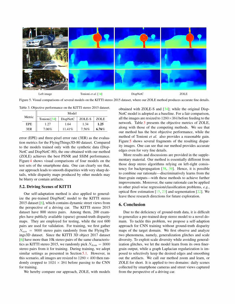
Figure 5. Visual comparisons of several models on the KITTI stereo 2015 dataset, where our ZOLE method produces accurate fine details.

Table 3. Objective performance on the KITTI stereo 2015 dataset.

MetricModel

Tonioni [34] DispNetC ZOLE-S ZOLEEPE 1.27 1.64 1.34 1.253ER 7.06% 11.41% 7.56% 6.76%

error (EPE) and three-pixel error rate (3ER) as the evalua-tion metrics for the FlyingThings3D-80 dataset. Comparedto the models trained only with the synthetic data (Disp-NetC and DispNetC-80), the one obtained with our method(ZOLE) achieves the best PSNR and SSIM performance.Figure 4 shows visual comparisons of four models on thetest sets of the smartphone data. One can clearly see that,our approach leads to smooth disparities with very sharp de-tails, while disparity maps produced by other models maybe blurry or contain artifacts.

5.2. Driving Scenes of KITTI

Our self-adaptation method is also applied to general-ize the pre-trained DispNetC model to the KITTI stereo2015 dataset [6], which contains dynamic street views fromthe perspective of a driving car. The KITTI stereo 2015dataset have 800 stereo pairs. Among them, 200 exam-ples have publicly available (sparse) ground-truth disparitymaps. They are employed for testing, while the rest 600pairs are used for validation. For training, we first gatherNsyn = 9000 stereo pairs randomly from the FlyingTh-ings3D dataset. Since the KITTI 3D object 2017 dataset[6] have more than 10k stereo pairs of the same characteris-tics as KITTI stereo 2015, we randomly pick Ndom = 3000stereo pairs from it for training. During training, we adoptsimilar settings as presented in Section 5.1. However, inthis scenario, all images are resized to 1280× 400 then ran-domly cropped to 1024 × 384 before passing to the CNNfor training.

We hereby compare our approach, ZOLE, with models

obtained with ZOLE-S and [34]; while the original Disp-NetC model is adopted as a baseline. For a fair comparison,all the images are resized to 1280×384 before feeding to thenetwork. Table 3 presents the objective metrics of ZOLE,along with those of the competing methods. We see thatour method has the best objective performance, while themethod of Tonioni et al. also provides a reasonable gain.Figure 5 shows several fragments of the resulting dispar-ity images. One can see that our method provides accurateedges even for very fine details.

More results and discussions are provided in the supple-mentary material. Our method is essentially different fromthose deep stereo algorithms relying on left-right consis-tency for backpropagation [38, 39]. Hence, it is possibleto combine our rationale—discriminatively learns from thefiner-grain outputs—with these methods to achieve furtherimprovements. Moreover, the same rationale can be appliedto other pixel-wise regression/classification problems, e.g.,optical flow estimation [15, 23] and segmentation [22]. Weleave these research directions for future exploration.

6. ConclusionDue to the deficiency of ground-truth data, it is difficult

to generalize a pre-trained deep stereo model to a novel do-main. To tackle this problem, we propose a self-adaptionapproach for CNN training without ground-truth disparitymaps of the target domain. We first observe and analyzetwo phenomena, namely, generalization glitches and scalediversity. To exploit scale diversity while avoiding general-ization glitches, we let the model learn from its own finer-grain output, while a graph Laplacian regularization is im-posed to selectively keep the desired edges and smoothingout the artifacts. We call our method zoom and learn, orZOLE for short. It is applied to two domains: daily scenescollected by smartphone cameras and street views capturedfrom the perspective of a driving car.

References[1] V. Badrinarayanan, A. Kendall, and R. Cipolla. Segnet: A

deep convolutional encoder-decoder architecture for scenesegmentation. IEEE Transactions on Pattern Analysis andMachine Intelligence, 2017. 3

[2] J. T. Barron, A. Adams, Y. Shih, and C. Hernandez. Fastbilateral-space stereo for synthetic defocus. In Proceedingsof the IEEE Conference on Computer Vision and PatternRecognition (CVPR), pages 4466–4474, 2015. 6

[3] D. J. Butler, J. Wulff, G. B. Stanley, and M. J. Black. Anaturalistic open source movie for optical flow evaluation. InEuropean Conference on Computer Vision, pages 611–625.Springer, 2012. 3

[4] A. Elmoataz, O. Lezoray, and S. Bougleux. Nonlocal dis-crete regularization on weighted graphs: A framework forimage and manifold processing. IEEE Transactions on Im-age Processing, 17(7):1047–1060, 2008. 4

[5] A. Gaidon, Q. Wang, Y. Cabon, and E. Vig. Virtual worldsas proxy for multi-object tracking analysis. In Proceedingsof the IEEE Conference on Computer Vision and PatternRecognition (CVPR), pages 4340–4349, 2016. 3

[6] A. Geiger, P. Lenz, and R. Urtasun. Are we ready for au-tonomous driving? The KITTI vision benchmark suite. InProceedings of the IEEE Conference on Computer Visionand Pattern Recognition (CVPR), pages 3354–3361. IEEE,2012. 1, 2, 3, 6, 8

[7] A. Geiger, J. Ziegler, and C. Stiller. Stereoscan: Dense 3d re-construction in real-time. In Intelligent Vehicles Symposium(IV), 2011 IEEE, pages 963–968. Ieee, 2011. 1

[8] S. Gidaris and N. Komodakis. Detect, replace, refine: Deepstructured prediction for pixel wise labeling. In Proceed-ings of the IEEE Conference on Computer Vision and PatternRecognition (CVPR), pages 5248–5257, 2017. 2

[9] G. Gilboa and S. Osher. Nonlocal linear image regulariza-tion and supervised segmentation. Multiscale Modeling &Simulation, 6(2):595–630, 2007. 4

[10] C. Godard, O. Mac Aodha, and G. J. Brostow. Unsuper-vised monocular depth estimation with left-right consistency.In Proceedings of the IEEE Conference on Computer Visionand Pattern Recognition (CVPR), July 2017. 2

[11] X. Han, T. Leung, Y. Jia, R. Sukthankar, and A. C. Berg.Matchnet: Unifying feature and metric learning for patch-based matching. In Proceedings of the IEEE Conferenceon Computer Vision and Pattern Recognition (CVPR), pages3279–3286, 2015. 2

[12] M. Hein, J.-Y. Audibert, and U. v. Luxburg. GraphLaplacians and their convergence on random neighbor-hood graphs. Journal of Machine Learning Research,8(Jun):1325–1368, 2007. 4

[13] H. Hirschmuller. Stereo processing by semiglobal match-ing and mutual information. IEEE Transactions on PatternAnalysis and Machine Intelligence, 30(2):328–341, 2008. 1

[14] W. Hu, G. Cheung, and M. Kazui. Graph-based dequantiza-tion of block-compressed piecewise smooth images. IEEESignal Processing Letters, 23(2):242–246, 2016. 4

[15] E. Ilg, N. Mayer, T. Saikia, M. Keuper, A. Dosovitskiy, andT. Brox. FlowNet 2.0: Evolution of optical flow estimation

with deep networks. In Proceedings of the IEEE Conferenceon Computer Vision and Pattern Recognition (CVPR), July2017. 2, 4, 8

[16] Y. Jia, E. Shelhamer, J. Donahue, S. Karayev, J. Long, R. Gir-shick, S. Guadarrama, and T. Darrell. Caffe: Convolu-tional architecture for fast feature embedding. In Proceed-ings of the 22nd ACM International Conference on Multime-dia, pages 675–678. ACM, 2014. 6

[17] A. K. Katsaggelos. Iterative image restoration algorithms.Optical engineering, 28(7):735–748, 1989. 2

[18] A. Kendall, H. Martirosyan, S. Dasgupta, P. Henry,R. Kennedy, A. Bachrach, and A. Bry. End-to-end learningof geometry and context for deep stereo regression. In TheIEEE International Conference on Computer Vision (ICCV),Oct 2017. 1, 2

[19] Y. Kuznietsov, J. Stuckler, and B. Leibe. Semi-superviseddeep learning for monocular depth map prediction. In Pro-ceedings of the IEEE Conference on Computer Vision andPattern Recognition (CVPR), July 2017. 2

[20] Y. LeCun, Y. Bengio, and G. Hinton. Deep learning. Nature,521(7553):436–444, 2015. 5

[21] X. Liu, G. Cheung, X. Wu, and D. Zhao. Random walkgraph Laplacian-based smoothness prior for soft decodingof jpeg images. IEEE Transactions on Image Processing,26(2):509–524, 2017. 2

[22] J. Long, E. Shelhamer, and T. Darrell. Fully convolutionalnetworks for semantic segmentation. In Proceedings of theIEEE Conference on Computer Vision and Pattern Recogni-tion (CVPR), pages 3431–3440, 2015. 3, 4, 6, 8

[23] N. Mayer, E. Ilg, P. Hausser, P. Fischer, D. Cremers,A. Dosovitskiy, and T. Brox. A large dataset to train convo-lutional networks for disparity, optical flow, and scene flowestimation. In Proceedings of the IEEE Conference on Com-puter Vision and Pattern Recognition (CVPR), pages 4040–4048, 2016. 1, 2, 3, 4, 6, 7, 8

[24] P. Milanfar. A tour of modern image filtering: New insightsand methods, both practical and theoretical. IEEE SignalProcessing Magazine, 30(1):106–128, 2013. 2, 4

[25] S. Osher, M. Burger, D. Goldfarb, J. Xu, and W. Yin. An it-erative regularization method for total variation-based imagerestoration. Multiscale Modeling & Simulation, 4(2):460–489, 2005. 2

[26] J. Pang and G. Cheung. Graph Laplacian regularization forimage denoising: Analysis in the continuous domain. IEEETransactions on Image Processing, 26(4):1770–1785, 2017.2, 4

[27] J. Pang, G. Cheung, A. Ortega, and O. C. Au. Optimalgraph Laplacian regularization for natural image denoising.In IEEE International Conference on Acoustics, Speech andSignal Processing (ICASSP), pages 2294–2298. IEEE, 2015.2

[28] J. Pang, W. Sun, J. S. Ren, C. Yang, and Q. Yan. Cascaderesidual learning: A two-stage convolutional neural networkfor stereo matching. In ICCV Workshop on Geometry MeetsDeep Learning, Oct 2017. 1, 2

[29] M. Poggi and S. Mattoccia. Learning from scratch a confi-dence measure. In BMVC, 2016. 7

[30] T. S. Rappaport et al. Wireless communications: Principlesand practice, volume 2. prentice hall PTR New Jersey, 1996.4

[31] O. Ronneberger, P. Fischer, and T. Brox. U-Net: Convolu-tional networks for biomedical image segmentation. In In-ternational Conference on Medical Image Computing andComputer-Assisted Intervention, pages 234–241. Springer,2015. 3

[32] D. Scharstein, H. Hirschmuller, Y. Kitajima, G. Krathwohl,N. Nesic, X. Wang, and P. Westling. High-resolution stereodatasets with subpixel-accurate ground truth. In GermanConference on Pattern Recognition, pages 31–42. Springer,2014. 1, 2

[33] D. I. Shuman, S. K. Narang, P. Frossard, A. Ortega, andP. Vandergheynst. The emerging field of signal processingon graphs: Extending high-dimensional data analysis to net-works and other irregular domains. IEEE Signal ProcessingMagazine, 30(3):83–98, 2013. 2, 4

[34] A. Tonioni, M. Poggi, S. Mattoccia, and L. Di Stefano. Un-supervised adaptation for deep stereo. In The IEEE Interna-tional Conference on Computer Vision (ICCV), Oct 2017. 2,7, 8

[35] B. Ummenhofer, H. Zhou, J. Uhrig, N. Mayer, E. Ilg,A. Dosovitskiy, and T. Brox. Demon: Depth and motion net-work for learning monocular stereo. In Proceedings of theIEEE Conference on Computer Vision and Pattern Recogni-tion (CVPR), July 2017. 2

[36] R. Zabih and J. Woodfill. Non-parametric local transformsfor computing visual correspondence. In European Confer-ence on Computer Vision, pages 151–158. Springer, 1994.7

[37] J. Zbontar and Y. LeCun. Stereo matching by training a con-volutional neural network to compare image patches. Jour-nal of Machine Learning Research, 17(1-32):2, 2016. 2

[38] Y. Zhong, Y. Dai, and H. Li. Self-supervised learning forstereo matching with self-improving ability. arXiv preprintarXiv:1709.00930, 2017. 2, 8

[39] C. Zhou, H. Zhang, X. Shen, and J. Jia. Unsupervised learn-ing of stereo matching. In The IEEE International Confer-ence on Computer Vision (ICCV), Oct 2017. 2, 8