1 classiﬁcation and reconstruction of high-dimensional

1

Classification and Reconstruction of

High-Dimensional Signals from

Low-Dimensional Noisy Features in the

Presence of Side InformationFrancesco Renna, Liming Wang, Xin Yuan, Jianbo Yang, Galen Reeves, Robert Calderbank, Lawrence Carin,

and Miguel R. D. Rodrigues

Abstract

This paper offers a characterization of fundamental limits in the classification and reconstruction of high-

dimensional signals from low-dimensional features, in the presence of side information. In particular, we consider a

scenario where a decoder has access both to noisy linear features of the signal of interest and to noisy linear features

of the side information signal; while the side information may be in a compressed form, the objective is recovery or

classification of the primary signal, not the side information. We assume the signal of interest and the side information

signal are drawn from a correlated mixture of distributions/components, where each component associated with a

specific class label follows a Gaussian mixture model (GMM).

By considering bounds to the misclassification probability associated with the recovery of the underlying class

label of the signal of interest, and bounds to the reconstruction error associated with the recovery of the signal of

interest itself, we then provide sharp sufficient and/or necessary conditions for the phase transition of these quantities

in the low-noise regime. These conditions, which are reminiscent of the well-known Slepian-Wolf and Wyner-Ziv

conditions, are a function of the number of linear features extracted from the signal of interest, the number of linear

features extracted from the side information signal, and the geometry of these signals and their interplay.

Our framework, which also offers a principled mechanism to integrate side information in high-dimensional data

problems, is also tested in the context of imaging applications. In particular, we report state-of-the-art results in

compressive hyperspectral imaging applications, where the accompanying side information is a conventional digital

photograph.

The work of F. Renna was supported by Project I-CITY - ICT for Future Health/Faculdade de Engenharia da Universidade do Porto, NORTE-07-0124-FEDER-000068, funded by the Fundo Europeu de Desenvolvimento Regional (FEDER) through the Programa Operacional do Norte(ON2) and by national funds, through FCT/MEC (PIDDAC). This work was also supported by the Royal Society International ExchangesScheme IE120996, and the Duke components of the research were supported in part by the following agencies: AFOSR, ARO, DARPA, DOE,NGA and ONR.

F. Renna is with the Instituto de Telecomunicacoes and the Departamento de Ciencia de Computadores, Faculdade de Ciencias da Universidadedo Porto, Porto, Portugal (e-mail: [email protected]) and with the Department of E&EE, University College London, London, UK (email:[email protected]).

L. Wang, X. Yuan, J. Yang, G. Reeves, R. Calderbank and L. Carin are with the Department of Electrical and Computer Engineering, DukeUniversity, Durham NC, USA (e-mail: {liming.w, xin.yuan, jianbo.yang, galen.reeves, robert.calderbank, lcarin}@duke.edu).

M. R. D. Rodrigues is with the Department of E&EE, University College London, London, UK (email: [email protected]).

December 1, 2014 DRAFT

Index Terms

Classification, reconstruction, Gaussian mixture models, diversity-order, phase transition, MMSE, misclassification

probability, side information.

I. INTRODUCTION

A significant focus of recent research concerns approaches to represent and extract the salient information of

a high-dimensional signal from low-dimensional signal features. Methods such as feature extraction, supervised

dimensionality reduction and unsupervised dimensionality reduction have thus been the object of study of various

disciplines [1]–[4].

Linear dimensionality reduction methods based on the second-order statistics of the source have been developed,

such as linear discriminant analysis (LDA) [1] or principal component analysis (PCA) [1]. Linear dimensionality

reduction methods based on higher-order statistics of the data have also been developed [5]–[17]. In particular,

an information-theoretic supervised approach, which uses the mutual information [5], [6] or approximations of the

mutual information, such as quadratic mutual information (with quadratic Renyi entropy) [8], [13], [14] as a criterion

to linearly reduce dimensionality, have been shown to lead to state-of-the-art classification and reconstruction results.

A generalization of Bregman divergence has also been used to express in a unified way the gradient of mutual

information for Gaussian and Poisson channels, thus enabling efficient projection design for both signal classification

and reconstruction [18], [19]. In addition, nonlinear (supervised) dimensionality reduction methods have also become

popular recently [20], [21].

Compressive sensing (CS) – a signal acquisition paradigm that offers the means to simultaneously sense and

compress a signal without any (or minimal) loss of information [22]–[27] – also seeks to extract a set of low-

dimensional features from a high-dimensional signal. In particular, this emerging paradigm shows that it is possible

to perfectly reconstruct an n-dimensional s-sparse signal (sparse in some orthonormal dictionary or frame) with

overwhelming probability with only O(s log(n/s)) linear random measurements or projections [22], [24], [27] using

tractable `1 minimization methods [26] or iterative methods, like greedy matching pursuit [28]–[30]. Generalizations

of the compressive sensing paradigm to settings where one wishes to perform other signal processing operations in

the compressive domain, such as detection and classification, have also become popular recently [31].

These dimensionality-reduction methods often attempt to explore structure in the signal, to aid in the dimension-

ality reduction process. Some prominent models that are used to capture the structure of a high-dimensional signal

include union-of-subspaces [32]–[35], wavelet trees [32], [36] and manifolds [37], [38]. A signal drawn from a

union-of-subspaces is assumed to lie in one out of a collection of K linear subspaces with dimension less than or

equal to s. By leveraging such structure, reliable reconstruction can be performed with a number of projections of

the order O(s + log(2K)) [32] by using mixed `2/`1-norm approaches [34]. Tree models are usually adopted in

conjunction with wavelet dictionaries, as they leverage the property that non-zero coefficients of wavelet transforms

of smooth signals or images are usually organized in a rooted, connected tree [39]. In this case, the number of

features needed for reliable reconstruction can be reduced to O(s) [36]. Finally, manifold structures are shown to

2

provide perfect recovery with a number of projections that grows linearly with the dimension of the manifold s,

logarithmically with the product of signal size n and parameters that characterize the volume and the regularity of

the manifold [37].

However, it is often the case that one is also presented at the encoder, at the decoder, or at both with additional

information – known as side information – beyond signal structure, in the form of another signal that exhibits some

correlation with the signal of interest. The key question concerns how to leverage side information to enhance the

classification and reconstruction of high-dimensional signals from low-dimensional features. This paper proposes

to study this aspect by using models that capture key attributes of high-dimensional signals, namely the fact that

such signals often live on a union of low-dimensional subspaces or affine spaces, or on a union of approximately

low-dimensional spaces. The high-dimensional signal to be measured and the side information are assumed to have

distinct low-dimensional representations of this type, with shared or correlated latent structure.

A. Related Work

Our problem connects to source coding with side information and distributed source coding, as the number

of features extracted from high-dimensional signals can be related to the compression rate, whereas performance

metrics for classification and reconstruction can be related to distortion. The foundations of distributed source coding

theory were laid by Slepian and Wolf [40], whereas those of source coding with side information by Ahlswede and

Korner [41], and by Wyner and Ziv [42]. Namely, [40] characterized the rates at which two discrete input sources

can be compressed independently by guaranteeing lossless reconstruction at the decoder side. Perhaps surprisingly,

the rates associated with independent compression at the two sources are shown to be identical to those associated

with joint compression at the encoders. On the other hand, [41] determined the rate at which a discrete source

input can be compressed without losses in the presence of coded side information. In the lossy compression case,

Wyner and Ziv [42] proposed an encoding scheme to achieve the optimum tradeoff between compression rate and

distortion when side information is available at the decoder. In contrast with the result in [40], they proved that lossy

compression without side information at the encoder suffers in general a rate loss compared to lossy compression

with side information both at the encoder and the decoder [43]. However, such loss was shown to be vanishingly

small for the case of memoryless Gaussian sources and squared-error distortion metrics [42].

Our problem also relates to the problems of compressive sensing with side information/prior information [44]–

[49], distributed compressive sensing [50]–[56] and multi-task compressive sensing [57]. The problem of compres-

sive sensing with side information or prior information entails the reconstruction of a sparse signal in the presence

of partial information about the desired signal, using reconstruction algorithms akin to those from CS. For example,

[44], [45] consider the reconstruction of a signal by leveraging partial information about the support of the signal

at the decoder side; [46] considers the reconstruction of the signal by using an additional noisy version of the

signal at the decoder side. [47] takes the side information to be associated with the previous scans of a certain

subject in dynamic tomographic imaging. In this case, `1-norm based minimization is used for recovery, by adding

an additional term that accounts for the distance between the recovered image and the side information snapshot.

3

A similar approach has been adopted recently in [48], that is shown to require a smaller number of measurements

than traditional CS in recovering magnetic resonance images. A theoretical analysis of the number of measurements

sufficient for reliable recovery with high probability in the presence of side information for both `1/`1 and mixed

`1/`2 reconstruction strategies is provided in [49].

The problem of distributed compressive sensing, which has been considered by [50]–[56], involves the joint

reconstruction of multiple correlated sparse signals. In [50], [51] necessary and sufficient conditions on the minimum

number of measurements needed for perfect recovery (via `0-norm minimization) are derived. Multiple signals are

described there via joint sparsity models that involve a common component for all signals and innovation components

specific to each signal. [53] also provides conditions on the number of measurements for approximately zero-

distortion recovery using an inversion procedure based on a generalized, multi-terminal approximate message passing

(AMP) algorithm. Reconstruction via AMP methods for distributed CS was also considered in [54], where the

minimum number of measurements needed for successful signal recovery was derived assuming that measurements

extracted from different signals are spatially coupled. Reconstruction obtained via `1-norm minimization methods is

considered in [55], where restricted isometry property (RIP) conditions for block-diagonal, random linear projection

matrices are discussed. Namely, such matrices are shown to verify the RIP if the total number of rows scales linearly

with the signal sparsity s and poly-logarithmically with the signal ambient dimension n. [56] considers the problem

of distributed recovery of two signals that are related through a sparse time-domain filtering operation, and it derives

sufficient conditions on the number of samples needed for reliable recovery as well as a computationally-efficient

reconstruction algorithm.

Multi-task compressive sensing [57] involves the description of multiple signals through a hierarchical Bayesian

framework, where a prior is imposed on the wavelet coefficients for the different signals. Such a prior is inferred

statistically from features extracted from the data and then used in the recovery process, thus demonstrating

reconstruction reliability and robustness with various types of experimental data.

B. Contributions

This paper studies the impact of side information on the classification and reconstruction of a high-dimensional

signal from low-dimensional, noisy, linear and random features, by assuming that both the signal of interest and

the side information are drawn from a joint Gaussian mixture model (GMM). Unlike distributed and multi-task CS,

here we are generally only interested in recovering or classifying the primary signal, and not necessarily interested

in recovering the underlying side information that is represented compressively.

There are multiple reasons for adopting a GMM representation, which is often used in conjunction with the

Bayesian CS formalism [58]:

• A GMM model represents the Bayesian counterpart of well-known high-dimensional signal models in the

literature [32]–[35], [38]. In particular, signals drawn from a GMM can be seen to lie in a union of (linear

or affine) subspaces, where each subspace is associated with the translation of the image of the (possibly

low-rank) covariance matrix of each Gaussian component within the GMM. Moreover, low-rank GMM priors

4

have been shown to approximate signals in compact manifolds [38]. Also, a GMM can represent complex

distributions subject to mild regularity conditions [59].

• A GMM model has also been shown to provide state-of-the-art results in practical problems in image process-

ing [60]–[62], dictionary learning [38], image classification [6] and video compression [63].

• Optimal inversion of GMM sources from noisy, linear features can be performed via a closed-form classifier

or estimator, which has computational complexity proportional to the number of Gaussian classes within the

GMM. Moreover, moderate numbers of classes have been shown to model reliably real-world data as, for

example, patches extracted from natural images or video frames [5], [63], [64].

Of particular relevance, the adoption of GMM priors also offers an opportunity to analyze phase transitions in the

classification or reconstruction error: in particular, and in line with the contributions in [64]–[67], it is possible to

adopt wireless communications-inspired metrics, akin to the diversity gain or the measurement gain [68], [69], in

order to characterize performance more finely in certain asymptotic regimes.

Our main contributions, which generalize the analysis carried out in [64], [67] to the scenario where the decoder

has access to side information, include:

• The definition of a joint GMM model both for the signal of interest and the side information, that generalizes

the joint sparsity models in [50], [51].

• Sufficient conditions for perfect signal classification in the asymptotic limit of low-noise that are a function of

the geometry of the signal of interest, the geometry of the side information, their interaction, and the number

of features.

• Sufficient and necessary conditions for perfect signal reconstruction in the asymptotic limit of low-noise that

are also a function of the geometries of the signal of interest, the side information, as well as the number of

features.

• A range of results that illustrate not only how theory aligns with practice, but also how to use the ideas in

real-world applications, such as high-resolution image reconstruction and compressive hyperspectral imaging

in the presence of side information (here a traditional photograph constitutes the side information).

These contributions differ from other contributions in the literature in various aspects. Unlike previous works

on the characterization of the minimum number of measurements needed for reliable reconstruction in distributed

compressive sensing [50], [51], our Bayesian framework allows consideration of signals with different sizes that

are sparse over different bases; our model also allows characterization of phase transitions in the classification error

and in the reconstruction error. In addition, and unlike previous studies in the literature associated with `1-norm

minimization or AMP algorithms for reconstruction, the analysis carried out in this work is also valid in the finite

signal length regime, providing a sharp characterization of signal processing performance as a function of the

number of features extracted from both the input and the side information. To the best of our knowledge, this work

represents the first contribution in the context of structured or model-based CS to consider both classification and

reconstruction of signals in the presence of side information.

5

C. Organization

The remainder of the paper is organized as follows: Section II defines the signal and the system model used

throughout the article. Section III provides results for classification with side information, containing an analysis

of an upper bound to the misclassification probability, that also leads to a characterization of sufficient conditions

for the phase transition in the misclassification probability. Section IV provides results for reconstruction with side

information, most notably sufficient and necessary conditions for the phase transition in the reconstruction error

in the asymptotic limit of low-noise; the sufficient and necessary conditions differ within a single measurement.

Section V highlights the relation between classification/reconstruction with side information and distributed classi-

fication/reconstruction. Numerical examples both with synthetic and real data are presented in Section VI. Finally,

conclusions are drawn in Section VII. The Appendices contain the proofs of the main theorems.

D. Notation

In the remainder of the paper, we adopt the following notation: boldface upper-case letters denote matrices (X) and

boldface lower-case letters denote column vectors (x); the context defines whether the quantities are deterministic

or random. The symbols In and 0m×n represent the identity matrix of dimension n × n and the all-zero-entries

matrix of dimension m × n, respectively (subscripts will be dropped when the dimensions are clear from the

context). (·)T, tr(·), rank(·) represent the transpose, trace and the rank operators, respectively. (·)† represents the

Moore-Penrose pseudoinverse of a matrix. Im(·) and Null(·) denote the (column) image and null space of a matrix,

respectively, and dim(·) denotes the dimension of a linear subspace. E [·] represents the expectation operator. The

Gaussian distribution with mean µ and covariance matrix Σ is denoted by N (µ,Σ). The symbol Cov(·) denotes

the covariance matrix of a given random vector.

II. MODEL

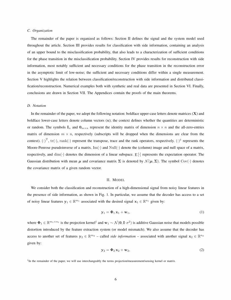
We consider both the classification and reconstruction of a high-dimensional signal from noisy linear features in

the presence of side information, as shown in Fig. 1. In particular, we assume that the decoder has access to a set

of noisy linear features y1 ∈ Rm1 associated with the desired signal x1 ∈ Rn1 given by:

y1 = Φ1 x1 + w1, (1)

where Φ1 ∈ Rm1×n1 is the projection kernel1 and w1 ∼ N (0, I·σ2) is additive Gaussian noise that models possible

distortion introduced by the feature extraction system (or model mismatch). We also assume that the decoder has

access to another set of features y2 ∈ Rm2 – called side information – associated with another signal x2 ∈ Rn2

given by:

y2 = Φ2 x2 + w2, (2)

1In the remainder of the paper, we will use interchangeably the terms projection/measurement/sensing kernel or matrix.

6

C1

x1Φ1 +

y1classifier / estimator C1 / x1

w1 ∼ N (0, I · σ2)

C2

x2Φ2 +

y2

side information

w2 ∼ N (0, I · σ2)

Fig. 1. Classification and reconstruction with side information. The user attempts to generate an estimate C1 of the index of the componentfrom which the input signal x1 was drawn (classification) or it aims to generate an estimate x1 of the input signal itself (reconstruction) onthe basis of the observation of both feature vectors y1 and y2.

where Φ2 ∈ Rm2×n2 is the projection kernel associated with the side information and w2 ∼ N (0, I·σ2) is Gaussian

additive noise, which is assumed to have the same covariance as the noise w1, for simplicity2. For the sake of

compact notation, we often re-write the models in (1) and (2) as:

y = Φ x + w, (3)

where

x =

x1

x2

, y =

y1

y2

, w =

w1

w2

(4)

and

Φ =

Φ1 0

0 Φ2

. (5)

We focus on random projection kernels, where both matrices Φ1 and Φ2 are assumed to be drawn from left

rotation-invariant distributions3.

We consider underlying class labels C1 ∈ {1, . . . ,K1} and C2 ∈ {1, . . . ,K2}, where C1 is associated with the

signal of interest x1 and C2 is associated with the side information signal x2. We assume that x1 and x2, conditioned

on the underlying class labels C1 = i and C2 = k, are drawn from a joint distribution p(x1,x2|C1 = i, C2 = k),

with the class labels drawn from probability pC1,C2(i, k). We assume that the decoder, for both classification and

reconstruction purposes, knows perfectly the joint probability mass function (pmf) pC1,C2(i, k) of the discrete

random variables corresponding to the class labels of x1 and x2, and the conditional distributions p(x1,x2|C1 =

i, C2 = k). For the problem of classification with side information, the objective is to estimate the value of the

2This assumption carries no loss of generality, because the following analysis holds even if we rescale y2 by a factor equal to the ratio betweenthe noise variances associated with w1 and w2.

3A random matrix A ∈ Rm×n is said to be (left or right) rotation-invariant if the joint probability density function (pdf) of its entries p(A)satisfies p(ΘA) = p(A), or p(AΨ) = p(A), respectively, for any orthogonal matrix Θ or Ψ. A special case of (left and right) rotation-invariant random matrices is represented by matrices with independent identically distributed (i.i.d.), zero-mean Gaussian entries with fixedvariance.

7

index C1 that identifies the distribution/component from which x1 was drawn, on the basis of the observation of

both vectors y1 and y2. The minimum average error probability in classifying C1 from y1 and y2 is achieved by

the maximum a posteriori (MAP) classifier [1], given by

C1 = arg maxi∈{1,...,K1}

p(C1 = i|y1,y2) (6)

= arg maxi∈{1,...,K1}

K2∑k=1

pC1,C2(i, k)p(y1,y2|C1 = i, C2 = k), (7)

where p(C1 = i|y1,y2) is the a posteriori probability of class C1 = i conditioned on y1 and y2.

For the problem of reconstruction with side information, the objective of the decoder is to estimate the signal

x1 from the observation of y1 and y2. In particular, we consider reconstruction obtained via the conditional mean

estimator

x1(y1,y2) = E [x1|y1,y2] =

∫x1p(x1|y1,y2)dx1, (8)

where p(x1|y1,y2) is the posterior pdf of x1 given the observations y1 and y2, which minimizes the reconstruction

error.

We emphasize the key distinction between the previously studied problems of distributed [50], [51] or multi-task

compressive sensing [57]: our goal is to recover x1 or its label C1, based upon compressive y1 and y2, while

previous work considered joint recovery of x1 and x2 (or joint estimation of C1 and C2). Note that our theory

allows the special case for which Φ2 is the identity matrix, in which case y2 = x2 and the side information is not

measured compressively. In addition, and more closely connected to previous work, we will consider the objectives

of jointly determining the pair of index values (C1, C2) that identify the distributions/components4 from which x1

and x2 were drawn, in the case of classification, and to estimate jointly x1 and x2, in the case of reconstruction.

The solution to these latter problems follows immediately from the solution to the side information problems.

Moreover, as is evident from (3), the distributed classification and reconstruction problem can be mapped into a

standard classification or reconstruction problem of a single signal, in which we are forcing the sensing matrix to

obey a block diagonal structure.

A. Signal, Side Information and Correlation Models

The key aspect now relates to the definition of the signal, side information, and the respective correlation models.

In particular, we adopt a multivariate Gaussian model for the distribution of x1 and x2, conditioned on (C1, C2) =

(i, k), i.e.

p(x1,x2|C1 = i, C2 = k) = N (µ(ik)x ,Σ(ik)

x ), (9)

4In the remainder of the paper we will also call C1 and C2 the classes associated to the input and side information signals, respectively.

8

where

µ(ik)x =

µ(ik)x1

µ(ik)x2

, Σ(ik)x =

Σ(ik)x1 Σ

(ik)x12

Σ(ik)x21 Σ

(ik)x2

, (10)

so that p(x1|C1 = i, C2 = k) = N (µ(ik)x1 ,Σ

(ik)x1 ) and p(x2|C1 = i, C2 = k) = N (µ

(ik)x2 ,Σ

(ik)x2 ), where µ

(ik)x1 and

Σ(ik)x1 are the mean and covariance matrix of x1 conditioned on the pair of classes (i, k), respectively, µ(ik)

x2 and

Σ(ik)x2 are the mean and covariance matrix of x2 conditioned on the pair of classes (i, k), respectively, and Σ

(ik)x12 is

the cross-covariance matrix between x1 and x2 conditioned on the pair of classes (i, k).

The motivation for this choice is associated by the fact that this apparently simple model can accommodate a

wide range of signal distributions. In fact, note that the joint pdf of x1 and x2 follows a GMM model:

p(x1,x2) =

K1∑i=1

K2∑k=1

pC1,C2(i, k)p(x1,x2|C1 = i, C2 = k), (11)

so that we can in principle approximate very complex distributions by incorporating additional terms in the

decomposition [59]. Note also that the conditional marginal pdfs of x1 and x2 also follow GMM models:

p(x1|C1 = i) =

K2∑k=1

pC2|C1(k|i)

∫dx2p(x1,x2|C1 = i, C2 = k) (12)

=

K2∑k=1

pC2|C1(k|i) N (µ(ik)

x1,Σ(ik)

x1) (13)

and

p(x2|C2 = k) =

K1∑i=1

pC1|C2(i|k)

∫dx1p(x1,x2|C1 = i, C2 = k) (14)

=

K1∑i=1

pC1|C2(i|k) N (µ(ik)

x2,Σ(ik)

x2), (15)

where pC2|C1(k|i) =

pC1,C2(i,k)

pC1(i) and pC1|C2

(i|k) =pC1,C2

(i,k)

pC2(k) are the conditional pmfs of C2 and C1. Therefore,

our model naturally subsumes the standard GMM models used in the literature to deliver state-of-the-art results in

reconstruction and classification problems, hyperspectral imaging and digit recognition applications [6].

We also adopt a framework that allows common and innovative components in the representation of x1 and x2

conditioned on (C1, C2) = (i, k), generalizing the one in [50], [51]. In particular, note that

p(x1,x2|C1 = i, C2 = k) = N (µ(ik)x ,Σ(ik)

x ) (16)

is equivalent to expressing x1 and x2 conditioned on the pair of classes (i, k) as

x1 = xc1 + x′1 + µ(ik)x1

= P(ik)c1 zc + P

(ik)1 z1 + µ(ik)

x1(17)

x2 = xc2 + x′2 + µ(ik)x2

= P(ik)c2 zc + P

(ik)2 z2 + µ(ik)

x2(18)

for an appropriate choice of the matrices P(ik)c1 ∈ Rn1×s(ik)

c ,P(ik)c2 ∈ Rn2×s(ik)

c ,P(ik)1 ∈ Rn1×s(ik)

1 ,P(ik)2 ∈ Rn2×s(ik)

2

9

and where the vectors zc ∼ N (0, Is(ik)c

), z1 ∼ N (0, Is(ik)1

) and z2 ∼ N (0, Is(ik)2

) are independent. Note that (17)

and (18) correspond to a factor or union-of-subspace model; the vector zc characterizes a shared latent process,

and P(ik)c1 and P

(ik)c2 are linear subspaces (dictionaries) that are a function of the properties of the signal and

side information, respectively. The vectors z1 and z2 are distinct latent processes, associated with respective linear

subspaces P(ik)1 and P

(ik)2 . So the model may be viewed from the perspective of generalizing previous union-of-

subspaces models [32]–[35].

In our scenario, the covariance matrix of x1 and x2 conditioned on the pair of classes (i, k) can be also written

as Σ(ik)x = P(ik)(P(ik))T, with

P(ik) =

P(ik)c1 P

(ik)1 0

P(ik)c2 0 P

(ik)2

, (19)

where P(ik)c1 ,P

(ik)c2 ,P

(ik)1 and P

(ik)2 are such that 5

Σ(ik)x1

= P(ik)c1 (P(ik)

c1 )T +P(ik)1 (P

(ik)1 )T , Σ(ik)

x2= P(ik)

c2 (P(ik)c2 )T +P

(ik)2 (P

(ik)2 )T , Σ(ik)

x12= P(ik)

c1 (P(ik)c2 )T.

(20)

We refer to the vectors xc1 ∼ N (0,Pc1(P(ik)c1 )T) and xc2 ∼ N (0,Pc2(P

(ik)c2 )T) as the common components:

these components of x1 and x2 are correlated, as they are obtained as linear combinations of atoms in two different

dictionaries (the columns of P(ik)c1 and P

(ik)c2 , respectively) but with the same weights, that are contained in the vector

zc, and therefore can be seen to model some underlying phenomena common to both x1 and x2 (conditioned on the

classes). On the other hand, we refer to x′1 ∼ N (0,P(ik)1 (P

(ik)1 )T) and x′2 ∼ N (0,P

(ik)2 (P

(ik)2 )T) as innovation

components: these components are statistically independent and thus can be seen to model phenomena specific to

x1 and x2 (conditioned on the classes).6

Therefore, we can now express the ranks of the matrices appearing in the model in (10) as a function of ranks

of the matrices appearing in the models in (17) and (18) as follows:

r(ik)x1= rank(Σ(ik)

x1) = rank[P(ik)

c1 P(ik)1 ] (21)

which represents the dimension of the subspace spanned by input signals x1 drawn from the Gaussian distribution

5Note that the common and innovation component representation proposed here is redundant, i.e., there are various choices of matricesP

(ik)c1 ,P

(ik)c2 ,P

(ik)1 ,P

(ik)2 that satisfy (20). We also emphasize that the results obtained in the following analysis hold irrespective of the

particular choice of the matrices P(ik)c1 ,P

(ik)c2 ,P

(ik)1 ,P

(ik)2 that satisfy (20). Then, although the adoption of the common and innovation

component representation is not required to prove the results contained in this work, we leverage such representation in order to give a clearinterpretation of the interaction between x1 and x2 and to underline the connection of our work with previous results in the literature.

6 The representation in (17) and (18) is reminiscent of the joint sparsity models JSM-1 and JSM-3 in [50], where signals sensed by multiplesensors were also described in terms of the sum of a common component plus innovation components. However, fundamental differencescharacterize our formulation with respect to such models: i) we consider a Bayesian framework in which the input signal and side informationsignal are picked from a mixture of components, where each component is described by a GMM distribution, whereas in JSM-1 and JSM-3all the components are deterministic; ii) in our model, the common components are correlated, but they are not exactly the same for x1 andx2, as it is instead for signals in JSM-1 and JSM-3; iii) in our case, the common and innovation components can be sparse over four differentbases, corresponding to the ranges of the matrices P

(ik)c1 ,P

(ik)c2 ,P

(ik)1 and P

(ik)2 ; on the other hand, all signals in JSM-1 and JSM-3 are

assumed to be sparse over the same basis.

10

corresponding to the indices C1 = i, C2 = k;

r(ik)x2= rank(Σ(ik)

x2) = rank[P(ik)

c2 P(ik)2 ] (22)

which represents the dimension of the subspace spanned by side information signals x2 drawn from the Gaussian

distribution corresponding to the indices C1 = i, C2 = k;

r(ik,j`)x1= rank(Σ(ik)

x1+ Σ(j`)

x1) = rank[P(ik)

c1 P(j`)c1 P

(ik)1 P

(j`)1 ] (23)

which represents the dimension of the sum of the subspaces spanned by input signals drawn from the Gaussian

distribution corresponding to the indices C1 = i, C2 = k and those from the Gaussian distribution corresponding

to the indices C1 = j, C2 = `;

r(ik,j`)x2= rank(Σ(ik)

x2+ Σ(j`)

x2) = rank[P(ik)

c2 P(j`)c2 P

(ik)2 P

(j`)2 ] (24)

which represents the dimension of the sum of the subspaces spanned by side information signals drawn from

the Gaussian distribution corresponding to the indices C1 = i, C2 = k and those from the Gaussian distribution

corresponding to the indices C1 = j, C2 = `; and finally, the corresponding dimensions spanned collectively by

input and side information signals are given by

r(ik)x = rank(Σ(ik)x ) = rank

P(ik)c1 P

(ik)1 0

P(ik)c2 0 P

(ik)2

(25)

r(ik,j`)x = rank(Σ(ik)x + Σ(j`)

x ) = rank

P(ik,j`)c1 P

(ik,j`)1 0

P(ik,j`)c2 0 P

(ik,j`)2

, (26)

where we have introduced the compact notation P(ik,j`)c1 = [P

(ik)c1 P

(j`)c1 ], P

(ik,j`)c2 = [P

(ik)c2 P

(j`)c2 ], P

(ik,j`)1 =

[P(ik)1 P

(j`)1 ] and P

(ik,j`)2 = [P

(ik)2 P

(j`)2 ].

We also define the rank:

r(ik) = rank(ΦΣ(ik)

x ΦT), (27)

that represents the dimension of the subspace in Rm1+m2 spanned collectively by the projections of input signals

and the projections of side information signals drawn from the Gaussian distribution identified by the component

indices C1 = i, C2 = k, and

r(ik,j`) = rank(Φ(Σ(ik)

x + Σ(j`)x )ΦT

), (28)

that represents the dimension of the subspace obtained by summing the subspace in Rm1+m2 spanned collectively by

the projections of input signals and the projections of side information signals drawn from the Gaussian distribution

identified by the component indices C1 = i, C2 = k with the subspace spanned by the projections of input signals

and the projections of side information signals drawn from the Gaussian distribution identified by the component

indices C1 = j, C2 = `.

11

The quantities in (21)–(28), which provide a concise description of the geometry of the input source, the side

information source, and the geometry of the interaction of such sources with the projections kernels, will be

fundamental to determining the performance of the classification and reconstruction of high-dimensional signals

from low-dimensional features in the presence of side information.

III. CLASSIFICATION WITH SIDE INFORMATION

We first consider signal classification in the presence of side information. The basis of the analysis is an asymptotic

characterization – in the limit of σ2 → 0 – of the behavior of an upper bound to the misclassification probability

associated with the optimal MAP classifier (rather than the exact misclassification probability which is not tractable).

In particular, for a two class problem7, i.e., when K1 = 2, via the Bhattacharyya bound [1], the misclassification

probability can be upper bounded as follows:

Perr =√pC1(1)pC1(2)

∫ √p(y|C1 = 1)p(y|C1 = 2)dy (29)

=√pC1

(1)pC1(2)

∫ √√√√ K2∑k.`=1

pC2|C1(k|1)pC2|C1

(`|2)p(y|C1 = 1, C2 = k)p(y|C1 = 2, C2 = `)dy. (30)

For a multiple class problem, via the Bhattacharyya bound in conjunction with the union bound, the misclassification

probability can be upper bounded as follows:

Perr =

K1∑i=1

K1∑j=1j 6=i

pC1(i)

∫ √√√√ K2∑k.`=1

pC2|C1(k|i)pC2|C1

(`|j)p(y|C1 = i, C2 = k)p(y|C1 = j, C2 = `)dy. (31)

The asymptotic characterization that we discuss below – akin to that in [67] – is based on two key metrics. The

first one identifies the presence or absence of an error floor in the upper bound to the misclassification probability

as σ2 → 0, leading to conditions on the number of features that guarantee perfect classification in the low-noise

regime, i.e.,

limσ2→0

Perr(σ2) = 0. (32)

Note that the characterization of the presence or absence of an error floor in the upper bound of the misclassification

probability also leads to the characterization of a phase transition region in terms of m1 and m2, where within

this region limσ2→0 Perr(σ2) = 0 and outside the region limσ2→0 Perr(σ

2) > 0. Note also that the boundaries of

the region associated to the upper bound of the misclassification probability represent also lower bounds of the

boundaries of the corresponding region associated with the true error probability.

The second metric offers a more refined description of the behavior of the upper bound to the misclassification

probability by considering the slope at which log Perr decays (in a log σ2 scale) in the low-noise regime. Such

7The number of classes corresponding to the side information signal, K2, can be arbitrary.

12

value is named the diversity-order and is given by

d = limσ2→0

log Perr(σ2)

log σ2. (33)

Note also that the diversity-order associated with the upper bound of the error probability represents a lower bound

on (the absolute value of) the slope of the true error probability in the low-noise regime.

We next characterize these quantities as a function of the number of features/measurements m1 and m2 and as

a function of the underlying geometry of the signal and the side information, both for zero-mean classes (signal

lives in a union of linear subspaces) and nonzero-mean ones (signal lives in a union of affine spaces). We also

characterize the quantities in (32) and (33) in terms of the diversity-order associated with the classification of two

Gaussian distributions N (µ(ik)x ,Σ

(ik)x ) and N (µ

(j`)x ,Σ

(j`)x ) from the observation of the noisy linear features y in

(3),

d(ik, j`) = limσ2→0

1

log σ2log

(√pC1,C2

(i, k)pC1,C2(j, `)

∫ √p(y|C1 = i, C2 = k)p(y|C1 = j, C2 = `)dy

).

(34)

Moreover, all the pairs of indices (i, k) such that pC1,C2(i, k) = 0 clearly do not affect the diversity-order associated

to classification with side information. Therefore, we can define the set of index pairs of interest as

S = {(i, k) ∈ {1, . . . ,K1} × {1, . . . ,K2} : pC1,C2(i, k) > 0} . (35)

We also define the set of index quadruples

SSIC = {(i, k, j, `) : (i, k), (j, `) ∈ S, i 6= j}, (36)

that play a key role in the computation of the diversity-order associated to classification with side information.

A. Zero-Mean Classes

We now provide a low-noise expansion of the upper bound to the misclassification probability associated with

the system with side information in (1) and (2), when assuming that the signals involved are all zero-mean, i.e.,

µ(ik)x = 0,∀(i, k).

Theorem 1: Consider the model in (1) and (2), where the input signal x1 is drawn according to the class-

conditioned distribution (13), the side information x2 is drawn according to the class-conditioned distribution (15),

and the class-conditioned joint distribution of x1 and x2 is given by (9) with µ(ik)x = 0,∀(i, k). Then, with

probability 1, in the low-noise regime, i.e., when σ2 → 0, the upper bound to the misclassification probability (31)

can be expanded as

Perr(σ2) = A · (σ2)d + o

((σ2)d

), (37)

for a fixed constant A > 0, where

d = min(i,k,j,`)∈SSIC

d(ik, j`), (38)

13

with

d(ik, j`) =1

2

(r(ik,j`) − r(ik) + r(j`)

2

), (39)

and

r(ik,j`) = rank(Φ(Σ(ik)

x + Σ(j`)x )ΦT

)(40)

= min{r(ik,j`)x ,min{m1, r(ik,j`)x1

}+ min{m2, r(ik,j`)x2

}}, (41)


x ΦT)

(42)

= min{r(ik)x ,min{m1, r(ik)x1}+ min{m2, r

(ik)x2}} (43)

and r(j`) is obtained as r(ik).

Proof: See Appendix A.

Theorem 1 provides a complete characterization of the slope of the upper bound to the misclassification probability

for the case of zero-mean classes, in terms of the number of features and the geometrical description of the sources.

In particular, observe that:

• The diversity-order d associated with the estimation of the component index C1 from noisy linear features with

side information is given by the worst-case diversity-order term d(ik, j`) associated with pair-wise classification

problems for which the indices corresponding to C1 are not the same (i 6= j).

• The diversity-order in (38), which depends on the pairwise diversity-order in (39), can also be seen to depend

on the difference between the dimension of the sum of the linear spaces collectively spanned by signals Φ1x1

and Φ2x2 drawn from the Gaussian distributions with indices (i, k) and (j, `) and the dimension of those

spaces taken individually. This dependence in the presence of side information is akin to that in the absence

of side information: the additional information, however, provides subspaces with increased dimensions over

which it is possible to discriminate among signals belonging to different classes.

• The effect of the correlation between x1 and x2 is embodied in the rank expressions (41) and (43). In

particular, we note that, in case x1 and x2 are conditionally independent given any pairs of classes (C1, C2),

i.e., p(x1,x2|C1 = i, C2 = k) = p(x1|C1 = i, C2 = k)p(x2|C1 = i, C2 = k), then r(ik)x = r(ik)x1 +r

(ik)x2 , r(j`)x =

r(j`)x1 +r

(j`)x2 and r(ik,j`)x = r

(ik,j`)x1 +r

(ik,j`)x2 . Then, the diversity-order is given by the sum of the diversity-order

values corresponding to the classification of x1 from y1 and that corresponding to the classification of x2 from

y2. From a geometrical point of view, when x1 and x2 are conditionally independent, the linear spaces spanned

by the side information offer new dimensions over which the decoder can discriminate among classes, which

are completely decoupled from the dimensions corresponding to linear spaces spanned by the realizations of

x1. Otherwise, when x1 and x2 are not conditionally independent, the diversity-order can be in general larger

than, smaller than, or equal to the sum of the diversity-order values corresponding to the classification of x1

from y1 and that corresponding to the classification of x2 from y2.

14

A direct consequence of the asymptotic characterization of the upper bound to the misclassification probability

in (31) is access to conditions on the number of features m1 and m2 that are both necessary and sufficient to drive

the upper bound to the misclassification probability to zero when σ2 → 0, that is, in order to achieve the phase

transition of the upper bound to the misclassification probability, and hence a condition on the number of features

m1 and m2 that is sufficient to drive the true misclassification probability to zero when σ2 → 0.

Corollary 1: Consider the model in (1) and (2), where the input signal x1 is drawn according to the class-


and the class-conditioned joint distribution of x1 and x2 is given by (9) with µ(ik)x = 0,∀(i, k).

If there exists an index quadruple (i, k, j, `) ∈ SSIC such that r(ik,j`)x = r(ik)x = r

(j`)x , then, d = 0 and the

upper bound to the misclassification probability (31) exhibits an error floor in the low-noise regime. Otherwise,

if r(ik,j`)x > r(ik)x , r

(j`)x , ∀(i, k, j, `) ∈ SSIC, then, with probability 1, the upper bound to the misclassification

probability (31) approaches zero when σ2 → 0 if and only if the following conditions hold ∀(i, k, j, `) ∈ SSIC:

1) if r(ik,j`)x1 > r(ik)x1 , r

(j`)x1 and r(ik,j`)x2 > r

(ik)x2 , r

(j`)x2 :

m1 > min{r(ik)x1, r(j`)x1

} or m2 > min{r(ik)x2, r(j`)x2

} or m1 +m2 > min{r(ik)x , r(j`)x }; (44)

2) if r(ik,j`)x1 = r(ik)x1 = r

(j`)x1 and r(ik,j`)x2 = r

(ik)x2 = r

(j`)x2 :

m1 > min{r(ik)x − r(ik)x2 , r(j`)x − r(j`)x2 }


m1 +m2 > min{r(ik)x , r(j`)x }

; (45)

3) if r(ik,j`)x1 > r(ik)x1 , r


(ik)x2 = r

(j`)x2 :


} or



; (46)

4) if r(ik,j`)x1 = r(ik)x1 = r


(ik)x2 , r

(j`)x2 :


} or



. (47)

Proof: See Appendix B.

The characterization of the numbers of features m1 and m2 that are both necessary and sufficient to achieve the

phase transition in the upper bound to the misclassification probability is divided in 4 cases, depending on whether

the range spaces Im(Σ(ik)x1 ) and Im(Σ

(j`)x1 ), or the range spaces Im(Σ

(ik)x2 ) and Im(Σ

(j`)x2 ), are distinct or not8.

Fig. 2 depicts the tradeoff between the values of m1 and m2 associated with these different cases. Note also that

the values of m1 and m2 associated with the phase transition of the upper bound of the misclassification probability

8We recall that, given two positive semidefinite matrices A and B with ranks rA = rank(A), rB = rank(B), rAB = rank(A + B),Im(A) = Im(B) if and only if rAB = rA+rB

2[64, Lemma 2] and then, if and only if rAB = rA = rB.

15

m2

m1b1

b2

m1 +m

2 =c

(a)

m2

m1b1a1

a2

b2

(b)

m2

m1b1a1

a2

b2

(c)

m2

m1b1a1

a2

b2

(d)

Fig. 2. Representation of the conditions on m1 and m2 for phase transition, for the 4 different cases encapsulated in Corollary 1. In all casesa1 = min{r(ik)x −r(ik)x2

, r(j`)x −r(j`)x2

}+1, b1 = min{r(ik)x1, r

(j`)x1}+1, a2 = min{r(ik)x −r(ik)x1

, r(j`)x −r(j`)x2

}+1, b2 = min{r(ik)x2, r

(j`)x2}+1

and c = min{r(ik)x , r(j`)x }+ 1. The shaded regions represent values of m1 and m2 that satisfy the conditions (44)–(47).

lie in the intersection of the regions corresponding to index quadruples (i, k, j, `) ∈ SSIC.

In case 1), the range spaces associated to the input covariance matrices are all distinct, and by observing (44) we

can clearly determine the beneficial effect of the correlation between x1 and x2 in guaranteeing the phase transition

for the upper bound to the misclassification probability. Namely, we note that the phase transition is achieved

either when error-free classification is possible from the observation of y1 alone (m1 > min{r(ik)x1 , r(j`)x1 }) or from

the observation of y2 alone (m2 > min{r(ik)x2 , r(j`)x2 }) cf. [67], but, more importantly, the condition m1 + m2 >

min{r(ik)x , r(j`)x } shows the benefit of side information in order to obtain the phase transition with a lower number

of features. In fact, when r(ik)x < r(ik)x1 + r

(ik)x2 , joint classification of y1 and y2 leads to a clear advantage in the

number of features needed to achieve the phase transition with respect to the case in which classification is carried

independently from y1 and y2, despite the fact that linear features are extracted independently from x1 and x2.

In case 2), the range spaces associated to the input covariance matrices are such that Im(Σ(ik)x1 ) = Im(Σ

(j`)x1 ) and

Im(Σ(ik)x2 ) = Im(Σ

(j`)x2 ) so that classification based on the observation of y1 or y2 alone yields an error floor in

the upper bound of the misclassification probability [67]. In other terms, input signals and side information signals

from classes (i, k) and (j, `) are never perfectly distinguishable. In this case, the impact of correlation between

the input signal and the side information signal is clear when observing (45). In fact, when combining features

extracted independently from the vectors x1 and x2, it is possible to drive to zero the misclassification probability,

in the low-noise regime, provided that the number of features extracted m1 and m2 verify the conditions in (45).

Finally, cases 3) and 4) represent intermediate scenarios in which range spaces associated to x1 are distinct,

but those related to x2 are completely overlapping, and vice versa. We note then how the necessary and sufficient

conditions for phase transition in (46) and (47) are given by combinations of the conditions in (44) and (45).

We further note in passing that the conditions in (45) are reminiscent of the conditions on compression rates for

lossless joint source coding in [40].

16

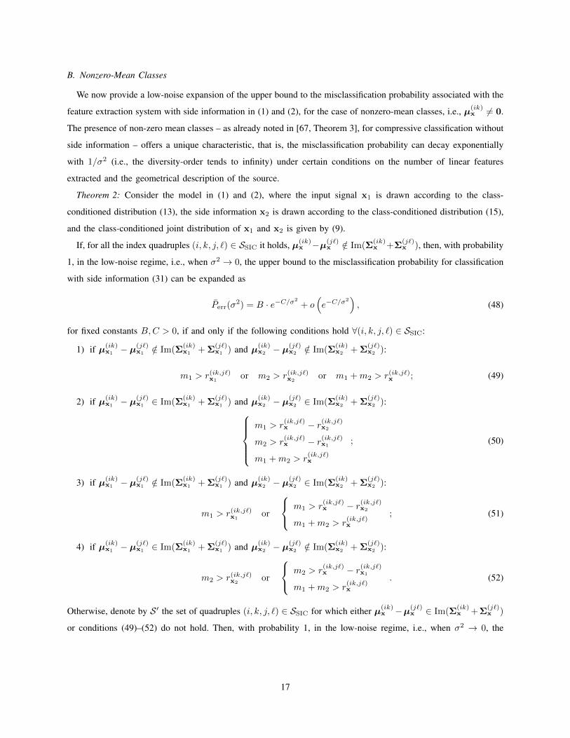
B. Nonzero-Mean Classes

We now provide a low-noise expansion of the upper bound to the misclassification probability associated with the

feature extraction system with side information in (1) and (2), for the case of nonzero-mean classes, i.e., µ(ik)x 6= 0.

The presence of non-zero mean classes – as already noted in [67, Theorem 3], for compressive classification without

side information – offers a unique characteristic, that is, the misclassification probability can decay exponentially

with 1/σ2 (i.e., the diversity-order tends to infinity) under certain conditions on the number of linear features

extracted and the geometrical description of the source.

Theorem 2: Consider the model in (1) and (2), where the input signal x1 is drawn according to the class-


and the class-conditioned joint distribution of x1 and x2 is given by (9).

If, for all the index quadruples (i, k, j, `) ∈ SSIC it holds, µ(ik)x −µ(j`)

x /∈ Im(Σ(ik)x +Σ

(j`)x ), then, with probability

1, in the low-noise regime, i.e., when σ2 → 0, the upper bound to the misclassification probability for classification

with side information (31) can be expanded as

Perr(σ2) = B · e−C/σ

2

+ o(e−C/σ

2), (48)

for fixed constants B,C > 0, if and only if the following conditions hold ∀(i, k, j, `) ∈ SSIC:

1) if µ(ik)x1 − µ

(j`)x1 /∈ Im(Σ

(ik)x1 + Σ

(j`)x1 ) and µ

(ik)x2 − µ

(j`)x2 /∈ Im(Σ

(ik)x2 + Σ

(j`)x2 ):

m1 > r(ik,j`)x1or m2 > r(ik,j`)x2

or m1 +m2 > r(ik,j`)x ; (49)


(j`)x1 ∈ Im(Σ

(ik)x1 + Σ

(j`)x1 ) and µ

(ik)x2 − µ

(j`)x2 ∈ Im(Σ

(ik)x2 + Σ

(j`)x2 ):

m1 > r(ik,j`)x − r(ik,j`)x2


m1 +m2 > r(ik,j`)x

; (50)


(j`)x1 /∈ Im(Σ

(ik)x1 + Σ

(j`)x1 ) and µ

(ik)x2 − µ

(j`)x2 ∈ Im(Σ

(ik)x2 + Σ

(j`)x2 ):

m1 > r(ik,j`)x1or


m1 +m2 > r(ik,j`)x

; (51)


(j`)x1 ∈ Im(Σ

(ik)x1 + Σ

(j`)x1 ) and µ

(ik)x2 − µ

(j`)x2 /∈ Im(Σ

(ik)x2 + Σ

(j`)x2 ):

m2 > r(ik,j`)x2or


m1 +m2 > r(ik,j`)x

. (52)

Otherwise, denote by S ′ the set of quadruples (i, k, j, `) ∈ SSIC for which either µ(ik)x −µ

(j`)x ∈ Im(Σ

(ik)x +Σ

(j`)x )

or conditions (49)–(52) do not hold. Then, with probability 1, in the low-noise regime, i.e., when σ2 → 0, the

17

upper bound to the misclassification probability for classification with side information (31) can be expanded as

Perr(σ2) = A · (σ2)d + o

((σ2)d

), (53)

for a fixed constant A > 0, and

d = min(i,k,j,`)∈S′

d(ik, j`), (54)

where d(ik, j`) is obtained as in Theorem 1.

Proof: See Appendix C.

Note that classification based on the joint observation of y1 and y2 can guarantee infinite diversity-order even

when classification based on y1 or y2 alone cannot. In particular, if there exists an index quadruple for which both

µ(ik)x1 − µ

(j`)x1 ∈ Im(Σ

(ik)x1 + Σ

(j`)x1 ) and µ

(ik)x2 − µ

(j`)x2 ∈ Im(Σ

(ik)x2 + Σ

(j`)x2 ), then, irrespective of the number of

features m1 and m2 and of the specific values of the projection kernels Φ1 and Φ2, we have

Φ1(µ(ik)x1− µ(j`)

x1) ∈ Im(Φ1(Σ(ik)

x1+ Σ(j`)

x1)ΦT

1 ) , Φ2(µ(ik)x2− µ(j`)

x2) ∈ Im(Φ2(Σ(ik)

x2+ Σ(j`)

x2)ΦT

2 ) (55)

and, therefore, the conditions in [67, Theorem 3] are not verified, thus implying that both the upper bounds to

the error probability associated to classification based on y1 or y2 do not decay exponentially with 1/σ2 when

σ2 → 0. On the other hand, if µ(ik)x − µ

(j`)x /∈ Im(Σ

(ik)x + Σ

(j`)x ) for all index quadruples (i, k, j, `) ∈ SSIC,

then classification based on both y1 and y2 is characterized by an exponential decay of the upper bound to the

misclassification probability, provided that conditions (49)–(52) on the numbers of features extracted from x1 and

x2 are verified.

Moreover, the conditions on the number of features needed to achieve an exponential decay in 1/σ2 of the upper

bound to the misclassification probability depend on whether the affine spaces spanned by signal and side information

realization in the Gaussian classes (i, k) and (j, `) do intersect or not, for all index quadruples (i, k, j, `) ∈ SSIC.

From a geometrical point of view, if the affine spaces spanned by the overall signal x obtained by the concatenation

of input signal and side information do not intersect, then equations (49)–(52) determine conditions on the number

of extracted features m1 and m2 such that the affine spaces spanned by the projected signals Φx do not intersect

as well, thus guaranteeing enhanced discrimination among classes.

IV. RECONSTRUCTION WITH SIDE INFORMATION

We now consider signal reconstruction in the presence of side information. We are interested in the asymptotic

characterization of the minimum mean-squared error (MMSE) incurred in reconstructing x1 from the observation

of the signal features y1 and the side information features y2, given by9

MMSE1|1,2(σ2) = E[‖x1 − x1(y1,y2)‖2

], (56)

9We emphasize that MMSE1|1,2(σ2) is a function of σ2.

18

where x1(y1,y2) is the conditional mean estimator in (8). In particular, we are interested in determining conditions

on the number of linear features m1 and m2 that guarantee perfect reconstruction in the low-noise regime, i.e.,

when σ2 → 0, that is

limσ2→0

MMSE1|1,2(σ2) = 0, (57)

thus generalizing the results in [64] to the case when side information is available at the decoder; the misclassification

results will be key to address this problem.

Note the characterization of such conditions also leads to the characterization of a phase transition region in terms

of m1 and m2, where within this region limσ2→0 MMSE1|1,2(σ2) = 0 and outside the region limσ2→0 MMSE1|1,2(σ2) >

0.

A. Preliminaries: Gaussian Sources

We first consider the simplified case in which K1 = K2 = 1, i.e., when the signals x1 and x2 obey the joint

Gaussian distribution N (µx,Σx), where

µx =

µx1

µx2

, Σx =

Σx1 Σx12

Σx21Σx2

, (58)

and with ranks rx1 = rank(Σx1), rx2 = rank(Σx2) and rx = rank(Σx).

For this case, the conditional mean estimator is given by [70]

x1(y) = µx1+ Wx1

(y −Φµx) , (59)

where

Wx1= [Σx1

Σx12] ΦT

(σ2I + ΦΣxΦT

)−1. (60)

Moreover, the MMSE in this case can be expressed as

MMSEG1|1,2(σ2) = tr

Σx1− [Σx1

Σx12] ΦT

(σ2I + ΦΣxΦT

)−1Φ

ΣTx1

ΣTx2

. (61)

In the following, we provide necessary and sufficient conditions on the number of features m1,m2 that guarantee

that, in the low-noise regime, the reconstruction MMSE for Gaussian sources approaches zero. Sufficient conditions

are based on the analysis of two different upper bounds to MMSEG(σ2). The first upper bound is obtained by

considering the MMSE associated with the reconstruction of the signal x1 from the observation of y1 alone, i.e.,

without side information, which is denoted by

MMSEG1|1(σ2) = E

[‖x1 − x1(y1)‖2

], (62)

where x1(y1) = E [x1|y1] and whose behavior in the low-noise regime has been analyzed in [64].

The second upper bound is obtained by considering the MMSE associated with the distributed reconstruction

19

problem, i.e., the joint recovery of x1 and x2 from the observation of both y1 and y2 (i.e., the reconstruction of

x from y), which is denoted by

MMSEG1,2|1,2(σ2) = E

[‖x− x(y)‖2

], (63)

where

x(y) = E [x|y] =

∫x p(x|y)dx. (64)

Note that the analysis of the second upper bound cannot be directly performed on the basis of the results in [64],

due to the particular block diagonal structure of Φ.

Based on the properties of the MMSE [70], it is straightforward to show that MMSEG1|1,2(σ2) ≤ MMSEG

1|1(σ2)

and MMSEG1|1,2(σ2) ≤ MMSEG

1,2|1,2(σ2).

On the other hand, necessary conditions are derived from the analysis of the lower bound to the MMSE obtained

by feeding the decoder not only with the noisy features y1 and y2, but also with the values of the realizations of the

noise vectors w1 and w2. The following theorem stems from the fact that the necessary and sufficient conditions

for the phase transition of the MMSE coincide.

Theorem 3: Consider the model in (1) and (2). Assume that the vectors x1,x2 are jointly Gaussian, with distribu-

tion N (µx,Σx), with mean and covariance matrix specified in (58), and with rx1= rank(Σx1

), rx2= rank(Σx2

)

and rx = rank(Σx). Then, with probability 1, we have

limσ2→0

MMSEG1|1,2(σ2) = 0⇔ m1 ≥ rx1

or

m1 ≥ rx − rx2

m1 +m2 ≥ rx. (65)

Proof: See Appendix D.

Without side information, it is known that m1 ≥ rx1 represents a necessary and sufficient condition on the

number of features needed to drive the MMSE to zero in the low-noise regime [64]. With side information, it is

possible to reliably recover the input signal x1 with a lower number of features, as described by the conditions in

(65). In fact, whenever rx < rx1 + rx2 , it is possible to perfectly reconstruct x1 when σ2 → 0 even with less than

rx1 features, provided that m1 +m2 ≥ rx. This happens when the dimension of the overall space spanned by the

projected signals obtained by concatenating the input signal and the side information signal, i.e., Φx, is greater

than or equal to the dimension of the space spanned by x in the signal domain. Moreover, the m1 features extracted

from x1 need to be enough to span a space with dimension equal to the difference between the dimension of the

space spanned by x and that spanned by x2 alone. In this sense, linear projections extracted from the input signal

must be enough to capture signal features that are characteristic of x1 and are not “shared” with x2, meaning that

they are not correlated.

The values of m1 and m2 that satisfy the necessary and sufficient conditions (65) are reported in Fig. 3.

20

m2

m1rx1rx − rx2

rx − rx1

rx2 m1 +m2 =

rx

Fig. 3. Representation of the conditions on m1 and m2 for phase transition of the MMSE for Gaussian sources. The shaded region representsvalues of m1 and m2 that satisfy the conditions (65).

B. GMM Sources

We now consider the more general case where the signals x1 and x2 follow the models in Section II-A. It

is possible to express the conditional mean estimator in closed form, but not the MMSE, which we denote by

MMSEGM1|1,2(σ2). Therefore, we will determine necessary and sufficient conditions on the numbers of features m1

and m2 that guarantee MMSEGM1|1,2(σ2)→ 0 in the low-noise regime, by leveraging the result in Theorem 3 together

with steps akin to those in [64, Section IV].

1) Sufficient Conditions: In order to provide sufficient conditions for the MMSE to approach zero in the low-

noise regime, we analyze the upper bound to the MMSE corresponding to the mean squared error (MSE) associated

with a (sub-optimal) classify and reconstruct decoder, which we denote by MSECR(σ2). This decoder operates in

two steps as follows:

• First, the decoder estimates the pair of class indices associated to the input signal and the side information

signal via the MAP classifier10

(C1, C2) = arg max(i,k)

p(y|C1 = i, C2 = k)pC1,C2(i, k); (66)

• Second, in view of the fact that, conditioned on (C1, C2) = (i, k), the vectors x1 and x2 are jointly Gaussian

distributed with mean µ(ik)x and covariance Σ

(ik)x , the decoder reconstructs the input signal x1 by using the

conditional mean estimator corresponding to the estimated classes C1, C2

x1(y;C1 = C1, C2 = C2) = µ(C1C2)x1

+ W(C1C2)x1

(y −Φµ(C1C2)

x

), (67)

10This MAP classifier is associated with the distributed classification problem, which will be shown to be closely related to the problem ofclassification with side information in the next section.

21

where

W(C1C2)x1

=[Σ(C1C2)

x1Σ(C1C2)

x12

]ΦT

(σ2I + ΦΣ(C1C2)

x ΦT)−1

. (68)

The optimality of the MMSE estimator immediately implies that MMSEGM1|1,2(σ2) ≤ MSECR(σ2). Therefore, we

can immediately leverage the analysis of the misclassification probability carried out in Section III and the result

in Theorem 3 in order to characterize the behavior of MSEGMCR(σ2) in the low-noise regime, in order to determine

sufficient condition for the phase transition of MMSEGM1|1,2(σ2).

Theorem 4: Consider the model in (1) and (2). Assume that the input signal x1 is drawn according to the

class-conditioned distribution (13), x2 is drawn according to the class-conditioned distribution (15) and the class-

conditioned joint distribution of x1 and x2 is given by (9). Then, with probability 1, we have

m1 > r(ik)x1or

m1 > r(ik)x − r(ik)x2

m1 +m2 > r(ik)x

,∀(i, k) ∈ S ⇒ limσ2→0

MMSEGM1|1,2(σ2) = 0. (69)

Proof: See Appendix E.

The sufficient conditions in (69) show that – akin to the Gaussian case – the numbers of features extracted

from x1 and x2 have to be collectively greater than the largest among the dimensions of the spaces spanned by

signals x = [xT1 xT

2 ]T in the Gaussian components corresponding to indices (C1, C2) = (i, k), for i = 1, . . . ,K1,

k = 1, . . . ,K2. Moreover, the features extracted from x1 need to be enough to capture signal components which

are not correlated with the side information, for all Gaussian components. Finally, the condition m1 > r(ik)x1 is

obtained trivially by considering reconstruction of x1 from the features collected in the vector y1, thus disregarding

side information.

Note that the values of m1 and m2 that are sufficient for the MMSE phase transition are obtained by considering

the intersection of regions akin to that in Fig. 3 for all the pairs of classes (i, k) ∈ S.

Appendix E shows that the conditions in (69) guarantee that the decoder can reliably estimate the class indices

(C1, C2) and hence reliably reconstruct the signal x1 in the low-noise regime.

2) Necessary conditions: We now derive necessary conditions for the phase transition of the MMSE of GMM

sources with side information. We obtain such conditions from the analysis of a lower bound to the MMSE that is

obtained by observing that

MMSEGM1|1,2(σ2) = E

[‖x1 − x1(y1,y2)‖2

](70)

=∑

(i,k)∈S

pC1,C2(i, k) E

[‖x1 − x1(y1,y2)‖2|C1 = i, C2 = k

](71)

≥∑

(i,k)∈S

pC1,C2(i, k)MMSEG(i,k)

1|1,2 (σ2) = MSELB(σ2), (72)

where MMSEG(i,k)1|1,2 (σ2) denotes the MMSE associated with the reconstruction of the Gaussian signal x1 corre-

sponding to class indexes (i, k) from the observation of the vector y1 and the side information y2. Note that the

equality in (71) is obtained via the total probability formula and the inequality in (72) is a consequence of the

22

optimality of the MMSE estimator for joint Gaussian input and side information signals.

The analysis of MSELB(σ2) leads to the derivation of the following necessary conditions on the number of

features m1 and m2 needed to drive MMSEGM1|1,2(σ2) to zero when σ2 → 0.




limσ2→0

MMSEGM1|1,2(σ2) = 0⇒ m1 ≥ r(ik)x1

or

m1 ≥ r(ik)x − r(ik)x2

m1 +m2 ≥ r(ik)x

,∀(i, k) ∈ S. (73)

Proof: The proof is based on the result in Theorem 3, which implies that, if MMSEG(i,k)1|1,2 (σ2) → 0 when

σ2 → 0, ∀(i, k) ∈ S, then, with probability 1, the conditions on the numbers of features m1 and m2 in (73) must

be satisfied for all (i, k) ∈ S.

It is interesting to note that the necessary conditions for the phase transition of the MMSE of GMM inputs are

one feature away from the corresponding sufficient conditions, akin to our previous results for the case without

side information [64]. In this way, Theorems 4 and 5 provide a sharp characterization of the region associated to

the phase transition of the MMSE of GMM inputs with side information.

V. DISTRIBUTED CLASSIFICATION AND RECONSTRUCTION

The problem of classification and reconstruction with side information are intimately related to the problems of

distributed classification and reconstruction, and our tools immediately generalize to provide insight about these

problems.

A. Distributed Classification

The problem of distributed classification involves the estimation of the pair of classes (C1, C2) from the low-

dimensional feature vectors y1 and y2, where

(C1, C2) = arg max(i,k)

p(y|C1 = i, C2 = k)pC1,C2(i, k); (74)

Via the Bhattacharyya bound and the union bound, it is possible to write an upper bound to the misclassification

probability of distributed classification as

Perr =∑

(i,k,j,`)∈SDC

pC1,C2(i, k)

∫ √p(y|C1 = i, C2 = k)p(y|C1 = j, C2 = `)dy, (75)

where

SDC = {(i, k, j, `) : (i, k), (j, `) ∈ S, (i, k) 6= (j, `)}, (76)

is a set corresponding to all couples of class index pairs that are different in at least one of the values for C1 or

C2. We can also explore the previous methodology to construct an asymptotic characterization of the upper bound

23

to the misclassification probability. We first consider the case of zero-mean classes, i.e., we assume µ(i,k)x = 0,

∀(i, k).

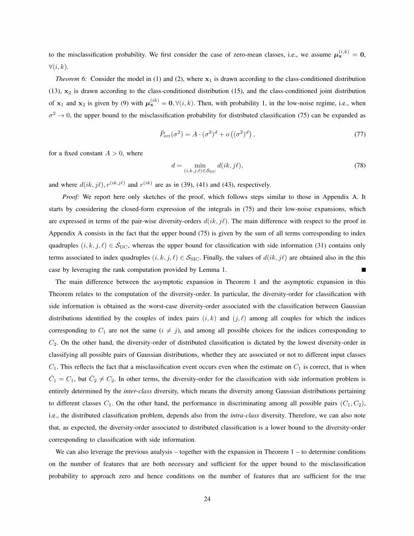
Theorem 6: Consider the model in (1) and (2), where x1 is drawn according to the class-conditioned distribution

(13), x2 is drawn according to the class-conditioned distribution (15), and the class-conditioned joint distribution

of x1 and x2 is given by (9) with µ(ik)x = 0,∀(i, k). Then, with probability 1, in the low-noise regime, i.e., when

σ2 → 0, the upper bound to the misclassification probability for distributed classification (75) can be expanded as

Perr(σ2) = A · (σ2)d + o

((σ2)d

), (77)

for a fixed constant A > 0, where

d = min(i,k,j,`)∈SDC

d(ik, j`), (78)

and where d(ik, j`), r(ik,j`) and r(ik) are as in (39), (41) and (43), respectively.

Proof: We report here only sketches of the proof, which follows steps similar to those in Appendix A. It

starts by considering the closed-form expression of the integrals in (75) and their low-noise expansions, which

are expressed in terms of the pair-wise diversity-orders d(ik, j`). The main difference with respect to the proof in

Appendix A consists in the fact that the upper bound (75) is given by the sum of all terms corresponding to index

quadruples (i, k, j, `) ∈ SDC, whereas the upper bound for classification with side information (31) contains only

terms associated to index quadruples (i, k, j, `) ∈ SSIC. Finally, the values of d(ik, j`) are obtained also in the this

case by leveraging the rank computation provided by Lemma 1.

The main difference between the asymptotic expansion in Theorem 1 and the asymptotic expansion in this

Theorem relates to the computation of the diversity-order. In particular, the diversity-order for classification with

side information is obtained as the worst-case diversity-order associated with the classification between Gaussian

distributions identified by the couples of index pairs (i, k) and (j, `) among all couples for which the indices

corresponding to C1 are not the same (i 6= j), and among all possible choices for the indices corresponding to

C2. On the other hand, the diversity-order of distributed classification is dictated by the lowest diversity-order in

classifying all possible pairs of Gaussian distributions, whether they are associated or not to different input classes

C1. This reflects the fact that a misclassification event occurs even when the estimate on C1 is correct, that is when

C1 = C1, but C2 6= C2. In other terms, the diversity-order for the classification with side information problem is

entirely determined by the inter-class diversity, which means the diversity among Gaussian distributions pertaining

to different classes C1. On the other hand, the performance in discriminating among all possible pairs (C1, C2),

i.e., the distributed classification problem, depends also from the intra-class diversity. Therefore, we can also note

that, as expected, the diversity-order associated to distributed classification is a lower bound to the diversity-order

corresponding to classification with side information.

We can also leverage the previous analysis – together with the expansion in Theorem 1 – to determine conditions

on the number of features that are both necessary and sufficient for the upper bound to the misclassification

probability to approach zero and hence conditions on the number of features that are sufficient for the true

24

misclassification probability to approach zero.

Corollary 2: Consider the model in (1) and (2), where x1 is drawn according to the class-conditioned distribution

(13), x2 is drawn according to the class-conditioned distribution (15), and the class-conditioned joint distribution

of x1 and x2 is given by (9) with µ(ik)x = 0,∀(i, k).

If there exists an index quadruple (i, k, j, `) ∈ SDC such that r(ik,j`)x = r(ik)x = r

(j`)x , then, d = 0 and the

upper bound to the misclassification probability for distributed classification (75) exhibits an error floor in the

low-noise regime. Otherwise, if r(ik,j`)x > r(ik)x , r

(j`)x , ∀(i, k, j, `) ∈ SDC, then, with probability 1, the upper bound

to the misclassification probability (75) approaches zero when σ2 → 0 if and only conditions (44)–(47) hold

∀(i, k, j, `) ∈ SDC.

As a consequence of the expression of the low-noise expansion in Theorem 6, the main difference between

Corollary 1 and this corollary lies in the fact that the conditions on the number of features extracted m1,m2

to guarantee that d(i, k, j, `) > 0 must be satisfied for all index quadruples (i, k, j, `) ∈ SDC, i.e., pair-wise

discrimination must be guaranteed for all pairs of Gaussian distributions within the joint GMM describing x1 and

x2.

We also note that a similar result holds for the characterization of the low-noise expansion of the upper bound

of the misclassification probability for distributed classification with nonzero-mean classes. In fact, by following

steps similar to those presented in Appendix C, it is possible to provide a low-noise expansion of the upper bound

(75) for the case when µ(i,k)x 6= 0 akin to that in Theorem 2. Also, in this case the main difference between the

expansion of the misclassification probability for distributed classification and that in Theorem 2 lies in the fact

that conditions (49)–(52) must be verified for all the index quadruples (i, k, j, `) ∈ SDC in order to guarantee that

the upper bound decays exponentially with 1/σ2 as σ2 → 0.

B. Distributed Reconstruction

The problem of distributed reconstruction involves the estimation of the pair of vectors x1 and x2 from the

low-dimensional feature vectors y1 and y2 via the conditional mean estimator in (64) [38]. We can immediately

specialize the results in Theorem 3 to distributed reconstruction for Gaussian sources, thus providing necessary and

sufficient conditions for the low-noise phase transition of MMSEG1,2|1,2(σ2).

Theorem 7: Consider the model in (1) and (2). Assume that the vectors x1,x2 are jointly Gaussian, with distribu-

tion N (µx,Σx), with mean and covariance matrix specified in (58), and with rx1 = rank(Σx1), rx2 = rank(Σx2)

and rx = rank(Σx). Then, with probability 1, we have

limσ2→0

MMSEG1,2|1,2(σ2) = 0⇔

m1 ≥ rx − rx2

m2 ≥ rx − rx1

m1 +m2 ≥ rx

. (79)

Proof: The proof of this result is presented in Appendix D as part of the proof of Theorem 3. It is based on the

low-noise expansion of the MMSE for Gaussian sources provided in [64] and on the rank characterization offered

25

by Lemma 1.

We immediately observe that the conditions (79) mimic the Slepian-Wolf condition for joint source coding [40],

where rx − rx2 is the counterpart of the conditional entropy of x1 given x2, rx − rx1 is the counterpart of the

conditional entropy of x2 given x1, and rx corresponds to the joint entropy of x1 and x2.

It is also interesting to note that these conditions (which apply to signals that are sparse in different basis)

immediately specialize (for the two-sensor case) to the conditions in [51, Theorem 1 and 2], which pertain to

signals that are sparse in the same basis, and provide necessary and sufficient conditions for the joint reconstruction

of sparse signals when the common/innovation ensemble sparsity model is known at the decoder.

We can also specialize the results in Theorems 4 and 5 to distributed reconstruction for GMM sources, thus

providing sufficient and necessary conditions for the low-noise phase transition of the MMSE, which is denoted in

this case by MMSEGM1,2|1,2(σ2).



conditioned joint distribution of x1 and x2 is given by (9). Then, with probability 1, we havem1 > r

(ik)x − r(ik)x2

m2 > r(ik)x − r(ik)x1

m1 +m2 > r(ik)x

,∀(i, k) ∈ S ⇒ limσ2→0

MMSEGM1,2|1,2(σ2) = 0. (80)

Proof: We briefly outline the proof for this theorem, which follows steps similar to those in Appendix E. Also

in this case, the derivation of sufficient conditions for the low-noise phase transition of the MMSE is based on the

analysis of the MSE associated to a classify and reconstruct approach akin to that specified in Section IV-B, where

the decoder first derives an estimate (C1, C2) of the pair of classes from which x1 and x2 are drawn and then uses

the Wiener filter associated to the estimated classes in order to recover x from y.

Then, the analysis of such upper bound is carried out by leveraging the characterization of the phase transition of

the upper bound to the misclassification probability given by Corollary 2 and the conditions for the phase transition

of the MMSE for Gaussian sources in Theorem 7.




limσ2→0

MMSEGM1,2|1,2(σ2) = 0⇒



m1 +m2 ≥ r(ik)x

,∀(i, k) ∈ S. (81)

Proof: The proof is based on the analysis of a lower bound to the MMSE akin to that described in (71) and

(72) for the case of reconstruction with side information, which is based on the total probability formula and the

optimality of the MMSE estimator for joint Gaussian x1 and x2. Then, necessary conditions for the phase transition

26

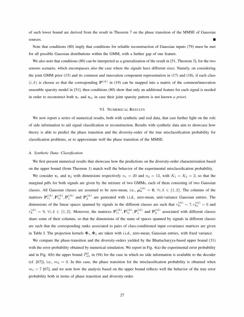
of such lower bound are derived from the result in Theorem 7 on the phase transition of the MMSE of Gaussian

sources.

Note that conditions (80) imply that conditions for reliable reconstruction of Gaussian inputs (79) must be met

for all possible Gaussian distributions within the GMM, with a further gap of one feature.

We also note that conditions (80) can be interpreted as a generalization of the result in [51, Theorem 3], for the two

sensors scenario, which encompasses also the case where the signals have different sizes. Namely, on considering

the joint GMM prior (15) and its common and innovation component representation in (17) and (18), if each class

(i, k) is chosen so that the corresponding P(ik) in (19) can be mapped into a matrix of the common/innovation

ensemble sparsity model in [51], then conditions (80) show that only an additional feature for each signal is needed

in order to reconstruct both x1 and x2, in case their joint sparsity pattern is not known a priori.

VI. NUMERICAL RESULTS

We now report a series of numerical results, both with synthetic and real data, that cast further light on the role

of side information to aid signal classification or reconstruction. Results with synthetic data aim to showcase how

theory is able to predict the phase transition and the diversity-order of the true misclassification probability for

classification problems, or to approximate well the phase transition of the MMSE.

A. Synthetic Data: Classification

We first present numerical results that showcase how the predictions on the diversity-order characterization based

on the upper bound (from Theorem 1) match well the behavior of the experimental misclassification probability.

We consider x1 and x2 with dimensions respectively n1 = 20 and n2 = 12, with K1 = K2 = 2, so that the

marginal pdfs for both signals are given by the mixture of two GMMs, each of them consisting of two Gaussian

classes. All Gaussian classes are assumed to be zero-mean, i.e., µ(ik)x = 0, ∀i, k ∈ {1, 2}. The columns of the

matrices P(ik)c1 ,P

(ik)c2 ,P

(ik)1 and P

(ik)2 are generated with i.i.d., zero-mean, unit-variance Gaussian entries. The

dimensions of the linear spaces spanned by signals in the different classes are such that r(ik)x1 = 7, r(ik)x2 = 6 and

r(ik)x = 9, ∀i, k ∈ {1, 2}. Moreover, the matrices P

(ik)c1 ,P

(ik)c2 ,P

(ik)1 and P

(ik)2 associated with different classes

share some of their columns, so that the dimensions of the sums of spaces spanned by signals in different classes

are such that the corresponding ranks associated to pairs of class-conditioned input covariance matrices are given

in Table I. The projection kernels Φ1,Φ2 are taken with i.i.d., zero-mean, Gaussian entries, with fixed variance.

We compare the phase-transition and the diversity-orders yielded by the Bhattacharyya-based upper bound (31)

with the error probability obtained by numerical simulation. We report in Fig. 4(a) the experimental error probability

and in Fig. 4(b) the upper bound PUerr in (94) for the case in which no side information is available to the decoder

(cf. [67]), i.e., m2 = 0. In this case, the phase transition for the misclassification probability is obtained when

m1 > 7 [67], and we note how the analysis based on the upper bound reflects well the behavior of the true error

probability both in terms of phase transition and diversity-order.

27

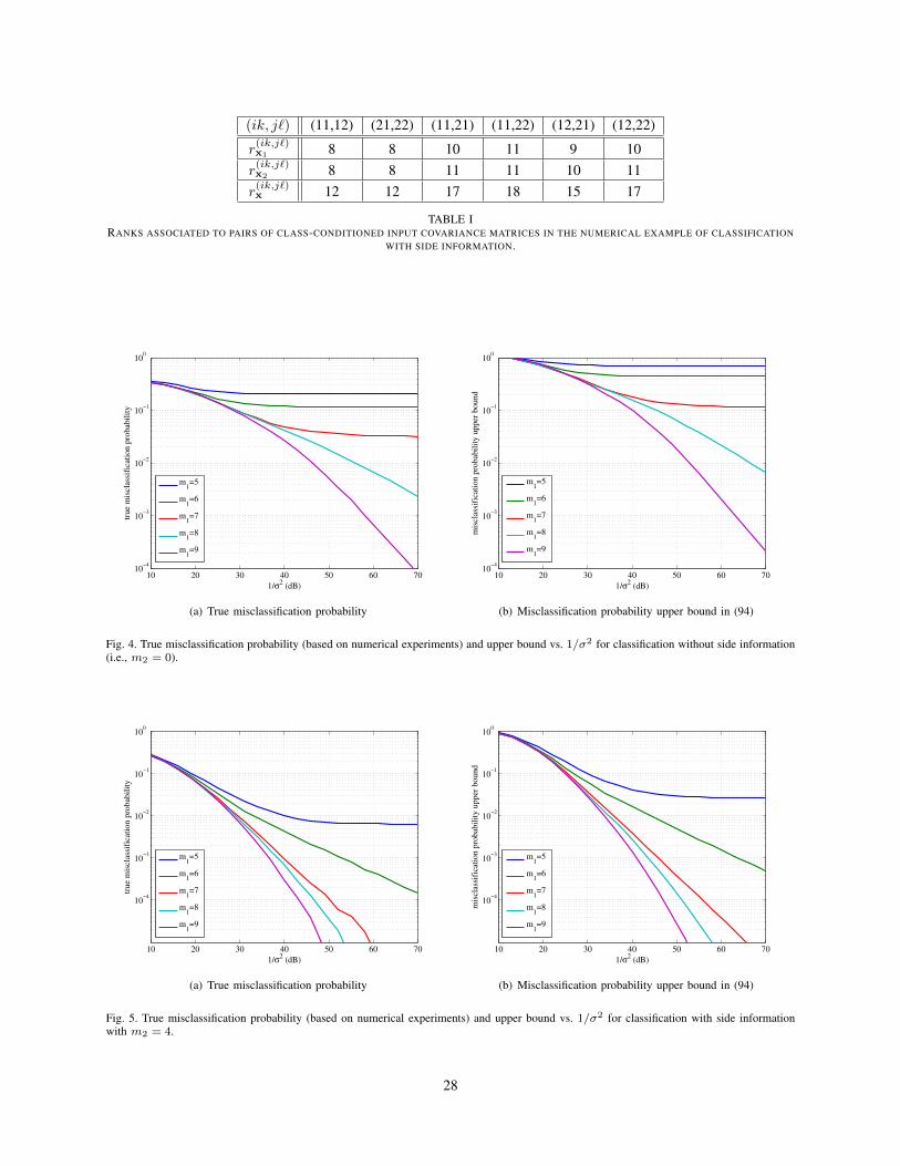
(ik, j`) (11,12) (21,22) (11,21) (11,22) (12,21) (12,22)

r(ik,j`)x1 8 8 10 11 9 10r(ik,j`)x2 8 8 11 11 10 11r(ik,j`)x 12 12 17 18 15 17

TABLE IRANKS ASSOCIATED TO PAIRS OF CLASS-CONDITIONED INPUT COVARIANCE MATRICES IN THE NUMERICAL EXAMPLE OF CLASSIFICATION

WITH SIDE INFORMATION.

10 20 30 40 50 60 7010

−4

10−3

10−2

10−1

100

1/σ2 (dB)

tru

e m

iscl

assi

fica

tio

n p

rob

abil

ity

m1=5

m1=6

m1=7

m1=8

m1=9

(a) True misclassification probability

10 20 30 40 50 60 7010

−4

10−3

10−2

10−1

100

1/σ2 (dB)

mis

clas

sifi

cati

on

pro

bab

ilit

y u

pp

er b

ou

nd

m1=5

m1=6

m1=7

m1=8

m1=9

(b) Misclassification probability upper bound in (94)

Fig. 4. True misclassification probability (based on numerical experiments) and upper bound vs. 1/σ2 for classification without side information(i.e., m2 = 0).

10 20 30 40 50 60 70

10−4

10−3

10−2

10−1

100

1/σ2 (dB)

tru

e m

iscl

assi

fica

tio

n p

rob

abil

ity

m1=5

m1=6

m1=7

m1=8

m1=9

(a) True misclassification probability

10 20 30 40 50 60 70

10−4

10−3

10−2

10−1

100

1/σ2 (dB)

mis

clas

sifi

cati

on

pro

bab

ilit

y u

pp

er b

ou

nd

m1=5

m1=6

m1=7

m1=8

m1=9

(b) Misclassification probability upper bound in (94)

Fig. 5. True misclassification probability (based on numerical experiments) and upper bound vs. 1/σ2 for classification with side informationwith m2 = 4.

28

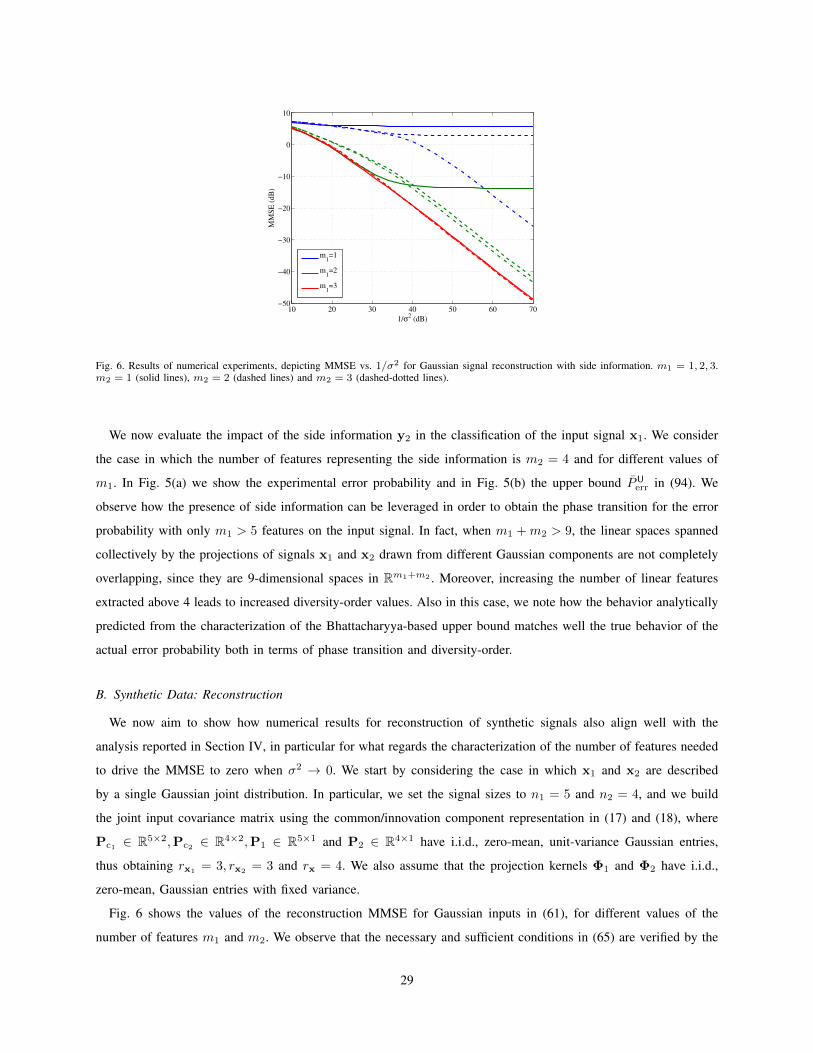
10 20 30 40 50 60 70−50

−40

−30

−20

−10

0

10

1/σ2 (dB)

MM

SE

(d

B)

m1=1

m1=2

m1=3

Fig. 6. Results of numerical experiments, depicting MMSE vs. 1/σ2 for Gaussian signal reconstruction with side information. m1 = 1, 2, 3.m2 = 1 (solid lines), m2 = 2 (dashed lines) and m2 = 3 (dashed-dotted lines).

We now evaluate the impact of the side information y2 in the classification of the input signal x1. We consider

the case in which the number of features representing the side information is m2 = 4 and for different values of

m1. In Fig. 5(a) we show the experimental error probability and in Fig. 5(b) the upper bound PUerr in (94). We

observe how the presence of side information can be leveraged in order to obtain the phase transition for the error

probability with only m1 > 5 features on the input signal. In fact, when m1 +m2 > 9, the linear spaces spanned

collectively by the projections of signals x1 and x2 drawn from different Gaussian components are not completely

overlapping, since they are 9-dimensional spaces in Rm1+m2 . Moreover, increasing the number of linear features

extracted above 4 leads to increased diversity-order values. Also in this case, we note how the behavior analytically

predicted from the characterization of the Bhattacharyya-based upper bound matches well the true behavior of the

actual error probability both in terms of phase transition and diversity-order.

B. Synthetic Data: Reconstruction

We now aim to show how numerical results for reconstruction of synthetic signals also align well with the

analysis reported in Section IV, in particular for what regards the characterization of the number of features needed

to drive the MMSE to zero when σ2 → 0. We start by considering the case in which x1 and x2 are described

by a single Gaussian joint distribution. In particular, we set the signal sizes to n1 = 5 and n2 = 4, and we build

the joint input covariance matrix using the common/innovation component representation in (17) and (18), where

Pc1 ∈ R5×2,Pc2 ∈ R4×2,P1 ∈ R5×1 and P2 ∈ R4×1 have i.i.d., zero-mean, unit-variance Gaussian entries,

thus obtaining rx1= 3, rx2

= 3 and rx = 4. We also assume that the projection kernels Φ1 and Φ2 have i.i.d.,

zero-mean, Gaussian entries with fixed variance.

Fig. 6 shows the values of the reconstruction MMSE for Gaussian inputs in (61), for different values of the

number of features m1 and m2. We observe that the necessary and sufficient conditions in (65) are verified by the

29

numerical results: in particular, when m2 = 1, the phase transition for the MMSE occurs only when m1 ≥ 3, when

m2 = 2, the phase transition is obtained with m1 ≥ 2 and, finally, when m2 = 3, a single feature extracted from

the input signal is sufficient to guarantee the phase transition.

We now consider signal reconstruction for GMM inputs. In particular, we assume that the vectors x1 and x2 are

drawn from the joint GMM prior described in Section VI-A for the case of signal classification, and we assume again

to use projection kernels with i.i.d., zero-mean, Gaussian entries. Reconstruction is performed via the conditional

mean estimator, that is now given by

x1(y) = E [x1|y] =

∫x1p(x1|y)dx1 (82)

=

∫x1

(∫p(x1,x2)p(y|x1,x1)∫

p(x)p(y|x)dxdx2

)dx1 (83)

=

∫x1

(∫ K1∑i=1

K2∑k=1

pC1,C2(i, k)N (x1,x2; µ(ik)

x , Σ(ik)x )dx2

)dx1 (84)

where [38]

pC1,C2(i, k) =

pC1,C2(i, k)N (y; Φµ(ik)x , σ2I + ΦΣ

(ik)x ΦT)∑K1

i=1

∑K2

k=1 pC1,C2(i, k)N (y; Φµ

(ik)x , σ2I + ΦΣ

(ik)x ΦT)

(85)

µ(ik)x = µ(ik)

x + Σ(ik)x ΦT(σ2I + ΦΣ(ik)

x ΦT)−1(y −Φµ(ik)x ) (86)

Σ(ik)x = Σ(ik)

x −Σ(ik)x ΦT(σ2I + ΦΣ(ik)

x ΦT)−1ΦΣ(ik)x , (87)

and we have used the notation N (x;µ,Σ) to express explicitly the argument of the Gaussian distribution. Then,

on marginalizing out x2, we obtain

x1(y) =

K1∑i=1

K2∑k=1

pC1,C2(i, k)(µ(ik)

x1+ [Σ(ik)

x1Σ(ik)

x12]ΦT(σ2I + ΦΣ(ik)

x ΦT)−1(y −Φµ(ik)x )

)(88)

and, as expected from the properties of the MMSE estimator [70], x1(y) can be also obtained by retaining the first

n1 entries of the joint conditional mean estimator x(y) = E [x|y] [38].

Fig. 7 shows the MMSE values for reconstruction both with side information (subfigure (a)), where we set m2 = 4,

and without side information (subfigure (b)), where we set m2 = 0. When side information is not available at the

decoder, the phase transition is obtained when m1 > max(i,k) r(ik)x1 = 7 [64]. On the other hand, as predicted by

the sufficient conditions in (69), the presence of side information allows to guarantee the phase transition with only

m1 > 5 features. Notice also in this case how the theoretical analysis matches well the behavior shown by the

numerical results.

C. Experimental Results: Natural Imaging

In this section, we consider a two-dimensional image compressive sensing example. The input signal is represented

in this case by the image “Lena” with resolution 512× 512 and the side information is given by a low-resolution

version of the same subject, which consists of 128 × 128 pixels (see Fig. 8). Note also that, as a low-resolution

30

10 20 30 40 50 60 70−25

−20

−15

−10

−5

0

5

10

15

20

25

1/σ2 (dB)

MM

SE

(d

B)

m1=5

m1=6

m1=7

m1=8

m1=9

(a) Without side information

10 20 30 40 50 60 70−40

−30

−20

−10

0

10

20

30

1/σ2 (dB)

MM

SE

(d

B)

m1=5

m1=6

m1=7

m1=8

m1=9

(b) With side information

Fig. 7. Results of numerical experiments, depicting MMSE vs. 1/σ2 for GMM signal reconstruction without and with side information, i.e.,m2 = 0 and m2 = 4, respectively.

Fig. 8. Left: input signal, high-resolution image (512×512). Right: side information, low-resolution image (128×128)

version of the signal of interest, side information in this case can be related to the scaling coefficients of the wavelet

transform of the input signal. Both images are then partitioned into non-overlapping patches, so that the input vector

x1 represents 8× 8 patches extracted from the 512× 512 picture and x2 represents 2× 2 patches extracted from

the low-resolution image. In this way, the input image and the side information are divided into the same number

of patches, which represent the same spatial portion of the subject (see [5], [64] for a detailed description of the

imaging setup) .

We assume that the signals x1 and x2 are described by a joint GMM as that in Section II-A, with K1 = K2 = 20.

The class variables C1 and C2 are assumed to be perfectly correlated, so that pC1,C2(i, k) = 0 if i 6= k. The

parameters of the joint GMM, i.e., the prior probabilities, the mean and the covariance matrices associated to each

31

0 10 20 30 40 50 60 7015

20

25

30

35

40

45

50

55

1/σ2 (dB)

PS

NR

(d

B)

m1=10

m1=11

m1=12

m1=13

m1=14

m1=15

m1=16

(a) Without side information

0 10 20 30 40 50 60 7015

20

25

30

35

40

45

50

55

60

65

1/σ2 (dB)

PS

NR

(d

B)

m1=10

m1=11

m1=12

m1=13

m1=14

m1=15

m1=16

(b) With side information

Fig. 9. Results of numerical experiments, depicting PSNR vs. 1/σ2 for reconstruction of the image “Lena” in Fig. 8 without and with sideinformation (Φ2 = I). Note that subfigures (a) and (b) have different scalings on the vertical axes.

Gaussian distribution within the GMM, are learned from the “Caltech 101” dataset [71], that does not include the test

image, via the expectation-maximization (EM) algorithm [72]. The covariance matrices Σ(ik)x ∈ R68×68 obtained

with the training algorithm have full rank. Therefore, in order to fit the trained model to an exactly low-rank GMM,

to showcase further how theory aligns with practice, we modify the covariance matrices by retaining only the first 15

principal components and setting to zero the remaining 53 eigenvalues. In this way, we obtain r(ik)x1 = 15, r(ik)x2 = 4

and r(ik)x = 15 for all (i, k) ∈ S . Moreover, patches extracted from the test image and the side information image

are also adapted to such low-dimensional model by projecting the vector x = [xT1 xT

2 ]T onto the 15-dimensional

subspace corresponding to the range of the matrix Σ(ik)x of the Gaussian distribution associated to each patch.

We notice that this procedure does not introduce substantial distortion, and the relative peak signal-to-noise ratio

(PSNR) values for the test image and the side information image are equal to 34 dB and 46 dB, respectively. This

is due to the fact that the eigenvalues of the trained covariance matrices decay exponentially fast, thus implying

that “almost low-rank” GMM priors model well patches extracted from natural images.

We consider the problem of reconstructing the test image “Lena” from noisy linear features, in the presence of

the side information represented by the low-resolution image. Linear features are extracted from the input signal via

the matrix Φ1 ∈ Rm1×n1 , which is generated with i.i.d., zero-mean, Gaussian entries with fixed variance. On the

other hand, we assume that the side information image is not compressed, i.e., we assume Φ2 = I. Reconstruction

is performed via the closed-form, conditional mean estimator (88).

Fig. 9 reports the PSNR vs. 1/σ2 curves obtained for different numbers of linear features extracted from the

test image patches. For comparison, we also show the corresponding curves for the case of reconstruction without

side information [64]. We clearly observe how the phase transition for reconstruction obtained with natural images

matches the predictions obtained with the mathematical analysis developed in Section IV. In particular, when side

32

information is not available at the decoder, the phase transition occurs when m1 > max(i,k) r(ik)x1 = 15 [64]. On

the other hand, the presence of side information allows for reliable reconstruction in the low-noise regime with a

reduced number of features extracted from each patch. Namely, in the case under consideration, the conditions (69)

are equivalent to m1 > 11, which is shown to match well the PSNR behavior in Fig. 9(b).

As already observed in [64], we underline the fact that the theory developed in Sections III and IV yields

significant results only for the case of low-rank GMMs rather than “approximately low-rank” models. On the other

hand, GMM priors obtained via learning algorithms applied to natural images are not exactly low-rank. In fact,

input covariance matrices obtained with such methods are typically described as

Σ(ik)x = Σ(ik)

x + εI, (89)

where Σ(ik)x is low-rank and the term εI accounts for the model mismatch between the real data and their projection

onto the principal components containing the majority of the information associated to the data. In this way, we can

observe that the feature extraction model in (3) with full-rank covariances Σ(ik)x is mathematically equivalent to a

feature extraction model akin to (3) with low-rank covariances Σ(ik)x and where the additive noise w is substituted

by additive noise with distribution N (0, εΦΦT + σ2I). Therefore, on noticing that the matrix ΦΦT approximate

well the identity matrices when Φ has non-zero entries that are i.i.d., zero-mean, Gaussian with unit variance, we

can conclude that performance associated to “approximately low-rank” models for a given noise variance σ2 is

comparable to the performance of the corresponding exactly low-rank models for noise variance equal to σ2 + ε.

D. Experimental Results: Compressive Hyperspectral Imaging

Finally, we present an example to showcase how the proposed framework also offers a principled approach to

design systems able to leverage effectively side information in reconstruction tasks. In this case, we do not reveal

the presence of phase transitions in the reconstruction error, due to the fact that the signal model describing the data

is a full-rank model. However, we can notice how side information can be used in order to improve reconstruction

performance.

We consider a compressive hyperspectral imaging example, in which hyperspectral images of a subject are recov-

ered from compressive measurements in the presence of side information. In particular, we consider measurements

collected by the coded aperture snapshot spectral imager (CASSI) apparatus described in [73]. Side information is

represented in this case by an RGB snapshot of the same scene, which can be easily obtained without requiring

expensive hyperspectral imaging devices. The information contained in the RGB image is expected to improve the

reconstruction quality of the input signal, also due to the fact that, in contrast to the measurements taken by the

CASSI camera, the RGB image is not affected by coded aperture modulation.

In this case the vector x1 represents patches extracted from the hyperspectral image, whereas x2 represents patches

extracted from the corresponding RGB image (see [73] for details on how data from this system are analyzed). The

vectors x1 and x2 are assumed to be modeled by the joint GMM described in Section II-A with K1 = K2 = 20.

33

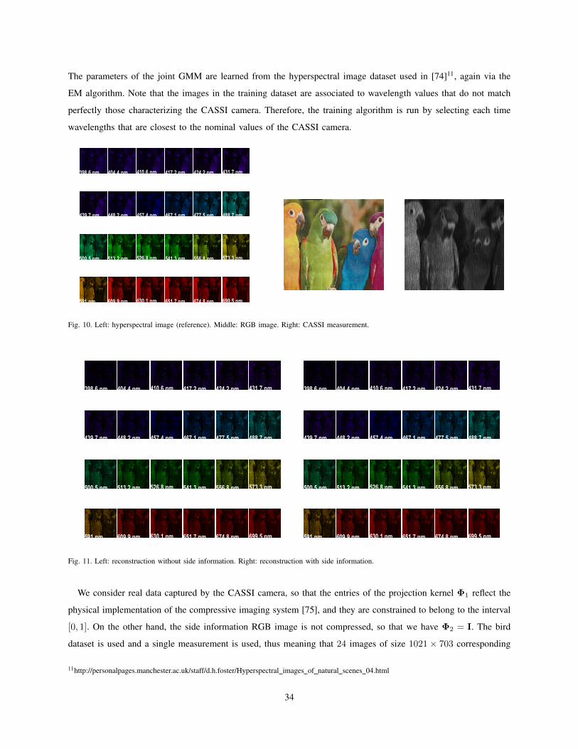
The parameters of the joint GMM are learned from the hyperspectral image dataset used in [74]11, again via the

EM algorithm. Note that the images in the training dataset are associated to wavelength values that do not match

perfectly those characterizing the CASSI camera. Therefore, the training algorithm is run by selecting each time

wavelengths that are closest to the nominal values of the CASSI camera.

398.6 nm 404.4 nm 410.6 nm 417.2 nm 424.2 nm 431.7 nm

439.7 nm 448.2 nm 457.4 nm 467.1 nm 477.5 nm 488.7 nm

500.5 nm 513.2 nm 526.8 nm 541.3 nm 556.8 nm 573.3 nm

591 nm 609.9 nm 630.1 nm 651.7 nm 674.8 nm 699.5 nm

Fig. 10. Left: hyperspectral image (reference). Middle: RGB image. Right: CASSI measurement.

398.6 nm 404.4 nm 410.6 nm 417.2 nm 424.2 nm 431.7 nm

439.7 nm 448.2 nm 457.4 nm 467.1 nm 477.5 nm 488.7 nm

500.5 nm 513.2 nm 526.8 nm 541.3 nm 556.8 nm 573.3 nm

591 nm 609.9 nm 630.1 nm 651.7 nm 674.8 nm 699.5 nm

398.6 nm 404.4 nm 410.6 nm 417.2 nm 424.2 nm 431.7 nm

439.7 nm 448.2 nm 457.4 nm 467.1 nm 477.5 nm 488.7 nm

500.5 nm 513.2 nm 526.8 nm 541.3 nm 556.8 nm 573.3 nm

591 nm 609.9 nm 630.1 nm 651.7 nm 674.8 nm 699.5 nm

Fig. 11. Left: reconstruction without side information. Right: reconstruction with side information.

We consider real data captured by the CASSI camera, so that the entries of the projection kernel Φ1 reflect the

physical implementation of the compressive imaging system [75], and they are constrained to belong to the interval

[0, 1]. On the other hand, the side information RGB image is not compressed, so that we have Φ2 = I. The bird

dataset is used and a single measurement is used, thus meaning that 24 images of size 1021× 703 corresponding

11http://personalpages.manchester.ac.uk/staff/d.h.foster/Hyperspectral images of natural scenes 04.html

34

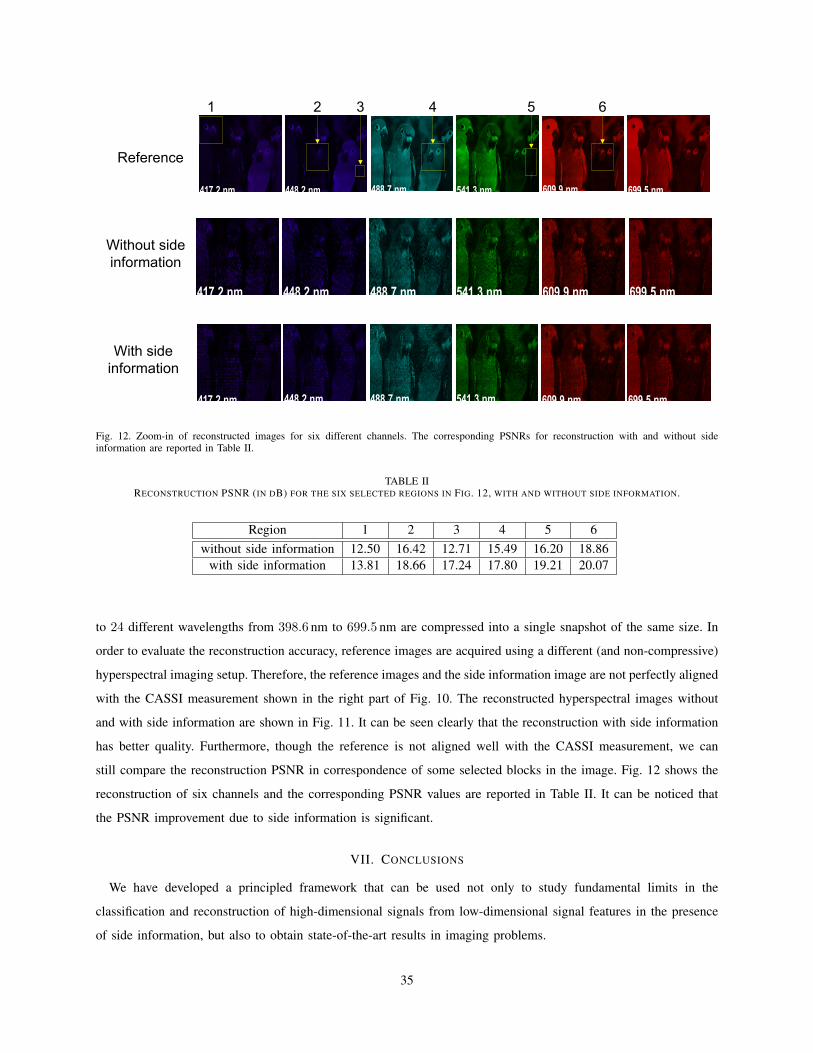
http://personalpages.manchester.ac.uk/staff/d.h.foster/Hyperspectral_images_of_natural_scenes_04.html

417.2 nm 448.2 nm 488.7 nm 541.3 nm 609.9 nm 699.5 nm

417.2 nm 448.2 nm 488.7 nm 541.3 nm 609.9 nm 699.5 nm

417.2 nm 448.2 nm 488.7 nm 541.3 nm 609.9 nm 699.5 nm

Reference

Without side information

With side information

1 2 3 4 5 6

Fig. 12. Zoom-in of reconstructed images for six different channels. The corresponding PSNRs for reconstruction with and without sideinformation are reported in Table II.

TABLE IIRECONSTRUCTION PSNR (IN DB) FOR THE SIX SELECTED REGIONS IN FIG. 12, WITH AND WITHOUT SIDE INFORMATION.

Region 1 2 3 4 5 6without side information 12.50 16.42 12.71 15.49 16.20 18.86

with side information 13.81 18.66 17.24 17.80 19.21 20.07

to 24 different wavelengths from 398.6 nm to 699.5 nm are compressed into a single snapshot of the same size. In

order to evaluate the reconstruction accuracy, reference images are acquired using a different (and non-compressive)

hyperspectral imaging setup. Therefore, the reference images and the side information image are not perfectly aligned

with the CASSI measurement shown in the right part of Fig. 10. The reconstructed hyperspectral images without

and with side information are shown in Fig. 11. It can be seen clearly that the reconstruction with side information

has better quality. Furthermore, though the reference is not aligned well with the CASSI measurement, we can

still compare the reconstruction PSNR in correspondence of some selected blocks in the image. Fig. 12 shows the

reconstruction of six channels and the corresponding PSNR values are reported in Table II. It can be noticed that

the PSNR improvement due to side information is significant.

VII. CONCLUSIONS

We have developed a principled framework that can be used not only to study fundamental limits in the

classification and reconstruction of high-dimensional signals from low-dimensional signal features in the presence

of side information, but also to obtain state-of-the-art results in imaging problems.

35

In particular, we have considered a linear feature-extraction model, where a decoder has access to noisy linear

features of both the signal of interest and the side information signal, in order to carry out either classification or

reconstruction. We have also considered a model where the joint distribution of the signal of interest and the side

information, conditioned on some underlying class labels is a multivariate Gaussian, which embodies the correlation

between these signals. The marginal distribution of the signal conditioned on a class label is a Gaussian mixture,

and likewise the marginal distribution of the side information conditioned on the class label is also a Gaussian

mixture.

This modeling approach, which can be used to encapsulate a wide range of distributions, has then offered the

opportunity to capitalize on tractable bounds to the misclassification probability and the reconstruction error, to

construct an asymptotic characterization of the behavior of these quantities in the low-noise regime. In addition,

this modeling approach has also led to a characterization of sharp sufficient conditions for a phase transition in the

misclassification probability and necessary and sufficient conditions for the phase transition of the reconstruction

error (the performance quantities under consideration), as a function of the geometry of the sources, the geometry

of the linear feature extraction process and their interplay, reminiscent of the Slepian-Wolf and the Wyner-Ziv

conditions.

It has been shown that our theory is well aligned with practice via a range of numerical results associated with low-

rank data models. Of particular relevance, it has also been shown that our framework offers a principled mechanism

to integrate side information in data classification and reconstruction problems in the context of compressive

hyperspectral imaging in the presence of side information.

This work also points to various possible future directions:

• It is of interest to extend the results from consideration of only one side information source to settings where

there are multiple sources of side information. It is possible to generalize the models immediately, but the

analysis is considerably more complex (as pointed out in Appendix A).

• There is interest in generalization of the results from the scenario where the linear features are extracted

randomly to scenarios where the linear features are designed [5], [6], [64] (or indeed nonlinear features are

designed [21]) is relevant. This could lead to additional gains in the phase transition.

• The generalization of the results from scenarios where only the decoder has access to the side information to

scenarios where both the encoder and the decoder have access to the side information is also relevant. This

may also lead to additional gains both in the presence of random linear features or designed ones.

• Finally, it is believed that the framework, which applies to settings where both the signal of interest and the side

information signal follow correlated Gaussian mixture models, can also be generalized to other data models

– this can then translate into applications of the framework to scenarios where signals conform to different

modalities.

36

APPENDIX A

PROOF OF THEOREM 1

We start by considering the case, K1 = 2. We recall that the Batthacharyya upper bound for the misclassification

probability of C1 is given by

Perr =√pC1(1)pC1(2)

∫ √p(y|C1 = 1)p(y|C1 = 2)dy (90)

=√pC1

(1)pC1(2)

∫ √√√√ K2∑k.`=1

pC2|C1(k|1)pC2|C1

(`|2)p(y|C1 = 1, C2 = k)p(y|C1 = 2, C2 = `)dy. (91)

An upper and a lower bound to the expression in (91) are simply obtained by considering the following fact.

Given n non-negative numbers a1, . . . , an ≥ 0, it holds

1√n

n∑i=1

√ai ≤

√√√√ n∑i=1

ai ≤n∑i=1

√ai, (92)

where the first inequality derives from the concavity of the function f(x) =√x and the second inequality can be

simply proved by induction starting from n = 2.

Then, an upper bound to Perr is obtained as

PUerr =

√pC1

(1)pC1(2)

K2∑k.`=1

√pC2|C1

(k|1)pC2|C1(`|2)

∫ √p(y|C1 = 1, C2 = k)p(y|C1 = 2, C2 = `)dy, (93)

and, similarly, a lower bound is given by P Lerr = PU

err/K2. The generalization of this result to the case K1 > 2, is

based on the evaluation of the union bound (31), which, together with (92), yields the upper bound

PUerr =

K1∑i=1

K1∑j=1j 6=i

pC1(i)

K2∑k.`=1

√pC2|C1

(k|i)pC2|C1(`|j)

∫ √p(y|C1 = i, C2 = k)p(y|C1 = j, C2 = `)dy, (94)

and the corresponding lower bound P Lerr = PU

err/K2.

Note that the lower and the upper bounds differ only by the multiplicative constant K2. Therefore, they are tight

bounds in terms of the diversity-order, and it is possible to derive the diversity-order associated to Perr from the

analysis of such bounds.

We now observe that the integral in (94) also appears in the analysis of the upper bound to the misclassification

probability associated to the classification between two Gaussian distributions without side information as described

in [67]. In particular, such integral can be expressed as∫ √p(y|C1 = i, C2 = k)p(y|C1 = j, C2 = `)dy = e−K(ik,j`), (95)

37

where

K(ik, j`) =1

8(µ(ik)

x − µ(j`)x )TΦT

[Φ(Σ

(ik)x + Σ

(j`)x )ΦT + 2σ2I

2

]−1Φ(µ(ik)

x − µ(j`)x )

+1

2log

det(

Φ(Σ(ik)x +Σ(j`)

x )ΦT+2σ2I2

)√

det(ΦΣ(ik)x ΦT + σ2I)

√det(ΦΣ

(j`)x ΦT + σ2I)

. (96)

For the case of zero-mean classes, i.e., assuming µ(ik)x = µ

(j`)x = 0, a low-noise expansion for the integral in (94)

is given by [67, Theorem 1]

e−K(ik,j`) = A(ik,j`) · (σ2)d(ik,j`) + o(

(σ2)d(ik,j`)), (97)

for a fixed constant A(ik,j`) > 0, and with d(ik, j`) given by

d(ik, j`) =1

2

(r(ik,j`) − r(ik) + r(j`)

2

), (98)

where


x ΦT)

, r(j`) = rank(ΦΣ(j`)

x ΦT)

, r(ik,j`) = rank(Φ(Σ(ik)

x + Σ(j`)x )ΦT

). (99)

Therefore, we can conclude that a low-noise expansion for the upper bound of the misclassification probability (31)

is given by

Perr(σ2) = A · (σ2)d + o

((σ2)d

), (100)

where A > 0 is a fixed constant and

d = mini 6=j∈{1,...,K1}

mink,`∈{1,...,K2}

d(ik, j`) = mini,k,j,`,i 6=j

d(ik, j`). (101)

is the worst-case diversity-order associated to the misclassification of pairs of Gaussian distributions identified by

the index pairs (i, k) and (j, `), such that i 6= j.

It is then clear that the computation of the expansion of Perr for classification with side information requires the

computation of the diversity-order terms (98), and, therefore, the computation of the ranks r(ik) = rank(Γ(ik)) and

r(ik,j`) = rank(Γ(ik,j`)), with Γ(ik) = ΦP(ik) and Γ(ik,j`) = ΦP(ik,j`), where

P(ik) =

P(ik)c1 P

(ik)1 0

P(ik)c2 0 P

(ik)2

(102)

P(ik,j`) =

P(ik,j`)c1 P

(ik,j`)1 0

P(ik,j`)c2 0 P

(ik,j`)2

(103)

and

Φ =

Φ1 0

0 Φ2

. (104)

38

Therefore, in the following we will provide a characterization of such ranks as a function of the numbers of

features m1 and m2. For ease of a compact notation, we drop superscripts when results hold for all possible choices

of index pairs (i, k) or quadruples (i, k, j, `). For the ease of notation, we will assume in the following n1 ≥ m1

and n2 ≥ m2. However, the extension to the case where n1 < m1 or n2 < m2 is straightforward.

Lemma 1: Let Pc1 ∈ Rn1×sc ,Pc2 ∈ Rn2×sc ,P1 ∈ Rn1×s1 ,P2 ∈ Rn2×s2 . Let Φ ∈ R(m1+m2)×(n1+n2) as

in (104), such that the row spaces associated to Φ1 and Φ2 are m1− and m2−dimensional spaces, isotropically

distributed at random in Rn1 and Rn2 , respectively, and let P as

P =

Pc1 P1 0

Pc2 0 P2

. (105)

Then, with probability 1, the rank of the matrix Γ = ΦP is given by

r = rank(Γ) = min {rx,min{m1, rx1}+ min{m2, rx2

}} , (106)

where rx1= rank[Pc1 P1], rx2

= rank[Pc2 P2] and rx = rank(P).

Proof: It is easy to observe that the expression in (106) represents an upper bound to the rank r = rank(ΦP) as

rank(ΦP) ≤ rank(P) and rank(Γ) is always less than or equal to the sum of the ranks of the matrices obtained by

considering separately its first m1 and the remaining m2 rows, i.e., rank(Φ1[Pc1 P1 0]) and rank(Φ2[Pc2 0 P2]).

Therefore, in the rest of the proof, we will aim at showing that such upper bound is actually tight, by proving that

we can find at least r linear independent columns in Γ.

We start by considering the special case in which we impose Φ2 = In2, and we show that in this case it holds

rI2 = rank

Φ1 0

0 I

Pc1 P1 0

Pc2 0 P2

= min{rx,min{m1, rx1}+ rx2

}. (107)

On recalling Sylvester’s rank theorem [76], which states

rank(AB) = rank(B)− dim(Im(B) ∩Null(A)), (108)

we can write

rI2 = rank(P)− dim

Im(P) ∩Null

Φ1 0

0 I

. (109)

Then, we consider the matrix Ψ1 ∈ Rn1×(n1−m1), whose columns form a basis for the null space Null(Φ1), which

is isotropically distributed among the (n1−m1)-dimensional spaces in Rn1 . It is then straightforward to show that

the columns of the matrix [ΨT1 0T

n2×(n1−m1)]T span the null space

Null

Φ1 0

0 I

(110)

39

and we can write

rI2 = rx − dim

Im(P) ∩ Im

Ψ1

0

(111)

= rank

Pc1 P1 0 Ψ1

Pc2 0 P2 0

− (n1 −m1), (112)

in which we have leveraged the rank equality for block matrices [77],

rank [A B] = rank(A) + rank(B)− dim(Im(A) ∩ Im(B)), (113)

and the fact that rank(Ψ1) = n1 −m1 and rank(P) = rx. Consider now the computation of the rank

rΨ1= rank

Pc1 P1 0 Ψ1

Pc2 0 P2 0

. (114)

In order to compute such rank, we will leverage the generalized singular value decomposition (GSVD) as described

in [78]. In particular, consider two matrices A ∈ Rn×p and B ∈ Rm×p, with the same number of columns, and

with rA = rank(A), rB = rank(B), rAB = rank[ATBT]T and sAB = rA + rB − rAB. Then, there exist two

orthogonal matrices U ∈ Rn×n,V ∈ Rm×m and a non-singular matrix X ∈ Rp×p such that

UTAX = [ΛA 0n×(p−rAB)] , UTBX = [ΛB 0m×(p−rAB)], (115)

where

ΛA =

rAB−rB sAB rAB−rA

rAB−rB I

sAB DA

n−rA 0

, ΛB =

rAB−rB sAB rAB−rA

m−rB 0

sAB DB

rAB−rA I

. (116)

and DA = diag(α1, . . . , αsAB), DB = diag(β1, . . . , βsAB

), such that 1 < α1 ≤ · · · ≤ αsAB< 0 and 0 < β1 ≤

· · · ≤ βsAB< 1, and α2

i + β2i = 1, for i = 1, . . . , sAB.

Therefore, on applying the GSVD to the two matrices [Pc1 P1 0] and [Pc2 0 P2], we can write

rΨ1 = rank

UT 0

0 VT

Pc1 P1 0 Ψ1

Pc2 0 P2 0

X 0

0 In1−m1

(117)

= rank

Λ1 0 Ψ′1

Λ2 0 0

(118)

40

where

Λ1 =

rx−rx2 rx1+rx2−rx rx−rx1

rx−rx2I

rx1+rx2

−rx D1

n1−rx1 0

, Λ2 =

rx−rx2 rx1+rx2−rx rx−rx1

n2−rx20

rx1+rx2

−rx D2

rx−rx1 I

(119)

and where Ψ′1 = UTΨ1 is a matrix whose column space is still isotropically distributed at random among the

(n1 −m1)−dimensional subspaces of Rn1 . Now, by considering the first rx − rx2 columns of the matrix in (118)

together with its last n1 −m1 columns, given the fact the columns in Ψ′1 form a random space in Rn1 , we can

conclude that, with probability 1, we can pick from such columns min{rx − rx2+ n1 − m1, n1} independent

columns, which are also independent from the remaining (rx1+ rx2

− rx) + (rx − rx1) = rx2

non-zero columns

of the same matrix. Therefore, we have

rΨ1 = min{rx − rx2 + n1 −m1, n1}+ rx2 (120)

and then

rI2 = min{rx − rx2+ n1 −m1, n1}+ rx2

− (n1 −m1) (121)

= min{rx,m1 + rx2} (122)

= min{rx,min{m1, rx1}+ rx2

}, (123)

where the last equality is obtained by observing that rx ≤ rx1+ rx2

.

Consider now the general case, in which Φ2 is not forced to be equal to the identity matrix. In this case, by

leveraging (123), we can write

r = rank

Φ1 0

0 Φ2

Pc1 P1 0

Pc2 0 P2

(124)

= rank

Φ1 0

0 I

Pc1 P1 0

Φ2Pc2 0 Φ2P2

(125)

= min{rI1 ,min{m1, rx1}+ min{m2, rx2}}, (126)

in which we have introduced the symbol

rI1 = rank

Pc1 P1 0

Φ2Pc2 0 Φ2P2

(127)

= rank

I 0

0 Φ2

Pc1 P1 0

Pc2 0 P2

, (128)

and where we have used the fact that rank[Φ2Pc2 0 Φ2P2] = min{m2, rx2}. Then, with a procedure similar to

41

that used to compute rI2 , it is possible to show that rI1 = min{rx, rx1+ min{m2, rx2

}}, thus leading to

r = min {min{rx, rx1+ min{m2, rx2

}},min{m1, rx1}+ min{m2, rx2

}} (129)

= min{rx,min{m1, rx1}+ min{m2, rx2

}}. (130)

Finally, note that Lemma 1 can be immediately applied to compute r(ik), r(j`) and r(ik,j`), thus concluding the

proof of Theorem 1.

We also note in passing that the generalization of Lemma 1 to the case of multiple side information sources,

x2,x3, . . . ,xL, seems to be considerably more complex, due to the absence of a transform akin to the GSVD in

(115) and (116) that jointly diagonalizes more than two matrices.

APPENDIX B

PROOF OF COROLLARY 1

On the basis of the low-noise regime expansion for the upper bound to the misclassification probability (31)

contained in Theorem 1, we can state that the phase transition (32) occurs if and only if d > 0, which is equivalent

to d(ik, j`) > 0, ∀(i, k, j, `) ∈ SSIC. Moreover, on observing that the matrices ΦΣ(ik)x ΦT and ΦΣ

(j`)x ΦT are

positive semidefinite, we can immediately state that d(ik, j`) = 0 if and only if r(ik,j`) = r(ik) = r(j`), which is

verified if only if [64, Lemma 2]

ImΦΣ(ik)x ΦT = ImΦΣ(j`)

x ΦT. (131)

Then, r(ik,j`)x = r(ik)x = r

j`)x implies that ImΣ

(ik)x = ImΣ

(j`)x and, therefore, (131) holds regardless of the expression

of the projection kernel Φ, thus leading to d(ik, j`) = 0.

Assume now r(ik,j`)x > r

(ik)x , r

j`)x . We can then use the rank expression (106) and consider separately the following

cases:

1) r(ik,j`)x1 > r

(ik)x1 , r


(ik)x2 , r

(j`)x2 : in this case, if m1 > min{r(ik)x1 , r

(j`)x1 } or m2 > min{r(ik)x2 , r

(j`)x2 },

we can immediately conclude that d(ik, j`) > 0, by simply considering the classification from the observation

of y1 or y2 alone, respectively, and by leveraging the results in [67, Theorem 2]. On the other hand, if

we assume m1 ≤ min{r(ik)x1 , r(j`)x1 },m2 ≤ min{r(ik)x2 , r

(j`)x2 } and m1 + m2 > min{r(ik)x , r

(j`)x }, then we

have r(ik) = min{r(ik)x ,m1 + m2}, r(j`) = min{r(j`)x ,m1 + m2} and r(ik,j`) = min{r(ik,j`)x ,m1 + m2}.

Then, since m1 + m2 > min{r(ik)x , r(j`)x }, we have immediately that r(ik,j`) > min{r(ik), r(j`)}, and

thus d(ik, j`) > 0. Such sufficient conditions on the minimum number of measurements m1,m2 needed

to guarantee d(ik, j`) > 0 are also necessary. In fact, if m1 ≤ min{r(ik)x1 , r(j`)x1 },m2 ≤ min{r(ik)x2 , r

(j`)x2 } and

m1 +m2 ≤ min{r(ik)x , r(j`)x }, then r(ik,j`) = r(ik) = r(j`) = m1 +m2.

2) r(ik,j`)x1 = r

(ik)x1 = r


(ik)x2 = r

(j`)x2 : in this case, we note that min{m1, r

(ik)x1 }+min{m2, r

(ik)x2 } =

min{m1, r(j`)x1 } + min{m2, r

(j`)x2 } = min{m1, r

(ik,j`)x1 } + min{m2, r

(ik,j`)x2 } = D, and then d(ik, j`) > 0 if

and only if D > min{r(ik)x , r(j`)x }. Then, we can split the analysis in further subcases as follows:

42

• if m1 ≤ r(ik)x1 and m2 ≤ r(ik)x2 , then d(ik, j`) > 0 if and only if m1 +m2 > min{r(ik)x , r(j`)x };

• if m1 > r(ik)x1 and m2 ≤ r(ik)x2 , then d(ik, j`) > 0 if and only if m2 > min{r(ik)x − r(ik)x1 , r

(j`)x − r(j`)x1 };

• if m1 ≤ r(ik)x1 and m2 > r(ik)x2 , then d(ik, j`) > 0 if and only if m1 > min{r(ik)x − r(ik)x2 , r

(j`)x − r(j`)x2 };

• if m1 > r(ik)x1 and m2 > r

(ik)x2 , then r

(ik)x1 + r

(ik)x2 = r

(j`)x1 + r

(j`)x2 > min{r(ik)x , r

(j`)x } and therefore

d(ik, j`) > 0.

Finally, we can combine the previous expressions to obtain necessary and sufficient conditions to guarantee

d(ik, j`) > 0 as m1 > min{r(ik)x − r(ik)x2 , r

(j`)x − r(j`)x2 }



. (132)

3) r(ik,j`)x1 > r

(ik)x1 , r

(j`)x1 and r

(ik,j`)x2 = r

(ik)x2 = r

(j`)x2 : we can prove immediately that, in this case, if m1 >

min{r(ik)x1 , r(j`)x1 }, then d(ik, j`) > 0, simply by considering classification based on the observation of only

y1. Assume now m1 ≤ min{r(ik)x1 , r(j`)x1 }. Then, it holds r(ik) = min{r(ik)x ,m1 + min{m2, r

(ik)x2 }}, r(j`) =

min{r(j`)x ,m1 + min{m2, r(j`)x2 }} and r(ik,j`) = min{r(ikj`)x ,m1 + min{m2, r

(ik,j`)x2 }}, and, on observing

that min{m2, r(ik)x2 } = min{m2, r

(j`)x2 } = min{m2, r

(ik,j`)x2 }, we have immediately that d(ik, j`) > 0 if

and only if min{r(ik)x , r(j`)x } < m1 + min{m2, r

(ik)x2 }. In particular, if m2 ≤ r

(ik)x2 , then, d(ik, j`) > 0

if and only if m1 + m2 > min{r(ik)x , r(j`)x }, whereas if m2 > r

(ik)x2 , then d(ik, j`) > 0 if and only if

m1 > min{r(ik)x − r(ik)x2 , r(j`)x − r(j`)x2 }. Finally, on combining these expressions, we can write necessary and

sufficient conditions for d(ik, j`) > 0 as


} or



. (133)

4) r(ik,j`)x1 = r

(ik)x1 = r

(j`)x1 and r

(ik,j`)x2 > r

(ik)x2 , r

(j`)x2 : the proof for this case follows steps similar to the case

r(ik,j`)x1 > r

(ik)x1 , r


(ik)x2 = r

(j`)x2 .

APPENDIX C

PROOF OF THEOREM 2

The characterization of the low-noise expansion of the upper bound to the misclassification probability in (31) for

the case of nonzero-mean classes starts from the analysis of its lower and upper bounds presented in Appendix A.

We focus on the expressions in (94), (95) and (96), and we leverage the low-noise expansion of the integral in (95)

presented in [67, Theorem 3] for the case of two nonzero-mean Gaussian classes. Namely, we recall that

e−K(ik,j`) = B(ik,j`) · e−C(ik,j`)/σ2

+ o(e−C

(ik,j`)/σ2), (134)

for fixed constants B(ik,j`), C(ik,j`) > 0 if and only if

Φ(µ(ik)x − µ(j`)

x ) /∈ Im(Φ(Σ(ik)

x + Σ(j`)x )ΦT

). (135)

43

Otherwise, the integral in (95) can be expanded as in (97). Therefore, if condition (135) is verified for all the index

quadruples (i, k, j, `) ∈ SSIC, then we can expand the upper bound to the misclassification probability in (31) as

Perr(σ2) = B · e−C/σ

2

+ o(e−C

/σ2), (136)

for fixed constants B,C > 0. Otherwise, the upper bound of the misclassification probability is expanded as

Perr(σ2) = A · (σ2)d + o

((σ2)d

), (137)

for a fixed A > 0 and where

d = min(i,k,j,`)∈S′

d(ik, j`), (138)

where S ′ is the set of the index quadruples (i, k, j, `) ∈ SSIC for which (135) is not verified and d(ik, j`) is as

in (98).

We can now provide necessary and sufficient conditions on m1 and m2 such that (135) is verified. We observe

that (135) holds if and only if r(ik,j`)µ > r(ik,j`), where we have defined

r(ik,j`)µ = rank

Φ1 0

0 Φ2

µ(ik)x1 − µ

(j`)x1 P

(ik,j`)c1 P

(ik,j`)1 0

µ(ik)x2 − µ

(j`)x2 P

(ik,j`)c2 0 P

(ik,j`)2

. (139)

Assume first that µ(ik)x −µ

(j`)x ∈ Im

(Σ

(ik)x + Σ

(j`)x

). Then r(ik,j`)µ = r(ik,j`), and, therefore (135) does not hold,

irrespectively of the exact matrix Φ.

Assume now µ(ik)x − µ

(j`)x /∈ Im

(Σ

(ik)x + Σ

(j`)x

). We can use the rank expression (106) and similar steps to

those in the proof of Corollary 1 in order to consider separately the following cases:

1) µ(ik)x1 − µ

(j`)x1 /∈ Im(Σ

(ik)x1 + Σ

(j`)x1 ) and µ

(ik)x2 − µ

(j`)x2 /∈ Im(Σ

(ik)x2 + Σ

(j`)x2 ): on leveraging [64, Lemma 3],

we can observe that if m1 > r(ik,j`)x1 or m2 > r

(ik,j`)x2 , then (135) holds, as the upper bound to the error

probability obtained by classification based on the observation of y1 or y2 alone, respectively, decreases

exponentially with 1/σ2. On the other hand, if m1 ≤ r(ik,j`)x1 ,m2 ≤ r

(ik,j`)x2 and m1 + m2 > r

(ik,j`)x , then

it holds r(ik,j`)µ = min{r(ik,j`)x + 1,m1 +m2} > r(ik,j`) and thus (135) is verified. The previous conditions

are also shown to be necessary by noting that, if m1 ≤ r(ik,j`)x1 ,m2 ≤ r

(ik,j`)x2 and m1 +m2 ≤ r

(ik,j`)x , then

r(ik,j`)µ = r(ik,j`) = m1 +m2.

2) µ(ik)x1 −µ

(j`)x1 ∈ Im(Σ

(ik)x1 +Σ

(j`)x1 ) and µ

(ik)x2 −µ

(j`)x2 ∈ Im(Σ

(ik)x2 +Σ

(j`)x2 ): in this case, r(ik,j`)µ = min{r(ik,j`)x1,x2 +

1,min{m1, r(ik,j`)x1 }+min{m2, r

(ik,j`)x2 }}, so that (135) holds if and only if min{m1, r

(ik,j`)x1 }+min{m2, r

(ik,j`)x2 } >

r(ik,j`)x . Then, we can split the analysis in the following subcases:

• if m1 ≤ r(ik,j`)x1 and m2 ≤ r(ik,j`)x , then (135) is verified if and only if m1 +m2 > r(ik,j`)x ;

• if m1 > r(ik,j`)x1 and m2 ≤ r(ik,j`)x , then (135) is verified if and only if m2 > r

(ik,j`)x − r(ik,j`)x1 ;

• if m1 ≤ r(ik,j`)x1 and m2 > r(ik,j`)x , then (135) is verified if and only if m1 > r

(ik,j`)x − r(ik,j`)x2 ;

44

• if m1 > r(ik,j`)x1 and m2 > r

(ik,j`)x then (135) is verified, since

r(ik,j`)x1+r(ik,j`)x2

= rank[µ(ik)x1−µ(j`)

x1P(ik,j`)

c1 P(ik,j`)1 ]+rank[µ(ik)

x2−µ(j`)

x2P(ik,j`)

c2 P(ik,j`)2 ] ≥ r(ik,j`)x +1.

(140)

Finally, we can combine the previous expressions and write necessary and sufficient conditions to guarantee

(135) as m1 > r

(ik,j`)x − r(ik,j`)x2


m1 +m2 > r(ik,j`)x

. (141)

3) µ(ik)x1 −µ

(j`)x1 /∈ Im(Σ

(ik)x1 + Σ

(j`)x1 ) and µ

(ik)x2 −µ

(j`)x2 ∈ Im(Σ

(ik)x2 + Σ

(j`)x2 ): in this case, if m1 > r

(ik,j`)x , then

we can state that (135) is true by considering simply classification on the basis of the observation of y1 alone.

Therefore, assume now that m1 ≤ r(ik,j`)x . In this case r(ik,j`)µ = min{r(ik,j`)x + 1,m1 + min{m2, r(ik,j`)x2 }}.

Therefore, if m2 ≤ r(ik,j`)x2 , then (135) holds if and only if m1 + m2 > r

(ik,j`)x . On the other hand, if

m2 > r(ik,j`)x2 , then (135) holds if and only if m1 > r

(ik,j`)x − r

(ik,j`)x2 . We can combine the previous

expressions and write necessary and sufficient conditions to guarantee (135) in this case as

m1 > r(ik,j`)x1or


m1 +m2 > r(ik,j`)x

. (142)

4) µ(ik)x1 − µ

(j`)x1 ∈ Im(Σ

(ik)x1 + Σ

(j`)x1 ) and µ

(ik)x2 − µ

(j`)x2 /∈ Im(Σ

(ik)x2 + Σ

(j`)x2 ): the proof for this case follows

steps similar to the case µ(ik)x1 − µ

(j`)x1 /∈ Im(Σ

(ik)x1 + Σ

(j`)x1 ) and µ

(ik)x2 − µ

(j`)x2 ∈ Im(Σ

(ik)x2 + Σ

(j`)x2 ).

APPENDIX D

PROOF OF THEOREM 3

We start by proving that conditions (65) are sufficient in order to drive the MMSE to zero in the low-noise

regime. The first condition in (65) is trivial, as it reflects the fact that it is possible to drive the reconstruction

MMSE to zero in the low-noise regime from the observation of y1 alone, provided that m1 ≥ rx1[64].

Consider now the upper bound associated to the distributed classification problem, i.e., the MMSE incurred in

recovering both x1 and x2 from y1 and y2 (or, equivalently, x from y). Then, we can write

MMSEG1|1,2(σ2) ≤ MMSEG

1,2|1,2(σ2) (143)

= tr(Σx −ΣxΦT

(σ2I + ΦΣxΦT

)−1ΦΣx

)(144)

and we can follow steps similar to those in [64, Appendix B] to show that, in the low-noise regime, MMSEG1,2|1,2(σ2)

approaches zero if and only if

rank(ΦΣxΦT

)= rank (Σx) . (145)

45

In fact, we can introduce the eigenvalue decomposition

Σ12x ΦTΦΣ

12x = UΣΛUT

Σ, (146)

where Λ = diag(λ1, . . . , λrΣ , 0, . . . , 0), with rΣ = rank(Σ

12x ΦTΦΣ

12x

), and by using the inversion Lemma [79,

§0.7.4] we can write

MMSEG1,2|1,2(σ2) = tr

(Σx

(I + 1/σ2Σ

12x ΦTΦΣ

12x

)−1)(147)

= tr(ΣxUΣ

(I + 1/σ2Λ

)−1UT

Σ

)(148)

= tr(ΣxUΣΛUT

Σ

), (149)

where Λ = diag(

11+λ1/σ2 , . . . ,

11+λrΣ

/σ2 , 1, . . . , 1)

. It is then clear that MMSEG1,2|1,2(σ2) approaches zero, when

σ2 → 0, if and only if

Null(Σ

12x ΦTΦΣ

12x

)⊆ Null (Σx) . (150)

Moreover, on noting that Null (Σx) ⊆ Null(Σ

12x ΦTΦΣ

12x

), we immediately conclude that (150) is equivalent to

(145).

We can now determine conditions on the number of features m1 and m2 needed in order to verify (145) by

leveraging the rank expression (106). In particular, note that (145) holds if and only if

min{m1, rx1}+ min{m2, rx2} ≥ rx. (151)

We can consider separately four different cases, and observe that, if m1 ≤ rx1 and m2 ≤ rx2 , then (145) is verified

if and only if m1 + m2 ≥ rx. If m1 ≤ rx1and m2 > rx2

, then (145) holds if and only if m1 ≥ rx − rx2and

symmetrically, m1 > rx1and m2 ≤ rx2

, then (145) holds if and only if m2 ≥ rx − rx1. Finally, m1 > rx1

and

m2 > rx2 , then (145) always holds since rx1 + rx2 ≥ rx. Then, the four previous cases can be summarized by

stating that (145) is true if and only if m1 and m2 verify the conditionsm1 ≥ rx − rx2

m2 ≥ rx − rx1

m1 +m2 ≥ rx

. (152)

Then, the proof of sufficiency is concluded by simply considering the union of the set of values (m1,m2) which

verify (152) with the set m1 ≥ rx1.

We now prove that conditions (65) are also necessary to guarantee that the MMSE approaches zero when σ2 → 0.

In the remainder of this proof, we denote the MMSE associated to the estimation of the random vector u from the

observation vector v by

MMSE(u|v) = E[‖u− E [u|v] ‖2

], (153)

where the expectation is taken with respect to the joint distribution of (u,v). Then, we obtain a lower bound to

46

MMSEG1|1,2(σ2) by observing that, for all σ2 > 0, we have

MMSEG1|1,2(σ2) = MMSE(x1|y1,y2) ≥ MMSE(x1|y1,y2,w1,w2) = MMSE(x1|Φ1x1,Φ2x2). (154)

On the other hand, by observing that the MMSE does not depend on the value of the mean of the input signal

to estimate, and by taking the expectation in the right hand side of (154) with respect to the random variables

x1|Φ2x2 and Φ2x2, separately, it is possible to show that

MMSE(x1|Φ1x1,Φ2x2) = MMSE(z|Φ1z), (155)

where z ∈ Rn1 is a Gaussian vector with covariance matrix equal to the conditional covariance of x1 given Φ2x2,

i.e., z ∼ N (0,Σz), where

Σz = Cov(x1|Φ2x2) = Σx1 −Σx12ΦT2 (Φ2Σx2Φ

T2 )†Φ2Σx21 . (156)

Then, by leveraging the result in [64, Theorem 1], or by simply considering the set of linear equations corresponding

to the rows of the matrix Φ1Σ1/2z , a necessary condition for MMSE(z|Φ1z) = 0, and therefore, a necessary condition

for limσ2→0 MMSEG1|1,2(σ2) = 0, is given by

m1 ≥ rz = rank(Σz). (157)

We complete the proof by computing the rank rz using a result on the generalized Schur complement of a positive

semidefinite matrix [80]. Namely, Σz can be viewed as the generalized Schur complement of the block Φ2Σx2ΦT2

of the positive semidefinite matrix

Σx1Φ2x2= E

x1

Φ2x2

[xT1 (Φ2x2)T]

=

Σx1Σx12

ΦT2

Φ2Σx21Φ2Σx2

ΦT2

, (158)

and, with probability 1, we have [80]

rank(Σx1Φ2x2) = rz + rank(Φ2Σx2ΦT2 ) = rz + min{m2, rx2}. (159)

In addition, on considering the matrix

ΣΦ2x2x1= E

Φ2x2

x1

[(Φ2x2)T xT1 ]

=

Φ2Σx2ΦT2 Φ2Σx21

Σx12ΦT

2 Σx1

, (160)

and on applying the same rank computation, we also have

rank(ΣΦ2x2x1) = rank(Σx1Φ2x2) = rx1 + rank(Cov(Φ2x2|x1)) = rx1 + rank(Φ2(Σx2 −Σx21Σ

†x1

Σx12)ΦT2

).

(161)

Then, on recalling that the projection kernel Φ2 is rotation-invariant, and by using again the generalized Schur

47

complement rank computation, with probability 1, we have

rank(Cov(Φ2x2|x1)) = min{m2, rx − rx1}. (162)

Finally, by substituting (161) and (162) in (159), we can rewrite (157) as

m1 ≥ rx1 −min{m2, rx2}+ min{m2, rx − rx1}, (163)

which can be immediately shown to be equivalent to conditions (65), thus concluding the necessity part of the

proof.

APPENDIX E

PROOF OF THEOREM 4

This proof in based on steps similar to those in [64, Appendix C]. Nevertheless, we report here the key ideas

used in the proof for completeness. On defining

W(ik)x1

= µ(ik)x1

+ W(ik)x1

(y −Φµ(ik)

x

), (164)

where W(ik)x1 is as in (68), and by using the law of total probability, we can write

MSECR(σ2) ≤∑i,k

pC1,C2(i, k) E[‖x1 −W(ik)

x1(y)‖2|C1 = i, C2 = k

]+∑i,k

pC1,C2(i, k)

∑(j,`) 6=(i,k)

p(C1 = j, C2 = `|C1 = i, C2 = k)

·E[‖x1 −W(j`)

x1(y)‖2|C1 = j, C2 = `, C1 = i, C2 = k

]. (165)

We can observe immediately that, assuming the conditions in (69) are verified, Theorem 3 guarantees that the terms

E[‖x1 −W(ik)

x1 (y)‖2|C1 = i, C2 = k]

approach zero when σ2 → 0. Then, we are left with proving

limσ2→0

p(C1 = j, C2 = `|C1 = i, C2 = k) E[‖x1 −W(j`)

x1(y)‖2|C1 = j, C2 = `, C1 = i, C2 = k

]= 0 (166)

whenever (j, `) 6= (i, k). Given the conditions (69) hold, if m1 > r(ik)x1 and m1 > r

(j`)x1 , then we can leverage

the result in [64, Appendix C] on the reconstruction of x1 from y1 alone to show that (166) holds. Otherwise, if

m1 ≤ r(ik)x1 or m1 ≤ r(j`)x1 , then (69) implies that m2 > r(ik)x −r(ik)x1 or m2 > r

(j`)x −r(j`)x1 respectively. At this point,

we can consider separately two cases: i) r(ik,j`)x > r(ik)x , r

(j`)x and ii) r(ik,j`)x = r

(ik)x = r

(j`)x . In the first case, the

range spaces Im(Σ(ik)x ) and Im(Σ

(j`)x ) are distinct, and we can leverage the characterization of the misclassification

probability of the distributed classification problem in order to prove (166). In particular, by following steps similar

to those in the proof of Corollary 1, we can show that

limσ2→0

p(C1 = j, C2 = `|C1 = i, C2 = k) = 0. (167)

48

Therefore, observe that the misclassification probability p(C1 = j, C2 = `|C1 = i, C2 = k) is the measure of the

set representing the decision region of the MAP classifier for the distributed classification problem associated to

the classes (j, `) with respect to the Gaussian measure induced by the Gaussian distribution of classes (i, k). Then,

it is also possible to show that, in the limit σ2 → 0, the product in (166) is upper bounded by the integral of a

measurable function over a set with measure zero, and then it converges to zero.

In the second case, instead, we have Im(Σ(ik)x ) = Im(Σ

(j`)x ), and we can consider separately further two cases.

If

µ(ik)x − µ(ik)

x /∈ Im(Σ(ik)x + Σ(j`)

x ) = Im(Σ(ik)x ), (168)

then Theorem 2 states that p(C1 = j, C2 = `|C1 = i, C2 = k) approaches zero in the low-noise regime, and we

can prove that (166) holds by following a similar procedure to that used for case i). On the other hand, if

µ(ik)x − µ(ik)

x ∈ Im(Σ(ik)x + Σ(j`)

x ) = Im(Σ(ik)x ), (169)

then the misclassification probability is not guaranteed to approach zero in the low-noise regime. However, on using

the law of total probability and the definition of MSE, we can notice that the argument of the limit in (166) is

upper bounded by E[‖x1 −W(j`)

x1 (y)‖2|C1 = i, C2 = k]

and that

E[‖x1 −W(j`)

x1(y)‖2|C1 = i, C2 = k

]≤ E

[‖x−W(j`)

x (y)‖2|C1 = i, C2 = k], (170)

where

W(j`)x (y) = µ(j`)

x + W(j`)x

(y −Φµ(j`)

x

)(171)

and

W(j`)x = Σ(j`)

x ΦT(σ2I + ΦΣ(j`)

x ΦT)−1

. (172)

Then, we can show that the right hand side of (170) approaches zero when σ2 → 0 by using steps similar to

those in [64, Appendix C-B]. This reflects the fact that the mismatched MSE for Gaussian sources reaches zero in

the low-noise regime, provided that the estimated input covariance has the same range space than the true input

covariance. In particular, on denoting by Σ(ik)y = σ2I + ΦΣ

(ik)x ΦT the covariance matrix of y conditioned on

(C1, C2) = (i, k), and on introducing the symbol M(ik,j`) = (µ(ik)x − µ

(j`)x )(µ

(ik)x − µ

(j`)x )T, we can write

MSE(ik,j`)(σ2) = E[‖x−W(j`)

x (y)‖2|C1 = i, C2 = k]

(173)

= E

[tr

((x−W(j`)

x (y))(

x−W(j`)x (y)

)T)|C1 = i, C2 = k

](174)

= tr(Σ(ik)

x

)− 2tr

(W(ik)

x Σ(ik)y (W(j`)

x )T)

+ tr(W(j`)

x Σ(ik)y (W(j`)

x )T)

+ tr(M(ik,j`)

)−2tr

(M(ik,j`)ΦT(Wj`

x )T)

+ tr(ΦW(j`)

x M(ik,j`)(W(j`)x )T

), (175)

49

and we can prove that

limσ2→0

tr(W(ik)

x Σ(ik)y (W(j`)

x )T)

= tr(Σ(ik)x ); (176)

limσ2→0

tr(W(j`)

x Σ(ik)y (W(j`)

x )T)

= tr(Σ(ik)x ); (177)

limσ2→0

tr(M(ik,j`)(W(j`)

x )T)

= tr(M(ik,j`)

); (178)

limσ2→0

tr(W(j`)

x ΦM(ik,j`)ΦT(W(j`)x )T

)= tr

(M(ik,j`)

). (179)

The proof is based on the use of the inversion Lemma [79]

A(Ic−1 + BA)−1B = I− (I + cAB)−1, (180)

in which we choose A = ΦT and B = ΦΣ(j`)x and we write

tr(W(ik)

x Σ(ik)y (W(j`)

x )T)

= tr(Σ(ik)

x ΦT(Iσ2 + ΦΣ(j`)x ΦT)−1ΦΣ(j`)

x

)(181)

= tr(Σ(ik)

x

)− tr

(Σ(ik)

x (I +1

σ2ΦTΦΣ(j`)

x )−1). (182)

Then, on noting that the matrix ΦTΦΣ(j`)x is diagonalizable with probability 1, and by following steps similar

to those adopted in the proof of Theorem 3, we are able to prove (176). Finally, also (177), (178) and (179) are

proved by following a completely similar approach.

REFERENCES

[1] R. O. Duda, P. E. Hart, and D. G. Stork, Pattern Classification (2nd Edition). New York, NY: Wiley-Interscience, 2000.

[2] A. K. Jain, R. P. W. Duin, and J. Mao, “Statistical pattern recognition: A review,” IEEE Trans. Pattern Anal. Mach. Intell., vol. 22, no. 1,

pp. 4–37, 2000.

[3] J. Han and M. Kamber, Data Mining: Concepts and Techniques. Morgan Kaufmann Publishers, 2001.

[4] I. Guyon and A. Elisseeff, “An introduction to variable and feature selection,” J. Mach. Lear. Res., vol. 3, pp. 1157–1182, 2003.

[5] W. R. Carson, M. Chen, M. R. D. Rodrigues, R. Calderbank, and L. Carin, “Communications-inspired projection design with applications

to compressive sensing,” SIAM J. Imag. Sciences, vol. 5, no. 4, pp. 1185–1212, 2012.

[6] M. Chen, W. Carson, M. R. D. Rodrigues, R. Calderbank, and L. Carin, “Communications inspired linear discriminant analysis,” in Int.

Conf. Machine Learn. (ICML), Jun.-Jul. 2012.

[7] D. Erdogmus and J. C. Principe, “Lower and upper bounds for misclassification probability based on Renyi’s information,” J. VLSI Signal

Process. Syst. Signal Image Video Technol., vol. 37, no. 2 -3, pp. 305–317, 2004.

[8] K. Hild, D. Erdogmus, K. Torkkola, and J. Principe, “Feature extraction using information-theoretic learning,” IEEE Trans. Pattern Anal.

Mach. Intell., vol. 28, no. 9, pp. 1385–1392, 2006.

[9] S. Kaski and J. Peltonen, “Informative discriminant analysis,” in Int. Conf. Machine Learn. (ICML), 2003, pp. 329–336.

[10] L. Liu and P. Fieguth, “Texture classification from random features,” IEEE Trans. Pattern Anal. Mach. Intell., vol. 34, no. 3, pp. 574–586,

Mar. 2012.

[11] Z. Nenadic, “Information discriminant analysis: Feature extraction with an information-theoretic objective,” IEEE Trans. Pattern Anal.

Mach. Intell., vol. 29, no. 8, pp. 1394–1407, Aug. 2007.

[12] D. Tao, X. Li, X. Wu, and S. Maybank, “Geometric mean for subspace selection,” IEEE Trans. Pattern Anal. Mach. Intell., vol. 31, no. 2,

pp. 260–274, 2009.

50

[13] K. Torkkola, “Learning discriminative feature transforms to low dimensions in low dimensions,” in Advances in neural information

processing systems, 2001, pp. 969–976.

[14] ——, “Feature extraction by non-parametric mutual information maximization,” J. Mach. Learn. Res., vol. 3, pp. 1415–1438, Mar. 2003.

[15] J. Wright, A. Y. Yang, A. Ganesh, S. Sankar Sastry, and Y. Ma, “Robust face recognition via sparse representation,” IEEE Trans. Pattern

Anal. Mach. Intell., vol. 31, no. 2, pp. 210–227, Feb. 2009.

[16] B. Adcock, A. C. Hansen, C. Poon, and B. Roman, “Breaking the coherence barrier: A new theory for compressed sensing,” arXiv preprint

arXiv:1302.0561, 2013.

[17] B. Roman, A. Hansen, and B. Adcock, “On asymptotic structure in compressed sensing,” arXiv preprint arXiv:1406.4178, 2014.

[18] L. Wang, D. Carlson, M. Rodrigues, D. Wilcox, R. Calderbank, and L. Carin, “Designed measurements for vector count data,” in Advances

in neural information processing systems, 2013, pp. 1142–1150.

[19] L. Wang, D. Carlson, M. Rodrigues, R. Calderbank, and L. Carin, “A bregman matrix and the gradient of mutual information for vector

poisson and gaussian channels,” IEEE Trans. Inf. Theory, vol. 60, no. 5, pp. 2611–2629, May 2014.

[20] J. Tenenbaum, V. de Silva, and J. Langford, “A global geometric framework for nonlinear dimensionality reduction,” Science, vol. 290,

no. 5500, pp. 2319–2323, Dec. 2000.

[21] L. Wang, A. Razi, M. R. D. Rodrigues, R. Calderbank, and L. Carin, “Nonlinear information-theoretic compressive measurement design,”

in Int. Conf. Machine Learn. (ICML), Jun. 2014.

[22] E. Candes, J. K. Romberg, and T. Tao, “Stable signal recovery for incomplete and inaccurate measurements,” Comm. Pure Appl. Math.,

vol. 59, no. 8, pp. 1207–1223, 2006.

[23] E. Candes and T. Tao, “Near-optimal signal recovery from random projections: Universal encoding strategies?” IEEE Trans. Inf. Theory,

vol. 52, no. 12, pp. 5406–5425, 2006.

[24] D. Donoho, “Compressed sensing,” IEEE Trans. Inf. Theory, vol. 52, no. 4, pp. 1289–1306, 2006.

[25] E. Candes and T. Tao, “Decoding by linear programming,” IEEE Trans. Inf. Theory, vol. 51, no. 12, pp. 4203–4215, 2005.

[26] E. Candes, J. Romberg, and T. Tao, “Robust uncertainty principles: exact signal reconstruction from highly incomplete frequency

information,” IEEE Trans. Inf. Theory, vol. 52, no. 2, pp. 489–509, 2006.

[27] R. G. Baraniuk, M. Davenport, R. DeVore, and M. Wakin, “A simple proof of the restricted isometry property for random matrices,”

Constr. Approx., vol. 28, pp. 253–263, Dec. 2008.

[28] S. Mallat and Z. Zhang, “Matching pursuits with time-frequency dictionaries,” IEEE Trans. Signal Process., vol. 41, no. 12, pp. 3397–3415,

1993.

[29] S. S. Chen, D. L. Donoho, and M. A. Saunders, “Atomic decomposition by basis pursuit,” SIAM J. Sci. Comput., vol. 20, no. 1, pp. 33–61,

1998.

[30] J. A. Tropp and S. J. Wright, “Computational methods for sparse solution of linear inverse problems,” Proc. IEEE, vol. 98, no. 6, pp.

948–958, 2010.

[31] M. Davenport, P. Boufounos, M. Wakin, and R. Baraniuk, “Signal processing with compressive measurements,” IEEE J. Sel. Topics Signal

Process., vol. 4, no. 2, pp. 445–460, 2010.

[32] T. Blumensath and M. Davies, “Sampling theorems for signals from the union of finite-dimensional linear subspaces,” IEEE Trans. Inf.

Theory, vol. 55, no. 4, pp. 1872–1882, 2009.

[33] M. Stojnic, F. Parvaresh, and B. Hassibi, “On the reconstruction of block-sparse signals with an optimal number of measurements,” IEEE

Trans. Signal Process., vol. 57, no. 8, pp. 3075–3085, 2009.

[34] Y. C. Eldar and M. Mishali, “Robust recovery of signals from a structured union of subspaces,” IEEE Trans. Inf. Theory, vol. 55, no. 11,

pp. 5302–5316, 2009.

[35] Y. Eldar, P. Kuppinger, and H. Bolcskei, “Block-sparse signals: Uncertainty relations and efficient recovery,” IEEE Trans. Signal Process.,

vol. 58, no. 6, pp. 3042–3054, 2010.

[36] R. G. Baraniuk, V. Cevher, M. F. Duarte, and C. Hedge, “Model-based compressive sensing,” IEEE Trans. Inf. Theory, vol. 56, no. 4, pp.

1982–2001, 2010.

[37] R. G. Baraniuk and M. B. Wakin, “Random projections of smooth manifolds,” Found. of Comput. Math., vol. 9, no. 1, pp. 51–77, 2009.

[38] M. Chen, J. Silva, J. Paisley, D. Dunson, and L. Carin, “Compressive sensing on manifolds using a nonparametric mixture of factor

analyzers: Algorithm and performance bounds,” IEEE Trans. Signal Process., vol. 58, no. 12, pp. 6140–6155, 2010.

51

[39] M. Crouse, R. Nowak, and R. Baraniuk, “Wavelet-based statistical signal processing using hidden markov models,” IEEE Trans. Signal

Process., vol. 46, no. 4, pp. 886–902, 1998.

[40] D. Slepian and J. Wolf, “Noiseless coding of correlated information sources,” IEEE Trans. Inf. Theory, vol. 19, no. 4, pp. 471–480, 1973.

[41] R. Ahlswede and J. Korner, “Source coding with side information and a converse for degraded broadcast channels,” IEEE Trans. Inf.

Theory, vol. 21, no. 6, pp. 629–637, 1975.

[42] A. Wyner and J. Ziv, “The rate-distortion function for source coding with side information at the decoder,” IEEE Trans. Inf. Theory,

vol. 22, no. 1, pp. 1–10, 1976.

[43] T. M. Cover and J. A. Thomas, Elements of Information Theory. New York, NY: Wiley, 1991.

[44] N. Vaswani and W. Lu, “Modified-cs: Modifying compressive sensing for problems with partially known support,” IEEE Trans. Signal

Process., vol. 58, no. 9, pp. 4595–4607, 2010.

[45] C. Herzet, C. Soussen, J. Idier, and R. Gribonval, “Exact recovery conditions for sparse representations with partial support information,”

IEEE Trans. Inf. Theory, vol. 59, no. 11, pp. 7509–7524, 2013.

[46] X. Wang and J. Liang, “Side information-aided compressed sensing reconstruction via approximate message passing,” arXiv preprint

arXiv:1311.0576, 2013.

[47] G.-H. Chen, J. Tang, and S. Leng, “Prior image constrained compressed sensing (PICCS): a method to accurately reconstruct dynamic CT

images from highly undersampled projection data sets,” Med.l Phys., vol. 35, no. 2, pp. 660–663, 2008.

[48] L. Weizman, Y. C. Eldar, and D. B. Bashat, “The application of compressed sensing for longitudinal mri,” arXiv preprint arXiv:1407.2602,

2014.

[49] J. F. Mota, N. Deligiannis, and M. R. Rodrigues, “Compressed sensing with prior information: Optimal strategies, geometry, and bounds,”

arXiv preprint arXiv:1408.5250, 2014.

[50] D. Baron, M. B. Wakin, M. F. Duarte, S. Sarvotham, and R. G. Baraniuk, “Distributed compressed sensing,” arXiv preprint arXiv:0901.3403,

2009.

[51] M. Duarte, M. Wakin, D. Baron, S. Sarvotham, and R. Baraniuk, “Measurement bounds for sparse signal ensembles via graphical models,”

IEEE Trans. Inf. Theory, vol. 59, no. 7, pp. 4280–4289, 2013.

[52] A. Yang, M. Gastpar, R. Bajcsy, and S. Sastry, “Distributed sensor perception via sparse representation,” Proceedings of the IEEE, vol. 98,

no. 6, pp. 1077–1088, 2010.

[53] S. Haghighatshoar, “Multi terminal probabilistic compressed sensing,” arXiv preprint arXiv:1401.2569, 2014.

[54] D. Donoho, A. Javanmard, and A. Montanari, “Information-theoretically optimal compressed sensing via spatial coupling and approximate

message passing,” IEEE Trans. Inf. Theory, vol. 59, no. 11, pp. 7434–7464, 2013.

[55] A. Eftekhari, H. L. Yap, C. J. Rozell, and M. B. Wakin, “The restricted isometry property for random block diagonal matrices,” Appl.

Comput. Harmon. Anal., 2014.

[56] A. Hormati, O. Roy, Y. Lu, and M. Vetterli, “Distributed sampling of signals linked by sparse filtering: Theory and applications,” IEEE

Trans. Signal Process., vol. 58, no. 3, pp. 1095–1109, 2010.

[57] S. Ji, D. Dunson, and L. Carin, “Multitask compressive sensing,” IEEE Trans. Signal Process., vol. 57, no. 1, pp. 92–106, 2009.

[58] S. Ji, Y. Xue, and L. Carin, “Bayesian compressive sensing,” IEEE Trans. Signal Process., vol. 56, no. 6, pp. 2346–2356, 2008.

[59] H. W. Sorenson and D. L. Alspach, “Recursive Bayesian estimation using Gaussian sums,” Automatica, vol. 7, no. 4, pp. 465–479, 1971.

[60] G. Yu and G. Sapiro, “Statistical compressed sensing of Gaussian mixture models,” IEEE Trans. Signal Process., vol. 59, no. 12, pp.

5842–5858, 2011.

[61] G. Yu, G. Sapiro, and S. Mallat, “Solving inverse problems with piecewise linear estimators: From Gaussian mixture models to structured

sparsity,” IEEE Trans. Image Process., vol. 21, no. 5, pp. 2481–2499, 2012.

[62] J. Duarte-Carvajalino, G. Yu, L. Carin, and G. Sapiro, “Task-driven adaptive statistical compressive sensing of Gaussian mixture models,”

IEEE Trans. Signal Process., vol. 61, no. 3, pp. 585–600, 2013.

[63] J. Yang, X. Yuan, X. Liao, P. Llull, D. Brady, G. Sapiro, and L. Carin, “Video compressive sensing using Gaussian mixture models,” IEEE

Trans. Image Process., vol. 23, no. 11, pp. 4863–4878, 2014.

[64] F. Renna, R. Calderbank, L. Carin, and M. R. D. Rodrigues, “Reconstruction of signals drawn from a gaussian mixture via noisy compressive

measurements,” IEEE Trans. Signal Process., vol. 62, no. 9, pp. 2265–2277, 2014.

52

[65] H. Reboredo, F. Renna, R. Calderbank, and M. R. D. Rodrigues, “Compressive classification,” in IEEE Int. Symp. Information Theory

(ISIT), Jul. 2013.

[66] H. Reboredo, F. Renna, R. Calderbank, and M. Rodrigues, “Projections designs for compressive classification,” in IEEE Global Conf. Sig.

Inf. Process. (GlobalSIP), Dec. 2013, pp. 1029–1032.

[67] H. Reboredo, F. Renna, R. Calderbank, and M. R. D. Rodrigues, “Compressive classification of a mixture of Gaussians: Analysis, designs

and geometrical interpretation,” arXiv preprint arXiv:1401.6962v1, 2014.

[68] V. Tarokh, N. Seshadri, and A. R. Calderbank, “Space-time codes for high data rate wireless communication: Performance criterion and

code construction,” IEEE Trans. Inf. Theory, vol. 44, no. 2, pp. 744–765, 1998.

[69] V. Tarokh, H. Jafarkhani, and R. Calderbank, “Space-time block codes from orthogonal designs,” IEEE Trans. Inf. Theory, vol. 45, no. 5,

pp. 1456–1467, 1999.

[70] T. Kailath, A. H. Sayed, and B. Hassibi, Linear Estimation. Upper Saddle River, NJ: Prentice Hall, 2000.

[71] L. Fei-Fei, R. Fergus, and P. Perona, “One-shot learning of object categories,” IEEE Trans. Pattern Anal. Mach. Intell., vol. 28, pp.

594–611, 2006.

[72] C. M. Bishop, Pattern Recognition and Machine Learning (Information Science and Statistics). Secaucus, NJ, USA: Springer-Verlag

New York, Inc., 2006.

[73] A. Rajwade, D. Kittle, T.-H. Tsai, and L. Carin, “Coded hyperspectral imaging and blind compressive sensing,” SIAM Journal on Imaging

Sciences, vol. 6, no. 2, pp. 782–812, 2013.

[74] D. Foster, K. Amano, S. Nascimento, and M. Foster, “Frequency of metamerism in natural scenes,” Journal of the Optical Society of

America A, vol. 23, no. 12, pp. 2359–2372, 2006.

[75] D. Kittle, K. Choi, A. Wagadarikar, and D. J. Brady, “Multiframe image estimation for coded aperture snapshot spectral imagers,” Applied

Optics, vol. 49, no. 36, pp. 6824–6833, 2010.

[76] C. D. Meyer, Matrix analysis and applied linear algebra. Siam, 2000, vol. 2.

[77] Y. Tian and G. P. Styan, “Rank equalities for idempotent matrices with applications,” J. Com. Appl. Math., vol. 191, no. 1, pp. 77–97,

2006.

[78] C. C. Paige and M. A. Saunders, “Towards a generalized singular value decomposition,” SIAM J. Numer. Anal., vol. 18, no. 3, pp. 398–405,

1981.

[79] R. Horn and C. Johnson, Matrix Analysis. Cambridge, UK: Cambridge University Press, 1985.

[80] B.-Y. Wang, X. Zhang, and F. Zhang, “Some inequalities on generalized Schur complements,” Linear Algebra Appl., vol. 302, pp. 163–172,

1999.

53

1 classiﬁcation and reconstruction of high-dimensional

Documents