UNIT 12 TABULATION AND GRAPHICAL REPRESENTATION OF DATA

Structure

12.1 Introduction

12.2 Objectives

12.3 Meaning of Data

12.4 Nature of Data

12.4.1 Qualitative and Quantitative Data 12.4.2 Continuous and Discrete Data 12.4.3 Primary and Secondary Data

1 2.5 Measurement Scales

12.6 Meaning of Statistics

12.7 Need and Importance of Statistics

12.8 Importance of the Organisation of Data

12.9 Presentation of Data in a Sequence

12.10 Grouping and Tabulation of Data

12.1 1 Graphical Representation of Data

12.12 Types of Graphical Representation of Data

12.12.1 Histogram 12.12.2 Bar Diagram or Bar Graph 12.12.3 Frequency Polygon 12.12.4 Cumulative Frequency Curve or Ogive

12.13 Let Us Sum Up

12.14 Unit-end Exercises

! 12.15 Points for Discussion

12.16 Answers to Check Your Progress

1 12.17 Suggested Readings I

12.1 INTRODUCTION

In Block 11, you have studied about the learner's evaluation. For learner's evaluation, we usually administer a number of tests on all students of the class and scores are given in their answer-scripts. Often these are used as such, without interpreting them. If you have to interpret the scores, you must learn to tabulate them in a meaningful way and calculate various statistics from the same. In this Unit, you will study about the meaning and nature of data; the need and importance of statistics; the tabulation of data in a meaningful way and various types of graphical representation to make the data easily comprehendible.

Various types of statistics and the methods of their computation are being discussed in the subsequent units of this block itself.

'12.2 OBJECTIVES

After going through this unit, you will be able to:

understand the meaning and nature of data;

distinguish between the four measurement scales; 5

Techniques of understand the need, importance and meaning of statistics;

appreciate the importance of the organisation of data;

tabulate the data obtained by you in the classroom in a meaningful way;

app~teciate the advantages of graphical representation of data;

use appropriate graphic representation, for the data obtained by you in the classroom; and

interpret the data given in the form of graphical representation.

12.3 MEANING OF DATA

You might be reading a newspaper regularly. Almost every newspaper gives the minimum and the maximum temperatures recorded in the city on the previous day. It also indicates the rainfall recorded, and the time of sunrise and sunset. In your school, you regularly take attendance of children and record it in a register. For a patient, the doctor advises recording of the body temperature of the patient at regular intervals.

If you record the minimum and maximum temperature, or rainfall, or the time of sunrise and sunset, or attendance of children, or the body temperature of the patient, over a period of time, what you are recording is known as data. Here, you are recording the data of minimum and maximu& temperature of the city, data of rainfall, data for the time of sunrise and sunset, and the data pertaining to the attendance of children.

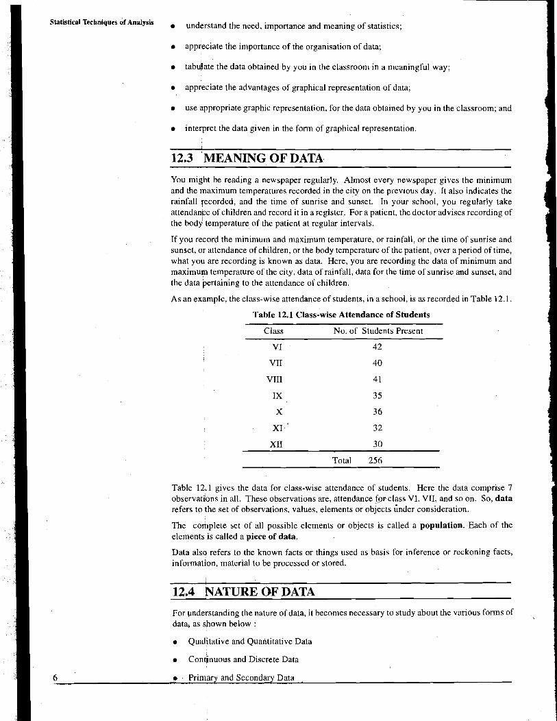
As an example, the class-wise attendance of students, in a school, is as recorded in Table 12.1.

Table 12.1 Class-wise Attendance of Students

Class No. of Students Present

VI 42

VII 40

VIII

XI .

XI1 30

Total 256

Table 12.1 gives the data for class-wise attendance of students. Here the data comprise 7 observations in all. These observations are, attendance fgr class VI, VII, and so on. So, data refers to the set of observations, values, elements or objects h d e r consideration.

The complete set of all possible elements or objects is called a population. Each of the elements is called a piece of data.

Data alsd refers to the known facts or things used as basis for inference or reckoning facts, information, material to be processed or stored.

12.4 NATURE OF DATA

For understanding the nature of data, it becomes necessary to study about the various forms of ,$

data, as shown below :

Qualitative and Quantitative Data

Continuous and Discrete Data

I L Primpry and Secondary Data

12.4.1 Qualitative and Quantitative Data Tabulation and Graphical Representation of Data

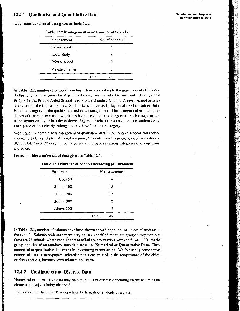
Let us consider a set of data given in Table 12.2.

Table 12.2 Management-wise Number of Schools

Management No. of Schools

Government 4

Local Body

Private Aided

Private Unaided - - - - -

Total 24

1 In Table 12.2, number of schools have been shown according to the management of schools. So the schools have been classified into 4 categories, namely, Government Schools, Local Body Schools, Private Aided Schools and Private Unaided Schools. A given school belongs to any one of the four categories. Such data is shown as Categorical or Qualitative Data. Here the category or the quality referred to is management. Thus categorical or qualitative data result from information which has been classified into categories. Such categories are listed alphabetically or in order of decreasing frequencies or in some other conventional way. Each piece of data clearly belongs to one classification or category.

We frequently come across categorical or qualitative data in the form of schools categorised according to Boys, Girls and Co-educational; Students' Enrolment categorised according to SC, ST, OBC and 'Others'; number of persons employed in various categories of occupations, and so on.

Let us consider another set of data given in Table 12.3. \

Table 12.3 Number of Schools according to Enrolment

Enrolment No. of Schools

1 Above 300 4

Total 45

In Table 12.3, number of schools have been shown according to the enrolment of students in I the school. Schools with enrolment varying in a specified range are grouped together, e.g.

there are 15 schools where the students enrolled are any number between 51 and 100. As the grouping is based on numbers, such data are called Numerical or Quantitative Data. Thus, numerical or quantitative data result from counting or measuring. We frequently come across numerical data in newspapers, advertisements etc. related to the temperature of the cities, cricket averages, incomes, expenditures and so on.

12.4.2 Continuous and Discrete Data

Numerical or quantitative data may be continuous or discrete depending on the nature of the elements or objects being observed.

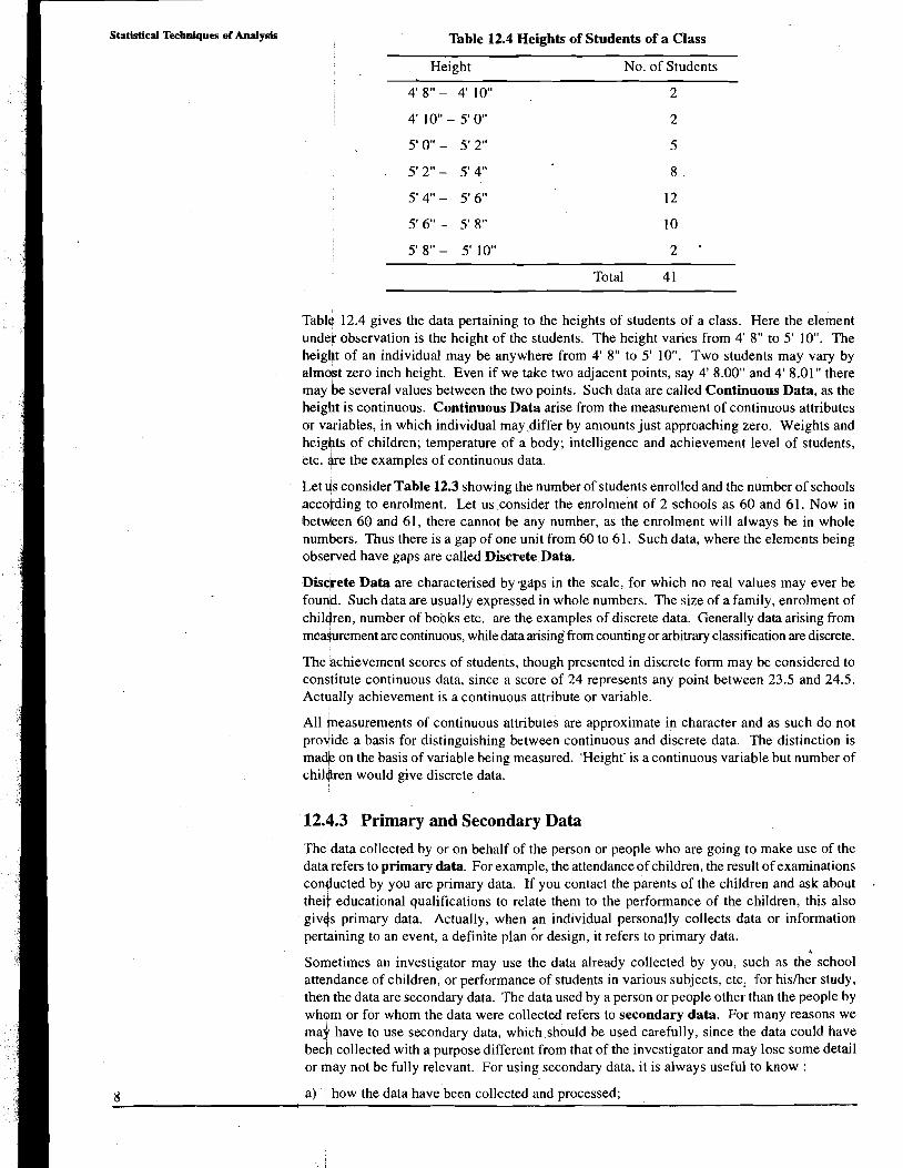
T,et us consider the Table 12.4 depicting the heights of students of a class.

Statistical Tezhniques of Analysis Table 12.4 Heights of Students of a Class

Height No. of Students

4 '8"- 4' 10" 2

5 ' 8 " - 5'10" 2 *

Total 4 1

Tablq 12.4 gives the data pertaining to the heights of students of a class. Here the element under observation is the height of the students. The height varies from 4' 8" to 5' 10". The height of an individual may be anywhere from 4' 8" to 5' 10". Two students may vary by almost zero inch height. Even if we take two adjacent points, say 4' 8.00" and 4' 8.01" there may be several values between the two points. Such data are called Continuous Data, as the heigbt is continuous. Continuous Data arise from the measurement of continuous attributes or vdriables, in which individual may differ by amounts just approaching zero. Weights and heig$ts of children; temperature of a body; intelligence and achievement level of students, etc. are the examples of continuous data.

Let ds consider Table 12.3 showing the number of students enrolled and the number of schools accotding to enrolment. Let us,consider the enrolment of 2 schools as 60 and 61. Now in betdeen 60 and 61, there cannot be any number, as the enrolment will always be in whole numbers. Thus there is a gap of one unit from 60 to 61. Such data, where the elements being observed have gaps are called Discrete Data.

Discbete Data are characterised by ,gilps in the scale, for which no real values may ever be found. Such data are usually expressed in whole numbers. The size of a family, enrolment of children, number of books etc. are the examples of discrete data. Generally data arising from meagurement are continuous, while data arising from counting or arbitrary classification are discrete.

The achievement scores of students, though presented in discrete form may be considered to constitute continuous data, since a score of 24 represents any point between 23.5 and 24.5. Actually achievement is a continuous attribute or variable.

All peasurements of continuous attributes are approximate in character and as such do not prodide a basis for distinguishing between continuous and discrete data. The distinction is madie on the basis of variable being measured. 'Height' is a continuous variable but number of chilqren would give discrete data.

12.4.3 Primary and Secondary Data

The data collected by or on behalf of the person or people who are going to make use of the data refers to primary data. For example, the attendance of children, the result of examinations conducted by you are primary data. If you contact the parents of the children and ask about theit. educational qualifications to relate them to the performance of the children, this also give+ primary data. Actually, when an individual personally collects data or information per$ining to an event, a definite plan or design, it refers to primary data.

* Sodetimes an investigator may use the data already collected by you, such as the school attehdance of children, or performance of students in various subjects. etc, for hislher study, the9 the data are secondary data. The data used by a person or people other than the people by whom or for whom the data were collected refers to secondary data. For many reasons we may have to use secondary data, which should be used carefully, since the data could have beeh collected with a purpose different from that of the investigator and may lose some detail or may not be fully relevant. For using secondary data, it is always useful to know :

d a) how the data have been collected and processed;

b) the accuracy of data; TalmhtionradGrppllicaS * RepEwaIalim d Data

' c.) how far the data have been summarised;

d) how comparable the data are with other tabulations; and

e) how to interpret the data, especially when figures collected for one purpose are used for another purpose. -- " .- _ I.l-." -L---------.-p-IIII------̂ I1 -- ~ I L < b 1 , & I ! > 1 ( * > 5 , \ ~ ~

12.5 MEASUREMENT SCALES

Measurement refers to the assignment of numbers to objects and events according to logical acceptable rules. The numbers have many properties, such as identity, order and additivity. If we can legitimately assign numbers in the describing of objects and events, then the properties of numbers should be applicable to the objects and events. It is essential to know about the

I different kinds of measurement scales, as the number of properties applicable depends upon the measurement scale applied to the objects or events.

Let us take four different situations for a class of 30 students :

.-- assigning them roll nos. from 1 to 30 on random basis.

- asking the students to stand in a queue as per their heights and assigning them position numbers in queue from 1 to 30.

- administering a test of 50 marks to all students and awarding marks from 0 to 50, as per their performance.

- measuring the height and weight of students and making student-wise record.

In the first situation, the numbers have been assigned purely on arbitrary basis. Any student could be assigned No. 1 while any one could be assigned No. 30. No two students can be compared on the basis of allotment of numbers, in any respect. The students have been Iaklled

Statistical Techniques of Analysis from 1 to 30 in order to give each an identity. This scale refers to nominal scale. Here the property of identity is applicable but the properties of order and additivity are not applicable.

In the second situation, the students have been assigned their position numbers in queue from 1 to 30. Here the numbering is not on arbitrary basis. The numbers have been assigned acco~ding to the height of the students. So the students are comparable on the basis of their heights, as there is a sequence in this regard. Every subsequent child is taller than the previous one, and so on. This scale refers to ordinal scale. Here the object or event has got its identity, as well as order. As lhe difference in height of any two students is not known, so the property of addition of numbers is not applicable to the ordinal scale.

In the third situation, the students have been awarded marks from 0 to 50 on the basis of their performance in the test administered on them. Consider the marks obtained by 3 students, which are 30,20 and 40 respectively. Here, it may be interpreted that the difference between the performance of the 1st and 2nd student is the same, as between the performance of the 1st and the 3rd student. However, no one can say that the performance of the 3rd student is just the double of the 2nd student. This is because there is no absolute zero and a student getting 0 marks, cannot be termed as having zero achievement level. This scale refers to interval scale. Here the properties of identity, order and additivity are applicable.

In the fourth situation, the exact physical values pertaining to the heights and weights of all students have been obtained. Here the values are comparable in all respect. If two students have heights of 120 cm and 140 cm, then the difference in their heights is 20 cm and the heights are in the ratio 6:7. This scale refers to ratio scale.

4. l'oint 6:)uc. \vhii.h ol' l t ) ~ : i'ollr. mi.;aui-cl~rcnl sc;tlcs IS i:'~!i~ ~lscc! in t i , : j:li:.t:+:!r!:: ;..<;il;il~,ic.;:

12.6 MEANING OF STATISTICS

In order to understand the meaning of statistics a few definitions are stated below :

a) Scatistics can be described as the science of classifying and organising data in order to draw inferences.

b) Smtistics refers to the methodology for the collection, presentation and analyses of data and for the uses of such data.

C) St~ftistics is concerned with scientific methods for collecting, organising, summarising, presenting and analysing data, as well as drawing valid concl~lsions and making reasonable dqcisions on the basis of this analysis. It is concerned with the systematic collection of n~tmerical data and its interpretation. This systematic collection of data distinguishes statistics from other kinds of information.

d) Sthtistics is the science which helps us to extract useful information for numerical data. It does not restrict itself to the collection and presentation of data, but it also deals with the interpretation and drawing of inferences from the data.

The tern statistics is used both in its singular and plural sense. In the singular sense, it is a science which concerns itself with the collection, presentation and drawing of conclusions

10 from nomerical data. In the plural sense, it means numerical facts or observations collected

with a definite object in view. Statistics are expressed quantitatively and not qualitatively. lsbulptian and Grpphieal Repreentation of Data

12.7 NEED AND IMPORTANCE OF STATISTICS

Any learned person likes to read the literature in hislher field. Even a teacher has to read a lot. While going through this literature, one comes across statistical symbols, concepts and ideas. A study of statistics helps one to draw one's own conclusions from them rather than accepting the writer's inferences. As a teacher, you have to use tests and other tools for assessing the achievement level and other behaviour of the children. With the help of simple stat.istica1

. methods interpretation of scores becomes much more meaningful. If a teacher is interested in understanding research work, he needs more extensive skills in statistical methods.

The language of mathematics and statistics permits the most exact kind of description. These disciplines also force us to be definite and exact in our procedures and in our thinking. Statistics enable us to summarise our results in meaningful and convenient form. They enable us to draw general conclusions according to accepted rules and say to what extent faith should be placed in such generalisations. Under conditions we know and have measured, statistics enables us to predict, what is likely to happen. It also enables us to analyse some of the causal factors of complex events. r--- -' '

i 1 Check 'rbur Prcrgress i 5 , *-.+., ,L ~ u o such situations where statistics can be u:;cf'ui.

.............................................................................................................................. i

.............................................................................................................................. 1 ............................. t .............................................................................................. ..;

i

/ ................................................. " ........ . . . . . .................................................... I

12.8 IMPORTANCE OF THE ORGANISATION OF DATA

'Nhen a set of data contains only a few entries, a simple listing of the observations might be sufficient for interpreting the data. But usually in our schools, the number of children in a class is large, so the simple listing of the observations may not be sufficient for the interpretation of data pertaining to the entire class. Here the data are usually organized into groups called classes and presented in a table which gives the number of observations in each group. Such a table gives a better overall view of the distribution of data and enables one to rapidly assess important characteristics of the data.

'The simplest way to organise a set of data is to present the data in a sequence. Even when data contains only a few entries, presenting it in a sequence, makes it easy to comprehend and interpret. For example, let us consider the height of 15 childrens as shown below :

Height in cms : 142,156,139,148,150,149,148,144,150,152,148,149,147,141 and 145. Little can be said about the height of the children from these figures. Even if you make an effort you will find yourself re-arranging them in some way. For example, you may be looking for the minimum and the maximum figures or the number that is most frequent.

Yow arrange these heights in a sequence from lowest to highest.

Height incms: 139,141,142,144,145,147,148,148,148,149,149,150,150,152and 156. Even after a cursory look at the arranged data, one can say that the height of the children varies from 139 cm to 156 cm: there are 3 children having the same height of 148 cm and the number of children having height below 148 cm and having height above 148 cm is the same. Similarly, one can immediately respond to the number of children upto a specified height and SO on.

Statistical Techniques of Analysis Data can be arranged in two ways. One, from lowest to highest referred to as the ascending order, and the other, from highest to lowest referred to as the descending order of presentation.

Check \'our Progress

0 . .41Laryo 111c 1u:lrks of20 stutlcl~ls In English lanf.u~lgc in i ~ s i c ~ ~ c l i ~ ~ g orc1c.r LIIIL! ; I I I V ~ C I Ilic Iollol&ing qucslionh.

hl:lrks in English Larlguapc :

( 3 5 . 18. 39. 57. 70. 49. 33. 72 . 6 1 . 32. 3s . 66. 75. 5 7 . i. 59. (70. 47. 55. 0 s .

12.10 GROUPING AND TABULATION OF DATA It is cumbersome to study or interpret large data without grouping it, even if it is arranged sequentiqlly. For this, the data are usually organised into groups called classes and presented in a table which gives the frequency in each group. Such a frequency table gives a better overall view of the distribution of data and enables a person to rapidly comprehend important characteristics of the data.

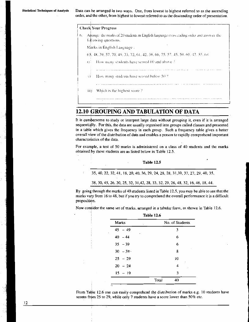
For example, a test of 50 marks is administered on a class of 40 students and the marks obtained by these students are as listed below in Table 12.5.

Table 12.5

By going through the marks of 40 students listed in Table 12.5, you may be able to see that the marks vary from 16 to 48, but if you try to comprehend the overall performance it is a difficult propositibn.

I

Now conbider the same set of marks, arranged in a tabular form, as shown in Table 12.6.

Table 12.6

Marks No. of Students

45 - 49 3

Total 40

From Table 12.6 one can easily comprehend the distribution of marks e.g. 10 students have scores fr+m 25 to 29, while only 7 students have a score lower than 50% etc.

12

Yarious terms related to the tabulation of data are being discussed below : Tabulatkm and Graphid Representation of Data

Table 12.6'shows the marks arranged in descending order of magnitude and their corresponding frequencies. Such a table is known as frequency distribution. A grouped frequency distribution has a minimum of two columns - the first has the classes arranged in some meaningful order, and a second has the corresponding frequencies. The classes are also referred to as class intervals. The range of scores or values in each class interval is the same. In the given example the first class interval is from 45 to 49 having a range of 5 marks i.e. 45,46,47, 48, and 49. Here 45 is the lower class limit and 49 is the upper class limit. As discussed earlier the score of 45 may be anywhere from 44.5 to 45.5, so the exact lower class limit is 44.5 instead of 45. Similarly, the exact upper class limit is 49.5 instead of 49. The range of the class interval is 49.5 - 44.5 = 5 i s . the difference between the upper limit of class interval and the lower limit of class interval.

For the presentation of data in the form of a frequency distribution for grouped data, a number of steps are required. These steps are :

1. Selection of non-overlapping classes.

2. Enumeration of data values that fall in each class.

3 . Construction of the table.

Let us consider the score of 120 students of class X of a school in Mathematics, shown in Table 12.7.

Table 12.7 Mathematics score of 120 class X Students

71 8541889845756681 3852679262834964529061586391 5748 75 89736480677665766561 68 84725777635256416055755345 3791 5740736676528862786855673965444758684290893969 488291 398544716856489044624783 80966988244438749339 725646718046547758 817058 5178648450958759

First we have to decide about the number of classes. We usfially-have 6 to 20 classes of equal length. If the number of scores/events is quite large, we usually have 10 to 20 classes. The number of classes when less than 10 is considered only when the number of scoreslvalues is not too large. For deciding the exactaumber of classes to.be taken, we have to find out the range of scores. In Table 12.7 scores vary from 37 to 98 so the range of the score is 62 (98.5 - 36.5 = 62).

'i'he length of class interval preferred is 2, 3, 5, 10 and 20. Here if we,take class length of 10 ~llen the number of class intervals will be 62/10 = 6.2 or 7 which is less than the desired rumber of classes. If we take class length of 5 then the number of class intervals will be (1215 = 12.4 or 13 which is desirable.

Now, where to start the first class interval ? The highest score of 98is included in each of the three class intervals of length 5 i.e. 94 - 98,95 - 99 and 96 - 100. We choose the interval 95 - 99 as the score 95 is multiple of 5. So the 13 classes will be 95 - 99,90 - 94, 85 - 89, 80 - 84, . . . . . . . , 35 - 39. Here, we have two advantages. One, the mid points of the classes are whole numbers, which sometimes you will have to use. Second, when we start with the multiple of the lengih of class interval, it is easier to mark tallies. When the size of class interval is 5, we start with 0, 5, 10, 15, 20 etc.

'To know about these advantages, you may try the other combinations also e.g. 94 -98, 89 - 93, 84 - 88, 79 -83 etc. You will observe that marking tallies in such classes is a bit more difficult. You may also take the size of the class interval as 4. There you will observe that the mid points are not whole numbers. So, while selecting the size of the class interval and the limits of the classes, one has to be careful.

After writing the 13 class intervals in descending order and putting tallies against the concerned class interval for each of the scores, we present the' frequency distribution as shown in Table 12.8.

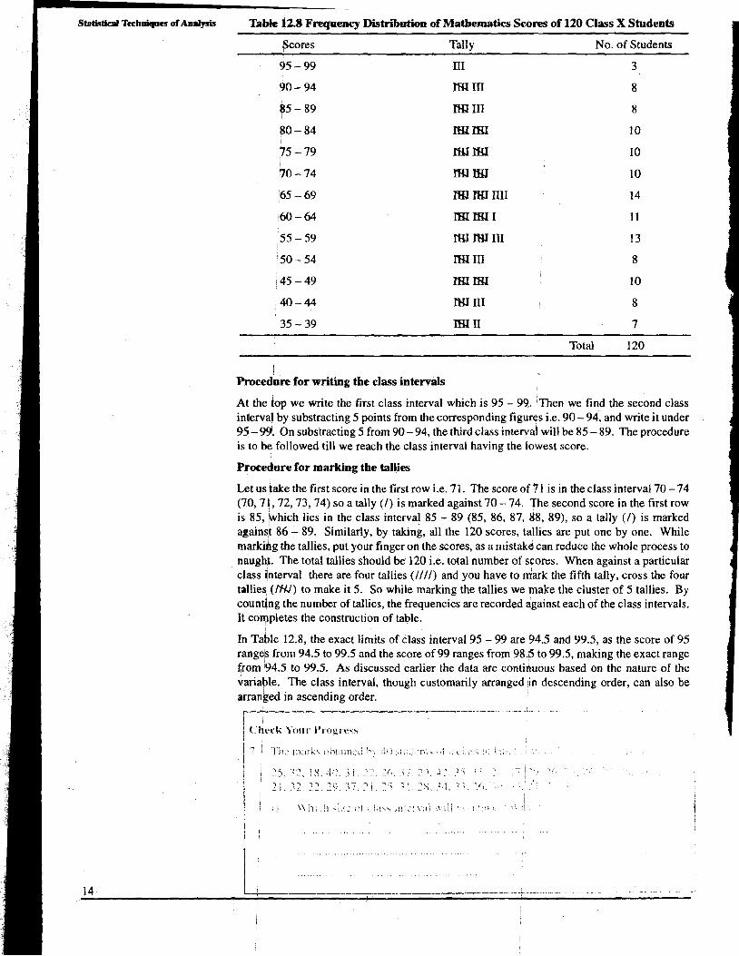
St~thtacJII Tcrhnigocs ofbe- Table 12.8 Frequency Distriition of Matbematics Scores of 120 Class X Students

Scores -- -

Tallv No. of Students

35 - 39 WI I1 7

Total 120

Procedbre for writing the class intervals I

At the top we write the first class interval which is 95 - 99. Then we find the second class interval by substracting 5 points from the corresponding figures i.e. 90 - 94, and write it under 95- 991. On substracting 5 from 90- 94, the third class interval will be 85 - 89. The procedure is to be followed till we reach the class interval having the lowest score.

Procedure for marking the tallies

Let us take the first score in the first row i.e. 71. The score of 7 1 is in the class interval 70 -74 (70,7 1,72,73,74) so a tally ( I ) is marked against 70 - 74. The second score in the first row is 85, bvhich lies in the class interval 85 - 89 (85, 86, 87, 48, 89), so a tally (1) is marked againsk 86 - 89. Similarly, by taking, all the 120 scores, tallies are put one by one. While rnarkihg the tallies, put your finger on the scores, as a mistake can reduce the whole process to naughlt. The total tallies should be 120 i.e. total number of scores. When against a particular class interval there are four tallies ( I / / / ) and you have to mark the fifth tally, cross the four tallies (MV) to make it 5. So while marking the tallies we make the cluster of 5 tallies. By cbundng the number of tallies, the frequencies are recorded against each of the class intervals. It completes the construction of table.

In able 12.8, the exact limits of class interval 95 - 99 are 94.5 and 99.5, as the score of 95 rangep from 94.5 to 99.5 and the score of 99 ranges from 98.5 to 99.5, making the exact range from (94.5 to 99.5. As discussed earlier the data are contihuous based on the nature of the variable. The class interval, though customarily arranged in descending order, can also be arranged in ascending order.

r'--- --.-------. + - " "

i ! I ! i ! . : : i . ! ~ ~ , ;!1,3 L I ! ~ . C . : I L ! ~ L I : ~ . ,?\chi ~ I I C I ' ~ C ~ L I C I I Z ~ ; ~ n d Z I I C ' C ~ tli;~t ~ h c total is 40. 1f ! : :lii r ;~ . : . i< ;! !n~,.!:il\t.. rs! to ~ l ! i n l \ u:h,\r p l . c c ; ~ u ~ i o n \ y o u xhonlcl l l ~ ? \ ' c l a k t n and i .It, i t ttc:~in. i I'I.!, X I ! .ou~- o\cn I i I

12.11 GRAPHICAL REPRESENTATION OF DATA

The data which has been shown in the tabular form, may be displayed in pictorial form by using a graph. A well-constructed graphical presentation is the easiest way to depict a given set of data.

Tabulation and Graphical Representalion of Data

12.12 TYPES OF GRAPHICAL REPRESENTATION OF DATA

Here only a few of the standard graphic forms of representing the data are being discushed as listed below :

a Histogram

a Bar Diagram or Bar Graph

a Frequency Polygon

a Cumulative Frequency ~ u & e or Ogive

12.12.1 Histogram

The most common form of graphical presentation of data is histogram. For plotting a histogram, one has to take a graph paper. The values of the variable are taken on the horizontal axislscale known as X-axis and the frequencies are taken on the vertical axislscale known as Y-axis. For each class interval a rectangle is drawn with the base equal to the length of the class interval and height according to the frequency of the C.I. When C.I. are of equal length, which would generally be the case in the type of data you are likely to handle in school situations, the heights of rectangles must be proportional to the frequencies of the Class Intervals. When the C.I. are not of equal length, the areas of rectangles must be proportional to the frequencies indicated (most likely you will not face this type of situation). As the C.1.s for any variable are in continuity, the base of the rectangles also extends from one boundary to the other in continuity. These boundaries of the C.1.s are indicated on the horizontal scale. The frequencies for determining the heights of the rectangles are indicated on the vertical scale of the graph.

Let us prepare a histogram for the frequency distribution of mathematics score of 120 Class X students (Table 12.8).

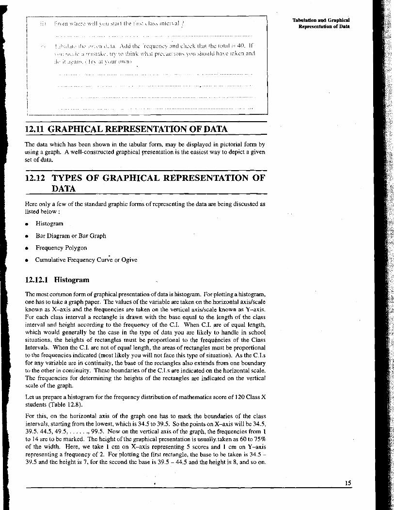
For this, on the horizontal axis of the graph one has to mark the boundaries of the class intervals, starting from the lowest, which is 34.5 to 39.5. So the points on X-axis will be 34.5, 39.5, 44.5, 49.5, . . . . . . . 99.5. Now on the vertical axis of the graph, the frequencies from 1 to 14 are to be marked. The height of the graphical presentation is usually.taken as 60 to 75% of the width. Here, we take 1 cm on X-axis representing 5 scores and 1 cm on Y-axis representing a frequency of 2. For plotting the first rectangle, the base to be taken is 34.5 - 39.5 and the height is 7, for the second the base is 39.5 - 44.5 and the height is 8, and so on.

Statistical Techniqws of Analysis The histogram will be as shown in Figure 12.1.

Scores

Fig. 12.1: Distribution of Mathematics Scores

Let us re-group the data of Table 12.8 by having the length of class intervals as 10, as shown in Table 12.9.

Table 12.9 Frequency Distribution of Mathematics Scores - -- -- - - - - - - -

Scores Frequency

90 - 99 11 80 - 89 18 70 - 79 20 60 - 69 25 50 - 59 2 1 48 - 49 18 30 - 39 7

Total 120

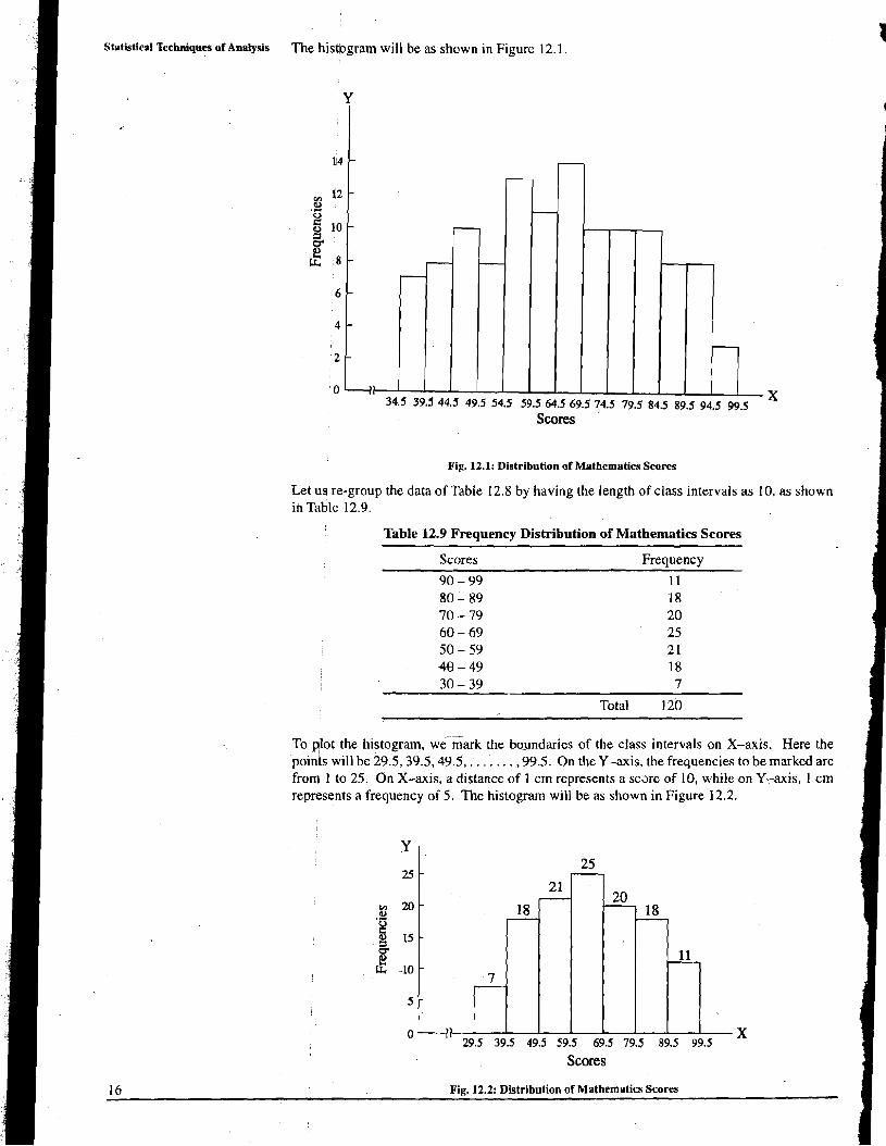
To plot the histogram, we-mark the boundaries of the class intervals on X-axis. Here the poinp will be 29.5,39.5,49.5,. . .-. . . . ,99.5. On they-axis, the frequencies to be marked are from 1 to 25. On X-axis, a distance of 1 cm represents a scare of 10, while on Y-axis, 1 cm represents a frequency of 5. The histogram will be as shown in Figure 12.2.

Scores

16 Fig. 12.2: Distribution of Mathematics Scores

If we observe Figures 12.1 and 12.2, we find that figure 12.2 is simpler than Figure 12.1. Tabulation and G r a p h i d Representation of Data

Figure 12.1 is complex because the number of class intervals is more. If we further increase - the number of class intervals, the figure obtained will be still more complex. So for plotting the histogram for a given data, usually we prefer to have less number of class intervals.

12.12.2 Bar Diagram or Bar Graph

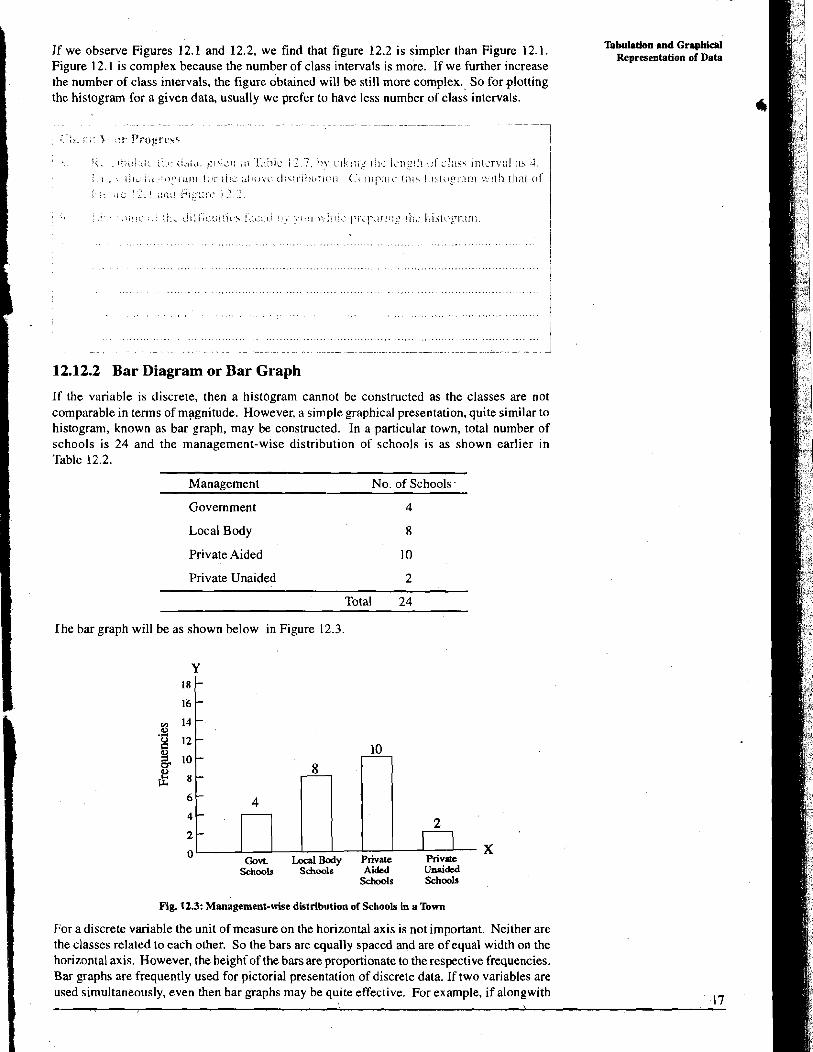
If the variable is discrete, then a histogram cannot be constructed as the classes are not comparable in terms of magnitude. However, a simple graphical presentation, quite similar to histogram, known as bar graph, may be constructed. In a particular town, total number of schools is 24 and the management-wise distribution of schools is as shown earlier in Table 12.2.

Management No. of Schools.

Government 4

Local Body 8

Private Aided 10

Private Unaided - -

Total 24

The bar graph will be as shown below in Figure 12.3.

u Govr Local Body Private Private Schools Schmls Aided Unaidcd

Schools Schools

1 Fig. 12.3: Management-wise distribution of Schools in a Town

For a discrete variable the unit of measure on the horizontal axis is not important. Neither are 1 the classes related to each other. So the bars arc equally spaced and are of equal width on the I horizontal axis. However, the height of the bars are proportionate to the respective frequencies.

Bar graphs are frequently used for pictorial presentation of discrete data. If two variables are used simultaneously, even then bar graphs may be quite effective. For example, if alongwith - 17

\

Statistical Techniques of Analysis the total number of schools (management-wise) the number of boys' schools, girls' schools and co-ed schools are also to be indicated then this can be done on the same graph paper by using different colours, each indicating the sex-wise category. For each management there will be 4 bars having different colours indicating different categories.

12.124 Frequency Polygon

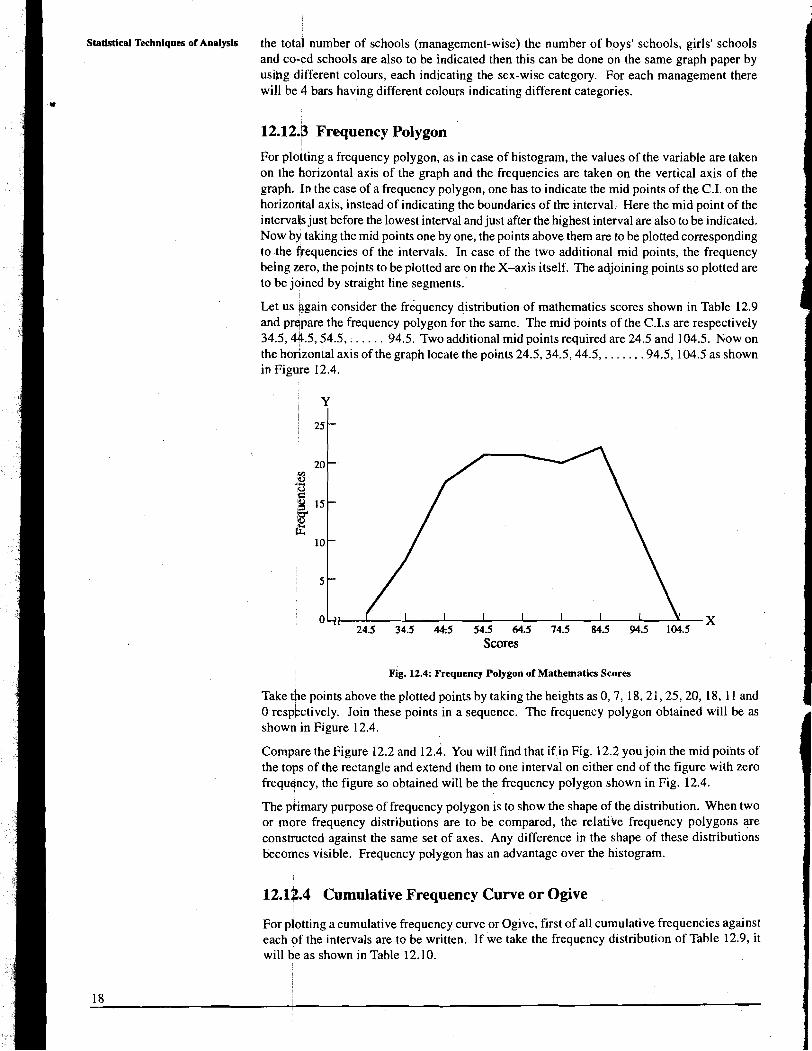
For plotting a frequency polygon, as in case of histogram, the values of the variable are taken on the horizontal axis of the graph and the frequencies are taken on the vertical axis of the graph. In the case of a frequency polygon, one has to indicate the mid points of the C.I. on the horizontal axis, instead of indicating the boundaries of the interval, Here the mid point of the intervals just before the lowest interval and just after the highest interval are also to be indicated. Now by taking the mid points one by one, the points above them are to be plotted corresponding to the frequencies of the intervals. In case of the two additional mid points, the frequency being zero, the points to be plotted are on the X-axis itself. The adjoining points so plotted are to be jained by straight line segments.

Let us @gain consider the frequency distribution of mathematics scores shown in Table 12.9 and prelpare the frequency polygon for the same. The mid points of the C.1.s are respectively 34.5,44.5,54.5, . . . . . . 94.5. Two additional mid points required are 24.5 and 104.5. Now on the horizontal axis of the graph locate the points 24.5,34.5,44.5, . . . . . . .94.5, 104.5 as shown in Figure 12.4.

Scores

Fig. 12.4: Frequency Polygon of Mathematics Scores

Take the points above the plotted points by taking the heights as 0,7, 18,21,25,20, 18, 11 and 0 respectively. Join these points in a sequence. The frequency polygon obtained will be as showd in Figure 12.4.

Comp~re the Figure 12.2 and 12.4. You will find that if in Fig. 12.2 you join the mid points of the tops of the rectangle and extend them to one interval on either end of the figure with zero frequqncy, the figure so obtained will be the frequency polygon shown in Fig. 12.4.

The ptimary purpose of frequency polygon is to show the shape of the distribution. When two or more frequency distributions are to be compared, the relatiCe frequency polygons are consthcted against the same set of axes. Any difference in the shape of these distributions becomes visible. Frequency polygon has an advantage over the histogram.

12.12.4 Cumulative Frequency Curve or Ogive

For plotting a cumulative frequency curve or Ogive, first of all cumulative frequencies against each pf the intervals are to be written. If we take the frequency distribution of Table 12.9, it will he as shown in Table 12.10.

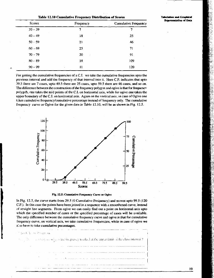
Table 12.10 Cumnlative Frequency Distribution of Scores ~ a b u ~ o m p a d ~ ~ -0aobD.t.

Scores Frequency Cumulative Frequency

For getting the cumulative frequencies of a C.I. we take the cumulative frequencies upto the previous interval and add the frequency of that interval into it. Here C.F. indicates that upto 39.5 there are 7 cases, upto 49.5 there are 25 cases, upto 59.5 there are 46 cases, and so on. The difference between the construction of the frequency polygon and ogive is that for frequerw~ polygoh, one takes the mid points of the C.I. on horizontal axis, while for ogive one takes the upper boundary of the C.I. on horizontal axis. Again on the vertical axis, in case of Ogive one tzkes cumulative frequency/cumulative percentage instead of frequency only. The cumulative frequency curve or Ogive for the given data in Table 12.10, will be as shown in Fig. 12.5.

Fig. 12.5: Cumulative Frequency Curve ar W v e

In Fig. 12.5, the curve starts from 29.5 (0 Cumulative Frequency) and moves upto 99.5 (120 C.F.). In this case the points have been joined in a sequence with a smoothened cwve, instead of straight line segments. From ogive we can easily find out a point on horizontal axis upto which the specified number of cases or the specified percentage of cases will be available. The only difference between the cumulative frequency curve and ogive is that for cumulative frequency curve, on vertical axis, we take cumulative frequencies, while in case of ogive we a:so have to take cumulative percentages.

, : : < ;.; . t , 1 ... :&. . .... < .. 14 . .

. . ;:!.., I ;I:..: iiC.j:cii, i. ~;::l.;hl.:~i :it I!:C 11J7['cl [ i l l 1 1 1 : , i t I : ~ L ' ~ ; L S S llllcl.\;fl1 '? , ,. ,

I

Statistical Techniques of Analysis 12.13 LET US SUM UP

Data refers .to the set of observations, value, elements or objects under consideration.

Data may be either qualitative or quantitative; it may be either continuous or discrete; or it may be either primary or secondary, depending on the nature of elements.

Elements classified into categories yield qualitative data, while the elements in the form of number yield quantitative data.

The data used by an investigator is primary if it has been collected by him or for him. If the data used is not collected by him or for him then it is secondary.

There are four type of measurement scales, namely nominal, ordinal, interval and ratio scales. The operations to be performed on measurements depend upon the type of measurement scale used.

Sdection of non-overlapping classes; enumeration of data values in each class; and the co~nstruction of table, are the three steps required for the preparation of frequency distribution.

Ahy qualitative data may be represented by Bar Diagram or Bar Graph, while the quantitative data may be represented by Histogram, or Frequency Polygon, or Cumulative Frequency Curve or Ogive.

12.14 UNIT-END EXERCISES

1. Collect two sets of observations, one of them qualitative and the other one quantitative. Ptesent these observations in tabular form.

2. Administer a test in your class. Classify the data so obtained, in the form of a frequency distribution.

.......................................................................................................................................... 3. Suitably represent the two sets of observations and the test result by graphical presentation.

12.15 POINTS FOR DISCUSSION

1 . In your daily life situations or in the newspaper, you come across a number of sets of data. , Note down the same in the exercise book alongwith the nature of each set of data. Discuss

20 it with your tutor/counsellor. -

2. In your classroom, you administer a number of tests. Classify the dataof each test in the Tabadatloo and Graphid

form of a frequency distribution. There you may face a problem in selecting the non- Representation of Data

overlapping classes, the same may be discussed with the tutor/counsellor.

3. Try to classify any given data into a number of frequency distributions by taking different class intervals. Identify the best classification and discuss it with the tutor/counsellor.

12.16 ANSWERS TO CHECK YOUR PROGRESS

1. i) Qualitative Data (Here the attendance has been given class-wise, so it refers to class as a category. If the classes would have been identifiedcategorised according to the attendance, then it would have become quantitative data).

ii) Quantitative Data

2. i) Continuous Data

3. i)

ii)

4. i)

ii)

iii)

i v)

5. a)

b)

6. i)

i i)

iii)

7. i)

Continuous Data (Here the scores obtained will be in whole numbers, but the spelling ability is continuous in nature).

Secondary Data

Primary Data

Ratio Scale

Nominal Scale

Ordinal Scale

Interval Scale

Interpreting the score obtained from various tests administered to students.

Drawing general conclusion on achievement of students according to accepted rules.

3 (The scores vary from 15 to 42, so the range of the score is 42.5 -14.5 = 28. Thus, if the size of the class interval is taken as 3, the number of classes will be 10, which is an appropriate number).

ii) 42 - 44 representing 41.5 - 44.5 will be the first class interval.

12.17 SUGGESTED READINGS

Garrett, H.E. (1956), Elementary Statistics, Longmans, Green & Co., New York. I

i Guilford, J.P. (1965), Fundamental Statistics in Psychology and Education, Mc Graw Hill

i Book Company, New York.

Hannagan, T.J. (1982), Mastering Statistics, The Macmillan Press Ltd., Surrey. I

Jaeger, R.M. (1983), Statistics : A Spectator Sport, Sage Publications India Pvt. Ltd., New Delhi.

I Lindgren, B.W. (1975), Basic Ideas of Statistics, Macmillan Publishing Co. Inc., New York.

Walker, H.M. and Lev, J. (1965), Elementary Statistical Methods, Oxford & IBH Publishing Co., Calcutia.

Wine. R.L. (1976), Beginning Statistics, Winthrop Publishers Inc., Massachusetts.