2936-trt cable chauffant.pdf

Proceedings World Geothermal Congress 2010 Bali, Indonesia, 25-29 April 2010

1

A Novel Thermal Response Test Using Heating Cables

J. Raymond1, G. Robert1, R. Therrien1 and L. Gosselin2

1Département de géologie et de génie géologique, 2Département de génie mécanique, Université Laval, 1065 avenue de la médecine, Québec (Qc), G1V 0A6, Canada

[email protected]; [email protected]; [email protected]; [email protected]

Keywords: heat pump, heat exchanger, thermal response test, heating cable, thermal conductivity

ABSTRACT

The in situ thermal conductivity of the subsurface has been measured with a novel thermal response test using heating cables inserted in a vertical ground heat exchanger. An electric current is applied along the cables to heat the borehole prior to measuring water temperature recovery at various depths inside the ground heat exchanger piping. The one-dimensional line-source equation, combined with the superposition principle accounting for the recovery period, is used to reproduce temperature measurements by adjusting the thermal properties of the subsurface. The adjusted subsurface thermal conductivity is independent of the borehole thermal resistance because the latter parameter is eliminated form the analytical solution describing temperature recovery. The analysis of the thermal response test can alternatively be performed with two- or three-dimensional numerical models to account for spatially-distributed heterogeneities of the subsurface, ambient groundwater flow and the geothermal gradient. The advantages of the heating cable test compared to conventional thermal response tests are that heat flow to the borehole is more constant and uniform because the heat source is located along the borehole and it is not affected by temperature changes at ground surface, the equipment required is more compact and easily installed, and the test can be fully automated to reduce time spent in the field. The test can also be conducted on any type of borehole, allowing investigation of in situ thermal properties when boreholes are drilled but ground heat exchangers are not installed.

1. INTRODUCTION

In situ thermal response tests, also called borehole thermal conductivity tests, are conducted to measure thermal properties of both the subsurface and boreholes to design ground-coupled heat pump systems. The conventional testing method consists in reproducing heat transfer that would occur in a vertical ground heat exchanger by circulating water that is heated with an electric element in a close loop (ASHRAE, 2007; Sanner et al., 2005). Water temperatures are measured at the inlet and the outlet of the ground heat exchanger along with flow rate. The borehole temperature increments observed during the heating period is interpreted using analytical or numerical models to determine the subsurface and the borehole thermal parameters (Gehlin and Hellström, 2003). The test has been particularly useful for commercial system design where the parameters measured are used to size ground heat exchangers. The conventional testing method is however expensive because it requires mobilization of heavy equipment. Handling of the equipment in the field is also arduous. Water reservoirs and piping must be handled with care to avoid leaks. Piping should be well insulated to minimize heat transfer with the surface environment.

An alternative testing method that is easier to perform has been developed to conduct TRT. The method is based on the work of Pehme et al. (2007a; b), who measured in situ subsurface thermal properties using heating cables inserted in water filled boreholes and it is adapted for ground heat exchangers. The testing methodology and the analysis of data are detailed below and results of two tests are reported. The new method is finally compared to conventional TRTs that use flowing water.

2. TEST METHODOLOGY

Heating cables are lowered in pipes of the ground heat exchanger after its installation. Cables can be inserted in each tube of the U-pipe exchanger or in the inner tube of a concentric exchanger. Tests, such as those conducted by Pehme et al. (2007a; b), can also be performed in a borehole where the ground heat exchanger has not been installed by lowering the cables in the borehole where the well screen has been either blocked or left open. Heat dissipated by each cable is a function of its electrical resistance, which can vary slightly with temperature. The cables used for the tests reported here had a resistance of 37.0 Ω at 20 C and a length of 24.38m. The resistance of the cables was determined for the range of temperatures expected during the tests (Appendix 1). Sensors are placed along the cables to measure temperature at fixed depths. Thermistors were used in this study, but other sensors such as optical fibers (Hurtig et al., 1994; Hurtig et al., 1996) could also be used to increase the number of measurement points. A data logger, located at surface in the testing unit, records temperature. The data logger is connected to the thermistors with electric cables. The electrical tension induced in the heating cable was measured and recorded with a variable transformer and a data logger equipped with a voltmeter. The transformer was calibrated prior to field measurements (Appendix 1). Heat dissipation per unit length of cable, q [MLt-3], is calculated from voltage measurements, Ф [L2Mt-3C-1], using Joule’s and Ohm’s law:

LRqe

2Φ= (1)

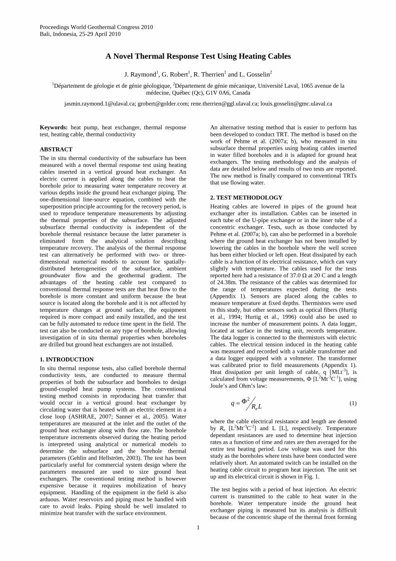
where the cable electrical resistance and length are denoted by Re [L2Mt-3C-2] and L [L], respectively. Temperature dependant resistances are used to determine heat injection rates as a function of time and rates are then averaged for the entire test heating period. Low voltage was used for this study as the boreholes where tests have been conducted were relatively short. An automated switch can be installed on the heating cable circuit to program heat injection. The unit set up and its electrical circuit is shown in Fig. 1.

The test begins with a period of heat injection. An electric current is transmitted to the cable to heat water in the borehole. Water temperature inside the ground heat exchanger piping is measured but its analysis is difficult because of the concentric shape of the thermal front forming

Raymond et al.

2

around the cables. Noise can be induced by movement of the cable and tied sensors standing in the pipe water. Pehme et al. (2007a; b) could analyze temperature measured during the heating period as their tests were performed in water filled boreholes where the cables stand in a cylinder of larger diameter that is in direct contact to the host rock. Temperature measured during the heating period is however very difficult to analyze when tests are conducted in ground heat exchangers because the cables stand in a cylinder of smaller diameter (the U-pipe) that has a low thermal conductivity. The pipe slows down the progression of the thermal front, increasing the thermal gradient such that a small movement of the cable located in a zone of concentric gradient can induce significant noise. Temperature data is used during the heating period to determine the values of electrical resistance required to compute the heat injection rate. The duration of the heating period depends on the desired radius of influence and can be estimated with the line-source equation, as shown in the next section.

Figure 1: Thermal response test unit with heating cables

The next step of the TRT is to stop heat injection and then measure temperature recovery in the ground heat exchanger. The temperature can be measured until it is sufficiently close to the undisturbed subsurface temperature. Measurements can be conducted in each tube of the U-pipe ground heat exchanger and are averaged for a given depth. One measurement point per given depth is however sufficient for a concentric ground heat exchanger because the exchanger is symmetrical. Temperature inside the ground heat exchanger homogenizes rapidly during the recovery period. The recorded temperature signal is consequently smooth even if the cable moves and temperature can be analyzed easily to determine the subsurface thermal properties using analytical or numerical models.

3. TEST ANALYSIS

Models are used to reproduce temperature signals recorded at given depths during the recovery period. Computed temperatures are fitted to observed temperatures to determine the subsurface thermal conductivity with depth. Analytical models such as the cylindrical- or the line-source (Carslaw, 1945; Ingersoll et al., 1954) can be used for tests conducted with heating cables. A numerical model can also

be used and additionally account for other phenomena not considered in analytical solutions such as spatially-distributed subsurface heterogeneities, groundwater flow and the geothermal gradient. The line-source model has been used in this study and its application is described below, followed by numerical analysis techniques.

3.1 The Line-Source Model

The analytical solution is derived from Kelvin’s line-source equation that describes the mean temperature increment ∆T at a radial distance r [L] from an infinite linear source of heat having a constant heat flow rate according to:

duu

eqtrT

u

u

∫∞ −

=∆πλ4

),( where t

cru

λρ

4

2

= (2)

and where q [MLt-3] is the heat flux per unit length of borehole and λ [MLt-3T-1] and ρc [ML-1t-2T-1] are the thermal conductivity and heat capacity of the surrounding medium, respectively. The solution assumes a homogeneous medium, one-dimensional radial and conductive heat flow, a uniform initial temperature and a constant temperature at an infinite distance from the source. The exponential integral in eq. 2 can be approximated by function W(u), based on Taylor series:

⎥⎥⎦

⎤

⎢⎢⎣

⎡−

⋅+

⋅−+−−= ...

!33!22ln...5772.0)(

32 uuuuuW (3)

Eq. 2 is adjusted to determine the mean water temperature during the test heating period:

bh0w )(4

)( qRuWq

TtT +=−πλ

where t

cru

λρ

4

2bh= (4)

accounting for the borehole thermal resistance Rbh [T1t3M-1L-1] and radius rbh [L] and the undisturbed subsurface temperature T0 [T]. The thermal resistance assumes steady-state conditions across the borehole, which is reasonable except early in the test. The thermal resistance value used in a test conducted with heating cables is slightly different than that used for a conventional TRT because the resistance due to fluid advection in pipes is not considered. The superposition principle can be used with eq. 4 to compute the mean water temperature for variable heat injection rates (Raymond et al., 2009):

( )πλ4

)()(

n

1i1iibhi0w

uWqqRqTtT ∑

=−−+=−

where ( )1i

2bh

4 −−=

tt

cru

λρ

(5)

for q0 = 0 and t0 = 0. The transient temperature response during the recovery following a period of constant heat injection simplifies and is described by the sum of the contributions of a heat source and a heat sink:

[ ])()(4

)( off0w uWuWq

TtT −=−πλ

where

( )off

2bh

off 4 tt

cru

−=

λρ

(6)

Raymond et al.

3

for t > toff and u calculated as in eq. 4. The borehole thermal resistance in eq. 5 cancels in eq. 6 because the heat injection rate is zero during the recovery period. The temperature recovery signal measured can therefore be reproduced with eq. 6 to determine the subsurface thermal conductivity independently from the borehole thermal resistance.

3.1.1 Duration of the Heating Period

The time required to heat water in the borehole prior to recovery can be estimated for a desired radius of influence, which is defined here as the distance where the heat injected through the borehole does not disturb the subsurface temperature. The radius of influence can be difficult to determine in practice, but it can be estimated by the distance where the subsurface temperature increment is smaller or equal to 0.1 C. Eq. 2 can be solved for time, assuming the subsurface thermal properties, to determine the required duration of the heating period at a given radius of influence and heat injection rate. For example, the heating period of a test where the desired radius of influence is 0.5m after heating and the heat injection rate is 30W/m is approximately 27.5h, assuming a subsurface thermal conductivity and heat capacity of 2.5Wm-1K-1 and 2.0MJm-3K-1, respectively. This radius of influence is expected to almost double during the entire recovery period.

3.2 Numerical Model

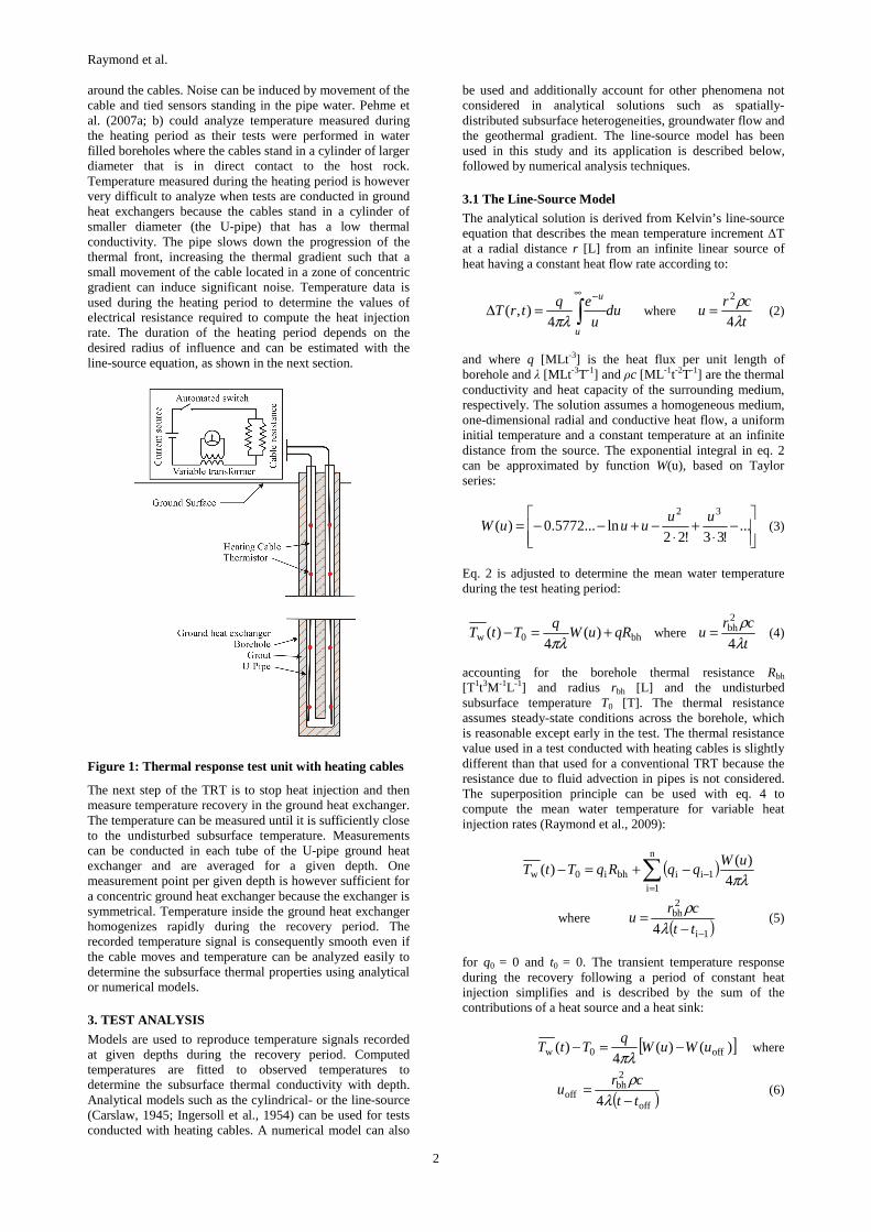
Heat transfer associated to a thermal response test using heating cables is mostly conductive. Any numerical model that can simulate heat conduction can potentially be used to reproduce the temperature measured during the TRT. A model that simulates advective heat transfer can additionally account for the effect of groundwater flow. The finite element/finte difference model HydroGeoSphere (Therrien et al., 2009) that can simulate heat transfer by conduction and advection (Graf and Therrien, 2007) was used for this study. A two-dimensional mesh (Fig. 2a) centered on the borehole and properly refined to discretize water, pipe, material filling the borehole and the subsurface is used to reproduce measurements recorded at a determined depth. Two-dimensional layers of the mesh are then stacked (Fig.2b) to simulate the TRT in three dimensions and simultaneously reproduce measurements recorded at all depths. Our simulations were conducted with a finite element representation using triangular elements in 2D and a node centered finite difference representation with triangular prism cells in 3D. The width of the triangular elements varied from 2 m near lateral boundaries to 0.002m at the borehole center. Layers stacked to build the 3D model were horizontally spaced by 1m. The numerical model HydroGeoSphere, having flexibility with grid refinement, helped to prepare meshes used for simulations.

Groundwater flow, if taken in account, is simulated in steady-state conditions while transient heat transfer simulations are performed. Full upstream weighting of velocities was chosen to resolve advective heat transfer equations such that the nodal temperature used in calculations is that of the upstream node. Using upstream weighting does not significantly changes temperature compared to central weighting but ensures that energy is conserved. The implicit Euler method was also selected, which implies building and solving a matrix at each timestep to resolve heat transfer. Computation time varied from 9 to 118 seconds using a desktop computer equipped with a 3.16GHZ dual core processor and 4GIG of RAM. The simulation time was optimized using adaptable timesteps that are constrained by a maximum change in temperature of 1 °C at all nodes and a maximum timestep of 1 hour.

Figure 2: a) Two- and b) three-dimensional mesh examples for analysis with numerical models

Hydraulic heads and temperatures equal to those measured before starting the test are used for initial conditions. A geothermal gradient is specified when considering three-dimensional analysis. No fluid flow and constant head boundary conditions are assigned to lateral external faces to reproduce the site hydraulic gradient. A constant temperature boundary condition is assigned to lateral faces having a no flow boundary condition. Third-type heat transfer boundary condition is selected at lateral faces of constant head boundaries. Temperature is calculated at the nodes of the selected faces based on the model fluid flow solution and an external temperature that is specified when choosing third-type boundary condition. No heat flow boundary conditions are used at the top and the bottom faces of the mesh, which assumes that heat flow near these boundaries is dominantly radial. Lateral boundaries must be placed at a distance that is beyond the test radius of influence. A distance of 4m from the borehole center was used for our simulations. Internal heat generation is assigned to the elements representing the heating cables. The term is equivalent to the heat flux dissipated by the cables and is varied with time such that it is equal to zero during the test recovery period.

The evolution of selected nodal temperatures at locations corresponding to those of the temperature sensors is compared to the measurements to analyze the TRT. Thermal properties of both the subsurface and the borehole can be varied to evaluate their influence on the model results.

4. TEST PRECISION

Errors associated with measurements can affect the precision at which the subsurface thermal conductivity can be determined with the proposed models. To evaluate the precision of the TRT, the uncertainty associated with the measurements is therefore compared to the sensitivity of the model parameters. The impact of the location of the cables and the sensors on the precision of the test is discussed later in the section describing illustrative simulations of the TRT.

Raymond et al.

4

4.1 Measurement Uncertainties

Data provided by the manufacturers are used to evaluate the uncertainty of direct measurements. The data logger and the thermistors used in this study measured temperature with an accuracy of ±0.2 C and a resolution of 0.05°C. The uncertainty associated with a calculated parameter ωR, such as the heat injection rate per unit meter (eq. 1), which depends on the calculated electrical tension and resistance and the cable length, is calculated from (Holman, 1984):

2

1

2

M

2

M2

2

M1

R

n

21

...⎥⎥⎥⎥⎥⎥

⎦

⎤

⎢⎢⎢⎢⎢⎢

⎣

⎡

⎟⎟⎠

⎞⎜⎜⎝

⎛∂∂++

⎟⎟⎠

⎞⎜⎜⎝

⎛∂∂+⎟⎟

⎠

⎞⎜⎜⎝

⎛∂∂

=

ω

ωωω

nM

R

M

R

M

R

(7)

where ωM1 to ωMn are the uncertainties of variables M1 to Mn with respect to function R. Using this relationship, the uncertainty of the electrical tension induced to the heating cable and the cable resistance varying with temperature were first determined during calibration shown in Appendix 1. The uncertainty associated with the calculation of the heat injection rate per unit meter, calculated with eq.7, is equal to ±3% for the worst cases. The influence of that uncertainty is accounted for in the sensitivity analysis described below.

4.2 Parameter Sensitivities

Factorial analyses (Box et al., 1978) are performed to evaluate the sensitivity of the subsurface thermal conductivity determined with the analytical and the numerical models during temperature recovery. The water temperature evolution for TRTs with a 50h heat injection followed by a 50h recovery in a ground heat exchanger made of a single U-pipe inserted in a 0.15 m diameter borehole is simulated. Parameters of the base case scenario presented in Table 1 are varied according to a determined uncertainty. Simulations are conducted with all possible combinations of parameters giving 2n temperature curves, where n is the number of parameters considered. The main effect of each parameter is evaluated from the change in temperature between the two scenarios where the varying parameter has a low and a high value. The parameter main effects are averaged for all comparison to determine the parameter effect on temperature as function of time.

The uncertainty specified for the heat injection rate in the factorial analyses is that of the measurements, which is ±3%. The uncertainty of the subsurface thermal conductivity is adjusted such that the effect of this unknown parameter is twice that of the heat injection rate for most duration of the simulations. This ensures that the effect of the subsurface thermal conductivity can be distinguished from that of the heat injection rate. It is also verified that the effect of the subsurface thermal conductivity remains above the temperature resolution for most duration of the simulations. This ensures that the effect of the subsurface thermal conductivity can be detected by temperature measurements. The resolution of temperature measurements is considered here instead of the accuracy because the models used calculate a temperature increase relative to the temperature at initial condition. The factorial analysis with uncertainties appropriately adjusted finally reveals the degree of precision associated with the subsurface thermal conductivity values determined during the TRT.

Table 1. Varying Parameters of the Base Case Scenario Used for the Factorial Analyses.

Parameter Value ± 3%

Unit Subsurface thermal conductivity 2.5 ± 6% Wm-1K-1 Grout thermal conductivity 1.4 ± 6% Wm-1K-1

Heat injection rate 30 ± 3% Wm-1

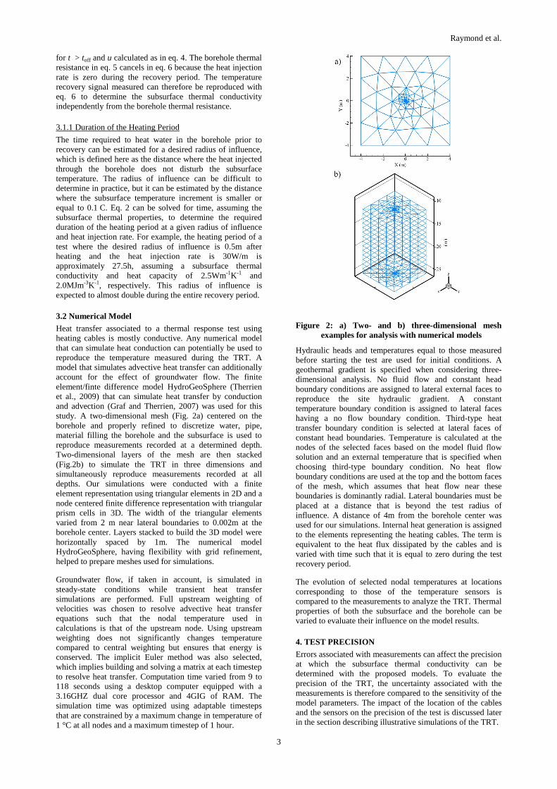
The line-source model used to calculate thermal recovery (eq. 6) is first subject to the factorial analysis. The subsurface heat capacity is not considered in the analysis because the effect of this parameter is negligible during the test recovery (Raymond et al., 2009). The factorial analysis results (Fig. 3a) show that the uncertainty at which the subsurface thermal conductivity can be determined is ±6%, which is twice that of the heat injection rate. This result was expected as the subtraction of the W functions in eq. 6 is near 1 during most of the recovery period which limits the temperature effect to the q/λ ratio.

The 2D numerical model described above is then subject to the factorial analysis. Groundwater flow is not simulated with the model at this stage. Only the thermal conductivity of the grout filling the borehole and the subsurface are considered with the heat injection rate for the factorial analysis. Other parameters such as the heat capacities of the

Figure 3: Results of the factorial analysis conducted to determine the parameter sensitivities of a) the line-source model and b) the numerical model. The effect on temperature for each parameter is plotted as function of time

Raymond et al.

5

different materials and the thermal conductivities of water and pipe are not accounted because they are either negligible or assumed constant. The factorial analysis (Fig. 3b) shows that the uncertainty at which the subsurface thermal conductivity can be determined is again twice that of the heat injection rate, which is ±6%. The same uncertainty was specified for the grout thermal conductivity but the effect of this parameter remains below that of the heat injection rate, which makes the estimation of the grout thermal conductivity difficult by this fact.

Factorial analyses were conducted with both the analytical and the numerical models with different combinations of parameters having good and poor heat transfer properties and gave similar results. It can be concluded that, in most situations, the relative precision at which the subsurface thermal conductivity can be determined from temperature recovery of a TRT is about twice that of the uncertainty associated to the heat injection rate.

5. ILUSTRATIVE EXAMPLES

A two-dimensional analysis of measurements recorded at a single depth is first reported below for a TRT performed on the campus of Université Laval in the Province of Québec, Canada. A three-dimensional analysis of a test with three measurements depths is then described for a second TRT performed at the Doyon Mine in the Abitibi Region of Québec.

5.1 Two-Dimensional Analysis

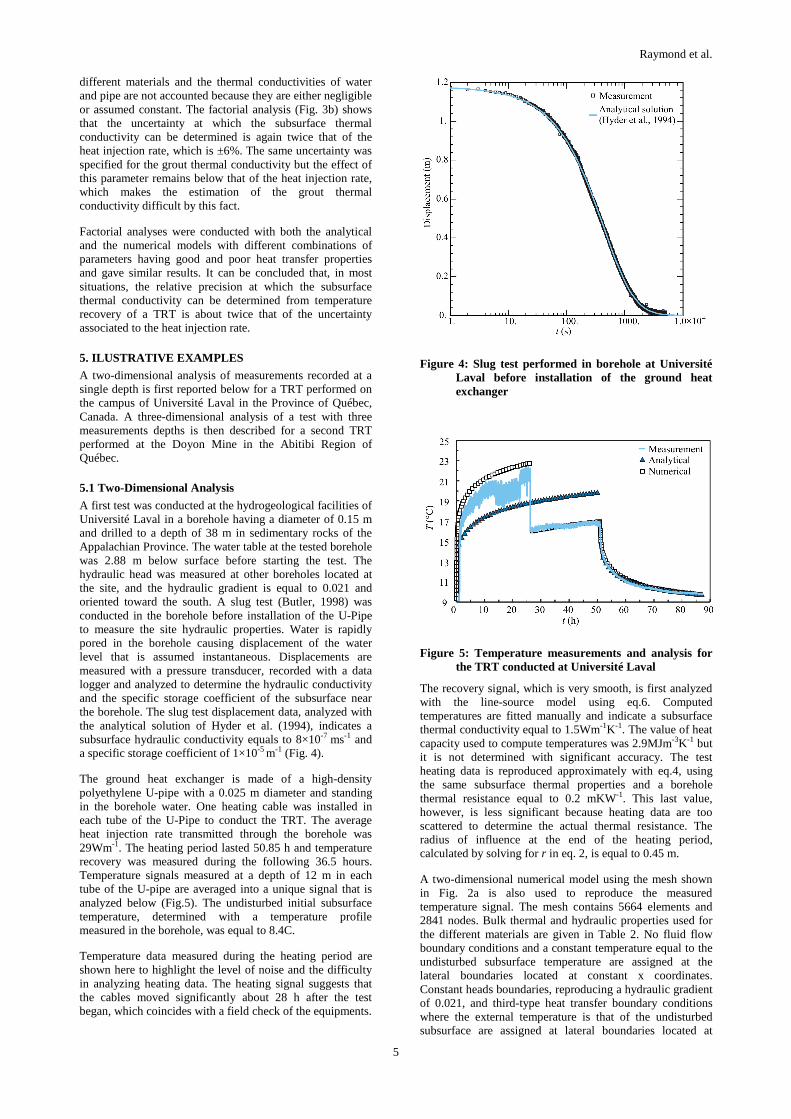
A first test was conducted at the hydrogeological facilities of Université Laval in a borehole having a diameter of 0.15 m and drilled to a depth of 38 m in sedimentary rocks of the Appalachian Province. The water table at the tested borehole was 2.88 m below surface before starting the test. The hydraulic head was measured at other boreholes located at the site, and the hydraulic gradient is equal to 0.021 and oriented toward the south. A slug test (Butler, 1998) was conducted in the borehole before installation of the U-Pipe to measure the site hydraulic properties. Water is rapidly pored in the borehole causing displacement of the water level that is assumed instantaneous. Displacements are measured with a pressure transducer, recorded with a data logger and analyzed to determine the hydraulic conductivity and the specific storage coefficient of the subsurface near the borehole. The slug test displacement data, analyzed with the analytical solution of Hyder et al. (1994), indicates a subsurface hydraulic conductivity equals to 8×10-7 ms-1 and a specific storage coefficient of 1×10-5 m-1 (Fig. 4).

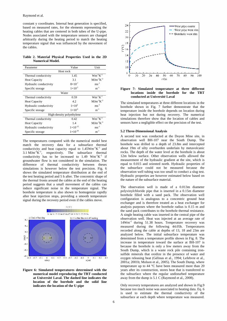
The ground heat exchanger is made of a high-density polyethylene U-pipe with a 0.025 m diameter and standing in the borehole water. One heating cable was installed in each tube of the U-Pipe to conduct the TRT. The average heat injection rate transmitted through the borehole was 29Wm-1. The heating period lasted 50.85 h and temperature recovery was measured during the following 36.5 hours. Temperature signals measured at a depth of 12 m in each tube of the U-pipe are averaged into a unique signal that is analyzed below (Fig.5). The undisturbed initial subsurface temperature, determined with a temperature profile measured in the borehole, was equal to 8.4C.

Temperature data measured during the heating period are shown here to highlight the level of noise and the difficulty in analyzing heating data. The heating signal suggests that the cables moved significantly about 28 h after the test began, which coincides with a field check of the equipments.

Figure 4: Slug test performed in borehole at Université Laval before installation of the ground heat exchanger

Figure 5: Temperature measurements and analysis for the TRT conducted at Université Laval

The recovery signal, which is very smooth, is first analyzed with the line-source model using eq.6. Computed temperatures are fitted manually and indicate a subsurface thermal conductivity equal to 1.5Wm-1K-1. The value of heat capacity used to compute temperatures was 2.9MJm-3K-1 but it is not determined with significant accuracy. The test heating data is reproduced approximately with eq.4, using the same subsurface thermal properties and a borehole thermal resistance equal to 0.2 mKW-1. This last value, however, is less significant because heating data are too scattered to determine the actual thermal resistance. The radius of influence at the end of the heating period, calculated by solving for r in eq. 2, is equal to 0.45 m.

A two-dimensional numerical model using the mesh shown in Fig. 2a is also used to reproduce the measured temperature signal. The mesh contains 5664 elements and 2841 nodes. Bulk thermal and hydraulic properties used for the different materials are given in Table 2. No fluid flow boundary conditions and a constant temperature equal to the undisturbed subsurface temperature are assigned at the lateral boundaries located at constant x coordinates. Constant heads boundaries, reproducing a hydraulic gradient of 0.021, and third-type heat transfer boundary conditions where the external temperature is that of the undisturbed subsurface are assigned at lateral boundaries located at

Raymond et al.

6

constant y coordinates. Internal heat generation is specified, based on measured rates, for the elements representing the heating cables that are centered in both tubes of the U-pipe. Nodes associated with the temperature sensors are changed arbitrarily during the heating period to match the heating temperature signal that was influenced by the movement of the cables.

Table 2. Material Physical Properties Used in the 2D Numerical Model.

Parameter Value Unit Host rock

Thermal conductivity 1.45 Wm-1K-1 Heat Capacity 3.1 MJm-3K-3

Hydraulic conductivity 8×10-7 ms-1

Specific storage 1×10-5 m-1

Water


Hydraulic conductivity 1×102 ms-1


High-density polyethylene




The temperatures computed with the numerical model best match the recovery data for a subsurface thermal conductivity and heat capacity equal to 1.45Wm-1K-1 and 3.1 MJm-3K-1, respectively. The subsurface thermal conductivity has to be increased to 1.49 Wm-1K-1 if groundwater flow is not considered in the simulation. The difference of thermal conductivity between theses simulations is however below the test precision. Fig. 6 shows the simulated temperature distribution at the end of the test heating period and 5 h after. The concentric shape of the thermal fronts around the cables at the end of the heating period suggests that a small movement of the cables can induce significant noise in the temperature signal. The borehole temperature is also shown to homogenize rapidly after heat injection stops, providing a smooth temperature signal during the recovery period even if the cables move.

Figure 6: Simulated temperatures determined with the numerical model reproducing the TRT conducted at Université Laval. The dashed line indicates the location of the borehole and the solid line indicates the location of the U-pipe

Figure 7: Simulated temperature at three different locations inside the borehole for the TRT conducted at Université Laval

The simulated temperatures at three different locations in the borehole shown in Fig. 7 further demonstrate that the temperature inside the borehole depends on location during heat injection but not during recovery. The numerical simulations therefore show that the location of cables and sensors have a negligible effect on the precision of the test.

5.2 Three-Dimensional Analysis

A second test was conducted at the Doyon Mine site, in observation well BH-107 near the South Dump. The borehole was drilled to a depth of 23.8m and intercepted about 19m of silty overburden underlain by metavolcanic rocks. The depth of the water level at the borehole is about 12m below surface. Other observation wells allowed the measurement of the hydraulic gradient at the site, which is equal to 0.015 and oriented north. Hydraulic properties of the subsurface could not be measured because the observation well tubing was too small to conduct a slug test. Hydraulic properties are however estimated below based on the nature of the subsurface material.

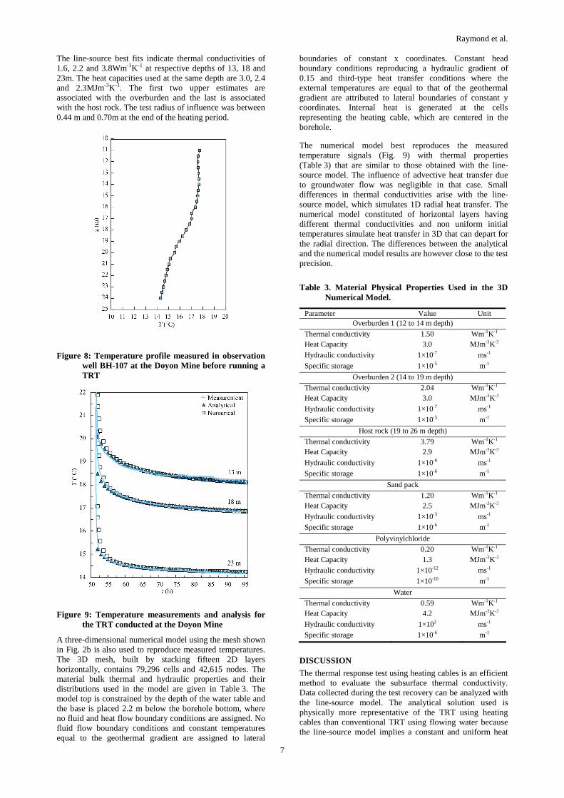
The observation well is made of a 0.013m diameter polyvinylchloride pipe that is inserted in a 0.15m diameter borehole filled with a sand pack. The observation well configuration is analogous to a concentric ground heat exchanger and is therefore treated as a heat exchanger for analysis purposes where the borehole radius is 0.15 m and the sand pack contributes to the borehole thermal resistance. A single heating cable was inserted in the central pipe of the observation well. Heat was injected at an average rate of 14Wm-1 during 51.38 hours. Temperature recovery was measured during the following 44.05h. Temperatures recorded along the cable at depths of 13, 18 and 23m are analyzed below. The initial subsurface temperature was determined from a temperature profile shown in Fig. 8. The increase in temperature toward the surface at BH-107 is because the borehole is only a few meters away from the South Dump, which is a waste rock pile containing iron-sulfide minerals that oxidize in the presence of water and oxygen releasing heat (Gélinas et al., 1994; Lefebvre et al., 2001a; 2001b; Molson et al., 2005). The South Dump, where temperature up to 44 °C have been measured more than 20 years after its construction, stores heat that is transferred to the subsurface where the regular undisturbed temperature away from the dump is 5.1 C (Raymond et al., 2008).

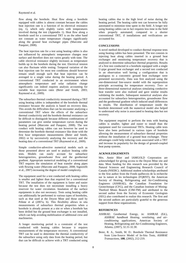
Only recovery temperatures are analyzed and shown in Fig.9 because too much noise was associated to heating data. Eq. 6 is used to estimate the thermal conductivity of the subsurface at each depth where temperature was measured.

Raymond et al.

7

The line-source best fits indicate thermal conductivities of 1.6, 2.2 and 3.8Wm-1K-1 at respective depths of 13, 18 and 23m. The heat capacities used at the same depth are 3.0, 2.4 and 2.3MJm-3K-1. The first two upper estimates are associated with the overburden and the last is associated with the host rock. The test radius of influence was between 0.44 m and 0.70m at the end of the heating period.

Figure 8: Temperature profile measured in observation well BH-107 at the Doyon Mine before running a TRT

Figure 9: Temperature measurements and analysis for the TRT conducted at the Doyon Mine

A three-dimensional numerical model using the mesh shown in Fig. 2b is also used to reproduce measured temperatures. The 3D mesh, built by stacking fifteen 2D layers horizontally, contains 79,296 cells and 42,615 nodes. The material bulk thermal and hydraulic properties and their distributions used in the model are given in Table 3. The model top is constrained by the depth of the water table and the base is placed 2.2 m below the borehole bottom, where no fluid and heat flow boundary conditions are assigned. No fluid flow boundary conditions and constant temperatures equal to the geothermal gradient are assigned to lateral

boundaries of constant x coordinates. Constant head boundary conditions reproducing a hydraulic gradient of 0.15 and third-type heat transfer conditions where the external temperatures are equal to that of the geothermal gradient are attributed to lateral boundaries of constant y coordinates. Internal heat is generated at the cells representing the heating cable, which are centered in the borehole.

The numerical model best reproduces the measured temperature signals (Fig. 9) with thermal properties (Table 3) that are similar to those obtained with the line-source model. The influence of advective heat transfer due to groundwater flow was negligible in that case. Small differences in thermal conductivities arise with the line-source model, which simulates 1D radial heat transfer. The numerical model constituted of horizontal layers having different thermal conductivities and non uniform initial temperatures simulate heat transfer in 3D that can depart for the radial direction. The differences between the analytical and the numerical model results are however close to the test precision.

Table 3. Material Physical Properties Used in the 3D Numerical Model.

Parameter Value Unit Overburden 1 (12 to 14 m depth)




Overburden 2 (14 to 19 m depth)




Host rock (19 to 26 m depth)




Sand pack




Polyvinylchloride




Water


Hydraulic conductivity 1×102 ms-1


DISCUSSION

The thermal response test using heating cables is an efficient method to evaluate the subsurface thermal conductivity. Data collected during the test recovery can be analyzed with the line-source model. The analytical solution used is physically more representative of the TRT using heating cables than conventional TRT using flowing water because the line-source model implies a constant and uniform heat

Raymond et al.

8

flow along the borehole. Heat flow along a borehole equipped with cables is almost constant because the cables heat injection rate is a function of its electrical resistance (eq. 1), which only slightly varies with temperatures involved during the test (Appendix 1). Heat flow along a borehole used for a conventional TRT is on the other hand not constant as water temperature changes significantly along the ground heat exchanger pipes (Marcotte and Pasquier, 2008).

The heat injection rate for a test using heating cables is also not influenced by atmospheric temperature changes near surface and therefore does not varies greatly with time. The cable electrical resistance slightly increases as temperature builds up in the borehole during the test. Electrical tension can also fluctuate while testing. Temporal variation of the heat injection rate for most test conditions should however remain small enough such that heat injection can be averaged to a single value during the heating period. A conventional TRT conducted in an environment where atmospheric temperature and solar radiation change significantly can indeed requires analysis accounting for variable heat injection rates (Beier and Smith, 2003; Raymond et al., 2009).

The subsurface thermal conductivity measured during a TRT using heating cables is independent of the borehole thermal resistance because the analysis is based on recovery data. This avoids the difficulties that can be encounter analyzing a conventional TRT where the effects of the subsurface thermal conductivity and the borehole thermal resistance can be difficult to distinguish because different combinations of parameters can give similar temperature curves during the heating period (Marcotte and Pasquier, 2008). The test conduct with heating cables can not however be used to determine the borehole thermal resistance like done with the first hour temperature measurements (Beier and Smith, 2002) or by successively analyzing the recovery and the heating data of a conventional TRT (Raymond et al., 2009).

Simple conductive-advective numerical models such as those presented above are used to analyze heating cable tests. Models can easily account for subsurface heterogeneities, groundwater flow and the geothermal gradient. Appropriate numerical modeling of a conventional TRT requires the simulation of heat transfer along pipes with flowing water (Marcotte and Pasquier, 2008; Signorelli et al., 2007) increasing the degree of model complexity.

The equipment used for a test conducted with heating cables is smaller and lighter than that required for a conventional TRT. The installation of the equipment is faster and easier because the test does not necessitate installing a heavy reservoir for water circulation. Insulation of the surface equipments is also not necessary. Tests using heating cable can additionally be performed in various types of boreholes, such as that used at the Doyon Mine and those used by Pehme et al (2007a; b). This flexibility allows in situ measurements of subsurface thermal properties when a borehole is already present at a site or when a borehole has been drilled but the ground heat exchanger is not installed, which can help avoiding mobilization of additional crew and machineries.

A longer monitoring period is a constraint of the test conducted with heating cables because it requires measurements of the temperature recovery. A conventional TRT can be used to determine the thermal conductivity of the subsurface using only data from the heating period, but that can be difficult to achieve with a TRT conducted using

heating cables due to the high level of noise during the heating period. The heating cable test can however be fully automated to minimize time spent in the field. A longer test using heating cables can in fact requires less time in the field when properly automated, compared to a shorter conventional TRT, if installations and verifications are accounted for.

CONCLUSIONS

A novel method developed to conduct thermal response tests using heating cables has been presented. The test consists in injecting heat along cables inserted in a ground heat exchanger and monitoring temperature recovery that is analyzed to determine subsurface thermal properties. Results of a first test conducted in a borehole equipped with a single U-pipe ground heat exchanger and a second test conducted in an observation well having a configuration that is analogous to a concentric ground heat exchanger were presented successively. Data was first analyzed using the one-dimensional line-source model with the superposition principle accounting for temperature recovery. Two- or three-dimensional numerical analyses simulating conductive heat transfer were also realized and gave similar results validating the models. Subsequent numerical analyses also accounted for subsurface heterogeneities, groundwater flow and the geothermal gradient which induced small differences in results. The distribution of temperature inside the borehole determined with the numerical model also helped to understand why noise is associated to heating data but not recovery.

The equipment required to perform the tests with heating cables is smaller, lighter and easier to install than the equipment used for conventional TRTs. Heating cable tests have also been performed in various types of borehole allowing the measurement of subsurface thermal properties without the installation of a ground heat exchanger. These advantages could help reducing costs associated with a TRT and increase its popularity for the design of ground-coupled heat pump systems.

ACKNOLEDGEMENTS

Mrs. Annie Blier and IAMGOLD Corporation are acknowledged for giving access to the Doyon Mine site and data. Most funding for this research was provided by the Natural Sciences and Engineering Research Council of Canada (NSERC). Additional student scholarships attributed to the first author from the Fonds québecois de la recherche sur la nature et les technologies (FQRNT), the American Society of Heating, Refrigerating and Air-Conditioning Engineers (ASHRAE), the Canadian Foundation for Geotechnique (CFG), and the Canadian Institute of Mining-Thetford Mines Branch (CIM-TM) and attributed to the second author from the Society of Economic Geologists (SEG) also contributed to realize this research. The first and the second authors are particularly grateful to the generous support from these organizations.

REFERENCES

ASHRAE: Geothermal Energy, in: ASHRAE (Ed.), ASHRAE handbook Heating, ventilating, and air-conditioning applications, American Society of Heating, Refrigerating and Air-Conditioning Engineers, Atlanta, (2007), 32.31-32.30.

Beier, R. A., Smith, M. D.: Borehole Thermal Resistance from Line-Source Model of In-Situ Tests, ASHRAE Transactions, 108, (2002), 212-219.

Raymond et al.

9

Beier, R. A., Smith, M. D.: Removing Variable Heat Rate Effects from Borehole Tests, ASHRAE Transactions, 109, (2003), 463-474.

Box, G.E.P., Hunter, W.G., Stuart Hunter, J.:Statistics for Experimenters. An Introduction to Design, Data Analysis and Model Building, John Wiely & Sons, New York (1978).

Butler, J.J.: The Design, Performance and Analysis of Slug Tests, CRC Press, Boca Raton (1998).

Carslaw, H. S.: Introduction to the mathematical theory of the conduction of heat in solids, Dover, New York, (1945).

Gehlin, S., Hellström, G.: Comparison of Four Models for Thermal Response Test Evaluation, ASHRAE Transactions, 109, (2003), 131-142.

Gélinas, P. J., Lefebvre, R., Choquette, M., Isabel, D., Locat, J., Guay, R.: Monitoring and modeling of acid mine drainage from waste rocks dumps, la Mine Doyon case study, Université Laval, Québec (1994).

Graf, T., Therrien, R.: Coupled thermohaline groundwater flow and single-species reactive solute transport in fractured porous media, Advances in Water Resources, 30, (2007), 742-771.

Holman, J.P.:1984. Experimental Methods for Engineers, McGraw-Hill, New York (1984).

Hurtig, E., Großwig, S., Jobmann, M., Kühn, K., Marschall, P.: Fibre-optic temperature measurements in shallow boreholes: experimental application for fluid logging, Geothermics, 23, (1994), 355-364.

Hurtig, E., Growig, S., Kühn, K.: Fibre optic temperature sensing: application for subsurface and ground temperature measurements, Tectonophysics, 257, (1996), 101-109.

Hyder, Z., Butler, J. J., McElwee, C. D., Liu, W. Z.: Slug Tests in Partially Penetrating Wells, Water Resources Research, 30, (1994), 2945-2957.

Ingersoll, L. R., Zobel, O. J., Ingersoll, A. C.: Heat conduction, with engineering, geological, and other applications, McGraw-Hill, New York, (1954).

Lefebvre, R., Hockley, D., Smolensky, J., Gélinas, P. J.: Multiphase transfer processes in waste rock piles producing acid mine drainage 1: Conceptual model and system characterization, Journal of Contaminant Hydrology, 52, (2001a), 137-164.

Lefebvre, R., Hockley, D., Smolensky, J., Lamontagne, A.: Multiphase transfer processes in waste rock piles producing acid mine drainage 2. Applications of numerical simulation, Journal of Contaminant Hydrology, 52, (2001b), 165-186.

Marcotte, D., Pasquier, P.: On the estimation of thermal resistance in borehole thermal conductivity test, Renewable Energy, 33, (2008), 2407-2415.

Molson, J. W., Fala, O., Aubertin, M., Bussiere, B.: Numerical simulations of pyrite oxidation and acid mine drainage in unsaturated waste rock piles, Journal of Contaminant Hydrology, 78, (2005), 343-371.

Pehme, P. E., Greenhouse, J. P., Parker, B. L.: The active line source (ALS) technique, a method to improve detection of hydraulically active fractures and estimate rock thermal conductivity, Proceedings, 60th Canadian Geotechnical Conference & 8th Joint CGS/IAH-CNC Groundwater Conference, Ottawa (2007a).

Pehme, P. E., Greenhouse, J. P., Parker, B. L.: The Active Line Source Temperature Logging Technique and Its Application in Fractured Rock Hydrogeology, Journal of Environmental and Engineering Geophysics, 12, (2007b), 307-322.

Raymond, J., Therrien, R., Gosselin, L., Lefebvre, R.: Thermal response test with variable heat injection rates, Proceedings, 62nd Canadian Geotechnical Conference & 10th Joint CGS/IAH-CNC Groundwater Conference, Halifax (2009).

Raymond, J., Therrien, R., Hassani, F.: Overview of geothermal energy resources in Québec (Canada) mining environments, Proceedings, 10th International Mine Water Congress, Karlovy Vary (2008).

Sanner, B., Hellstrom, G., Spitler, J. D., Gehlin, S. E. A.: Thermal response test - Current status and world-wide application, Proceedings, World Geothermal Energy Congress, Antalya (2005).

Signorelli, S., Bassetti, S., Pahud, D., Kohl, T.: Numerical evaluation of thermal response tests, Geothermics, 36, (2007), 141-166.

Therrien, R., McLaren, R. G., Sudicky, E. A., Panday, S. M.: HydroGeoSphere. A three-dimensional numerical model describing fully-integrated subsurface and surface flow and solute transport., Université Laval, Québec, University of Waterloo, Ontario (2009).

Raymond et al.

10

APPENDIX 1 – EQUIPEMENT CALIBRATION

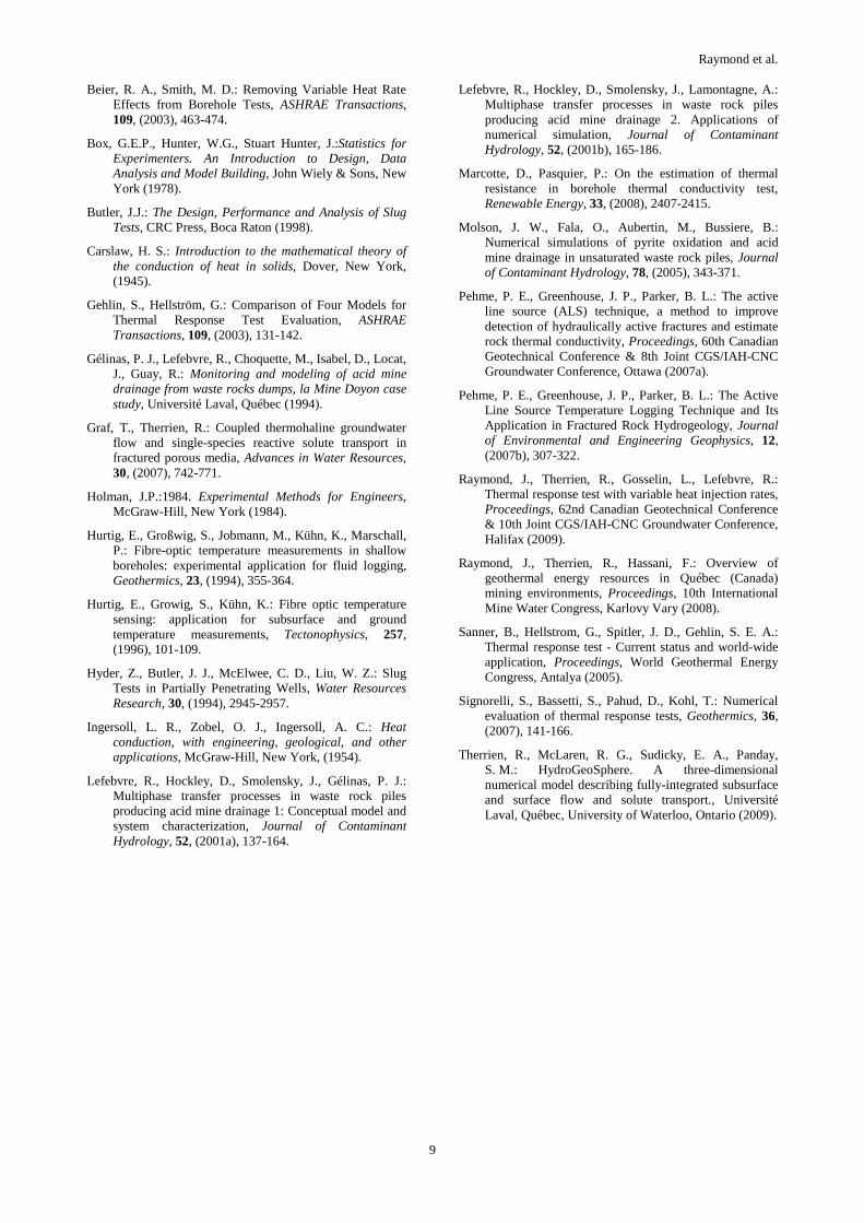
Conducting a thermal response test with heating cables requires equipment calibration. The heating cable electrical resistance was calibrated against temperature. Cables where put in a circulating bath where the water is heated using the cables and the water temperature is measured as function of the electrical resistance (Fig. 10). A linear fit to our measurements gave the following equation which is used to calculate the cable resistance:

4.3603.0 += TRe (8)

The uncertainty associated to the electrical resistance calculated using eq.8 is determined with eq. 7 and mostly depends on the uncertainty of the Ohmmeter used for calibration because the slope of the linear fit is small. Our equipment yielded a maximum uncertainty of ±0.5Ω for the electrical resistance calculation.

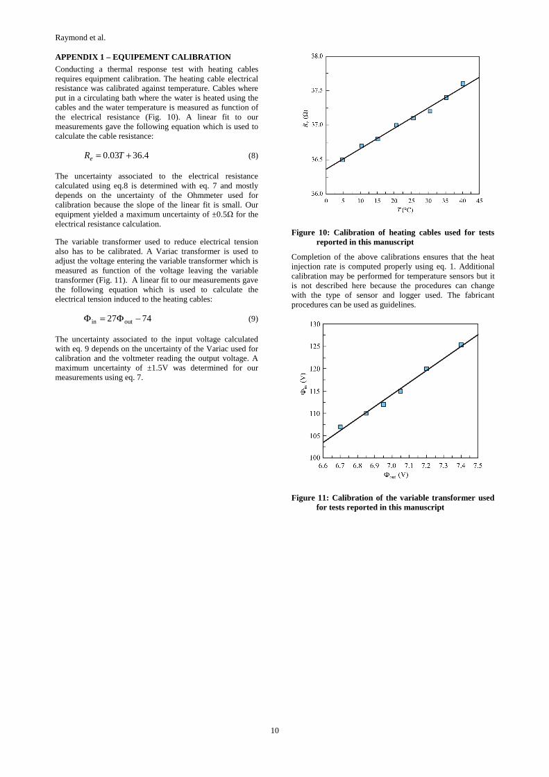
The variable transformer used to reduce electrical tension also has to be calibrated. A Variac transformer is used to adjust the voltage entering the variable transformer which is measured as function of the voltage leaving the variable transformer (Fig. 11). A linear fit to our measurements gave the following equation which is used to calculate the electrical tension induced to the heating cables:

7427 outin −Φ=Φ (9)

The uncertainty associated to the input voltage calculated with eq. 9 depends on the uncertainty of the Variac used for calibration and the voltmeter reading the output voltage. A maximum uncertainty of ±1.5V was determined for our measurements using eq. 7.

Figure 10: Calibration of heating cables used for tests reported in this manuscript

Completion of the above calibrations ensures that the heat injection rate is computed properly using eq. 1. Additional calibration may be performed for temperature sensors but it is not described here because the procedures can change with the type of sensor and logger used. The fabricant procedures can be used as guidelines.

Figure 11: Calibration of the variable transformer used for tests reported in this manuscript