7031 energy savings measurement guide - ceati ... · energy savings measurement guide. following...

ENERGY SAVINGS MEASUREMENT

GUIDE

Following the International Performance Measurement

and Verification Protocol

DISCLAIMER: Neither CEATI International, the authors, nor any of the organizations providing funding support for this work (including any persons acting on the behalf of the aforementioned) assume any liability or responsibility for any damages arising or resulting from the use of any information, equipment, product, method or any other process whatsoever disclosed or contained in this guide. The use of certified practitioners for the application of the information contained herein is strongly recommended. This guide was prepared by Environmental Interface Limited for the CEATI International Customer Energy Solutions Interest Group (CESIG) with the sponsorship of the following utility consortium participants:

© 2008 CEATI International. All rights reserved.

Appreciation to Ontario Hydro, Ontario Power Generation and others who have contributed material that has been used in preparing this guide.

TABLE OF CONTENTS

Section Page

1 Introduction 5 1.1 What Is Energy Savings Measurement? 5 1.2 Why Measure Energy Savings? 6

2 Fundamental Principles 9 3 The Energy Savings Measurement Process 11 4 Basic Methods and Examples 13

4.1 Measurement Boundary 16 4.2 Option A – Retrofit Isolation: Key Parameter

Measurement 18 4.2.1 Best Application of Option A 27

4.3 Option B – Retrofit Isolation: All Parameter Measurement 28

4.3.1 Best Application of Option B 39 4.4 Option C – Whole Facility 40

4.4.1 Best Application of Option C 49 4.5 Option D – Calibrated Simulation 50

4.5.1 Best Application of Option D 54 4.6 Choosing an Option 55

5 Common Issues 59 5.1 Baselines 59

5.1.1 Baseline Data 59

5.1.2 Baseline Period Length 59 5.1.3 Baseline Adjustments 61

5.2 Measurement Equipment 62 5.3 Sampling 66 5.4 On-Off Test 67 5.5 Cost - Accuracy Tradeoffs 68 5.6 Applying Energy Prices 73

6 Definitions 77 7 Other Resources 83 Appendix A: Contents of a Full M&V Plan 87 Appendix B: Contents of a Full Energy Savings Report 93

1 Introduction

5

1 INTRODUCTION

This guide highlights basic considerations for determining1 the energy and demand savings arising from an energy efficiency project. Key parts of the guide are extracted with permission from the widely referenced International Performance Measurement and Verification Protocol (IPMVP - freely available at www.evo-world.org) to ensure consistency with common practice. Other resources are listed in Chapter 7.

This guide is not a complete specification for the design of a savings measurement process. The support of professionals in the field2 should be sought for the detailed design and operation of a savings measurement process.

1.1 What Is Energy Savings Measurement?

The process of measuring energy savings is widely known as ‘‘Measurement and Verification’’. M&V is the process of using measurement to reliably determine actual savings created within an individual facility by an energy management program.

Energy savings cannot be directly measured, since they represent the absence of energy use. Instead, savings are determined by comparing measured use before and after

1 Often called measurement 2 A certification program for professionals in this field is operated jointly by the Association of Energy Engineers and the Efficiency Valuation Organization. See www.evo-world.org (services), or www.aeecenter.com/certification.

http://www.evo-world.org/


http://www.aeecenter.org/

1 Introduction

6

implementation of a project, making appropriate adjustments for changes in conditions.

M&V activities consist of some or all of the following:

• meter installation calibration and maintenance, • data gathering and screening, • development of a computation method and acceptable

estimates, • computations with measured data, and • reporting, quality assurance, and third party

verification of reports.

When there is little doubt about the outcome of a project, or no need to prove results to another party, M&V may not be necessary. However, it is still wise to verify that the installed equipment is able to produce the expected savings.

Verification of the potential to achieve savings involves regular inspection and commissioning of equipment. However, such verification of the potential to generate savings is not a measurement of savings.

1.2 Why Measure Energy Savings?

Energy savings measurement techniques (M&V) can be used by facility owners or energy efficiency project investors for the following purposes:

• Increase Energy Savings. Accurate determination of energy savings gives facility owners and managers valuable feedback on their energy conservation measures (ECMs). This feedback helps them adjust

1 Introduction

7

ECM design or operations to improve savings, achieve greater persistence of savings over time, and lower variations in savings.

• Document Financial Transactions. For some projects, the energy efficiency savings are the basis for performance-based financial payments and/or a guarantee in a performance contract.

• Enhance Financing for Efficiency Projects. A good M&V plan increases the transparency and credibility of reports on the outcome of efficiency investments. This credibility can increase the confidence that investors and sponsors have in energy efficiency projects, enhancing their chances of being financed.

• Improve Engineering Design and Facility Operations and Maintenance. The preparation of a good M&V plan encourages comprehensive project design by including all M&V costs in the project’s economics. Good M&V also helps managers discover and reduce maintenance and operating problems, while providing feedback for future project designs.

• Manage Energy Budgets. Even where savings are not planned, M&V techniques are used to adjust for changing facility operating conditions in order to set proper budgets and account for budget variances.

1 Introduction

8

2 Fundamental Principles

9

2 FUNDAMENTAL PRINCIPLES

The fundamental principles of good M&V practice are described below, in alphabetical order.

ACCURATE -- M&V reports should be as accurate as the M&V budget will allow. M&V costs should normally be small relative to the monetary value of the savings being evaluated. M&V expenditures should also be consistent with the financial implications of over- or under-reporting of a project’s performance. Accuracy tradeoffs should be accompanied by increased conservativeness in any estimates and judgements.

COMPLETE -- The reporting of energy savings should consider all effects of a project. M&V activities should use measurements to quantify the significant effects, while estimating all others.

CONSERVATIVE -- Where judgements are made about uncertain quantities, M&V procedures should be designed to under-estimate savings.

CONSISTENT -- The reporting of a project’s energy effectiveness should be consistent between:

• different types of energy efficiency projects; • different energy management professionals for any

one project; • different periods of time for the same project; and • energy efficiency projects and new energy supply

projects.

2 Fundamental Principles

10

‘Consistent’ does not mean ‘identical,’ since it is recognized that any empirically derived report involves judgements which may not be made identically by all reporters.

RELEVANT -- The determination of savings should measure the performance parameters of concern, or least well known, while other less critical or predictable parameters may be estimated.

TRANSPARENT -- All M&V activities should be clearly and fully disclosed. Full disclosure should include presentation of all of the elements defined in Appendices A and B for the contents of an M&V plan and a savings report, respectively.

The balance of this document presents a flexible framework of basic procedures and four Options for achieving M&V processes which follow these fundamental principles. Where the framework is silent or inconsistent for any specific application, these M&V principles should be used for guidance.

3 The Energy Savings Measurement Process

11

3 THE ENERGY SAVINGS MEASUREMENT PROCESS

Savings measurement involves six steps within any energy management endeavour:

1. DEVELOP AN M&V PLAN. Advance planning ensures that all data needed for savings determination will be available after implementation of the ECM(s), within an acceptable budget. An M&V plan should be developed while the project itself is being developed and should be included as part of the overall project budget.

The recommended contents of a full M&V plan are listed in Appendix A. Each topic listed therein should be considered in the M&V design, and be reported upon in an M&V plan that is kept available for future reference.

This activity may require installation of special meters or other measurement devices to obtain baseline data. Any special meters added should be carefully selected, calibrated, installed and commissioned.

2. VERIFY ECM INSTALLATION. After the ECM is installed, inspect the installed equipment and revised operating procedures to ensure that they conform to the design intent of the ECM.

3. REPORTING PERIOD DATA GATHERING. Gather energy and operating data from the reporting period, as defined in the M&V plan.

3 The Energy Savings Measurement Process

12

4. COMPUTE SAVINGS. Compute savings in energy and monetary units in accordance with the M&V plan.

5. REPORT SAVINGS. Report savings in accordance with the M&V plan. The contents of a full Savings Report are listed in Appendix B.

6. REVIEW SAVINGS. Energy managers should review the savings reports with the facility’s operating staff. Such reviews may uncover useful information about how the facility uses energy, or where operating staff could benefit from more knowledge of the energy consumption characteristics of their facility.

4 Basic Methods and Examples

4 BASIC METHODS AND EXAMPLES

Energy or demand savings cannot be directly measured, since savings represent the absence of energy use or demand. Instead, savings are determined by comparing measured use or demand before and after implementation of a program, making suitable adjustments for changes in conditions.

A

13

Time

Ener

gy U

se

Reporting Period Measured Energy

djusted Baseline Energy

ECM Installation

Baseline Energy

Inreased Production

Sa v in g s, o r A v o id Ed En er g y U se

Reporting Period

Baseline Period

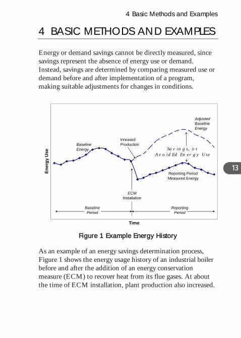
Figure 1 Example Energy History

As an example of an energy savings determination process, Figure 1 shows the energy usage history of an industrial boiler before and after the addition of an energy conservation measure (ECM) to recover heat from its flue gases. At about the time of ECM installation, plant production also increased.


To properly document the impact of the ECM, its energy effect must be separated from the energy effect of the increased production. The ‘‘baseline energy’’ use pattern before ECM installation was studied to determine the relationship between energy use and production. Following ECM installation, this baseline relationship was used to estimate how much energy the plant would have used each month if there had been no ECM (called the ‘‘adjusted baseline energy’’). The savings, or ‘avoided energy use’ is the difference between the adjusted baseline energy and the energy that was actually metered during the reporting period.

Without the adjustment for the change in production, the difference between baseline energy and reporting period energy would have been much lower, under-reporting the effect of the heat recovery.

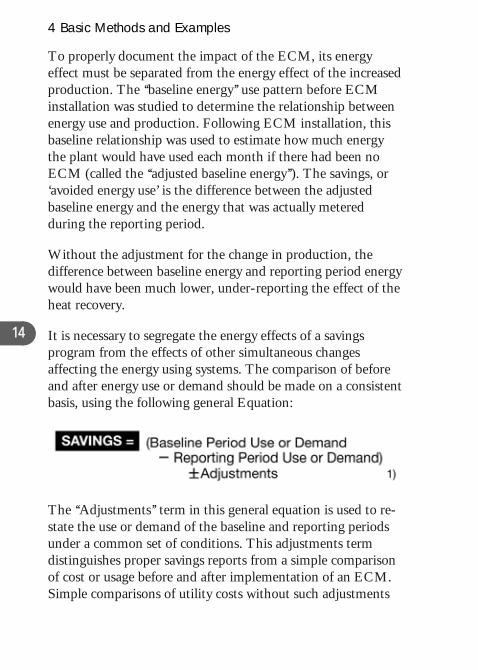
14 It is necessary to segregate the energy effects of a savings program from the effects of other simultaneous changes affecting the energy using systems. The comparison of before and after energy use or demand should be made on a consistent basis, using the following general Equation:

The ‘‘Adjustments’’ term in this general equation is used to re-state the use or demand of the baseline and reporting periods under a common set of conditions. This adjustments term distinguishes proper savings reports from a simple comparison of cost or usage before and after implementation of an ECM. Simple comparisons of utility costs without such adjustments


15

report only cost changes and fail to report the true performance of a project or facility. To properly report savings, adjustments must account for the differences in conditions between the baseline and reporting periods.

Savings are commonly computed in Equation 1) by adjusting baseline energy use to the conditions of the reporting period. Using this form of adjustment, savings can be thought of as ‘‘avoided energy (or cost).’’ This common form of expression of savings is the amount of energy (or dollars) not expended during the reporting period, as a result of the project.

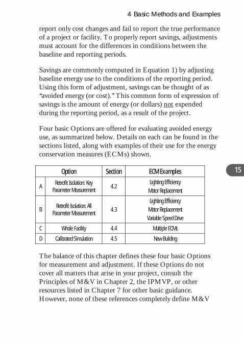
Four basic Options are offered for evaluating avoided energy use, as summarized below. Details on each can be found in the sections listed, along with examples of their use for the energy conservation measures (ECMs) shown.

Option Section ECM Examples

A Retrofit Isolation: Key Parameter Measurement

4.2 Lighting Efficiency

Motor Replacement

B Retrofit Isolation: All

Parameter Measurement 4.3 Lighting Efficiency

Motor Replacement Variable Speed Drive

C Whole Facility 4.4 Multiple ECMs

D Calibrated Simulation 4.5 New Building

The balance of this chapter defines these four basic Options for measurement and adjustment. If these Options do not cover all matters that arise in your project, consult the Principles of M&V in Chapter 2, the IPMVP, or other resources listed in Chapter 7 for other basic guidance. However, none of these references completely define M&V


16

practice for the wide range of possible situations. Professional judgment is warranted in application of the methods shown here or in the IPMVP.

4.1 Measurement Boundary

Savings may be determined for an entire facility or simply for a portion of it, depending upon the purposes of the reporting.

• If the purpose of reporting is to help manage only the equipment affected by the savings program, a measurement boundary should be drawn around that equipment. Then all significant energy requirements of the equipment within the boundary can be determined. This approach is used in the Retrofit Isolation Options of Chapters 4.2 and 4.3, below.

• If the purpose of reporting is to help manage total facility energy performance, the meters measuring the supply of energy to the total facility can be used to assess performance and savings. The measurement boundary in this case encompasses the whole facility. The Whole Facility Option C is described in Chapter 4.4, below.


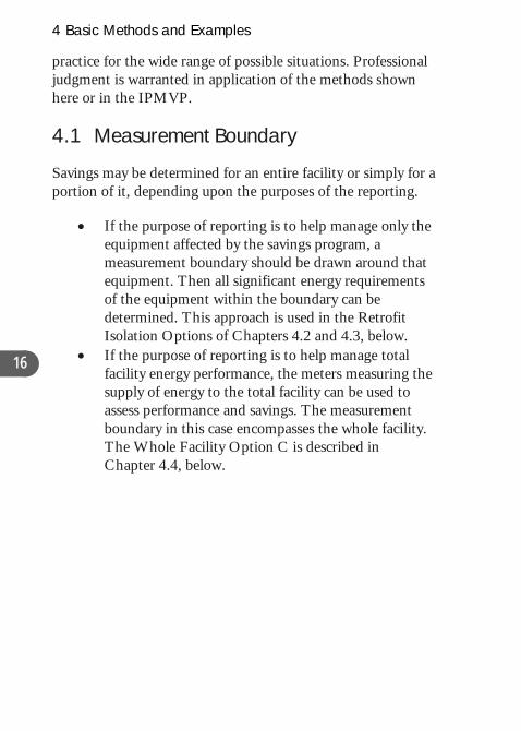
Figure 2 Measurement Boundary 17

The energy quantities in savings Equation 1) can be measured by one or more of the following techniques:

• Utility or fuel supplier invoices, or reading utility meters and making the same adjustments to the readings that the utility makes.

• Special meters isolating an ECM or portion of a facility from the rest of the facility. Measurements may be periodic for short intervals, or continuous throughout the baseline or reporting periods.

• Separate measurements of parameters used in computing energy use. For example, equipment operating parameters of electrical load and operating hours can be measured separately and multiplied together to compute the equipment’s energy use.


18

• Measurement of proven proxies for energy use. For example, if the energy use of a motor has been correlated to the output signal from the variable speed drive controlling the motor, the output signal could be a proven proxy for motor energy.

• Computer simulation that is calibrated to some actual performance data for the system or facility being modeled. One example of computer simulation is DOE-2 analysis for buildings (Option D only).

If an energy value is already known with adequate accuracy or when it is more costly to measure than justified by the circumstances, then measurement of energy may not be necessary or appropriate. In these cases, estimates may be made of some ECM parameters, but others must be measured (Option A only).

There are many ways to combine the choices of measurement boundary and measurement technique. IPMVP defines four basic combinations to suit a range of cost and accuracy requirements. The four Options are described in the rest of Chapter 4, with example applications. Chapter 5 discusses the common issues, such as the cost/accuracy tradeoffs, affecting all four Options.

4.2 Option A – Retrofit Isolation: Key Parameter Measurement

When savings measurement is focused on only the ECM, not the entire facility, ‘‘isolation’’ meters must be in place to measure the energy use of the systems affected by the ECM,


19

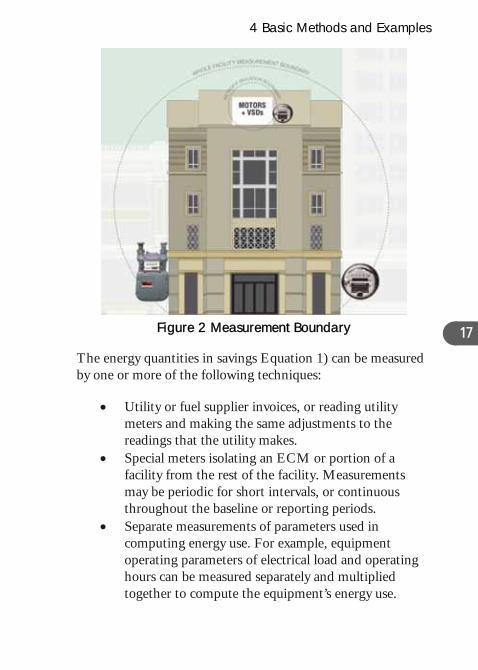
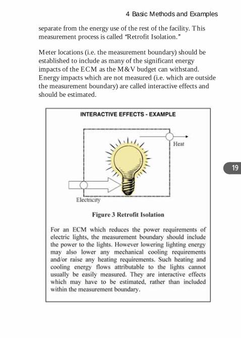
separate from the energy use of the rest of the facility. This measurement process is called ‘‘Retrofit Isolation.’’

Meter locations (i.e. the measurement boundary) should be established to include as many of the significant energy impacts of the ECM as the M&V budget can withstand. Energy impacts which are not measured (i.e. which are outside the measurement boundary) are called interactive effects and should be estimated.


Under Option A, savings are determined by field measurement of the key performance parameter(s) which define the energy use of the ECM’s affected system(s) and/or the success of the project.

The frequency of measurement ranges from short term to continuous, depending on the expected variations in the measured parameter, and the length of the reporting period.

Parameters not selected for field measurement are estimated. Estimates can be based on historical data, manufacturer’s specifications, or engineering judgment. Documentation of the source, or justification of the estimated parameter, is required. The plausible savings error arising from estimation rather than measurement is evaluated.

Savings are calculated by engineering calculation of baseline and reporting period energy from: 20

• Short term or continuous measurements of key operating parameter(s); and

• estimated values.

This is a simplification of Equation 1), above, suited to the common situation of no changes occurring in operating conditions between the baseline and reporting periods. If there are changes, measured parameters must be adjusted to the same conditions. However the estimated value can be for any set of conditions chosen.


EXAMPLE 1 -- Lighting Efficiency -- Option A

An office building’s lighting retrofit project replaced all lamps and ballasts with more efficient ones. The wattages of the new lamp/ballast combinations were well known. However wattage of the old ones varied considerably due to the variety of replacements that had taken place since the lighting system was originally installed. It was therefore decided that lighting power was the key parameter that should be measured under IPMVP Option A

A calibrated portable true rms wattmeter was used to measure the power to the five lighting breaker panels December 2, 2007, before retrofit. The same measurement was made on July 23, 2008, three weeks after retrofit so that lamps had time to stabilize in their power draw. Measurements were made with all lighting circuit breakers in their on position and any local switches in the on position. This measurement boundary at the panels does not include the interactive effects of the lights on the heating and cooling systems. Therefore interactive effects were analyzed as follows:

21

• In 7 winter months, extra boiler heat would be needed to replace lost heat from lighting in the building’s perimeter zones. Perimeter zones were 50% of the floor space (and 50% of the lights). Perimeter zone heat was supplied by a gas fired boiler with an unmeasured efficiency rating of 84%. It was estimated that net heat delivered to the perimeter space by the boiler would be only 80% of the energy entering the boiler. Therefore, it was estimated that every kW of lighting load reduction requires 0.63 equivalent kW of


22

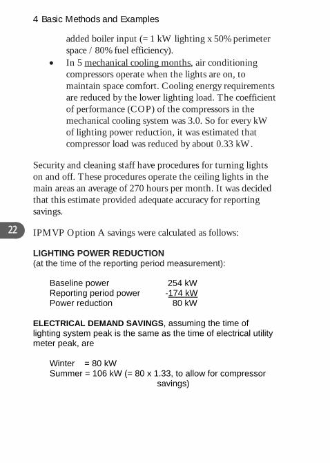
added boiler input (= 1 kW lighting x 50% perimeter space / 80% fuel efficiency).

• In 5 mechanical cooling months, air conditioning compressors operate when the lights are on, to maintain space comfort. Cooling energy requirements are reduced by the lower lighting load. The coefficient of performance (COP) of the compressors in the mechanical cooling system was 3.0. So for every kW of lighting power reduction, it was estimated that compressor load was reduced by about 0.33 kW.

Security and cleaning staff have procedures for turning lights on and off. These procedures operate the ceiling lights in the main areas an average of 270 hours per month. It was decided that this estimate provided adequate accuracy for reporting savings.

IPMVP Option A savings were calculated as follows:

LIGHTING POWER REDUCTION (at the time of the reporting period measurement):

Baseline power 254 kW Reporting period power -174 kW Power reduction 80 kW

ELECTRICAL DEMAND SAVINGS, assuming the time of lighting system peak is the same as the time of electrical utility meter peak, are

Winter = 80 kW Summer = 106 kW (= 80 x 1.33, to allow for compressor

savings)


23

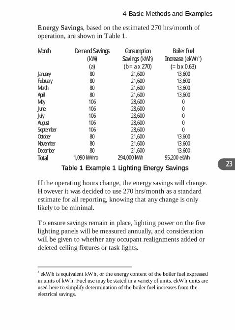
Energy Savings, based on the estimated 270 hrs/month of operation, are shown in Table 1.

Month Demand Savings (kW) (a)

Consumption Savings (kWh) (b = a x 270)

Boiler Fuel Increase (ekWh3)

(= b x 0.63) January 80 21,600 13,600 February 80 21,600 13,600 March 80 21,600 13,600 April 80 21,600 13,600 May 106 28,600 0 June 106 28,600 0 July 106 28,600 0 August 106 28,600 0 September 106 28,600 0 October 80 21,600 13,600 November 80 21,600 13,600 December 80 21,600 13,600 Total 1,090 kW-mo 294,000 kWh 95,200 ekWh

Table 1 Example 1 Lighting Energy Savings

If the operating hours change, the energy savings will change. However it was decided to use 270 hrs/month as a standard estimate for all reporting, knowing that any change is only likely to be minimal.

To ensure savings remain in place, lighting power on the five lighting panels will be measured annually, and consideration will be given to whether any occupant realignments added or deleted ceiling fixtures or task lights.

3 ekWh is equivalent kWh, or the energy content of the boiler fuel expressed in units of kWh. Fuel use may be stated in a variety of units. ekWh units are used here to simplify determination of the boiler fuel increases from the electrical savings.


24

Annual savings could then be reported as adhering to IPMVP Vol I, 2007, Option A if the following statement is made: ‘‘Annual avoided electricity use, based on the measurement taken on July 23, 2008 and estimated annual operating periods, are determined to be 294,000 kWh and 1,090 kW-months. On the same basis it is estimated that boiler fuel requirements increased by 95,200 equivalent kWh.’’

Note: If there had been a high degree of confidence in the baseline power, (i.e. all fixtures had identical equipment), it may be decided to use manufacturer ratings for power draw of the baseline and retrofit equipment. Such approach is certainly the least expensive form of savings reporting. However it does not involve a field measurement of the key parameter defining the ECM. Savings reports without field measurement of the key parameter do not adhere to IPMVP, since it is a performance ‘measurement’ protocol. An IPMVP Option A savings report must measure in the field either the load change or the operating hours.

See also Chapter 5.6, Example 9, where the dollar value of Example 1 electrical savings is computed.

EXAMPLE 2 -- Motor Replacement -- Option A

An industrial plant replaced all motors above 10hp with new high efficiency types. 40 motors were changed, ranging in size from 15 to 100 hp. In some cases the new motors were smaller to better suit the current loads. The motors drove fans, pumps and conveyors. They were all operating at constant speeds and constant loads.

Group A operated when the plant was in operation, normally 5,376 hours per year. Group B served building ventilation


25

systems which operate regardless of plant operations, i.e. 8,760 hrs/year. Group C serves heating systems which usually only operate about 3,100 hrs/year.

The measurement boundary was established as the motors themselves with no interactive effects. Though the more efficient motors drove their loads slightly faster, there was no energy effect other than on the motor power draw itself. The inventory of motors, driven equipment and their speeds were recorded before retrofit.

The operating hours of Groups A and B were highly predictable, as long as the plant continued at two shifts per day for 48 weeks per year. Group C operating hours depend on heating system operating periods which vary somewhat from year to year. The possible 2-300 hours of variation were not considered significant to the overall savings results. Therefore the above operating hours were set as the estimate that would be used for establishing Option A savings.

Baseline data was gathered with a portable true rms wattmeter measuring and logging the electrical draw on each motor over an eight hour shift. Each motor’s record was examined to ensure that its load was essentially constant.

After retrofit the same readings were taken during the month of March 2007, and the loads were again assessed as being constant. Since plant electrical load patterns were known to normally be steady during production, it can safely be assumed that production and ventilation motors operate during the time of establishment of peak demand on the electric utility meter. However the heating system motors will only affect peak


26

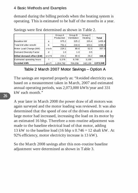
Group A Group B Group CProduction Ventilation Heating Total

Baseline kW a 975.2 325.2 155.4 1455.8

Total kW after retrofi t b 751.1 244.6 103.1 1098.8Motor Load Change (kW) c=a-b 224.1 80.6 52.3 357.0Demand Diversity Factor d 1.0 1.0 0.5

Billed demand effect (kW) e=c*d 224.1 80.6 26.2 330.9Estimated operating hours f 5,376 8,760 3,100 Avoided kWh g=c*f 1,204,762 706,056 162,130 2,072,948

demand during the billing periods when the heating system is operating. This is estimated to be half of the months in a year.

Savings were first determined as shown in Table 2.

Table 2 March 2007 Motor Savings – Option A

The savings are reported properly as: ‘‘Avoided electricity use, based on a measurement taken in March, 2007 and estimated annual operating periods, was 2,073,000 kWh/year and 331 kW each month.’’

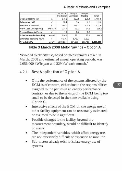
A year later in March 2008 the power draw of all motors was again surveyed and the motor loading was reviewed. It was also determined that the speed of one of the driven elements on a large motor had increased, increasing the load on its motor by an estimated 16 bhp. Therefore a non-routine adjustment was made to the baseline electrical load of that motor, adding 13 kW to the baseline load (16 bhp x 0.746 = 12 shaft kW. At 92% efficiency, motor electricity increase is 13 kW).

So the March 2008 savings after this non-routine baseline adjustment were determined as shown in Table 3.


27

Group A Group B Group CProduction Ventilation Heating Total

Original Baseline kW a 975.2 325.2 155.4 1,455.8 Adjustment kW a' 13.0 0.0 0.0 13.0 Total kW after retrofit b 764.2 247.1 101.3 1,112.6 Motor Load Change (kW) c=a+a'-b 224.0 78.1 54.1 356.2

Demand Diversity Factor d 1.0 1.0 0.5Billed demand effect (kW) e=c*d 224.0 78.1 27.1 329.2Estimated operating hours f 5,376 8,760 3,100 Avoided kWh g=c*f 1,204,224 684,156 167,710 2,056,090

Table 3 March 2008 Motor Savings – Option A

‘‘Avoided electricity use, based on measurements taken in March, 2008 and estimated annual operating periods, was 2,056,000 kWh/year and 329 kW each month.’’

4.2.1 Best Application of Option A

• Only the performance of the systems affected by the ECM is of concern, either due to the responsibilities assigned to the parties in an energy performance contract, or due to the savings of the ECM being too small to be detected in the time available using Option C.

• Interactive effects of the ECM on the energy use of other facility equipment can be reasonably estimated, or assumed to be insignificant.

• Possible changes to the facility, beyond the measurement boundary, would be difficult to identify or assess.

• The independent variables, which affect energy use, are not excessively difficult or expensive to monitor.

• Sub-meters already exist to isolate energy use of systems.


• Meters added at the measurement boundary can be used for other purposes such as operational feedback or tenant billing.

• Measurement of parameters is less costly than Option D simulations or Option C non-routine adjustments.

• Long term testing is not warranted. • There is no need to directly reconcile savings reports

with changes in payments to energy suppliers. • Estimation of key parameters may avoid possibly

difficult non-routine adjustments when future changes happen within the measurement boundary.

• The uncertainty created by estimations is acceptable. • The continued effectiveness of the ECM can be

assessed by simple routine inspection. • Estimation of some parameters is less costly than

measurement of them in Option B or simulation in Option D.

28

• A key parameter used in computing savings is well known. Key parameters are parameters used to judge a project’s or contractor’s performance.

4.3 Option B – Retrofit Isolation: All Parameter Measurement

Option B is similar to Option A in that it draws a measurement boundary around the ECM, smaller than the entire facility. However it differs from Option A in requiring either measurement of all ECM parameters used to compute energy, or measurement of energy use itself.


29

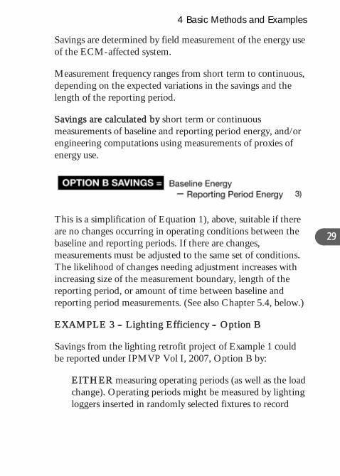
Savings are determined by field measurement of the energy use of the ECM-affected system.

Measurement frequency ranges from short term to continuous, depending on the expected variations in the savings and the length of the reporting period.

Savings are calculated by short term or continuous measurements of baseline and reporting period energy, and/or engineering computations using measurements of proxies of energy use.

This is a simplification of Equation 1), above, suitable if there are no changes occurring in operating conditions between the baseline and reporting periods. If there are changes, measurements must be adjusted to the same set of conditions. The likelihood of changes needing adjustment increases with increasing size of the measurement boundary, length of the reporting period, or amount of time between baseline and reporting period measurements. (See also Chapter 5.4, below.)

EXAMPLE 3 -- Lighting Efficiency -- Option B

Savings from the lighting retrofit project of Example 1 could be reported under IPMVP Vol I, 2007, Option B by:

EITHER measuring operating periods (as well as the load change). Operating periods might be measured by lighting loggers inserted in randomly selected fixtures to record


lighting operating periods. The guidance of Chapter 5.3 may assist in sampling.

Figure 4 Lighting Logger The lighting system energy use is then computed by multiplying the measured load change by the measured operating periods of the reporting period;

30

OR measuring lighting panel electricity consumption (kWh) with electrical energy meter(s).

Such full measurements would be made for both the baseline and reporting periods.

For this Example 3, a kWh meter was installed on each lighting panel for a week in the baseline period (see Figure 5).


0

50

100

150

200

250

300

1 9 17 25 33 41 49 57 65 73 81 89 97 105

113

121

129

137

145

153

161

Hour

kWh

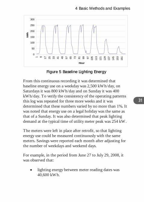
Figure 5 Baseline Lighting Energy

From this continuous recording it was determined that baseline energy use on a weekday was 2,500 kWh/day, on Saturdays it was 800 kWh/day and on Sunday it was 400 kWh/day. To verify the consistency of the operating patterns this log was repeated for three more weeks and it was determined that these numbers varied by no more than 1%. It was noted that energy use on a legal holiday was the same as that of a Sunday. It was also determined that peak lighting demand at the typical time of utility meter peak was 254 kW.

31

The meters were left in place after retrofit, so that lighting energy use could be measured continuously with the same meters. Savings were reported each month after adjusting for the number of weekdays and weekend days.

For example, in the period from June 27 to July 29, 2008, it was observed that:

• lighting energy between meter reading dates was 40,600 kWh.


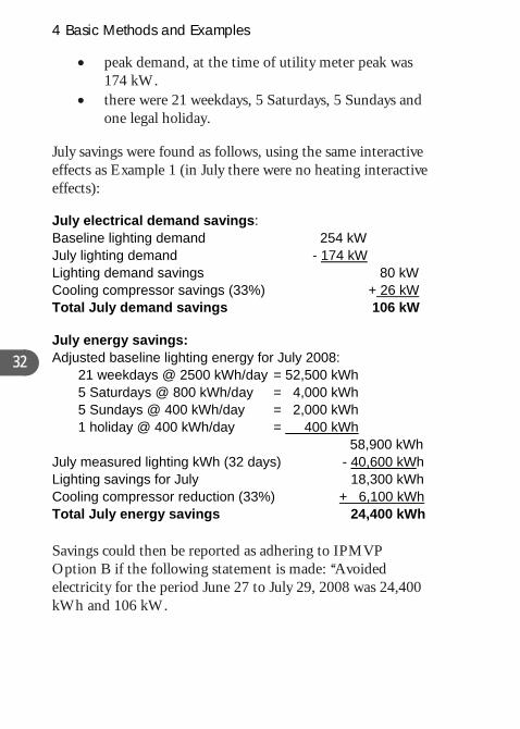
• peak demand, at the time of utility meter peak was 174 kW.

• there were 21 weekdays, 5 Saturdays, 5 Sundays and one legal holiday.

July savings were found as follows, using the same interactive effects as Example 1 (in July there were no heating interactive effects):

July electrical demand savings: Baseline lighting demand 254 kW July lighting demand - 174 kW Lighting demand savings 80 kW Cooling compressor savings (33%) + 26 kW Total July demand savings 106 kW

July energy savings: Adjusted baseline lighting energy for July 2008: 32

21 weekdays @ 2500 kWh/day = 52,500 kWh 5 Saturdays @ 800 kWh/day = 4,000 kWh 5 Sundays @ 400 kWh/day = 2,000 kWh 1 holiday @ 400 kWh/day = 400 kWh

58,900 kWh July measured lighting kWh (32 days) - 40,600 kWh Lighting savings for July 18,300 kWh Cooling compressor reduction (33%) + 6,100 kWh Total July energy savings 24,400 kWh

Savings could then be reported as adhering to IPMVP Option B if the following statement is made: ‘‘Avoided electricity for the period June 27 to July 29, 2008 was 24,400 kWh and 106 kW.


33

This process would continue as long as lighting energy was a concern. The process would include recording of the number of each type of day in each metering period, and reading the meters once a month. Annual review would also be made of the number of fixtures in place, the occupancy periods and cooling/heating plant efficiencies so that adjustments could be made for any such non-routine changes to baseline conditions.

Note:

1. This Option B measurement approach could also assess the impact of an ECM installing lighting controls, such as occupancy sensors.

2. Option A above for this example measured a savings of 28,600 kWh and a demand reduction of 106 kW so the addition of the lighting logger increased the accuracy of the measurements.

EXAMPLE 4 -- Motor Replacement -- Option B

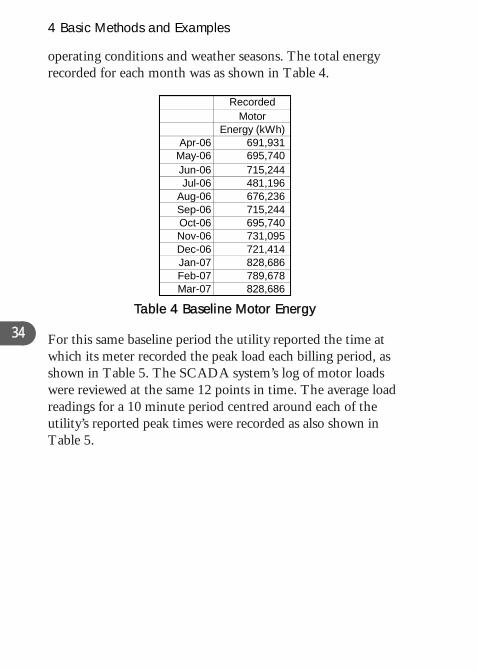
The savings determined in Example 2 (Option A) could be presented with more certainty, but probably at higher cost, by using Option B. In Option B, all parameters of the reported savings must be measured, not just the key parameter of motor electrical load. This requires measurement, for the baseline and reporting periods, of motor kWh consumption, and motor demand at the time of utility meter peak.

To measure electrical load, motor current and voltage transducers and kWh loggers were added to the monitoring equipment at each motor before retrofit. Data was gathered by the plant SCADA system every 5 minutes for each motor for a one year period before retrofit. This period covered all plant


34

RecordedMotor

Energy (kWh)Apr-06 691,931

May-06 695,740 Jun-06 715,244 Jul-06 481,196

Aug-06 676,236 Sep-06 715,244 Oct-06 695,740 Nov-06 731,095 Dec-06 721,414 Jan-07 828,686 Feb-07 789,678 Mar-07 828,686

operating conditions and weather seasons. The total energy recorded for each month was as shown in Table 4.

Table 4 Baseline Motor Energy

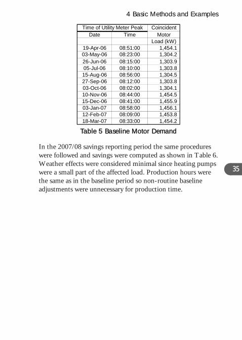
For this same baseline period the utility reported the time at which its meter recorded the peak load each billing period, as shown in Table 5. The SCADA system’s log of motor loads were reviewed at the same 12 points in time. The average load readings for a 10 minute period centred around each of the utility’s reported peak times were recorded as also shown in Table 5.


35

Time of Utility Meter Peak CoincidentDate Time Motor

Load (kW)19-Apr-06 08:51:00 1,454.1 03-May-06 08:23:00 1,304.2 26-Jun-06 08:15:00 1,303.9 05-Jul-06 08:10:00 1,303.8 15-Aug-06 08:56:00 1,304.5 27-Sep-06 08:12:00 1,303.8 03-Oct-06 08:02:00 1,304.1 10-Nov-06 08:44:00 1,454.5 15-Dec-06 08:41:00 1,455.9 03-Jan-07 08:58:00 1,456.1 12-Feb-07 08:09:00 1,453.8 18-Mar-07 08:33:00 1,454.2

Table 5 Baseline Motor Demand

In the 2007/08 savings reporting period the same procedures were followed and savings were computed as shown in Table 6. Weather effects were considered minimal since heating pumps were a small part of the affected load. Production hours were the same as in the baseline period so non-routine baseline adjustments were unnecessary for production time.


36

Baseline 2007/08 Measurements Savings

Energy Demand Energy Demand Energy Demand(kWh) Load (kW) (kWh) Load (kW) (kWh) Load (kW)

Apr-07 691,931 1,454.1 510,904 1,073.7 181,027 380.4 May-07 695,740 1,304.2 510,758 957.4 184,982 346.8

Jun-07 715,244 1,303.9 524,410 956.0 190,834 347.9

Jul-07 481,196 1,303.8 360,577 977.0 120,619 326.8 Aug-07 676,236 1,304.5 497,105 958.9 179,131 345.6

Sep-07 715,244 1,303.8 524,410 955.9 190,834 347.9 Oct-07 695, 982 346.7

Nov-07 731, 815 363.7 Dec-07 721, 340 366.0 Jan-08 828, 522 375.2

Feb-08 789, 820 371.6 Mar-08 828, 522 374.7

Total 8,570 428 4,293.2 357.8 Ave

740 1,304.1 510,758 957.4 184,

095 1,454.5 548,280 1,090.8 182, 414 1,455.9 540,074 1,089.9 181, 686 1,456.1 615,164 1,080.9 213,

678 1,453.8 587,858 1,082.2 201, 686 1,454.2 615,164 1,079.5 213,

,890 16,552.9 6,345,462 12,259.7 2,225,1,379.4 1,021.6 rage

Table 6 Option B Motor Savings

‘‘Avoided electricity use from April 1, 2007 to March 31, 2008 was determined using Option B to be 2,225,000 kWh with an average demand savings of 358 kW.’’

As in Example 2, Option A, the March 2008 motor load survey identified that a 16 bhp shaft load increase has occurred since the baseline. Since the date of the change was not recorded, to be conservative the adjustment could not be applied to the savings up to March 2008. However for future savings reports (not shown), the baseline load would be increased.

The result of adding the measurement of the additional parameters (moving from Option A to Option B) increased


the electrical demand savings from 330.9 kW to 357.8 kW and the energy savings from 2,056,090 kWh to 2,225,428 kWh.

EXAMPLE 5 -- Variable Speed Drive -- Option B

The water distribution in a heating system was designed for constant flow. An ECM added a variable speed drive and controls to the pump motor to reduce flow at times of low heat demand. It was determined that the reduced flow had no effect on the heat energy delivered by the heating system. Therefore a measurement boundary was chosen that simply encompassed the pump’s motor. No interactive effects were expected beyond that boundary.

Three-phase current and voltage transducers were installed on the electrical feed to the motor starter. The transducers were connected to a data logger which computed true rms watts, considering motor power factor and harmonics on the line. For a one week period before the installation of the VSD, power was logged at a constant 57 kW.

37

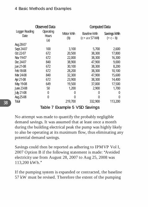
After retrofit, kWh computations were made continuously by the data logger, as well as motor operating hours. Accumulated kWhs and operating hours shown on the data logger were recorded by hand once a month as shown in Table 7, below. In this table, the savings computation is shown, relative to the constant baseline of 57 kW.


38

Observed Data Computed Data Logger Reading

Date Operating

Hours (a)

Motor kWh (b)

Baseline kWh (c = a x 57 kW)

Savings kWh (= c – b)

Aug 28-07 Sept 24-07 100 3,100 5,700 2,600 Oct 22-07 672 20,500 38,300 17,800 Nov 19-07 672 22,000 38,300 16,300 Dec 24-07 840 38,900 47,900 9,000 Jan 21-08 672 30,100 38,300 8,200 Feb 18-08 672 28,200 38,300 10,100 Mar 24-08 840 32,300 47,900 15,600 Apr 21-08 672 23,900 38,300 14,400 May 19-08 649 19,500 37,000 17,500 June 23-08 50 1,200 2,900 1,700 July 21-08 0 0 0 0 Aug 25-08 0 0 0 0 Total 219,700 332,900 113,200

Table 7 Example 5 VSD Savings

No attempt was made to quantify the probably negligible demand savings. It was assumed that at least once a month during the building electrical peak the pump was highly likely to also be operating at its maximum flow, thus eliminating any potential demand savings.

Savings could then be reported as adhering to IPMVP Vol I, 2007 Option B if the following statement is made: ‘‘Avoided electricity use from August 28, 2007 to Aug 25, 2008 was 113,200 kWh.’’

If the pumping system is expanded or contracted, the baseline 57 kW must be revised. Therefore the extent of the pumping


39

system must be recorded for the baseline period and reviewed annually during the savings reporting period.

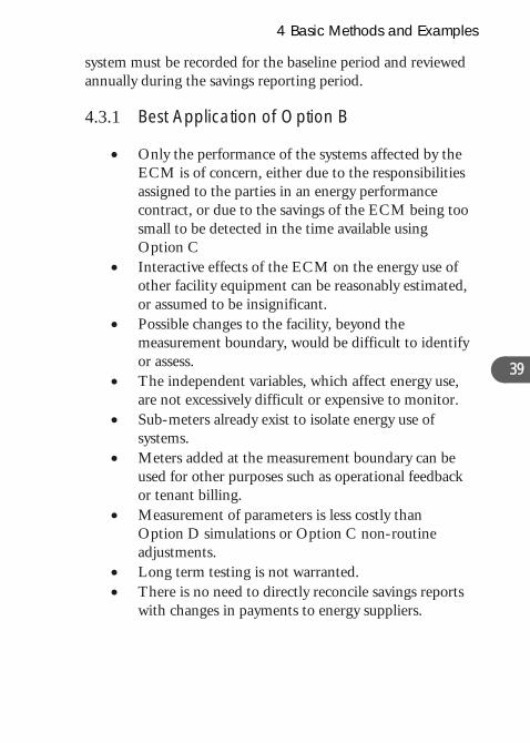
4.3.1 Best Application of Option B

• Only the performance of the systems affected by the ECM is of concern, either due to the responsibilities assigned to the parties in an energy performance contract, or due to the savings of the ECM being too small to be detected in the time available using Option C

• Interactive effects of the ECM on the energy use of other facility equipment can be reasonably estimated, or assumed to be insignificant.

• Possible changes to the facility, beyond the measurement boundary, would be difficult to identify or assess.

• The independent variables, which affect energy use, are not excessively difficult or expensive to monitor.

• Sub-meters already exist to isolate energy use of systems.

• Meters added at the measurement boundary can be used for other purposes such as operational feedback or tenant billing.

• Measurement of parameters is less costly than Option D simulations or Option C non-routine adjustments.

• Long term testing is not warranted. • There is no need to directly reconcile savings reports

with changes in payments to energy suppliers.


40

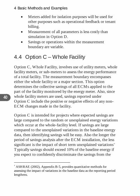
• Meters added for isolation purposes will be used for other purposes such as operational feedback or tenant billing.

• Measurement of all parameters is less costly than simulation in Option D.

• Savings or operations within the measurement boundary are variable.

4.4 Option C – Whole Facility

Option C, Whole Facility, involves use of utility meters, whole facility meters, or sub-meters to assess the energy performance of a total facility. The measurement boundary encompasses either the whole facility or a major section. This option determines the collective savings of all ECMs applied to the part of the facility monitored by the energy meter. Also, since whole facility meters are used, savings reported under Option C include the positive or negative effects of any non-ECM changes made in the facility.

Option C is intended for projects where expected savings are large compared to the random or unexplained energy variations which occur at the whole-facility level. If savings are large compared to the unexplained variations in the baseline energy data, then identifying savings will be easy. Also the longer the period of savings analysis after the ECM installation, the less significant is the impact of short term unexplained variations4. Typically savings should exceed 10% of the baseline energy if you expect to confidently discriminate the savings from the

4 ASHRAE (2002), Appendix B-5, provides quantitative methods for assessing the impact of variations in the baseline data as the reporting period lengthens.


41

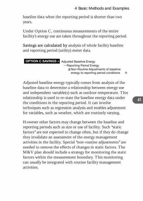
baseline data when the reporting period is shorter than two years.

Under Option C, continuous measurements of the entire facility’s energy use are taken throughout the reporting period.

Savings are calculated by analysis of whole facility baseline and reporting period (utility) meter data.

Adjusted baseline energy typically comes from analysis of the baseline data to determine a relationship between energy use and independent variable(s) such as outdoor temperature. This relationship is used to re-state the baseline energy data under the conditions in the reporting period. It can involve techniques such as regression analysis and enables adjustment for variables, such as weather, which are routinely varying.

However other factors may change between the baseline and reporting periods such as size or use of facility. Such ‘‘static factors’’ are not expected to change often, but if they do change they invalidate an assessment of the energy management activities in the facility. Special ‘‘non-routine adjustments’’ are needed to remove the effects of changes in static factors. The M&V plan should include a strategy for monitoring the static factors within the measurement boundary. This monitoring can usually be integrated with routine facility management activities.


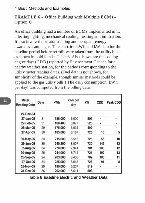
EXAMPLE 6 -- Office Building with Multiple ECMs -- Option C

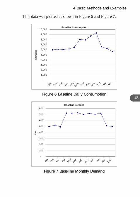
An office building had a number of ECMs implemented in it, affecting lighting, mechanical cooling, heating and infiltration. It also involved operator training and occupant energy awareness campaigns. The electrical kWh and kW data for the baseline period before retrofit were taken from the utility bills as shown in bold font in Table 8. Also shown are the cooling degree days (CDD) reported by Environment Canada for a nearby weather station, for the periods corresponding to the utility meter reading dates. (Fuel data is not shown, for simplicity of the example, though similar methods could be applied to the gas utility bills.) The daily consumption (kWh per day) was computed from the billing data.

42

Table 8 Baseline Electric and Weather Data


43

This data was plotted as shown in Figure 6 and Figure 7.

Baseline Consumption

-

1,000

2,000

3,000

4,000

5,000

6,000

7,000

8,000

9,000

10,000

Jan

Feb

Mar Apr MayJu

ne July

AugSep

tOct

Nov Dec

kWh/

day

Figure 6 Baseline Daily Consumption

Baseline Demand

-

100

200

300

400

500

600

700

800

Jan

Feb

Mar Apr MayJu

ne July

AugSep

tOct

Nov Dec

kW

Figure 7 Baseline Monthly Demand


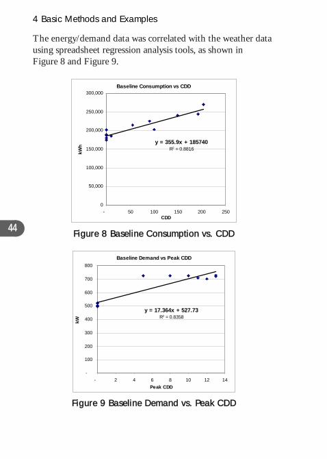
The energy/demand data was correlated with the weather data using spreadsheet regression analysis tools, as shown in Figure 8 and Figure 9.

Baseline Consumption vs CDD

y = 355.9x + 185740R2 = 0.8816

0

50,000

100,000

150,000

200,000

250,000

300,000

- 50 100 150 200 250

kWh

CDD 44 Figure 8 Baseline Consumption vs. CDD

Baseline Demand vs Peak CDD

y = 17.364x + 527.73R2 = 0.8358

-

100

200

300

400

500

600

700

800

- 2 4 6 8 10 12 14Peak CDD

kW

Figure 9 Baseline Demand vs. Peak CDD


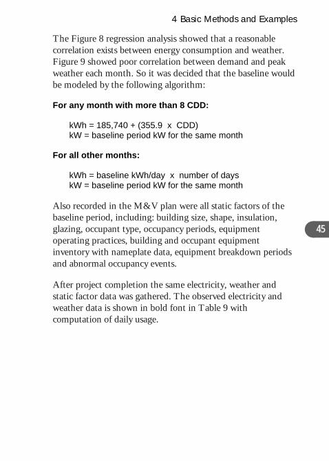
The Figure 8 regression analysis showed that a reasonable correlation exists between energy consumption and weather. Figure 9 showed poor correlation between demand and peak weather each month. So it was decided that the baseline would be modeled by the following algorithm:

For any month with more than 8 CDD:

kWh = 185,740 + (355.9 x CDD) kW = baseline period kW for the same month

For all other months:

kWh = baseline kWh/day x number of days kW = baseline period kW for the same month

Also recorded in the M&V plan were all static factors of the baseline period, including: building size, shape, insulation, glazing, occupant type, occupancy periods, equipment operating practices, building and occupant equipment inventory with nameplate data, equipment breakdown periods and abnormal occupancy events.

45

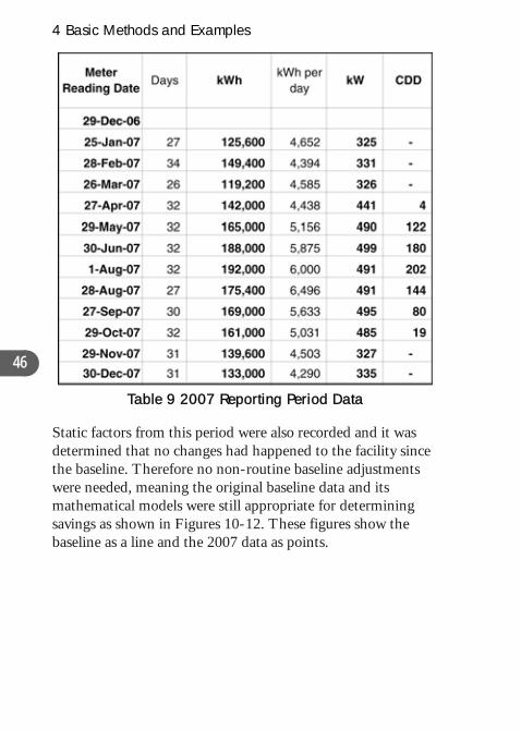
After project completion the same electricity, weather and static factor data was gathered. The observed electricity and weather data is shown in bold font in Table 9 with computation of daily usage.


46

Table 9 2007 Reporting Period Data

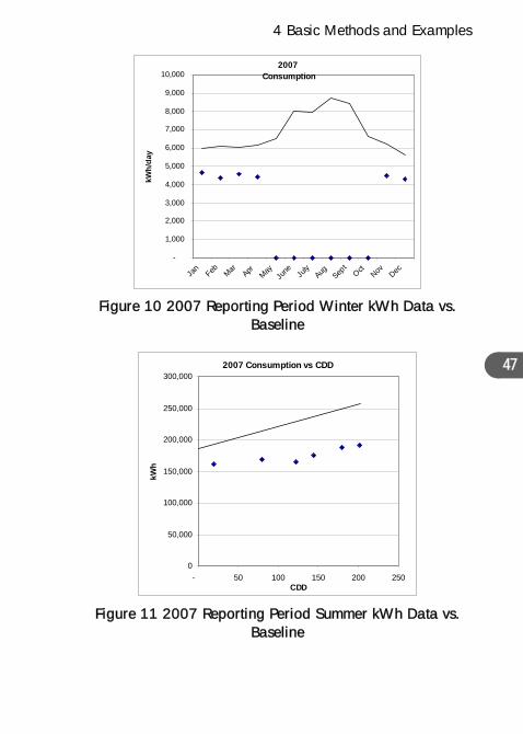
Static factors from this period were also recorded and it was determined that no changes had happened to the facility since the baseline. Therefore no non-routine baseline adjustments were needed, meaning the original baseline data and its mathematical models were still appropriate for determining savings as shown in Figures 10-12. These figures show the baseline as a line and the 2007 data as points.


47

2007 Consumption

-

1,000

2,000

3,000

4,000

5,000

6,000

7,000

8,000

9,000

10,000

Jan

Feb Mar Apr MayJu

ne July

Aug Sept

OctNov Dec

kWh/

day

Figure 10 2007 Reporting Period Winter kWh Data vs.

Baseline

2007 Consumption vs CDD

0

50,000

100,000

150,000

200,000

250,000

300,000

- 50 100 150 200 250CDD

kWh

Figure 11 2007 Reporting Period Summer kWh Data vs.

Baseline


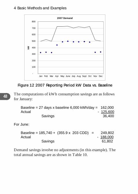
2007 Demand

-

100

200

300

400

500

600

700

800

Jan Feb Mar Apr May June July Aug Sept Oct Nov Dec

kW

Figure 12 2007 Reporting Period kW Data vs. Baseline

The computations of kWh consumption savings are as follows for January:

48

Baseline = 27 days x baseline 6,000 kWh/day = 162,000 Actual - 125,600

Savings 36,400

For June:

Baseline = 185,740 + (355.9 x 203 CDD) = 249,802 Actual - 188,000

Savings 61,802

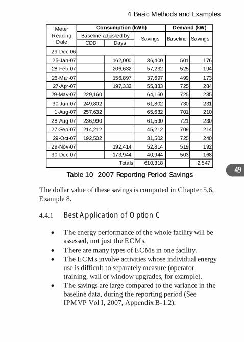
Demand savings involve no adjustments (in this example). The total annual savings are as shown in Table 10.


49

W)

29-

25 17628 194

26- 17327 284

29- 235

30 2311- 210

28- 23027- 214

29 24029-Nov-07 192,414 52,814 519 19230-Dec-07 173,944 40,944 503 168

2,547

ings

MeRe

Consumption (kWh) Demand (kBaseline adjusted by:

CDD DaysDec-06

-Jan-07 162,000 36,400 501-Feb-07 206,632 57,232 525

Mar-07 156,897 37,697 499-Apr-07 197,333 55,333 725May-07 229,160 64,160 725

-Jun-07 249,802 61,802 730Aug-07 257,632 65,632 701

Aug-07 236,990 61,590 721Sep-07 214,212 45,212 709

-Oct-07 192,502 31,502 725

SavBaselineSavings

ter ading

Date

610,318 Totals Table 10 2007 Reporting Period Savings

The dollar value of these savings is computed in Chapter 5.6, Example 8.

4.4.1 Best Application of Option C

• The energy performance of the whole facility will be assessed, not just the ECMs.

• There are many types of ECMs in one facility. • The ECMs involve activities whose individual energy

use is difficult to separately measure (operator training, wall or window upgrades, for example).

• The savings are large compared to the variance in the baseline data, during the reporting period (See IPMVP Vol I, 2007, Appendix B-1.2).


• When Retrofit Isolation techniques (Option A or B) are excessively complex. For example, when interactive effects or interactions between ECMs are substantial.

• Major future changes to the facility are not expected during the reporting period.

• A system of tracking static factors can be established to enable possible future non-routine adjustments.

• Reasonable correlations can be found between energy use and other independent variables.

4.5 Option D – Calibrated Simulation

Savings are determined through simulation of the energy use of the whole facility, or of a sub-facility.

Simulation routines are demonstrated to adequately model actual energy performance measured in the facility, (i.e. they are ‘calibrated’).

50

This Option usually requires considerable skill in calibrated simulation.

Savings are calculated by energy use simulation, calibrated with hourly or monthly utility billing data. (Energy end use metering may be used to help refine input data.)

OPTION D SAVINGS = Baseline energy from the calibrated model (without ECMs) - Actual reporting (or calibration) period energy (with ECMs) ± Calibration error in the corresponding calibration reading 5)

Simulation software is used predict energy use of a facility under a known set of conditions for which actual


(‘‘calibration’’) energy use data is also available. The simulation is adjusted to come as close to the calibration data as possible. ‘‘Calibration error’’ is the set of differences between the modeled and calibration actual data points.

Typical Applications: Multifaceted energy management program affecting many systems in a facility and where no meter or facility existed in the baseline period.

Energy use measurements, after installation of gas and electric meters, are used to calibrate a simulation.

Baseline energy use, determined using the calibrated simulation, is compared to a simulation of reporting period energy use.

EXAMPLE 7 -- New Building Designed To Be Better Than Code -- Option D 51

A new building was designed to use less energy than required by the local building code. In order to qualify for a government incentive payment, the owner was required to show that the building’s energy use during the first year of operation after commissioning and full occupancy was less than 60% of what it would have been if it had been built to code.

Computer simulation was used extensively throughout the building design process to help meet a target energy use equal to 50% of code.

The building was built as the new corporate headquarters for a large firm. It was expected that the building would become fully occupied immediately after opening.


52

The owner wished to use the same energy savings calculations that he presents to the government to show how much money was being saved as a result of his extra investment in an efficient building. He also wished to annually review variances from his initially achieved energy performance.

Option D will be used to demonstrate the new building’s savings in its first full year compared to an identical building built to building code standards. Following the first year of full operation (‘‘year one’’), year one’s energy and operational data will become the baseline for an Option C approach to reporting ongoing performance.

A year after commissioning and full occupancy, the original design simulation’s input data was updated to reflect the as-built equipment and the current occupancy. A weather data file was chosen from available weather files for the building’s location based on the file’s similarity of total heating and cooling degree days with year one’s measured degree days. This similar file was appropriately adjusted to year one’s actual monthly heating and cooling degree days. The revised input data was used to rerun the simulation.

The utility consumption data from year one was compared to this simulation model. After some further revisions to the simulation’s input data, it was deemed that the simulation reasonably modeled the current building. This calibrated simulation was called the ‘‘as-built model.’’

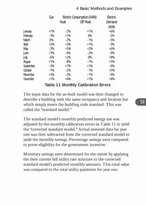
The calibration error in the as-built model relative to actual utility data is shown in Table 11.


53

Electric Consumption (kWh) Gas Peak Off Peak

Electric Demand

(kW) January +1% - 2% +1% +6% February - 3% +1% 0% - 2% March 0% - 2% - 1% - 5% April +2% +3% +1% - 3% May - 2% +5% +2% +6% June +7% - 6% - 2% - 9% July - 6% +2% 0% +8% August +1% - 8% - 1% +5% September - 3% +7% +1% - 6% October - 1% - 2% - 1% +5% November +3% - 2% - 1% - 9% December +1% +4% +1% +4%

Table 11 Monthly Calibration Errors

The input data for the as-built model was then changed to describe a building with the same occupancy and location but which simply meets the building code standard. This was called the ‘‘standard model.’’

The standard model’s monthly predicted energy use was adjusted by the monthly calibration errors in Table 11 to yield the ‘‘corrected standard model.’’ Actual metered data for year one was then subtracted from the corrected standard model to yield the monthly savings. Percentage savings were computed to prove eligibility for the government incentive.

Monetary savings were determined for the owner by applying the then current full utility rate structure to the corrected standard model’s predicted monthly amounts. This total value was compared to the total utility payments for year one.


54

The year one energy data became the basis for an Option C approach for subsequent years.

4.5.1 Best Application of Option D

• The Option D is usually used where no other Option is feasible.

• Either baseline energy data or reporting period energy data, but not both, are unavailable or unreliable. Such situation often arises in multiple building campuses (such as universities). They often have only central utility metering, i.e. no metering at individual buildings where a group of retrofits are installed. To avoid having to wait a year to gather baseline data from a new submeter at a target building, Option D might be used. A building submeter installed during the retrofit produces data during the first year after retrofit which is used to calibrate a simulation of the post retrofit situation. This calibrated simulation is then used to simulate baseline conditions and energy use so that savings can be determined by subtraction.

• There are too many ECMs to assess using Options A or B.

• The ECMs involve diffuse activities, which cannot easily be isolated from the rest of the facility, such as operator training or wall and window upgrades.

• The performance of each ECM will be estimated individually within a multiple-ECM project, but the costs of Options A or B are excessive.

• Interactions between ECMs or ECM interactive effects are complex, making the isolation techniques of Options A and B impractical. This situation


55

particularly arises in process industries. Such plants often use mass flow and energy simulation software that has been calibrated for plant design and management. Such software may be well suited to Option D for energy savings reporting.

• Major future changes to the facility are expected during the reporting period, and there is no way to track the changes and/or account for their impact on energy use.

• An experienced energy simulation professional is able to gather appropriate input data to calibrate the simulation model.

• The facility and the ECMs can be modeled by well documented simulation software.

• Simulation software predicts metered calibration data with acceptable accuracy.

• Only one year’s performance is measured, immediately following installation and commissioning of the energy management program.

4.6 Choosing an Option

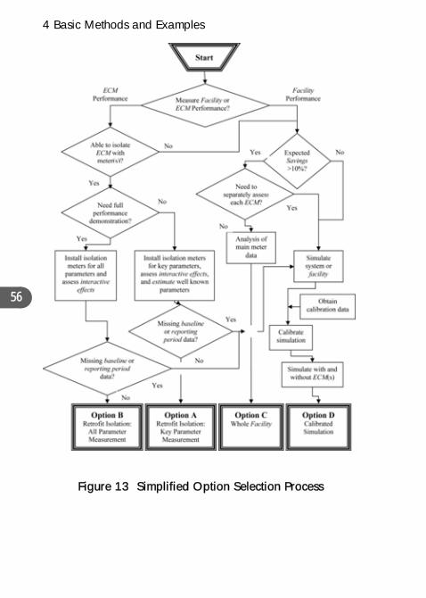
The selection between Options A, B, C or D is a decision that is made by the designer of the M&V program for each project, based on the full set of project conditions, analysis, budgets and professional judgment. Figure outlines common logic used in Option selection.

It is impossible to generalize on the best Option for any type of situation. However some key project characteristics suggest commonly favored Options as shown in Table 12 below.


56

Figure 13 Simplified Option Selection Process


57

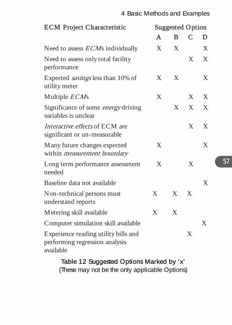
Table 12 Suggested Options Marked by ‘x’ (These may not be the only applicable Options)

Suggested Option ECM Project Characteristic A B C D

Need to assess ECMs individually X X X

Need to assess only total facility performance

X X

Expected savings less than 10% of utility meter

X X X

Multiple ECMs X X X

Significance of some energy driving variables is unclear

X X X

Interactive effects of ECM are significant or un-measurable

X X

Many future changes expected within measurement boundary

X X

Long term performance assessment needed

X X

Baseline data not available X

Non-technical persons must understand reports

X X X

Metering skill available X X

Computer simulation skill available X

Experience reading utility bills and performing regression analysis available

X


58

5 Common Issues

5 COMMON ISSUES

5.1 Baselines

Baseline information needs to be archived in the M&V plan. Such an archive, made before ECM installation, becomes the basis for accounting for changing conditions in future. It is therefore very important to ensure that the baseline record describes all energy governing aspects of the facility during the baseline period, and that it not be lost.

5.1.1 Baseline Data

Baseline information consists of energy data, independent variables, and static factors within the selected measurement boundary. Appendix A contains a full list. 59

5.1.2 Baseline Period Length

The baseline period should be established to:

• Represent all operating modes of the facility. This period should span a full operating cycle from maximum energy use to minimum. ECM planning may require study of a longer time period than is chosen for the baseline period. Longer study periods assist the planner in understanding facility performance and determining what the normal cycle length actually is.

5 Common Issues

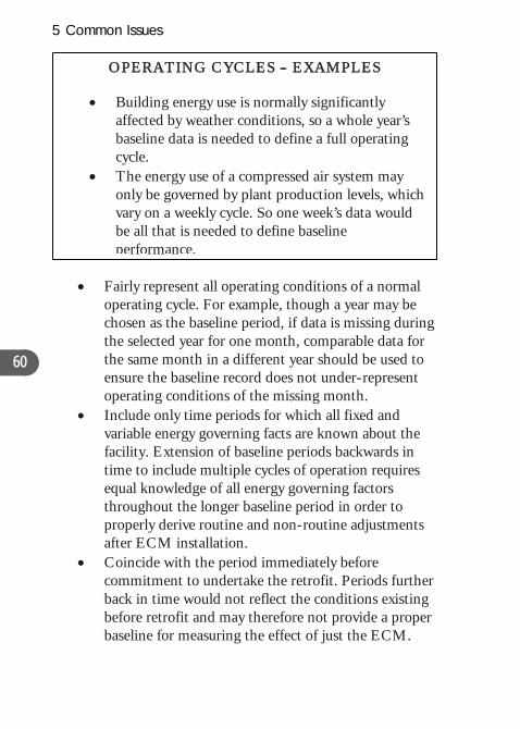
OPERATING CYCLES -- EXAMPLES

• Building energy use is normally significantly affected by weather conditions, so a whole year’s baseline data is needed to define a full operating cycle.

• The energy use of a compressed air system may only be governed by plant production levels, which vary on a weekly cycle. So one week’s data would be all that is needed to define baseline performance.

• Fairly represent all operating conditions of a normal operating cycle. For example, though a year may be chosen as the baseline period, if data is missing during the selected year for one month, comparable data for the same month in a different year should be used to ensure the baseline record does not under-represent operating conditions of the missing month.

60

• Include only time periods for which all fixed and variable energy governing facts are known about the facility. Extension of baseline periods backwards in time to include multiple cycles of operation requires equal knowledge of all energy governing factors throughout the longer baseline period in order to properly derive routine and non-routine adjustments after ECM installation.

• Coincide with the period immediately before commitment to undertake the retrofit. Periods further back in time would not reflect the conditions existing before retrofit and may therefore not provide a proper baseline for measuring the effect of just the ECM.

5 Common Issues

61

5.1.3 Baseline Adjustments

Conditions, which vary in a predictable fashion and are significant to energy use within the measurement boundary, are normally included within the mathematical model used for routine adjustments, described in Chapter 4.

Where unexpected or one-time changes occur in conditions within the measurement boundary, which are otherwise static (static factors), non-routine adjustments, also called baseline adjustments, must be made.

Non-routine adjustments are needed where a change occurs to equipment or operations within the measurement boundary after the baseline period. Such change occurs to a static factor not to independent variables. For example, an ECM improved the efficiency of a large number of light fixtures. When more light fixtures were installed, after ECM installation, a non-routine adjustment was needed to add the estimated energy of the extra fixtures to the baseline energy, so that the ECM’s true savings were still reported.

Values estimated for use in IPMVP Option A are usually chosen to eliminate the need for adjustments when changes happen within the measurement boundary. Therefore non-routine adjustments can be avoided using Option A. For example, a chiller plant’s cooling load was estimated rather than measured in order to determine Option A savings created by a chiller efficiency ECM. After retrofit, a facility addition increased the actual cooling load within the measurement boundary which consisted of just the chiller plant. However since Option A was chosen using a fixed cooling load, reported

5 Common Issues

62

savings are unchanged. The use of Option A avoided the need for a non-routine adjustment.

Baseline conditions need to be fully documented in the M&V plan so that changes in static factors can be identified and proper non-routine adjustments made. It is important to have a method of tracking and reporting changes in these same static factors. It should be established in the M&V plan who will track and report each static factor.

5.2 Measurement Equipment

Energy quantities and independent variables are measured, but we must recognize that no measurement equipment is 100% accurate. This chapter highlights some key considerations in meter accuracy. (Chapter 5.5 discusses the challenge in M&V design of balancing the costs and benefits of maintaining meter and reporting system accuracy.)

Proper meter sizing, for the range of possible quantities to be measured, ensures that collected data fall within known and acceptable error limits.

The accuracy of a meter is published by its manufacturer, from laboratory tests. Manufacturers typically rate accuracy as either a fraction of the current reading or as a fraction of the maximum reading on the meter’s scale. In this latter case it is important to consider where the typical readings fall on the meter’s scale before computing the accuracy of typical readings. Over-sizing of meters whose accuracy is stated relative to maximum reading will significantly reduce the accuracy of the actual metering.

5 Common Issues

The readings of many meter systems will ‘drift’ over time due to mechanical wear. Periodic calibration against a known standard is required to adjust for this drift.

In addition to accuracy of the meter element itself, other possibly unknown effects can reduce meter system accuracy, such as:

• poor placement of the meter so it does not get a representative ‘view’ of the quantity it is supposed to measure (e.g., a fluid flow meter’s readings are affected by proximity to an elbow in the pipe)

• data telemetry errors which randomly or systematically clip off meter data

As a result of such unquantifiable metering errors, it is important to realize that manufacturer quoted accuracy probably overstates the accuracy of the actual readings in the field. However there is no way to quantify these other effects.

63

The proper selection of meters for specific applications is a science in itself which goes beyond this guide. Chapter 7 lists some useful resources.

Utility meters are often the source of measured data for Whole Facility M&V methods (Options C and D). Since utilities maintain these meters to standards for commercial transactions, end users face no measurement challenge. However end users need to create pathways within their organization for M&V personnel to receive:

5 Common Issues

64

• copies of the utility invoices, (and understand whether a bill is based on an actual measurement or an estimate), or

• utility supplied files with all readings from multiple meters, or

• electronic pulses from a transmitter fitted to the utility’s meter (with permission).

Each of these Whole Facility issues requires planning and ongoing management to ensure the accuracy of measurements.

Retrofit Isolation methods (Options A or B) usually require more measurement effort because of the need to add special meters. These meters may be installed temporarily, such as during an energy audit to help characterize energy use before design of the ECM, and to estimate values for Option A style M&V. Or they may be installed permanently to measure baseline performance for an M&V plan, and reporting period performance.

Retrofit Isolation may require measurement of temperature, humidity, fluid flow, pressure, equipment runtime, electricity or thermal energy, for example, at the measurement boundary.

To measure electricity accurately, measure the voltage, amperage and power factor, or true rms5 wattage with a single instrument. However measurement of amperage and voltage alone can adequately define wattage in purely resistive loads, such as incandescent lamps and resistance heaters without blower motors. When measuring power, make sure that a

5 rms (root mean squared) values can be reported by solid state digital instruments to properly account for the net power when wave distortions exist in alternating current circuits.

5 Common Issues

65

resistive load’s electrical wave-form is not distorted by other devices in the facility.

Measure electric demand at the same time that the power company determines the peak demand for its billing. This measurement usually requires continuous recording of the demand at the sub-meter. From this record, the sub-meter’s demand can be read for the time when the power company reports that the peak demand occurred on its meter. The power company may reveal the time of peak demand either on its invoices or by special report (see Example 4 in Chapter 4.3).

An electrical sub-meter should measure in kVA if the utility measures in kVA.

Electric demand measurement methods vary amongst utilities. The method of measuring electric demand on a sub-meter should replicate the method the power company uses for the relevant billing meter. For example, if the power company calculates peak demand using fixed 15 minute intervals, then the recording meter should be set to record data for the same 15 minute intervals. However if the power company uses a moving interval to record electric demand data, the data recorder should have similar capabilities. Such moving interval capability can be emulated by recording data on one minute fixed intervals and then recreating the power company’s intervals using post-processing software. However, care should be taken to ensure that the facility does not contain unusual combinations of equipment that generate high one minute peak loads which may show up differently in a moving interval than in a fixed interval. After processing the data into power company intervals, convert it to hourly data for archiving and further analysis.

5 Common Issues

66

Meters should be calibrated as recommended by the manufacturer, and following procedures of recognized measurement authorities. Sensors and metering equipment should be selected based in part on the ease of calibration and the ability to hold calibration.

No data collection process is without error. It is important to be prepared for data errors or losses by designing data screening techniques to notice gaps or errors, and by having enough time (budget) to repair damaged data.

Missing or erroneous reporting period data can be re-created by interpolation between measured data points so that savings can be calculated for each period. However baseline data consist of real facts about energy and independent variables as they existed during the baseline period. Therefore baseline data problems should not be replaced by modeled data, except when using Option D. Where baseline data is missing or inadequate, seek other real data to substitute, or change the baseline period so that it contains only real data. The M&V plan should document the source of all baseline data.

5.3 Sampling

Measurement of only a sample of the full population of items or events is a valid way to reduce measurement costs. Sampling may be done in either a physical sense (i.e., only 2% of the lighting fixtures are measured) or a temporal sense (instantaneous measurement only once per hour rather than continuously).

Sampling creates errors because not all units under study are measured. The error is inversely proportional to the square

5 Common Issues

67

root of the number of measurements. That is, increasing the sample size by a factor ‘‘f’’ will reduce the error (improve the precision of the estimate) by a factor of , but increase the measurement cost.

The required fraction of any population that must be measured depends upon:

• the deviation found amongst measurements within the population, and

• the permissible error due to sampling.

In order for sampling to be cost effective, the measured units should be expected to be the same as the entire population. If there are two different types of units in the population, they should be grouped and sampled separately. For example, when designing a sampling program to measure the operating periods of room lighting controlled by occupancy sensors, rooms occupied more or less continuously (e.g., multiple person offices) should be separately sampled from those which are only occasionally occupied (e.g., meeting rooms).

Sampling must be carefully designed and conducted. A statistician should be consulted if sampling is used to control M&V costs.

5.4 On-Off Test

When an ECM can be turned on and off easily, baseline and reporting periods may be selected that are adjacent to each other in time. A change in control logic is an example of an ECM that can often be readily removed and reinstated without affecting the facility.

5 Common Issues

68

Such ‘‘On/Off tests’’ involve energy measurements with the ECM in effect, and then immediately thereafter with the ECM turned off so that pre-ECM (baseline) conditions return. The difference in energy use between the two adjacent measurement periods is the savings created by the ECM.

Equation 1) of Chapter 4 can be used for computing savings, without an adjustments term if all energy influencing factors are the same in the two adjacent periods.

This technique can be applied under both Retrofit Isolation and Whole-Facility Options. However measurement boundaries must be located so that it is possible to readily detect a significant difference in metered energy use when equipment or systems are turned on and off.

The adjacent periods used for the On/Off test should be long enough to represent stable operation. The periods should also cover the range of normal facility operations. To cover the normal range, the On/Off test may need to be repeated under different operating modes such as various seasons or production rates.

Take notice that ECMs which can be turned Off for such testing also risk being accidentally or maliciously turned Off when intended to be On.

5.5 Cost - Accuracy Tradeoffs

The measurement of any physical quantity includes errors because no measurement instrument is 100% accurate. Equation 1) usually involves at least two such measurement errors (baseline and reporting period energy), and whatever

5 Common Issues

69

error exists in the computed adjustments. To ensure that the resultant error (uncertainty) is acceptable to the users of a savings report, be certain to manage the errors inherent in measurement and analysis when developing and implementing the M&V plan.

Careful measurement system design and appropriate statistical analysis of error is needed to optimize M&V costs. It is feasible to quantify many uncertainty factors but usually not all of them. Therefore when planning an M&V process, report both quantifiable uncertainty factors and qualitative elements of uncertainty.

M&V costs should be appropriate for the size of expected savings, the length of the ECM payback period, and the report users’ interests in accuracy, frequency, and the duration of the reporting process. Often these costs can be shared with other objectives such as real time control, operational feedback, or tenant or departmental sub-billing. Prototype or research projects may bear a larger than normal M&V cost, for the sake of accurately establishing the savings generated by ECMs which will be repeated.

M&V budgeting should consider the ‘soft’ costs of designing and managing the meter hardware and data. Such soft costs are often far greater than the hardware costs.

Savings may be reported as simply the predicted savings, after verifying that the ECM is implemented as planned. Such ‘‘deemed savings’’ approach leaves more money to be spent on retrofits, and may be appropriate in circumstances where the prediction or achievement of savings is in little doubt. However the deemed savings approach misses the M&V

5 Common Issues

benefits listed in Chapter 1.2. Furthermore, since there are no recognized standards like IPMVP for predicting savings, there is little comfort for readers of deemed savings reports.

Commonly, since Option A involves estimates, it will involve fewer measurement points and lower cost, providing estimation and inspection costs are not unusually high. Option A methods usually have lower cost and higher uncertainty than Option B methods.

Since new measurement equipment is often involved in Options A or B, the cost of maintaining this equipment may make Option C less costly for long reporting periods. However, the costs of extra meters for Options A or B may be shared with other objectives of monitoring or cost allocation.

When multiple ECMs are installed at one site, it may be less costly to use Options C or D than to isolate and measure multiple ECMs with Options A or B.

70

Preparation of an Option D simulation model is often time consuming and costly. However, the model may have other uses such as for designing the ECMs themselves or designing a new facility.

Typically average annual M&V costs are less than 10% of the average annual savings being assessed. The acceptable level of cost or uncertainty in a savings reporting process is often a personal matter, which depends on the report reader’s desire for rigor. However reducing uncertainty requires more or better operational data which might enable fine tuning of savings and enhancement of other operational variables.

5 Common Issues

71

In determining the measurement level and associated costs, the M&V plan should consider the amount of variation in the energy use within the measurement boundary. For example, indoor lighting may use electricity fairly consistently all year, making it relatively easy to determine savings, while heating and cooling loads change seasonally making savings identification more difficult.

Consider the following general guidelines for balancing cost and uncertainty in an M&V process.

• Low Energy Variation & Low-Value ECM. Low-value ECMs cannot typically afford much M&V, based on the 10%-of-savings guideline above, especially if there is little variation in the measured energy data. Such combined situations would tend to favour use of Option A, and short reporting periods, for example, in the case of a constant speed exhaust fan motor that operates under a constant load according to a well defined schedule.

• High Energy Variation & Low-Value ECM. Low-value ECMs cannot generally afford much M&V. However with a high amount of variation in the energy data, the all-parameter measurement techniques of Option B may be needed to achieve the required uncertainty. Sampling techniques may be able to reduce Option B costs. Option C may not be suitable based on the general guidance in Chapter 4 that savings should exceed 10% of a facility’s metered use in order to be measurable.

• Low Energy Variation & High-Value ECM. With low variation in energy use, the level of uncertainty is often low, so Option A techniques may be most

5 Common Issues

72

suitable. However, since you expect high savings, small improvements in precision may have monetary rewards large enough to merit more precise metering and data analysis, if you can keep M&V costs appropriate relative to the savings. For example, if the savings from an ECM are $1,000,000 annually, you may decide to increase the $5,000 annual M&V cost to $20,000, if it increases precision and provides more operational data. Alternatively, a high value ECM may be clearly measurable with Option C. Option C can keep M&V costs low, if simple means are used to monitor static factors to detect the need for non-routine adjustments.

• High Energy Variation & High-Value ECM. This situation allows appropriate uncertainty reduction through extensive data collection and analysis using Options A, B or D. However savings are also likely to show in the utility records, so that Option C techniques may be used with careful monitoring of static factors to detect the need for non-routine adjustments. The reporting period may have to span multiple normal cycles of facility operation.

5 Common Issues

73

5.6 Applying Energy Prices

Cost savings are determined by applying the appropriate price schedule in the following equation:

Where: Cb = Cost of the baseline energy plus any adjustments6 Cr = Cost of the reporting period energy plus any adjustments

Costs should be determined by applying the same price schedule in computing both Cb and Cr.

The price schedule of the reporting period is normally used to compute ‘‘avoided cost.’’

The price schedule should be obtained from the energy supplier. This price schedule should include all elements that are affected by metered amounts, such as consumption charges, demand charges, transformer credits, power factor, demand ratchets, fuel price adjustments, early payment discounts and taxes.

An alternative procedure for valuing savings involves multiplying energy units saved by the marginal price of energy. Be careful to ensure that the marginal price is valid for the level of consumption and demand of both the baseline and reporting periods. Such marginal pricing is usually the only way to value savings determined under Retrofit Isolation Options A or B.

6 Adjustments are the appropriate ones described in Chapter 4.

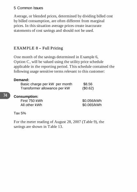
5 Common Issues

74

Average, or blended prices, determined by dividing billed cost by billed consumption, are often different from marginal prices. In this situation average prices create inaccurate statements of cost savings and should not be used.

EXAMPLE 8 -- Full Pricing

One month of the savings determined in Example 6, Option C, will be valued using the utility price schedule applicable in the reporting period. This schedule contained the following usage sensitive terms relevant to this customer:

Demand: Basic charge per kW per month $8.56 Transformer allowance per kW ($0.62)

Consumption: First 750 kWh $0.056/kWh All other kWh $0.065/kWh

Tax 5% For the meter reading of August 28, 2007 (Table 9), the savings are shown in Table 13.

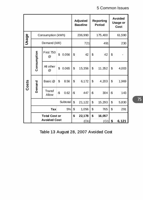
5 Common Issues

75

236,990 175,400 61,590

721 491 230

First 750 @ 0.056$ 42$ 42$ -$

All other @ 0.065$ 15,356$ 11,352$ 4,003$

Basic @ 8.56$ 6,172$ 4,203$ 1,969$

Transf Allow 0.62-$ 447-$ 304-$ 143-$

21,122$ 15,293$ 5,830$

5% 1,056$ 765$ 291$

22,178$ 16,057$ (Cb) (Cr)

Adjusted Baseline

Reporting Period

Cos

ts

Total Cost or Avoided Cost $ 6,121

Consumption (kWh)

Demand (kW)Usag

e

Con

sum

ptio

nD

eman

d

Avoided Usage or

Cost

Subtotal

Tax

Table 13 August 28, 2007 Avoided Cost

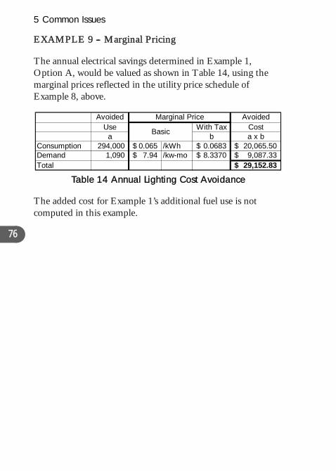
5 Common Issues

76

Avoided Marginal Price AvoidedUse With Tax Cost

a b a x bConsumption 294,000 0.065$ /kWh 0.0683$ 20,065.50$ Demand 1,090 7.94$

EXAMPLE 9 -- Marginal Pricing

The annual electrical savings determined in Example 1, Option A, would be valued as shown in Table 14, using the marginal prices reflected in the utility price schedule of Example 8, above.

/kw-mo 8.3370$ 9,087.33$ Total 29,152.83$

Basic

Table 14 Annual Lighting Cost Avoidance

The added cost for Example 1’s additional fuel use is not computed in this example.

6 Definitions

77

6 DEFINITIONS

Adjusted Baseline Energy: The energy use of the baseline period, adjusted to a different set of operating conditions.

Avoided Energy Use: The reduction in energy use that occurred in the reporting period, relative to what would have occurred if the facility had been equipped and operated as it was in the baseline period but under reporting period operating conditions. ‘‘Cost avoidance’’ is the monetary equivalent of ‘‘avoided energy use.’’ Both are commonly called savings.

Baseline Adjustments: The non-routine adjustments arising during the reporting period from changes in any energy governing characteristic of the facility within the measurement boundary, except the named independent variables used for routine adjustments.

Baseline Energy: The energy use occurring during the baseline period without adjustments.

Baseline Period: The period of time chosen to represent operation of the facility or system before implementation of an ECM. This period may be as short as the time required for an instantaneous measurement of a constant quantity, or long enough to reflect one full operating cycle of a system or facility with variable operations.

Baseline: Pertaining to the baseline period (see Chapter 5.1).

Constant: A term used to describe a physical parameter which does not change during a period of interest. Minor variations may be observed in the parameter while still describing it as

6 Definitions

constant. The magnitude of variations that are deemed to be ‘minor’ must be reported in the M&V plan.

Commissioning: A process for achieving, verifying and documenting the performance of equipment to meet the operational needs of the facility within the capabilities of the design, and to meet the design documentation and the owner's functional criteria, including preparation of operating personnel.

Cycle: The period of time between the start of successive similar operating modes of a facility or piece of equipment whose energy use varies in response to operating procedures or independent variables. For example the cycle of most buildings is 12 months, since their energy use responds to outdoor weather which varies on an annual basis. Another example is the weekly cycle of an industrial process which operates differently on Sundays than during the rest of the week. 78

Degree Day: A degree day is measure of the heating or cooling load on a facility created by outdoor temperature. When the mean daily outdoor temperature is one degree below a stated reference temperature such as 18oC, for one day, it is defined that there is one heating degree day. If this temperature difference prevailed for ten days there would be ten heating degree days counted for the total period. If the temperature difference were to be 12 degrees for 10 days, 120 heating degree days would be counted. When the ambient temperature is below the reference temperature it is defined that heating degree days are counted. When ambient temperatures are above the reference, cooling degree days are counted. Any reference temperature may be used for recording degree days, though it is usually chosen to reflect the

6 Definitions

79

temperature at which a particular building no longer needs heating or cooling.

Energy: Energy or demand.

Energy Conservation Measure (ECM): An activity or set of activities designed to increase the energy efficiency of a facility, system or piece of equipment. ECMs may also conserve energy without changing efficiency. An ECM may be applied as a retrofit to an existing system or facility, or as a modification to a design before construction of a new system or facility.

Estimate: A process of determining a parameter used in a savings calculation through methods other than measuring it in the baseline and reporting periods. These methods may range from arbitrary assumptions to engineering estimates derived from manufacturer’s rating of equipment performance. Equipment performance tests that are not made in the place where they are used during the reporting period are estimates, for purposes of adherence with IPMVP.

Facility: A building or industrial site containing several energy using systems. A wing or section of a larger facility can be treated as a facility of its own if it has meters which separately measure all of its energy.

Independent Variable: A parameter that is expected to change regularly and have a measurable impact on the energy use of a system or facility.

Interactive Effects: Energy effects created by an ECM but not measured within the measurement boundary.

6 Definitions

Marginal Price: The cost of one additional unit of a commodity billed under a complex rate schedule.

Measurement and Verification (M&V): The process of using measurements to reliably determine actual savings created within an individual facility by an energy management program.

Measurement Boundary: A notional boundary drawn around equipment and/or systems to segregate those which are relevant to savings determination from those which are not. See Chapter 4.1.

Metering: Collection of energy data over time at a facility through the use of measurement devices.

M&V Plan: The document defined in Appendix A. 80

Non-Routine Adjustments: The individually engineered calculations in Equation 1) of Chapter 4 to account for changes in static factors within the measurement boundary since the baseline period. When non-routine adjustments are applied to the baseline energy they are sometimes called just ‘‘baseline adjustments.’’ (See also Chapter 5.1.)

Proxy: A measured parameter substituted in place of direct measurement of an energy parameter, where a relationship between the two has been proven on site. For example, if a relationship has been proven between the output signal from a variable speed drive controller and the power requirements of the controlled fan, this output signal is a proxy for fan power.

Regression Analysis: A mathematical technique that extracts parameters from a set of data to describe the correlation of

6 Definitions

measured independent variables and dependent variables (usually energy data).

Reporting Period: The period of time following implementation of an ECM when savings reports adhere to IPMVP. This period may be as short as the time for an instantaneous measurement of a constant quantity; long enough to reflect all normal operating modes of a system or facility with variable operations; the length of the financial payback period for an investment; the duration of a performance measurement period under an energy performance contract; or indefinite.

Routine Adjustments: The calculations in Equation 1) of Chapter 4 made by a formula shown in the M&V plan to account for changes in selected independent variables within the measurement boundary since the baseline period.

81Savings: The reduction in energy use or cost commonly expressed as avoided energy use or cost. Savings, as used in IPMVP, are not the simple difference between baseline and reporting period utility bills or metered quantities. See Chapter 4 for elaboration on this point.

Simulation Model: An assembly of algorithms that calculates energy use for a facility based on engineering equations and user-defined parameters.

Static Factors: Those characteristics of a facility which affect energy use, within the chosen measurement boundary, but which are not used as the basis for any routine adjustments. These characteristics include fixed, environmental, operational and maintenance characteristics. They may be constant or varying.

6 Definitions

82

7 Other Resources

83

7 OTHER RESOURCES

INTERNATIONAL PERFORMANCE MEASUREMENT AND VERIFICATION PROTOCOL (IPMVP)

Available at www.evo-world.org.

• Volume I, Concepts and Options for Determining Energy and Water Savings, 2007. Key elements are included in this guide, with permission.

• Volume II, Concepts and Practices for Improved Indoor Environmental Quality, 2002. Presentation of the potential interactions between energy efficiency activities and indoor environmental quality. Guidance on measurement of indoor environmental quality for purposes of tracking changes in conditions from those of the baseline period.

• Volume III, Part 1, Concepts and Practices for Determining Energy Savings in New Construction, 2006. Application of Volume I concepts to the assessment of performance of a new building relative to a notional baseline.

• Volume III, Part II, Concepts and Practices for Determining Energy Savings in Renewable Energy Technologies Applications, 2003. Application of Volume I concepts to the assessment of performance of renewable technologies behind the utility meter.


7 Other Resources

84

ASHRAE GUIDELINE 14 Measurement of Energy and Demand Savings, 2002 (Under revision). Available at www.ashrae.org. Contains many concepts similar to those in IPMVP, with more technical details. It requires an uncertainty statement with each savings report except for a specific set of circumstances for Whole Facility savings reports. It includes useful information on sensors, calibration techniques, lab standards for measurement, and test methods for chillers, fans, pumps, motors, boilers, furnaces, thermal storage and air handling systems.

BRITISH COLUMBIA HYDRO, Stepped Rate Impact Study Guidelines, Methods for Determining Energy Savings for Power Smart Projects, 2006. This document, available from Ken Lau at [email protected] defines requirements for major industrial power users to benefit from a conservation oriented rate incentive program. Uses some IPMVP concepts, but also allows savings reports without field measurements for situations where the variables are adequately known beforehand.

UNITED STATES DEPARTMENT OF ENERGY, FEDERAL ENERGY MANAGEMENT PROGRAM, M&V Guidelines: Measurement and Verification for Federal Energy Projects Version 3.0, 2008. Available at http://www1.eere.energy.gov/femp/pdfs/mv_guidelines.pdf. Contains many concepts similar to those in IPMVP. It includes specific M&V design details that are allowed for some common ECMs in federal government buildings.

http://www.ashrae.org/

mailto:[email protected]

http://www1.eere.energy.gov/femp/pdfs/mv_guidelines.pdf

7 Other Resources

85

INTERNET SITES with resources and links to other useful sites:

• http://www.evo-world.org • http://ateam.lbl.gov/mv/


http://ateam.lbl.gov/mv/

7 Other Resources

86

Appendix A: Contents of a Full M&V Plan

87

APPENDIX A: CONTENTS OF A FULL M&V PLAN

A complete M&V plan should include discussion of the following 13 topics:

1. ECM Intent -- Describe the ECM, its intended result, and the commissioning procedures that will be used to verify successful implementation of each ECM. Identify any planned changes to conditions of the baseline, such as unoccupied building temperature settings.

2. Selected IPMVP Option and Measurement Boundary -- Specify which IPMVP Option, defined in Chapters 4.2 -- 4.5, will be used to determine savings. This identification should include the date of publication or the version number and Volume number of the IPMVP edition being followed (IPMVP Volume I EVO 10000-1:2007), for example). Identify the measurement boundary of the savings determination. The boundary may be as narrow as the flow of energy through a pipe or wire, or as broad as the total energy use of one or many buildings. Describe the nature of any interactive effects beyond the measurement boundary together with their possible effects.

3. Baseline: Period, Energy and Conditions --Document

the facility’s baseline conditions and energy data, within the measurement boundary. (In energy performance contracts, baseline energy and baseline conditions may be


88

defined by either the owner or the ESCO, providing the other party is given adequate opportunity to verify them.)

An energy audit used for establishing the objectives of a savings program or terms of an energy performance contract usually provides most if not all of the baseline documentation needed in the M&V plan. This baseline documentation should include:

a) Identification of the baseline period b) All baseline energy consumption and demand data c) All independent variable data coinciding with the

energy data (e.g. production rate, ambient temperature)

d) All static factors coinciding with the energy data: • Occupancy type, density and periods • Operating conditions for each baseline operating

period and season, other than the independent variables. (For example, in an industrial process, baseline operating conditions might include product type(s), raw material type, and number of production shifts per day. In a building, baseline operating conditions might include light level, space temperature humidity and ventilation levels. An assessment of thermal comfort and/or indoor air quality (IAQ) may also prove useful in cases where the new system performs differently than the old inefficient system. See IPMVP Volume II.)

• Description of any baseline conditions that fall short of required conditions. For example, the space is under-heated during the baseline, but the ECM will restore the desired temperature. Details


89

of all adjustments that are necessary to the baseline energy data to reflect the energy management program’s expected improvement from baseline conditions.

• Size, type, and insulation of any relevant building envelope elements such as walls, roofs, doors, windows.

• Equipment inventory: nameplate data, location, condition. Photographs or videotapes are effective ways to record equipment condition.

• Equipment operating practices (schedules and setpoints, actual temperatures and pressures)

• Significant equipment problems or outages during the baseline period.

The baseline documentation typically requires well documented audits, surveys, inspections and/or short term metering activities. The extent of this information is determined by the measurement boundary chosen or the scope of the savings determination.

Where whole facility M&V methods are employed (Chapter 4.4), all facility equipment and conditions should be documented.

4. Reporting Period -- Identify the reporting period. This period may be as short as an instantaneous measurement during commissioning of an ECM, or as long as the time required to recover the investment cost of the ECM program.

5. Basis for Adjustment -- Declare the set of conditions to which all energy measurements will be adjusted. The


90

conditions are usually those of the reporting period. However IPMVP describes a process for reporting savings under some other set of fixed conditions.

6. Analysis Procedure -- Specify the exact data analysis

procedures, algorithms and assumptions to be used in each savings report. For each mathematical model used, report all of its terms and the range of independent variables over which it is valid.

7. Energy Prices -- Specify the energy prices that will be used to value the savings, and whether and how savings will be adjusted if prices change in future (see Chapter 5.6).

8. Meter Specifications -- Specify the metering points, and

period(s) if metering is not continuous. For non-utility meters, specify: meter characteristics, meter reading and witnessing protocol, meter commissioning procedure, routine calibration process, and method of dealing with lost data (see Chapter 5.2).

9. Monitoring Responsibilities -- Assign responsibilities for

reporting and recording the energy data, independent variables and static factors within the measurement boundary during the reporting period.

10. Expected Accuracy -- Evaluate the expected accuracy

associated with the measurement, data capture, sampling and data analysis. This assessment should include qualitative and any feasible quantitative measures of the level of uncertainty in the measurements and adjustments to be used in the planned savings report (see Chapter 5.5).


91

11. Budget -- Define the budget and the resources required

for the savings determination, both initial setup costs and ongoing costs throughout the reporting period.

12. Report Format -- Specify how results will be reported and

documented (see Appendix B). A sample of each report should be included.

13. Quality Assurance -- Specify quality assurance procedures

that will be used for savings reports and any interim steps in preparing the reports.

Depending upon the circumstances of each project, some additional specific topics should also be discussed in a complete M&V plan:

For Option A:

• Justification of Estimates -- Report the values to be used for all estimated values. Explain the source of these estimated values. Show the overall significance of these estimates to the total expected savings by reporting the range of the possible savings associated with the range of plausible values of the estimated parameters.

• Periodic Inspections -- Define the periodic inspections that will be performed in the reporting period to verify that equipment is still in place and operating as assumed when determining the estimated values.


92

For Option D:

• Software Name -- Report the name and version number of the simulation software to be used.

• Input/Output Data -- Provide a paper and electronic copy of the input files, output files, and weather files used for the simulation.

• Measured Data -- Note which input parameters were measured and which were estimated. Describe the process of obtaining any measured data.

• Calibration -- Report the energy and operating data used for calibration. Report the accuracy with which the simulation results match the calibration energy data.

Where the nature of future changes can be anticipated, define methods for making the relevant non-routine adjustments.

Time and budget requirements (item 11, above) are often underestimated, which ultimately leads to incomplete data collection. A less accurate and less expensive savings determination is better than an incomplete or poorly done determination, which is theoretically more accurate but under-funded. Chapter 5.5 addresses cost-accuracy tradeoffs.

Appendix B: Contents of a Full Energy Savings Report

93

APPENDIX B: CONTENTS OF A FULL ENERGY SAVINGS REPORT

Complete savings reports should include at least:

• Observed data of the reporting period: o the measurement period start and end points

in time, o the energy data, and o the values of the independent variables.

• Description and justification for any corrections made to observed data

• For Option A the agreed estimated values • Energy price schedule used • All details of any baseline non-routine adjustment

performed. Details should include: o an explanation of the change in conditions

since the baseline period, o all observed facts and assumptions, and o the engineering calculations leading to the

adjustment. • Computed savings in energy and monetary units.

All reporting should follow the M&V plan.

Appendix B: Contents of a Full Energy Savings Report

94

Your feedback and comments are appreciated. Please provide suggestions to:

[email protected]

Energy Efficiency is Good Business • Economic Prosperity

• Environmental Performance

• Social Responsibility

• Security

7031 energy savings measurement guide - ceati ... · energy savings measurement guide. following...

Documents