8. MODELING TRACE METALS

Art is the lie that helps us to see the truth.

- Pablo Picasso

8.1 INTRODUCTION

Modeling is a little like art in the words of Pablo Picasso. It is never completely realistic; it is never the truth. But it contains enough of the truth, hopefully, and enough realism to gain understanding about environmental systems.

Improvements in analytical quantitation have affected markedly the basis for governmental regulation of trace metals and increased the importance of mathematical modeling.

Figure 8.1 was compiled from manufacturers‘ literature on detection limits for lead in water samples. As we changed from using wet chemical techniques for lead analysis (1950-l960), to flame atomic absorption (1960-1975), to graphite furnace atomic absorption (1975-l990), to inductively coupled plasma mass spectrometry with preconcentration (1985-present), the limit of detection has improved from approximately 10-5 (10 mg L-1) to 10-l2 (1.0 ng L-1).

In some cases, water quality standards have become more stringent when there are demonstrated effects at low concentrations.

Some perspective on Figure 8.1 is provided by Table 1.3. Drinking water standards are given in Table 8.1 for metals and inorganic chemicals.

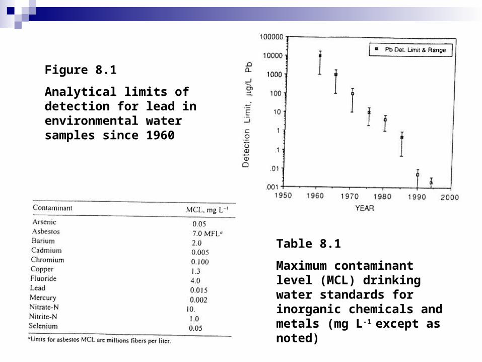
Figure 8.1

Analytical limits of detection for lead in environmental water samples since 1960

Table 8.1

Maximum contaminant level (MCL) drinking water standards for inorganic chemicals and metals (mg L-1 except as noted)

"Heavy metals" usually refer to those metals between atomic number 21 (scandium) and atomic number 84 (polonium), which occur either naturally or from anthropogenic sources in natural waters. These metals are sometimes toxic to aquatic organisms depending on their concentration and chemical speciation.

Heavy metals differ from xenobiotic organic pollutants in that they frequently have natural background sources from dissolution of rocks and minerals. The mass of total meta1 is conservative in the environment; although the pollutant may change its chemical speciation, the total remains constant.

Heavy metals are a serious pollution problem when their concentration exceeds water quality standards. Thus waste load allocations are needed to determine the permissible discharges of heavy metals by industries and municipalities.

In addition, volatile metals (Cd, Zn, Hg, Pb) are emitted from stack gases, and fly ashes contain significant concentrations of As, Se, and Cr, all of which can be deposited to water and soil by dry deposition.

8.1.1 Hydrolysis of Metals

All metal cations in water are hydrated, that is, they form aquo complexes with H2O.

The number of water molecules that are coordinated around a water is usually four or six. We refer to the metal ion with coordinated water molecules as the “free aquo metal ion”.

The analogous situation is when one writes H+ rather than H3O+ for a proton in water; the coordination number is one for a proton.

The acidity of H2O molecules in the hydration shell of a metal ion is much larger than the bulk water due to the repulsion of protons in H2O molecules by the + charge of the metal ion.

Trivalent aluminum ions (monomers) coordinate six waters. Al3+ is quite acidic,

(1) because the charge to ionic radius ratio of A13+ is large. Al3+ · 6 H2O can als

o be written as Al(H2O)3+6

The maximum coordination number or metal cations for ligands in solution is usually two times its charge. Metal cations coordinate 2, 4, 6, or sometimes 8 ligands. Copper (II) is an example of a metal cation with a maximum coordination number of 4.

(2)

(3) Metal ions can hydrolyze in solution, demonstrating their acidic property. This

discussion follows that of Stumm and Morgan. (4) Equation (4) can be written more succinctly below.

(5)

Kl is the equilibrium constant, the first acidity constant. If hydrolysis leads to supersaturated conditions or metal ions with respect to th

eir oxide or hydroxide precipitates, thus: (6)

Formation or precipitates can be considered as the final stage of polynuclear complex formation:

(7)

8.1.2 Chemical Speciation

Speciation of metals determines their toxicity. Often, free aguo metal ions are toxic to aquatic biota and the complexed metal ion is not. Chemical speciation also affects the relative degree of adsorption or binding to particles in natural waters, which affects its fate (sedimentation, precipitation, volatilization) and toxicity.

Figure 8.2 is a periodic chart that has been abbreviated to emphasize the chemistry of metals into two categories of behavior: A-cations (hard) or B-cations (soft).

The classification of A- and B-type metal cations is determined by the number of electrons in the outer d orbital. Type-A metal cations have an inert gas type of arrangement with no electrons (or few electrons) in the d orbital, corresponding to "hard sphere“ cations.

Type-A metals form complexes with F- and oxygen donor atoms in ligands such as OH-, CO3

2-, and HCO32-. They coordinate more strongly with H2O

molecules than NH3 or CN-. Type-B metals (e.g., Ag+, Au+, Hg2+, Cu+, Cd2+) have many electrons in the

outer d orbital. They are not spherical, and their electron cloud is easily deformed by ligand fields.

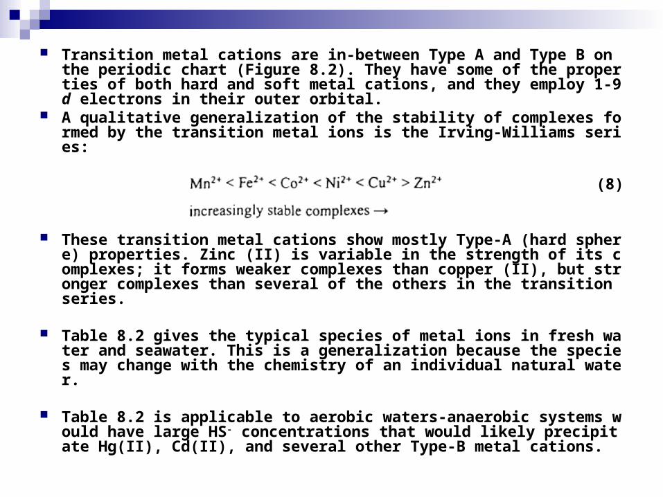
Transition metal cations are in-between Type A and Type B on the periodic chart (Figure 8.2). They have some of the properties of both hard and soft metal cations, and they employ 1-9 d electrons in their outer orbital.

A qualitative generalization of the stability of complexes formed by the transition metal ions is the Irving-Williams series:

(8)

These transition metal cations show mostly Type-A (hard sphere) properties. Zinc (II) is variable in the strength of its complexes; it forms weaker complexes than copper (II), but stronger complexes than several of the others in the transition series.

Table 8.2 gives the typical species of metal ions in fresh water and seawater. This is a generalization because the species may change with the chemistry of an individual natural water.

Table 8.2 is applicable to aerobic waters-anaerobic systems would have large HS- concentrations that would likely precipitate Hg(II), Cd(II), and several other Type-B metal cations.

Figure 8.2 Partial periodic table showing hard (A-type) metal cations and soft (B-type) metal cations

Table 8.2

Major species of metal cations in aerobic fresh water and seawater

8.1.3 Dissolved Versus Particulate Metals Heavy metals that have a tendency to form strong complexes in solution al

so have a tendency to fem surface complexes with those same ligands on particles. Difficulty arises because chemical equilibrium models must distinguish between what is actually dissolved in water versus that which is adsorbed. Analytical chemists have devised an operational definition of "dissolved constituents" as all those which pass a 0.457 µm membrane filter.

Windom et al. and Cohen have demonstrated that filtered samples can bec

ome easily contaminated in the filtration process. As per Horowitz, there are two philosophies for processing a filtered sample for quantitation of dissolved trace elements:

(1) treat the colloidally associated trace elements as contaminants and attempt to exclude them from the sample as much as possible, or

(2) process the sample in such a way that most colloids will pass the filter (large particles will not) and try to standardize the technique so that results are operationally comparable.

Shiller and Taylor and Buffle have proposed ultrafiltration, sequential flow fractionation, or exhaustive filtration as methods to approach the goal of excluding colloidally associated metals from the water sample entirely.

Flegal and Coale were among the first to report that previous trace metal data sets suffered from serious contamination problems. The modeler needs to under stand how water samples were obtained because it can affect results when simulating trace metals concentrations in the nanogram per liter range, especially.

According to Benoit, ultraclean procedures have three guiding principles: - (1) samples contact only surfaces consisting of materials that are low in metals and that have been extensively acid-cleaned in a filtered air environment; - (2) samples are collected and transported taking extraordinary care to avoid contamination from field personnel or their gear;- (3) all other sample handling steps take place in a filtered air environment and using ultra-pure reagents.

The "sediment-dependent" partition coefficient for metals (Kd) is an artifact, to large extent, of the filtration procedure in which colloid-associated trace metals pass the filter and are considered "dissolved constituents”.

8.2 MASS BAIANCE AND WASTE LOAD ALLOCATION FOR RIVERS

8.2.1 Open-Channel Hydraulics A one-dimensional model is the St. Venant equations for nonsteady, open-c

hannel flow. We must know where the water is moving before we can model the trace metal constituents.

(9)

(10)

where Q = discharge, L3T-1

t = time, T z = absolute elevation of water level above sea level, L

A = total area of cross section, L2

b = width at water level, L g = gravitational acceleration, LT-2

x = longitudinal distance, L qi = lateral inflow per unit length of river, L2T-1

Sf = the friction slope:

(11)

Only a few numerical codes that are available solve the fully dynamic open-channel flow equations. It requires detailed cross-sectional area/stage relationships, stage/discharge relationships, and stage and discharge measurements with time.

Trace metals are often associated with bed sediments, and sediment transp

ort is very nonlinear. Bed sediment is scoured during flood events when critical shear stresses at the bed-water interfaces are exceeded.

Necessary to solve the fully dynamic St. Venant equations. Equations (9) and (10) can be simplified:

(1) lateral inflow qi can be neglected and accounted for at the beginning of each stream segment;

(2) the river can be segmented into reaches where Q(x) is approximately constant within each segment;

(3) the river can be segmented into reaches where A(x) is approximately constant within each segment.

If Q and A can be approximated as constants in (x, t), then the velocity is constant and the problem reduces to one or steady flow.

8.2.2 Mass Balance Equation

Figure 8.3: a schematic of trace metal transport in a river. Metals can be in the particulate-adsorbed or dissolved phases in the sediment or overlying water column. Interchange between sorbed metal ions and aqueous metal ions occurs via adsorption/desorption mechanisms.

Bed sediment can be scoured and can enter the water column, and suspended solids can undergo sedimentation and be deposited on the bed. Metal ions in pore water of the sediment can diffuse to the overlying water column and vice versa, depending on the concentration driving force.

Under steady flow conditions (dQ/dt = 0), we can consider the time-variable concentration of metal ions in sediment and overlying water. We will assume that adsorption and desorption processes are fast relative to transport processes and that the suspended solids concentration is constant within the river segment.

Sorption kinetics are typically complete within 1 hour, which is fast compared to transport processes, except perhaps during high-flow events. Suspended solids concentrations can be assumed as constant within a segment under steady flow conditions.

The modeling approach is to couple a chemical equilibrium model with the mass balance equations for total metal concentration in the water column.

In this way, we do not have to write a mass balance equation for every che

mical species (which is impractical). The approach assumes that chemical equilibrium among metal species in solution and between phases is valid.

Acid-base reactions and complexation reactions are fast (on the order of minutes to microseconds). Precipitation and dissolution reactions can be slow; if this is the case, the chemical equilibrium submodel will flag the relevant solid phase reaction (provided that the user has anticipated the possibility).

Redox reactions can also be slow. The modeler must have some knowledge of aquatic chemistry in order to make an intelligent choice of chemical species in the equilibrium model.

Assuming local equilibrium for sorption, we may write the mass balance equations similarly to those given in Chapter 7 for toxic organic chemicals in a river. The only difference is that metals do not degrade-they may undergo chemical reactions or biologically mediated redox transformations, but the tota1 amount of metal remains unchanged.

If chemical equilibrium does not apply, each chemical species of concern must be simulated with its own mass balance equation.

An example would be the methylation and dimethylation of Hg and Hg0 volatilization, which are relatively slow processes, and chemical equilibrium would not apply.

(12)

(13)

Where CT = total whole water (unfiltered) concentration in the water column, M L-3

t = time, T A = cross sectional area, L2

Q = flowrate, L3T-1

x = longitudinal distance, L E = longitudinal dispersion coefficient, L2T-1

ks = sedimentation rate constant, T-1

fp,w = particulate adsorbed fraction in the water column, dimensionless

fd,w = dissolved chemical fraction in the water column, dimensionless

Kp,b = sediment-water distribution coefficient in the bed, L3M-1

r = adsorbed chemical in bed sediment, MM-1

kL = mass transfer coefficient between bed sediment and water column, LT-1

h = depth of the water column (stage), L α = scour coefficient of bed sediment into overlying water, T-1

Sb = bed sediment so1ids Concentration, ML-3 bed volume γ = ratio of water depth to active bed sediment layer,

dimensionless d = depth of active bed sediment, L

The model is similar to that depicted in Figure 8.3 except that we assume instantaneous sorption equilibrium in the water column and sediment between the adsorbed and dissolved chemical phases.

The first two terms of equation (12) are for advective and dispersive trans

port for the case of variable Q, E, and A with distance.

The last term in equations (12) and (13) accounts for scour of particulate adsorbed material from the bed sediment to the overlying water using a first-order coefficient for scour, α, that would depend on flow and sediment properties.

Equations (12) and (13) are a set of partial differential equations that can be solved by the method of characteristics or operator splitting methods.

This set of two equations is very powerful because it can be used to model situations when the bed is contaminated and diffusing into the overlying water or when there are point source discharges that adsorb and settle out of the water column to the bed.

Figure 8.3 Schematic model of metal transport in a stream or river showing suspended and bed load transport of dissolved and adsorbed particulate material.

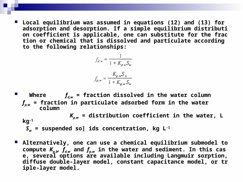
Local equilibrium was assumed in equations (12) and (13) for adsorption and desorption. If a simple equilibrium distribution coefficient is applicable, one can substitute for the fraction or chemical that is dissolved and particulate according to the following relationships:

Where fd,w = fraction dissolved in the water column

fp,w = fraction in particulate adsorbed form in the water column

Kp,w = distribution coefficient in the water, L kg-1

Sw = suspended so] ids concentration, kg L-1

Alternatively, one can use a chemical equilibrium submodel to compute Kp,

b, fd,w and fp,w in the water and sediment. In this case, several options are available including Langmuir sorption, diffuse double-layer model, constant capacitance model, or triple-layer model.

8.2.3 Waste Load Allocation

Point source discharges that continue for a long period will eventually come to steady state with respect to river water quality concentrations. The steady state will be perturbed by rainfall runoff discharge events, but the river may tend toward an "average condition”.

Under steady-state conditions (∂CT/∂t = 0 and ∂r/∂t = 0), equations (12) and (13) reduce to the following:

(14)

For large rivers, after an initial mixing period, dispersion can be estimated by Fischer's equation:

(15), (16) where g is the gravitational constant (LT-2), h is the mean depth (L), and S

is the energy slope of the channel (LL-1).

A mixing zone in the river is allowed in the vicinity of the wastewater discharge where locally high concentrations may exist before there is adequate time for mixing across the channel and with depth.

The mixing zone can be estimated from the empirical equation (17):

(17)

where Xℓ = mixing length for a side bank discharge, ft B = river width, ft

Ey = lateral dispersion coefficient, ft2 s-1 = єhu*

є = proportionality coefficient = 0.3 - 1.0

u* = shear velocity as defined in equation (16), ft s-1

h = mean depth, ft

The most basic waste load allocation is a simple dilution calculation assuming complete mixing or the waste discharge with the upstream metals concentration. One assumes that the total metal concentration (dissolved plus particulate adsorbed concentrations) are bioavailable to biota as a worst case condition.

At the next level or complexity, the waste load allocation may become a probalistic calculation using Monte Carlo analysis.

Using the following equation:

Where CT = total metals concentration, ML-3

Qu = upstream flowrate, L3T-1

Cu = upstream metals concentration, ML-3

Qw = wastewater discharge flowrate, L3T-1

Cw = wastewater metals concentration, ML-3

The steps in the procedure include estimating a frequency histogram (prob

ability density function) for each of the four model parameters Qu, Cu, Qw and Cw.

Usually, normal or lognormal distributions are assumed or estimated from field data. A mean and a standard deviation are specified.

A more detailed waste load allocation was prepared for the Deep River in Forsyth County, North Carolina. A steady-state mass balance equation was used that neglected longitudinal dispersion and scour.

(18)

Equation (18) was coupled with a MINTEQ chemical equilibrium model to determine chemical speciation of dissolved metal cations.

Figure 8.4 is the result of the waste load allocation. Steps in the procedure were the following:

1. Select critical conditions when concentrations and/or toxicity are expected to be greatest. Usually 7-day, 1-in- l0-year low-flow periods are assumed.

2. Develop an effluent discharge database. If measured flow and concentration data are not available for each discharge, the maximum permitted values are usually assumed, or some fraction thereof.

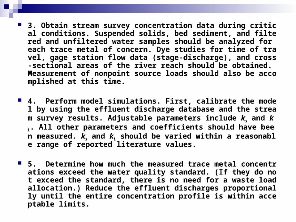
3. Obtain stream survey concentration data during critical conditions. Suspended solids, bed sediment, and filtered and unfiltered water samples should be analyzed for each trace metal of concern. Dye studies for time of travel, gage station flow data (stage-discharge), and cross-sectional areas of the river reach should be obtained. Measurement of nonpoint source loads should also be accomplished at this time.

4. Perform model simulations. First, calibrate the model by using the effluent discharge database and the stream survey results. Adjustable parameters include ks and kL. All other parameters and coefficients should have been measured. ks and kL should be varied within a reasonable range of reported literature values.

5. Determine how much the measured trace metal concentrations exceed the water quality standard. (If they do not exceed the standard, there is no need for a waste load allocation.) Reduce the effluent discharges proportionally until the entire concentration profile is within acceptable limits.

Figure 8.4 Waste load allocation for copper in the Deep River, North Carolina. Total dissolved copper concentrations in field samples and model simulation are shown. The water quality standard is 20 µg L-1.

5.3 COMPLFX FORMATION AND SOLUBILITY

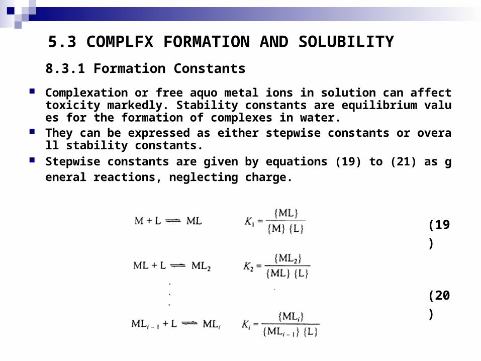
8.3.1 Formation Constants Complexation or free aquo metal ions in solution can affect toxicity marke

dly. Stability constants are equilibrium values for the formation of complexes in water.

They can be expressed as either stepwise constants or overall stability constants.

Stepwise constants are given by equations (19) to (21) as general reactions, neglecting charge.

(19)

(20)

(21)

Overall stability constants are reactions written in terms of the free aquo metal ion as reactant:

(22)

(23)

The product of the stepwise formation constants gives the overall stability constant:

(24)

For polynuclear complexes, the overall stability constant is used, and it

reflects the composition of the complex in its subscript. An example would be Fe2(OH)2

4+

(25)

(26)

Table 8.3 Logarithm of Overall Stability Constants for Formation of Complexes and Solid from Metals and Ligands at 25 °C and I = 0.0 M

Table 8.3 (Continued)

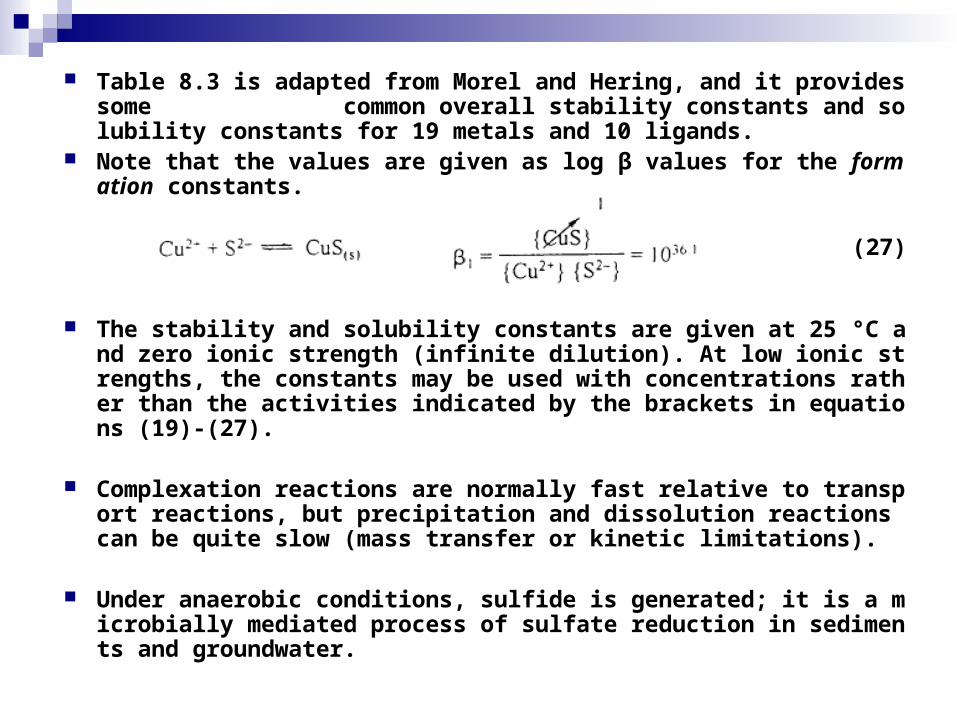
Table 8.3 is adapted from Morel and Hering, and it provides some common overall stability constants and solubility constants for 19 metals and 10 ligands.

Note that the values are given as log β values for the formation constants.

(27)

The stability and solubility constants are given at 25 °C and zero ionic strength (infinite dilution). At low ionic strengths, the constants may be used with concentrations rather than the activities indicated by the brackets in equations (19)-(27).

Complexation reactions are normally fast relative to transport reactions, but precipitation and dissolution reactions can be quite slow (mass transfer or kinetic limitations).

Under anaerobic conditions, sulfide is generated; it is a microbially mediated process of sulfate reduction in sediments and groundwater.

8.3.2 Complexation by Humic Substances

Humic substances comprise most naturally occurring organic matter (NOM) in soils, surface waters, and groundwater. They are the decomposition products of plant tissue by microbes. Humic substances are separated from a water sample by adjusting the pH to 2.0 and capturing the humic materials on an XAD-8 resin; subsequent elution in dilute NaOH is used to recover the humic substances from the resin.

In nature, soils are leached by precipitation, and runoff carries a certain amount of humic and fulvic compounds into the water.

(28) The term fulvic acids (FA) refers to a mixture of natural organics with MW ≈

200-5000, the fraction that is soluble in acid at pH 2 and also soluble in alcohol. The median molecular weight of FA is ~500 Daltons.

The fulvic fraction (FF) includes carbohydrates, fulvic acids, and polysaccharides.

(29)

Table 8.4 is a summary of metal-fulvic acid (M-FA) complexation constants.

One approach is to use conditional stability constants (such as Table 8.4) for the natural water that is being modeled

(30)

where cK is the conditional stability constant at a specified pH, ionic strength, and chemical composition. One does not always know the stoichiometry of the reaction in natural waters, whether 1:1 complexes or 1:2 complexes (M/FA) are formed, for example.

Equation (30) is simply a lumped-parameter conditional stability constant, but it does allow intercomparisons of the relative importance of complexation among different metal ions and DOC at specified conditions.

The conditional complexation constant (stability constant) should be measured for each site. Total dissolved concentrations of metals (including M-FA) are measured using atomic absorption spectroscopy or inductively coupled plasma emission spectroscopy, and the aquo free metal ion is measured by ISEs or ASV.

Table 8.4 Freshwater conditional stability constants for formation of M-FA complexes (roughly in order of binding strength)

Conditional stability constants for metal-fulvic acid complexes vary in natural waters because:

There are a range of affinities for metal ions and protons in natural organic matter resulting in a range of stability constants and acidity constants.

Conformational changes and changes in binding strength of M-FA complexes in natural organic matter result from electrostatic charges (ionic strength), differential and competitive cation binding, and, most of all, pH variations in water.

The stability constants given in Table 8.5 vary markedly with pH.

The total number of metal-titrateable groups is in the range of 0.1 - 5 meq per gram of carbon, DOC complexation capacity. Complexation of metals fulvic acid is most significant for those ions that are appreciably complexed with CO3

2- and OH- (functional groups like those contained in fulvic acid that contains carboxylic acids and catechol with adjacent - OH sites). These include mercury, copper, and lead.

Table 8.5 Fitting parameters for Five-Site Model

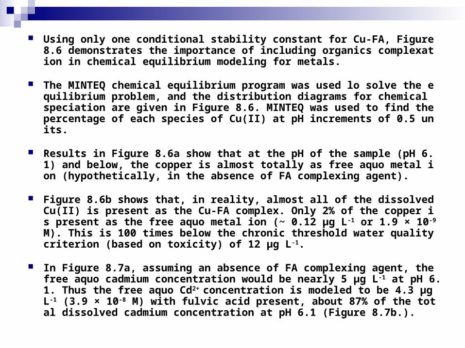
Using only one conditional stability constant for Cu-FA, Figure 8.6 demonstrates the importance of including organics complexation in chemical equilibrium modeling for metals.

The MINTEQ chemical equilibrium program was used lo solve the equilibrium problem, and the distribution diagrams for chemical speciation are given in Figure 8.6. MINTEQ was used to find the percentage of each species of Cu(II) at pH increments of 0.5 units.

Results in Figure 8.6a show that at the pH of the sample (pH 6.1) and below, the copper is almost totally as free aquo metal ion (hypothetically, in the absence of FA complexing agent).

Figure 8.6b shows that, in reality, almost all of the dissolved Cu(II) is present as the Cu-FA complex. Only 2% of the copper is present as the free aquo metal ion (~ 0.12 µg L-1 or 1.9 × 10-9 M). This is 100 times below the chronic threshold water quality criterion (based on toxicity) of 12 µg L-1.

In Figure 8.7a, assuming an absence of FA complexing agent, the free aquo cadmium concentration would be nearly 5 µg L-1 at pH 6.1. Thus the free aquo Cd2+ concentration is modeled to be 4.3 µg L-1 (3.9 × 10-8 M) with fulvic acid present, about 87% of the total dissolved cadmium concentration at pH 6.1 (Figure 8.7b.).

Figure 8.6 (a) Equilibrium chemical speciation of Cu(II) in Filson Creek, Minnesot

a, without consideration of complexation by dissolved organic carbon (fulvic acid).

(b) Equilibrium chemical speciation of Cu(II) in Filson Creek, Minnesota, with copper-fulvic acid formation constant of log K = 6.2.

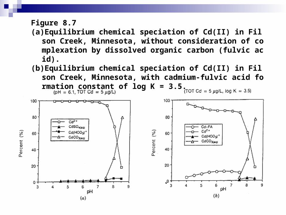
Figure 8.7 (a) Equilibrium chemical speciation of Cd(II) in Filson Creek, Minnesot

a, without consideration of complexation by dissolved organic carbon (fulvic acid).

(b) Equilibrium chemical speciation of Cd(II) in Filson Creek, Minnesota, with cadmium-fulvic acid formation constant of log K = 3.5.

Example 8.2 Lead Chemical Speciation

A chemical equilibrium program with a built-in database can be used to model the chemical speciation for Pb in natural waters. Lake Hilderbrand, Wisconsin, is a small seepage lake in northern Wisconsin with some drainage from a bog. It receives acid deposition from air emissions in the Midwest, and its chemistry reflects acid precipitation, weathering/ion exchange with sediments, heavy metals deposition, and fulvic acids.

It was probably never an alkaline lake because much of its water comes directly onto the surface of the lake via precipitation and from drainage or bogs; the current pH is 5.38. It has 12.0 units of color (Pt-Co wits), an we can assume a FA concentration of 2.9 × 10-5 M. The log cK for Pb-FA in the system is in the range of 4-5.

Use a chemical equilibrium model such as MINTEQA2 to solve for all the Pb species in solution from pH 4 to 8 with increments of 0.5 units. The temperature of the sample was 13.7 °C.

Its ion chemistry (in mg L-1) was the following: Ca+2 = 1.37, Na+ = 0.21, Mg2+ = 0.31, K+ = 0.64, ANC (titration alkalinity as CaC03) = 0.03, SO4

2- = 5.25, Cl- = 0.38, Cd(II) = 0.000037, and Pb(II) = 0.00035 mg L-1. Is the Pb(II) expected to be present as the free aquo metal ion?

Solution: All the ions must be converted to mol L-1 concentration units. The ion balance should be checked; the sum of the cations minus the anions should be within 5% of the sum of the anions. At pH 5.38 some of the FA is anionic (fulvate), so it might need to be included as an anion in the charge balance. In this case, there is a good charge balance so the fulvic acid either

(1) has an acidity constant near the pH of the solution and it does not contribute much to the charge, and/or

(2) a portion of the Ca2+ is actually complexed by FA-, which fortuitously causes the calculated ∑(+) charges to be nearly equal to the ∑(-) charges.

The ion balance checks to within 2.4%.

At high pH we expect PbC03(aq) and PbOH+; at low pH we expect Pb2+ and possibly Pb-FA.

The acidity constant for HFA is log K = -4.8. We neglect the complex of PbSO4

0 because the stability constant is rather small (Table 8.3). As we increase pH from 4 to 8, we can assume an open or a closed system with respect to CO2(g). In this case, a closed system was assumed.

Results for three different cases are given in Figure 8.8. The model is quite sensitive to the log cK that is assumed for the Pb-FA complex. Given a log c

K = 5.0, most of the total lead that is present in solution is complexed with fulvic acid at pH 5.38.

Schnitzer and Skinner suggest an even stronger Pb-FA complex at pH 5 with log cK = 6.13 in soil water. Most of the Pb(II) is apparently complexed with fulvate at pH 5.38 in Lake Hilderbrand. It is not considered toxic; the chronic water quality criterion for fresh water is 3.2 µg L-1.

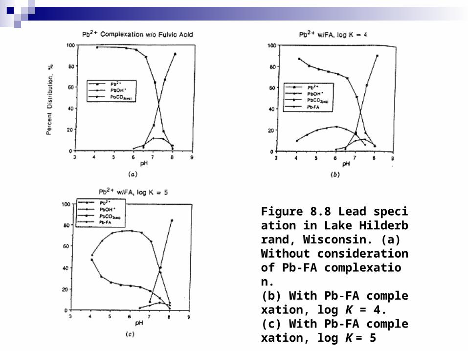
Figure 8.8 Lead speciation in Lake Hilderbrand, Wisconsin. (a) Without consideration of Pb-FA complexation. (b) With Pb-FA complexation, log K = 4. (c) With Pb-FA complexation, log K = 5

Example 8.2 brings up an important model limitation or fulvic acid binding for metal ions in natural waters. It is not clear how much competition exists among divalent cations. For example, the reaction between Ca-FA and Pb2+ in solution is certainly less favorable thermodynamically than FA with Pb2+.

These competition reactions (ligand exchange) are generally not considered in chemical equilibrium modeling.

(31)

The log cK for Al-FA is approximately 5.0 (quite a strong complex), and this competition was not considered in Example 8.2. Also, the affinity of Fe(III) for FA is almost equal to that of Pb-FA.

Figure 8.9 shows the nature of those binding sites where adjacent carboxylic acid and phenolic groups are hydrogen bonded to form a polymeric structure with considerable stability.

Figure 8.9 Typical structure of dissolved organic matter in natural waters with hydrogen bonding and bridging among functional groups that also make binding sites for metals.

8.4 SURFACE COMPLEXATION/ADSORPTION

8.4.1 Particle-Metal Interactions

In addition to aqueous phase complexation by inorganic and organic ligands, meta1 ions can form surface complexes with particles in natural waters. This phenomenon is variously named in scientific literature as surface complexation ion exchange, adsorption, metal-particle binding, and metals scavenging by particles.

Particles in natural water are many and varied, including hydrous oxides, clay particles, organic detritus, and microorganisms. They range a wide gamut of sizes (Figure 8.10).

Particles provide surfaces for complexation of metal ions, acid-base reactions, and anion sorption.

where SOH represents hydrous oxide surface sites, M2+ is the metal ion, and A2-

is the anion.

(32)

(33)

(34)

(35)

(36)

(37)

(38)

Figure 8.10 Particle size spectrum in natural waters

Figure 8.11 shows the "sorption edges" for three hypothetical metal cations forming surface complexes on hydrous oxides (e.g., amorphous iron oxides FeOOH(s) or aluminum hydroxide Al(OH)3(s)). Equations (32) and (33) indicate that the higher is the pH of the solution, the greater the reactions will proceed to the right.

The adsorption edge culminates in nearly 100% of the metal ion bound to the surface of the particles at high pH. At exactly what pH that occurs depends on the acidity and basicity constants for the surface sites, equations (34) and (35), and the strength of the surface complexation reaction, equations (32) and (33).

Anions can form surface complexes on hydrous oxides (Figure 8.11). Most particles in natural waters are negatively charged at neutral pH. At low pH, the surfaces become positively charged and anion adsorption is facilitated equations (37) and (38). Weak acids (such as organic acids, fulvic acids) typically have a maximum sorption near the pH of their first acidity constant (pH = pKa), a consequence of the equilibrium equations (34)-(36).

Figure 8.11 Surface complexation and sorption edges for metal cations and organic anions onto hydrous oxide surface

In Figure 8.12, sorption edges for surface complexation of various metals on hydrous ferric oxide (HFO) are depicted.

Metal ions on the left of the diagram form the strongest surface complexes (most stable) and those on the right at high pH form the weakest.

Figure 8.12 Extent of surface complex formation as a function of pH (measured as mol % of the metal ions in the system adsorbed or sur-face bound). [TOT Fe] = 10-3 M (2 × 10-4 mol reactive sites L-1): metal concentrations in solution = 5 × 10-7 M; I = 0.1 M NaN03.

8.4.2 Natural Waters

Particles from lakes and rivers exert control on the total concentration or trace metals in the water column. The adsorption-sedimentation process scavenges metals from water and carries them to the sediments.

Muller and Sigg showed that particles in the Glatt River, Switzerland, adsorbed more than 30% of Pb(II) in whole water samples (Figure 8.14).

lt is interesting that small quantities of chelates in natural waters and groundwater can exert a significant influence on trace metal speciation. At concentrations typically measured in rivers receiving municipal wastewater discharges, chelation of Pb(II) accounts for more than half of dissolved lead (Figure 8.14).

They form stable chelate complexes (with multidentate ligands) on trace metal ions, rendering them mobile and nonreactive. In natural waters, chelates such as EDTA are biodegraded or photolyzed slowly, and steady-state concentrations can be sufficient to affect trace metal speciation.

Figure 8.14

Speciation of Pb(II) in the Glatt River, Switzerland, including (a) adsorption onto particulates and (b) comple-xation by EDTA and NTA chelates, which are measured in the environment.

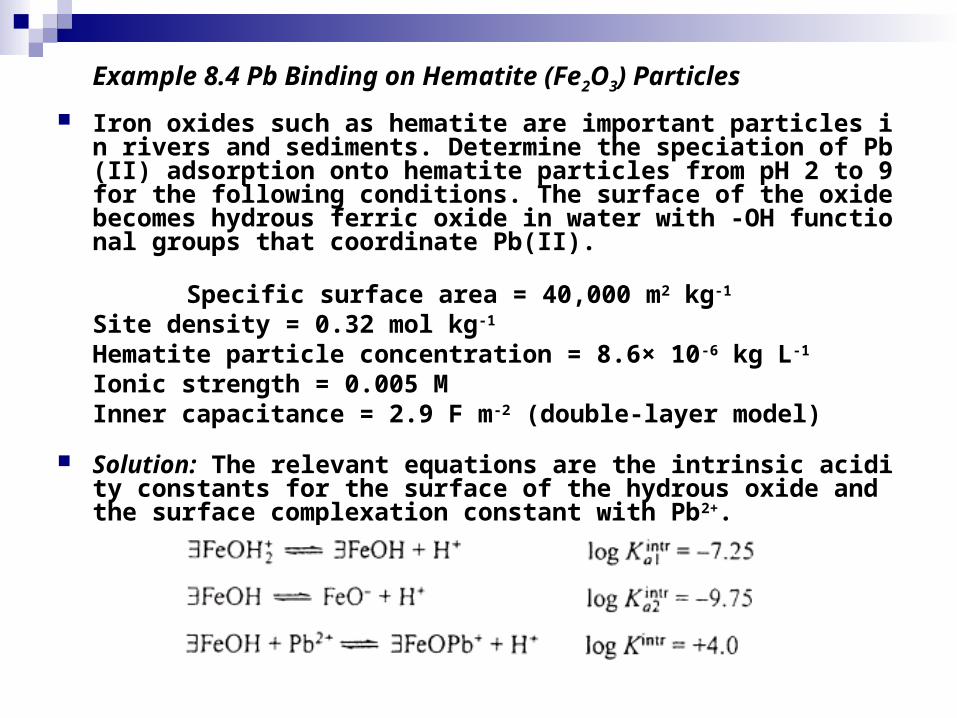
Example 8.4 Pb Binding on Hematite (Fe2O3) Particles

Iron oxides such as hematite are important particles in rivers and sediments. Determine the speciation of Pb(II) adsorption onto hematite particles from pH 2 to 9 for the following conditions. The surface of the oxide becomes hydrous ferric oxide in water with -OH functional groups that coordinate Pb(II).

Specific surface area = 40,000 m2 kg-1

Site density = 0.32 mol kg-1

Hematite particle concentration = 8.6× 10-6 kg L-1

Ionic strength = 0.005 MInner capacitance = 2.9 F m-2 (double-layer model)

Solution: The relevant equations are the intrinsic acidity constants for the surface of the hydrous oxide and the surface complexation constant with Pb2+.

Recall that the electrostatic effect of bringing a Pb2+ atom to the surface of the oxide must be considered (the coulombic correction factor).

This is accounted for in the program by correcting the intrinsic surface equilibrium constants.

The column in the matrix below, "surface charge" refers to the coulombic corr

ection factor exp(-Fψ/RT), which multiplies the intrinsic equilibrium constant to obtain the apparent equilibrium constant in the Newton-Raphson solution.

The total concentration of binding sites for the mass balance is the product of the site density and the hematite particle concentration, 2.75 × 10-6 M.

The matrix can be used to solve the problem using a chemical equilibrium program. Results are shown in Figure 8.15. Interactive models such as MacµQL will prompt the user to provide information about the adsorption model (double-layer model in this case) and the inner capacitance.

Note how sharp the "sorption edge" is in Figure 8.15 between pH 4 and 6. Above pH 6, almost all of the Pb(Il) is adsorbed under these conditions. Lines in the pC versus pH plot of Figure 8.15 are "wavy“ due to the coulombic correction factor.

Following are a few types of particles suspended in natural waters and their surface groups.

Clays (-OH groups and H+ exchange). CaCO3 (carbonato complexes and coprecipitation). Algae + bacteria (binding and active transport for Cu, Zn, Cd, AsO4

3-, ion change).

FeOOH (oxygen donor atoms, high specific surface area).

MnO2 (oxygen donor atoms, high specific surface area). Organic detritus (phenolic and carboxylic groups). Quartz (oxide surface with coatings).

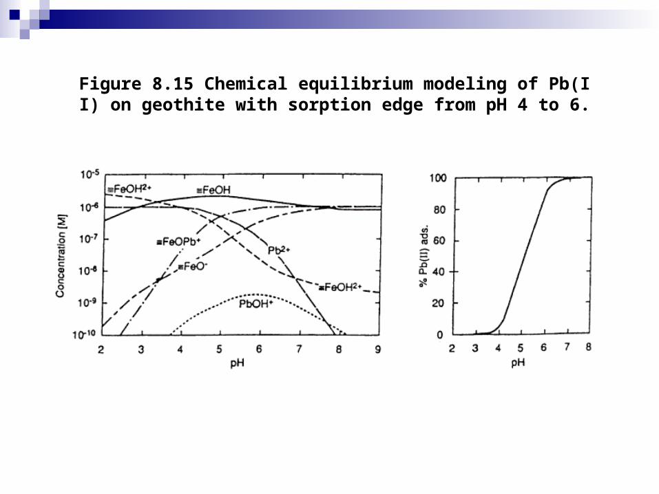
Figure 8.15 Chemical equilibrium modeling of Pb(II) on geothite with sorption edge from pH 4 to 6.

8.4.3 Mercury as an Adsorbate

One of the most difficult metals to model is Hg(II) because it undergoes many complexation reactions, both in solution and at the particle surface, and it is active in redox reactions as well.

Hg(II) forms strong complexes with Cl- in seawater, OH-, and organic ligands in fresh water. On surfaces, it seeks to coordinate with oxygen donor atoms in inner-sphere complexes.

Tiffreau et al. have used the diffuse double-layer model with two binding sites to describe the adsorption of Hg(II) onto quartz (α-SiO2) and hydrous ferric oxide in the laboratory over a wide range of conditions.

It was necessary to invoke ternary complexes, that is, the complexation of three species together, in this case SOH, Hg2+, and Cl-. The HFO was prepared in the laboratory, 89 g mol-1 Fe (298.15 K, I = 0 M).

Surface area = 600 m2 g-1

Site density1 = 0.205 mol mol-1 Fe (weak binding sites) Site density2 = 0.029 mol mol-1 Fe (strong binding sites) Acidity constant1 FeOOH2

+ pKa1intr = 7.29

Acidity constant2 FeOOH pKa2intr = 8.93

Quartz grains have a much lower surface area and are generally less important for sorption in natural waters.

Surface area = 4.15 m2 g-1

Site density = 4.5 sites nm-2

Acidity constant1 SiOH2+ pKa1

intr = -0.95 Acidity constant2 SiOH pKa2

intr = 6.95 Solids concentration = 40 g L-1 SiO2

Figure 8.16: results of the simulation for adsorption (Hg(II)T = 0.184 µM) onto quartz at I = 0.1 M NaClO4. Equilibrium constants for the surface complexation reactions are given in Table 8.6.

Figure 8.16 shows that metal sorption can be "amphoteric“ just like metal oxides and hydroxides. The pH of zero charge for the quartz is pH ~3. As the surface becomes more negatively charged above pH 3, the sorption edge for Hg(II) on α-SiO2 is observed.

Even in pure laboratory systems, modeling the sorption of trace metals on particles becomes complicated. That is why many investigators use a conditional equilibrium constant approach, that or the solids/water distribution coefficient, Kd.

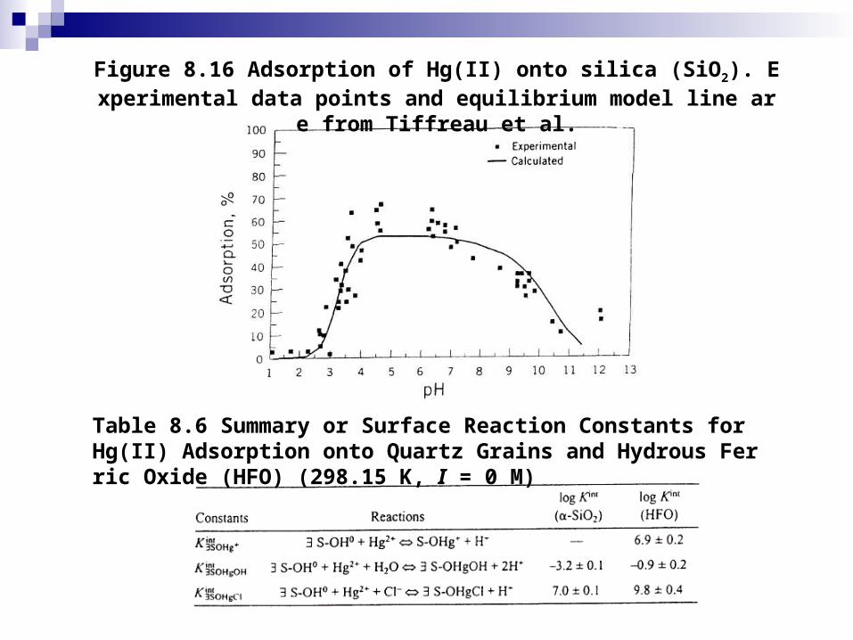
Figure 8.16 Adsorption of Hg(II) onto silica (SiO2). Experimental data points and equilibrium model line are from Tiffreau et al.

Table 8.6 Summary or Surface Reaction Constants for Hg(II) Adsorption onto Quartz Grains and Hydrous Ferric Oxide (HFO) (298.15 K, I = 0 M)

8.5 STEADY-STATE MODEL FOR METALS IN LAKES

8.5.1 Introduction Surface coordination of metals with particles in lakes may be described in

the simplest case as(39)

(40)

Traditionally, researchers have described metals adsorption in natural waters with an empirical distribution coefficient defined as the ratio or the adsorbed metal concentration to the dissolved metal fraction. For the case described by equation (39), the distribution coefficient would be defined as the following:

(41) where [SOM+]/[SOH) is expressed in µg kg-1 solids and M2+ is in µg L-1. By combining equations (40) and (41), we see that Kd is inversely proportional t

o the H+ ion concentration. (42)

Kd is expressed in units of µg kg-1 adsorbed metal ion per µg L-1 dissolved meta

l ion (L kg-1).

8.5.2 Steady-State Model

We can formulate a simple steady-state mass balance model to describe the input of metals to a lake.

(43) where V = lake volume, L3

CT = total (unfiltered) metal concentration suspended in the lake, ML-3

I = precipitation rate, LT-1

CT precip = total metal concentration in precipitation, ML-3

A = surface area of the lake, L2

CT air = metal concentration in air, ML-3 Vd = dry deposition velocity, LT- 1

ks = sedimentation rate constant, T-1

Q = outflow discharge rate, L3T-1

fp = particulate fraction of total metal concentration in lake, dimensionless = KdM/(1 + KdM)

M = suspended solids in the lake, ML-3

Kd = solids/water distribution coefficient, L3M-1

Under steady-state conditions, equation (43) can be solved for the average total metals concentration (unfiltered) in the lake.

(44)

where τ = mean hydraulic detention time of the lake = V/Q, T H = mean depth of the lake, L

or (45)

where CT in = total input concentration or wet plus dry deposition, ML-3

= (Iτ CT precip + vdτ CT air)/H

From equation (45), one can estimate the fraction of metal removed by the lake due to sedimentation.

(46) Equation (46) can be used to estimate the "trap efficiency" of the lake for

metals. The dimensionless number KdM is involved in equation (46) through the particulate adsorbed fraction of metal, fp = KdM/(1 + KdM).

Figure 8.17 shows that the fraction of metal that is removed from the lake by sedimentation increases with KdM and ksτ. Lakes with very short hydraulic detention times, τ, are not able to remove all of the adsorbed metal by sedimentation even if the KdM parameter is very large because the residence time is not long enough.

Model equation (46) provides a steady-state estimate of the fraction of metals that are adsorbed and sedimented to the bottom or the lake. To use the model, we must know the following parameters: ks, τ, Kd, and the suspended solids M (Table 8.7).

Values for Kd vary considerably from lake to lake because the nature or particles differs and aqueous phase complexing agents may vary.

Kd values decrease with increasing concentration of total suspended solids according to empirical relationships.

Figure 8.17 Effect of two dimensionless numbers on the fraction of metal inputs that are removed by sedimentation in lakes. KdM is the distribution coefficient times the suspended solids concentration. ksτ is the sedimentation rate constant times the mean hydraulic detention time Theoretical curves are basedon a simple mode1 with completely mixed reactor assumption under steady-stale conditions.

Table 8.7 Parameters in Steady-State Model [eq`n (46)]

Example 8.5 Steady-State Model for Pb in Lake Cristallina

Lake Cristallina is a small, oligotrophic lake at 2400 m above sea level in the southern Alps of Switzerland. It has a mean hydraulic detention time of only 10 days, a particle settling velocity of 0.1 m d-1, a mean depth of 1 m, and a Kd value of 105 L kg-1 for Pb at pH 6. The suspended solids concentration is 1 mg L-1. Estimate the fraction of Pb(II) that is adsorbed to suspended particles and the fraction that is sedimented. Hypothetically, what would be the variation in the results if the pH or the lake varied between pH 5 and 8, but other parameters remained constant?

Solution: We can calculate two dimensionless parameters ksτ and KdM and esti

mate the fraction in the particulate adsorbed phase, fp, and the fraction removed to the sediment [equation (46)]. At pH 6,

Assuming a linear dependence of Kd on 1/[H+] as indicated by equation (42), one can complete the calculations for pH 5, 7, and 8. Results are plotted in Figure 8.18. In reality, the relationship between Kd and [H+] is complicated by the stoichiometry of surface complexation and aqueous phase complexing ligands. The best way to establish the effect of pH on Kd is experimentally at each location.

Figure 8.18 shows a steep sorption edge for Pb in Lake Cristallina as pH increases. Because Lake Crystallina has such a short hydraulic detention time, little of the Pb(ll) is removed at pH 5-6. Thus acidic lakes have significantly higher concentrations of toxic metals because less is removed by particle adsorption and sedimentation.

Also, when the pH is low, there is a greater fraction of the total Pb(II) that is present as the free aquo metal ion (more toxicity). Table 8.8 is a compilation of some European lakes and trace metal concentrations relative to Lake Cristallina.

The pH dependence of trace metal binding on particles affects a number of acid lakes receiving atmospheric deposition. Lower pH waters have significantly higher concentrations of zinc, for example (Figure 8.19).

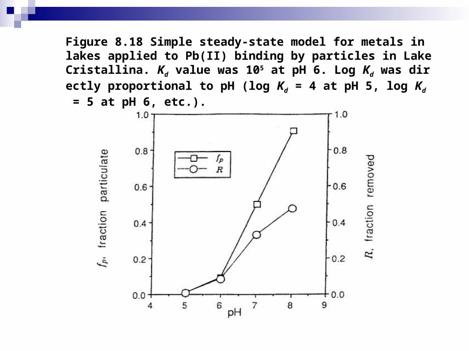
Figure 8.18 Simple steady-state model for metals in lakes applied to Pb(II) binding by particles in Lake Cristallina. Kd value was 105 at pH 6. Log Kd was directly proportional to pH (log Kd = 4 at pH 5, log Kd = 5 at pH 6, etc.).

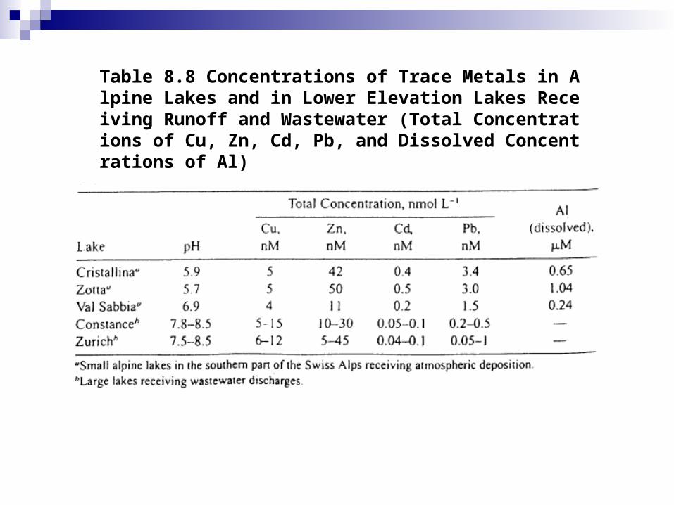
Table 8.8 Concentrations of Trace Metals in Alpine Lakes and in Lower Elevation Lakes Receiving Runoff and Wastewater (Total Concentrations of Cu, Zn, Cd, Pb, and Dissolved Concentrations of Al)

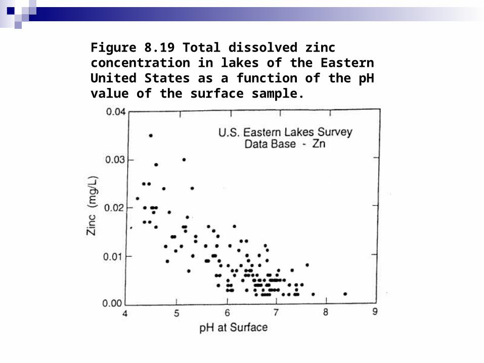
Figure 8.19 Total dissolved zinc concentration in lakes of the Eastern United States as a function of the pH value of the surface sample.

Solubility exerts some control on metals particularly under anaerobic conditions of sediments. And particles can scavenge trace metals, decreasing the total dissolved concentration remaining in the water column. We have seen that for Pb(II) both surface complexation on particles and aqueous phase complexation are important.

For Cu(II), organic complexing agents are important, especially algal exudates and organic macromolecules.

The modeler must be aware of factors affecting chemical speciation in natural waters, particularly when toxicity is the biological effect under investigation. The controls on trace metals are threefold:

Particle scavenging (adsorption). Aqueous phase complexation. Solubility.

They all can be important under different circumstances and the relative importance of each can be modeled. The first process, particle scavenging, is affected by the aggregation of particles in natural waters.

8.5.3 Aggregation, Coagulation, and Flocculation

Coagulation in natural waters refers to the aggregation or particles due to electrolytes. The classic example is coagulation of suspended solids as salinity increases toward the mouth of an estuary. Polymers are also known to "bridge" particles causing flocculation.

Organic macromolecules may be effective in aggregating particles in natural waters, especially near the sediment-water interface where particle concentrations are high.

Particles less than 1.0 µm are usually considered to be in colloidal form, and they may be suspended for a long time in natural waters because their gravitational settling velocities are less than 1 m d-1.

Colloidal suspensions are “stable”, and they do not readily settle or aggregate in solution. Fine particles are usually negatively charged at neutral pH [with the exception of calcite, aluminum oxide, and other nonhydrated (crystalline) metal oxides].

Algae, bacteria, and biocolloids are negatively charged and emit organic macromolecules (e.g., polysaccharides) that may serve to stabilize the colloidal suspension and to disperse particles in the solution.

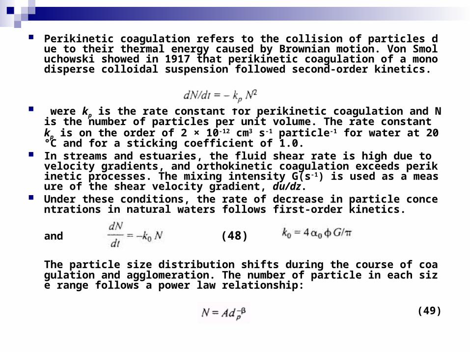
Perikinetic coagulation refers to the collision of particles due to their thermal energy caused by Brownian motion. Von Smoluchowski showed in 1917 that perikinetic coagulation of a monodisperse colloidal suspension followed second-order kinetics.

(47)

were kp is the rate constant for perikinetic coagulation and N is the number of

particles per unit volume. The rate constant kp is on the order of 2 × 10-12 cm3 s-

1 particle-1 for water at 20 °C and for a sticking coefficient of 1.0. In streams and estuaries, the fluid shear rate is high due to velocity gradients,

and orthokinetic coagulation exceeds perikinetic processes. The mixing intensity G(s-1) is used as a measure of the shear velocity gradient, du/dz.

Under these conditions, the rate of decrease in particle concentrations in natural waters follows first-order kinetics.

and (48)

The particle size distribution shifts during the course of coagulation and agglomeration. The number of particle in each size range follows a power law relationship:

(49)

8.6 REDOX REACTIONS AND TRAGE METALS

8.6.1 Mercury and Redox Reactions

Mercury has valence states of +2, +1, and 0 in natural waters. In anaerobic sediments, the solubility product or HgS is so low that Hg(II)(aq) is below detection limits, but in aerobic waters a variety of redox states and chemical transformations are of environmental significance.

Mercury is toxic to aquatic biota as well as humans. In humans, it binds sulfur groups in recycling amino acids and enzymes, rendering them inactive.

Mercury is released into air by outgassing of soil, by transpiration and decay of vegetation, and by anthropogenic emissions from coal combustion. Most mercury is adsorbed onto atmospheric particulate matter or in the elemental gaseous state.

Humic substances form complexes, which are adsorbed onto particles, and only a small soluble fraction of mercury is taken up by biota.

Pelagic organisms agglomerate and excrete the mercury-bearing clay panicles, thus promoting sedimentation as one sink of mercury from the midoceanic food chain. Another source of mercury to biota is uptake of dissolved mercury by phytoplankton and algae.

Figure 8.20 shows the inorganic equilibrium Eh-pH stability diagram for Hg in fresh water and groundwater. Mercury exists primarily as the hydroxy complex Hg(OH)2

0 in aqueous form in surface waters.

At chemical equilibrium in soil water and groundwater, inorganic mercury is converted to Hg(ag)

0, although the process may occur slowly.

A purely inorganic chemical equilibrium model should consider the many hydroxide and chloride complexes of mercury given by Table 8.9 The chloro complexes are important in seawater.

It is apparent that most mercury compounds released into the environment can be directly or indirectly transformed into monomethylmercury cation or dimethylmercury via bacterial methylation. At low mercury contamination levels, dimethylmercury is the ultimate product of the methy1 transfer reactions, whereas if higher concentrations of mercury are introduced, monomethylmercury is predominant.

If the lakes are acid, mercury is methylated to CH3Hg+ and biocomcentrated by fish. The greater is the organic matter content of sediments, the greater is the tendency for methylation (formation of CH3Hg+) and bioconcentration by fish.

Figure 8.20 Stability fields for aqueous mercury species at various Eh and pH values (chloride and sulfur concentrations of 1 mM each were used in the calculation; common Eh-pH ranges for groundwaterare also shown).

Figure 8.21: kinetics control the bacterial methylation, demethylation, and bioconcentration of mercury in the aquatic environment. Thus an equilibrium approach such as that given by Table 8.9 is not sufficient.

We must couple chemical equilibrium expressions with mass balance kinetic equations and solve simultaneously in order to model such problems.

As a first approach to the problem, let us assume that most of the processes depicted in Figure 8.21 can be modeled using first-order reaction kinetics. Rate constants are conditional and site specific because they depend on environmental variables such as organic matter content of sediments, pH, and fulvic acid concentration.

We can neglect the disproportionation reaction:

(50)

Also, the formation of dimethyl mercuric sulfide (CH3S-HgCH3) is known to be important in marine environments, but it is neglected here.

Figure 8.21 Schematic of Hg(II) reactions in a lake including bioaccumulation, adsorption, precipitation, methylation, and redox reactions

Table 8.9 Stability Constants Used in the Inorganic Complexation Model for Hg(II),298.15 K, I = 0 M

A chemical equilibrium submodel would be used to estimate the fraction of total Hg(II) that was adsorbed onto hydrous oxides and particulate organic matter, [Hg2+]ads. It would also calculate the amount of Hg(Il) that precipitates as HgS(s).

The mass balance model is used to calculate the kinetics of redox reactions among the species Hg2+, Hg0, CH3Hg+, and (CH3)2Hg0, as well as the rate of nonredox processes such as uptake by fish, volatilization to the atmosphere, and sedimentition of particulate-adsorped mercury and precipitated solids (if any).

Simplified mass balance equations for a batch system (such as a lake) are given eq`ns (51)-(54):

(51)

(52)

(53)

(54)

(55)

where [Hg(II)]T = total Hg(II) concentration (dissolved and particulate), ML-3

t = time, T Fd2 = total inputs including wet and dry deposition of Hg(II),

ML-2T-1

Fdo = total inputs of Hg0, ML-2T-1

H = mean depth of the lake, L kox = oxidation rate constant for Hg0 →_Hg(II), T-1

[Hg0] = dissolved elemental mercury concentration, ML-3

τ = mean hydraulic detention time, T km = methylation rate constant, L3 cells-1 T-1

[Hg(II)] = Hg(II) aqueous concentration, ML-3

[Bacteria] = methylating bacteria concentration, cells L-1

kFA = rate constant for reduction of Hg(Il), L-3 mol-1T-1

[FA] = fulvic acid (DOC) concentration, mol L-3 kdi = rate constant for chemical dimethylation, T-1

[Hg(II)]ads = adsorbed Hg(II) concentration on particles, ML-3

ks1 = sedimentation rate constant of adsorbed Hg(II), T-1

ks2 = sedimentation rate constant of precipitated HgS, T-1

ks3 = sedimentation rate constant for metallic mercury, T-1

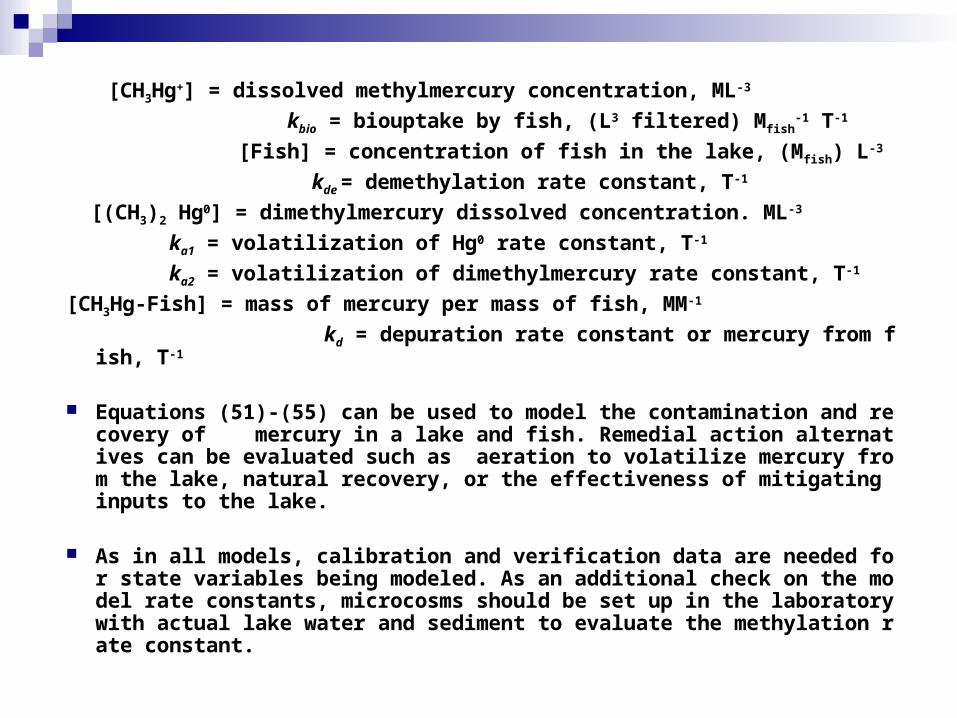
[CH3Hg+] = dissolved methylmercury concentration, ML-3

kbio = biouptake by fish, (L3 filtered) Mfish-1 T-1

[Fish] = concentration of fish in the lake, (Mfish) L-3

kde = demethylation rate constant, T-1

[(CH3)2 Hg0] = dimethylmercury dissolved concentration. ML-3

ka1 = volatilization of Hg0 rate constant, T-1

ka2 = volatilization of dimethylmercury rate constant, T-1

[CH3Hg-Fish] = mass of mercury per mass of fish, MM-1

kd = depuration rate constant or mercury from fish, T-1

Equations (51)-(55) can be used to model the contamination and recovery o

f mercury in a lake and fish. Remedial action alternatives can be evaluated such as aeration to volatilize mercury from the lake, natural recovery, or the effectiveness of mitigating inputs to the lake.

As in all models, calibration and verification data are needed for state variables being modeled. As an additional check on the model rate constants, microcosms should be set up in the laboratory with actual lake water and sediment to evaluate the methylation rate constant.

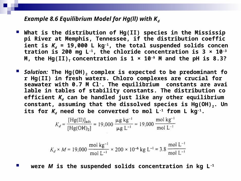
Example 8.6 Equilibrium Model for Hg(ll) with Kd

What is the distribution of Hg(II) species in the Mississippi River at Memphis, Tennessee, if the distribution coefficient is Kd = 19,000 L kg-1, the total suspended solids concentration is 200 mg L-1, the chloride concentration is 3 × 10-3 M, the Hg(II)T concentration is 1 × 10-9 M and the pH is 8.3?

Solution: The Hg(OH)2 complex is expected to be predominant for Hg(II) in fresh waters. Chloro complexes are crucial for seawater with 0.7 M Cl-. The equilibrium constants are available in tables of stability constants. The distribution coefficient Kd can be handled just like any other equilibrium constant, assuming that the dissolved species is Hg(OH)2. Units for Kd need to be converted to mol L-1 from L kg-1.

were M is the suspended solids concentration in kg L-1

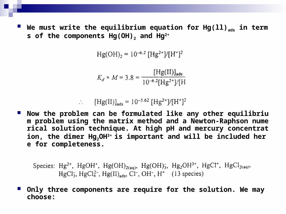
We must write the equilibrium equation for Hg(ll)ads in terms of the components Hg(OH)2 and Hg2+

Now the problem can be formulated like any other equilibrium problem us

ing the matrix method and a Newton-Raphson numerical solution technique. At high pH and mercury concentration, the dimer Hg2OH3+ is important and will be included here for completeness.

Only three components are require for the solution. We may choose:

Components: Hg2+, Cl-, and H+ (3 components)

Results of the calculation show that 79% of the Hg(ll)T is adsorbed to suspe

nded solids under these conditions. The remainder is primarily as Hg(OH)

2(aq). Thus the assumption that the dissolved Hg(OH)2 species represents Hg

(II)(aq) in the distribution coefficient was valid.

Answer:

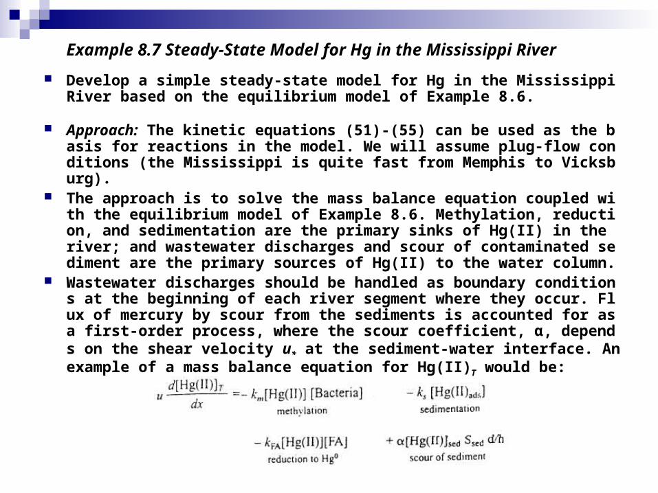
Example 8.7 Steady-State Model for Hg in the Mississippi River

Develop a simple steady-state model for Hg in the Mississippi River based on the equilibrium model of Example 8.6.

Approach: The kinetic equations (51)-(55) can be used as the basis for reactions in the model. We will assume plug-flow conditions (the Mississippi is quite fast from Memphis to Vicksburg).

The approach is to solve the mass balance equation coupled with the equilibrium model of Example 8.6. Methylation, reduction, and sedimentation are the primary sinks of Hg(II) in the river; and wastewater discharges and scour of contaminated sediment are the primary sources of Hg(II) to the water column.

Wastewater discharges should be handled as boundary conditions at the beginning of each river segment where they occur. Flux of mercury by scour from the sediments is accounted for as a first-order process, where the scour coefficient, α, depends on the shear velocity u* at the sediment-water interface. An example of a mass balance equation for Hg(II)T would be:

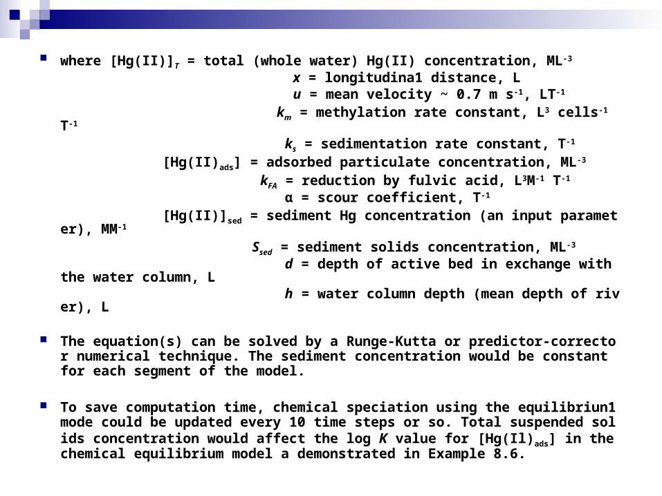
where [Hg(II)]T = total (whole water) Hg(II) concentration, ML-3

x = longitudina1 distance, L u = mean velocity ~ 0.7 m s-1, LT-1 km = methylation rate constant, L3 cells-1 T-1

ks = sedimentation rate constant, T-1

[Hg(II)ads] = adsorbed particulate concentration, ML-3

kFA = reduction by fulvic acid, L3M-1 T-1 α = scour coefficient, T-1

[Hg(II)]sed = sediment Hg concentration (an input parameter), MM-1

Ssed = sediment solids concentration, ML-3

d = depth of active bed in exchange with the water column, L h = water column depth (mean depth of river), L

The equation(s) can be solved by a Runge-Kutta or predictor-corrector numerical technique. The sediment concentration would be constant for each segment of the model.

To save computation time, chemical speciation using the equilibriun1 mode could be updated every 10 time steps or so. Total suspended solids concentration would affect the log K value for [Hg(Il)ads] in the chemical equilibrium model a demonstrated in Example 8.6.

8.6.2 Arsenic and Redox Reactions

The metalloid arsenic provides a challenge for modelers due to its redox reaction and relatively complex adsorption chemistry. It can be modeled in a manner similar to mercury even though it exists primarily as an anion in natural waters, soils, and sediments.

Arsenate, HAsO42-, is the primary anion ill aerobic surface waters, and arsenit

e (H3AsO3 or H2AsO3-) is the primary species in groundwater (Figure 8.22).

Arsenate adsorbs to iron oxides and hydroxides especially under low pH conditions when hydrous oxides have a positive surface charge. Oxidation of arsenite to arsenate by dissolved oxygen occurs slowly at neutral pH, but it can be acid or base catalyzed.

Heterogeneous oxidation of arsenite on hydrous ferric oxides is also possible. Photoreduction of arsenate to arsenite in the euphotic zone and in the presence of algae is possible.

Under extremely reducing conditions it is possible to form arsine, AsH3, with arsenic in the - 3 valence state. Arsine is very toxic to aquatic biota, but it is rare1y measured in natural waters.

More common under reducing conditions is the formation of polysulfide precipitates such as As2S3 or AsS2

- shown in Figures 8.22 and 8.23.

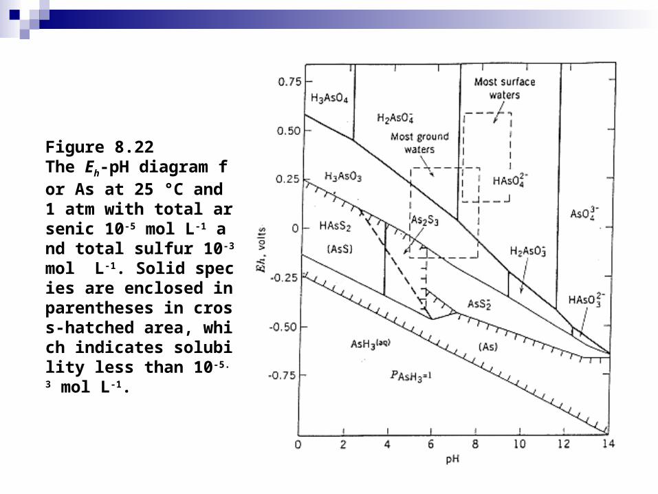
Figure 8.22 The Eh-pH diagram for As at 25 °C and 1 atm with total arsenic 10-5 mol L-1 and total sulfur 10-3 mol L-1. Solid species are enclosed in parentheses in cross-hatched area, which indicates solubility less than 10-5.3 mol L-1.

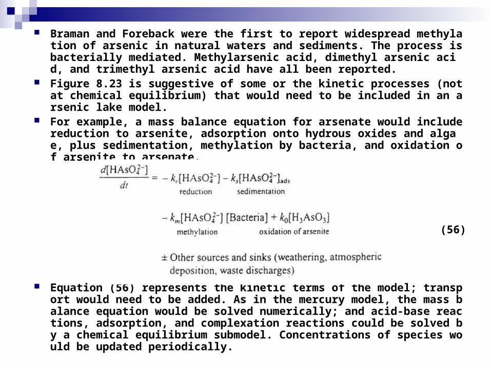
Braman and Foreback were the first to report widespread methylation of arsenic in natural waters and sediments. The process is bacterially mediated. Methylarsenic acid, dimethyl arsenic acid, and trimethyl arsenic acid have all been reported.

Figure 8.23 is suggestive of some or the kinetic processes (not at chemical equilibrium) that would need to be included in an arsenic lake model.

For example, a mass balance equation for arsenate would include reduction to arsenite, adsorption onto hydrous oxides and algae, plus sedimentation, methylation by bacteria, and oxidation of arsenite to arsenate.

(56)

Equation (56) represents the kinetic terms of the model; transport would need to be added. As in the mercury model, the mass balance equation would be solved numerically; and acid-base reactions, adsorption, and complexation reactions could be solved by a chemical equilibrium submodel. Concentrations of species would be updated periodically.

Figure 8.23 Schematic of arsenic speciation and redox reaction in a thermally stratified lake ecosystem

8.7 METALS MIGRATION IN SOILS

Trace metals with large Kd values accumulate in soils and, even after anthropogenic inputs to soils Cave been curtailed, recovery times can be lengthy. Accumulation may result from:

(1) atmospheric deposition of metals such as Cd, Hg, Pb, and Zn (Chapter);

(2) industrial discharges from landfilling, spray irrigation of wastes, mine wastes, compost, and sewage sludge applications;

(3) unintentional addition of metals to land by fertilization, such as Cd in phosphate fertilizer, or selenium and arsenic in irrigation return water. In addition, toxic metals such as Al, Zn, and Be that occur naturally in soil minerals can be liberated due to acidification of soils by acid deposition.

A transport equation for metals migration in the unsaturated zone.

(57)

No reaction terms are necessary if total dissolved metal is being modeled. When redox reactions are important and the various valence states of the metals have different Kd values, then a coupled set of equations is necessary, one equation for each valence state of relevance. The rainfall percolation rate is defined as the precipitation rate minus evapotranspiration.

Assuming a linear adsorption isotherm for low concentrations of trace metals (r = KdC), it is possible to substitute for the adsorbed concentration, r, in terms of dissolved total metal, C:

(58)

(59)

(60)

where Rf = retardation factor due to adsorption of metal, dimensionless

Kd = soil/water distribution coefficient, L3M-1 (liters kg-1)

Speciation models of trace metals in soi1s should include adsorption of metals to binding sites. Both organic and inorganic binding sites may be necessary for a general model that could be used at many different sites.

A chemical equilibrium model is given by the matrix of reactions below. There are 15 species and 7 components (including the coulombic correction factor, the dummy component recorded as surface charge). Local environmental conditions are needed for the site density of SOH (mol L-1 of soil water) and the total concentration of cadmium and ligands (v, w, x, y, and z).

The Kd for cadmium adsorption by iron oxides and aluminum oxides is defined by the equation for species 6 in Table 8.10 when free aquo metal ion is the predominant dissolved species.

(61) Rearranging:

(62)

Figure 8.24: results of column experiments with Cd-contaminated soil from an electroplating operation.

Table 8.10 Matrix of Reaction for Chemical Equilibrium Model of Cadmium in Soils

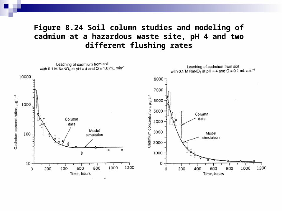
Figure 8.24 Soil column studies and modeling of cadmium at a hazardous waste site, pH 4 and two different flushing rates

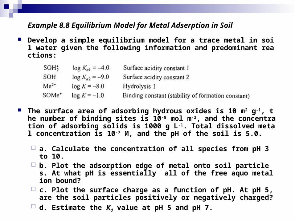
Example 8.8 Equilibrium Model for Metal Adserption in Soil

Develop a simple equilibrium model for a trace metal in soil water given the following information and predominant reactions:

The surface area of adsorbing hydrous oxides is 10 m2 g-1, the number of binding sites is 10-8 mol m-2, and the concentration of adsorbing solids is 1000 g L-1. Total dissolved metal concentration is 10-7 M, and the pH of the soil is 5.0.

a. Calculate the concentration of all species from pH 3 to 10. b. Plot the adsorption edge of metal onto soil particles. At what pH is e

ssentially all of the free aquo metal ion bound? c. Plot the surface charge as a function of pH. At pH 5, are the soil part

icles positively or negatively charged? d. Estimate the Kd value at pH 5 and pH 7.

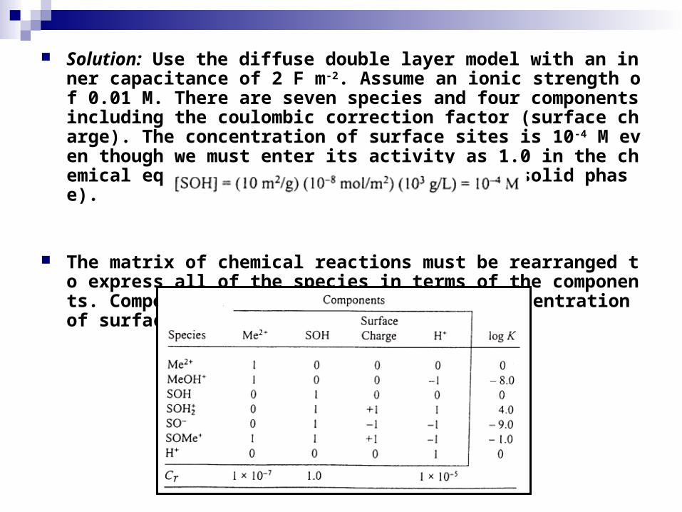
Solution: Use the diffuse double layer model with an inner capacitance of 2 F m-2. Assume an ionic strength of 0.01 M. There are seven species and four components including the coulombic correction factor (surface charge). The concentration of surface sites is 10-4 M even though we must enter its activity as 1.0 in the chemical equilibrium program (activity of a solid phase).

The matrix of chemical reactions must be rearranged to express all of the species in terms of the components. Components should include Me2+, the concentration of surface sites SOH, and H+.

Figure 8.25 shows graphical output from the model. a. The concentration of free aquo metal ion (Me2+) predominates at pH

≤ 5. Adsorbed metal concentrations are predominant above pH 6. At pH 5.5, the adsorbed and dissolved concentrations are equal.

b. The adsorption edge rises sharply from pH 5 to pH 7. Essentially all of the metal ion is bound at pH 7, so liming the soil would be an effective way to immobilize the metal ions.

c. The surface charge is zero at pH 6.5. Soil particles are positively charged due to adsorption of metal ions at pH 5.

d. The Kd values are strong functions of pH.

Figure 8.25 Chemical equilibrium model for metals speciation in a contaminated soil. Top: Equilibrium concentrations (M) as a function of pH Middle: Adsorption edge from pH 5 to 7. Bottom: Surface charge on the soil particles as a result or the surface complexation or hydrous oxides for metal cations.

8.8 CLOSURE

In this chapter, we have learned that chemical speciation drives the fate, transport and toxicity of metals in natural systems. We must combine mass balance equations with chemical equilibrium models to address these problems.

It is difficult to obtain all the desired model parameters and equilibrium constants, but a multiple approach or model calibration, collection of field data, microcosm experiments, and laboratory measurements will prove to be successful.

Considerable improvements in the state-of-the-art for waste load allocations of metals are needed to put regulatory actions on a more scientifically defensible basis.