a benchmarking platform for network-on-chip (noc
TRANSCRIPT

A BENCHMARKING PLATFORM FOR NETWORK-ON-CHIP (NOC)
MULTIPROCESSOR SYSTEM-ON-CHIPS
A Thesis
by
JAVIER JOSE MALAVE-BONET
Submitted to the Office of Graduate Studies of
Texas A&M University
in partial fulfillment of the requirements for the degree of
MASTER OF SCIENCE
December 2010
Major Subject: Computer Engineering

A BENCHMARKING PLATFORM FOR NETWORK-ON-CHIP (NOC)
MULTIPROCESSOR SYSTEM-ON-CHIPS
A Thesis
by
JAVIER JOSE MALAVE-BONET
Submitted to the Office of Graduate Studies of
Texas A&M University
in partial fulfillment of the requirements for the degree of
MASTER OF SCIENCE
Approved by:
Chair of Committee, Rabi N. Mahapatra
Committee Members, Riccardo Bettati
Paul Gratz
Head of Department, Valerie E. Taylor
December 2010
Major Subject: Computer Engineering

iii
ABSTRACT
A Benchmarking Platform For Network-On-Chip (NOC) Multiprocessor System-On-
Chips. (December 2010)
Javier Jose Malave-Bonet, B.S., University of Puerto Rico at Mayagüez
Chair of Advisory Committee: Dr. Rabi N. Mahapatra
Network-on-Chip (NOC) based designs have garnered significant attention from both
researchers and industry over the past several years. The analysis of these designs has
focused on broad topics such as NOC component micro-architecture, fault-tolerant
communication, and system memory architecture. Nonetheless, the design of low-
latency, high-bandwidth, low-power and area-efficient NOC is extremely complex due
to the conflicting nature of these design objectives. Benchmarks are an indispensable
tool in the design process; providing thorough measurement and fair comparison
between designs in order to achieve optimal results (i.e performance, cost, quality of
service).
This research proposes a benchmarking platform called NoCBench for evaluating
the performance of Network-on-chip. Although previous research has proposed standard
guidelines to develop benchmarks for Network-on-Chip, this work moves forward and
proposes a System-C based simulation platform for system-level design exploration. It
will provide an initial set of synthetic benchmarks for on-chip network interconnection
validation along with an initial set of standardized processing cores, NOC components,
and system-wide services.
The benchmarks were constructed using synthetic applications described by Task
Graphs For Free (TGFF) task graphs extracted from the E3S benchmark suite. Two
benchmarks were used for characterization: Consumer and Networking. They are
characterized based on throughput and latency. Case studies show how they can be used
to evaluate metrics beyond throughput and latency (i.e. traffic distribution).

iv
The contribution of this work is two-fold: 1) This study provides a methodology
for benchmark creation and characterization using NoCBench that evaluates important
metrics in NOC design (i.e. end-to-end packet delay, throughput). 2) The developed
full-system simulation platform provides a complete environment for further benchmark
characterization on NOC based MpSoC as well as system-level design space
exploration.

v
Para toda mi familia por su apoyo y paciencia incondicional. En especial a mis padres
Nydia y Ricarter, mis abuelas Maria Luisa y Aracelia, mi hermano Carlos, todos mis tíos
y primos, en especial a mi tío Luis por ayudarme con su mentoría profesional, mis
suegros Vicente y Juanita, mis cuñados Tito y Nadgie y su esposo Tomás y mi sobrino
Fernando Enrique.
Finalmente, muy espcialmente para mi esposa, Geydie. Gracias por creer en mi,
por tu paciencia y amor durante el arduo trayecto que hemos recogido juntos. Sin tu
amor y apoyo jamás lo hubiera logrado. Te amo.

vi
ACKNOWLEDGEMENTS
I would like to thank my committee chair and advisor, Dr. Rabi Mahapatra for his
guidance and support throughout the course of this research.
Thanks also go to my friends and teammates of the Embedded Co-design team,
Suman, Ayan, Jason and Nikhil, as well as my wife, Geydie, for all the hands-on work
during this research. Their help was key to the completion of this work.

vii
NOMENCLATURE
APCG Application Characterization Graph
CNI Core Network Interface
CTG Communication Task Graph
CUT Core Under Test
DAG Directed Acyclic Graph
DMTE Data Memory Transaction Engine
EEMBC Embedded Microprocessor Benchmark Consortium
FSM Finite State Machine
GALS Global Asynchronous Locally Synchronous
LS Latency Sensitive
MM Memory Manager
NOC Network on Chip
OCP Open Core Protocol
PE Processing Element
PID Process ID
PCB Process Control Block
SOC System on Chip
TGFF Task Graphs For Free
TS Throughput Sensitive

viii
TABLE OF CONTENTS
Page
ABSTRACT .............................................................................................................. iii
DEDICATION .......................................................................................................... v
ACKNOWLEDGEMENTS ...................................................................................... vi
NOMENCLATURE .................................................................................................. vii
TABLE OF CONTENTS .......................................................................................... viii
LIST OF FIGURES ................................................................................................... x
LIST OF TABLES .................................................................................................... xii
CHAPTER
I INTRODUCTION ................................................................................ 1
II PROBLEM ........................................................................................... 5
III NOC BENCHMARKING PLATFORM ............................................. 9
A. System Components and Architecture ..................................... 9
B. Platform Overview ................................................................... 13
C. Software System Services ........................................................ 20
IV BENCHMARKS .................................................................................. 30
A. Characterization of Benchmarks .............................................. 32
V CASE STUDIES .................................................................................. 44
A. Real Applications ..................................................................... 44
B. Synthetic Benchmarks .............................................................. 47

ix
CHAPTER Page
VI CONCLUSION & FUTURE WORK .................................................. 53
REFERENCES .......................................................................................................... 55
APPENDIX A ........................................................................................................... 58
APPENDIX B ........................................................................................................... 60
VITA ......................................................................................................................... 70

x
LIST OF FIGURES
Page
Figure 1 A Simple Core Network Interface ..................................................... 10
Figure 2 A Simple 5 Cycle Router Pipeline .................................................... 11
Figure 3 Common Network Topologies .......................................................... 12
Figure 4 NoCBench Execution Overview ....................................................... 15
Figure 5 The SPARC Core with CNI .............................................................. 17
Figure 6 On Chip Memory Core with CNI ...................................................... 18
Figure 7 The TGFF Core with CNI ................................................................. 18
Figure 8 Simple Two-Node CTG .................................................................... 19
Figure 9 Data Receive/Transmission Phase .................................................... 19
Figure 10 SPARC Core with Kernel Interface .................................................. 22
Figure 11 TGFF Core with Kernel Interface ..................................................... 22
Figure 12 Scheduler Architecture ...................................................................... 23
Figure 13 TGFF Scheduler Data Transmission Phase Pipeline ......................... 26
Figure 14 Memory Manager with Kernel Interface ........................................... 27
Figure 15 Memory Logical View ...................................................................... 28
Figure 16 Consumer Benchmark APCG Example ............................................ 31
Figure 17 Benchmark Metric Application Example .......................................... 34
Figure 18 Scenario PeakTL ............................................................................... 38

xi
Page
Figure 19 Congested Latency Scenario ............................................................. 39
Figure 20 Congested Throughput Scenario ....................................................... 39
Figure 21 Consumer Execution Time (s) ........................................................... 41
Figure 22 Networking Execution Time (s) ........................................................ 42
Figure 23 Impact of Background Traffic ........................................................... 45
Figure 24 Simulated Instructions per Second .................................................... 46
Figure 25 NOC Topology and IP Placement ..................................................... 48
Figure 26 Throughput Mesh vs Torus ............................................................... 49
Figure 27 Latency Mesh vs Torus ..................................................................... 50
Figure 28 Execution Time per Application (s) .................................................. 50
Figure 29 Flits Traversed per Router over Time (%): Mesh ............................. 51
Figure 30 Flits Traversed per Router over Time (%): Torus ............................. 52
Figure A.1 Consumer Throughput Characterization (B/s) .................................. 58
Figure A.2 Consumer Latency Characterization (ns) .......................................... 58
Figure A.3 Networking Throughput Characterization (B/s) ............................... 59
Figure A.4 Networking Latency Characterization (ns) ....................................... 59

xii
LIST OF TABLES
Page
Table 1 Simulator Feature Comparison .......................................................... 14
Table 2 Network Components and Configurable Parameters ........................ 16
Table 3 Tasks per Application ........................................................................ 35
Table 4 Communication Load per Core ......................................................... 36
Table 5 TX/RX Ratio per Core ...................................................................... 37
Table 6 Experimental NOC Configuration .................................................... 40
Table 7 Benchmark Characterization ............................................................. 43
Table 8 Benchmark Execution Results .......................................................... 47

1
CHAPTER I
INTRODUCTION
Network-on-Chip (NOC) based designs have garnered significant attention from both
researchers and industry over the past several years. The analysis of these designs has
focused on broad topics such as NOC component micro-architecture [1][2][3][4], fault-
tolerant communication, system memory architecture and system level issues (i.e. task
scheduling and mapping, real-time issues, low power noc). Nonetheless, the design of
low-latency, high-bandwidth, low-power and area-efficient NOC is extremely complex
due to the conflicting nature of these design objectives. The NOC must be co-designed
with other chip components and its design must be evaluated with a total system
perspective.
Benchmarks play an essential role in the process of system design exploration
and analysis. Previously, guidelines have been proposed to develop standard benchmarks
for NOC [5], yet this is a problem that still remains scarcely addressed. Classic
benchmarks fall short of a solution since they are application oriented and do not exploit
communication intensive architectures [6][7]. NOC-based systems are expected to have
more heterogeneous workloads with respect to computation and communication. Thus,
to characterize a NOC benchmark a standard, well-defined, set of metrics is needed that
measure the elements that define a NOC [5]. A benchmark designed for NOC-based
systems needs to quantify the performances of the following: 1) functional and storage
blocks with corresponding network interface (cores), 2) the interconnect infrastructure
(routers and links), and 3) the fully integrated system.
____________
This thesis follows the style of IEEE Transactions on Automatic Control.

2
Network-on Chips provide the underlying communication infrastructure that
allows effective integration of functional, I/O, and storage blocks. Latency, throughput,
reliability, energy dissipation, and silicon area requirements characterize such
communication-centric interconnect fabrics. For this reason, application driven workload
is essential to compare different designs and evaluate the system effects on performance
characteristics of the NOC. The variability of injection rates and traffic patterns in real
applications provide an excellent opportunity for implementing adaptive hardware in
NOC.
Real benchmarks are the most accurate approach for application driven work
load, but their simulation is time intensive. Synthetic benchmarks conversely mimic real
program workload by extracting the communication characteristics of the application
into a communication task graph (CTG).
Ogras et. al provide a formal definition of a CTG. A Communication Task Graph
(CTG) G’ = G’(T, D) is a directed acyclic graph, where each vertex represents a
computational module in the application referred to as task ti ∈ T . Each task is
annotated with relevant information, such as execution time on each type of Processing
Element (PE) in the network, task i energy consumption ( ) when executed on the j-th
PE, individual task deadlines (dl(ti) ), periodicity of the task graphs, etc. Each directed
arc di, j ∈ D between tasks ti and tj characterizes either data or control dependencies.
Each has associated a value, which stands for the communication volume (bits)
exchanged between tasks ti and tj [8].
Synthetic benchmarks could also be reduced in scope (e.g. micro-benchmarks)
and impose the workload on a single component, thus isolating the measurement of
specific parameters.
Overall a benchmarking environment should cover the following aspects in a
NOC: 1) Packets and Transactions (Delay, bandwidth, jitter, power consumption of
individual packets and routing, switching, buffering, flow control of the network) 2)
Congestion (Arbitration, buffering, flow control) 3) Temporal and Spatial Distribution

3
(burst traffic scenarios, hot spot pattern detection) 4) Quality of Service (guaranteed
throughput and latency). 5) Network Size (scalability of communication network).
Due to the complex nature of these metrics NOC benchmarks cannot be
composed just of a specified application and data input set or a synthetic communication
task graph (CTG) alone. The same task set, or application mix, running on different
system configurations may potentially generate different traffic patterns, therefore being
characterized as distinct benchmarks. Network Size, core composition (i.e. processor,
memory, other IP) and task mapping must be part of the benchmark configuration. It is
necessary, then, to have a full benchmarking environment that is able to support this.
The scope of this thesis is to provide a benchmarking platform for network-on-
chip. It serves a dual purpose: 1) provides an environment for NOC benchmark
characterization, 2) Permits NOC based MpSoc design space exploration.
The platform includes an initial set of standardized processing cores, NOC
components, and system-wide services. System-C[9] is used as the main simulation
engine. The processing cores are capable of running standard benchmark applications to
generate network traffic. The platform also provides for NOC and system researchers to
easily plug-and-play existing components, or newly designed components, into a full
SoC. This allows a system designer to easily assess the quality of their ideas and designs,
to catch bottlenecks early in design formulation, and to study the relationship between
NOC architecture and application performance.
This research also addresses methodology issues in the creation of benchmarks.
An initial set of example synthetic benchmarks will be given along with the simulator.
They were constructed using TGFF task graphs from the E3S benchmark suite. In this
benchmark suite task execution time, communication dependencies (i.e. payload size,
task source and sink), application period and deadlines are extracted from execution of
EEMBC benchmarks on a series of processor models. This brings better accuracy to
these synthetic benchmarks in term of traffic generation compared to random traces or
manually constructed communication task graphs. We discuss mapping techniques of the
applications into different system configurations, in order to create distinct traffic

4
scenarios in the communication network that will evaluate important metrics in NOC
design (i.e. end-to-end packet delay, sustainable throughput).

5
CHAPTER II
PROBLEM
In the SoC design cycle validation and verification is a process that persists throughout
all the steps, from architectural design to physical design and the manufacturing process.
Nonetheless, while NOC based MpSoC designs have been proposed for years; they are
just being introduced into the market [10][11]. The research community is still facing
obstacles to find proper validation and verification schemes for the initial design stages.
One of the main problems associated with NOC based research and development, as
proposed by Grecu et al [5], is the lack of suitable benchmarks.
Previously Grecu et. al [5] provided a general categorization of NOC
benchmarks. In addition to real programs, micro-benchmarks and synthetic applications
they also address definitions of benchmarks for fault tolerance and reliability.
For synthetic benchmarks they proposed that a NOC benchmark has to be
applied on more than a simple topological description, but rather on a combination of
functional IP cores and NOC components with a certain system architecture (i.e.
topology), and specific information of traffic patterns running on the on-chip network
communication architecture. The superposition of these various elements creates
different benchmark scenarios. Moreover, these scenarios are used to characterize the
benchmark. They provide a methodology that imposes a CTG on processing elements
and establishes an FSM for PE execution. They suggest two metrics for measurement:
application execution time and application throughput.
In previous work Ogras et. al define such a mapping as an application
characterization graph (APCG). An Application Characterization Graph (APCG) is a
directed graph G =G(C,A), where each vertex ci C represents a selected IP/core, and
each directed arc ai,j characterizes the communication process from core ci to core cj.
Each ai,j can be tagged with application-specific information (e.g. communication
volume, communication rate, etc.) and specific design constraints (e.g. communication

6
bandwidth, latency requirements, etc.). Also, the size/shape of cores ci C is assumed to
be known [8].
Overall we subdivide the problem of NOC benchmarking into three further sub-
problems: Application Selection or Modeling, Benchmark Creation and Characterization
and Simulation Environment Development.
Application Selection and Modeling addresses the usage of real programs and the
creation of CTGs for synthetic applications. There are several benchmark suites that are
widely used and known among the research community such as: miBench, SPEC,
Alpbench, EEMBC among others.
In order to create communication task graphs a widely accepted tool has been
used among researches called Task Graphs For Free (TGFF). TGFF lets the user create
task graphs with detailed information in terms of task definition, communication
requirements and dependencies. Users may specify parameters for a task such as code
size, data communication volume, task period and processor specifications (i.e.
architecture, price). Task graphs created are directed acyclic graphs (DAG) and are
equivalent in definition to a CTG. Each node represents a task and an arc between each
node represents a directed dependency (source to sink) between them.
The E3S benchmark suite has gathered information from the Embedded
Microprocessor Benchmark Consortium (EEMBC) suite to create a benchmark suite for
use in system synthesis research. It is particularly useful in terms of automated system
allocation and mapping as well as scheduling research. E3S has characterized several
well known processors from AMD, Analog Devices and Texas Instruments. Task graphs
used for this characterization are given with realistic detailed information of EEMBC
task’s execution time (per given target architecture), communication data volume, code
size, deadlines and periods. TGFF was used to built the CTG and provide task
communication dependencies. The E3S benchmark suite also provides instructions for
creating additional CTG’s. Although, not a real substitute for real applications, this
synthetic benchmarks model realistic application data using real world applications and
systems.

7
Simulation and Environment Development addresses the creation of a suitable
platform for the creation, characterization and execution of benchmarks. Noxim is a
flexible SystemC-based NOC Simulator that models systems organized in a 2D mesh
topology [12]. Noxim evaluates NOC characteristics through synthetic traffic generation
(e.g. stochastic probabilistic traffic) – injection distribution, destination distribution and
injection rate can be specified by the user.
Garnet [13] is a network-on-chip performance simulator which is compatible
with the GEMS [14] multiprocessor framework along with Simics [15]. It can be
interfaced with the Orion [16] network-on-chip power modeler when necessary. Garnet
provides two modes of operation: a detailed “fixed pipeline” mode, and a high-level
“flexible-pipeline” mode. The fixed-pipeline mode models the micro-architectural
details of the on-chip router, while the flexible-pipeline mode allows the user to
parameterize the number of router pipeline stages, and simply delays network traffic by
that many cycles per router. Although Garnet is an excellent tool due to its accuracy and
inter-operability with other system-level simulators, it does not provide full end-to-end
models of the NOC (e.g. CNI, other infrastructure IP) within a single framework.
Additionally, only 2D-mesh topologies can be modeled with the Garnet simulator.
NIRGAM is a SystemC-based NOC simulator that allows a user to model a mesh
or torus NOC [17]. Traffic is generated either synthetically or through a traffic trace.
Like the other NOC simulators mentioned, NIRGAM also allows a user to vary certain
NOC component parameters, such as buffer depth, number of virtual channels, and
routing algorithm.
Although each of the simulators discussed above are well suited for specific
purposes, there is still a need for a simulation platform that encompasses all the needs of
a NOC benchmarking environment. That is modeling a complete flexible system capable
of simulating all varying types of benchmarks (i.e. real code, synthetic applications,
micro-benchmarks). The main shortcoming of all the simulators discussed above is, they
either simulate the network or the cores. NoCBench is the first step towards bridging the

8
gap by providing a full system simulation environment equipped with cores, network
components and a simulated kernel.
To the best of our knowledge there is no work addressing the creation and
characterization of benchmarks. In this work we address synthetic applications and use
the E3S benchmark as a starting point. We address the methodology of characterization,
selection of metrics and their usage for studying NOC problems.

9
CHAPTER III
NOC BENCHMARKING PLATFORM
A. System Components and Architecture
1. System on Chip
Modern embedded systems are often composed of many IP blocks including processors,
memory blocks, DSPs and controllers. Traditionally these blocks have been connected
using direct wiring or on chip buses. However, with growing integration and shrinking
device size and increased chip size, wiring delays are becoming significant. Also, as we
pack more cores and connect with buses, contention becomes a major bottleneck. To
address these network on chip has emerged as a solution for communication on the
chip[18][19]. Details of the Network on Chip architecture is discussed here.
2. NOC Architecture
Network on Chip architecture is inspired by the asynchronous communication paradigm
of packet switched computer networks. With increased on chip wiring delay
synchronized communication between the far ends of a large system on chip is
impractical. Network on Chip tries to address this issue by introducing a globally
asynchronous locally synchronous (GALS) paradigm. In NOC, communication takes
place between cores using information packets. Packets are generated at the source and
carried to the destination by intermediate routers. At the destination, the packet is
decomposed into data and processed by the receiver. Clearly NOC architecture will have
the following components. A Core to Network interface, Routers and Links. The
following sections discuss the functional and architectural details of these components.

10
3. Core Network Interface (CNI)
The Core Network Interface, or CNI, is the functional equivalent of a network card in
standard multi-computer systems [2]. The CNI connects the IP cores to the network. Its
primary job is to translate the raw information generated by the core into packets to be
transmitted through the network and the reverse process for packets coming in from the
network. The CNI also performs address resolution to find the destination core based on
the address in the incoming request. In addition, a CNI can also perform system
management tasks such as power management, fault detection, core test support, and
system reconfiguration. The block diagram of an example CNI is given in Figure 1.
Figure 1: A Simple Core Network Interface
The CNI architecture assumed in this research provides simple traffic translation
to enable inter-core communication across the network-on-chip. For more complex
systems, other functionality may be added to this base model as necessary. Other
researchers present a thorough examination of additional functionality that may be added
[2][3].
4. Router
The on-chip router is the most salient component in a Network on Chip. Similar to
standard computer networks, the router’s job is to efficiently route packets through the
11
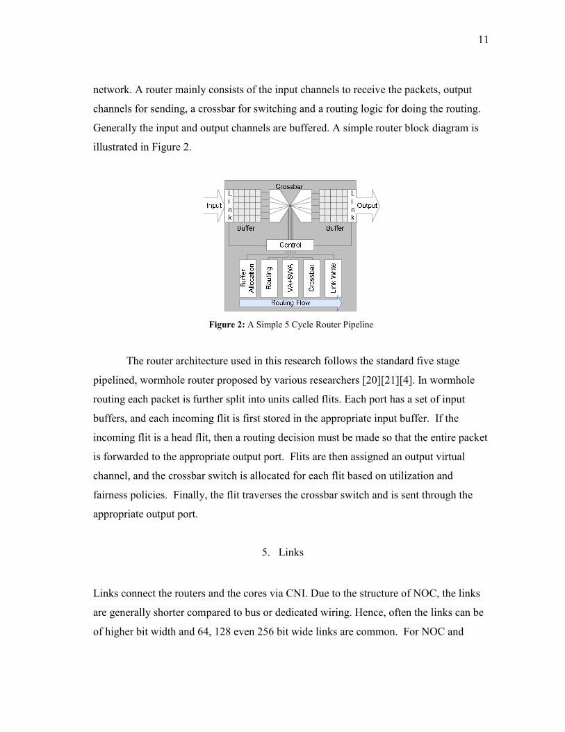
network. A router mainly consists of the input channels to receive the packets, output
channels for sending, a crossbar for switching and a routing logic for doing the routing.
Generally the input and output channels are buffered. A simple router block diagram is
illustrated in Figure 2.
Figure 2: A Simple 5 Cycle Router Pipeline
The router architecture used in this research follows the standard five stage
pipelined, wormhole router proposed by various researchers [20][21][4]. In wormhole
routing each packet is further split into units called flits. Each port has a set of input
buffers, and each incoming flit is first stored in the appropriate input buffer. If the
incoming flit is a head flit, then a routing decision must be made so that the entire packet
is forwarded to the appropriate output port. Flits are then assigned an output virtual
channel, and the crossbar switch is allocated for each flit based on utilization and
fairness policies. Finally, the flit traverses the crossbar switch and is sent through the
appropriate output port.
5. Links
Links connect the routers and the cores via CNI. Due to the structure of NOC, the links
are generally shorter compared to bus or dedicated wiring. Hence, often the links can be
of higher bit width and 64, 128 even 256 bit wide links are common. For NOC and

12
system benchmarking purposes, all data flowing through links is assumed to require one
cycle of latency.
6. NOC Topologies and Routing
A NOC can have different topologies and routing algorithms depending on application
needs and available resources. We will discuss the most common and widely used
topologies and routing algorithms in the following sections.
7. Topology
The most commonly used topologies in NOC research are 2D Mesh and Torus
topologies. However, other interesting topologies such as butterfly, fat-tree, and
Gaussian networks have also been proposed [22]. The mesh and torus topologies are
favored due to their regular structure and planar geometry and simplicity.
Figure 3 illustrates the three common topologies, namely Torus, Mesh and Irregular.
Figure 3: Common Network Topologies
System designers must select the appropriate topology for their expected
application requirements, based on topological metrics such as link density and network
diameter.

13
8. Routing
Routing in NOC depends on the topology. It can be table lookup based where each
router has next hop information for every destination in the network or it can be
geometry based like dimension ordered or XY routing. The third type of routing is called
source routing, where the sender specifies all the intermediate nodes in the packet. Each
routing technique differs in performance with respect to adaptability, average hop count,
and flit header storage requirements. The performance of the system can vary greatly
depending on the routing technique used.
B. Platform Overview
The proposed platform, NoCBench, consists of a flit accurate network on chip simulator.
The simulator can be configured according to system needs and it can support a variety
of architectures (i.e. multiple core-network interface link configuration, switching
policies, topologies). In this section we describe the simulation environment.
Table 1 compares the features and capabilities of the NOC simulator described in
this research. ISS Integration is the capability of the NOC simulator to use real
application behavior as a basis for NOC traffic. Our NOC platform includes the ArchC
ISS to model core behavior, while Garnet interfaces with Virtutech Simics to provide
core functionality. The other simulators do not provide this capability. Topologies is
the allowable set of NOC topologies supported by each simulator. Flit Accurate is the
level of accuracy supported by each simulator. The Parameterized NOC feature means
that the simulator supports user-configurable routing algorithms, buffer depths, number
of VCs, etc.

14
Table 1: Simulator Feature Comparison
1. NOC Simulator
The included NOC simulator is a flit accurate network on chip simulator written in
SystemC. It makes use of the SystemC simulation engine and behavioral level network
component library for fast simulation. Figure 4 shows the organization of the NOC
simulator in the platform. The Simulator consists of the following main units: the NOC
generator, the component library, and the simulation engine. The NOC simulation
environment is compatible with any SystemC simulation engine. In our evaluation we
have used the OSCI SystemC simulation engine. It is capable of very fast and accurate
simulation in any platform and it is fully open source.
Features NoCBench Gems – Garnet Nirgam Noxim
ISS Integration Yes - ArchC Yes – Simics No No
Topologies Full Custom Full Custom Mesh, Torus Mesh
Flit Accurate Yes Yes Yes Yes
Power
Measurements Yes – Router/CNI/Global Yes – Module Level No Yes
Fault Injection Yes No No No
Parameterized NOC Yes Yes Yes Yes
Full System Yes Yes No No
Open Source Yes Dependent on Simics Yes Yes

15
Figure 4: NoCBench Execution Overview
2. Network Generator
This module reads a configuration file specified in XML format and generates the NOC
using SystemC library modules. The configuration includes the topology, specification
of parameters for the CNI, Router and Links. It can also specify fault simulation
parameters, and the configuration can be extended according to the need for
specification of additional properties. An example configuration can be found in the
Appendix.
3. Network Component Library
The network component library is the core of the simulation system. In this library we
have modeled the components of the NOC using SystemC. The router and the CNI can

16
be configured to implement popular peak power management schemes like PowerHerd
[20] and PC [21]. The system level model allows for fairly accurate and much faster
simulation compared to detailed RTL simulation. Table 2 provides the details for the
available modules in the network component library.
Table 2: Network Components and Configurable Parameters
Component Configuration parameters
CNI Flit injection rate, message queue length.
Router Number of ports, buffer lengths, number of virtual channels.
Routing XY routing, table based routing, source routing.
Link Bit widths.
4. Configurable Core Library
The configurable Core library provides SystemC models of IP cores. We have three
types of core models in this library in the current version of the NOC platform.
Synthetic Cores: These cores can generate communication based on statistical
traffic distributions. These types of cores do not generate meaningful traffic in the
network and do not necessarily perform meaningful communication. However, these
cores can be configured to produce network traffic that follows the expected high-level
behavior in the network, which allows for generalized performance benchmarking of
NOC components. Statistical random number generators are used to mimic traffic
distributions. Examples of statistical traffic patterns include uniformly distributed
network traffic and self-similar traffic models.
Real Cores: These are SystemC wrapped cores, typically implemented in either
C++/C. The most common examples of these core implementations are instruction set
simulators (ISS) for different processing cores. They also include cache and memory
models. We have used ArchC [23] based processor models to represent real cores.
ArchC is an open-source language written in SystemC used for processor architecture
description. It generates functional and cycle accurate ISS using Instruction Set
Architecture (ISA) for popular embedded processor models like MIPS, Intel8051,

17
SPARCV8 and PowerPC. The architecture chosen for integration is SparcV8 since it is
well known and widely supported, as show in Figure 5. It has a 7-stage pipeline, separate
configurable caches and comes with a compiler tool chain.
Figure 5: The SPARC Core with CNI
The core has a structural, SystemC top module while the internal functions are
implemented in a functional C++ model. We have augmented the top module to inherit
from a generic OCP (Open Core Protocol [24]) core to act as a master providing a
compliant port for communication with the CNI. The OCP port is connected internally to
a soft arbiter that handles incoming/outgoing requests. This soft arbiter serves for future
expansions (e.g. Interrupt Control). The core also implements a System C wrapper
around the cache controller to prepare the requests to be sent to the remote memory core.
The soft arbiter and the wrapper work together to synchronize request and responses. In
addition to the Sparcv8, our platform includes an on-chip memory model. The on-chip
memory model is a soft implementation of the block. The modularized nature of the
models allow the user to readily experiment with memory and cache sizes and other
characteristics to discover the most efficient implementation for a given system. Figure 6
shows the block diagram of the memory model included in this version of the
NoCBench tool.

18
Figure 6: On Chip Memory Core with CNI
TGFF Cores: These cores were used to characterize the synthetic benchmarks.
They generate traffic based on information obtained from a DAG. Figure 7 illustrates the
TGFF core architecture. They execute synthetic tasks which have defined
communication dependencies, communication volume, task period and task deadline. In
this sense, a TGFF core is an abstract representation of the intellectual property (IP)
block the task was modeled from. Each task in the graph is a source, sink or both with
respect to another task. The weighted arc between the two defines the communication
dependency and volume. Figure 8 show a simple Task graph with two nodes. The core
connects to CNI in a similar fashion than real cores. A master and a slave interface are
connected to request and accept transactions respectively.
Figure 7: The TGFF Core with CNI
TGFF CORE
CNI
O
C
P
Control
DMTE
OC
P W
rap
per
fo
r
TG
FF

19
Figure 8: Simple Two-Node CTG
Each task is modeled by the TGFF core in two phases: Data Transmission, and
Data Reception. A task’s job is finished when both phases have been executed.
Data Transmission & Data Reception: Data packet transmission is simulated by
the Data Memory Transaction Engine (DMTE) using the communication volume and
dependencies specified by the user for the task. The entire communication volume must
be sent for each destination task, or sink. The DMTE creates an OCP packet per cycle
for each sync in a “best effort” fashion, and pushes it into a transmit pending queue. The
master interface pops one packet every cycle if CNI is available. CNI then injects the
packet into the network. The core injection rate will depend on the network parameters
(i.e. flit size, message queue length). The theoretical rate is 1 packet per cycle. The
maximum payload size then determines how many packets need to be sent by the core in
order to send the entire communication volume specified by the task.
Figure 9:Data Receive/Transmission Phase
The Data Transmission phase starts when the first packet has been sent and ends
when the last packet has been given to CNI. The Data Transmission phase may not start
until Data Reception is done. The Data Reception phase ends when the last packet has
been received from all sources. Data is received from the CNI through the slave
interface. Figure 9 illustrates the data phases.
SRC SINK
Data Volume
DATA RX DATA TX

20
TGFF cores could be expanded to improve its modeling capabilities by the
addition of parameters such as core size (e.g. pipeline width) and power consumption
(i.e. ratios of instructions types and their average power consumed). Further modeling
discussions are discussed in later sections.
Controller and Statistics: The controller keeps track of all packets sent and
received. It gathers transmit and receive throughput statistics per task, aggregated
transmit and receive throughput per core as well as average core to core latency per task
and per core. The controller also communicates with the system kernel to notify when
the task is done. This is explained in section C.1.
Simulation Engine: The NOC simulation environment is compatible with any
SystemC simulation engine. In our evaluation we have used the OSCI SystemC
simulation engine. It is capable of very fast and accurate simulation in any platform and
it is fully open source.
C. Software System Services
The NOC platform includes a light kernel to provide simple system services. The kernel
itself is a service provided by the platform and it is simulated in the host machine. It is
modeled as a soft System-C module which provides sufficient accuracy without much
simulation time overhead. The primary services are: scheduler, memory manager and
system call support. The kernel provides an interface to communicate with each IP core.
The interface is presented in detail in the following section.
1. Core Interface
The core interface is a pivotal part of the platform. It is the kernel’s job to support all
indispensible system services expected by applications running on the platform. At the
same time, this must not imply excessive modification of the core model (i.e. ISS, RTL
module) in order to be ported. To achieve this ease of portability, the kernel centers

21
around one data structure: the process control block (PCB). All software information
regarding system control would be communicated through the interface by the PCB. The
PCB emulates the same features that process control blocks of real operating systems
have:
1. Program Address Space
2. Local to Global Address Translation
3. Process Id (PID)
4. Heap and Argument pointers
5. Process status
Additional information for platform run-time management includes:
1. Target Architecture (i.e. sparcv8, arm, etc.)
2. Core Id currently running on
3. Number of Jobs
Of course, register information is target dependent and cannot be abstracted in a
generic data structure. That information still remains in the ISS and its management
remains separated from the kernel system. It is the interface job to close the gap. The
interface consists of four control functions: Start(), Stop(), Yield() and Notify(). The first
three are expected to be implemented by the core (i.e. ISS) and are driven by the kernel
while Notify() is driven by the core and is provided by the system library. These
functions, illustrated at Figure 10, are described in detail below.
1. Start(): Takes in PCB and initializes all pertinent data (i.e. PC register, IC and
DC invalidation). Processor is released from stall and begins (or continues)
execution.
2. Stop(): Does not have any inputs. Stalls the processor.
3. Yield(): Takes in PCB from new process. Signals context switch.
4. Notify(): Takes in PID. Provides Kernel scheduling pertinent information (i.e.
process status)

22
Figure 10: SPARC Core with Kernel Interface
TGFF cores, however, have an interface of their own with the kernel, illustrated
at Figure 11:
1. Set_process(): starts the Data Reception phase and initializes all parameters
2. Start(): starts the Code Processing and Execution Phase immediately. Data
Transmission is triggered internally by the core when appropriate.
3. Notify(): Takes in PID. Provides Kernel scheduling pertinent information (task
status)
Figure 11: TGFF Core with Kernel Interface
TG
FF
CO
RE
Control
TG
FF
SY
ST
EM
IN
TE
RF
AC
E System
Kernel
+
TGFF
Scheduler start()
set_process()
stop()
DMTE
notify()
data volume
notify_done
sources
sinks
CORE
Co
re-K
ern
el I
nte
rfac
e
System
Kernel
stop()
start(PCB)
yield(PCB)
notify(PCB)
Sparcv8 Instance

23
2. Scheduler Framework
The scheduler is one of the most important modules for studying the impact task
mapping has on overall system performance, meeting task deadlines/guarantees, on-chip
network traffic load, and power consumption. Thus, a solid foundation was built to allow
researchers to easily integrate their scheduling algorithms into the rest of the platform.
Overall, the scheduler is built on top of task handlers defined as queue data structures
and interacts with a loader and the memory manager to implement a given algorithm.
3. Scheduler Setup and Architecture
Setup: The scheduler framework has two programmable parameters: tick and scheduler
type. These two parameters are passed through the XML configuration file.
Architecture: As shown in Figure 12, at each tick the scheduler module will start
the scheduler algorithm specified by the user. Each algorithm uses a given set of queues
to manage the tasks. The queues will only hold the PID of a task as information. Queues
may be defined in terms of priority as well as task status (i.e. preempted or ready). The
scheduler framework interfaces with the Memory Manager to ask for memory allocation
and freeing.
Figure 12: Scheduler Architecture
Scheduler Algorithm
@tick
Task Queues
Memory Manager
Po
p()
All
oc
Free()
-Insufficient
Memory -Task Done
-Task Not Ready

24
To preempt a task the scheduler algorithm must drive the Yield() function for a
specific core to signal a context switch. As mentioned in the previous section, register
information and management is target dependant. Therefore, it is the core’s job to
implement its own save context and restore context method. Having this data stored at
the PCB structure will incur in a data and control overhead without any value added in
terms of simulation accuracy. Also, most architectures have readily available code for
this functions which makes them easy to port. Register information is not actually stored
in the PCB stack in memory but at the simulator’s memory space in the host machine.
This lowers simulation overhead in terms of memory transactions at the expense of
application timing accuracy.
The system supports ELF binaries only. An ELF loader is invoked for every task
the first time it needs to be loaded into main memory. For every task’s new job (or
resuming of a job) the loader is not invoked unless its memory had to be freed for
another task to run. Memory allocation/deallocation is explained in more detail in the
next sections as it is the memory manager’s job. However, it is the scheduler’s job to
manage resource allocation and to ensure that sufficient memory is available for the next
task.
4. Algorithms
Currently two schedulers are provided with the platform: a Round Robin (RR) scheduler
and a TGFF dedicated scheduler.
Round Robin: The RR scheduler manages the tasks as a typical circular list and
serves each task in a first come first serve manner. The RR scheduler algorithm uses two
queues: ready_tasks queue and preempted_tasks queue. The ready_tasks queue holds the
PID’s of all tasks whose previous jobs have completed and are ready to run (i.e. all
dependencies have been met). The prempted_tasks queue holds the PID’s of all tasks
whose current jobs have not completed and where preempted in the previous scheduler
invocation. This version of the RR scheduler uses the preempted tasks queue to give

25
higher priority to previously preempted tasks. At each tick each core is examined. If the
core is free (i.e. idle) it pops a task from the preempted tasks queue and its current job is
resumed on this core. If the core is busy then the task currently running on the core is
preempted and is pushed into the preempted tasks queue. For each task in the ready tasks
queue a new job is spawned only if all preempted tasks have been scheduled (i.e.
mapped to a core) and there are cores still available.
TGFF Scheduler: This is an online dedicated scheduler for the modeling of
TGFF task graphs. It was the scheduler used for the creation of the benchmarks
provided. The TGFF scheduler receives a series of application characterization graphs
(APCG) from the configuration as defined in section 3.3. Section 4 explains how APCG
are created. The scheduler must enforce all communication dependencies, therefore
when a task is scheduled to run, all its sinks must be scheduled on their respective cores
as well. This is because communication between tasks happens from core to core;
therefore all tasks pertaining to the communication must be scheduled. It is important to
note that this not a hardware-software co-design problem. In this regard, whether the
tasks can be implemented as hardware blocks with direct communication (i.e. a video
co-processor with a network packet accelerator) or as soft tasks communicating through
shared objects in memory, it is of little importance to the scheduler. The main scope is to
create benchmarks that will stress and evaluate the on-chip network communication
infrastructure.
To ensure proper scheduling, the algorithm locks all cores requested by an APCG
as soon as there are available. This has a drawback though. Since all tasks must receive
all data and finish execution before their data is ready to be injected into the network,
this scheme translates into very low traffic injection from each APCG. A possible
enhancement is to lock only the cores for a specific task and its respective sinks, leaving
more cores available for other APCG in wait. However, due to the nature of the
communication task graphs from E3S, this still did not stress the NOC enough and
creates unattractive scenarios. To solve this, we schedule the tasks in a pipeline fashion.
The scheduler assumes, previous jobs of each tasks have already run therefore

26
the task may start its Data Transmission phase as soon as it starts; leading to appropriate
data parallelism in the NOC. Figure 13 shows the pipeline execution model.
Figure 13: TGFF Scheduler Data Transmission Phase Pipeline
5. Scheduler Expansions
Real-time scheduling algorithms can easily be added by adding the necessary priority
information to the PCB such as: period, deadline and/or QoS requirements. The queues
structure is easily expandable as well to incorporate as many priority queues are
necessary. Since only PID needs to be tracked at the priority queues, this expansion is
straightforward.
6. Memory Manager
The memory manager (MM) and the scheduler are the backbone of the kernel. It is the
MM’s responsibility to address loading of binaries into memory by allocating and
mapping the local address space of the task into the global address space of the entire
system. The MM is also responsible for online bookkeeping of the memory consumed
by each process.
7. MM Setup and Architecture
The MM implements a two-level paging system. The MM has the following
programmable parameters:
1) Page Table Size
DATA RX DATA TX
DATA RX DATA TX
DATA RX DATA TX
Job1
Job2
Job N

27
2) Page Size
When the system is first instantiated it is given by the Network Generator the
physical space available for memory. The MM then partitions this space into a global
memory map consisting of the following sections:
1) Instruction Memory
2) Heap and Stack
3) Shared Memory
4) Process Arguments
Figure 14 shows the MM interface with the scheduler. As described above the
ELF loader is invoked by MM when driven by the scheduler. At this point all sections of
the process are extracted. Each process section (e.g. text, .bss, stack, heap and
arguments) is appropriately mapped to a corresponding section in global memory. The
granularity of a task memory view is a page. Figure 15 shows the logical view of the
memory architecture.
Figure 14: Memory Manager with Kernel Interface
Mem Manager
System
Kernel
allocMem(PCB)
freeMem(PCB)
Mem
-Ker
nel
In
terf
ace
ELF Loader
Invoke Loader

28
Figure 15: Memory Logical View
(Left: Process Space, Center: Global Memory, Right: Physical Core)
8. Problem Explorations with MM
The NoCBench kernel provides the proper framework and support for researchers to
evaluate many NOC scheduling and memory architecture related problems.
For example, it is important to note that the MM is oblivious to the memory architecture
in hardware. In other words, it does not take into consideration how many RAM
cores/banks are present in the system and their respective placement in the NOC. This
effectively creates a fragmentation problem in global space. At allocation, the local
address space could be spread out through the NOC depending on the amount and
location of memory cores. Furthermore, memory bookkeeping is done in terms of pages
released. When memory is freed the MM cannot keep track of these pages' correlation to
the memory cores potentially creating more fragmentation. Specifically for NOC this
creates an issue. Where a task is scheduled (e.g. in which core is it running) and how it is
partitioned (e.g. where its memory is stored) affects tremendously the traffic load in the
on-chip network, which ultimately affects the task's performance. Real-time analysis
also becomes more problematic when unquantifiable fragmentation happens.
NoCBench is also a great platform to study the potentials of Non-Uniform Cache
Architectures as well as to explore cache-coherence designs on Network-on-Chip.
Proc N Global M
Proc 1
.text
.data
.bss
.heap + .stack
.shrd mem
.args space
Prog.
Mem
Heaps +
Stacks
Shared
Mem
Args.
Space
Mem C0
Mem C1
Mem C2
Mem CN

29
9. System Calls
Simulation of system calls could be quite complex and take up many cycles to execute.
In a real system implementation of system calls is target dependant. Some architectures
provide a register to be written by software with the number of the system call to execute
and use a software interrupt to signal the transfer to the OS. This is typical in RISC
architectures. Others, like X86, use special instructions that identify a system call. This
transfer mechanism alone will create quite a performance overhead. Therefore, we
follow the trapping and host forwarding emulation mechanism implemented in the
ArchC Sparcv8 ISS. The ArchC project provides a cross-compiler for Sparcv8 binaries
in which system calls are given a pre-defined address in Instruction Memory. At run-
time the PC is tracked and when it reaches on the pre-defined addresses the system call
(i.e. srbk()) and corresponding data are forwarded to the host machine for execution.
When required, data is read back into the memory models and execution is resumed.
This method penalizes timing accuracy in favor of simulation speed, but it remains a
popular system call support mechanism since the impact is small [25].
In order to support any Sparcv8 cross-compiler a modification to the trapping
mechanism could be done as done by [25]. Instead of assigning pre-defined addresses to
the system call symbols the addresses could be fetched dynamically when the loader is
invoked and passed to the core through the Core-System interface when the task is
started.

30
CHAPTER IV
BENCHMARKS
The design of SoC’s is a complex iterative process where application requirements are
an important factor in the decision of parameters, components and software used in the
system. Although applications must conform to system limitations, the system design
must strive to comply with the minimum expectations of the application domains it is
being marketed for. For example, a telecommunications application to be run on a
cellular base station implementing LTE standard requires a minimum bandwidth from
the SoC communication architecture else the system would be useless for the application
at hand [26]. Therefore, it is important to establish the sustainable throughput and
minimum core to core latencies in the system. Addressing the scalability of NOC
components, routing and load balancing schemes as well as topology selection is part of
this process. Once this is validated an application designer can address software issues
such as scheduling and task mapping. Nonetheless, our goal in benchmark creation is not
to address the holistic design issues of SoC, but to create scenarios that efficiently
validate approaches to known on-chip network problems.
NoCBench includes a set of synthetic application benchmarks. These
benchmarks are intended to be an initial effort. They serve to discuss the methodology of
developing benchmarks with NoCBench. The synthetic application benchmarks have
been created using derived information from the E3S benchmark suite. Each E3S
benchmark has a series of applications, defined as communication task graphs (CTG).
Hereafter we will address CTG as application. E3S follows the same organization of the
EEMBC benchmark suite where each suite is categorized as: automotive/industrial,
consumer, networking, office automation, and telecommunications. Before we go into
further detail of how NoCBench benchmarks were characterized we will introduce and
discuss important definitions used in this process.
31
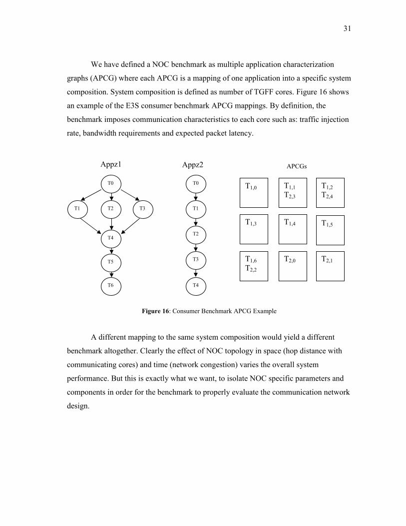
We have defined a NOC benchmark as multiple application characterization
graphs (APCG) where each APCG is a mapping of one application into a specific system
composition. System composition is defined as number of TGFF cores. Figure 16 shows
an example of the E3S consumer benchmark APCG mappings. By definition, the
benchmark imposes communication characteristics to each core such as: traffic injection
rate, bandwidth requirements and expected packet latency.
Figure 16: Consumer Benchmark APCG Example
A different mapping to the same system composition would yield a different
benchmark altogether. Clearly the effect of NOC topology in space (hop distance with
communicating cores) and time (network congestion) varies the overall system
performance. But this is exactly what we want, to isolate NOC specific parameters and
components in order for the benchmark to properly evaluate the communication network
design.
T0
T1 T2 T3
T4
T5
T6
Appz1
T0
T1
T2
T3
T4
Appz2
T1,0 T1,1
T2,3
T1,2
T2,4
T1,3
T1,4
T1,5
T1,6
T2,2
T2,0
T2,1
APCGs

32
A. Characterization of Benchmarks
This section discusses the methodology for creating benchmarks on NoCBench. It
addresses the mapping of applications into APCG, metrics used in the characterization of
our benchmarks and the experimental setup used to characterize each benchmark.
1. Methodology
The methodology followed in the creation of our benchmark is composed of a series of
well defined steps. These steps are:
1) Mapping of applications into APCGs,
2) Metric selection for categorization of a benchmark,
3) Measurement points selected to extract metric values
4) NOC parameter configuration – topology, router parameters, CNI parameters
Step 4) is tightly related to experimentation setup so it would be explained in the
experimental setup section. Nonetheless, it is an important step in our methodology.
Mapping Application to an APCG: When mapping an application the first step is
to select the number of TGFF cores to be used. The number of cores gives the size of the
benchmark and sets a lower bound on the load imposed on the NOC. Naturally an
application with N bytes of data to communicate would stress the NOC differently when
distributed among different number of cores. In the current version of NoCBench the
number of cores needs to be at least the maximum number of tasks in one of the
applications. As discussed earlier in Chapter III, due to communication dependencies all
tasks must be allocated in order for an application to run. For example, the E3S
benchmark “consumer” has two applications, one with 7 tasks, and another with 5 tasks.
The minimum number of cores in a system in order to run this benchmark must be 7
cores.
Given a system composition the second step is to map each task to a core. There
are two components that impact a task’s performance: one is the processing time in the

33
core itself and the second is the overhead imposed by the communication latency of the
on-chip network that comes from communication dependencies (i.e. shared memory,
memory miss, IP communication). The goal of this mapping is to balance the first
component in order to create a scenario where the second component has the most
weight on the task’s performance. In other words, to increase the parallelism of data
communication on the system in order to stress the communication network as much as
possible. Our approach follows a simple heuristic.
For app = 0; app < #_of_applications; app++
{
For task = 0; task < #_of_tasks; task++
{
core = core_min_utilization(); // returns the core that has the least utilization
Map(task, core); // map task to core with least utilization
}
Update_utilization();
}
Utilization in our model is computed in terms of communication volume
assigned to the core. Communication volume is the sum of outgoing and incoming data
traffic to the core. The core with the least data volume mapped to it is likely to be the
quickest available. Although the on-line scheduler has flexibility in the order of
application execution, however the utilization and dependencies remain fixed for a given
core throughout the entire simulation. This maintains the overall benchmark scenario
independent from scheduling. Certainly the benchmarks will have varying phases over
time. For example, a single core may have 3 tasks mapped with each transmitting 1KB
each for an absolute load of 3KB. Depending on the on-line scheduling the core may be
transmitting the load continuously or it may do so in on and off transmission times.
However, the overall characterization does not vary because the load is not transferable.
The core must transmit the 3KB as fast as possible. In this case the core is
sensitive to throughput and it will remain that way regardless of the scheduling. The

34
scheduler provided, and described in Chapter III, is merely an example and is not meant
to be fixed. Rather its purpose is to be a modifiable tool to aid in the process of
benchmark creation.
Benchmark Metrics: The benchmarks provided in the current version of
NoCBench are characterized as Throughput Sensitive or Latency Sensitive.
A benchmark is throughput sensitive if its execution time is severely impacted by
the lack of throughput availability in the network interconnects. Benchmarks that impose
more outgoing communication than incoming communication on the cores are more
likely to be throughput sensitive. This is because tasks do not care when the data is
received by their sinks so they are not impacted by network latency when transmitting,
only when expecting data. Consider the benchmark at Figure 17. Let’s say the single
task on C0 is the only one transmitting data and that it sends an equal amount to each of
the three tasks on Cn-1, Cn-2 and Cn-3. Clearly this single core requires a large amount of
throughput to inject the data into the network.
A benchmark is latency sensitive if its execution time is severely impacted by
high end-to-end network delay. The idea here is similar to throughput sensitive. It is in
fact the inverse. Let’s consider again the benchmark at Figure 17. Now we will reverse
the communication dependency. The one task on C0 needs to receive the entire bulk of
communication in order to finish, while the other three tasks (Cn-1, Cn-2 and Cn-3) are
each transmitting 1/3 of the data. Certainly, the bandwidth may be divided between the
three cores and even when throughput available per core is less than in the previous
scenario this does not affect the benchmark’s execution time. Rather, the end-to-end
latency between the three transmitting cores (Cn-1, Cn-2 and Cn-3) and the receiving core
(C0) is the determining factor to the benchmark’s performance.
Figure 17: Benchmark Metric Application Example
C0 C1
Cn-1
Cn-2
Cn-3
C2 CN ………..

35
It is important to note that a benchmark may be both throughput sensitive and
latency sensitive. This type of benchmarks will be useful to study the ability of a NOC
design to cope with both requirements.
Measurement Points: Throughput is measured between the core and the CNI
endpoints. This is because the CNI is limited by the buffer availability at the router;
which is usually much larger than the maximum OCP packet size. Therefore, the CNI
throughput with respect to the network will be closely related to the cores throughput
with respect to the CNI. Also, measuring at the core is straightforward and fast.
Latency is measured as end-to-end latency from the transmitting core to the
receiving core. Each packet transmitted by the core carries the time stamp at the starting
point. The core who receives the packet then computes the latency of the packet.
2. Experimental Setup
As explained earlier, E3S was used to retrieve the CTGs for the synthetic application
benchmarks. The benchmarks used where: consumer and networking. Each benchmark
provides a series of applications (CTG’s). The total number of tasks per application for
each of the benchmarks is given in Table 3.
Table 3: Tasks per Application
Benchmark App 1 App 2 App 3
Consumer 7 5 -
Networking 4 4 4
The benchmarks were mapped as per the Methodology section. First the system
size was chosen. To provide an interesting scenario for these benchmarks the size
selected was 9 cores. The absolute communication load per core for each benchmark
after mapping is in Table 4.

36
Table 4: Communication Load per Core
Benchmark Core0
RX:TX
(MB)
Core1
RX:TX
(MB)
Core2
RX:TX
(MB)
Core3
RX:TX
(MB)
Core4
RX:TX
(MB)
Core5
RX:TX
(MB)
Core6
RX:TX
(MB)
Core7
RX:TX
(MB)
Core8
RX:TX
(MB)
Consumer 0:5.7 7.6:7.6 7.6:1.9 1.9:1.9 5.7:5.7 5.7:0.95 0.95:5.7 0:0.95 0.95:11.7
Networking 16:20 4:4 4:4 20:16 0:8 8:8 8:8 24:0 0:16
The importance of the absolute load per core is to get a view of the
communication balance on the system. The utilization of the cores tells us how the
communication network is being stressed. But how does the benchmark stress the
network? Section 4.1.2 explains the categories for characterization: Throughput
Sensitive (TS) and Latency Sensitive (LS). To get a holistic view of the benchmark is
very difficult because the mapping of applications impose different characteristics to
each core, hence categorizing the benchmark as a whole is meaningless. Therefore, it is
better to establish the mix of TS and LS cores to get an overall view of how the
benchmark is behaving. The first thing to observe is that several cores either have no
data to receive or no data to transmit. These cores are effectively TS and LS
respectively.
To characterize the rest of the cores it is important to look at two things:
1) The ratio between receive and transmit data per core
2) The total load imposed at each core

37
Table 5: TX/RX Ratio per Core
Benchmark Core0
Core1
Core2
Core3
Core4
Core5
Core6
Core7
Core8
Consumer TS 1:1 4:1 1:1 1:1 6:1 1:6 TS 1:12
Networking 1:1.25 1:1 1:1 1:1.25 TS 1:1 1:1 LS TS
Table 5 presents the RX and TX ratio per core of each benchmark. It would seem
that the ratio would be enough to categorize the core. For example, Core8 on consumer
benchmark is expected to be sensitive to throughput but not to latency. Let’s remember
that a core does not care when the transmitted packets arrive. But, as the ratio begin to
equalize the effect of the load increases in the characterization. This comes straight from
the definition of throughput and the definition of our application models. So for
example, a ratio of 1:1 given throughput remains balanced for each core the expected
data as well as the data to be transmitted gets fully injected in the network at the same
time. At this time the core assumes it is done with its TX phase but it still needs to wait
for the RX phase to finish. As the payload size increase it may be the case that by the
time the last packet is transmitted many of the packets have already arrived therefore, the
end-to-end latency of the last packets won’t be much of a determining factor. As well, if
throughput decreases it will have the same weight on the execution time as end-to-end
latency. Meaning, both throughput and latency affect equally the performance of the
core. Conversely, for small payloads it will be the case that by the time the last packet is
transmitted many of the packets may still be in the network. Therefore, the end-to-end
latency for these packets will be more of a determining factor than throughput on the
performance.
Traditionally when studying this in SoC’s we validate the performance of the
core with different scenarios on the path its data needs to travel (i.e. no contention,
congested). In a NOC it is difficult to study this relationship because there are several

38
paths to the same destination. As well, each core maps several tasks, effectively
changing the destination for the core when transmitting packets. However, the goal is not
to characterize the system nor a given communication architecture but, to establish how
sensitive each core is to throughput and latency given the mapping.
To do this we simulate a linear path leading to the core under test (CUT) and a
linear path leading out of the core. We simulate only one “tile” transmitting (ST) to the
CUT and one “tile” receiving data from the core (RT). The two tiles at the end-points of
the NOC could represent several architectures (i.e. a cluster of core, a simultaneous-
multi-threaded (SMT) core) that are capable of executing in parallel all tasks in the
benchmark that send and receive from the CUT. Figure 18 shows a logical view of this
architecture where the small squares represent the routers:
Figure 18: Scenario PeakTL
This scenario provides peak performance information in terms of maximum
sustainable transmit throughput and minimum end-to-end latency provided by the NOC.
We call this scenario PeakTL. Then we increase as well as congest the ST-CUT path to
increase the latency of packets and do the same process for CUT-RT path to decrease the
TX throughput of the CUT. Figure 19 and Figure 20 show the logical view of the two
scenarios respectively.
ST RT CUT

39
Figure 19: Congested Latency Scenario
Figure 20: Congested Throughput Scenario
The first scenario is called congested latency (cL) and the second is called
congested throughput (cT). The cores connected to the NOC between ST-CUT and
CUT-RT communicate in a full-duplex mode. They transmit continuously throughout
the entire simulation to add background traffic on the NOC. This increases latency to the
CUT and decreases the CUT’s transmit throughput respectively. We created two cL and
cT scenarios, one with two addition connected cores and another with four additional
connected cores. These scenarios may also be used as micro-benchmarks. Researchers
may use them to isolate specific router and CNI parameters (i.e. buffer size, maximum
payload size, # of virtual channels) and evaluate peak performance as well as the
scalability of these components.
The system configuration used for all experimental runs is given in Table 6. The
ratio of Core frequency and NOC Frequency is selected equally on purpose to
exaggerate the effects of end-to-end latency making it easier to vary. For information on
type definitions see Appendix B.
Linear NoC Topology CUT RT
ST C0 CN
Linear NoC Topology CUT ST
RT C0 CN

40
Table 6: Experimental NOC Configuration
Core Frequency 1 GHZ
NOC Frequency 1 GHZ
Flit Size (Bytes) 7 (Data) + 1 (HDR)
Message Type Message Size (Flits) OCP 7 (Data) + 1 (HDR)
Max Payload Size (Bytes) (Data Size – OCP HDR) = 35
CNI Configuration
Type InBuffSize OutBuffSize Msg Q
Length OCP 8 Flits 8 Flits 4 Msgs
Router Configuration
Type InBuffSize OutBuffSize Generic 8 Flits 8 Flits
3. Results
We ran PeakTL, cT2, cT4, cL2 and cL4 for all cores across all benchmarks. Average
Transmit throughput (TXtput) and average end-to-end latency was gathered as per
section 4.1.2. We compare variation in execution time with variation in latency and
TXtput to derive the characterization. As expected for cT2 and cT4 end-to-end latency
remained constant while throughput decreased and for cL2 and cL4 throughput remained
constant while latency increased (refer to Appendix for TXtput and latency graphs).
This was true for all benchmark experimental runs. Moreover, peak TXtput and latency
was achieved in PeakTL. Cores that show 0 value are the ones which either had no
receiving or transmission dependency.

41
Figure 21: Consumer Execution Time (s)
When observing the graphs, Figure 21 and Figure 22, the relationship between
ratio, throughput and latency, start to become evident. While ratio begins to tilt towards
the RX load, for example Core2 of Consumer with a ratio of 4:1, we see that even with a
dramatic decrease in throughput the execution time is the same as in PeakTL.
Conversely, the execution time in cL2 and cL4 is severely affected by the increase in
end-to-end latency. It should seem that when throughput decreases still the execution
time of cT2 and cT4 would be higher than PeakTL. But, by the time the TX phase is
done RX phase is still much more far behind (most of the expected data is still either not
injected or traversing the network). Therefore, the decrement in throughput needs to be
much larger than the increase in latency for this task’s execution time to increase.
While the ratio begins to tilt towards the transmit side, for example Core8 of
Consumer with a ratio of 1:12, we see that even with a dramatic increase in latency the
execution time is not as affected as with dramatic decrements in throughput. However,
as discussed in the previous section when load decrements we begin to see that even
when the task is highly sensitive to throughput still dramatic increments in latencies such

42
as in cL4 may cause an increase in execution time from the peak performance scenario.
While Core2 receives ~7MB and transmits ~1.9MB, Core 8 only receives 977KB.
Similar cases are those of Core5 of Consumer and Core6 of Consumer. This does not
mean that the tasks are “equally” sensitive to both latency and throughput is just that as
expected, scenarios that deviate from PeakTL will affect performance. The goal in these
experiments is to quantify how much.
Figure 22: Networking Execution Time (s)
When we observe cores such as Core3 of Consumer with a ratio of 1:1 we see
that execution time is equally affected by degradation in throughput and latency.
Moreover, when ratios begin to equalize such as the case of Core0 of Networking with a
ratio of 1:1.25 still performance is affected almost equally on the presence of network
performance degradation. These cores are sensitive to both throughput and latency.

43
Table 7 presents the characterization of each benchmark. Refer to the Appendix A for all
benchmark graphs.
Table 7: Benchmark Characterization
Benchmark Throughput
Sensitive
Latency
Sensitive Both
Consumer 4 2 3
Networking 3 1 5

44
CHAPTER V
CASE STUDIES
This chapter addresses two case studies using NoCBench. These serve to study the
behavior of NoCBench with execution of real and synthetic application benchmarks.
A. Real Applications
NoCBench is a unique NOC simulator which allows for real application benchmarks to
be run as a network traffic source. Gaining insight into the interaction between NOC
characteristics and application performance is valuable for any system designer who
must consider design trade-offs between performance capacity, power and energy
consumption, and area constraints.
In this case study, we show the accuracy gained when simulating real
applications running on a NOC-based system versus generating NOC traffic through
trace-based simulation. The goal of this exercise is to observe the effect of network load
on application execution.

45
1. Trace vs Real Applications Results
As Figure 23 shows, running a NOC simulation with trace-based traffic is not affected
by background traffic. This could provide misleading results to a system engineer
attempting to determine NOC characteristics on application behavior. With NoCBench
running the application and NOC together, a difference in application execution time is
observed. As the background traffic generated by the dummy cores increases from 0%
to 50%, we observe a 5.73% in execution time.
Figure 23: Impact of Background Traffic
2. Simulator Performance
Apart from demonstrating the functional capabilities of the NoCBench platform, it is
important to measure simulator performance in order to determine its scalability with
system size and overall speed.
The results for the execution of Mediabench[6] and Mibench[7] are provided in
Table 8. This was performed using one processor core running the programs from one
memory core connected using the NOC.
To determine simulator speed, we executed a small program on a varying number
of processing cores which randomly access elements in a large array. This type of
program was used to force a predictable L1 data cache miss rate, which would generate a
460
470
480
490
500
0 20 40 60 80
Ex
ecu
tio
n T
ime
(Mill
isec
on
ds)
Background Traffic (Flit Injection Rate)
Trace BasedReal

46
determinate amount of NOC traffic. Specifically, an L1 data cache miss rate of 2% was
observed for this simple application.
As Figure 24 shows a moderate performance degradation is observed as the
number of cores increases from 2 to 16 doubling each iteration. When a 2-core SoC is
simulated, a simulation speed of approximately 30KIPS is achieved. With a 16-core
SoC, a simulation speed of approximately 20KIPS is achieved.
Figure 24: Simulated Instructions per Second
05
101520253035
2 4 8 16
Excu
tion
Sp
eed
(K Inst
r/se
cond
)
Number of Cores
Simulation Speed (Instructions)
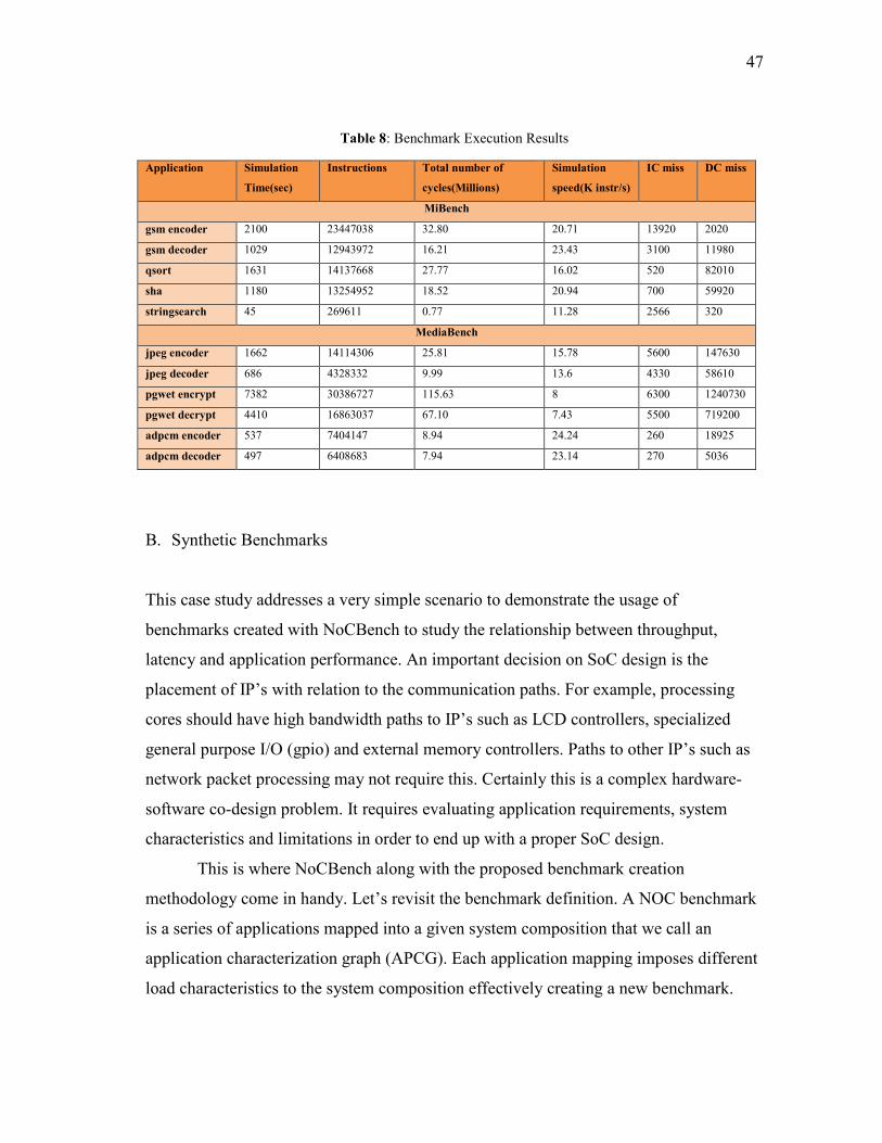
47
Table 8: Benchmark Execution Results
Application Simulation
Time(sec)
Instructions Total number of
cycles(Millions)
Simulation
speed(K instr/s)
IC miss DC miss
MiBench
gsm encoder 2100 23447038 32.80 20.71 13920 2020
gsm decoder 1029 12943972 16.21 23.43 3100 11980
qsort 1631 14137668 27.77 16.02 520 82010
sha 1180 13254952 18.52 20.94 700 59920
stringsearch 45 269611 0.77 11.28 2566 320
MediaBench
jpeg encoder 1662 14114306 25.81 15.78 5600 147630
jpeg decoder 686 4328332 9.99 13.6 4330 58610
pgwet encrypt 7382 30386727 115.63 8 6300 1240730
pgwet decrypt 4410 16863037 67.10 7.43 5500 719200
adpcm encoder 537 7404147 8.94 24.24 260 18925
adpcm decoder 497 6408683 7.94 23.14 270 5036
B. Synthetic Benchmarks
This case study addresses a very simple scenario to demonstrate the usage of
benchmarks created with NoCBench to study the relationship between throughput,
latency and application performance. An important decision on SoC design is the
placement of IP’s with relation to the communication paths. For example, processing
cores should have high bandwidth paths to IP’s such as LCD controllers, specialized
general purpose I/O (gpio) and external memory controllers. Paths to other IP’s such as
network packet processing may not require this. Certainly this is a complex hardware-
software co-design problem. It requires evaluating application requirements, system
characteristics and limitations in order to end up with a proper SoC design.
This is where NoCBench along with the proposed benchmark creation
methodology come in handy. Let’s revisit the benchmark definition. A NOC benchmark
is a series of applications mapped into a given system composition that we call an
application characterization graph (APCG). Each application mapping imposes different
load characteristics to the system composition effectively creating a new benchmark.

48
The cores could then be interconnected with different NOC architectures to make
comprehensive evaluations.
The NoCBench synthetic benchmarks can be controlled per application where
each can be run for several iterations (i.e. jobs). However, since this a simple
demonstration we only ran one job per application. The benchmarks selected was
Networking. Two topologies were chosen: 3X3 mesh and 3X3 torus. Figure 25 presents
the logical placement of the cores. Links and routers are not shown for simplicity.
Maximum Sustained transmit throughput was gathered using the same
measurement points described in Chapter IV. End-to-end latency was gathered as an
average per core. As explained in Chapter IV each packet carries a time stamp with the
time of injection and the receiving core computes the end-to-end latency by capturing
the time stamp at receive time. Therefore this average represents the aggregated end-to-
end latency to reach each core from any point in the NOC. This evaluates the congestion
on the paths of interests per core.
As Figure 26 shows torus improves average transmit throughput. On the other
hand, as shown in Figure 27 end-to-end latency does not improve much ranging from
5ns to 8µs. Also, Torus seems to improve the throughput balance on the system while it
does not for end-to-end latency. From, the characterization we know that Networking
C0 C1 C2
C3
C6
C4
C7
C5
C8
Figure 25: NoC Topology and IP Placement

49
has 5 of 9 cores carrying loads which are equally sensitive to throughput and latency.
Also 3 cores are sensitive to throughput. This is reflected in the application execution
times as shown in Figure 28. Networking applications see significant performance
improvement with the torus topology. This is due to the significant improvement in
throughput and while latency did not improve much it did not worsen. Moreover, from
the characterization we know that core 7 is latency sensitive and core 3, while sensitive
to both metrics, showed the worse performance in cL4. These are the two cores that
show improvement in latency on torus. We see this correlation in the performance
improvement.
Figure 26: Throughput Mesh vs Torus

50
Although this case study is very simple many other problems may be studied
with NoCBench. Network traffic balance is a very important problem when doing power
Figure 27: Latency Mesh vs Torus
Figure 28: Execution Time per Application (s)

51
characterization of an SoC and studying hot-spot formation on the system. As explained
in the previous chapter NoCBench includes power measurements as well as traffic
measurements. NoCBench is equipped to gather these statistics for all type of
benchmarks whether it is real applications or synthetic benchmarks.
For example, using the Networking benchmark we are able to see the traffic
balance in the routers as a function of % of flits traversed per router. The sampling rate
used was 1ms. The graphs in Figure 29 and Figure 30 present the first 10 ms of statistics.
We can see how the Torus topology significantly improves balance in the routers.
Figure 29: Flits Traversed per Router Over Time (%): Mesh

52
Figure 30: Flits Traversed per Router Over Time (%): Torus

53
CHAPTER VI
CONCLUSION & FUTURE WORK
The design of SoC’s is a complex process where application requirements are an
important factor in the decision of parameters, components and software used in the
system. Proper validation techniques are key for fast, accurate and efficient design.
Benchmarking is one important validation technique that allows for standard comparison
of distinct approaches.
This thesis addresses the lack of available platforms for creating proper
benchmarking scenarios to validate NOC design. It has presented NoCBench, a NOC-
based SoC simulator written in SystemC, as a plausible solution. NoCBench allows fast
and accurate simulation of Network on Chip based SoC designs and is capable of
simulating a full system with standard application benchmarks. Hence NoCBench
enables quick validation of design of each component of the system and overall
performance.
Synthetic applications can also be modeled based on real application execution.
These benchmarks allow faster simulation compared to real applications and create the
same communication characteristics. Different from data traces and statistical data, the
timing of transactions are not fixed. This allows for proper evaluation since
communication dependencies in space drive the communication isolating the on-chip
network as the sole component affecting traffic injection timing, thus affecting the
application performance.
Clear demonstration of the NoCBench features was addressed in Chapter V with
a series of case studies. Each respectively illustrate the ease of simulation and the
accuracy gained by simulating application execution with the NOC as well as the
benchmarking capabilities of NoCBench.
Regarding synthetic benchmarks however, improvement on applications is
needed. Better application models are necessary to improve the benchmarking scenarios.

54
Information on instructions could allow better timing simulation as well as power
modeling of the cores themselves. More robust communication dependency
specifications are needed as well as scaling of applications to address proper NOC sizes.
Processing time at the task level could be added to the communication dependencies as
well. Not to be confused with data traces, this information does not impose a specific
time when transactions occur, but how much processing time must pass after
dependency has been met for the transactions to initiate. This already is addressed by
NoCBench at the application level, with jobs and application period. Nonetheless,
reducing the granularity to the task level would enrich the overall benchmarking
scenario.

55
REFERENCES
[1] P. Guerrier and A. Greiner, "A generic architecture for on-chip packet-switched
interconnections," in Proc. of the 2000 Design, Automation and Test in Europe
Conference and Exhibition, Paris, France, 2000, pp. 250-256.
[2] P. Bhojwani and R. Mahapatra, "Core network interface architecture and latency
constrained on-chip communication," in Proc.of the 7th IEEE Intl Symposium on
Quality Electronic Devices, San Jose, California , 2006, pp. 358-363.
[3] P. Bhojwani, J.D. Lee, and R.N. Mahapatra, “SAPP: Scalable and adaptable peak
power management in NoCs,” in Proc. of the 2007 Intl. Symposium on Low
Power Electronics and Design, Portland, Oregon, 2007, pp. 340-345.
[4] L.-S. Peh and W.J. Dally, "A delay model and speculative architecture for
pipelined routers," in Proc. of the 7th International Symposium on High-
Performance Computer Architecture, Monterrey, Mexico, 2001, pp.255-266.
[5] C. Grecu, A. Ivanov, R. Pande, A. Jantsch, E. Salminen, U. Ogras, and R.
Marculescu, "Towards open network-on-chip benchmarks," in Proc of the 1st
International Symposium on Networks-on-Chip, Princeton, New Jersey , 2007,
pp.205-205.
[6] L. Chunho, M. Potkonjak, and W. H. Mangione-Smith, "MediaBench: A tool for
evaluating and synthesizing multimedia and communications systems," in Proc.
of the 30th Annual IEEE/ACM International Symposium on Microarchitecture,
Research Triangle Park, North Carolina, 1997, pp. 330-335.
[7] Guthaus A., Ringerberg J., Austin T., Mudge T., and Brown. R, 2010, MiBench,
http://www.eecs.umich.edu/mibench/
[8] U. Y. Ogras, J. Hu, and R. Marculescu, “Key research problems in NoC design:
A holistic perspective,” in Proc. of the 3rd IEEE/ACM/IFIP International
Conference on Hardware/Software Codesign and System Synthesis, Jersey City,
New Jersey, 2005, pp. 69-74.

56
[9] P.R. Panda, "SystemC: A modeling platform supporting multiple design
abstractions," in Proc. of the 14th International Symposium on System Synthesis,
Montréal, P.Q., Canada, 2001, pp. 75-80.
[10] Texas Instruments, 2010, Multicore SoC,
http://focus.ti.com/lit/ml/sprt548/sprt548.pdf
[11] Freescale, 2008, QorIQ,
http://cache.freescale.com/files/netcomm/doc/fact_sheet/QorIQ_P4080.pdf
[12] Palesi M., Patti D., and Fazzino F., 2010, Noxim, http://noxim.sourceforge.net/
[13] A. Kumar, N. Agarwal, L.-S. Peh, and N.K. Jha, "A system-level perspective for
efficient NoC design," in Proc. of the 2008 IEEE International Symposium on
Parallel and Distributed Processing, Miami, Florida, 2008, pp. 1-5.
[14] M. M. K. Martin, D. J. Sorin, B. M. Beckmann, M. R. Marty, M. Xu, A. R.
Alameldeen, K. E. Moore, M. D. Hill, and D. A. Wood, "Multifacet's general
execution-driven multiprocessor simulator (gems) toolset," SIGARCH Comput.
Archit. News, vol. 33, no. 4, pp. 92-99, 2005.
[15] P.S. Magnusson, M. Christensson, J. Eskilson, D. Forsgren, G. Hallberg, J.
Hogberg, F. Larsson, A. Moestedt and B. Werner, "Simics: A full system
simulation platform," Computer, vol.35, no.2, pp.50-58, 2002.
[16] H.-S. Wang, X. Zhu, L.-S. Peh, and S. Malik, "Orion: a power-performance
simulator for interconnection networks," in Proc. 35th Annual IEEE/ACM
International Symposium on Microarchitecture, Istanbul, Turkey, 2002, pp. 294-
305.
[17] Lavina J., 2010, Nirgam, http://nirgam.ecs.soton.ac.uk
[18] B. Towles and W. J. Dally, "Route packets, not wires: On-chip interconnection
networks," in Proc. of the 38th Annual ACM/IEEE Design Automation
Conference, Las Vegas, Nevada, 2001, pp. 684-689.

57
[19] S. Borkar, “Thousand core chips: A technology perspective.” in Proc. of the 44th
Annual Conference on Design Automation, San Diego, California, 2007, pp. 746-
749.
[20] L. Shang, L.-S. Peh, and N. K. Jha, "PowerHerd: A distributed scheme for
dynamically satisfying peak-power constraints in interconnection networks,"
IEEE Trans. on Computer-Aided Design of Integrated Circuits and Designs, vol.
25, no. 1, pp. 92-110, 2006.
[21] Y. Jin, E. J. Kim, and K. H. Yum, "Peak power control for a QoS capable on-
chip network," in Proc. of the 2005 Intl. Conf. on Parallel Processing, Oslo,
Norway, 2005, pp. 585-592.
[22] P.P. Pande, C. Grecu, A. Ivanov, R. Saleh, and G. De Micheli, "Design,
synthesis, and test of networks on chips," IEEE Design & Test of Computers, vol.
22, no.5, pp. 404-413, 2005.
[23] S. Rigo, G. Araujo, M. Bartholomeu, and R. Azevedo, "ArchC: A systemC-based
architecture description language," in Proc. of the 16th Symposium on Computer
Architecture and High Performance Computing, Foz do Iguacu, Brazil, 2004, pp.
66-73.
[24] Open core protocol specification, OCP International Partnership, 2007.
[25] G. Beltrame, L. Fossati, and D. Sciuto, “ReSP: A nonintrusive transaction-level
reflective MPSoC simulation platform for design space exploration” Trans.
Comp.-Aided Des. Integ, vol. 28, no. 12, pp 1857-1869, 2009.
[26] Motorola, 2007, Long term evolution (LTE): A technical overview,
http://www.motorola.com/staticfiles/Business/Solutions/Industry%20Solutions/S
ervice%20Providers/Wireless%20Operators/LTE/_Document/Static%20Files/68
34_MotDoc_New.pdf

58
APPENDIX A
Figure A.1: Consumer Throughput Characterization (B/s)
Figure A.2: Consumer Latency Characterization (ns)

59
Figure A.3: Networking Throughput Characterization (B/s)
Figure A.4: Networking Latency Characterization (ns)

60
APPENDIX B
This appendix provides the NoCBench user guide.
B.1 About
NoCBench is a benchmarking platform geared towards NOC benchmark creation and
NOC design space exploration.
B.2 Features
SystemC Compatible: NoCBench is designed with a SystemC Engine
Flexible NOC Topologies: NoCBench supports any type of topology from NXN Mesh
and Torus to any non-uniform topologies
ISS Plugin: NoCBench provides a straightforward interface to the on-chip network
architecture using OCP as the standard core-network interface. A model of SparcV8
from the ArchC project is already provided.
Real Benchmark: NoCBench supports popular benchmarks such as SpeC2000 ,
MediaBench and MiBench as well as many others.
Varied Library of IP’s and Component: From several Router models, including
PowerHerd models for power management study, to CNI’s, real processors, SRAM
models, dummy cores and TGFF cores supporting the modeling of synthetic
applications.
B.3 Download
The best way to download NoCBench is by using Subversion (SVN). You may do so by
running the command below (provided that SVN is installed on your system):

61
svn co https://nocbench.svn.sourceforge.net/svnroot/nocbench nocbench
Please refer to the SVN website for more information and usage information:
http://subversion.apache.org/
B.4 Installing NoCBench
Once the code is checked out using SVN follow the commands below from the directory
the download command was executed to install NoCBench:
1. cd [nocbench]
2. make
Where [nocbench] is the name of the top directory.
B.5 Running a Benchmark and The XML Configuration
NoCBench uses XML configuration scripts to input all simulator parameters. NoCBench
parses the XML configuration script, generates the NOC system and then starts the
simulator. There are two main types of simulation on NoCBench:
1) Real Benchmark Simulation and
2) TGFF Synthetic application benchmarking
Simulation type is divided into these categories since at the moment they are mutually
exclusive and the XML configuration format varies between the two.
B.5.1 Real Benchmark Simulation

62
In this user guide we use the cjpeg benchmark from MediaBench to illustrate how to run
a real application benchmark on NoCBench. To run the cjpeg benchmark you may
follow the command below:
[nocbench]/nocbench jpeg.xml
The jpeg.xml contains the simulation configurations. Below is the jpeg.xml.
<?xml version="1.0" encoding="ISO-8859-1"?> <!DOCTYPE Simulator SYSTEM "../conf/config.dtd"> <Simulator cycles="0" maxresponsetime="0" quietmode="true"> <PowerModel tgpb="10000" pgpb="8" ebuffread="76" ebuffwrite="80" ecrossbar="83" elink="6"/> <Network nvcs="3" buflen="8"> <CNI name="sparc-1-cni" type="ocp" infifolen="8" outfifolen="8" msgqlen="4" reorder="false"/> <CNI name="mem-1-cni" type="ocp" infifolen="8" outfifolen="8" msgqlen="4" reorder="false"/> <Router name="router1" type="generic" infifolen="8" outfifolen="8"/> <Link src="sparc-1-cni" dst="router1"/> <Link src="mem-1-cni" dst="router1"/> </Network> <CORE name="SPARC-1" type="sparcv8" interface="sparc-1-cni" pref_mem="MEMORY-1"/> <CORE name="MEMORY-1" type="memory" interface="mem-1-cni" addr_range="0x2000000"/> <System tick="100000.0" pagesize="4096" ptablesize="32" endian="1" sched="rr" heapsize="3145728" procsize="5242880" /> <Task cmdline="jpeg/bin/cjpeg -dct int -progressive -opt -outfile rose.jpeg jpeg/input/testimg.ppm" target="sparcv8" jobs="1"/> </Simulator>
The <Network> Section describes the NOC topology and configures the CNI and
Routers. The <CORE> sections is used to specify how many cores, what architecture or
type of core to use (i.e. SparcV8, Memory), and what CNI (or interface) to connect the
core. The <System> section configures the kernel. Some configurable parameters are
tick, page size and scheduler type (in this case Round Robin specified by “rr”). The
<Task> section specifies the benchmark to run. Note that we have given a relative
address in this example and that it is assumed the jpeg benchmark directory is in the
current directory (i.e. where the run command is executed). Also note that the <Task>

63
section provides for specifying target architecture and number of jobs for the task.
While the latter is optional the former is critical since binaries are compiled for a specific
target. The scheduler uses this information during simulation. A bigger system may be
specified by adding more Cores and/or NOC components (i.e CNI, Router). Also, as
man y tasks as the user requires can be specified.
B.5.2. Synthetic Benchmark Simulation (TGFF)
In this user guide we use a very simple 3-node synthetic benchmark to explain how to
run synthetic applications based on directed-acyclic graphs (DAG). To run the synthetic
benchmark you may run the following commad:
[nocbench]/nocbench peakTL.xml
The peakTL.xml contains the configuration parameters. A copy of it is show here.
<?xml version="1.0" encoding="ISO-8859-1"?> <!DOCTYPE Simulator SYSTEM "../../../conf/config.dtd"> <Simulator cycles="0" maxresponsetime="0" quietmode="true"> <PowerModel tgpb="10000" pgpb="8" ebuffread="76" ebuffwrite="80" ecrossbar="83" elink="6"/> <Network nvcs="3" buflen="8"> <CNI name="tgff-1-cni" type="ocp" infifolen="8" outfifolen="8" msgqlen="4" reorder="false"/> <CNI name="tgff-2-cni" type="ocp" infifolen="8" outfifolen="8" msgqlen="4" reorder="false"/> <CNI name="tgff-3-cni" type="ocp" infifolen="8" outfifolen="8" msgqlen="4" reorder="false"/> <Router name="router1" type="generic" infifolen="8" outfifolen="8"/> <Router name="router2" type="generic" infifolen="8" outfifolen="8"/> <Router name="router3" type="generic" infifolen="8" outfifolen="8"/> <Link src="tgff-1-cni" dst="router1"/> <Link src="tgff-2-cni" dst="router2"/> <Link src="tgff-3-cni" dst="router3"/> <Link src="router1" dst="router2"/> <Link src="router2" dst="router3"/> </Network> <CORE name="tgff-0" type="tgff" interface="tgff-1-cni" addr_range="0x1"/>

64
<CORE name="tgff-1" type="tgff" interface="tgff-2-cni" addr_range="0x1"/> <CORE name="tgff-2" type="tgff" interface="tgff-3-cni" addr_range="0x1"/> <System sched="tgff"/> <Task target="tgff" prefproc="tgff-0" sinks="1" datavol="5999616" appzname="appz1"/> <Task target="tgff" prefproc="tgff-1" srcs="0" sinks="2" datavol="1000448" appzname="appz1"/> <Task target="tgff" prefproc="tgff-2" srcs="1" datavol="0" appzname="appz1"/> <Appz name="appz1" period="1600000" jobs="1"/> </Simulator>
Note that the <Network> section and the <Core> section remain the same. The
difference here is that the type of the core is specified to be “tgff” instead of “sparcv8”.
Also notice that the scheduler specified is “tgff” the default scheduler provided by
NoCBench for synthetic application benchmarking.
The main difference between real benchmarks and synthetic applications is in the
<Task> specification section. In this mode, each <Task> is considered a node of a DAG.
To describe the links between one node and another the parameters srcs and sinksare
used. These parameters specify the “id” of the node it is connecting too, while datavol
specifies how much data it needs to transfer to the sinks. To know the id of each task is
easy, since NoCBench will automatically assign the id’s in the order the tasks are
specified starting with index 0. Since a NOC Benchmark is composed of a series of
applications each task (i.e. node) needs to specify to which application it belongs. The
<Appz> section is used to configure the parameters of each application.
A list of all configurable parameters is explained below. You may find this also at
[nocbench]/conf/config.dtd
<!-- Simulator is the root element and contains the entire simulation configuration. Each configuration must have a Network description and a System description. PowerModel, CORE, Task and Appz are optional and are only required in certain simulation modes.

65
Note: Current version performs only a partial validation of the configuration through DTD validation. However, to ensure successful simulation explicit checks for ill configured XML will be nice and helps avoiding unnecessary debugging. --> <!ELEMENT Simulator (PowerModel?,Network, CORE*, System, Task*, Appz*)> <!ATTLIST Simulator cycles CDATA #REQUIRED> <!-- number of cycles to run - infinite if 0 --> <!ATTLIST Simulator maxresponsetime CDATA #IMPLIED> <!-- number of cycles before reporting a possible deadlock --> <!ATTLIST Simulator quietmode CDATA #IMPLIED> <!-- false for verbose output, true otherwise --> <!ATTLIST Simulator randomflitrate CDATA #IMPLIED> <!-- true if flitrate is random over time - NOTE: not implemented in all modes --> <!ATTLIST Simulator trace CDATA #IMPLIED> <!-- tracefile name - used for power trace --> <!-- PowerModel element specifies the power model used in the router design. Optional should implmement sub-elements and provide more detail for router, cni, link etc. --> <!ELEMENT PowerModel EMPTY> <!ATTLIST PowerModel tgpb CDATA #REQUIRED> <!-- thermal time constant of the chip - in cycles --> <!ATTLIST PowerModel pgpb CDATA #REQUIRED> <!-- global power budget of the chip - in Watts --> <!ATTLIST PowerModel ebuffread CDATA #REQUIRED> <!-- energy of buffer read in one cycle - in pJoules --> <!ATTLIST PowerModel ebuffwrite CDATA #REQUIRED> <!-- energy of buffer write operation in one cycle - in pJoules --> <!ATTLIST PowerModel ecrossbar CDATA #REQUIRED> <!-- energy of sending a flit through the crossbar in one cycle - in pJoules --> <!ATTLIST PowerModel elink CDATA #REQUIRED> <!-- energy of writing a flit to the link - in pJoules --> <!-- Network element contains the description of the entire NoC. The components are as Router, CNI and Link each defined later in the document. Network must have One or more CNI, one or more Router and Zero or more link and in the given order. The CNIs are assigned ID based on the order of declaration starting from 0. --> <!ELEMENT Network (CNI+,Router+,Link*)> <!ATTLIST Network nvcs CDATA #REQUIRED> <!-- number of virtual channels used for the wormhole communication -->

66
<!ATTLIST Network buflen CDATA #REQUIRED> <!-- number of buffers in the CNIs for incoming and outgoing messages --> <!ATTLIST Network neighborhood CDATA #IMPLIED> <!-- hop distance to consider as neighrborhood in localized random traffic - deprecated --> <!-- Router - describes the parameters of the Router architecture.--> <!ELEMENT Router EMPTY> <!ATTLIST Router name ID #REQUIRED> <!-- name of the router - string, has to be unique --> <!ATTLIST Router type (generic) #REQUIRED> <!-- router type - has to be among the supported type --> <!ATTLIST Router ports CDATA #IMPLIED> <!-- number of ports in the router - DEPRECATED --> <!ATTLIST Router infifolen CDATA #REQUIRED> <!-- input fifo length in flits --> <!ATTLIST Router outfifolen CDATA #REQUIRED> <!-- output fifo length in flits, only used if output buffering is implemented --> <!ATTLIST Router x CDATA #IMPLIED> <!-- option to specify the co-ordinates for regulal topology horizontal position --> <!ATTLIST Router y CDATA #IMPLIED> <!-- same as above - vertical position --> <!ATTLIST Router N CDATA #IMPLIED> <!-- powerherd scheme spefici parameter --> <!-- CNI Element configuration. Each CNI element creates an interface to the NOC. Specifying type is required and important to match with the router it connects to. Note: Should be automatically matched in future versions. --> <!ELEMENT CNI (MMAP*)> <!ATTLIST CNI name ID #REQUIRED> <!-- name of the CNI, need to be unique, used to refer later on --> <!ATTLIST CNI type (ocp|pc) #REQUIRED> <!-- CNI type, required, specifies the CNI design type --> <!ATTLIST CNI infifolen CDATA #REQUIRED> <!-- input fifo length in flits --> <!ATTLIST CNI outfifolen CDATA #REQUIRED> <!-- output fifo length in flits --> <!ATTLIST CNI msgqlen CDATA #REQUIRED> <!-- length of the core side message queue --> <!ATTLIST CNI reorder (true|false) #REQUIRED> <!-- if false messages are not ordered --> <!ATTLIST CNI flitinjectionrate CDATA #IMPLIED> <!-- controls flit injection - limits if more, but increase if less is controlled by internal flag --> <!ATTLIST CNI firprofile CDATA #IMPLIED> <!-- allows to vary the injcetion over time format: "10 20 60 30" means at 10% simulation time FIR = 20% and so on-->

67
<!ATTLIST CNI ber CDATA #IMPLIED> <!-- bit error rate: to introduce error in the sent/received data at CNI --> <!-- MMAP Element Was used to specify memory map as visible through the current interface/CNI DEPRECATED --> <!ELEMENT MMAP EMPTY> <!ATTLIST MMAP base CDATA #REQUIRED> <!ATTLIST MMAP range CDATA #REQUIRED> <!ATTLIST MMAP target IDREF #REQUIRED> <!-- Link Defines a Link --> <!ELEMENT Link EMPTY> <!ATTLIST Link src IDREF #REQUIRED> <!-- src node - can be a router or cni: refered by the name attribute --> <!ATTLIST Link dst IDREF #REQUIRED> <!-- dst node - same as above --> <!-- Core element Contains the configuration for a CORE that will be attached to an interface. --> <!ELEMENT CORE EMPTY> <!ATTLIST CORE name ID #REQUIRED> <!-- name of the core: string has to be unique --> <!ATTLIST CORE type (dummy|sparcv8|memory|tgff) #REQUIRED> <!-- type of the core --> <!ATTLIST CORE interface IDREF #REQUIRED> <!-- name of the interface (CNI) this core connects to. Not verified --> <!ATTLIST CORE commandline CDATA #IMPLIED> <!-- commandline to execute in this core: used in context of ArchC cores --> <!ATTLIST CORE addr_range CDATA #IMPLIED> <!-- address range allocated to this core: just specifies the number of locations allocated --> <!ATTLIST CORE pref_mem IDREF #IMPLIED> <!-- name of the memory core where application should be loaded - DEPRECATED --> <!ATTLIST CORE bs CDATA #IMPLIED> <!-- This parameter has been deprecated. DO NOT USE --> <!-- Task element Specifies a Task to be run --> <!ELEMENT Task EMPTY>

68
<!ATTLIST Task cmdline CDATA #IMPLIED> <!-- contains absolute or relative path of the binary along with arguments --> <!ATTLIST Task target (dummy|sparcv8) #REQUIRED> <!-- specifies target architecture of the binary --> <!ATTLIST Task jobs CDATA #IMPLIED> <!-- # of jobs per task --> <!ATTLIST Task prefproc CDATA #IMPLIED> <!-- forces scheduler to run the task on specific core with target architecture --> <!ATTLIST Task prefmproc CDATA #IMPLIED> <!-- DEPRECATED --> <!-- System element Contains the kernel information. All attributes are optional. Values given in individual comments. Default values below. Also available @ Constants.h --> <!ELEMENT System EMPTY> <!ATTLIST System procsize CDATA #IMPLIED> <!-- This is the size of the local process space including .text, .data, .bss, heap, stack, shared mem and arguments. DEFAULTT 5MB -> 5242880 --> <!ATTLIST System ptablesize CDATA #IMPLIED> <!-- Size of page table. Indicates # of pages per table. DEFAULT 32 --> <!ATTLIST System pagesize CDATA #IMPLIED> <!-- Page Size in (B). DEFAULT 4KB -> 4096. --> <!ATTLIST System heapsize CDATA #IMPLIED> <!-- Maximum Task Heap size in local address space. Metric (B). DEFAULT 3MB -> 3145728 --> <!ATTLIST System tick CDATA #IMPLIED> <!-- Scheduerl period in (ns). Scheduler idle task will be run every tick. DEFAULT 10000 ns --> <!ATTLIST System endian CDATA #IMPLIED> <!-- Endiannes of the system. All memory and processor cores will be set to this. 1 BE, 0 LE. DEFAULT BE--> <!ATTLIST System sched CDATA #IMPLIED> <!-- Scheduler type; values: "rr". DEFAULT Round Robin -> "rr" --> <!ATTLIST System hyperperiod CDATA #IMPLIED> <!-- Hyperperiod of the tasks. Currently use as an expansion parameter for Real Time support -->
B.6 Help and Support
Please visit our forum located at SourceForge for support and more questions about how
to use NoCBench.
http://sourceforge.net/projects/nocbench/forums/forum/1026561

69
Thanks for your support and we look forward on NoCBench providing you the best
NOC simulation and benchmarking experience for your research work.

70
VITA
Name: Javier Jose Malave-Bonet
Address: Department of Electrical and Computer Engineering,
Texas A&M University,
214 Zachry Engineering Center,
TAMU 3128
College Station, Texas 77843-3128
Email Address: [email protected]
Education: B.S., Computer Engineering, University of Puerto Rico at Mayagüez,
2007
M.S., Computer Engineering, Texas A&M University, 2010