a column generation approach for the maximal covering location

1

A COLUMN GENERATION APPROACH FOR THE MAXIMAL COVERI NG

LOCATION PROBLEM

Marcos Antonio Pereira∗∗∗∗

Phone: +55 12 31232847

Fax: +55 12 31232845

[email protected]

FEG/UNESP – São Paulo State University

Engineering College – Department of Mathematics

12516-410 – Guaratinguetá, SP – Brazil

Luiz Antonio Nogueira Lorena

[email protected]

LAC/INPE – Brazilian Institute for Space Research

Associate Laboratory of Applied Mathematics and Computation

12201-970 – São José dos Campos, SP – Brazil

Edson Luiz França Senne

[email protected]

FEG/UNESP – São Paulo State University

Engineering College – Department of Mathematics

12516-410 – Guaratinguetá, SP – Brazil

∗ corresponding author

2

Abstract

This paper presents a column generation algorithm to calculate new improved lower

bounds to the solution of maximal covering location problems formulated as a p-median

problem. This reformulation results instances that are difficult for column generation

methods. The traditional column generation method is compared to the new approach,

where the reduced cost criterion employed at the column selection is modified by a

lagrangean/surrogate multiplier. The efficiency of the new approach is tested with real

data, where computational tests were conducted and showed the impact of sparsity and

degeneracy on column generation based methods.

Keywords: Facility location; Column generation; Lagrangean/surrogate relaxation.

3

1. Introduction

The logistics for distribution of products or services has been a subject of increasing

importance over the years, as part of the strategic planning of both public and private

enterprises. Decisions concerning the best configuration for the installation of facilities

in order to attend demand requests are the subject of a wide class of problems, known as

Location Problems (Drezner, 1995; Daskin, 1995). Using a graph representation,

demand nodes and candidate nodes for the installation of facilities are identified as

vertices in a network. Such problems typically occur in a discrete space, that is, a space

where the number of candidate locations and network connections is finite.

Depending on the proposed objective, facility location problems can be grouped into

two major classes. The first class deals with the minimization of the average or total

distance between clients and facilities. The classic model that represents the problems

of this class is the p-Median Problem, which seeks to select p vertices on a network

with n nodes (n > p) for the installation of facilities, such as the sum of the distances

between the demand nodes and its nearest facility is minimized. Models that minimize

the average or total distance are best suited to describe problems that occur in the

private sector, since the costs are directly related to the travel distances for the

satisfaction of the clients’ demands. Hillsman (1984) proposes some data manipulation

in order to produce new objective function cost coefficients, reducing several location

problems to a p-median problem.

The second class of facility location problems deals with the maximum distance

between any client and the facility designed to attend the associated demand. These

4

problems are known as covering problems and the maximum service distance is known

as covering distance. The Set Covering Problem (Toregas et al., 1971) determines the

minimal number of facilities which are necessary to attend all clients, for a given

covering distance. Due to formulation restrictions, this model does not consider the

individual demand of each client. In addition, the number of needed facilities can be

large, incurring high fixed installation costs. An alternative formulation considers the

installation of a limited number of facilities, even if this amount is unable to attend the

total demand. In this formulation, the condition that all clients must be served is relaxed

and the objective is changed to locate p facilities such as the most part of the existing

demand can be attended, for a given covering distance. This model corresponds to the

Maximal Covering Location Problem (MCLP). Covering models are often found in

problems of public organizations for the location of emergency services. Early

techniques for solving the MCLP tried to obtain integer solutions from the linear

relaxation equivalent of the model proposed by Church and ReVelle (1974). This

pioneer work formalizes the MCLP and presents a greedy heuristic based on vertices

exchange. Lorena and Pereira (2002) report results obtained with a lagrangean/surrogate

heuristic using a subgradient optimization method, in complement to the dissociated

lagrangean and surrogate heuristics presented in Galvão et al. (2000). Arakaki and

Lorena (2001) present a constructive genetic algorithm to solve real case instances with

up to 500 vertices.

Column generation methods has gained renewed interest for solving large scale

combinatorial problems, mainly due to the development of faster and reliable

commercial optimization software (ILOG, 2001), which allow inherently complex

problems to be solved in reasonable computing times. These methods were first applied

5

to one-dimensional cutting stock problems (Gilmore and Gomory, 1961; Gilmore and

Gomory, 1963) and, since then, have been explored in many other applications, such as

cutting stocks (Vance et al., 1994; Valério de Carvalho, 1999), vehicle routing

(Desrochers and Soumis, 1989; Desrochers et al., 1992), crew scheduling (Day and

Ryan, 1997; Souza et al., 2000a; Souza et al., 2000b) and VLSI design (Souza and

Menezes, 2000). A complete overview of the column generation theory and its

applications can be found in Lübbecke and Desrosiers (2002) and Desaulniers et al.

(2005).

The column generation technique can be applied to large linear problems when not all

variables are explicitly known or when the problem is to be solved by Dantzig-Wolfe

(1960) decomposition (in this case, the columns are the extreme points of the convex

hull of the set of feasible solutions.) The method alternates between a restricted master

problem and a column generation subproblem. By starting with a feasible columns

subset, the optimal dual solution of the restricted master problem is used to calculate the

cost coefficients of the objective function for the column generation subproblem, which

produces new columns to be added to the restricted master problem formulation. If no

productive columns (based on its reduced cost value) are obtained as solution of the

subproblem, the iterative process stops.

It is well known that the direct application of column generation methods produces

many columns that are not relevant to the final solution, slowing the solution process

convergence (tailing-off). In such case, it has been observed that the dual solutions

oscillate around the optimal dual solution, justifying the application of stabilization

methods to inhibit such behavior and, thus, accelerating the problem resolution.

6

Different techniques to prevent dual solutions to vary have been proposed, like the

Boxstep method (Marsten et al., 1975), where the optimization in the dual space is

explicitly restricted to a bounded region with the current dual solution as the central

point. The Analytic Center Cutting Plane method (du Merle et al., 1998) considers the

current analytic center of the dual function instead of the optimal dual solution, avoiding

dual values to change too dramatically. The Bundle methods (Neame, 1999; Briant et

al., 2005) define a trust region combined with penalties to prevent significant changes

between consecutive dual solutions. Senne and Lorena (2001) show the successful

application of lagrangean/surrogate relaxation to stabilize the column generation

process for p-median problems. The lagrangean/surrogate approach multiply the dual

variables by an explicit parameter, like other regularization methods (Marquardt, 1963),

but with a direct way to compute the optimal value for this parameter. Other recent

alternative methods to stabilize dual solutions have been considered in Desrosiers and

Lübbecke (2005).

This paper presents the utilization of the lagrangean/surrogate relaxation in a column

generation algorithm to calculate lower bounds to MCLP formulated as a p-median

problem. The paper is organized as follows. Section 2 presents the classical model of

the p-median problem and the corresponding formulation as a set partitioning problem

obtained through direct application of Dantzig-Wolfe decomposition to the classical

formulation. It also presents the MCLP formulated as a p-median problem. Section 3

defines the restricted master problem and presents the integration of

lagrangean/surrogate relaxation to the proposed column generation algorithm. Section 4

describes the main aspects of the algorithm implementation and in Section 5 the

7

computational results with real data are presented. Conclusions are discussed in Section

6.

2. Mathematical formulations for the p-median problem

Let G = (N, A) be a graph where N is the set of vertices, A is the set of arcs and |N| = n.

The p-median problem consists in determining p < n vertices (medians) such as the total

distance from each vertex to the nearest median is minimized. The distance matrix D =

[dij]n×n between each pair of vertices is assumed to be previously known.

The p-median problem can be formulated as the following optimization problem

(Hakimi, 1964):

PMP v(PMP) = ∑∑∈ ∈Ni Nj

ijij xdMin (1)

s. t. 1=∑∈Nj

ijx , ∀i ∈ N (2)

pxNj

jj =∑∈

(3)

jjij xx ≤ , ∀i, j ∈ N (4)

xij ∈ {0, 1}, ∀i, j ∈ N (5)

where [xij]n×n is the location-allocation matrix, with xij = 1 if vertex i is allocated to the

median j, and xij = 0, otherwise; xjj = 1 if vertex j is a median, and xjj = 0, otherwise.

8

Equation (1) corresponds to the solution cost, which is to be minimized. Constraint set

(2) and (4) guarantee that each vertex i is allocated to exactly one vertex j, which must

be a median. Constraint (3) determines the number of medians to be localized and

constraint set (5) imposes integrality to the problem variables.

An alternative presentation for PMP considers the partition of the set N into p clusters.

For this reason, p-median problems are also known as clustering problems (Vinod,

1969; Rao, 1971; Hansen and Jaumard, 1997; Fung and Mangasarian, 2000).

Swain (1974) and Garfinkel et al. (1974) proposed the application of Dantzig-Wolfe

decomposition to formulation PMP, aiming the application of column generation

techniques to solve p-median problems. Considering S = {S1, S2, …, Sm} as the set of all

subsets of N, Minoux (1987) presents the formulation of a set partition problem with

cardinality constraint to describe p-median problems, as follows:

SPP v(SPP) = ∑∈Mk

kk xcMin (6)

s. t. 1=∑∈Mk

kk xA (7)

pxMk

k =∑∈

(8)

xk ∈ {0, 1}, ∀k ∈ M (9)

where:

• M = {1, 2, ..., m} is the index set of elements of S;

• = ∑∈

∈k

k Siij

Sjk dMinc , ∀k ∈ M;

9

• Ak = [aik]n×1, with aik = 1 if i ∈ Sk; aik = 0, otherwise;

• xk = 1 if subset (cluster) Sk ∈ S belongs to the solution; xk = 0, otherwise.

Each subset Sk corresponds to a column Ak of the constraint set (7), representing a

cluster in which the median is defined as the vertex j ∈ Sk that results the smallest total

distance to all i ∈ Sk and the corresponding value of ck will be set as the cluster cost. So,

constraints (4) of PMP are implicitly considered. Constraints (2) and (3) are maintained

and updated to (7) and (8), respectively.

Assuming bi as the demand value at each vertex i ∈ N, and U as the covering distance,

Hillsman (1984) proposes new cost coefficients cij to the objective function (1) as

follows:

>≤

=Udb

Udc

iji

ij

ij if ,

if ,0 (10)

This transformation allows that methods developed to p-median problems can be

applied to solve maximal covering location problems (Lorena and Pereira, 2002).

The optimal value v(PMP) of the objective function (1) with cost coefficients calculated

as in (10) denotes the non-attended demand. The optimal value for the corresponding

MCLP is calculated as:

attended demand = ∑∈Ni

ib – v(PMP)

10

3. A stabilization method for column generation

As commented before, the solution of large scale linear problems by column generation

methods is an iterative process, starting with a feasible subset of columns and adding

new columns to a restricted master problem (RMP) at each iteration. Considering the

subset K ⊂ M = {1, 2, …, m} of all column indexes from the formulation SPP, the

corresponding RMP can be formulated as the following linear relaxation of a set

covering problem with cardinality constraint:

SCP v( SCP) = ∑∈Kk

kk xcMin (11)

s. t. 1≥∑∈Kk

kk xA (12)

pxKk

k =∑∈

(13)

xk ∈ [0, 1] ∀k ∈ K (14)

The optimal dual solutions λ ∈ nR+ and µ ∈ R, associated to constraint set (12) and

constraint (13) respectively, can be used to obtain new incoming columns to SCP and,

as presented in Senne and Lorena (2000), to calculate lower bounds by solving the

lagrangean/surrogate relaxation of problem PMP (note that hereafter cij, given by (10),

replaces dij). This relaxation can be obtained as follows.

As proposed by Glover (1968), for λ ∈ nR+ , a surrogate relaxation of (PMP) can be

defined by:

SPMP v(SPMP) = ∑∑= =

n

i

n

jijij xcMin

1 1

(15)

11

s. t. ∑∑ ∑= = =

=n

j

n

i

n

jjijj x

1 1 1

λλ (16)

and (3) – (5).

The problem SPMP can not be easily solved, as it is an integer linear problem with no

special structure to be explored. Due to this difficulty, constraint (16) in problem SPMP

is relaxed again, now in the lagrangean way for t ∈ R, and the lagrangean/surrogate

relaxation of PMP is given by:

LSPMP v(LSPMP) = ∑∑∑∈∈ ∈

+−Ni

iijNi Nj

iij txtcMin λλ )(

s. t. (3) – (5).

For any given λ ∈ nR+ , the best lagrangean/surrogate multiplier t can be obtained either

as the optimal solution of the dual of LSPMP, defined as:

D v(D) = { })(LSPMPvMaxt

,

or by a dichotomous search, since the lagrangean function l: t → v(LSPMP) is concave

and piecewise linear (Parker and Rardin, 1988).

For any t and λ, it is well known that v(LSPMP) ≤ v(SPMP) ≤ v(PMP). Setting t = 1 in

LSPMP results the usual lagrangean relaxation of PMP with multiplier λ. The optimal

value v(LSPMP) provides better lower bounds than the usual lagrangean bounds, as can

be observed from the computational results presented in this paper.

12

Let j* be the vertex defined as the median of the cluster with the smallest contribution to

v(D) which is determined as the optimal solution of the following subproblem:

CGS v(CGS) = −∑∈∈∈

Niijiij

aNjatcMinMin

ij

)(}1,0{

λ

Subproblem CGS can be easily solved by inspection, assuming each vertex j ∈ N as

median and setting aij, ∀i ∈ N, as follows:

>−

≤−=

.0 if ,0

.0 if ,1

iij

iij

ij tc

tca

λλ

Let Sj* be defined as Sj* = { i ∈ N | aij * = 1}. The corresponding column 1

*jA will be

added to SCP if:

µλ <−∑∈∈

Niijiij

aacMin

ij**

}1,0{)(

*

(17)

In effect, in order to accelerate the solution process of column generation methods,

every column 1

jA, j ∈ N, satisfying condition (17) can be added to RMP (multi-

pricing). It is easy to see that, for t ∈ [0, 1], if cij – λi > 0 then cij – tλi > 0 and the

corresponding aij = 0 in the column 1

jA is not modified by using multiplier t. On the

13

other hand, if cij – λi ≤ 0 then cij – tλi ≤ 0 or cij – tλi > 0 and in the column 1

jA some

aij = 1 can be flipped to aij = 0. A straightforward consequence is that the column cost = ∑∈∈

kk Si

ijSj

k cMinc , calculated by the lagrangean/surrogate approach, can be smaller than

the one obtained by the traditional lagrangean, for the same multipliers λi. Hence, as it

is possible to consider several values for the multiplier t (as we proceed in some

computational tests), a greater number of columns can be added to SCP in the

lagrangean/surrogate case. The effects of these aspects of the lagrangean/surrogate

approach are best shown on computational tests of section 5 and results in faster

convergence, even when a higher number of columns is added to the pool at each

iteration of the process.

4. The proposed column generation algorithm

Generally, in a column generation algorithm, the dual solutions for the RMP in early

iterations present very strong oscillatory behavior around the optimal dual solution, due

to the poor quality of the initial columns subset. Since these dual solutions are used in

the column generation subproblem, the performance of the algorithm can be

compromised.

In the proposed algorithm, dual solutions are modified by the lagrangean/surrogate

multiplier t. In this manner, at early iterations the poor dual solutions are multiplied by a

small positive value, minimizing their harmful effects. As new better columns are

obtained, this multiplier is consistently increased, converging to 1 as the process

14

converges to the optimal solution. This is a clever strategy for a stabilized column

generation process, since the proper value used to modify the dual solution depends on

the dual solution itself, and it is obtained from a simple local search. Other stabilization

approaches, such as the ones mentioned in Section 1, rely on more complex techniques

to control the dual solutions.

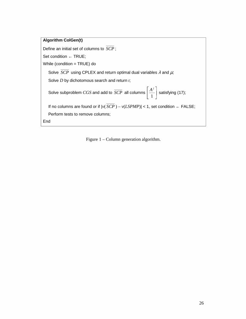
The column generation algorithm proposed in this paper can be described in Figure 1.

Note that the usual column generation algorithm is obtained simply by setting t = 1. In

this case, v(LSPMP) corresponds to the traditional lagrangean bound.

Figure 1.

The initial set of columns to SCP (starting master problem) is obtained with the

application of the subroutine depicted in Figure 2. In order to compare both the

traditional and the proposed approaches, the same initial set was used for the lagrangean

and lagrangean/surrogate cases.

Figure 2.

In order to control the problem size, a column removal subroutine was implemented

(Figure 3). This subroutine may be executed either if the number of columns in the

formulation SCP is greater than a predefined maximum value, or if is intended to keep

in the formulation only columns with reduced cost smaller than a reference average

value.

15

Figure 3.

The cost coefficients calculated in (10) does not satisfy the triangular inequality,

resulting in slow convergence of iterative lagrangean based procedures developed to

solve location problems (Schilling et al., 2000). In addition, linear program methods

applied to formulations SPP or SCP may suffer of degeneracy. This is more likely to

happen in column generation methods, as near-zero cost columns may be selected to

enter the basis in advanced iterations. For MCLP, zero cost columns are highly

desirable, as they correspond to clusters with fully attended demand, making the column

generation approach a real challenge.

Preliminary computational tests with real data MCLP instances, which are solved by the

column generation algorithm developed by Senne and Lorena (2001) for p-median

problems, presented non satisfactory convergence for both the lagrangean and

lagrangean/surrogate cases. During the solution process it was verified, in many

instances, that the lower bounds provided by LSPMP remained unchanged for many

iterations, indicating that the columns of the current master problem SCP always

produced the same optimal dual solution λ.

In order to avoid this, the algorithm ColGen(t) of Figure 1 was modified to include two

special procedures. The first was to allow all columns obtained as solution of the

column generation subproblem to be included in the RMP, even those with positive

reduced cost. This procedure, called perturbation, caused the dual solutions to change

and the lower bounds to increase again. The perturbation procedure was applied, just for

16

a single iteration, every time v(LSPMP) remained unchanged for a prefixed number of

iterations.

The second procedure is due to the inclusion of more columns into the master problem

and the behavior of the multiplier t. The lagrangean/surrogate multiplier t has zero as

the starting value and, as the ColGen(t) algorithm proceeds, its value asymptotically

converges to 1. In order to increase the algorithm’s performance at early iterations, we

considered the inclusion of columns with negative reduced cost obtained as solution of

the subproblem for the current value for multiplier t and for the values in the set

T = {0.50, 0.55, 0.60, 0.65, 0.70, 0.75, 0.80, 0.85, 0.90, 1} which are greater than the

current t, aiming the anticipation of information (columns) that would be available only

in advanced iterations. This procedure was called augmentation and applies to the

lagrangean/surrogate case only.

Computational tests showed that the application of the perturbation procedure in some

MCLP instances solved for the lagrangean/surrogate case caused the lower bound

convergence sequence to oscillate when t already converged to 1. In this case, the

algorithm produced worse values for v(LSPMP) than the previously obtained ones. For

this reason, the proposed algorithm includes a control mechanism that inhibits the

perturbation procedure, for the lagrangean/surrogate case only, if the multiplier t has

reached the value 1.

5. Computational results

17

The algorithms and subroutines presented in this paper were coded in C and compiled

with Borland C++ Builder 5, with default compiling options to create a command line

executable. Tests were conducted on a PC with Intel Pentium 4 2.6 GHz processor and

1 GB RAM, running Microsoft Windows XP Professional with Service Pack 2. The

solution of the RMPs and column generation subproblems were obtained with ILOG

CPLEX 7.5.

The instances correspond to real case data for facility location in São José dos Campos -

Brazil. They are available at http://www.lac.inpe.br/~lorena/instancias.html.

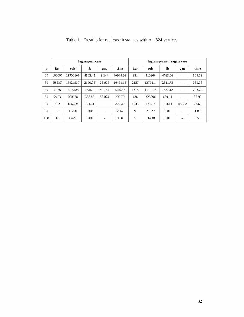
The computational results are shown in the Tables 1 to 5. These tables contain:

p: number of facilities to be located;

iter : number of performed iterations;

cols: total number of generated columns;

lb: best v(LSPMP) found;

gap: relative difference between v( SCP) and the lower bound (in %);

time: total computational time (in seconds).

Note that the values in the Tables 1 to 5 for the lagrangean case were obtained by

setting t = 1 in the algorithm ColGen(t). In any case, the perturbation procedure was

executed every time the value v(LSPMP) remained unchanged for 10 consecutive

iterations.

18

The maximum number of iterations was fixed at 100000. As new columns are obtained

and introduced in the formulation, the value v( SCP) decreases, acting as an upper

bound. The algorithm stops when the bounds converged to the same value (that is

indicated with the symbol “–” in gap column of Tables 1 to 5) or if v( SCP) <

v(LSPMP).

Table 1

Table 2

Table 3

Table 4

Table 5

As the results show, more columns were generated for the lagrangean case but it did not

implied in better bounds. The lagrangean/surrogate multiplier seems to affect drastically

the column generation subproblem, resulting in better quality columns and producing

better bounds in less computational time. The lagrangean case showed to be more

sensitive to the effects of degeneracy, as can be observed by the number of generated

columns, indicating the intense use of the perturbation procedure.

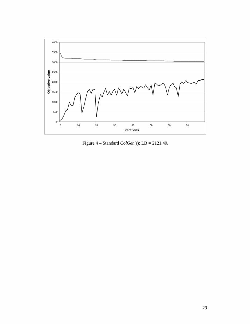
The effects of the controlled perturbation and augmentation for the lagrangean/surrogate

case can be observed in Figures 4 to 6. The graphics show the evolution of primal

19

values v( SCP) (upper portion curve) and dual values v(LSPMP) (lower portion curve)

for a MCLP instance with n = 324, p = 20 and U = 150. In Figure 4, algorithm

ColGen(t) stopped after 80 iterations (no incoming columns criterion), resulting a lower

bound of 2121.40.

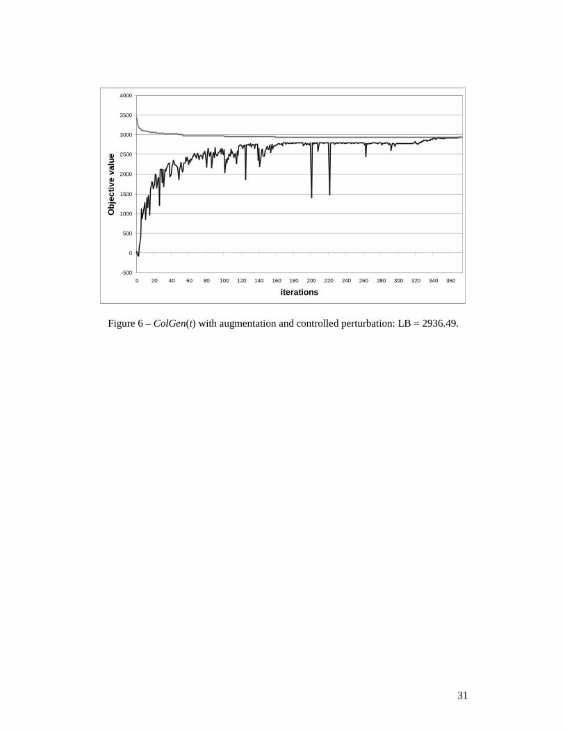
The augmentation procedure was then performed, and the execution was extended until

iteration 1972 (Figure 5), stopping after 1000 consecutive iterations with no

improvement to v(LSPMP). Figure 6 shows the evolution of the solution process with

augmentation and controlled perturbation, and convergence of the bounds after 374

iterations.

Figure 4

Figure 5

Figure 6

The smaller number of generated columns for the lagrangean/surrogate case indicates

that the use of the lagrangean/surrogate multiplier in the calculation of the cost

coefficients for the objective function of the column generation subproblem helps to

produce better quality columns. As the computational results showed, in many instances

the usual lagrangean column generation algorithm stopped only after the maximum

iteration number was reached, with poor lower bounds.

6. Conclusion

20

This paper presented a simple stabilization method for Maximal Covering Location

problems (MCLP) formulated as p-median problems and solved by a column generation

algorithm. This reformulation produced instances that are difficult to standard column

generation approaches, which result in lacks of convergence or higher oscillations in

dual solutions at early stages.

The lagrangean/surrogate stabilization is fast and straightforward, based on lagrangean

relaxation dual and reassembling other regularization methods. The best regularization

parameter is directly identified by dichotomous search. As shown in computational tests

with real instances the lagrangean/surrogate approach is faster and reliable, although

more research must be performed to shorten computational times. This will be

important if one consider the proposed approach as the core algorithm in a branch-and-

price method to produce feasible (integer) solutions to MCLP instances.

Acknowledgements: The authors acknowledge Coordenação de Aperfeiçoamento de

Pessoal de Nível Superior (CAPES) and Conselho Nacional de Desenvolvimento

Científico e Tecnológico (CNPq) for partial financial research support. Comments and

suggestions of two anonymous referees were much appreciated.

References

1. Arakaki, R.G.I., Lorena, L.A.N., 2001. A constructive genetic algorithm for the

maximal covering location problem. In: Proceedings of the 4th Metaheuristics

International Conference (MIC’2001), 16-20 jul., Porto, Portugal, 13-17.

21

2. Briant, O., Lemaréchal, C., Meurdesoif, P.H., Michel, S., Perrot, N., Vanderbeck, F.,

2005. Comparison of Bundle and Classical Column Generation, Rapport de

recherche de l'INRIA 5453, Rhone-Alpes, France.

3. Church, R.L., ReVelle, C.S., 1974. The maximal covering location problem. Papers

of the Regional Science Association 32, 101-118.

4. Dantzig, G.B., Wolfe, P., 1960. Decomposition principle for linear programs.

Operations Research 8, 101-111.

5. Daskin, M., 1995. Network and discrete location: models, algorithms and

applications. New York: Wiley Interscience, 500p.

6. Day, P.R., Ryan, D.M., 1997. Flight attendant rostering for short-haul airline

operations. Operations Research 45, 649-661.

7. Desaulniers, G., Desrosiers, J., Solomon, M.M. (Eds), 2005. Column Generation.

Berlin: Springer, 358p.

8. Desrochers, M., Desrosiers, J., Solomon, M., 1992. A new optimization algorithm

for the vehicle routing problem with time windows. Operations Research 40, 342-

354.

9. Desrochers, M., Soumis, F., 1989. A column generation approach to the urban

transit crew scheduling problem. Transportation Science 23, 1-13.

10. Desrosiers, J., Lübbecke, M.E., 2005. A primer in column generation. In: G.

Desaulniers, J. Desrosiers and M.M. Solomon (Eds.), Column Generation (GERAD

25th anniversary series), Springer Science+Business Media Inc., New York, p. 1-32.

11. Drezner, Z., (Editor) 1995. Facility location: a survey of applications and methods.

New York: Springer-Verlag, 571p.

22

12. du Merle, O., Goffin, J.L. and Vial, J.P., 1998. On Improvements to the Analytic

Centre Cutting Plane Method. Computational Optimization and Applications 11, 37-

52.

13. Fung, G., Mangasarian, O.L., 2000. Semi-supervised support vector machines for

unlabeled data classification. Optimization Methods and Software 1(15), 29-44.

14. Galvão, R.D., Espejo, L.G.A., Boffey, B., 2000. A comparison of lagrangean and

surrogate relaxations for the maximal covering location problem. European Journal

of Operational Research 124, 377-389.

15. Garfinkel, R.S., Neebe, W., Rao, M.R., 1974. An algorithm for the m-median

location problem. Transportation Science 8, 217-236.

16. Gilmore, P.C., Gomory, R.E., 1961. A linear programming approach to the cutting

stock problem. Operations Research 9, 849-859.

17. Gilmore, P.C., Gomory, R.E., 1963. A linear programming approach to the cutting

stock problem: Part II. Operations Research 11, 863-888.

18. Glover, F., 1968. Surrogate constraints, Operations Research 4, 741-749.

19. Hakimi, S. L., 1964. Optimum location of switching centers and the absolute centers

and medians of a graph. Operations Research 12, 450-459.

20. Hansen, P., Jaumard, B., 1997. Cluster analysis and mathematical programming.

Mathematical Programming 79, 191-215.

21. Hillsman, E.L., 1984. The p-median structure as a unified linear model for location-

allocation analysis. Environmental and Planning A 16, 305-318.

22. ILOG CPLEX 7.1, 2001. User´s Manual. ILOG Inc., CPLEX Division.

23. Lorena, L. A. N., Pereira, M. A., 2002. A lagrangean/surrogate heuristic for the

maximal covering location problem using Hillsman's edition. International Journal

of Industrial Engineering 9(1), 57-67.

23

24. Marquardt, D.W. 1963, An Algorithm for Least-Squares Estimation of Nonlinear

Parameters. Journal of the Society for Industrial and Applied Mathematics 11, n. 2,

p. 431–441.

25. Marsten, R.E., 1975. The use of the boxstep method in discrete optimization.

Mathematical Programming Studies 3,127-144.

26. Marsten, R.E., Hogan, W.W., Blankenship, J.W., 1975. The BOXSTEP method for

large-scale optimization. Operations Research 23, 389-405.

27. Minoux, M., 1987. A class of combinatorial problems with polynomially solvable

large scale set covering/partitioning relaxations. R.A.I.R.O. Recherche

Opérationnelle 21(2), 105-136.

28. Neame, P.J., 1999. Nonsmooth dual methods in integer programming. Ph. D.

Thesis. University of Melbourne, Melbourne, 172p.

29. Parker, R.G., Hardin, R.L., 1988. Discrete Optimization. New York: Academic

Press, 472p.

30. Rao, M.R., 1971. Cluster analysis and mathematical programming. Journal of the

American Statistical Association 66, 622-626.

31. Schilling, D.A., Rosing, K.E., ReVelle, C.S., 2000. Network distance characteristics

that affect computational effort in p-median location problems. European Journal of

Operational Research 127, 525-536.

32. Senne, E.L.F., Lorena, L.A.N., 2000. Lagrangean/surrogate heuristics for p-median

problems. In Computing Tools for Modeling, Optimization and Simulation:

Interfaces in Computer Science and Operations Research, M. Laguna and J.L.

Gonzalez-Velarde (eds.) Kluwer Academic Publishers, 115-130.

33. Senne, E.L.F., Lorena, L.A.N., 2001. Stabilizing column generation using

lagrangean/surrogate relaxation: an application to p-median location problems. In:

24

European Operations Research Conference – EURO XVIII, july 9-11, Erasmus

University, Rotterdam, The Netherlands. Available for download at:

http://www.lac.inpe.br/~lorena/ejor/EURO2001.pdf

34. Souza, C.C., Menezes, C.N., 2000. Exact solutions of rectangular partitions via

integer programming. International Journal on Computational Geometry And

Applications 10 (5), 477-522.

35. Souza, C.C., Moura, A.V., Yunes, T.H., 2000a. Solving very large crew scheduling

problems to optimality. In: Proceedings of the 14th ACM Symposium on Applied

Computing (ISBN: 1-58113-240-9), 19-21 mar. Como, Italy, 446-451.

36. Souza, C.C., Moura, A.V., Yunes, T.H., 2000b. A Hybrid Approach for Solving

Large Scale Crew Scheduling Problems. In: Workshop on Practical Aspects of

Declarative Languages (PADL'00), Boston. Lecture Notes in Computer Sciences -

Proceedings of the Second International Workshop on Practical Aspects of

Declarative Languages (PADL'00). Berlin: Springer Verlag,. v. 1753, 293-307.

37. Swain, R.W., 1974. A parametric decomposition approach for the solution of

uncapacitated location problems. Management Science 21, 955-961.

38. Toregas, C., Swain, R., ReVelle, C., Bergman, L., 1971, The location of emergency

service facilities. Operations Research 19, 1363-1373.

39. Valério de Carvalho, J.M., 1999. Exact solution of bin-packing problems using

column generation and branch-and-bound. Annals of Operations Research 86, 629-

659.

40. Vance, P.H., Barnhart, C., Johnson, E.L., Nemhauser, G.L., 1994. Solving binary

cutting stock problems by column generation and branch-and-bound. Computational

Optimization and Applications 3, 111-130.

25

41. Vinod, H.D., 1969. Integer programming and the theory of groups. Journal of the

American Statistical Association 64, 506-519.

26

Algorithm ColGen(t)

Define an initial set of columns to SCP;

Set condition ← TRUE;

While (condition = TRUE) do

Solve SCP using CPLEX and return optimal dual variables λ and µ;

Solve D by dichotomous search and return t;

Solve subproblem CGS and add to SCP all columns 1

jA satisfying (17);

If no columns are found or if |v( SCP) – v(LSPMP)| < 1, set condition ← FALSE;

Perform tests to remove columns;

End

Figure 1 – Column generation algorithm.

27

Subroutine IC

Define MaxC as the maximum number of generated columns;

Set NumC ← 0;

While (NumC < MaxC) do

Define P = {n1, ..., np} ⊂ N a random set of p vertices;

For j = 1, ..., p do

Sj ← {nj} ∪ {q ∈ N – P | jqnd = }{min qt

Ptd

∈};

cj ← ∑∈∈j

j Siit

StdMin ;

For i = 1, ..., n do

If i ∈ Sj, set aij ← 1;

If i ∉ Sj, set aij ← 0;

Add column 1

jA to the initial set of columns;

NumC ← NumC + p;

End

Figure 2 – Subroutine for the initial set of columns.

28

Subroutine CR

Define TotC as the number of columns in SCP;

Define RC as the average reduced cost of the initial set of columns;

Obtain rcj, j = 1, ..., TotC, the reduced cost of every column j in SCP;

For j = 1, ..., TotC do

If rcj > RC then remove column j of SCP;

End

Figure 3 – Column removal subroutine.

29

0

500

1000

1500

2000

2500

3000

3500

4000

0 10 20 30 40 50 60 70

iterations

Ob

ject

ive

valu

e

Figure 4 – Standard ColGen(t): LB = 2121.40.

30

-500

0

500

1000

1500

2000

2500

3000

3500

4000

0 100 200 300 400 500 600 700 800 900 1000 1100 1200 1300 1400 1500 1600 1700 1800 1900

iterations

Ob

ject

ive

valu

e

Figure 5 – ColGen(t) with augmentation: LB = 2862.21.

31

-500

0

500

1000

1500

2000

2500

3000

3500

4000

0 20 40 60 80 100 120 140 160 180 200 220 240 260 280 300 320 340 360

iterations

Ob

ject

ive

valu

e

Figure 6 – ColGen(t) with augmentation and controlled perturbation: LB = 2936.49.

32

Table 1 – Results for real case instances with n = 324 vertices.

lagrangean case lagramgean/surrogate case

p iter cols lb gap time iter cols lb gap time

20 100000 11702106 4522.45 3.244 40944.96 881 510866 4763.06 – 523.23

30 59937 13421937 2160.09 29.675 16451.18 2257 1376214 2911.73 – 530.38

40 7478 1913483 1075.44 40.152 1219.45 1313 1114176 1537.18 – 292.24

50 2423 700628 386.53 58.024 299.70 438 326096 689.11 – 83.92

60 952 156259 124.31 – 222.30 1043 176719 108.81 18.692 74.66

80 33 11290 0.00 – 2.14 9 27627 0.00 – 1.81

108 16 6429 0.00 – 0.58 5 16238 0.00 – 0.53

33




30 100000 34654329 2826.46 42.107 55877.57 10441 7862281 4499.20 3.512 3393.48

40 100000 30366135 1977.76 41.166 28147.48 3146 3885112 2816.95 – 1285.91

50 26872 9101114 683.55 69.954 6364.61 3453 3512811 1789.38 – 1133.55

60 6189 2368197 –725.18 > 100 1122.58 1837 1918008 962.86 – 372.21

70 2170 830359 –610.41 > 100 312.17 1222 1897366 255.35 20.792 223.74

80 292 56664 41.06 – 28.05 1039 87151 32.05 30.336 31.64

100 32 12892 0.00 – 2.38 8 27883 0.00 – 1.62

134 15 7120 0.00 – 0.62 5 21216 0.00 – 0.59

34




40 100000 47947348 2942.82 55.219 87822.27 10797 21422705 5382.43 – 11403.01

50 100000 49810865 779.87 85.513 63239.42 29107 29005863 4168.67 9.048 8032.36

60 100000 48017859 640.88 85.428 40509.12 24108 28507334 3379.67 3.692 6826.83

70 100000 46476364 649.12 81.682 29953.01 668 2027369 1854.00 – 597.89

80 52658 25102301 –260.48 > 100 12270.24 8526 10943885 1792.27 – 1824.89

100 9618 4703855 –1077.10 > 100 2420.87 108 403308 433.99 – 74.89

130 336 130206 0.36 – 46.19 20 95257 6.83 – 7.22

167 43 22010 0.00 – 4.40 7 35617 0.00 – 1.84

35




70 100000 70801933 –8569.14 > 100 182079.69 9467 37654385 3262.17 – 23566.19

80 100000 70801933 –6273.93 > 100 127565.43 7353 28081728 2651.88 – 13826.58

90 100000 70796775 –4943.89 > 100 84151.88 9949 30628953 2305.90 – 10563.38

100 100000 70719646 –3148.53 > 100 52267.47 2358 10326618 1446.75 – 3222.66

120 16382 11582316 –3.00 > 100 38174.01 52 383893 272.47 – 155.55

140 3198 2199458 –877.93 > 100 3856.92 164 1053089 139.61 – 185.02

180 95 57986 3.01 – 18.62 243 97573 0.30 – 21.18

236 25 18105 0.00 – 2.50 7 45613 0.00 – 2.43

36




80 84679 69268588 –3.00 > 100 206442.80 29947 130865821 4173.99 25.059 100206.88

90 100000 81801981 –15780.4 > 100 178731.16 8084 40231415 2901.62 – 27721.61

100 100000 81801981 –11254.1 > 100 131980.80 4948 24244186 2411.37 32.192 16630.18

120 100000 81535844 –3117.13 > 100 46365.92 334 2797745 820.88 – 1597.38

140 21744 17627162 –2602.10 > 100 6055.78 397 2665881 509.47 – 716.29

160 6845 5599300 –9.00 > 100 2289.91 197 1352662 176.26 – 384.90

200 418 295776 6.13 – 101.070 1070 115052 8.02 65.228 103.55

273 29 23892 0.00 – 4.48 8 53002 0.00 – 3.26

37

Figure 1 – Column generation algorithm.

Figure 2 – Subroutine for the initial set of columns.

Figure 3 – Column removal subroutine.

Figure 4 – Standard ColGen(t): LB = 2121.40.

Figure 5 – ColGen(t) with augmentation: LB = 2862.21.

Figure 6 – ColGen(t) with augmentation and controlled perturbation: LB = 2936.49.

38






a column generation approach for the maximal covering location

Documents