a genetic algorithm approach for the type ii assembly line … · a genetic algorithm approach for...

A Genetic Algorithm Approach for the Type II AssemblyLine Balancing Problem

Pedro Maria de Sousa Araújo Ribeiro da Costa

Thesis to obtain the Master of Science Degree in

Mechanical Engineering

Supervisors: Prof. Carlos Baptista CardeiraProf. Paulo Miguel Nogueira Peças

Examination Committee

Chairperson: Prof. João Rogério Caldas PintoSupervisor: Prof. Carlos Baptista Cardeira

Member of the Committee: Prof. João Miguel da Costa Sousa

June 2016

Acknowledgments

I would like to thank my supervisors, Professor Carlos Cardeira and Professor Paulo Pecas, for all the

help and motivation given during the elaboration of this work. I would also like to thank Professor Rodrigo

Oliveira for all the attention and support given.

I would like to extend my sincere gratitude to Doutor Joao Pedro Tavares for all the advices and

support, when they was most needed.

I dedicate this work to my parents, siblings and Mafalda and thank them for all their love and support

throughout my course.

iii

Abstract

The presence of human operators in assembly lines is often preferred to automation systems, due to

its flexibility and capacity to deal with complex tasks. However, there is a significant dispersion of com-

pletion times for each worker, and also a large heterogeneity among workers. The traditional metrics

used to evaluate the performance of an assembly line, e.g. the smoothness of the workload, are overop-

timistic disregarding starving and blocking phenomena, resultant from the stochasticity of the workers.

In this thesis a two stage genetic algorithm approach is presented to solve the Assembly Line Balancing

Problem Type II, with stochastic heterogeneous task times and buffers between workstations. A discrete

event simulator is used to compute the objective function of each individual, evaluating simultaneously

the effect of the buffer and worker allocation on the cycle time of the line, thus allowing to take into

account the mentioned effect of the stochastic workforce. A suitable chromosomal representation allows

the algorithm to iterate efficiently the possible solutions, by varying simultaneously task sequence and

assignment to workstations, in one stage, and workers and buffer allocation in the other. The approach

is tested on a set of benchmarking problems, which were suitably extended to analyze its performance

in the presence of stochastic and heterogeneous workers. Concluding that this method is capable of

efficiently searching a wide universe of solutions.

Keywords: Assembly Line Balancing Problem; Buffer Allocation Problem; Stochastic Task Times;

Heterogeneous Workers; Genetic Algorithms; Discrete Event Simulation.

Resumo

A presenca de operadores humanos em linhas de producao apresenta-se, muitas vezes, como uma

solucao mais eficiente do que sistemas automaticos, devido a flexibilidade e capacidade de lidar com

problemas complexos que lhe sao inerentes. No entanto, verifica-se uma dispersao significativa nos

tempos de operacao de cada trabalhador, bem como uma grande heterogeneidade entre trabalhadores.

As metricas tradicionalmente utilizadas para avaliar a performance de uma linha de producao, e.g. o

equilıbrio das cargas laborais, sao demasiado otimistas, pois nao consideram paragens que ocorrem

devido ao comportamento estocastico dos trabalhadores, como bloqueamentos ou falta de pecas para

produzir. Nesta tese e proposta uma abordagem com duas fases baseada em algoritmos geneticos,

para equilibrar linhas de producao com um numero predefinido de estacoes de trabalho, buffers, tra-

balhadores heterogeneos e tempos estocasticos. Um simulador de eventos discretos e usado para

calcular a funcao de custo para cada indivıduo, considerando simultaneamente o efeito da alocacao

de buffers e de trabalhadores, permitindo assim ter em consideracao as paragens mencionadas. Uma

representacao cromossomica adequada ao problema permite que o algoritmo proposto itere eficiente-

mente as varias solucoes possıveis, atraves de reorganizacoes sucessivas da sequencia de tarefas e

da sua alocacao a estacoes de trabalho, na primeira fase, e de reconfiguracoes tanto dos buffers como

dos trabalhadores, na segunda fase. A abordagem e testada em diversos cenarios de afericao, ade-

quadamente expandidos para aferir o efeito de trabalhadores heterogeneos numa linha de producao.

Concluindo-se que este metodo e capaz de procurar eficientemente solucoes num amplo universo.

Palavras Chave: Sistemas de Montagem; Alocacao de Buffers; Tempos de operacao Estocasticos;

Trabalhadores Heterogeneos; Algoritmos Geneticos; Simulacao de Eventos Discretos.

iii

Contents

List of Tables . . . . . . . . . . . . . . . . . . . . . . . . . . . . . . . . . . . . . . . . . . . . . . vii

List of Figures . . . . . . . . . . . . . . . . . . . . . . . . . . . . . . . . . . . . . . . . . . . . . ix

Nomenclature . . . . . . . . . . . . . . . . . . . . . . . . . . . . . . . . . . . . . . . . . . . . . . xi

1 Introduction 1

1.1 Objectives and Contributions . . . . . . . . . . . . . . . . . . . . . . . . . . . . . . . . . . 2

1.2 Thesis Outline . . . . . . . . . . . . . . . . . . . . . . . . . . . . . . . . . . . . . . . . . . 2

2 Background in Balancing Line, Modeling and Metaheuristics 5

2.1 Assembly Line Balancing Problem . . . . . . . . . . . . . . . . . . . . . . . . . . . . . . . 5

2.2 Buffer Allocation Problem . . . . . . . . . . . . . . . . . . . . . . . . . . . . . . . . . . . . 7

2.3 Discrete Event Simulation . . . . . . . . . . . . . . . . . . . . . . . . . . . . . . . . . . . . 8

2.4 Stochastic Times and Heterogeneous Workers . . . . . . . . . . . . . . . . . . . . . . . . 10

2.4.1 Heterogeneous Workers . . . . . . . . . . . . . . . . . . . . . . . . . . . . . . . . . 10

2.5 Optimization with metaheuristics . . . . . . . . . . . . . . . . . . . . . . . . . . . . . . . . 12

3 Genetic Algorithm Implementation 15

3.1 The Assembly Line Balancing Problem . . . . . . . . . . . . . . . . . . . . . . . . . . . . . 16

3.2 Stochastic Workers . . . . . . . . . . . . . . . . . . . . . . . . . . . . . . . . . . . . . . . . 20

3.3 Discrete Event Simulator . . . . . . . . . . . . . . . . . . . . . . . . . . . . . . . . . . . . . 21

3.4 Genetic Algorithm . . . . . . . . . . . . . . . . . . . . . . . . . . . . . . . . . . . . . . . . 24

3.4.1 The Initial Population . . . . . . . . . . . . . . . . . . . . . . . . . . . . . . . . . . . 24

3.4.2 Fitness Function . . . . . . . . . . . . . . . . . . . . . . . . . . . . . . . . . . . . . 27

3.4.3 The Crossover Operator . . . . . . . . . . . . . . . . . . . . . . . . . . . . . . . . . 29

3.4.4 Mutation Operator . . . . . . . . . . . . . . . . . . . . . . . . . . . . . . . . . . . . 31

3.4.5 Stopping Criteria . . . . . . . . . . . . . . . . . . . . . . . . . . . . . . . . . . . . . 34

3.4.6 Best Solution . . . . . . . . . . . . . . . . . . . . . . . . . . . . . . . . . . . . . . . 34

3.4.7 Different Approaches Implementation . . . . . . . . . . . . . . . . . . . . . . . . . 34

4 Results Validation on Benchmarking Lines 37

4.1 Benchmarking Lines . . . . . . . . . . . . . . . . . . . . . . . . . . . . . . . . . . . . . . . 38

4.1.1 Assembly Lines . . . . . . . . . . . . . . . . . . . . . . . . . . . . . . . . . . . . . . 38

v

4.1.2 Presentation of the Layouts . . . . . . . . . . . . . . . . . . . . . . . . . . . . . . . 39

4.2 Discrete Event Simulator Testing . . . . . . . . . . . . . . . . . . . . . . . . . . . . . . . . 39

4.3 Compare Optimization Methods . . . . . . . . . . . . . . . . . . . . . . . . . . . . . . . . . 41

4.3.1 One Stage Approach . . . . . . . . . . . . . . . . . . . . . . . . . . . . . . . . . . 42

4.3.2 Two Stages Approach . . . . . . . . . . . . . . . . . . . . . . . . . . . . . . . . . . 43

4.4 Experiments . . . . . . . . . . . . . . . . . . . . . . . . . . . . . . . . . . . . . . . . . . . 45

4.4.1 First Stage . . . . . . . . . . . . . . . . . . . . . . . . . . . . . . . . . . . . . . . . 47

4.4.2 Second Stage . . . . . . . . . . . . . . . . . . . . . . . . . . . . . . . . . . . . . . 48

5 Conclusions 65

5.1 Future Work . . . . . . . . . . . . . . . . . . . . . . . . . . . . . . . . . . . . . . . . . . . . 66

Bibliography 69

A Precedence Graphs 75

B SBU graphs 77

B.1 Experiment 2 . . . . . . . . . . . . . . . . . . . . . . . . . . . . . . . . . . . . . . . . . . . 77

B.1.1 Layout 1 . . . . . . . . . . . . . . . . . . . . . . . . . . . . . . . . . . . . . . . . . . 77

B.1.2 Layout 2 . . . . . . . . . . . . . . . . . . . . . . . . . . . . . . . . . . . . . . . . . . 78

B.1.3 Layout 3 . . . . . . . . . . . . . . . . . . . . . . . . . . . . . . . . . . . . . . . . . . 78

B.2 Experiment 3 . . . . . . . . . . . . . . . . . . . . . . . . . . . . . . . . . . . . . . . . . . . 79

B.2.1 Layout 1 . . . . . . . . . . . . . . . . . . . . . . . . . . . . . . . . . . . . . . . . . . 79

B.2.2 Layout 2 . . . . . . . . . . . . . . . . . . . . . . . . . . . . . . . . . . . . . . . . . . 79

B.2.3 Layout 3 . . . . . . . . . . . . . . . . . . . . . . . . . . . . . . . . . . . . . . . . . . 80

vi

List of Tables

2.1 Triangular distributions proposed by [21]. . . . . . . . . . . . . . . . . . . . . . . . . . . . 12

3.1 The multipliers applied to each type of operator. . . . . . . . . . . . . . . . . . . . . . . . . 21

4.1 Optimal configuration without buffers or stochastic task times for Jackson line. . . . . . . . 38

4.2 Optimal configuration without buffers or stochastic task times for Mitchell line. . . . . . . . 38

4.3 Optimal configuration without buffers or stochastic task times for Gunther line. . . . . . . . 39

4.4 Information of lines to be used. . . . . . . . . . . . . . . . . . . . . . . . . . . . . . . . . . 39

4.5 Information about the simulation time for each line. . . . . . . . . . . . . . . . . . . . . . . 41

4.6 Test conditions. . . . . . . . . . . . . . . . . . . . . . . . . . . . . . . . . . . . . . . . . . . 42

4.7 Final Solution obtained with OSA. . . . . . . . . . . . . . . . . . . . . . . . . . . . . . . . 43

4.8 Configuration obtained for Jackson line with OSA. . . . . . . . . . . . . . . . . . . . . . . 43

4.9 Test conditions. . . . . . . . . . . . . . . . . . . . . . . . . . . . . . . . . . . . . . . . . . . 43

4.10 Test conditions. . . . . . . . . . . . . . . . . . . . . . . . . . . . . . . . . . . . . . . . . . . 44

4.11 Final Solution obtained with TSA. . . . . . . . . . . . . . . . . . . . . . . . . . . . . . . . . 45

4.12 Results of Stg1 with Jackson Line. . . . . . . . . . . . . . . . . . . . . . . . . . . . . . . . 47

4.13 Results of Stg1 with Mitchell Line. . . . . . . . . . . . . . . . . . . . . . . . . . . . . . . . 48

4.14 Results of Stg1 with Gunther Line. . . . . . . . . . . . . . . . . . . . . . . . . . . . . . . . 48

4.15 Test conditions for Experiment 1. . . . . . . . . . . . . . . . . . . . . . . . . . . . . . . . . 49

4.16 Amplitude of CT Variation, Experiment 1. . . . . . . . . . . . . . . . . . . . . . . . . . . . 50

4.17 Final Solution with maximal buffer initial capacity value set to 1000 units, Experiment 1. . 52

4.18 Final Solution with maximal buffer initial capacity value set to 10 units, Experiment 1. . . . 54

4.19 Evaluation of variation of SBU throughout Experiment 1. . . . . . . . . . . . . . . . . . . . 55









vii



viii

List of Figures

2.1 Example of a Precedence Graph . . . . . . . . . . . . . . . . . . . . . . . . . . . . . . . . 6

2.2 Mapping of different workers. Figure taken from [21] . . . . . . . . . . . . . . . . . . . . . 11

3.1 Precedence constrains of Jackson line. . . . . . . . . . . . . . . . . . . . . . . . . . . . . 17

3.2 First iteration of the Layer Method. . . . . . . . . . . . . . . . . . . . . . . . . . . . . . . . 18

3.3 Updating of the Precedence Constrain table. . . . . . . . . . . . . . . . . . . . . . . . . . 19

3.4 Example of a 2 WS SAL, generated by the ModelBuilder rapid . . . . . . . . . . . . . . . 23

3.5 Flowchart of GA . . . . . . . . . . . . . . . . . . . . . . . . . . . . . . . . . . . . . . . . . 24

3.6 Example of Crossover process for the Task Sequence Chromosome. . . . . . . . . . . . . 29

3.7 Example of Crossover process for the WS Sequence Chromosome. . . . . . . . . . . . . 30

3.8 Example of Crossover process for the Worker Type Sequence Chromosome. . . . . . . . 31

3.9 Example of successful Mutation process for the Task Sequence Chromosome. . . . . . . 32

3.10 Example of unsuccessful Mutation process for the Task Sequence Chromosome. . . . . . 32

3.11 Example of Mutation process for the WS Sequence Chromosome. . . . . . . . . . . . . . 33

3.12 Example of Mutation process for the Worker Type Sequence Chromosome. . . . . . . . . 33

4.1 BCT (blue) vs LWSCT (red) . . . . . . . . . . . . . . . . . . . . . . . . . . . . . . . . . . . 40

4.2 SBU descent for Layout 1, Experiment 1. . . . . . . . . . . . . . . . . . . . . . . . . . . . 50



4.5 Worker Position, Experiment 1 . . . . . . . . . . . . . . . . . . . . . . . . . . . . . . . . . 53



A.1 Precedence Graph of line: Jackson. . . . . . . . . . . . . . . . . . . . . . . . . . . . . . . 75

A.2 Precedence Graph of line: Mitchell. . . . . . . . . . . . . . . . . . . . . . . . . . . . . . . . 75

A.3 Precedence Graph of line: Gunther. . . . . . . . . . . . . . . . . . . . . . . . . . . . . . . 76

B.1 SBU descent for Layout 1, Experiment 2. . . . . . . . . . . . . . . . . . . . . . . . . . . . 77




ix



x

Notation

• AGOS - Average nubmer of Generations until the Optimal Solution

• AL - Assembly Line

• ALBP - Assembly Line Balancing Problem

• ALWSBP - Assembly Line Worker Allocation Balancing Problem

• ATG - Average Time per Generation

• AV - Amplitude of Variation of SBU

• BAP - Buffer Allocation Problem

• BCT - Basic Cycle Time

• BID - Best Individual Diversification

• BII - Best Individual Intensification

• CT - Cycle Time

• DES - Discrete Event Simulator

• DS - Direct successor method

• GA - Genetic Algorithm

• IPD - Initial Population Diversification

• KPI - Key Performance Indicators

• LM - Layor Method

• LWSCT - Last Workstation Cycle Time

• MV - Mean Value of SBU

• NPP - Number of Parts Produced during the simulation

• OSA - One Stage Approach

• ROS - Runs that achived the Optimal Solution

• RSS - Runs that achived a Suboptimal Solution

• SBU - Sum of Buffer Units

• SC - Stopping Criteria

• TSA - Two Stages Approach

• WIP - Work In Process

• WS - Workstation

xi

Chapter 1

Introduction

The way researchers regard the presence of human operators in an assembly line has evolved con-

siderably since it was introduced by Henry Ford in the beginning of the twentieth century. Back then,

worker behaviour was compared to that of a machine, able to work at the same rate during the whole

shift. Naturally, this philosophy generated a very harsh working environment.

With the introduction of robotic solutions, and overall evolution of automatic assembly lines, human

operators could be removed from the most monotonous and stressful workplaces. But in many high

complexity jobs, human operators are still often preferred to automation system, because they often are

the most efficient solution, [25].

In a well-balanced assembly line, the intrinsic heterogeneous and stochastic behaviour of workers

causes congestions, which reflect in an increased overall assembly line cycle time and output variability,

[12]. To minimize this effect and allow accomplishing a target output rate and variability, several solutions

can be tested, namely the use of buffers and the distribution of the workforce. These strategies contribute

to solve the performance dispersion problems regarding the human operators, but they came with a

price, e.g. the increase of Work In Progress (WIP) and the overall cost, amongst others.

Therefore, balancing an unpaced asynchronous assembly line with buffers and heterogeneous work-

ers requires firstly the correct allocation of tasks to workstations, which constitutes the basis for the As-

sembly Line Balancing Problem, introduced by Salverson in [43]. Secondly, the optimization of the line

implicates a good solution for the mentioned strategies: the allocation of buffers, and of workers among

workstations.

The aim of this thesis is to provide an optimization algorithm capable of optimizing assembly lines

under the mentioned conditions, regarding the minimization of the cycle time and of the overall buffer

capacity. Due to the strong relation between the three problems:i) assembly line balancing problem, ii)

buffer allocation problem and iii) the heterogeneous workforce problem, it is desirable to solve all three

simultaneously, since even slight changes in the workload distribution can lead to a more efficient buffer

allocation, thus improving the system’s performance, [12].

However, that problem is proven to be too complex to solve in a practical time frame for most ap-

plications, as well as very sensitive to local minima, due to the large amount of different configurations

1

that have to be considered. To overcome that difficulty a two stages approach is proposed, which starts

by allocating the tasks among the workstations in a specific sequence, and when that process is com-

pleted, the different workers are distributed throughout the workstations, and the capacity of the buffers

between them is adjusted.

Both the assembly line balancing problem and the buffer allocation problem are NP-hard, fact which

associated with the size of the problems justifies the use of metaheuristics algorithms. Therefore, both

the stages of the approach are based on genetic algorithms. Discrete event simulation is used to evalu-

ate the fitness of the individuals. Otherwise, the congestion caused by the deviations in the task times,

would not be suitable reflected on the evaluation of the individuals.

1.1 Objectives and Contributions

In this thesis, a Two Stages Approach (TSA) is proposed to balance unpaced asynchronous assembly

lines with different lengths and task times and minimize the size of buffers placed between each work-

station, by searching for the best distribution of tasks among workstations, as well as the best allocation

of buffers and workers. In the first stage, the task sequence and allocation problem is solved, and in

the second the buffers and workers are simultaneously allocated. Both stages use genetic algorithm to

minimize a cost function, which in the first stage is analytical, and in the second is based on simulation.

To implement the mentioned algorithm a communication procedure between the genetic algorithm

and the Discrete Event Simulator was created, which constitutes a major step for future work in combin-

ing these two techniques.

Another contribution of this thesis, is the chromosomic classification of each type of worker by means

of a chromosome named Worker Type, which uses a numeric indexing to allocate the various workers

to the workstations.

1.2 Thesis Outline

• Chapter 1 - The first chapter presents the introduction of this thesis. A small text on the assembly

line balancing problems, buffer allocation problems and heterogeneous workforces is presented,

followed by the objective of this thesis.

• Chapter 2- The state of the art regarding the concepts used in the elaboration of the problem

is presented: assembly line balancing problems, buffer allocation problems and heterogeneous

workforces is presented. As well as that of the methods used to build the algorithm: discrete event

simulation and line balancing with metaheuristics.

• Chapter 3- The implementation of each concept to build the algorithm developed in this thesis is

explained.

• Chapter 4- The proposed algorithm is tested under a variety of scenarios, to assess its perfor-

mance regarding the diversification and the intensification, which are the capacity to explore a

2

wide universe of solutions efficiently, and that to find optimal solutions, respectively.

• Chapter 5- In the final chapter conclusions on the results obtained are made, as well as some

discussion about future work.

3

Chapter 2

Background in Balancing Line,

Modeling and Metaheuristics

In this chapter each concept used in the thesis is addressed by introducing the problem and present-

ing the state of the art regarding that specific area. The chapter is divided in five sections, the first

three consider the problem’s environment: an Assembly Line Balancing Problem, with buffers that have

to be suitably allocated (Buffer Allocation Problem) and Stochastic Workers with heterogeneous perfor-

mances, which have to be allocated to each workstation. The last two sections address concepts related

with the tools used to approach the problem, namely Discrete Event Simulation, and metaheuristic opti-

mization algorithms.

2.1 Assembly Line Balancing Problem

The concept of manufacturing assembly line was first introduced by Henry Ford in the begging of the

19th century. It was proposed as a highly efficient way of producing a particular good, the Ford Model-T.

Its first mathematical formulation was proposed by Salverson in [43] in the mid-fifties, who named it

the Assembly Line Balancing Problem (ALBP), and, since those early times, several developments took

place, introducing new layouts and constrains.

To comprehend the concept of ALBP firstly it is important to understand what is and how an As-

sembly Line (AL) operates. Accordingly to Scholl and Becker in [45], an AL can be defined as a set of

workstations (WS) k = 1, ...,K, arranged in a linear layout, each connected to the next via a material

handling device, responsible for moving the part from one WS to the next, e.g. a conveyor belt. A WS is

classified as any point of the line where a task (or several tasks) is performed repeatedly.

The workpieces are fed to the first WS by a mechanical system or operator, then, either a material

handling system or the operators themselves move the product downstream, from one WS to the next,

as the respective tasks are completed. After the last WS, the product is extracted from the line, also by

a mechanical system or operator. Therefore AL are considered flow oriented production systems.

The process of manufacturing a product is divided into a set of elementary and indivisible operations,

5

labeled Tasks V = 1, ..., N , which are distributed throughout the several WS that constitute the line. A

task can be executed by machinery, robots and/or human operators, and require special equipment to

be performed. The time necessary to perform the jth task is tj .

The set of tasks assigned to a given WS k, is called the station load, Sk, and considering that no

sequence-dependent setup times are involved, summing the times each task takes to be made, results

on the station time, given by t(Sk) =∑

j∈Sktj .

Generally the sequence in which the tasks are made is constrained , i.e. there are precedence

relations among some of the tasks that impose a partial ordering, thus stating which task has to be

completed before others. These constrains can be organized in a precedence graph, which is composed

by weighted nodes that represent each task (value inside the circle), as well as it’s task time (value

outside the circle), and directional arcs, that indicate the precedence constrains. Figure 2.1 shows an

example of a precedence graph taken from [9], with N = 10 tasks whose times range from 1 to 10 time

units.

Figure 2.1: Example of a Precedence Graph

There are many examples of task related constrains, [41], here two that have been mentioned are

exemplified: the worker related constrains, which occur when an operator cannot perform a certain task

(this matter will be resumed further down), and the already mentioned sequence-dependent setup times,

which have been considered in several cases, like [3], [23], [47], [48] and [63] among others.

Another very important concept is that of Cycle Time (CT), that corresponds to the maximum or

average time available for work cycle, [9], i.e. the pace of the line. There are two basic ways to set

the CT of an AL, which depend on the system that transfers the parts from one WS to the next. If a

conveyor system moves all the parts at the same time, transferring them throughout the several WS,

the line is Paced, on the other hand, if the transfer of the parts is made by each operator, when the

corresponding operation is finished, the line is Unpaced, meaning that the slowest WS, i.e. the one with

highest station time, sets the pace for the whole line - a WS in this situation is called a Bottleneck. Within

the definition of unpaced lines two scenarios can arise: the WSs can all transfer the workpiece down

the line simultaneously, or that decision is made by each WS individually. In the first case the line is

synchronous and in the second it is asynchronous.

The basic formulation of the ALBP is the Simple Assembly Line Balancing Problem (SALBP), pro-

posed by Baybars in [8], which consists of an AL with a serial layout and a certain number of WS,

where a single product is assembled. All the tasks are considered to be deterministic, and no sequence-

dependent setup times are taken into account. Also, all WS are equally equipped regarding machines

and workers. Depending on the objective of the optimization, there are, at least, two versions of this

6

problem: if the goal is to minimize the required number of WS to achieve a given CT, the problem is

named SALBP-Type 1; if, on the other hand, the number of WS is fixed, and the objective is the mini-

mization of the cycle time, by distributing the tasks among the existent WS, the problem is addressed as

SALBP-Type 2, which is the dual of Type-1.

Intermediate storage units can be placed between each WS, in order to hold a number of prod-

ucts while these wait to be admitted by the following WS. To the mentioned storage units researchers

call Buffers (B), and to the products that are stored there call Work In Progress (WIP). The capacity

and number of buffers in a line is an optimization problem called Buffer Allocation Problem, which is

addressed in section 2.2 .

This solution is especially useful in an Asynchronous AL, due to the different times the several WS

take to perform all the tasks, which generate starvation and blocking events. A starvation event takes

place between two WS, when the one placed upstream is slower than the one downstream, meaning

that the second finishes its job before an input is available, thus being idle for an amount of time equal

to difference between the two station times. The idle WS is said to be Starved. On the other hand, if the

WS placed downstream is slower, and a limited amount of buffering exists between the two WS, if that

storage is full the faster WS has to momentarily interrupt the production because there is no space to

dispose of the output, that WS is said to be blocked, and will be idle until a part can pass onto the next

post.

2.2 Buffer Allocation Problem

The Buffer Allocation Problem (BAP) consists of the placing a certain number of intermediate storage

units called buffers, M , varying in size and position, among the K − 1 available positions between each

WS of a line, to achieve a specific objective. It is assumed that workload and server allocation problems

are solved before the BAP is considered, [17].

Depending on the objective of the optimization there can be, at least, three types of BAP. These

objective functions, as for the ALBP problem, can either optimize the throughput of the line, or the use

of resources, namely the amount of buffers used, or also the amount of WIP accumulated in the line.

In the first type, BAP-1, the goal is to find the best configuration of buffers B = (B1, B2, ..., BM ),

to maximize the throughput rate of the line, for a fixed number of buffers, such that∑M

m=1 Bm = M .

Regarding the second type, BAP-2, the objective is to find the configuration of buffers, to achieve a

predefined CT using the minimal amount of buffers possible. And finally, BAP-3 is concerned with the

minimization of the WIP inventory, subject to both a limited buffer amount, and a maximum CT.

The Buffer Allocation Problem (BAP) was first proposed by Altiok et al. in [4]. Following, a detailed

mathematical formulation of the problem was made, and the models that describe the behaviour and

effect of buffers were proposed in [14], [39] and [38]. Since then, its importance meant that it has been

extensively studied in the last decades concerning several different objectives: as an economic criteria,

proposed by [40], and [7], among others; there are also many studies made on unreliable machinery, a

scenario where buffers are important to limit the disruptions a malfunction on a machine can cause to

7

the rest of the line, but, naturally, at the cost of capital investment, accumulation of WIP and occupation

of floor space, [62] and [5], among others.

In manufacturing systems, buffers can be modelled as queues, which can follow different priority

logics, one very widely used is the First In First Out (FIFO), which states that the parts should leave the

unit in the same order as they have arrived. This logic is the one used in this thesis.

2.3 Discrete Event Simulation

In this section a brief presentation about Discrete Event Simulation, and some essential concepts on the

subject, is given. The explanation is complemented with some references to important applications of

these techniques on solving the ALBP and BAP are enumerated.

Discrete Event Simulation (DES), consists of simulating a dynamic system by consecutively updating

the system state variables at discrete and paced intervals of time, called steps. The system state

variables hold all the internal information of the model, at each step, [6].

From the explanation proposed on the previously mentioned work, the components of the discrete

event model, which compose the system state variables, are divided into four categories: i)Entities,

ii)Attributes, iii)Durations, and finally iv)Events. An Entity is an object with a specific definition, it can

either be dynamic (e.g. a workpiece that flows along the line) or static (e.g. a machine in an assembly

line). The latter case is also refereed as a Resource, i.e. any static entity which provides a service to a

dynamic one.

A resource can have different states, accordingly to which different actions are taken. If the resource

is idle, it can be allowed to capture an entity, which would then be held for a certain amount of time

by the resource, before being released. However, in the case of the resource being busy, the entity is

denied and allocated to a queue or any another resource, or even destroyed. There is a great number of

possible states, simpler models manage to use only idle or busy, but more realistic ones can use states

as starved, blocked, failed, etc.

An entity can hold information about itself, thus allowing the model a greater level of realism. This

concept is easily explained with an example: considering that the goal is to simulate an assembly line

that produces two models of cars, one yellow and the other red, the entity could be defined as being a

car that has an attribute: the color. More than one attribute can be assigned to an entity, e.g. if not only

the color is to be defined, but also the number of doors. In this case the entity is still the car, and the

attributes are the color (yellow or red) and the number of doors (say, five or three).

Another very useful feature of attributes, is that they can be used to store the time a given piece needs

to spend in a resource, very useful when dealing with a job-shop scenario, [41]. It is also important to

mention that a resource can service more than one entity at a time, e.g. a parallel server.

The period of time a dynamic entity has to spend in a given resource, can be defined in two ways:

if that amount of time is known before it begins, it is called an activity. A good example of this concept

is the processing time of a WS (cf. section 2.1), which can be a constant, the result of a stochastic

8

distribution, etc. On the other hand, if the period for which the entity is held, is not predetermined,

i.e. the consequence of a random set of system conditions, it is a delay. If the mentioned WS, for any

reason, is blocked, the extra time the workpiece has to spend there is a delay. Activities and delays are

scheduled by Events, which mark both their beginning and ending.

When talking about modulation it is very important to mention the degree of abstraction of the model,

[6], [41] and [20], among others. This is concerned with the degree of complexity of the model, since

a simple one which considers only the inputs and outputs of the system, to one with a high level of

resemblance to the reality. The choice depends on the goal of the simulation, but is must always be

taken into account that the more complex the simulation, the more expensive and time consuming it will

be. Consider the example: if someone from the accounting department needs to simulate an AL of a

company, knowing the inputs: workforce, power, consumables, etc; and the outputs: number of parts

per day, wastes, etc, it is probably enough the so called black box system. However, for the manager

responsible for the optimization of that specific line, this information is not enough, instead, internal

information about the line is required: times and failures of the machines, workers experience, task

sequence, etc.

To mimic real systems, stochastic models are often the best choice, especially when human be-

haviour is considered in the simulation. DES offers a great advantage when dealing with this kind of

models, since it allows to simulate, for example, an AL by defining the behaviour of each of its compo-

nents, which are much easier to evaluate on their own, than if the line was to taken as a whole. It is

through the interaction between the several elements of the model during the simulation, that the results

are drawn.

The simulation of stochastic models is made based on pseudorandom numbers, which introduces

a variance that affects the final solution, since the average behaviour of the line cannot be achieved,

due to the standard deviation of the elements. However, the solutions obtained with the pseudorandom

numbers, tend asymptotically to the real value, when the number of events grows. This means that

there are two ways of improving the solution: run the simulation for a very long time, thus obtaining

the required number of samples; or by repeating the simulation for a smaller number of times, but with

different seeds, in the end, the average of the values obtained is used. This fact is approached in many

instances of the literature, suitable explanations can be found in [6] and [20].

Another important concept when studying DES, is that of warmup, which consists of a truncation

of data, to eliminate a determined number of samples, corresponding the amount of time (steps) the

system requires to reach the steady state. This practice is used to reduce the error introduced by the

transient state samples on steady state ones. As for the variance introduced by the pseudo-random

numbers, the warmup has been extensively studied, and it is thoroughly explained in [6] and [20].

Simulation has been widely used by researchers to evaluate the behaviour of assembly lines. Accord-

ingly to [57], evaluating the performance of an AL where blocking and starvation events take place, due

to a complex combination of model conditions can be very difficult, and, as proposed by [13], simulation

is the most accurate way to evaluate the performance of a line.

9

2.4 Stochastic Times and Heterogeneous Workers

As mentioned in 2.3 when building a model, it is crucial to choose the suitable degree of detail. If it

is too high the model becomes overly expensive and complex, and on the other hand, if the model is

not sufficiently developed, important factors are left out of the solution that will not suitably reflect the

real-world situation.

Therefore, an important step when modelling worker’s behaviour is to include the stochastic be-

haviour that characterizes humans. Accordingly to [12], [53] stated that manual labor, due to its depen-

dence on multiple factors, is stochastic. This random nature becomes specially important in industries

that rely heavily on human operators, e.g. the specialized semiconductor fabrication, for it can give rise

to blocking and starving events, [27]. Therefore, if the model disregards this situations, the predictions

will deviate from the reality, being excessively optimistic.

Several researchers have included stochastic times in the analysis of AL, Tiacci in [56] proposed a

metaheuristic algorithm that uses DES to simultaneously solve the ALBP and the BAP, with mix-model

lines and stochastic task times. The author uses a normal distribution to describe the behaviour of the

workers, which is considered to be suitable for the purpose, [9].

In [37], a variation of the simple AS was considered, a two-sided AL where both sides of the line are

used in parallel, thus allowing the workpiece to remain still while operations take place on both sides.

This is especially useful when assembling large products, e.g. buses. Accordingly to the author, manual

operated tasks are best described by a probability distribution of time, rather then deterministic times.

Therefore, the analysis made in the mentioned work included two-sided AL with stochastic task times.

In [1] the straight and U-shaped lines balancing problems are regarded. The U-shaped layout was

inspired by the Toyota system, and allows workers to perform tasks on both sides of the line, [11]. The

authors developed integer programming models considering stochastic task times to balance the lines.

Still regarding U-shaped lines with stochastic task times, in [59] the problem of balancing such lines was

addressed by formulating a chance-constrained, piecewise-linear, integer program.

The stochasticity of human operators is a very wide field of research, due to the number of variables

that can affect the performance of a human operator, and a great number of publications have been

made on this area. Therefore, the ones that have been presented are meant simply as an example of

the vast number of researches made.

2.4.1 Heterogeneous Workers

It has been proven by [18], that there are three main reasons for the random nature of task times: the task

itself, the environment and the operator, though the latter is the principal one. In fact, the performance

of a human operator is influenced by several external factors, e.g. motivation, work environment, mental

and physical stress, [12]. Low levels of motivation and satisfaction are correlated with high repetitiveness

of elementary operations, which is a characteristic of AL production, [49] accordingly to [12].

In [21], Folgado proposed a classification of heterogeneous workers. The results were obtained by

analyzing an assembly line of automotive interior components located in Portugal. The author measured

10

the performance of several workers and was able to differentiate them accordingly to their speed, defined

as the average task time, and their variability, defined as the standard deviation of the measured task

time observations, which allowed to identify four clusters of worker’s performance in therms of deviation

from an average, presented below:

• Expected (E): A worker that behaves as the average TT and average dispersion of TT;

• Quadrant I (QI): A worker that is slower than the E and also has a large dispersion of TT;

• Quadrant II (QII): A worker that is faster than the E but presents a large dispersion of TT;

• Quadrant III (QIII): A worker that is faster than the E and presents a small dispersion of TT;

• Quadrant IV (QIV): A worker that is slower than the E but presents a small dispersion of TT;

The measures in each of the quadrants are dimensionless, for they are relative to the average TT (15

seconds) and dispersion (1.95 seconds) of each given task. In Figure 2.2, taken from [21], the mapping

of the different types of workers is illustrated.

Figure 2.2: Mapping of different workers. Figure taken from [21]

Folgado used triangular distributions to characterize the five different types of workers, which are

presented in Table 2.1, and as the work developed in this thesis is based on the former, these type is

distribution is adopted.

When studying heterogeneous workforces, it is very important to mention the Assembly Line Worker

Assignment and Balancing Problem (ALWABP), even though this problem differs from the present one,

where the heterogeneity of the workers is considered to be small, and no worker limitation is considered,

it is an interesting expansion of the work proposed in this thesis.

The ALWABP was introduced by [31] to employ disabled people in special work centers with assem-

bly lines. The problem was to allocate tasks and workers to workstations, subject to the feasibility of

the task sequence, as well as worker dependent restrictions, i.e. as a disabled worker might be unable

11

Distribution Min[sec] Mode[sec] Max[sec]

Expected 10.22 15 19.78

QI 11.35 17.39 23.43

QII 8.91 14.33 19.74

QIII 9.55 13.30 17.06

QIV 11.23 15.58 19.92

Table 2.1: Triangular distributions proposed by [21].

to perform certain tasks. As for the classical ALBP, the goal might be to minimize the number of work-

stations needed for a maximum cycle time, ALWABP-1, or to minimize the cycle time for a fixed line,

ALWABP-2.

Several studies have been made on the ALWABP, including some that used meta heuristics: [60]

used a branch-and-bound algorithm, [33] used a genetic algorithm, [10] used a beam search algorithm,

amongst others.

2.5 Optimization with metaheuristics

Metaheuristics are optimization algorithms that find a solution for a given problem by efficiently exploring

the universe of possible solutions, thus allowing to solve large-sized problems, by obtaining good satis-

factory solutions in a reasonable time span. Their field of application is vast, being present in several

areas of research, engineering, economics, social, medical and others.

Unlike with exact algorithms, the use of metaheuristics to solve an optimization problem does not

guarantee a global optimum. However using exact algorithms to solve large sized, NP-hard problems

is unpractical, since it can take exponential time to solve. Therefore, it is wise to use metaheuristics for

NP-hard problems, which existent exact algorithms cannot solve in an acceptable amount of time, [52].

The ALBP falls into the NP-hard class of problems, therefore justifying the usage of metaheuristics.

Below are referenced some works where different techniques have been used. Regarding this thesis a

specific metaheuristic algorithm is used, called Genetic Algorithim (GA).

In [30], the authors propose a TABU Search (TS) algorithm, [22], to solve ALBP- Type I, both on

standard benchmarking tests and on real-word scenarios. A variation of the classical TS is proposed,

which searches the universe of solutions with two different and complementary neighbourhoods: one

dedicated to diversify the search, and one that attempts to improve previous solutions. It also allows the

algorithm to accept infeasible solutions while searching for better ones. The standard problems proved

to be too easy, with little room to improve, but the real-world case study was complex enough to state

that the proposed approach outperforms existent of popular heuristics. Accordingly to the author, two

other important studies were made applying TS to solve ALBP: [46] for solving both Type I and Type II

problems, and [15] for solving Type II problems.

In [10], a variation of the Beam Search (BS), [36], is used to solve the already mentioned ALWABP

(cf. Section 2.4.1), more specifically the ALWABP-Type 2, meaning that the goal of the optimization is

12

to find the best distribution of tasks among an existing number of WS or workers. The new algorithm is

called Iterated Beam Search (IBS), it consists of two phases, both of which use BS, but with different

parameter settings: in the first the algorithm quickly finds the CT for a feasible solution, after a fraction

of a second the next phase takes place, which consists of an iterative search for a valid solution for the

immediately smaller CT, also using BS. The second stage is terminated after not finding a new feasible

solution of a given CT, after a predetermined time limit much higher than that of phase 1. The algorithm

was tested on several benchmark instance with different number of tasks and difficulty. The IBS obtained

very good results, proving to be the best-performing method to solve the problem at hand.

A hybrid algorithm is proposed in [3], which combines Ant Colony Optimization (ACO), [19], and

Genetic Algorithms. The former provides the means to a wide and diversified search, whereas the latter

intensifies the search around a minimum. The method is used to solve the Mixed Model Assembly Line

Balancing Problem (MMALBP) Type I, which is similar to the ALBP Type I, the difference being that more

than one product is being assembled. Other real-word features were considered: parallel workstations,

zoning constrains, which state whether a task is allowed, or not allowed, to be allocated to a given WS,

and sequence dependent setup times (cf. section 2.1). As there were no benchmarking which included

all the concepts addressed by the authors, an existing set was modified. Also, a procedure was develop

to find lower bounds to evaluate the quality of the proposed algorithm. Computational results prove that

the hybridized algorithm outperforms ACO, GA and a hybrid GA approach proposed in [2].

Accordingly to [17] the two most commonly used algorithms are the Simulated Annealing (SA), [29],

and the GA. In a study proposed by [50], SA was used to maximize the production rate of the line.

Latter the performance of the method was compared to the that of the GA by the same authors, [51].

The objective of the optimization was to maximize the throughput of large-sized lines. The results proved

that SA achieved a larger number of optimal solutions, but had a worse performance than GA. Therefore,

they concluded that the GA could be used to solve short-therm problems, and SA, on the other hand,

was suited for long therm applications to obtain an optimal solution.

In [61], a two stage approach to the MMALBP is made using SA. The choice, accordingly to the

authors was due to the flexibility of the algorithm regarding new configurations of the objective function

or constrains of the problem, which allows for a better adaptation to any real-world problem. The main

objective of the procedure is to find the minimal number of WS for a given CT, (MMALBP-Type I), however

an additional goal is set: to balance the workload throughout the several WS, which is a Type II problem.

Another feature of the algorithm is that it allows the user to control the maximum degree of parallelism a

WS can have, i.e. the number of replicas of a given WS, as well as the minimum station time for which

a replication is created, as a percentage of CT.

Both stages of the procedure use SA to minimize an objective function. In the first stage, the al-

gorithm searches for a sub-optimal solution for the type-I problem, i.e. finding the minimal number of

workstations necessary to achieve a given CT. In the second, the workload is balanced, for the line

configuration obtained in the first stage.

Computational tests were made to analyze the performance of the algorithm, although the lack of

benchmarking tests with the same characteristics as the one proposed, meant that the constrains had

13

to be set accordingly to those of known cases, proposed by [44]. The solutions found are slightly worse

than the optimal in most cases, and optimal in a little less than half the cases. To overcome the lack of

suitable benchmarking cases, new set of AL was generated with the appropriate constrains to test the

algorithm: parallel WS and zoning constrains. The algorithm performed very well in finding the solutions

for these problems, achieving the optimal configuration in all cases.

A Genetic Algorithm approach coupled with a DES to solve the MMALBP and BAP problems simul-

taneously, is proposed in [56]. There the author uses a purpose built DES, [57], to evaluate the fitness

of the individuals at each generation, instead of using indirect measures of throughput, calculated ana-

lytically, which often have a weak correlation with the real performance of the line (cf. Section 2.3).

The problem considered in the mentioned work is quite complex, it consists of the distribution of

tasks, subjected to a task sequence constrain, among a number of workcenters, which can have one or

more WS in parallel, between each workcenter is a buffer, whose capacity also has to be defined. The

tasks times are considered to be stochastic (cf. section 2.4). The analysis included also a cost for each

resource, operators, machines and buffers.

A feature of the algorithm is that it allows to control the amount of parallelization of the line, by setting

a variable named probability of completion (PC). The time a given WS takes ts complete its workload,

follows a normal distribution, thus it is possible to know the probability of said WS completing all its

tasks under a certain value, by using the inverse normal distribution function. If the computed value of

probability falls below PC, a parallel WS is created in that workcenter.

The fitness function used was introduced by the same author in [58], who named it Normalized

Design Cost (NDC). This function takes into account both the economic and the performance aspects

of the AL. The rest of the procedures of the GA were used throughout this work, and are addressed in

chapter 3.

These are just an example of the studies made on this area, however the field of AL optimization with

metaheuristics is a very wide, both in terms of techniques and problem formulations.

In this thesis a Genetic Algorithm is used to balance an AL. This metaheuristic can be classified as

being evolutionary algorithm, since it mimics Darwin’s law of natural selection. GA use random based

criteria to search for a satisfactory solution from a population. The main procedures for a GA are:

creation of the initial population, the selection of the parents, crossover, mutation and elitism, and finally

testing the stopping criteria. These procedures, as well as the interactions among them, are presented

in the next chapter. A detailed explanation about GA can be found in [52].

14

Chapter 3

Genetic Algorithm Implementation

As mentioned, the algorithm developed in this thesis consists of two stages, therefore is is named

Two Stage Approach (TSA). In the first stage, the optimization consists of finding the sequencing and

allocation of tasks to the WS that minimizes the CT of the line. The CT is measured by the station time

of the bottleneck, i.e. the WS with the heaviest load. The station time is calculated by: t(Sk) =∑

j∈Sktj ,

where Sk is the set of tasks attributed to WS k of the K existent, and tj is the time needed to complete

task j of the J existent.

The second stage consists of coupling a Genetic Algorithm (GA) and a Discrete Event Simulator

(DES), to compute the fitness of each individual throughout the optimization, following an approach

similar to the one used by [56]. The objective of the optimization is to minimize the Cycle Time (CT),

a value taken directly form the results of the simulation, as well as the overall capacity of the buffers

existent between the various Workstations (WS), of an assembly line, by finding the best buffer and

worker configuration.

Each WS is assumed to be operated by one worker, from a predefined workforce. The workforce

is composed by operators that present different performances, regarding the time to complete a given

task and the variability of that time. To minimize the CT the algorithm developed in this thesis, which has

the freedom to allocate any worker to any WS, decides on which type of behavior (from the available

workers) is more indicated for each WS, and the configuration and capacity of the buffers.

The characteristics of a given set of workers are highly dependent of the problem at hand. As no

specific case is being analyzed on this thesis, a representative workforce was used. To synthesize the

different types of workers, the work of [21] was taken into consideration. As mentioned the workforce is

fixed, meaning that the number of operators of each type was predefined. The sum of all the workers is

the number of WS, assuring that there is one worker in each WS.

To minimize the capacity of each buffer, the metric used is based on the fact that above a certain

volume, increasing the capacity of a buffer does not produce any effect on the line’s performance. How-

ever, if the capacity of the buffer is too small, blocking and/or starvation phenomena take place, resulting

on an increased CT.

In this chapter the implementation of each concept mentioned above will be explained. To do so,

15

it is divided in four sections: the first one explains the implementation of the Assembly Line Balancing

Problem (ALBP) in question, the second presents the heterogeneous workers considered in this work,

the third section deals with the DES, and in the last one the GA is examined.

3.1 The Assembly Line Balancing Problem

In this section, the ALBP considered is described thoroughly. First an explanation of the concepts of task,

workstation and assembly line are given, followed by a rigorous presentation of the assumptions made

and characterization of the problem. Then, the procedures used to generate feasible task sequences

are explained. Finally the Buffer Allocation Problem (BAP) is introduced, as well as the concept of buffer

and it’s utilization here.

Since its first formulation the ALBP has been largely extended to integrate more complex cases,

closer to the real ones. To deal with the large number and variety of ALBPs that have emerged, an

universal characterization has been proposed by [34]. Here that criteria is used to classify the type

of lines that are used, it is important to mention that the goal of this work is to study the effect of

heterogeneous workers and buffers in simple lines, therefore, only the characteristics that concern these

lines will be discussed.

The assembly lines used in this work are unpaced, because there is no common cycle time c, deter-

mining the performance of the line, instead it is the WS with the heaviest load that sets c. There is only

one model being processed, meaning that the line is single model. It is noteworthy that the conversion

to a Mix-model scenario would be fairly simple, following a strategy similar to [56].

The lines are also serial, having no parallel workstations, no alternative routes and also no parallel

feeders. Regarding the existence of parallel workstations, as in this work no cost analysis is made, and

the target lines are simple, to include this type of AL would bring a dispensable complexity to the model.

The tasks are ruled only by a known precedence constrains graph, and no other rules. As mentioned

before, tasks are considered to be indivisible, so they have to be completed from start to finish in the

same WS without interruptions. All WS are considered to be equally equipped, and there is no special

requirement of resources.

In this thesis, to build the precedence graphs, an input with a format similar to the one found in [44]

is used. The file contains all the required information is a simple txt file, that is intended for machine

reading. The first row of the file contains the number of tasks of the line, the following n lines correspond

to the processing time of each task. From the n+1 line, until the file terminator, which is the combination

−1,−1, a two columns set, separated by a comma, states the precedence constrains, by indicating in

the first column the predecessor, and, naturally, in the second the successor.

The processing times are stochastic and follow a triangular distribution, which is defined in 3.2. It is

important to mention that the stochastic behaviour is related to the workstations alone, meaning that the

task times are deterministic.

In this thesis, the process of creating new feasible task sequences, for any simple assembly line,

16

actually follows two different procedures, both similar to that used by [28] and later by [56]. The two

methods share both the beginning and the end, but they will be presented individually nevertheless.

To facilitate the explanation of the methods used, a small illustrative example will be made with a

widely referenced assembly line first introduced by [26], for which the corresponding precedence graph

can be consulted in Appendix A. Also, the third part of the input file, the precedence constrains’ columns,

is showed in Figure 3.1, and will be retaken throughout the explanation, to illustrate different phases of

the process.

Figure 3.1: Precedence constrains of Jackson line.

Layer Method

The first method to create feasible task sequences, uses a logic based on layers of tasks. A layer is

considered to follow another, when all the tasks contained there have a direct precedence constrain

related to, at least, one of the operations that constitutes the former layer. This will be addressed as

layer Method (LM).

For the system to be aware of when to stop the process, a vector with length equal to the number of

tasks, N , is created with all NaN elements. Throughout the process this vector is updated, substituting

the original elements with assigned tasks. The process loops while there are still NaN elements in the

mentioned vector. This vector represents the new task sequence.

The next step is to find the tasks with no predecessors. This is made by looking for any element of

the precedence list that appears at least once in the first column, but not in the second. The tasks that

fit the criteria are stored in a set of no precedence tasks, named no constrains set, which constitutes the

first layer. Figure 3.2 illustrates this procedure for the first iteration of the algorithm. There it is possible

to see that task 1 appears only in the predecessor’s column, yellow shading, while all the other tasks

appear at least once in the successor column, marked in grey meaning that the no constrains set in this

17

iteration has only one element, which is task 1.

Figure 3.2: First iteration of the Layer Method.

The third step is to choose an element form the no constrains set. The choice is made randomly

using an uniform distribution of probabilities, which is to be transposed to the first available position of

the task sequence, i.e. the first NaN element of that set. This repeats for all the elements of the no

constrains set. Keeping to the example presented, as the no constrains set at this stage has only one

element, that is the one chosen: Task 1. Therefore the NaN existent in first position of the new tasks

sequence vector, is substituted by 1, referring to task 1.

Then, in the fourth step, the precedence constrain table is updated in two stages: in the first, the

values that were transported to the no constrains set are replaced by NaN ; and in the second, all the

values that were left on the 2nd column of the task sequence, with NaN to their left, switch position to

the 1st column with the former value, thus building the ground for the next iteration, where the process

is repeated. Following the example, in Figure 3.3 (a) the first stage of the updating is illustrated, and in

Figure 3.3 (b) the switch is made, represent the second phase of the update.

The procedure then repeats all the steps form the second onwards. And, as can be seen in Figure

3.3 (b), the no constrains set in the second iteration is: {2, 3, 4, 5}. This set forms the second layer. This

ensures a fast and reliable construction of task sequences. An example of a feasible task sequence

generated for the Jackson line, using the Layer Method is:

Task Sequence = 1 2 4 3 5 7 6 8 9 10 11

18

(a) 1stStage

(b) 2ndStage

Figure 3.3: Updating of the Precedence Constrain table.

Direct Successors Method

The second method, as told before, shares both the beginning and the end of the previous one. The

difference is that instead of selecting all the tasks present in one layer, by choosing randomly which is

tackled first, this method chooses randomly a task from a layer, and follows the Direct Successors (DS)

of that task, until a precedence constrain is met, then the algorithm chooses another task from the first

available layer, and repeats the process, hence the name.

As with LM the first step is to create a vector of length N and with all elements NaN to become the

base for the new task sequence. The algorithm will run while there are still NaN elements present in the

vector. Secondly the tasks with no predecessors are found, in the same way as before: by looking for

any element of the precedence list that appears at least once in the first column, but not in the second.

The described tasks are stored.

Afterwards, the immediate successors (IS) of each of them are found, by looking for elements of the

precedence list that appear only once in the second column, and follow an element from the set with

no constrains in the set in the first column. The IS are then stored in a cell array instead of any other

type of array, since, in any given layer, it is possible to have any number of non-constrained tasks, with

any number of immediate successors. Also, as told before, for a task to be considered an immediate

successor of another, following the former is as to be the only feasible alternative, after completing the

later.

When all the elements of a layer are completed, i.e. after having analyzed all the entries of the no

constrains set, the process repeats itself until no more NaN are present in the new task sequence vector.

An example of a feasible task sequence generated for the Jackson line, using the Direct Successor

19

Method is:

Task Sequence = 1 2 6 3 4 5 8 10 7 9 11

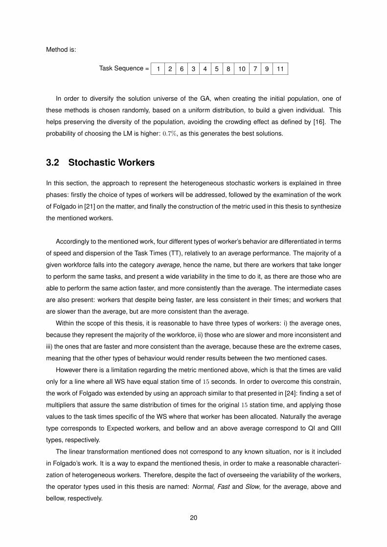
In order to diversify the solution universe of the GA, when creating the initial population, one of

these methods is chosen randomly, based on a uniform distribution, to build a given individual. This

helps preserving the diversity of the population, avoiding the crowding effect as defined by [16]. The

probability of choosing the LM is higher: 0.7%, as this generates the best solutions.

3.2 Stochastic Workers

In this section, the approach to represent the heterogeneous stochastic workers is explained in three

phases: firstly the choice of types of workers will be addressed, followed by the examination of the work

of Folgado in [21] on the matter, and finally the construction of the metric used in this thesis to synthesize

the mentioned workers.

Accordingly to the mentioned work, four different types of worker’s behavior are differentiated in terms

of speed and dispersion of the Task Times (TT), relatively to an average performance. The majority of a

given workforce falls into the category average, hence the name, but there are workers that take longer

to perform the same tasks, and present a wide variability in the time to do it, as there are those who are

able to perform the same action faster, and more consistently than the average. The intermediate cases

are also present: workers that despite being faster, are less consistent in their times; and workers that

are slower than the average, but are more consistent than the average.

Within the scope of this thesis, it is reasonable to have three types of workers: i) the average ones,

because they represent the majority of the workforce, ii) those who are slower and more inconsistent and

iii) the ones that are faster and more consistent than the average, because these are the extreme cases,

meaning that the other types of behaviour would render results between the two mentioned cases.

However there is a limitation regarding the metric mentioned above, which is that the times are valid

only for a line where all WS have equal station time of 15 seconds. In order to overcome this constrain,

the work of Folgado was extended by using an approach similar to that presented in [24]: finding a set of

multipliers that assure the same distribution of times for the original 15 station time, and applying those

values to the task times specific of the WS where that worker has been allocated. Naturally the average

type corresponds to Expected workers, and bellow and an above average correspond to QI and QIII

types, respectively.

The linear transformation mentioned does not correspond to any known situation, nor is it included

in Folgado’s work. It is a way to expand the mentioned thesis, in order to make a reasonable characteri-

zation of heterogeneous workers. Therefore, despite the fact of overseeing the variability of the workers,

the operator types used in this thesis are named: Normal, Fast and Slow, for the average, above and

bellow, respectively.

20

As in the work previously mentioned, the triangular distribution of probabilities is used to describe

the behavior of a human operator. Without too much detail, the choice of this distribution is owed to

the following facts: Naturally, it is more likely for an operator to take a mean time to complete a task,

however, he cannot take an infinite amount of time to complete it, nor can he accomplish the said

task any faster than physically possible, which exclude the normal distribution, thus explaining why the

triangular distribution is the best choice.

The mentioned distribution is described by expression 3.1, where a is the minimum, b the maximum,

c the mode and x the observed time. In this work, the values of a, b and c will be addressed as min, max

and mode, respectively. To compute the time of a given station, the random signal generation block from

simEvents environment was used, as mentioned in 3.3, which has an embedded triangular distribution.

D(x) =

(x− a)2

(b− a)(c− a), if a ≤ x ≤ c.

1− (b− x)2

(b− a)(b− c), if c < x ≤ b.

(3.1)

The triangular distributions proposed by [21] to characterize the Expected, QI and QIII workers can be

consulted in Table 2.1 of section 2.4.1. These served as the base from where to extract the multipliers:

by finding the ratio between each value of minimum, mode and maximum and the average expected

time of 15 seconds. The results obtained can be seen in Table 3.1, where each set is composed of three

values that represent the minimum, mode and maximum of the triangular distribution.

Distribution Min Mode Max

Normal 0.6813 1 1.3187

Fast 0.7181 0.8867 1.2827

Slow 0.6527 1.1593 1.3473

Table 3.1: The multipliers applied to each type of operator.

Regarding the amount of workers of each type present in the workforce, one possible approach is to

have a pool of workers, which have a given price for each type, the fastest being the most expensive,

followed by the normal, and these by the slow workers. If a good configuration of the problem is made:

ratio between prices of workers and amount of workers available, the problem becomes very interesting,

since it weighs the price of investing more in resources, with the increase of productivity.

However, as mentioned, that information is very hard to obtain, implicating a large number of mea-

surements and access to a representative line. Also, the analysis becomes too specific for the problem

at hand, because different lines will very likely have different prices. So, instead, the workforce is defined

with a fixed number of workers, meaning that the problem is to distribute them throughout the line.

3.3 Discrete Event Simulator

The Discrete Event Simulator is used to compute the fitness of each individual, this constitutes a great

advantage, since it allows for a solution based on actual simulation results, instead of one obtained with

21

analytical methods, [56]. This is especially important when dealing with buffers and stochastic workers,

whose randomness makes the alternative process very difficult.

Since the DES is used to evaluate each individual, it has to run individually for each element of the

population, for every generation. If a population of 30 individuals is considered, in 100 generations the

DES would have computed 3000 simulations of the line. This can easily lead to a prohibitive amount

of time to optimize the line. For this reason, one of the main concerns is to develop a model capable

of performing the simulation in a very short interval of time. It is noteworthy that not only the actual

simulation time is important, but also the time spent on communications, both to transfer the results from

the DES to the main GA body, and the other way around.

Therefore, a very streamlined model was developed. Naturally more complex lines can be used

however, at the price of longer optimization times. The lines that are analyzed in this thesis can be

modelled with the following blocks:

• An entity source, that assures that the first WS always has a part to process;

• N Single Servers fed by a random signal generator, to simulate the WS;

• Q = N − 1 FIFO Queues to simulate the Buffers after each WS;

• An entity sink that is never blocked, as a result the buffer of the last WS become redundant, thus

the need for only N − 1 buffers

One feature that largely facilitates the implementation of new lines, is that the AL just has to be

configured once, i.e., the various elements of the line, e.g. servers, buffers, etc, have to be placed on

the respective place, and given an unique name only once, without further need to reconfigure the line

for the rest of the optimization.

The assembly line simulation models are created using the following blocks:

Entity Generator: Responsible for creating the jobs, or parts, that will be processed in the AL. The

entities are generated constantly during the simulation, with a rate higher than the Process Rate of the

line, to assure that the first WS always has a part to process. There is only of Entity Generator at the

beginning of the line.

Random Signal Generator: This block outputs randomly generated numbers based on a triangular

distribution of probabilities that represent the time the adjacent WS took to process a given part at a given

run. The parameters of the distribution (minimum, mode and maximum) are defined by the optimizer.

The Seed used to generate the numbers is randomly generated and stored for reproducibility.

Single Server: The actual workstation is simulated using a Single Server block, fed by the Random

Signal Generator. This way we introduce the stochastic behaviour of the workers in the simulation. The

server holds only the part being processed. It is blocked if the subsequent buffer is full, and starved if no

parts are available in the antecedent buffer.

22

FIFO Queue: The buffers are represented by FIFO Queues, whose capacity is defined by the

optimizer.

Entity Sink: Finally the entity Sink destroys the parts when they reach the end of the AL. It has

infinite capacity, meaning that no buffer is required after the last WS.

In this work the process of building and configuring the line is automatic. A dedicated function

receives as input the desired number of WS, N , it admits that the number of buffers is N−1, and creates

a simple line. An example of a line with 2 WS is showed in figure 3.4, where the various elements of

the line are signalled. This approach is indicated when repetitive lines with more than 3 WS have to be

simulated, since doing it manually is too time consuming and errors are likely to occur.

Figure 3.4: Example of a 2 WS SAL, generated by the ModelBuilder rapid

There are two possible modes to run the DES: normal and rapid. The motivation to create these two

possibilities came from the Simulink logic of normal and accelerator modes, [55]. This allows for faster

simulations when there is no need to interact with the model.

The communication between the Simulink and the Matlab workspace takes a lot of computations; the

solution was to eliminate as much of it as possible. This means that the model is treated as a black box,

i.e., there is no information about the processes that happens inside the model, only about the output.

This approach is possible in this case because the only information required from the simulation is the

WIP and the Cycle Time.

The WIP can be obtained either by observing the number of entities present in each buffer at the

time the simulation ends, and summing that amount, or by simply subtracting the number of destroyed

entities to the number of created entities. The first method allows for a very detailed analysis of the

system, very useful when trying to find bottle necks or other in-line events, however it implies the usage

of communication blocks in each buffer of the line, as well as a great amount of data transfer between

the Simulink environment and the Matlab environment, which slows the computations considerably.

The second requires the usage of only two communication blocks per line, which is acceptable, at

the price of treating the system as a black box. In this work the black box analysis is enough, so all the

communication blocks attached to the buffers were removed.

23

The Cycle Time, like the WIP, can be calculated on a WS event base, or as whole, looking at the

number of parts destroyed and the number of time units the simulation lasted. Of course, as for the

previous Key Performance Indicator (KPI), the first analysis allows for a detailed analysis of the behaviour

of each WS, whilst the second provides information of the line as a whole. More specifically, to calculate

the Cycle Time one can use measured samples of departure events of the last WS, this method is

referred in this work has Last Workstation Cycle Time (LWSCT). Or one can divide the number of parts

created by the number of time units the simulation lasted, thus obtaining the number of parts per unit

of time, which corresponds to the cycle time, this method is referred in this work has Basic Cycle Time

(BCT). The two methods are compared further ahead in section 4.2.

3.4 Genetic Algorithm

In this section the Genetic Algorithm approach will be addressed, for that purpose first the the parallel

processing logic used in work will be explained, the individuals that constitute the population are ex-

plained, then an explanation of the referred procedures is made, as well as of the stopping criteria.

To start an overview of the GA used is presented. The layout is similar to other applications in the

literature, e.g. [28] and [56], with an extra feature: the parallel processing. The flowchart in Figure 3.5

illustrates where the load is spread by the processors, between the New Generation and the Evaluate

Fitness blocks. There the algorithm runs the DES to obtain the throughput of the line, which consumes

the majority of the optimization time. As the simulations are independent of each other, it is possible to

compute them in parallel. There can be as many parallelizations as there as operations, i.e. individuals

to simulate. In this thesis, due to the hardware available, only 4 processors were used.

Figure 3.5: Flowchart of GA

3.4.1 The Initial Population

For the GA to be able to communicate efficiently with the Matlab Workspace, the solutions have to be

conveniently encoded. The entire number of enconded solutions its call the population. The population

of a GA consists of a set of individuals, which on their turn are constituted by chromosomes. The

24

encoding method used here is similar to the one used in [56], but instead of three chromosomes, we

now have four, which are:

• Task Sequence

• WS Sequence

• Worker Type Sequence

• Buffer Capacity Sequence

Task Sequence The first chromosome is the Task Sequence. It was already approached in section

3.1. The output of the task sequence generator is a vector of integers, each representing a specific task,

and that is the vector used as the chromosome. It is important to mention again that the length of the

chromosome is N . Next is showed an example of a Task Sequence chromosome for the line mentioned

in 3.1, the Jackson assembly line. This example is actually of the optimal task sequence for an eight WS

assembly line:

Task = 1 5 4 2 3 6 7 8 10 9 11

WS Sequence The second chromosome is the WS Sequence, as in [56], it is a N × 1 integer

vector, that holds the index of the workstation responsible for each task. To do so, the index in the jth

position of WS Sequence, indicates the WS to which the task in the jth position of Task Sequence is

attributed. This means that the maximum value of this vector is the number of workstations of the line.

To generate this chromosome, the algorithm is has follows:

1. Create a N × 1 random vector, with natural numbers between 1 and M , the number of WS;

2. Test if the vector has at least one of every natural numbers form the interval [1, NumWS], advance

if it does, if not, a new random vector is generated and tested;

3. Sort the vector in ascending order of WS index;

4. END

This method is somewhat different from the one used in [56]. Here the author used a system based

on randomly occurring increments of one unit, as explained next:

1. Start the first slot of the vector with WS(i) = 1, where i = 1;

2. Randomly choose to add 1 or to add 0, i.e. keep the value;

3. If the choice is to add 1, the value of slot WS(i+ 1) is WS(i+ 1) = WS(i) + 1;

4. If the choice is to add 0, the value of slot WS(i+ 1) is WS(i+ 1) = WS(i);

25

5. If all slots have been filled: END. Otherwise, go to step 2.

This is due to the problem addressed here being the ALBP type 2, meaning that there is a fixed

number of WS. This translated into a high number of high indexed WS, since the values that become

higher than the limit during the execution of steps 3 and 4, have to be transformed into values lower than

m. This would imply a solution to distribute those values throughout the several slots, while using a ran-

domly generated vector, assures a balanced distribution of values right from the start, thus constituting

a more efficient solution.

As for the previous chromosome, an example of how an actual WS chromosome might be for the

Jackson line is given. This is optimal distribution of tasks for an eight WS assembly line, provided that

the task sequence is the one presented above:

WS = 1 1 2 3 3 4 4 5 6 7 8

Worker Type Sequence The Worker Type Sequence is where the information about the type of

worker of a given WS is stored. This chromosome was developed in this thesis due to the need to

characterize each worker, thus extending the previously mentioned works.

The types of Workers are defined in the problem setting and were already mentioned in 3.2. The

vector is a M × 1 array of natural numbers, each referring to a type of worker. The correspondence

between the indexes and the types of workers is part of the problem settings. Although, the Normal type

is always defined as being type 1. A feasible Worker Type chromosome if three types of workers are

defined, the first having five operators of the sort, the second just one, and the last two, is exemplified

next:

WType = 1 1 1 2 1 3 2 1

The method used in this work to convert the worker’s performance distribution into actual WS service

times consists of assuming linearity regarding the time each worker takes to perform each task, this

simplification is explained in detail in section 3.2. However, to deal with other problems a more developed

analysis should be made, defining the worker’s performance in a task by task basis.

A possible approach to this problem is to define a 3D matrix, with four layers: k = 1, 2, 3, 4, repre-

senting the four slots columns of the worker matrix presented in 3.2, the minimum, the mode and the

maximum of the triangular distribution in the first three layers, and a natural number representing the

number of operators of a specific type present in the workforce, in the fourth. In each layer the jth col-

umn would hold the times the worker j took to perform each task. And of course, the time task i took

to be performed by each worker would be represented in the ith line. To illustrate, a small example can

be made: to define the triangular distribution of the fourth worker, when performing task number 3, and

26

also the number of workers of that type, the indexes would be:∣∣∣∣∣∣∣∣∣∣∣∣

min = WType(3, 4, 1)

mode = WType(3, 4, 2)

max = WType(3, 4, 3)

number = WType(3, 4, 4)

∣∣∣∣∣∣∣∣∣∣∣∣The rest of the implementation would be quite similar to the one used in this work, the only difference

is that the random times of the tasks assigned to each worker would have to be generated before calcu-

lating the total station time. So that this value inherits the stochasticity of all the elementary operations,

in a task by task basis. It is important to mention that a lot of information is required to perform this

analysis, and that it would be much more complicated to use in this case, so the linear representation is

the best choice.

Buffer Sequence The Buffer Sequence is similar to the one used by [56], apart from an extra

option, that is the possibility of defining the minimal and maximal capacity of the buffers. This feature is

very useful when studying the effect of buffers in a production line. The increase in buffer size usually

translates in an improved Cycle Time, until the optimal is reached. The buffer space has to be defined

by a natural number. The Buffer Sequence chromosome is a M × 1 array of natural numbers, each

referring to the storage capacity of a buffer. A possible solution is:

Buffer = 5 7 1 3 2 8 5 3 1 4 3

3.4.2 Fitness Function

The fitness function consists of the weighted sum of a set of KPIs. The KPIs taken in to account are

explained next.

Cycle Time: The Cycle Time is one of the outputs of the Simulation, and it has already been ad-

dressed in 3.3. The tests were all made in normal mode, meaning that the cycle time used is the Basic

Cycle Time.

Line Efficiency: Percentage of utilization of the line, expressed as the ratio between the total

station time and the cycle time multiplied by the number of workstations:

LE =

∑Ki=1 STi

c×K× 100% (3.2)

where:

STi - Processing Time of WS i;

27

K - Total number of WS;

c - Cycle Time.

Smoothness index: Relative smoothness for a given assembly line. A perfect balance is indicated

by smoothness index 0, and corresponds to a scenario where all the stations have the same time:

SI =

√√√√ K∑i

(STmax − STi)2 (3.3)

where:

STmax - Maximum WS time. In most cases it is the cycle time.

Work In Process: The Work in Process (WIP) has already been addressed in 3.3. The value of

the WIP is given by the difference between the number of entities created and the number of entities

destroyed.

Sum of Buffer Units: Due to the high number of times each individual of the GA has to be eval-

uated, and to the complexity of those individuals, the metric Sum of Buffer Units (SBU) was created in

this work. It provides a fast and representative analysis of the individual, by summing the capacity of

each buffer present in the line. In fact, some solutions might have similar SBU values with different buffer

configurations, in that scenario other KPIs would have to be used to differentiate the solutions.

The fitness function consists of the normalized weighted sum of the KPIs presented. The normaliza-

tion is required because they all have different scales, which would interfere with the weights given. The

KPIs were normalized as showed in equation 3.4:

I(x) =MaxV alue− x

MaxV alue−MinV alue(3.4)

To obtain the maximum and minimum values referred in the expression, the evaluation of the fitness

was made in three steps:

1. Simulate all the individuals using parallel processing, and store the values of the pre-processed

KPIs, in a structure;

2. Look for the maximum and minimum values of each KPI for that generation;

3. Normalize each element as in eq. 3.4.

28

(a) Offspring O1 (b) Offspring O2

Figure 3.6: Example of Crossover process for the Task Sequence Chromosome.

3.4.3 The Crossover Operator

The cross over operator is applied to the selected parents, so that the chromosomes of one parent mate

with the corresponding ones of one other parent. The parents are selected based on their performance

using the Stochastic Uniform Function, which selects the parents randomly with a probability proportional

to their fitness. The crossover fraction, which defines the fraction of individuals in the next generation,

apart from the ones chosen through Elitism, that are created by crossover, is set to 80%. Both the

selection function, and the crossover fraction were tested throughout the development of the algorithm

and obtained the best results. A thorough explanation of both can be found in [54].

Task Sequence The crossing of Task Sequence chromosomes follows a variation of the single

point crossover method as presented in [32]. The method is similar to the one presented by [56]. The

process crosses two parents P1 and P2, to generate two offspring O1 and O2. The main constrain for

the generation of a new task sequence is its feasibility. To assure this, one could either try numerous

combinations to cross the two solutions over in a feasible way, or, on the other hand, one could assure

that the new generation inherits that characteristic from the parents. In order to do so, a random single

cut point is defined, c. In this work, the cut point is bound to the central part of the chromosome, in a

range defined by L4 < c < 3

4L, where L is the length of the chromosome. To guaranty more diversified

solutions. In P1 genes to the left of c are copied directly to the same position in O1, and the same

happens to P2 and O2. Then, and here is where the process diverges from a classical single point

cross over, the genes to the right of the cut point are filled with any element of P2 that has not already

been copied from P1. The mentioned elements are copied to O1 maintaining the order that they had

in P2. The fact of the first half being copied directly from a feasible solution, and the second being

copied maintaining the order it had in a feasible sequence, assures that the offspring is also feasible.

The same method applies to generate O2. To illustrate this process, an example is showed in Figure

3.6, the parents are the two task sequence chromosomes presented in Section 3.1, and they generate

two children:

29


Figure 3.7: Example of Crossover process for the WS Sequence Chromosome.

WS Sequence As before, the method to crossover the WS chromosome utilizes a variation of the

single point crossover method. Here the main constrains are that all the WS have to be present, i.e. all

natural numbers of the interval [1,M ] have to be present, and that they have to be sorted in ascending

order. As for the task sequence crossover operator, two parents, P1 and P2, generate two children, O1

and O2. And the same cut point is used to divide the array in two parts. To generate O1 the genes

to the left of the cut point are copied directly from P1, and the ones to right of c are copied from P2.

The same process is used to generate O2. After that, and here is where the method diverges from the

classical single point crossover, the chromosome is tested for any unfeasible situations, i.e. unsorted

genes and/or missing elements. In case any of this cases is present, the chromosome is corrected

accordingly to a series of criteria. It is important to mention that the only genes that can give origin to an

error are the ones immediately to the right and to the left of c, all the others inherit the feasibility of the

parents.

The example in Figure 3.7, illustrates how the crossover process of the WS chromosome works.

Here the parents were chosen in order to generate one of the mentioned errors. The case is that of

having a missing element in one of the children, namely the WS3 in O2. As the algorithm found three

genes corresponding to WS2, and only one corresponding to WS4, it substituted one of the first mention

genes with the missing WS3. The corrected gene is signaled by the shaded cell.

Worker Type Sequence As was mentioned in 3.4.1, the workforce is fixed, meaning that there is

a determinate number of workers of each type, although, if a method such as a single or double point

crossover was to be applied here, the offspring would likely present unfeasible solutions, e.g. if both

the cuts that are being combined contain workers of only one type, the offspring would not present any

heterogeneous workers. To overcome this problem a different type of operator was developed.

As for the Task and WS operators, this operator generates two children, O1 and O2, from two par-

ents, P1 and P2. Having in mind that the goal of the crossover operator is to generate new solutions

but keeping the genetic print from the parents, and that the main bulk of the workforce is defined in type

1 workers, which correspond to the Normal type. This method starts by finding all the genes corre-

30


Figure 3.8: Example of Crossover process for the Worker Type Sequence Chromosome.

sponding to operators of that type in P1 and P2, and copies them into the same positions of O1 and O2,

respectively. Then, to fill up the rest of the genes, the algorithm copies the remaining genes from P2 into

the vacant positions of O1. The same happens to O2 and P1. The example in Figure 3.8, shows how

the algorithm generates new solutions. The parents are variations of the example introduced in 3.4.1,

where the workforce is defined by three types of workers: the first having five operators of the sort, the

second just one, and the last two, summing up to a total of eight workers. The shaded cells, blue and

green, denote how the position of type 1 workers was inherit by O1 and O2, respectively.

Buffer Sequence The Buffer Sequence Chromosome was generated using a simple single point

crossover operator. In this work the buffers are considered to be all equal along the line, and without

any special need. Therefore there are no main constrains to generate this instance.

3.4.4 Mutation Operator

The mutation operator creates new solutions from random based mutation in order to expand the uni-

verse of solutions. As for the crossover, the mutation operator changes the chromosomes one by one,

therefore they are explained individually.

Task Sequence The method used to mutate the task sequence chromosome is similar to the one

used by [28], and later by [56]. With an additional feature that will be explained farther ahead.

The algorithm first chooses a random task, and finds all the direct successors and predecessors of

that task. Accordingly to what was said in 3.1, for a task sequence to be feasible, all the tasks must follow

all of their direct predecessors and precede all of their direct successors. This means that the chosen

task can occupy any position, as long as it stays within the substring defined by its last predecessor and

its first successor. Having defined that subset the operator changes the position of the selected task

to any of the possible slots, whilst maintaining the order of the rest of the sequence, thus assuring a

feasible solution.

31

The example in Figure 3.9 illustrates the scenario where the original task sequence (parent) is the

optimal one, presented in 3.4.1, and the selected task is task 6. The subset defined by the direct

predecessor, task 2, and the direct successor is signalled. The algorithm chooses a random position in

this subset, in this case it is the left most position, and rearranges the sequence in order to accommodate

the mutation task in the new position, but still maintaining the order of all the other tasks.

Figure 3.9: Example of successful Mutation process for the Task Sequence Chromosome.

The difference introduced in this operator is that when the slot of possible solutions is confined to the

task itself, i.e. there is no freedom to mutate, the algorithm chooses another task to be mutated. It might

be possible that no mutation can be performed, in order to avoid being trapped in a loop the algorithm

only tests a limited number of tasks, in this work we use the limit of 5 loops.

In Figure 3.10, we show a case where this situation takes place. The Mutant is equal to the parent,

so the mutation would be considered unsuccessful and another loop would be performed.

Figure 3.10: Example of unsuccessful Mutation process for the Task Sequence Chromosome.

WS Sequence The WS mutation operator developed for this work is a variation of the classical

methods as presented in [42]. The goal is to orient the search in the direction of the solutions that are

known to be better, e.g. if in a line one WS has a large workload, whilst another has a larger idle time,

it is safe to assume that, transferring tasks from the first to the latter is a good solution. In this work

no special considerations were taken regarding the requirements to perform any of the tasks, thus it is

possible for any workstation to perform any task.

The way the WS chromosome is defined allows for an easy interchange of workload, because the

assignment of the workload is made separately from the task sequence. This means that transferring a

task from one WS to another, does not imply that a specific task will pass form station to the other. Only

that if WSi as n tasks assigned, and WSj has m, if a task is passed from i to j, the workload of the

first will become n − 1 and of the latter m + 1. It is important to mention that the randomness that was

32

to introduced by the mutation operator in a classical scenario, is already taken into consideration in the

crossover operator.

The process operates as follows: the most and least loaded WS are selected, i.e. the one with

highest processing time and the one with the lowest, respectively. Then the number of tasks assigned

to each of the WS is found. If the most heavily loaded one has more than one task assigned, one task

is passed to the least loaded. If it does not, than the WS with the highest number of tasks assigned is

found, and one task from that set is passed to the least loaded WS. After that the new chromosome is

generated and the process finishes.

The example in Figure 3.11 illustrates the process. Assuming that WS7 is the most heavily loaded

one, and that WS3 is the least, the mutation would occur as such:

Figure 3.11: Example of Mutation process for the WS Sequence Chromosome.

Worker Type Sequence Unlike the WS chromosome here it is impossible to know the best search

direction. Therefore, the worker type mutation consists of swaping the position of a Normal worker, with

that of an heterogeneous one. For that, the algorithm starts by finding the position of two workers, one

of type 2 and one of type 1, and than it swaps their position.

Figure 3.12: Example of Mutation process for the Worker Type Sequence Chromosome.

Buffer Sequence The mutation operation regarding the buffer chromosome, due to the lack of

constrains, is made very simply by swapping the position of two randomly chosen elements.

33

3.4.5 Stopping Criteria

Many Stopping Criteria (SC) can be used to terminate the optimization, some related to the performance

of the algorithm, others to time spent running the optimization. The first group is advantageous, since it

allows the GA to wait for a minimum solution to be found, e.g. by setting a limit for the number of times

a specific solution is elected as the best one. While the second group is best suited for time-restricted

optimizations, e.g. by setting a time limit.

As mentioned, the amount of time spent on each iteration, due to the usage of the DES can be very

large. This means that the stopping criteria needs to take into account that a large number of iterations is

unpractical. It is then clear that the criteria should consider the amount of time spent on the optimization.

However, setting a limit of time is not suited for the case at hand, because, it has been observed that the

time each iteration takes depends highly on the performance of the computer being used, thus making

the number of iterations made, impossible to control.

Therefore, the stopping criteria used in this work is the number of generations. The value is set

to 100 across all tests, for it has been deemed sufficiently large, and yet fast enough, allowing a full

optimization to be performed in less than one hour.

3.4.6 Best Solution

By using a given number of generations as stopping criteria, it is possible that the best solution obtained

in the last generation does not correspond to the minimal solution obtained in the whole optimization.

This behaviour can be controlled by setting an appropriate level of elitism, i.e. a percentage of the best

performing individuals that is kept pure for the next generation. However, if the mentioned value is too

high the algorithm is more likely to get trapped in local minima.

Due to the size of the problem considered in this thesis, the choice was to set a value of elitism of

10% of the population, i.e. if there are 30 individuals, the 3 best ones pass to the next generation (for it

obtained the best results), and search for the best solution across all the generations, after the end of

the optimization. This method is used with success in Chapter 4.

Naturally, if the fitness function is the weighted sum of a set of KPIs, a process of normalization is

required. For that end, the same method explained in section 3.4.2 is used. This way the rankings are

preserved, and the choice is guaranteed to be consistent with the optimization made.

3.4.7 Different Approaches Implementation

As mentioned two approaches are developed in this thesis, one of which obtained better results and

therefore was given more attention, named the Two Stages Approach (TSA). The alternative method is

called the One Stage Approach (OSA).

In the TSA, as the name implies, two stages can be differentiated, in the first a classical GA is used

to solve the ALBP-Type II problem. To this end the Task Sequence and WS Sequence chromosomes

are used. The goal is to find the minimal cycle time for the line, which is equivalent to the largest station

time observed. In the second time, after knowing which tasks are made in each WS, from the first stage,

34

a GA coupled with a DES is used to optimize the allocation of buffers and workers to the various WS.

The goal is to minimize the cycle time and the resources used, namely buffer capacity. At this stage

the cost function used, includes the results from the DES, and considers the Worker Type and Buffer

Sequence chromosomes.

The OSA, uses, as the second stage from the alternative method, the DES and the amount of

resources used to compute the fitness function. The difference is that the four chromosomes are con-

sidered simultaneously.

35

Chapter 4

Results Validation on Benchmarking

Lines

In this chapter the performance of the designed algorithm is analyzed, as well as the the effect of

buffers and of the presented heterogeneous workforce. In order to do so it is divided in four main

sections. The first section presents the resources that are used to make the mentioned tests, namely

the benchmarking assembly lines, retrieved from a widely used data base, [44], which are used in this

work, and the different layouts of those lines that are tested. Next, from the two possible DES running

modes presented in section 3.3: normal and rapid, the most suitable one for the study at hand is chosen

by testing and comparing the both alternatives.

In section 4.3 the proposed TSA is compared with another algorithm developed in this work, called

One Stage Approach (OSA). Both methods use the genetic algorithm to minimize a cost function, whose

value is retrieved from the results of the simulation. The main difference between them is that the OSA

approaches the problem as a whole, optimizing the task sequence, tasks and workers allocation to

workstations and capacity of each buffer, hence the name. While the TSA divides it in two, by optimizing

the task sequence and tasks allocation to WS, without resourcing to the DES, and using that solution to

perform the optimization of the worker allocation and buffer capacity much like the alternative method.

The goal of this test is firstly to prove that it is possible to use a OSA, and secondly that, due to the size

and complexity of the problem, TSA the best method.

Afterwards, a set of experiments is made, to evaluate the performance of the TSA algorithm. These

consist of the optimization of the three lines proposed, under different scenarios, called Layouts. Each

Layout represents a different workforce, thus allowing to understand how the system allocates different

workers, and how their presence affects the buffer configuration. The fitness function, as well as the

settings, used are explained in each experiment.

37

4.1 Benchmarking Lines

To test the algorithm, the benchmarking lines retrieved from [44], which is still the standard data set

used by researchers, [35] are used. It is important for the system to perform with lines of different sizes,

and also with different task times, to have a wider range of tests. To that end, three lines were chosen:

Jackson, Mitchell and Gunther. It is noteworthy that the solution for the balancing of the lines has two

parameters, the task sequence and the number of workstations. The instances used in this work are

chosen form a set of possible combinations of these two parameters.

This section is dived in two parts, in the first, the lines are presented and thoroughly explained, and

in the second the tests that feature in this chapter are addressed.

4.1.1 Assembly Lines

Each case is characterized regarding three aspects:i) Number of WS, ii) the Station Time of each WS

and iii) the Task Sequence. The line schemes contain the number of the workstation, which allows a

fast indexation, in the first row, the total cycle time in the second, which is the sum of the time of each

task assigned to a given WS, and the tasks attributed to that workstation in the last one. It is important

to mention that the last row contains the optimal task sequence. The precedence graphs corresponding

to each line can be found in Appendix A.

Jackson This assembly line has 11 tasks, with times ranging from 7 to 1 second. In the data base

the line is optimized for several numbers of stations, here the number of stations used is m = 8. For this

length the optimal configuration without buffers or stochastic task times is:

Workstation 1 2 3 4 5 6 7 8

Station Time 7 7 7 6 6 5 5 4

Tasks 1,5 4 2,3 6,7 8 10 9 11

Table 4.1: Optimal configuration without buffers or stochastic task times for Jackson line.

Mitchell This assembly line has more tasks than the previous: 21 tasks, and they are also more

disperse, with times ranging from 13 to 1 second. Also fot this case, the optimization for several different

numbers of WS can be found in the data set, in this thesis the number used is m = 8, for which the

optimal configuration without buffers or stochastic task times is:


Station Time 13 14 15 15 14 8 13 13

Tasks 1,3 4,5 2,6,7 8,9,11 10,12,15,21 13,16 17 14,18,19,20

Table 4.2: Optimal configuration without buffers or stochastic task times for Mitchell line.

38

Gunther this is largest and with more disperse task times of all the three lines. There are 35 tasks,

with task time values ranging from 1 to 40 seconds. From the set of available configurations, the number

of WS used in this thesis is m = 35. As for the other cases, the optimal configuration without buffers or

stochastic task times is

Workstation 1 2 3 4 5 6 7 8 9 10 11

Station Time 49 48 30 22 49 48 48 49 49 45 48

Tasks 1,5,6 2,3,7,8,10,17 12 9 4,13,14,18 15,16 19,20 11,21,22,25,30 23,24,26,31 27,28 29,32,33,34,35

Table 4.3: Optimal configuration without buffers or stochastic task times for Gunther line.

The following table summarizes the information mentioned above:

Name No of tasks No WS optimal cycle time min tasks time max tasks time

Jackson 11 8 7 1 7Mitchell 21 8 15 1 13Gunther 35 11 49 1 40

Table 4.4: Information of lines to be used.

4.1.2 Presentation of the Layouts

The goal of the developed algorithm is to optimize lines of different sizes, with buffers and stochastic

task times associated with heterogeneous workers. Due to the number of optimization factors, to best

understand the quality of the performance, several scenarios have to be considered. Therefore a set of

layouts were designed, which constitute three different workforces. It is important to mention that the

layouts are part of the problem settings, not an optimization variable. They are explained below:

• Layout 1: All the workers in all three lines are Normal.

• Layout 2: Introduction of one Fast worker, in the case of Jackson and Mitchell lines, and of two

Fast workers in Gunther line.

• Layout 3: Introduction of one Slow worker, in the case of Jackson and Mitchell lines, and of two

Slow workers in Gunther line.

The stochastic workers approach is addressed in 3.2, there, the time distributions corresponding to

each case can be found, together with an explanation of how they were obtained.

4.2 Discrete Event Simulator Testing

As mentioned in section 3.3, the DES can run in two possible modes: normal and rapid. The purpose

of this section is to compare the two modes, and decide which is more suited for this work. From that

analysis the required simulation time for each of the lines presented is computed.

39

The plots in Figure 4.1 show how the Cycle Time calculated by both methods converge to the ex-

pected cycle time asymptotically, the LWSCT from above in red, and the BCT from bellow, in blue. The

data from the graphs was generated by simulating the line with the known optimal distribution, and with

increasingly simulation times. The simulation time is a variable defined in the Simulink model that rep-

resents the time steps computed during the simulation, [55]. The workers used in the analysis are all

equal and deterministic.

(a) JACKSON (b) MITCHELL

(c) GUNTHER

Figure 4.1: BCT (blue) vs LWSCT (red)

The graphs prove that, for these cases, it is possible for the CT to achieve the steady state in both

situations: by resourcing to the internal information of the model (LWSCT), and by treating the system

as a black box analyzing only the inputs and outputs (BCT). Also, it is noticeable that both responses

approach the target CT at the same rate, meaning that the simulation time required for the model to

achieve the steady state is the same, regardless of what method is used.

Therefore, it is safe to say that for these cases, the rapid mode is the best choice, since it produces

the same CT values as the alternative. However, for cases where the internal information of the model

is important the best choice would be to use the normal mode.

The graphs from Figure 4.1 are also used to determine the minimal simulation time required to

accurately simulate each line. This analysis is made by figuring the point where the steady state begins,

i.e. the point where the deviation to the target CT is acceptably small. Naturally, if the simulations ran

40

for as many steps as are showed in the graphs the steady state would be assured, but, as the DES

needs to perform at least a full simulation for each individual every generation, the simulations must be

as expedite as possible. Because of that, it is very important to find a good balance between the amount

of simulation time and the deviation from the steady state behavior.

In the fifth column of Table 4.5 the chosen value of simulation time for each line is showed. The prior

columns show the target CT, the one obtained with the respective simulation time, and also the deviation

between the two, as a ratio. For both Jackson and Mitchell lines, using 1×105 steps proved to be enough

to obtain great precision, however, for Gunther line, due to the higher CT the error incurred is higher,

even with a value of 2.1× 105 steps, but still, the deviation is acceptably small. In the last column of the

table is the Number of Pieces Produced (NPP) during the simulation, for each line.

Line Optimal [sec] Real [sec] Error [%] SimTime NPP

Jackson 7 7.003 0.04 1× 105 14280

Mitchell 15 15.01 0.07 1× 105 7136

Gunther 49 49.1 0.2 2.1× 105 4276

Table 4.5: Information about the simulation time for each line.

4.3 Compare Optimization Methods

In this section the TSA is compared with an alternative approach, named One Stage Approach (OSA),

which was developed because of the strong correlation between the ALBP, the BAP and the allocation

of workers with heterogeneous behaviors. The OSA, however, is proven to be too complex to solve in

a practical time frame for most applications, as well as very sensitive to local minima, due to the large

amount of different configurations that have to be considered.

To compare the two methods the Jackson line was used, with one slow worker and the rest of the

workforce normal. This corresponds to the Layout 3 presented in 4.1, which was chosen because it

represents a situation where buffers have a very important role, due to the effect of the Slow worker. To

allow for a better comparison of the two methods, the maximal initial buffer capacity was set to a very

large value, of 1000 buffer units. This topic is addressed further bellow in section 4.4.2.

The fitness function is the weighted sum of the normalized CT and the normalized overall capac-

ity of the buffers, the SBU, therefore, these two KPIs are taken into consideration to compare the two

methods.The test was repeated 10 times, with different seeds, to have a better understanding of the per-

formance of the algorithm. In the next subsections the results obtained for each method are presented,

first for the One Stage Approach (OSA) and then for the Two Stages Approach (TSA), and finally they

are compared.

41

4.3.1 One Stage Approach

Both the TSA and the OSA consist of coupling a GA and a DES, by using the latter as part of the fitness

function of the metaheuristic. This technique has been used multiple times in literature with success,

e.g. [28] and [56]. In the latter the task sequencing and assignment to WS and the buffer allocation are

solved simultaneously.

Following the same line of thought, the OSA simultaneously tackles the ALBP, BAP and worker

allocation problems. The advantage of this approach is that the task sequence and workstation load can

be adjusted to the presence of buffers and stochastic workers, since even slight changes in the workload

distribution can lead to a more efficient buffer allocation, thus improving the line’s performance, [12].

To evaluate the performance of the algorithm, regarding the minimization of the CT, it is important

to have in mind that the target cycle time is 7 seconds, which might be impossible to achieve due to

the stochasticity of the station times. The test was made under the conditions stated in Table 4.6. It

is important to mention that the weights chosen for the KPIs are merely representative of a plausible

situation where decreasing the CT is more important then having a low number of buffers. However, the

balance between the various indicators is unique for each case, e.g. a factory with limited space might

have to give more importance to the WIP than one without that constrain.

Simulation Time: 100000

Warmup: 400

Population Size: 30

Number of Reps: 3

Number of Generations: 100

Fitness Function: 0.8× CT + 0.2× SBU

Table 4.6: Test conditions.

The final solution obtained with the OSA, for each of the 10 runs can be seen in Table 4.7. The target

CT was achieved only in one instance, which corresponds to the solution with the best score (lowest

fitness value), all other runs propose a value one second slower. The SBU value is clearly not stabilized,

since the level of variation is of about 120%, which means that the highest reported value is about 12

times larger than the smaller.

The best solution, as mentioned, is the one obtained in the second one (in bold), which corre-

sponds to the only one that achieved the target CT of 7 seconds. However, the SBU value of 2294

indicates that the buffers are clearly oversized, the buffer configuration proposed by this solution is:

[837, 60, 85, 283, 731, 266, 32], which, considering the CT and size of the line is clearly exaggerated. The

task assignment and WS times proposed by this solution can be seen in Table 4.8.

42

Run Fitness CT SBU

Run 1 0.178418 8 651

Run 2 0.118742 7 2294

Run 3 0.219917 8 2102

Run 4 0.198038 8 1337

Run 5 0.165634 8 204

Run 6 0.183366 8 824

Run 7 0.178647 8 659

Run 8 0.19392 8 1193

Run 9 0.188371 8 999

Run 10 0.209592 8 1741

Table 4.7: Final Solution obtained with OSA.


Station Time 7 7 7 6 6 5 5 4

Tasks 1,5 2,3 4 6,7 8 10 9 11

Table 4.8: Configuration obtained for Jackson line with OSA.

4.3.2 Two Stages Approach

To analyze the performance of the TSA, the same indicators will be used: the CT and the SBU. However,

considering the nature of the approach, they will be used independently in the first and second stages,

respectively. The line used is the same, as is the test and the genetic algorithm configurations. In table

4.9 that information can be seen.

Stage: 1st 2nd

Simulation Time: NA 100000

Warmup: NA 400

Population Size: 100 30

Number of Reps: NA 3

Number of Generations: 250 100

Fitness Function: CT [0.8× CT + 0.2× SBU ]


First Stage

The first stage consists of determining the optimal task sequence and assignment of tasks to worksta-

tions. This can be achieved by using simple analytical methods, in alternative to the DES. The absence

of buffers and stochastic workers means that no congestion events will take place, therefore the solution

obtained with this method is as good as the simulation based one.

43

The results of the 10 runs are presented here in Table 4.10, for it is more suitable for the case. It

shows that the search was quite successful. In the majority of the cases the optimal solution was found,

and in fact, only one out of the 10 cases presented a sub-optimal solution, that had the minimal error of

1 second. As this is an integer problem, it is impossible to have a error inferior to the unity.

In 90% of the cases the optimal solution was found, 40% of which achieved that value right in the

initial population, and in the remaining runs it was only 1 second off. In this cases, the system took an

average of 3.2 generations to reach the optimal solution. The one case where the final solution was 8

seconds maintained that value since the initial population. Considering all the cases, it can be concluded

that with a 90% probability the algorithm finds the optimal solution in less than 2 generations.

Line % Optimal % Sub-Optimal Av. Gen. to Min.

Jac 0.9 0.1 1.6


As it is possible to see, in what concerns the task sequence and assignment of tasks to workstations,

this method outperforms the OSA by a margin of 80%, since the TSA obtained 90% successful cases,

and the alternative only 10%. Of course, the two solutions cannot be compared until the performance of

the second stage is analyzed.

Second Stage

In the second stage, using the best solution obtained in the first, the algorithm sets the capacity of each

buffer, and allocates the workers to the workstations. However, as mentioned before, the goal of this

section is to compare the two methods, so the only KPIs that will be analyzed are the CT and the SBU,

the analysis of the worker position will only be addressed further ahead.

The analysis of the results, as was made for the OSA, first covers the consistency of the results

across the 10 runs, and, afterwards the best solution found is thoroughly studied. As such, the results

of the 10 runs are presented in Table 4.11.

Also here, the values are quite inconsistent, however with a far smaller amplitude of variation (approx-

imately 35%). It is noticeable that the CT is equal to the target in all runs, meaning that the deviations are

being caused by the SBU value, which values much smaller than those obtained with OSA. The value of

SBU was allowed to achieve very high values in the initial population, therefore it is natural that the op-

timization would require more iterations to bring that value down, as mentioned, this topic is addressed

further ahead. Regarding the best solution, highlighted in bold in Table 4.11, the buffer configuration

for this solution is [3, 7, 1, 1, 1, 1, 1], which is represents a great reduction in relation to the one present

previously.

Both methods, OSA and TSA took about the same time to achieve the results presented. Despite

the fact of the latter having more stages, the first stage, as it uses a simple analytical fitness function, is

very quick, and therefore the time it takes can be disregarded.

However, regarding the CT, with the TSA the target was achieved in 90% of the runs, whereas with

44

Run Fitness CT SBU

Run 1 0.273016 7 30

Run 2 0.225397 7 15

Run 3 0.269841 7 29

Run 4 0.238095 7 19

Run 5 0.250794 7 23

Run 6 0.250794 7 23

Run 7 0.304762 7 40

Run 8 0.253968 7 24

Run 9 0.234921 7 18

Run 10 0.238095 7 19

Table 4.11: Final Solution obtained with TSA.

the OSA only one reached that value. And regarding the buffer allocation, the TSA proposes much

cheaper configurations than the OSA.

Thus, it is safe to assume that the best approach is the TSA. It is important to mention that the

OSA can be useful in certain cases, e.g. when there are worker related constrains, or highly unreliable

machines or operators. When studying those scenarios the OSA offers a great flexibility, since the whole

solution is generated simultaneously taking every factor into account.

4.4 Experiments

In this section a set of Experiments is presented, in order to evaluate the performance of the TSA

on the different scenarios. Each Experiment corresponds to a line being tested for the three possible

Layouts presented in section 4.1. To allow the evaluation of the algorithm with different seeds, 10 runs

were made for each case, this allows for enough sampling and consumes a reasonable amount of time,

approximately 6 hours. Naturally, all the criteria are based on the best individual of each generation, the

others are not considered in this analysis.

The performance evaluation is made by two sets of tests which focus on two different aspects of the

optimization, and are presented next. The first set considers the capacity to explore the whole universe

of solutions (diversification) and the second, the capacity to find the best solutions (intensification). The

nomenclature is similar to that found in [52].

To best explore the diversification capabilities of the algorithm, the respective tests were made with

the maximal initial buffer capacity parameter set to 1000 units, meaning that in the initial population,

the capacity of each buffer is an integer number between 1 and 1000. Obviously, this configuration is

exaggerated, but the goal is to highlight how efficient is the search of a wide universe of solutions.

Three tests were made concerning the diversification: the first regards the minimization of the CT, the

second that of the SBU, and finally the third test shows the best solution found in each run, to evaluate

the consistency of the optimization. The best configuration, naturally, is considered to be the one that

presents the minimal fitness value of all the runs. The tests are presented below:

45

• Amplitude of CT variation: This test consists of computing the ratio between the highest and the

lowest observed cycle times during the 100 generations. This variation is due to the allocation of

buffers and workers, and also to the stochasticity of the times. However, it is important that the

values are low, to support the hypotheses that separating the two stages is possible, since most of

the CT minimization is up to Stg1.

• SBU descent: To evaluate the velocity with which the algorithm searches a solution in a wide

universe, the buffer limit is set to 1000 units, and the evolution of the SBU is plotted for each

generation. It is important for the algorithm to have a good performance here, because, in many

applications the number of buffers required in most of the WS is low, but it is still important to

test other scenarios. A fast descent means that the best solutions start being tested from early

generations.

• Final Solution: The exaggerated limit for the initial buffer capacity, means that the algorithm has

to labor through a lot of iterations until the buffers achieve optimal values. Since the stopping

criteria is the number of generations, it is possible for the optimization to finish before it finds an

acceptable minimum. This test evaluates that possibility.

The second group of tests is dedicated to the intensification of the algorithm, thus it was made with a

much lower maximal initial buffer capacity parameter setting, the value used was 10. This modification

provides the algorithm with a much smaller universe, so that the solutions found are expected to be

better and more consistent among the 10 runs.

The set is composed by two tests, both concerning the final solution, the first assesses the con-

sistency across the 10 runs, and the second analyses the configuration proposed as the best, both in

terms of buffer and worker allocation. It is noteworthy that Layout 1 has a homogeneous workforce, so

the worker allocation analysis is disregarded.

• Consistency of Best Solution: The best solution should be common to all the runs, however, it

is possible for the algorithm to become trapped in local minima, keeping the search from achieving

the same minima in all runs. Therefore, it is important to classify the consistency with which the

solutions are found.

• Best Solution: This is obtained by looking for the minimal fitness value obtained in each run. The

CT, SBU, Buffer allocation and worker positions are analyzed, to understand the reason why the

solution was considered to be the best one.

The first stage (Stg1) and second stage (Stg2) can be analyzed separately, since they are indepen-

dent from each other. This way its possible to better isolate the behavior on each phase. Stg1 will

be presented first, followed by Stg2. This way the latter can be tested using the optimal solution, with

provides more interesting results.

46

4.4.1 First Stage

At this stage, neither the stochasticity of the workers, nor the buffer capacity are considered, so there is

no differentiation between the various layouts, meaning that the only difference between the tests is the

line used. Therefore it makes sense to examine the performance of the system for each one in detail.

The information about the optimal CT was taken from [44].

To assess the quality of the results obtained for the first stage, a set of four parameters will be used.

The tests have all been repeated 10 times with different seeds, each repetition is called a Run. The

metric is based on the values obtained across all repetitions. Each of the mentioned criteria is explained

below:

• The percentage of Runs that achieved the Optimal Solution (ROS).

• The percentage of Runs that achieved a Suboptimal solution with an error inferior to 1 second,

since that is minimum error that can occur, given that this is an integer problem (RSS).

• Average number of Generations until the Optimal Solution (AGOS), regarding the cases where the

optimal solution was actually achieved.

• Average Time spend per Generation (ATG), in seconds.

Jackson

The results of this test were already showed in 4.3.2. There it is possible to see that the algorithm per-

formed well, with 90% of successful runs, that is runs that achieved the optimal. Only once the algorithm

did failed to find the optimal, but it came very close, an error of 1 second, representing approximately

14% of the CT.

In fact, an error of 1 second is the minimal amount of deviation possible, since this is an integer

problem and the smallest unit is 1 second. In Table 4.12 the results are presented using the default

metric:

Code Result

ROS 0.9

RSS 0.1

AGO 2.22

ATG 2.463

Table 4.12: Results of Stg1 with Jackson Line.

Mitchell

Mitchell’s line has more tasks but the same length of line as Jackson’s. The results are showed in Table

4.13. The increase in the number of tasks lead to a slightly worse solution, but still a good one. 70% of

47

the solutions reached the optimal, and, as for the previous case, the ones that did not, had an error of

approximately 7%, which corresponds to 1 second, therefore the minimal error, as as been explained.

Regarding the number of generations until the optimal solution is reached, all the runs in question

reached that value before the 21th generation, only one (Run number 6) took more than that, decreasing

to the optimal value on the 187th generation.

Code Result

ROS 0.7

RSS 0.3

AGO 35.4

ATG 2.470

Table 4.13: Results of Stg1 with Mitchell Line.

Gunther

The large size of Gunther’s line made the problem much harder to solve, thus the solution was worse,

only 30% of the solutions reached the optimal solution. However, none of the runs got a result of more

than 1 second off the optimal, as the optimal CT is 49 seconds, this represents an error of only 2%. Also,

the optimal solution was found with few iterations, an average of about 11 generations.

Thus, the algorithm was able to achieve a good solution all the time, and it did not take many iterations

to reach the optimal in 30% of the tests. These results can be seen in Table 4.14.

Code Result

ROS 0.3

RSS 0.7

AGO 10.7

ATG 2.606

Table 4.14: Results of Stg1 with Gunther Line.

4.4.2 Second Stage

To study the performance of the second stage of optimization, the optimal solution obtained in Stg1 is

used, to make sure that the tests in this subsection are made under optimal circumstances. At this

point the differentiation between the deterministic and stochastic test is important, so each test will be

addressed separately, considering the performance of the algorithm in the three lines, using several

KPIs.

There are many KPIs in the literature, (cf. section 3.4.2), the choice of which is very problem depen-

dent. Since the goal of this work is to evaluate the performance of the algorithm developed, there is not

a detailed analysis of the capabilities of each performance indicator. As the CT is the direct result of

the simulation, naturally, it constitutes an important indicator. This means that the efficiency measures,

48


Warmup: 400

Population Size: 30

Number of Reps: 3



Table 4.15: Test conditions for Experiment 1.

which are not orthogonal to the CT, become redundant. However, it is important to mention that the

other KPIs present in section 3.4.2 can be useful in different cases.

On the other hand, the capacity of buffers of a line is orthogonal to the CT, since the line only has the

capacity to fill the buffer until a certain point, any capacity superior to that value will not affect the CT.

It is equivalent to have an infinity of buffer units available. However it is clearly important to choose the

configuration with the least requirement of buffers, Therefore, the fitness function is the weighted sum

of the CT and the SBU, with a distribution of 80% and 20%, respectively. This configuration represents

a plausible industrial scenario, where achieving a given production rate is more important than having a

low overall buffer capacity.

Other KPIs and weights combinations were experimented throughout the development of the thesis,

which led to the conclusion that this was the most suited combination for this work.

In addition to the two mentioned KPIs, the position of the heterogeneous workers will also be ad-

dressed, because the correct allocation of heterogeneous operators is one of the goals of this algorithm.

It is not, however, part of the fitness function, because the only way to evaluate the quality of the alloca-

tion of the heterogeneous workers is by measuring the effect it has on the CT.

Experiment 1

The first Experiment uses Jackson line, since it is the smallest and, theoretically, the easiest to optimize.

The conditions under which the test were made are presented on Table 4.15. As mentioned, the weights

chosen for the KPIs are merely representative of a plausible situation, and they should be adjusted if a

specific case is to be studied, this also applies to Experiments 2 and 3.

Firstly the amplitude of the CT variation is tested. The results, expressed in Table 4.16, as men-

tioned, show the ratio between the maximum and minimum values observed for the CT across all the

generations of each test. It is possible to see that among all the layouts, the one that produced the

highest amplitude of variation was Layout 3, which is expected, since it contains a Slow worker whose

variability is higher than that of the rest of the workforce.

It is, however, still very small, in the worst case, the minimum value of cycle time found was about

5% smaller than the highest one. Given that part of this variation is due to the stochasticity of the times,

this confirms that the TSA is in fact well founded.

49

Run: 1 2 3 4 5 6 7 8 9 10

Layout 1: 1.014 1.003 1.011 1.018 1.018 1.001 1.018 1.001 1.002 1.001

Layout 2: 1.008 1.001 1.001 1.002 1.014 1.014 1.008 1.001 1.008 1.001

Layout 3: 1.001 1.004 1.052 1.052 1.05 1.053 1.051 1.051 1.053 1.051

Table 4.16: Amplitude of CT Variation, Experiment 1.

The second test of this set concerns the SBU descent, which is made evident by the high initial

values of this variable. As mentioned before, above a critical value, the capacity of the buffer does not

influence the performance of the line, therefore the goal is to find all the solutions that achieve the best

cycle time with minimum buffer units.

In Figure 4.2 the evolution of that value throughout the optimization is showed for each run of Layout

1. It is clear that the values of SBU are descending very fast on early generations, and that they stabilize

as the optimization matures. The final values of these graphs This behavior is expected, since the

amplitude of the values involved in the first generations is much higher, than that of the latter iterations.

There are however some high values, which are attributed to the weight of the CT member of the fitness

function.

Figure 4.2: SBU descent for Layout 1, Experiment 1.

Regarding Layout 2, as can be seen in Figure 4.3, the same type of descent can be found, this time

much clearly. The test presents almost no high SBU values in the last iterations, a part from Run 1,

which depicts a clear descent itself.

50


The SBU descent test for Layout 3 shows the same curve as the two previous tests, but with some

disperse values throughout the space. These take place specially on runs 1,2,4 and 5, which decrease

to lower values on the last generation, as can be seen in Figure 4.4.


It is noticeable that after about the 60th generation, evolution of the SBU for all cases passes form a

curve into a slope like shape. This behavior is due to the consecutive sharing of genes, which leads the

whole population to converge to a common final configuration, and the improvements to be smaller at

each iteration. The neighborhood of the 60th generation, appears to mark the point where the evolution

of the population has stabilize, and most of the improvements are owed to the mutation operator.

Regarding now the Final Solution for the diversification related analysis, in Table 4.17 it is possible to

see the results obtained for all three layouts. Firstly, regarding Layout 1, it is noticeable that the minimal

51

fitness value of 0.24 was achieved by Run 5 and Run 7. This is quite interesting since they both have

higher values of CT, which are balanced by the SBU value of 7. This value means that all buffers have

reached the capacity of 1 unit, which has a toll on the CT.

The Final solution obtained for Layout 2 shows the lack of consistency that was expected, clearly due

to the disperse values of SBU, since the CT is the same for all cases. The consistency of the CT values

is due to the fact, that above a certain value the buffer capacity does not influence the CT. However it is

still remarkable the consistent decrease of SBU values observed in all the runs.

The best solution was obtained in Run 8 (in bold), with a fitness value of 0.215873. The buffer

configuration proposed by this solution is [3, 4, 1, 1, 1, 1, 1], i.e. three units in the buffer that follows WS

1, four in that of WS 2 and 1 unit in the rest. Since the first three WS are the ones with the heaviest

load, they are also the ones with greater variability in times, therefore this configuration makes perfect

sense. And the worker allocation is [1, 2, 1, 1, 1, 1, 1, 1], which means that the Fast worker is actually in

the second WS, rather the third. This explains the high capacity of the buffer adjacent to this WS.

Considering now Layout 3, the values are also quite inconsistent due to the SBU. The best solution

was found in Run 2. The buffer configuration for this solution is [3, 7, 1, 1, 1, 1, 1], which is quite similar

to the one present previously. and the worker configuration is [1, 1, 1, 1, 1, 1, 1, 2], meaning that the Slow

worker was placed on the last WS, which is the one with the lightest load.

Layout 1 Layout 2 Layout 3

Fitness CT SBU Fitness CT SBU Fitness CT SBU

Run 1 0.273016 7 30 0.326984 7 47 0.273016 7 30

Run 2 0.288889 7 35 0.326984 7 47 0.225397 7 15

Run 3 0.247619 7 22 0.257143 7 25 0.269841 7 29

Run 4 0.243175 7.1 8 0.253968 7 24 0.238095 7 19

Run 5 0.24 7.1 7 0.384127 7 65 0.250794 7 23

Run 6 0.339683 7 51 0.273016 7 30 0.250794 7 23

Run 7 0.24 7.1 7 0.238095 7 19 0.304762 7 40

Run 8 0.32381 7 46 0.215873 7 12 0.253968 7 24

Run 9 0.371429 7 61 0.225397 7 15 0.234921 7 18

Run 10 0.27619 7 31 0.292063 7 36 0.238095 7 19

Table 4.17: Final Solution with maximal buffer initial capacity value set to 1000 units, Experiment 1.

Layout 2, includes one Fast worker in the workforce, therefore it is important to know if the algorithm

tends to allocate that operator to right WS, which in this case is WS 3 because it has the highest station

time (7) seconds, alongside with WS 1 and WS 2, but any of the first two WS would translate in an

increase in WIP, due to the third WS becoming slower.

52

In Figure 4.5 (a) the number of times the Fast worker was allocated to a given WS is showed by

means of an histogram. It is clear that the worker is being placed more often in WS 3.

The same applies to Layout 3, but this time a Slow worker is present. This means that this operator

should be placed on the stations with shorter times, to mitigate the effect of the bad performance, both

in terms of speed, and in terms of variability. The behavior of the system regarding this topic can be

observed in Figure 4.5 (b), which shows exactly what has been described: the Slow worker is being

placed, most times in the WS with shorter station times. The last WS is the most visited and it also the

one with the sorter time.

(a) Layout 2 (b) Layout 3

Figure 4.5: Worker Position, Experiment 1

This leads to the conclusion that the system is choosing the best solutions well, in what regards the

placement of the heterogeneous workers, both with Fast and Slow workers. This fact is important be-

cause it assures that the rest of the parameters, CT and SBU, are being tested under the right conditions.

The results obtained on the second set of tests, which evaluates the intensification, are presented in

Table 4.18. As it is possible to see, regarding Layout 1, despite the reduction of the initial buffer capacity,

the results are not consistent across all runs, however, unlike with the previous test made for layout 1

(see Table 4.17), this presents a stable CT of 7 seconds across all runs, which is the target. Also the

SBU is much more stable, oscillating only within 2 units of the value of 16, which represents a great

improvement regarding the consistency of the results. It is interesting to see that none of the solutions

is proposing a line with minimal buffers (SBU = 7), for that has a negative effect on the CT.

Regarding the best solution, which was achieved in Run 5, the respective buffer configuration is:

[5, 3, 2, 1, 1, 1, 1]. It is noteworthy that throughout the other runs, the capacity of the buffers was only

above the unity in the first three buffers, which correspond to the stations with heaviest loads, thus

assuring that those solutions are actually very close to the best one.

The results for the Final Solution for the intensification set of tests, concerning Layout 2, are more

consistent across all the runs. The minimal value was found in three instances: Run 2, Run 3 and Run

9, but also the other runs present very similar results. As expected the CT values are stable, and the

SBU does not deviate more than one unit from a mean value of 10 units.

53

Regarding the Final Solution for this test, despite having the same SBU, the buffer distributions are

different in both cases, runs 2 and 9 present this configuration: [1, 3, 1, 1, 1, 1, 1], whereas Run 3 has

the following: [2, 2, 1, 1, 1, 1, 1]. This means that no difference is detected using this fitness function, in

a real-world case, other criteria would have to be used, e.g. if a buffer capable of holding 3 units costs

more than twice than one that holds 2, the second choice would be cheaper.

The placement of the Fast worker is the same on all solutions: [1, 2, 1, 1, 1, 1, 1, 1]. As mentioned,

this is not considered to be the best location, since WS 3 is slower there is necessarily going to be an

accumulation of WIP between WS 2 and WS 3. It is then concluded that the algorithm is trapped in a

local minimum.

In Layout 3 one Slow worker is present on the workforce, the results for this case are very consistent,

showing the minimal solution across all instances. The buffer allocation for this layout as two possible

configurations: [4, 3, 1, 1, 1, 1, 1] or [3, 4, 1, 1, 1, 1, 1], the same considerations made for Layout 2 apply

here, i.e. another criteria must be used to decide among the two possibilities. The placement of the

Slow worker does not affect the CT, as long as it is confined to last four WS.



Run 1 0.228571 7 16 0.212698 7 11 0.215873 7 12

Run 2 0.234921 7 18 0.206349 7 9 0.215873 7 12

Run 3 0.225397 7 15 0.206349 7 9 0.215873 7 12

Run 4 0.231746 7 17 0.209524 7 10 0.215873 7 12

Run 5 0.222222 7 14 0.212698 7 11 0.215873 7 12

Run 6 0.225397 7 15 0.212698 7 11 0.215873 7 12

Run 7 0.234921 7 18 0.209524 7 10 0.215873 7 12

Run 8 0.225397 7 15 0.209524 7 10 0.215873 7 12

Run 9 0.228571 7 16 0.206349 7 9 0.215873 7 12

Run 10 0.225397 7 15 0.209524 7 10 0.215873 7 12


In Table 4.19 the results obtained are summarized, to provide a global evaluation of the performance

of the algorithm. There it is possible to see the Mean Value (MV) of SBU and Amplitude of Variation

(AV) of the same indicator across all runs of each test individually. The variation is expressed as the

difference between the maximum and minimum observed values for each instance, . The first column

holds the value of SBU for the Initial Population of the Diversification tests (IPD), the second the result of

the optimization made under the same conditions, which is referred as Best Individuals of Diversification

test, and finally the last is the Best Individual of the Intensification tests (BII).

54

Despite the minimal solution not being consistent in all the runs, it shows a remarkable improvement

given the initial population. Regarding first Layout 1, the average value of the SBU on the initial popula-

tion, across all runs, was 2035.3 units, after the optimization that value decreased 98.5%, and the same

can be stated regarding the amplitude of the variation, which decreased 95.3%. A similar behavior can

be seen in Layout 2, the average SBU value decreased 98.8% and the amplitude of the variation 97.0%.

Finally, regarding Layout 3, the initial average SBU and the amplitude of the variation decreased 98.8%

and 97.8%, respectively.

This then leads to the conclusion that in this test, the algorithm proved to be quite capable of search-

ing a wide universe of solutions efficiently, meaning that the diversification of the algorithm is good.

Concerning the other criterion, the intensification, it is possible to conclude that despite the algorithm

not having been able to find a consistent value across all runs, except for layout 3, the solutions are very

similar to each other.


IPD BID BII IPD BID BII IPD BID BII

MV 2035.3 29.8 15.9 2706.6 32 10 2022 24 12

AV 1153 54 4 1743 53 2 1117 25 0

Table 4.19: Evaluation of variation of SBU throughout Experiment 1.

Experiment 2

Experiments 2 and 3 are to a great extent similar to Experiment 1, since the tests are the same and only

the line used differs. Therefore, their presentation is much more expedite disregarding any redundant

explanations. Due to their resemblance with the graphs obtained in the first Experiment, the analysis

of the SBU graphs is briefly summarized here, but the actual figures and respective commentaries are

presented in Appendix B.

The line considered in the second experiment is the Mitchell line. The conditions under which the

tests were made are similar to those of the Experiment 1, and are presented on Table 4.20. Here, the

weights given to the KPIs of the fitness function were chosen to be the same, to be able to compare the

two experiments.

55


Warmup: 400

Population Size: 30

Number of Reps: 3




The first test dedicated to analyzing the diversification of the algorithm, concerns the amplitude of

the variation of the CT. In Table 4.21 it is possible to see that the behavior is similar to that observed

for Jackson line: the larger deviations occur in Layout 3 and are never superior to 5.3%, which supports

the theory that, for the level of stochasticity present in these cases, the line balance obtained in Stg1

corresponds to the optimal.

Run: 1 2 3 4 5 6 7 8 9 10

Layout 1: 1.013 1.013 1.001 1.001 1.013 1.001 1.001 1.001 1.001 1.001

Layout 2: 1.003 1.004 1.003 1.007 1.003 1.007 1.006 1.005 1.009 1.004

Layout 3: 1.051 1.053 1.051 1.002 1.053 1.053 1.051 1.003 1.007 1.051


Regarding the SBU descent, the shape of the curves obtained for all the runs is very similar to that

of Experiment 1, and the same conclusions apply for the three layouts: the descent is very fast in the

early generations, decelerating as it approaches the 60th generation, approximately, decreasing linearly

until the end of the generations. Some values deviate from the main tendency, but all decrease as

the optimization matures. The graphs, alongside with a detailed analysis of each one, can be seen in

Appendix B.1.

The Final Solution obtained with Mitchell line, for the first set of tests, is expressed in Table 4.22.

These samples show that, for Layout 1 the minimization is not yet consistent across all runs, although

Run 1 and Run 2 have the same value, it is not the minimum.

This is actually an interesting situation, for it proves that, in the presence of stochastic workers, if the

line allocates only one unit of buffering between each WS (SBU = 7), the CT increases in 0.2 seconds,

proving the need for more buffering. To give an idea of the effect this increase of CT would have in a real-

world situation, the following calculations can be made: a difference of 0.2 seconds in the production of

each piece, from 15 seconds, to 15.2 seconds, translates into a reduction of about 3 pieces per hour,

which at the end of an 8 hours shift sums up to 24 pieces. This shows how a little increase in the CT

can have a big consequence.

56

The Best Solution is that obtained in Run 5, which allocates a buffer with capacity for 11 units between

WS 3 and WS 4. This configuration makes sense, for these are two WS with heaviest load (station time

of 15 seconds), and consequently with the highest variation of station time.

The Final Solution obtained for Layout 2, despite not being consistent across all runs, all of them

reached the target cycle time, and the highest SUB is 38 in Run 3, considering that the initial SBU value

for that Run in specific was 1858, the descent is considerable, even in the worst case. The position of

the fast worker is the same in all the cases: the Fast worker is placed on WS 4.

The Best Solution of this set (Run 6 in bold), shows a remarkable result, that having only one buffer

per WS (SBU equal to 7 units), which had a negative effect in the CT with all normal workers, does not

have that result when a Fast worker is correctly allocated in the line.

The same test for Layout 3, shows that the system is starting to stabilize, since despite the high initial

values, runs 3 and 10, both achieved the same value of SBU. And also in the other runs the decrease of

the SBU value is remarkable. Run 3 and Run 10 have slightly different buffer configurations, the former’s

is: [1, 2, 6, 1, 1, 1, 1], and that of the latter is: [1, 1, 7, 1, 1, 1, 1]. This result expresses the need for a buffer

between the third and fourth WS that was mentioned above. The worker positioning however was the

same in both cases, WS 6, which is the one with less load, resulting in a diminished effect of the Slow

operator.



Run 1 0.28 15.2 7 0.247619 15 22 0.260317 15 26

Run 2 0.28 15.2 7 0.266667 15 28 0.273016 15 30

Run 3 0.253968 15 24 0.298413 15 38 0.219048 15 13

Run 4 0.266667 15 28 0.250794 15 23 0.333333 15 49

Run 5 0.231746 15 17 0.215873 15 12 0.266667 15 28

Run 6 0.244444 15 21 0.2 15 7 0.234921 15 18

Run 7 0.320635 15 45 0.206349 15 9 0.253968 15 24

Run 8 0.295238 15 37 0.222222 15 14 0.314286 15 43

Run 9 0.269841 15 29 0.215873 15 12 0.247619 15 22

Run 10 0.295238 15 37 0.203175 15 8 0.219048 15 13


As for Experiment 1, the coherence of the allocation of the respective heterogeneous workers has

to be assessed. For that end, Figure 4.6 (a) and (b), show how the algorithm tends to allocate these

operators for Layout 2 and Layout 3, respectively.

The results regarding Layout 2, show that in the great majority of the iterations, the Fast worker was

57

placed on the fourth WS, and since this has the maximal station time (15 seconds) this is the logic place

to allocate the above average worker. In the case of Layout 3, the test shows that the Slow worker is

being placed on all the stations with low times, specially in the sixth. Again, this allocation of workers is

correct, showing that in both instances the solutions are being tested under the right configurations.



Considering now the set of tests designed to assess the quality of the intensification of the algorithm,

Table 4.23. These, as mentioned, were made with a lower maximal initial buffer capacity of 10 units. For

Layout 1, the results show a steady CT of 15 seconds across all runs, and the minimal SBU on three of

them, which, since the CT is constant, are the best solutions found. The rest of the results propose very

similar results, diverting one SBU unit in four cases and two in the three remaining runs.

The best solutions were those found in runs 2, 6 and 8. The buffer configuration is common to all

three: [1, 1, 4, 1, 1, 1, 1], meaning that a buffer with 4 units of capacity is placed between WS 3 and 4.

These correspond to the highest loads, and consequently its where the highest deviations in task times

are. Therefore, it is the optimal positioning of the buffers. It is noteworthy that in all the other runs, the

buffer configuration is similar, varying only the capacity of the third buffer. This proves that the runs are

consistent in terms of buffer placement, showing only a small variation regarding the capacity of some

elements.

Regarding Layout 2, the results show the consistency expected from this test: in all the runs the same

configuration is proposed as the best solution. It is interesting to notice that the same configuration in

the previous test, implicated an increase in the CT (see Table 4.22 regarding Layout 1). This means that

the allocation of a Fast worker to the third WS is enough to balance the line.

The results obtained for Layout 3 are not as consistent, however half the runs found the best solution,

and the other half was also able to achieved the optimal CT, but with two more SBU units. The configu-

ration of the buffers is also very similar between the to solutions, the one proposed by the best solution

is [1, 1, 6, 1, 1, 1, 1], and the other is [1, 1, 8, 1, 1, 1, 1]. The worker allocation is not consistent throughout

the various runs, varying among the WS with lightest loads. Here again, the KPIs used are not capable

of distinguishing among the various solutions, meaning that if a choice has to be made, more criteria are

58

in order, e.g. social factors.



Run 1 0.215873 15 12 0.2 15 7 0.215873 15 12

Run 2 0.209524 15 10 0.2 15 7 0.222222 15 14

Run 3 0.212698 15 11 0.2 15 7 0.215873 15 12

Run 4 0.212698 15 11 0.2 15 7 0.215873 15 12

Run 5 0.212698 15 11 0.2 15 7 0.222222 15 14

Run 6 0.209524 15 10 0.2 15 7 0.215873 15 12

Run 7 0.215873 15 12 0.2 15 7 0.222222 15 14

Run 8 0.209524 15 10 0.2 15 7 0.215873 15 12

Run 9 0.215873 15 12 0.2 15 7 0.222222 15 14

Run 10 0.212698 15 11 0.2 15 7 0.222222 15 14


As for the previous experience, the results are here summarized to give an overview of the perfor-

mance of the algorithm throughout the experiment. From Table 4.24, it is possible to conclude that also

with a larger amount of tasks, 21 tasks, the algorithm is capable of searching a very wide universe of

solutions efficiently. In the first set of tests, as can be seen by comparing the IPD and the BID columns,

the SBU value, decreased significantly both in average value and in amplitude of variation among runs.

For Layout 1, those values are: 98.7% and 97.1%, respectively. The came can be said for Layouts 2 and

3, the former presents a decrease of 99.42% regarding the average SBU value, and of 98.9% regarding

the amplitude of variation, and the latter 98.7% and 96.9%, respectively.

This is a strong indicator of a good diversification, meaning that the algorithm is able to efficiency

search a wide universe of solutions. Regarding the evaluation of the intensification, the results show

that the system was able to concentrate the solutions in a small neighborhood, however, only on Layout

2 full consistency was achieved.



MV 1906.2 25.2 10.8 2983.6 17.3 7 2035.3 26.6 13

AV 1293 38 2 2917 31 0 1153 36 2


59

Experiment 3

This Experiment is made considering Gunther line, under the conditions expressed on Table 4.25. As

mentioned in Experiment 2, the analysis is very similar to the ones already made, therefore, to avoid

redundancies, some of it is made in a more summarized fashion. Namely, the study of the evolution

of the SBU value throughout the optimization, is mentioned here, but the full analysis can be found in

Appendix B.


Warmup: 400

Population Size: 30

Number of Reps: 3




Following the same scheme as before, the diversification of the algorithm is assessed first. Regarding

the amplitude of the CT variation for the 10 runs of this experiment, the results, expressed in Table 4.26,

show that the highest variation occurred in the third layout, and was sufficiently small, about 5%, to

support the stage division.

Run: 1 2 3 4 5 6 7 8 9 10

Layout 1: 1.004 1.003 1.01 1.009 1.003 1.007 1.003 1.01 1.003 1.007

Layout 2: 1.004 1.013 1.004 1.004 1.004 1.006 1.007 1.002 1.003 1.003

Layout 3: 1.051 1.049 1.049 1.049 1.047 1.051 1.047 1.032 1.051 1.032


The shape of the curves obtained for the SBU Descent test, is very similar to that of the previous

two experiments, and so are the conclusions to be taken form analyzing them. The tests show that for

all three Layouts the evolution is very fast in the early generations, the descent decelerates as it ap-

proaches the 60th generation, approximately, and shows a linear behavior since. As for the other cases,

some values deviate from the main tendency, but all decrease eventually. The graphs, alongside with a

detailed analysis of each one, can be seen in Appendix B.2.

Considering now the Final Solution for the first analysis, in Table 4.27 it is possible to see the results

obtained for all three layouts. Regarding Layout 1, it is noticeable that at each Run had a different result,

meaning that no conclusions can be made regarding the optimal configuration. This was the expected

result, since the initial parameters were set to unreal values. The CT of all the runs are considerably

close to target value of 49 seconds, with a maximum deviation of about 1%.

The lowest value obtained took place in the seventh run, and it is interesting to see that it presents

60

the same SBU value as Run 2, but this has a higher CT, which given the fitness function, results on a

worse score. The reason for this classification is the allocation of the buffers, as mentioned, the SBU

accounts only for the overall amount of buffers in the line, to decide on the best configuration is up to the

CT member of the function. The configuration of the best solution, Run 7 is [13, 1, 1, 1, 4, 2, 7, 3, 1, 2], the

capacity of the first buffer is exaggerated, but in all the other cases where the CT was 49.2, this value

was of 3 units. Thus, it is concluded that the difference between the two instances lies in the fact that

the first WS, due to its large load has a great variance, and the station time of WS 2 is not small enough

to deal with that variance, therefore, if no buffers are present, it is likely that blocking events take place.

An interesting fact about the results of Layout 2, is that they show consistently shorter CT values,

across all runs, when compared to those of Layout 1. This effect is attributed to the presence of the

fast workers, allocated to the stations with heaviest loads. The best solution was obtained in Run 9, and

its buffer configuration is [10, 1, 5, 1, 1, 2, 9, 22, 1, 1]. Notice the capacity of the first buffer, and that of the

seventh and eight, which correspond to the high load areas. Regarding the worker allocation, one Fast

worker was placed on the first WS and the other on the fifth, since these are two of the most slow, the

allocation is deemed to be correct.

Considering Layout 3, as can be concluded form the results, the CT values are comparable to those

of Layout 1, however slightly worse, due to the presence of Slow workers. The best solution is that found

in Run 6, which achieved a CT of 49.3 seconds with an SBU of 24 units. These units are distributed as

follows: [9, 1, 1, 1, 2, 1, 2, 5, 1, 1], and the Slow workers were allocated to WS 3 and WS 4, which have the

shortest times attributed.



Run 1 0.431111 49.2 78 0.426667 49.1 94 0.382222 49.3 38

Run 2 0.375556 49.3 35 0.608889 49.2 158 0.546667 49.4 94

Run 3 0.362222 49.3 29 0.493333 49.1 124 0.546667 49.4 94

Run 4 0.673333 49.5 133 0.342222 49.1 56 0.575556 49.6 71

Run 5 0.42 49.2 73 0.435556 49.1 98 0.524444 49.4 84

Run 6 0.411111 49.4 33 0.455556 49.1 107 0.351111 49.3 24

Run 7 0.335556 49.2 35 0.468889 49.1 113 0.506667 49.4 76

Run 8 0.502222 49.5 56 0.677778 49.2 189 0.444444 49.3 66

Run 9 0.404444 49.2 66 0.335556 49.1 53 0.526667 49.4 85

Run 10 0.537778 49.5 72 0.362222 49.1 65 0.455556 49.4 53


The analysis of the worker allocation, for layouts 2 and 3 can be seen in Figure 4.7 (a) and (b),

61

respectively. Has for the previous experiments, it shows a correct tendency, by placing the Fast workers

in the WS with the heaviest loads, and the Slow in those where the station time is shorter. Therefore, it

is concluded that the buffer allocation is being made under the correct circumstances.



The tests presented next regard the quality of the intensification of the algorithm. Regarding Layout

1, Table 4.28 shoes that the majority of the runs achieved the best solution. This result is considered to

be very good, given the size of the line. And it is noteworthy that the rest of the cases presented a very

similar result, with only one unit of SBU above, and the same CT. All the best solutions were achieved

with different buffer configurations, which are presented below:

• Run 1 - [3, 1, 1, 1, 4, 3, 3, 6, 2, 1]

• Run 2 - [4, 1, 1, 1, 2, 3, 7, 4, 1, 1]

• Run 4 - [2, 3, 1, 1, 4, 3, 3, 6, 1, 1]

• Run 5 - [3, 1, 1, 1, 6, 2, 4, 5, 1, 1]

• Run 6 - [2, 2, 1, 1, 5, 2, 5, 5, 1, 1]

• Run 8 - [2, 1, 1, 2, 3, 3, 5, 5, 2, 1]

It is noticeable that WS 1, and WS 5 to WS 8, never have the minimal capacity of one unit, this is

clearly due to fact of these having a heavy load attributed. As mentioned, to distinguish among these

alternatives another criteria has to be defined, e.g. price of buffers accordingly to their size.

Regarding Layout 2, the best solution is common to three instances, runs 2, 3 and 7. Like for the

previous case, the CT are consistently shorter than those of the Layout 1, which supports the hypotheses

presented, that the Fast operators are able to decrease the CT. The same can be verified for the SBU

values: this are smaller than the ones obtained for the first layout.

For this layout, the best solutions have the same placement of the Fast operators: WS 5 and 8, which

both have a station time of 49 seconds. As for Layout 1. there are three different buffer configurations,

presented below:

62

• Run 2 - [2, 1, 1, 1, 1, 1, 2, 2, 1, 1]

• Run 3 - [3, 1, 1, 1, 1, 1, 1, 2, 1, 1]

• Run 7 - [2, 1, 1, 1, 1, 1, 1, 3, 1, 1]

These probably whoud be improved if instead of being in WS 8, the Fast worker was placed in WS

9, for this would allow for a smaller buffer in WS 8. This however could give rise to this worker being

starved, thus harming the CT.

The results obtained for Layout 3 show that the CT is worse that that of Layout 1, which reflects

the effect of the two Slow workers in the line. The SBU values, however are similar. The best solution

was achieved in Run 1 and Run 4, with a CT of 49.4 seconds, and an SBU value of 23 units. All other

instances where the SBU showed a smaller value, have worst CT, resulting in worst overall score.

Run 1 and Run 4, have different buffer configurations [3, 1, 1, 1, 2, 4, 3, 5, 1, 2] and [4, 1, 1, 1, 3, 2, 4, 5, 1, 1],

respectively. Here also, the more heavely loaded WS are followed by large buffers, which explains why

these solutions are the best ones. The worker allocation, on the other hand is common to both cases,

placing the two Slow operators in the third and fourth WS.



Run 1 0.353333 49.3 25 0.288889 49.2 14 0.388889 49.4 23

Run 2 0.353333 49.3 25 0.246667 49.1 13 0.391111 49.4 24

Run 3 0.355556 49.3 26 0.246667 49.1 13 0.424444 49.5 21

Run 4 0.353333 49.3 25 0.293333 49.2 16 0.388889 49.4 23

Run 5 0.353333 49.3 25 0.255556 49.1 17 0.4 49.4 28

Run 6 0.353333 49.3 25 0.291111 49.2 15 0.391111 49.4 24

Run 7 0.355556 49.3 26 0.246667 49.1 13 0.4 49.4 28

Run 8 0.353333 49.3 25 0.26 49.1 19 0.4 49.4 28

Run 9 0.355556 49.3 26 0.291111 49.2 15 0.415556 49.5 17

Run 10 0.355556 49.3 26 0.3 49.2 19 0.397778 49.4 27


In the previous experiments the CT kept constant and equal to the target in the vast majority of the

cases, in this case however, it showed a slight variation throughout the various tests. This behavior

is due to the linearity assumed to describe the stochasticity of the workers (cf. section 3.2), which,

because of the high CT of Gunther line, translates in a high deviation of the station times, thus giving

rise to starvation and blocking events.

The performance of the algorithm regarding this topic, can be evaluated by the convergence of the

63

values obtained in the various runs, which indicate whether the system has found a global minimum,

or local one. The diversification tests, do not give a precise information about the CT, since, in those

test, the buffer capacity is exaggerated in order to amplify the search space, thus leading to a virtual

improvement of the CT. Therefore, the criterion is the performance in the intensification tests. Which,

due to the consistency of the CT across all runs of each respective test, leads to the conclusion that the

system is able to minimize the CT efficiently.

However, since the variation of the CT is vestigial when compared to that of the SBU (see Table

4.26), the latter is more significant for the evaluation of the algorithm’s performance. In Table 4.29, as

for the previous experiments, the overview of the evolution of the SBU is given. There it is possible to

see that the solutions are converging significantly, by comparing the IPD with the BID. In the first layout

the average of the SBU and the amplitude of variation decreased 98.0% and 92.1%. Regarding Layout

2, those values were 97.7% for the average and 94, 45% for the amplitude of variation. Finally Layout 3

had a similar behavior: average SBU value decreased 98.2% and the amplitude of variation 96.0%.



MV 3032.5 61 25.4 4596 105.7 15.4 3991.4 73.2 24.3

AV 1320 104 1 2451 136 6 2240 90 11


In all three experiments, the TSA showed very good results regarding the diversification criterion,

thus proving that it is an appropriate tool to deal with large-sized problems, like Gunther line. The same

cannot be said for the intensification criterion, since the target consistency across the 10 runs was

achieved only in two instances. However, in the intensification tests, the results were all within a small

neighborhood, meaning that the problem could easily be solved with normal heuristics.

Regarding the configuration of the buffers, it is noticeable that, across the three experiments, the

best solutions tend to allocate most of the capacity to the areas which follow WS with high processing

times. This way, the effect of the great variability of these WS does not propagate to the rest of the line.

Finally, considering the positioning of the Fast and Slow workers, the best solutions across all ex-

periments show a similar tendency: The Fast workers are placed in the WS with higher loads, because

these are the bottlenecks that limit the production rate of the AL. Whereas the Slow workers are kept

in the WS with shorter processing time, this assures that despite their performance, the effect of these

workers is minimized.

64

Chapter 5

Conclusions

The goal of this thesis centres in the development and application of a genetic algorithm based method

to solve the Assembly Line Balancing Problem (ALBP) Type II, with intermediate buffers, stochastic

task times and heterogeneous workers. The method consists of two stages which use the mentioned

metaheuristic algorithm to minimize a cost function.

In the first stage a GA developed in Matlab is used to solve the ALBP-Type II, by finding the se-

quencing and allocation of tasks to a given number of WS that minimizes the CT of the line, without

considering any stochasticity regarding the times, nor the presence of buffers. The fitness value is the

CT of the line, which is equivalent to the processing time of the WS with the heaviest load, and it is

computed by summing the times of the tasks assigned to that WS.

In the second stage a DES model is coupled to a GA, to compute the fitness of each individual by

simulating the line. The objective of the optimization is to minimize the CT and the overall capacity of the

buffers of the AL defined in the first stage, by finding the best buffer configuration and worker allocation.

The cost function is consists of the weighted sum of the CT and the overall capacity of the line’s buffers,

Sum Of Buffer Units (SBU).

The SBU provides a good metric to compare a high number of different configurations in a small

interval of time, by focusing on the overall capacity of all the buffers instead of analyzing each buffer

individually. It is, however, unable to distinguish configurations that despite having the same global

buffer capacity, present a different allocation of that capacity.

Using the DES model to compute the CT of each individual of each generation, allows for a very

precise evaluation of the line, which takes into account starving and blocking phenomena. It also as-

sures a great flexibility concerning the size and complexity of the lines, since these features are easily

implemented in the model.

To minimize the capacity of each buffer, the metric used is based on the fact that above a certain

volume, increasing the capacity of a buffer does not produce any effect on the line’s performance. How-

ever, if the capacity of the buffer is too low, blocking and/or starvation phenomena take place, resulting

on an increased CT.

The proposed method has been compared with another that solves the task sequencing and distri-

65

bution, the buffer and the workforce allocation problems simultaneously. The advantages of this method

are stated, but it is proven not to be the best approach for the benchmarking cases used.

Nine scenarios are used to test the proposed algorithm, each constituted by a given assembly line

and workforce layout. The assembly lines are benchmarking cases with: i) different sizes; ii) distinct

cycle times; and iii) three possible workforce layouts, namely: a) with all average workers, b) with one

above average worker and the rest average c) with one below average worker and the rest average.

Due to the lack of quantitative studies considering heterogeneous workers, and the difficulty of ob-

taining enough information to characterize a workforce, in terms of performance -speed and deviation

of task times, the results obtained in Folgado [21] are extended to define a speed factor relative to the

average worker, which is then applied to each case to characterize the behavior of each member of the

workforce.

The performance of the proposed method is analyzed according to two criteria: the capacity to search

the universe of solutions, which is referred as diversification, and the ability to find optimal solutions,

called intensification. The results obtained for both are evaluated using the consistency across ten runs

started with different seeds, and the quality of the best solution found across all the runs. This allows to

assess if the algorithm is evolving in the direction of a minimum, and if that is a local or a global minima.

To evaluate the diversification a wide universe of solutions is created, by allowing the capacity of the

buffers in the initial population to achieve very high values (1000 units), which places these solutions

very far from the optimal. The results show that even with this settings the system is able to consistently

narrow down the search space, presenting reductions of the average overall capacity of the line’s buffers,

across the whole population, between 97.70% and 99.42%, and concerning the variability of the same

result the observed reductions range between 92.12% and 98.94%.

The intensification is evaluated by starting the population with a much lower number of buffer units

(10 units), thus bringing it closer to the optimal value. The results show that, regarding the cycle time, 7

of the 9 tests have perfectly consistent values across all runs, and that the ones that deviated, did it only

by 0.2% of the line’s cycle time. Concerning the buffer capacity, the results were perfectly consistent in

2 of the 9 cases, had a maximum amplitude of variation of 4 units across the 10 runs in 5 other cases,

and in the two tests which obtained different cycle times, that amplitude raised to 6 and 11 units.

This then leads to the conclusion that, the algorithm is highly capable of tackling a wide number of

possible solutions, but, despite being able to provide a good balance of the line and its components,

the best configuration is not always consistent. This behavior is attributed to the lack of precision of the

KPI used to evaluate the buffer configuration, mentioned above. However, given the small neighborhood

of the final results, the problem is likely to be solved by heuristics which guarantee an optimal line

configuration.

5.1 Future Work

Given the promising results achieved in this thesis, regarding the usage of metaheuristics and simulation

to balance complex assembly lines, the first proposed step to improve the model is to further develop

66

the KPIs regarding the evaluation of the buffer configuration, so that they can be distinguished more

precisely.

In second place, it is suggested to approach the Mix Model Assembly Line Balancing Problem, which

considers the processing of more than one model in the assembly line, for it has been referred in a large

number of studies made on the last years, and compare the algorithm developed with the benchmarking

methods. It is proposed to follow an approach similar to one found in Tiacci [56] to implement this feature

in the algorithm presented in this thesis.

When the behavior of a workforce is studied, an important factor to take into account is the expe-

rience of the workers. In Hopp et al. [24] a strategy to deal with accumulating WIP between WS is

presented, based on policies to train certain workers to preform tasks on multiple WS, which are reallo-

cated temporarily to deal with congestions. As future work it is proposed to develop the model in order to

assimilate this knowledge, allowing the line manager to decide where to place such workers, in order to

achieve a number of objectives, as: maximize the influence of the mentioned workers or minimize their

dislocations, among others.

Lastly, it is proposed to apply the algorithm developed to a real-world case of AL reconfiguration,

where, despite the added complexity characteristic of this type of problems, the presence of more deci-

sion variables, e.g. economical factors, allows to further develop the KPIs, and consequently the fitness

function.

67

Bibliography

[1] Kursad Agpak and Hadi Gokcen. A chance-constrained approach to stochastic line balancing

problem. European Journal of Operational Research, 180(3):1098–1115, 2007.

[2] Sener Akpınar and G Mirac Bayhan. A hybrid genetic algorithm for mixed model assembly line

balancing problem with parallel workstations and zoning constraints. Engineering Applications of

Artificial Intelligence, 24(3):449–457, 2011.

[3] Sener Akpınar, G Mirac Bayhan, and Adil Baykasoglu. Hybridizing ant colony optimization via ge-

netic algorithm for mixed-model assembly line balancing problem with sequence dependent setup

times between tasks. Applied Soft Computing, 13(1):574–589, 2013.

[4] Tayfur Altiok and Shaler Stidham Jr. The allocation of interstage buffer capacities in production

lines. AIIE Transactions, 15(4):292–299, 1983.

[5] Maghsoud Amiri and Ali Mohtashami. Buffer allocation in unreliable production lines based on

design of experiments, simulation, and genetic algorithm. The International Journal of Advanced

Manufacturing Technology, 62(1):371–383, 2012.

[6] Jerry Banks. Handbook of simulation: principles, methodology, advances, applications, and prac-

tice. John Wiley & Sons, 1998.

[7] Daria Battini, Alessandro Persona, and Alberto Regattieri. Buffer size design linked to reliability

performance: A simulative study. Computers & Industrial Engineering, 56(4):1633–1641, 2009.

[8] Ilker Baybars. A survey of exact algorithms for the simple assembly line balancing problem. Man-

agement science, 32(8):909–932, 1986.

[9] Christian Becker and Armin Scholl. A survey on problems and methods in generalized assembly

line balancing. European journal of operational research, 168(3):694–715, 2006.

[10] Christian Blum and Cristobal Miralles. On solving the assembly line worker assignment and bal-

ancing problem via beam search. Computers & Operations Research, 38(1):328–339, 2011.

[11] Nils Boysen and Malte Fliedner. A versatile algorithm for assembly line balancing. European

Journal of Operational Research, 184(1):39–56, 2008.

69

[12] Nils Boysen, Malte Fliedner, and Armin Scholl. Assembly line balancing: Which model to use

when? International Journal of Production Economics, 111(2):509–528, 2008.

[13] J Bukchin. A comparative study of performance measures for throughput of a mixed model as-

sembly line in a jit environment. International Journal of Production Research, 36(10):2669–2685,

1998.

[14] John A Buzacott and J George Shanthikumar. Stochastic models of manufacturing systems, vol-

ume 4. Prentice Hall Englewood Cliffs, NJ, 1993.

[15] Wen-Chyuan Chiang. The application of a tabu search metaheuristic to the assembly line balancing

problem. Annals of Operations Research, 77:209–227, 1998.

[16] Kenneth Alan De Jong. Analysis of the behavior of a class of genetic adaptive systems. Technical

report, The University of Michigan, Computer and Communication Sciences Department, 1975.

[17] Leyla Demir, Semra Tunali, and Deniz Tursel Eliiyi. The state of the art on buffer allocation problem:

a comprehensive survey. Journal of Intelligent Manufacturing, 25(3):371–392, 2014.

[18] Kenneth H Doerr and Antonio Arreola-Risa. A worker-based approach for modeling variability in

task completion times. IIE Transactions, 32(7):625–636, 2000.

[19] Marco Dorigo, Vittorio Maniezzo, and Alberto Colorni. Ant system: optimization by a colony of

cooperating agents. Systems, Man, and Cybernetics, Part B: Cybernetics, IEEE Transactions on,

26(1):29–41, 1996.

[20] George Fishman. Discrete-event simulation: modeling, programming, and analysis. Springer Sci-

ence & Business Media, 2013.

[21] R Folgado. Heterogeneity and Variability on Human-Centered Assembly Systems. PhD thesis,

Instituto Superior Tecnico, 2012.

[22] Fred Glover, Manuel Laguna, E Taillard, and D De Werra. Tabu search. Baltzer Basel, 1993.

[23] Nima Hamta, SMT Fatemi Ghomi, F Jolai, and M Akbarpour Shirazi. A hybrid pso algorithm for a

multi-objective assembly line balancing problem with flexible operation times, sequence-dependent

setup times and learning effect. International Journal of Production Economics, 141(1):99–111,

2013.

[24] Wallace J Hopp, Eylem Tekin, and Mark P Van Oyen. Benefits of skill chaining in serial production

lines with cross-trained workers. Management Science, 50(1):83–98, 2004.

[25] S Jack Hu, J Ko, L Weyand, HA ElMaraghy, TK Lien, Y Koren, Hl Bley, G Chryssolouris, N Nasr,

and M Shpitalni. Assembly system design and operations for product variety. CIRP Annals-

Manufacturing Technology, 60(2):715–733, 2011.

[26] James R Jackson. A computing procedure for a line balancing problem. Management Science, 2

(3):261–271, 1956.

70

[27] David C Juran and Lee W Schruben. Using worker personality and demographic information to

improve system performance prediction. Journal of Operations Management, 22(4):355–367, 2004.

[28] Yeo Keun Kim, Yong Ju Kim, and Yeongho Kim. Genetic algorithms for assembly line balancing

with various objectives. Computers & Industrial Engineering, 30(3):397–409, 1996.

[29] Scott Kirkpatrick. Optimization by simulated annealing: Quantitative studies. Journal of statistical

physics, 34(5-6):975–986, 1984.

[30] Sophie D Lapierre, Angel Ruiz, and Patrick Soriano. Balancing assembly lines with tabu search.

European Journal of Operational Research, 168(3):826–837, 2006.

[31] Cristobal Miralles, Jose Pedro Garcia-Sabater, Carlos Andres, and Manuel Cardos. Advantages

of assembly lines in sheltered work centres for disabled. a case study. International Journal of

Production Economics, 110:187–197, 2007.

[32] Melanie Mitchell. An introduction to genetic algorithms. MIT press, 1998.

[33] Ozcan Mutlu, Olcay Polat, and Aliye Ayca Supciller. An iterative genetic algorithm for the assembly

line worker assignment and balancing problem of type-ii. Computers & Operations Research, 40

(1):418–426, 2013.

[34] Armin Scholl Nils Boysen, Malte Fliedner. A classification of assembly line balancing problems.

European Journal of Operational Research, 183:674–693, 2007. doi: 10.1016/j.ejor.2006.10.010.

[35] Alena Otto, Christian Otto, and Armin Scholl. Systematic data generation and test design for so-

lution algorithms on the example of salbpgen for assembly line balancing. European Journal of

Operational Research, 228:33–45, 2013.

[36] Peng Si Ow and Thomas E Morton. Filtered beam search in scheduling†. The International Journal

Of Production Research, 26(1):35–62, 1988.

[37] Ugur Ozcan. Balancing stochastic two-sided assembly lines: A chance-constrained, piecewise-

linear, mixed integer program and a simulated annealing algorithm. European Journal of Opera-

tional Research, 205(1):81–97, 2010.

[38] Chrissoleon T Papadopoulos, Michael EJ O’Kelly, Michael J Vidalis, and Diomidis Spinellis. Analy-

sis and design of discrete part production lines. Springer, 2009.

[39] HT Papadopoulos, Jimmie Browne, and Cathal Heavey. Queueing theory in manufacturing systems

analysis and design. Chapman & Hall, 1993.

[40] Taeho Park. A two-phase heuristic algorithm for determining buffer sizes of production lines. THE

INTERNATIONAL JOURNAL OF PRODUCTION RESEARCH, 31(3):613–631, 1993.

[41] Michael Pinedo. Planning and scheduling in manufacturing and services, volume 24. Springer,

2005.

71

[42] Riccardo Poli, William B Langdon, Nicholas F McPhee, and John R Koza. A field guide to genetic

programming. Lulu. com, 2008.

[43] Melvin E Salveson. The assembly line balancing problem. Journal of Industrial Engineering, 6(3):

18–25, 1955.

[44] Armin Scholl. Data of assembly line balancing problems. 1993.

[45] Armin Scholl and Christian Becker. State-of-the-art exact and heuristic solution procedures for sim-

ple assembly line balancing. European Journal of Operational Research, 168(3):666–693, 2006.

[46] Armin Scholl and Stefan Voß. Simple assembly line balancing—heuristic approaches. Journal of

Heuristics, 2(3):217–244, 1997.

[47] Armin Scholl, Nils Boysen, and Malte Fliedner. The sequence-dependent assembly line balancing

problem. OR Spectrum, 30(3):579–609, 2008.

[48] Armin Scholl, Nils Boysen, and Malte Fliedner. The assembly line balancing and scheduling prob-

lem with sequence-dependent setup times: problem extension, model formulation and efficient

heuristics. OR spectrum, pages 1–30, 2013.

[49] A Shtub and EM Dar-El. A methodology for the selection of assembly systems. THE INTERNA-

TIONAL JOURNAL OF PRODUCTION RESEARCH, 27(1):175–186, 1989.

[50] Diomidis D Spinellis and Chrissoleon T Papadopoulos. A simulated annealing approach for buffer

allocation in reliable production lines. Annals of Operations Research, 93(1-4):373–384, 2000.

[51] Diomidis D Spinellis and Chrissoleon T Papadopoulos. Stochastic algorithms for buffer allocation

in reliable production lines. Mathematical Problems in Engineering, 5(6):441–458, 2000.

[52] El-Ghazali Talbi. Metaheuristics: from design to implementation, volume 74. John Wiley & Sons,

2009.

[53] Horst Tempelmeier. Practical considerations in the optimization of flow production systems. Inter-

national Journal of Production Research, 41(1):149–170, 2003.

[54] Inc. The MathWorks. Global Optimization Toolbox: User’s Guide (r2016a), .

[55] Inc. The MathWorks. Simulink: User’s Guide (r2016a), .

[56] L. Tiacci. Simultaneous balancing and buffer allocation decisions for the design of mixed-model

assembly lines with parallel workstations and stochastic task times. International Journal of Pro-

duction Economics, 162, April 2015. doi:10.1016/j.ijpe.2015.01.022.

[57] Lorenzo Tiacci and Stefano Saetta. Process-oriented simulation for mixed-model assembly lines.

In Proceedings of the 2007 Summer Computer Simulation Conference, pages 1250–1257. Society

for Computer Simulation International, 2007.

72

[58] Lorenzo Tiacci, Stefano Saetta, and Andrea Martini. Balancing mixed-model assembly lines with

parallel workstations through a genetic algorithm approach. INTERNATIONAL JOURNAL OF IN-

DUSTRIAL ENGINEERING, 13(4):402, 2006.

[59] Timothy L Urban and Wen-Chyuan Chiang. An optimal piecewise-linear program for the u-line

balancing problem with stochastic task times. European Journal of Operational Research, 168(3):

771–782, 2006.

[60] Mariona Vila and Jordi Pereira. A branch-and-bound algorithm for assembly line worker assignment

and balancing problems. Computers & Operations Research, 44:105–114, 2014.

[61] Pedro M Vilarinho and Ana Sofia Simaria. A two-stage heuristic method for balancing mixed-model

assembly lines with parallel workstations. International Journal of Production Research, 40(6):

1405–1420, 2002.

[62] George A Vouros and HT Papadopoulos. Buffer allocation in unreliable production lines using a

knowledge based system. Computers & operations research, 25(12):1055–1067, 1998.

[63] Abdolmajid Yolmeh and Farhad Kianfar. An efficient hybrid genetic algorithm to solve assembly line

balancing problem with sequence-dependent setup times. Computers & Industrial Engineering, 62

(4):936–945, 2012.

73

Appendix A

Precedence Graphs

Figure A.1: Precedence Graph of line: Jackson.

Figure A.2: Precedence Graph of line: Mitchell.

75

Figure A.3: Precedence Graph of line: Gunther.

76

Appendix B

SBU graphs

B.1 Experiment 2

Here are presented the SBU graphs obtained for Experiment 2, which uses Mitchell line, on the SBU

Descent tests made under the conditions used to test the diversification capabilities of the algorithm,

which consist of setting the maximal initial buffer capacity to the value of 1000 buffer units. The next

subsections address each Layout.

B.1.1 Layout 1

In Figure B.1 it is possible to see clearly the same type of descent as for all other cases. There are

some high values of SBU beyond the generation 60, but they all decrease fast before the end of the

optimization.

Figure B.1: SBU descent for Layout 1, Experiment 2.

77

B.1.2 Layout 2

Also for Layout 2, the evolution of the SBU descends fast, Figure B.2, and stabilizes by the same

generation as the other cases. It is noticeable that Run 8 started to stabilize in a local minimum, but

after the 20th generation, it decreased towards the main tendency.


B.1.3 Layout 3

In Figure B.3, the results are more disperse, nevertheless, all runs reach low values of SBU, except Run

2, which, however, presents a very steap descent itself.


78

B.2 Experiment 3

Here are presented the SBU graphs obtained for Experiment 3, which uses Gunther line, on the SBU

Descent tests made under the conditions used to test the diversification capabilities of the algorithm,

which consist of setting the maximal initial buffer capacity to the value of 1000 buffer units. The next

subsections address each Layout.

B.2.1 Layout 1

The SBU descent for Layout 1, due to the high number of buffer units of the initial population, is much

more pronounced. However, there are some runs still in process of stabilizing, also the values of some

of the buffers are too high, this denotes a clear need for more iterations.


B.2.2 Layout 2

For Layout 2, as for Layout 1, there are some high values of SBU in the latter generations, as can be

seen in Figure B.5. But they are more disperse, and the overall shape presents a very strong conversion

to low values of buffer capacity.

79


B.2.3 Layout 3

Finally, regarding Layout 3, the test had a similar SBU evolution, Figure B.6, having a well defined

descent that becomes linear after approximately the 60th generation. The concentration of solutions

with high values of SBU is about the same as for the previous cases.


80

a genetic algorithm approach for the type ii assembly line … · a genetic algorithm approach for...

Documents