a geometry-based motion planner for direct machining and
TRANSCRIPT
Brigham Young University Brigham Young University
BYU ScholarsArchive BYU ScholarsArchive
Theses and Dissertations
2007-07-13
A Geometry-Based Motion Planner for Direct Machining and A Geometry-Based Motion Planner for Direct Machining and
Control Control
Robert M. Cheatham Brigham Young University - Provo
Follow this and additional works at: https://scholarsarchive.byu.edu/etd
Part of the Mechanical Engineering Commons
BYU ScholarsArchive Citation BYU ScholarsArchive Citation Cheatham, Robert M., "A Geometry-Based Motion Planner for Direct Machining and Control" (2007). Theses and Dissertations. 1411. https://scholarsarchive.byu.edu/etd/1411
This Thesis is brought to you for free and open access by BYU ScholarsArchive. It has been accepted for inclusion in Theses and Dissertations by an authorized administrator of BYU ScholarsArchive. For more information, please contact [email protected], [email protected].

i
A GEOMETRY-BASED MOTION PLANNER FOR
DIRECT MACHINING AND CONTROL
by
Robert Marshall Cheatham
A thesis submitted to the faculty of
Brigham Young University
in partial fulfillment of the requirements for the degree of
Master of Science
Department of Mechanical Engineering
Brigham Young University
August 2007

ii

iii
Copyright © 2007 Robert Marshall Cheatham
All Rights Reserved

iv

v
BRIGHAM YOUNG UNIVERSITY
GRADUATE COMMITTEE APPROVAL
of a thesis submitted by
Robert Marshall Cheatham
This thesis has been read by each member of the following graduate committee and by majority vote has been found to be satisfactory.
________________________________ ______________________________ Date C. Gregory Jensen, Chair ________________________________ ______________________________ Date W. Edward Red ________________________________ ______________________________ Date Thomas W. Sederberg

vi

vii
BRIGHAM YOUNG UNIVERSITY
As chair of the candidate’s graduate committee, I have read the thesis of Robert Marshall Cheatham in its final form and have found that (1) its format, citations, and bibliographical style are consistent and acceptable and fulfill university and department style requirements; (2) its illustrative materials including figures, tables, and charts are in place; and (3) the final manuscript is satisfactory to the graduate committee and is ready for submission to the university library. ________________________ ____________________________________ Date C. Gregory Jensen Chair, Graduate Committee Accepted for the Department
____________________________________ Matthew R. Jones Graduate Coordinator Accepted for the College
____________________________________ Alan R. Parkinson
Dean, Ira A. Fulton College of Engineering and Technology

viii

ix
ABSTRACT
A GEOMETRY-BASED MOTION PLANNER FOR
DIRECT MACHINING AND CONTROL
Robert Marshall Cheatham
Department of Mechanical Engineering
Master of Science
Direct Machining And Control (DMAC) is a new method of controlling machine tools
directly from process planning software. A motion planning module is developed for the
DMAC system that operates directly off path geometry without pre-tessellation. The
motion planner is developed with the intent to process Bezier curves. The motion
planning module includes a deterministic predictor-corrector-type curve interpolator, a
dynamics limiting module, and a two-pass jerk-limited speed profiling algorithm. The
methods are verified by machining an automotive surface in a clay medium and
evaluating the resultant machine dynamics, feed rate, and chordal error throughout the
machining process.

x

xi
ACKNOWLEDGMENTS
I would like to thank my thesis committee for their helpful advice and encouragement.
Specifically, Dr. Greg Jensen for bringing me into such an interesting area of research,
Dr. Ed Red for his happy demeanor and for sharing his knowledge of speed profiling and
dynamics, Dr. Thomas Sederberg for introducing me to the exciting field of computer-
aided geometry, and all three of them for their supererogatorily positive attitudes and
unmatched enthusiasm for their fields of research. I appreciate it more than they know.
I also want to thank my parents for their love, strength, and support; for providing me
with a life foundation upon which I could build a successful educational experience; and
for never letting me slack off during the formative years. All of which gave me the boost
I needed, and helped turn a dreamy kid into a pretty good engineer.


vii
TABLE OF CONTENTS
List of Tables .................................................................................................................... ix List of Figures .................................................................................................................... xi Nomenclature .................................................................................................................. xiii 1 INTRODUCTION ........................................................................................................... 1
1.1 Direct Machining And Control ................................................................................. 1 1.2 Thesis Topic ...................................................................................................... 4
1.2.1 Bezier-Based Approach ..................................................................................... 4 1.3 Contributions ............................................................................................................ 5 1.4 Delimitations ............................................................................................................. 8 1.5 Verification of Methods ............................................................................................ 9
2 BACKGROUND ........................................................................................................... 11 2.1 Curve Interpolation ................................................................................................. 13
2.1.1 The Two Types of Curve Interpolators ............................................................ 13 2.1.2 Parametric Interpolators ................................................................................... 14
2.2 Speed Profiles ......................................................................................................... 16 2.3 Limiting Dynamics ................................................................................................. 20
3 METHOD: PARAMETER SELECTION ..................................................................... 21 3.1 The Nonlinear Problem ........................................................................................... 23 3.2 Method .................................................................................................................... 27
3.2.1 Length Calculation ........................................................................................... 28 3.2.2 Lookup Table ................................................................................................... 30 3.2.3 Parameter Prediction ........................................................................................ 31 3.2.4 Parameter Correction ....................................................................................... 34
4 METHOD: SPEED PROFILING .................................................................................. 35 4.1 The Jerk-Limited Speed Profile .............................................................................. 35 4.2 Dynamic Limitations On Speed Profiles ................................................................ 38 4.3 Speed Profile Construction ..................................................................................... 38
4.3.1 Forward Recursion ........................................................................................... 41 4.3.1.1 Acceleration Stage .................................................................................... 43 4.3.1.2 Deceleration Stage .................................................................................... 45
4.3.2 Backward Recursion ........................................................................................ 46 4.3.2.1 Profile Established .................................................................................... 47 4.3.2.2 No Profile Established .............................................................................. 49
4.3.3 Algorithm Summary ........................................................................................ 50 4.3.4 Jerk-Constrained Deceleration Profiles ........................................................... 52
5 METHOD: DYNAMICS ............................................................................................... 59 5.1 Path-Joint Relationships ......................................................................................... 60
viii
5.1.1 Parametric Derivatives ..................................................................................... 61 5.1.2 Arc-Length Derivatives ................................................................................... 63 5.1.3 Time Derivatives .............................................................................................. 64
5.2 Variation Diminishing ............................................................................................ 66 5.3 Sampling Method .................................................................................................... 67
6 RESULTS & DISCUSSION ......................................................................................... 69 6.1 Predictor-Corrector ................................................................................................. 70 6.2 Speed Profiling and Motion Dynamics ................................................................... 71
6.2.1 Tool Speed ....................................................................................................... 72 6.2.2 Chordal Error ................................................................................................... 81 6.2.3 Motion Dynamics............................................................................................. 82
6.2.3.1 Axis Positions ........................................................................................... 82 6.2.3.2 Normalized Axis Velocities ...................................................................... 84 6.2.3.3 Normalized Axis Accelerations ................................................................ 86 6.2.3.4 Normalized Axis Jerks .............................................................................. 88 6.2.3.5 Analysis of Dynamics ............................................................................... 90
6.3 Machined Part ......................................................................................................... 91 6.4 Results Synopsis ..................................................................................................... 92
7 CONCLUSION AND RECOMMENDATIONS .......................................................... 93 7.1 Future Work ............................................................................................................ 94
8 REFERENCES .............................................................................................................. 97

ix
LIST OF TABLES
Table 3.1 Cartesian coordinates of control points for example Bezier curve. ......... 24 Table 3.2 Lookup table for parameter-length relationship. ..................................... 31 Table 6.1 Allowable axis dynamics for Tarus styling mill. ..................................... 82

x

xi
LIST OF FIGURES
Figure 1.1 DMAC Architecture. .................................................................................. 1 Figure 1.2 M&G code architecture. ............................................................................. 3 Figure 1.3 Typical controller architecture. .................................................................. 5 Figure 1.4 Extrapolative prediction method doubling back on itself. ......................... 7 Figure 1.5 Infeasible speed profile caused by violation of allowable speed. .............. 8 Figure 2.1 Trapezoidal and s-curve speed profiles. ................................................... 17 Figure 2.2 Construction of a simple speed profile. ................................................... 18 Figure 3.1 Nonlinear relationship between parameter u and parametric-
Cartesian speed ratio. ............................................................................... 24 Figure 3.2 Example Bezier curve with control polygon. .......................................... 25 Figure 3.3 Typical predictor-corrector algorithm. ..................................................... 28 Figure 3.4 Comparison of Lagrange curve and monotonic Sarfraz curve for
parameter prediction. ............................................................................... 33 Figure 4.1 The seven types of speed profile sections. ............................................... 37 Figure 4.2 Example of allowable and desired speeds. .............................................. 39 Figure 4.3 Example forward recursion beginning from zero speed. ......................... 42 Figure 4.4 Example forward recursion upon stepping into a new move
segment. ................................................................................................... 43 Figure 4.5 Forward recursion, acceleration stage cases. ........................................... 46 Figure 4.6 Forward recursion, deceleration stage cases. ........................................... 46 Figure 4.7 Example of a failed forward recursion. .................................................... 47 Figure 4.8 Backward recursion cases with profile established. ................................ 48 Figure 4.9 Backward recursion cases with no profile established. ........................... 50 Figure 4.10 Perfect s-curve speed profiles. ................................................................. 53 Figure 4.11 Illustration of attainable speed region for 1 useable Amax value. ........... 56 Figure 4.12 Illustration of attainable speed region for 2 useable Amax values. ......... 56 Figure 4.13 Illustration of attainable speed region for 3 useable Amax values. ......... 57 Figure 5.1 Some simple 3-axis mechanisms. ............................................................ 62 Figure 5.2 Illustration of variation diminishing property. ......................................... 67 Figure 5.3 Illustration of sampling method. .............................................................. 68 Figure 6.1 Automotive surfaces used for test. ........................................................... 69 Figure 6.2 Tarus styling mill. .................................................................................... 70 Figure 6.3 Predictor-Corrector error fraction for each step, normalized to the
maximum allowable error fraction. .......................................................... 71 Figure 6.4 Tool speed, normalized to the allowable speed for each curve
segment. ................................................................................................... 73 Figure 6.5 Tool speed, normalized to desired speed. ................................................ 73

xii
Figure 6.6 Tool speed with commanded and maximum allowable speed for first sixteen seconds of the milling process. ............................................ 74
Figure 6.7 Tool speed with commanded and maximum allowable speed for first four seconds of the milling process. ................................................. 75
Figure 6.8 Tool acceleration with maximum allowable acceleration for first four seconds of the milling process. ........................................................ 75
Figure 6.9 Tool jerk with maximum allowable jerk for first four seconds of the milling process. .................................................................................. 76
Figure 6.10 X axis velocity for first four seconds of the milling process. .................. 76 Figure 6.11 Y axis velocity for first four seconds of the milling process. .................. 77 Figure 6.12 Z axis velocity for first four seconds of the milling process. ................... 77 Figure 6.13 X axis acceleration for first four seconds of the milling process. ............ 78 Figure 6.14 Y axis acceleration for first four seconds of the milling process. ............ 78 Figure 6.15 Z axis acceleration for first four seconds of the milling process. ............ 79 Figure 6.16 X axis jerk for first four seconds of the milling process. ......................... 79 Figure 6.17 Y axis jerk for first four seconds of the milling process. ......................... 80 Figure 6.18 Z axis jerk for first four seconds of the milling process. ......................... 80 Figure 6.19 Chordal error, normalized to maximum error tolerance. ......................... 81 Figure 6.20 Dynamic position plot for X axis. ............................................................ 83 Figure 6.21 Dynamic position plot for Y axis. ............................................................ 83 Figure 6.22 Dynamic position plot for Z axis. ............................................................ 84 Figure 6.23 Dynamic velocity plot for X axis. ............................................................ 85 Figure 6.24 Dynamic velocity plot for Y axis. ............................................................ 85 Figure 6.25 Dynamic velocity plot for Z axis. ............................................................ 86 Figure 6.26 Dynamic acceleration plot for X axis. ..................................................... 87 Figure 6.27 Dynamic acceleration plot for Y axis. ..................................................... 87 Figure 6.28 Dynamic acceleration plot for Z axis. ...................................................... 88 Figure 6.29 Dynamic jerk plot for X axis. .................................................................. 89 Figure 6.30 Dynamic jerk plot for Y axis. .................................................................. 89 Figure 6.31 Dynamic jerk plot for Z axis. ................................................................... 90 Figure 6.32 Dynamic jerk plot for Y axis, transitions removed. ................................. 91 Figure 6.33 Machined automotive surface. ................................................................. 92

xiii
NOMENCLATURE |·| Absolute value of a variable or vector
||·|| Magnitude of a vector
a Beginning of a parameter interval
A Acceleration
Ad Desired acceleration
Aend Acceleration at the end of a speed profile segment
Astart Acceleration at the beginning of a speed profile segment
A(t) Acceleration as a function of time
Amax Maximum attained acceleration value for a speed profile segment
Ar Radial acceleration
b End of a parameter interval
( )uBni Bernstein polynomial
d Endpoint derivative of a Sarfraz curve – reciprocal of the magnitude of the
tangent vector of the associated parametric curve
ΔAconcave Change in acceleration over a concave speed profile segment
ΔAconvex Change in acceleration over a convex speed profile segment
ΔSconcave Distance traveled over a concave speed profile segment
ΔSconvex Distance traveled over a convex speed profile segment

xiv
ΔSfall Distance traveled over the fall portion of a speed profile
ΔSrise Distance traveled over the rise portion of a speed profile
Δtconcave Time to complete a concave speed profile segment
Δtconvex Time to complete a convex speed profile segment
ΔVconcave Speed change over a concave speed profile segment
ΔVconvex Speed change over a convex speed profile segment
ΔVrise Total speed change over the rise portion of a speed profile
Δu Parameter interval
εlength Maximum allowable length error due to selection of parameter u
ε(S′ , n, a, b) Error function of Gauss-Legendre quadrature
f(i)(u) ith parametric derivative of a function f
( )uf ′ First parametric derivative of a function f
( )uf ′′ Second parametric derivative of a function f
( )uf ′′′ Third parametric derivative of a function f
( )ufS First derivative of a parametric function f with respect to arc length
( )ufSS Second derivative of a parametric function f with respect to arc length
( )ufSSS Third derivative of a parametric function f with respect to arc length
( )uf& First derivative of a parametric function f with respect to time
( )uf&& Second derivative of a parametric function f with respect to time
( )uf&&& Third derivative of a parametric function f with respect to time
φ Angular dimension in a cylindrical coordinate system

xv
i An index
j An index
J Jerk
J0 Jerk value specified for a speed profile segment
Jmax Maximum allowable jerk value for a speed profile segment
J(t) Jerk as a function of time
k An index
K Inverse kinematics transformation
Kn Degree-dependent constant in Gauss-Legendre quadrature error function
l An index
L Linear travel on the axis of a machine tool
m Number of independent machine joints
max[f] Maximum value of a function f
max[f] Maximum value of the components of a vector f
min[f] Minimum value of the components of a vector f
n Degree of a parametric curve
Ntable Number of divisions in parameter-length lookup table
P A point in 3D Cartesian space
Px x-component of a 3D Cartesian point
Py y-component of a 3D Cartesian point
Pz z-component of a 3D Cartesian point
P(u) A parametric curve in 3D Cartesian space
qi(P) Position of ith joint as a function of point P

xvi
q(u) A parametric curve in m-dimensional joint space
qm An m-dimensional joint space
θ Normalized parameter value for Sarfraz curve
r Radial dimension in a cylindrical coordinate system
R Radius of curvature
S Desired length along a parametric curve
SL Length of a line
SP Length required to traverse a speed profile
Sstart Distance traveled at the beginning of a speed profile segment
S(t) Length as a function of time
S(u) Length along a parametric curve as a function of the parameter
S’(u) Parametric speed along a parametric curve. Also the magnitude of the
tangent vector of a parametric curve.
t Time
T Time to complete a perfect s-curve speed profile
u Parameter of a parametric curve
u& Time rate of change of the parameter of a parametric curve
u(S) Sarfraz curve –parameter as a function of length along a parametric curve
v Weighting value in a Bezier curve
V Velocity
Vd Desired velocity
Vstart Velocity at the beginning of a speed profile segment
V(t) Velocity as a function of time
xvii
w Tabulated weighting value used in Gauss-Legendre quadrature.
ω Weighting value in a Sarfraz curve
x Tabulated constant used in Gauss-Legendre quadrature, 1st dimension in a
rectangular coordinate system
y 2nd dimension in a rectangular coordinate system
z 3rd dimension in a rectangular coordinate system, linear dimension in a
cylindrical coordinate system

xviii

1
1 INTRODUCTION
1.1 DIRECT MACHINING AND CONTROL
Direct Machining And Control (DMAC) is a new method of controlling machine tools [1,
20]. Developed at Brigham Young University, DMAC is designed to make
manufacturing processes CAD-centric as opposed to the current ASCII-based, M&G
code-centric process. The DMAC concept provides for an open-architecture PC software
controller. One of the unique differences between DMAC and traditional machine control
is that the process planning software (CAD/CAM systems, robotic simulation software,
coordinate measuring software, process optimization software, etc.) resides on the same
computer as the machine control software.
Controlling PC
CPU 1 CPU 2
Process Planning Software
DMAC API USER INTERFACES Servo Loops
Motion Planning
DMAC Controller
Motors
Commands Geometry
Figure 1.1. DMAC Architecture

2
The DMAC controller consists of a dual processor or dual core computer running two
operating systems, currently Windows XP and Ardence RTX. One processor runs
Windows and the process planning software while the other runs RTX and the DMAC
control software (Fig. 1.1). Running these two operating systems simultaneously is
necessary because the most common process planning software packages support the
Windows operating system, but Windows does not provide a real time control capability.
This is provided by RTX, where the control portion of DMAC is housed. These
operating systems are linked by shared memory. Thus the process planning software can
be linked directly to the machine tool. Information in the form of tool paths, I/O
commands, machine states, and sensor readings are passed between the process planning
software and the controller via function calls and shared memory. This gives real time
decision-making capability to process planning and factory control software so that
changes can be made at the process plan level while the job is in-process. Also, since
manufacturing operations are controlled directly from the process plan there is no
disassociation from the original part file. No translation is necessary so the data remains
in its native format and no error is introduced.
This is in contrast to the current industry standard of M&G code, as illustrated in Fig. 1.2.
Controllers adhering to M&G code standards accept process steps and sequences in the
form of ASCII block-formatted commands. These process steps consist of mechanism
commands, such as speed, coolant flow, and tool changes, and movement commands that
consist of tessellated geometry – line segments and arcs. The tessellated moves require

3
blending to achieve smooth motion. For contouring operations in particular, some
controllers refit the tessellated tool paths with splines as a preprocessing operation.
A weakness in this methodology is that once the ASCII files are generated, they are no
longer associated with the original process plan. No information or changes can flow to
or from the original process plan without regeneration of the ASCII file or manual
intervention. This is strictly a unidirectional data flow. Another weakness is that the
tessellated geometry does not reflect the native geometric data in the process plan, since
many process planning systems store their tool paths as splines such as NURBS. Upon
postprocess, these splines are tessellated to work with the M&G code standard. The
refitting of tessellated moves by the controller (discussed above) introduces error and
further disassociates the manufacturing operation from the original CAD model and
process plan.
ASCII File
Process Planning Software Refitting
Motion Planning
Servo Loops
M&G Code ControllerMotors
Disassociation
Figure 1.2. M&G code architecture.

4
Direct Control uses the native process geometry (splines, lines, arcs, etc.). This maintains
the original manufacturing intent and also gives the process planning system an
additional degree of control over the machine motion. Many spline generation methods
have been developed for achieving smooth motion, but Direct Control allows the process
planning software to choose a spline generation method that is best suited to the
application.
1.2 THESIS TOPIC
A typical machine controller architecture is shown in Fig. 1.3. Path geometry is input
into the controller, which is then pre-processed and fed into the motion planner. The
motion planner generates position commands and feeds them to the servo controller,
which generates the proper commands for the amplifiers and motors.
This thesis will develop a working parametric curve module for the DMAC controller’s
motion planner. Specifically, this module will be applicable to parametric polynomial
curves such as Bezier and NURBS curves. The philosophy behind Direct Machining is
to use the actual geometry provided by the process planning software. Therefore the
parametric curve module will be completely geometry-based, meaning there is no pre-
tessellation of the curves into linear segments.
1.2.1 BEZIER-BASED APPROACH
NURBS curves are the dominant curve definition used in today’s CAD/CAM systems.
However, Bezier curves offer cleaner algebraic expressions and simpler algorithms than

5
NURBS curves. This thesis will therefore develop algorithms with reference to Bezier
curves. Little is lost in this approach since algorithms for Bezier curves can be
generalized for NURBS by readers experienced in computer-aided geometry.
1.3 CONTRIBUTIONS
Traditional control methods rely on pre-tessellation of the data, where the original
geometric entities are discarded after being digitized into a set of points. This tessellated
Path Entities Machine Commands
Preprocessor and Translator
Settings & User Input
Servo Control
Motors
Amplifiers
Motion Planner
Lines, arcs, curves, commands
Joint set points
Prepared data
Torque commands
voltage/current
Figure 1.3. Typical controller architecture.

6
data is then loaded into large buffers known as look-ahead buffers, and the motion
planned over the tessellated points. This thesis will explore the nuances of planning
motion directly on path geometry and will present methods to solve the associated
problems.
Currently no papers deal satisfactorily with operating directly on parametric path
geometry. A complete method is necessary to account for the complexities that develop
due to interactions between the various elements in a motion planner including speed
profiles, dynamics, path accuracy, and accurate feed rate. Most path-following papers
deal with only one of these aspects individually, and nearly all ignore motion dynamics.
This thesis will develop methods for path-following that integrate all necessary elements
of a motion planner, comprised of 3 main parts:
1) A stable predictor-corrector for selecting the appropriate evaluation point
of the curve. This is necessary due to the difficulty of predicting the
parameter associated with a specific length along a parametric curve.
Current algorithms in the literature can have low convergence rates and
are mainly extrapolative. These extrapolations are inherently unstable and
can cause errors in the prediction process unless additional constraints or
stable correction methods are used. Fig. 1.4 illustrates this, where the use
of Lagrange interpolation to generate a prediction curve yields a
decreasing region. The predictor-corrector will be verified by plotting the
feed rate errors for motion along a process plan.

7
2) A reliable and accurate speed profiler to maintain controlled motion. This
is necessary because current algorithms only consider a simple speed
profile over a single move and do not account for dynamics. With current
methods, situations quickly develop where a feasible speed profile cannot
be generated. Fig. 1.5 illustrates this condition, where the third profile
segment cannot decrease speed enough to reach the allowable speed for
the following segment. The speed profiler will be verified by plotting the
tool speed along a process plan along with the desired and allowable
speeds.
Figure 1.4. Extrapolative prediction method doubling back on itself.
0.25
0.29
0.33
0.37
0.41
0.45
33.5 34 34.5 35 35.5 36
Length
Para
met
er Length CurveLagrange PointsLagrange Curve

8
3) An approach to motion dynamics and path accuracy that keeps the speed,
acceleration, and jerk of machine axes within set limits. This will be
verified by plotting the machine dynamics and chordal error along a
process plan.
1.4 DELIMITATIONS
This thesis will focus on 3-axis milling; 5-axis methods will not be considered. Also, the
thesis will follow the provided paths, meaning that no methods will be devoted to curve
generation, path smoothing, or blending between paths.
Since this thesis explores new subject matter, the focus will be on finding stable methods
that work and are reasonably fast. The development of more advanced methods will be
left to future research.
Figure 1.5. Infeasible speed profile caused by violation of allowable speed.
Allowable Speed V
t

9
1.5 VERIFICATION OF METHODS
An automotive body panel will be 3-axis machined in a clay medium on BYU’s Tarus
styling mill. Since the motion waypoints will always be located exactly on the tool paths,
the motion is assumed to be accurate. The main concern is maintaining speed and
respecting motion dynamics. Therefore, this panel will only be visually inspected for
surface quality. During the machining process, data will be collected concerning the feed
rate error, tool speed, machine dynamics, and chordal error. The three main portions of
the path following methods will be verified by:
1) Inspecting the results for the feed rate error. If these results are within the
allowable feed rate error, the predictor-corrector method is acceptable.
2) Inspecting the tool speed, machine dynamics, and chordal error for the
process plan. If the tool speeds do not violate the allowable speeds and
hold the desired speed well, the machine dynamics are kept within bounds,
and the chordal error is kept within the machining tolerance, then the
speed profiling and motion dynamics methods are acceptable.

10

11
2 BACKGROUND
The first computer-controlled (Numerically Controlled or NC) machine tool came online
in 1952 at the MIT Servomechanisms Laboratory. This machine was the result of a
project commissioned by the Parsons Aircraft Company and supported and funded as a
US Air Force project. This machine was the fulfillment of a need for a machine control
system that could manufacture the increasingly complex parts used in aircraft.
This first machine controller accepted command inputs from punched tape. These
commands were discrete machine commands such as “spindle on.” Motion commands
were simple “goto” commands. The servo algorithms were simple chaser algorithms that
attempted to move the servo motors to the next point.
Since there were no algorithms to slow the machine, this would result in overshoot after
the machine reached the desired point, and the machine would oscillate as the controller
attempted to settle onto the point. This effect could be minimized by breaking long lines
into shorter segments and specifying decreasing speeds near the end of the movement
[25]. However, this process was time-consuming and increased the size of part programs
resulting in greater data storage and processing needs.

12
Motion planning modules were developed to remove the burden of ensuring proper
acceleration and deceleration from the part program and place it on the controller. This
was again accomplished by breaking long lines into shorter segments, but motion
planners accomplished this online and at much finer resolutions. Motion planners also
enabled the controller to process curves such as conics and parametric curves.
By the early 1970’s, NC machines had been combined with microprocessor technology to
form Computer Numerically Controlled (CNC) machines. These new controllers could
read in an entire part program and store it in memory [16]. This allowed for faster
execution of the program, yielding higher feed rates and better accuracy. CNC machines
also had simple motion planners, resulting in better feed rate control and better control of
overshoot.
These first motion planners were simple, consisting of interpolators and basic
acceleration/deceleration algorithms. Interpolators discretized the moves to yield specific
positions for the motors to go to. The accel/decel algorithms helped to regulate forces on
the motors and power transmission assemblies [16].
The remainder of this chapter describes the historical development of motion planning
algorithms. Section 2.1 explains the development of curve interpolation methods.
Section 2.2 follows the development of speed control methods. Section 2.3 describes the
methods for limiting basic motion dynamics.
13
2.1 CURVE INTERPOLATION
NC and CNC machine controllers are digital. This means that the motors are controlled
at finite time intervals. Waypoints are provided by the motion planner’s interpolation
module to the servo controller at a specified frequency. The frequency, position, and
spacing of these waypoints determine the motion and speed of the machine. Correct
spacing of the waypoints along a path is critical for maintaining path accuracy, proper
tool speed, and acceptable machine dynamics.
Section 2.1.1 explains the two basic types of interpolation modules. Section 2.1.2
follows the development of interpolation techniques for parametric curves.
2.1.1 THE TWO TYPES OF CURVE INTERPOLATORS
In machining control methods, there are two main types of curve interpolators: reference-
pulse interpolators and reference-word (also referred to as sampled-data) interpolators.
To understand these, the concept of a basic-length unit (BLU) must be explained. BLU
refers to the resolution of the controller for an individual axis. For a controller with n bits
of resolution and an axis travel L, the BLU is
n2
LBLU = (2.1)
Reference-pulse interpolators work on a timed clock cycle. For every cycle of the
interpolator, the output for each axis is either a one or a zero. If the output is a zero, the

14
axis is held steady. If the output is a one, the axis is incremented by one BLU.
Reference-pulse interpolators are usually used in open-loop control (no feedback) in
concert with stepper motors. Since reference-pulse interpolators can only increment the
axis by one BLU per cycle, the maximum speed an axis can be moved is
BLUfVmax ⋅= (2.2)
where f is the frequency at which the interpolator is executed [16]. The most commonly
used reference-pulse interpolator is the digital differential analyzer (DDA) due to its
ability to hold uniform velocity around a circular arc [17].
Reference-word interpolators, such as the Tustin Method for circular arcs [16], are able to
hold higher speeds due to the fact that they can generate a target at any point along a
path. This effectively allows them to specify motion at any velocity. Whereas the
velocity of machines controlled with reference-pulse interpolators is typically controller-
limited, the velocity of machines controlled with reference-word interpolators is limited
by the capabilities of the motors and transmission systems on the machine. Reference-
word-type interpolators are used for today’s parametric curve interpolation modules.
2.1.2 PARAMETRIC INTERPOLATORS
With Bezier curves, the difficulty lies in reconciling the highly nonlinear relationship (see
Farouki [10]) between the parameter and the arc length along the curve. This aspect of
Bezier- and NURBS-based machining has received the most discussion in the literature.

15
The correct parameter must be selected based on a desired arc length along the curve.
The parameter is then used to evaluate the curve yielding the waypoint.
Most papers use extrapolative techniques to predict the necessary parameter. Horsch and
Jüttler [13] used a tangent-based method with parameter correction supplied by the
Regula Falsi method. Yang and Kong [37] use either tangent-magnitude or second-order
derivatives to do the prediction. Taylor expansions were used by Zhang and Greenway
[42], Shpitalni et al. [30], Yeh and Hsu [39], Tsai and Cheng [32] to do the prediction.
Yeh and Hsu [39] used a second Taylor expansion to correct for the parameter error.
Tsai and Cheng [32] developed an analysis of the convergence rate of their algorithm.
Interpolation-based approaches are also used. Günter and Parent [12] devised a lookup
table method that calculates arc length by Gaussian Quadrature. They divide the curve
into several intervals based on the accuracy of the quadrature method and, given an arc
length, perform Newton-Raphson iteration on the subinterval to find the corresponding
parameter. Yang and Red [38] combined the algorithm of Günter and Parent [12] with a
predictor-corrector based on an extrapolative Lagrange curve predictor and a Taylor
series-based corrector. Bemporad et al. [2] use an algorithm to get an upper bound on the
parameter and then do a binary search until the available calculation time is exhausted
Other methods (Wang and Yang [35], Farouki and Shah [11]) use their own curve
definitions to make the correlation between arc length and parameter easier. These
algorithms are not transferable to general Beziers.

16
2.2 SPEED PROFILES
Regulation and planning of the tool speed is done through speed profiles, which are
mathematical descriptions of speed as a function of time. The two most common speed
profiles are the trapezoidal profile, which is a piecewise linear curve that yields velocity
continuity, and the s-curve profile, which is a piecewise quadratic curve that yields
velocity and acceleration continuity. Fig. 2.1 gives simple examples of these two
profiles. Fig. 2.1a shows the trapezoidal profile, Fig. 2.1b shows the accompanying
acceleration profile. Figs. 2.1c through 2.1e show the s-curve profile with the
accompanying acceleration and jerk profiles (jerk is the time derivative of acceleration).
As an example of how speed profiles are used, a line of length SL is to be traversed,
starting and ending at rest, using a desired speed Vd and desired acceleration Ad with a
trapezoidal speed profile. In order to traverse the line in a controlled fashion, a speed
profile must be constructed such that the area under the speed profile is equal to SL. This
is illustrated in Fig. 2.2. The speed profiler attempts to reach Vd using the acceleration
rate Ad. If it is possible to accelerate to Vd and decelerate to zero in the length available
(i.e. the length SP required to traverse the speed profile is less than SL), as in Fig. 2.2a, the
speed profiler then adds a constant speed portion sufficient to cover the remaining length
(Fig. 2.2b). If it is not possible to reach Vd within SL, the speed profiler achieves the
highest speed possible within SL (Fig. 2.2c).

17
Figure 2.1. Trapezoidal and s-curve speed profiles.
V
t
a V
t
c
A
t
b
J
t
e
A
t
d

18
The same basic process outlined above must be done for all the moves in a process plan.
The difference being that the speed does not begin and end at zero for each move
segment. Additionally, each move can have a different desired speed and length and the
speed that the machine can traverse each segment can vary. A machine controller must
successfully generate speed profiles on-line while maintaining smooth, continuous
motion. Most of the literature on this subject is relatively basic, showing how to set up
Figure 2.2. Construction of a simple speed profile.
V
t
a
Vd Ad
SP < SL
V
t
c
Vd
Ad
SP = SL
V
t
b
Vd SP = SL
Ad

19
simple profiles but not discussing the intricate logic needed to robustly define useable
profiles over multiple moves of varying length and dynamic requirements, such as those
found in machining process plans.
Using jerk limited profiles, Red [24], Erkorkmaz and Altintas [8], and Nam and Yang
[22] show how to compute the distance it takes to achieve a speed given a starting speed
and simultaneously calculate the profile. Each of these papers takes a different approach
but they all end up doing about the same thing, with Red [24] taking it one step further to
allow for nonzero starting acceleration.
Recent research has been focused on generating optimal or near-optimal speed profiles
for single moves, meaning that the process plan is executed as quickly as possible,
subject to process constraints and the dynamic limitations of a given machine. Renton
and Elbestawi [24] developed a two-pass algorithm that determines a minimum time
speed profile subject to speed and acceleration constraints. The method is
computationally expensive and determines the speed profile in the parametric domain.
Dong and Stori [7] extended Renton and Elbestawi’s method to account for and limit the
effects of actuator limitations on contour error during path following. Timar et al. [31]
developed a method for time-optimal speed profiles for single moves subject to speed and
acceleration constraints. The method develops piecewise rational functions which are the
square of the time-optimal feed rate.

20
2.3 LIMITING DYNAMICS
Closely related to speed profiling is the limiting of machine dynamics. Speed,
acceleration, and jerk must be modulated appropriately to keep the forces on the machine,
tool, and workpiece within required parameters and to control vibration. This is a
difficult topic, and most papers on NURBS control avoid it completely.
Liu et al. [21] used a look-ahead buffer of set points and a Fast Fourier Transform to
detect high jerks. They then smooth out the movement to correct for the excessive
dynamics. This method is not completely geometry-based since it requires pre-
tessellation. It only applies to instantaneous jerks such as corners and does not apply to
jerk encountered in smooth portions of a path. Chou and Yang [6] derive the kinematics
of motion for a NURBS tool path and relate them to the dynamics of a 3-axis machine
tool. Yang and Chou [36] show how to analyze the resultant dynamics imposed on a
machine tool when applying a given speed profile to a path.

21
3 METHOD: PARAMETER SELECTION
This chapter presents a method for choosing a parameter value that is associated with a
specified length along a curve. Choosing a correct parameter value is necessary to ensure
the desired speed is being followed, to maintain smooth motion, and to avoid unnecessary
forces and vibrations. Two questions are immediately apparent. Should speed be
controlled according to arc length or according to the actual point-to-point distance
traveled by the tool, and what performance requirements are necessary for the method?
As shown in Fig. 1.3, the motion planner outputs set points to the servo control. The
purpose of the servo control module is to track these set points while automatically
compensating for unmodeled system dynamics and external inputs such as resistance to
the tool, mechanism friction, and workpiece inertia.
Modern servo control is done in a point-to-point, or tessellated, fashion. The servo
controller attempts to follow the set points in straight-line motions. This differs from the
ideal curvilinear motion. It is therefore logical to inquire if the speed should be
controlled based on curvilinear distance between set points or on the straight-line distance
between set points. The straight-line distance will yield a more accurate speed, while the
curvilinear distance will yield a slightly lower-than-expected actual speed, due to the fact
that the curvilinear distance is equal to or higher than the straight-line distance. From this

22
point of view it is appealing to use the straight-line distance, but another problem is more
critical.
Speed profiles (see Chapter 4) govern the rate at which each move segment is traversed.
These are computed using the curvilinear distance of the move segment. If straight-line
distance is used to control speed, the end of the move will be reached before the speed
profile is complete. This causes speed discontinuities at the junctions between move
segments. Using curvilinear distance will allow for continuous speed transitions and will
maintain smooth motion. Therefore the curvilinear distance is used to control speed.
The selection of a method for choosing parameter values must take into account the real-
time nature of machine control. The servo control operates on a timer, accepting set
point data from the motion planner at a specified frequency. The set points must arrive
on time since the servo control is always trying to move to the most recent set point. If
the next set point does not arrive, the servo control will attempt to maintain the most
recent commanded position, essentially bringing motion to a halt in a single time step.
When the next set point finally arrives, the servo control will attempt to continue motion
at the previous speed, causing high accelerations. These rapid changes stress the
mechanism, causing premature wear, disrupt the manufacturing process, and can cause
catastrophic damage in the worst case. The algorithms used to select the parameter must
therefore be bounded so a timer frequency can be selected. Higher frequencies will yield
a denser tessellation of the curve, giving better resolution to the servo control and

23
resulting in smoother motion and better tracking of the curve. It is therefore desirable to
have a fast algorithm with a known maximum computation time.
Section 3.1 explains the difficulties associated with choosing the correct parameter. The
nonlinearities involved in the calculations are presented with a brief discussion of the
requirements for an effective algorithm. Section 3.2 presents the method for choosing the
correct parameter.
3.1 THE NONLINEAR PROBLEM
With parametric curves such as Bezier and NURBS curves, the relationship between the
parameter and the length along the curve is nonlinear (see Farouki [10]). Fig. 3.1
illustrates this, showing the variation of the parametric-Cartesian speed relation (ratio of
change in length to change in parameter) for the Bezier curve shown in Fig. 3.2, whose
control points are listed in Table 3.1. Specifically, the speed at which a curve is traversed
is related to the speed at which the parameter domain is traversed by
( )uuSV &′= (3.1)
where
( ) )u(uS P′=′ (3.2)

24
Control Point # X Y Z
1 1 2 2
2 2 5 78
3 4 6 3
4 5 3 4
So if the Bezier curve in Fig. 3.2 is defined in millimeters and the curve is traversed at a
constant parametric rate of S1u =& , then the Cartesian speed varies between a maximum of
230 mm/s and a minimum of 6 mm/s.
Parametric-Cartesian Speed Relation S'(u)
0
50
100
150
200
250
0 0.2 0.4 0.6 0.8 1
u
S'(u
)
Series1
Figure 3.1. Nonlinear relationship between parameter u and parametric-Cartesian speed ratio.
Table 3.1. Cartesian coordinates of control points for example Bezier curve.
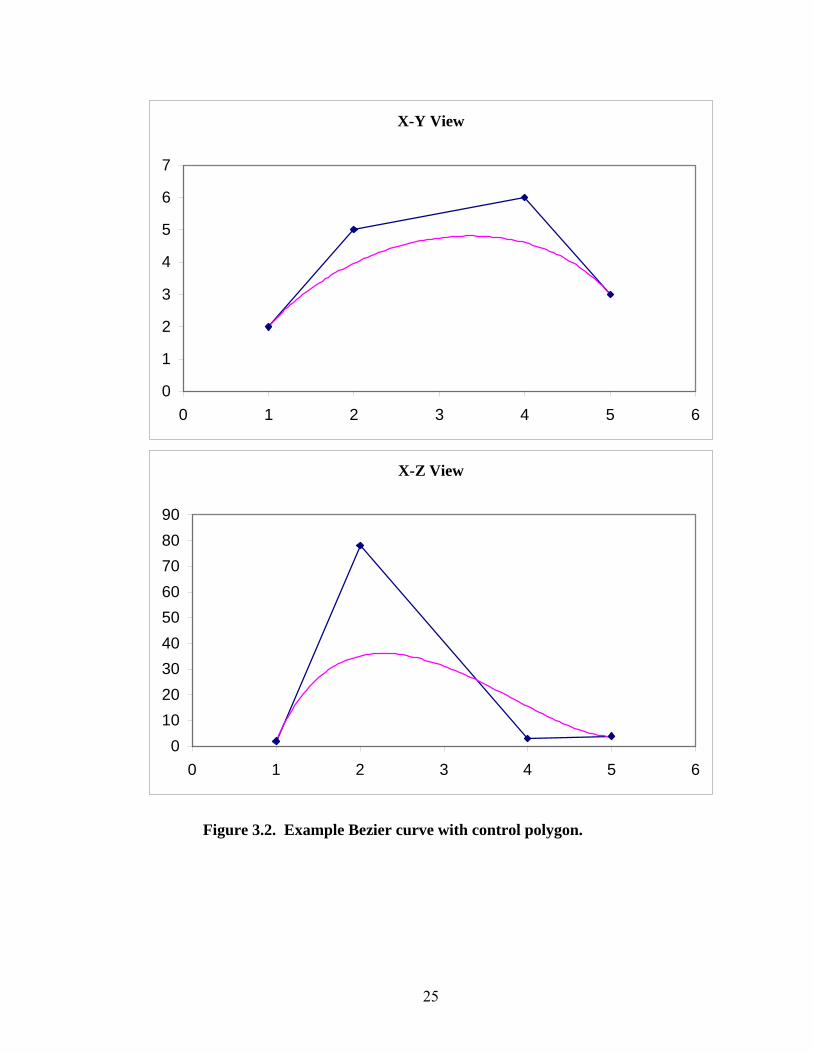
25
X-Y View
0
1
2
3
4
5
6
7
0 1 2 3 4 5 6
X-Z View
0102030405060708090
0 1 2 3 4 5 6
Figure 3.2. Example Bezier curve with control polygon.

26
In digital motion control, points along a path are specified at discrete time intervals. To
specify a point Pi on a parametric curve P(u) such as a NURBS or Bezier, an appropriate
parameter value ui must be chosen that matches the desired length along the curve Si. To
do this, the relationship (3.3) between the parameter value u and the length S(u) along the
curve must be resolved.
( )∫ ′=uu0
duuS)u(S (3.3)
Since (3.3) cannot be solved in closed form, ui cannot be calculated exactly without
resorting to iterative methods. Due to the real-time nature of machine control, calculation
time must be made deterministic by avoiding iterative methods, but errors in ui will
negatively affect motion dynamics and must be controlled. These effects can be kept
within acceptable levels if the controller can specify the maximum length error εlength,
where
iilength S)u(S −≥ε (3.4)
To do this, some iteration will be necessary, so to satisfy the requirements of real-time
control, a method with rapid convergence must be used.
Previous efforts to tackle this problem [2, 11-13, 30, 32, 35, 37-39, 42] yielded
algorithms that are either nonlinearly extrapolative (and thus inherently unstable) or
highly iterative (such as first-derivative extrapolations and interval halving methods).

27
While the latter may seem attractive at first due to the simplicity and speed of such
algorithms, their overall calculation time can quickly surpass that of more complicated
methods since (3.3) must be evaluated as part of every iteration and checked against
(3.4).
3.2 METHOD
To develop a stable, fast algorithm that minimizes iteration, this thesis uses modified
versions of [12] and [38]. A basic predictor-corrector algorithm, such as is found in [38]
is outlined in Fig. 3.3. First, the curve is initialized and a lookup table for the parameter-
length relationship is populated. When a length command comes down, a prediction is
made for the corresponding parameter. A length check is performed to confirm the
accuracy of the parameter. If the parameter does not hold the required tolerance, a
correction operation is performed. The check and correction are repeated until the
tolerance or some other criterion is met, such as a limit on the number of iterations. Then
the parameter is passed on and is used to establish the next waypoint.
The same basic approach Fig. 3.3 will be used in this method to calculate the parameter.
The remainder of this chapter develops improved prediction and correction steps.
Section 3.2.1 reviews the Length Calculation method of Günter and Parent [12]. Section
3.2.2 outlines a method of establishing a lookup table for the parameter-length
relationship, which will be used in the prediction and correction steps. Section 3.2.3
presents an interpolative prediction method using a monotonic curve scheme. Section
3.2.4 gives a simple method for reducing the parameter error to an acceptable level.

28
3.2.1 LENGTH CALCULATION
The first thing a predictor-corrector needs is a reliable way to calculate the length along a
curve (the arc length) at a parameter value. This is done by integrating (3.3). Günter and
Parent [12] developed such a method using a lookup table and Gauss-Legendre
quadrature, and the method was clarified by Yang and Red [38], which also added an
error analysis. This method is reviewed here, with minor changes.
Figure 3.3. Typical predictor-corrector algorithm.
No
Yes
Initialization Lookup table generation
Desired Length
Length Calculation
Parameter Finalized Waypoint calculated Other Calculations
Parameter Prediction
Length tolerance met?
Parameter Correction
Max. number of iterations?
Yes
No

29
Gauss-Legendre quadrature is a numerical method of integration that is exact for
polynomials of degree ≤ (2n-1), where n is the degree of the quadrature. Gauss-Legendre
quadrature integrates a function by summing weighted evaluations of that function. If the
function S’(u) is to be integrated over an arbitrary interval u=[a,b], the quadrature
equation is
( ) ( ) ( )∑∫=
′ε+′=′n
0iii
ba
b,a,n,SuSwduuS (3.5)
where ε( S’,n,a,b) is the error function and wi are tabulated weights. From Kythe and
Schaeferkotter [19]:
( ) ( )
2abxabu i
i++−
= (3.6)
( ) ( ) ( )( )ξ−=′ε ++ 1n2n
1n2 SKabb,a,n,S (3.7)
where ( )b,a∈ξ ,
( )( ) ( )[ ]3
41n2n
!n21n2!n2K
+=
+ (3.8)

30
and xi and wi are tabulated constants that depend on the degree of the quadrature. These
constants can be found in most texts that deal with Gaussian quadrature, such as [19].
3.2.2 LOOKUP TABLE
The first thing that must be done in establishing a lookup table is to determine the number
of entries that are needed. The error function (3.7) can be used to do this.
The value S’max = max[S(2n+1)(ξ)] can be substituted into (3.7) to find the number of
divisions in the lookup table necessary to hold the length-calculation error:
( )
length
maxn1n2
tableSKab
Nε
′−=
+ (3.9)
Using Ntable (rounded up to the next largest integer) to calculate the parameter interval Δu
on which to set up the lookup table:
tableN
abu −=Δ (3.10)
A quadrature operation is performed on each interval to populate the “Length” column of
the lookup table, as in Table 3.2.

31
Subsequent length calculations are performed on a subinterval. For example, if a
parameter u is chosen such that ui < u < ui+1, then the quadrature operation will be
performed on the interval [ui, u] and the result added to Si.
Node Parameter Length
0 a 0
1 u1 S1
... ... ...
Ntable-1 uNtable-1 SNtable-1
Ntable b SNtable = S(b)
3.2.3 PARAMETER PREDICTION
With a lookup table established, a method must be defined to predict a parameter u given
a desired length S. Some predictors use a first- or second-order Taylor expansion or a
tangent magnitude method of prediction. Other papers use polynomial predictors based
upon previous waypoints. Yang and Red [38] used Lagrange interpolation over previous
waypoints to predict the next waypoint parameter. Second-order expansions and
polynomial predictors have the disadvantage of doubling back, i.e. they can reach a point
where an increase in length results in a decrease in parameter, as in Fig. 1.4. This is not
representative of the monotonic nature of (3.3) and can easily defeat the prediction
scheme. First-order and tangent magnitude methods may suffer from low convergence
rates. All current methods in the literature are extrapolative.
Table 3.2. Lookup table for parameter-length relationship.

32
The current methods in the literature usually work for step sizes that are small in relation
to the length of the curve. However, as the step sizes increase, the extrapolations break
down. A prediction method will now be presented that is both interpolative and
representative of the monotonic nature of (3.3). This method is stable and will provide
better convergence rates for larger step sizes.
Sarfraz [27] developed a curve definition with specifiable endpoints and derivatives.
This curve is guaranteed to be monotonic. An interpolative prediction method using a
monotonic curve with specifiable end conditions will generally follow the length curve
better than extrapolative polynomial and derivative methods, as illustrated in Fig. 3.4.
The Sarfraz curve is a rational cubic spline that is guaranteed to be monotonic. While the
curve is presented in [27] as a spline, for clarity it will be defined here as an individual
curve segment (3.12). Some minor simplifications are also made that result from the
constraints of the present application. Given endpoints (S0, u0), (S1, u1) and derivatives d0
and d1 where
( )ii uS
1d′
= (3.11)
the Sarfraz curve is defined as

33
( ) ( )( ) [ ]( ) ( ) [ ]( )
( ) ( ) ( ) 322310101
201001
210
111
dSSuu1uudSS1
u1uSu
θ+θ−ωθ+θ−ωθ+θ−
−−−θ−θ++−−θ−θ+
θ+θ−=
(3.12)
01
0SSSS
−−
=θ (3.13)
( )( )01
0101uu
SSdd−
−+=ω (3.14)
The monotonicity of this curve is proven in [27].
0.25
0.29
0.33
0.37
0.41
0.45
33.5 34 34.5 35 35.5 36
Length
Para
met
er
Length CurveLookup TableLagrange PointsLagrange CurveSarfraz Curve
Figure 3.4. Comparison of Lagrange curve and monotonic Sarfraz curve for parameter prediction.

34
To predict a parameter value, the lookup table is searched to find the interval on which
the desired length resides. Using the endpoints of this interval and the corresponding
derivatives, a Sarfraz curve segment is set up over the interval. Evaluating the Sarfraz
curve at the desired length yields a parameter prediction. The actual length along the
curve at the predicted parameter can be obtained by performing a quadrature operation
from the beginning of the interval to the predicted parameter.
3.2.4 PARAMETER CORRECTION
The predicted parameter may violate the length tolerance εlength. In this case a correction
operation must be performed on the predicted parameter. This is easily done by setting
up another Sarfraz curve. If the predicted parameter is too high, the new Sarfraz curve is
set up between the beginning of the table interval and the predicted parameter. If the
predicted parameter is too low, the new Sarfraz curve is set up between the predicted
parameter and the end of the table interval. The new parameter is then predicted. If
necessary, another Sarfraz curve can be set up for another prediction. If this method is
combined with simple interval halving, the convergence rate is very rapid. The method is
also algorithmically stable.

35
4 METHOD: SPEED PROFILING
This chapter presents a method for planning the speed along a curve. Planning speed is
important for generating smooth accelerations and decelerations and for respecting
dynamic limitations on the machine and the manufacturing process.
Section 4.1 presents the definition of a simple jerk-limited speed profile. Section 4.2
explains the dynamic limitations a set of moves places on the speed profile. Section 4.3
defines a speed profiling algorithm that meets the requirements of real-time control.
4.1 THE JERK-LIMITED SPEED PROFILE
In machining operations, a desired tool tip speed is specified for any particular portion of
the process plan. However, each machine has its own dynamic limitations, so the tool
cannot always be moved at the desired speed along the entire path. Thus, the controller’s
job is to control the tool as close to the desired speed as possible while respecting
machine limitations. This is accomplished by the proper construction and following of
speed profiles. A speed profile is a map of the speed across an individual move or set of
moves.
Trapezoidal profiles used to be the norm in machine control. Over time the jerk
capabilities of motors advanced to the point where they began to stress mechanisms,

36
causing premature wear. Jerk is the time derivative of acceleration and can be thought of
as a measure of impact. Jerk-limited speed profiles were developed to reduce these
stresses. A typical jerk-limited speed profile section and its derivatives are defined by the
following time-dependent equations
( )6tJ
2tAtVStS
30
2start
startstart +++= (4.1)
( )2tJtAVtV2
0startstart ++= (4.2)
( ) tJAtA 0start += (4.3)
( ) 0JtJ = (4.4)
Note that if J0 = Jmax, the speed profile allows for the optimal (shortest) transition time
between speeds. Therefore, the maximum allowable jerk is always used.
Jerk-limited speed profiles consist of seven types of profile sections, classified by their
shape and behavior. These types are listed below and represented in Fig. 4.1.
1) Concave Rise
2) Linear Rise
3) Convex Rise

37
4) Constant Speed
5) Convex Fall
6) Linear Fall
7) Concave Fall
Speed Profile
0
9
0 0.5 1 1.5 2 2.5
Time
Spee
d
Setting up speed profiles of this nature is relatively straightforward using algorithms
currently found in the literature (Red [24], Erkorkmaz and Altintas [8], Nam and Yang
[22]). A more difficult problem is maintaining the desired speed while handling
sequential moves of all sizes and dynamic requirements. Indeed, defining the logic
necessary to create a robust speed profiler is a much more rigorous task than defining the
mathematics for individual profile segments. The specifics of the problem are explained
in Sections 4.2 and 4.3. A solution to the problem is given in Section 4.3.
1
2
3 4 5
6 7
Figure 4.1. The seven types of speed profile sections.

38
4.2 DYNAMIC LIMITATIONS ON SPEED PROFILES
Every move has its own dynamic limitations. In other words, each move interacts with
the machine differently so as to limit the feasible speed, acceleration, and jerk across that
move. A simple example is found in traversing a circular path at constant speed. Here,
the radial acceleration Ar depends on the traversal speed V and the radius of curvature R
of the path as
R
VA2
r = (4.5)
If there is a maximum allowable value for Ar, then it can be seen by inspection that the
value of R will have an effect on the allowable values of V.
A sequence of moves may have allowable speeds resembling the contrived example in
Fig. 4.2, but in the general case can take on essentially any shape. In addition to limited
speed, each move will have its own limits on allowable acceleration and jerk. The
calculation of these limits is discussed in Chapter 5. Since the current chapter is strictly
concerned with the construction of speed profiles, it is assumed that these limits have
already been calculated.
4.3 SPEED PROFILE CONSTRUCTION
Fig 4.2 shows an example of allowable (solid lines) and desired (dashed line) speeds for a
set of moves. It is important to realize that the allowable speeds for one move are
completely independent of every other move. Therefore the allowable speed plot can

39
assume any configuration. A speed profiler must be able to handle any set of moves, and
perform well. The problem is to construct such a speed profile over a given set of moves.
The requirements are as follows:
1) Increase as quickly as possible to the desired speed
2) Maintain as close a speed as possible to the desired speed
3) Respect the allowable speeds, accels, and jerks
4) Reach zero speed by the end of the last available move
Requirements 3 and 4 are of particular interest. Many published algorithms use
estimations of remaining length to plan their speed profiles or ignore this requirement
altogether, but if the speed profile is calculated incorrectly, so that zero speed profile does
not reach zero speed by the end of the move sequence, dynamic limitations will be
Figure 4.2. Example of allowable and desired speeds.
V
S

40
exceeded. Additionally, most papers ignore dynamics in order to simplify the algorithms.
These requirements, however, cannot be ignored in a real implementation.
In order to make the logic and accompanying explanation feasible, some simplifying
constraints will be applied to the speed profiling problem. That is, zero acceleration will
be specified at the endpoints of moves. This allows convergence to be guaranteed for the
algorithm, without iteration. Additionally, once the waypoint enters a segment, the speed
profile for that segment will not be adjusted.
The reader may assume that (referring to Fig. 4.1) accelerating profiles consist of a
sequence of profile segments of types 1 and 3 and that decelerating profiles consist of
profile segments of types 5 and 7. In other words, the explanations in this chapter refer to
speed profiles containing “perfect S-curves”, which do not contain portions of constant
acceleration or constant speed. The logic for using speed profiles with constant
acceleration or constant speed portions is similar to that for perfect S-curves. Including
speed profiles with constant acceleration or speed would unnecessarily multiply the
number of cases that need to be explained. Thus, in order to facilitate reader
understanding of the underlying speed profiling concept, the specific cases for profiles
including constant acceleration and speed portions are not discussed.
The algorithm comes in two parts, a forward recursion and a backward recursion,
explained in detail in Sections 4.3.1 and 4.3.2. The purpose of the forward recursion is to
attain and maintain the specified speed. The backward recursion ensures that allowable

41
speeds are respected and that the speed profile can reach zero before the end of the move
sequence. The backward recursion is only needed if the forward recursion fails to
generate a feasible profile.
The logic for the forward and backward recursions are given in Sections 4.3.1 and 4.3.2,
respectively. A pseudocode summary of the speed profiling algorithm is given in Section
4.3.3. A peculiarity of s-curve speed profiles is that the profile may have a “dead spot,” a
range of speed that cannot be reached with the specified acceleration and jerk. A
mathematical explanation for this is given in Section 4.3.4.
4.3.1 FORWARD RECURSION
The forward recursion attempts to reach the desired speed by accelerating over one or
more upcoming move segments. It then attempts to reach zero speed by decelerating
over the remaining segments. This process is shown in Fig. 4.3. Each time the waypoint
enters a new move segment, the speed profiler attempts to increase speed over the
following move (optionally, several upcoming moves), and then decreases to zero. This
also happens on the first step after starting from zero, as in Fig. 4.4. In this way, the
speed profile is always increasing, but only over the minimum number of segments
necessary. This allows the profile to define a path to zero speed with as little calculation
time as possible. In both Figs. 4.3 and 4.4 the ‘X’ indicates the current position in the
speed profile.

42
There are a number of cases that arise during the forward recursion. These cases and the
logic for handling them are presented in Section 4.3.1.1 for the acceleration stage and
Section 4.3.1.2 for the deceleration stage.
Figure 4.3. Example forward recursion beginning from zero speed.
V
S
V
S
V
S
V
S

43
4.3.1.1 ACCELERATION STAGE
In the acceleration stage, the speed profiler attempts to reach the desired speed by
increasing speed over a segment of known length. If it is necessary to decrease speed
over that segment to maintain allowable speeds, the profiler tries to hold the highest
Figure 4.4. Example forward recursion upon stepping into a new move segment.
V
S
V
S
V
S
V
S
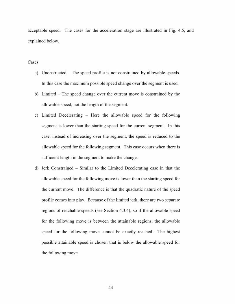
44
acceptable speed. The cases for the acceleration stage are illustrated in Fig. 4.5, and
explained below.
Cases:
a) Unobstructed – The speed profile is not constrained by allowable speeds.
In this case the maximum possible speed change over the segment is used.
b) Limited – The speed change over the current move is constrained by the
allowable speed, not the length of the segment.
c) Limited Decelerating – Here the allowable speed for the following
segment is lower than the starting speed for the current segment. In this
case, instead of increasing over the segment, the speed is reduced to the
allowable speed for the following segment. This case occurs when there is
sufficient length in the segment to make the change.
d) Jerk Constrained – Similar to the Limited Decelerating case in that the
allowable speed for the following move is lower than the starting speed for
the current move. The difference is that the quadratic nature of the speed
profile comes into play. Because of the limited jerk, there are two separate
regions of reachable speeds (see Section 4.3.4), so if the allowable speed
for the following move is between the attainable regions, the allowable
speed for the following move cannot be exactly reached. The highest
possible attainable speed is chosen that is below the allowable speed for
the following move.

45
e) Violating – The allowable speed for the following move will be violated.
Here the starting speed for the following move is set to the allowable
speed and a backward recursion must be performed.
f) End of Buffer – Zero speed could not be reached by the end of the last
segment. The ending speed of that segment is set to zero and a backward
recursion is begun.
4.3.1.2 DECELERATION STAGE
The deceleration stage is much simpler than the acceleration stage. Here the speed
profiler simply tries to decrease to zero speed as fast as possible. The cases for the
deceleration stage are found in Fig. 4.6, and explained below.
Cases:
a) Unobstructed – The speed profile is not constrained by allowable speeds.
In this case the maximum possible speed change over the segment is used.
b) Violating – The allowable speed for the following move will be violated.
Here the starting speed for the following move is set to the allowable
speed and a backward recursion must be performed.
c) End of Buffer – Zero speed could not be reached by the end of the last
segment. The ending speed of that segment is set to zero and a backward
recursion is begun.
d) Stopped – The speed profile has reached zero speed.

46
4.3.2 BACKWARD RECURSION
The backward recursion attempts to construct a feasible speed profile when the forward
recursion fails, such as when an allowable speed violation occurs (Fig. 4.7). The
backward recursion begins where the forward recursion ended, at zero speed. It then
constructs a speed profile in the reverse direction, always trying to “connect” with the
speed profile currently in use.
Figure 4.6. Forward recursion, deceleration stage cases.
c V
S
b V
S
a V
S
d V
S

47
There are two main cases that arise during the backward recursion, the case when the
motion is starting from zero and a speed profile is not yet established, and the case when
the motion is already moving on a speed profile and the motion planner is attempting to
construct a new speed profile. These cases and the logic for handling them are presented
in Section 4.3.2.1 for the case where a current speed profile is established and Section
4.3.2.2 for the case where there is no current speed profile in use.
4.3.2.1 PROFILE ESTABLISHED
If a useable speed profile has already been established, the goal of the backward
recursion is to connect with that speed profile. The cases encountered are shown in Fig.
4.8, and explained below.
Figure 4.7. Example of a failed forward recursion.
V
S

48
Cases:
a) Converged Increasing – The backward recursion converges with the
established speed profile.
b) Jerk Limited – The backward recursion can reach above and below the
established speed profile but cannot converge with it. Here the higher
speed will be kept.
Figure 4.8. Backward recursion cases with profile established.
d V
S
a V
S
b V
S
c V
S

49
c) Decreasing – The backward recursion tries to converge with the
established speed profile by decreasing speed but cannot converge. The
lowest attainable speed is kept.
d) Converged Decreasing – The backward recursion converges with the
established speed profile by decreasing speed.
4.3.2.2 NO PROFILE ESTABLISHED
If no useable speed profile has been established, the goal of the backward recursion is to
connect with the forward recursion. Because the forward recursion can have
discontinuities, if the backward recursion converges with the forward recursion, the
backward recursion will still construct a full profile back to the beginning of the buffer.
The cases encountered are shown in Fig. 4.9, and explained below.
Cases:
a) Nonconverged – The backward recursion does not converge with the
forward recursion. In this case the highest attainable speed is kept.
b) Converged – The backward recursion can converge with the forward
recursion. The backward recursion is continued, always trying to follow
the forward recursion.
c) First Segment – The backward recursion reaches the first segment and
decreases to zero.

50
4.3.3 ALGORITHM SUMMARY
Presented below is a pseudocode summary of the speed profiling algorithm.
//begin forward recursion //begin acceleration phase if Current speed is zero start on current segment else start on segment after the current segment Test for the highest attainable speed if allowable speed is lower than the attainable speed keep the allowable speed else
Figure 4.9. Backward recursion cases with no profile established.
b V
S
a V
S
c V
S

51
keep the attainable speed move to next segment //begin deceleration phase loop test for the lowest attainable speed if attainable speed is less than or equal to zero keep zero as the speed exit forward recursion else if end of buffer is reached keep zero as the speed must do a backward recursion exit forward recursion else if allowable speed is lower than the attainable speed keep the allowable speed must do a backward recursion else keep the attainable speed move to next segment //begin backward recursion if must do backward recursion Start at end of forward recursion loop if at current segment try to link with current segment starting speed if successful use backward recursion as the useable profile exit backward recursion else discard backward recursion exit backward recursion if No useable profile Test for the attainable speed if we can attain same or higher speed than the forward
recursion if the forward recursion is lower than the current ending state
find the low speed we can attain if we can reach down to the forward recursion keep the forward recursion value
else keep the lower attainable speed else keep the forward recursion value else keep the attainable speed else Test for the attainable speed if we can attain same or higher speed than the useable profile if useable profile is higher than the current ending state use the rest of the useable profile else find the lowest attainable speed if we can reach the useable profile or lower if we can reach the exact value of the useable profile use the rest of the useable profile else
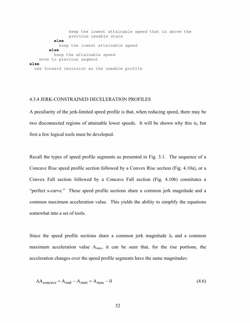
52
keep the lowest attainable speed that is above the previous useable state
else keep the lowest attainable speed else keep the attainable speed move to previous segment else use forward recursion as the useable profile
4.3.4 JERK-CONSTRAINED DECELERATION PROFILES
A peculiarity of the jerk-limited speed profile is that, when reducing speed, there may be
two disconnected regions of attainable lower speeds. It will be shown why this is, but
first a few logical tools must be developed.
Recall the types of speed profile segments as presented in Fig. 3.1. The sequence of a
Concave Rise speed profile section followed by a Convex Rise section (Fig. 4.10a), or a
Convex Fall section followed by a Concave Fall section (Fig. 4.10b) constitutes a
“perfect s-curve.” These speed profile sections share a common jerk magnitude and a
common maximum acceleration value. This yields the ability to simplify the equations
somewhat into a set of tools.
Since the speed profile sections share a common jerk magnitude J0 and a common
maximum acceleration value Amax, it can be seen that, for the rise portions, the
acceleration changes over the speed profile segments have the same magnitudes:
0AAAA maxstartendconcave −=−=Δ (4.6)

53
maxstartendconvex A0AAA −==Δ − (4.7)
Dividing by their respective jerks it can be seen that
0maxconvex0maxconcave J/AtJ/At −−=Δ==Δ (4.8)
So the total time for the speed change is
0max J/A2T = (4.9)
Plugging this into (4.2) and subtracting starting velocities yields
Figure 4.10. Perfect s-curve speed profiles.
b V
t
a V
t

54
0
2max
convexconcave J2AVV =Δ=Δ (4.10)
so
0
2max
rise JAV =Δ (4.11)
Plugging T into (4.1) and subtracting starting length yields
20
3max
0
maxstartconcave
J3A2
JAVS +=Δ (4.12)
( )
20
3max
0
maxrisestartconvex
J3A
J2AVV2S +
Δ+=Δ (4.13)
20
3max
0
maxstartrise
JA
JAV2S +=Δ (4.14)
where J0 is equal to the maximum jerk for the move segment and ΔS is equal to the length
of the move segment.
Similarly, for the fall portion
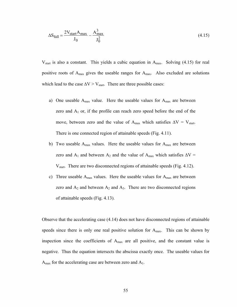
55
20
3max
0
maxstartfall
JA
JAV2S −=Δ (4.15)
Vstart is also a constant. This yields a cubic equation in Amax. Solving (4.15) for real
positive roots of Amax gives the useable ranges for Amax. Also excluded are solutions
which lead to the case ΔV > Vstart. There are three possible cases:
a) One useable Amax value. Here the useable values for Amax are between
zero and A1 or, if the profile can reach zero speed before the end of the
move, between zero and the value of Amax which satisfies ΔV = Vstart.
There is one connected region of attainable speeds (Fig. 4.11).
b) Two useable Amax values. Here the useable values for Amax are between
zero and A1 and between A2 and the value of Amax which satisfies ΔV =
Vstart. There are two disconnected regions of attainable speeds (Fig. 4.12).
c) Three useable Amax values. Here the useable values for Amax are between
zero and A2 and between A2 and A3. There are two disconnected regions
of attainable speeds (Fig. 4.13).
Observe that the accelerating case (4.14) does not have disconnected regions of attainable
speeds since there is only one real positive solution for Amax. This can be shown by
inspection since the coefficients of Amax are all positive, and the constant value is
negative. Thus the equation intersects the abscissa exactly once. The useable values for
Amax for the accelerating case are between zero and A1.

56
Figure 4.11. Illustration of attainable speed region for 1 useable Amax value.
Amax = A1
Amax = 0
Attainable Speeds
V
t
Figure 4.12. Illustration of attainable speed region for 2 useable Amax values.
Amax = A1
Amax = 0
Attainable Speeds
Amax = A2
V
t

57
Figure 4.13. Illustration of attainable speed region for 3 useable Amax values.
Amax = A1
Amax = 0
Attainable Speeds
Amax = A2
Amax = A3
V
t

58

59
5 METHOD: DYNAMICS
There are two types of dynamic limitations that arise in machining operations: process
limitations and machine limitations. Process limitations are machine independent and
relate only to motion along the path and interactions between the tool and the workpiece.
For example, forces on a cutting tool depend upon the speed, acceleration, and jerk at
which the tool is moved through material. Machine limitations apply to each joint of the
machine tool and depend upon both the shape of the path and the motion along the path
as defined by the speed profile. Due to this relationship, the path dynamics (speed,
acceleration, jerk) that will give acceptable joint dynamics must be determined.
This chapter will outline a method for determining the allowable path dynamics for
moves. The allowable values for path dynamics can then be used by the speed profiler in
Chapter 4 to develop feasible speed profiles. Section 5.1 presents the mathematical
relationship between motion along curves in path space and motion in joint space.
Section 5.2 gives a quick overview of the variation diminishing property of Bezier
curves. Section 5.3 presents a heuristic method for determining allowable speeds based
on the variation diminishing property.

60
5.1 PATH-JOINT RELATIONSHIPS
A Bezier path is described by the equation
( ) ( )( )∑
==
n
0inii
niiiuBvuBvu PP (5.1)
where
[ ]Tiziyixi PPP=P (5.2)
are points in Cartesian space,
( ) ( ) inini u1u
in
uB −−⎟⎟⎠
⎞⎜⎜⎝
⎛= (5.3)
are Bernstein polynomials,
( ) !i!in!n
in
−=⎟⎟
⎠
⎞⎜⎜⎝
⎛ (5.4)
is the binomial coefficient, and vi are positive definite weighting values.
Section 5.1.1 presents the equations for relating a curve and its parametric derivatives in
path space to joint space. Section 5.1.2 presents the relations for derivatives with respect
to arc length. Section 5.1.3 presents the relations for derivatives with respect to time.

61
5.1.1 PARAMETRIC DERIVATIVES
For 3-degree-of-freedom machines, such as those in Fig. 5.1, points in path space P can
be related to points in joint space q by use of a machine-specific inverse kinematics
transformation K, so that
( ) ( )( )uu PKq = (5.5)
where
( )( )
( )⎥⎥⎥
⎦
⎤
⎢⎢⎢
⎣
⎡=
P
PPK
m
1
q
qM (5.6)
While the inverse kinematics transformations for 3-axis mechanisms are relatively
simple, the relationship between path dynamics and joint dynamics are a bit more
complicated. These dynamics must be kept in check to ensure smooth motion along the
path and stay within the capabilities of the machine.
Parametric relationships for joint dynamics can be found by taking the derivatives of
(5.5):
( ) ( )( )PPKq ′=′ udu (5.7)
where

62
( )( )
( )
( ) ( ) ( )
( ) ( ) ( )( )j
i
z
m
y
m
x
m
z
1
y
1
x
1
m
1
Pq
Pq
Pq
Pq
Pq
Pq
Pq
dq
dqd
∂∂
=
⎥⎥⎥⎥⎥⎥
⎦
⎤
⎢⎢⎢⎢⎢⎢
⎣
⎡
∂∂
∂∂
∂∂
∂∂
∂∂
∂∂
=⎥⎥⎥
⎦
⎤
⎢⎢⎢
⎣
⎡=
PPPP
PPP
P
PPK MMMM (5.8)
Similarly,
( ) ( )( )( )( )( ) ( )( )PPKPPPKq ′′+′′=′′ ududu 2 (5.9)
Figure 5.1. Some simple 3-axis mechanisms. a) Rectangular mechanism. b) Cylindrical mechanism.
x y
z z
φ
r
a) b)

63
( ) ( )( )( )( )( )( )( ) ( )( )( )( )( ) ( )( )PPKPPPKPPPPKq ′′′+′′′+′′′=′′′ udud3udu 23 (5.10)
where
( ) ( )kj
i2
2PP
qd∂∂
∂=
PPK (a 3-dimensional tensor) (5.11)
( ) ( )lkj
i3
3PPP
qd∂∂∂
∂=
PPK (a 4-dimensional tensor) (5.12)
5.1.2 ARC-LENGTH DERIVATIVES
Using the parametric joint derivatives, the derivatives with respect to arc-length can be
calculated.
( ) ( ) ( ) SS uudS
udu qqq ′== (5.13)
where
( )u1uS q′
= (5.14)
and

64
( ) ( ) ( )du
duuuuuu s
S2SSS qqq ′+′′= (5.15)
( ) ( ) ( ) ( )⎟⎟
⎠
⎞
⎜⎜
⎝
⎛+⎟
⎠⎞
⎜⎝⎛′+′′+′′′= 2
S2
2S
2S
SS2
S3SSSS
duudu
duduuu
duduuu3uuu qqqq (5.16)
5.1.3 TIME DERIVATIVES
The time derivatives are calculated from the arc-length derivatives as follows:
( ) ( ) ( )dtdSu
dtudu Sqqq ==& (5.17)
Note that the final term in (5.17) is simply a speed term, so (5.17) can be written a little
more clearly as
( ) ( )Vuu Sqq =& (5.18)
Continuing with the next two derivatives,
( ) ( ) ( )AuVuu S2
SS qqq +=&& (5.19)
( ) ( ) ( ) ( )JuAVu3Vuu SSS3
SSS qqqq ++=&&& (5.20)

65
Equations 5.18 - 5.20 map the relationship between the path dynamics and joint
dynamics. The left-hand terms are the machine joint dynamics and are known. Inserting
their maximum values and inverting the equations yields a method for calculating the
allowable path dynamics:
( )VminVmax = (5.21)
where
( )( )uu
SqqV&
= (5.22)
and the division of two vectors is a component-wise division.
Likewise,
( )AminAmax = (5.23)
( ) ( )( )u
Vuu
S
2SS
qqqA
−=&&
maxmax VVV ≤≤− (5.24)
( )JminJmax = (5.25)
66
( ) ( ) ( )
( )uAVu3Vuu
S
SS3
SSSq
qqqJ −−=
&&& (5.26)
where
maxmax VVV ≤≤−
and
maxmax AAA ≤≤− .
Calculating the extrema of these dynamic equations is expensive. Fortunately, the
variation diminishing property (Section 5.2) of Bezier curves and a bit of heuristics can
be used to make the job easier.
5.2 VARIATION DIMINISHING
The variation diminishing property of Beziers is that a line (for planar Beziers) or a plane
(for 3D Beziers) will not intersect the curve more times than it intersects the control
polygon. The physical meaning of this is that the curve will not “wiggle” more than the
control polygon. This is illustrated in Fig. 5.2, where a variety of lines (dashed) are
intersecting a Bezier curve and its control polygon. The solid line represents the Bezier
curve. The dotted line represents the control polygon.

67
5.3 SAMPLING METHOD
Since the curve cannot wiggle more times than its control polygon, the variation of its
shape is limited. If the curve is sampled at an appropriate interval, say Δu = 0.1, this
variation will be evident. Fig. 5.3 gives an illustration of what such a sampling scheme
would appear like when applied to a Bezier curve.
In addition to revealing the shape of a curve, the sampling method can be applied to the
dynamic equations (5.22, 5.24, 5.26). A good approximation of the dynamics can be
extracted by analyzing the dynamics equations at each of the sample points. From that a
set of points on the curve is determined at which we know the limits on path dynamics.
This information can be used in a number of ways. In this thesis, the simplest method is
Figure 5.2. Illustration of variation diminishing property.

68
used, where the most conservative of the path dynamics is chosen and applied to the
entire curve segment.
Figure 5.3. Illustration of sampling method.

69
6 RESULTS & DISCUSSION
This chapter presents the results of the methods developed in this thesis. The methods
were tested under real-world conditions. The results are taken from the milling of the
automotive surface shown in Fig. 6.1. The milling was done at BYU on a Tarus styling
mill similar to the one shown in Fig. 6.2. Tool paths were generated using Unigraphics
NX 2.0.
Section 6.1 presents the results of the Predictor-Corrector module for calculating
appropriate parameter values. Section 6.2 gives the results of the Speed Profiling and
Dynamics modules. Section 6.3 presents the machined part. Section 6.4 summarizes the
results.
Figure 6.1. Automotive surfaces used for test.
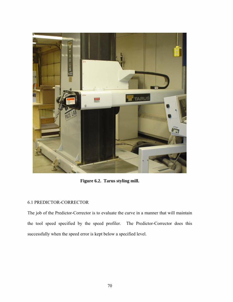
70
6.1 PREDICTOR-CORRECTOR
The job of the Predictor-Corrector is to evaluate the curve in a manner that will maintain
the tool speed specified by the speed profiler. The Predictor-Corrector does this
successfully when the speed error is kept below a specified level.
Figure 6.2. Tarus styling mill.

71
Fig. 6.3 shows a line plot of the speed error for the Predictor-Corrector for each step,
normalized to the specified maximum error fraction of 1E-6. Note that all values are
below one. Thus the specified error fraction is being held by the Predictor-Corrector.
6.2 SPEED PROFILING AND MOTION DYNAMICS
The Motion Dynamics module analyzes each curve and decides the maximum allowable
path speeds, accels, and jerks along that curve based on dynamic joint limitations and
chordal error. The speed profiler keeps the speed as close to the desired speed as possible
without violating motion dynamics.
Figure 6.3. Predictor-Corrector error fraction for each step, normalized to the maximum allowable error fraction.

72
The Speed Profiling and Motion Dynamics modules are closely related, so they are both
evaluated at the same time.
Section 6.2.1 specifically evaluates the accuracy of the Speed Profiling module by
examining the tool speed along the path. Section 6.2.2 analyzes the chordal error
generated by the motion along the curve. Section 6.2.3 analyzes the dynamics of motion
of each of the joints on the Tarus mill.
6.2.1 TOOL SPEED
The allowable speed is decided by the Motion Dynamics module and is different for each
curve section. Fig 6.4 shows a line plot of the tool speed at each step, normalized to the
allowable speed. All values are at or below one. This means that the allowable speed
settings are being obeyed by the Speed Profiler.
It is interesting to note that, due to dynamic limitations, the speed profiler is not always
able to hold the desired speed. This does not mean that the speed profiler is failing,
simply that it is reducing speed at certain points in order to obey dynamic limitations.
Fig. 6.5 shows a line plot of the actual tool speed at each step, normalized to the desired
speed of 80 mm/s.

73
Figure 6.4. Tool speed, normalized to the allowable speed for each curve segment.
Figure 6.5. Tool speed, normalized to desired speed.

74
Figs. 6.6 to 6.18 show the behavior of the speed profiler at a more localized level. Fig.
6.6 shows the speed profile for the first sixteen seconds of the process plan. The actual
tool speed is shown in blue, the commanded tool speed in green, and the maximum
allowable tool speed for each move is shown in red. Fig. 6.7 shows the speed profile for
the first four seconds of the process plan, with the same color scheme as in Fig. 6.6. Figs.
6.8 and 6.9 show the corresponding path acceleration and jerk profiles, respectively, with
the actual value shown in blue and the allowable values shown in red and green. Note
that the speed profiler attempts to reach and maintain the desired speed while respecting
the maximum allowable speed, acceleration, and jerk. For reference, Figs. 6.10 to 6.18
show the resulting dynamics effects on the individual axes.
Figure 6.6. Tool speed with commanded and maximum allowable speed for first sixteen seconds of the milling process.

75
Figure 6.7. Tool speed with commanded and maximum allowable speed for first four seconds of the milling process.
Figure 6.8. Tool acceleration with maximum allowable acceleration for first four seconds of the milling process.

76
Figure 6.9. Tool jerk with maximum allowable jerk for first four seconds of the milling process.
Figure 6.10. X axis velocity for first four seconds of the milling process.

77
Figure 6.11. Y axis velocity for first four seconds of the milling process.
Figure 6.12. Z axis velocity for first four seconds of the milling process.

78
Figure 6.13. X axis acceleration for first four seconds of the milling process.
Figure 6.14. Y axis acceleration for first four seconds of the milling process.

79
Figure 6.15. Z axis acceleration for first four seconds of the milling process.
Figure 6.16. X axis jerk for first four seconds of the milling process.

80
Figure 6.17. Y axis jerk for first four seconds of the milling process.
Figure 6.18. Z axis jerk for first four seconds of the milling process.

81
6.2.2 CHORDAL ERROR
Chordal error is the maximum distance between the curve geometry and the straight lines
generated by digital control. Fig. 6.19 shows a line plot of the maximum chordal error
for each step, normalized to the maximum allowable chordal error of 0.001 in. This plot
shows that the chordal error is not of much concern in the present process plan, as all
values are well below one.
Figure 6.19. Chordal error, normalized to maximum error tolerance.

82
6.2.3 MOTION DYNAMICS
The motion dynamics for each axis on the Tarus styling mill are shown in Sections
6.2.3.1 to 6.2.3.4. The line plots shown in these sections have been normalized to their
maximum allowable values. The maximum allowable values for each axis are shown in
Table 6.1.
AXIS Speed (mm/s) Accel (mm/s2) Jerk (mm/s3)
X 170 400 4000
Y 180 600 6000
Z 240 2000 20000 Section 6.2.3.1 gives the position plots for each axis. This is for reference purposes only.
Section 6.2.3.2 gives the normalized speed plots for each axis. Section 6.2.3.3 gives the
normalized speed acceleration plots for each axis. Section 6.2.3.4 gives the normalized
jerk plots for each axis. Section 6.2.3.5 presents an analysis of the dynamic plots.
6.2.3.1 AXIS POSITIONS
This section presents the position verses time for each axis of the Tarus styling mill.
These are provided for reference purposes and do not indicate the performance of the
algorithms in this thesis.
Table 6.1. Allowable axis dynamics for Tarus styling mill.

83
Figure 6.20. Dynamic position plot for X axis.
Figure 6.21. Dynamic position plot for Y axis.

84
6.2.3.2 NORMALIZED AXIS VELOCITIES
This section presents line plots of the normalized velocity verses time for each axis of the
Tarus styling mill. It can be observed that all the absolute values are less than unity and
thus the velocity limitations of each joint are being obeyed.
Figure 6.22. Dynamic position plot for Z axis.

85
Figure 6.23. Dynamic velocity plot for X axis.
Figure 6.24. Dynamic velocity plot for Y axis.

86
6.2.3.3 NORMALIZED AXIS ACCELERATIONS
This section presents line plots of the normalized acceleration verses time for each axis of
the Tarus styling mill. It can be observed that all the absolute values are less than unity
and thus the acceleration limitations of each joint are being obeyed.
Figure 6.25. Dynamic velocity plot for Z axis.

87
Figure 6.26. Dynamic acceleration plot for X axis.
Figure 6.27. Dynamic acceleration plot for Y axis.

88
6.2.3.4 NORMALIZED AXIS JERKS
This section presents line plots of the normalized jerk verses time for each axis of the
Tarus styling mill.
Figure 6.28. Dynamic acceleration plot for Z axis.

89
Figure 6.29. Dynamic jerk plot for X axis.
Figure 6.30. Dynamic jerk plot for Y axis.

90
6.2.3.5 ANALYSIS OF DYNAMICS
All the dynamic plots show joint dynamics kept within limits except for the Axis 2 jerk
plot (Fig. 6.30), which shows intermittent jerk violations of up to 40%.
Some of these high jerk values are caused by the transition from one NURBS curve to
another, where the ends of the curves are not curvature continuous. The smoothing of
such transitions is beyond the scope of this thesis. Removing the steps that include such
transitions yields a better picture of the performance of the algorithms in this thesis and
gives the plot in Fig. 6.32. This plot shows improved results, with most violations at
Figure 6.31. Dynamic jerk plot for Z axis.

91
around 10%, with occasional violations up to 25%. While there is room for
improvement, violations of this magnitude are of little concern. Jerk is extremely
sensitive to any perturbation, and disruptions of smooth motion typically show up as jerk
violations of several orders of magnitude.
6.3 MACHINED PART
Fig. 6.33 shows the automotive surface as machined. Visual inspection of the surface
indicates that the part was machined correctly and yields results comparable to traditional
machining methods.
Figure 6.32. Dynamic jerk plot for Y axis, transitions removed.
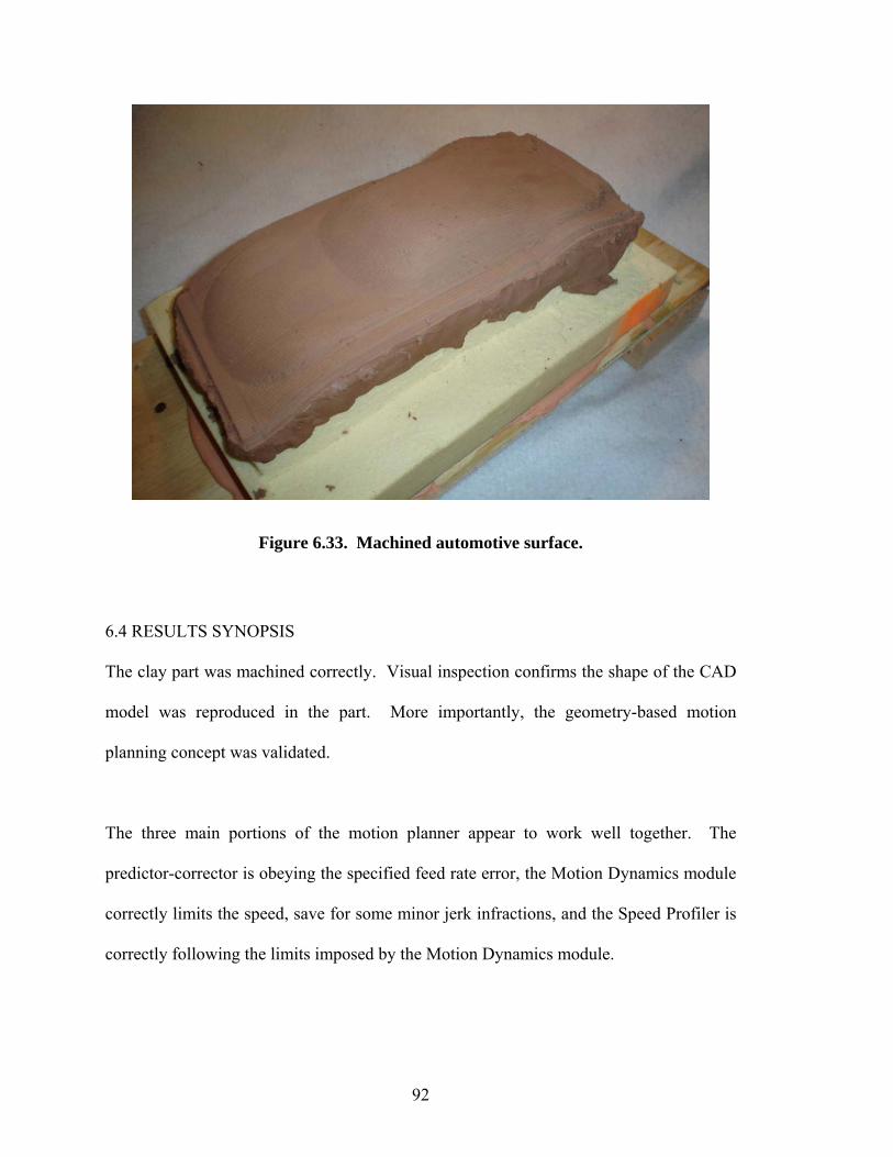
92
6.4 RESULTS SYNOPSIS
The clay part was machined correctly. Visual inspection confirms the shape of the CAD
model was reproduced in the part. More importantly, the geometry-based motion
planning concept was validated.
The three main portions of the motion planner appear to work well together. The
predictor-corrector is obeying the specified feed rate error, the Motion Dynamics module
correctly limits the speed, save for some minor jerk infractions, and the Speed Profiler is
correctly following the limits imposed by the Motion Dynamics module.
Figure 6.33. Machined automotive surface.

93
7 CONCLUSION AND RECOMMENDATIONS
This thesis has developed a working geometry-based parametric curve module for the
DMAC controller’s motion planner. This module allows for motion over parametric
polynomial curves such as Bezier and NURBS curves. The actual geometry provided by
the process planning software was used, providing for a parametric curve module that is
completely geometry-based. The four important aspects of motion: feed rate error, path
accuracy, motion dynamics, and speed profiling were successfully integrated into a
motion planning module and tested on a real-world part surface.
A stable predictor-corrector was developed, allowing for accurate specification of the
feed rate error to 0.0001%. An approach to motion dynamics and path accuracy was
developed that keeps the speed, acceleration, and jerk of machine axes and the chordal
machining error within set limits. A stable, reliable two-pass speed profiler was
developed that maintains controlled motion and tool speed with minimal calculation time.
These methods were tested on an automotive body panel, machined in a clay medium on
BYU’s Tarus styling mill. The results from this test verified that the methods proposed
and implemented are working and fulfill the goals of this thesis.

94
7.1 FUTURE WORK
This thesis opens up a new area of research within machine control. That is, controlling a
machine by directly following parametric geometry, without pre-tessellation.
Suggestions for further research, including improvements and extensions to these
methods, are listed below.
• Optimize the speed profiler to allow more time at or near the desired speed. The
speed profiling algorithm in this thesis requires that the path acceleration be zero
at the endpoints of each curve segment. Better response from the machine can be
attained if this requirement can be eliminated. Additionally, the current speed
profiling algorithms specify the worst-case allowable speed, acceleration, and jerk
values for an entire curve segment. Integrating methods, such as that of Timar et
al. [31], that account for the continuous variation of these values will yield
additional gains.
• The speed and dynamic response of the machine tool is limited by the interplay
between the tool path curve geometry and the kinematics of the machine tool.
Developing and applying methods that morph the curve to be more compliant to
the kinematics of the machine tool will allow for better path speeds and response.
These methods must respect the manufacturing tolerance.

95
• Typical servo control algorithms operate on a point-to-point methodology.
Integration of the curve definition with the servo control algorithms may yield
some benefits.
• Extension of methods to include orientation control will allow for geometry-based
5-axis machining.
• Comparisons of geometry-based methods to tessellated methods will give
researchers and industry an understanding of the benefits and limitations of
geometry-based methods. Suggestions for such research include comparisons of
processor requirements, suitability for different kinematic configurations,
attainable path speeds, accuracy, and data management/product lifecycle impacts.

96

97
8 REFERENCES
1. Bassett CP, Jensen CG, Bosley JE, Red WE, Evans MS. Direct Machining: A New Paradigm Machining Data Transfer. 5th Design for Manufacture Conference - ASME 2000 Design Engineering Technical Conferences. Baltimore, MD. paper no. DFM-1498. Sept. 10-13, 2000.
2. Bemporad A, Tarn TJ, Xi N. Predictive Path Parameterization for Constrained
Robot Control. IEEE Transactions on Control Systems Technology. 1999. v7. n6. p648-656.
3. Cheatham RM, Red WE, Jensen CG. Direct Process Control Using n-Dimensional
NURBS Curves. Computer Aided Design and Applications 2005. v2. n6. p825-834. 4. Cheatham RM, Red WE, Jensen CG. n-Dimensional NURBS for Direct Control of
Mechanisms. Japan-USA Symposium on Flexible Automation. July 19-21, 2004. Denver, Colorado, USA.
5. Cheng MY, Tsai MC, Kuo JC. Real-time NURBS Command Generators for CNC
Servo Controllers. International Journal of Machine Tool and Manufacture. 2002. v42. p801-813.
6. Chou JJ, Yang DCH. Command Generation for Three-Axis CNC Machining.
Journal of Engineering for Industry. 1991. v113. p305-310. 7. Dong J, Stori JA. Optimal Feed-Rate Scheduling for High Speed Contouring.
ASME International Mechanical Engineering Congress. Washington, D.C. November 15-21, 2003. p497-513.
8. Erkorkmaz K, Altintas Y. High Speed CNC System Design. Part I: Jerk Limited
Trajectory Generation and Quintic Spline Interpolation. International Journal of Machine Tools and Manufacture. 2001. v41. p1323-1345.
9. Farin G. Curves and Surfaces for CAGD, 5ed. Morgan Kaufmann. 2002. 10. Farouki RT, Sakkalis T. Real Rational Curves are not ‘unit speed.’ CAGD. 1991.
v8. p151-157.
98
11. Farouki RT, Shah S. Real-Time CNC Interpolators for Pythagorean Hodograph Curves. CAGD. 1996. v13. p583-600.
12. Günter B, Parent R. Computing the Arc Length of Parametric Curves. IEEE
Computer Graphics and Applications. 1990. p72-78. 13. Horsch T, Jüttler B. Cartesian Spline Interpolation for Industrial Robots. CAD.
1998. v30. n3. p217-224. 14. Jüttler B, Wagner MG. Computer-aided design with spatial rational B-spline
motions. ASME Journal of Mechanical Design. 1996. v118. n2. p193-201. 15. Jüttler B, Wagner MG. Rational Motion-Based Surface Generation. CAD. 1999.
v31. p203-213. 16. Kim JH, Ruyh BS, Pennock GR. Development of a Trajectory Generation Method
for a Five-Axis NC Machine. Mechanism and Machine Theory. 2001. v36. p983-996.
17. Koren, Yoram. Computer Control Of Manufacturing Systems. McGraw-Hill. 1983. 18. Koren Y, Masory O. Reference-Pulses Circular Interpolators For CNC Systems.
Journal of Engineering for Industry. 1981. v103. n1. p131-136. 19. Kythe PK, Schaeferkotter MR. Handbook of Computational Methods for
Integration. Chapman & Hall/CRC Press. 2005. 20. Li W, Davis T, Jensen CG, Red WE. Rapid and flexible prototyping through direct
CNC. Computer-Aided Design and Applications. v1. n1-4. p91-100. 2004. 21. Liu X, Ahmad F, Yamazaki K, Mori M. Adaptive Interpolation Scheme for NURBS
Curves with the Integration of Machining Dynamics. International Journal of Machine Tools and Manufacture. 2005. v45. p433-444.
22. Nam SH, Yang MY. A Study on a Generalized Parametric Interpolator with Real-
Time Jerk-Limited Acceleration. CAD. 2004. v36. p27-36. 23. Piegl L, Tiller W. The NURBS Book, 2ed. Springer Verlag. 1997. 24. Red EW. A Dynamic Optimal Trajectory Generator for Cartesian Path Following.
Robotica. 2000. v18. p451-458. 25. Renton D, Elbestawi MA. High Speed Servo Control of Multi-Axis Machine Tools.
International Journal of Machine Tools and Manufacture. 2000. v40. p539-559.

99
26. Reintjes, J Francis. Numerical Control Making A New Technology. Oxford University Press. 1991.
27. Sarfraz M. A Rational Cubic Spline for the Visualization of Monotonic Data.
Computers and Graphics. 2000. v24. p509-516. 28. Sarma R, Rao A. Discretizors and Interpolators for Five-Axis CNC Machines.
Journal of Manufacturing Science and Engineering. 2000. v122. p191-197. 29. Shoemake K. Animating Rotation with Quaternion Curves. ACM Siggraph. 1985.
v19. n3. p245-254. 30. Shpitalni M, Koren Y, Lo CC. Realtime Curve Interpolators. CAD. 1994. v26. n11.
p832-838. 31. Timar SD, Farouki RT, Smith TS, Boyadjieff CL. Algorithms for Time-Optimal
Control of CNC Machines Along Curved Tool Paths. Robotics and Computer-Integrated Manufacturing. 2005. v21. p37-53.
32. Tsai MC, Cheng CW. A Real-Time Predictor-Corrector Interpolator for CNC
Machining. Journal of Manufacturing Science and Engineering. 2003. v125. p449-460.
33. Wagner MG. Planar rational B-spline motions. CAD. 1995. v27. n2. p129-137. 34. Wagner MG, Pottmann H. Geometric Motion Design. in Modelling and Planning
for Sensor-Based Intelligent Robot Systems, Series in Machine Perception and Artificial Intelligence. v21. World Scientific. 1995. p104-119.
35. Wang FC, Yang DCH. Nearly Arc-Length Parameterized Quintic Spline
Interpolation for Precision Machining. CAD. 1992. v25. p281-288. 36. Yang DCH, Chou JJ. Automatic Generation of Piecewise Constant Speed Motion
with Smooth Transition for Multi-Axis Machines. Journal of Mechanical Design. 1994. v116. p581-593.
37. Yang DCH, Kong T. Parametric Interpolator Versus Linear Interpolator for
Precision CNC Machining. CAD. 1994. v26. n3. p225-234. 38. Yang Z, Red WE. On-line Cartesian Trajectory Control of Mechanisms Along
Complex Curves. Robotica. 1997. v15. p263-274. 39. Yeh SS, Hsu PL. The Speed-Controlled Interpolator for Machining Parametric
Curves. Computer-Aided Design. 1999. v31. p349-357.

100
40. Yeh SS, Hsu PL. Adaptive-feedrate Interpolation for Parametric Curves with a Confined Chord Error. CAD. 2002. v34. p229-237.
41. Yong T, Narayanaswami R. A Parametric Interpolator with Confined Chord Errors,
Acceleration and Deceleration for NC Machining. CAD. 2003. v35. p1249-1259. 42. Zhang QG, Greenway RB. Development and Implementation of a NURBS Curve
Motion Interpolator. Robotics and Computer-Integrated Manufacturing. 1998. v14. p27-36.