Clemson UniversityTigerPrints

All Theses Theses

8-2011

A Technique for Art Direction of Physically BasedFire SimulationAshwin BangaloreClemson University, ashwin1787@gmail.com

Follow this and additional works at: https://tigerprints.clemson.edu/all_theses

Part of the Computer Sciences Commons

This Thesis is brought to you for free and open access by the Theses at TigerPrints. It has been accepted for inclusion in All Theses by an authorizedadministrator of TigerPrints. For more information, please contact kokeefe@clemson.edu.

Recommended CitationBangalore, Ashwin, "A Technique for Art Direction of Physically Based Fire Simulation" (2011). All Theses. 1178.https://tigerprints.clemson.edu/all_theses/1178

A Technique for Art Direction of PhysicallyBased Fire Simulation

A Thesis

Presented to

the Graduate School of

Clemson University

In Partial Fulfillment

of the Requirements for the Degree

Master of Fine Arts

Digital Production Arts

by

Ashwin Prasad Bangalore

August 2011

Accepted by:

Dr. Donald House, Committee Chair

Dr. Jerry Tessendorf

Dr. Timothy Davis

Abstract

This thesis presents an innovative way to art direct individual flames in a

physically based fire simulation. Fire, due to its warm colors and constant movement,

often becomes the main attraction to the viewer’s eye in a scene. This technique

provides control over this chaotic natural phenomenon at a microscopic level, enabling

the artist to add character to flames and create highly stylized visuals. The fire

system itself is a fully physics based two gas system with fuel gas and heat, with

flames advected along convection currents generated by combustion. The technique

is applied to examples of highly stylized flame artwork and rendered results of the

art directed simulations are presented. A full description of the implementation and

performance of the fire system and the control method is also presented.

ii

Acknowledgments

I would like to thank Dr.Donald House for his advice and guidance during the

last two years. His knowledge and experience has helped me develop confidence in

the field of computer graphics and visual effects, without which this thesis would not

have been possible.

It has been a pleasure learning from, and working under Dr.Jerry Tessendorf.

The knowledge that I gained from him has played a major role in all my visual effects

projects, including this thesis, and I am thankful for that.

I offer my thanks to Dr.Tim Davis for his guidance through the course my

studies in the DPA program, which was particularily valuable when I first came to

Clemson and was trying to adjust to the new environment and culture.

I am deeply grateful to my mother and father for always supporting me and

for their encouragement and advice, which got me through some difficult times over

the last two years and helped me achieve my goals.

iii

Table of Contents

Title Page . . . . . . . . . . . . . . . . . . . . . . . . . . . . . . . . . . . i

Abstract . . . . . . . . . . . . . . . . . . . . . . . . . . . . . . . . . . . . ii

Acknowledgments . . . . . . . . . . . . . . . . . . . . . . . . . . . . . . iii

List of Tables . . . . . . . . . . . . . . . . . . . . . . . . . . . . . . . . . v

List of Figures . . . . . . . . . . . . . . . . . . . . . . . . . . . . . . . . vi

1 Introduction . . . . . . . . . . . . . . . . . . . . . . . . . . . . . . . . 1

2 Background . . . . . . . . . . . . . . . . . . . . . . . . . . . . . . . . 42.1 Non-physically based fire models . . . . . . . . . . . . . . . . . . . . . 62.2 Physically Based Fire Simulation . . . . . . . . . . . . . . . . . . . . 92.3 B-Splines . . . . . . . . . . . . . . . . . . . . . . . . . . . . . . . . . 162.4 Volume Rendering . . . . . . . . . . . . . . . . . . . . . . . . . . . . 17

3 Implementation . . . . . . . . . . . . . . . . . . . . . . . . . . . . . . 203.1 The Fluid Solver . . . . . . . . . . . . . . . . . . . . . . . . . . . . . 213.2 The Curve System . . . . . . . . . . . . . . . . . . . . . . . . . . . . 223.3 The Fire System . . . . . . . . . . . . . . . . . . . . . . . . . . . . . 233.4 Volume Renderer . . . . . . . . . . . . . . . . . . . . . . . . . . . . . 26

4 Results . . . . . . . . . . . . . . . . . . . . . . . . . . . . . . . . . . . 28

5 Conclusion . . . . . . . . . . . . . . . . . . . . . . . . . . . . . . . . . 34

Appendices . . . . . . . . . . . . . . . . . . . . . . . . . . . . . . . . . . 36A Python code for importing curves . . . . . . . . . . . . . . . . . . . . 37B Sample Curve Input File from Maya . . . . . . . . . . . . . . . . . . 38

Bibliography . . . . . . . . . . . . . . . . . . . . . . . . . . . . . . . . . 39

iv

List of Tables

3.1 Fluid Solver Functions . . . . . . . . . . . . . . . . . . . . . . . . . . 223.2 Fire System User Input Parameters . . . . . . . . . . . . . . . . . . . 24

v

List of Figures

1.1 Flower Fire by Vector and Joan of Arc by Jean Lebaron . . . . . . . 2

2.1 A Simple Flame Model, from Melek et al. [9] . . . . . . . . . . . . . . 42.2 Different Colored flames based on oxygen supply [2] . . . . . . . . . . 62.3 Reeves’ particle based fire in Star Trek genesis [12] . . . . . . . . . . 62.4 Fire created with perlin noise . . . . . . . . . . . . . . . . . . . . . . 72.5 Flame Skeletons on burning spheres,from Beaudoin et al. [4] . . . . . 72.6 Flame Skeleton Rendered, from Beaudoin et al. [4] . . . . . . . . . . . 82.7 Semi-Lagrangian Advection from Stam [13] . . . . . . . . . . . . . . . 112.8 Diffusion, from Stam [14] . . . . . . . . . . . . . . . . . . . . . . . . . 122.9 Divergence free vector field,Stam . . . . . . . . . . . . . . . . . . . . 122.10 B-spline from Wolfram Mathworld [8] . . . . . . . . . . . . . . . . . . 162.11 RayMarching from SIGGRAPH course notes 2010 [16] . . . . . . . . 18

3.1 Flowchart of the Fire Simulator . . . . . . . . . . . . . . . . . . . . . 213.2 A Maya Curve and the corresponding velocity field . . . . . . . . . . 25

4.1 Fire Flower rendering result . . . . . . . . . . . . . . . . . . . . . . . 294.2 Animated Curves in Maya . . . . . . . . . . . . . . . . . . . . . . . . 304.3 Phoenix Render . . . . . . . . . . . . . . . . . . . . . . . . . . . . . . 314.4 Wolf Render . . . . . . . . . . . . . . . . . . . . . . . . . . . . . . . . 324.5 Lion Render . . . . . . . . . . . . . . . . . . . . . . . . . . . . . . . . 33

vi

Chapter 1

Introduction

Computer generated simulations of natural phenomena are widely used in fields

ranging from highly accurate engineering applications to visually spectacular movies

and games. Visual Effects require control over how the simulation looks whereas

engineering applications are interested in physical accuracy. In general, efficient nu-

merical methods have been combined with physics-based control methods to create

general animation systems for visual effects. These computer generated systems have

helped create effects which would be very expensive if not impossible to create in real

life.

Natural phenomena in visual effects are often required as environmental ele-

ments which interact with the characters or serve as a stage on which they perform.

Rarely are these elements the “chief performers” in a scene. Therefore, having purely

physically based controls for the simulation systems is usually sufficient for their

animation.

Fire, on the other hand is an element which strongly attracts attention in

a scene, rather than just behaving like a prop that the character interacts with.

One of the best examples of this would be that of dragons in movies. Each dragon is

1

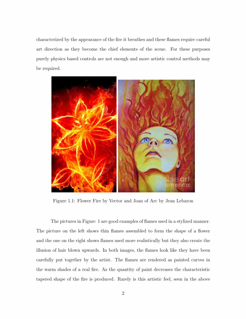
characterized by the appearance of the fire it breathes and these flames require careful

art direction as they become the chief elements of the scene. For these purposes

purely physics based controls are not enough and more artistic control methods may

be required.

Figure 1.1: Flower Fire by Vector and Joan of Arc by Jean Lebaron

The pictures in Figure 1 are good examples of flames used in a stylized manner.

The picture on the left shows thin flames assembled to form the shape of a flower

and the one on the right shows flames used more realistically but they also create the

illusion of hair blown upwards. In both images, the flames look like they have been

carefully put together by the artist. The flames are rendered as painted curves in

the warm shades of a real fire. As the quantity of paint decreases the characteristic

tapered shape of the fire is produced. Rarely is this artistic feel, seen in the above

2

images, produced in a computer simulation. In this thesis we hope to create this

artistic feel in physically based computer generated simulation.

Traditional control methods in computer simulations include wind forces, tur-

bulence or some other physics or noise based system. These models are very good at

creating realistic fire for use in visual effects. However, these control methods require

multiple iterations by the effects artist to get the desired result. It is difficult to use

these methods for artistic purposes and to control individual flames. They generally

involve the artist tweaking a number of physics based parameters which makes them

unintuitive to use easily.

In a physical fire model the shape of the flame is controlled by convection

currents generated by the heat which is in turn generated by the combustion reaction.

Therefore we focus on a system to control these convection currents and subsequently

control the shape of the flames. The inputs are reduced to a set of curves that the

artist can draw and import into the system. These curves can easily be animated by

changing the positions of the control vertices. This results in a very intuitive system

where the vision of the artist is precisely recreated. The idea of a flame as a paint

stroke is incorporated into the control mechanism to shape the flame by varying the

amount of fuel in different parts of the flame.

This thesis presents the concepts, and describes the systems developed for fluid

simulation in general and fire simulation specifically and how to create the control

curves and incorporate them into the system. The system was implemented in C++

and the curves were created in Autodesk Maya.

3

Chapter 2

Background

A flame is the visible, light emitting, gaseous part of a fire. Fire is the result

of combustion, which is an exothermic reaction between a fuel and oxidant producing

carbon dioxide, water and energy.

Figure 2.1: A Simple Flame Model, from Melek et al. [9]

As shown in Figure 2.1 fuel, preheated by ignition, when mixed with an oxi-

dizing gas starts the process, creating a reaction zone at the boundary of the flame

(flame front). The heated fuel at the center of the flame is broken down into smaller

4

molecules and radicals due to the lack of oxygen. This is very luminous and gives

flames their distinctive yellow color. As the reaction zone is approached the increasing

amount of oxidizing gas allows the chemical combustion reaction to occur. Combus-

tion continues until the stoichiometric contour (flame front) is passed and the reaction

is completed. The heat produced creates convection currents which control the shape

of the flame [9].

Flame propagation is explained by two theories: heat conduction and diffu-

sion. In heat conduction, heat flows from the flame front to the inner cone, the area

containing the unburned mixture of fuel and air. When the unburned mixture is

heated to its ignition temperature, it combusts in the flame front, and heat from that

reaction again flows to the inner cone, thus creating a cycle of self-propagation. In

diffusion, a similar cycle begins when reactive molecules produced in the flame front

diffuse into the inner cone and ignite the mixture [1].

Diffusion or Laminar flames are created when pure fuel gas from the fuel

source mixes with the oxidizing gas through the mixture zone. If the fuel is mixed

with oxidizing gas before ignition, a premixed flame is produced. This thesis focus

on diffusion flames.

In the most common type of flame, hydrocarbon flames, the most important

factor determining color is oxygen supply and the extent of fuel-oxygen pre-mixing,

which determines the rate of combustion and thus the temperature and reaction paths,

thereby producing different color hues.

Figure 2.2 shows four bunsen burner flames created by varying the mixture of

fuel and oxygen. On the left a rich fuel with no premixed oxygen produces a yellow

sooty diffusion flame, on the right a lean fully oxygen premixed flame produces no

soot and the flame color is produced by molecular radicals [2].

5

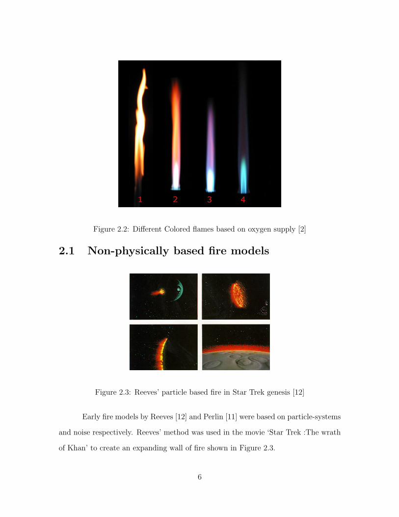
Figure 2.2: Different Colored flames based on oxygen supply [2]

2.1 Non-physically based fire models

Figure 2.3: Reeves’ particle based fire in Star Trek genesis [12]

Early fire models by Reeves [12] and Perlin [11] were based on particle-systems

and noise respectively. Reeves’ method was used in the movie ‘Star Trek :The wrath

of Khan’ to create an expanding wall of fire shown in Figure 2.3.

6

However, a large number of particles are required to hide the pointilistic nature

of the technique and the fire has a lot of grainyness. Figure 2.4 shows Perlin’s noise

based system where an animated noise texture is applied to an object. This technique

could be used to create lava like effects but isnt very useful to create fire.

Figure 2.4: Fire created with perlin noise

The approach used by Beaudin et al. [4] introduced a set of techniques used

together to produce realistic looking animations of burning objects. They use flames

as primitives instead of particles to model the fire. As shown in Figure 2.5 they

are essentially deformable chains or skeletons of vertices rooted on the surface of the

object (the sphere).

Figure 2.5: Flame Skeletons on burning spheres,from Beaudoin et al. [4]

Flame genesis and animation consist in placing flames on a surface and de-

7

forming them according to a space and time-dependent vector field in order to capture

the visual dynamics of fire. Figure 2.6 shows implicit surfaces generated around these

chains and displayed using a volumetric technique.

Figure 2.6: Flame Skeleton Rendered, from Beaudoin et al. [4]

The concept of flame skeletons helps in microscopic control of the flames but

the calculation of the vector field to modify particles is difficult for artistically driven

flames. The implicit surfaces required for visualization are complex and difficult to

generate for artistic cases.

Lamorlette and Foster [6] describe a non-physics based fire model with focus

on controlling the fire using parametric space curves. These curves evolve over time

according to a combination of physics-based, procedural and hand-defined wind fields.

A cylindrical profile is used to build an implicit surface representing the oxidation

region and particles are sampled close to this region using a volumetric falloff function.

Two levels of noise are added to provide turbulent detail. This system can be used

for animating a variety of natural fire effects and provides complete control over the

large-scale behavior.

The non-physical models described above use some kind of noise to add turbu-

lent detail which occurs as a result of the combustion reaction. These noise functions

are a drawback in microscopic control desired in highly stylized fire. In this thesis we

use a spline based control system similar to the one described by Lamorlette and Fos-

ter. However we use these control curves to control convection currents in a physical

8

simulation to achieve the highest level of microscopic control.

2.2 Physically Based Fire Simulation

A fire consists of fluids such as a fuel gas, an oxidizing gas and heat whose

behavior is described mathematically by the Navier-Stokes equation. Thus, a solver

for this equation is an integral part of a physically based fire simulator.

Fluid simulation methods are of two types, Eulerian, which discretize space by

observing the fluid through gridded data and Lagrangian which discretize the fluid

itself into smaller pieces each with its own set of parameters. A pure Lagrangian

method like Smoothed Particle Hydrodynamics [10] is useful for modeling chaotic

behavior like splashes,etc but produces discontinuity in the fluid which we do not

desire. In this thesis we use a Semi-Lagrangian Stable Fluid solver as described by

Jos Stam [13].

2.2.1 Stable Fluids

In compact form, the incompressible Navier-Stokes equations governing fluid

flow are

∂u

∂t= f − (u · ∇)u− 1

ρ∇p + ν∇2u, (2.1)

∇ · u = 0. (2.2)

Equation 2.1 represents the conservation of momentum in the fluid and equation

2.2 represents conservation of mass or divergence free flow. In the equations u is

the velocity field, p is a pressure field, ν is the kinematic viscosity of the fluid, ρ is

the density and f is an external force field. The second term of equation 2.1 is the

9

nonlinear part of the Navier-Stokes equation, it is the advection of the velocity field

on itself. The third term accounts for the pressure induced motion and the fourth

accounts for the viscous forces.

According to Melek and Keyser [9] when the speed of the flow is below the

speed of sound, the compression effects are negligible. Compressible flow equations

introduce a very strict time step restriction associated with the acoustic waves. To

avoid this strict restriction incompressible flow equations are preferred whenever pos-

sible.

The solution of the equations involves three main steps:

• Advection : This step forces a gridded quantity(velocity,density,fuel or heat) to

follow a given velocity field. This is where the idea of a semi-lagrangian approach

comes in. The key idea behind this new technique is that moving quantities

would be easy to solve if the quantity were modeled as a set of particles. In this

case the particles have to be traced back through the velocity field. As shown

in Figure 2.7 , the new velocity at x is the velocity that the particle had at a

time ∆t ago at the old location p(x,−∆t).

• Diffusion : The second step accounts for possible diffusion at a rate ν, when

ν > 0 the density will spread across the grid cells.

In the Figure 2.8 , the density of the cell (i, j) in the middle decreases by losing

to the neighbours, but will also increase due to density flowing in from the

neighbours. This results in a net difference of

ρi−1,j + ρi+1,j + ρi,j−1 + ρi,j+1 − 4ρi,j. (2.3)

For large diffusion rates, the density values start to oscillate, become nega-

10

Figure 2.7: Semi-Lagrangian Advection from Stam [13]

tive and finally diverge, making the simulation useless. Stam presents a stable

method for the diffusion step. The basic idea behind his method is to find

the densities which when diffused backward in time yield the starting densities.

Therefore, the density at cell (i, j) is

ρ(n)i,j = ρ

(n+1)i,j − ν(ρ

(n+1)i−1,j + ρ

(n+1)i+1,j + ρ

(n+1)i,j−1 + ρ

(n+1)i,j+1 − 4ρ

(n+1)i,j ). (2.4)

This is one element of the system solved by the Gauss-Seidel relaxation [14]

method.

• Projection : This routine forces the velocity to be mass conserving and diver-

gence free. Visually it forces the flow to have many vortices which produce

realistic swirly flows. This is achieved by using a result from mathematics

called Hodge-Helmholtz decomposition which states that any vector field can

be represented as a divergence free vector field and the gradient of a scalar field.

In Figure 2.9 the velocity field on the left shows swirly mass conserving flows

obtained by subtracting the gradient field on the right from the original vector

field in the center.

11

Figure 2.8: Diffusion, from Stam [14]

Mathematically, this is represented as

w = u +∇q (2.5)

where w is a vector field, u has zero divergence( ∇ · u = 0 ) and q is a scalar

Figure 2.9: Divergence free vector field,Stam

12

field. Taking the divergence on both sides of Equation 2.5 we get

∇w = ∇2q. (2.6)

This is a Poisson equation for the scalar field q. The solution is used to compute

the projection,

u = w −∇q. (2.7)

The fire model described in the next section uses the above solver to compute the

velocity, fuel and heat fields at every time step of simulation. The fire model also has

additional routines to account for the combustion reaction that occurs.

2.2.2 Fire Model

Melek and Keyser [9] present a physically accurate model of fire. Heat is also

transported with the flow of the air, and affects the buoyancy forces and changes

the flow accordingly. Sufficient heat and an appropriate mixture of the air and fuel

gas creates a combustion reaction, releasing more heat into the system. This creates

convection currents which gives the flame the desired shape. We art direct this by

controlling the convection currents from the heat, which will be described in detail

subsequently. They make various assumptions and simplifications which we carry

over to our implementation as well. These are listed below:

• The fuel gas is uniform. That is, the fuel is either burned or unburned, that any

combustible byproducts behave exactly the same as the original fuel, and that

the amount of heat produced is a function of just the amount of fuel burned.

• The compression of the gases as a result of combustion is ignored. Since basically

stable flames are simulated, it is unlikely that this compression will have a

13

significant visual effect on the solution. The total amount of gas (fuel, oxidizer,

and exhaust) in a unit volume is assumed to be constant.

• Heat and temperature are treated interchangeably.

• The pressure effects of gases at different temperatures are not modeled di-

rectly. However, the most significant effects (buoyancy of hot air, spread of

heat through the fluid) are modeled.

2.2.2.1 Gas motion in the fire model

In the “Stable Fluids” model [13] a non-reactive substance such as smoke is

carried with the motion of the fluid. Melek and Keyser [9] use the same vector field

solver, and use the resulting vector field to advect and diffuse three quantities fuel

gas, smoke and heat. Smoke is not considered for this thesis. The equations for the

motion of fuel gas and heat are

∂g

∂t= −(u · ∇)g − αgg + Sg, (2.8)

∂T

∂t= −(u · ∇)T − αT T + KT∇2T. (2.9)

Where KT is a diffusion constant, αx is a dissipation rate and Sg is the fuel gas source

term. Thus, the characteristics of the motion of fuel and heat can differ significantly,

though they are carried by the motion of the same fluid system. The external force

acting on any one cell is

F = fggg

0

−1

0

+ fT (T − Tamb)

0

1

0

(2.10)

14

where fg and fT are positive constants controlling the force components based on

gravity and temperature respectively, and Tamb is the room temperature. Hot air will

thus rise, and cold air fall, creating convection currents necessary to give the correct

flame shape. The smoke and fuel gas will tend to fall, though this effect is usually

not very noticeable (i.e. fg should be fairly small) [9].

2.2.2.2 Combustion

Melek and Keyser [9] define the equation for combustion in a cell as

if T > Tthreshold :

C = r min(dA, bdg), (2.11)

∂dg

∂t= −C

b, (2.12)

∂T

∂t= T0C. (2.13)

Where dx is the density, r is the burning rate (0 < r ≤ 1), b is the stoichiometric

mixture (the amount of air required to burn one unit of fuel), Tthreshold is the lower

flammability temperature where burning can occur, and T0 is the output heat from

the reaction. The burning rate is the percentage of the gas that can be burned in a

second.The oxygen density is defined as

dA = D − dg (2.14)

where D is the total amount of gas in each cell, which is constant and dg is the

density of fuel gas in that cell. If there is no fuel then it is filled with oxygen, and vice

versa. Although air is not all oxygen, this can be easily accounted for by adjusting

the stoichiometric mixture appropriately. Conceptually, the combustion inside the

15

cell is controlled with four parameters. Tthreshold is the temperature above which

ignition occurs. b controls oxygen requirement of the combustion and can be used to

model different reactions. T0 controls the intensity of the reaction. r controls how

quickly the gas can be burned. The heat output coming from a combustion cell can

be sufficient to start a reaction in a neighboring cell. Or it might not be sufficient

and the combustion reaction cannot continue, extinguishing the flame. Using these

parameters, the shape and the stability of the flame can be controlled [9].

2.3 B-Splines

The term ”B-spline” was coined by Isaac Jacob Schoenberg and is short for

basis spline. In this thesis B-splines are used as control curves as they recreate

AutoDesk Maya’s CV Curve tool closely. A B-spline is basically a parameterized

curve which interpolates between a set of control points.

Figure 2.10: B-spline from Wolfram Mathworld [8]

In the B-spline shown in Figure 2.10,control points are represented as P0, ..., Pn

and the knot vector as T = t0, t1, ..., tm. The knot vector is a sequence of parameter

16

values that determine where and how the control points affect the curve. The knot

vector divides the parametric space in the intervals referred to as knot spans. Each

time the parameter value enters a new knot span, a new control point becomes active,

while an old control point is discarded. In Figure 2.10 when the parameter value

switches from span t3t4 to span t4t5, the control point P0 is discarded and the control

point P4 is activated in a third order curve. The order of a curve defines the number

of nearby control points that influence any given point on the curve. The degree of

the curve is defined as p = m−n−1, where m and n are the number of control points

and knots respectively.

A basis is a set of linearly independent vectors that in a linear combination

can define a coordinate system. Basis functions are defined as [8]

Ni,0(t) :=

1 ifti ≤ t < ti+1andti < ti+1

0 otherwise

, (2.15)

Ni,j(t) =t− ti

ti+j − tiNi,j−1(t) +

ti+j+1 − t

ti+j+1 − ti+1

Ni+1,j−1(t). (2.16)

where j = 1, 2, ..., p. Using the above, the B-spline is defined as

C(t) =n∑

i=0

PiNi,p(t). (2.17)

2.4 Volume Rendering

As mentioned earlier, the heated fuel at the center of a flame is broken down

into smaller molecules and radicals due to the lack of oxygen. This is luminous and

gives the characteristic yellow color to the flame. The reactions at the flame front

release energy and some of this energy may be released in the wavelength of visible

17

light based on the type of fuel and oxidizer used.

Volumetric rendering methods are most suitable for rendering flames of this

kind. We use a simplified version of the method described in the Volumetric methods

course presented at SIGGRAPH 2010 [16], also taught by Dr.Jerry Tessendorf for the

Physically Based Effects class at Clemson University during the Spring Semester of

2011.

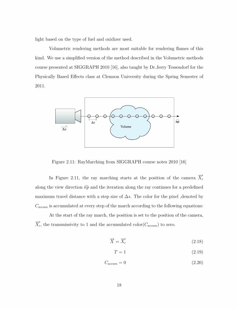
Figure 2.11: RayMarching from SIGGRAPH course notes 2010 [16]

In Figure 2.11, the ray marching starts at the position of the camera−→Xc

along the view direction n̂p and the iteration along the ray continues for a predefined

maximum travel distance with a step size of ∆s. The color for the pixel ,denoted by

Caccum is accumulated at every step of the march according to the following equations:

At the start of the ray march, the position is set to the position of the camera,

−→Xc, the transmissivity to 1 and the accumulated color(Caccum) to zero.

−→X =

−→Xc (2.18)

T = 1 (2.19)

Caccum = 0 (2.20)

18

At every step:

−−−→Xn+1 =

−→Xn + n̂p4s (2.21)

4T = e−4sρ(−→X )κ (2.22)

Cn+1accum = Cn

accum + Cd(−→X )T n(1−4T ) (2.23)

T n+1 = T n4T (2.24)

Where T is the transmissivity, ρ(−→X ) is the density at the present point of the ray

march−→X and κ is the scattering constant of the rendered quantity.

19

Chapter 3

Implementation

The simulator consists of four main components: the Fire System, the Fluid

Solver, the Curve System, and the Volume Renderer. As shown in Figure 3.1, the

Fire System is the central part of the simulator. It accepts two sets of inputs from

the user. The first is a set of physics based input parameters which includes the burn

rate, the stoichiometric ratio, the oxygen density, amount of heat produced during

combustion, the diffusion rate and the source density of fuel. These parameters

control the combustion reaction and the gas motion as described in the background

section. The second is a set of curves which the user can draw using Autodesk Maya

and then import into the program. The fire system computes the required data at

every simulation step, using the fluid solver to solve the equations for fuel gas, heat

and velocity. The resulting ignited fuel density in the grid is input to the volume

renderer which renders the image.

20

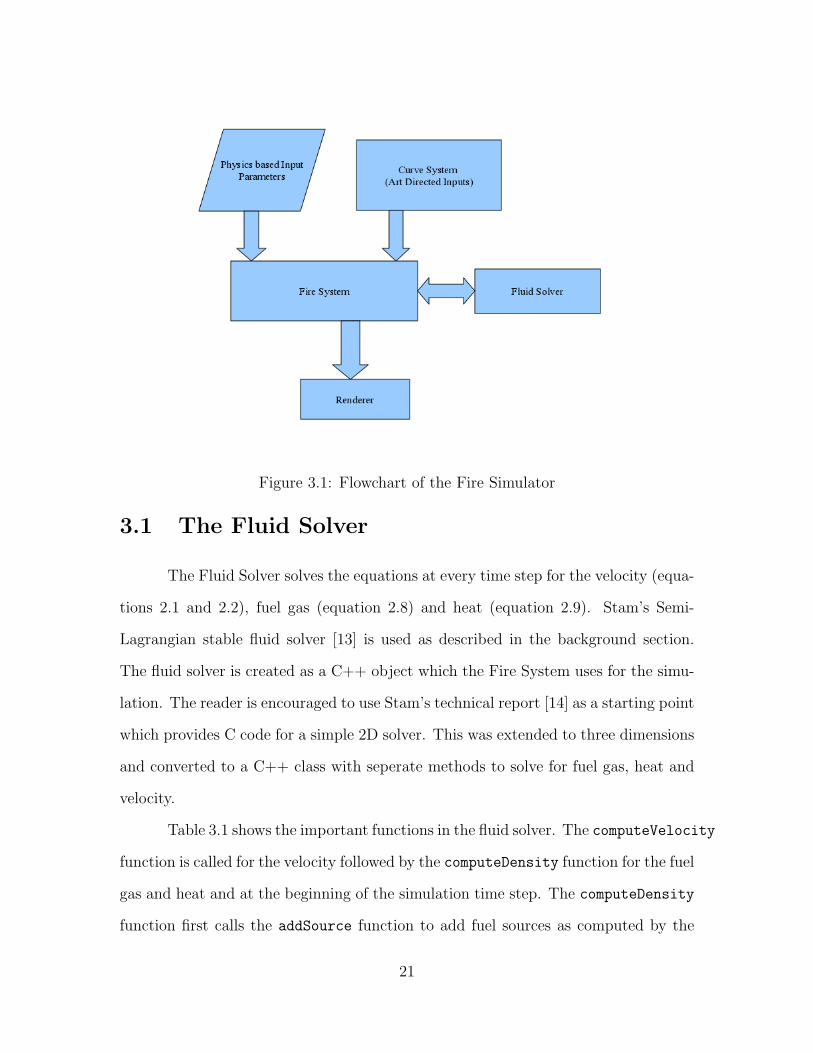
Figure 3.1: Flowchart of the Fire Simulator

3.1 The Fluid Solver

The Fluid Solver solves the equations at every time step for the velocity (equa-

tions 2.1 and 2.2), fuel gas (equation 2.8) and heat (equation 2.9). Stam’s Semi-

Lagrangian stable fluid solver [13] is used as described in the background section.

The fluid solver is created as a C++ object which the Fire System uses for the simu-

lation. The reader is encouraged to use Stam’s technical report [14] as a starting point

which provides C code for a simple 2D solver. This was extended to three dimensions

and converted to a C++ class with seperate methods to solve for fuel gas, heat and

velocity.

Table 3.1 shows the important functions in the fluid solver. The computeVelocity

function is called for the velocity followed by the computeDensity function for the fuel

gas and heat and at the beginning of the simulation time step. The computeDensity

function first calls the addSource function to add fuel sources as computed by the

21

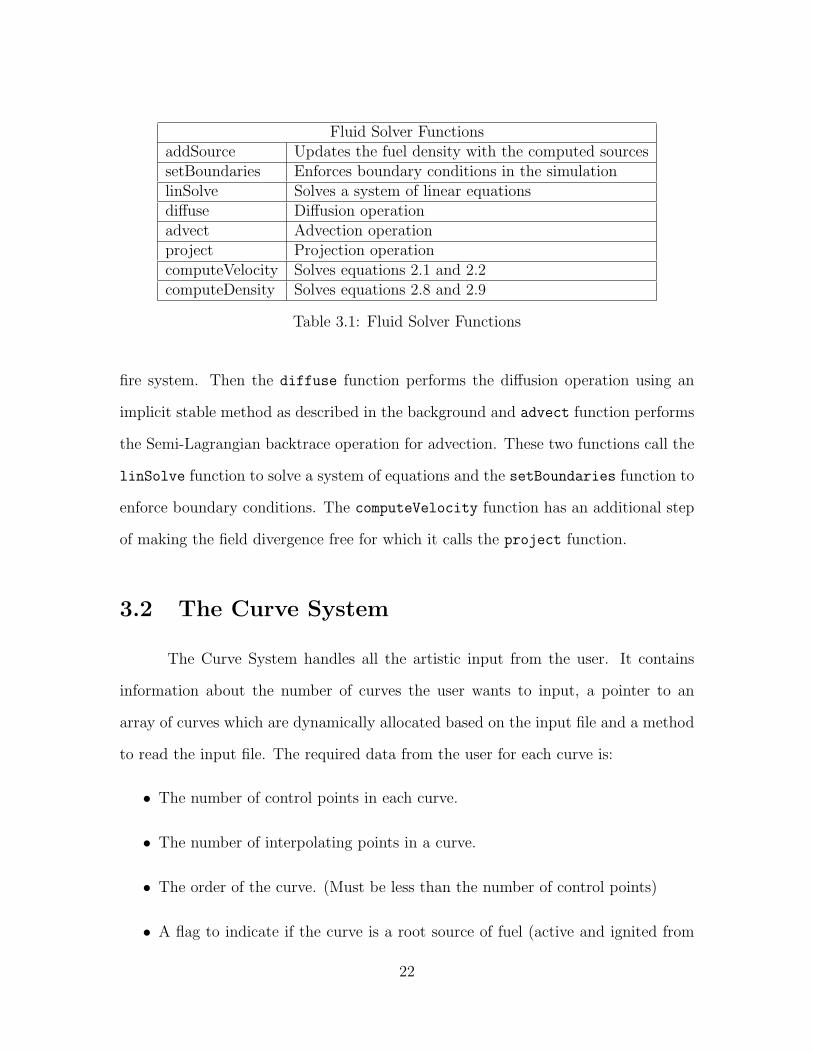
Fluid Solver FunctionsaddSource Updates the fuel density with the computed sourcessetBoundaries Enforces boundary conditions in the simulationlinSolve Solves a system of linear equationsdiffuse Diffusion operationadvect Advection operationproject Projection operationcomputeVelocity Solves equations 2.1 and 2.2computeDensity Solves equations 2.8 and 2.9

Table 3.1: Fluid Solver Functions

fire system. Then the diffuse function performs the diffusion operation using an

implicit stable method as described in the background and advect function performs

the Semi-Lagrangian backtrace operation for advection. These two functions call the

linSolve function to solve a system of equations and the setBoundaries function to

enforce boundary conditions. The computeVelocity function has an additional step

of making the field divergence free for which it calls the project function.

3.2 The Curve System

The Curve System handles all the artistic input from the user. It contains

information about the number of curves the user wants to input, a pointer to an

array of curves which are dynamically allocated based on the input file and a method

to read the input file. The required data from the user for each curve is:

• The number of control points in each curve.

• The number of interpolating points in a curve.

• The order of the curve. (Must be less than the number of control points)

• A flag to indicate if the curve is a root source of fuel (active and ignited from

22

the beginning of the simulation) or a branch source (ignites when heat from

combustion reaches it).

• A scale in the range of 0 to 1 to control the amount of fuel emitted for each

curve.

• A list of control points. (Must match the number specified before)

The fuel sources are perpetual emitters by default. Additional parameters

can be added if neccesary to control the lifetime of the flame. This can be easily

implemented as the system keeps track of time as well as the frame number.

The input to the program is a set of CV curves drawn and animated by the

user in Autodesk Maya. Maya is chosen purely for ease of animation it offers but

any other software package with curve drawing capabilities could be used. The above

data is then exported into a sequence of files by a python script which generates one

file for each frame of animation. A sample python script can be found in Appendix

A and an output file can be found in Appendix B for the reader’s reference.

The curves are all implemented as B-splines. They proved the most suitable

choice for matching the curves drawn in Maya after interpolation. C code for B-splines

from a free open source library [15] was used for curve interpolation. Additions were

made to include the flag for the fuel source, the scale factor for fuel in each curve and

to read the file input data at every frame.

3.3 The Fire System

The fire system is the central part of the program which is connected to all

the other components. It houses data structures for the coarse grids containing the

simulated quantities of velocity, fuel and heat and the directions of buoyancy and

23

gravity at each cell. It contains methods to start simulation, calculate forces , sample

and query fuel and velocity at any point in the grid and control combustion.

Fire System User Input ParametersName Description ValuenumDivisions Number of voxels along each grid side 80sideLength Length of grid side 14timeStep Length of a simulation time step 0.04diffusionRate Rate of diffusion of heat 0.01threshTemp Threshold temperature for combustion 0.0fg Scaling factor for gravity force 0.1fT Scaling factor for buoyancy force 0.2burnRate Amount of fuel exhausted by 1 unit of oxygen 1.0stoiMix Quantity of oxygen in 1 unit of air 1.0

Table 3.2: Fire System User Input Parameters

The fire system has physics based parameters to control the oxygen density,

stoichiometric ratio of air, the rate of oxidation and the amount of heat released

during combustion. Table 3.2 presents a list of all the data contained in the fire

system.

According to equation 2.10, only two constants are required to control the

forces due to gravity and buoyancy in any cell of the system. The main idea in this

thesis is to use curves to control the direction of the gravity and buoyancy vector at

each cell.

The control curve is drawn at the desired position as shown on the left side in

Figure 3.2 and the tangents to the curve are sampled at points at regular intervals

along the curve. These tangents are used as directions for gravity and buoyancy in the

system. They are injected into the force direction grid using the algorithm discussed

below.

A volumetric splatting algorithm [7] is used to inject force direction and fuel

24

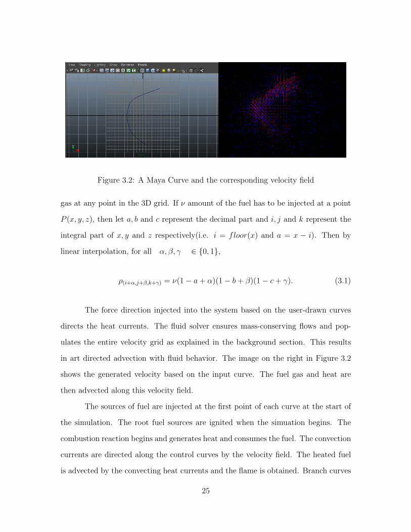
Figure 3.2: A Maya Curve and the corresponding velocity field

gas at any point in the 3D grid. If ν amount of the fuel has to be injected at a point

P (x, y, z), then let a, b and c represent the decimal part and i, j and k represent the

integral part of x, y and z respectively(i.e. i = floor(x) and a = x − i). Then by

linear interpolation, for all α, β, γ ∈ {0, 1},

ρ(i+α,j+β,k+γ) = ν(1− a + α)(1− b + β)(1− c + γ). (3.1)

The force direction injected into the system based on the user-drawn curves

directs the heat currents. The fluid solver ensures mass-conserving flows and pop-

ulates the entire velocity grid as explained in the background section. This results

in art directed advection with fluid behavior. The image on the right in Figure 3.2

shows the generated velocity based on the input curve. The fuel gas and heat are

then advected along this velocity field.

The sources of fuel are injected at the first point of each curve at the start of

the simulation. The root fuel sources are ignited when the simuation begins. The

combustion reaction begins and generates heat and consumes the fuel. The convection

currents are directed along the control curves by the velocity field. The heated fuel

is advected by the convecting heat currents and the flame is obtained. Branch curves

25

are ignited only when sufficient heat from one of the root sources reaches the first

control point.

However, due to the numerical dissipation in the fluid solver, and diffusion

of heat in the grid, the flames start fading and the sharpness is lost when they are

advected away from the sources. This behavior, although numerically correct, is a

problem for creating stylized flames. This is fixed by injecting a small amount of

fuel along the curve at each one of its interpolating points, when the advected heat

reaches that point. The quantity of fuel injected at a curve point is proportional to its

distance from the first point of the curve. Mathematically, if N represents the number

of interpolating points (the resolution) of the B-spline, (i1, ..., in) and if 0 < α ≤ 1 is

a scale factor, then the injected density at a point is

ρi =N − αi

N − 1ρ0 (3.2)

where ρ0 is the fuel gas density at the first control point of the curve. α can be

regulated to control the tapering of the flame and its length along the control curve.

This miniscule amount of fuel ignites when the heat is sufficient and the additional

convection currents generated stabilizes the shape of the art directed flame.

3.4 Volume Renderer

Once the new fuel gas and heat information are computed, the fire system

passes a pointer to the fuel gas data structure, to the volume renderer. The camera

class contains the information about the aspect ratio, field of view, position (Xc) and

orientation of the camera as well as methods to compute and return the direction of

the view vector for any pixel of the image.

26

Ideally the color of a flame depends on the mixing of oxygen with the fuel and

the temperature. The luminous heated fuel has a yellow color and the reaction zone

where the combustion happens has a reddish color. However, flame rendering is not

the focus of this thesis, so a simple approximation is used as the color of the flame.

The quantity of fuel gas density in each voxel acts as a scaling factor for a base orange

color (R=1.0, G=0.3, B=0.0 by default) which can be changed by the user. When

the fuel gas density is high the color is brighter indicating the yellow luminous part

of the flame. The consumption of fuel gas due to combustion decreases the fuel gas

density yielding a darker shade of color at the edges of the flame. This color is then

accumulated by the volume renderer to render the image.

The renderer uses the camera position and view direction to accumulate color

at every pixel by the ray-marching algorithm, as described in the background section.

The resulting color is stored in a pixmap, which is an array of sequential color values

for the whole image. This is then written into an image file using a desired file format.

27

Chapter 4

Results

In order to test the technique presented in the above sections, different cases

of stylized flames were used. The tests ran on a computer running a linux operating

system with an Intel Core 2 Quad (2.4 Ghz) processor with 4 GB of ram. The tests

were all CPU based and no GPU acceleration was used. Autodesk Maya was used

to draw and animate the control curves. No optimizations like bounding boxes were

added to the renderer used.

In the first case, the image of a set of flames shaped to form a flower shown

in Figure 1.1, was recreated through art directed simulation. Nine rendered frames

from the simulation are shown in Figure 4.1. The flames grow from combustion and

form the shape of the flower, then the convection currents that build up from the

heat produced gradually distort the shape of the flower. The simulation was done on

a 80x80x80 grid and the images were rendered at a resolution of 800x800 pixels. The

simulation was in real time (approx. 0.03 seconds per frame) and the renders took

approximately 10 minutes a frame. Root curves were used at the tips of the petals

and the stem. Branch curves are used for the leaves.

In the second case, three control curves version animated in Maya to create

28

Figure 4.1: Fire Flower rendering result

a stylized version of fire. Figure 4.2 shows nine frames out of one hundred of the

curves being animated and the corresponding renders for the animated Maya curves.

Clearly, they follow the Maya animation while exhibiting the fluid motion of fire. The

simulation was done on a 40x40x40 grid and the images were rendered at a resolution

of 500x500 pixels. The simulation was in real time (approx. 0.01 seconds per frame)

and the renders took approximately 5 minutes a frame. All three curves are root

curves.

Figure 4.3 shows a rendered image of flames directed on a set of input curves

representing a phoenix bird. Twenty-one control curves were used to create it. The

simulation was done on a 120x120x120 grid and the images were rendered at a res-

olution of 800x800 pixels. The simulation took approximately 2 seconds per frame

and the render took approximately 10 minutes.

29

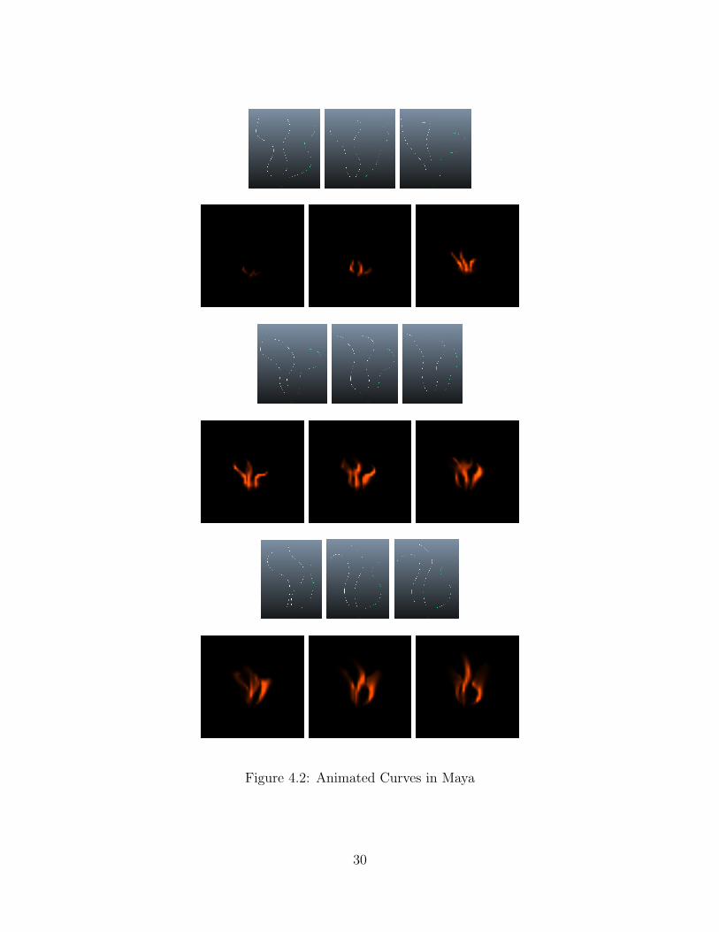
Figure 4.2: Animated Curves in Maya

30

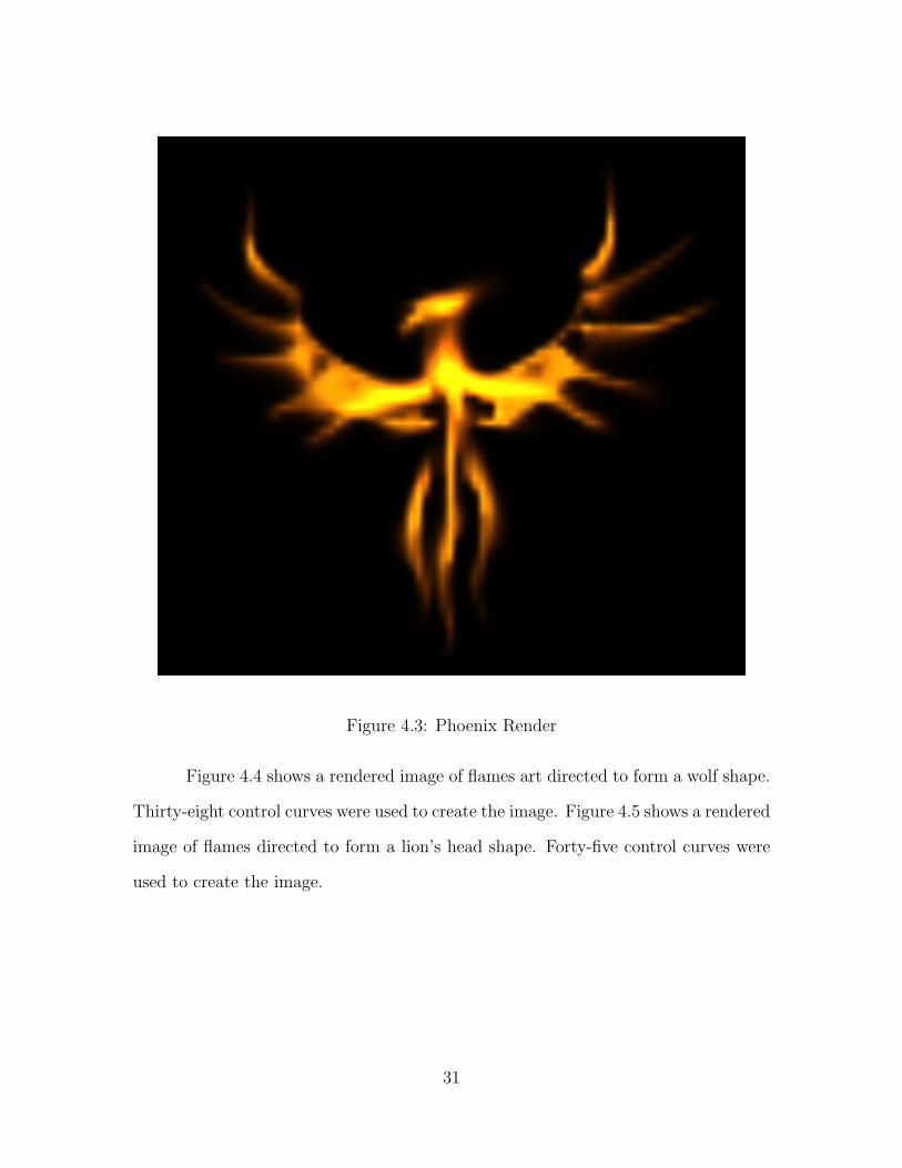
Figure 4.3: Phoenix Render

Figure 4.4 shows a rendered image of flames art directed to form a wolf shape.

Thirty-eight control curves were used to create the image. Figure 4.5 shows a rendered

image of flames directed to form a lion’s head shape. Forty-five control curves were

used to create the image.

31

Figure 4.4: Wolf Render

32

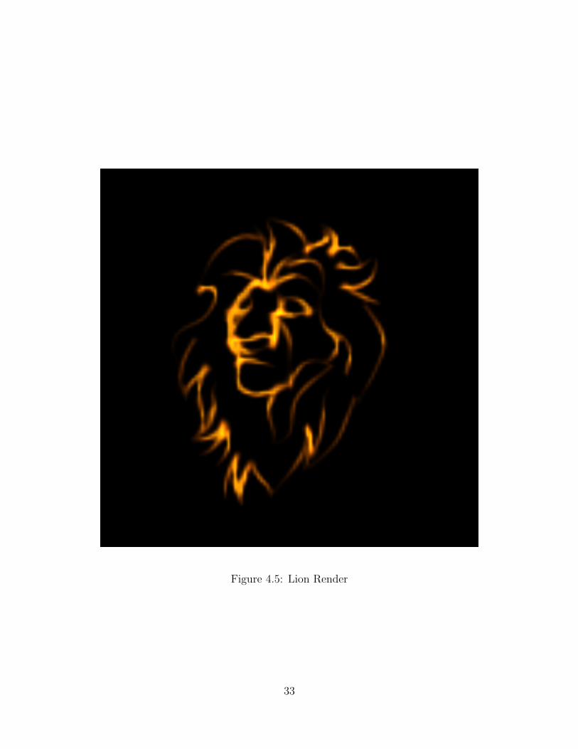
Figure 4.5: Lion Render

33

Chapter 5

Conclusion

This thesis has presented a technique to enable art direction of physically

based fire simulation. This frees the artists from using non-intuitive physical control

methods like wind fields, noise and turbulence. Traditional methods require a lot of

time-consuming iterations by the artists, with a lot of parameter tweaking, to match

the concept art. Using the technique presented, they can draw and animate control

curves in a familiar software package and then export them into the simulator. The

simulator, which uses a stable fluid solver [13] runs fast at relatively low resolutions(≤

100 voxels per side) to enable real time visualization using OpenGL. Thus, the artists

can make sure that the behavior and movement is correct before beginning the render.

The technique was applied to create single frame renders as well as animations

for highly stylized flames, which are very difficult to produce using traditional physics

based control methods. The results show that the simulated flames precisely follow

the art direction and the renders retain the artistic feel.

The thesis has described the processes involved in fluid simulation in general

and fire simulation in particular and is a good source of information for any beginner

in the field trying to build his or her own software.

34

There are a lot of possible extensions and improvements that could be added

to the model. The volume renderer could be replaced by a physically accurate ren-

derer which considers fuel-oxygen ratio, temperature and the combustion reaction at

the flame front for color computation. Stam’s stable fluid solver [13] has a lot of nu-

merical dissipation could be replaced with a more recent solver which uses advection

methods like the BFECC [5] or the Modified MacCormack [3]. The technique could

be converted into a plugin for software like Autodesk Maya or SideFX Houdini to

make use of the powerful fluid solvers and renderers that are included in them.

35

Appendices

36

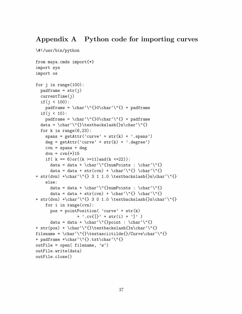
Appendix A Python code for importing curves

\#!/usr/bin/python

from maya.cmds import{*}

import sys

import os

for j in range(100):

padframe = str(j)

currentTime(j)

if(j < 100):

padframe = \char‘\"{}0\char‘\"{} + padframe

if(j < 10):

padframe = \char‘\"{}0\char‘\"{} + padframe

data = \char‘\"{}\textbackslash{}n\char‘\"{}

for k in range(6,23):

spans = getAttr(’curve’ + str(k) + ’.spans’)

deg = getAttr(’curve’ + str(k) + ’.degree’)

cvn = spans + deg

dvn = cvn{*}15

if( k == 6)or((k >=11)and(k <=22)):

data = data + \char‘\"{}numPoints : \char‘\"{}

data = data + str(cvn) + \char‘\"{} \char‘\"{}

+ str(dvn) +\char‘\"{} 3 1 1.0 \textbackslash{}n\char‘\"{}

else:

data = data + \char‘\"{}numPoints : \char‘\"{}

data = data + str(cvn) + \char‘\"{} \char‘\"{}

+ str(dvn) +\char‘\"{} 3 0 1.0 \textbackslash{}n\char‘\"{}

for i in range(cvn):

pos = pointPosition( ’curve’ + str(k)

+ ’.cv{[}’ + str(i) + ’]’ )

data = data + \char‘\"{}point : \char‘\"{}

+ str(pos) + \char‘\"{}\textbackslash{}n\char‘\"{}

filename = \char‘\"{}\textasciitilde{}/Curve\char‘\"{}

+ padframe +\char‘\"{}.txt\char‘\"{}

outFile = open( filename, ’w’)

outFile.write(data)

outFile.close()

37

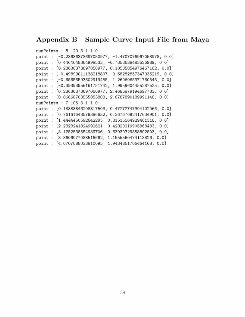
Appendix B Sample Curve Input File from Maya

numPoints : 8 120 3 1 1.0

point : [-0.23636373697050977, -1.4707076967053978, 0.0]

point : [0.4464648364998533, -0.7353538483526989, 0.0]

point : [0.23636373697050977, 0.10505054976467162, 0.0]

point : [-0.49899011138218807, 0.68282857347036219, 0.0]

point : [-0.65656593602919455, 1.2606065971760545, 0.0]

point : [-0.39393956161751742, 1.9959604455287525, 0.0]

point : [0.23636373697050977, 2.4686879194697733, 0.0]

point : [0.86666703555853808, 2.6787890189991148, 0.0]

numPoints : 7 105 3 1 1.0

point : [0.18383846208817503, 0.47272747394102066, 0.0]

point : [0.76161648579386632, 0.36767692417634901, 0.0]

point : [1.4444450592642295, 0.31515164929401318, 0.0]

point : [2.2323241824992621, 0.42020219905868483, 0.0]

point : [3.1252538554989706, 0.63030329858802803, 0.0]

point : [3.8606077038516662, 1.1555560474113826, 0.0]

point : [4.0707088033810095, 1.9434351706464168, 0.0]

38

Bibliography

[1] http://www.britannica.com/EBchecked/topic/209358/flame.

[2] http://en.wikipedia.org/wiki/Flame.

[3] S. Akwaboa. A modified maccormack’s explicit time marching scheme for solvingthe conservation equations. In Proceedings of American Physical Society, 58thAnnual Meeting of the Division of Fluid Dynamics, 2005.

[4] P. Beaudin, S. Parquet, and P. Poulin. Realistic and controllable fire simulation.In Proceedings of Graphics Interface 2001, pages 159–166, 2001.

[5] B. Kim, Y. Liu, I. Llamas, and J. Rossignac. Flowfixer: Using bfecc for fluidsimulation. In Proceedings of Eurographics Workshop on Natural Phenomena,2005.

[6] A. Lamorlette and N. Foster. Structural modeling of natural flames. In Proceed-ings of SIGGRAPH 02. ACM, 2002.

[7] D. Laur and P. Hanrahan. Hierarchical splatting: a progressive refinement algo-rithm for volume rendering. In Proceedings of SIGGRAPH 1991. ACM, 1991.

[8] Wolfram Mathworld. B-splines. http://mathworld.wolfram.com/B-Spline.html.

[9] Z. Melek and J. Keyser. Interactive simulation of fire. Technical report, July2002.

[10] M. Muller, D. Charypar, and M. Gross. Particle-based fluid simulation for in-teractive applications. In Proceedings of Eurographics/SIGGRAPH Symposiumon Computer Animation (2003). ACM, 2003.

[11] K. Perlin. An image synthesizer. In Computer Graphics (Proceedings of SIG-GRAPH 85), pages 287–296. ACM, 1985.

[12] W. Reeves. Particle systems - a technique for modeling a class of fuzzy objects.ACM Transactions on Graphics, 2(2), 1983.

39

[13] J. Stam. Stable fluids. In Proceedings of SIGGRAPH 99, Computer GraphicsProceedings, Annual Conference series, pages 121–128. ACM, 1999.

[14] J. Stam. Real time fluid dynamics for games. In Proceedings of GDC, 2003.

[15] Geometric Tools. www.geometrictools.com.

[16] M. Wrenninge, N. Bin Zafar, J. Clifford, G. Graham, D. Penney, J. Kontkanen, J.Tessendorf, and A. Clinton. Volumetric methods in visual effects. In Proceedingsof SIGGRAPH 2010. ACM, 2010.

40