advanced imaging tools for quantifying cardiac
TRANSCRIPT
ADVANCED IMAGING TOOLS FOR QUANTIFYING
CARDIAC MICROSTRUCTURE
by
Christopher Lee Welsh
A dissertation submitted to the faculty of The University of Utah
in partial fulfillment of the requirements for the degree of
Doctor of Philosophy
Department of Bioengineering
The University of Utah
August 2015

Copyright © Christopher Lee Welsh 2015
All Rights Reserved

The U n i v e r s i t y o f Ut ah G r a d u a t e Sc ho o l
STATEMENT OF DISSERTATION APPROVAL
The dissertation of Christopher Lee Welsh
has been approved by the following supervisory committee members:
Edward W. Hsu Chair 5/26/2015Date Approved
Edward V.R. DiBella Member 5/26/2015Date Approved
Rob S. MacLeod Member 5/26/2015Date Approved
Sarang Joshi Member 5/26/2015Date Approved
Yufeng Huang Member 5/26/2015Date Approved
and by Patrick A. Tresco Chair/Dean of
the Department/College/School o f ________________ Bioengineering
and by David B. Kieda, Dean of The Graduate School.

ABSTRACT
Diffusion tensor MRI (DT-MRI or DTI) has been proven useful for characterizing
biological tissue microstructure, with the majority of DTI studies having been performed
previously in the brain. Other studies have shown that changes in DTI parameters are
detectable in the presence of cardiac pathology, recovery, and development, and provide
insight into the microstructural mechanisms of these processes. However, the technical
challenges of implementing cardiac DTI in vivo, including prohibitive scan times inherent
to DTI and measuring small-scale diffusion in the beating heart, have limited its
widespread usage. This research aims to address these technical challenges by: (1)
formulating a model-based reconstruction algorithm to accurately estimate DTI
parameters directly from fewer MRI measurements and (2) designing novel diffusion
encoding MRI pulse sequences that compensate for the higher-order motion of the
beating heart. The model-based reconstruction method was tested on undersampled DTI
data and its performance was compared against other state-of-the-art reconstruction
algorithms. Model-based reconstruction was shown to produce DTI parameter maps with
less blurring and noise and to estimate global DTI parameters more accurately than
alternative methods. Through numerical simulations and experimental demonstrations in
live rats, higher-order motion compensated diffusion-encoding was shown to successfully
eliminate signal loss due to motion, which in turn produced data of sufficient quality to
accurately estimate DTI parameters, such as fiber helix angle. Ultimately, the model-

based reconstruction and higher-order motion compensation methods were combined to
characterize changes in the cardiac microstructure in a rat model with inducible arterial
hypertension in order to demonstrate the ability of cardiac DTI to detect pathological
changes in living myocardium.
iv

To my rock, Amy, and our daughter, Ruby.
In memory of my friend, Owen Stedham.

TABLE OF CONTENTS
ABSTRACT............................................................................................................................ iii
LIST OF TABLES............................................................................................................... viii
LIST OF FIGURES................................................................................................................ ix
ACKNOWLEDGEMENTS..................................................................................................xii
CHAPTERS
1. INTRODUCTION........................................... .................................................................1
2. BACKGROUND............................................. .........................................................5
2.1 Cardiac Microstructure and Function..... .........................................................52.2 Diffusion Tensor Imaging........................ .........................................................72.3 Cardiac Diffusion Tensor Imaging......... .......................................................152.4 Practical Considerations of Cardiac DTI. .......................................................262.5 Accelerating DTI Acquisition.................. .......................................................382.6 Conclusion................................................ .......................................................412.7 References................................................. .......................................................43
3. MODEL-BASED RECONSTRUCTION OF UNDERSAMPLED DIFFUSIONTENSOR K-SPACE DATA.......................... .......................................................54
3.1 Abstract..................................................... .......................................................543.2 Introduction............................................... .......................................................553.3 Theory........................................................ .......................................................593.4 Methods.................................................... .......................................................613.5 Results........................................................ .......................................................683.6 Discussion................................................. .......................................................753.7 Conclusion................................................ .......................................................783.8 Appendix................................................... .......................................................793.9 Funding Sources ...................................... .......................................................823.10 Conflicts of Interest............................... .......................................................82

3.11 Statement of Human Studies.........................................................................833.12 Statement of Animal Studies.........................................................................833.13 References....................................................................................................... 84
4. HIGHER-ORDER MOTION-COMPENSATION FOR IN VIVO CARDIAC DIFFUSION TENSOR IMAGING IN RATS......................................................88
4.1 Abstract............................................................................................................. 884.2 Introducti on....................................................................................................... 894.3 Theory............................................................................................................... 924.4 Methods............................................................................................................ 974.5 Results............................................................................................................. 1054.6 Discussion....................................................................................................... 1134.7 Funding Sources ........................................................................................... 1194.8 Conflicts of Interest....................................................................................... 1194.9 Statement of Human Studies.........................................................................1194.10 Statement of Animal Studies...................................................................... 1194.11 References.....................................................................................................120
5. EVALUATION OF MYOCARDIAL RESTRUCTURING IN RATS WITH INDUCED ARTERIAL HYPERTENSION......................................................125
5.1 Introduction.....................................................................................................1255.2 Methods.......................................................................................................... 1285.3 Results............................................................................................................. 1355.4 Discussion.......................................................................................................1485.5 Conclusion......................................................................................................1535.6 Funding Sources............................................................................................ 1535.7 Conflicts of Interest....................................................................................... 1535.8 Statement of Human Studies.........................................................................1545.9 Statement of Animal Studies.........................................................................1545.10 References.....................................................................................................155
6. CONCLUDING REMARKS...............................................................................161
6.1 Summary......................................................................................................... 1616.2 Future Directions........................................................................................... 1636.3 Final Thoughts................................................................................................1676.4 References....................................................................................................... 168
vii

LIST OF TABLES
3.1. Performance of DTI acceleration schemes in terms of fiber orientation,FA, and MD errors for an acceleration factor R = 2 .............................................. 71
3.2. Performance of DTI acceleration schemes in terms of fiber orientation,FA, and MD errors for an acceleration factor R = 4 .............................................. 72
4.1 Mean error in the presence of intravoxel phase dispersion..................................106
4.2 Mean error in the presence of shot-to-shot phase variation................................ 108
4.3 Mean error in the presence of shot-to-shot phase variation................................ 110

LIST OF FIGURES
2.1 A pair of gradient pulses used to sensitize MRI to diffusion....................................9
2.2 Sample diffusion-weighted images of an ex vivo heart...........................................11
2.3 Diffusion ellipsoid......................................................................................................14
2.4 Varying fractional anisotropy and mean diffusivity................................................ 16
2.5 Diffusion tensor parameter maps from an ex vivo heart..........................................17
2.6 DTI parameters maps..................................................................................................17
2.7 Diffusion-weighted GRE and SE pulse sequences.................................................. 27
2.8 Spin-echo, echo-planar imaging (EPI) pulse sequence...........................................28
2.9 Stimulated-echo acquisition mode (STEAM) pulse sequence............................... 36
2.10FA and helix angle maps from accelerated DTI data.............................................. 39
3.1 Sample diffusion-weighted images of specimen used in the study........................62
3.2 Sampling masks.......................................................................................................... 64
3.3 Flowchart of the model-based reconstruction algorithm.........................................65
3.4 FA-weighted fiber orientation maps..........................................................................69
3.5 Mean diffusivity maps................................................................................................69
3.6 Distribution of FA, MD, and primary eigenvector deviation..................................70

3.7 Results of pairwise, post hoc analysis of the five DTI acceleration schemesfrom Tables 3.1 and 3 .2 ............................................................................................. 73
3.8 Scan time efficiency of model-based reconstruction............................................... 74
4.1. Spin-echo diffusion encoding schemes for higher-order motion compensation .... 95
4.2 Creation of the 3D numerical motion phantom........................................................99
4.3 Effectiveness of intravoxel phase dispersion compensation at systole and diastole.......................................................................................................................105
4.4 Effectiveness of motion compensation at systole and diastole............................. 107
4.5 Effectiveness of motion compensation and cardiac cycle consistency.................109
4.6 Diffusion-weighted images of the heart obtained on a live rat with various degrees of motion compensation.............................................................................111
4.7 DTI images obtained on a live rat using velocity-, acceleration-, and jerk- compensated diffusion encoding in the same cardiac short-axis slice..................112
4.8 Unsmoothed DTI images obtained in four live rats............................................... 114
4.9 Diagram of acceleration-compensated diffusion encoding with constant amplitude gradients...................................................................................................116
4.10 Diagram of acceleration-compensated diffusion encoding incorporatedin a STEAM preparation.......................................................................................... 117
5.1. Short-axis cardiac morphology................................................................................136
5.2 Measurements of cardiac morphology.................................................................... 137
5.3 Analysis of cardiac function.................................................................................... 138
5.4 End-systole fractional anisotropy............................................................................139
5.5 End-systole mean diffusivity...................................................................................140
5.6 End-systole fiber helix angle...................................................................................141
5.7 End-systole sheet angle............................................................................................ 143
5.8 Reduced scan time fractional anisotropy................................................................ 144
x

5.9 Reduced scan time mean diffusivity....................................................................... 145
5.10 Reduced scan time fiber helix angle..................................................................... 146
5.11 Reduced scan time sheet angle...............................................................................147
5.12 End-systole and end-diastole sheet angle..............................................................150
xi

ACKNOWLEDGEMENTS
I would not be where I am today without the support of a wide range of people. I
am deeply grateful to all those that have supported me throughout the years.
During the past six years, my co-advisors, Dr. Edward Hsu and Dr. Edward
DiBella, have provided me with invaluable knowledge, skills, and lessons that would not
have been achievable elsewhere. I am very grateful for the many hours of one-on-one
help I received from each of them.
In addition, I would like to thank my lab mates, David Gomez, Samer Merchant,
and Osama Abdullah, for their continuous support throughout my time here at the
University of Utah. Rarely was there a problem that could not be solved by talking it out
with one of them. I would also like to thank those from UCAIR who provided valuable
support in my research, including Dr. Ganesh Adluru and Srikant Iyer.
Lastly, I would like to thank my wife, Amy. Her unwavering support during the
long work hours that took my away from our family was essential for me to get where I
am today. I love you.

CHAPTER 1
INTRODUCTION
Heart diseases remain the top cause of mortality in the Western world, with
approximately 600,000 deaths in the U.S. in 2014. Proper diagnosis and treatment of
cardiac diseases are necessary for potential recovery and increased quality of life in the
affected population. Understanding the mechanisms of cardiac dysfunction is key to
providing the correct diagnosis and treatment, which are necessary for improved
prognoses for patients with heart disease.
Because functions of the heart are mediated by the myocardial microstructures,
changes to the myofiber or sheet structures often lead to alternations in mechanical and
electrical properties. Characterizing cardiac microstructure can lead to improved
detection of heart disease and quantification of the extent, or stage, of disease. In
addition, tracking microstructural changes over time can evaluate disease progression or
the effectiveness of therapy. All of these can lead to more personal and effective health
care for those with heart disease.
Cardiac disease and dysfunction are traditionally evaluated using noninvasive
techniques such as EKG, echocardiography, and imaging via radiological techniques. The
majority of medical imaging techniques are used to evaluate cardiac morphology and
global cardiac function, such as ejection fraction. These methods are beneficial for
identifying failing hearts, but ultimately do not characterize cardiac microstructure and,
therefore, do not identify the low-level mechanisms of dysfunction. Histological
examination has been the gold standard for characterizing tissue microstructure in all
types of organs, but histology is inherently destructive and invasive. Diffusion tensor
imaging (DTI) has emerged as a viable alternative for characterizing biological
microstructure in a nondestructive and noninvasive manner by measuring the random
diffusional motion of water. DTI in cardiac applications is able to characterize the
microstructural arrangement of myocyte bundles, or fibers, and laminar sheets. Cardiac
DTI has the potential to correctly detect and stage disease, and provide a means to
monitor progression of disease or therapy. However, applications of DTI in the beating
heart still face substantial technical challenges before it is ready to be used for diagnosis
and monitoring of heart diseases in a clinical setting.
This work represents key improvements towards making in vivo cardiac DTI more
feasible for quantifying changes in the cardiac microstructure due to disease or recovery.
Novel methods for executing cardiac DTI in vivo are presented along with an image
reconstruction scheme designed to accurately reconstruct diffusion tensor data from
fewer MRI measurements, allowing for shorter acquisition times. These methods were
verified in numerical simulations and demonstrated experimentally in live rat models. In
the end, the usefulness of these methods in characterizing heart disease and dysfunction
are evaluated.
Chapter 2 provides a brief background in the preliminary concepts of cardiac
microstructure and the use of DTI to characterize it. The chapter details the practical and
technical challenges presented by cardiac DTI, particularly in in vivo applications. Recent
2

studies that employ DTI to characterize microstructural changes due to pathology are also
presented. In addition, recent advances in DTI that make the technique more practical and
feasible are described.
Chapter 3 describes a strategy to reconstruct diffusion tensor maps directly from
accelerated k-space data. This is accomplished by modifying the objective function in
traditional compressed sensing to be a function of the desired diffusion tensor instead of
the magnitude of the individual diffusion-weighted images. Because the objective
function is a function of the diffusion model, the method is referred to as model-based
reconstruction. The proposed method is compared against other more common
reconstruction techniques and control cases. A quantitative comparison between the test
cases was performed to determine which method produced the most accurate DTI maps
from accelerated diffusion data.
Chapter 4 describes a methodology for implementing higher-order motion
compensation in diffusion-encoding MRI to obtain DTI measurements in the beating
heart. The study compares the performance of previously established diffusion-encoding
methods, those with no motion compensation and velocity-compensation, to the
performance of novel diffusion encodings with acceleration- and jerk-compensation via
gradient moment nulling. All methods were evaluated in a realistic numerical phantom of
the beating heart and in live rats. Acceleration-compensated diffusion encoding was
found to provide the best balance of motion artifact reduction and SNR preservation,
which was necessary to derive accurate DTI parameter maps.
A preliminary study that combines the methodologies developed in Chapters 3 and 4
is presented in Chapter 5. DTI scans were performed in transgenic rats, using
3

acceleration-compensated diffusion encoding, prior to and two weeks after induction of
arterial hypertension to observe changes in the cardiac microstructure due to increased
after load. In vivo DTI was essential to observe the changes in key DTI parameters that
would otherwise not be detectable if a terminal study was performed. Model-based
reconstruction of diffusion tensor maps was performed to show the potential of reducing
acquisition time without losing the proportional amount of accuracy.
The concluding chapter of this document, Chapter 6, provides a discussion regarding
the advantages and disadvantages of acceleration-compensated diffusion encoding for in
vivo DTI and reducing scan time with model-based reconstruction, and offers some
recommendations for improvements on the methods presented herein as well as future
areas of investigation.
4

CHAPTER 2
BACKGROUND
2.1 Cardiac Microstructure and Function
Myofiber structure of the heart is an important determinant of its function [1]. The
distribution of myofiber orientation within the heart wall is the main determinant of stress
distribution and myofiber shortening throughout the wall [2], and therefore, of cardiac
perfusion [3] and structural adaptation [4], [5]. Myofiber structure also plays a key role in
electrical propagation inside the heart [6]. Myofiber architecture is known to be altered in
some cardiac diseases, such as ischemic heart disease and ventricular hypertrophy [7].
Therefore, detailed knowledge of myocardial fiber microstructure promises to lead to
better understanding of the heart function in health and disease.
Anisotropy is one of the most consistent observations in studies of the heart. It is
present in cardiac material and functional properties at essentially all scales. This
includes, in the molecular scale, the arrangement of collagen fibers and actin-myosin
contractile structures at the subcellular level, the arrangement of myocytes with respect to
their neighbors at a cellular level, and the observable texture of the cardiac muscle at an
organ level. For this reason, fiber orientation is an intrinsic part of cardiac structure, and
affects its local material properties, mechanical and electrical behaviors, and other
functions of the heart. The ability to extract fiber structure information from an organ or

samples of tissue is vital to explain these effects. Over time, many have proposed
mathematical and theoretical models for different aspects of the heart as technological
advances make fiber structure information available. Notable examples in biomechanics
include constitutive characterization of tissues and its subsequent use in functional
modeling of the whole heart. Experimental observations like mechanical testing of
myocardial tissue have shown that mechanical properties are dependent on the tissue
microstructure such as fiber orientation, the sheet-like formation of fibers (i.e.,
lamination), and the associated arrangement of the extracellular matrix. The mechanical
properties have been described through several mathematical formulations of constitutive
behavior [8], [9]. To reach meaningful results from the application of these models,
information on organ geometry and tissue anisotropy are both necessary [10], [11].
The above structure-function relationships also apply to cardiac electrophysiology
[12], and should be reflected in simulation of electrical propagation and coupled electro
mechanical modeling. It is well established that electrical conductivities of cardiac tissues
also exhibit anisotropy [13], [14] and that those are determined by tissue microstructure,
in particular, the local orientation and lamination of cardiac fibers. In general, anisotropic
description of tissue properties is a crucial component for coupled, electro-mechanical
modeling of the heart [15], which requires the integrative modeling of electrical
activation, force development and mechanical deformation based on anisotropic tissue
properties. For example, anisotropic cardiac tissue properties have been used to produce
comprehensive models seeking to provide explanations for the basic mechanisms for
ventricular contraction, expansion, and torsion [16].
6

2.2 Diffusion Tensor Imaging
The power of MRI is derived from its sensitivity to the molecular dynamics of water,
which in turn closely follows the microstructure of tissues. By generalizing the principles
of diffusion MRI to describe anisotropic diffusion in 3D space, diffusion tensor imaging
(DTI) can be used to characterize myocardial structures. In the heart, although the exact
biophysical mechanism is incompletely understood, it has been suggested that water
diffusion anisotropy arises from the combined effects induced by the cardiomyocytic
membrane, extracellular connective tissue, and microvasculature [17].
Mathematical descriptions of the macroscopic and microscopic consequences of
molecular diffusion were originally provided by Fick and Einstein, respectively [18],
[19]. Torrey [20] then incorporated anisotropic translational diffusion in the MRI Bloch
equations as an additional source of signal attenuation. About a decade later, Stejskal and
Tanner [21] solved the Bloch-Torrey equation for the case of free anisotropic diffusion in
the principal frame of reference. The pioneering work on combining MRI and diffusion
anisotropy came from the rigorous formalism of the diffusion tensor by Basser et al. [22],
[23]. In this section, the physical basis of DTI and its experimental design strategy will be
discussed.
2.2.1 Diffusion and the MR Signal
In general, there are two types of diffusion that are of interest in MRI: movement of
molecules from regions of higher to lower concentrations, and the random or Brownian
motion of molecules due to thermal energy. For distinction, the latter is often referred to
as self-diffusion. For the sake of simplicity, from this point forward, the term “diffusion”
7

will refer to self-diffusion, particularly the self-diffusion of water.
In statistical mechanics, the average displacement along a given axis, say the x-axis,
(x), of diffusing water molecules is related to the diffusion coefficient, D, via the
Einstein’s equation
<x> = V2DA, (21)
where A is the diffusion time (e.g., time between leading edges of diffusion encoding
gradient pulses) and D is the diffusion coefficient. In biological tissue, D decreases,
compared to free water, due to obstructions imposed by microstructure (e.g., cell
membranes, fibers, etc.). These obstruction effects are generally anisotropic (i.e., not
uniform in all directions), which gives rise to a preferred direction of water diffusion
because, intuitively, water molecules will diffuse fastest in the direction parallel to tissue
fibers. DTI can be utilized in cardiac tissue in order to characterize its fiber structure,
such as fiber orientation or the organization of fibers.
In MRI, linearly varying magnetic field gradients (or simply gradients) are used to
manipulate the resonance frequencies of the individual magnetic moments, or spins, that
contribute to the detected signal. Specifically, the relative frequency, with respect to a
spin located at the origin, at which a spin located at r precesses can be expressed as
« ( r, 0 = -Y G(t) ■ r ( t) , (2 2)
where y is the gyromagnetic ratio (for 1H) and G is the applied 3D gradient field. Now,
consider the scenario in Fig. 2.1, where a spin is first subjected to a gradient pulse of +G
amplitude, followed by an equal but opposite (-G) pulse. Suppose during the first pulse,
the spin is located at rx, and as such, it would acquire a phase of
44 = —Y G • 5, (2 3)
8

9
G
V
A
5 -G
VA
>
Figure 2.1: A pair of gradient pulses used to sensitize MRI to diffusion. An individual spin is tagged with a given phase during the first gradient pulse, depending on its spatial location. The second gradient pulse undoes the phase tagging for stationary spins. For spins that move or diffuse between the pulses, the resulting phase after the second pulse is proportional to the distance moved between the two gradient pulses.
where 5 is the duration of the diffusion gradient pulses. Furthermore, suppose the spin
has moved during the time between the two gradient pulses and is located at r2 during the
second pulse, the spin would acquire an additional phase
The phase accumulated by the spin is, therefore, proportional to the distance the spin has
moved from rx to r2. If a spin has not moved, the cumulative phase will be zero.
The effect of diffusion in the presence of a sensitizing gradient on the MRI signal can
be found by solving for the expected value of the phase dispersion of an individual spin,
which is a random process, according to
= y G ■ r2 5. (2.4)
Consequently, the cumulative or net phase is
0 n e t 0 2 + 0 1= — y G ■ r2 5 + y G ■ rx 5 = -y G ■ ( r 2 - r i ) 8
(2.5)
I = Iq J e x p ( - i^ n e t ) P ( r 2 | r i)d $ , (2.6)

where I0 is the diffusion-independent signal and P( •) is the probability density function
of the diffusion, which in the case of free or unrestricted diffusion is a Gaussian
distribution with a standard deviation specified by the Eq. (2.1), a = V2DA.
It can be shown that when diffusion is encoded using a pair of rectangular pulses of
opposite polarity and with magnitudes equal to G = |G|, like those in Fig. 2.1, the
Stejskal-Tanner expression for diffusion can be derived
I = I0 ex p (-•y2G252(A — 5 /3 )D) = I0 exp(-bD ), (2 7)
where b = y2G252(A — 5/3) is the so-called diffusion-weighting factor. Therefore,
diffusion manifests itself in the acquired image as a loss or attenuation of signal. In turn,
the diffusion coefficient D, better known in MRI as the apparent diffusion coefficient
(ADC), can be computed from MRI signals acquired with and without the diffusion
encoding gradients, I and I0, respectively, according to
D = ( - 1 /b ) ln (I/I0). (28)
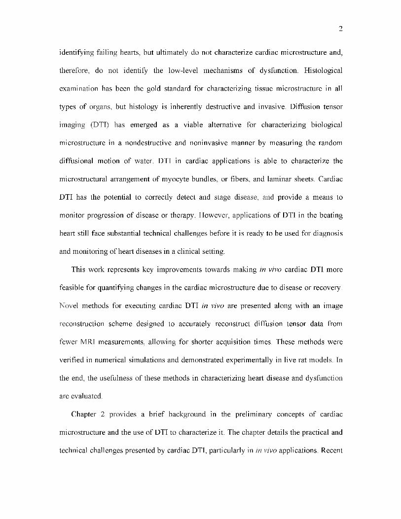
To illustrate the effect of diffusion encoding and the underlying myocardial fiber
structure, Fig. 2.2 shows a nondiffusion-weighted image, I0, along with a diffusion-
weighted image, I, of a human heart sample. Because the amount of diffusion-induced
MRI signal attenuation is dependent on the rate of diffusion along the direction of the
encoding direction, the fact that different regions of the cardiac left ventricle have
different intensities is an indication that the underlying myocardial fibers are oriented in
different directions.
10
11
Figure 2.2: Sample diffusion-weighted images of an ex vivo heart. Nondiffusion-weighted cardiac sample (top-left) shown alongside diffusion-weighted images of the same sample encoded in the x-direction (top-right), y-direction (bottom-left), and z-direction (bottom- right) with a b-value of 2000 s/mm2.
2.2.2 MRI of Anisotropic Diffusion
The orientation-dependence of the effect of anisotropic diffusion on the MRI signal
can be more easily explained by first considering a special system in which the principal
axes of diffusion coincide with the laboratory gradient axes. Specifically, suppose the
diffusivities are Dx, D2, and D3 along the principal axes, which are aligned with the
laboratory x-, y-, and z-axes, respectively. The combined signal attenuation is given by
the superposition of Eq. (2.7) applied to each axes, or
/ = /0 exp(- b xDt - byD2 - bzD3) , (2 9)
where b ; = y2G! 52(A — S/3) is the diffusion weighting factor associated with each

12
i = x, y, z axis. Moreover, provided that the diffusion encoding gradients in different axes
are identical in timing but differ only in their relative amplitudes, Eq. (2.9) reduces to
Dx 0 0 'I = I0 exp (—b u T 0 D! 0 u ), (2.10)
0 0 Dz
where u is the unit vector denoting the composite gradient direction (e.g., u = [1 0 0 T,
[0 1 0 T and [0 0 1 T for the x-, y- and z-directions, respectively). Implicit in Eq. (2.10)
I = I0 exp I - b g TRT R g = I0exp ( - b g TD g ), (2.11)
is that G = ^G! + G^ + G| should be used in Eq. (2.7) for computing the diffusion
weighting factor.
The obvious limitation of Eq. (2.10) is that, more often than not, the principal
diffusion axes do not coincide with the laboratory axes. In the general case when the
coordinate systems are not aligned, Eq. (2.10) can be modified by mapping the laboratory
axes onto the diffusion coordinate system via the transformation u = Rg, resulting in
D! 0 0 - 0 D2 0
.0 0 d3.
where g is the directional unit vector (in laboratory coordinates) of the diffusion encoding
gradient, and
"D-i 0 0 1 D xx D xy D xz(2.12)
is the rank-2 tensor that characterizes the diffusion in 3D space, otherwise known as the
diffusion tensor. Since diffusion cannot physically be negative, the principal diffusivities
(i.e., the diagonal terms of the diffusion tensor) must be non-negative, which results in
the diffusion tensor being positive semi-definite. Many diffusion tensor-fitting algorithms
incorporate the positive definiteness constraint in their fitting [24]. It can be seen from
D- 0 0 D xx yxD zxD
D = Rt 0 D2 0 R = D xy Dyy D N
. 0 0 D3. D xz D N
NNQ

13
Eqs. (2.11) and (2.12) that the major task in DTI is to use the choices of encoding
gradient directions g to selectively probe the elements of the diffusion tensor.
Following similar derivations as described above, the signal attenuation due to
anisotropic diffusion in the presence of time-varying gradient waveforms can be
alternatively expressed as [25]
where b^ (i, j belongs to x, y, z) corresponds to individual entries of the “b-matrix”, b.
2.2.3 Experimental Strategy
Regardless of whether the approach described by Eqs. (2.11) or (2.13) is used, the
typical DTI experiment consists of acquiring a series of diffusion-weighted MRI scans
encoded using one or more b-values along at least six noncollinear gradient directions,
(since the diffusion tensor is a rank-2, symmetric tensor as seen in Eq. (2.12)) and
estimation of the diffusion tensor on pixel-by-pixel basis via appropriate curve fitting of
the observed signals to the signal attenuation equation. Given that a nondiffusion-
weighted image, commonly referred to as a b0 image, is needed to estimate the diffusion-
independent signal I0 the minimum scan time for a diffusion tensor experiment is,
therefore, seven times longer than a conventional scan of the same anatomy. Directly, the
estimated diffusion tensor bears little use for inferring the tissue microstructure, since the
relevant information is embedded in the tensor elements.
Mathematically, the surface of equal probability at a given time for finding water
molecules, which are initially located at the origin but subject to anisotropic diffusion

14
governed by a diffusion tensor, is an ellipsoid. As an ellipsoid is described by the lengths
and orientations of its major and minor axes, the diffusion tensor is related to the
magnitudes and directions of the underlying principal diffusion processes by its
eigenvalues and eigenvectors. Consequently, by applying the linear algebraic eigenvalue
decomposition, the diffusion tensor can be converted into a product between a diagonal
matrix of its eigenvalues and transformation, or rotation, matrix consisting of its
eigenvectors. According to Eq. (2.12), the eigenvalues and the eigenvectors of the
diffusion tensor correspond to the diffusivities as observed along the principal axes of
diffusion and the orientations of the axes, respectively, as shown in Fig. 2.3. The central
premise of DTI is that the direction in which water diffusion is the fastest, in other words
the eigenvector of the largest diffusion tensor eigenvalue, coincides with the local tissue
fiber orientation.
To make the derived parameters even more intuitive in cardiac DTI, the fiber
Figure 2.3: Diffusion ellipsoid. The amount of diffusion in the principal axes is proportional to the eigenvalues D1, D2, and D3. The orientations of the three principal axes are determined by the eigenvectors evl, ev2, and ev3.
e\

orientations are often reported in terms of their helix angles and, to a less extent,
imbrication angles. On the other hand, the diffusion tensor eigenvalues are commonly
used to compute the mean diffusivity (MD) and fractional anisotropy (FA) index
MD = (Di + D2 + D3)/3 , (214)
15
FA =(D! - M D 2 + (d 2 - M D 2 + (d 3 - M D 2 (215)
D! + D2 + D!
To a first approximation, the MD is proportional to the size of the diffusion ellipsoid,
whereas the FA is analogous to the standard deviation of its eigenvalues or the aspect
ratio of the diffusion ellipsoid as seen in Fig. 2.4. The FA is a normalized quantity, with
FA of zero and unity respectively denoting no and infinite anisotropy.
In practice, not only are the above indices convenient quantities that capture the
overall magnitude of diffusion and the degree of anisotropy, but they also have the nice
feature of being rotationally invariant or, in other words, do not depend on the
orientations of the diffusion principal axes. The fiber orientation helix angle and the
scalar DTI MD and FA for the same specimen shown in Fig. 2.2 are illustrated in Figs.
2.5 and 2.6.
2.3 Cardiac Diffusion Tensor Imaging
DTI has been used to characterize tissue structure in a number of applications,
including studies of the myocardium and its functions. This section offers a brief survey
of these applications, which include validations of DTI (Section 2.3.1), tissue specimen
characterization (Section 2.3.2), DTI of cardiac pathophysiology (Section 2.3.3), and
examples of clinical applications of DTI (Section 2.3.4)

16
Fractional Anisotropy
© • i
Figure 2.4: Varying fractional anisotropy and mean diffusivity. Diffusion ellipsoids with varying fractional anisotropy (FA) and mean diffusivity (MD) values.
2.3.1 Validation of Myocardial DTI
As with any newly introduced imaging technique, the extent to which DTI is useful,
in the current case for characterizing myocardial structures, requires it to be validated
against the commonly accepted gold standard for the same measurements, which is
histology. Early applications of DTI in the myocardium were soon followed by studies
that directly correlated DTI-measured myocardial fiber orientations, which are
technically the local direction in which water diffusion is fastest, with histology including
separate studies performed on freshly excised canine right ventricular sample [26],
perfused [7] and formalin-fixed whole rabbit left ventricle [27]. These studies using

17
Figure 2.5: Diffusion tensor parameter maps from an ex vivo heart. Maps representing the diffusion tensor parameters derived from the diffusion data shown in Fig. 2.2. The rows and columns correspond to the 3 x 3 diffusion tensor as seen in Eq. 2.12. The images on the diagonal are scaled from 0 to 1, while the off-diagonal images are scaled from -0.25 to 0.25.
Helix Angle FA Mean Diffusivity
- 90 ° 0 ° 90 ° 0 0.25 0.5 0 0.5 1.0(x 10'3 mm2/s)
Figure 2.6: DTI parameters maps. Maps representing helix angle (left), fractional anisotropy (FA) (middle), and mean diffusivity (right) derived from the diffusion tensor data shown in Fig. 2.5.

diffusion imaging MRI have helped establish DTI as a valid alternative to histology for
measuring myocardial fiber orientation. Because the studies were performed on
differently prepared myocardial samples, they also suggest that DTI, at least for fiber
orientation mapping, is immune to the effects of tissue preparation like fixation, for
example. In the study performed on freshly excised canine ventricular sample, the fiber
orientation helix angles measured by DTI and histology were found to differ on average
by 2 - 5° [26]. The excellent correspondence between DTI and histology results supports
the hypothesis that the first eigenvector of the MR diffusion tensor coincides with the
orientation of the local myocardial fibers.
Being a noninvasive technique, DTI may be uniquely suited to help address the
controversy over the existence of myocardial laminar or sheet structure. The concern was
that the laminar structure is not an intrinsic property of the myocardium, but an artifact
introduced in the tissue preparation steps (e.g., fixation and sectioning) of histology [28],
[29]. In DTI, one would intuitively expect myocardial sheets to make water molecules
diffuse more freely within rather than across any laminar structure. Consequently, the
existence of myocardial sheets would manifest in (a) distinct second and third
eigenvalues in the myocardium, and (b) the eigenvectors associated with second and third
eigenvalues to exhibit a nonrandom organization. Indeed, distinct populations of second
and third eigenvalues within statistical confidence levels were observed in the canine
myocardium [30]. Nonrandom second eigenvector fields were reported in fixed mouse
hearts [31]. The organized appearance of the second eigenvector was also observed in ex
vivo human myocardial specimens [32]. Moreover, similar organized appearance was
also observed in fresh excised [26] and perfused unfixed myocardium [7], which suggests
18

neither tissue fixation nor sectioning as source of diffusion anisotropy observed in DTI.
The link between the DTI second eigenvector and myocardial laminar structure is
further supported by findings of a subsequent study comparing DTI and cut-face ink blots
of the bovine myocardium [33], showing a parallel relationship between the eigenvectors
and symmetry axes of the myocardial architecture. Specifically, the first, second, and
third eigenvectors corresponded to the fiber, sheet, and sheet normal directions,
respectively [33]. The use of cut-face ink blots provided a method in which fiber and
sheet orientations could be measured under the same conditions when using different
modalities (optical vs. MRI), by minimizing the possibility of tissue alterations between
data acquisitions.
2.3.2 Applications of Cardiac DTI
Since its advent, DTI has been used to characterize the normal myocardium in vitro
and ex vivo across several species. In one study on healthy goat hearts [5], the helix angle
was found to vary transmurally across the left ventricle (LV), with the steepest slope
found in the anterior and septal sites. Similar variability of the helix angle slope was also
observed in rabbit hearts [34] and mouse hearts [31]. The heterogeneity of the anisotropy
index, FA, was measured in sheep [35] and was found to vary transmurally across the
myocardium. The variability of cardiac microstructure was also studied across different
species [36], which showed significant fiber structural differences between any of the
pairs of species examined.
High resolution DTI (100 p,m) was introduced [31] in mouse hearts, which allowed
for more detailed characterization of myocardial microstructure. Cardiac studies using
19

high resolution DTI were consequently performed to illustrate microstructural changes in
the myocardium following dyssynchronous heart failure in canines [37] and myocardial
infarction in sheep [38]. Another high-resolution DTI study linking cardiac
microstructure to its function was performed in rats [39] and found that wall thickening
during contraction is related to changes in fiber and sheet structure configurations.
DTI and 3D MRI imaging created the possibility of characterizing the organization of
myocytes in 3D space, rather than in a 2D plane as is done in histology. Studies using
alternative methods to DTI suggested that not all myocardial fibers are oriented
circumferentially, but that there are intruding fibers that are oriented radially [40]. Other
studies using histology [41] and confocal microscopy [42] found evidence that the
organization of myocytes vary in 3D space. Studies using DTI on postmortem porcine
hearts found that the ventricular mass is arranged as a mesh of tangential and intruding
fibers and that there is no support for a unique myocardial band [17], [43], [44].
In another interesting study [45], a nonexchanging, two-component diffusion tensor
model was fitted to diffusion-weighted images obtained in rat hearts ex vivo. The results
suggested the existence of at least two distinct components of anisotropic diffusion,
characterized by a “fast” component and a “slow” component, which exhibited highly
similar orientations. It was suggested that the fast and slow components corresponded to
the vasculature and cellular components, respectively, of the myocardium.
2.3.3 DTI and Cardiac Pathophysiology
The presence of cardiac disease often involves multiscale myocardial structure
remodeling, which is reflected by variations of some DTI parameters. Despite the lack of
20

comprehensive understanding regarding the mechanisms governing these variations, the
correlation of DTI parameters with health and pathology have shown promise in potential
tools for diagnosis and computational modeling of disease, and its progression.
DTI studies on multiple animal models suggest sensitivity to pathology, which imply
that DTI may be clinically useful in determining the extent of disease extent or the
effectiveness of therapy. Previous studies have shown that fiber disarray, detectable by
DTI, often accompanies cardiac disease. For instance, a reduction of tissue diffusivity
was observed on isolated ischemic rabbit hearts [7]. The same observation was confirmed
in another study performed on excised hearts of infarcted porcine, which also associated
infarction with flatter helix angle [46]. The effects of infarction on the border and remote
zones have also been studied using DTI. In a study where fiber structure of excised rat
hearts was visualized in 3D [47], it was shown that infarct areas change from a normal
fiber distribution pattern to orthogonally intersecting networks similar to a mesh, which
extend across the infarcted area to the border zones. A similar study on porcine models of
infarction [48] showed that infarct border zone, delineable by DTI contains viable
myocardial strands, which may have an effect on postinfarct electrophysiology.
The effects of infarction on FA, apparent diffusion coefficient (ADC), and helix angle
have also been studied. When compared to its healthy state in pigs, the infarcted
myocardium exhibits a decrease in FA value, increased ADC, and a flatter helix angle
[49], [50]. These changes insinuate fiber disarray, which is observed accompanying
fibrosis [51]. Additional observations, as well as multiple speculative explanations for
their appearance have been made in separate studies, for example: FA has been suggested
as an indicator of functional recovery following heart transplant in canines [52].
21

Imbrication (or intrusion) angle increases were observed in hypertrophic mouse hearts
[53]. Structural changes were observed during the progression of left ventricular
myocardial infarction [54], and following surgical restoration [38]. Further, the double
helix myocardial structure shifted more leftward around the infarcted myocardium, and
the redistribution of fiber architecture correlated with the infarct size and left ventricular
function [50], [55]. Finally, myocardial architecture is linked to initiation and
maintenance of reentrant arrhythmias [6] as well as the mechanical coupling during
systolic wall thickening [26], [56].
In terms of modeling of pathophysiology, DTI data have been used, within the realm
of cardiac biomechanics, in a wide variety of studies. Some aim to improve our
understanding in the overall structure-function of the heart [57], [58]. Others seek to
measure stress, strain, and other biomechanical parameters by constructing finite element
models for myocardial infarction [59]—[61], as well as computational representations of
cardiomyopathy [62], and cardiac growth [63]. Additional researchers are also using DTI
data to characterize the effects of fiber structure remodeling in animal disease models
[54], [64], [65], and to quantify differences across species [36], or across the cardiac
cycle [66]. A number of studies proposed that ventricular fiber orientation is a result of
mechanical feedback [2], [4], [67], [68]. These studies applied biomechanical simulations
and optimization approaches to derive fiber orientations leading to, for instance, uniform
mechanical load. A study on ovine left ventricle, however, indicated difficulties to predict
fiber orientations based on mechanical feedback [69]. It was suggested that detailed
geometrical information is required for prediction of fiber orientation.
A detailed knowledge of the ventricular fiber structure is important for understanding
22

the nature of cardiac electromechanics in healthy, disease, and intermediate conditions.
During postinfarct healing, the fibers rearrange parallel to fibers outside the border zone
[70]. Also, local fiber aggregation is disturbed increasing or decreasing fiber density due
to edema, and may be affected by increased fibrosis. Tissue structure becomes irregular,
or discontinuous, which may promote electrical function anomalies or mechanical failure
[38], [70], [71]. Generally, the alteration of fiber structure in most cases is a dynamic
process that accompanies healing or remodeling, and varies over time. In a study on a
mouse model, the infarcted region measured lower ADC than the remote region, and the
low values increased with time subsequent to infarction. Increased FA peaked after 28
days, which may be associated to the observed development of structured collagen fibers
in the area [54]. At the molecular level, FA was found to be associated with decreased
induction of endothelin-1 (ET-1) and caspase-3, improved adenosine triphosphate (ATP)
storage in the myocardium, and functional recovery of the myocardium after ischemia
[52]. Another study on infarcted sheep hearts revealed a significant reorganization of the
three-dimensional aggregation of adjacent fibers in the remote zone of remodeled hearts
[72]. Regardless of angle classification, a positive (rightward) shift in myocardial helix
angle is observable in all layers of the remote zone, in particular the subepicardium.
In conjunction with strain, DTI has been used to study hypertrophic cardiomyopathy
(HCM) in humans establishing a relationship between myofiber disarray, mainly
measured by FA, and hypokinesis, measured by tissue deformation [73], where HCM
exhibited locally reduced diffusion FA, which indicate myofiber disarray. The same areas
also showed decreased myocardial strain, especially in the direction perpendicular to
fibers within the local sheet structure, which had the highest correlation between FA and
23

24
hypokinesis.
2.3.4 In Vivo Cardiac DTI
The noninvasive nature of DTI presents the opportunity that it could be used to
characterize myocardial structures in vivo in both animals and humans, which would be
desirable to better understand both healthy heart functions as well as disease progression.
Earliest works of in vivo cardiac DTI were simply to demonstrate the feasibility of the
technique, which is not trivial due to complications arising from the beating motion of the
heart, or to document its sensitivity to myocardial remodeling in diseases. Initial studies
performed on perfused rat hearts [3] and on human hearts in vivo [74], [75] showed that
not only was diffusion MRI on the beating heart technically feasible, but also fiber
architecture of the myocardium imparted anisotropy on the water diffusion. Subsequent
studies revealed that tissue strain in the beating myocardium affects the observed
diffusion signal, which can be eliminated by either retrospective corrections [76] or
averaging during acquisition [77]. (Section 2.4.3 discusses strain effects in DTI in more
detail.) One natural application of in vivo cardiac DTI is to investigate the structure-
function relationship of the same hearts. Studies have shown that myocardial fiber
orientations obtained via DTI map well with fiber shortenings obtained by velocity MRI
measurements [78], and that myocardial sheets contribute to ventricular wall thickening
during cardiac contraction [79].
In [78], DTI was implemented to obtain images of fiber orientation in vivo in eight
healthy subjects for comparison with strain images. The comparison showed that the fiber
shortening, as measured by DTI, was more uniform over the myocardium than the

measured radial, circumferential, longitudinal, or cross-fiber strain. It was also found that
fiber orientation corresponded with the direction of maximum contraction in the
epicardium and with the direction of minimum contraction in the endocardium and varied
linearly in between [78].
In [79], DTI and phase-contrast (PC) MRI were used to acquire myocardial sheet
structure and strain rate, respectively. The involvement of myocardial sheets in
ventricular radial thickening during contraction was studied by registering the results of
DTI and strain rate data. The sheet function in normal subjects was found to be
heterogeneous throughout the ventricular myocardium, as opposed to the contribution of
fiber shortening to wall thickening, which was found to be uniform and symmetric. The
strain rate results showed that the sheet shear and sheet extension were most prominent in
the anterior free wall and that the sheet-normal thickening was prominent near the right
ventricular insertions [79].
The feasibility of in vivo imaging paved the way for DTI to be used as a tool for
detecting or diagnosing cardiac pathology. To date, DTI has been utilized to evaluate the
effects of several cardiac diseases, exploiting remodeling of the myocardial
microstructure as a marker of these diseases. In MI, the microstructural remodeling was
evident in an increase of the DTI-derived MD and decrease of FA in the infarct, and
alterations of the fiber orientation helix angle in adjacent zones [46], [80]. In HCM, the
myocardial fiber disarray resulted in decreased FA, which correlated with intramural
myocardial strain hypokinesis [73]. In another study [47], changes in the 3D myocardial
fiber architecture resulting from ischemic heart disease were visualized via tractography.
Although in vivo applications of DTI are still in their early stages and the biophysics
25

linking microstructural alterations to DTI observations need to be better understood, DTI
has already been shown to be a valuable tool for evaluating myocardial remodeling
during cardiac pathology and recovery.
2.4 Practical Considerations of Cardiac DTI
Although the general strategy for a DTI experiment is straight forward - acquire
diffusion-weighted images in multiple encoding directions then fit the data to the
diffusion tensor signal equation to characterize the underlying diffusion anisotropy -
several factors conspire to make its implementation in practice technically challenging.
Issues to consider include low signal-to-noise ratio (SNR), long scan time, hardware
limitation, image distortion, etc. Many methodological developments have been
undertaken and significant progress has been achieved in addressing the practical
challenges of DTI, albeit most of the efforts have been targeted for DTI studies of the
brain. This section describes in general terms some of these technical challenges, not
intended to be an exhaustive review but as background, and discusses the special
considerations needed for performing cardiac DTI.
2.4.1 DTI Pulse Sequences
As explained in Section 2.2.1 and illustrated in Fig. 2.1, translational diffusion can be
encoded into the MR signal by the action of a pair of equal but opposite-polarity gradient
pulses. Therefore, by incorporating such a pair, a MRI pulse sequence can be turned into
a so-called diffusion-weighted sequence for obtaining diffusion-weighted images (DWI).
Figure 2.7 shows examples of diffusion-weighted gradient-recalled echo (GRE) and spin
26

27
RF
Slice nPhase-
Read •
-G,
TE
[lJ
Slice
Phase-
Read
Figure 2.7: Diffusion-weighted gradient-recalled echo (GRE) (a) and spin echo (SE) (b) sequences. The grey boxes highlight diffusion sensitizing pulses.
echo (SE) sequences with the diffusion encoding parts of the sequences highlighted. Note
that due of the inversion RF pulse in the spin echo sequence, the diffusion encoding
gradient pair should have the same polarity. By placing diffusion encoding gradient
pulses in all imaging axes, the pulse sequence can be made sensitive to diffusion along
any given direction in 3D space specified by the relative amplitudes of the encoding
pulses. Regardless of the pulse sequence used to realize diffusion encoding, one
immediate consequence of diffusion encoding is that the minimum TE of the sequence is
lengthened (e.g., an extra 40 ms is required to generate diffusion weighting b-value of
1000 s/mm2 using a 40 mT/m gradient), which can aggravate the SNR challenge of DTI
experiments.
Because the GRE sequence is more prone to susceptibility or distortion artifacts, the
SE sequence is preferred over GRE sequence for acquiring diffusion-weighted images.
However, SE acquisitions suffer from long scan times, which are further exacerbated by

the need to signal average or encode diffusion in a high number of directions to improve
the accuracy of the DTI experiment. To make the DTI scan time practically acceptable,
especially for in vivo applications, the diffusion-weighted spin-echo echo-planar imaging
(EPI) has been used (Fig. 2.8), and to date remains to be the sequence of choice for most
DTI studies, at least for brain applications. The typical scan time of an EPI acquisition is
in the order of 100 ms, which is especially advantageous when hundreds or thousands of
images are desired, as in high angular resolution diffusion imaging (HARDI). Although
the issue with scan time is alleviated, the diffusion-weighted EPI sequence has its own set
of technical challenges, including blurring arising from signal decay and susceptibility
induced image distortions at tissue-air boundaries. The most notable challenge is image
distortions generated by eddy currents associated with the use of the large diffusion
encoding gradient pulses. The distortions vary in both appearance and magnitude as
different diffusion encoding gradient directions and levels are used. If left uncorrected,
the distortions cause inconsistent tissue borders across images in a DTI dataset, and are
28
90 ° 180°
RF
Slice u G„
Phase
Read
...
T J
Figure 2.8: Spin-echo, echo-planar imaging (EPI) pulse sequence. The grey boxes highlight the diffusion-weighted gradient pulses.

characterized by artificially high FA values observed at edges of the tissue.
Because experimental requirements as well as pulse sequence performances vary, in
addition to SE, GRE, and EPI, many different pulse sequences have been used for
acquiring diffusion MRI or DTI data. For example, diffusion-encoding gradients have
been used in conjunction with fast spin echo (FSE) pulse sequences. On the one hand,
FSE sequences offer the advantages of speed (compared to conventional spin echo
sequence) and being free of geometric distortions that are synonymous with EPI. On the
other, FSE can be hampered by elevated RF power deposition associated with the use of
multiple RF pulses, and ghosting and T2 blurring artifacts when the precise RF
conditions (especially the inversion 180 pulses) are not met. In addition to FSE, DWI or
DTI experiments have been performed using advanced MRI sequences such as spiral
[81], [82], SSFP [83], [84], PROPELLER [85], [86], parallel imaging (SENSE [87] and
GRAPPA [88], [89]), STEAM [90], etc. Needless to say, each pulse sequence has its own
set of challenges and limitations, and the reader is referred to elsewhere [91] for a more
exhaustive review of technical considerations associated with these pulse sequences. The
large number of pulse sequences that have been used for DWI or DTI is a testament to
the robustness of the DTI methodology and the flexibility in which it can be
implemented.
2.4.2 DTI Experimental Strategy
Besides the pulse sequence used, the design of the DTI experiment, which includes
the size of the dataset and number of diffusion encoding directions, for example, can also
have profound effects on the accuracy of the results of DTI experiments. For example, in
29

the worst-case scenario, a DTI experiment that fails to include the minimum number of
noncollinear diffusion encoding gradient directions would yield indeterminable diffusion
tensors. Because the typical DTI experiment consists of one or more b0 image and a
series of diffusion-weighted scans encoded in different sensitizing directions, factors that
naturally affect the accuracy of the obtained diffusion tensors, and the information
therein, such as fiber orientations, include the individual image SNR, number of diffusion
encoding directions, distribution of the directions, number and placement of the diffusion
weighting b-values to be used, etc. As with the case of diffusion-weighted pulse sequence
considerations discussed in the preceding section, thanks to efforts already taken, much
understanding already exist on the impact of each of these parameters on the quality of
DTI.
The main strategic consideration in experimental DTI is to address its low SNR,
which is due to the nature of both diffusion encoding via signal attenuation and T2
relaxation during the prolonged TE necessary to accommodate the diffusion encoding
pulses. Moreover, the SNR issue is aggravated by the tradeoff among scan time, which is
necessitated by the large dataset size, resolution and SNR. Similar to any quantitative
MRI experiment, insufficient SNR can be detrimental to DTI. Low SNR can manifest in
directly proportional random errors in the DTI results, as determined by, for example, the
mean deviation angle from the true value in the estimated fiber orientation [92]. Noise
can also result in a systematic bias of the DTI parameters, including overestimation of the
FA, where sorting of noisy DTI eigenvalues gives rise to the artificial appearance of
anisotropy [93]. Not surprisingly, in one way or another, all considerations in the DTI
experimental strategy are related to boosting the effective SNR.
30

Perhaps the simplest way to improve the DTI accuracy is to signal average in order to
improve the SNR of the individual diffusion-weighted scans. The relationships among
signal averaging, scan time, and the resultant image SNR are well established, that scan
time is directly proportional to signal averaging and SNR is proportional to the square
root of the signal averaging. However, causes of inaccuracy in DTI include not only
image noise, but also factors such as directional sampling, tensor fitting, etc. Accounting
for these latter factors can improve the DTI accuracy beyond what is achievable by signal
averaging individual diffusion scans alone. Indeed, in the context of the acquisition of the
whole DTI dataset, increasing the number of diffusion encoding directions is in effect
form of signal averaging. Employing more noncollinear gradient directions has the
additional benefit of reducing the directional sampling error and is generally preferred
over signal averaging in the same encoding directions. For a given scan time, determined
by the combination of the number of individual diffusion-weighted scans and signal
averages, the most efficient means to achieve DTI accuracy is to acquire diffusion-
weighted scans in as many different encoding directions and distribute the encoding
direction unit vectors as evenly spread out as possible on a unit sphere [94]. Techniques
such as the tessellation of icosahedrons [95], [96] and electrostatic repulsion on a unit
sphere [94] have been proposed and shown effective for optimizing the selection of
encoding directions. In general, because of the finite number of variables in the diffusion
tensor fitting and the square-root nature of averaging, DTI quality improvement by
increasing the number of diffusion encoding diffusions is most pronounced when the
number of directions is relatively low. In increasing the number of diffusion encoding
directions, it should also be noted that since in tensor computation the same b0 image is
31

used in estimating the effective diffusivity in each encoding direction, the b0 image has
disproportional impact on the accuracy of the whole DTI experiment. Therefore, the use
of high number of diffusion encoding directions must be balanced by proportional
increase in signal averaging (or NEX) of the b0 scan [94], [97].
Besides the number of diffusion encoding directions, the choice of the diffusion-
weighting b-factor (or b-value) can also impact on the accuracy of a DTI experiment.
Intuitively, the DTI experiment is akin to measuring the decay constant of an
exponentially attenuating signal, or the slope of the signal on a semi-logarithmic plot,
with the b-value as the independent variable. Intuitively, if the b-value used were too high
such that there was too much attenuation, the diffusion-weighted scans would contain
more image noise than tissue information. In contrast, if too low of a b-value were used,
even small amount of noise in the image would have disproportionally large impact on
the fitted slope or decay constant. Therefore, diffusion-weighted scans acquired with
different b-values do not contribute equally to the accuracy of a DTI experiment. The
implications for the DTI experimental design are two-fold. First, there exist an optimal
diffusion-weighting b-value to be used in DTI scans. Empirical experience and studies
[94], [97], [98] have shown that diffusion-weighted scans that achieves a factor of
e_1 « 0.4 to 0.5 attenuation of the signal contribute the most to the accuracy of DTI
experiment. Combined with considerations on the number and distribution of encoding
directions, it is preferable to use the DTI scan time to repeat the same b-value meeting the
optimal attenuation criterion at different additional encoding directions. (Note the single
b-value criterion does not apply to experiments fitting alternative models than the
diffusion tensor). Second, because of the unequal contribution of the images toward the
32

accuracy of DTI, a weighted curve fitting technique would yield more accurate diffusion
tensor estimations than one that weighs all signal data equally [99].
Although optimal strategies for DTI acquisition are known, their practical
implementation can be hampered by instrumentation limitations. More often than not, the
optimal diffusion weighting b-value cannot be achieved due to the low or finite gradient
strengths available, especially on clinical whole-body scanners. As a work around, one
way to boost the effective b-value is to employ multiple gradients at the same time. For
example, turning on two gradients of the amplitude effectively boost the b-value by a
factor of V2 compared to when a single gradient is used. In this regard, while both
{(1,0,0), (0,1,0), (1,0,0), (1,1,0), (1,0,1), (0,1,1)} and {(1,1,0), (1,-1,0), (0,1,1), (0,1,-1),
(1,0,1), (1,0,-1)} contain six noncollinear directions and thus satisfy the criterion for
minimal DTI encoding directions sets, the latter employ only two-gradient directions and
is better for practical use. It is worth noting that using multiple gradients simultaneously
to increase b-value must be weighted against the fact that the practice also dictates
gradient directions and can interfere with the optimization of the latter.
Implicit in the above discussion on encoding direction and weighting factor
optimization is that the gradient waveforms of the pulse sequence are precisely known,
which can be difficult in practice. For example, even with the best shimming effort,
background gradient is inevitable. Unaccounted background gradient can not only set off
the DTI encoding scheme off its optimal conditions, but also cause erroneous DTI
estimations from errors in computing the b-matrix elements (e.g., via Eq. (2.14)) due to
the associated cross-terms [24], which can be a bigger concern. Fortunately, effects of
cross-terms are multiplicative in both amplitude and polarity, and a simple yet effective
33

means to eliminate them is to acquire diffusion-weighted scans with same but opposite-
polarity encoding gradients, and to eliminate the cross-term contributions by taking the
geometric average (i.e., square root of the produce of the two image intensities) of the
scans [26]. The drawback of the strategy, obviously, is that the scan time is doubled. This
is yet another example that optimization of the DTI experimental strategy often involves
addressing not a single consideration but weighting and trading off among multiple
counter-opposing factors.
In addition to the above measures for acquiring the dataset, the accuracy of DTI can
also be improved in the postprocessing. For example, by recognizing that a properly
estimated diffusion tensor should bear certain characteristics of the physical entity (e.g.,
having only real, positive eigenvalues), appropriate numeric estimation algorithms, in this
case Cholesky parameterization, can be applied to avoid bad tensor fittings produced in
noisy pixels [99]. Similarly, by recognizing that noise tends to produce more variability
than the underlying tissue structure in tensors estimated for neighboring pixels, denoising
or other a priori information-based “regularization” techniques have been found to be
useful to boost the DTI quality, often without incurring additional scans. Denoising is in
effect image smoothing, and can be achieved by techniques as simple as low-pass
filtering of the images. Different denoising techniques have been evaluated on both
simulated and empirical diffusion and DTI images [92], including cardiac scans [100],
[101]. For DTI, it has been found that vector- or tensor-based denoising is better than
image-based treatment, since in the former case deviations introduced after acquisition,
during the tensor fitting and diagonalization, for example, are also removed [92]. Related,
the common idea behind regularization is to introduce a priori information about the
34

solution in order to smooth the diffusion-weighted images while preserving relevant
details [102], [103]. Separately, sparse representation-based methods, which effectively
randomize the effects of noise, have been used to denoising cardiac DTI images [101]
while preserving image’s useful coherent structures. Because of their estimation nature,
most regularization techniques offer the benefit for being able to capture the essential
DTI information from only a small subset of the original dataset, and have the potential
for accelerating DTI scan times. An example of this is using compressed-sensing
methodology in DTI [104], which is described in more detail in Section 2.5.
2.4.3 Special considerations for in vivo cardiac DTI
Besides the same challenges facing all DTI applications, in vivo cardiac DTI requires
at least three additional technical considerations, all of which stem from the physiology
of the heart. First, compared to other organs, the heart undergoes large, but relatively
periodic, beating motion and unattended motion can lead to pronounced ghosting and
streaking artifacts along the phase encoding axis of an MR image. Because of the large
diffusion encoding gradients used, motion artifacts in diffusion-weighted MRI are orders
of magnitude worse than regular anatomical scans. Motion artifacts from periodically
moving organs or objects can be greatly reduced by employing gated acquisition using
dual cardiac and ventilation-gated MRI, for example. Indeed, cardiac gaging at the time
point where bulk systolic motion is minimal has been shown effective in improving the
quality of cardiac DTI [105]. Another way to address motion is to employ the so-called
navigator echoes [106], which is essentially additional echoes formed by the MRI signal
in the absence of phase encoding, to estimate the motion and to compensate for its effects
35
36
via postprocessing correction. A high-resolution, cardiac DTI study using a prospective
navigator shows potential for in vivo DTI in humans [107]. Lastly, at least theoretically, it
may be possible to reduce the sensitivity to motion in diffusion MRI by replacing the
conventional unipolar diffusion encoding gradient pulses with bipolar pulses, which
cancel first gradient moments, hence reducing motion sensitivity, albeit the achievable
diffusion-weighting b-value by bipolar gradient pulses is also expected to be significantly
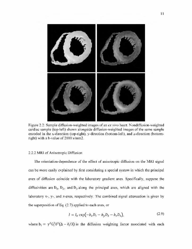
reduced. One method to attain higher b-values while minimizing the effects of motion is
to use stimulated-echo acquisition mode (STEAM) based acquisition in conjunction with
twice cardiac-gating, where the excitation and re-excitation, or first and third, RF pulses
are synchronized to the cardiac cycle [74], as seen in Fig. 2.9. Even with halved SNR
A
Figure 2.9: Stimulated-echo acquisition mode (STEAM) pulse sequence. The diffusion sensitizing gradients are highlighted in grey. The first and third RF pulses are synchronized to occur at the same time point in the cardiac cycle. Using STEAM allows for higher b-values given a fixed gradient strength, but at the cost of losing half of the acquired signal due to using a stimulated-echo.

associated with using stimulated echoes, the approach has been found effective in
mitigating motion and is increasingly used in DTI studies in humans and large animals
[80], [108], [109]. Regardless of the means for compensation, the heightened sensitivity
of diffusion MRI makes motion extremely challenging to correct and leaves very little
room for uncorrected instrument imperfections.
Second, even if the images are free of motion artifacts, motion of the heart can lead to
erroneous estimates due to the strain-memory effect of the diffusion constants. Strain
alters the relative distance between any two given points of a tissue. Because the
diffusion-weighted MRI signal is derived in part based on the probability of spatial
displacement, strain can add or subtract from the displacement, and lead to over or under
estimation of the diffusion measurements. The effects of strain on in vivo cardiac DTI
measurements have long been documented [76]. Because cardiac strain can be separately
quantified via, for example, tagged MRI, its effects can be subtracted to obtain pure
diffusion and fiber orientation measurements from in vivo cardiac DTI data [76].
Moreover, because the effects depend on the average strain across the cardiac cycle, it
has been shown possible to obtain strain-free in vivo cardiac DTI measurements by
selecting the right timing delay in the cardiac-gated acquisition [77].
Lastly, recent advances in gradient hardware technology have made high-strength
gradients available (up to 80 mT/m in whole-body scanners and 1500 mT/m or more in
small animal systems as of the current writing), which in turn made it practically feasible
to employ bipolar encoding gradient pulses capable of generating moderate but sufficient
b-values, in terms of diffusion encoding, in diffusion MRI and DTI, including for cardiac
imaging [110]. Bipolar diffusion pulses offer not only reduced motion sensitivity, as
37

described in the above section, they also have decreased memory effects of strain [108].
However, besides the impact on accuracy as explained in Section 2.4.2, using the
relatively low b-values associated with bipolar gradient pulses can also inadvertently
introduce effects of tissue perfusion and lead to additional error in the DTI experiment.
Perfusion, in this case blood flow in the capillary bed, has long been known for causing
additional spin phase dispersion and leading to overestimated diffusion coefficients via
the so called intravoxel incoherent motion (IVIM) effect [111] in highly vascularized
organs such as the liver [112]. Because the capillary flow is faster than the diffusion of
water, the flow-mediated perfusion effect can be eliminated from diffusion measurements
by employing sufficiently high (b > 200 s/mm2) diffusion weighting. The perfusion
dependence of diffusion MRI has been theorized [111], [113] and recently empirically
demonstrated [114] for the perfused heart.
Together, it is clear that the specific physiology of the heart adds technical issues that
need to be considered in performing in vivo cardiac DTI. Despite technological advances
that have made most the known issues tractable, complete understanding and
compensating the effects of motion in cardiac DTI remain works in progress. In the
meantime, caution is warranted in interpreting in vivo cardiac DTI results.
2.5 Accelerating DTI Acquisition
Because of its minimum dataset requirement, and the frequent use of signal
averaging, including increasing the number of encoding gradient directions, to improve
its accuracy, practical applications of DTI have been hampered by long scan times. Due
to the repetitive nature of the DTI experiment, reduction or elimination of redundancies
38

in the data has been explored as a potential means to accelerate the data acquisition [102].
The so-called compressed sensing is an advanced technique that reconstructs MRI images
from partially sampled data [115], [116]. The relative benefits of compressed sensing are
demonstrated in Fig. 2.10. Conventional reconstructions, using direct inverse Fourier
transform for example, of partially sampled k-space data often lead to structured artifacts
such as blurring and ringing in the result images. One key feature of compressed sensing
is randomized k-space sampling, which turns the effects of partial k-space sampling into
incoherent, noise-like artifacts. The latter are then minimized to yield images close to
what the fully sampled k-space would have achieved, but using data that were acquired in
39
Helix Angle FA
- 90 ° 0 ° 90 ° 0 0.25 0.5Figure 2.10. FA and helix angle maps from accelerated DTI data. Helix angle and fractional anisotropy (FA) maps from (first row) using all acquired data or the “Gold- standard” case reconstructed traditionally and (second row) using 1/16th of the acquired data, reconstructed using the model-based compressed sensing reconstruction.

a fraction of the time.
The ideal experiment for applying compressed sensing is one where some knowledge
of the images to be reconstructed already exists. In general, compressed sensing
reconstruction can be formulated as the minimization of some cost function given in the
form of
C(m) = ||F(m) - y ||! + a ||^ (m )|li, (216)
—* 2where ||F(m) — y|| is the data fidelity term and ||^ (m )|\1 is the image sparsifying term.
The fidelity term is akin to the least squares fitting between the acquired signal, y, and the
estimated image, m , transformed into the measurement domain, or k-space, by the
undersampled Fourier operator F(-). The image sparsifying term is used to drive the
estimated image, m, to have desired features, such as spatial smoothness or sparsity,
using a transform, ^ . Common examples of image sparsifying transforms are the total
variation (TV) and wavelet transforms. The estimated image, m, is reconstructed by
minimizing Eq. (2.16) with respect to m
m = minm||F(m) - y||^ + a ||^ (m )|\t , (217)
which is performed using a numerical method such as gradient descent or conjugate
gradient. The contributions from the data fidelity and image sparsifying terms are
controlled by the regularizing term, a.
DTI lends itself well to compressed sensing because of the redundancies across the
diffusion-weighted images (e.g., same organ size and shape with only diffusion contrast
differences). The general cost function in Eq. (2.16) can be altered to include the series of
diffusion-weighted images [117]
40

N
C(mn) = ^ ( | | F ( m n) - y||^ + ll^(mn)lll) . (218)n = l
The reconstructed individual diffusion-weighted images, mn, can then be used to
obtain the diffusion tensors similar to the standard DTI experiment. The goal of such
reconstructions is to acquire DTI data in a reduced amount of time without incurring the
proportional loss in accuracy associated with the scan time acceleration.
2.6 Conclusion
Considering that the heart is active since before birth and for the most part throughout
a person’s life, myocardial microstructure changes across orders of magnitude in both
time and space making structural measurements rather challenging. This short contextual
survey of structural measurements via MR-DTI hopefully illustrates a versatile response
to this challenge. Now, it is worth mentioning some promising examples of the future of
fiber structure acquisition, and how it can have a positive effect in the way we understand
cardiac structure and function. Despite its complexity, fiber structure is intimately linked
to diagnosing, monitoring, and treating heart disease, which is one of the largest causes of
death in the world. For this reason, many researchers and clinicians recognize the value
of applying understanding of the heart on personalized medicine. This ideal includes two
fundamental layers, the characterization of functional and material parameters in health
and disease, as well as predicting the outcome of an intervention on a patient. The first
layer involves gathering large databases of relevant information, including anatomical
and diffusion tensor imaging, and establishing analysis criteria useful for classifying
phenotypes and recognizing disease [118], [119]. Such an approach, would endow
clinicians with information-age diagnostic tools never before seen [120]. Much of the
41

42
statistical machinery, such as the ability to merge large amounts of tensor images, is
already been applied to the brain to the classification of adult and developing structures
[121], [122], and their cardiac counterparts are underway [123]. Likewise, thanks to
advances in computational cardiology, the ability of predicting the outcomes of treatment
is no longer a dream. Computational models are becoming an important tool for planning
therapeutic strategies for fibrillation [124], and for the prevention of side effects, like
venous occlusion by pacemaker lead placement [125]. With the advent of more
comprehensive approaches, like electro-mechanical models of the whole heart and the
ability to acquire fiber structure information in vivo, predicting the outcome of surgical
procedures is within sight. Despite all the technical and logistical complexities, the hope
of improving the quality of life of millions is a permanent source of encouragement for
researchers, engineers, clinicians, as well as any of those willing to answer relevant
questions in cardiac biomechanics including characterizing cardiac fiber structure.

43
2.7 References
[1] L. K. Waldman, D. Nosan, F. Villarreal, and J. W. Covell, “Relation betweentransmural deformation and local myofiber direction in canine left ventricle,” Circ. Res., vol. 63, no. 3, pp. 550-62, Sep. 1988.
[2] P. H. M. Bovendeerd, T. Arts, J. M. Huyghe, D. H. van Campen, and R. S.Reneman, “Dependence of local left ventricular wall mechanics on myocardial fiber orientation: a model study,” J. Biomech., vol. 25, no. 10, pp. 1129-40, Oct. 1992.
[3] L. Garrido, V. J. Wedeen, K. K. Kwong, U. M. Spencer, and H. L. Kantor,“Anisotropy of water diffusion in the myocardium of the rat,” Circ. Res., vol. 74, no. 5, pp. 789-793, May 1994.
[4] T. Arts, F. W. Prinzen, L. H. Snoeckx, J. M. Rijcken, and R. S. Reneman,“Adaptation of cardiac structure by mechanical feedback in the environment of the cell: a model study,” Biophys. J., vol. 66, no. 4, pp. 953-961, 1994.
[5] L. Geerts, P. H. M. Bovendeerd, K. Nicolay, and T. Arts, “Characterization of thenormal cardiac myofiber field in goat measured with MR-diffusion tensor imaging,” Am. J. Physiol. Heart Circ. Physiol., vol. 283, pp. H139-45, Jul. 2002.
[6] P.-S. Chen, Y.-M. Cha, B. B. Peters, and L. S. Chen, “Effects of myocardial fiberorientation on the electrical induction of ventricular fibrillation,” Am. J. Physiol. Circ. Physiol., vol. 264, pp. H1760-H1773, 1993.
[7] D. F. Scollan, A. Holmes, R. Winslow, and J. Forder, “Histological validation ofmyocardial microstructure obtained from diffusion tensor magnetic resonance imaging,” Am. J. Physiol., vol. 275, no. 6, pp. H2308-18, Dec. 1998.
[8] J. D. Humphrey, Cardiovascular Solid Mechanics. Springer, 2002, p. 776.
[9] Y. C. Fung, Biomechanics: Mechanical Properties of Living Tissues, SecondEdition, 2nd ed. New York, US: Springer, 2004, p. 568.
[10] A. D. McCulloch, “Cardiac Biomechanics,” in The Biomedical EngineeringHandbook, 2nd Editio., J. Bronzino, Ed. Boca Raton: CRC Press, 2000, pp. 28-46.
[11] J. M. Guccione, Computational Cardiovascular Mechanics: Modeling andApplications in Heart Failure. Springer, 2010, p. 348.
[12] R. H. Clayton, O. Bernus, E. M. Cherry, H. Dierckx, F. H. Fenton, L. Mirabella, A.V Panfilov, F. B. Sachse, G. Seemann, and H. Zhang, “Models of cardiac tissue electrophysiology: progress, challenges and open questions,” Prog. Biophys. Mol. Biol., vol. 104, no. 1-3, pp. 22-48, 2011.
[13] L. Clerc, “Directional Differences of Impulse Spread in Trabecular Muscle fromMammalian Heart,” J Physiol, vol. 255, pp. 335-346, 1976.
44
[14] D. E. Roberts, L. T. Hersh, and A. M. Scher, “Influence of cardiac fiber orientationon wavefront voltage, conduction velocity, and tissue resistivity in the dog,” Circ. Res., vol. 44, no. 5, pp. 701-12, May 1979.
[15] F. B. Sachse, Computational Cardiology: Modeling of Anatomy, Electrophysiology,and Mechanics, 1st ed. New York, US: Springer, 2004, p. 322.
[16] P. J. Hunter, A. D. McCulloch, and H. E. ter Keurs, “Modelling the mechanicalproperties of cardiac muscle,” Prog. Biophys. Mol. Biol., vol. 69, pp. 289-331, Jan. 1998.
[17] P. Schmid, T. Jaermann, P. Boesiger, P. F. Niederer, P. P. Lunkenheimer, C. W.Cryer, and R. H. Anderson, “Ventricular myocardial architecture as visualised in postmortem swine hearts using magnetic resonance diffusion tensor imaging,” Eur. J. Cardiothorac. Surg., vol. 27, no. 3, pp. 468-72, Mar. 2005.
[18] A. Fick, “Ueber Diffusion,” Ann. Phys., vol. 170, no. 1, pp. 59-86, 1855.
[19] A. Einstein, Investigations on the Theory of Brownian Motion, reprint of the 1stEnglish edition (1926). Dover, New-York, 1956.
[20] H. C. Torrey, “Bloch Equations with Diffusion Terms,” Phys. Rev., vol. 104, no. 3,pp. 563-565, 1956.
[21] E. O. Stejskal and J. E. Tanner, “Spin Diffusion Measurements: Spin Echoes in thePresence of a Time-Dependent Field Gradient,” J. Chem. Phys., vol. 42, no. 1, p. 288, 1965.
[22] P. J. Basser, J. Mattiello, and D. LeBihan, “Estimation of the Effective SelfDiffusion Tensor from the NMR Spin Echo,” J. Magn. Reson. B, vol. 103, pp. 24725, 1994.
[23] P. J. Basser, J. Mattiello, and D. LeBihan, “MR diffusion tensor spectroscopy andimaging,” Biophys J, vol. 66, no. 1, pp. 259-67, Jan. 1994.
[24] P. J. Basser and D. K. Jones, “Diffusion-tensor MRI: theory, experimental designand data analysis - a technical review,” NMR Biomed., vol. 15, pp. 456-67, 2002.
[25] J. Mattiello, P. J. Basser, and D. LeBihan, “Analytical Expressions for the b Matrixin NMR Diffusion Imaging and Spectroscopy,” J. Magn. Reson. A, vol. 108, pp. 131-141, 1994.
[26] E. W. Hsu, A. L. Muzikant, S. A. Matulevicius, R. C. Penland, and C. S. Henriquez,“Magnetic resonance myocardial fiber-orientation mapping with direct histological correlation,” Am. J. Physiol., vol. 274, no. 5, pp. H1627-34, May 1998.
[27] A. A. Holmes, D. F. Scollan, and R. L. Winslow, “Direct histological validation ofdiffusion tensor MRI in formaldehyde-fixed myocardium,” Magn Reson Med, vol.

45
44, no. 1, pp. 157-61, Jul. 2000.
[28] I. J. LeGrice, P. J. Hunter, B. H. Smaill, and B. H. Smailll, “Laminar structure of theheart: a mathematical model,” Am. J. Physiol. Circ. Physiol., vol. 272, no. 5, pp. H2466-H2476, 1997.
[29] S. H. Gilbert, D. Benoist, A. P. Benson, E. White, S. F. Tanner, A. V Holden, H. Dobrzynski, O. Bernus, and A. Radjenovic, “Visualization and quantification of whole rat heart laminar structure using high-spatial resolution contrast-enhanced MRI,” Am. J. Physiol. Heart Circ. Physiol., vol. 302, no. 1, pp. H287-98, Jan. 2012.
[30] P. A. Helm, H.-J. Tseng, L. Younes, E. R. McVeigh, and R. L. Winslow, “Ex vivo3D diffusion tensor imaging and quantification of cardiac laminar structure,” Magn Reson Med, vol. 54, no. 4, pp. 850-9, Oct. 2005.
[31] Y. Jiang, K. Pandya, O. Smithies, and E. W. Hsu, “Three-dimensional diffusiontensor microscopy of fixed mouse hearts,” Magn. Reson. Med., vol. 52, no. 3, pp. 453-60, Sep. 2004.
[32] D. Rohmer, A. Sitek, and G. T. Gullberg, “Reconstruction and visualization of fiberand laminar structure in the normal human heart from ex vivo diffusion tensor magnetic resonance imaging (DTMRI) data,” Invest. Radiol., vol. 42, no. 11, pp. 777-89, Nov. 2007.
[33] W.-Y. I. Tseng, V. J. Wedeen, T. G. Reese, R. N. Smith, and E. F. Halpern,“Diffusion tensor MRI of myocardial fibers and sheets: correspondence with visible cut-face texture,” J. Magn. Reson. Imaging, vol. 17, no. 1, pp. 31-42, Jan. 2003.
[34] D. F. Scollan, a Holmes, J. Zhang, and R. L. Winslow, “Reconstruction of cardiacventricular geometry and fiber orientation using magnetic resonance imaging,” Ann. Biomed. Eng., vol. 28, no. 8, pp. 934-44, Aug. 2000.
[35] Y. Jiang, J. M. Guccione, M. B. Ratcliffe, and E. W. Hsu, “Transmural heterogeneityof diffusion anisotropy in the sheep myocardium characterized by MR diffusion tensor imaging,” Am. J. Physiol. Heart Circ. Physiol., vol. 293, no. 4, pp. H2377- 84, Oct. 2007.
[36] L. J. Healy, Y. Jiang, and E. W. Hsu, “Quantitative comparison of myocardial fiberstructure between mice, rabbit, and sheep using diffusion tensor cardiovascular magnetic resonance,” J. Cardiovasc. Magn. Reson., vol. 13, no. 1, p. 74, Jan. 2011.
[37] P. A. Helm, L. Younes, M. F. Beg, D. B. Ennis, C. Leclercq, O. P. Faris, E.McVeigh, D. Kass, M. I. Miller, and R. L. Winslow, “Evidence of structural remodeling in the dyssynchronous failing heart,” Circ. Res., vol. 98, no. 1, pp. 12532, Jan. 2006.
[38] J. C. Walker, J. M. Guccione, Y. Jiang, P. Zhang, A. W. Wallace, E. W. Hsu, and M.

46
B. Ratcliffe, “Helical myofiber orientation after myocardial infarction and left ventricular surgical restoration in sheep,” J. Thorac. Cardiovasc. Surg., vol. 129, pp. 382-90, Feb. 2005.
[39] J. Chen, W. Liu, H. Zhang, L. Lacy, X. Yang, S. Song, S. A. Wickline, X. Yu, andX. Y. Re-, “Regional ventricular wall thickening reflects changes in cardiac fiber and sheet structure during contraction : quantification with diffusion tensor MRI,” Am. J. Physiol. Heart Circ. Physiol., vol. 289, pp. H1898-H1907, 2005.
[40] P. P. Lunkenheimer, K. Redmann, N. Kling, X. Jiang, K. Rothaus, C. W. Cryer, F.Wubbeling, P. Niederer, P. U. Heitz, S. Y. Ho, and R. H. Anderson, “Threedimensional architecture of the left ventricular myocardium,” Anat. Rec. A. Discov. Mol. Cell. Evol. Biol., vol. 288, no. 6, pp. 565-78, Jun. 2006.
[41] J. H. Omens, H. A. Rockman, J. W. Covell, H. Jeffrey, and A. Rockman, “Passiveventricular mechanics in tight-skin mice Passive ventricular mechanics in tight-skin mice,” Am J Physiol Hear. Circ Physiol, vol. 266, pp. H1169-H1176, 1994.
[42] A. A. Young, I. J. LeGrice, M. A. Young, and B. H. Smaill, “Extended confocalmicroscopy of myocardial laminae and collagen network,” J. Microsc., vol. 192, no. Pt 2, pp. 139-50, Nov. 1998.
[43] P. Schmid, P. P. Lunkenheimer, K. Redmann, K. Rothaus, X. Jiang, C. W. Cryer, T.Jaermann, P. Niederer, P. Boesiger, and R. H. Anderson, “Statistical analysis of the angle of intrusion of porcine ventricular myocytes from epicardium to endocardium using diffusion tensor magnetic resonance imaging,” Anat. Rec., vol. 290, no. 11, pp. 1413-23, Nov. 2007.
[44] M. Smerup, E. Nielsen, P. Agger, J. Frandsen, P. Vestergaard-Poulsen, J. Andersen,J. Nyengaard, M. Pedersen, S. Ringgaard, V. Hjortdal, P. P. Lunkenheimer, and R.H. Anderson, “The three-dimensional arrangement of the myocytes aggregated together within the mammalian ventricular myocardium,” Anat. Rec., vol. 292, no.I, pp. 1-11, Jan. 2009.
[45] E. W. Hsu, D. L. Buckley, J. D. Bui, S. J. Blackband, and J. R. Forder, “Two-component diffusion tensor MRI of isolated perfused hearts,” Magn. Reson. Med., vol. 45, no. 6, pp. 1039-45, Jun. 2001.
[46] M. T. Wu, W. I. Tseng, M. Y. Su, C. P. Liu, K. R. Chiou, V. J. Wedeen, T. G.Reese, and C. F. Yang, “Diffusion tensor magnetic resonance imaging mapping the fiber architecture remodeling in human myocardium after infarction: correlation with viability and wall motion,” Circulation, vol. 114, no. 10, pp. 1036-45, Sep.2006.
[47] D. E. Sosnovik, R. Wang, G. Dai, T. Wang, E. Aikawa, M. Novikov, A.Rosenzweig, R. J. Gilbert, and V. J. Wedeen, “Diffusion spectrum MRI tractography reveals the presence of a complex network of residual myofibers in infarcted myocardium,” Circ. Cardiovasc. Imaging, vol. 2, no. 3, pp. 206-12, May

47
2009.
[48] S. Zhang, J. A. Crow, X. Yang, J. Chen, A. Borazjani, K. B. Mullins, W. Chen, R. C.Cooper, R. M. McLaughlin, and J. Liao, “The correlation of 3D DT-MRI fiber disruption with structural and mechanical degeneration in porcine myocardium,” Ann. Biomed. Eng., vol. 38, no. 10, pp. 3084-95, Oct. 2010.
[49] M.-T. Wu, W.-Y. I. Tseng, M.-Y. Su, C.-P. Liu, K.-R. Chiou, V. J. Wedeen, T. G.Reese, and C.-F. Yang, “Diffusion tensor magnetic resonance imaging mapping the fiber architecture remodeling in human myocardium after infarction: correlation with viability and wall motion,” Circulation, vol. 114, no. 10, pp. 1036-45, Sep. 2006.
[50] E. X. Wu, Y. Wu, J. M. Nicholls, J. Wang, S. Liao, S. Zhu, C.-P. P. Lau, and H.-F.F. Tse, “MR diffusion tensor imaging study of postinfarct myocardium structural remodeling in a porcine model,” Magn. Reson. Med., vol. 58, no. 4, pp. 687-95, Oct. 2007.
[51] E. X. Wu, Y. Wu, H. Tang, J. Wang, J. Yang, M. C. Ng, E. S. Yang, C. W. Chan, S.Zhu, C.-P. Lau, and H.-F. Tse, “Study of myocardial fiber pathway using magnetic resonance diffusion tensor imaging,” Magn Reson Med, vol. 25, no. 7, pp. 1048-57, Sep. 2007.
[52] M. J. Collins, T. Ozeki, J. Zhuo, J. Gu, R. Gullapalli, R. N. Pierson, B. P. Griffith, P.W. M. Fedak, and R. S. Poston, “Use of diffusion tensor imaging to predict myocardial viability after warm global ischemia: possible avenue for use of nonbeating donor hearts,” J. Heart Lung Transplant., vol. 26, no. 4, pp. 376-83, Apr.2007.
[53] B. Schmitt, K. Fedarava, J. Falkenberg, K. Rothaus, N. K. Bodhey, C. Reischauer, S.Kozerke, B. Schnackenburg, D. Westermann, P. P. Lunkenheimer, R. H. Anderson, F. Berger, and T. Kuehne, “Three-dimensional alignment of the aggregated myocytes in the normal and hypertrophic murine heart,” pp. 921-927, 2009.
[54] G. J. Strijkers, A. Bouts, W. M. Blankesteijn, T. H. J. M. Peeters, A. Vilanova, M. C.van Prooijen, H. M. H. F. Sanders, E. Heijman, and K. Nicolay, “Diffusion tensor imaging of left ventricular remodeling in response to myocardial infarction in the mouse,” NMR Biomed, vol. 22, no. 2, pp. 182-90, Feb. 2009.
[55] S. Huang and D. E. Sosnovik, “Molecular and Microstructural Imaging of the Myocardium,” Curr. Cardiovasc. Imaging Rep., vol. 3, no. 1, pp. 26-33, Feb. 2010.
[56] I. J. LeGrice, Y. Takayama, and J. W. Covell, “Transverse shear along myocardialcleavage planes provides a mechanism for normal systolic wall thickening,” Circ. Res., vol. 77, no. 1, pp. 182-193, 1995.
[57] P. P. Lunkenheimer, K. Redmann, P. Niederer, P. Schmid, M. Smerup, J. Stypmann,S. Dabritz, K. Rothaus, and R. H. Anderson, “Models versus established knowledge

48
in describing the functional morphology of the ventricular myocardium,” Heart Fail. Clin., vol. 4, no. 3, pp. 273-88, Jul. 2008.
[58] R. H. Anderson, D. Sanchez-Quintana, K. Redmann, and P. P. Lunkenheimer, “Howare the myocytes aggregated so as to make up the ventricular mass?” Semin. Thorac. Cardiovasc. Surg. Pediatr. Card. Surg. Annu., pp. 76-86, Jan. 2007.
[59] C. M. Kramer, “Insights into myocardial microstructure during infarct healing andremodeling: pathologists need not apply,” Circ. Cardiovasc. Imaging, vol. 2, no. 1, pp. 4-5, Jan. 2009.
[60] F. Vadakkumpadan, H. Arevalo, A. J. Prassl, J. Chen, F. Kickinger, P. Kohl, G.Plank, and N. Trayanova, “Image-based models of cardiac structure in health and disease,” Wiley Interdiscip. Rev. Syst. Biol. Med., vol. 2, no. 4, pp. 489-506, 2010.
[61] J. F. Wenk, K. Sun, Z. Zhang, M. Soleimani, L. Ge, D. Saloner, A. W. Wallace, M.B. Ratcliffe, and J. M. Guccione, “Regional left ventricular myocardial contractility and stress in a finite element model o f posterobasal myocardial infarction,” J. Biomech. Eng., vol. 133, no. 4, p. 044501, Apr. 2011.
[62] S. G. Campbell and A. D. McCulloch, “Multiscale computational models of familialhypertrophic cardiomyopathy: genotype to phenotype,” J. R. Soc. Interface, vol. 8, no. 64, pp. 1550-61, Nov. 2011.
[63] P. H. M. Bovendeerd, “Modeling of cardiac growth and remodeling of myofiberorientation,” J. Biomech., vol. 45, no. 5, pp. 872-81, Mar. 2012.
[64] J. Chen, S. K. Song, W. Liu, M. McLean, J. S. Allen, J. Tan, S. A. Wickline, and X.Yu, “Remodeling of cardiac fiber structure after infarction in rats quantified with diffusion tensor MRI,” Am. J. Physiol. Heart Circ. Physiol., vol. 285, no. 3, pp. H946-54, Sep. 2003.
[65] C. M. Ripplinger, W. Li, J. Hadley, J. Chen, F. Rothenberg, R. Lombardi, S. A.Wickline, A. J. Marian, and I. R. Efimov, “Enhanced transmural fiber rotation and connexin 43 heterogeneity are associated with an increased upper limit o f vulnerability in a transgenic rabbit model of human hypertrophic cardiomyopathy,” Circ. Res., vol. 101, no. 10, pp. 1049-57, Nov. 2007.
[66] Y. Wu and E. X. Wu, “MR investigation of the coupling between myocardial fiberarchitecture and cardiac contraction,” Conf. Proc. IEEE Eng. Med. Biol. Soc., vol.2009, pp. 4395-8, Jan. 2009.
[67] J. Rijcken, T. Arts, P. H. M. Bovendeerd, B. Schoofs, D. Van Campen, and others,“Optimization of left ventricular fibre orientation of the normal heart for homogeneous sarcomere length during ejection,” Eur. J. Morphol., vol. 34, no. 1, pp. 39-46, 1996.
[68] J. Rijcken, P. H. M. Bovendeerd, A. J. G. Schoofs, D. H. van Campen, and T. Arts,

49
“Optimization of cardiac fiber orientation for homogeneous fiber strain during ejection,” Ann. Biomed. Eng., vol. 27, no. 3, pp. 289-97, 1999.
[69] D. B. Ennis, T. C. Nguyen, J. C. Riboh, L. Wigstrom, K. B. Harrington, G. T.Daughters, N. B. Ingels, and D. C. Miller, “Myofiber angle distributions in the ovine left ventricle do not conform to computationally optimized predictions,” J. Biomech., vol. 41, no. 15, pp. 3219-24, Nov. 2008.
[70] J. C. Walker, M. B. Ratcliffe, P. Zhang, A. W. Wallace, B. Fata, E. W. Hsu, D.Saloner, and J. M. Guccione, “MRI-based finite-element analysis of left ventricular aneurysm,” Am. J. Physiol. Heart Circ. Physiol., vol. 289, no. 2, pp. H692-700, Aug. 2005.
[71] J. C. Walker, M. B. Ratcliffe, P. Zhang, A. W. Wallace, E. W. Hsu, D. a Saloner,and J. M. Guccione, “Magnetic resonance imaging-based finite element stress analysis after linear repair of left ventricular aneurysm,” J. Thorac. Cardiovasc. Surg., vol. 135, no. 5, pp. 1094-102, 1102.e1-2, May 2008.
[72] C. Mekkaoui, S. Huang, H. H. Chen, G. Dai, T. G. Reese, W. J. Kostis, A.Thiagalingam, P. Maurovich-Horvat, J. N. Ruskin, U. Hoffmann, M. P. Jackowski, and D. E. Sosnovik, “Fiber architecture in remodeled myocardium revealed with a quantitative diffusion CMR tractography framework and histological validation,” J. Cardiovasc. Magn. Reson., vol. 14, no. 1, p. 70, Jan. 2012.
[73] W. I. Tseng, J. Dou, T. G. Reese, and V. J. Wedeen, “Imaging myocardial fiberdisarray and intramural strain hypokinesis in hypertrophic cardiomyopathy with MRI,” J. Magn. Reson. Imaging, vol. 23, no. 1, pp. 1-8, Jan. 2006.
[74] R. R. Edelman, J. Gaa, V. J. Wedeen, E. Loh, J. M. Hare, P. Prasad, and W. Li, “Invivo measurement of water diffusion in the human heart,” Magn. Reson. Med., vol. 32, no. 3, pp. 423-8, Sep. 1994.
[75] T. G. Reese, R. M. Weisskoff, R. N. Smith, B. R. Rosen, R. E. Dinsmore, and V. J.Wedeen, “Imaging myocardial fiber architecture in vivo with magnetic resonance,” Magn. Reson. Med., vol. 34, no. 6, pp. 786-791, 1995.
[76] T. G. Reese, V. J. Wedeen, and R. M. Weisskoff, “Measuring Diffusion in thePresence of Material Strain,” J. Magn. Reson. B, vol. 112, no. 3, pp. 253-8, Sep.1996.
[77] W. I. Tseng, T. G. Reese, R. M. Weisskoff, and V. J. Wedeen, “Cardiac diffusiontensor MRI in vivo without strain correction,” Magn. Reson. Med., vol. 42, pp. 393-403, 1999.
[78] W. I. Tseng, T. G. Reese, R. M. Weisskoff, T. J. Brady, and V. J. Wedeen,“Myocardial fiber shortening in humans: initial results of M R imaging,” Radiology, vol. 216, no. 1, pp. 128-39, Jul. 2000.

50
[79] J. Dou, W. I. Tseng, T. G. Reese, and V. J. Wedeen, “Combined diffusion and strainMRI reveals structure and function of human myocardial laminar sheets in vivo,” Magn. Reson. Med., vol. 50, no. 1, pp. 107-13, Jul. 2003.
[80] M.-T. Wu, M.-Y. M. Su, Y.-L. Huang, K.-R. Chiou, P. Yang, H.-B. Pan, T. G.Reese, V. J. Wedeen, and W.-Y. I. Tseng, “Sequential changes of myocardial microstructure in patients postmyocardial infarction by diffusion-tensor cardiac MR: correlation with left ventricular structure and function,” Circ. Cardiovasc. Imaging, vol. 2, no. 1, pp. 32-40, 6 p following 40, Jan. 2009.
[81] T. Q. Li, a M. Takahashi, T. Hindmarsh, and M. E. Moseley, “ADC mapping bymeans of a single-shot spiral MRI technique with application in acute cerebral ischemia,” Magn Reson Med, vol. 41, no. 1, pp. 143-7, Jan. 1999.
[82] C. Liu, R. Bammer, D.-H. Kim, and M. E. Moseley, “Self-navigated interleavedspiral (SNAILS): application to high-resolution diffusion tensor imaging,” Magn Reson Med, vol. 52, no. 6, pp. 1388-96, Dec. 2004.
[83] D. Le Bihan, R. Turner, and J. R. MacFall, “Effects of intravoxel incoherent motions(IVIM) in steady-state free precession (SSFP) imaging: application to molecular diffusion imaging,” Magn. Reson. Med., vol. 10, no. 3, pp. 324-37, Jun. 1989.
[84] J. A. McNab and K. L. Miller, “Sensitivity of diffusion weighted steady state freeprecession to anisotropic diffusion,” Magn. Reson. Med., vol. 60, no. 2, pp. 405-13, Aug. 2008.
[85] J. G. Pipe, V. G. Farthing, and K. P. Forbes, “Multishot Diffusion-Weighted FSEUsing PROPELLER MRI,” Magn. Reson. Med., vol. 52, pp. 42-52, 2002.
[86] S. Skare, R. D. Newbould, D. B. Clayton, and R. Bammer, “Propeller EPI in theother direction,” Magn. Reson. Med., vol. 55, no. 6, pp. 1298-307, Jun. 2006.
[87] K. P. Pruessmann, M. Weiger, M. B. Scheidegger, and P. Boesiger, “SENSE:sensitivity encoding for fast MRI,” Magn Reson Med, vol. 42, no. 5, pp. 952-62, Nov. 1999.
[88] M. A. Griswold, P. M. Jakob, R. M. Heidemann, M. Nittka, V. Jellus, J. Wang, B.Kiefer, and A. Haase, “Generalized Autocalibrating Partially Parallel Acquisitions ( GRAPPA ),” Magn Reson Med, vol. 47, no. 6, pp. 1202-1210, Jun. 2002.
[89] S. J. Holdsworth, S. Skare, R. D. Newbould, and R. Bammer, “Robust GRAPPA-accelerated diffusion-weighted readout-segmented (RS)-EPI,” Magn Reson Med, vol. 62, no. 6, pp. 1629-1640, Dec. 2009.
[90] K.-D. Merboldt, W. Hanicke, H. Bruhn, M. L. Gyngell, and J. Frahm, “DiffusionImaging of the Human Brain in Vivo,” Magn. Reson. Med., vol. 23, pp. 179-192, 1992.

51
[91] R. Bammer, S. J. Holdsworth, W. B. Veldhuis, and S. T. Skare, “New methods inDiffusion Weighted and Diffusion Tensor Imaging,” Magn Reson Imaging Clin N Am, vol. 17, no. 2, pp. 175-204, 2009.
[92] B. Chen and E. W. Hsu, “Noise removal in magnetic resonance diffusion tensorimaging,” Magn Reson Med, vol. 54, no. 2, pp. 393-401, Aug. 2005.
[93] P. J. Basser and S. Pajevic, “Statistical artifacts in diffusion tensor MRI (DT-MRI)caused by background noise,” Magn. Reson. Med., vol. 44, no. 1, pp. 41-50, Jul. 2000.
[94] D. K. Jones, M. A. Horsfield, and A. Simmons, “Optimal strategies for measuringdiffusion in anisotropic systems by magnetic resonance imaging,” Magn. Reson. Med., vol. 42, no. 3, pp. 515-25, Sep. 1999.
[95] L. R. Frank, “Anisotropy in high angular resolution diffusion-weighted MRI,” MagnReson Med, vol. 45, no. 6, pp. 935-9, Jun. 2001.
[96] D. S. Tuch, T. G. Reese, M. R. Wiegell, N. Makris, J. W. Belliveau, and V. J.Wedeen, “High angular resolution diffusion imaging reveals intravoxel white matter fiber heterogeneity,” Magn Reson Med, vol. 48, no. 4, pp. 577-82, Oct.2002.
[97] D. A. Xing, N. G. Papadakis, C. L.-H. Huang, V. M. Lee, T. Adrian Carpenter, andL. D. Hall, “Optimised diffusion-weighting for measurement of apparent diffusion coefficient (ADC) in human brain,” Magn Reson Med, vol. 15, no. 7, pp. 771-784,1997.
[98] D. C. Alexander and G. J. Barker, “Optimal imaging parameters for fiber-orientationestimation in diffusion MRI,” Neuroimage, vol. 27, no. 2, pp. 357-67, Aug. 2005.
[99] C. G. Koay, L.-C. Chang, J. D. Carew, C. Pierpaoli, and P. J. Basser, “A unifyingtheoretical and algorithmic framework for least squares methods of estimation in diffusion tensor imaging,” J. Magn. Reson., vol. 182, no. 1, pp. 115-25, Sep. 2006.
[100] L. Bao, Y. Zhu, W. Liu, M. Robini, Z. Pu, and I. Magnin, “Analysis of cardiac diffusion tensor magnetic resonance images using sparse representation,” Conf. Proc. IEEE Eng. Med. Biol. Soc., vol. 2007, pp. 4516-9, Jan. 2007.
[101] L. Bao, Y. M. Zhu, W. Y. Liu, P. Croisille, Z. B. Pu, M. Robini, and I. E. Magnin, “Denoising human cardiac diffusion tensor magnetic resonance images using sparse representation combined with segmentation,” Phys. Med. Biol., vol. 54, no. 6, pp. 1435-56, Mar. 2009.
[102] E. W. Hsu and C. S. Henriquez, “Myocardial fiber orientation mapping using reduced encoding diffusion tensor imaging,” J Cardiov Magn Reson, vol. 3, no. 4, pp. 339-47, Jan. 2001.

52
[103] C. Frindel, M. Robini, S. Rapacchi, E. Stephant, Y. Zhu, and P. Croisille, “Towards In Vivo Diffusion Tensor MRI on Human Heart using Edge-Preserving Regularization,” Proc. 29th Annu. Int. Conf. IEEE EMBS Cite Int. Lyon, Fr., pp. 6007-6010, 2007.
[104] C. L. Welsh, E. V. R. Dibella, G. Adluru, and E. W. Hsu, “Model-based reconstruction of undersampled diffusion tensor k-space data,” Magn Reson Med, vol. 70, pp. 429-440, Sep. 2013.
[105] S. Rapacchi, H. Wen, P. Kellman, and V. M. Pai, “Low b-Value Diffusion- Weighted Cardiac Magnetic,” vol. 46, no. 12, pp. 751-758, 2011.
[106] A. J. de Crespigny, M. P. Marks, D. R. Enzmann, and M. E. Moseley, “Navigated Diffusion Imaging of Normal and Ischemic Human Brain,” Magn. Reson. Med., vol. 33, no. 5, pp. 720-728, 1995.
[107] S. Nielles-Vallespin, C. Mekkaoui, P. Gatehouse, T. G. Reese, J. Keegan, P. F. Ferreira, S. Collins, P. Speier, T. Feiweier, R. de Silva, M. P. Jackowski, D. J. Pennell, D. E. Sosnovik, and D. Firmin, “In vivo diffusion tensor MRI of the human heart: Reproducibility of breath-hold and navigator-based approaches,” Magn Reson Med, pp. 1-12, Oct. 2012.
[108] J. Dou, T. G. Reese, W. I. Tseng, and V. J. Wedeen, “Cardiac diffusion MRI without motion effects,” Magn. Reson. Med., vol. 48, no. 1, pp. 105-14, Jul. 2002.
[109] S. Nielles-Vallespin, C. Mekkaoui, P. Gatehouse, T. G. Reese, J. Keegan, P. F. Ferreira, S. Collins, P. Speier, T. Feiweier, R. de Silva, M. P. Jackowski, D. J. Pennell, D. E. Sosnovik, and D. Firmin, “In vivo diffusion tensor MRI of the human heart: reproducibility of breath-hold and navigator-based approaches,” Magn. Reson. Med., vol. 70, no. 2, pp. 454-464, Sep. 2013.
[110] U. Gamper, P. Boesiger, and S. Kozerke, “Diffusion imaging of the in vivo heart using spin echoes--considerations on bulk motion sensitivity,” Magn. Reson. Med., vol. 57, no. 2, pp. 331-7, Feb. 2007.
[111] D. Le Bihan, E. Breton, D. Lallemand, M.-L. Aubin, J. Vignaud, and M. Laval- Jeantet, “Separation of Diffusion and Perfusion in Intravoxel Incoherent Motion MR Imaging,” Radiology, vol. 168, no. 2, pp. 497-505, 1988.
[112] A. Luciani, A. Vignaud, M. Cavet, J. T. Van Nhieu, A. Mallat, L. Ruel, A. Laurent, J.-F. Deux, P. Brugieres, and A. Rahmouni, “Liver Cirrhosis : Intravoxel Incoherent Motion MR Imaging — Pilot Study,” Radiology, vol. 249, pp. 891-899, 2008.
[113] D. Le Bihan and R. Turner, “The capillary network: a link between IVIM and classical perfusion,” Magn. Reson. Med., vol. 27, no. 1, pp. 171-178, Sep. 1992.
[114] O. Abdullah, A. D. Gomez, O. Stedham, M. Heideinger, S. Poelzing, and E. W. Hsu, “Effects of Perfusion on Cardiac MR Diffusion Measurements,” in

53
Proceedings of the 21st Annual Meeting of ISMRM, 2013.
[115] D. L. Donoho, “Compressed sensing,” IEEE T Inf. Theory, vol. 52, no. 4, pp. 1289-1306, Apr. 2006.
[116] M. Lustig, D. Donoho, and J. M. Pauly, “Sparse MRI: The application of compressed sensing for rapid MR imaging,” Magn Reson Med, vol. 58, no. 6, pp. 1182-95, Dec. 2007.
[117] G. Adluru, E. Hsu, and E. V. R. DiBella, “Constrained reconstruction of sparse cardiac MR DTI data,” LNCS, vol. 4466, pp. 91-99, 2007.
[118] J. V Tu, S. E. Brien, C. C. Kennedy, L. Pilote, and W. A. Ghali, “Introduction to the Canadian Cardiovascular Outcomes Research Team’s (CCORT) Canadian Cardiovascular Atlas project,” Can. J. Cardiol., vol. 19, no. 3, pp. 225-9, Mar.2003.
[119] C. G. Fonseca, M. Backhaus, D. A. Bluemke, R. D. Britten, J. Do Chung, B. R. Cowan, I. D. Dinov, J. P. Finn, P. J. Hunter, A. H. Kadish, D. C. Lee, J. A. C. Lima, P. Medrano-Gracia, K. Shivkumar, A. Suinesiaputra, W. Tao, and A. A. Young, “The Cardiac Atlas Project--an imaging database for computational modeling and statistical atlases of the heart,” Bioinformatics, vol. 27, pp. 2288-95, Aug. 2011.
[120] N. A. Trayanova, T. O’Hara, J. D. Bayer, P. M. Boyle, K. S. McDowell, J. Constantino, H. J. Arevalo, Y. Hu, and F. Vadakkumpadan, “Computational cardiology: how computer simulations could be used to develop new therapies and advance existing ones,” Europace, vol. 14 Suppl 5, pp. v82-v89, Nov. 2012.
[121] H. Huang, “Delineating neural structures of developmental human brains with diffusion tensor imaging,” ScientificWorldJournal., vol. 10, pp. 135-44, Jan. 2010.
[122] Z. Cui, S. Zhong, P. Xu, Y. He, and G. Gong, “PANDA: a pipeline toolbox for analyzing brain diffusion images,” Front. Hum. Neurosci., vol. 7, p. 42, Jan. 2013.
[123] N. Toussaint, M. Sermesant, C. T. Stoeck, S. Kozerke, and P. G. Batchelor, “In vivo human 3D cardiac fibre architecture: reconstruction using curvilinear interpolation o f diffusion tensor images,” Med. Image Comput. Comput. Assist. Interv., vol. 13, pp. 418-25, Jan. 2010.
[124] K. S. McDowell, F. Vadakkumpadan, R. Blake, J. Blauer, G. Plank, R. S. MacLeod, and N. A. Trayanova, “Methodology for patient-specific modeling o f atrial fibrosis as a substrate for atrial fibrillation,” J. Electrocardiol., vol. 45, no. 6, pp. 640-5, 2012.
[125] A. Lonyai, A. M. Dubin, J. A. Feinstein, C. A. Taylor, and S. C. Shadden, “New insights into pacemaker lead-induced venous occlusion: simulation-based investigation of alterations in venous biomechanics,” Cardiovasc. Eng., vol. 10, no. 2, pp. 84-90, Jun. 2010.

CHAPTER 3
MODEL-BASED RECONSTRUCTION OF UNDERSAMPLED
DIFFUSION TENSOR K-SPACE DATA1
3.1 Abstract
The practical utility of diffusion tensor imaging, especially for 3D high-resolution
spin warp experiments of ex vivo specimens, has been hampered by long acquisition
times. To accelerate the acquisition, a compressed sensing framework that uses a model-
based formulation to reconstruct diffusion tensor fields from undersampled k-space data
was presented and evaluated. Accuracies in brain specimen white matter fiber orientation,
fractional anisotropy, and mean diffusivity mapping were compared with alternative
methods achievable using the same scan time via reduced image resolution, fewer
diffusion encoding directions, standard compressed sensing, or asymmetrical sampling
reconstruction. The efficiency of the proposed approach was also compared with fully
sampled cases across a range of the number of diffusion encoding directions. In general,
the proposed approach was found to reduce the image blurring and noise and to provide
more accurate fiber orientation, fractional anisotropy, and mean diffusivity measurements
1 © 2012 Wiley Periodicals, Inc. Reprinted, with permission, from Christopher Lee Welsh, Edward V.R. DiBella, Ganesh Adluru, and Edward W. Hsu. Model-Based Reconstruction of Undersampled Diffusion Tensor k-Space Data. Magnetic Resonance in Medicine. DOI 10.1002/mrm.24486.

compared with the alternative methods. Moreover, depending on the degree of
undersampling used and the diffusion tensor imaging parameter examined, the
measurement accuracy of the proposed scheme was equivalent to fully sampled diffusion
tensor imaging datasets that consist of 33-67% more encoding directions and require
proportionally longer scan times. The findings show model-based compressed sensing to
be promising for improving the resolution, accuracy, or scan time of diffusion tensor
imaging.
3.2 Introduction
Diffusion tensor imaging [1] (DTI) is an MRI technique that allows quantitative
characterization of the geometry and organization of tissue microstructures such as fiber
orientation. DTI has been applied in the brain [2], [3] to, for example, trace white matter
tracts [4]-[6], map connectivity, and characterize damage caused by stroke [7]-[9]. The
method has also been applied to ex vivo specimens of the heart [10]-[12] to map
structural changes due to fibrosis or infarction [13]-[17].
Because the diffusion tensor is a rank 2, symmetric matrix [1], a unique solution of
the diffusion tensor requires a minimum of six diffusion-weighted images sensitized in
noncollinear diffusion encoding directions, plus a nondiffusion-weighted image. In this
sense, the minimum scan time required for a DTI dataset, which spans both the spatial
and diffusion dimensions, is seven times that of an anatomical scan acquired using the
same sequence and settings. DTI suffers from low signal-to-noise ratio (SNR) because
diffusion is measured as signal attenuation and from increased echo time necessary to
accommodate the use of diffusion sensitizing gradients. In practice, the loss of signal is
55

often compensated for by additional signal averaging in forms of acquisition repetition or
increasing the number of encoding directions, which further prolongs the scan time.
Consequently, methods to accelerate the acquisition, especially those that minimize
further SNR loss, are highly desirable.
Perhaps the most obvious method to accelerate acquisition would be to either scan at
a lower resolution or simply encode fewer diffusion directions. Scanning at a lower
resolution would introduce blurring and make it more difficult to discern fine structures
in an image. In contrast, although the resolution is maintained, encoding in fewer
diffusion directions would sacrifice the accuracy of the diffusion tensor estimation. A
possible solution to both of these problems is to accelerate acquisition by partially
sampling k-space, and apply reconstruction in such a way that fine structure and diffusion
tensor accuracy are preserved. When not reconstructed properly, partially sampling k-
space introduces artifacts in image space, such as ghosting, field-of-view overlap, or
additional noise, depending on the undersampling pattern used. Techniques have been
introduced to reduce the effects of partial sampling or undersampling when DTI is
acquired using multiple receive coils [18]-[23].
Rather than reconstructing each image of the multi-image acquisition separately,
compressed sensing techniques [24]-[26] are capable of jointly estimating multiple
acquisitions by sharing sparsely sampled data. Compressed sensing can be particularly
attractive for DTI, due to the high degree of similarity or redundancy (e.g., the size and
shape of the brain, including the white matter) among the acquisitions at different
diffusion directions that can be leveraged to represent a transform of the data sparsely.
Previously, compressed sensing based on undersampling in the diffusion encoding or q-
56

space has been applied to high-angular-resolution diffusion imaging [27], [28], which is a
more general form of diffusion imaging that allows resolution of crossing fibers. A
possible alternate way to undersample DTI or high-angular-resolution diffusion imaging
data is in k-space [29] or spatial frequency domain. Intuitively, the nature of the desired
information in the DTI dataset and the well-known relationship between image-space and
k-space may offer flexibility that can be exploited for effective undersampling. For
example, the fiber orientation of the brain white matter or myocardium varies relatively
slowly and, therefore, the relevant information can be captured even when the outer k-
space is sampled with a lower density.
Regardless of the scheme of undersampling, it is important that the performance of
any reconstruction method be evaluated on not only the acquisition time acceleration, but
also on its ability to capture the desired information. In DTI, fiber orientation, fractional
anisotropy (FA) [30], and mean diffusivity (MD) are the often sought-after parameters
for assessing tissue microstructure. Therefore, ideally the performance of any compressed
sensing acceleration needs to be evaluated in terms of accuracy loss in measuring these
parameters with respect to a ‘‘ground truth’’ or ‘‘gold standard.’’ Moreover, to be
considered effective, any proposed technique should retain more accuracy than
alternative methods using, for example, lower resolution or fewer diffusion encoding
directions to achieve the same acceleration.
The goal of the current study is to investigate the validity of a compressed sensing
framework for DTI that, in addition, uses the signal intensity model to directly estimate
diffusion tensor fields from undersampled k-space data. The formulation bypasses the
usual intermediate step of estimating diffusion-weighted images. By estimating the
57
diffusion tensor directly, the number of variables to be solved is reduced from N x
d im l xdim 2 xdim 3 to 6 x d im l xdim 2 xdim 3 (excluding the nonweighted volume)
where dim1, dim2, and dim3 are the spatial dimensions of a 3D acquisition, and N is the
number of diffusion-weighted images acquired. In a noise-dominated system, reducing
the number of unknowns can provide the more accurate estimates of the fitted
parameters. As well, the model-based formulation provides a convenient platform that
numerous practical considerations involved in DTI (e.g., phase errors) can be addressed
in a single step. Model-based approaches have been proposed previously to compensate
for eddy currents, field inhomogeneities, and motion in DTI [31], [32] and to reconstruct
diffusion tensor tomography data [33] but not for accelerating acquisition. Other
compressed sensing techniques using exponential models have been proposed for T1 and
T2 mapping [34], [35].
The current model-based algorithm is demonstrated on a 3D DTI acquisition, which
is used for high-resolution characterization of fixed specimens [36], [37]. Three
dimensional DTI, especially one acquired with a spin-echo sequence, can take many
hours for ex vivo acquisitions and thus can benefit greatly from acquisition acceleration.
Also, 3D acquisitions have a higher degree of data redundancy and can be undersampled
in more than one dimension. For the sake of brevity, in the following sections, and unless
otherwise noted, the term DTI strictly refers to 3D spin-warp spin-echo DTI. The
effectiveness of the model-based compressed sensing algorithm is validated against other
means to achieve comparable scan time reduction. Part o f the current work has been
presented previously in a conference abstract [38].
58

59
3.3 Theory
Compressed sensing finds the target images by subjecting the estimates to a set of
reconstruction constraints and minimization of the associated penalty or cost function.
One form of a cost function for compressed sensing [24], [39] reconstruction of a series
of N undersampled MRI k-space data, dn, is given as:
where || ||2 represents the L2-norm, which produces the least squares solution [25] and
can be substituted by any other type of measure of deviation between images [40], and
m n is the estimated magnitude images. The terms m n and dn are the vectorized versions
of m n and dn, such that for image resolution dim1 by dim2, the vectors m n and dn have
dim1 x dim2 elements. The first term in Eq. (3.1) is a fidelity term that forces the solution
to adhere to the acquired k-space data. The second term in Eq. (3.1) is a total variation
(TV) operator [41] applied in image space to constrain the solution to generate piecewise-
constant images, hence reducing erratic points due to undersampling k-space. The scalar
regularization weight factor a controls the relative contributions of the fidelity and TV
terms. The jth k-space element of the k-space signal model, F(mn, n ) , is
where Wn is the binary undersampling function for the diffusion direction n, is the
image phase which is estimated and fixed from the acquired low-resolution data from
each diffusion-weighted image, x is the position in image space, and kj is the position in
k-space. The series of images, m n, can be obtained simultaneously by minimizing the
Fj(mn, n) = Wn( k j mn(x) • • e 1 x'^i (3.2)

cost function in Eq. (3.1) with respect to m n.
In the current model-based DTI reconstruction, to allow direct estimation of the
diffusion tensor, m n is replaced with the standard diffusion tensor intensity model [1].
This allows direct estimation of the diffusion tensor. The relationship between mn and
the DTI signal is given by,
m n = l0 e - b9lDgn (3.3)
where I0 is the image without diffusion weighting, b is the diffusion weighting factor and
gn = (gxn, gyn, gzn)T is the diffusion encoding directional vector in the 3D space
spanned by the readout (x), phase (y), and slice (z) encoding directions. D is the rank 2,
symmetric tensor defined as:
60
Dxx Dxy DxzD = Dxy Dy" (3.4)
Dxz Dyy Dzz_
Replacing m n yields the new k-space signal model:
Fj(D,n) = Wn(kj) ^ /0(x) • e~h& D(! Bn • • e -! (3.5)X
For the current formulation, the TV term can be defined as:
7V (0 ) = || J ( m j ! + ( m j ! || (3 6)
where (mn)y and (mn) z are the partial derivatives of m n with respect to y and z. TV is
not calculated in the x-direction since it is already fully-sampled.
Maps corresponding to each diffusion tensor element can be estimated by minimizing
Eq. (3.1) simultaneously with respect to each element of the tensor, D, via, for example,
gradient descent optimization. To perform gradient descent, computational equations for
the derivative of Eq. (3.1) are needed with respect to each diffusion tensor element,

61
Ds (s G {xx, yy, zz, xy, xz, y z }).
3 C ( D)
dD, = £ - 2 H 9 „ 9 ! sI oe - b̂ D° " R e a l \ e ( F ^ D , n ) - djn ) e ! ! !
n=l V !
h( ^ ~ ______ Cmn) y_______\ _______(fflj!_______\9n9n s n ygy ^ 2 + p i ) d z y j 2 + ( ^ J 2 + p i )
(3.7)
where gng^ is a 3 x 3 matrix and the (0 s operator extracts the sth element corresponding
to the Ds parameter map. The full derivation of this equation can be found in the attached
appendix. The diffusion tensor elements are then updated iteratively using the derivative
in Eq. (3.7):
D l+1 = D! - A (38)
where A is the step size used in the gradient descent and r is the iteration number.
3.4 Methods
3.4.1 Dataset
Fully sampled 3D, Cartesian k-space, DTI spin-echo data consisting of diffusion-
weighted scans in a relatively high number of encoding directions (96 in all) and four
nondiffusion-weighted “b0” images (100 x 75 x 70 matrix size, 0.5 x 0.5 x 0.5 mm3
isotropic voxel size, echo time (TE) = 39 ms, repetition time (TR) = 500 ms, and number
of excitations (NEX) = 1) were acquired on a fixed, excised macaque brain hemisphere
using a Bruker Biospec 7T scanner (Bruker Biospin Inc., Billerica, MA) equipped with a
high-performance gradient system (max gradient amplitude capable of 600 mT/m). The
acquisition time for the entire diffusion MRI dataset was ~72 h. Figure 3.1 shows the
‘‘b0’’ and diffusion-weighted images of a representative 2D slice, for reference. The

62
Figure 3.1: Two-dimensional MRI coronal view of the macaque brain hemisphere used in this study. Left, nondiffusion-weighted “b0” image, b = 0 s/mm2 . Right, diffusion- weighted image, b = 5000 s/mm2 in a single diffusion direction, scaled up for better display. There is notable shading due to coil inhomogeneity.
diffusion tensor solution to the entire fully sampled dataset was used as the gold standard
for subsequent performance assessments.
3.4.2 Undersampling Schemes
To simulate more typical DTI acquisitions, 10 test datasets each composed of a subset
of diffusion-weighted images encoded in 24 gradient directions were retrospectively
selected from the original 96-direction set. The first direction of each subset was
randomly chosen, and the remaining directions were selected based on maximizing the
angular distance between each successive encoding direction [42]. To have distinct
datasets, precaution was taken to avoid excessive overlap of gradient directions between
any two datasets. When the gradient directions overlapped by more than 45%, alternative
gradient directions were substituted. Among the final test datasets, the amount of overlap
ranged from 8 to 45%, with 20% being the average.

Undersampling was subsequently applied to the above test datasets, which was
mathematically equivalent to multiplying the k-space data with appropriate binary masks.
k-Space was undersampled in the phase (y) and slice (z) directions, whereas sampled
fully in the readout (x) direction for the 3D data. Two different degrees of undersampling
were examined, 50 and 75%, which are equal to the acceleration factor R of 2 and 4,
respectively. Figure 3.2 shows examples of the binary masks used with R of 2 and 4. To
take advantage of the low-frequency nature of DTI data, the center k-space was fully
sampled, whereas the remaining k-space was sampled randomly, using a uniform
distribution, to achieve the desired overall acceleration factor. The reference image, I0,
was sampled fully and reconstructed separately using an inverse Fourier transform. The
reference image was fixed throughout the reconstruction.
3.4.3 Reconstruction
All computation was performed using Matlab (Mathworks, Natick, Mass; version
R2011a). Two steps were taken in preparation for the iterative compressed sensing
reconstruction. First, an inverse Fourier transform was applied to the k-space data along
the readout direction, which were fully sampled. The procedure permitted the
reconstruction of data in each subsequent 2D ky-kz plane perpendicular to the readout
direction to be performed separately and in parallel. Second, the phase map, needed in
Eq. (3.5) was approximated from the central fully sampled k-space block and low-pass
filtered using a 2D Hann window.
Implementation o f the compressed sensing reconstruction is summarized in the
flowchart shown in Fig. 3.3. The estimation was initialized by the linear least squares
63

64
Figure 3.2: Two-dimensional representation of sampling masks in the phase-slice plane for 50% (left) and 75% (right) undersampling. The data were sampled fully in the readout direction.
fit o f the diffusion tensor to the images generated by direct reconstruction (inverse
Fourier transform) o f the undersampled k-space data. The initialization o f the diffusion
tensor is important, but the optimization solution can withstand a wide range o f initial
conditions (e.g., initializing DTI parameters to the tensor solution of using the b0 image
plus identical DWIs). The algorithm then enters a loop, the first step of which is to
determine the derivative o f the cost function with respect to each o f the diffusion
coefficients, according to the procedure outlined in the Theory section. A value of
1 x 1 0 _6 was used for b in Eq. (3.7). The derivatives were used to update the diffusion
tensor elements according to Eq. (3.8). The loop was repeated until convergence was
achieved, which was determined to occur when the value of the cost function changed by
less than 1x 10_4 from iteration to iteration.
Optimal values of the computational parameters, TV weight a, and step size A from
Eqs. (3.7) and (3.8) were determined empirically by reconstructing an arbitrarily selected
test dataset with a range of values of a and A. The values that yielded the most

65
Figure 3.3: Flowchart of the model-based reconstruction algorithm.
accurate tensor eigenvector estimation with respect to the gold standard, 0.00025 and
0.00001 for a and A, respectively, were used in the remaining test datasets. The
parameters were found to be relatively robust and when changed by a factor of 10,
increased the estimation errors by only about 10%. The reconstruction of each
undersampled 24-direction test dataset typically converged within 1000 iterations and
took ~1.0 h on a computer with a quad-core processor, 8 GB of RAM, and Matlab’s
Parallel-Computing toolbox.
3.4.4 Assessment of Performance
The effectiveness of the proposed model-based compressed sensing DTI technique
was evaluated by comparing its performance to those of two other reconstruction
techniques and two control experiments all of which required equal total scan time:
1. Conventional compressed sensing. The compressed sensing reconstruction
individual diffusion-weighted images by minimizing the cost function defined in
Eq. (3.1) with respect to m n, as in [29], utilizing a TV weight, a, equal to 0.025,
and performing 300 iterations. The data were undersampled in the same manner
as the proposed model-based approach.
2. Asymmetrical sampling. In the asymmetrical sampling case, a modified

iterative partial Fourier method [43] was used to fill in the missing k-space. k-
Space was sampled asymmetrically in the phase (k y ) direction to get an overall
acceleration factor, R, of 2 and 4. Ten phase-encodes of negative k-space were
sampled for R = 2 and five phase encodes for R = 4. To maintain the same
acceleration factor as the other techniques, the same number of phase-encoding
steps were not sampled at the high, positive frequencies, but were estimated in the
reconstruction to maintain the original resolution.
3. Low resolution. In the lower resolution control scheme, the center half (which
is 1/V 2 in each phase and slice dimensions for R = 2) or center fourth (1 /2 in
each phase and slice dimensions for R = 4) of k-space for each test dataset was
taken and zero- padded. The diffusion-weighted images were obtained by using
the inverse Fourier transform.
4. Fewer directions. The fewer directions control scheme used fewer encoding
directions to achieve the same R factor (12 and 6 fully encoded images for R = 2
and R = 4, respectively). The directions used for R = 2 and 4 were found by
iterating over every 12- and 6-direction combination in each 24-direction test
dataset to find the combination that minimized the fiber orientation deviation
angle for each test dataset. Again, the diffusion-weighted images were obtained by
using the inverse Fourier transform.
In each of the reconstruction and control experiments, the diffusion tensors and their
derived parameters were obtained using conventional means (linear least squares fitting
on a pixel-by-pixel basis).
The performances of the acquisition schemes in capturing the essential DTI
66

information were quantified along three error metrics: the fiber orientation deviation
angle (A0, in degrees), fractional anisotropy difference (AFA, dimensionless), and MD
difference (AMD, cm2/s) with respect to the gold standard. Fiber orientation, fractional
anisotropy, and MD are parameters commonly derived from DTI results, which are useful
in tractography and detection of pathology. The fiber deviation angle, A0, was calculated
by finding the angular difference (arccosine o f the vector dot product) between primary
eigenvectors o f the gold standard and the model-based estimate. A0 was averaged over
the brain white matter, which was defined as regions with FA greater than 0.3. In low FA
areas, such as the brain gray matter, where diffusion is relatively isotropic, noise can lead
to wide fluctuations of the primary eigenvector and skew the error metric. In contrast,
root-mean square (RMS) of the FA difference, AFA, and MD difference, AMD, were
calculated over the entire specimen. The mean A0, RMS AFA, and RMS AMD metrics
obtained for the proposed and alternate schemes in all 10 test datasets were compared
using one-way repeated measurement analysis o f variance. When significant group
difference (i.e., F-test with P < 0.05) was found, post-hoc multiple comparisons based on
the Bonferroni criterion with overall P < 0.005 were conducted to identify the group
pairings that were significantly different.
Whereas the above comparisons were intended largely to assess the relative
advantages of the proposed scheme, to offer guidance in the design of future DTI studies,
and as an alternative way to evaluate the performance, it is instructive to determine the
fully sampled DTI experiment that offers equivalent performance as the proposed
scheme. To this end, the performance metrics, mean A0 and RMS AFA, were obtained as
described above for DTI experiments that comprised fully sampled diffusion-weighted
67

images encoded over a range of the number of gradient directions (N, 6 < N < 24, 10
experiments for each N ). The DTI experiments (i.e., N ) that yielded the same
performances as the proposed schemes for each R = 2 and R = 4 case were then
identified. As an additional reference, the performance metrics obtained for N= 24 were
extrapolated to lower values of N via the 1/VN relationship, which approximated DTI
experiments that are SNR limited. The same analysis was not carried out for AMD
because the deviations were found to be small across all schemes and, therefore,
improving its measurement efficiency was less critical.
3.5 Results
Figure 3.4 shows the FA-weighted, red-green-blue (RGB) color-coded primary
eigenvector maps for the model- based, compressed sensing, asymmetrical, low-
resolution, and fewer direction cases, for R = 2 and 4, obtained for a representative test
dataset. Qualitatively, compared with the gold standard (also shown in Fig. 3.4), all five
schemes produced progressively worse DTI maps as the acceleration factor R increased,
which was expected. The limitations of each of the low-resolution and fewer directions
control schemes were more conspicuous at R = 4. There was considerable blurring in the
low-resolution scheme, whereas the noise was markedly higher in the reduced direction
scheme. In contrast, the issues were clearly improved or avoided in the model-based
compressed sensing approach.
Figure 3.5 shows the MD maps for the five test cases. The degradation in quality due
to image acceleration was less apparent for the MD maps than it was for the FA maps
shown in the previous figure, although there was more blurring in the low-resolution
68
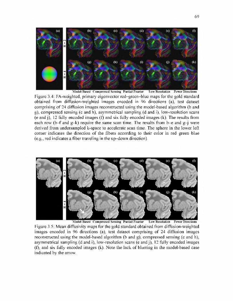
69
(b) (c)jr r
l / V t y
. (d) I (e) I ( / * * \ / > - l y l / l y
i ■ . . j i ■ . ■ ' “
4 L ' * * , ,
A l, / v i, j ' A i k A * F f \
~Js£ > K K ' H *Model-Based Compressed Sensing Partial Fourier Low Resolution Fewer Directions
Figure 3.4: FA-weighted, primary eigenvector red-green-blue maps for the gold standard obtained from diffusion-weighted images encoded in 96 directions (a), test dataset comprising of 24 diffusion images reconstructed using the model-based algorithm (b and g), compressed sensing (c and h), asymmetrical sampling (d and i), low-resolution scans (e and j), 12 fully encoded images (f) and six fully encoded images (k). The results from each row (b -f and g-k) require the same scan time. The results from b-e and g-j were derived from undersampled k-space to accelerate scan time. The sphere in the lower left corner indicates the direction of the fibers according to their color in red-green-blue (e.g., red indicates a fiber traveling in the up-down direction).
Model-Based Compressed Sensing Partial Fourier Low Resolution Fewer Directions
Figure 3.5: Mean diffusivity maps for the gold standard obtained from diffusion-weighted images encoded in 96 directions (a), test dataset comprising of 24 diffusion images reconstructed using the model-based algorithm (b and g), compressed sensing (c and h), asymmetrical sampling (d and i), low-resolution scans (e and j), 12 fully encoded images (f), and six fully encoded images (k). Note the lack of blurring in the model-based case indicated by the arrow.

scheme than in the model-based case. The MD maps had more in common with each
other than did the FA maps.
The above qualitative observations are supported by the histograms of the
performance metrics shown in Fig. 3.6, for the same test dataset. In each R = 2 and R = 4
case, the distributions of A9, AFA, and AMD for the model-based compressed sensing
scheme were generally not only narrower but also closer to zero, compared with those of
70
- • - L o w - Resolution • Fewer Directions -M odel-Based -Compressed Sensing -Asymmetrical Sampling[
0 10 20 30Primary Eigenvector Deviation (deg)
Figure 3.6: Distribution of primary eigenvector (top row), FA (middle row), and mean diffusivity deviation (bottom row) for 50% (left) and 75% (right) undersampling for the same test dataset shown in Figs. 3.4 and 3.5. The model-based approach (solid squares) was compared against compressed sensing (solid diamonds) and asymmetrical reconstructions (solid triangles) and comparable low-resolution (dashed circles) and fewer direction (dash dot x ’s) cases. The bias in FA deviation (e.g., in the fewer directions case for R = 4) indicates that the FA was underestimated when compared with the gold standard.

the other reconstruction and control schemes, with the exception of AMD in the fewer
directions case. An exception to the observed trends in the histograms was in the R = 4
case, where the A9 distributions between the proposed and low-resolution schemes were
similar. However, this may be due to the noise-smoothing effect inherent to lowering the
scan resolution and the absence of a penalty for blurring in the performance metrics. The
similarity likely reflects artifacts of the experimental methodology, and not actual
benefits of the low-resolution scheme. Also, there appears
to be a slight bias in AFA for the proposed model-based technique, the cause of which is
currently unclear.
The quantitative performance comparisons among the schemes are summarized in
Tables 3.1 and 3.2, which contain the means of A9, AFA, and AMD for each R = 2 and R
= 4 case, respectively. Once again, the results were consistent with the above qualitative
observations. Among the test datasets examined, the model-based approach at R = 2
produced a mean A9 of 4.11 ± 0.05° (n = 10, ± SEM), RMS AFA of 3.22 ± 0.07 x 10'2
and RMS AMD of 1.09 ± 0.01 x 10⁻⁷ cm2/s, which were better than those, respectively,
71
Table 3.1. Performance of DTI acceleration schemes in terms of fiber orientation, FA, and MD errors for an acceleration Factor R = 2
Metrics
SchemesMean A6 (°)
RMS AFA (10-2)
RMS AMD(10-7 cm2/s)
Model-based 4.11 ± 0.05 3.22 ± 0.07 1.09 ± 0.01Compressed Sensing 4.81 ± 0.06 3.98 ± 0.06 1.18 ± 0.01Asymmetrical sampling 4.77 ± 0.07 4.12 ± 0.07 3.58 ± 0.03Low resolution 4.83 ± 0.06 3.98 ± 0.05 1.88 ± 0.01Fewer Directions 4.93 ± 0.12 4.35 ± 0.01 0.57 ± 0.03
Entries are mean ± SEM for the 10 test datasets examined.

72
Table 3.2. Performance of DTI acceleration schemes in terms of fiber orientation, FA, and MD Errors for an acceleration factor R = 4
Metrics
SchemesMean A9 (°)
RMS AFA (10-2)
RMS AMD(10-7 cm2/s)
Model-based 6.63 ± 0.04 4.86 ± 0.07 1.90 ± 0.02Compressed Sensing 7.74 ± 0.04 5.71 ± 0.04 2.27 ± 0.01Asymmetrical sampling 8.05 ± 0.08 6.00 ± 0.05 3.73 ± 0.02Low resolution 7.17 ± 0.04 5.43 ± 0.03 2.93 ± 0.01Fewer Directions 8.89 ± 0.14 7.22 ± 0.03 0.89 ± 0.05
Entries are mean ± SEM for the 10 test datasets examined.
obtained by compressed sensing and asymmetrical reconstructions and the low-resolution
scheme. The model-based approach performed better than the fewer direction case in
terms of mean A9 and RMS AFA (4.93 ± 0.12° and 4.35 ± 0.01 x 10⁻²) but not RMS
AMD (0.57 ± 0.03 x 10⁻⁷ cm2/s). Similarly, at R = 4, the proposed scheme outperformed
the compressed sensing and asymmetrical reconstructions and, again, the low-resolution
scheme and the fewer direction scheme in terms of mean A9 and RMS AFA (8.89 ± 0.14°
and 7.22 ± 0.03 x 10⁻²) but not RMS AMD (0.89 ± 0.05 x 10⁻⁷ cm2/s).
Figure 3.7 shows the results of the repeated measurement analysis of variance post
hoc comparisons. The results indicate that the performance of the proposed model-based
compressed sensing scheme, in terms of A9 and AFA, was significantly better than any of
the other reconstruction or control methods. Moreover, between the two control schemes,
lowering the scan resolution performs significantly better, in terms of mean A9 and RMS
AFA, than reducing the number of diffusion encoding directions in all cases except for
mean A9 at R = 2. Again, this may be due to the noise-smoothing effect of lowering the
scan resolution. Nevertheless, the results point out that, for a given total scan time, more

73
CD<1ccc0)
<u.<3C/i
SC£
Qs<1C/5£02
MBCSASLRFD
MBCSASLRFD
MBCSPFASFD
R = 2(50% Undersam pling)
R = 4(75% Undersam pling)
MB CS AS LR FD MB CS AS LR FD
Figure 3.7. Results of pairwise, post hoc analysis of the five DTI acceleration schemes from Tables 3.1 and 3.2. Asterisks denote a significant difference between the pairs, which was determined by P < 0.005 for each post hoc comparison by Bonferroni criterion. MB, model-based; CS, compressed sensing; AS, asymmetrical sampling; LR, low resolution; and FD, fewer directions. The model-based approach was shown to be statistically different from the other four acceleration approaches.
relevant DTI information was captured by the proposed model-based compressed sensing
scheme than by realizing the acquisition acceleration via reducing the scan resolution or
the number of diffusion encoding directions.
The results of the diffusion encoding gradient direction number and equivalent
model-based reconstructed DTI experiment analysis are illustrated in Fig. 3.8, from
which several observations can be made. First, in general and as expected, the number of
diffusion encoding directions was inversely proportional to the error. Second, as the
number of diffusion encoding directions was reduced from 24, AFA closely follows the
performance of a noise-dominated DTI experiment where the RMS AFA error metric was
proportional to (VN)_1. However, mean A9 deviates more from the (VN)_1 curve,

74
10
O)Q)
X !
LU_Q)O)C<
-•-M o d e l-B a s e d— Fewer Directions- - Noise Estimate
% 1'V - a%
* %, 1
ll
0.08
LU<LL
CODC
0.06
0.04
10 15 20 # of encoding directions
25 0.
v ^% \
- • -M o d e l-B a s e d— Fewer Directions- - Noise Estimate\ X\ a
-«----■iiii
i "lI
iiii
025 10 15 20# of encoding directions
25
Figure 3.8. DTI fiber orientation (left) and FA (right) measurement errors plotted as a function of the scan time in terms of the number of fully sampled diffusion scans included in the dataset. The dash-dotted lines represent the 1/V N dependence of the errors based on the 24-direction case. The performances of the proposed model-based approach are plotted at their equivalent scan times, and are extrapolated (dotted lines) to determine the number of fully encoded diffusion-weighted images needed to achieve the same measurement accuracy.
suggesting that the accuracy of the diffusion tensor eigenvector (the fiber orientation) can
easily suffer from unoptimized placements of the diffusion encoding gradient directions.
Third, at low numbers of gradient directions (<9), both mean A9 and RMS AFA
dramatically depart from the noise-dominated behavior. Finally, depending on the
reduction factor R used and the DTI parameter being measured, the proposed model-
based compressed sensing scheme can achieve performances that are equivalent to a
longer DTI experiment using a higher number of gradient directions. Specifically, instead
of a DTI experiment using fully sampled diffusion-weighted images encoded in 12
gradient directions, using a nominal R = 2 to encode in 24 gradient directions in the same
acquisition time, the proposed scheme would produce equivalent fiber orientation
accuracy that is otherwise achievable by a longer DTI scan using 16 gradient directions.
In the case of FA mapping, the accuracy is equivalent to using 20 gradient directions.
Similarly, instead of a six-direction fully sampled DTI acquisition, using a nominal R = 4

to encode in 24 gradient directions, the proposed model-based approach would produce
equivalent fiber orientation and FA mapping accuracy of six- and nine-direction fully
sampled DTI experiments, respectively.
3.6 Discussion
The results from this study show that the proposed model-based compressed sensing
approach for DTI was generally more accurate and produces less blurring than spatial TV
compressed sensing and iterative asymmetrical reconstruction methods. Also, the
proposed method was better for fiber orientation and FA estimation than either the lower
resolution or fewer direction control experiments of equal scan time, as seen in Fig. 3.6.
These trends are shown quantitatively in Tables 3.1 and 3.2, and are statistically
significant (Fig. 3.7). Combined, these results demonstrate the validity of the proposed
approach for accelerating DTI, obtaining more accurate DTI, or a combination of both.
One possible exception to the relative performance of the proposed scheme was in the
AMD metric when compared with the fewer direction control case, where the deviation
7 7 2of the former was about twice that of the latter (1.09 x 10' vs. 0.57 x 10' cm /s, for R =
2). It is noted that both AMD values represent only 1-2% deviation from the actual MD
value for the entire specimen (0.58 x 10⁻⁵ cm2/s). In contrast, the percentages of AFA
values of the same schemes (3.22 x 10⁻² and 4.35 x 10⁻²) were an order of magnitude
larger, or about 15% of the whole-specimen FA (0.26). Moreover, unlike all other
schemes examined, the fewer direction scheme was based on datasets that were unaltered
image subsets of the gold standard. The overlap of image data would have made not only
the AMD error but also the AFA error artificially lower than its true value, but the effect
75

was less apparent because of the larger error associated with AFA. Combined, the
observed AMDs for the fewer direction control scheme as seen in Figs. 3.5 and 3.6 and
Tables 3.1 and 3.2 were likely artificial underestimations of already low deviation values.
The data undersampling and scan time savings afforded by the model-based
reconstruction can be exploited to include more DTI diffusion encoding gradient
directions. Typically, DTI using more encoding directions is better than simply signal
averaging in the same directions, especially when the number of directions used is
relatively low [44]. The proposed compressed sensing technique in effect allows more
DTI encoding directions to be used without requiring a proportional increase in the scan
time. A second factor that contributed to the performance of the proposed approach was
in its use of model-based reconstruction, where fewer parameters were involved in the
estimation. When the model-based DTI estimation was applied to the nonundersampled
test datasets (data not shown), the mean A9 and RMS AFA performance metrics improved
from 3.23° and 3.01 x 10⁻² to 2.77° and 2.48 x 10⁻², respectively. Although spatial
smoothing, such as in the case of lower resolution scans, can produce artificially
improved metrics, it is unlikely that the model-based compressed sensing method added
smoothing, since a very low weighting factor a = 0.00025 was used for the spatial TV
constraint in Eq. (3.7). As well, in Fig. 3.4, the model-based result contained little or no
evidence of blurring.
Practical implications of the current work for designing DTI acquisition schemes can
be extrapolated from the results summarized in Fig. 3.8. With either R = 2 or 4
undersampling, the proposed approach was equivalent to fully sampled DTI scans using
1.33 (8/6 for R = 4 or 16/12 for R = 2) times more encoding directions, in terms of the
76

required scan time and the performance in fiber orientation mapping. For FA mapping,
the equivalence factors were even greater, 1.5 (or 9/6) and 1.67 (or 20/12) at R = 4 and R
= 2, respectively. On the one hand, for acquisitions designed to improve the accuracy of
DTI measurements for given scan times, these factors readily provide estimates of the
improvements that can be practically realized. On the other hand, for experiments aimed
at shortening the scan time while preserving the measurement accuracy, these factors
provide a basis to reduce the DTI scan time. For example, to measure FA, a fully sampled
DTI scan using 20 encoding directions can be replaced with one that uses 24 directions
with R = 2 compressed sensing, which could be obtained in only 62% of the required
scan time (including the b0 scan).
It should be noted that the acquisition efficiency improvement factors were
determined in the current work for the particular 3D spin-echo DTI experiment chosen.
Although improvements are also expected when the proposed approach is applied to
other DTI studies, the specific gains will necessarily depend on the nature and settings of
the experiments, including but not limited to the sample being imaged, pulse sequence,
and the diffusion encoding gradient direction set used. Moreover, improvements in the
implementation of the reconstruction framework may lead to further performance gain.
For example, in the current study, the phase term, 0 n in Eq. (3.5), was estimated based on
low-pass-filtered central k-space data. When phase maps were obtained from fully
sampled k-space data (results not shown), which represent idealized estimates of 0 n, the
performance metrics mean A9, RMS AFA, and RMS AMD improved by ~20% to 3.43 ±
0.06°, 2.85 ± 0.07 x 10⁻² and 1.00 ± 0.01 x 10⁻⁷ cm2/s for the R = 2 case.
In this work, the proposed method was demonstrated for the case of uniform RF coil
77

78
sensitivity (e.g., when imaging is performed using a single coil). The proposed approach
can be easily extended for multicoil parallel imaging [45], [46] by adding a coil
sensitivity term, q , to Eq. (3.1) and summing over all coils, L,
Similarly, the model-based approach can be extended to deal with other MRI
corrections, such as eddy current distortion or T2 blurring in fast spin-echo or T2*
blurring in echo-planar imaging, by adding these terms to the signal model in Eq. (3.3).
This would require acquisition of additional data to determine a T2* map, for example.
Application of the model-based algorithm to echo-planar imaging could increase SNR by
shortening TE, but would not significantly shorten acquisition time. Although currently
demonstrated only for 3D spin-echo DTI experiments, the proposed model-based
compressed sensing reconstruction methodology can potentially serve as a framework to
improve other diffusion-based characterizations of ordered tissues such as those
involving higher-order tensor representations [47], [48] for resolving crossing fibers or
rapid acquisition techniques using fast spin-echo, echo-planar, or multicoil parallel
imaging. These extensions, which will necessarily involve additional technical
considerations, are beyond the scope of the current study.
The present study demonstrated a model-based compressed sensing reconstruction
approach for undersampled DTI k-space data acquired using a spin-echo readout. The
methodology can be applied to enhance the acquisition efficiency of 3D spin-echo DTI,
including shortening the overall scan time, improving the measurement accuracy, or a
(3.9)
3.7 Conclusion

combination of both. The performances of the proposed approach in fiber orientation, FA,
and MD mapping were quantified, which serve as practical guides for applying to other
DTI experiments. The model-based method was shown to outperform asymmetrical and
compressed sensing reconstructions and using lower resolution or fewer diffusion
directions to accelerate acquisition. Beyond 3D spin-echo DTI, with additional work, the
current methodology can potentially be extended to fast spin-echo or echo-planar
imaging acquisitions, or higher order DTI.
79
3.8 Appendix
The derivative of the cost function in Eq. (3.1) with respect to the diffusion tensor, D,
is derived in this appendix. The derivative of the fidelity term
N" (3.10)S(D; 1 ) = ^ \\F(D,n) - dr
n = l
will be demonstrated first, modeled after the derivation presented in [39]. The first step is
to expand the L2-norm
S(D; ^ ^ ||F(D , n ) - dn \\! = ^ ^ ( f } ( D , n ) - djn){F^D, n) - djn)n=! n=l ! (3.11)N v ’
= ^ ^ Fj (D, n) Fj(D, n) + djn djn — djnFj{D, n ) — djn Fj(D, ri)n = 1 j
where (0 is the complex conjugate. The derivative can be taken in a generalized sense for
the diffusion tensor, D, at a spatial location, xa, such that
dS^D; ^ ̂ ^ ^ ^ i Trm— T ^
n = ! j
x = / / Fj(D,n) „ Fj(D,n) + F^D,n) n ■, Fj(D,n) dDs(xa) Z_. Z_. j dDs(xa) J J dDs(xa) J (3.12)
d» dD,(x„) F' (D ' n ) d>" dDs(xa) n)

80
N
n = l j
+ {Fj(.D>n ) d j " qq ^ ̂Fj(D, n)
N d = ^ ^ { F j ( D , n ) - d j n ) d D s ^ j F j ( D , n )
n = l j
+ n) dj" ^ ^Fj(D, n)N
= ^ ^ 2 R e a l[ (Fj(D, n) - djn) dD ^ ̂Fj(D,n)Jn = l j
Therefore, the general derivative can be found by inputting the derivative of the complex
conjugate of Eq. (3.5) at xa
N9g p ^ ^ 2 R ea l[(F j(D ,n ) - djn ) ( - W n(k}) • b • (.gng Tn)s • I0( x J
S ! n = ! j
• e-bgnD(xa) gn • Q-i^n&a) • e!
N= - 2b ^ (g ng Tn) s • I0( x J • e ~b^ D ^n
(3.13)
n = l
Real (Fj(D,n) - djn) e ! ! “ ! !
Next, the derivative of the TV term, Eq. (3.6), is derived. The first step is to express
Eq. (3.6) in the continuous case
N N _____________________7V(D) = JJ Vmn\dy dz = JJ ^ J ( m j | + ( m j ! dy dz (3.14)
n = ! n = !
where
( ™ n ) y
dm ndy
(3.15)

81
and mn is the DTI signal intensity expressed in Eq. (3.3). Next, a new function is defined
by examining one spatial location, xa,
N __________________________________( (™n( y - (™ n (x j) J = ^ J ( m n(x j ) ! + (m n ( x j ) J (316)
n = l
The Euler-Lagrange equation states that
dU d dU d dU= 0
dm n(xa) dy d (m n( x j ) y dz d (m n(xa) ) z (317)dU _ d dU d dU
d m ^ x j ~ dy d (m n (xa) ) y + dz d (m n (xa) ) z
The derivative with respect to the diffusion tensor parameters at xa in a general sense
is desired, therefore, the derivative with respect to Ds(xa) can be found using the chain
rule on the above expression
dU dm n(xa) ( d dU d dU ^ dm n(xa)dm n(xa) dDs(xa) U y d(m n(xaj ) y dz d (m n (xa)) 1 dDs(xa)
( y (318)d dU d dU \ dm n(xa)
dy d (m n(xaj ) y + dz d (m n (xa)) J dDs( x J
The previous expression can be found to be
(™n( x j )'y
J ( m n( x j ) ̂ + (m n( x j )
(m n( x j ) 7
(3.19)
( b ( .d n 9 n ) s ̂ n C ^ a ) )
J ( m n( x j ) ! + (m n ( x j ) !
Therefore, the generalized derivative of the total variation term can be expressed as

82
dTV( D)b (< 9 n 9 n )s ^ n ( ^ a ) I
d (™ n( * j ) y
dDs{ xa)
(mn( * a ))! + (™n( * j ) J + P2
where b is introduced to avoid singularities in the calculation. The product rule needs to
be carried out on the above expression to be implemented in the discrete case since m n is
a function of I0(x,y, z) and D(x, y, z) . This is not shown explicitly. The overall
expression for the derivative of the cost function can be found by combining the results
of Eqs. (3.13) and (3.20):
/bglDgnReal, e-i0n ^ n )
V
J(3.21)
Q n 9 n ) s TW-n5 y V ( M n ) y + ( ™ n ) 1 + P 2
d f (mn)y
3.9 Funding Sources
NIH grants 5R01HL92055, R01EB6155, S10 RR023017.
3.10 Conflicts of Interest
Christopher Lee Welsh, Edward V.R. DiBella, Ganesh Adluru, and Edward W. Hsu
declare that they have no conflicts of interest.

83
3.11 Statement of Human Studies
No human studies were carried out by the authors for this article.
3.12 Statement of Animal Studies
Animal protocols were approved by the University of Utah Institutional Animal Care
and Use Committee in accordance to the Guide for the Care and Use of Laboratory
Animals issued by the US National Institutes of Health (NIH Publication No. 85-23,
rev.1996).

84
3.13 References
[1] P. J. Basser, J. Mattiello, and D. LeBihan, “MR diffusion tensor spectroscopy andimaging,” Biophys J, vol. 66, no. 1, pp. 259-67, Jan. 1994.
[2] C. Pierpaoli, P. Jezzard, P. J. Basser, A. Barnett, and G. Di Chiro, “Diffusion tensorMR imaging of the human brain,” Radiology, vol. 201, no. 3, pp. 637-648, 1996.
[3] P. C. Sundgren, Q. Dong, D. Gomez-Hassan, S. K. Mukherji, P. Maly, and R.Welsh, “Diffusion tensor imaging of the brain: review of clinical applications,” Neuroradiology, vol. 46, no. 5, pp. 339-50, May 2004.
[4] P. J. Basser, S. Pajevic, C. Pierpaoli, J. Duda, and A. Aldroubi, “In vivo fibertractography using DT-MRI data,” Magn Reson Med, vol. 44, no. 4, pp. 625-32, Oct. 2000.
[5] N. F. Lori, E. Akbudak, J. S. Shimony, T. S. Cull, A. Z. Snyder, R. K. Guillory, andT. E. Conturo, “Diffusion tensor fiber tracking of human brain connectivity: aquisition methods, reliability analysis and biological results,” NMR Biomed, vol. 15, no. 7-8, pp. 494-515, 2002.
[6] R. Bammer, B. Acar, and M. E. Moseley, “In vivo MR tractography using diffusionimaging,” Eur J Radiol, vol. 45, no. 3, pp. 223-34, 2003.
[7] D. K. Jones, D. Lythgoe, M. A. Horsfield, A. Simmons, S. C. Williams, and H. S.Markus, “Characterization of white matter damage in ischemic leukoaraiosis with diffusion tensor MRI,” Stroke, vol. 30, no. 2, pp. 393-397, 1999.
[8] P. Mukherjee, M. M. Bahn, R. C. McKinstry, J. S. Shimony, T. S. Cull, E. Akbudak,A. Z. Snyder, and T. E. Conturo, “Differences between gray matter and white matter water diffusion in stroke: diffusion-tensor MR imaging in 12 patients,” Radiology, vol. 215, no. 1, pp. 211-220, 2000.
[9] D. Werring, A. Toosy, C. Clark, G. J. Parker, G. Barker, D. Miller, and A.Thompson, “Diffusion tensor imaging can detect and quantify corticospinal tract degeneration after stroke,” J Neurol Neurosur Ps, vol. 69, no. 2, pp. 269-272, 2000.
[10] T. G. Reese, R. M. Weisskoff, R. N. Smith, B. R. Rosen, R. E. Dinsmore, and V. J.Wedeen, “Imaging myocardial fiber architecture in vivo with magnetic resonance,” Magn. Reson. Med., vol. 34, no. 6, pp. 786-791, 1995.
[11] E. W. Hsu, A. L. Muzikant, S. A. Matulevicius, R. C. Penland, and C. S. Henriquez,“Magnetic resonance myocardial fiber-orientation mapping with direct histological correlation,” Am. J. Physiol., vol. 274, no. 5, pp. H1627-34, May 1998.
[12] E. W. Hsu and C. S. Henriquez, “Myocardial fiber orientation mapping usingreduced encoding diffusion tensor imaging,” J Cardiov Magn Reson, vol. 3, no. 4, pp. 339-47, Jan. 2001.

85
[13] E. W. Hsu, R. Xue, A. Holmes, and J. R. Forder, “Delayed reduction of tissue waterdiffusion after myocardial ischemia,” Am J Physiol Hear. Circ. Physiol., vol. 275, pp. H697-H702, 1998.
[14] J. C. Walker, J. M. Guccione, Y. Jiang, P. Zhang, A. W. Wallace, E. W. Hsu, and M.B. Ratcliffe, “Helical myofiber orientation after myocardial infarction and left ventricular surgical restoration in sheep,” J. Thorac. Cardiovasc. Surg., vol. 129, pp. 382-90, Feb. 2005.
[15] E. X. Wu, Y. Wu, J. M. Nicholls, J. Wang, S. Liao, S. Zhu, C.-P. P. Lau, and H.-F.F. Tse, “M R diffusion tensor imaging study of postinfarct myocardium structural remodeling in a porcine model,” Magn. Reson. Med., vol. 58, no. 4, pp. 687-95, Oct. 2007.
[16] Y. Wu, L. J. Zhang, C. Zou, H. F. Tse, and E. X. Wu, “Transmural heterogeneity ofleft ventricular myocardium remodeling in postinfarct porcine model revealed by MR diffusion tensor imaging,” J. Magn. Reson. Imaging, vol. 34, no. 1, pp. 43-9, Jul. 2011.
[17] G. J. Strijkers, A. Bouts, W. M. Blankesteijn, T. H. J. M. Peeters, A. Vilanova, M. C.van Prooijen, H. M. H. F. Sanders, E. Heijman, and K. Nicolay, “Diffusion tensor imaging of left ventricular remodeling in response to myocardial infarction in the mouse,” NMR Biomed., vol. 22, no. 2, pp. 182-90, Feb. 2009.
[18] S. J. Holdsworth, S. Skare, R. D. Newbould, and R. Bammer, “Robust GRAPPA-accelerated diffusion-weighted readout-segmented (RS)-EPI,” Magn. Reson. Med., vol. 62, no. 6, pp. 1629-1640, Dec. 2009.
[19] R. M. Heidemann, D. A. Porter, A. Anwander, T. Feiweier, K. Heberlein, T. R.Knosche, and R. Turner, “Diffusion imaging in humans at 7T using readout- segmented EPI and GRAPPA,” Magn. Reson. Med., vol. 64, no. 1, pp. 9-14, Jul.2010.
[20] R. Bammer, S. L. Keeling, M. Augustin, K. P. Pruessmann, R. Wolf, R. Stollberger,H. P. Hartung, and F. Fazekas, “Improved diffusion-weighted single-shot echo- planar imaging (EPI) in stroke using sensitivity encoding (SENSE),” Magn. Reson. Med., vol. 46, no. 3, pp. 548-54, Sep. 2001.
[21] R. Bammer, M. Auer, S. L. Keeling, M. Augustin, L. a Stables, R. W. Prokesch, R.Stollberger, M. E. Moseley, and F. Fazekas, “Diffusion tensor imaging using single-shot SENSE-EPI,” Magn. Reson. Med., vol. 48, no. 1, pp. 128-36, Jul. 2002.
[22] T. Jaermann, G. Crelier, K. P. Pruessmann, X. Golay, T. Netsch, a M. C. vanMuiswinkel, S. Mori, P. C. M. van Zijl, A. Valavanis, S. Kollias, and P. Boesiger, “SENSE-DTI at 3 T,” Magn. Reson. Med., vol. 51, no. 2, pp. 230-6, Feb. 2004.
[23] T. Jaermann, K. P. Pruessmann, A. Valavanis, S. Kollias, and P. Boesiger,“Influence of SENSE on image properties in high-resolution single-shot echo-

86
planar DTI,” Magn. Reson. Med., vol. 55, no. 2, pp. 335-42, Feb. 2006.
[24] D. L. Donoho, “Compressed sensing,” IEEE T. Inf. Theory, vol. 52, no. 4, pp. 12891306, Apr. 2006.
[25] M. Lustig, D. Donoho, and J. M. Pauly, “Sparse MRI: The application ofcompressed sensing for rapid MR imaging,” Magn. Reson. Med., vol. 58, no. 6, pp. 1182-95, Dec. 2007.
[26] M. Lustig, D. L. Donoho, J. M. Santos, J. M. Pauly, “Compressed Sensing MRI,”IEEE Signal Proc. Mag., vol. 25, no. 2, pp. 72-82, 2008.
[27] L. R. Frank, “Characterization of anisotropy in high angular resolution diffusion-weighted MRI,” Magn. Reson. Med., vol. 47, no. 6, pp. 1083-1099, 2002.
[28] O. Michailovich, Y. Rathi, and S. Dolui, “Spatially regularized compressed sensingfor high angular resolution diffusion imaging,” IEEE T. Med. Imaging, vol. 30, no.5, pp. 1100-15, May 2011.
[29] G. Adluru, E. Hsu, and E. V. R. DiBella, “Constrained reconstruction of sparsecardiac MR DTI data,” LNCS, vol. 4466, pp. 91-99, 2007.
[30] P. J. Basser and C. Pierpaoli, “Microstructural and physiological features of tissueselucidated by quantitative-diffusion-tensor MRI,” J. Magn. Reson. Ser. B, vol. 111, no. 3, pp. 209-19, Jun. 1996.
[31] A. Yendiki, “Penalized-likelihood estimation of diffusion tensors from k-space MRdata,” Proc. Int. Symp. Biomed. Imaging, pp. 924-927, 2007.
[32] M. Aksoy, C. Liu, M. E. Moseley, and R. Bammer, “Single-step nonlinear diffusiontensor estimation in the presence of microscopic and macroscopic motion,” Magn. Reson. Med., vol. 59, no. 5, pp. 1138-50, May 2008.
[33] A. B. Cheryauka, J. N. Lee, A. A. Samsonov, M. Defrise, and G. T. Gullberg, “MRIdiffusion tensor reconstruction with PROPELLER data acquisition,” Magn. Reson. Imaging, vol. 22, no. 2, pp. 139-148, 2004.
[34] M. Doneva, P. Bornert, H. Eggers, C. Stehning, J. Senegas, and A. Merlins,“Compressed sensing reconstruction for magnetic resonance parameter mapping,” Magn. Reson. Med., vol. 64, no. 4, pp. 1114-20, Oct. 2010.
[35] T. J. Sumpf, M. Uecker, S. Boretius, and J. Frahm, “Model-based nonlinear inversereconstruction for T2 mapping using highly undersampled spin-echo MRI,” J. Magn. Reson. Imaging, vol. 34, no. 2, pp. 420-8, Aug. 2011.
[36] Y. Jiang, K. Pandya, O. Smithies, and E. W. Hsu, “Three-dimensional diffusiontensor microscopy of fixed mouse hearts,” Magn. Reson. Med., vol. 52, no. 3, pp. 453-60, Sep. 2004.

87
[37] Y. Jiang and G. A. Johnson, “Microscopic diffusion tensor atlas of the mouse brain,”Neuroimage, vol. 56, no. 3, pp. 1235-43, Jun. 2011.
[38] C. L. Welsh, E. W. Hsu, and E. V. R. DiBella, “Strategies for undersampling andreconstructing MR DTI data,” Proc. Int. Symp. Biomed. Imaging, pp. 77-80, 2011.
[39] K. T. Block, M. Uecker, and J. Frahm, “Model-based iterative reconstruction forradial fast spin-echo MRI,” IEEE Trans. Med. Imaging, vol. 28, no. 11, pp. 175969, Nov. 2009.
[40] T. F. Chan and S. E. Glu, “Aspects of total variation regularized L1 functionapproximation,” SIAM J. Appl. Math., vol. 65, no. 5, pp. 1817-1837, 2005.
[41] L. Rudin, S. Osher, and E. Fatemi, “Nonlinear total variation based noise removalalgorithms,” Phys. D, vol. 60, no. 1-4, pp. 259-268, 1992.
[42] D. K. Jones, M. A. Horsfield, and A. Simmons, “Optimal strategies for measuringdiffusion in anisotropic systems by magnetic resonance imaging,” Magn. Reson. Med., vol. 42, no. 3, pp. 515-25, Sep. 1999.
[43] E. M. Haacke, R. W. Brown, M. R. Thompson, and R. Venkatesan, MagneticResonance Imaging: Physical Principles and Sequence Design. John Wiley & Sons, Inc., 1999, pp. 296-297.
[44] H. Ni, V. Kavcic, T. Zhu, S. Ekholm, and J. Zhong, “Effects of number of diffusiongradient directions on derived diffusion tensor imaging indices in human brain,” Am. J. Neuroradiol., vol. 27, no. 8, pp. 1776-81, Sep. 2006.
[45] D. Liang, B. Liu, J. Wang, and L. Ying, “Accelerating SENSE using compressedsensing,” Magn. Reson. Med., vol. 62, no. 6, pp. 1574-84, Dec. 2009.
[46] R. Otazo, D. Kim, L. Axel, and D. K. Sodickson, “Combination of compressedsensing and parallel imaging for highly accelerated first-pass cardiac perfusion MRI,” Magn. Reson. Med., vol. 64, no. 3, pp. 767-76, Sep. 2010.
[47] E. Ozarslan and T. H. Mareci, “Generalized diffusion tensor imaging and analyticalrelationships between diffusion tensor imaging and high angular resolution diffusion imaging,” Magn. Reson. Med., vol. 50, no. 5, pp. 955-965, Nov. 2003.
[48] P. J. Basser and S. Pajevic, “A normal distribution for tensor-valued randomvariables: applications to diffusion tensor MRI,” IEEE T. Med. Imaging, vol. 22, no. 7, pp. 785-94, Jul. 2003.

CHAPTER 4
HIGHER-ORDER MOTION-COMPENSATION FOR IN VIVO CARDIAC
DIFFUSION TENSOR IMAGING IN RATS2
4.1 Abstract
Motion of the heart has complicated in vivo applications of cardiac diffusion MRI and
diffusion tensor imaging (DTI), especially in small animals such as rats where ultra-high-
performance gradient sets are currently not available. Even with velocity compensation
via, for example, bipolar encoding pulses, the variable shot-to-shot residual motion-
induced spin phase can still give rise to pronounced artifacts. This study presents
diffusion-encoding schemes that are designed to compensate for higher-order motion
components, including acceleration and jerk, which also have the desirable practical
features of minimal TEs and high achievable b-values. The effectiveness of these
schemes was verified numerically on a realistic beating heart phantom, and demonstrated
empirically with in vivo cardiac diffusion M RI in rats. Compensation for acceleration,
and lower motion components, was found to be both necessary and sufficient for
obtaining diffusion-weighted images of acceptable quality and SNR, which yielded the
first in vivo cardiac DTI demonstrated in the rat. These findings suggest that
2 © 2015 IEEE. Reprinted, with permission, from Christopher Lee Welsh, Edward V.R. DiBella, and Edward W. Hsu. Higher-Order Motion-Compensation for In Vivo Cardiac Diffusion Tensor Imaging in Rats. IEEE Transactions on Medical Imaging. DOI 10.1109/TMI.2015.2411571.

compensation for higher order motion, particularly acceleration, can be an effective
alternative solution to high-performance gradient hardware for improving in vivo cardiac
DTI.
4.2 Introduction
Cardiac diffusion tensor imaging (DTI) [1]-[3] is increasingly used for noninvasive
or nondestructive characterization of myocardial microstructure and myofiber orientation
in both normal and diseased hearts. DTI data of normal hearts have been incorporated
into morphologically accurate computational modeling to better understand their
electrophysiology [4], [5] and mechanics [6], [7]. In diseased hearts, alterations in the
myocardial microstructure and fiber orientation have resulted in DTI-detectable changes.
For example, while the average magnitude of diffusion increased, the fractional
anisotropy (FA), which is a metric for the degree of diffusion anisotropy, was found to
decrease in regions of myocardial infarction [8]-[10]. Fiber disarray, which is manifested
by increased local heterogeneity of DTI directional parameters, has been reported in
cases of myocardial infarction [11], [12] and heart failure [13], [14]. These studies
demonstrate that DTI can be a useful alternative or adjunct to current MRI evaluations for
providing unique imaging biomarkers for the diagnosis, staging and monitoring under
therapy of cardiac diseases.
The ability to perform in vivo DTI for conducting longitudinal observations is highly
desirable, especially for evaluating the progression of diseases. However, most cardiac
DTI studies reported to date have been on ex vivo specimens [15]-[18], or arrested
Langendorff perfused hearts [19]-[21], largely due to the technical challenges presented
89

by the relatively large bulk motion of the beating heart for DTI, which quantifies the
microscopic random translational motion of water. Nevertheless, in vivo diffusion MRI or
DTI in humans has been shown feasible [22]-[24]. Techniques employed to reduce the
effects of cardiac bulk motion for in vivo cardiac DTI in humans have included using
bipolar diffusion-encoding gradient pulses [3], [25], [26], stimulated echoes (STEAM)
over two cardiac cycles [27], [28] in conjunction with acquisition during quiescent phases
of the cardiac cycle, or single-shot acquisition with navigator-based gating [29].
Due to their frequent use in preclinical research, the ability to perform in vivo cardiac
DTI in small animals is also highly desirable. To date, although feasibility has been
demonstrated for the mouse [12], [30], in vivo cardiac DTI remains elusive or at best sub-
optimal for other small animal species such as the rat and rabbit, which are also important
research models of cardiac diseases [31], [32]. The difficulty in extending the success of
in vivo cardiac DTI in humans to small animals is likely related to the demands imposed
by the unique physiology of the animals. For example, the heart rates in small animals are
typically much higher than humans (~300 vs. ~60 bpm), and their hearts are constantly in
motion, with relatively little quiescent phase. The impacts of the cardiac motion can be
partially remedied by using very short duration pulses afforded by ultra-high performance
gradients to achieve the necessary diffusion sensitization. Indeed, in vivo cardiac DTI in
the mouse was reported [30] using bipolar diffusion encoding gradients with hardware
that was capable of 1500 mT/m peak amplitude. However, the small inner diameters of
ultra-high performance gradient sets (6 cm for the Bruker BGA-6S) preclude their
deployment on larger animals, such as adult rats.
Diffusion MRI or DTI using larger-diameter, relatively lower-performance gradient
90

sets (those with 600 mT/m peak amplitude, for example) on the live rat heart has so far
been unsatisfactory, even when bipolar diffusion pulses are used. Diffusion-weighted
images obtained as part of the current study have shown that different locations in the
myocardium suffer varying degrees of signal dropout, depending on the diffusion
encoding direction, cardiac cycle time point, and positioning of the animal. These clues
suggest that bulk motion remains a source of complication even with the lower heart rate
associated with the rat (compared to the mouse). To better understand the nature of the
problem, and to develop effective solutions, a precise knowledge of the intricate interplay
between the animal cardiac motion and diffusion sensitization is necessary.
The primary goals of this work are to design and evaluate the effectiveness of more
robust motion-compensated gradient waveforms for in vivo diffusion encoding in small
animals. Specifically, diffusion-encoding schemes capable of compensating for higher-
order motion (acceleration and jerk) are presented. The effectiveness of the proposed
methods is evaluated by both numerical simulation and experimental demonstration.
Although the current work centers on the rat, the findings are expected to be applicable to
other small animal species where physiologic motion and gradient performance are the
limiting factors for in vivo cardiac diffusion MRI.
Underscoring the need for better motion compensation, a bSSFP sequence employing
four pairs of bipolar encoding pulses to compensate for acceleration in a twice-refocused
spin echo preparation was recently used to obtain diffusivity maps in humans [33]. In
contrast, the current work presents a generalized strategy for achieving higher order
(acceleration and beyond) motion compensation that is also suited for DTI and uses the
minimum number of diffusion-encoding pulses for maximum diffusion weighting, which
91
92
is important for applications in small animals with much faster heart rates.
4.3 Theory
4.3.1 Gradient Moment Nulling
Signal acquisition in M RI largely records the time-evolution of the spin phase that
results from the interaction between the spin location and applied gradient waveform,
commonly written as,
where y is the gyromagnetic ratio, and G and r are the gradient waveform and spin
displacement vectors, respectively. By performing a power series expansion on the
displacement vector, the dependence of the spin phase on the individual motion
components (such as position r0, velocity v0) and gradient moments (such as zeroth
moment m0, first moment m1 and higher orders) can be explicitly described [34],
Having motion-induced spin phase in and of itself does not necessarily result in motion
artifacts. Rather, it is the intra-voxel dispersion in highly heterogeneous motion [35] or
shot-to-shot variation of the spin phase in a multi-shot acquisition (introduced by
physiologic R-R fluctuation, for example) that gives rise to motion artifacts [36]. Due to
0 ( 0 = y f j G (t) ■ r ( r ) dx, (4.1)
(4.2)
the large gradient moments, and consequently spin phases, associated with the encoding

93
pulses used, diffusion MRI is extremely prone to motion artifacts.
Since neither perfectly reproducible motion nor elimination of motion is practically
feasible for in vivo imaging, an alternative approach is to employ gradient waveforms that
have nulled moments, usually by incorporating additional gradient pulses that
mathematically pose as constraining criteria of corresponding moments to compensate for
the different motion components. Such gradient-moment nulling (GMN) methods [37]-
[39] have long been used to eliminate the artifacts due to blood flow and pulsatile motion
in the body. More recently, bipolar gradient pulses placed on either side of the spin echo
refocusing RF pulse have been used for velocity compensation during diffusion-encoding
in human cardiac DTI [26]. Although the general framework of GMN provides a
mechanism to compensate for any number of motion terms, in practice most pulse
sequences compensate for only the lowest components, such as velocity, which dominate
physiologic motion.
4.3.2 Higher-Order Motion Compensation
When lower order motion compensation is not sufficient, methodologies also exist to
modify the waveforms to achieve higher order compensation. One approach is the
binomial expansion method [38], which takes advantage of the properties of the gradient
moment integral in Eq. (4.2) and successively adds inverted replicas of the gradient
waveform immediately adjacent to the original waveforms for compensating
progressively higher order motion. This method is the basis for using a pair of bipolar
gradient pulses (as opposed to the conventionally used monopolar pulsed gradient) to
compensate for velocity [26], and four pairs of bipolar pulses to compensate for

94
acceleration [33]. (In the current work, compensation for a specific motion component
(such as acceleration) implies concurrent compensation for lower-order components
(position and velocity), unless otherwise specified.) Although elegant in its simplicity,
GMN via binomial expansion of the gradient pulses has two practical limitations. First,
for each successive order of motion compensation, the required number of gradient
pulses is doubled, which has adverse implications for the TE and achievable diffusion-
weighting b-value (when pulse duration is shortened to preserve the TE). Second, the
method works only when the gradient timings (pulse widths and separations) are fixed,
and does not apply to higher order motion compensation when, for example, extra timing
delay between gradient waveform replicas is needed. There are several instances of
timing changes in the gradient waveform when binomial expansion cannot be applied
[38].
4.3.3 Novel Designs of Practical Higher Order Motion Compensated Diffusion Pulses
Since rapid inversions of the spin phase reduce the diffusion encoding b-value, to be
practical, higher order motion compensated diffusion encoding gradient waveforms must
utilize fewer but longer gradient pulses to simultaneously minimize the TE and maximize
the level of diffusion encoding. In the present work, optimal motion-compensated spin-
echo diffusion encoding waveforms consist of a minimum and equal number of gradient
pulses placed on either side of the refocusing RF pulse. (The timing of the waveform
need not be symmetrical about the RF pulse.) In order to null up to the second moment
and achieve the desired b-value, diffusion-encoding waveforms that compensate for
acceleration should consist of a minimum of four alternating pulses, as shown in Fig. 4.1a

95
90 ° 180° 90° 180°
Figure 4.1: Spin-echo diffusion-encoding schemes for higher-order motion compensation. Gradient waveforms using practical trapezoidal pulses that compensate for acceleration (a) and jerk (b) are shown, with amplitude and timing labeling indicated for reference in the text.
for equal-duration trapezoidal encoding pulses. A more straightforward approach could
be to use binomial expansion, as detailed in the previous section, but six diffusion-
encoding gradient pulses would be necessary to compensate up to acceleration, increasing
the diffusion time required for a specific b-value. For the indicated timing variables in
Fig. 4.1a and solving the system of analytical equations for nulling the zeroth, first, and
second moments of the waveform, as formulated in Eq. (4.2), a novel expression that
relates the gradient amplitudes can be obtained,
G2 = G1 (A + 8 ) /(A - 5), (4 3)
where A is the separation between the leading edges of the first and third diffusion pulses
and 5 is the duration of a single diffusion pulse. Denoting the gradient ramp time with t ,
the gradient amplitude and timing settings would correspond to a diffusion-encoding b-
value of
b = y 2Gi(20A2S3 - 30A28 2r - 5A2St2 + 16A2t3 -40 5 5 + 9054t - 65 5 3r 2 + 1652r 3) / ( 1 5 {A + 5) ! ). (4 4)
Alternatively, to reach a desired b-value, the required gradient amplitudes can be
obtained by,

G1 = ( (1 5 K ^ - 5 )2) / r 2(2 0 ^25 3 - 30^25 2r - 5A28 t2 + 16^2r 3 - 40 5 5 + 9054t - 6583t 2 + 1652r 3) ) A(1 /2 ), (45)
G2 = ((15b(d + 8 )2) / y ! (20A 28 3 - 30^25 2r - 5^2S t 2 + 16^2r 3 - 40 5 5 + 9054r - 6553t2 + 1652r 3) ) A(1 /2 ). (46)
Since the unequal G1 and G2 amplitudes mean that the spins are not completely
refocused before the refocusing RF pulse, crusher gradient pulses, which would add to
the minimum TE, are not needed.
Following the same design procedures, practical jerk-compensated diffusion-
encoding schemes require six total gradient pulses, as shown in Fig. 4.1b. The required
gradient pulse amplitude relationships are given by,
G2 = G!(2A)/(A - 5), (4 .7)
G3 = G2 - Gt , (48)
where G1, G2, and G3 are depicted in Fig. 4.1b. The corresponding b-value is specified
by
96
b = y 2G!(30A2S 3 - 30^25 2r - 45A2St2 + 48A2r 3 +5055 - 9054t + 2553r 2 + 16S2t 3) / ( 6 0 ^ 2).
Similarly, to achieve the desired b-value, the required gradient amplitudes were,
(4.9)
G1 = ( (1 5 K ^ - 5 )2) /Y 2(3 0 ^25 3 - 30 ^25 2t - 45A28x2 + 48A2t 3 + 5055 - 9054t + 25 5 3r 2 + 1652r 3) ) A(1 /2 ), (410)
G2 = ((60A2) / y 2(3 0 ^25 3 - 30^25 2r - 4 5 ^2St2 + 48A2t 3 + 5055 - 9054t + 25 5 3r 2 + 1652r 3) ) A(1 /2 ), (411)
G3 = ((15fc(4 + 5 )2) /Y ! (30A28 3 - 30^25 2t - 4 5 ^25 r 2 + 48A2t 3 + 5055 - 9054t + 25 5 3r 2 + 1652r 3) ) A(1 /2 ). (4.12)
Since the gradient waveform has nulled zeroth moment at its halfway point, in other
words the sum of G1, G2, and G3 is zero, crusher gradient pulses will be needed. Again,
binomial expansion could be used to design a jerk-compensated sequence, but a total of

97
ten diffusion-encoding gradient pulses would be necessary, increasing the diffusion time
required for a specific b-value.
Although not investigated in the current study, the aforementioned methodology will
also apply for designing diffusion gradient encoding waveforms that compensate for
motion beyond jerk.
4.4 Methods
The effectiveness of the acceleration- and jerk-compensated diffusion encoding
waveforms that were designed with the procedure in Section 4.3 was evaluated via both
simulations on a numerical beating heart phantom and in live rats.
4.4.1 Numerical Testing
4.4.1.1 Realistic Numerical Beating Heart Phantom
To create a realistic beating heart model needed for subsequent motion sensitivity
analysis, MRI was performed on a healthy, male Sprague-Dawley rat (350 g weight)
using protocols approved by the University of Utah Institutional Animal Care and Use
Committee in accordance to the Guide for the Care and Use of Laboratory Animals
issued by the US National Institutes of Health (NIH Publication No. 85-23, rev. 1996).
The animal was first anesthetized with 3.5% isoflurane in pure O2 (3.0 L/min). The
animal’s vital signs, including heart and respiratory rate, blood oxygenation level, and
rectal temperature, were continuously monitored and used to adjust the level of
anesthesia when needed. A Bruker Biospec 70/30 instrument (Bruker Biospin, Billerica,
MA) equipped with a 600 mT/m gradient set (BGA-12S) was used to acquire high-

temporal resolution, short- and long-axis 2D FLASH-CINE images (7.73/2.8 ms TR/TE,
192 x 192 matrix size, 6.0 x 6.0 cm2 FOV, 3.0 mm slice thickness) in the mid-ventricular
and four-chamber planes over the cardiac cycle (27 frames, 208 ms average R-R).
To create the numerical beating heart phantom, the inner and outer diameters and
long-axis lengths of the left ventricular myocardium were measured frame-by-frame on
the FLASH-CINE images (see Fig. 4.2), similar to the procedures described in [26]. In
addition, the translation of the LV in the long-axis was measured by tracking the
midpoint of the base and apex throughout the cardiac cycle in order to incorporate
through-plane motion into the model. These measurements were smoothed using a 16th
order Butterworth filter to reduce numerical artifacts arising from inconsistencies of
manual ventricular wall tracking. To capture the torsional motion of the beating left
ventricle, a rotational component - linearly increasing to 10° at end-systole and
decreasing back to 0° at end-diastole - was imposed. The left ventricular diameters and
lengths were used to define the major and minor axes of a prolate spheroid, while the
longitudinal component shifted the center of the spheroid, allowing it to move through
the imaging plane. The prolate spheroidal components, along with the rotational
component, were then linearly interpolated over time and used to construct a 3D
numerical motion phantom of the beating left ventricle, which allowed motion profiles at
any given location in the numerical phantom, during an arbitrary time period of the
cardiac cycle, to be computed. A static “chest wall” was added next to the beating heart
to provide a stationary reference in the subsequent motion sensitivity simulations.
Subsequently, short-axis slices were simulated with the same in-plane resolution (0.35 x
0.35 mm2), slice thickness (3mm), and matrix size (128 x 128) as the in vivo experiments
98

99
RD = 60 ms RD = 90 ms R D = 1 2 0 m s RD = 150ms
EE,l_Cl)-4—*CDETOb
10-^Systole Diastole- ^ ■v^stole^ Diastojg^
1\ x''
5- \ ' ' £ v _ X O u te r — g> 10.\ S
Outer—0-
Inner— <u -------1-------1-------1-------1 —* Inner --
50 100 150 200Time (ms)
C5 .2 '5) "to £9 c
—1 03
1 -
50 100 150Time (ms)
200
Systole Diastole O)CD2 ,
10-Systole Diastole
/ \co 5- / \TO / \
------ 1------- --------1------- 1 OCL 0- — i------- 1------- 1— A50 100 150Time (ms)
200 50 100 150 Time (ms)
200
Figure 4.2: Creation of the 3D numerical motion phantom. FLASH-cine images obtained at specified readout delays (RD) in the short- (a) and long- axis (not shown) from which the inner and outer diameters (b) and lengths (c) of the left ventricular myocardial walls were measured. From these measurements, along with components of longitudinal translation (d) and linear in-plane rotation (e), a prolate spheroid representing the left ventricle was created, with an added stationary object to simulate the chest wall. Displacement profiles with respect to the first frame of the CINE acquisition are superimposed on simulated short-axis slices of the numerical motion phantom in (f).

100
presented in a later section (see Section 4.3.2).
4.4.1.2 Gradient Waveform Motion Sensitivity Characterization
As a metric for evaluating the effectiveness of the gradient waveforms for motion
compensation, images of the numerical motion phantom were generated via a two-step
process that included first computing the spin phase induced by the diffusion-sensitive
waveform, GD, in the presence of motion, followed by using the MRI signal equation to
simulate artifacts due to motion. Without loss of generality, spin echo images, where each
line of the k-space was obtained independently, were simulated. The spin echo
acquisition, which was prone to shot-to-shot phase variation, was selected as a rigorous
test of the proposed schemes and to isolate motion artifacts from other confounding
issues, such as image distortion present in EPI.
To estimate the motion-induced spin phase for each voxel location (x, y ) under the
diffusion gradient waveform GD, Eq. (4.1) was modified to,
0 rd O , y ) = Yf!"_T Gd (t - (RD - T ) ■ r(x, y, t ) dt, (4.13)
to account for the gradient waveform length T and the cardiac cycle time point. The latter
was represented by the readout delay RD, or the time between the ECG R-wave and the
start of the MRI readout pulse, which was done so waveforms of different lengths would
yield similar LV images.
The computed motion-induced spin phase was then incorporated into standard MRI
signal equation according to
Srd (m, n) = J J pRD(x, y)exp (—iy[ mAtGxx +
rnAGyy]) exp(—i $ RD(x ,y )) dxdy, (414)

where pRD is the proton density at the specified RD during the cardiac cycle defined by
the 3D motion phantom, At is the readout sampling period, Gx is the gradient amplitude
of the readout pulse, t is the phase encoding pulse duration, AGy is the phase encoding
gradient step, and m and n are the readout and phase encoding indices, respectively.
Due to differences in their nature, motion artifacts due to intravoxel phase dispersion
and shot-to-shot phase modulation in a multi-shot acquisition were simulated separately.
Intravoxel phase dispersion was obtained by creating pRD and 0 RD maps at a higher
spatial resolution, but cropping out the corresponding outer k-space before reconstructing
the images, similar to what was done in [35]. Shot-to-shot variability of the spin phase
was achieved by randomizing the RD in (4.13) and (4.14) with the specified Gaussian
standard deviation around the nominal mean, to mimic the effects of physiologic
fluctuations of the cardiac R-R interval or errors in identifying the R-wave due to a noisy
ECG signal. Since the contribution of the imaging gradient pulses to the overall phase
were two orders of magnitude less than the contribution from diffusion encoding, 0 RD is
assumed to be constant during a given readout and is recalculated and randomized for
each phase encoding step when the diffusion encoding is repeated.
For simplicity, signal loss due to diffusion and T2 relaxation was excluded in all
simulations.
4.4.1.3 Performance Evaluation
To assess the effectiveness of the proposed acceleration- and jerk-compensation
schemes, images were generated via the aforementioned procedures and waveforms
designed in Part II, and compared to those obtained using conventional non-compensated
101

(mono-polar pulses) and velocity-compensated (bipolar pulses) diffusion waveforms. The
diffusion-encoding waveforms were implemented with their shortest possible length T, as
would be done in practice, to achieve the same b-value of 350 s/mm2 using 400 mT/m
peak gradient amplitude and 280 p,s gradient ramp time. These settings corresponded to
an individual gradient pulse width 5 of 2.88, 2.87, 3.76 and 3.76 ms, and separation time
A of 5.4, 10.04, 11.83 and 16.15 ms for the uncompensated, velocity-, acceleration-, and
jerk-compensated waveforms, respectively.
Three separate numerical experiments were conducted to compare the performances
of the diffusion encoding waveforms in compensating for the effects of each of (a)
intravoxel phase dispersion due to different motion profiles at different cardiac cycle
points, (b) shot-to-shot phase variability at different cardiac cycle points, (c) shot-to-shot
phase variability as a function of the degree of the variability for a given cardiac cycle
point.
In the first experiment, images were obtained at arbitrarily selected RD values of 60,
90, 120 and 150 ms, which according to the motion profiles shown in Fig. 4.2, roughly
corresponded to the cardiac cycle mid-systole, end-systole, beginning-diastole and end-
diastole, respectively. No shot-to-shot variation was added, to simulate perfectly constant
R-R interval and ideal gating. High-resolution prd and 0rd maps were generated at four-
times the final image matrix size, or 512 x 512. Subsequently, 128 x 128 MR images
were obtained from the corresponding central k-space.
In the second and third experiments, the spin phase within each voxel was considered
constant to focus on the effects of shot-to-shot phase variation. To investigate the
performance at different time points of the cardiac cycle, images (128 x 128 matrix size)
102

were obtained for each diffusion-encoding waveform using the same nominal RD values
as in the first experiment. Motion artifacts were introduced by adding to the nominal RD
a small, random Gaussian-distributed variation of 5 ms standard deviation for each line of
k-space. In contrast, the dependence of the performance on the degree of shot-to-shot
variability was investigated by similarly generating images with the same nominal RD,
90 ms, but different standard deviations, 1.0, 2.0, 5.0, and 7.5 ms, which were equivalent
to 0.50%, 1.00%, 2.50%, and 3.75% of the actual R-R interval, respectively.
The root mean squared error (RMSE) between the numerical motion phantom and
each of the simulated images was calculated for comparison.
4.4.2 In Vivo Imaging in Rats
Imaging experiments were performed in vivo to demonstrate the effectiveness of the
three motion compensation schemes. Four male Sprague-Dawley rats (285 g ± 35 g) were
prepared similarly to that described in Section III.A.1. The acceleration- (24 ms TE) and
jerk-compensated (33 ms TE) schemes were each incorporated into a standard spin-echo
sequence and used to obtain diffusion-weighted images (1500 ms TR, 128 x 128 matrix
size, 0.35 x 0.35 x 3.0 mm3 voxel size, 4.48 x 4.48 cm2 FOV, 1 signal average, 350
s/mm2 b-value, 280 p,s ramp time, 400 mT/m maximum gradient amplitude) encoded in
three perpendicular directions (slice, readout and phase-encoding axes) on the animals
(295 bpm average heart rate) with dual cardiac and respiratory gating. A readout delay of
90 ms was selected to image the heart close to end-systole, which maximized the number
of pixels obtained across the myocardium. The SNR was calculated in four quadrants of
the LV myocardium and averaged for comparison between the acceleration- and jerk-
103

compensated cases. Diffusion scans using monopolar (non-compensated, 13 ms TE) and
bipolar (velocity compensated, 20 ms TE) encoding pulses were also acquired with the
same acquisition parameters for comparison.
Because acceleration-compensation was found to provide the best tradeoff between
motion sensitivity reduction and T2 relaxation loss, DTI was performed in the four rats
utilizing acceleration-compensated diffusion scans with identical acquisition parameters
as described above except that instead of 3 diffusion directions, an optimized set of 12
gradient directions [40] was used. This required an average total scan time of 50 minutes
for each DTI data set.
To investigate the impact of varying levels of motion compensation on DTI parameter
maps, DTI data were acquired in two of the rats using velocity- and jerk-compensated
diffusion encoding (during the same scanning session as the acceleration-compensated
acquisition) utilizing the same acquisition parameters and 12 diffusion-encoding
directions previously described.
To test the inter-animal reproducibility of acceleration-compensated DTI, eight
additional rats (275 g ± 16 g, 307 bpm average heart rate) were imaged with acceleration-
compensated DTI for a total of n = 12 rats (including the previous experiments). Maps of
DTI parameters, including myofiber helix angle, fractional anisotropy, and mean
diffusivity, were derived from diffusion-weighted images via standard methods as
described previously [41].
104

4.5 Results
The results of the numerical experiment on the effectiveness of various degrees of
motion compensation are presented here. Figure 4.3 and Table 4.1 show the relative
effectiveness of different degrees of motion compensation to intravoxel phase dispersion
at different points of the cardiac cycle. Whereas the nonweighted case showed no signs of
artifacts, the non-compensated case showed severe signal loss at all cardiac time points
105
90 ± 0 ms 150 ± 0 ms
Figure 4.3: Effectiveness of intravoxel phase dispersion compensation at systole and diastole. Nonweighted and diffusion-weighted spin echo magnitude and phase images of the beating heart phantom were numerically obtained with varying degrees of compensation for intravoxel phase dispersion at the specified readout RD values representing different points of the cardiac cycle. Diffusion was encoded in the image readout (horizontal) axis.

106
Table 4.1. Mean error in the presence of intravoxel phase dispersion.
RD
Scheme
60 ± 0 ms 90 ± 0 ms 120 ± 0 ms 150 ± 0 ms
Nonweighted 0.121 0.111 0.120 0.126No Comp 0.793 0.309 0.453 0.826Velocity 0.120 0.106 0.115 0.124
Acceleration 0.121 0.110 0.120 0.126Jerk 0.121 0.111 0.120 0.126
Entries correspond to the root mean squared error between the numerical phantom magnitude and the simulated image magnitude from various diffusion encoding schemes.
tested. These artifacts were largely consistent with the artifacts reported in [35]. The
artifacts due to intravoxel phase dispersion were absent in the magnitude images
produced from velocity-, acceleration-, and jerk-compensated diffusion encoding and the
variation in image phase decreased with increasing motion compensation. The RMSE
values reported in Table 4.1 are consistent with these observations, which suggest that the
velocity-, acceleration-, and jerk-compensated diffusion encoding schemes sufficiently
compensate for intravoxel phase dispersion for the defined motion model. The small
differences between RMSE values for the velocity, acceleration, and jerk compensated
cases are most likely due to the differences in diffusion encoding duration, T.
Figure 4.4 shows the sensitivity of the different diffusion schemes to shot-to-shot
phase variation at the same time points of the cardiac cycle. The nonweighted images at
all points of the cardiac cycle were largely free of artifact, except for the minor localized
hypointense areas most apparent in the RD = 150 ms (end-diastole) image that were
likely caused by the small variation in the proton density between shots, unrelated to
motion-induced spin phase inconsistency. In contrast, encoding diffusion without motion
compensation yielded pronounced familiar ghosting and streaking artifacts associated
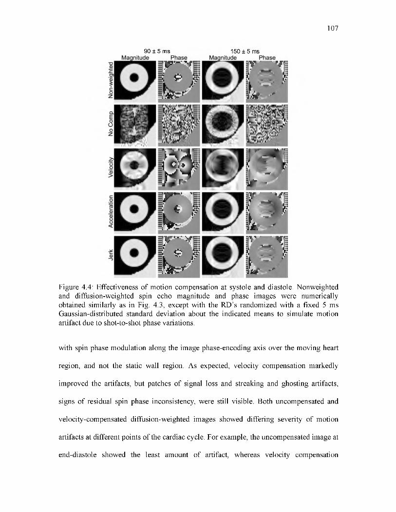
107
90 ± 5 ms 150 ±5 ms
Figure 4.4: Effectiveness of motion compensation at systole and diastole. Nonweighted and diffusion-weighted spin echo magnitude and phase images were numerically obtained similarly as in Fig. 4.3, except with the RD’s randomized with a fixed 5 ms Gaussian-distributed standard deviation about the indicated means to simulate motion artifact due to shot-to-shot phase variations.
with spin phase modulation along the image phase-encoding axis over the moving heart
region, and not the static wall region. As expected, velocity compensation markedly
improved the artifacts, but patches of signal loss and streaking and ghosting artifacts,
signs of residual spin phase inconsistency, were still visible. Both uncompensated and
velocity-compensated diffusion-weighted images showed differing severity of motion
artifacts at different points of the cardiac cycle. For example, the uncompensated image at
end-diastole showed the least amount of artifact, whereas velocity compensation

appeared best at mid-diastole (see Table 4.2), which suggests that different motion terms
likely dominated the motion artifacts at different parts of the cardiac cycle. When
acceleration-compensation was employed, the images obtained appeared nearly identical
to those of the nonweighted images, indicating the effectiveness of motion compensation.
The same applies to the jerk-compensated images, which were not noticeably better than
acceleration-compensated images. The variation of image phase decreased with
increasing motion compensation, with little difference between the acceleration- and jerk-
compensated cases. Again, the RMSE values in Table 4.2 are consistent with these
qualitative observations. The RMSE values of the acceleration- and jerk-compensated
cases are similar to the nonweighted case, which suggests that the novel schemes
sufficiently compensate for motion during diffusion encoding.
Figure 4.5 shows the magnitude images numerically obtained for different motion
compensation schemes at a fixed nominal mean RD (90 ms) but with different levels of
RD variability, for testing the robustness of the schemes to R-R fluctuations. Compared to
the nonweighted images, when a RD standard deviation of 2.0 ms was used, only the
uncompensated image showed significant motion-induced ghosting and streaking
108
Table 4.2. Mean error in the presence of shot-to-shot phase variation.
RD
Scheme
60 ± 5 ms 90 ± 5 ms 120 ± 5 ms 150 ± 5 ms
Nonweighted 0.080 0.020 0.058 0.071No Comp 0.651 0.613 0.633 0.250Velocity 0.299 0.175 0.135 0.374
Acceleration 0.076 0.025 0.073 0.067Jerk 0.080 0.020 0.058 0.071
Entries correspond to the root mean squared error between the numerical phantom magnitude and the simulated image magnitude from various diffusion encoding schemes.

109
90 ± 2 ms Magnitude Phase
90 ± 7.5 ms Magnitude Phase
= ^ -V =i m T ' M
Figure 4.5: Effectiveness of motion compensation and cardiac cycle consistency. Magnitude and phase images were numerically obtained similarly as in Fig. 4.4, except with the same mean readout delay RD of 90 ms (end-systole) and varying degrees of gating consistency, represented by the specified standard deviation of the Gaussian distribution from which the shot-to-shot RD was randomly selected.
artifacts. As the RD standard deviation increased, so did the artifacts seen in the
uncompensated and velocity-compensated cases, albeit in the latter the severity of the
artifacts was visibly reduced. In comparison, acceleration- and jerk-compensated images
showed no visible artifact, even at the largest RD standard deviation (7.5 ms). Similar
patterns were observed in results obtained for other points of the cardiac cycle, or mean
RD values, (not shown). The phase images did not change substantially as the variation in
RD increased. The RMSE values in Table 4.3 support the previous observations, where

110
Table 4.3. Mean error in the presence of shot-to-shot phase variation.
RD
Scheme
90 ± 1 ms 90 ± 2 ms 90 ± 5 ms 90 ± 7.5 ms
Nonweighted 0.004 0.006 0.020 0.023No Comp 0.342 0.546 0.613 0.637Velocity 0.020 0.045 0.175 0.252
Acceleration 0.005 0.007 0.025 0.025Jerk 0.004 0.006 0.020 0.022
Entries correspond to the root mean squared error between the numerical phantom magnitude and the simulated image magnitude from various diffusion encoding schemes.
the error increased when variation in RD increased. Again, the acceleration- and jerk-
compensated cases produced values close to the nonweighted case. Together, the findings
in Figs. 4.3-4.5 and Tables 4.1-4.3 suggest that although velocity-only compensation may
be sufficient when highly reproducible cardiac gating (within 1% of the R-R interval) is
achievable, motion artifacts can be more reliably suppressed by employing higher order
motion compensation.
Figure 4.6 shows representative diffusion-weighted images in three orthogonal
encoding directions obtained with different levels of motion compensation on a live rat.
The non-compensated results showed large patches of signal voids in the entire
myocardium, similar to the effects of intravoxel phase dispersion seen in Fig. 4.3. In
contrast, most of the myocardium was visible in the velocity-compensated images,
although there were still regional areas of signal voids, possibly due to either, or the
combination of, shot-to-shot phase variation (compare to Fig. 4.4) or residual intravoxel
phase dispersion unaccounted by the simplistic motion model. The localized hypointense
patches in the velocity-compensated images did not appear as symmetrical as they do in
the simulation results in Figs. 4.3-4.5, which was likely due to the non-symmetry of the

111
Figure 4.6: Diffusion-weighted images of the heart obtained on a live rat with various degrees of motion compensation. The images are obtained at the same cardiac short-axis location using diffusion encoding in the specified gradient axis and motion compensation scheme.
underlying cardiac kinematics [42]—[44] due to the positioning of the animal. When the
animal is in the prone position, a higher degree of motion is likely to occur in the dorsal
left ventricle away from the chest wall, which could result in more signal loss.
Both acceleration- and jerk-compensation yielded largely artifact-free images of the
entire heart, again similar to Figs. 4.3-4.5. One notable difference between the numerical
and in vivo images was in the jerk-compensated images, where the in vivo images showed
visibly reduced intensity due to the prolonged TE necessary to accommodate the

additional compensating and crusher gradient pulses. This observation was supported by
the quantified SNRs of the in vivo acceleration and jerk-compensated images, which were
14.2, and 6.4, respectively. Consequently, acceleration compensation represented the
optimal tradeoff between motion sensitivity reduction and T2 signal attenuation for
practical imaging.
Finally, Fig. 4.7 shows myofiber helix angle, fractional anisotropy (FA), and mean
diffusivity (MD) maps obtained from DTI using velocity-, acceleration-, and jerk-
112
Helix Angle FA Mean Diffusivity
-90° 0° 90° 0 0.5 1.0 0 1 2 3(x 10-3 mm2/s)
Figure 4.7: DTI images obtained on a live rat using velocity-, acceleration-, and jerk- compensated diffusion encoding in the same cardiac short-axis slice. The helix angle maps obtained from acceleration- and jerk-compensation exhibit the well-known transmural variation from positive to negative helix angles from the endo- to epicardium. However, the maps obtained from jerk-compensation are noisier due to the prolonged TE necessary to accommodate the additional moment nulling gradients. No smoothing was applied to these results.

compensated diffusion-weighted scans on a live rat. The helix angle map obtained from
acceleration-compensated diffusion encoding demonstrates the distinctive rotation from
positive to negative helix angles from the endo- to epicardium [45]. Although the results
need to be validated, to the authors’ knowledge, they are the first demonstrated DTI maps
obtained in live rats. The transmural rotation of the helix angle is also apparent in helix
angle map derived from the jerk-compensated diffusion encoding. However, the lower
SNR associated with the longer TE in the jerk-compensated case results in a noisier helix
angle map and elevated FA, as expected [46]. The transmural rotation in velocity-
compensated case is present in the ventral wall, but not in the dorsal wall where more
motion is suspected. Figure 4.8 shows DTI parameter maps obtained in four more rats
using acceleration compensation. The average MD and FA values over the LV in the
acceleration-compensated case in the 12 rat hearts were found to be 1.44 ± 0.08 x 10"3
mm2/s and 0.41 ± 0.05, respectively, which shows low inter-subject variability. These
measurements are also in general agreement with values previously reported in
Langendorff perfusion studies in the rat (1.01 ± 0.07 x 10"3 mm2/s and 0.34 ± 0.04) [47]
and in vivo studies in the mouse (~1.2 x 10"3 mm2/s and ~0.29) [30], given the dissimilar
experimental setup and species involved.
4.6 Discussion
Results of the motion sensitivity analysis (Figs. 4.3-4.5) reveal that previous attempts
of in vivo diffusion MRI or DTI in the rat heart likely have been complicated by
insufficient motion compensation of the monopolar or bipolar diffusion encoding
gradient waveforms used. Both numerical verification and live animal experimentation
113

114
Helix Angle FA Mean Diffusivity
-90° 0° 90° 0 0.5 1.0 0 1 2 3(x 10'3 mm2/s)
Figure 4.8: Unsmoothed DTI images obtained in four live rats. Again, the helix angle maps exhibit the distinctive counterclockwise transmural rotation of the myocardial fiber orientation. In contrast, fractional anisotropy and mean diffusivity maps show the scalar DTI properties to be relatively homogeneous in the short-axis slice.
demonstrate the feasibility of encoding diffusion while simultaneously reducing the
sensitivity to higher-order motion via the proposed moment-nulled gradient waveforms.
Although waveforms that compensate for progressively higher-order motion are
accompanied by lower achievable b-values and longer TE, acceleration compensation is
shown to provide the necessary and sufficient combination of diffusion encoding, motion
sensitivity reduction, and SNR preservation for practical diffusion MRI. Overall, these

115
findings are highly promising and pave the way for longitudinal evaluation of myocardial
remodeling associated with maturation, disease progression, and recovery in the rat.
The implementation adopted in the current study, by combining gradient pulses of
identical duration but different amplitude in a spin echo setting, is not meant to be
unique. While the principle of motion compensation by gradient moment nulling remains
the same, there exist alternative ways motion-compensated diffusion encoding can be
realized in practice, depending on the specific criteria desired. For example, acceleration-
compensated diffusion encoding can also be carried out by gradient pulses with the same
peak amplitude (either positive or negative polarity) but different durations, as shown in
Fig. 4.9, with the required gradient durations related by,
S2 = 51 (A - x)/(A - 281 + t ) . (4.15)
Under these timing conditions, the gradient waveform can achieve a b-value of
, , o , (T2 - + 2AS2 y - 125f (A + t ) ! b = y ! C ! ( «2 (4 + r) + ------------- +2(^ + 2^ 2- T )! ---------------
5% (A + t )2 {A + 3S2 ) S2t 2 49t 3 (A + 2S 2 - t ) 2 6 + ~60 3
t 2 ( t 2 — At + 2AS2 ) + 3 (A + t ) (2A + S2 + 2r)3{A + 2S2 - t) (416)
The expected main benefit of the implementation using peak-amplitude gradient pulses is
its shorter TE, larger achievable b-value, or both. For instance, utilizing the 400 mT/m
peak-amplitude gradients of the current study, the TE could be shortened by 2.45 ms for
the same b-value of 350 s/mm2. Alternatively, the same 19.43 ms waveform length, T,
would translate to an achievable b-value improvement of 66%, to 580 s/mm2.
Besides different gradient pulse specifications, the proposed diffusion encoding
waveforms with higher-order motion compensation can also be alternatively
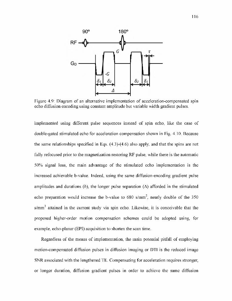
116
90° 180°
Figure 4.9: Diagram of an alternative implementation of acceleration-compensated spin echo diffusion encoding using constant amplitude but variable width gradient pulses.
implemented using different pulse sequences instead of spin echo, like the case of
double-gated stimulated echo for acceleration compensation shown in Fig. 4.10. Because
the same relationships specified in Eqs. (4.3)-(4.6) also apply, and that the spins are not
fully refocused prior to the magnetization restoring RF pulse, while there is the automatic
50% signal loss, the main advantage of the stimulated echo implementation is the
increased achievable b-value. Indeed, using the same diffusion-encoding gradient pulse
amplitudes and durations (6), the longer pulse separation (A) afforded in the stimulated
echo preparation would increase the b-value to 680 s/mm , nearly double of the 350
s/mm2 attained in the current study via spin echo. Likewise, it is conceivable that the
proposed higher-order motion compensation schemes could be adopted using, for
example, echo-planar (EPI) acquisition to shorten the scan time.
Regardless of the means of implementation, the main potential pitfall of employing
motion-compensated diffusion pulses in diffusion imaging or DTI is the reduced image
SNR associated with the lengthened TE. Compensating for acceleration requires stronger,
or longer duration, diffusion gradient pulses in order to achieve the same diffusion

117
ECG
RF
G d
Figure 4.10: Diagram of an alternative implementation of acceleration-compensated, diffusion-weighted gradient pulses in a STEAM sequence for acquisition over two consecutive heartbeats.
weighting b-value when compared to using uncompensated or velocity-compensated
diffusion encoding pulses. This may be problematic when a sufficiently strong gradient
set is unavailable or when imaging tissues with short T2 relaxation. Even though
acceleration-compensation performed the best in the current study, there likely remains a
significant noise contribution in the resulting parameter maps. Advanced recon methods
[48] may be able to both speed acquisition and increase SNR. Finally, strong magnetic
gradient pulses with alternating polarity, like those used here, are more prone to eddy
current effects and concomitant magnetic fields. Phase errors from concomitant fields are
easily eliminated by using a refocusing pulse, similar to the spin echo preparation used in
the present study.
Logistical constraints restricted the current study to a single slice per animal. The
long scan times resulting from the use of multi-shot spin echo acquisition also limited the
study to one DTI set in the majority of the animals. Therefore, intra-subject repeatability
was not directly evaluated. However, good repeatability is implied in the excellent inter-
Jt90° 90°
I
90c

subject reproducibility observed in the tight standard deviations of global DTI
parameters.
Lastly, it should be noted that, while the ability to compensate for higher-order
motion in diffusion MR acquisitions is highly desirable and represents a significant step
of advancement, it is only part of a nuanced approach required to accurately characterize
the myocardial microstructure and fiber orientation via in vivo DTI. For example, tissue
deformation, or strain, is known to skew MR diffusion measurements [49], [50], which
require correcting [23], [27]. The impact on acceleration-compensated diffusion encoding
remains to be investigated, but like the case of bipolar encoding gradient pulses [25],
[26], the partial refocusing of spins that occur during the proposed scheme is expected to
at least partially reduce the errors caused by strain. Another potential physiology-induced
complication that may need to be accounted for are the effects of perfusion on diffusion
measurements [51]. Systematic examinations of these complicating factors are beyond
the scope of the current study, but represent worthy areas of future research.
In conclusion, the present study employed the principles of gradient moment nulling
and derived diffusion-encoding schemes that efficiently compensate for higher motion
components, including acceleration and jerk. The effectiveness of the proposed diffusion-
encoding schemes was evaluated via numerical verification on a realistic motion phantom
of the rat heart, and empirical demonstration of cardiac diffusion MRI on live rats.
Acceleration compensation was found to provide both the necessary and sufficient
compromise among achievable b-value, motion sensitivity reduction, and SNR
preservation for practical diffusion MRI in rats, for the given gradient hardware
capabilities. The resulting sequence was used to demonstrate the first successful DTI
118

myocardial fiber orientation and FA maps obtained in vivo in rats. These findings suggest
that prospective compensation for acceleration, along with lower motion components, can
be an effective alternative or adjunct to high-performance gradient hardware for
improving in vivo cardiac DTI.
4.7 Funding Sources
NIH grants R01 HL092055, S10 RR023017, and R01 NS08376.
4.8 Conflicts of Interest
Christopher Lee Welsh, Edward V.R. DiBella, and Edward W. Hsu declare that they
have no conflicts of interest.
4.9 Statement of Human Studies
No human studies were carried out by the authors for this article.
4.10 Statement of Animal Studies
Animal protocols were approved by the University of Utah Institutional Animal Care
and Use Committee in accordance to the Guide for the Care and Use of Laboratory
Animals issued by the US National Institutes of Health (NIH Publication No. 85-23,
rev.1996).
119

120
[1] W. I. Tseng, J. Dou, T. G. Reese, and V. J. Wedeen, “Imaging myocardial fiberdisarray and intramural strain hypokinesis in hypertrophic cardiomyopathy with MRI,” J. Magn. Reson. Imaging, vol. 23, no. 1, pp. 1-8, Jan. 2006.
[2] M. T. Wu, M. Y. Su, Y. L. Huang, K. R. Chiou, P. Yang, H. B. Pan, T. G. Reese, V.J. Wedeen, and W. I. Tseng, “Sequential changes of myocardial microstructure in patients postmyocardial infarction by diffusion-tensor cardiac MR: correlation with left ventricular structure and function,” Circ. Cardiovasc. Imaging, vol. 2, no. 1, pp. 32-40, Jan. 2009.
[3] N. Toussaint, M. Sermesant, C. T. Stoeck, S. Kozerke, and P. G. Batchelor, “In vivohuman 3D cardiac fibre architecture: reconstruction using curvilinear interpolation of diffusion tensor images,” Med. Image Comput. Comput. Assist. Interv., vol. 13, pp. 418-25, Jan. 2010.
[4] G. Plank, R. A. B. Burton, P. Hales, M. Bishop, T. Mansoori, M. O. Bernabeu, A.Garny, A. J. Prassl, C. Bollensdorff, F. Mason, F. Mahmood, B. Rodriguez, V. Grau, J. E. Schneider, D. Gavaghan, and P. Kohl, “Generation of histo-anatomically representative models of the individual heart: tools and application,” Philos. Trans.A. Math. Phys. Eng. Sci., vol. 367, no. 1896, pp. 2257-92, Jun. 2009.
[5] F. Vadakkumpadan, H. Arevalo, C. Ceritoglu, M. Miller, and N. Trayanova, “Image-based estimation of ventricular fiber orientations for personalized modeling of cardiac electrophysiology,” IEEE Trans. Med. Imaging, vol. 31, no. 5, pp. 1051-60, May 2012.
[6] L. Geerts, P. H. M. Bovendeerd, K. Nicolay, and T. Arts, “Characterization of thenormal cardiac myofiber field in goat measured with MR-diffusion tensor imaging,” Am. J. Physiol. Heart Circ. Physiol., vol. 283, no. 1, pp. H139-45, Jul. 2002.
[7] N. S. Phatak, S. A. Maas, A. I. Veress, N. A. Pack, E. V. R. DiBella, and J. A.Weiss, “Strain measurement in the left ventricle during systole with deformable image registration,” Med. Image Anal., vol. 13, no. 2, pp. 354-61, Apr. 2009.
[8] J. Chen, S. K. Song, W. Liu, M. McLean, J. S. Allen, J. Tan, S. A. Wickline, and X.Yu, “Remodeling of cardiac fiber structure after infarction in rats quantified with diffusion tensor MRI,” Am. J. Physiol. Heart Circ. Physiol., vol. 285, no. 3, pp. H946-54, Sep. 2003.
[9] M. T. Wu, W. I. Tseng, M. Y. Su, C. P. Liu, K. R. Chiou, V. J. Wedeen, T. G.Reese, and C. F. Yang, “Diffusion tensor magnetic resonance imaging mapping the fiber architecture remodeling in human myocardium after infarction: correlation with viability and wall motion,” Circulation, vol. 114, no. 10, pp. 1036-45, Sep. 2006.
4.11 References

121
[10] E. X. Wu, Y. Wu, J. M. Nicholls, J. Wang, S. Liao, S. Zhu, C.-P. P. Lau, and H.-F.F. Tse, “MR diffusion tensor imaging study of postinfarct myocardium structural remodeling in a porcine model,” Magn. Reson. Med., vol. 58, no. 4, pp. 687-95, Oct. 2007.
[11] G. J. Strijkers, A. Bouts, W. M. Blankesteijn, T. H. J. M. Peeters, A. Vilanova, M. C.van Prooijen, H. M. H. F. Sanders, E. Heijman, and K. Nicolay, “Diffusion tensor imaging of left ventricular remodeling in response to myocardial infarction in the mouse,” NMR Biomed., vol. 22, no. 2, pp. 182-90, Feb. 2009.
[12] C. Mekkaoui, S. Huang, G. Dai, T. G. Reese, J. Ruskin, U. Hoffmann, M. P.Jackowski, and D. E. Sosnovik, “Myocardial infarct delineation in vivo using diffusion tensor MRI and the tractographic propagation angle,” J. Cardiovasc. Magn. Reson., vol. 15, no. 1, p. P2, 2013.
[13] P. A. Helm, L. Younes, M. F. Beg, D. B. Ennis, C. Leclercq, O. P. Faris, E.McVeigh, D. Kass, M. I. Miller, and R. L. Winslow, “Evidence of structural remodeling in the dyssynchronous failing heart,” Circ. Res., vol. 98, no. 1, pp. 12532, Jan. 2006.
[14] V. Y. Wang, H. I. Lam, D. B. Ennis, B. R. Cowan, A. A. Young, and M. P. Nash,“Modelling passive diastolic mechanics with quantitative MRI of cardiac structure and function,” Med. Image Anal., vol. 13, no. 5, pp. 773-84, Oct. 2009.
[15] E. W. Hsu, A. L. Muzikant, S. A. Matulevicius, R. C. Penland, and C. S. Henriquez,“Magnetic resonance myocardial fiber-orientation mapping with direct histological correlation,” Am. J. Physiol., vol. 274, no. 5, pp. H1627-34, May 1998.
[16] J. C. Walker, J. M. Guccione, Y. Jiang, P. Zhang, A. W. Wallace, E. W. Hsu, and M.B. Ratcliffe, “Helical myofiber orientation after myocardial infarction and left ventricular surgical restoration in sheep,” J. Thorac. Cardiovasc. Surg., vol. 129, pp. 382-90, Feb. 2005.
[17] Y. Jiang and E. W. Hsu, “Accelerating MR diffusion tensor imaging via filteredreduced-encoding projection-reconstruction,” Magn. Reson. Med., vol. 53, no. 1, pp. 93-102, Jan. 2005.
[18] Y. Wu, L. J. Zhang, C. Zou, H. F. Tse, and E. X. Wu, “Transmural heterogeneity ofleft ventricular myocardium remodeling in postinfarct porcine model revealed by MR diffusion tensor imaging,” J. Magn. Reson. Imaging, vol. 34, no. 1, pp. 43-9, Jul. 2011.
[19] L. Garrido, V. J. Wedeen, K. K. Kwong, U. M. Spencer, and H. L. Kantor,“Anisotropy of water diffusion in the myocardium of the rat,” Circ. Res., vol. 74, no. 5, pp. 789-793, May 1994.
[20] D. F. Scollan, A. Holmes, R. Winslow, and J. Forder, “Histological validation ofmyocardial microstructure obtained from diffusion tensor magnetic resonance
122
imaging,” Am. J. Physiol., vol. 275, no. 6, pp. H2308-18, Dec. 1998.
[21] E. W. Hsu, D. L. Buckley, J. D. Bui, S. J. Blackband, and J. R. Forder, “Two-component diffusion tensor MRI of isolated perfused hearts,” Magn. Reson. Med., vol. 45, no. 6, pp. 1039-45, Jun. 2001.
[22] R. R. Edelman, J. Gaa, V. J. Wedeen, E. Loh, J. M. Hare, P. Prasad, and W. Li, “Invivo measurement of water diffusion in the human heart,” Magn. Reson. Med., vol. 32, no. 3, pp. 423-8, Sep. 1994.
[23] T. G. Reese, R. M. Weisskoff, R. N. Smith, B. R. Rosen, R. E. Dinsmore, and V. J.Wedeen, “Imaging myocardial fiber architecture in vivo with magnetic resonance,” Magn. Reson. Med., vol. 34, no. 6, pp. 786-791, 1995.
[24] W. I. Tseng, T. G. Reese, R. M. Weisskoff, T. J. Brady, and V. J. Wedeen,“Myocardial fiber shortening in humans: initial results of MR imaging,” Radiology, vol. 216, no. 1, pp. 128-39, Jul. 2000.
[25] J. Dou, T. G. Reese, W. I. Tseng, and V. J. Wedeen, “Cardiac diffusion MRI withoutmotion effects,” Magn. Reson. Med., vol. 48, no. 1, pp. 105-14, Jul. 2002.
[26] U. Gamper, P. Boesiger, and S. Kozerke, “Diffusion imaging of the in vivo heartusing spin echoes--considerations on bulk motion sensitivity,” Magn. Reson. Med., vol. 57, no. 2, pp. 331-7, Feb. 2007.
[27] W. I. Tseng, T. G. Reese, R. M. Weisskoff, and V. J. Wedeen, “Cardiac diffusiontensor MRI in vivo without strain correction,” Magn. Reson. Med., vol. 42, pp. 393-403, 1999.
[28] J. Dou, W. I. Tseng, T. G. Reese, and V. J. Wedeen, “Combined diffusion and strainMRI reveals structure and function of human myocardial laminar sheets in vivo,” Magn. Reson. Med., vol. 50, no. 1, pp. 107-13, Jul. 2003.
[29] S. Nielles-Vallespin, C. Mekkaoui, P. Gatehouse, T. G. Reese, J. Keegan, P. F. Ferreira, S. Collins, P. Speier, T. Feiweier, R. de Silva, M. P. Jackowski, D. J. Pennell, D. E. Sosnovik, and D. Firmin, “In vivo diffusion tensor MRI of the human heart: reproducibility of breath-hold and navigator-based approaches,” Magn. Reson. Med., vol. 70, no. 2, pp. 454-464, Sep. 2013.
[30] S. Huang, C. Mekkaoui, H. H. Chen, R. Wang, S. Ngoy, R. Liao, V. J. Wedeen, G. Dai, and D. E. Sosnovik, “Serial diffusion tensor MRI and tractography of the mouse heart in-vivo: impact of ischemia on myocardial microstructure,” J. Cardiovasc. Magn. Reson., vol. 13, no. Suppl 1, p. O28, 2011.
[31] B. Schumacher, P. Pecher, B. U. von Specht, and T. Stegmann, “Induction ofneoangiogenesis in ischemic myocardium by human growth factors: first clinical results of a new treatment of coronary heart disease,” Circulation, vol. 97, no. 7, pp. 645-650, Feb. 1998.
123
[32] F. Ravelli and M. Allessie, “Effects of atrial dilatation on refractory period andvulnerability to atrial fibrillation in the isolated Langendorff-perfused rabbit heart,” Circulation, vol. 96, no. 5, pp. 1686-1695, 1997.
[33] C. Nguyen, Z. Fan, B. Sharif, Y. He, R. Dharmakumar, D. S. Berman, and D. Li, “Invivo three-dimensional high resolution cardiac diffusion-weighted MRI: A motion compensated diffusion-prepared balanced steady-state free precession approach,” Magn. Reson. Med., Nov. 2013.
[34] O. P. Simonetti, R. E. Wendt, and J. L. Duerk, “Significance of the point ofexpansion in interpretation of gradient moments and motion sensitivity,” J. Magn. Reson. Imaging, vol. 1, no. 5, pp. 569-77, 1991.
[35] V. J. Wedeen, R. M. Weisskoff, and B. P. Poncelet, “MRI signal void due to inplane motion is all-or-none,” Magn. Reson. Med., vol. 32, no. 1, pp. 116-20, Jul. 1994.
[36] T. P. Trouard, Y. Sabharwal, M. I. Altbach, and A. F. Gmitro, “Analysis andcomparison of motion-correction techniques in diffusion-weighted imaging,” J. Magn. Reson. Imaging, vol. 6, no. 6, pp. 925-35, 1996.
[37] P. M. Pattany, J. J. Phillips, L. C. Chiu, J. D. Lipcamon, J. L. Duerk, J. M. McNally,and S. N. Mohapatra, “Motion artifact suppression technique (MAST) for MR imaging,” J. Comput. Assist. Tomogr., vol. 11, no. 3, pp. 369-377, 1987.
[38] P. J. Keller and F. W. Wehrli, “Gradient Moment Nulling through the Nth Moment.Application of Binomial Expansion Coefficients to Gradient Amplitudes,” J. Magn. Reson., vol. 78, no. 1, pp. 145-149, 1988.
[39] J. G. Pipe and T. L. Chenevert, “A progressive gradient moment nulling designtechnique,” Magn. Reson. Med., vol. 19, no. 1, pp. 175-9, May 1991.
[40] D. K. Jones, M. A. Horsfield, and A. Simmons, “Optimal strategies for measuringdiffusion in anisotropic systems by magnetic resonance imaging,” Magn. Reson. Med., vol. 42, no. 3, pp. 515-25, Sep. 1999.
[41] Y. Jiang, K. Pandya, O. Smithies, and E. W. Hsu, “Three-dimensional diffusiontensor microscopy of fixed mouse hearts,” Magn. Reson. Med., vol. 52, no. 3, pp. 453-60, Sep. 2004.
[42] E. Oubel, M. De Craene, A. O. Hero, A. Pourmorteza, M. Huguet, G. Avegliano, B.H. Bijnens, and A. F. Frangi, “Cardiac motion estimation by joint alignment of tagged MRI sequences,” Med. Image Anal., vol. 16, no. 1, pp. 339-50, Jan. 2012.
[43] I. Smal, N. Carranza-Herrezuelo, S. Klein, P. Wielopolski, A. Moelker, T.Springeling, M. Bernsen, W. Niessen, and E. Meijering, “Reversible jump MCMC methods for fully automatic motion analysis in tagged MRI,” Med. Image Anal., vol. 16, no. 1, pp. 301-24, Jan. 2012.

124
[44] A. D. Gomez, S. S. Merchant, and E. W. Hsu, “Accurate high-resolutionmeasurements of 3-d tissue dynamics with registration-enhanced displacement encoded MRI,” IEEE Trans. Med. Imaging, vol. 33, no. 6, pp. 1350-62, Jun. 2014.
[45] D. D. Streeter, H. M. Spotnitz, D. P. Patel, J. Ross, and E. H. Sonnenblick, “Fiberorientation in the canine left ventricle during diastole and systole,” Circ. Res., vol. 24, no. 3, pp. 339-47, Mar. 1969.
[46] C. Pierpaoli and P. J. Basser, “Toward a Quantitative Assessment of DiffusionAnisotropy,” Magn. Reson. Med., vol. 36, pp. 893-906, 1996.
[47] P. W. Hales, J. E. Schneider, R. A. B. Burton, B. J. Wright, C. Bollensdorff, and P.Kohl, “Histo-anatomical structure of the living isolated rat heart in two contraction states assessed by diffusion tensor MRI,” Prog. Biophys. Mol. Biol., vol. 110, no. 2-3, pp. 319-30, Oct. 2012.
[48] C. L. Welsh, E. V. R. Dibella, G. Adluru, and E. W. Hsu, “Model-basedreconstruction of undersampled diffusion tensor k-space data,” Magn. Reson. Med., vol. 70, pp. 429-440, Sep. 2013.
[49] S. E. Fischer, M. Stuber, M. B. Scheidegger, and P. Boesiger, “Limitations ofstimulated echo acquisition mode (STEAM) techniques in cardiac applications,” Magn. Reson. Med., vol. 34, no. 1, pp. 80-91, Jul. 1995.
[50] T. G. Reese, V. J. Wedeen, and R. M. Weisskoff, “Measuring Diffusion in thePresence of Material Strain,” J. Magn. Reson. B, vol. 112, no. 3, pp. 253-8, Sep. 1996.
[51] V. Callot, E. Bennett, U. K. M. Decking, R. S. Balaban, and H. Wen, “In vivo studyof microcirculation in canine myocardium using the IVIM method,” Magn. Reson. Med., vol. 50, no. 3, pp. 531-40, Sep. 2003.
CHAPTER 5
EVALUATION OF MYOCARDIAL RESTRUCTURING IN RATS
WITH INDUCED ARTERIAL HYPERTENSION3
5.1 Introduction
The arrangement of myocardial fibers and sheets has important implications on the
mechanical and electrical properties of the heart [1], [2]. For example, the helical
arrangement of cardiac myofibers creates a twisting, or torsional, motion as the heart
contracts, which efficiently ejects blood and reduces stress within the myocardial walls
[3]. Another study has shown that branching structures within cardiac tissue can produce
slow conduction of electrical signals [4]. Cardiac pathologies have been shown to affect
cardiac microstructure, which in turn affects the overall function of the heart [5], [6].
Being able to accurately characterize cardiac microstructure can be used to quantify
damage due to pathology and tissue remodeling during treatment. In addition, cardiac
microstructural information has been used to create accurate mechanical [7]-[9] and
electrical [10]-[12] models of the heart in order to simulate pathology [13]-[15],
treatment [16], or changes in cardiac mechanics due to microstructural changes [17]-
[19].
3 Included with permission by Christopher L. Welsh, Edward V.R. DiBella, Arnold David Gomez, Yufeng Huang, and Edward W. Hsu from a manuscript in preparation entitled “Evaluation of Myocardial Restructuring in Rats with Induced Arterial Hypertension.”
Diffusion tensor imaging (DTI) [20] has emerged as the preferred noninvasive, or
nondestructive, technique for characterizing the microstructure of tissues including the
myocardium. The primary direction of diffusion, as derived from DTI, has been shown to
correlate well with the primary myofiber orientation in cardiac tissue [21]. Other DTI
parameters, such as the tertiary eigenvector, correlate to the direction normal to the
myocardial sheet structures and have been used to quantify the distribution of sheet
orientations in cardiac tissue [22], [23]. Scalar values that characterize the arrangement of
tissue microstructure can be derived from the diffusion tensor as well. The most common
of these are fractional anisotropy (FA) and mean diffusivity (MD). The FA is the degree
of anisotropic diffusion and is a measure of how organized biological tissue is. The MD
has been related to the properties of the extracellular space within biological tissue, where
an increase in extracellular space generally corresponds to an increase in measured MD.
Diffusion tensor imaging has been used to quantify the effects of different pathologies
on cardiac microstructure by demonstrating variation in certain DTI parameters. For
example, cardiac DTI studies have shown that FA decreases and MD increases in the
presence of cardiac fibrosis [24]. Similarly, other studies have shown myofiber disarray
in areas of myocardial infarction (MI) [25], [26]. Furthermore, DTI has been used to
study hypertrophic cardiac myopathy (HCM) in conjunction with strain imaging. Hearts
with HCM, in addition to hypokinesis, displayed an increase in fiber disarray, reflected
by reduced FA [5]. More recently, studies have reported conflicting results with regards
to changes in the orientation of sheet structures, or sheetlets, in the presence of pathology.
Some have reported that the distributions of sheet angles become more similar in systole
and diastole in the presence of HCM [27]. Others believe that these findings are affected
126

by strain when measuring diffusion in vivo [28], [29]. Further study, including
histological validation and additional experiments with in vivo cardiac DTI, is needed to
resolve these conflicting findings.
The majority of cardiac DTI studies have been performed ex vivo [30]-[32] or in vitro
[33]-[35] due to the complications of implementing diffusion encoding in the beating
heart. In vivo cardiac DTI has been previously demonstrated [36]-[38] but has seen more
widespread usage in recent years [39]-[41] thanks to motion-compensating techniques,
which include using STEAM diffusion encoding with navigators [42] and velocity-
compensated bipolar diffusion pulses in a spin echo preparation [43]. In vivo cardiac DTI
has been demonstrated in humans and mice using these methods. However, in vivo
cardiac DTI in rats, another important animal for cardiac modeling, was only just recently
shown to be feasible using a novel acceleration-compensated diffusion-encoding scheme
[44]. This study showed that cardiac motion, with higher-order components up to
acceleration, needs to be compensated for in order to reduce signal loss. This allowed for
the first DTI measurements in the living rat heart and opened the door to performing
longitudinal studies in the rat heart for the first time. However, since the acceleration-
compensated DTI approach employs a spin echo preparation, where only one line of k-
space is acquired per breath, the approach requires long scan times. Scan time could be
reduced using model-based reconstruction, where the diffusion tensor is reconstructed
directly from the undersampled k-space [45]. Previous work has shown that the model-
based reconstruction approach is able to estimate diffusion tensors accurately from fewer
MRI measurements.
In this study, in vivo cardiac DTI was used to study changes in the cardiac
127

microstructure in an experimental rat model of heart disease over time. Transgenic rats,
which overexpress the hormone prorenin when exposed to a gene activator, were scanned
prior to and two weeks postinduction using acceleration-compensated DTI. These
transgenic rats are known to develop arterial hypertension after induction [46]. The goal
of this study is to characterize the time course of microstructural changes and to assess
the degree of changes in the heart due to increased after load. Previous studies in the
prorenin rat model have shown that there are detectable changes in the cardiac tissue four
weeks postinduction using histology. Here, in vivo cardiac DTI is evaluated to determine
whether it is sensitive to these microstructural changes at an earlier time point, with the
added benefit of being noninvasive and nondestructive. The types of microstructural
changes, including changes in cell morphology and myofiber arrangement, will also be
determined from the DTI results. The application of model-based compressed sensing
reconstruction to undersampled DTI data will also be evaluated to determine the
feasibility of reducing scan time without sacrificing accuracy or sensitivity to
microstructural changes over time.
5.2 Methods
5.2.1 Animal Model
In order to study the effects of plasma prorenin on arterial blood pressure, a
transgenic, inducible, Wistar Kyoto (WKY) rat model that overexpresses hepatic prorenin
was previously generated [46]. by incorporating rat prorenin under the cytochrome
p4501a1 promoter. Overexpression of prorenin was induced by administering 0.3% of the
gene activator indole-3-carbinol (I3C) to the rats. In the current study, transgenic (n = 6)
128

and wild type (n =3) rats (male, 310 g average weight, 4.5 months average age) were
studied using protocols approved by the University of Utah Institutional Animal Care and
Use Committee in accordance to the Guide for the Care and Use of Laboratory Animals
issued by the US National Institutes of Health (NIH Publication No. 85-23, rev. 1996).
Scanning sessions were performed one day prior to and approximately two weeks (13.6
+/- 0.5 days) after I3C induction in both groups. To prepare for imaging, the animals
were anesthetized using 3.5% isoflurane in pure O2 (3.0 L/min). The animal’s vital signs,
including heart and respiratory rate, blood oxygenation level, and rectal temperature,
were continuously monitored and used to adjust the level of anesthesia when needed.
5.2.2 In Vivo Imaging in Rats
All MR imaging was performed on a Bruker Biospec 70/30 instrument (Bruker
Biospin, Billerica, MA) equipped with a 600 mT/m gradient set (BGA-12S) and a 72 mm
volume coil. In order to quantify cardiac morphology and global function, high
resolution, retrospectively-gated FLASH-CINE images (48 ms TR, 2.4 ms TE, 392 x 392
matrix size, 0.11 x 0.11 x 1.5 mm3 voxel size, 4.48 x 4.48 cm2 FOV, 100 signal
repetitions, 350 s/mm2 b-value, 5 slices, 15 frames) in the short-axis were acquired in
each rat. In addition, a single slice was acquired in the four chamber, long-axis view
using the same acquisition parameters as the short-axis scans.
Cardiac DTI was performed using acceleration-compensated diffusion encoding to
compensate for the beating motion of the heart in the live rats. Similar to previous work,
the acceleration-compensated diffusion encoding was incorporated into a spin-echo pulse
sequence to obtain diffusion-weighted images (1000 ms TR, 128 x 128 matrix size, 0.35
129
x 0.35 x 3.0 mm3 voxel size, 4.48 x 4.48 cm2 FOV, 1 signal average, 350 s/mm2 b-value,
1 short-axis slice) encoded in an optimized set of 24 directions at end-systole and in an
optimized set of 12 directions at end-diastole, along with one nonweighted reference (b0)
image at each cardiac phase. Dual cardiac and respiratory gating were employed to
acquire DWIs at the desired cardiac phase. Differing numbers of diffusion encoding
directions were acquired at systole and diastole because of practical considerations in
scan time and in-plane resolution. The total required scan time was approximately 120
minutes for each subject. It was found that the quality of diffusion imaging was not
sufficient for DTI calculation at diastole for all animals. In the end, DTI data with
sufficient quality were obtained at baseline and two weeks postinduction in three
transgenic rats and three wild type rats
5.2.3 Image Processing and Statistics
5.2.3.1 Quantification o f Cardiac Structure and Function
Measures of cardiac morphology were derived from the FLASH-CINE images
described in section 5.2.2. Left ventricular wall thickness and diameter (inner and outer)
were measured at end-systole and end-diastole. Mean values for each were derived from
repeated measurements performed in Amira (FEI Life Sciences, OR, USA). Wall
thickness measurements were made at a mid-ventricular short-axis slice, with
measurements spread evenly around the left ventricle, along with ventricular diameters
measured in the same slice.
Basic measures of the global heart function were determined by calculating the left
ventricular volume at systole and diastole, from which stroke volume and ejection
130

fraction could be determined. The LV volume was estimated by segmenting the
ventricular cavity in five short-axis slices that covered the left ventricle. Image
segmentation was performed manually in Amira. The total number of pixels within the
LV were then summed and multiplied by the in-plane resolution and slice thickness in
order to estimate the ventricular volume.
Using the estimated volumes at systole and diastole, stroke volume could be
calculated as
SV = EDV - ESV, (5.1)
where EDV is the end-diastolic volume and ESV is the end-systolic volume. Similarly,
the ejection fraction can be can be calculated as
BFl%) = 10„ x J L (5.2)
Diffusion tensor calculation was performed using a constrained linear least squares
(CLLS) approach with Cholesky parameterization [47] to ensure the symmetric positive
definiteness (SPD) property of the resulting tensors. Fractional anisotropy (FA) and mean
diffusivity (MD) maps were generated from the resulting diffusion tensors via traditional
methods and mean values were calculated within the left ventricular myocardium of each
subject for each scanning session for longitudinal comparison.
Helix angle maps were obtained within the myocardium at end-systole by projecting
the primary eigenvector onto the tangential plane of the myocardium and then measuring
the inclination from the circumferential plane. The variation of the helix angle across the
myocardium was then quantified by plotting the helix angle at each pixel versus its
transmural position. A straight line was fitted to the resulting scatter plot using a robust
131

nonlinear regression analysis [48]. The slope of the line from the robust fit provided a
measure of the variation in helix angle across the myocardium. The robust standard
deviation of the residuals (RSDR) [48] between the measured helix angle values and the
fitted line was computed to evaluate the “goodness of fit” in each rat.
In order to measure the myocardial sheet structure, structural information was defined
with respect to a local coordinate system constructed using distribution of potentials
approach, known as the Laplace Dirichlet method for structural definition briefly
described as follows [49]. After segmentation of the left ventricle, a pixel-wise finite-
element mesh was constructed using hexahedral elements and assigned a potential of one
at the endocardium and zero at the epicardium (Dirichlet boundary conditions). The
Laplace equation was solved to obtain pixel potentials whose spatial gradients constitute
local radial directions from which circumferential directions were obtained assuming a
primary longitudinal direction normal to the slices via cross product. Instead of the rule-
based method described in [49], structural information was directly calculated from the
eigenvectors of the diffusion tensor at every voxel per DT-MRI results. From previous
observations that associate sheet structures to principal diffusivity directions [50], [51],
voxel-wise sheet angles were defined as the angles of elevation of the third eigenvector
with respect to the radial-tangential plane (i.e., the plane normal to the local longitudinal
direction) [28]. The distribution of the sheet angle was further quantified by fitting a
quadratic polynomial to the sheet angle histogram. The coefficient of the second order
term in the quadratic polynomial provided a measure of the concavity of the histogram.
132

5.2.3.2 Statistical Analysis
In order to determine significant changes in the quantitative measurements described
in section 5.2.3.1, a paired t-test was applied to each case. The mean measurement for
each DTI, cardiac morphology, and cardiac function parameter was compared at baseline
(prior to induction) and approximately two weeks after induction for the transgenic and
wild type populations. A student’s t-test was applied to determine whether there was a
significant change in the measurements between the two time points, where significance
was determined by a P-value less than 0.05.
5.2.4 Comparison of Reconstruction Methods for Undersampled DTI Data
Because the acceleration-compensated diffusion encoding was incorporated into a
spin echo preparation, where one line of k-space was acquired per breath, the resulting
scan times were somewhat prohibitive. The total acquisition time could be reduced by
acquiring fewer measurements in k-space, encoding fewer diffusion directions, or a
combination of both. Model-based compressed sensing has been shown to accurately
reconstruct DTI data from fewer diffusion measurements [45]. In this study, model-based
reconstruction was implemented on retrospectively undersampled DTI acquired in this
study in order to assess the feasibility of preserving the accuracy of the DTI solution
when acquiring fewer measurements in k-space and diffusion encodings, allowing for
shorter scan times or the acquisition of multiple slices. For this study, the model-based
reconstruction technique that was presented previously was used with minor
modifications, to improve its overall performance. Changes to the implementation
included setting the image phase estimate in the signal model equal to the phase map
133
estimated from compressed sensing reconstruction of complex diffusion weighted images
using spatial and temporal regularization (CS-STCR, see more details in the following
paragraph). In addition, the derived diffusion tensor solution from the CS-STCR scheme
was used to initialize the diffusion tensor estimate in the model-based reconstruction,
ensuring that the solution converged to the global minimum instead of a local minimum.
Reduced acquisition time was simulated by retrospectively undersampling the acquired k-
space by a factor of two (R = 2) and using half of the diffusion encoding directions (a
subset of 12 optimized directions) resulting in an overall scan time reduction of four. The
DTI parameters calculated in 5.3.3.1 were also derived from the model-based
reconstruction results in order to determine whether the approach preserves the sensitivity
to microstructural changes over time, which were observed in fully-sampled acquisitions
that are reconstructed traditionally.
The performance of model-based reconstruction was compared against two other
forms of traditional compressed sensing. (Note that prior-based, constrained
reconstruction is implied when discussing “compressed sensing”). The first scheme was
compressed sensing with a spatial total variation (TV) constraint (CS-TV), which is one
of the simplest form of compressed sensing reconstruction [52]. The second comparison
scheme was the previously mentioned compressed sensing with spatial and temporal total
variation regularization (CS-STCR) [53], [54]. Here, in addition to a spatial total
variation constraint, a total variation constraint was applied in the diffusion-encoding
dimension. Since the magnitude within a given pixel is not expected to vary smoothly
from one diffusion-encoding direction to the next, reordering was performed on a pixel-
by-pixel basis. The reordering of each pixel, from lowest to highest, was accomplished
134

using a low-resolution prior derived from the fully-sampled low frequency portion of k-
space [55]. Smoothness across diffusion encoding directions was enforced using total
variation applied to the reordered pixels. The same degree of scan time reduction that was
simulated for the model-based reconstruction was applied to the CS-TV and CS-STCR
reconstructions as well.
Diffusion tensors were derived from the diffusion-weighted images that were
reconstructed using the CS-TV and CS-STCR schemes using traditional methods. Mean
FA, mean MD, and transmural variation of helix angle were derived from the resulting
diffusion tensors, similar to the procedure described in Section 5.2.3.1, and were
compared to the same measurements derived from model-based reconstruction and from
fully-sampled data in order to assess the accuracy of the alternative reconstruction
schemes.
5.3 Results
5.3.1 Cardiac morphology and Function
Results of the cardiac morphology analysis in systole and diastole are shown in Figs.
5.1 and 5.2. The cardiac morphology was consistent at baseline and week 2 in the wild
type rat at both phases of the cardiac cycle with no apparent qualitative differences
between baseline and week 2 scans. However, the cardiac morphology of the transgenic
rat appears to change significantly from baseline to week 2. In both systole and diastole,
the inner and outer diameters of the left ventricle appear to decrease. The bar graphs in
Fig. 5.2 confirm these qualitative observations, indicating there was a significant decrease
in the inner diameter of the left ventricle in the transgenic group. However, Fig. 5.2 also
135
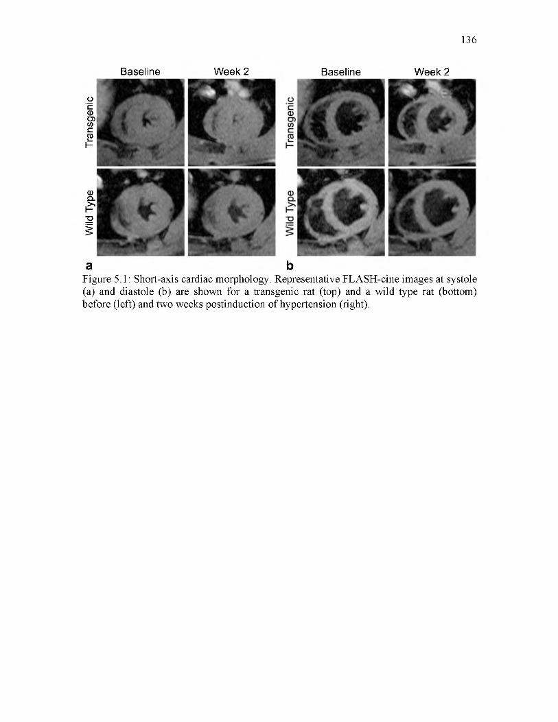
Wild
Ty
pe
Tran
sgen
ic
136
Baseline
a
Week 2 Baseline Week 2
bFigure 5.1: Short-axis cardiac morphology. Representative FLASH-cine images at systole(a) and diastole (b) are shown for a transgenic rat (top) and a wild type rat (bottom) before (left) and two weeks postinduction of hypertension (right).

137
LV Inner Diameter, Systole
Baseline Week 2
E 4'
cd d) 2'CO
Wall Thickness, SystoleBaseline Week 2
✓<5*
Baseline ■ Week 2
LV Inner Diameter, Diastole
E »
CD 0 E cob 2'
cP>
E E,w w CD C.9 2H
= 1' CO
Wall Thickness, DiastoleBaseline Week 2
L Xsp
✓Figure 5.2: Measurements of cardiac morphology. Bar graphs at systole (a) and diastole(b) show the group means and standard error of the means of the LV inner diameter (top) and wall thickness (bottom) before and two weeks postinduction of hypertension. A significant decrease in the inner diameter of the LV from baseline to week 2 was observed in the transgenic group in systole and diastole. No significant change in wall thickness at systole or diastole occurred in either group.
shows that there was not a significant change in wall thickness in either group at systole
or diastole. The preserved wall thickness implies that there was a corresponding decrease
in the outer diameter of the LV in addition to the decrease in inner diameter. Figures 5.1
and 5.2 demonstrate a significant change in the cardiac morphology, which was likely
due to the induced hypertension. Microstructural changes likely accompany the observed
macroscopic changes in the myocardium.

Figure 5.3 shows the results of the cardiac functional analysis. The decrease in the
inner diameter of the left ventricle at systole and diastole, as seen in Fig. 5.2,
corresponded to a significant decrease in LV volume at both phases of the cardiac cycle
in the transgenic group at week 2 compared to baseline. In addition to the decrease in
ventricular volume, the stroke volume also decreased in the transgenic group. However,
the ejection fraction remained constant in both animal groups at both time points even in
138
40-i
o 20-
o 10-
LV Volume, SystoleBaseline Week 2
A'
LV Stroke VolumeBaseline Week 2
cu
cooro
oCDi l l
250-I
200 -
150-
LV Volume, Diastole
Baseline Week 2
100-
100-
LV Ejection FractionBaseline Week 2
Figure 5.3: Analysis of cardiac function. Bar graphs representing the group means of LV volume at systole (a) and diastole (b) are shown along with the group mean averages of LV stroke volume (c) and ejection fraction (d) in the transgenic and wild type groups. A significant decrease in LV volume was observed in the transgenic rats at systole and diastole. In addition, a corresponding decrease in stroke volume from baseline to week 2 was observed in the transgenic group. No significant change in ejection fraction occurred in either group.

139
the presence of induced hypertension. The ejection fraction did not change because of the
decrease in heart size that resulted in lower stroke and end-diastolic volumes, both of
which are involved in determining ejection fraction (see Eq. (5.2)). The induced
hypertension in the transgenic rats appears to have affected diastolic filling and cardiac
output, both of which are important indicators of cardiac function.
5.3.2 DTI Results
Figure 5.4 shows representative fractional anisotropy (FA) maps from the transgenic
and wild type groups. There are not many appreciable differences in the FA maps from
baseline to week 2 in either group. On the whole, the FA maps generated from the two
groups appear mostly homogenous. Regions of increased FA are present in both groups,
Baseline Week 2
A'
Baseline W eek 2
✓
0 0.7Figure 5.4: End-systole fractional anisotropy. Representative false color coded maps (a) are shown for a transgenic rat (top) and a wild type rat (bottom) before (left) and two weeks postinduction of hypertension (right). The bar graph (b) shows the group means and standard error of the means. No significant change between the two time points was observed in either group.

140
but they are most likely a result of noise in the acquired diffusion signal. The comparison
of FA group means confirm that there was not a significant change in FA in either group
from baseline to week 2 .
Mean diffusivity maps acquired in systole are shown in Fig. 5.5. Similar to the FA
maps, the MD maps generated from both groups of rats do not demonstrate obvious
differences. The MD values throughout the myocardium are fairly homogeneous at both
time points, with some areas of increased MD near the endocardium that are likely due to
blood perfusion. The comparison of group means in Fig. 5.5(b) indicates there was not a
significant difference in MD values from baseline to week 2 in either group of rat similar
to the results seen in FA maps. Together, the results in Figs. 5.4-5.5 indicate that there
was no detectable change in FA and MD, both of which are traditional measures of
microstructural changes in cardiac pathology, in the transgenic rats two weeks after
Baseline W eek 2
o"cCDO)(/)c03
<1)Cl
£
I
a b0 2.5
Figure 5.5: End-systole mean diffusivity. Representative false color coded maps (a) are shown for a transgenic rat (top) and a wild type rat (bottom) before (left) and two weeks postinduction of hypertension (right). The bar graph (b) shows the group means and standard error of the means. No significant change between the two time points was observed in either group.
Baseline Week 2

induction of hypertension.
Figure 5.6 compares helix angle maps from DTI data acquired in both groups of rats.
The characteristic transmural variation of the helix angle, from positive to negative
angles, when moving from endo- to epicardium is prominent in the maps obtained in both
transgenic and wild type rats. The helix angle maps from the wild type rat acquired at
baseline and week 2 are quite similar to each other. However, the helix angle maps from
the transgenic rat acquired at the two time points are not as consistent. There is a wider
range of angles in the helix angle map from the week 2 scan, with more negative angles
than the baseline case. The presence of a wider range of helix angles indicates an increase
in transmural variation of the helix angle across the myocardium, resulting in more
141
Baseline Week 2
c 200-oCD 150-CD
> ^— ."CD
COCD 100-
L - "O
E 50-COcCD
h - 0-
Baseline W eek 2
Figure 5.6: End-systole fiber helix angle. Representative false color coded maps (a) are shown for a transgenic rat (top) and a wild type rat (bottom) before (left) and two weeks postinduction of hypertension (right). The bar graph (b) shows the group means of the transmural variation of helix angle. A significant increase in transmural variation from baseline to week 2 was observed in the transgenic group, while there was no significant change between the two time points in the wild type group.

myocardial fibers that are aligned in the long axis (angles near ± 90°). These results are
confirmed by the group mean analysis in Fig. 5.6(b). A significant increase in the
transmural variation of the helix angle was observed in the transgenic group, confirming
the qualitative observations, while there was not a similar increase in the wild type group.
The steepening of the helix angle has been proposed as a compensatory mechanism for
increased after load caused by systemic hypertension [56], which would be expected in
the transgenic population in this study. The mean RSDR values at both time points in the
wild type (27.59 ± 1.81°) and transgenic (24.24 ± 2.32°) groups were not significantly
different, indicating a similar “goodness of fit” in both groups. The results in Fig. 5.6
suggest that there were changes in the myocardial microstructure that were more apparent
in the fiber orientation measurements than in the FA and MD measurements at two weeks
postinduction.
Histograms representing the distribution of sheet angles in representative transgenic
and wild type rats are shown in Fig. 5.7. The sheet angle distributions generated from the
wild type rat appear more similar at baseline and week 2 than the corresponding
distributions obtained from the transgenic rat. The concavity of the sheet angle
distributions increased, or became less concave-down, in both groups at week 2, but the
change in concavity was significant only in the transgenic group. The changes in helix
angle maps and sheet angle distributions, as seen in Figs. 5.6 and 5.7, suggest that there
were microstructural changes in the fiber and sheet structure of the myocardium that were
observable as early as two weeks after induction in the transgenic rats. In addition these
results indicate that helix and sheet angle measurements may be more sensitive to
microstructural changes due to hypertension than more traditional measures, such as FA
142

143
Baseline Week 2
>% 5.0x1 O S+J>03 O Co O
Baseline Week 2
— I-5.0x1 O'6-
-1.0x1 O'5-
ETO i_O) -1.0*10‘5,0 -t—*
1
I T
-1.5x1 O’5-1
Sheet Angle (deg) Sheet Angle (deg)
Figure 5.7: End-systole sheet angle. Representative sheet angle histograms (a) are shown for a transgenic rat (top) and a wild type rat (bottom) before (left) and two weeks postinduction of hypertension (right). The bar graph (b) shows the group means and standard error of the means of the concavity of the sheet angle distributions. There is a significant increase in the concavity of the sheet angle distribution in the transgenic group from baseline to week 2, while no significant change between the two time points was observed in the wild type group.
and MD.
5.3.3 Comparison of Reconstruction Methods
Figure 5.8 compares the FA maps derived from retrospectively undersampled DTI
data reconstructed from the schemes detailed in Section 5.2.4. The FA map reconstructed
from CS-TV data appears less homogeneous than the other maps, with several areas of
elevated FA, which are most likely due to artifact instead of an anomaly in the
myocardial tissue. The FA maps generated from CS-STCR and MB appear similar to
each other, but both contain FA values lower than the fully sampled case. The group
mean analysis, as seen in Fig. 5.8(b), indicates that all reconstruction methods produce
constant FA values from baseline to week 2 in both groups of rats, similar to the results in
Fig. 5.4. However, the alternative reconstruction methods produce FA values that are

144
CS-TV CS-STCR MB FullAcq
Figure 5.8: Reduced scan time fractional anisotropy. Representative false color coded maps (a) are shown for a transgenic rat that were reconstructed via compressed sensing with a spatial total variation constraint (CS-TV), compressed sensing with a spatial and temporal TV constraint (CS-STCR), model-based reconstruction (MB), and traditional reconstruction with fully sampled data (Full Acq). The bar graph (b) shows the group means and standard error of the means resulting from each reconstruction scheme. No significant change between the two time points was observed in either group or from any of the reconstruction schemes.
lower at week 2 compared to baseline, but the FA values were not significantly lower
according to the applied statistical test. Overall, the alternative reconstruction methods
slightly underestimate FA compared to the fully sampled case. The lower FA values
could be a result of the image smoothing inherent to the reconstruction methods
employed in this study. Previous studies have shown that smoothing can produce lower
FA values [57], [58].
MD maps derived from the alternative reconstruction schemes are shown in Fig. 5.9,

145
CS-TV CS-STCR MB FullAcq
Figure 5.9: Reduced scan time mean diffusivity. Representative false color coded maps (a) are shown for a transgenic rat that were reconstructed via compressed sensing with a spatial total variation constraint (CS-TV), compressed sensing with a spatial and temporal TV constraint (CS-STCR), model-based reconstruction (MB), and traditional reconstruction with fully sampled data (Full Acq). The bar graph (b) shows the group means and standard error of the means resulting from each reconstruction scheme. No significant change between the two time points was observed in either group or from any of the reconstruction schemes.
all of which appear highly similar to the MD map generated from the full acquisition.
Regions with increased MD along the endocardium were present in all cases. No apparent
under- or overestimation of MD was present in any of the maps compared to the full
acquisition case. The group mean analysis in Fig. 5.9(b) confirms the qualitative
observations, with little difference in the average MD values between the reconstruction
schemes and the fully sampled case in both groups of rats.
Figure 5.10 compares the helix angle maps generated from each of the reconstruction

146
CS-TV CS-STCR MB FullAcq
Figure 5.10: Reduced scan time fiber helix angle. Representative false color coded maps (a) are shown for a transgenic rat that were reconstructed via compressed sensing with a spatial total variation constraint (CS-TV), compressed sensing with a spatial and temporal TV constraint (CS-STCR), model-based reconstruction (MB), and traditional reconstruction with fully sampled data (Full Acq). The bar graph (b) shows the group means and standard error of the means resulting from each reconstruction scheme. A significant increase in transmural variation of the helix angle was observed in the transgenic group in each of the reconstruction schemes.
schemes in a representative transgenic rat. The helix angle map generated from CS-TV
appears to be the most dissimilar to the fully sampled helix angle map, while the helix
angle map reconstructed from the MB method appears the most similar, preserving the
transmural variation of helix angle the best out of all of the alternative reconstruction
schemes tested. The increase in transmural variation of the helix angle from baseline to
week 2 in the transgenic group (previously seen in Fig. 5.6) was preserved in each of the
reconstruction schemes, as seen in group mean analysis in Fig. 5.10(b). Additionally,
there is no significant change in the transmural variation from baseline to week 2 in the

wild type group in any of the reconstruction schemes. Therefore, all of the reconstruction
schemes preserved the sensitivity to changes in the fiber structure that were detected in
the full acquisition.
The performance of the different reconstruction schemes in estimating myocardial
sheet angle is shown in Fig. 5.11. The sheet angle distributions generated from the CS-
STCR and MB reconstruction schemes are similar to each other, but appear different to
147
Baseline— CS-TV
W eek 2
1x10 - S
>CD OO -1x10'6-OE -2x10‘6- c o
O 5 -3x10‘6-lC/5
X -4x1 O'6-
Sheet Angle (deg)
Transgenic
Baseline W eek 2
m r
— CS-TV
Sheet Angle (deg)
Wild Type
1x1 of
o-1x1 O'6,
E -2x1 O'6' CDI—O) eO -3*1 O'6-
-4—»C/)X -4x1 O'6,
Baseline W eek 2
" I I I -
T
/Figure 5.11: Reduced scan time sheet angle. Representative sheet angle distriubtions (a) are shown for a transgenic rat that were reconstructed via compressed sensing with a spatial total variation constraint (CS-TV), compressed sensing with a spatial and temporal TV constraint (CS-STCR), model-based reconstruction (MB), and traditional reconstruction with fully sampled data (Full Acq). The bar graph (b) shows the group means and standard error of the means resulting from each reconstruction scheme. An increase in the concavity of the sheet angle distributions was observed in the transgenic case in each of the reconstruction schemes, but the increase was only considered significant in the full acquisition case.

the distributions generated from the CS-TV reconstruction and from the full acquisition.
Similar to Fig. 5.7, an increase in the concavity of the sheet angle distribution, or
becoming less concave down, from baseline to week 2 was observed in all of the
reconstruction schemes in the transgenic group, but the increase in concavity was not
significant in the alternative reconstruction schemes tested here. The results in Fig.
5.11(b) indicate that the reconstruction schemes do not preserve the sensitivity to changes
in the sheet structure observed in the full acquisition, in particular, the change in
concavity of the sheet angle distributions in systole. The reduced sensitivity to changes in
sheet structure may come from the smoothing inherent to the reconstruction methods that
were evaluated.
5.4 Discussion
Results from the group mean analysis of DTI parameters reveal that in vivo DTI was
able to detect myocardial structural remodeling, in the form of an increase in the
transmural variation of the fiber helix angle (see Fig. 5.6), at two weeks postinduction of
arterial hypertension in the transgenic rats, earlier than at four weeks in a previous study
[46]. Additionally, there were also observable changes in the sheet structure (see Fig.
5.7). The earlier detection of pathological structural alterations can be directly attributed
to the use of repeated measurement statistics made possible by employing in vivo DTI in
the study protocol. Without the technique, different animals would need to be used at
different time points. As demonstration of the latter case, unpaired t-test of the group
means of transmural helix angle rotation between the two animal groups at each pre
induction and 2-week time points would have returned insignificant differences.
148
The results also suggest that, in terms of DTI parameters for detecting myocardial
microstructural changes, measures of structural orientations appear to be more sensitive
than scalar quantities of FA and MD (see Figs. 5.4 and 5.5). The study would have
reached different conclusions if changes in only FA and MD were examined. On the
surface, the unchanged FA and MD are in contrast to previous cardiac pathology studies.
A possible explanation for this discrepancy is that arterial hypertension actually causes
different forms of myocardial remodeling, including at least hypertrophy (specifically
enlargement of myocytes) and fibrosis. Myocardial fibrosis has been shown to result in
decreased FA and increased MD [24]. However, hypertrophy as seen in hypertrophic
cardiomyopathy (HCM) has been shown to decrease MD as the extracellular space
becomes smaller as myocytes become larger. Therefore, the effects of cardiac fibrosis and
HCM, both of which are likely to be present in early stage remodeling from arterial
hypertension, could offset each other in their effects on FA and MD, resulting in
unchanged DTI scalar parameter in the transgenic group.
The functional consequences of the observed microstructural changes (as seen in the
DTI results in Section 5.3.2) can be interpreted in light of the cardiac morphology and
global metrics (from CINE imagery in Section 5.3.1). It is not surprising to observe an
increase of helical angle slope (see Fig. 5.6) associated with hypertension. Slope
increments are a manifestation of preferential remodeling in the longitudinal direction,
which has also been observed as a compensatory response to chronic hypertension
consisting of myocytes and perimysial collagen longitudinal alignment [56]. However,
left-ventricular ejection fraction remains unchanged (see Fig. 5.3) despite firm evidence
of aortic hypertension, suggesting that this metric offers little in terms of monitoring the
149

state of the failing heart in this animal model, since, under increased afterload it is
possible to preserve, or even increase, hemodynamic work output despite a reduced
stroke volume compared to a healthy heart. It is worth noting that a large portion of
cardiac failure in humans occurs in individuals with preserved ejection fraction, and that
strain and strain-sensitive microstructural observations, such as in vivo DT-MRI
presented here have been suggested as better alternatives for disease progression
monitoring [29], [59]-[61].
Changes in the sheet angle distribution were observed in some of the transgenic rats
in DTI data that were acquired in diastole (n = 3). The sheet angle distributions from two
transgenic rats, in systole and diastole, are shown in Fig. 5.12. In contrast to healthy
myocardial tissue, where a clear change in concavity of the sheet angle distribution is
observed as sheet angle populations reconfigure from diastole to systole [61], the
150
Baseline W eek 2
Figure 5.12: End-systole and end-diastole sheet angle. Sheet angle histograms from two transgenic rats are shown at systole (blue) and diastole (red) before (left) and two weeks postinduction of hypertension (right). In general, the systolic and diastolic sheet angle distributions are more similar at week 2 than at the baseline scan for the two rats shown here.

observed trend in lack of sheet angle distribution changes in the transgenic rats at week
two are consistent with diastolic deficiency expected in hypertensive hypertrophic
cardiomyopathy; myocardial hypertrophy and diffused fibrosis often result in tissue
stiffening limiting ventricular diastolic capacity [56], [62]. Sheet angle populations in the
transgenic rats shown here tended to remain in their systolic configurations, which are
closest to the most elastically unloaded cardiac state, i.e., muscle relaxation after systole
prior to chamber filling. (Note that systolic DT-MRI data were acquired near the systolic
pause.) The increased similarity between distributions was reflected by the decrease in
relative entropy [63] between the systolic and diastolic sheet angle distributions from
baseline (0.36 ± 0.01) to week 2 (0.15 ± 0.03). Therefore, it is likely that sheet angle
distribution is evidence of hypertension-induced diastolic deficiency further confirmed by
the observed reduction in diastolic volume (see Fig. 5.3). However, it cannot be
determined whether these trends in the diastolic sheet angle distributions are significant
because of the small sample size of DTI data acquired at diastole in the transgenic rats.
The examination of the alternative reconstruction schemes, presented in Section 5.3.3,
showed that the traditional compressed sensing schemes and the model-based
reconstruction scheme preserve the sensitivity of in vivo DTI to the changes in
microstructural fiber orientation that were observed with the full acquisition, as seen in
Fig. 5.10. However, the sensitivity to the changes in sheet structure was not preserved in
either of the compressed sensing or model-based schemes. This is most likely due to the
data smoothing that is inherent to the reconstruction schemes. An analysis of the effect of
smoothing on the sheet angle distribution (results not shown here) revealed that as the
degree of smoothing increased, the concavity of the sheet angle distributions also
151
increased, or became less concave down, similar to the results from the alternative
reconstruction schemes in Fig. 5.11. Future work should focus on evaluating the
constraining weights in the reconstruction schemes in order to produce results that are
less smoothed or regularized. However, the effects of varying the constraining weights on
FA, MD, or fiber helix angle estimation are unknown. Overall, the reconstruction
schemes evaluated here generated similar group means of DTI parameters in both groups
of animals. The model-based reconstruction performed marginally better than the other
schemes in terms of generating helix angle maps that appear closer to the fully sampled
case, but the other schemes were still able to detect the change in transmural variation of
the fiber helix angle.
The current study was limited by the small number of subjects scanned in both groups
of animals. Further study, that includes obtaining more subjects, is required to confirm
the results presented here. In addition to the small sample size, in vivo cardiac DTI was
acquired in only one mid-ventricular slice. The changes in cardiac microstructure may be
spatially dependent and, therefore, important information may have been missed since
only one region of the heart was examined. This study was also limited to studying the
heart in mostly one phase of the cardiac cycle: systole. Practical considerations motivated
the decision to obtain more DTI data in systole, including considerations of the spatial
resolution and overall scan time. Acquiring DTI data near end-systole allowed us to
obtain more pixels across the myocardium given the selected field of view, which
allowed us to observe more transmural variation of DTI parameters. Because acquiring at
systole provided better resolution across the myocardium, more scan time was dedicated
to acquiring DTI data at systole (24 directions in systole versus 12 directions in diastole)
152

to better characterize the diffusion tensor across the myocardium. Therefore, the systole
data were considered more reliable owing to the higher number of pixels across the
myocardium and the increased number of diffusion directions that were obtained at
systole. Future work will concentrate on obtaining DTI data at multiple slices and
multiple phases of the cardiac cycle to better characterize the microstructural information
spatially and temporally.
5.5 Conclusion
The present study showed that in vivo cardiac DTI is able to detect microstructural
changes due to cardiac pathology, particularly from arterial hypertension. In vivo cardiac
DTI was shown to be sufficiently sensitive to detect changes in the myocardial fiber
structure two weeks after the onset of acute hypertension. These observations could not
have been made without in vivo DTI. The pre-induction scans were necessary to detect
the early signs of myofiber realignment that was observed postinduction. To the authors’
knowledge, this study is the first to perform longitudinal DTI measurements in a rat
model of cardiac pathology.
5.6 Funding Sources
NIH grants R01 HL092055, S10 RR023017, and R01 NS08376.
5.7 Conflicts of Interest
Christopher Lee Welsh, Edward V.R. DiBella, A. David Gomez, Yufeng Huang, and
Edward W. Hsu declare that they have no conflicts of interest.
153

154
5.8 Statement of Human Studies
No human studies were carried out by the authors for this article.
5.9 Statement of Animal Studies
Animal protocols were approved by the University of Utah Institutional Animal Care
and Use Committee in accordance to the Guide for the Care and Use of Laboratory
Animals issued by the US National Institutes of Health (NIH Publication No. 85-23, rev.
1996).

155
[1] P.-S. Chen, Y.-M. Cha, B. B. Peters, and L. S. Chen, “Effects of myocardial fiberorientation on the electrical induction of ventricular fibrillation,” Am. J. Physiol. Circ. Physiol., vol. 264, pp. H1760-H1773, 1993.
[2] J. Chen, W. Liu, H. Zhang, L. Lacy, X. Yang, S. Song, S. A. Wickline, X. Yu, andX. Y. Re-, “Regional ventricular wall thickening reflects changes in cardiac fiber and sheet structure during contraction : quantification with diffusion tensor MRI,” Am. J. Physiol. Heart Circ. Physiol., vol. 289, pp. H1898-H1907, 2005.
[3] J. Rijcken, P. H. M. Bovendeerd, A. J. G. Schoofs, D. H. van Campen, and T. Arts,“Optimization of cardiac fiber orientation for homogeneous fiber strain during ejection.,” Ann. Biomed. Eng., vol. 27, no. 3, pp. 289-97, 1999.
[4] J. P. Kucera, a. G. Kleber, and S. Rohr, “Slow Conduction in Cardiac Tissue, I I :Effects of Branching Tissue Geometry,” Circ. Res., vol. 83, no. 8, pp. 795-805, Oct. 1998.
[5] W. I. Tseng, J. Dou, T. G. Reese, and V. J. Wedeen, “Imaging myocardial fiberdisarray and intramural strain hypokinesis in hypertrophic cardiomyopathy with MRI,” J. Magn. Reson. Imaging, vol. 23, no. 1, pp. 1-8, Jan. 2006.
[6] T. T. Wang, H. S. Kwon, G. Dai, R. Wang, S. M. Mijailovich, R. L. Moss, P. T. C.So, V. J. Wedeen, and R. J. Gilbert, “Resolving myoarchitectural disarray in the mouse ventricular wall with diffusion spectrum magnetic resonance imaging.,” Ann. Biomed. Eng., vol. 38, no. 9, pp. 2841-50, Sep. 2010.
[7] P. J. Hunter, A. D. McCulloch, and H. E. ter Keurs, “Modelling the mechanicalproperties of cardiac muscle.,” Prog. Biophys. Mol. Biol., vol. 69, pp. 289-331, Jan. 1998.
[8] D. L. Brutsaert, “Nonuniformity: A physiologic modulator of contraction andrelaxation of the normal heart,” J. Am. Coll. Cardiol., vol. 9, no. 2, pp. 341-348, Feb. 1987.
[9] M. Nash, “Mechanics and Material Properties of the Heart using an AnatomicallyAccurate Mathematical Model,” The University of Auckland, 1994.
[10] Z. Knudsen, A. V Holden, and J. Brindley, “Qualitative Modeling ofMechanoelectrical Feedback in a Ventricular Cell,” Bull. Math. Biol., vol. 59, no. 6, pp. 1155-1181, 1997.
[11] E. J. Vigmond and L. J. Leon, “Computationally efficient model for simulatingelectrical activity in cardiac tissue with fiber rotation.,” Ann. Biomed. Eng., vol. 27, no. 2, pp. 160-70, 1999.
[12] E. J. Vigmond, M. Hughes, G. Plank, and L. J. Leon, “Computational tools for
5.10 References
156
modeling electrical activity in cardiac tissue,” J. Electrocardiol., vol. 36, pp. 69-74, Dec. 2003.
[13] F. Vadakkumpadan, H. Arevalo, A. J. Prassl, J. Chen, F. Kickinger, P. Kohl, G.Plank, and N. Trayanova, “Image-based models of cardiac structure in health and disease.,” Wiley Interdiscip. Rev. Syst. Biol. Med., vol. 2, no. 4, pp. 489-506, 2010.
[14] S. G. Campbell and A. D. McCulloch, “Multiscale computational models of familialhypertrophic cardiomyopathy: genotype to phenotype.,” J. R. Soc. Interface, vol. 8, no. 64, pp. 1550-61, Nov. 2011.
[15] J. F. Wenk, K. Sun, Z. Zhang, M. Soleimani, L. Ge, D. Saloner, A. W. Wallace, M.B. Ratcliffe, and J. M. Guccione, “Regional left ventricular myocardial contractility and stress in a finite element model of posterobasal myocardial infarction.,” J. Biomech. Eng., vol. 133, no. 4, p. 044501, Apr. 2011.
[16] C. M. Kramer, “Insights into myocardial microstructure during infarct healing andremodeling: pathologists need not apply.,” Circ. Cardiovasc. Imaging, vol. 2, no. 1, pp. 4-5, Jan. 2009.
[17] I. J. LeGrice, Y. Takayama, and J. W. Covell, “Transverse shear along myocardialcleavage planes provides a mechanism for normal systolic wall thickening,” Circ. Res., vol. 77, no. 1, pp. 182-193, 1995.
[18] P. P. Lunkenheimer, K. Redmann, P. Niederer, P. Schmid, M. Smerup, J. Stypmann,S. Dabritz, K. Rothaus, and R. H. Anderson, “Models versus established knowledge in describing the functional morphology of the ventricular myocardium.,” Heart Fail. Clin., vol. 4, no. 3, pp. 273-88, Jul. 2008.
[19] P. H. M. Bovendeerd, “Modeling of cardiac growth and remodeling of myofiberorientation.,” J. Biomech., vol. 45, no. 5, pp. 872-81, Mar. 2012.
[20] P. J. Basser, J. Mattiello, and D. LeBihan, “MR diffusion tensor spectroscopy andimaging,” Biophys J, vol. 66, no. 1, pp. 259-67, Jan. 1994.
[21] E. W. Hsu, A. L. Muzikant, S. A. Matulevicius, R. C. Penland, and C. S. Henriquez,“Magnetic resonance myocardial fiber-orientation mapping with direct histological correlation,” Am. J. Physiol., vol. 274, no. 5, pp. H1627-34, May 1998.
[22] I. J. LeGrice, B. H. Smaill, L. Z. Chai, S. G. Edgar, J. B. Gavin, and P. J. Hunter,“Laminar structure of the heart: ventricular myocyte arrangement and connective tissue architecture in the dog,” Am. J. Physiol. Circ. Physiol., vol. 269, no. 2, pp. H571-H582, 1995.
[23] G. L. Kung, T. C. Nguyen, A. Itoh, S. Skare, N. B. Ingels, D. C. Miller, and D. B.Ennis, “The presence of two local myocardial sheet populations confirmed by diffusion tensor MRI and histological validation.,” J. Magn. Reson. Imaging, vol. 34, no. 5, pp. 1080-91, Nov. 2011.

157
[24] E. X. Wu, Y. Wu, J. M. Nicholls, J. Wang, S. Liao, S. Zhu, C.-P. P. Lau, and H.-F.F. Tse, “MR diffusion tensor imaging study of postinfarct myocardium structural remodeling in a porcine model.,” Magn. Reson. Med., vol. 58, no. 4, pp. 687-95, Oct. 2007.
[25] M.-T. Wu, W.-Y. I. Tseng, M.-Y. Su, C.-P. Liu, K.-R. Chiou, V. J. Wedeen, T. G.Reese, and C.-F. Yang, “Diffusion tensor magnetic resonance imaging mapping the fiber architecture remodeling in human myocardium after infarction: correlation with viability and wall motion,” Circulation, vol. 114, no. 10, pp. 1036-45, Sep. 2006.
[26] D. E. Sosnovik, R. Wang, G. Dai, T. Wang, E. Aikawa, M. Novikov, A.Rosenzweig, R. J. Gilbert, and V. J. Wedeen, “Diffusion spectrum MRI tractography reveals the presence of a complex network of residual myofibers in infarcted myocardium.,” Circ. Cardiovasc. Imaging, vol. 2, no. 3, pp. 206-12, May 2009.
[27] P. Ferreira, P. J. Kilner, L.-A. McGill, S. Nielles-Vallespin, A. D. Scott, B. S.Spottiswoode, X. Zhong, S. Y. Ho, K. McCarthy, T. Ismail, P. Gatehouse, R. Silva,A. Lyon, S. K. Prasad, D. Firmin, and D. J. Pennell, “Aberrant myocardial sheetlet mobility in hypertrophic cardiomyopathy detected using in vivo cardiovascular magnetic resonance diffusion tensor imaging,” J. Cardiovasc. Magn. Reson., vol. 16, no. Suppl 1, p. P338, 2014.
[28] C. T. Stoeck, A. Kalinowska, C. von Deuster, J. Harmer, R. W. Chan, M. Niemann,R. Manka, D. Atkinson, D. E. Sosnovik, C. Mekkaoui, and S. Kozerke, “Dualphase cardiac diffusion tensor imaging with strain correction,” PLoS One, vol. 9, no. 9, p. e107159, Jan. 2014.
[29] L. Axel, V. J. Wedeen, and D. B. Ennis, “Probing dynamic myocardialmicrostructure with cardiac magnetic resonance diffusion tensor imaging.,” J. Cardiovasc. Magn. Reson., vol. 16, p. 89, Jan. 2014.
[30] J. C. Walker, J. M. Guccione, Y. Jiang, P. Zhang, A. W. Wallace, E. W. Hsu, and M.B. Ratcliffe, “Helical myofiber orientation after myocardial infarction and left ventricular surgical restoration in sheep,” J. Thorac. Cardiovasc. Surg., vol. 129, pp. 382-90, Feb. 2005.
[31] Y. Jiang and E. W. Hsu, “Accelerating MR diffusion tensor imaging via filteredreduced-encoding projection-reconstruction,” Magn. Reson. Med., vol. 53, no. 1, pp. 93-102, Jan. 2005.
[32] Y. Wu, L. J. Zhang, C. Zou, H. F. Tse, and E. X. Wu, “Transmural heterogeneity ofleft ventricular myocardium remodeling in postinfarct porcine model revealed by MR diffusion tensor imaging,” J Magn Reson Imaging, vol. 34, no. 1, pp. 43-9, Jul. 2011.
[33] L. Garrido, V. J. Wedeen, K. K. Kwong, U. M. Spencer, and H. L. Kantor,

158
“Anisotropy of water diffusion in the myocardium of the rat,” Circ. Res., vol. 74, no. 5, pp. 789-793, May 1994.
[34] D. F. Scollan, A. Holmes, R. Winslow, and J. Forder, “Histological validation ofmyocardial microstructure obtained from diffusion tensor magnetic resonance imaging,” Am. J. Physiol., vol. 275, no. 6, pp. H2308-18, Dec. 1998.
[35] E. W. Hsu, D. L. Buckley, J. D. Bui, S. J. Blackband, and J. R. Forder, “Two-component diffusion tensor MRI of isolated perfused hearts,” Magn. Reson. Med., vol. 45, no. 6, pp. 1039-45, Jun. 2001.
[36] R. R. Edelman, J. Gaa, V. J. Wedeen, E. Loh, J. M. Hare, P. Prasad, and W. Li, “Invivo measurement of water diffusion in the human heart,” Magn. Reson. Med., vol. 32, no. 3, pp. 423-8, Sep. 1994.
[37] T. G. Reese, R. M. Weisskoff, R. N. Smith, B. R. Rosen, R. E. Dinsmore, and V. J.Wedeen, “Imaging myocardial fiber architecture in vivo with magnetic resonance,” Magn. Reson. Med., vol. 34, no. 6, pp. 786-791, 1995.
[38] W. I. Tseng, T. G. Reese, R. M. Weisskoff, T. J. Brady, and V. J. Wedeen,“Myocardial fiber shortening in humans: initial results of MR imaging.,” Radiology, vol. 216, no. 1, pp. 128-39, Jul. 2000.
[39] L.-A. McGill, T. F. Ismail, S. Nielles-Vallespin, P. Ferreira, A. D. Scott, M.Roughton, P. J. Kilner, S. Y. Ho, K. P. McCarthy, P. D. Gatehouse, R. de Silva, P. Speier, T. Feiweier, C. Mekkaoui, D. E. Sosnovik, S. K. Prasad, D. N. Firmin, and D. J. Pennell, “Reproducibility of in-vivo diffusion tensor cardiovascular magnetic resonance in hypertrophic cardiomyopathy.,” J. Cardiovasc. Magn. Reson., vol. 14, p. 86, Jan. 2012.
[40] N. Toussaint, C. T. Stoeck, M. Sermesant, T. Schaeffter, S. Kozerke, and P. G.Batchelor, “In Vivo Human Cardiac Fibre Architecture Estimation using Shape- based Diffusion Tensor Processing,” Med. Image Anal., Mar. 2013.
[41] C. Mekkaoui, T. G. Reese, M. P. Jackowski, H. Bhat, W. J. Kostis, and D. E.Sosnovik, “In vivo fiber tractography of the right and left ventricles using diffusion tensor MRI of the entire human heart,” J. Cardiovasc. Magn. Reson., vol. 16, no. Suppl 1, p. P17, 2014.
[42] S. Nielles-Vallespin, C. Mekkaoui, P. Gatehouse, T. G. Reese, J. Keegan, P. F. Ferreira, S. Collins, P. Speier, T. Feiweier, R. de Silva, M. P. Jackowski, D. J. Pennell, D. E. Sosnovik, and D. Firmin, “In vivo diffusion tensor MRI of the human heart: reproducibility of breath-hold and navigator-based approaches,” Magn. Reson. Med., vol. 70, no. 2, pp. 454-464, Sep. 2013.
[43] U. Gamper, P. Boesiger, and S. Kozerke, “Diffusion imaging of the in vivo heartusing spin echoes--considerations on bulk motion sensitivity,” Magn. Reson. Med., vol. 57, no. 2, pp. 331-7, Feb. 2007.

159
[44] C. L. Welsh, E. V. Di Bella, and E. W. Hsu, “Higher-Order Motion-Compensationfor In Vivo Cardiac Diffusion Tensor Imaging in Rats.,” IEEE Trans. Med. Imaging, Mar. 2015.
[45] C. L. Welsh, E. V. R. Dibella, G. Adluru, and E. W. Hsu, “Model-basedreconstruction of undersampled diffusion tensor k-space data.,” Magn Reson Med, vol. 70, pp. 429-440, Sep. 2013.
[46] G. Zhou, J. Wu, N. A. Noble, A. K. Cheung, J. J. Mullins, and Y. Huang, “An excessof circulating prorenin results in hypertension, renal and cardiac fibrosis in Cyp1a1- prorenin transgenic rats,” in Proceedings of the American Society of Nephrology Kidney Week, 2012, p. TH-PO868.
[47] C. G. Koay, L.-C. Chang, J. D. Carew, C. Pierpaoli, and P. J. Basser, “A unifyingtheoretical and algorithmic framework for least squares methods of estimation in diffusion tensor imaging.,” J. Magn. Reson., vol. 182, no. 1, pp. 115-25, Sep. 2006.
[48] H. J. Motulsky and R. E. Brown, “Detecting outliers when fitting data with nonlinearregression - a new method based on robust nonlinear regression and the false discovery rate.,” BMC Bioinformatics, vol. 7, p. 123, Jan. 2006.
[49] J. D. Bayer, R. C. Blake, G. Plank, and N. a Trayanova, “A novel rule-basedalgorithm for assigning myocardial fiber orientation to computational heart models.,” Ann. Biomed. Eng., vol. 40, no. 10, pp. 2243-54, Oct. 2012.
[50] P. A. Helm, H.-J. Tseng, L. Younes, E. R. McVeigh, and R. L. Winslow, “Ex vivo3D diffusion tensor imaging and quantification of cardiac laminar structure.,” Magn Reson Med, vol. 54, no. 4, pp. 850-9, Oct. 2005.
[51] M. J. Bishop, G. Plank, R. A. B. Burton, J. E. Schneider, D. J. Gavaghan, V. Grau,and P. Kohl, “Development of an anatomically detailed MRI-derived rabbit ventricular model and assessment of its impact on simulations of electrophysiological function,” Am. J. Physiol. Circ. Physiol., vol. 298, no. 2, pp. H699-H718, 2010.
[52] M. Lustig, D. L. Donoho, J. M. Santos, and J. M. Pauly, “Compressed SensingMRI,” IEEE Signal Proc Mag, vol. 25, no. 2, pp. 72-82, 2008.
[53] G. Adluru, E. Hsu, and E. V. R. DiBella, “Constrained reconstruction of sparsecardiac MR DTI data,” LNCS, vol. 4466, pp. 91-99, 2007.
[54] G. Adluru, R. T. Whitaker, and E. V. R. Dibella, “Spatio-Temporal ConstrainedReconstruction of Sparse Dynamic Contrast Enhanced Radial MRI Data,” Proc I S Biomed Imaging, pp. 109-112, 2007.
[55] G. Adluru and E. V. R. Dibella, “Reordering for Improved ConstrainedReconstruction from Undersampled k-Space Data,” Int. J. Bioemedical Imaging, vol. 2008, pp. 1- 12, 2008.

160
[56] S. L. Gaynor, H. S. Maniar, J. B. Bloch, P. Steendijk, and M. R. Moon, “Right atrialand ventricular adaptation to chronic right ventricular pressure overload,” Circulation, vol. 112, no. 9, pp. I212-8, Aug. 2005.
[57] C. Pierpaoli and P. J. Basser, “Toward a Quantitative Assessment of DiffusionAnisotropy,” Magn. Reson. Med., vol. 36, pp. 893-906, 1996.
[58] A. W. Anderson, “Theoretical Analysis of the Effects of Noise on Diffusion TensorImaging,” Magn. Reson. Med., vol. 46, pp. 1174-1188, 2001.
[59] J. E. Udelson, “Heart failure with preserved ejection fraction,” Circulation, vol. 124,no. 21, pp. e540-3, Nov. 2011.
[60] E. Kraigher-Krainer, A. M. Shah, D. K. Gupta, A. Santos, B. Claggett, B. Pieske, M.R. Zile, A. E. Voors, M. P. Lefkowitz, M. Packer, J. J. V McMurray, and S. D. Solomon, “Impaired Systolic Function by Strain Imaging in Heart Failure with Preserved Ejection Fraction.,” J. Am. Coll. Cardiol., Oct. 2013.
[61] P. F. Ferreira, P. J. Kilner, L.-A. McGill, S. Nielles-Vallespin, A. D. Scott, S. Y. Ho,K. P. McCarthy, M. M. Haba, T. F. Ismail, P. D. Gatehouse, R. de Silva, A. R. Lyon, S. K. Prasad, D. N. Firmin, and D. J. Pennell, “In vivo cardiovascular magnetic resonance diffusion tensor imaging shows evidence of abnormal myocardial laminar orientations and mobility in hypertrophic cardiomyopathy.,” J. Cardiovasc. Magn. Reson., vol. 16, p. 87, Jan. 2014.
[62] R. B. Low, W. S. Stirewalt, P. Hultgren, E. S. Low, and B. Starcher, “Changes incollagen and elastin in rabbit right-ventricular pressure overload.,” Biochem. J., vol. 263, no. 3, pp. 709-13, Nov. 1989.
[63] S. Kullback and R. A. Leibler, “On Information and Sufficiency,” Ann. Math. Stat., vol. 22, no. 1, pp. 79-86, 1951.

CHAPTER 6
CONCLUDING REMARKS
6.1 Summary
This research was motivated by a desire to better understand the structure-function
relationships of the heart by improving current imaging techniques, specifically MR
diffusion tensor imaging, used to examine the myocardial microstructure. Chapters 3 and
4 of the present work focus on the technical improvements in acquisition-time efficiency
and motion compensation of DTI, respectively, which are critical for making the imaging
methodology more practical. Chapter 5 describes a longitudinal study of a rat model with
hypertension-induced cardiac remodeling where the techniques are put into practice.
Specifically, the model-based image reconstruction method presented in Chapter 3
was designed to accurately reconstruct diffusion tensor data directly from fewer MRI
measurements in order to reduce scan time. Comparisons to existing reconstruction
techniques show that estimating the diffusion coefficients directly, and thus reducing the
number of unknown variables, improves the accuracy of the resulting diffusion tensor by
making the reconstruction more robust to noise. In addition, it was shown that model-
based reconstruction performs better than simply acquiring fewer diffusion-encoding
directions or employing a lower resolution to achieve the same scan time reduction.
These results indicate that the model-based reconstruction scheme allows us to reduce the

overall scan time without the proportional loss in accuracy. Reducing scan time is
valuable in high-resolution specimen scans and in in vivo DTI scans, which both employ
spin echo diffusion preparations in order to increase SNR and reduce geometric
distortions associated with EPI acquisitions.
Chapter 4 presented a study where gradient moment nulling is used to compensate for
motion in cardiac diffusion encoding. Novel pulse sequences that compensate for higher
order motion up to acceleration and jerk were presented and simulations on a numerical
phantom of the beating rat heart showed that compensating for acceleration was sufficient
for suppressing signal loss due to motion. Application of the motion-compensating
diffusion encoding in live rats showed that minimal improvement was achieved when
compensating for motion beyond acceleration, including jerk. In fact, better SNR was
achieved using acceleration-compensated diffusion encoding due to the shorter TE
necessary to accommodate the diffusion gradients. Acceleration-compensated diffusion
encoding demonstrated the best balance of motion artifact suppression and SNR
preservation and, therefore, was determined to be necessary and sufficient for obtaining
diffusion measurements in the beating rat heart. The first ever DTI parameter maps,
including helix angle maps, were demonstrated in several rats as part of the study.
The effectiveness of the methods developed in Chapters 3 and 4 in characterizing
microstructural changes due to pathology was evaluated in Chapter 5. The DTI parameter
maps, derived from acceleration-compensated diffusion measurements, revealed that
measures of microstructural orientation, including fiber and sheet direction, were more
sensitive to microstructural remodeling than the traditional DTI measures of fractional
anisotropy and mean diffusivity. In vivo DTI was shown to be sensitive enough to detect
162

changes in the fiber architecture at a relatively early time point of two weeks, compared
to four weeks in previous studies using alternative methods. Additionally, the study in
Chapter 5 demonstrated that in vivo cardiac DTI was necessary for detecting the changes
in microstructural orientation, as a terminal study would not have shown a significant
difference between the transgenic and wild type groups. This study also showed that the
model-based reconstruction method did not outperform other traditional compressed
sensing methods in terms of detecting changes in the fiber architecture from fewer
diffusion measurements.
6.2 Future Directions
While the present work is extremely promising for DTI to be increasingly utilized in
practical in vivo studies of myocardial microstructure, especially in mid-sized animals, it
also points out that further improvements are needed in several areas. First, the current
work is based on using water motility characterized by the diffusion tensor as the proxy
to infer tissue microstructure. The diffusion tensor is inherently limited to one primary
direction of diffusion, and that the orientations of the structures linked to the principal
axes of diffusion are mutually orthogonal. As such, the diffusion tensor can produce
erroneous results when non-parallel populations of fibers exist, such as crossing fibers,
which are well known in the white matter tracts in the brain [1] and within infarcted
myocardium [2]. Moreover, there is some evidence that the sheet normal direction,
primarily considered to be in the direction of the tertiary eigenvector, may not always be
perpendicular to the fiber direction. If this is the case, the diffusion tensor may be the
wrong model to characterize sheet orientation, since its directionality is dominated by the
163

fiber orientation. In order to characterize more complex microstructures, including fiber
crossings and laminar sheets, a different model of diffusion should be employed. Higher
order tensors or orientation distribution functions (ODF), which have already been
established in diffusion imaging applications in the brain, could be used to more
accurately characterize cardiac microstructure. These methods require more diffusion
data and, therefore, faster acquisition methods would be necessary to execute these
studies in a practical amount of time.
In addition to the use of the diffusion tensor, another limitation of the experiments
presented here is the use of spin echo for the diffusion preparation. Using a spin echo
preparation produces images with higher SNR due to shorter echo times and fewer
geometric distortions due to the reduced eddy currents, but spin echo is the least efficient
method for acquiring MRI data. To be considered practical, total scan times for clinical
DTI should not exceed 30 minutes [3]-[5]. In addition, reducing scan times in animal
studies would allow the inclusion of more subjects or the acquisition of more diffusion
encoding directions, both of which would improve the overall results. DTI acquisitions
could be made more efficient by acquiring fewer MRI measurements overall or more
measurements during each excitation. Model-based reconstruction has already been
shown to accurately reconstruct the diffusion tensor from randomly undersampled k-
space. However, further improvements to the method presented in Chapters 3 and 5 could
be made. For example, the signal model in the model-based reconstruction scheme could
be modified so that it includes more complex microstructures, including crossing fibers,
to address the first limitation mentioned in this section while also reducing scan time.
MRI methods that acquire more data per excitation include single- or multi-shot EPI, fast
164

spin echo, and multi-band acquisitions. Each of these methods has the potential of
reducing the scan time by several factors. For example, simultaneous multi-band (SMS)
imaging [6] could be used to excite two slices within the heart simultaneously and,
therefore, acquire twice as many slices during the same amount of time required in the
study presented in Chapter 5. In this case, scan time would not be reduced, but spatial
coverage in the heart would be increased. Fast spin echo [7] measures multiple echoes
from a single excitation, but introduces several new technical challenges. For example,
fast spin echo is more susceptible to blurring due to varying T2-weighting in the
measured lines across k-space. Additionally, the motion sensitivity of fast spin echo may
be higher than traditional spin echo due to the fact that the gradient moments would only
be nulled at the first measured line of k-space rather than at the center of each k-space
line as is the case in spin echo. Further study in this area is warranted.
The use of numerical simulations, including retrospective undersampling to simulate
scan time reduction, and experimental demonstration, as presented in Chapters 3 to 5, are
useful as proof of concept of the presented methods and are a promising start towards
making DTI more practical for widespread use. Future work will concentrate on
acquiring more data to confirm the results presented in this study, especially with regards
to changes in the sheet structure. DTI data from additional phases of the cardiac cycle are
needed, particularly from end-diastole, in order to observe how the distribution of sheet
orientations changes from systole to diastole. The additional data will hopefully help to
resolve some of the conflicting reports regarding cardiac sheet structure that were
mentioned in Chapter 5.
In addition to the study performed in Chapter 5, the tools developed here will be used
165

to better understand other disease processes over time. For example, while there has been
significant research dedicated to characterizing left ventricular failure (LVF); relatively
little is known about right ventricular failure (RVF). Insufficient knowledge in this area
has not allowed for the systematic development of effective treatment strategies of RVF
[8]. RVF is associated with left ventricular coronary disease, genetic defects, pulmonary
hypertension, and complications due to implantation of a left ventricular assist device
(LVAD) [9]-[12]. RVF due to pressure overload has been shown to reduce diastolic
function primarily linked to wall stiffening because of hypertrophy and interstitial
fibrosis [13]-[15], both of which have been shown to be detectable by DTI. Future studies
will evaluate the performance of acceleration-compensated diffusion encoding in thin
structures, or at higher resolutions, to determine its ability to characterize cardiac
microstructure in the right ventricle. In vivo cardiac DTI will then be used in the Hsu lab
to study the time course of the structural changes in the RV due to pulmonary
hypertension and will provide quantitative measures to assess whether the RV has failed
completely or if it can recover. Characterization of failure and recovery in preclinical
models, such as rats or rabbits, is an important tool for designing and testing treatments
that could have a significant clinical impact due to the wide range of conditions in which
RVF can develop.
Furthermore, future research will be dedicated to creating structural atlases of the
beating heart using diffusion data acquired from acceleration-compensated diffusion
encoding. Again, this will require shorter acquisition times or more efficient data
acquisition due to the higher number of subjects that will be needed to create an atlas. In
addition, future work will consist of incorporating low basis functions, such as low order
166

polynomials, to describe the left ventricular microstructure [16]. The parameterization of
the three-dimensional ventricular structure can be narrowed to a set of equations and the
coefficients of these equations could be made a function of time, opening the possibility
of characterizing cardiac microstructure in three dimensions across time or in 4D. Future
research will be dedicated to validating the three dimensional parameterization of
myocardial microstructure and the diffusion measurements acquired at other phases of
the cardiac cycle in the presence of strain and myocardial perfusion. The exact effects of
strain and myocardial perfusion on diffusion measurements acquired using acceleration-
compensation will need to be determined and how these measurements are interpreted
with regards to cardiac microstructure warrant further investigation.
6.3 Final Thoughts
Medical imaging has emerged as the preferred method for noninvasive investigation
of morphology, development, disease, and recovery in a variety of biological
applications. This thesis has presented methods and applications that enhance diffusion
imaging techniques by reducing scan time and motion sensitivity in order to better
characterize tissue microstructure in the heart and brain among other potential
applications. This work showed the potential benefit of elucidating the root mechanisms
of physiological function, which can guide future study and experiments.
167

168
6.4 References
[1] D. S. Tuch, “Q-Ball Imaging,” Magn Reson Med, vol. 52, pp. 1358 -1372, 2004.
[2] D. E. Sosnovik, R. Wang, G. Dai, T. Wang, E. Aikawa, M. Novikov, A.Rosenzweig, R. J. Gilbert, and V. J. Wedeen, “Diffusion spectrum MRI tractography reveals the presence of a complex network of residual myofibers in infarcted myocardium,” Circ. Cardiovasc. Imaging, vol. 2, no. 3, pp. 206-12, May 2009.
[3] D. K. Jones, S. Charles, R. Williams, D. Gasston, M. A. Horsfield, A. Simmons, andR. Howard, “With Whole Brain Acquisition in a Clinically Acceptable Time,” Hum. Brain Mapp., vol. 15, pp. 216-230, 2002.
[4] S. C. L. Deoni, T. M. Peters, and B. K. Rutt, “High-resolution T1 and T2 mapping of the brain in a clinically acceptable time with DESPOT1 and DESPOT2,” Magn. Reson. Med., vol. 53, no. 1, pp. 237-41, Jan. 2005.
[5] H.-L. M. Cheng and G. a Wright, “Rapid high-resolution T(1) mapping by variableflip angles: accurate and precise measurements in the presence of radiofrequency field inhomogeneity,” Magn. Reson. Med., vol. 55, no. 3, pp. 566-74, Mar. 2006.
[6] K. Setsompop, J. Cohen-Adad, B. a Gagoski, T. Raij, a Yendiki, B. Keil, V. J.Wedeen, and L. L. Wald, “Improving diffusion MRI using simultaneous multi-slice echo planar imaging,” Neuroimage, vol. 63, no. 1, pp. 569-80, Oct. 2012.
[7] J. G. Pipe, V. G. Farthing, and K. P. Forbes, “Multishot Diffusion-Weighted FSEUsing PROPELLER MRI,” Magn. Reson. Med., vol. 52, pp. 42-52, 2002.
[8] N. F. Voelkel, R. A. Quaife, L. A. Leinwand, R. J. Barst, M. D. McGoon, D. R.Meldrum, J. Dupuis, C. S. Long, L. J. Rubin, F. W. Smart, Y. J. Suzuki, M. Gladwin, E. M. Denholm, and D. B. Gail, “Right ventricular function and failure: report of a National Heart, Lung, and Blood Institute working group on cellular and molecular mechanisms of right heart failure,” Circulation, vol. 114, no. 17, pp. 1883-91, Oct. 2006.
[9] M. A. Fogel and J. Rychik, “Right ventricular function in congenital heart disease:pressure and volume overload lesions,” Prog. Cardiovasc. Dis., vol. 40, no. 4, pp. 343-56, 1998.
[10] R. John, S. Lee, P. Eckman, and K. Liao, “Right ventricular failure--a continuingproblem in patients with left ventricular assist device support.,” J. Cardiovasc. Transl. Res., vol. 3, no. 6, pp. 604-11, Dec. 2010.
[11] R. P. Vivo, A. M. Cordero-Reyes, U. Qamar, S. Garikipati, A. R. Trevino, M.Aldeiri, M. Loebe, B. A. Bruckner, G. Torre-Amione, A. Bhimaraj, B. H. Trachtenberg, and J. D. Estep, “Increased right-to-left ventricle diameter ratio is a

169
strong predictor of right ventricular failure after left ventricular assist device,” J. Hear. lung transplantation., vol. 32, no. 8, pp. 792-9, Aug. 2013.
[12] M. Puhlman, “Continuous-flow left ventricular assist device and the right ventricle.,”AACN Adv. Crit. Care, vol. 23, no. 1, pp. 86-90, 2012.
[13] S. L. Gaynor, H. S. Maniar, J. B. Bloch, P. Steendijk, and M. R. Moon, “Right atrialand ventricular adaptation to chronic right ventricular pressure overload,” Circulation, vol. 112, no. 9, pp. I212-8, Aug. 2005.
[14] M. A. J. Borgdorff, B. Bartelds, M. G. Dickinson, P. Steendijk, M. de Vroomen, andR. M. F. Berger, “Distinct loading conditions reveal various patterns of right ventricular adaptation.,” Am. J. Physiol. Heart Circ. Physiol., vol. 305, no. 3, pp. H354-64, Aug. 2013.
[15] M. S. Visner, C. E. Arentzen, A. J. Crumbley, E. V Larson, M. J. O’Connor, and R.W. Anderson, “The effects of pressure-induced right ventricular hypertrophy on left ventricular diastolic properties and dynamic geometry in the conscious dog.,” Circulation, vol. 74, no. 2, pp. 410-9, Aug. 1986.
[16] S. S. Merchant, A. D. Gomez, and E. W. Hsu, “Parametric representations,variability analysis and atlas construction of the mouse myocardial fiber structure,” Proc Intl Soc Mag Reson Med, vol. 22, p. 4469, 2014.