advanced turboprop noise prediction...

Journal of Sound and Vibration (1987) 119(1), 53-79

ADVANCED TURBOPROP NOISE PREDICTION BASED

ON RECENT THEORETICAL RESULTS

F. FARASSAT AND S. L. PADULA

NASA Langley Research Center, Hampton, Virginia 23665, U.S.A.

AND

M. H. DUNN

PRC Kentron International, Inc., Hampton, Virginia, 23665, U.S.A.

(Received 10 June 1986, and in revisedform 29 January 1987)

This paper is about the development of a high speed propeller noise prediction codeat Langley Research Center. The code utilizes two recent acoustic formulations in thetime domain for subsonic and supersonic sources. The selection of appropriate formulationis automatic in the code. The structure and capabilities of the code are discussed. Gridsize study for accuracy and speed of execution on a computer is also presented. The codeis tested against an earlier Langley code. Considerable increase in accuracy and speed ofexecution are observed. Some examples of noise prediction of a high speed propeller forwhich acoustic test data are available are given. A brisk derivation of formulations usedis given in Appendix 1.

1. INTROD)UCTION

Advanced turboprops are highly loaded propellers with blades that are swept back andrun at supersonic tip speed in cruise condition. Many studies have shown that the efficiencyof advanced turboprops is higher than that of the current turbofan designs [1]. In fact,if the technological problems associated with the design and manufacture of theseturboprops are overcome and they get into airline service, the fuel saving compared totoday's airliners will be substantial. The current prototype designs employ one or tworows (contra-rotating) of blades (see Figure 1). One major design problem is the predictionof discrete frequency noise of these propellers. This prediction is required to reduce boththe cabin interior noise and the impact on the community around airports.

The availability of high speed computers with large memory has made it possible touse sophisticated realistic modelling which involves substantial data handling. One ofthe most useful tools of noise prediction is the acoustic analogy [2]. Noise predictionprocedures based on the acoustic analogy require the blade surface pressure data inaddition to propeller geometric and kinematic data as input. Thus in a typical procedureseveral major prediction codes are utilized, such as propeller aerodynamics, propelleracoustics and codes which model other physical effects such as fuselage scattering orboundary layer propagation. Development and verification of each of these codes istime-consuming and expensive.

The paper describes a computer code for advanced propeller noise prediction developedat NASA Langley Research Center and based on recent theoretical work on acoustics ofhigh speed sources. The computation is in the time domain resulting in an acousticpressure signature which is then Fourier analyzed to obtain the acoustic spectrum of thenoise. The blades are divided into panels and the contribution of each panel to the overall

530022-460X/87/220053 +27 $03.00/0

F. FARASSAT, S. L. PADULA AND M. H. DUNN

(b)

(a)

Figure 1. Examples of (a) single rotor and (b) contra-rotating advanced propellers.

noise of the propeller is evaluated individually. Two acoustic formulations are used inthe code. The code selects one of the two formulations depending on the value of theDoppler factor at the emission time of a blade panel.

The entire process of propeller noise prediction is described in sections 2 and 3 of thispaper which cover theory and implementation. Several examples of applications of thisprogram are given in a section on comparison with measured data. These examples showsome of the capabilities of the code. In Appendix 1, the two formulations used in thecode are briefly derived.

In the past decade, several computer codes for prediction of the discrete frequencynoise of helicopter rotors and propellers have been developed at NASA Langley [3]. Thetwo comprehensive noise prediction codes of NASA, ANOPP (see [4] for propellers)and ROTONET (helicopter rotors), incorporate acoustic formulas after they are verifiedby researchers. The code reported here is a stand-alone program which differs from thepresent ANOPP discrete frequency noise module in using a more recent high speed sourceformulation. It is built on the experience gained in development of other codes at Langley.

2. THEORETICAL FORMULATIONS

The two formulations used in the coding are the solutions of the Ffowcs Williams-Hawkings (FW-H) equation with thickness and loading source terms only. Because ofthe thin blades of the current advanced propeller designs, quadrupole noise is believedto be small compared to thickness and loading noise [5]. Hence this noise is not includedin prediction. However, the authors do not claim that the non-linear effects are entirelynegligible for advanced propellers. Rather, a careful evaluation of the effectiveness ofthe present code is recommended. Following that, the inclusion of non-linear effects,perhaps without the use of the acoustic analogy, can be explored [6].

Experience in development of noise prediction codes at Langley has shown that nosingle solution of the FW-H equation is suitable for efficient calculation of propellernoise and for all ranges of tip Mach numbers of interest. For this reason at least two

54

ADVANCED TURBOPROP NOISE PREDICTION

formulations are needed depending on the magnitude of the Doppler factor I - Mr. HereMr is Mach number in the radiation direction. Each formulation must be valid for nearand far field observer locations and must be efficiently coded to handle observers fixedto the ground frame or fixed to the aircraft frame. Moreover, full geometric modellingwith minimum approximation of blade shape should be used in the coding. These criteriacan be met easily by using time domain formulations. Since many time domain formula-tions are possible [7], some care is required in selection of the best two for coding. Onemajor advantage of using a time domain method is that one does not need to developseparate results for the near and far fields.

In the code discussed here the two formulations used were derived and publishedelsewhere [8-10]. A very brief derivation of these results is presented in Appendix I ofthis paper. The FW-H equation is written in the form

E 2 p'= (I/c)(aa/t)[M. IVf I8(f)] -V * [pnfVf I8(f)] -V 4. [QJVf I8(f)], i

where p' is the non-dimensional acoustic pressure, M, is the local normal Mach numberand c is the speed of sound in the undisturbed medium. The non-dimensional bladesurface pressure is p. Both p' and p are non-dimensionalized with respect to poCI wherep, is the density of the undisturbed medium. The blade surface is described by f(x, t) = 0and n is the local unit outward normal. The 4-divergence V4 is (V, (l/C)!J/ft) andQ = (-pn, M.).

When Mr < I - E, where E is a small positive number, the acoustic pressure is calculatedby using the following expression whose full derivation is given in reference [8]:

4irjP,1(x, [ cs= 1 dS+ F P(cos - Mr)1 dSC r(l Jret I + / - r2(l _ M)) 2

I f [ C c ( rM 4 + CM M 2 )I dS, 2a)

4irp'T(x, t) l J [M,(rM 1 - Mr) ire dS, p'(x, t) =p'(x, t)+pp'-(x, ).

(2b, c)

Here p'L and P'T stand for the acoustic pressure due to loading and thickness respectively.The dot on M, and p denote rate of variation of these vectors with respect to the sourcetime. The symbols have the usual meaning and are defined in Appendix 2. This result isreferred to as Formulation 1-A.

When Mr > 1 - E, equation (1) becomes useless because of the sensitivity of the integralsto errors and the singularity of the integrands when I 1- Mr is small. The formulationused in an earlier version of the Langley code for high speed propellers (Nystrom- Farassat)is valid for all ranges of Mach numbers [3]. But the poor execution time on a computerand sensitivity to an observer time differentiation led to the derivation of a more suitableanalytic result which was singularity-free for the range when 1 I - Mr I is small. The detailedderivation of this result is in reference [9] with a briefer derivation in reference [10] (seealso Appendix 1). The acoustic pressure is calculated by using the formula

4-i= Orp A(x t ) f F0 [A d2 + if F r X (rP+M, )Q F + 'I-]AdoK : 0 K

- - [(p+M2) Q+ MnM_] d y. )fF.0 r i rel

K=()

55

F. FARASSAT, S L. PADULA AND M. H. DUNN

This expression is written for an open surface (e.g., a panel on the blade) described byf(y, r) = 0 and k(y, r) > 0. As will be explained later, this result is used for panels forwhich Mr > I - E for some specified value of E. The first two integrals are surface integralsover the surface IY: F = 0 and K > 0 where F = [f(y, r)],,., and K = [k(y, 7')er,. The lastintegral is a line integral over the edge of surface _ which is described by the equationsF = K = 0. Note that Q'F depends on the local surface derivatives of the surface pressurep. Both Q'F and Q'- depend on the local principal curvatures of blade surface. To get theexpression for the thickness noise pT from equation (3), one drops all terms in theintegrands involving p. The loading noise p'L is then obtained by using P'L =P Pr

A common approximation in noise prediction of propellers is to use the mean surfaceof the blade in place of the actual blade (or the full) surface. The mean surface resultswill now be given since such an approximation is an option in the code reported here.To obtain the mean surface approximation of equation (2), one replaces p by -Ap where

Pp= (P) - (p) ,r. Also one replaces M,, by 2A4,, where 2 Al,, =(M,,),,p, +(MA4,) 1The surface integral is over the mean surface of blades described by the mean camber lines.

The mean surface approximation of equation (3) is not straightforward. One needs tostart from the governing differential equation (FW-H) written with sources on the meansurface [10]. The resulting expression for an open surface is

27rp'T(x, t) =2 - f [] d (4a), r [ 1 L,(, r .l

K ) K =(

47rp'L(xlt=- l d.1> d+ l [l -Ifi) ] d2f ,,=. r . e F/= r .l (1t r c ,I,

K ( K V0(

+ f I ["1-] dy. (4b)

In this equation Fm = [Jm(y, i)],.,, where f,,(y, r) = 0 is the equation of the mean surface.In the next section the method of coding of these formulas on a computer is presented.

3. IMPLEMENTATION ON A COMPUTER

The first step in coding equations (2), (3) and (4) is geometric modelling of the blades.The geometric modelling of the present code is similar to that of reference [3]. A bladeis described in a Cartesian frame (M-frame) fixed to the blade as follows. The origin ofthe frame is at the intersection of the propeller axis and the blade pitch change axis. Thethree axes of the frame are taken at the propeller shaft axis (On), pitch change axis (in)and the i 1,-axis is taken normal to the r12rq,-plane in such a way that the R-frame isright-handed. The chordwise direction is thus parallel to the n,'q,-plane.

To specify the blade, the leading edge curve of the blade is first defined as a functionof radial distance ij2 along the pitch change axis. The airfoil section shape and geometricangle of attack (pitch) is then specified at a number of radial stations. The blade shapeis constructed by laying the airfoil sections at their prescribed angle of attack and withtheir leading edges on the leading edge curve. Blade geometric parameters such as theunit normal and the principal curvatures are then calculated from this information. Bladegeometric data can be specified analytically or as a table which may require interpolationto read into the computer code.

A simplified flow chart of the computer program is shown in Figure 2. Before discussingsome parts of the code in detail, a few remarks on the method of implementation on the

56


Figure 2. Flow chart of the computer code.

computer will be made. The pressure signature of only one blade is calculated. Thesignature for several blades is calculated by shifting the signature for one blade in timeas many times as the number of blades and summing the pressures for each observertime within a period (based on the blade passage frequency). The blade for which thenoise is predicted is first divided into panels. To reduce memory requirement, the soundfrom one panel is calculated for one complete revolution of the blade and then the savedgeometric data are discarded. Essentially, then equations (2), (3) and (4) are used forpanels only and decision must be made as to when Formulation 1-A or 3 must be used.This and some other details of the code will now be presented.

3.1. DIVISION OF THE BLADES INTO PANELS

The blade is first divided into two portions by a chordwise cut where the helical Machnumber is near unity (i.e., M =I -). The input variable - (usually taken as (005)determines the exact location of the cut below the sonic line. The reason for dividing theblade in this way is that for all the panels on the inner portion, only Formulation 1-Aneeds to be used while for some of the panels on the outer portion, Formulation 3 mustbe used. A coarse mesh is laid out on the upper and lower surfaces of the blade (or onthe mean surface) as required. The mesh consists of lines in the chordwise direction andcurves of constant non-dimensional distance from the leading edge. Non-dimensionaliz-ation of the distance from leading edge is with respect to the local chord. The generalshape of a panel is a parallelogram with two edges in the chordwise direction. The

57


remaining two edges are approximately parallel to the leading and trailing edge directionsat the same radial position as the panel itself. See Figure 3 for a typical panel shape.Provision is made to use different panel sizes for the inner and outer portions of theblade. If Formulation 3 is required for a given panel (see below for the criterion to selectthe formulation), then that panel is further subdivided into smaller panels by exactly theprocedure described above for generating the coarse mesh on the blade. Before the bladeis divided into smaller panels, however, the line integrals (of equation (3) or equation(4)) over the edges are evaluated.

A

Subsonic Supersonic

(a)

*I , Gauss-4; Legendre--

nodes

(b) (c)

Figure 3. Coarse and fine panels used in the two formulations. (a) Planform; (bN coarse panel (formulationI-A); (c) coarse and fine panels (formulation 3).

3.2. EMISSION TIME CALCULATION

The emission time calculations are needed both in the acoustic caluation and thedecision making process for formulation selection. The equation for finding the emissiontime is a transcendental function of observer time and position. The equation can bewritten in such a way that the required emission times are the abscissas of the points ofintersection of a parabola and a sinusoidal curve [3, 4]. Development of a reliable codefor this part of the program turned out to be very difficult. Indeed, several exceptionalcircumstances occur which require decision making and additional lines of coding.Considerable effort was spent to ensure that all roots of the emission time equation werecalculated. A numerical technique similar to that of references [3, 4] was employed forsolving this equation.

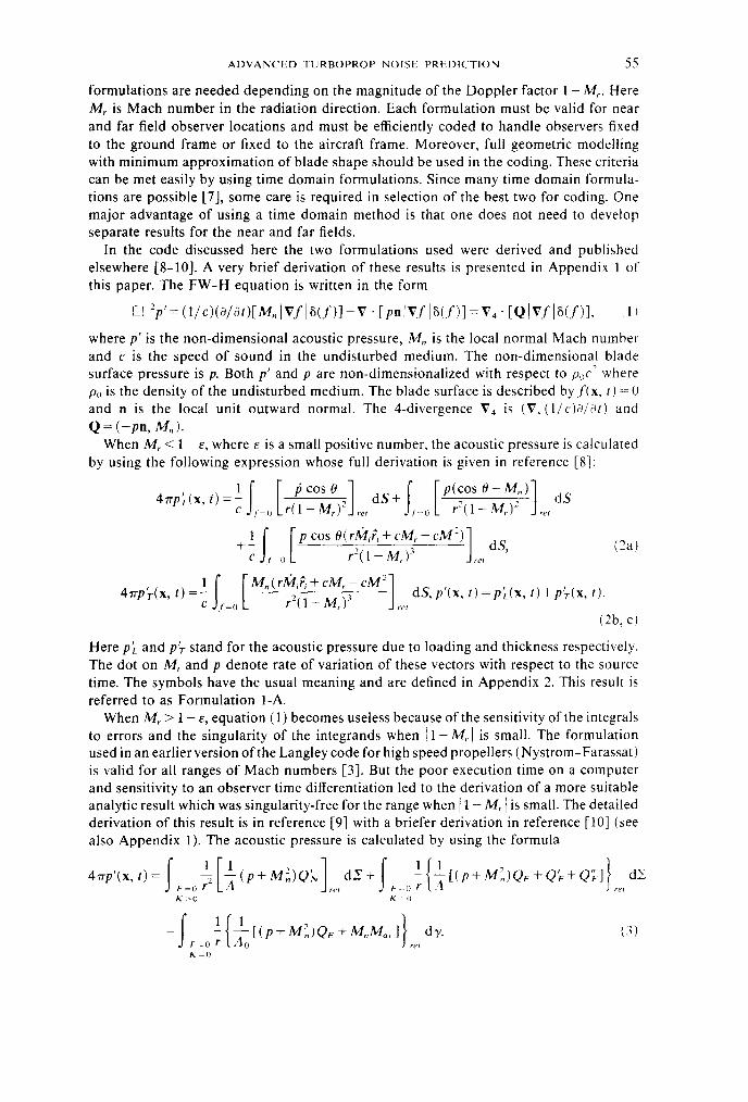
As an example of the precision of the present emission time routine, a particularlydifficult case of finding the emission times of a small segment of the blade leading edgewill be considered now. This segment, which has both single and multiple emission timesat the selected observer time, is moving at supersonic helical speed. Its operating conditionis recorded in Table I. An advanced blade planform design is used. Figure 4 shows theemission time (or times) versus distance along the edge. The emission times of about 100points along this line segment were calculated for this plot at a single observer time. Itis seen that the inboard portion of the line segment has a single emission time while the

58

59ADVANCED TURBOPROP NOISE PREDICTION

TABLE I

Blade data and operating conditions

Design SR-3No. of blades 8Radius (m) 0 317RPM 7569Blade angle, 3/4 radius (degrees) 58-9Advance ratio 3 030Tip helical Mach number 1-134Forward speed (m/s) 242 3Horsepower 223 7Power coefficient 1 828

5

4

E 30

vl2

1

0 96 097 0 98 099Sponwise co-ordinote

1 00

Figure 4. A test of the emission time calculation routine. The emission time of points on a segment of leadingedge at the tip (for a fixed observer time) is plotted versus radial distance. The straight part of the curve hasa very small slope and is not constant. Conditions corresponding to microphone 4.

rest of the segment has three emission times. Note that the part of the curve that lookslike a straight line has a small slope. The smoothness of these two pieces of curves inFigure 4, which are not smoothed numerically, is an indication of precision of the emissiontime routine.

3.3. CRITERION FOR SELECTION OF FORMULATION

An automatic decision making process must be used for each panel in the supersonicportion of the blade as to the type of Formulation (1-A or 3) for noise prediction. SinceGauss-Legendre integration is used exclusively for Formulation I-A, i.e., for subsonicpanels, the nodes for Gauss-Legendre (G-L) integration are first determined for eachcoarse panel as shown in Figure 3(b). The number of these nodes can be specified from9(3 x 3) to 100(10 x 10). If a node on a panel has multiple emission time, Formulation 3is used for that panel. Only if all nodes have single emission time and if M, < 1- F ateach node at its emission time, then Formulation 1-A is used. Formulation 3 is used asfollows. The coarse-sized panel is divided into smaller fine-sized panels as shown inFigure 3(c). Equation (3) is used by replacing dY/ A by c dr dF/sin 0 from equation(A8). This kind of integration over the 1-surface is known as the collapsing spheremethod. Again considerable care is required to extend the source time integration tocapture all the d-surface area of a panel. In particular, this surface can be more thanone piece and all the pieces must be included in the integration.

<Zz:::

F.

F. FARASSAT, S. L. PADULA AND M. H. DIUNN

Figure 5 shows panels for which Formulation 3 is used at three observer times markedon the pressure signature also shown in the figure. The signature is for one blade only.The panels shown are the coarse panels introduced above. In a typical calculation, thecoarse panel size is generally much larger than those shown in Figure 5. For completeness,it is mentioned that the operating conditions used in this figure correspond to Table Iand the observer position is at microphone 4 (see Table 2).

3.4. MOTION OF THE OBSERVER

The acoustic equations of this paper are derived in the frame fixed to the medium.That is, x in p'(x, t) is in the ground-fixed frame. If x is the observer variable in the framefixed to the aircraft moving at steady forward velocity V,, then

p (x, t ) = p (x,,+ V Ft, t )

where x0 is the observer position in the ground-fixed frame at time t = 0. This transforma-tion is used to find the acoustic waveform in the moving frame. In practice the implementa-tion of this transformation is very easy [3].

TE

{'L E

Time 1

0'-i

Time 2

Time 3

Figure 5. Panels used in Formulations 3 corresponding to three observer times marked on acoustic pressuresignature. Single blade.

TABLE 2

Boom microphone positions

Microphone no. Radial distance (in) Axial distance (m)

1 0 824 0 3053 0 824 -0 0084 0 824 -0252

Convention for axial distance: positive ahead of the disk negative behindthe disk.

60


3.5. UNSTEADY LOADING NOISE

The unsteady loading noise is calculated by specifying the blade surface pressure p asa function of time in the input data. The rate of change of the surface pressure withrespect to time, fi, must be calculated from p. Both of the formulations used here (1-Aand 3) have a term involving p. It must be noted that interpolations in the surface variablesand time of p are required to evaluate the integrands of the acoustic results. Obviously,more time is spent in the computer for unsteady blade loading than for the steady case.

3.6. CONTRA-ROTATING PROPELLERS

The prediction of the noise of contra-rotating propellers can be accomplished as follows.For a single rotor, the observer location is specified in a frame whose origin is at the diskcenter (i.e., where the pitch change axis intersects the propeller axis). For contra-rotatingpropellers, two sets of calculations must be performed with the observer specified at thecorrect position in the frame of each rotor. It must be mentioned that the observer timeorigin (time t = 0) is the same in all frames, so that simple superposition of pressuresignatures from each rotor gives the overall acoustic pressure signature. The aerodynamicinput data should obviously include the blade to blade interaction.

3.7. THE OUTPUT DATA

The acoustic pressure signature of one blade for period T corresponding to one completerevolution, is calculated first. For B blades, this signature is shifted by T/B seconds forB times. The overall acoustic signature for B blades is the sum of the signatures overany length of time of duration T/B. Following this, discrete Fourier analysis is used toobtain the acoustic spectrum.

4. COMPUTATIONAL GRID SIZE STUDY AND COMPARISION WITH AN EARLIERLANGLEY CODE

As mentioned in the previous section, the initial step in the computation is segmentingthe blade surface into coarse-size panels. If Formulation 3 is to be used for a panel,further subdivision into fine-size panels is made. Too large a panel size results incomputational errors while too fine a panel size results in excessive computer time.Furthermore, since Formulation 3 uses more time to execute on a computer than Formula-tion 1-A, because of the total number of operations needed per observer time, it is desirableto reduce the number of panels when using Formulation 3. This is controlled by the sizeof the parameter E. In this section the effects of grid size and e on the execution timeand on the acoustic pressure signature and spectrum are studied. In addition, the con-sistency of Formulations 1-A and 3 versus Formulation I used in the Nystrom-Farassatcode [3] is established in this section.

All the data presented are for the demanding case of an advanced propeller with sweptblades. The blade planform is shown in Figure 3. The blade form curves were shown inreference [3]. The operating conditions and some design data are presented in Table 1.The operating conditions pertain to a flight test in which the propeller was flown on apylon fixed on the top of the fuselage of a jet powered aircraft. The microphones weremounted on a boom held above the propeller (see Figure 6). The microphone positionsare given in Table 2. Because of a malfunction in the test, microphone number 2 dataare ignored. In the discussions of this section all calculations are for microphone 4 whichis behind the propeller disk. This position is chosen because during development of thecode more difficulties were encountered here than the other two microphone positions.All predictions are performed with the use of the full surface results of Formulations l-A

61

F FARASSAT, S. L PADULA AND M. H. DUNN

Figure 6. The test set-up and boom microphones.

and 3. The blade surface pressure was obtained from a code by using Denton's scheme[11]. Figures 7(a) and (b) show the distribution of the upper and the lower pressure onthe blade, respectively, in perspective. Note that the vertical scale is the pressure and thecomputational (rather than the physical) grid system is used for chordwise and spanwisedirection. The blade sweep is, therefore, not shown in this figure. Figure 7(c) and (d)shows the same data in contour plot form. Figure 7(e) shows the chordwise pressuredistribution at several radial stations.

Four grid sizes were selected as shown in Table 3. Grids A, B, and C refer to thosecoarse panels shown in Figure 8. The fine grid refers to division of coarse panels, i.e.,IO x 10 means that a coarse-sized panel is further divided into 10 equal chordwise and10 equal spanwise divisions. The value of E is taken as 0.05 and a 7 x 7 Gauss-Legendreintegration scheme (for Formulation 1-A) is used in all calculations. In the Table 3, therelative cost of execution on a computer is also given. The execution time of grid system3 was assumed as the unit time for the study of relative computation time. This gridsystem appears to be the best for noise prediction based on the present code. Table 4shows the acoustic pressure spectra (re 20 lPa) for the noise components and the overallsound pressure level at microphone 4 for the four grid systems of Table 3. Figure 9 showsthe corresponding acoustic pressure signatures. It is assumed that the smallest grid system4 is the most accurate of all calculations and therefore it is used to evaluate other grid sizes.

Grid system 1 gives quite poor OASPL and spectrum. Also the acoustic pressuresignature is considerably different from Figure 9(d). For this reason, system 1 is judgedunacceptable. Grid system 2 gives a good OASPL. The first nine harmonics are within2 dB and several of the harmonics are within I dB of those of grid system 4. The acousticpressure signature shows noticeable similarity with that of grid system 4 but is much lesssmooth. This grid system is judged acceptable if only the first few harmonics are required.Grid system 3 gives a good OASPL. The acoustic spectrum agrees within I dB of that ofgrid system 4 up to the 11th harmonic and for the remaining harmonics the agreementis within 2 dB. The acoustic pressure signature with minor differences is also very similarto that of grid system 4. In view of the above results and the much lower execution timefor grid system 3 as compared to grid system 4, the former grid is judged as the one mostsuitable for noise calculations.

The next study is on the selection of the value of £ which determines the choice offormulation for panels. In this connection, it must be mentioned that the numerical lineand surface integration schemes used in Formation 3 are less accurate than Gauss-Legendre scheme used in Formulation 1-A. Also as mentioned earlier, small £ is favoredto reduce execution time. However, because of the large size of panels used in the latter

62


Cantaur from-6000 ta 13000(Pa) Cantour from -5000 to 23000(Pa)Contour interval is 1000 (Pa) Contour interval is 1000 (Pa)

Tip Tip

L N!H-6814 5 781

4'.!-.1 . 0- o r

0 00

IC,

Cf ij C Aa'

Root Root

(c) (d)

Figure 7. Blade surface pressure. (a) and (b) 3-D relief (c) and (d) constant pressure contours, Pa; (a) Uppersurface; (b) lower surface; (c) upper surface; (d) lower surface; (e) chordwise pressure distribution.

case, there is the possibility of missing regions of multiple emission time for these panelsif £ is too small. This is because of the discrete nature of the criterion for selection offormulation.

Three values of £ were assumed for this study, 0-05, 0-1 and 0 2. Grid system 3, Table3, was used for all calculations. Compared to that for - = 005, the relative executiontimes for £ = 0 1 and 0 2 are 1-04 and 1 31 respectively. Table 5 shows the acoustic spectraat microphone 4 for a = 01 and 0-2. The case for £ = 0-05 is shown in Table 4 and isused as the reference for comparison. The acoustic pressure signatures corresponding toTable 5 are shown in Figure 10. It is seen that the OASPL of all the cases are within0.1 dB of each other. For £ =0'05 and 0.1 the acoustic spectra are within 0'5 dB up tothe 11th harmonic. Thereafter, deviation of up to 2 dB are observed but in most casesdeviations are smaller. Upon comparing the cases £ = 0'05 and 0-2, it is seen that theacoustic spectra are within 0'5 dB up to the 7th harmonic and the remaining harmonics

63

I

P

F FARASSAT, S. L. PADULA AND M. H. DUNN

Pressure

(e)

Figure 7. continued

TABLE 3

Grid system used in study of conference and computation time

RelativeGrid system Coarse grid Fine grid computation time

I A 5x5 0 272 A 10x 10 0 333 B lox10 1*004 C lox 10 3-47

are within I dB deviation. The acoustic pressure signatures for the three cases look verysimilar in detail. Case £ = 0 05 was selected to reduce computation time.

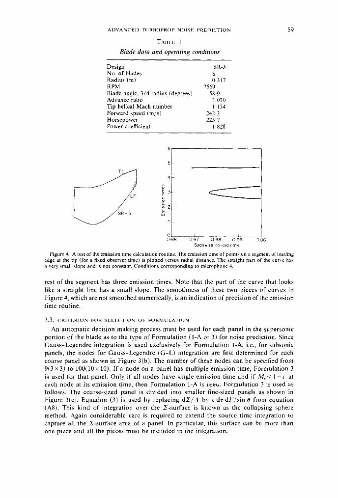
The output of the present code is now compared to that of an earlier code Nystrom-Farassat of NASA Langley. Identical input data were used in the two runs. The aero-dynamics input data to both codes, however, is similar to that of reference [3] withappropriate correction for horsepower. The full surface option of the codes were used.Figure 11 shows the acoustic pressure signatures and spectra for microphone 4. Onestriking difference is the high frequency oscillations due to numerical errors seen in thesignatures of the old code. However, it is obvious that the signatures have quite similarcharacters. The acoustic pressure spectra, except for higher harmonics, are also verysimilar. The deviations in high harmonics are caused by numerical errors of the old code.When the results of both codes ar compared it is obvious that the new code introducesan improvement over the old code. One major advantage of the present code is that inthis example the execution time was about five times faster than Nystrom-Farassat code.

5. COMPARISON WITH MEASURED DATA

In this section the theoretical prediction from the present code is compared withmeasured data for the test discussed in the preceeding section. Both the waveforms andacoustic spectra are used for comparison. It is very difficult to find experimental propeller

64


Subsonic | Supersonic

A

8

C

Figure 8. Grids used in grid size study.

acoustic data which is not contaminated by other physical effects such as reflections fromhard surfaces nearby and fuselage boundary layer propagation. Thus, the present noiseprediction code should be supplemented with other codes to include additional physicaleffects observed in the experiments. It was not possible to include quantitatively theseeffects with precision in the cases presented here. The sources of error are pointed outwhere they could be identified.

Before presenting the results of the calculations, two comments on the aerodynamicinput data, Figure 7, and the microphone boom reflection correction are in order. Theoriginal aerodynamic prediction code underestimated the absorbed power by about 25%.For this reason the predicted blade surface pressure was corrected by multiplying it bya linear function of radial position which decreased to the value of one at the tip. Therequired slope of this function is actually very small. Although the pressure distributionof Figure 7 seems reasonable, some numerical experiments with the present acoustic codehave shown that perhaps the actual chordwise distribution in the outboard region of theblades in the test is different from predicted. There is some experimental evidence fromflow visualization that there may be a leading edge vortex in the outboard region of theblade. This would change the chordwise pressure distribution particularly at the leadingedge (private communication, D. B. Hanson, 1986).

The microphones used in the test were flush mounted on the boom and were 1/8 inchin diameter. The influence of the boom on microphone measurements can be estimatedby using the results of Morse [12] on scattering from cylinders. However, the estimation

65


TABLE 4

The acoustic pressure spectra at boom microphone 4 for grid systems of Table 3; boomreflection correction is not included; E = 005

Grid system IHarmonic

Thickness Loading OverallFrequency noise noise noise

Number (Hz) (dB) (dB) (dB)

l 1009 20 147 43 139 75 147 062 2018 39 133 76 13490 132 573 3027 59 129 06 130*09 128-774 4036 78 127 35 126 58 130*845 5045 98 132 90 123 22 130 546 6055 17 127 45 120 77 126*327 7064-37 13193 121 52 130 498 8073 56 12467 110 38 124 199 9082 76 123 96 117 08 119 75

10 1009195 12155 115 93 123-6211 11101 15 122 24 109 98 123 3912 12110 34 125 27 110 34 123 6313 13119 54 119 31 109 44 121*8214 14128 73 120 55 111 17 117 2915 15137 93 118 51 9159 118 32

OASPL 147T80

Grid system 3Harmonic

Thickness Loading OverallFrequency noise noise noise

Number (Hz) (dB) (dB) (dB)

1 1009 20 138 15 139 04 138 812 2018 39 135*90 133-97 136 203 3027 59 132 00 128 46 130 634 4036 78 129 49 125 16 127 605 5045 98 128 41 123 01 126 826 6055 17 127 94 120 75 127 227 7064 37 126418 118 11 124 668 8073 56 124*32 116 03 121 959 9082-76 122 40 114*67 120 75

10 1009195 12063 113 14 119 8111 11101 15 120 34 110 89 119 1712 12110 34 118 26 108 33 116 4313 13119 54 115 88 107 12 1147514 14128 73 115-01 104 53 114-5715 15137 93 11483 103 19 11431

OASPL 141-93

Grid system 2

Thickness Loading Overallnoise noise noise(dB) (dB) (dB)

140 64 138-76 140 39135*41 134 13 135-1513177 128-83 129 87127*59 125-53 126-15129 90 122 95 128 65127-42 120 17 125 12128 14 120 85 126-99124 54 11181 123 94124 21 115 95 120 28122-82 115 78 124 08120 54 106 02 119 2611783 11084 11560116 14 105 90 114 77116 34 108 70 115 02114 91 87-51 114 55

OASPL 142 64

Grid system 4

Thickness Loading Overallnoise noise noise(dB) (dB) (dB)

137 85 139 03 138 70135 73 133 93 135 92132 10 128-55 130 95129 79 125-19 127-58128-38 122-94 126 86127 74 120 69 127-02126 24 118-04 124 68124 30 116-07 122 23122-42 114-55 120-83120 98 113-05 120-30120-87 110-73 120-13119-47 108-41 118-36116-47 107-30 115-64115-88 106-23 115-60115-66 103-85 114-88

OASPL 141-86

66


300 (a) 400 (b)

0 200

300 0

-600 -200

900 - \-400

-600-1200

a -800

.~400 (c) 400 (d)

200 200

0 0

-200 -200

- 400 -400

-600 -600

- 800 I-8000 02 04 06 08 1 0 0 0 2 0 4 0-6 0-8 10

Time / Period

Figure 9. Acoustic pressure signatures corresponding to grid systems 1-4. Microphone 4, E 005, period0 991 ms. (a) Grid system 1; (b) grid system 2; (c) grid system 3; (d) grid system 4.

requires some approximations whose influence on the estimation cannot be ascertained.One of these approximations is the direction of propagation of sound which, because ofproximity of the source and microphones, cannot be determined. It was therefore thoughtreasonable to take a correction of 4 dB for all microphones and all the harmonics of thespectra. Similarly, predicted acoustic pressure signatures were multiplied by the factor1-58. This was the correction suggested and used by Brooks and Mackall [13]. It is knownthat this correction is a function of frequency [ 12]. The proposed correction must thereforebe regarded as approximate. In fact, the estimation of what the microphones measure isvery difficult because of the nature of the source (distributed), refraction of the sound inthe fuselage boundary layer and its subsequent reflection from fuselage surface. Thesolution of such problems requires development of other computer codes. The theory forprediction of the boundary layer refraction effect has been given by McAninch [14],McAninch and Rawls [15] and Hanson and Magliozzi [16].

Figure 12 shows the measured and predicted acoustic pressure signatures and spectrafor microphine 1. The measured and predicted signatures are similar but there is anoverprediction. A similar trend is also seen in the spectra. Prediction based on Hanson'smethod for one harmonic from reference [13] agrees well with prediction from the presentcode. No information on assumed blade loads is given in reference [13]. It is known thatin Hanson's method the thickness and loading sources are located on a helicoidal surfacewhich is infinitely thin. Quadrupole sources were also used in acoustic calculations ofreference [13] but they make only a small contribution. It is interesting to note that thisboom microphone is significantly influenced by the presence of the fuselage. A measureof this influence can be obtained by using an image propeller symmetrically located with

67


TABLE 5

Acoustic pressure spectra at boom microphone 4for = 01 and E = 02; compare with resultsof Table 4, grid system 3; grid system 3 is used in these calculations; boom reflection

correction is not included.

Grid system 3, £=

HarmonicThickness Loading

Frequency noise noiseNumber (Hz) (dB) (dB)

1 1009*20 137 86 139 032 2018 39 136 42 133*883 3027 59 13179 128 444 4036 78 129 56 125 165 5045 98 128 86 122-936 6055 17 127'67 120'887 7064 37 126 56 118 038 8073 56 124 46 116'159 9082-76 122 65 114 65

10 1009195 12102 113'1211 11101'15 12025 111 1712 12110 34 119'89 108 3313 13119 54 115 01 106 9814 14128 73 115 08 104 9915 1513793 115 35 101 28

OASPL

400

, 200

,I 0O

C -200

-4000'I

-6001

-800 L0 02 04 06 08

Grid system 3, E = 0 2

Overall Thicknesnoise noise(dB) (dB)

138 57 137 90136 57 135 88130 29 132 02127 59 129 64127 21 128 80127-00 127 97125 04 126 49122 06 124 68121 25 122 46120 30 121 00119 54 120 56118 52 118 6511306 11598115 34 115 19114 38 115 31141 93

1-0 0Time/Period

is Loadingnoise(dB)

139 06134 06128 61125-27123 13120 91118 32116 26114 69113 29111 02108 89106 82105 01102 69

OASPL

02 0-4 06 08

Figure 10. Acoustic pressure signatures corresponding to (a) E =

(b) E= 0*2.0 1 and (b) 0 2. Grid system 3. (a) E =0'1;

respect to the tangent plane at the point where the radial line joining the fuselage centerand propeller center meets the fuselage. It must be mentioned that the fuselage curvatureeffects are significant and thus this study must be considered qualitative in nature. Figure13 shows this arrangement.

Figure 14 shows the corrected acoustic pressure signature and spectrum of the imagepropeller at microphone 1. It is seen that the image propeller alone generates as muchnoise as is measured by the microphone. Of course, refraction through fuselage boundarylayer and fuselage curvature effects on reflection are not included in this study. Neverthe-less, this study shows that propeller noise measured at the boom microphone 1 is highly

Overallnoise(dB)

138 51136 10130 78127 54127 37127 12124 93122 71120 93120 39119 53117 11115 19114 81114 75141 81

1 0

68

69ADVANCED TURBOPROP NOISE PREDICTION

140

1 130

zL 1200N 11 0

co 100

-J 90a.cv 80

70

Tine / Period

I

KV

5 10 15 20 25 30

Harmonic number

(c)

Figure 11. Comparison of outputs of the present code with Nystrom-Farassat code. (a) Thickness noise; (hbloading noise; (c) overall noise. Period 0.991 ms. V, Nystrom-Farassat [3]; |, present code.

contaminated by the presence of the fuselage. This effect does not appear to be as

significant for the other two microphone positions although the signatures seem to show

this effect to some extent. Figure 15 shows the corrected acoustic pressures and spectra

of the image propeller at microphones 3 and 4. Again, the readers are cautioned thatthese results must be considered as qualitative.

Figure 16 shows the predicted and measured acoustic pressure signatures and spectra

for microphone 3. The predicted acoustic pressure signature is very similar to the measuredsignature. A sharp positive peak in predicted signature is most likely wiped out in

measurement due to the finite size of the microphone. The need for microphone size

correction in another situation has been discussed by Atvars et al. [171. The removal of

this peak reduces the high harmonics of predicted spectrum and improves the agreementbetween the measured and predicted spectra. The first three harmonics and the fifthharmonic values are within 2 dB of the measured values. When the fuselage reflection

0~a-

0

EdC,n7T;

i


03

Vqa;

En

.-P

a-

-aU,ra~

InV

0.

0C)

0

-500

-O 150a-Z- 1400N~ 130

a 120

-J 110V- . -

JULI. . . . . . . . . I I I I I I I I

Time / Period

0 5 10 15 20 25 30

Harmonic number

Figure 12. Comparison of the measured and predicted acoustic pressure signatures and spectra of boommicrophone 1. Theoretical prediction corrected for boom reflection. (a) Experimental; (b) theoretical; (c)spectrum. V, experimental; |, theoretical; OI, Hanson's method. Period = 0991 ms; BPF = 1009.2 Hz.

Propeller< disk

'e

-yongeflp rcoe

Fuseloge(Jetstor)

Figure 13. The propeller disk and its image used for fuselage reflection study.

(a)

I IL I I I J i I I I I

I- (c)

- I !J'I 117 Ii iI i I

.111 H J.

70


a-0

-5000 ) 2 3 4

Time/Period150 -

X140-

o IZ0N130w

120~110 _ _ _ _ _ _ _ _ _ _ _ _ _

0 5 10 15 20 25 30

Harmonic number

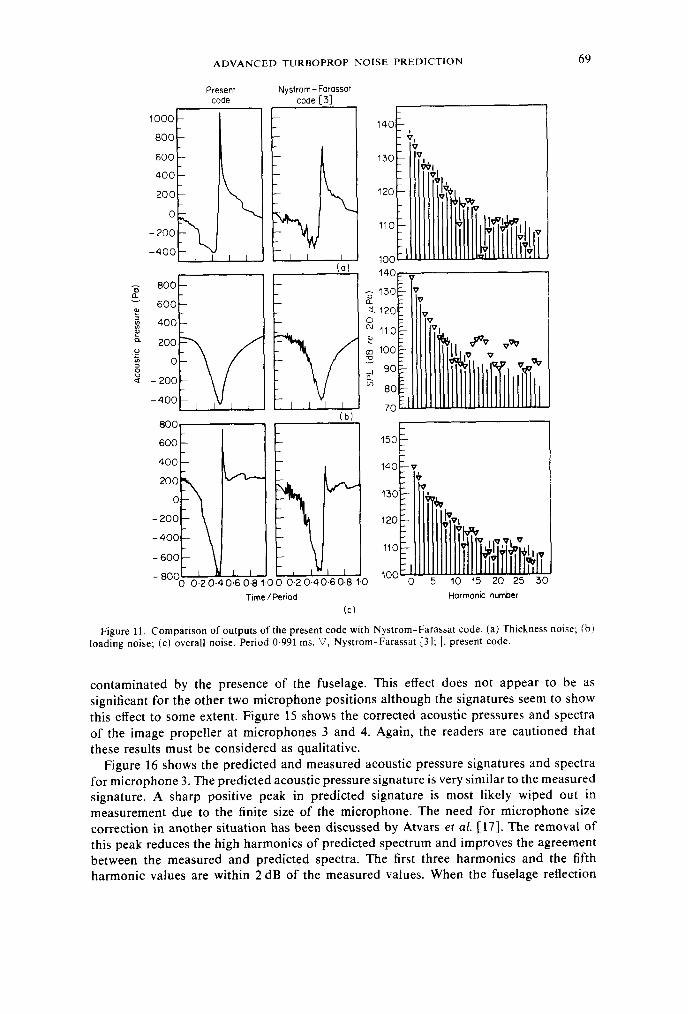
Figure 14. The acoustic pressure signature (a) and spectrum (b) of image propeller at microphone I correctedfor boom reflection. Period = 0-991 ms; BPF = 1009 2 Hz.

and boom effects are considered, the agreement between the two spectra is good. Predictionof the first harmonic based on Hanson's method [13] agrees slightly better than that bythe present method, perhaps due to differences in the geometric and aerodynamic inputdata.

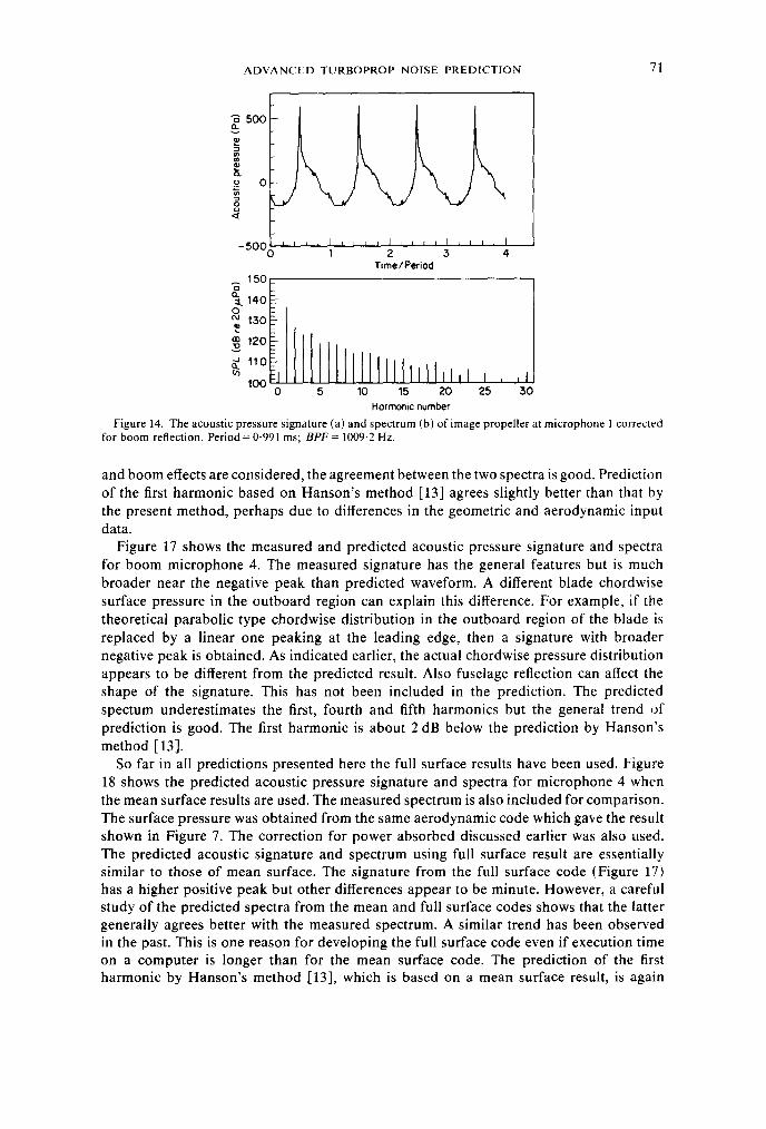
Figure 17 shows the measured and predicted acoustic pressure signature and spectrafor boom microphone 4. The measured signature has the general features but is muchbroader near the negative peak than predicted waveform. A different blade chordwisesurface pressure in the outboard region can explain this difference. For example, if thetheoretical parabolic type chordwise distribution in the outboard region of the blade isreplaced by a linear one peaking at the leading edge, then a signature with broadernegative peak is obtained. As indicated earlier, the actual chordwise pressure distributionappears to be different from the predicted result. Also fuselage reflection can affect theshape of the signature. This has not been included in the prediction. The predictedspectum underestimates the first, fourth and fifth harmonics but the general trend ofprediction is good. The first harmonic is about 2 dB below the prediction by Hanson'smethod [13].

So far in all predictions presented here the full surface results have been used. Figure18 shows the predicted acoustic pressure signature and spectra for microphone 4 whenthe mean surface results are used. The measured spectrum is also included for comparison.The surface pressure was obtained from the same aerodynamic code which gave the resultshown in Figure 7. The correction for power absorbed discussed earlier was also used.The predicted acoustic signature and spectrum using full surface result are essentiallysimilar to those of mean surface. The signature from the full surface code (Figure 17)has a higher positive peak but other differences appear to be minute. However, a carefulstudy of the predicted spectra from the mean and full surface codes shows that the lattergenerally agrees better with the measured spectrum. A similar trend has been observedin the past. This is one reason for developing the full surface code even if execution timeon a computer is longer than for the mean surface code. The prediction of the firstharmonic by Hanson's method [13], which is based on a mean surface result, is again

7 1

I I I I


50.

0

2 3 4Time/Period

- 150a.:. 140

q,130

120

110

0 5 10 15 20 25 30Harmonic number

-s 1000 (a)

! 500 -

CF 0

u -5000

o -1000 , , , I I l , I l0 1 2 3 4

Time/Period150

t 1 4 0L

0)

co 120

1100

0 5 10 15 20 25 30Harmonic number

(bW

Figure 15. The acoustic pressure signatures and spectra of image propeller at microphones 3 and 4. Correctedfor boom reflection. (a) Microphone 3; (b) microphone 4. Period =0 991 ms; BPF = 1009 21 Hz.

higher than that predicted by the current code as seen in Figure 18. Once more the effectof differences in input data cannot be assessed.

A recent paper of Tam and Salikuddin [18] has been brought to the attention of theauthors by one of the referees. The referee believes that "Tam and Salikuddin use thesame data as the present authors and provide solid explanation for the two effectsmentioned on page 17 (of the original manuscript): reduction of the positive pressurepeak and widening of the negative part of the pressure pulse". Tam and Salikuddin haveused the weak shock wave theory of Whitham to account for steepening of the waveformobtained from the linear theory. In their calculations, the starting waveform is taken atabout one radius distance from the center of the propeller. However, they have assumedthat only the far field terms of linear acoustics should be used in calculating the startingwaveform. This assumption in itself casts serious doubt on their analysis. Their theoryshould be of value for propagation to larger distances starting from the true far fieldlocation. The reduction of the positive peak that the referee mentioned is most likely dueto the fact that Tam and Salikuddin constructed their waveform by a frequency domain

72


Time/Period

5 10 15 20 25Harmonic number

Figure 16. Comparison of measured and predicted acoustic pressure signatures and spectra at boom micro-phone 3. Theoretical prediction corrected for boom reflection. (a) Experimental; (b) theoretical; (c) spectrum:V, experimental; |, theoretical; C, Hanson's method. Period = 0.991 ms; BPF = 1009 2 Hz.

method and have not used a sufficient number of harmonics. As mentioned earlier, thebroadening of the negative peak, which is seen also in Tam and Salikuddin's linear results,may be due to the differences in aerodynamic or perhaps geometric input data from thoseof the present paper. Unfortunately, no information about the input data or correctionsto the data have been included in reference [18] to check the validity of this assertion.

6. CONCLUDING REMARKS

In this paper the development of a computer code for prediction of the noise of highspeed propellers has been presented. This code is based on two recent acoustic formula-tions, each of which is suitable for a different range of the Doppler factor of the sourceson the blades. The use of these formulations plus improvements in algorithms employedin coding have resulted in great increase in accuracy and speed of execution on a computer.

0)

0

4

a.

a-

Zj 14'0" 13

10CD 12'

(In

10'

U

V I I VI

0, III I II I

0 30

73


<, 15000-500

00-(b-500

-2000

150 ~ Time/Period c-150-

CJ 0 150

0ed 5 10 51 20 25 3

It must be mentioned that this code should be supplemented by other aerodynamicand acoustic codes (e.g., boundary layer refraction, atmospheric prop~agation, groundeffects and fuselage reflection) for prediction of the noise of a propeller in realistic cases.As such, the development of the present code is just one step in designing a sophisticatedmulti-module propeller noise prediction program which includes all the physicalphenomena existing in actual flight conditions.

One use of the code which has not been emphasized earlier is for structural acousticpurposes. Some of the recent fuselage propagation codes require detailed surface loadinginputs that can only be supplied by an acoustic code such as described here [19]. Thecurrent design philosophy for propeller driven airliners includes aft-mounted engineswhere propeller tip clearance from the fuselage is small. Both single rotor and contra-rotating propellers are proposed for propulsion. Near field computation is essential forfuselage structure in the vicinity of the propeller. The present code is highly suitable forthis purpose.

ACKNOWLEDGMENTS

The authors would like to thank Mr Bruce Clark of NASA Lewis Research Center forhis help in supplying aerodynamic data and Messrs B. M. Brooks and B. Magliozzi of

74


500

0)

< -500

S -10000

-1500

Time/Period150

(b)140 @V

a. 0o. 1010

~~0120c. - { V .110

1000 5 10 15 20 25 30

Harmonic number

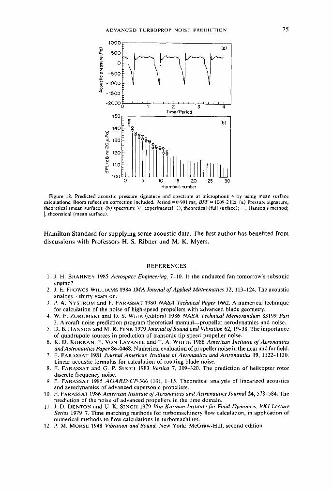
Figure 18. Predicted acoustic pressure signature and spectrum at microphone 4 by using mean surfacecalculations. Boom reflection correction included. Period = 0 991 ms; BPF = 1009.2 Hz. (a) Pressure signature,theoretical (mean surface); (b) spectrum: V, experimental; 0, theoretical (full surface); C, Hanson's method;l. theoretical (mean surface).

Hamilton Standard for supplying some acoustic data. The first author has benefited fromdiscussions with Professors H. S. Ribner and M. K. Myers.

REFERENCES

1. J. H. BRAHNEY 1985 Aerospace Engineering, 7-10. Is the unducted fan tomorrow's subsonicengine?

2. J. E. FFOWCS WILLIAMS 1984 IMA Journal of Applied Mathematics 32, 113-124. The acousticanalogy-thirty years on.

3. P. A. NYSTROM and F. FARASSAT 1980 NASA Technical Paper 1662. A numerical techniquefor calculation of the noise of high-speed propellers with advanced blade geometry.

4. W. E. ZORUMSKI and D. S. WEIR (editors) 1986 NASA Technical Memorandum 83199 Part3. Aircraft noise prediction program theoretical manual-propeller aerodynamics and noise.

5. D. B. HANSON and M. R. FINK 1979 Journal of Sound and Vibration 62, 19-38. The importanceof quadrupole sources in prediction of transonic tip speed propeller noise.

6. K. D. KORKAN, E. VON LAVANTE and T. A. WHITE 1986 American Institute of AeronauticsandAstronautics Paper 86-0468. Numerical evaluation of propeller noise in the near and far field.

7. F. FARASSAT 1981 Journal American Institute of Aeronautics and Astronautics 19, 1122-1130.Linear acoustic formulas for calculation of rotating blade noise.

8. F. FARASSAT and G. P. Succi 1983 Vertica 7, 309-320. The prediction of helicopter rotordiscrete frequency noise.

9. F. FARASSAT 1985 AGARD-CP-366 (10), 1-15. Theoretical analysis of linearized acousticsand zerodynamics of advanced supersonic propellers.

10. F. FARASSAT 1986 American Institute of Aeronautics and Astronautics Journal 24, 578-584. Theprediction of the noise of advanced propellers in the time domain.

11. J. D. DENTON and U. K. SINGH 1979 Von Karman Institutefor Fluid Dynamics. VKI LectureSeries 1979-7. Time marching methods for turbomachinery flow calculation, in application ofnumerical methods to flow calculations in turbomachines.

12. P. M. MORSE 1948 Vibration and Sound. New York: McGraw-Hill, second edition.

75


13. B. M. BROOKS and K. G. MACKALL 1984 American Institute of Aeronautics and AstronauticsPaper 84-0250. Measurement and analysis of acoustic flight test data for two advanced designhigh speed propeller models.

14. G. L. McANINCH 1983 Journal of Sound and Vibration 82, 271-274. A note on propagationthrough a realistic boundary layer.

15. G. L. McANINCH and J. W. RAWLS, JR 1984 American Institute of Aeronautics and Astronautics84-0249. Effects of boundary layer refraction and fuselage scattering on fuselage surface noisefrom advanced turboprop propellers.

16. D. B. HANSON and B. MAGLIOZZI 1985 Journal of Aircraft 63-70. Propagation of PropellerTone Noise Through a Fuselage Boundary Layer.

17. J. ATVARS, L. K. SCHUBERT, E. GRANDE and H. S. RIBNER 1966 NASA CR 494. Refractionof sound by jet flow or jet temperature.

18. C. K. W. TAM and M. SALIKUDDIN 1986 Journal of Fluid Dynamics 164, 127-154. Weaklynonlinear acoustic and shock-wave theory of the noise of advanced high-speed turbopropellers.

19. L. D. POPE, E. G. WILBY and J. F. WILBY 1984 NASA CR 3813. Propeller aircraft interior noise.20. 1. M. GEL'FAND and G. E. SHILOV 1964 Generalized Functions (Volumne 1) Properties and

Operations. New York: Academic Press.21. R. P. KANWAL 1983 Generalized Functions-Theory and Technique. New York: Academic Press.22. F. FARASSAT 1983 American Institute of Aeronautics and Astronautics 83-0743. The prediction

of the noise of supersonic propellers in the time domain-new theoretical results.

APPENDIX I

In this appendix a brisk derivation of the theoretical formulations used in developingthe code reported here is given. Readers should consult original references for moredetailed derivation. Consider the wave equation

E -20 = (a/aXi)[QVf I6(f)], i=,...,4, (Al)

where xi, i = 1,. . . , 3 are the space variables and x 4 = ct. The summation convention oftensor analysis is used in this equation. As is obvious from the Dirac delta function 8(f),the moving source surface is described by f =0. The formal solution of equation (Al) is

4T <7i(X, ) = I- Qi |f Ie 8 8(f ) 8g) dy d T, (A2)

where g = r - t + r/ c, r x - y I and (x, t) and (y, T) are observer and source space-timevariables respectively.

It is a significant fact that the derivatives with respect to observer space variables inequation (A2) can be converted to observer time differentiation exactly. One utilizes therelation

a~i [ 1 aX [ ) ]~ - 2, i =1, . . ., 3, (A3)aXi r Jrax2where Pi = (xi - y )/ r, i = 1, . ., 3, is the unit vector in the radiation direction. U sing equation(A3) in equation (A2) results in

47ro(x, t)=--I (Q4 Qr) Vf 1(f)8(g) dy dr- Q-'Vf 6(f)b(g)dy d, (A4)4iix )X4 r J r2 1 ~bf5 yd,(4

where Qr = QiP,, i = 1,. . . 3. The interpretation of integrals involving products of deltafunctions has been given elsewhere [7, 20, 21]. Let the surface .: be described byF(y; x, t) = [f(y, T)],,, = 0; then equation (A4) can be written as

47+ (x, t) = J i [Q-] d 2 [A] dl, (AS)(1X4 F.0 r A Iret r A1 re

76


where

A2 = I+ M'-2M, cos 0. (A6)

In equation (1), Q = (-pn, Mj) so that the solution of equation (1), upon using equation(A5), is

4 ~p' I [Mn+p cos] d 1 [ dY (l7)1 d2'+ -I II f (A7C At F -r FL r P 4OS 1

This equation, referred to as Formulation 1, was coded in a high speed propeller noiseprediction program by Nystrom and Farassat [3] for both subsonic and supersonic sources.It is used in the ANOPP program [4] for supersonic sources only. It was also coded forhelicopter rotor noise prediction. The following relation was used to write equation (A7)in two equivalent forms for subsonic and supersonic sources [7]:

d2; dS c dT dF

4 I1-Mr sin ' (A8)

Here dr is an element of the curve of intersection of the surfaces f = 0 and g = 0.Because of excessive execution time on a computer and sensitivity to errors of numerical

differentiation of equation (A7), two different results were derived for subsonic andsupersonic sources. For the subsonic case, with the integration on the actual blade surfacebeing used (from equation (A8)), the time derivative of equation (A7) was taken insidethe first integral, resulting in equation (2) of this paper [8].

For supersonic sources, a singularity-free formulation is much more difficult to derive.In equation (1), Q is decomposed into two vector fields QN and QT normal and tangentto the surface f = 0 in four dimensions. Here QN and QT are [9, 10]

QN = -(l/a 2)(p+M2)(n, -M), QT= (I/C)M.(l -p)(Mnl). (A9abb)

Equation (1) then can be written, for an open piece of the surface, as

o2 p =V 4* [H(k)QN IVf 8(f)]±+V4 - [H(k)QT1Vf]8(f), (A10)

where k = 0 together with f = 0 define the edge of the open surface.The interpretation of the second term of equation (A10) is easy. The first term requires

a great deal of algebra. By using the Green function of the wave equation, an integral ofthe following kind is obtained:

I=f '(g) V4 [H(k)QNIVfIT]8(f)dydT+J -f ddYdT, (All)Jr r

where the second integral is of a conventional type involving 8(f)8(g) which results ina surface integral on the surface a1. By using an identity of generalized functions [22],the first integral can be written as the sum of two integrals involving 8(f)8(g) and8(f)8(g)8(k), respectively. The integral whose integrand has 8(f)b(g)8(k) gives the lineintegrals in equations (3) and (4). The complexity of these equations have come fromthe attempt to write each term of the final integrands in explicit forms for computercoding. It should be noted that a relation similar to equation (A8) exists for line sources,and which was utilized in coding [18]:

dy dl c drAo |Il-MA || cos |(A12)

77

F. FARASSAT. S L. PADULA AND M. H. DUNN

Here dl is the element of length of the edge of the open surface and 4' is the local anglethat the edge makes with radiation direction i.

APPENDIX 2: NOMENCLATURE

BI

b

C

F(y; x, t)F. (y; x, t)f(y, T) = 0, f(X, t) = 0

fm (y, T) = 0, f_ (x t) = 0

gH(k)Hhn

K(y; x, t) = 0k=0

MMP

M,

N

n, n7

PIPB(-, T)

Q N1

QF

Q'F

Q IF

QE

r, rr, r

S

ti

i = 1, 2 components of b along the direction of the principal curvatures;basis vectors assumed unit length=AM, +At,; b bb-vspeed of sound=f(y, t - rlc) = [fly, r)]e~fm(y, t -rl c) =[f- (y, r)]e

the equation of the blade surface in the frame fixed to the undisturbedmediumthe equation of the mean blade surface in the frame fixed to theundisturbed medium=7r - t + r/cHeaviside functionthe local mean curvature of the blade surface-AM, +Al cos 0=[k(y, 7-)]rel

the equation of a surface whose intersection with f = 0 produces a finiteopen piece of the blade surface by relations f = 0, k > 0(in dl) length variable along the trailing edge, along perimeter of airfoilsection, at blade inner radius or along shock traceslocal Mach number vector based on c, M. = M n, M, = M *the projection of the Mach number vector on the local plane normalto the edges (e.g., TE) of blade surface, M, I M, Ithe projection of M on the local tangent plane of the blade surface forfixed source time 7, M, = IM, |the four-dimensional unit vector normal to f(y, r) =0 described by(n, -M,)/a,,unit normal to f = 0, r-fixedacoustic pressure (non-dimensional)-p(y(-q, r), -) blade surf? e pressure described in a frame moving withthe blades (non-dimensional)=A[2A,(cos 0- M) + 1]

=-I2A2 - I2)M + I [ 4-2 -2Ab+ I +2AAl)rJ+2b Kb

+ KT1 1 t + K2 (T22 2Hh,= (A /0B - bWpB/ro-h + 2M,[(1/ c)(AM, -n- b) + K,/.I'BI + K2/LB2]

=(I/c)(M,- fi M,) + KMM2t-2HM2,

=(/c)(M,- n M,)+KMM21; KM is the average of the normal cur-vatures of the upper and lower blade surfaces in the direction of M,= A M.V + Ak_ M, = M v; M based on absolute velocity=x -y, r= IX -YIunit radiation direction vector r/rr vunit vector in the direction of the projection of i^ on the local planenormal to the edges (e.g., TE) of blade surface, 7-fixed(in dS) element of blade surface areaobserver timethe projection of the unit radiation direction vector i on the local tangentplane to f = 0, 7-fixed; not unit vector, It, I = sin 0

78


Greek symbolsa,,y

F

V46(f)

.1

,i

"A

V, Pj

Po

al, I, 0'22

ii, (2,K 1 , K2

KW, K,, Kb

AA,to

=(1 + M,,1 o o negeo ) (eg.(in dy) length variable along the intersection of an edge off = Xe.g.,TE) and the collapsing sphere g = 0(in dF) length variable of the arc of intersection of surfaces f 0 andg =0the 4-D gradient (V,, (l/c)a/aT), V, = (/aythe Dirac delta functionthe angle between n and rthe Lagrangian co-ordinate of a point on the surface f = 0=(1 4- M 2M cos 6)1/2

(A 2 +sin2 6)1 2[Mp cos2 q1 + (I Mp ir sin qj) 2

]l 21, 2 components of M, in the direction of principal curvatures; basis

vectors assumed to be of unit lengthunit inward geodesic normal: i.e., the surface vector perpendicular toan edge (e.g., TE) of the surface f = 0, --fixeddensity of undisturbed medium(in dl) surface area of F= 0the length parameter on f = 0 along btwo components of tensor (ttt,-MM, +t1 M,+Mt 1 )/A 2 ,the local angle between r and an edge off = 0=nXtoprincipal curvatures of the surface f = 0normal curvatures along M,, t,, and b, respectively=(cos 6 _ Mj/ 2=(cos 0+ M,,)/ 2

angular velocity

Other symbols are defined in the text.

79

advanced turboprop noise prediction...

Documents