AGRICULTURAL PRICES

AND MARKETS

AGRICULTURAL PRICES

AND MARKETS Sponsored by a Grant TÁMOP-4.1.2-08/2/A/KMR-2009-0041

Course Material Developed by Department of Economics,

Faculty of Social Sciences, Eötvös Loránd University Budapest (ELTE)

Department of Economics, Eötvös Loránd University Budapest

Institute of Economics, Hungarian Academy of Sciences

Balassi Kiadó, Budapest

AGRICULTURAL PRICES

AND MARKETS

Author: Imre Fertő

Supervised by Imre Fertő

June 2011

ELTE Faculty of Social Sciences, Department of Economics

AGRICULTURAL PRICES

AND MARKETS

Week 2

Demand for agricultural products

Imre Fertő

Literature • Tomek, W. G.–Robinson, K. (2003): Agricultural Product Prices.

Cornell University Press, Chapter 2–3

• Hudson (2007): Agricultural Markets and Prices. Blackwell,

Chapter 1

• Chai, A.–Moneta, A. (2010): Engel Curves. Journal of Economic

Perspectives, 24 (1) 225–240

• Bouamra-Mechemache, Z.–Réquillart, V.– Soregaroli, C.–

Trévisiol, A. (2008): Demand for dairy products in the EU. Food

Policy 33, 644–656

• KSH (2010): Development of food consumption, 2008

(Statisztikai tükör)

http://portal.ksh.hu/pls/ksh/docs/hun/xftp/stattukor/elelmfogy/elel

mfogy08.pdf

• Regmi, A.–Takeshima, H.–Unnevehr, L. (2008): Convergence in

Global Food Demand and Delivery. USDA, ERS, Washington,

ERR No. 56

Demand for agricultural

products • Different approaches of consumer behaviour

• The basics of demand theory

• Determining factors of demand

• Price elasticity of demand

• Income elasticity of demand

• Relationships between demand elasticities

• The pattern of food consumption

• The methodologies of demand analysis

• An empirical example: the Hungarian beer

consumption

Different approaches of consumer

behaviour • Rational choice

• Bounded rationality

– Searching information

– Processing information

• Impulsive behaviour

– Theory of rational addiction (Becker–Murphy)

• Behaviour based on habit

• Behaviour based on social status

– Veblen effect

– Snob effect

– Group effect

Demand theory • Utility

– The unit of the theory is individual

consumer or household

– Utility maximalisation with budget

constraints

– We do not measure the utility

– Two axioms

• Consumer prefer more to less

• Consumer will buy only at lower price

– Utility function

– Utility: the level of well-being or satisfaction

that an individual experiences

Demand theory • Indifference curves

– Set of goods, which has

the same utility for the

consumers

– Growing income implies

higher indifference

curve

– The rate of substitution

– Substitution effect (HH)

• Substitutes: –HH

• Complements: +HH

– Income effect

Price and income effects if price of

good 2 increase Substitution

effects

Income

effect

ÖH

Good 1.

superior

Q1↑ Q1 Q1↑

Good 1.

inferior

Q1↑ Q1↑ Q1↑↑

Good 2.

superior

Q2↓ Q2↓ Q2↓↓

Good 2.

inferior

Q2↓ Q2↑ Q2↑↓

Demand theory • Max(F,H) assuming

• Pf*F+PhH=Y

– U: utility

– F: food

– H: house

– Y= income

– Pf: price of food

– Ph: rent of houses

U=F*H+λ(Y-Pf*F+PhH)

• Take partial differential

• Partial differentials equal to zero

• Solve for F and H

• E.g.: U=f(F,H)

• 20F–H=1000

U=F*H+λ(1000–20F–H)

dU/dF=H–20λ=0

dU/dH=F–λ=0

dU/dλ=1000–20F–H=0

F=25, H=500

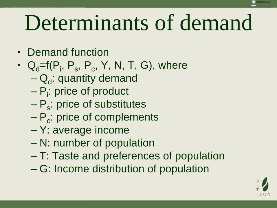
Determinants of demand • Demand function

• Qd=f(Pi, Ps, Pc, Y, N, T, G), where

– Qd: quantity demand

– Pi: price of product

– Ps: price of substitutes

– Pc: price of complements

– Y: average income

– N: number of population

– T: Taste and preferences of population

– G: Income distribution of population

How can various factors

affect on demand quantity – Pi: increase or decrease

– Ps: increase or decrease

– Pc: increase or decrease

– Y: increase

– N: increase

– T: change

– G: change

Demand elasticity • Own price elasticity

– If Ep<–1 elastic

– If Ep=–1 unitary elastic

– If Ep>–1 inelastic

– If Ep=0 perfectly inelastic

– If Ep=∞ perfectly elastic

)//()/(p QPdPdQE

)/()()/()( 10101010p PPPPQQQQE

Demand elasticity • But!

– Demand elasticity may change along

demand curve

– E.g. linear demand curve

– Q=10–P

– If P=5, then Ep=–1

– If P=8, then Ep=–4

– If P=4, then Ep=–0,25

Relationship between price

elasticity and total revenue • TR=P*Q

– dTR=Q*dP+PdQ (/TR)

– dTR/TR=Q/TR*dP+P/TR*dQ

– dTR/PQ=Q/PQ*dP+P/PQ*dQ

– dTR/PQ=dP/P+dQ/Q

– dTR/PQ=dP/P*(1+Ep)

• If

– Ep<–1, then total revenue grows

– Ep=–1 then total revenue is constant

– Ep>-1, then total revenue declines

Relationship between price

elasticity and marginal revenue • TR=P*Q

– dTR=Q*dP+PdQ (/dQ)

– dTR/dQ=Q*(dP/dQ)+P

– dTR/dQ=P*(1+Q/P*dP/dQ)

– dTR/dQ=P*(1+1/Ep)

• Amoroso-Robinson relation

• If

– Ep<-1, then marginal revenue decreases

– Ep=-1 then marginal revenue is constant

– Ep>-1, then marginal revenue increases

Cross price elasticity

• If Eij>0, then i and j are substitutes

• If Eij<0, then i and j are complements

• If Eij=0, then i and j are independent

• But!

• Income effect may cause complication

• Assume: share of i product is much higher in total expenditures than substitutes

• If price of product i is going up, then demand of product j may decline, thus two products are complements

)//()/( ijjiij QPdPdQE

Income elasticity of demand

• If EY<0, inferior good

• If 0<EY<1, normal good

• Ha EY>1, luxus good

• Engel curve: for food products EY<1

)//()/( QYdYdQEY

Engel law • “The poorer the family, the greater the

proportion of its total expenditure that

must be devoted to the provision of food.

. . .

• The proportion of the expenditures used

for food, other things being equal, is the

best measure of the material standard of

living. . .“

Ernst Engel (1861)

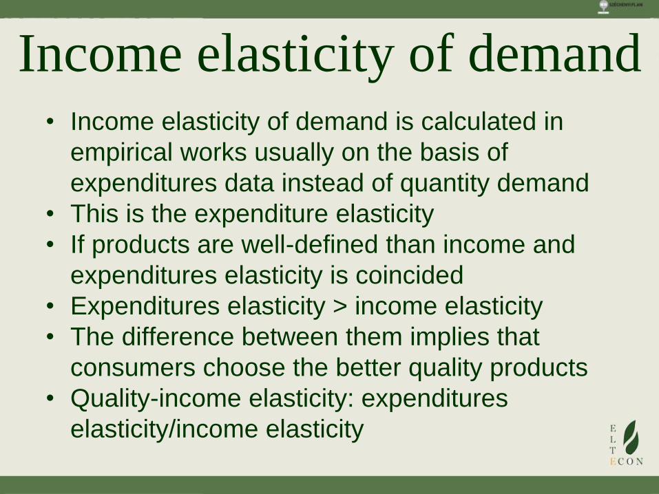
Income elasticity of demand • Income elasticity of demand is calculated in

empirical works usually on the basis of

expenditures data instead of quantity demand

• This is the expenditure elasticity

• If products are well-defined than income and

expenditures elasticity is coincided

• Expenditures elasticity > income elasticity

• The difference between them implies that

consumers choose the better quality products

• Quality-income elasticity: expenditures

elasticity/income elasticity

Relationships between

demand elasticities • Slutsky–Schultz equation:

– Eii+Ei1+Ei2+…+Eiy=0

• Symmetry condition

– Eij=(Rj/Ri)Eji+Rj(Ejy–Eiy)

• Ri share of i product in total expenditures

• Rj share of j product in total expenditures

• Engel equation

– (R1E1y+R2E2y+ …+RnEny)=1

Three types of goods

Impact of income changes

Impact of own

price

Superior

EY>0

Inferior

EY<0

Normal

Ep<0

Normal superior

good: e.g. milk,

butter

Normal inferior

good e.g. milk

powder

Giffen

Ep>0

- Giffen good

Staple foods for

poor people

Approaches of demand analysis • Data:

– Time series

• Aggregate macro data

– Cross-sectional data

• households survey

– Panel data

• Combination of time series and cross-sectional data

• Approaches

– Single equation models

– Total demand system estimations

• Linear expenditure system (LES, Stone, 1954)

• Almost Ideal Demand System (AIDS, Deaton–Muellbauer,

1980)

• Generalized Ideal Demand System (GAIDS, Bollino, 1990)

• Rotterdam model, (Theil, 1976)

• Translog model (Cristensen-Jorgenson-Lau, 1975)

Single equation models

Model Function Elasticity

Linear Y=α+βX β(X/Y)

Log-log logY=α+βlogX β

Log-lin logY=α+βX βX

Lin-log Y=α+βlogX β(1/Y)

Reciprocal Y=α+β(1/X) –β(1/XY)

An example: Hungarian beer

consumption Period: 1980–2004

Number of observations: 25

Variables:

Per capita consumption in l (beer, wine, spirits)

Price in Hungarian Forints (beer, wine, spirits)

Income: per capita GDP

Deflation: price and income data are deflated by CPI

Qbeer=α0+ α1Pbeer+α2Pwine+α3Pspirit+α4Income+ε

We estimate in Log-log function form

Per capita income consumption in l

1980–2004

0

20

40

60

80

100

120

140

160

1980 1982 1984 1986 1988 1990 1992 1994 1996 1998 2000 2002 2004

beer consumption wine consumption spirit consumption

_cons 2.320492 .6965751 3.33 0.003 .8674615 3.773522 ljov .1707309 .0831078 2.05 0.053 -.0026289 .3440908 ltomenyar -.491161 .0993606 -4.94 0.000 -.6984236 -.2838985 lborar .1189198 .0648215 1.83 0.081 -.0162954 .254135 lsorar -.213585 .1892578 -1.13 0.272 -.6083699 .1811999 lsorfogyabs Coef. Std. Err. t P>|t| [95% Conf. Interval]

Total .094967425 24 .003956976 Root MSE = .03609 Adj R-squared = 0.6709 Residual .026046712 20 .001302336 R-squared = 0.7257 Model .068920713 4 .017230178 Prob > F = 0.0000 F( 4, 20) = 13.23 Source SS df MS Number of obs = 25

. reg lsorfogyabs lsorar lborar ltomenyar ljov

Results

Prob > chi2 = 0.7000 chi2(1) = 0.15

Variables: fitted values of lsorfogyabs Ho: Constant varianceBreusch-Pagan / Cook-Weisberg test for heteroskedasticity

Prob > F = 0.0107 F(3, 17) = 5.10 Ho: model has no omitted variablesRamsey RESET test using powers of the fitted values of lsorfogyabs

Durbin-Watson d-statistic( 5, 25) = 1.705783

Slutsky-Schultz

condition is not valid

ΣEij=-0,415

Mean VIF 4.63 ljov 2.72 0.367513 ltomenyar 4.46 0.224437 lsorar 4.52 0.221305 lborar 6.82 0.146635 Variable VIF 1/VIF

Conclusions

• Demand for agricultural products are

usually

– Price inelastic

– Income inelastic

– But, there is a significant differences

across product in terms of price and

income elasticity

– Derived demand