Chapter 5Income and Substitution Effects

Effects of Changes in Income and Prices on Optimum Consumer

Choices

• As shown earlier for utility maximization, x*

(optimal x) is a function of prices and income:

• This chapter deals with this relationship.• These functions can be derived from the constrained

utility maximization problem from the last chapter.• These are demand functions for goods for an

individual consumer! If we know px, py, and I, we can calculate x*, the optimal quantity of x demanded, for a given individual’s utility function.

I),p,p(yy I);,p,x(pxbecomesit goods, For two

1...ni I);,p,...,p,(pxx

yx*

yx*

xxxi*i n21

• Individual demand functions are homogeneous of degree zero in all prices and I. That is, if all prices and income double, x* will not be affected. For example, if I = pxx+pyy, then 2I = 2pxx+2pyy.– On the graph of the budget constraint and will

not change if both numerator and denominator are multiplied by 2 or any other constant (t).

– Preferences do not change, ie., indifference curves do not change with changes in prices or income.

– So if all prices and income move together, no change in x* and y*.

xpI

ypI

yy 2p2I

pI

x

xx 2p2I

pI

x*

y

y*

Pure inflation does not affect choices among goods.

• Changes in Income – Ceteris Paribus Prices and preferences (utility function)

Changes in income shift the budget constraint parallel because prices are assumed not to change.

Successive optima when I changes will have same MRS because the slope of the budget constraint remains the same.

y

1

pI

y

2

pIy

I2 > I1

xx

2

pI

x

1

pI

x* x**

Engel Curves show how x* or y* changes as I changes, Ceteris Paribus.

y

x

*y

*y

*yx

1

pI

x

2

pI

x

3

pI

I3 > I2 > I1 f(I)y*

I or E0

*y

*y

*y

*y

1I 2I 3I

f(I)y*

0

If a line tangent to f(I) at point A has a negative intercept, expenditures on the good (pxx) decrease as a percentage of total expenditures (E) as I increases around point A.

If a line tangent to f(I) at point A has a positive intercept, expenditures on the good (pyy) increase as a percentage of total expenditures (E) as I increases around point A.

*y

I or E

A

Line tangent to f(I) at point A.

If a line tangent to f(I) at point B has a zero intercept, expenditures on the good (pxx) remain constant as a percentage of total expenditures (E) as I increases around point B.

f(I)x*

I or E0

*x

A

Line tangent to f(I) at point A.

B

Line tangent to f(I) at point B.

Normal and Inferior GoodsNormal good 0

Iy*

Luxury, e.g., eating out, boats

Necessity, e.g., underwear

I

y*

Both luxuries and necessities are Normal Goods.

Curves may bend up for luxury goods (fI I > 0) and down for necessities

(fI I < 0).

Mostly we talk about 0.I

y*

y*=f(I)

Inferior good 0I

x *

x*

II0 I1

e.g., macaroni & cheese

Whether a good is normal or inferior may vary along the Engle Curve. The good may change from Normal to Inferior.

I

InferNorm

x0

y

I1

I0

x

I1 > I0

X**

x*X**

X=f(I)

x

• Changes in Prices – Ceteris Paribus. Involves a change in the price ratio (px/py) and thus a change in the slope of the budget constraint and a change in the MRS at the new optimal point, because at optimal, .ppMRS yxxy

y

ypI

0 x

U2

xp

I

S xpI

px decreases to px' causing optimum to

move from A to B (Δx* is total effect).

The total effect is divided into two effects, the substitution effect and the income effect. The substitution effect is the change in x* in going from A to C, while the income effect is the change in x* in going from C to B.

To find C, use the original indifference curve and find the point of tangency with a fictitious budget constraint that has the new price ratio.

What kind of good is x with regard to income? It is a normal good because 0.I

x *

Decrease in nominal income (I) required to stay on same indifference curve.

xx pp

AC

B

U1

InTot

• Summary of substitution and income effects – The movement from A to B is composed of two effects:– Substitution effect - Caused by change in px/py| U = U1.

• Because px is lower, the price ratio is smaller and the new tangency point must be at a smaller MRS (smaller –dy /dx).

• Can measure the substitution effect by holding real income constant (hold U constant), remaining on the same Indifference Curve, but using the new price ratio to find point C. The change in x* in going from A to C measures the substitution effect.

• For a given price change (px), the magnitude of the substitution effect depends on the availability of substitute goods.

Large substitution effect No substitution effect

x

y

x

y

U = U1

U = U0

U = U0

U = U1

– Income Effect – Caused by an increase in real income represented by an increase in utility, or movement to a higher indifference curve. A price decrease brings about an increase in real income; purchasing power. The income effect is the change in x* in going from C to B. The magnitude of the income effect depends on the portion of income spent on x.

• The sum of the Income and Substitution Effects is the total effect of a price change (total change in x*).

• Could show a similar analysis for a price increase (text p. 127).• In most situations, the two effects are complementary, in that they move in

the same direction and reinforce each other as in the case of Normal Goods.

0px

*Ux

*

0

Ix*

For a decrease in px , the substitution effect causes x* to increase holding real income constant (have to reduce nominal income to keep real income constant).

The increase in nominal income required to reach the higher indifference curve (higher real income resulting from the lower price), causes x* to increase further.

Income and Substitution Effects for Inferior Goods• Increasing income causes a decline in purchases of x,

The income effect is perverse for an inferior good.0.

Ix*

BApx Gives Total effect on x*.

BC Gives Income effect 0.I

x *

CA Gives Substitutioneffect 0.

px

1UUx

*

In this case, a decrease in px causes an increase in x*, but only because the substitution effect is large enough to offset the perverse income effect.

y

x

U1

U2CBA

Tot In

S

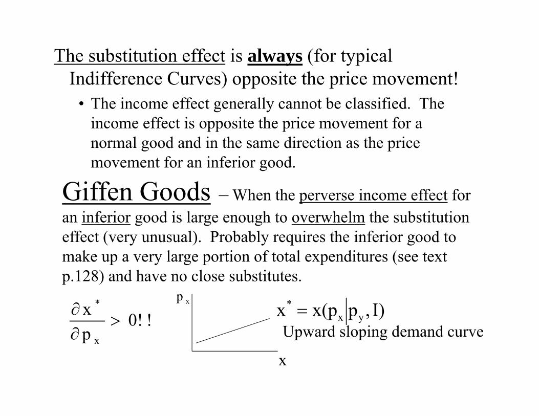
The substitution effect is always (for typical Indifference Curves) opposite the price movement!

• The income effect generally cannot be classified. The income effect is opposite the price movement for a normal good and in the same direction as the price movement for an inferior good.

Giffen Goods – When the perverse income effect for an inferior good is large enough to overwhelm the substitution effect (very unusual). Probably requires the inferior good to make up a very large portion of total expenditures (see text p.128) and have no close substitutes.

!0!px

x

*

Upward sloping demand curve

x

xpI),px(px yx

*

Individual Demand Curve (single consumer)

Demand functions I),p,...,p,(pxxn21 xxx1

*1

from earlier

In a two-good world:Demand functions I),p,x(px yx

* Traditional or Marshallian demand functionsI),p,y(py yx

*

Could hold py, preferences, and I (nominal) constant and vary px to get typical demand curve in px and x space.

px

x

I),px(p yx

I),px(px yx*

I),p,...,p,(pxxn21 xxxn

*n

Shows that successive pricedeclines result in larger optimal quantities of x (except for Giffen goods).

y

Per unit of time

0 x* xpI

*x

xp

I x

xp

I x/unit of time

One person, so indifference curves can’t cross. xxx ppp

px

xp

xp

xp

I),px(px yx

0px

x

*

Shows how x* changes as pxchanges when nominal income (I) and prices of all other goods (py) are constant and when the individual’s preference system constant. This is a Marshallian demand curve (uncompensated demand curve).x/unit of time*x *'x

0x

I),px(p yx

•Shifts in the demand curve are caused by shifts in the individual’s preferences or utility function (shifts in the indifference curves implying changes in the MRS), the prices of other goods, and nominal income.Increase I, the demand curve for x shifts up for normal good (down

for inferior good).Increase py, the demand curve for x shifts up for substitute good

(down for a complement good).Increase MUx relative to MUy, the demand curve for x shifts up.

At any x, MRSxy is larger. The absolute slope of the indifference curve is larger (steeper indifference curve at any level of x).

• Changes in px cause movements along the curve, i.e., “changes in the Quantity Demanded” rather than shifts in demand.

Compensated Demand Curves (Hicksian Demand Curve) – We could eliminate the income effects of changes in px and show the effects on x*, holding utility or real income constant.

xp'xp

y

U1

0

px

)U,pp(x 1yxc

Income compensated demand curve (Hicksian) shows only the substitution effects of changes in px, while py, preferences and utility (real income) are held constant.

Compensated demand curve always has a negative slope because the substitution effect is always negative if MRS is diminishing.

pppp xxxx

Means real income constant!

x/u.t.

x/u.t.

''xp'''

xp

g)diminishin is MRS if always 0p/x( xyxc

Compensated demand curve is steeper (flatter) than the Marshallian demand curve for a normal (inferior) good.

For px > px*, the income effect causes less (more)

consumption for a normal good (an inferior good), so x* decreases more (less) for x than for xc.

For px < px*, the income effect causes more (less) consumption for a normal

good (an inferior good), so x* increases more (less) for x than for xc.

px

Beginning optimal point

x Marshallian

xc Hicksian

X is a normal good on this graph.

px*

*x

px

px

Mathematical Approach to Response to Price Changes

•Income and Substitution Effects (two-good world)•Use the compensated demand function

U),p,(pxx yxc*

real income

and the ordinary demand function.

I),p,x(px yx*

nominal income

“Marshallian”, “Ordinary”, or “Uncompensated”

•These two demand functions are equal at the “beginning point” (U max point) where they cross.

I),p,x(pU),p,(px yxyxc

“Hicksian” or “Compensated”

Next, remember the Expenditure Function U),p,E(pE yx

* Substitute the Expenditure Function into x above and get the following (because I = E at U max).

U)),p,E(p,p,x(pU),p,(px yxyxyxc

xxx

c

pE

Ex

px

px

Partially differentiate with respect to px to getChain rule

xx

c

x pE

Ex

px

px

Rearrange terms to get

We will explore this relationship on next page.

(-) for normal goods (+) for inferior goods

Marshallian (total effect)

Hicksian (sub effect)

This is not the slope of the Marshallian demand curve; it is the inverse of the slope. The more negative ∂x/∂px, the flatter the demand curve. If x were on the vertical axis, this would be the slope of the demand curve.

Always (+ or 0) because a decrease (increase) in pximplies a decrease (increase) in E to maintain same utility level as before the price change. Also, the Expenditure Function is non-decreasing in prices.

xx

c

x pE

Ex

px

px

Income effect

Always (-)(-) except for Giffen good

Usually (+); for normal (+), for inferior (-)

Minus changes sign.

x

c

px

px*

x

x

xc

px

px

xpE

Ex

xpx

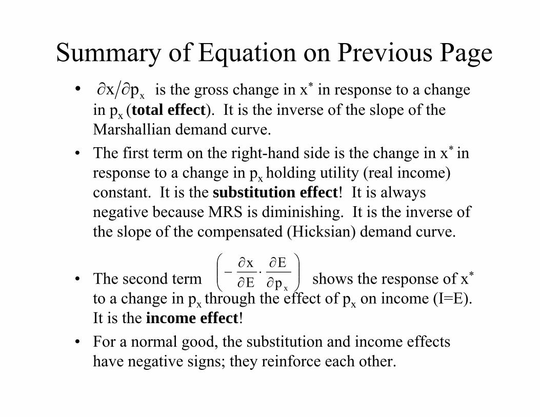
Summary of Equation on Previous Page• is the gross change in x* in response to a change

in px (total effect). It is the inverse of the slope of the Marshallian demand curve.

• The first term on the right-hand side is the change in x* in response to a change in px holding utility (real income) constant. It is the substitution effect! It is always negative because MRS is diminishing. It is the inverse of the slope of the compensated (Hicksian) demand curve.

• The second term shows the response of x*

to a change in px through the effect of px on income (I=E). It is the income effect!

• For a normal good, the substitution and income effects have negative signs; they reinforce each other.

xp

EEx

xpx

The Slutsky Equation

Sub. effect = Uxx

c

px

px

(real income) constant

Inc. effect = xIx

pE

Ix

pE

Ex

xx

Differentiate the expenditure function with respect to px to get xc(px, py,U), which is the compensated demand function. See Shepard’s Lemma and Envelope Theorem on page 137 of text.

E=I

Ixx

px

px

Uxx

The Slutsky Equation – Combine substitution and income effects.

(-) always(-) normal good (+) inferior good

(+) normal good (-) inferior good

(-) always

(-) usually, except Giffen

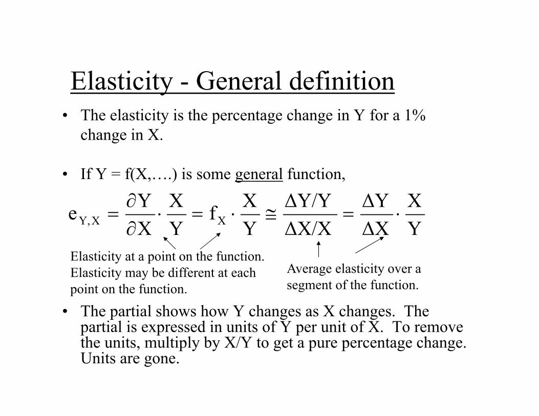
Elasticity - General definition• The elasticity is the percentage change in Y for a 1%

change in X.

• If Y = f(X,….) is some general function,

• The partial shows how Y changes as X changes. The partial is expressed in units of Y per unit of X. To remove the units, multiply by X/Y to get a pure percentage change. Units are gone.

YX

ΔXΔY

ΔX/XΔY/Y

YXf

YX

XYe XXY,

Elasticity at a point on the function. Elasticity may be different at each point on the function.

Average elasticity over a segment of the function.

Marshallian Demand Elasticitiesxp

pxe demand of elasticity Price x

xpx, x

xI

Ixe demand of elasticity Income Ix,

xp

pxe demand of elasticity price-Cross y

ypx, y

The use of partial derivatives indicates that all other demand determinants are held constant.

inelastic 1,e elastic;unit 1,e elastic;1,e Ifxxx px,px,px,

goodinferior ,0e good; normal ,0e If Ix,Ix,

tindependen 0, e

s;complement gross ,0e s;substitute gross ,0e If

y

yy

px,

px,px,

If total expenditures on good x = pxx, then expenditures will react to a price change as follows:

ex,px px px

Elastic (< -1) Exp. Exp.

Unit elastic (= -1) Con. Exp. Con. Exp.

Inelastic (> -1) Exp. Exp.

Because % increase in x is > than % decrease in px.

Because % increase in x is < than % decrease in px.

Effect of a Price Change on Total Expenditures for a Good

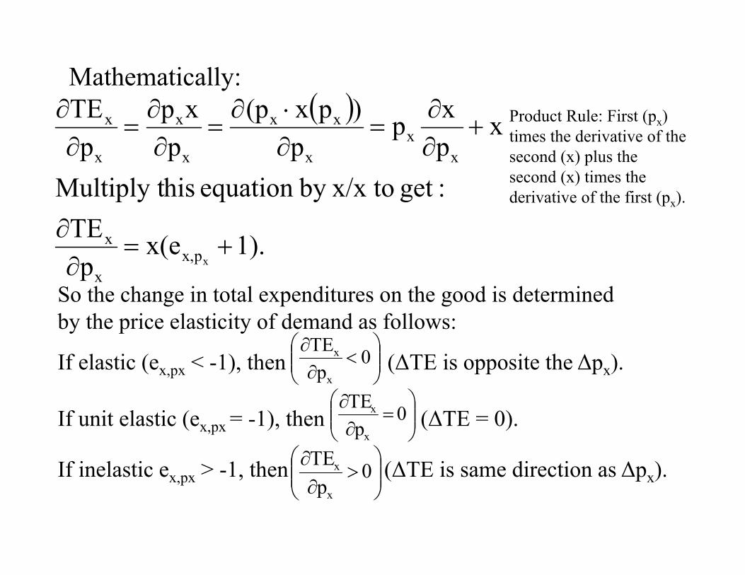
1).x(ep

TE:get x/x toby equation hisMultiply t

xpxp

p)px(p

pxp

pTE

xpx,x

x

xx

x

xx

x

x

x

x

Product Rule: First (px)

times the derivative of the second (x) plus the second (x) times the derivative of the first (px).

If elastic (ex,px < -1), then (ΔTE is opposite the Δpx).

If unit elastic (ex,px = -1), then (ΔTE = 0).

If inelastic ex,px > -1, then (ΔTE is same direction as Δpx).

0

pTE

x

x

0

pTE

x

x

0

pTE

x

x

Mathematically:

So the change in total expenditures on the good is determined by the price elasticity of demand as follows:

Compensated Demand Elasticities

form. elasticityin uationSlutsky Eq theputtingby shown be can

eselasticiti price an Marshalliand eselasticiti price dcompensate thesebetween iprelationsh The

.xp

pxe

:is elasticity price-cross dcompensate theand

xp

pxe:is elasticity

price own dcompensate the thenU),,p,(pxby given is function demand dcompensate theIf

cy

y

cc

px,

cx

x

cc

px,

yxc

y

x

Relationships Among ElasticitiesSlutsky Equation in Elasticity Form

Ixx

px

px

constUxx

Original Slutsky

Multiply by px/x.

x1

Ixxp

px

xp

xp

px

xconstUx

xx

x

xpx,exs Ix,e“Substitution Elasticity”.

The elasticity of the compensated demand curve.

xI

Ix

Ixp

px

xp

xp

px x

constUx

xx

x

Multiply the second term on the right-hand side by I/I.

cpx, y

e

Ix,xc

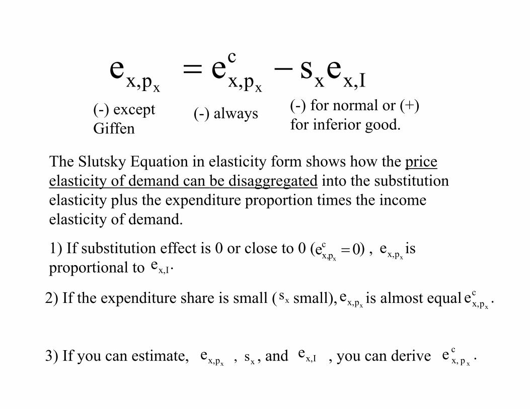
px,px, eseexx

(-) except Giffen

(-) always (-) for normal or (+) for inferior good.

The Slutsky Equation in elasticity form shows how the price elasticity of demand can be disaggregated into the substitution elasticity plus the expenditure proportion times the income elasticity of demand.

1) If substitution effect is 0 or close to 0 ( ) , is proportional to

.e cpx, x

2) If the expenditure share is small ( small), is almost equal

3) If you can estimate, , and , you can derive

.ecpx, x

.e Ix,

xpx,e Ix,e

xpx,e

xs,

0ecpx, x

xpx,e

xs

Euler’s Theorem and the Homogeneity Condition

If is homogeneous of degree m, then

I),p,...,p,f(pxn21 xxx1

.mxI),p,...,p,mf(pIfpf...pfpf 1xxxIxnx2x1n21n21

When m = 0 (because f is homogeneous of degree zero in prices and income), then

0.(0)xIfpf...pfpf 1Ixnx2x1 n21

nxpf

If

Degree of homogeneity (m=0).1xp

f

Homogeneity ConditionBecause demand functions are homogeneous of degree zero, we can use Euler’s theorem on the demand function for x (uncompensated) to get the following for a two-good world:

0IIxp

pxp

px

yy

xx

Dividing through by x gives:

0xI

Ix

xp

px

xp

px y

y

x

x

0eee Ix,px,px, yx

(+) for gross substitutes; (-) for gross complements

(-) except Giffen

(+) for normal good; (-) for inferior good

ConclusionThe sum of own-price, cross-price, and income elasticities equals zero for any specific good. This reaffirms that demand is homogeneous of degree zero (equal percentage changes in prices and income leave the quantity demanded unaffected). If you know or can estimate two of the three terms, you can calculate the third. If you had more than two goods, you would have several cross-price elasticities, some of which could be < 0.

Engel AggregationAssuming a typical consumer (diminishing MRS) and two goods, the budget constraint is:

For utility maximization, an increase in I must be accompanied by an increase in total expenditures because I = E.

The demand functions are:

y.optimallitat Iy*p*xp yx

I),p,y(pyI),p,x(px

yx*

yx*

Differentiate the budget constraint with respect to I assuming optimality:

1I

ypI

xpII *

y

*

x

Multiply the first term on the left-hand side by and multiply the second term by x

I and Ix

.yI and

Iy

1yI

Iy

Iyp

xI

Ix

Ixp yx

Ixpswhere x

x is the proportion of I spent on x and sy is the proportion of I spent on y.

Thus, the proportion of income spent on each good times its income elasticity of demand summed over all goods is 1.

If income increases by 10%, certeris paribus, total purchases must increase by 10% (because of the budget constraint), which implies that goods whose ex,I < 1 must be offset by others whose ex,I > 1 (assumes savings is a good). If you know ex,I and sx and sy in a two-good world, you can calculate ey,I. Engle Aggregation applies to market demand as well as individual demand.

1.es...eses I,xxI,xxI,xx nn2211

1,eses Iy,yIx,x

For n goods

Cournot AggregationThis concept deals with what happens to the demand for all goods when the price of a single good changes.

.seses

:resultCournot thegive toesses0yy

Ip

pyp

Ipx

xx

Ip

pxp0

:get y/y toby last term theand by x/x, first term the/I,pby equation thisof each termMultiply

changes. p when changenot do p and income

nominal because pypx

pxp0

pI

xpy,ypx,x

py,yxpx,x

x

xy

xx

xx

x

xy

xy

xx

x

xx

xx

:get top respect to withconstraintbudget theateDifferentiy.pxpI is constraintbudget The

x

yx

The cross-price effect of a change in px on y demanded is restricted by the budget constraint.

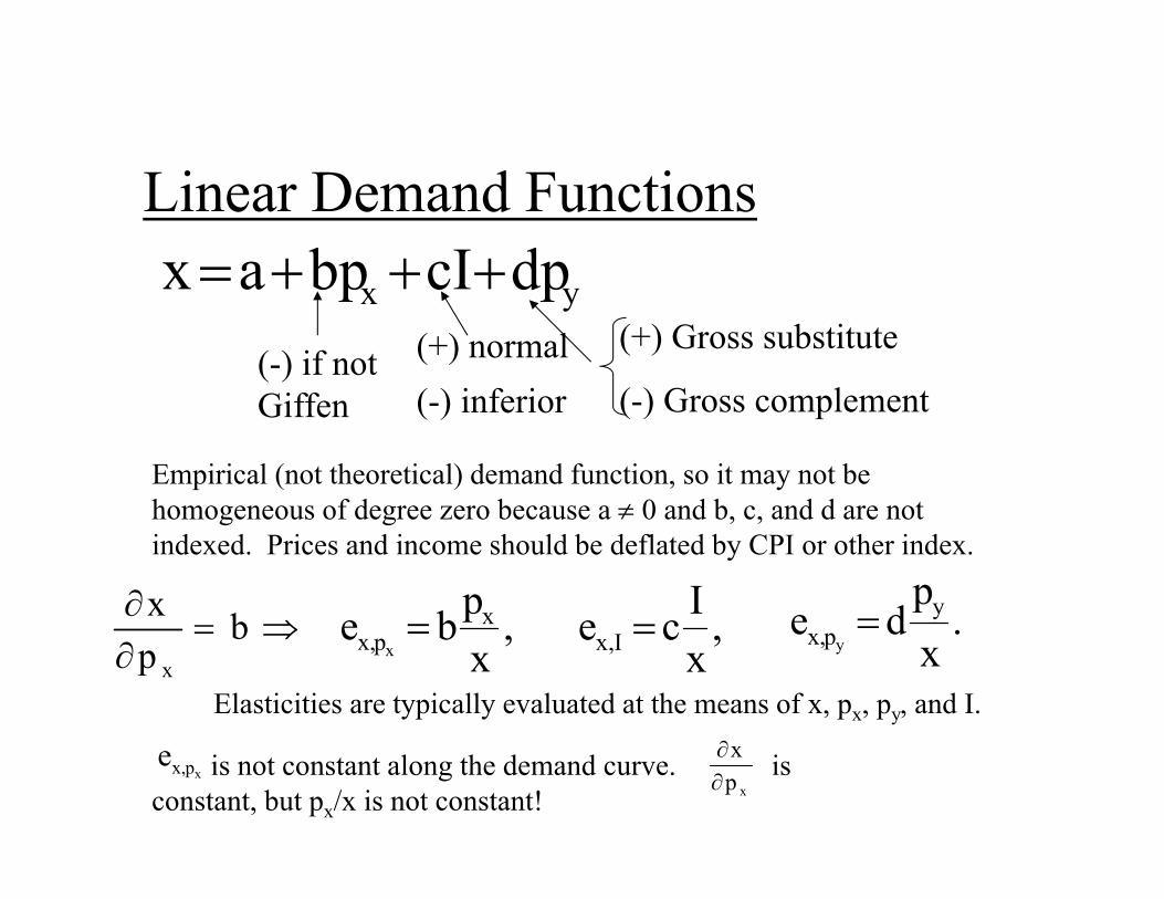
Linear Demand Functionsyx dpcIbpax

Empirical (not theoretical) demand function, so it may not be homogeneous of degree zero because a 0 and b, c, and d are not indexed. Prices and income should be deflated by CPI or other index.

(-) if not Giffen

(+) normal(-) inferior

(+) Gross substitute

(-) Gross complement

bpx

x

,xpbe x

px, x ,

xIce I,x .

xp

de ypx, y

xpx,exp

xis not constant along the demand curve. is

constant, but px/x is not constant!

Elasticities are typically evaluated at the means of x, px, py, and I.

xp

1expx,

1expx,

1expx,

x

=

=

(more negative than –1) Elastic

large

xpx

(between –1 and 0) Inelastic

small

xp x

Constant Elasticity Demand Functionsdy

cbx pIapx

bpIap

ppIabpxp

pxe d

ycb

x

xdy

c1bx

x

xpx, x

Cobb-Douglas type

Or, yx p ln dI ln cp ln ba lnx ln xp

x

So everywhere on the curve. The same property holds for other elasticities (income and cross-price elasticities).

bexpx,

Consumer SurplusUse individual’s x curve --- Consumer surplus is

the area under the x curve, above px

0. It is the amount of extra expenditures an individual would be willing to make above what he/she has to make to get each unit of the good.

“choke price”

market price

CSAppArea Ch

x0x

pxCh

xp

0xp

0 01x x

x

A

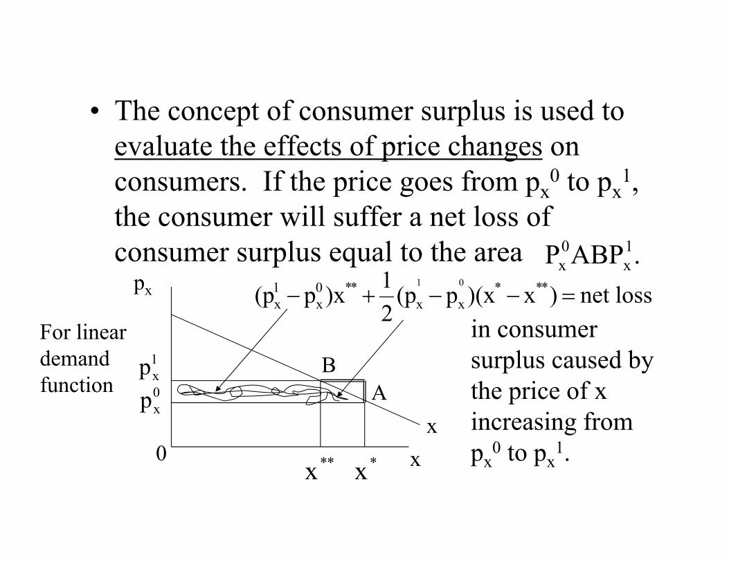
• The concept of consumer surplus is used to evaluate the effects of price changes on consumers. If the price goes from px

0 to px1,

the consumer will suffer a net loss of consumer surplus equal to the area .ABPP 1

x0x

For linear demand function

px

1xp0xp

B

xx

in consumer surplus caused by the price of x increasing from px

0 to px1.

A

lossnet)x)(xp(p21)xp(p ***

xx**0

x1x

01

**x *x0

• We will use the compensated demand curve and the expenditure function to illustrate the measurement of consumer surplus.

• A change in consumer surplus can be measured by expenditure differences to maintain a fixed level of utility, U=U0. Thus we can use the compensated demand function where utility is fixed.

)U,p,E(pE 0y0x0 Expenditures at px

0, given U0 and py.

)U,p,E(pE 0y1x1 Expenditures at px

1 , given U0 and py.

y

1x

ppslope

y

U0

x0EE 10

y

0x

ppslope

0x

1x pp

The change in consumer surplus is E0–E1, which is the negative of the change in expenditures required to maintain the same level of utility when the price changes. For an increase in px, E0–E1<0, meaning real income has fallen and nominal income has to increase to maintain U0. For a decrease in px, E0–E1>0, meaning real income has increased and nominal income has to decrease to maintain U0.

E1 E0

• We can differentiate the expenditure function to get the compensated demand function.

)U,p,(pxxpE

0yxcc

x

As shown earlier by

envelope theorem, “Shephard’s Lemma.”is the change in consumer surplus

for a very small change in px.

The instantaneous change in E resulting from a very small change in px is equal to xc (quantity demanded on the compensated demand curve).

Because the change from px0 to px

1 covers some distance, must integrate to get the change in consumer surplus.

)U,p,(px 0yxc

xpE

Gives the area to left of the compensated demand curve between .pandp 1

x0x

px

1xp0xp

0 1x 0x

xc

x

B

A

x0yx

p

p

c )dpU,p,(pxΔCS1x

0x

CS

• The compensated demand function gives the “true” estimate of the change in consumer surplus resulting from a price change, but it is difficult to estimate, and once estimated, the estimate of consumer surplus is usually quite similar to the estimate obtained from the Marshallian demand curve, so using the Marshallian demand curve is more practical in the real world.