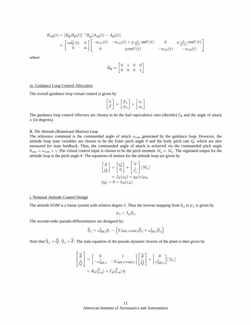
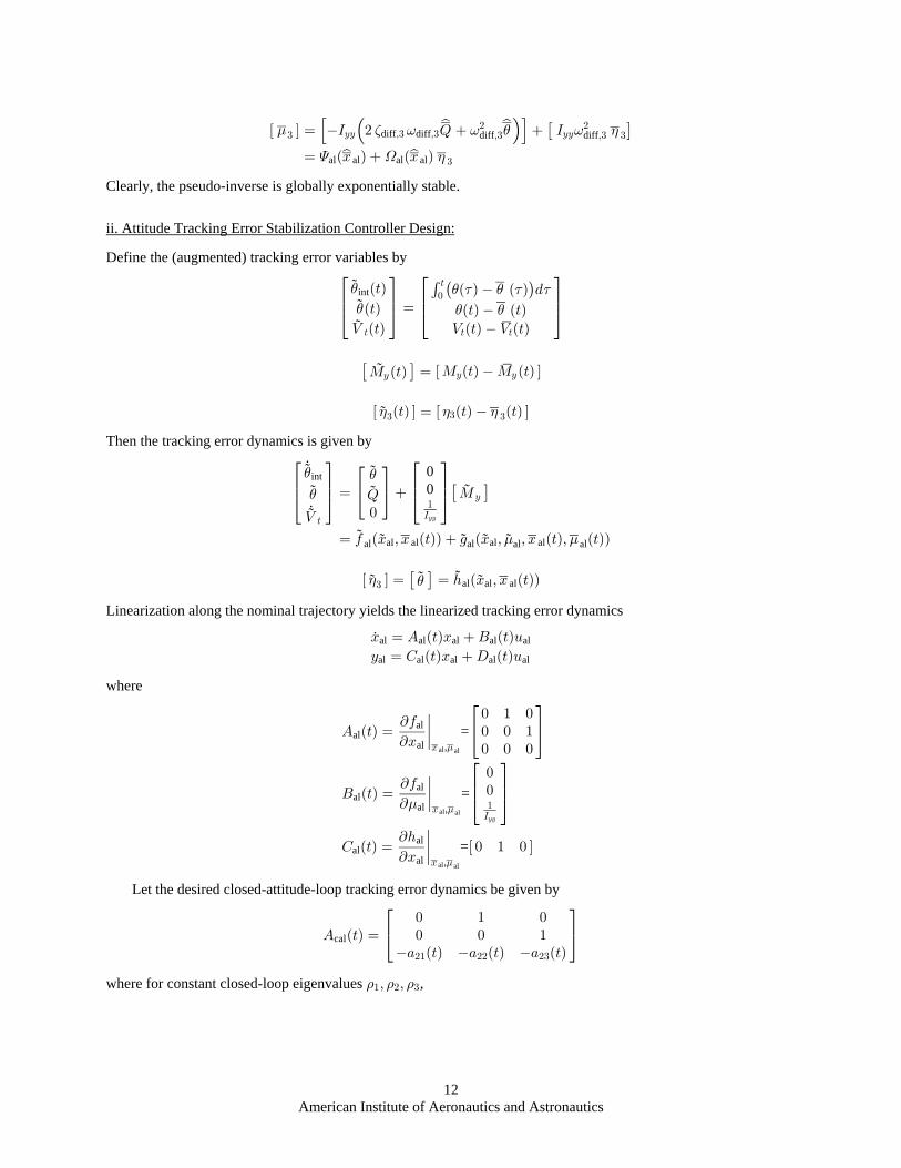
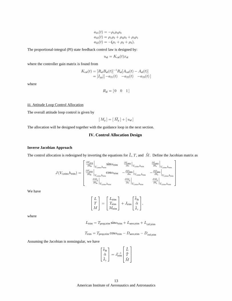
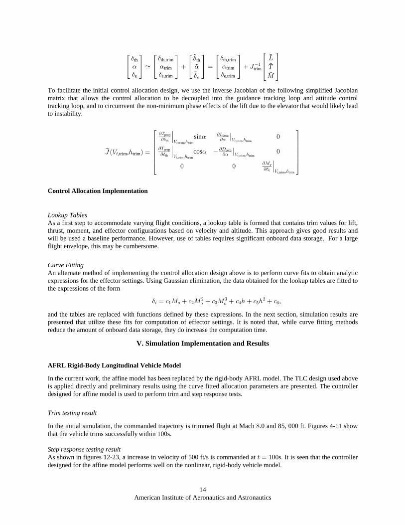
aiaa 2006 gnc final manuscript 080706 rev8

AFRL-VA-WP-TP-2006-330 FLIGHT CONTROL OF HYPERSONIC SCRAMJET VEHICLES USING A DIFFERENTIAL ALGEBRAIC APPROACH (POSTPRINT) Tony A. Adami, J. Jim Zhu, Michael A. Bolender, David B. Doman, and Michael W. Oppenheimer AUGUST 2006

Approved for public release; distribution is unlimited.

STINFO COPY

The U.S. Government is joint author of the work and has the right to use, modify, reproduce, release, perform, display, or disclose the work. AIR VEHICLES DIRECTORATE AIR FORCE MATERIEL COMMAND AIR FORCE RESEARCH LABORATORY WRIGHT-PATTERSON AIR FORCE BASE, OH 45433-7542

NOTICE AND SIGNATURE PAGE

Using Government drawings, specifications, or other data included in this document for any purpose other than Government procurement does not in any way obligate the U.S. Government. The fact that the Government formulated or supplied the drawings, specifications, or other data does not license the holder or any other person or corporation; or convey any rights or permission to manufacture, use, or sell any patented invention that may relate to them. This report was cleared for public release by the Air Force Research Laboratory Wright Site (AFRL/WS) Public Affairs Office and is available to the general public, including foreign nationals. Copies may be obtained from the Defense Technical Information Center (DTIC) (http://www.dtic.mil). AFRL-VA-WP-TP-2006-330 HAS BEEN REVIEWED AND IS APPROVED FOR PUBLICATION IN ACCORDANCE WITH ASSIGNED DISTRIBUTION STATEMENT. *//Signature// //Signature// David B. Doman James H. Myatt Senior Aerospace Engineer Acting Chief Control Design and Analysis Branch Control Design and Analysis Branch Air Force Research Laboratory Air Force Research Laboratory Air Vehicles Directorate Air Vehicles Directorate //Signature// JEFFREY C. TROMP Senior Technical Advisor Control Sciences Division Air Vehicles Directorate This report is published in the interest of scientific and technical information exchange, and its publication does not constitute the Government’s approval or disapproval of its ideas or findings. *Disseminated copies will show “//Signature//” stamped or typed above the signature blocks.

i

REPORT DOCUMENTATION PAGE Form Approved OMB No. 0704-0188

The public reporting burden for this collection of information is estimated to average 1 hour per response, including the time for reviewing instructions, searching existing data sources, searching existing data sources, gathering and maintaining the data needed, and completing and reviewing the collection of information. Send comments regarding this burden estimate or any other aspect of this collection of information, including suggestions for reducing this burden, to Department of Defense, Washington Headquarters Services, Directorate for Information Operations and Reports (0704-0188), 1215 Jefferson Davis Highway, Suite 1204, Arlington, VA 22202-4302. Respondents should be aware that notwithstanding any other provision of law, no person shall be subject to any penalty for failing to comply with a collection of information if it does not display a currently valid OMB control number. PLEASE DO NOT RETURN YOUR FORM TO THE ABOVE ADDRESS.

1. REPORT DATE (DD-MM-YY) 2. REPORT TYPE 3. DATES COVERED (From - To)

August 2006 Conference Paper Postprint 06/15/2005 – 07/31/2006 5a. CONTRACT NUMBER

In-house 5b. GRANT NUMBER

4. TITLE AND SUBTITLE

FLIGHT CONTROL OF HYPERSONIC SCRAMJET VEHICLES USING A DIFFERENTIAL ALGEBRAIC APPROACH (POSTPRINT)

5c. PROGRAM ELEMENT NUMBER 62201F

5d. PROJECT NUMBER

N/A 5e. TASK NUMBER

N/A

6. AUTHOR(S)

Tony A. Adami and J. Jim Zhu (Ohio University) Michael A. Bolender, David B. Doman, and Michael W. Oppenheimer (AFRL/VACA)

5f. WORK UNIT NUMBER

N/A 7. PERFORMING ORGANIZATION NAME(S) AND ADDRESS(ES) 8. PERFORMING ORGANIZATION

REPORT NUMBER

Ohio University Athens, OH 45701

Control Design and Analysis Branch (AFRL/VACA) Control Sciences Division Air Vehicles Directorate Air Force Materiel Command, Air Force Research Laboratory Wright-Patterson Air Force Base, OH 45433-7542

AFRL-VA-WP-TP-2006-330

9. SPONSORING/MONITORING AGENCY NAME(S) AND ADDRESS(ES) 10. SPONSORING/MONITORING AGENCY ACRONYM(S)

AFRL-VA-WP Air Vehicles Directorate Air Force Research Laboratory Air Force Materiel Command Wright-Patterson Air Force Base, OH 45433-7542

11. SPONSORING/MONITORING AGENCY REPORT NUMBER(S)

AFRL-VA-WP-TP-2006-330 12. DISTRIBUTION/AVAILABILITY STATEMENT

Approved for public release; distribution is unlimited. 13. SUPPLEMENTARY NOTES

The U.S. Government is joint author of the work and has the right to use, modify, reproduce, release, perform, display, or disclose the work. Conference paper published in the Proceedings of the AIAA Guidance, Navigation, and Control Conference and Exhibit, published by AIAA. PAO Case Number: AFRL/WS 06-1950 (cleared August 19, 2006).

14. ABSTRACT

Trajectory Linearization Control is applied to the longitudinal hypersonic scramjet vehicle model under development at the Air Force Research Laboratory. The algorithm is based on Differential Algebraic Spectral Theory which features a time-varying eigenvalue concept and avoids the use of so-called frozen-time eigenvalues which can lead to unreliable results when applied to time-varying dynamics systems. A trajectory linearization control was first designed for a non-linear, affine, rigid-body model using an allocation strategy based on trim-condition look-up tables formulated by trimming the model at multiple operating points while varying velocity and altitude. This data was then fitted to a polynomial function, and the lookup tables were replaced by analytical expressions for the effector settings. The TLC design was then verified on the first-principles based, longitudinal, rigid-body hypersonic vehicle model developed at AFRL using both look-up table and curve fit strategies, and simulation testing results are presented. The current design will be further extended to allow adaptive control of time-varying flexible modes using time-varying bandwidth notch filters and a trajectory linearization observer. 15. SUBJECT TERMS

16. SECURITY CLASSIFICATION OF: 19a. NAME OF RESPONSIBLE PERSON (Monitor) a. REPORT Unclassified

b. ABSTRACT Unclassified

c. THIS PAGE Unclassified

17. LIMITATION OF ABSTRACT:

SAR

18. NUMBER OF PAGES

26 David B. Doman 19b. TELEPHONE NUMBER (Include Area Code)

N/A Standard Form 298 (Rev. 8-98)

Prescribed by ANSI Std. Z39-18

1American Institute of Aeronautics and Astronautics

Flight Control of Hypersonic Scramjet Vehicles Using aDifferential Algebraic Approach

Tony A. Adami and J. Jim Zhu* †

Ohio University, Athens, Ohio, 45701

Michael A. Bolender , David B. Doman and Michael Oppenheimer‡ § ¶ ß

Air Force Research Laboratory, Wright Patterson AFB, OH 45433

[Abstract] Trajectory Linearization Control (TLC) is applied to a longitudinalhypersonic scramjet vehicle (HSV) model. The TLC algorithm is based on DifferentialAlgebraic Spectral Theory (DAST) which features a time-varying eigenvalue concept andavoids the use of so-called frozen-time eigenvalues that can lead to unreliable results whenapplied to time-varying dynamical systems. A TLC controller was first designed for anonlinear, affine, rigid-body model using an allocation strategy based on trim-conditionlookup tables. The tables were populated by trimming the model at multiple operatingpoints while varying velocity and altitude. The trim data was then fitted to a cubicpolynomial function, and the lookup tables were replaced by analytical expressions for theeffector settings. The TLC design was then verified on a first-principles based, longitudinal,rigid-body hypersonic vehicle model, and initial simulation testing results are presented.

Nomenclature

B œ State vector. Control vectorœ( Output vectorœ2 œ Altitude# Flight path angleœZ œ> Velocity) Pitch angleœU œ Body pitch rate! Angle of attackœP œ Total liftX œ Total thrustQ œC Pitch MomentP œaero Aerodynamic liftH œaero Aerodynamic dragJ œprop Propulsion forceP œprop Lift due to propulsionH œprop Drag due to propulsionP œctrl Lift due to elevator deflectionH œctrl Drag due to elevator deflectionQ œ9 Mach number$th fuel equivalence ratioœ$/ elevator deflectionœ

* PhD Candidate, Electrical Engineering and Computer Science, Ohio University, Student Member AIAA † Professor, Electrical Engineering and Computer Science, Ohio University, Professional Member AIAA ‡ Aerospace Engineer, Senior Member AIAA § Senior Aerospace Engineer, Associate Fellow AIAA. ¶ Electronics Engineer, Member AIAA


I. Introduction

Hypersonic Scramjet Vehicle (HSV) technology has become attractive in recent years as a possible launch vehiclesolution. Current launch costs (approximately $10,000/lb) are prohibitive, and Scramjet vehicles offer significantrelief by utilizing oxygen in the atmosphere for combustion, thus greatly reducing launch weight. A combined-cycleapproach is eventually envisioned using a vehicle that can alter its propulsion method based on flight conditions.High-speed travel and delivery of cargo (i.e. global overnight delivery) is another potential application for HSV's.

Research and development in this area is currently focusing on several key challenges arising from the uniqueintegration of airframe, propulsion system, and flight control system of HSV's. The supersonic velocities attained bythe air flowing through the combustor dictate a long, slender vehicle fuselage, thus inevitably leading to structuralflexibility. The dependence of the propulsive efficiency on the geometry of the airframe for the ram compressionand external combustion and expansion leads to a coupling between the aerodynamics, structural dynamics and thepropulsion system which must be addressed by the flight control system.

An analytical model based on Newtonian Impact Theory and aero/thermo analysis of the flow in a Scramjet-1-3

type propulsion system has been among the most commonly used for simulation and control design. The dynamicsare strongly influenced by both propulsive and aerodynamic effects, and structural dynamics of the (assumed)elastic vehicle are accounted for using a lump-mass model. Using Lagrangian methods , a model has been obtained%

which captures the dynamics due to the rigid-body, elastic deformation, fluid flow, rotating machinery, wind, and aspherical rotating Earth. Force, moment, and elastic-deformation equations are derived, as well as appropriatekinematic equations. A model based on Compressible Flow Theory is under development that captures the flexible&

structure, aerodynamic, and propulsion system coupling. This model will be described below, and will be used inthis research for control design algorithm development and testing.

Study of the flight dynamics of HSV's has shown that the vehicles are nonlinear, time-varying, coupled,unstable, and non-minimum phase. Furthermore, initial simulations indicated very slow response to a referencecommand. The structural dynamics introduce further complications to the control problem, including modaluncertainty due to coupling effects, potentially time-varying modal frequencies, and the presence of structuralmodes with frequencies within the control bandwidth. Propulsive effects can be essentially viewed as disturbancesto the flight control system. Note that elevator effects constitute an unstable zero dynamics that renders the overallsystem non-minimum phase. If these effects can be canceled using throttle (possible if it produces significant direct‡

lift at or forward of the CG and responds quickly) or by using additional control effectors such as a canard, then theoverall non-minimum phase behavior will be reduced or eliminated.

Flight controller design methods for hypersonic and other elastic vehicles have been an important topic, andinterest continues to grow. A robust control system design has been presented that uses a genetic algorithm to',7

search a design coefficient space. Each search point is evaluated using a Monte Carlo routine that estimates stabilityand performance robustness. Using a 0-1 scale for probability of the vehicle going unstable, the resulting controllerreduced the likelihood of instability from 0.816 to 0.014 compared to open loop operation. Controllers based on themixed-sensitivity technique have been presented that achieve good performance over a large flight envelope.L_

)

The authors address concerns of instability inherent in the technique by ensuring that the frozen operation designpoints are chosen carefully. An output feedback technique using a novel error observer has shown good*

performance in the presence of flexible modes. An examination of the flight dynamics of hypersonic air breathingvehicles reveals the extensive coupling between flight-path and attitude dynamics in the hypersonic region.10

Additionally, this study demonstrates that propulsive performance varies with altitude, Mach number, and angle ofattack. The presence of non-minimum phase characteristics of the lifting body design are addressed by proposing11

an additional control surface. The presence of a canard that is ganged with the elevator can force the right-half planetransmission zero further to the right, allowing for increased freedom in control design in the form of increasedcontroller bandwidth. A pseudo dynamic inversion (DI) controller is proposed that uses an additional feedback12

loop to stabilize the zero dynamics. This avoids the right-half plane pole that DI would introduce in an attempt tocancel the non minimum phase zero. Another DI-based method uses a spline-interpolated lookup table during"$

simulation to calculate the force coefficients, and has shown promising results.In the current research, the authors study the application of Trajectory Linearization Control (TLC) to the1 -1% '

HSV control problem. Nonlinear tracking and decoupling control using TLC is based on Differential AlgebraicSpectral Theory (DAST), and can be viewed as the ideal gain-scheduling controller designed at every point on theflight trajectory. It is an analytical design that provides robustness by design (as opposed to worst-case optimal). Itcombines open-loop and closed-loop control, and is model based, thereby making maximal utilization of known


vehicle properties. In addition, it is adaptive, using time-varying bandwidth (gain) to allow adaptation to modelingerrors and uncertainties, disturbances, control saturations, and failures.

The inherent flexibility of the airframe is an especially vital consideration, and research in this area is veryactive as well. An online adaptive filtering technique that can simultaneously identify multiple modes for flexible17

parameters has been introduced, although results are limited to widely-spaced frequencies. A procedure based ondeeper understanding of acuator dynamics is suggested , and results in a less conservative design.18

This paper describes the HSV models under study in Section II, and provides the theoretical background andpractical application of TLC, including the controller design process for the rigid body HSV longitudinal dynamicsmodel in Section III. A control allocation scheme is discussed in Section IV. Section V describes the currentMatlab/SIMULINK implementation of TLC on the AFRL model, and the trim-testing and step response results arepresented. Section VI concludes the paper with a summary of the main resultsÞ

II. Modeling

A. First-Principles Based Hypersonic Vehicle Model

Researchers at Wright Patterson Air Force Base (WPAFB) in Dayton, OH are developing a generic, hypersonicvehicle longitudinal dynamics model that takes into account structural, aerodynamic, and propulsion systemcoupling.5 Compressible flow theory is used to determine the pressures acting on the vehicle, and oblique shocktheory is used to determine the angle of the bow shock. The forces acting on the airframe are derived in the bodyaxis as and , where the propulsion and aerodynamic forces and moment are heavily coupled and areJ J QB D C

nonlinear functions of the state variables altitude , velocity , angle of attack , and control variables elevator2 Z> !deflection , engine throttle (equivalence fuel ratio) , and the cowl door distance . The model has been$ $e th dBimplemented in MATLAB, and will be treated as a black box.

B. Nonlinear Affine Rigid Body Model for TLC Design

Typical modern nonlinear flight control techniques employ the affine nonlinear state equation model

B œ 0ÐBÑ 1ÐBÑÞ

.

( .œ 2ÐBÑ .ÐBÑ

where is the state vector, is the control vector, and is the output vector. The vector field usually capturesB 0. (inertial and structural couplings, as well as aerodynamic and propulsion couplings of the state variables, while thevector field represents effectiveness of the control effectors on the rate of change of the state variables.1

In order to maximize the crosscutting capability of our design for scaling or alteration of the airframe, ormigration to different airframes, we choose to seperate the inertial/structural dynamics from the aero/propulsivedynamics as

B œ 0 ÐBÑ 0 ÐBÑ 1ÐBÑÞ

" # .

where captures the inertial/structural dynamics due to vehicle mass properties and strucural configuration that0 ÐBÑ"

can be determined by analysis and testing, while represents aerodynamic and propulsive forces and moments0 ÐBÑ2that are usually determined by CFD analysis, wind tunnel testing, and flight data. The control design will first use0 ÐBÑ2 as virtual controls to achieve desired motion, then realize the virtual control commands as a (static) controlallocation design. To this end, and at the present stage, the longitudinal rigid body equations of motion in thestability frame is given by

2 œ ZÞ

> sin#

# #Þœ 1

P "

7 ZŒ cos

>


Z œ 1Þ X

7> sin#

)Þœ U

U œ QÞ "

MCCC

where is the total lift force, is the net thrust force, and is the total pitching moment. These variables will beP X QC

used as virtual controls and are decomposed into componentsP X Qœ ß œ ß œ ß. . ." # $C

P œ P P Paero prop ctrl

X œ H X Haero prop ctrl

Q œ Q QC Cß Cßaero prop

The physical constant parameters are given by:

7 œ $!! 1 œ $#Þ"( V/ œ #Þ!*$ ‚ "! M œ & ‚ "! slug, ft/s , , slug-ft .# ( & #CC

With the state, virtual control input, and output variables defined as given in the nomenclature, the state and outputequations can be written as:

Ô × Ô ×Ö Ù Ö ÙÖ Ù Ö ÙÖ Ù Ö ÙÖ Ù Ö ÙÖ Ù Ö ÙÕ Ø Õ Ø

Ô ×Ö ÙÖ ÙÖ ÙÖ ÙÕ Ø

Ô ×Õ Ø

2Þ

Þ

ZÞ

Þ

UÞ

œ

1

1

!

! ! !

! !

! !

! ! !

! !

œ 0ÐBÑ 1ÐBÑ

#

)

.

>

" " "7

"7

"M

Z

U

PXQ

>

Z Z

C

sincos

sin

#

#

#>

>

CC

Ô × Ô ×Õ Ø Õ Ø

PXQ

Z

C

>œ œ ,Ð ß ß Ñ

P P PX H HQ Q

prop aero ctrl

prop aero ctrl

prop aeroCß Cß

$ !

” • ” •(("

# >œ œ 2ÐBÑ

Z# .

Not that in this simplified case is neither regulated nor measured. However, the altitude will have an effect/ 2on the lift, drag, propulsion, and control forces and moments due to the variations in density and temperature, andwill be included in the design. For autonomous flight, the regulated variables can be the altitude and down rangetrajectories. In that case, flight path angle and velocity become intermediate variables.

C. Nonlinear Affine Virtual Control and Control Effector Model

This study assumes an affine, nonlinear actuator model for virutal control and control effectors in the form of

:ÐBÑ œ : :trim ˜

where is the nominal value of at the trimmed (equilibrium) flight condition , and is the˜: œ :ÐB Ñ : B :trim trim trimperturbation from the nominal which will be approximated by

: œ B`:

`B˜ ˜º

Btrim


where is the perturbation of the flight condition from . The forces and pitch moment are given byB̃ Btrim

P œ G Paero aero,trimP!!̃

H œ G Haero aero,trimH!!̃

P œ G Pctrl ctrl,trimP /$/$̃

H œ G Hctrl ctrl,trimH /$/$̃

J œ G Jprop th prop,trim$th $̃

P œ J J ¶ J Jprop prop prop,trim prop prop,trimtrim trimˆ ‰˜ ˜sin sin sin! ! !

X œ J J ¶ J Jprop prop prop,trim prop prop,trimtrim trimˆ ‰˜ ˜cos cos cos! ! !

Q œ G QC / / C$ $̃ ,trim

Thus

P œ G G G˜ ˜ ˜˜$ >2 P P /$ ! ! $th trimsin! $/

X œ G G G˜ ˜ ˜˜$>2 /$ ! ! $th trimcos H H /! $

Q œ G G GC Q Q Q /˜ ˜ ˜˜$th$ ! $th ! $/

where

P œ P P œ P J P P˜ trim prop,trim trim aero,trim ctrl,trimsin!

X œ X X œ X J H H˜ trim prop,trim trim aero,trim ctrl,trimcos!

Q œ Q QC C˜

Cßtrim

! ! !˜ œ trim

$ $ $˜/ œ e e,trim

$ $ $˜ th th th,trimœ

In this case, the parameters of the model are given by

G Z 2 œ`J

`$ >2 >

Z 2

a b º,trim trimprop

th ,,

$>,trim trim

G Z 2 œ`Q

`Q >

C

Z 2$ th

,trim trim

a b º,trim trimth ,

,$

>


G Z 2 œ`P

`P >

Z 2!a b º,trim trim

aero

,,

!>,trim trim

G Z 2 œ`H

`H >


aero

,,

!>,trim trim

G Z 2 œ`Q

`Q >

C


,,

!>,trim trim

G Z 2 œ`P

`P >

Z 2$/

>

a b º,trim trimaero

e ,,

$,trim trim

G Z 2 œ`H

`H >

Z 2$/

>

a b º,trim trimaero

e ,,

$,trim trim

G Z 2 œ`Q

`Q >

C

Z 2$e

,trim trim

a b º,trim trime ,

,$

>

where the trim values and derivatives are obtained from the AFRL Model by performing a two-dimensionaloptimization at multiple operating points based on velocity and altitude.

III. Trajectory Linearization Controller Design and Simulation Implementation

A. Trajectory Linearization Control (TLC)

TLC provides robust stability and performance without interpolation of controller gains, and eliminates costlycontroller redesigns due to minor airframe alteration. Controller gains for the commanded torque are computedsymbolically based on the theoretical derivations and are applicable to any feasible trajectories and airframes withknown mass properties. Therefore the design is scalable and mission adaptable. Additional features include the useof correct time-varying eigenvalue stability theory, and automated design using symbolic toolbox script. There is nointerpolating for gain-scheduling needed, since the method provides 'ideal' gain-scheduling at every point alongguidance trajectory.

Figure 1 shows a conceptual block diagram of the TLC method. A so-called pseudo-inverse is obtained for thenonlinear plant model to calculate the open-loop nominal control. The tracking error is then driven toward zeroexponentially using a linear time-varying (LTV) tracking error regulator.

Figure 1. Conceptual Configuration Trajectory Linearization Control.


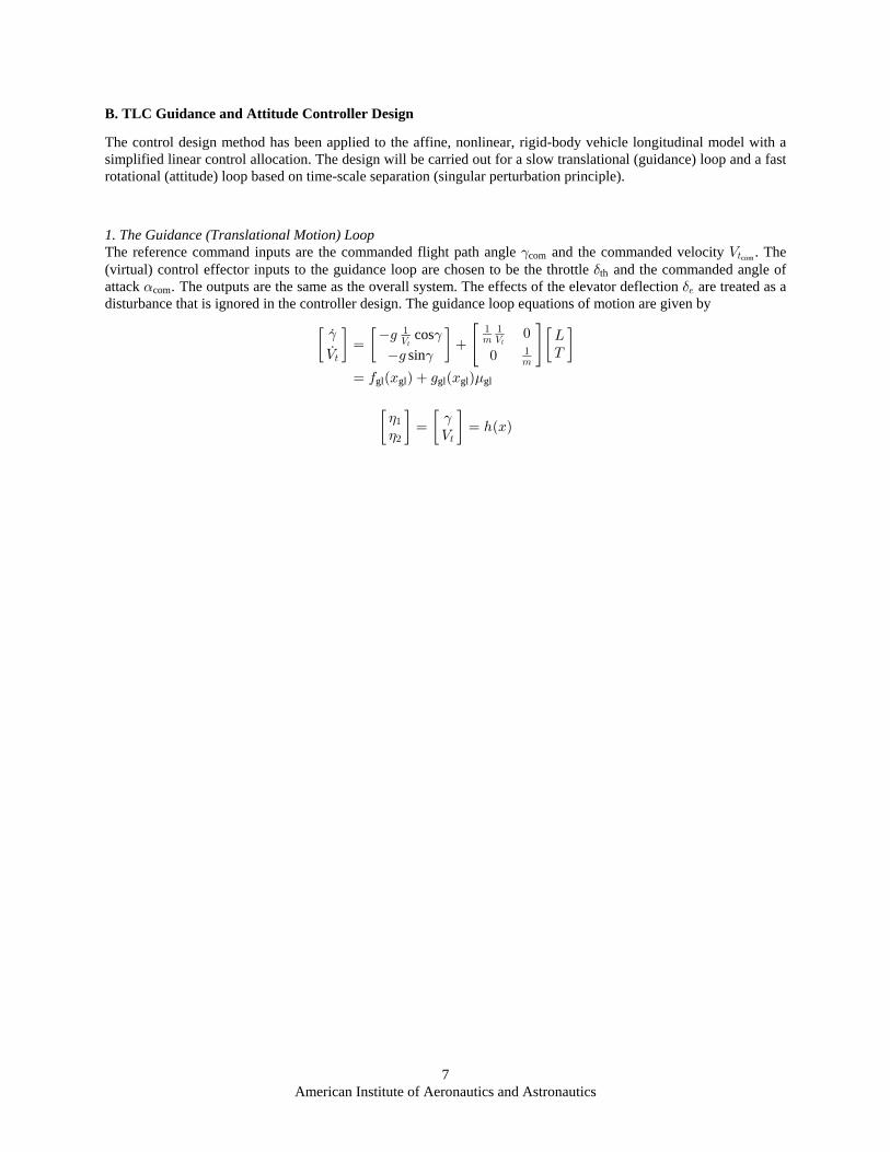
B. TLC Guidance and Attitude Controller Design

The control design method has been applied to the affine, nonlinear, rigid-body vehicle longitudinal model with asimplified linear control allocation. The design will be carried out for a slow translational (guidance) loop and a fastrotational (attitude) loop based on time-scale separation (singular perturbation principle).

1. The Guidance (Translational Motion) LoopThe reference command inputs are the commanded flight path angle and the commanded velocity . The#com Z>com

(virtual) control effector inputs to the guidance loop are chosen to be the throttle and the commanded angle of$thattack . The outputs are the same as the overall system. The effects of the elevator deflection are treated as a! $com /

disturbance that is ignored in the controller design. The guidance loop equations of motion are given by

” • ” • ” •– —#

.

Þ

ZÞ œ

1

1

!

!

œ 0 ÐB Ñ 1 ÐB Ñ

>

" " "7

"7

Z Z> >cos

sin#

#

PX

gl gl gl gl gl

” • ” •(("

# >œ œ 2ÐBÑ

Z#


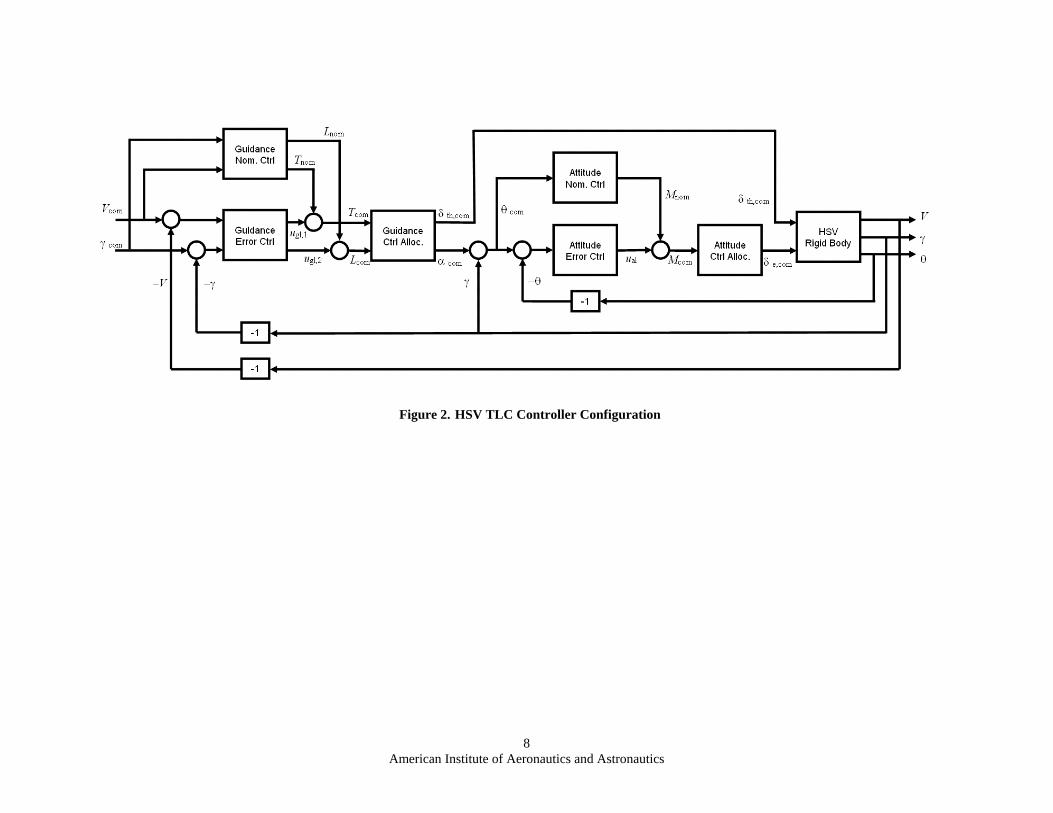
Figure 2. HSV TLC Controller Configuration


i. Nominal Guidance Controller Design:

Since is independent of the input , the relative degree is greater than zero. Taking the time derivative of 2ÐBÑ . (gl "

once yields

( #

(

Þ Þœ œ 1

" " "

7

Þœ Z œ 1

Þ "

7

"

# >

Z ZP

X

> >cos

sin

#

#

Thus the system has a vector relative degree . The inverse mapping from to is given by.

Ò" "Ó ( .gl

P œ 7 U 1 Þ

X œ 7 1 Þ

ˆ ‰a b( #

( #"

#

cossin

The first-order pseudo-differentiators are designed by

( = ( ( s sÞ

œ ß 3 œ "ß #3 3 3ß3diff a bNote that . The state equation of the pseudo dynamic inverse of the plant is then given by( # ( s s sœ ß œ Z

s" >2

– — – — ” •” •# = #

=

== (

(

Q I (

sÞ

ZsÞ œ

s

Zs

œ ÐB Ñ ÐB Ñ s s>

ß" #

ß# >

ß"

ß#

"

#

diff

diff

diff

diff

gl gl gl gl

00

” • ” •Ô ×Ö ÙÕ Ø

Š ‹Š ‹ – —P

X œ

7 Z 1s s s

7 Z 1s s

7Zs

7

œ ÐB Ñ ÐB Ñ s s

> ß"

ß# >

> ß"

ß#

"

#

= # #

= #

==

((

R S (

diff

diff

diff

diff

gl gl gl gl

cos

sin0

0

Clearly, the pseudo-inverse is globally exponentially stable. It is noted that in unaccelerated cruise flight, thenominal thrust . This is because the aerodynamic drag force is not included in the plant model. Rather, it isX œ !

included in the guidance control allocation. Thus, does not mean the throttle . In fact ,X œ ! œ ! œ

$ $ $th th th,trimwhich generates the thrust that cancels out the aerodynamic drag force.

ii. Guidance Tracking Error Stabilization Controller Design:

Define the (augmented) tracking error variables by

Ô ×Ö ÙÖ ÙÕ Ø

Ô ×Ö ÙÖ ÙÖ ÙÕ Ø

' a b' ˆ ‰

##

7 # 7 7

#

7 7 7

˜˜˜˜

int

int

Ð>ÑÐ>Ñ

Z Ð>Ñ

Z Ð>Ñ

œ

Ð Ñ Ð Ñ .

Ð>Ñ Ð>Ñ

Ð Ñ U Ð Ñ .

Ð>Ñ U Ð>Ñ

#

!

>

!

>

#

#

Z

Z>

>

” • ” •PÐ>Ñ Ð>Ñ PÐ>Ñ

X Ð>Ñœ

Ð>Ñ X Ð>Ñ

˜˜

P

X


” • ” •( ( (( ( (˜˜

1 1Ð>Ñ Ð>Ñ Ð>ÑÐ>Ñ Ð>Ñ Ð>Ñ

œ

# #

"

#

Then the tracking error dynamics is given by

Ô × Ô ×Ö Ù Ö ÙÖ Ù Ö ÙÖ Ù Ö ÙÕ Ø Õ Ø

’ “a bc da b

Ô ×Ö ÙÖ ÙÖ ÙÖ ÙÕ Ø

’ “ˆ ‰#

#

#

# #

# # #

˜.

˜.

˜.

˜.

˜˜ +

˜˜ +

0int

˜ +1

˜ +Z

Z

œ 1 Ð>Ñ

Z1 Ð>Ñ Ð>Ñ

P

>

>

#

"UÐ>Ñ

>

7"

Z U

int

0$ >cos

sin sin

˜

0˜

˜ ˜ ˜ ˜ ˜

PÐ>Ñ PÐ>Ñ

X

œ 0 B ß B Ð>Ñ 1 B ß ß B Ð>Ñß Ð>Ñ

"U

7 #1

gl glgl gl gl glgl gla b ˆ ‰. .

” • ” • a b((

#˜˜

˜˜

˜ ˜1gl gl

# >œ œ 2 B ß B Ð>Ñ

Z

Linearization along the nominal trajectory yields the linearized tracking error dynamics

B œ E Ð>ÑB F Ð>Ñ?Þ

C œ G Ð>ÑB H Ð>Ñ?gl gl gl gl gl

gl gl gl gl gl

where

E Ð>Ñ œ`0

`B

! " ! !

! 1 Ð>Ñ ! 1 Ð>Ñ

! ! ! "! 1 Ð>Ñ ! !

F Ð>Ñ œ`0

`

! !

glgl

gl ,

glgl

gl ,

ºÔ ×Ö ÙÖ ÙÖ ÙÕ Ø

ºÔ ×Ö ÙÖ ÙÖ ÙÕ Ø

B

" "UÐ>Ñ

U Ð>Ñ

B

gl gl

gl gl

.

.

=

=

sin cos

cos

# #

#

.

#

" "7 UÐ>Ñ

"7

B

!

! !

!

G Ð>Ñ œ`2

`B

! " ! !! ! ! "gl

gl

gl ,º ” •

gl gl.

=

Let the desired closed-guidance-loop (CGL) tracking error dynamics be given by

E Ð>Ñ œ

! " ! !+ Ð>Ñ + Ð>Ñ ! !

! ! ! "! ! + Ð>Ñ + Ð>Ñ

cgl

Ô ×Ö ÙÖ ÙÕ Ø

""" ""#

"#" "##

where

+ Ð>Ñ œ Ð>Ñ 3 œ "ß #

+ Ð>Ñ œ # Ð>Ñ Þ

Ð>Ñ

Ð>Ñ

"3" "3#

"3# "3 "3"3

"3

=

' ==

=

Design a proportional-integral (PI) state feedback control law

? œ O Ð>ÑB

œ O Ð>Ñ O Ð>ÑB BB B

gl cgl gl

P,cgl I,cgl2

4” • ” •"

$

where the controller gain matrix is found from


O Ð>Ñ œ ÒV F Ð>ÑÓ V E Ð>Ñ E Ð>Ñ

œ7U Ð>Ñ !

! 7

+ Ð>Ñ + Ð>Ñ 1 Ð>Ñ ! 1 Ð>Ñ

! 1 Ð>Ñ + Ð>Ñ + Ð>

cgl gl gl cgl glgl"

""" ""#" "

UÐ>Ñ

U Ð>Ñ

"#" "##

c d” •– —sin cos

cos

# #

#

#

Ñ

where

V œ! " ! !! ! ! "gl ” •

iii. Guidance Loop Control Allocation

The overall guidance loop virtual control is given by

” • ” • ” •PX

œ

??

.

.1

#

"

#

The guidance loop control effectors are chosen to be the fuel equivalence ratio (throttle) and the angle of attack$th! (in degrees).

B. The Attitude (Rotational Motion) LoopThe reference command is the commanded angle of attack generated by the guidance loop. However, the!comattitude loop state variables are chosen to be the Euler pitch angle and the body pitch rate , which are also) Umeasured for state feedback. Thus, the commanded angle of attack is achieved via the commanded pitch angle) !com comœ Þ Q œ# The virtual control input is chosen to be the pitch moment . The regulated output for theC QC

attitude loop is the pitch angle . The equations of motion for the attitude loop are given by)

” • ” • – —c d)

.

(

Þ

UÞ œ

!

!

œ 0 ÐB Ñ 1 ÐBÑ

Ò Ó œ œ 2 ÐB Ñ

UQ"

M

$

CC

C

al al al al

al al)

i. Nominal Attitude Control Design

The attitude EOM is a linear system with relative degree . Thus the inverse mapping from to is given by.

# ( .$ $

. ( œ MÞÞ

$ $CC

The second-order pseudo-differentiators are designed by:

( = ( ' = ( = ( s s sÞÞ Þ

œ # $ 3 $ $ß$ ß$# #

ß$ ß$diff diffdiff diffŠ ‹Note that . The state equation of the pseudo dynamic inverse of the plant is then given by( ( ) s s

Þœ Uß œ

s s$ $

Ô ×Õ Ø ” • ” •– — c d) )

= ' = =(

Q 0 I 0 (

s sÞ

UsÞ œ

! "

# Us

œ Ð Ñ Ð Ñ s s

diff diffdiff diff

al alal al

ß$ ß$# #

ß$ ß$$

0


c d ’ “Š ‹ ‘. ' = = ) = (

R S (

œ M # U M s s

œ ÐB Ñ ÐB Ñ s s

$ CC ß$ ß$ CCß$ ß$# #

$

$

diff diff diff diff

al al al al

Clearly, the pseudo-inverse is globally exponentially stable.

ii. Attitude Tracking Error Stabilization Controller Design:

Define the (augmented) tracking error variables by

Ô × Ô ×Ö Ù Ö ÙÕ Ø Õ Ø

' ˆ ‰)

)

7 ) 7 7

)

˜˜˜

intÐ>Ñ

Ð>Ñ

Z Ð>Ñ

œÐ Ñ Ð Ñ .

Ð>Ñ Ð>Ñ

Ð>Ñ Z Ð>Ñ

>

!

>

>

)

)

Z>

‘ c dQ Q QC C C˜ Ð>Ñ œ Ð>Ñ Ð>Ñ

c d c d( ( (˜$ $$Ð>Ñ Ð>Ñ Ð>Ñœ

Then the tracking error dynamics is given by

Ô × Ô ×Ö Ù Ö ÙÕ Ø Õ Ø

Ô ×Õ Ø ‘

a b a b

)

)

)

. .

˜.

˜˜.

˜˜

00 ˜

˜ ˜ ˜ ˜ ˜

int

al alal al al alal al

Z

œ U!

Q

œ 0 B ß B Ð>Ñ 1 B ß ß B Ð>Ñß Ð>Ñ >

"M

C

CC

c d a b ‘( )˜ ˜ ˜ ˜$ œ œ 2 B ß B Ð>Ñal al al

Linearization along the nominal trajectory yields the linearized tracking error dynamics

B œ E Ð>ÑB F Ð>Ñ?Þ

C œ G Ð>ÑB H Ð>Ñ?al al al al al

al al al al al

where

E Ð>Ñ œ`0

`B

! " !! ! "! ! !

F Ð>Ñ œ`0

`

!!

G Ð>Ñ œ`2

`B! " !

alal

al ,

alal

al ,

alal

al ,

º Ô ×Õ Ø

º Ô ×Ö ÙÕ Ø

º c d

B

B "M

B

al al

al al

al al

.

.

.

=

=

=

.CC

Let the desired closed-attitude-loop tracking error dynamics be given by

E Ð>Ñ œ! " !! ! "

+ Ð>Ñ + Ð>Ñ + Ð>Ñcal

Ô ×Õ Ø

#" ## #$

where for constant closed-loop eigenvalues ,3 3 3" # $ß ß


+ Ð>Ñ œ

+ Ð>Ñ œ

+ Ð>Ñ œ Ñ

#" " # $

## " # # $ $ "

## " # $

3 3 3

3 3 3 3 3 3

3 3 3( .

The proportional-integral (PI) state feedback control law is designed by:

? œ O Ð>ÑBal cal al

where the controller gain matrix is found from

O Ð>Ñ œ ÒV F Ð>ÑÓ V E Ð>Ñ E Ð>Ñ

œ ÒM Ó + Ð>Ñ + Ð>Ñ + Ð>Ñcal al al al cal al

"

CC #" ## #$

c dc dwhere

V œ ! ! "al c diii. Attitude Loop Control Allocation

The overall attitude loop control is given by

c d c d c dQ QC Cœ

?al

The allocation will be designed together with the guidance loop in the next section.

IV. Control Allocation Design

Inverse Jacobian Approach

The control allocation is redesigned by inverting the equations for , , and . Define the Jacobian matrix as˜ ˜P X Q

N Z 2 œa bÔ ×Ö ÙÖ ÙÖ ÙÖ ÙÖ ÙÕ Ø

¹ ¹¸¹>

`J

` ` `Z 2 Z 2

`P `PZ 2

`J

` Z,trim trim

, ,trim ,

,,

prop

th e,trim trim ,trim trim

aero aero

,trim trim

prop

th,trim

$ ! $

$

> >>

>

sin!

2 Z 2

`H `H` `Z 2

`Q `Q `Q` ` `Z 2 Z 2 Z 2

trim ,trim trim

aero aero

,trim trim e

th e,trim trim ,trim trim ,trim trim

cos!trim , ,

, , ,

¸ ¹¹ ¹ ¹

! $

$ ! $

>>

C C C

> > >

We have

Ô × Ô × Ô ×Õ Ø Õ Ø Õ Ø

P PX XQ Q

œ Ntrim th

trim

trim

trim

$!

$

˜˜˜

./

where

P œ X P Ptrim prop,trim trim aero,trim ctrl,trimsin!

X œ X H Htrim prop,trim trim aero,trim ctrl,trimcos!

Assuming the Jacobian is nonsingular, we have

Ô ×Õ Ø

Ô ×Ö ÙÕ Ø

$!

$

˜˜˜

˜˜˜

th

trim

/

"œ N

P

X

Q


Ô × Ô × Ô × Ô ×Õ Ø Õ Ø Õ Ø Õ Ø

Ô ×Ö ÙÕ Ø

$ $! ! ! !$ $ $

$ $

$

th th

e e,trim e,trim

th,trim th,trim

trim trim trim¶ œ N

P

X

Q

˜˜˜

˜˜˜/

"

To facilitate the initial control allocation design, we use the inverse Jacobian of the following simplified Jacobianmatrix that allows the control allocation to be decoupled into the guidance tracking loop and attitude controltracking loop, and to circumvent the non-minimum phase effects of the lift due to the elevator that would likely leadto instability.

N Z 2 œs

!

a bÔ ×Ö ÙÖ ÙÖ ÙÖ ÙÖ ÙÕ Ø

¹ ¸¹ ¸

>

`X

` `Z 2

`PZ 2

`X

` `Z 2

`HZ,trim trim

, ,

,,

prop

th,trim trim

aero

,trim trim

prop

th,trim trim

aero

,trim

$ !

$ !

>>

>>

sin

cos

!

! ,

,

2

`Q` Z 2

trim

e,trim trim

!

! ! ¹C

>$

Control Allocation Implementation

Lookup TablesAs a first step to accommodate varying flight conditions, a lookup table is formed that contains trim values for lift,thrust, moment, and effector configurations based on velocity and altitude. This approach gives good results andwill be used a baseline performance. However, use of tables requires significant onboard data storage. For a largeflight envelope, this may be cumbersome.

Curve FittingAn alternate method of implementing the control allocation design above is to perform curve fits to obtain analyticexpressions for the effector settings. Using Gaussian elimination, the data obtained for the lookup tables are fitted tothe expressions of the form

$3 " 9 # $ % & '9 9# $ #œ - Q - Q - Q - 2 - 2 - ,

and the tables are replaced with functions defined by these expressions. In the next section, simulation results arepresented that utilize these fits for computation of effector settings. It is noted that, while curve fitting methodsreduce the amount of onboard data storage, they do increase the computation time.

V. Simulation Implementation and Results

AFRL Rigid-Body Longitudinal Vehicle Model

In the current work, the affine model has been replaced by the rigid-body AFRL model. The TLC design used aboveis applied directly and preliminary results using the curve fitted allocation parameters are presented. The controllerdesigned for affine model is used to perform trim and step response tests.

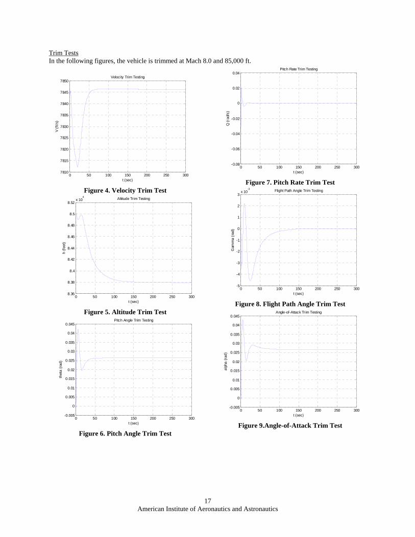
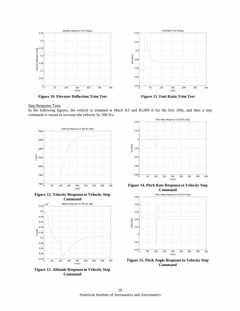
Trim testing result

In the initial simulation, the commanded trajectory is trimmed flight at Mach .0 and 85, 000 ft. Figures 4-11 show)that the vehicle trims successfully within 100s.

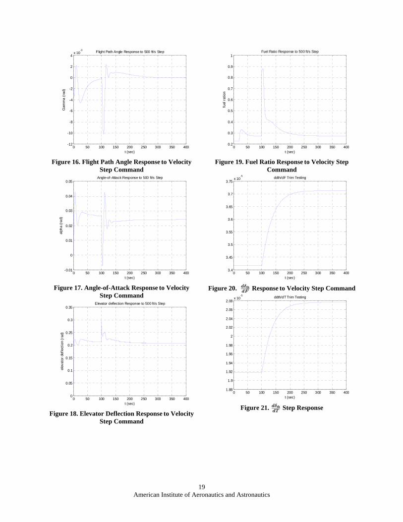
Step response testing resultAs shown in figures 12-23, a increase in velocity of 500 ft/s is commanded at 0 s. It is seen that the controller> œ " !designed for the affine model performs well on the nonlinear, rigid-body vehicle model.


VI. ConclusionInitial study of the longitudinal hypersonic scramjet vehicle model under development at AFRL has revealed a richbut complex control design problem. The tight integration of propulsion and airframe presents unique challenges,and makes addressing the structural dynamics of the vehicle a critical issue. In the paper, a TLC design is presentedand verified with successful trim and step response simulation on the rigid-body, longitudinal AFRL HSV model.Current work addresses the rigid body AFRL model directly, and a comparison is drawn between allocationschemes bases on lookup tables and fitted expressions. Initial simulation results are presented and show a stablecontroller that can fly trim flights as well as perform basic maneuvers.

VI. AcknowledgementsThe Ohio University authors would like to thank the Dayton Area Graduate Studies Institude for providing fundingfor this project.


Theta_out

Q_out

Gamma_out

V_out

Signal Generator

h_nom

Mu_nom

V_nom

GuideNomCtrl

V_nom

h_nom

L_com

T_com

alphaalpha_com

GuideAlloc

Guidance ErrorControl

m

Gain7

-1

Gain5

-1

Gain4

-1

Gain3

-1

Gain2

-1

Gain1

-1

Gain

[Gam_nom]

From1

[V_nom]

From

f(u)

Fcn

.6

Constant2

ThetaCom

Mnom

X_nom

AttNomCtrl

AttErrCtrl

Att Error Ctrl

V_nom

h_nom de

Att CtrlAllocation

In1

In2

In3

Vt

alpha

Q

theta

AFRL ModelThr_nom

L_nom

V_nom

V_com

Gamma_com

Thr_ctrl

L_ctrlL_com

T_com

h_nom

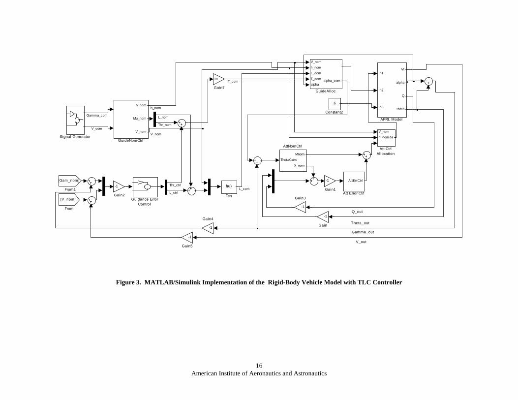
Figure 3. MATLAB/Simulink Implementation of the Rigid-Body Vehicle Model with TLC Controller


Trim TestsIn the following figures, the vehicle is trimmed at Mach 8.0 and 85,000 ft.

0 50 100 150 200 250 3007810

7815

7820

7825

7830

7835

7840

7845

7850

t (sec)

V (ft

/s)

Velocity Trim Testing

Figure 4. Velocity Trim Test

0 50 100 150 200 250 3008.36

8.38

8.4

8.42

8.44

8.46

8.48

8.5

8.52x 10

4

t (sec)

h (fe

et)

Altitude Trim Testing

Figure 5. Altitude Trim Test

0 50 100 150 200 250 300-0.005

0

0.005

0.01

0.015

0.02

0.025

0.03

0.035

0.04

0.045

t (sec)

thet

a (ra

d)

Pitch Angle Trim Testing

Figure 6. Pitch Angle Trim Test

0 50 100 150 200 250 300-0.08

-0.06

-0.04

-0.02

0

0.02

0.04

t (sec)

Q (r

ad/s

)

Pitch Rate Trim Testing

Figure 7. Pitch Rate Trim Test

0 50 100 150 200 250 300-5

-4

-3

-2

-1

0

1

2

3x 10

-3

t (sec)

Gam

ma

(rad

)

Flight Path Angle Trim Testing

Figure 8. Flight Path Angle Trim Test

0 50 100 150 200 250 300-0.005

0

0.005

0.01

0.015

0.02

0.025

0.03

0.035

0.04

0.045

t (sec)

alph

a (ra

d)

Angle-of-Attack Trim Testing

Figure 9.Angle-of-Attack Trim Test


0 50 100 150 200 250 3000

0.05

0.1

0.15

0.2

0.25

0.3

0.35

t (sec)

elev

ator

def

lect

ion

(rad

)

Elevator deflection Trim Testing

Figure 10. Elevator Deflection Trim Test

0 50 100 150 200 250 3000.22

0.24

0.26

0.28

0.3

0.32

0.34

t (sec)

fuel

ratio

n

Fuel Ratio Trim Testing

Figure 11. Fuel Ratio Trim Test

Step Response TestsIn the following figures, the vehicle is trimmed at Mach 8.0 and 85,000 ft for the first 100s, and then a stepcommand is issued to increase the velocity by 500 ft/s.

0 50 100 150 200 250 300 350 4007800

7900

8000

8100

8200

8300

8400

t (sec)

V (ft

/s)

Velocity Response to 500 ft/s Step

Figure 12. Velocity Response to Velocity StepCommand

0 50 100 150 200 250 300 350 4008.32

8.34

8.36

8.38

8.4

8.42

8.44

8.46

8.48

8.5

8.52x 10

4

t (sec)

h (fe

et)

Altitude Response to 500 ft/s Step

Figure 13. Altitude Response to Velocity StepCommand

0 50 100 150 200 250 300 350 400-0.08

-0.06

-0.04

-0.02

0

0.02

0.04

t (sec)

Q (r

ad/s

)

Pitch Rate Response to 500 ft/s Step

Figure 14. Pitch Rate Response to Velocity StepCommand

0 50 100 150 200 250 300 350 400-0.02

-0.01

0

0.01

0.02

0.03

0.04

0.05

t (sec)

thet

a (ra

d)

Pitch Angle Response to 500 ft/s Step

Figure 15. Pitch Angle Response to Velocity StepCommand


0 50 100 150 200 250 300 350 400-12

-10

-8

-6

-4

-2

0

2

4x 10

-3

t (sec)

Gam

ma

(rad

)

Flight Path Angle Response to 500 ft/s Step

Figure 16. Flight Path Angle Response to VelocityStep Command

0 50 100 150 200 250 300 350 400-0.01

0

0.01

0.02

0.03

0.04

0.05

t (sec)

alph

a (ra

d)

Angle-of-Attack Response to 500 ft/s Step

Figure 17. Angle-of-Attack Response to VelocityStep Command

0 50 100 150 200 250 300 350 4000

0.05

0.1

0.15

0.2

0.25

0.3

0.35

t (sec)

elev

ator

def

lect

ion

(rad

)

Elevator deflection Response to 500 ft/s Step

Figure 18. Elevator Deflection Response to VelocityStep Command

0 50 100 150 200 250 300 350 4000.2

0.3

0.4

0.5

0.6

0.7

0.8

0.9

1

t (sec)

fuel

ratio

n

Fuel Ratio Response to 500 ft/s Step

Figure 19. Fuel Ratio Response to Velocity StepCommand

0 50 100 150 200 250 300 350 4003.4

3.45

3.5

3.55

3.6

3.65

3.7

3.75x 10

-5

t (sec)

ddth/dF Trim Testing

Figure 20. Response to Velocity Step Command..J$th

0 50 100 150 200 250 300 350 4001.88

1.9

1.92

1.94

1.96

1.98

2

2.02

2.04

2.06

2.08x 10

-5

t (sec)

ddth/dT Trim Testing

Figure 21. Step Response..X$th


0 50 100 150 200 250 300 350 4002.15

2.2

2.25

2.3

2.35

2.4x 10

-4

t (sec)

dalpha/dL Trim Testing

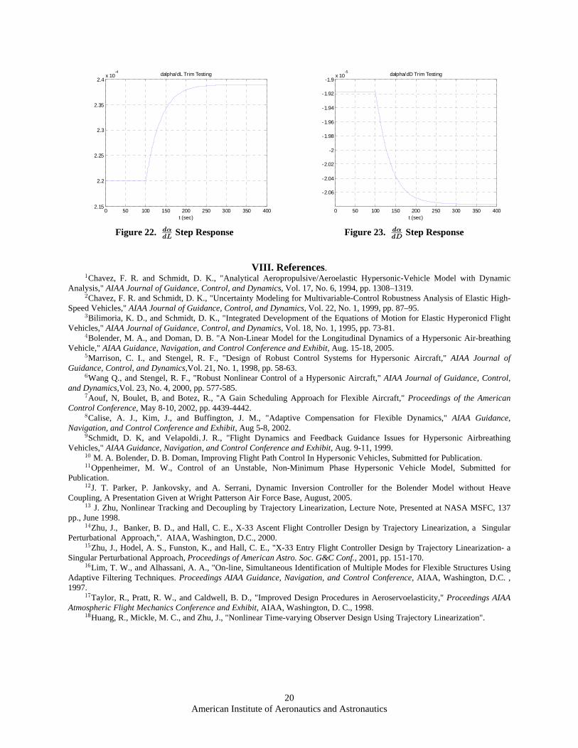
Figure 22. Step Response..P!

0 50 100 150 200 250 300 350 400

-2.06

-2.04

-2.02

-2

-1.98

-1.96

-1.94

-1.92

-1.9x 10

-5

t (sec)

dalpha/dD Trim Testing

Figure 23. Step Response..H!

VIII. References."Chavez, F. R. and Schmidt, D. K., "Analytical Aeropropulsive/Aeroelastic Hypersonic-Vehicle Model with Dynamic

Analysis," , Vol. 17, No. 6, 1994, pp. 1308–1319.AIAA Journal of Guidance, Control, and Dynamics#Chavez, F. R. and Schmidt, D. K., "Uncertainty Modeling for Multivariable-Control Robustness Analysis of Elastic High-

Speed Vehicles," 22, No. 1, 1999, pp. 87–95.AIAA Journal of Guidance, Control, and Dynamics, Vol.$Bilimoria, K. D., and Schmidt, D. K., "Integrated Development of the Equations of Motion for Elastic Hyperonicd Flight

Vehicles," Vol. 18, No. 1, 1995, pp. 73-81.AIAA Journal of Guidance, Control, and Dynamics,%Bolender, M. A., and Doman, D. B. "A Non-Linear Model for the Longitudinal Dynamics of a Hypersonic Air-breathing

Vehicle," Aug. 15-18, 2005.AIAA Guidance, Navigation, and Control Conference and Exhibit,&Marrison, C. I., and Stengel, R. F., "Design of Robust Control Systems for Hypersonic Aircraft," AIAA Journal of

Guidance, Control, and Dynamics,Vol. 21, No. 1, 1998, pp. 58-63.'Wang Q., and Stengel, R. F., "Robust Nonlinear Control of a Hypersonic Aircraft," AIAA Journal of Guidance, Control,

and Dynamics,Vol. 23, No. 4, 2000, pp. 577-585.(Aouf, N, Boulet, B, and Botez, R., "A Gain Scheduling Approach for Flexible Aircraft," Proceedings of the American

Control Conference, May 8-10, 2002, pp. 4439-4442.)Calise, A. J., Kim, J., and Buffington, J. M., "Adaptive Compensation for Flexible Dynamics," AIAA Guidance,

Navigation, and Control Conference and Exhibit, Aug 5-8, 2002.*Schmidt, D. K, and Velapoldi J. R., "Flight Dynamics and Feedback Guidance Issues for Hypersonic Airbreathingß

Vehicles," Aug. 9-11, 1999.AIAA Guidance, Navigation, and Control Conference and Exhibit,"! M. A. Bolender, D. B. Doman, Improving Flight Path Control In Hypersonic Vehicles, Submitted for Publication.""Oppenheimer, M. W., Control of an Unstable, Non-Minimum Phase Hypersonic Vehicle Model, Submitted for

Publication."#J. T. Parker, P. Jankovsky, and A. Serrani, Dynamic Inversion Controller for the Bolender Model without Heave

Coupling, A Presentation Given at Wright Patterson Air Force Base, August, 2005."$ J. Zhu, Nonlinear Tracking and Decoupling by Trajectory Linearization, Lecture Note, Presented at NASA MSFC, 137

pp., June 1998."%Zhu, J., Banker, B. D., and Hall, C. E., X-33 Ascent Flight Controller Design by Trajectory Linearization, a Singular

Perturbational Approach,". AIAA, Washington, D.C., 2000."&Zhu, J., Hodel, A. S., Funston, K., and Hall, C. E., "X-33 Entry Flight Controller Design by Trajectory Linearization- a

Singular Perturbational Approach, pp. 151-170.Proceedings of American Astro. Soc. G&C Conf., 2001,"'Lim, T. W., and Alhassani, A. A., "On-line, Simultaneous Identification of Multiple Modes for Flexible Structures Using

Adaptive Filtering Techniques. AIAA, Washington, D.C. ,Proceedings AIAA Guidance, Navigation, and Control Conference,1997.

"(Taylor, R., Pratt, R. W., and Caldwell, B. D., "Improved Design Procedures in Aeroservoelasticity," Proceedings AIAAAtmospheric Flight Mechanics Conference and Exhibit, AIAA, Washington, D. C., 1998.

"8Huang, R., Mickle, M. C., and Zhu, J., "Nonlinear Time-varying Observer Design Using Trajectory Linearization".

aiaa 2006 gnc final manuscript 080706 rev8

Documents