amm vol121n07

Newin the

MAA eBooks Store

MATHEMATICAL ASSOCIATION OF AMERICA

Ordinary Differential Equations is, first and foremost, a text for the introductory course in ordinary differential equa-tions, usually taken by sophomore engineering and science majors after a two or three term calculus sequence. The driving idea behind this particular text is that all science majors need to be convinced to take the differential equa-tions course along with the engineers. An understanding of dynamical systems is gradually becoming a necessity for everyone in the sciences.

One way to encourage science majors of all kinds to take a course in differential equations is to show students that problems involving differential equations are often a lot more interesting than the problems seen in calculus. This is especially true in the area of nonlinear equations, and is one reason why this text contains much more than the usual amount of material on the geometry of nonlinear systems.

Recognizing that not all students are fortunate enough to take a differential equations course in their undergraduate career, another aim has been to make this book as readable as possible so it can be used for self-study. Each section of the book also has many examples followed by their worked out solution. Those two things (readability and full solutions to the examples) also make this text a likely candidate for a professor who wants to teach a “flipped” course in differential equations.

Each section of the book has its own set of exercises. Answers to odd-numbered exercises are included in the back of the book.

2014, 330 pagesElectronic edition ISBN: 9781614446149

Hardcover ISBN: 9781939512048

ebook: $30.00

To order go to www.maa.org/ebooks/FCDS

Ordinary Differential Equationsfrom Calculus to Dynamical Systems

Virginia W. Noonburg

a course in

ms

MAA textbooks:great books at

unbeatable prices!

http://www.maa.org/ebooks/FCDS

THE AMERICAN MATHEMATICAL

MONTHLYVolume 121, No. 7 August–September 2014

EDITORScott T. Chapman

Sam Houston State University

NOTES EDITOR BOOK REVIEW EDITORSergei Tabachnikov Jeffrey Nunemacher

Pennsylvania State University Ohio Wesleyan University

PROBLEM SECTION EDITORSDouglas B. West Gerald Edgar Doug Hensley

University of Illinois Ohio State University Texas A&M University

ASSOCIATE EDITORS

William AdkinsLouisiana State University

David AldousUniversity of California, Berkeley

Elizabeth AllmanUniversity of Alaska, Fairbanks

Jonathan M. BorweinUniversity of Newcastle

Jason BoyntonNorth Dakota State University

Edward B. BurgerSouthwestern University

Minerva Cordero-EppersonUniversity of Texas, Arlington

Allan DonsigUniversity of Nebraska, Lincoln

Michael DorffBrigham Young University

Daniela FerreroTexas State University

Luis David Garcia-PuenteSam Houston State University

Sidney GrahamCentral Michigan University

Tara HolmCornell University

Roger A. HornUniversity of Utah

Lea JenkinsClemson University

Daniel KrashenUniversity of Georgia

Ulrich KrauseUniversitat Bremen

Jeffrey LawsonWestern Carolina University

C. Dwight LahrDartmouth College

Susan LoeppWilliams College

Irina MitreaTemple University

Bruce P. PalkaNational Science Foundation

Vadim PonomarenkoSan Diego State University

Catherine A. RobertsCollege of the Holy Cross

Rachel RobertsWashington University, St. Louis

Ivelisse M. RubioUniversidad de Puerto Rico, Rio Piedras

Adriana SalernoBates College

Edward ScheinermanJohns Hopkins University

Anne SheplerUniversity of North Texas

Frank SottileTexas A&M University

Susan G. StaplesTexas Christian University

Daniel UllmanGeorge Washington University

Daniel VellemanAmherst College

EDITORIAL ASSISTANTBonnie K. Ponce

NOTICE TO AUTHORSThe MONTHLY publishes articles, as well as notes andother features, about mathematics and the profes-sion. Its readers span a broad spectrum of math-ematical interests, and include professional mathe-maticians as well as students of mathematics at allcollegiate levels. Authors are invited to submit arti-cles and notes that bring interesting mathematicalideas to a wide audience of MONTHLY readers.

The MONTHLY’s readers expect a high standard of ex-position; they expect articles to inform, stimulate,challenge, enlighten, and even entertain. MONTHLYarticles are meant to be read, enjoyed, and dis-cussed, rather than just archived. Articles may beexpositions of old or new results, historical or bio-graphical essays, speculations or definitive treat-ments, broad developments, or explorations of asingle application. Novelty and generality are farless important than clarity of exposition and broadappeal. Appropriate figures, diagrams, and photo-graphs are encouraged.

Notes are short, sharply focused, and possibly infor-mal. They are often gems that provide a new proofof an old theorem, a novel presentation of a familiartheme, or a lively discussion of a single issue.

Submission of articles, notes, and filler pieces is re-quired via the MONTHLY’s Editorial Manager System.Initial submissions in pdf or LATEX form can be sentto the Editor Scott Chapman at

http://www.editorialmanager.com/monthly

The Editorial Manager System will cue the authorfor all required information concerning the paper.Questions concerning submission of papers canbe addressed to the Editor at [email protected] who use LATEX can find our article/note tem-plate at http://www.shsu.edu/~bks006/Monthly.html. This template requires the style file maa-monthly.sty, which can also be downloaded from thesame webpage. A formatting document for MONTHLYreferences can be found at http://www.shsu.edu/~bks006/FormattingReferences.pdf. Follow thelink to Electronic Publications Information forauthors at http://www.maa.org/pubs/monthly.html for information about figures and files, as wellas general editorial guidelines.

Letters to the Editor on any topic are invited.Comments, criticisms, and suggestions for mak-ing the MONTHLY more lively, entertaining, andinformative can be forwarded to the Editor [email protected].

The online MONTHLY archive at www.jstor.org is avaluable resource for both authors and readers; itmay be searched online in a variety of ways for anyspecified keyword(s). MAA members whose institu-tions do not provide JSTOR access may obtain indi-vidual access for a modest annual fee; call 800-331-1622.

See the MONTHLY section of MAA Online for currentinformation such as contents of issues and descrip-tive summaries of forthcoming articles:

http://www.maa.org/

Proposed problems or solutions should be sent to:

DOUG HENSLEY, MONTHLY ProblemsDepartment of MathematicsTexas A&M University3368 TAMUCollege Station, TX 77843-3368.

In lieu of duplicate hardcopy, authors may submitpdfs to [email protected].

Advertising correspondence should be sent to:

MAA Advertising1529 Eighteenth St. NWWashington DC 20036.

Phone: (877) 622-2373,E-mail: [email protected].

Further advertising information can be found onlineat www.maa.org.

Change of address, missing issue inquiries, andother subscription correspondence can be sent to:

MAA Service Center, [email protected].

All of these are at the address:

The Mathematical Association of America1529 Eighteenth Street, N.W.Washington, DC 20036.

Recent copies of the MONTHLY are available for pur-chase through the MAA Service Center:

[email protected], 1-800-331-1622.

Microfilm Editions are available at: University Micro-films International, Serial Bid coordinator, 300 NorthZeeb Road, Ann Arbor, MI 48106.

The AMERICAN MATHEMATICAL MONTHLY (ISSN0002-9890) is published monthly except bimonthlyJune-July and August-September by the Mathe-matical Association of America at 1529 EighteenthStreet, N.W., Washington, DC 20036 and Lancaster,PA, and copyrighted by the Mathematical Asso-ciation of America (Incorporated), 2014, includingrights to this journal issue as a whole and, exceptwhere otherwise noted, rights to each individualcontribution. Permission to make copies of individ-ual articles, in paper or electronic form, includingposting on personal and class web pages, for ed-ucational and scientific use is granted without feeprovided that copies are not made or distributed forprofit or commercial advantage and that copies bearthe following copyright notice: [Copyright the Math-ematical Association of America 2014. All rights re-served.] Abstracting, with credit, is permitted. Tocopy otherwise, or to republish, requires specificpermission of the MAA’s Director of Publications andpossibly a fee. Periodicals postage paid at Washing-ton, DC, and additional mailing offices. Postmaster:Send address changes to the American Mathemati-cal Monthly, Membership/Subscription Department,MAA, 1529 Eighteenth Street, N.W., Washington, DC,20036-1385.

http://www.editorialmanager.com/monthly

mailto:[email protected]

http://www.shsu.edu/~bks006/Monthly.html

http://www.shsu.edu/~bks006/FormattingReferences.pdf

http://www.maa.org/pubs/monthly.html


http://www.jstor.org

http://www.maa.org/



http://www.maa.org



http://www.shsu.edu/~bks006/Monthly.html

http://www.shsu.edu/~bks006/FormattingReferences.pdf

http://www.maa.org/pubs/monthly.html

A Bit of Tropical Geometry

Erwan Brugalle and Kristin Shaw

Abstract. This friendly introduction to tropical geometry is meant to be accessible to first yearstudents in mathematics. The topics discussed here are basic tropical algebra, tropical planecurves, some tropical intersections, and Viro’s patchworking. Each definition is explained withconcrete examples and illustrations. The text is a modification of a translation from a Frenchtext by the first author. There is also a newly-added section highlighting new developmentsand perspectives on tropical geometry. In addition, the final section provides an extensive listof references on the subject.

What kinds of strange spaces with mysterious properties hide behind the enigmaticname of tropical geometry? In the tropics, just as in other geometries, it is difficult tofind a simpler example than that of a line. So let us start from there.

A tropical line consists of three usual half lines in the directions (−1, 0), (0,−1),and (1, 1), emanating from any point in the plane (see Figure 1(a)). Why call thisstrange object a line, in the tropical sense or any other? If we look more closely, wefind that tropical lines share some of the familiar geometric properties of “usual” or“classical” lines in the plane. For instance, most pairs of tropical lines intersect in asingle point1 (see Figure 1(b)). Also, for most choices of pairs of points in the plane,there is a unique tropical line passing through the two points2 (see Figure 1(c)).

(a) (b) (c)

Figure 1. The tropical line

What is even more important, although not at all visible from the picture, is thatclassical and tropical lines are both given by an equation of the form ax + by + c =0. In the realm of standard algebra, where addition is addition and multiplication ismultiplication, we can determine without too much difficulty the classical line given

http://dx.doi.org/10.4169/amer.math.monthly.121.07.563MSC: Primary 14T05, Secondary 14P25

1It might happen that two distinct tropical lines intersect in infinitely many points, as a ray of a line mightbe contained in the parallel ray of the other. We will see in Section 3 that there is a more sophisticated notionof stable intersection of two tropical curves, and that any two tropical lines have a unique stable intersectionpoint.

2The situation here is similar to the case of intersection of tropical lines; there exists the notion of a stabletropical line passing through two points in the plane, and any two such points define a unique stable tropicalline.

August–September 2014] A BIT OF TROPICAL GEOMETRY 563

http://dx.doi.org/10.4169/amer.math.monthly.121.07.563

by such an equation. In the tropical world, addition is replaced by the maximum andmultiplication is replaced by addition. Just by doing this, all of our objects drasticallychange form! In fact, even “being equal to 0” takes on a very different meaning.

Classical and tropical geometries are developed following the same principles, butfrom two different methods of calculation. They are simply the geometric faces of twodifferent algebras.

Tropical geometry is not a game for bored mathematicians looking for somethingto do. In fact, the classical world can be degenerated to the tropical world in such away so that the tropical objects conserve many properties of the original classical ones.Because of this, a tropical statement has a strong chance of having a similar classicalanalogue. The advantage is that tropical objects are piecewise linear, and thus muchsimpler to study than their classical counterparts!

We could therefore summarize the approach of tropical geometry as follows:

Study simple objects to provide theorems concerning complicated objects.

The first part of this text focuses on tropical algebra and tropical curves, and someof their properties. We then explain why classical and tropical geometries are relatedby showing how the classical world can be degenerated to the tropical one. We illus-trate this principle by considering a method known as patchworking, which is usedto construct real algebraic curves via objects called amoebas. Finally, in the last sec-tion we go beyond these topics to showcase some further developments in the field.These examples are a little more challenging than the rest of the text, as they illustratemore recent directions of research. We conclude by delivering some bibliographicalreferences.

Before diving into the subject, we should explain the use of the word “tropical”. It isnot due to the exotic forms of the objects under consideration, nor to the appearance ofthe previously-mentioned “amoebas”. Before the term “tropical algebra”, the more cut-and-dried name of “max-plus algebra” was used. Then, in honor of the work of theirBrazilian colleague, Imre Simon, the computer science researchers at the University ofParis decided to trade the name of “max-plus” for “tropical”. Leaving the last word toWikipedia3, the origin of the word “tropical” simply reflects the French view on Brazil.

1. TROPICAL ALGEBRA.

Tropical operations. Tropical algebra is the set of real numbers where addition isreplaced by taking the maximum, and multiplication is replaced by the usual sum. Inother words, we define two new operations on R, called tropical addition and multi-plication, and denoted “+” and “×”, respectively, in the following way:

“x + y” = max(x, y), “x × y” = x + y.

In this entire text, quotation marks will be placed around an expression to indicatethat the operations should be regarded as tropical. Just as in classical algebra, we of-ten abbreviate “x × y” to “xy”. To familiarize ourselves with these two new strangeoperations, let’s do some simple calculations:

“1+ 1” = 1, “1+ 2” = 2, “1+ 2+ 3” = 3, “1× 2” = 3,

“1× (2+ (−1))” = 3, “1× (−2)” = −1, and “(5+ 3)2” = 10.

3March 15, 2009.

564 c© THE MATHEMATICAL ASSOCIATION OF AMERICA [Monthly 121

These two tropical operations have many properties in common with the usual ad-dition and multiplication. For example, both are commutative, and tropical multipli-cation “×” is distributive with respect to tropical addition “+” (i.e., “(x + y)z” =“xz + yz”). There are, however, two major differences. First of all, tropical addi-tion does not have an identity element in R (i.e., there is no element x such thatmax{y, x} = y for all y ∈ R). Nevertheless, we can naturally extend our two tropi-cal operations to −∞ by

∀x ∈ T, “x + (−∞)” = max(x,−∞) = x, and “x× (−∞)” = x+ (−∞) = −∞,

where T = R ∪ {−∞} are the tropical numbers. Therefore, after adding −∞ to R,tropical addition now has an identity element. On the other hand, a major differenceremains between tropical and classical addition: An element of R does not have anadditive “inverse”. Said in another way, tropical subtraction does not exist. Neithercan we solve this problem by adding more elements to T to try to cook up additiveinverses. In fact, “+” is said to be idempotent, meaning that “x + x” = x for all x inT. Our only choice is to get used to the lack of tropical additive inverses!

Despite this last point, the tropical numbers T, equipped with the operations “+ ”and “× ”, satisfy all of the other properties of a field. For example, 0 is the identityelement for tropical multiplication, and every element x of T different from −∞ hasa multiplicative inverse “ 1

x ” = −x . Then T satisfies almost all of the axioms of a field,so by convention we say that it is a semi-field.

Take care when writing tropical formulas, as “2x” 6= “x + x” but “2x” = x + 2.Similarly, “1x” 6= x but “1x” = x + 1, and once again “0x” = x and “(−1)x” =x − 1.

Tropical polynomials. After having defined tropical addition and multiplication, wenaturally come to consider functions of the form P(x) = “

∑di=0 ai x i ” with the ai ’s in

T, in other words, tropical polynomials4. By rewriting P(x) in classical notation, weobtain P(x) = maxd

i=1(ai + i x). Let’s look at some examples of tropical polynomials:

“x” = x, “1+ x” = max(1, x), “1+ x + 3x2” = max(1, x, 2x + 3),

“1+ x + 3x2 + (−2)x3” = max(1, x, 2x + 3, and 3x − 2).

Now, let’s find the roots of a tropical polynomial. Of course, we must first ask, whatis a tropical root? In doing this, we encounter a recurring problem in tropical mathe-matics. A classical notion may have many equivalent definitions, yet when we pass tothe tropical world these could turn out to be different, as we will see. Each equivalentdefinition of the same classical object potentially produces as many different tropicalobjects.

The most basic definition of classical roots of a polynomial P(x) is an element x0

such that P(x0) = 0. If we attempt to replicate this definition in tropical algebra, wemust look for elements x0 in T such that P(x0) = −∞. Yet, if a0 is the constant termof the polynomial P(x), then P(x) ≥ a0 for all x in T. Therefore, if a0 6= −∞, thepolynomial P(x) would not have any roots. This definition is surely not adequate.

We may take an alternative, yet equivalent, classical definition. An element x0 ∈ Tis a classical root of a polynomial P(x) if there exists a polynomial Q(x) such thatP(x) = (x − x0)Q(x). We will soon see that this definition is the correct one for

4In fact, we consider tropical polynomial functions instead of tropical polynomials. Note that two differenttropical polynomials may still define the same function.


tropical algebra. To understand it, let’s take a geometric point of view of the problem.A tropical polynomial is a piecewise linear function and each piece has an integerslope (see Figure 2). What is also apparent from Figure 2 is that a tropical polynomialis convex, or “concave up”. This is because it is the maximum of a collection of linearfunctions.

We call tropical roots of the polynomial P(x) all points x0 of T for which the graphof P(x) has a corner at x0. Moreover, the difference in the slopes of the two piecesadjacent to a corner gives the order of the corresponding root. Thus, the polynomial“0 + x” has a simple root at x0 = 0, the polynomial “0 + x + (−1)x2” has simpleroots 0 and 1, and the polynomial “0+ x2” has a double root at 0.

0

0

(–∞, –∞) 0

0

1(–∞, –∞) 0

0

(–∞, –∞)

(a) P(x) = “0+ x” (b) P(x) = “0+ x + (−1)x2” (c) P(x) = “0+ x2”

Figure 2. The graphs of some tropical polynomials

The roots of a tropical polynomial P(x) = “∑d

i=0 ai x i ” = maxdi=1(ai + i x) are

therefore exactly the tropical numbers x0 for which there exists a pair i 6= j suchthat P(x0) = ai + i x0 = a j + j x0. We say that the maximum of P(x) is obtained (atleast) twice at x0. In this case, the order of the root at x0 is the maximum of |i − j | forall possible pairs i , j that realize this maximum at x0. For example, the maximum ofP(x) = “0+ x + x2” is obtained three times at x0 = 0 and the order of this root is 2.Equivalently, x0 is a tropical root of order at least k of P(x) if there exists a tropicalpolynomial Q(x) such that P(x) = “(x + x0)

k Q(x).” Note that the factor x − x0 inclassical algebra gets transformed to the factor “x + x0, ” since the root of the polyno-mial “x + x0” is x0 and not −x0.

This definition of a tropical root seems to be much more satisfactory than the firstone. In fact, using this definition, we have the following proposition.

Proposition 1.1. The tropical semi-field is algebraically closed. In other words, everytropical polynomial of degree d has exactly d roots when counted with multiplicities.

For example, we may check that we have the following factorizations:5

“0+ x + (−1)x2” = “(−1)(x + 0)(x + 1)” and “0+ x2” = “(x + 0)2.”

Exercises.

1. Why does the idempotent property of tropical addition prevent the existence ofinverses for this operation?

2. Draw the graphs of the tropical polynomials P(x) = “x3 + 2x2 + 3x + (−1)”and Q(x) = “x3 + (−2)x2 + 2x + (−1), ” and determine their tropical roots.

5Once again, the equalities hold in terms of polynomial functions not on the level of the polynomials. Forexample, “0+ x2” and “(0+ x)2” are equal as polynomial functions but not as polynomials.


3. Let a ∈ R and b, c ∈ T. Determine the roots of the polynomials “ax + b” and“ax2 + bx + c.”

4. Prove that x0 is a tropical root of order at least k of P(x) if and only if thereexists a tropical polynomial Q(x) such that P(x) = “(x + x0)

k Q(x).”5. Prove Proposition 1.1.

2. TROPICAL CURVES.

Definition. Carrying on boldly, we can increase the number of variables in our poly-nomials. A tropical polynomial in two variables is written P(x, y) = “

∑i, j ai, j x i y j ”,

or better yet P(x, y) = maxi, j (ai, j + i x + j y) in classical notation. In this way, ourtropical polynomial is again a convex piecewise linear function, and the tropical curveC defined by P(x, y) is the corner locus of this function. Said in another way, a tropi-cal curve C consists of all points (x0, y0) in T2 for which the maximum of P(x, y) isobtained at least twice at (x0, y0).

We should point out that, until Section 6, we will focus on tropical curves containedin R2 and not in T2. This does not affect at all the generality of what will be discussedhere; however, it renders the definitions, the statements, and our drawings simpler andeasier to understand.

Let us look at the tropical line defined by the polynomial P(x, y) = “ 12 + 2x +

(−5)y”. We must find the points (x0, y0) in R2 that satisfy one of the following threesystems of equations:

2+ x0 =1

2≥ −5+ y0, −5+ y0 =

1

2≥ 2+ x0, 2+ x0 = −5+ y0 ≥

1

2.

We see that our tropical line is made up of three standard half-lines:{(−3

2, y

) ∣∣∣∣ y ≤ 11

2

},

{(x,

11

2

) ∣∣∣∣ x ≤ −3

2

}, and

{(x, x + 7)

∣∣∣∣ x ≥ −3

2

}(see Figure 3(a)).

2

2

(a) “ 12 + 2x + (−5)y” (b) “3+ 2x + 2y + 3xy + y2 + x2” (c) “0+ x + y2 + (−1)x2”

Figure 3. Some tropical curves

We are still missing one bit of information to properly define a tropical curve. Thecorner locus of a tropical polynomial in two variables consists of line segments andhalf-lines, which we call edges. These intersect at points, which we will call vertices.Just as in the case of polynomials in one variable, for each edge of a tropical curve, wemust take into account the difference in the slope of P(x, y) on the two sides of theedge. Doing this, we arrive at the following formal definition of a tropical curve.


Definition 2.1. Let P(x, y) = “∑

i, j ai, j x i y j ” be a tropical polynomial. The tropicalcurve C defined by P(x, y) is the set of points (x0, y0) of R2, such that there existspairs (i, j) 6= (k, l) satisfying P(x0, y0) = ai, j + i x0 + j y0 = ak,l + kx0 + ly0.

We define the weight we of an edge e of C to be the maximum of the greatestcommon divisor (gcd) of the numbers |i − k| and | j − l| for all pairs (i, j) and (k, l)that correspond to this edge. That is to say,

we = maxMe

(gcd(|i − k|, | j − l|)) ,

where

Me ={(i, j), (k, l) | ∀x0 ∈ e, P(x0, y0) = ai, j + i x0 + j y0 = ak,l + kx0 + ly0

}.

In Figure 3, the weight of an edge is only indicated if the weight is at least two.For example, in the case of the tropical line, all edges are of weight 1. Thus, Figure3(a) represents the tropical line fully. Two examples of tropical curves of degree 2are shown in Figures 3(b) and (c). The tropical conic in Figure 3(c) has two edges ofweight 2. Note that, given an edge e of a tropical curve defined by P(x, y), the set Me

can have any cardinality between 2 andwe + 1: In the example of Figure 3(c), we haveMe = {(0, 0), (0, 1), (0, 2)} if e is the horizontal edge, and Me = {(2, 0), (0, 2)} if e isthe other edge of weight 2.

Dual subdivisions. To recap, a tropical polynomial is given by the maximum of a fi-nite number of linear functions corresponding to monomials of P(x, y). Moreover, thepoints of the plane R2 for which at least two of these monomials realize the maximumare exactly the points of the tropical curve C defined by P(x, y). Let us refine this a bitand consider at each point (x0, y0) of C , all of the monomials of P(x, y) that realizethe maximum at (x0, y0).

Let us first go back to the tropical line C defined by the equation P(x, y) = “ 12 +

2x + (−5)y” (see Figure 3(a)). The point (− 32 ,

112 ) is the vertex of the line C . This is

where the three monomials 12 = 1

2 x0 y0, 2x = 2x1 y0, and (−5)y = (−5)x0 y1 take thesame value. The exponents of those monomials, that is to say, the points (0, 0), (1, 0),and (0, 1), define a triangle 11 (see Figure 4(a)). Along the horizontal edge of C , thevalue of the polynomial P(x, y) is given by the monomials 0 and y, in other words,the monomials with exponents (0, 0) and (0, 1). Therefore, these two exponents definethe vertical edge of the triangle 11. In the same way, the monomials giving the valueof P(x, y) along the vertical edge of C have exponents (0, 0) and (1, 0), which definethe horizontal edge of 11. Finally, along the edge of C that has slope 1, P(x, y) isgiven by the monomials with exponents (1, 0) and (0, 1), which define the edge of 11

that has slope −1.What can we learn from this digression? In looking at the monomials that give the

value of the tropical polynomial P(x, y) at a point of the tropical line C , we notice that

(a) (b) (c)

Figure 4. Some dual subdivisions


the vertex of C corresponds to the triangle 11 and that each edge e of C correspondsto an edge δe of 11, whose direction is perpendicular to that of e.

Let us illustrate this with the tropical conic defined by the polynomial P(x, y) =“3 + 2x + 2y + 3xy + x2 + y2, ” and drawn in Figure 3(b). This curve has as itsvertices four points (−1, 1), (−1, 2), (1,−1), and (2,−1). At each of these vertices(x0, y0), the value of the polynomial P(x, y) is given by three monomials:

P(−1, 1) = 3 = y0 + 2 = x0 + y0 + 3,

P(1,−1) = 3 = x0 + 2 = x0 + y0 + 3,

P(−1, 2) = y0 + 2 = x0 + y0 + 3 = 2y0,

and

P(2,−1) = x0 + 2 = x0 + y0 + 3 = 2x0.

Thus, for each vertex of C , the exponents of the three corresponding monomials definea triangle, and these four triangles are arranged as shown in Figure 4(b). Moreover, justas in the case of the line, for each edge e of C , the exponents of the monomials givingthe value of P(x, y) along the edge e define an edge of one (or two) of these triangles.Once again, the direction of the edge e is perpendicular to the corresponding edge ofthe triangle.

To explain this phenomenon in full generality, let P(x, y) = “∑

i, j ai, j x i y j ” be anytropical polynomial. The degree of P(x, y) is the maximum of the sums i + j for allcoefficients ai, j different from −∞. For simplicity, we will assume in this text that allpolynomials of degree d satisfy a0,0 6= −∞, ad,0 6= −∞, and a0,d 6= −∞. Thus, allthe points (i, j) such that ai, j 6= −∞ are contained in the triangle with vertices (0, 0),(0, d), and (d, 0), which we call 1d . Given a finite set of points A in R2, the convexhull of A is the unique convex polygon with vertices in A and containing6 A. Fromwhat we just said, the triangle 1d is precisely the convex hull of the points (i, j) suchthat ai, j 6= −∞.

If v = (x0, y0) is a vertex of the curve C defined by P(x, y), then the convex hull ofthe points (i, j) in 1d ∩ Z2 such that P(x0, y0) = ai, j + i x0 + j y0 is another polygon1v, which is contained in 1d . Similarly, if (x0, y0) is a point in the interior of an edgee of C , then the convex hull of the points (i, j) in 1d ∩ Z2 such that P(x0, y0) =ai, j + i x0 + j y0 is a segment δe contained in 1d . The fact that the tropical polynomialP(x, y) is a convex piecewise linear function implies that the collection of all1v forma subdivision of 1d . In other words, the union of all of the polygons 1v is equal to thetriangle 1d , and two polygons 1v and 1v′ have either an edge in common, a vertex incommon, or do not intersect at all. Moreover, if e is an edge of C adjacent to the vertexv, then δe is an edge of the polygon 1v, and δe is perpendicular to e. In particular, anedge e of C is infinite, i.e., is adjacent to only one vertex of C , if and only if 1e iscontained in an edge of1d . This subdivision of1d is called the dual subdivision of C .

For example, the dual subdivisions of the tropical curves in Figure 3 are drawn inFigure 4 (the black points represent the points of R2 with integer coordinates; noticethat they are not necessarily the vertices of the dual subdivision).

The weight of an edge may be read off directly from the dual subdivision.

Proposition 2.2. An edge e of a tropical curve has weight w if and only if Card(1e ∩Z2) = w + 1.

6Equivalently, it is the smallest convex polygon containing A.


It follows from Proposition 2.2 that the degree of a tropical curve may be deter-mined easily only from the curve itself. It is the sum of weights of all infinite edgesin the direction (−1, 0) (we could equally consider the directions (0,−1) or (1, 1)).Moreover, up to a translation and choice of lengths of its edges, a tropical curve isdetermined by its dual subdivision.

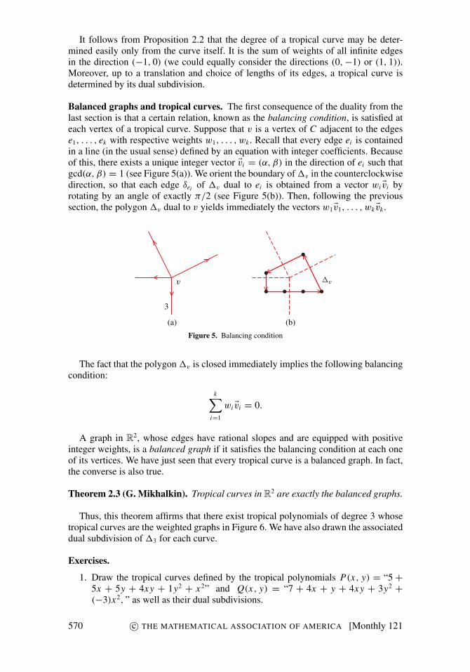
Balanced graphs and tropical curves. The first consequence of the duality from thelast section is that a certain relation, known as the balancing condition, is satisfied ateach vertex of a tropical curve. Suppose that v is a vertex of C adjacent to the edgese1, . . . , ek with respective weights w1, . . . , wk . Recall that every edge ei is containedin a line (in the usual sense) defined by an equation with integer coefficients. Becauseof this, there exists a unique integer vector Evi = (α, β) in the direction of ei such thatgcd(α, β) = 1 (see Figure 5(a)). We orient the boundary of1v in the counterclockwisedirection, so that each edge δei of 1v dual to ei is obtained from a vector wi Evi byrotating by an angle of exactly π/2 (see Figure 5(b)). Then, following the previoussection, the polygon 1v dual to v yields immediately the vectors w1Ev1, . . . , wk Evk .

3

v 1v

(a) (b)

Figure 5. Balancing condition

The fact that the polygon1v is closed immediately implies the following balancingcondition:

k∑i=1

wi Evi = 0.

A graph in R2, whose edges have rational slopes and are equipped with positiveinteger weights, is a balanced graph if it satisfies the balancing condition at each oneof its vertices. We have just seen that every tropical curve is a balanced graph. In fact,the converse is also true.

Theorem 2.3 (G. Mikhalkin). Tropical curves in R2 are exactly the balanced graphs.

Thus, this theorem affirms that there exist tropical polynomials of degree 3 whosetropical curves are the weighted graphs in Figure 6. We have also drawn the associateddual subdivision of 13 for each curve.

Exercises.

1. Draw the tropical curves defined by the tropical polynomials P(x, y) = “5 +5x + 5y + 4xy + 1y2 + x2” and Q(x, y) = “7 + 4x + y + 4xy + 3y2 +(−3)x2, ” as well as their dual subdivisions.


2

(a) (b) (c)

Figure 6.

2. A tropical triangle is a domain of R2 bounded by three tropical lines. What arethe possible forms of a tropical triangle?

3. Prove Proposition 2.2.4. Show that a tropical curve of degree d has at most d2 vertices.5. Find an equation for each of the tropical curves in Figure 6. The following re-

minder might be helpful: If v is a vertex of a tropical curve defined by a tropicalpolynomial P(x, y), then the value of P(x, y) in a neighborhood of v is givenuniquely by the monomials corresponding to the polygon dual to v.

3. TROPICAL INTERSECTION THEORY.

Bezout’s theorem. One of the main interests in tropical geometry is to provide asimple model of algebraic geometry. For example, the basic theorems from intersec-tion theory of tropical curves require much less mathematical background than theirclassical counterparts. The theorem we have in mind is Bezout’s theorem, which statesthat two algebraic curves in the plane of degrees d1 and d2, respectively, intersect ind1d2 points.7 Before we tackle the general case, let us first consider tropical lines andconics.

As mentioned in the introduction, two tropical lines generally intersect in exactlyone point (see Figure 7(a)), just as in classical geometry. Now, do a tropical line anda tropical conic intersect each other in two points? If we naively count the numberof intersection points, the answer is sometimes yes (Figure 7(b)) and sometimes no(Figure 7(c)).

(a) (b) (c)

Figure 7. Intersections of tropical lines and conics

7Warning, this is a theorem in projective geometry! For example, we may have two lines in the classicalplane that are parallel: If they do not intersect in the plane, they intersect nevertheless at infinity. Also, we haveto count intersection points with multiplicity. For example, a tangency point between two curves will count astwo intersection points.


In fact, the unique intersection point of the conic and the tropical line in Figure 7(c)should be counted twice. But why twice in this case and not in the previous case? Tofind the answer, we look to the dual subdivisions.

We start by restricting to the case when the curves C1,C2 intersect in a finite col-lection of points away from the vertices of both curves. Note that the union of the twotropical curves C1 and C2 is again a tropical curve. In fact, we can easily verify that theunion of two balanced graphs is again a balanced graph. Or, we could also easily checkthat if C1 and C2 are defined by tropical polynomials P1(x, y), P2(x, y), respectively,then Q(x, y) = “P1(x, y)P2(x, y)” defines precisely the curve C1 ∪ C2. Moreover, thedegree of C1 ∪ C2 is the sum of the degrees of C1 and C2.

The dual subdivisions of the unions of the two curves C1 and C2 in the three casesof Figure 7 are represented in Figure 8. In every case, the set of vertices of C1 ∪ C2 isthe union of the vertices of C1, the vertices of C2, and the intersection points of C1 andC2. Moreover, since each point of intersection of C1 and C2 is contained in an edge ofboth C1 and C2, the polygon dual to such a vertex of C1 ∪ C2 is a parallelogram. Tomake Figure 8 more transparent, we have drawn each edge of the dual subdivision inthe same color as its corresponding dual edge. We can conclude that in Figures 8(a)and (b), the corresponding parallelograms are of area one, whereas the correspondingparallelogram of the dual subdivision in Figure 8(c) has area two! Hence, it seems thatwe are counting each intersection point with the multiplicity we will describe below.

(a) (b) (c)

Figure 8. The subdivisions dual to the union of the curves in Figure 7

Definition 3.1. Let C1 and C2 be two tropical curves that intersect in a finite numberof points and away from the vertices of the two curves. If p is a point of intersectionof C1 and C2, the tropical multiplicity of p as an intersection point of C1 and C2 is thearea of the parallelogram dual to p in the dual subdivision of C1 ∪ C2.

With this definition, proving the tropical Bezout’s theorem is a walk in the park!

Theorem 3.2 (B. Sturmfels). Let C1 and C2 be two tropical curves of degrees d1 andd2 respectively, intersecting in a finite number of points away from the vertices of thetwo curves. Then the sum of the tropical multiplicities of all points in the intersectionof C1 and C2 is equal to d1d2.

Proof. Let us call this sum of multiplicities s. Notice that there are three types ofpolygons in the subdivision dual to the tropical curve C1 ∪ C2:

• those dual to a vertex of C1. The sum of their areas is equal to the area of 1d1 , in

other words,d2

12 ;

• those dual to a vertex of C2. The sum of their areas is equal tod2

22 ;


• those dual to an intersection point of C1 and C2. The sum of their areas we havecalled s.

Since the curve C1 ∪ C2 is of degree d1 + d2, the sum of the area of all of these poly-

gons is equal to the area of 1d1+d2 , which is (d1+d2)2

2 . Therefore, we obtain

s = (d1 + d2)2 − d2

1 − d22

2= d1d2,

which completes the proof.

Stable intersection. In the last section, we considered only tropical curves that inter-sect “nicely”, meaning they intersect only in a finite number of points and away fromthe vertices of the two curves. But what can we say in the two cases shown in Fig-ures 9(a) (two tropical lines that intersect in an edge) and 9(b) (a tropical line passingthrough a vertex of a conic)? Thankfully, we have more than one tropical trick up oursleeve.

εv

εv

(a) (b) (c) (d)

Figure 9. Non-transverse intersection and a translation

Let ε be a very small positive real number and Ev a vector such that the quotient ofits two coordinates is an irrational number. If we translate in each of the two casesone of the two curves in Figures 9(a) and (b) by the vector εEv, we find ourselves backin the case of “nice” intersection (see Figures 9(c) and (d)). Of course, the resultingintersection depends on the vector εEv. On the other hand, the limit of these points, ifwe let ε shrink to 0, does not depend on Ev. The points in the limit are called the stableintersection points of two curves. The multiplicity of a point p in the stable intersectionis equal to the sum of the intersection multiplicities of all points that converge to pwhen ε tends to zero.

For example, there is only one stable intersection point of the two lines in Figure9(a). The point is the vertex of the line on the left. Moreover, this point has multiplic-ity 1, so again, our two tropical lines intersect in a single point. The point of stableintersection of the two curves in Figure 9(b) is the vertex of the conic, and it has mul-tiplicity 2.

Notice that if a point is in the stable intersection of two tropical curves, then it iseither an isolated intersection point, or a vertex of one of the two curves. Thanks tostable intersection, we can remove from our previous statement of the tropical Bezouttheorem the hypothesis that the curves must intersect “nicely”.

Theorem 3.3 (B. Sturmfels). Let C1 and C2 be two tropical curves of degree d1 andd2. Then the sum of the multiplicities of the stable intersection points of C1 and C2 isequal to d1d2.


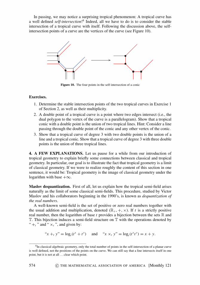
In passing, we may notice a surprising tropical phenomenon: A tropical curve hasa well defined self-intersection!8 Indeed, all we have to do is to consider the stableintersection of a tropical curve with itself. Following the discussion above, the self-intersection points of a curve are the vertices of the curve (see Figure 10).

Figure 10. The four points in the self-intersection of a conic

Exercises.

1. Determine the stable intersection points of the two tropical curves in Exercise 1of Section 2, as well as their multiplicity.

2. A double point of a tropical curve is a point where two edges intersect (i.e., thedual polygon to the vertex of the curve is a parallelogram). Show that a tropicalconic with a double point is the union of two tropical lines. Hint: Consider a linepassing through the double point of the conic and any other vertex of the conic.

3. Show that a tropical curve of degree 3 with two double points is the union of aline and a tropical conic. Show that a tropical curve of degree 3 with three doublepoints is the union of three tropical lines.

4. A FEW EXPLANATIONS. Let us pause for a while from our introduction oftropical geometry to explain briefly some connections between classical and tropicalgeometry. In particular, our goal is to illustrate the fact that tropical geometry is a limitof classical geometry. If we were to realize roughly the content of this section in onesentence, it would be: Tropical geometry is the image of classical geometry under thelogarithm with base +∞.

Maslov dequantization. First of all, let us explain how the tropical semi-field arisesnaturally as the limit of some classical semi-fields. This procedure, studied by VictorMaslov and his collaborators beginning in the 1990’s, is known as dequantization ofthe real numbers.

A well-known semi-field is the set of positive or zero real numbers together withthe usual addition and multiplication, denoted (R+,+,×). If t is a strictly positivereal number, then the logarithm of base t provides a bijection between the sets R andT. This bijection induces a semi-field structure on T with the operations denoted by“+t ” and “×t ”, and given by:

“x +t y” = logt(tx + t y) and “x ×t y” = logt(t

x t y) = x + y.

8In classical algebraic geometry, only the total number of points in the self-intersection of a planar curveis well defined, not the positions of the points on the curve. We can still say that a line intersects itself in onepoint, but it is not at all . . . clear which point.


The equation on the right-hand side already shows classical addition appearing asan exotic kind of multiplication on T. Notice that by construction, all of the semi-fields(T, “ +t ”, “ ×t ”) are isomorphic to (R+,+,×). The trivial inequality max(x, y) ≤x + y ≤ 2 max(x, y) on R+, together with the fact that the logarithm is an increasingfunction, gives us the following bounds for “+t ”:

∀t > 1, max(x, y) ≤ “x +t y” ≤ max(x, y)+ logt 2.

If we let t tend to infinity, then logt 2 tends to 0, and the operation “ +t ” thereforetends to the tropical addition “+ ”! Hence, the tropical semi-field comes naturally fromdegenerating the classical semi-field (R+,+,×). From an alternative perspective, wecan view the classical semi-field (R+,+,×) as a deformation of the tropical semi-field. This explains the use of the term “dequantization”, coming from physics andreferring to the procedure of passing from quantum to classical mechanics.

Dequantization of a line in the plane. Now we will apply a similar reasoning to theline in the plane R2 defined by the equation x − y + 1 (see Figure 11(a)). To apply thelogarithm map to the coordinates of R2, we must first take their absolute values. Doingthis results in folding the four quadrants of R2 onto the positive quadrant (see Figure11(b)). The image of the folded-up line under the coordinate-wise logarithm with baset applied to (R∗+)2 is drawn in Figure 11(c). By definition, taking the logarithm withbase t is the same thing as taking the natural logarithm and then rescaling the result bya factor of 1

ln t . Thus, as t increases, the image under the logarithm with base t of theabsolute value of our line becomes concentrated around a neighborhood of the originand three asymptotic directions, as shown in Figures 11(c), (d), and (e). If we allow tto go all the way to infinity, then we see the appearance in Figure 11(f) of a tropicalline!

(a) (b) (c)

(d) (e) (f)

Figure 11. Dequantization of a line

5. PATCHWORKING. Reading Figure 11 from left to right, we see how startingfrom a classical line in the plane we can arrive at a tropical line. Reading this figurefrom right to left is, in fact, much more interesting. Indeed, we see as well how toconstruct a classical line given a tropical one. The technique known as patchworking


is a generalization of this observation. In particular, it provides a purely combinatorialprocedure to construct real algebraic curves from a tropical curve. To explain thisprocedure in more detail, we first go a bit back in time.

Hilbert’s 16th problem. A planar real algebraic curve is a curve in the plane R2

defined by an equation of the form P(x, y) = 0, where P(x, y) is a polynomial whosecoefficients are real numbers. The real algebraic curves of degree 1 and 2 are simpleand well known; they are lines and conics, respectively. When the degree of P(x, y)increases, the form of the real algebraic curve can become more and more complicated.If you are not convinced, take a look at Figure 12, which shows some of the possibledrawings realized by real algebraic curves of degree 4.

(a) (b) (c) (d)

Figure 12. Some real algebraic curves of degree 4

A theorem due to Axel Harnack at the end of the 19th century states that a planarreal algebraic curve of degree d has a maximum of d(d−1)+2

2 connected components.But how can these components be arranged with respect to each other? We call therelative position of the connected components of a planar real algebraic curve in theplane its arrangement. In other words, we are not interested in the exact position ofthe curve in the plane, but simply in the configuration that it realizes. For example, ifone curve has two bounded connected components, we are only interested in whetherone of these components is contained in the other (Figure 12(c)) or not (Figure 12(a)).At the second International Congress in Mathematics in Paris in 1900, David Hilbertannounced his famous list of 23 problems for the 20th century. The first part of his16th problem can be very widely understood as the following:

Given a positive integer d, establish a list of possible arrangements of real alge-braic curves of degree d.

At Hilbert’s time, the answer9 was known for curves of degree at most 4. Therehave been spectacular advances in this problem in the 20th century, due mostly in partto mathematicians from the Russian school. Despite this, there remain numerous openquestions.

Real and tropical curves. In general, it is a difficult problem to construct a real alge-braic curve of a fixed degree and realizing a given arrangement. For a century, math-ematicians have proposed many ingenious methods for doing this. The patchworkingmethod invented by Oleg Viro in the quantization is actually one of the most powerful.

9A more reasonable and natural problem is to consider arrangements of connected components of non-singular real algebraic curves in the projective plane, rather than in R2. In this more restrictive case, the answerwas known up to degree 5 in Hilbert’s time, and is now known up to degree 7. The list in degree 7 is given ina theorem by Oleg Viro and patchworking is an essential tool in its proof.


At this time, tropical geometry was not yet in existence, and Viro announced his the-orem in a language different from what we use here. However, he realized by the endof the 1990’s that his patchworking could be interpreted as a quantization of tropicalcurves. Patchworking is, in fact, the process of reading Figure 11 from right to leftinstead of left to right. Thanks to the interpretation of patchworking in terms of tropi-cal curves, shortly afterwards, Grigory Mikhalkin generalized Viro’s original method.Here we will present a simplified version of patchworking. The interested reader mayfind a more complete version in the references indicated in Section 7.

In what follows, for a, b two integer numbers, we denote by sa,b : R2 → R2 thecomposition of a reflections in the x-axis with b reflections in the y-axis. Therefore,the map sa,b depends only on the parity of a and b. To be precise, s0,0 is the identity,s1,0 the reflection in the x-axis, s0,1 the reflection in the y-axis, and s1,1 the reflectionin the origin (equivalently, rotation by 180 degrees).

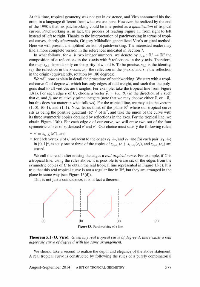
We will now explain in detail the procedure of patchworking. We start with a tropi-cal curve C of degree d , which has only edges of odd weight, and such that the poly-gons dual to all vertices are triangles. For example, take the tropical line from Figure13(a). For each edge e of C , choose a vector Eve = (αe, βe) in the direction of e suchthat αe and βe are relatively prime integers (note that we may choose either Eve or −Eve,but this does not matter in what follows). For the tropical line, we may take the vectors(1, 0), (0, 1), and (1, 1). Now, let us think of the plane R2 where our tropical curvesits as being the positive quadrant (R∗+)2 of R2, and take the union of the curve withits three symmetric copies obtained by reflections in the axes. For the tropical line, weobtain Figure 13(b). For each edge e of our curve, we will erase two out of the foursymmetric copies of e, denoted e′ and e′′. Our choice must satisfy the following rules:

• e′ = sαe,βe(e′′), and

• for each vertex v of C adjacent to the edges e1, e2, and e3, and for each pair (ε1, ε2)

in {0, 1}2, exactly one or three of the copies of sε1,ε2(e1), sε1,ε2(e2), and sε1,ε2(e3) areerased.

We call the result after erasing the edges a real tropical curve. For example, if C isa tropical line, using the rules above, it is possible to erase six of the edges from thesymmetric copies of C to obtain the real tropical line represented in Figure 13(c). It istrue that this real tropical curve is not a regular line in R2, but they are arranged in theplane in same way (see Figure 13(d)).

This is not just a coincidence; it is in fact a theorem.

(a) (b) (c) (d)

Figure 13. Patchworking of a line

Theorem 5.1 (O. Viro). Given any real tropical curve of degree d, there exists a realalgebraic curve of degree d with the same arrangement.

We should take a second to realize the depth and elegance of the above statement.A real tropical curve is constructed by following the rules of a purely combinatorial


game. It seems like magic to assert that there is a relationship between these combi-natorial objects and actual real algebraic curves! We will not get into details here, butViro’s method even allows us to determine the equation of a real algebraic curve withthe same arrangement than a given real tropical curve.

Of course, much skill and intuition are still required to construct real algebraiccurves with complicated arrangements, and both of these are acquired with practice.Therefore, we invite the reader to try the exercises at the end of this section. Neverthe-less, patchworking provides a much more flexible technique to construct arrangementsthan dealing directly with polynomials. In particular, it requires no a priori knowledgeof algebraic geometry. To illustrate the use of Viro’s patchworking, let us now con-struct the arrangements of two real algebraic curves, one of degree 3 and the other ofdegree 6.

First of all, consider the tropical curve of degree 3 shown in Figure 14(a). For suit-able choices of edges to erase, Figures 14(b) and (c) represent the two stages of thepatchworking procedure. With this, we have proved the existence of a real algebraiccurve of degree 3, resembling the configuration of Figure 14(d).

(a) (b) (c) (d)

Figure 14. Patchworking of a cubic

To conclude, consider the tropical curve of degree 6 drawn in Figure 15(a). Onceagain, for a suitable choice of edges to erase, the patchworking procedure gives thecurve in Figure 15(c). A real algebraic curve of degree 6 that realizes the same arrange-ment as the real tropical curve was first constructed by using much more complicatedtechniques in the 1960’s by Gudkov. An interesting piece of trivia: Hilbert announcedin 1900 that such a curve could not exist!

(a) (b) (c)

Figure 15. Gudkov’s curve


Amoebas. Even though dequantization of a line is the main idea underlying patch-working in its full generality, the proof of Viro’s theorem is quite a bit more technicalto explain rigorously. Here, we will give a sketch of what is involved in the proof.

First of all, since the field R is not algebraically closed, we will not work with realalgebraic curves but rather complex algebraic curves, in other words, subsets of thespace (C∗)2 defined by equations of the form P(x, y) = 0, where C∗ = C \ {0}, andP(x, y) is a polynomial with complex coefficients (which can therefore be real). For ta positive real number, we define the map Logt on (C∗)2 by

Logt (C∗)2 −→ R2

(x, y) 7−→ (logt |x |, logt |y|).

We denote the image of a curve given by the equation P(x, y) = 0 under the mapLogt by At(P), and call it the amoeba of base t of the curve. Exactly as in Section 4,the limit of At(P) when t goes to +∞ is a tropical curve having a single vertex, withinfinite rays corresponding to asymptotic directions of the amoebas At(P). However,we can obtain more interesting limiting objects by considering families of algebraiccurves, that is to say, for each t , not only the base of the logarithm changes, but also thecurve whose amoeba we are considering. Such a family of complex algebraic curvestakes the form of a polynomial Pt(x, y), whose coefficients are given as functions ofthe real number t . Therefore, for each choice of t > 1 we obtain an honest polynomialin x and y that defines a curve in the plane.

The following theorem says that all tropical curves arise as the limit of amoebasof families of complex algebraic curves, and provides a fundamental link betweenclassical algebraic geometry and tropical geometry.

Theorem 5.2 (G. Mikhalkin, H. Rullgard). Let P∞(x, y) = “∑

i, j ai, j x i y j ” be atropical polynomial. For each coefficient ai, j different from −∞, choose a finite setIi, j ⊂ R such that ai, j = max Ii, j , and choose αi, j (t) =

∑r∈Ii, j

βi, j,r tr with βi, j,r 6= 0.

For every t > 0, we define the complex polynomial Pt(x, y) =∑i, j αi, j (t)x i y j . Thenthe amoeba At(Pt) converges to the tropical curve defined by P∞(x, y) when t tendsto +∞.

The dequantization of the curve seen in Section 4 is a particular case of the abovetheorem. The amoeba of base t of the line with equation t0x − t0 y + t01 = 0 con-verges to the tropical line defined by “0x + 0y + 0”. We can deduce Viro’s theoremfrom the preceding theorem by remarking, among other details, that if the βi, j,r arereal numbers, then the curves defined by the polynomials Pt(x, y) are real algebraiccurves.

Exercises.

1. Construct a real tropical curve of degree 2 that realizes the same arrangement asa hyperbola in R2. Do the same for a parabola. Can we construct a real tropicalcurve realizing the same arrangement as an ellipse?

2. By using patchworking, show that there exists a real algebraic curve of degree 4realizing the arrangement shown in Figure 12(b). Use the construction illustratedin Figure 14 as a guide.

3. Show that for every degree d , there is a real algebraic curve with d(d−1)+22 con-

nected components.


6. FURTHER DIRECTIONS. So far, we only considered tropical polynomials inone variable, their tropical roots, and tropical curves in the plane. Tropical geometry,however, extends far beyond these basic objects, and we would like to showcase brieflysome horizons that fit within the topics of the material discussed in this text.

Hyperfields. Recall that we started our tour of tropical geometry by introducing thetropical semi-field T, which we obtained from the real numbers by Maslov’s dequanti-zation procedure. We then proceeded to consider the solutions to polynomial equationsover this semi-field by choosing our definitions wisely. Since the appearance of tropi-cal algebra, there have been several proposals to enrich this simple tropical semi-fieldto other algebraic structures, in order to better understand relations between tropicalalgebra and geometry. Here, we present an example of such an enrichment, suggestedby Viro, known as hyperfields.

Similarly to a field, a hyperfield is a set equipped with two operations called mul-tiplication and addition, which satisfy some axioms. The main difference between hy-perfields and (semi-)fields is that addition is allowed to be multivalued; this meansthat the sum of two numbers is not necessarily just one number as we are used to,but can actually be a set of numbers. The simplest hyperfield is the sign hyperfield,which consists of only three elements 0, +1, and −1. The multiplication is as usual,i.e., (−1)× (−1) = 1, but the multivalued addition is defined by the following table.In fact, this hyperfield is quite natural. Suppose you were to add or multiply two realnumbers but you only knew their signs; then the corresponding operations of the signedhyperfield give all the possible signs of the output.

+ 0 +1 −1

0 {0} {+1} {−1}+1 {+1} {+1} {0,±1}−1 {−1} {0,±1} {−1}

There exist several hyperfields related to tropical geometry. Here we will show justone, which resembles our tropical semi-field quite a bit. It consists of the same under-lying set T = R ∪ {−∞}, and multiplication is again the usual addition. However, themultivalued addition is now the following:

x y ={{max(x, y)}, if x 6= y,{z ∈ T | z ≤ x}, if x = y.

Notice that −∞ can still be considered as the tropical zero, since x −∞ = {x} forany x ∈ T.

Let us take a look at how this foreign concept of multivalued addition can simplifysome definitions and resolve some peculiarities in tropical geometry. In the tropicalhyperfield T, we declare x0 to be a root of a tropical polynomial P(x) if the set P(x0)

contains the tropical zero−∞. Notice that both definitions of the roots of a polynomialcoincide, whether it is considered over the tropical hyperfield or the tropical semi-field.

In the case of curves, every classical line in the plane is given by the equationy = ax + b. Points in T2 satisfying the same equation y = “ax + b” = max(a + x, b)over the tropical semi-field form a piecewise linear graph, as depicted in Figure 2(a).However, this is not at all a tropical curve, as the balancing condition is not satisfied


at (b − a, b), where the linearity breaks. If, instead, we replace our semi-field addi-tion with the new mutlivalued hyperfield addition, then there is one point where thefunction P(x) = (a + x) b is truly multivalued:

P(b − a) = {x ∈ R ∪ {−∞} | x ≤ b} .

Hence, the previous graph grows a vertical tail at x = b − a when the function isconsidered over the tropical hyperfield; this is the dotted line in Figure 2(a). Therefore,we obtain the tropical line that we first encountered in Figure 1.

In conclusion, we see that using the tropical hyperfield already simplifies somebasic aspects of tropical geometry. The definition of the zeroes of polynomials seemsmore natural, and sets in R2 defined by a simple equation of the form y = P(x) aretropical curves, which was not the case over the tropical semi-field.

Tropical modifications. If we compare the above example again to the classical situ-ation, then we may notice another phenomenon particular to tropical geometry. Clas-sically, the shape of a line does not change depending on where it lives. For example, anon-vertical line in R2 projects bijectively to the x-axis; more generally, any line in Rn

is in bijection with a coordinate axis via a projection. This dramatically fails in tropicalgeometry. The projection to the x-axis of a generic tropical line in T2 no longer givesa bijection to T, since the vertical edge of the line is contracted to a point. In general,the possible shapes of a tropical line depend on the space Tn where it sits. We can,nevertheless, describe them all. A generic line in Tn has the shape of a line in Tn−1

with an additional tail grown at an interior point. We depicted in Figure 16 some pos-sible shapes of tropical lines in T3 and T5. Notice that, according to this description, ageneric tropical line in Tn has n + 1 ends, and is always a tree, meaning a graph withno cycles.10

(a) A tropical line in T3 (b) A “snowflake” line in T5 (c) A “caterpillar” line in T5

Figure 16. Different tropical lines

This phenomenon is not specific to tropical lines; in general, there are infinitelymany possible ways of modelling an object from classical geometry by a tropical ob-ject. This presents tropical geometers with some interesting problems, such as the fol-lowing. What do the different tropical models of the same classical object have incommon? How are two different models of the same object related? Does there exist amodel better than the others?

It turns out that different tropical models are related by an operation known as trop-ical modification. In fact, the example we just saw with a tropical line in T2 along withthe projection to T in the vertical direction is precisely a tropical modification of T. Letus take a look at another example in two dimensions. Consider the tropical polynomial

10Alternatively, a tree is a graph in which there is exactly one path joining any two vertices.


in two variables P(x, y) = x y 0 over the tropical hyperfield. The subset 5 of T3

defined11 by z ∈ P(x, y) is drawn in Figure 17. It is a piecewise linear surface with2-dimensional faces; three of them are in the downward vertical direction and arisedue to P(x, y) being multivalued. These six faces are glued along any pair of the fourrays starting at (0, 0, 0) and in the directions

u1 = (−1, 0, 0), u2 = (0,−1, 0), u3 = (0, 0,−1), and u0 = (1, 1, 1).

0

y

x

5

T2

(0,−t, 0)

(t, t, t)

(−t, 0, 0)

(0, 0,−t)

Figure 17. A modification 5 of the tropical affine plane T2

Just as in Section 5, we may consider the limit of amoebas Logt(P) of the planeP ⊂ R3 defined by the equation x + y + z + 1 = 0. This limit is again the piecewiselinear surface5, and therefore this latter provides another tropical model of a classicalplane!12 Notice that once again the projection that forgets the third coordinate, estab-lishes a bijection between P and R2, but is not a bijection between 5 and T2. Thisprojection map 5 −→ T2 is a tropical modification of the tropical plane T2.

We might ask why we would want to use this more complicated model5 of a planerather than just T2. Let us show an example. Consider the real line

L = {(x, y) ∈ R2 | x + y + 1 = 0} ⊂ R2,

11Here, we use the tropical hyperfield for consistency. Alternatively, definitions of Sections 1 and 2 admitnatural generalizations to polynomials with any number of variables, and 5 is the tropical surface defined bythe tropical polynomial “0+ x + y + z”.

12The same phenomenon as in the case of curves happens here. We may consider for simplicity a plane inR3, because it is defined by a linear equation. However, if we want to study tropical surfaces of higher degreeand their approximations by amoebas of classical surfaces as in Theorem 5.2, then we have to leave R for itsalgebraic closure C.


and let L ⊂ T2 be the corresponding tropical line, i.e., L = limt→+∞ Logt(L). Let L′tbe a family of lines in R2 whose amoebas converge to some tropical line L ′ ⊂ T2 asin Theorem 5.2, and define pt = L ∩ L′t . Now, let us ask the following question: Canwe determine limt→+∞ Logt(pt) by only looking at the tropical picture?

If the set-theoretic intersection of L and L ′ consists of a single point p, thenLogt(pt) has no choice but to converge to p. But what happens when this set-theoreticintersection is infinite?

Suppose that L ′ is given by the tropical polynomial “1 · x + y + 0”, so that theposition of L and L ′ is as in Figure 9(a) with L in blue and L ′ in red. Then the stableintersection of L and L ′ is the vertex of L ′, that is to say the point (−1, 0). Note thatthis is independent of the family L′t , as long as Logt(L′t) converges to L ′. However,depending on the family L′t , the point limt→+∞ Logt(pt) may be located anywhere onthe half-line {(x, 0),−∞ ≤ x ≤ −1}. Indeed, given the family

L′t ={(x, y) ∈ R2 | (t + 1)x + y + (1− tb+1) = 0

}with b ≤ −1,

then by Theorem 5.2, limt→+∞ Logt(L′t) = L ′. Yet we have pt = (tb,−1− tb), and solimt→+∞ Logt(pt) = (b, 0). Similarly, we get limt→+∞ Logt(pt) = (−∞, 0) by taking

L′t ={(x, y) ∈ R2 | t x + y + 1 = 0

}.

This shows that using the tropical model L , L ′ ∈ T2, it is impossible to extract in-formation about the location of the intersection point of L and L′t . It turns out thatchanging the model T2 via a tropical modification unveils the location of the limit ofthe intersection point pt . To obtain our new model, let us consider again the planeP ⊂ R3 with equation x + y + z + 1 = 0, and the projection

π : P −→ R2

(x, y, z) 7−→ (x, y).

The map π is clearly a bijection, and π−1(x, y) = (x, y,−x − y − 1). The inter-section of P with the plane z = 0 in R3 is precisely the line L. This implies thatLogt(π

−1(L)) ⊂ {z = −∞} and

limt→+∞

Logt(π−1(L)) = 5 ∩ {z = −∞} ⊂ T3.

If L′t is a family of lines in R2 as above, then π−1(L′t) is a family of lines in P , and,moreover, the intersection point pt must satisfy π−1(pt) ∈ {z = 0}. In particular, wehave

limt→+∞

Logt(π−1(pt)) ∈ {z = −∞}.

Now it turns out that L ′′ = limt→+∞ Logt(π−1(L′t)) is a tropical line in 5, which

intersects the plane {z = −∞} in a single point! Therefore, upon projection back toR2, this point is nothing else but limt→+∞ Logt(pt); in other words, the location oflimt→+∞ Logt(pt) is now revealed by considering the tropical picture in T3. In Figure18 we depict the case when L′t is given by (t + 1)x + y + (1− tb+1) = 0.

Hence, there is no unique or canonical choice of a tropical model of a classicalspace, and tropical modification is the tool used to pass between the different models.There is a single space that captures in a sense all the possible tropical models, known


L

L′′

(b, 0, –∞)

Figure 18. The tropical lines L and L ′′ in the modified plane 5

as the Berkovich space of the classical object. The structure of a Berkovich space isextremely complicated due to the infinitely many different tropical models. For ex-ample, the Berkovich line is an infinite tree. In a sense, a tropical model gives us justa snapshot of the complicated Berkovich space and modifications are what allow us tochange the resolution.

Higher (co)dimension. In the first part of this text, our main object of study wastropical curves in the plane. Even in this limited case, there are many applicationsto classical geometry. In higher dimensions, things become a bit trickier as the linksbetween the tropical and classical worlds become more intricate.

As we mentioned earlier, the definitions of Sections 1 and 2, as well as Theorem 5.2,admit natural generalizations to polynomials with any number of variables. A tropicalpolynomial in n variables P(x1, . . . , xn) defines a tropical hypersurface in Tn , whichis the corner locus of the graph of P equipped with some weights. A tropical hypersur-face in Tn is glued from flat pieces, has dimension n − 1, satisfies a balancing conditionsimilar to curves, and arises as the limit of amoebas of a family of complex hypersur-faces. Because of this, we say that all tropical hypersurfaces are approximable.

It is also natural to consider tropical objects of dimension less than n − 1 in Tn . Ak-dimensional tropical variety is a weighted polyhedral complex of dimension k, sat-isfying a generalization of the balancing condition that we saw for curves. It would betoo technical and probably useless to give here the balancing condition in full general-ity. Nevertheless, in the case of curves, i.e., when k = 1, the definition is the same as inSection 2: A tropical curve in Rn is a graph whose edges have a rational direction andare equipped with positive integer weights. In addition, the graph must satisfy the bal-ancing condition given in Section 2 at each vertex. Unfortunately, Theorem 5.2 doesnot generalize to the case of higher codimensions. There exist tropical varieties, said tobe not approximable, which do not arise as limits of amoebas of complex varieties ofthe same degree. For our purposes, we may think of a complex variety in Cn as beingthe solution set of a system of polynomial equations in n variables.

Already in T3 there are many examples of tropical curves that are not approximable.More intricately, there are examples of pairs of tropical varieties Y ⊂ X ⊂ Tn forwhich both Y and X are approximable independently; however, there do not exist


approximations Yt and Xt of Y and X with Yt ⊂ Xt . Let us give an explicit exampleof such a pair.

Consider the modified tropical plane 5 ⊂ T3 we just encountered, which is ap-proximated by the amoebas of the complex plane P ⊂ C3 defined by the equationx + y + z + 1 = 0. Now, the union of three rays in the directions

(−2,−3, 0), (0, 1, 1), (2, 2,−1)

with each ray equipped with weight 1 is a tropical curve C ⊂ T3. We may check thatthe balancing condition is satisfied:

(−2,−3, 0)+ (0, 1, 1)+ (2, 2,−1) = 0.

Moreover, C is contained in the tropical plane 5, since we may express the three raysas

(−2,−3, 0) = 2u1 + 3u2, (0, 1, 1) = u0 + u1, (2, 2,−1) = 2u0 + 3u3,

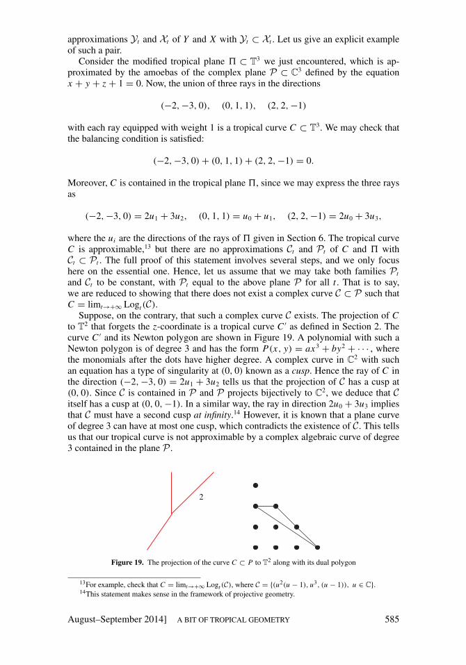
where the ui are the directions of the rays of 5 given in Section 6. The tropical curveC is approximable,13 but there are no approximations Ct and Pt of C and 5 withCt ⊂ Pt . The full proof of this statement involves several steps, and we only focushere on the essential one. Hence, let us assume that we may take both families Pt

and Ct to be constant, with Pt equal to the above plane P for all t . That is to say,we are reduced to showing that there does not exist a complex curve C ⊂ P such thatC = limt→+∞ Logt(C).

Suppose, on the contrary, that such a complex curve C exists. The projection of Cto T2 that forgets the z-coordinate is a tropical curve C ′ as defined in Section 2. Thecurve C ′ and its Newton polygon are shown in Figure 19. A polynomial with such aNewton polygon is of degree 3 and has the form P(x, y) = ax3 + by2 + · · · , wherethe monomials after the dots have higher degree. A complex curve in C2 with suchan equation has a type of singularity at (0, 0) known as a cusp. Hence the ray of C inthe direction (−2,−3, 0) = 2u1 + 3u2 tells us that the projection of C has a cusp at(0, 0). Since C is contained in P and P projects bijectively to C2, we deduce that Citself has a cusp at (0, 0,−1). In a similar way, the ray in direction 2u0 + 3u3 impliesthat C must have a second cusp at infinity.14 However, it is known that a plane curveof degree 3 can have at most one cusp, which contradicts the existence of C. This tellsus that our tropical curve is not approximable by a complex algebraic curve of degree3 contained in the plane P .

2

Figure 19. The projection of the curve C ⊂ P to T2 along with its dual polygon

13For example, check that C = limt→+∞ Logt (C), where C = {(u2(u − 1), u3, (u − 1)), u ∈ C}.14This statement makes sense in the framework of projective geometry.


Many other examples of non-approximable tropical objects exist, including lines insurfaces, curves in space, and even linear spaces. What must be stressed is that, froma purely combinatorial viewpoint, it is very difficult to distinguish these pathologicaltropical objects from approximable ones. This is just one of the problems that makestropical geometry continue to be a challenging and exciting field of research, especiallyin terms of its relations to classical geometry.

7. REFERENCES. The references given below contain the proofs of statements con-tained throughout the text. They also present the many directions in which tropical ge-ometry is developing. The references to the literature go far beyond what we mentionhere; it would be impossible to provide a complete list. However, we hope to give anaccount of the multitude of perspectives on tropical geometry.

First, we should note that tropical curves first appeared under the name of (p, q)-webs, in the work of the physicists O. Aharony, A. Hanany, and B. Kol [2]. In mathe-matics, roots of tropical geometry can be traced back at least to the work of Bergman[8] on logarithmic limit sets of algebraic varieties, to Bieri and Groves [10] on non-archimedean valuations, to Viro on patchworking (see references below), as well to thestudy of toric varieties, which provide a first relation between convex polytopes andalgebraic geometry, see for example [17], [19].

There are other general introductions to tropical geometry. The texts [9] and [49]are aimed at the interested reader with a minimal background in mathematics, similarto the one assumed in this text. There the authors emphasize different applicationsof tropical geometry, enumerative geometry in [9], and phylogenetics in [49]. Moreconfident readers can also read the works of [20], [24], [25], [30], [31], [36], [37], and[46]. For established geometers, we recommend the state of the art [33] and [35].

In particular, stable intersections of tropical curves in R2 are discussed in detailin [46]. The proof of the Bezout theorem we gave is contained in [20]. Foundationsof a more sophisticated tropical intersection theory are exposed in [35], and furtherdeveloped in [4], [28], [47].

Amoebas of algebraic varieties were introduced in [22]. The interested reader canalso see the texts [43], [56], and the more sophisticated [42]. For a deeper look atpatchworking, amoebas, and Maslov’s dequantization, as well as their applications toHilbert’s 16th problem, we point you to the texts [32], [33], [55], and [57], as well asthe website [59]. We especially recommend the text [26], dedicated to a large audience,which explains how patchworking has been used to disprove the Ragsdale conjecture,which had been open for decades.

For more on tropical hyperfields, we point the reader toward [58]. As we men-tioned in the text, there are other enrichments of the tropical semi-field, some examplesof which can be found in [14], [18], and [27]. Tropical modifications were intro-duced by Mikhalkin in the above-mentioned text [35], and their relations to Berkovichspaces can be found in [44] and [45]. This perspective from Berkovich spaces al-lows one to relate tropical geometry to algebraic geometry, not only over C, butalso over any field equipped with a so-called non-archimedean valuation (e.g., thep-adic numbers equipped with the p-adic valuation). For this point of view, we re-fer, for example, to [1], [7], [40], and references therein. The approximation prob-lem has been studied mostly in the case of curves. For tropical curves, see [5], [29],[34], [35], [38], [39], [48], and [52]. For a look at the approximation problem ofcurves in surfaces, as in the example provided in the last section, see [11], [13], and[21]. Among all sources of motivation to study the latter problem, we recommendthe very nice study of tropical lines in tropical surfaces in R3 by Vigeland in [53]and [54].


To end this introduction to tropical geometry, we point out that this subject hasvery successful applications in many fields other than Hilbert’s 16th problem, suchas enumerative geometry [34], algebraic geometry [51], mirror symmetry [23], mathe-matical biology [6], [41], computational complexity [3], computational geometry [16],[50], and algebraic statistics [15], [41], just to name a few.

ACKNOWLEDGMENT. We are very grateful to Oleg Viro for his encouragement and extremely helpfulcomments. We also thank Ralph Morisson and the anonymous referees for their useful suggestions on a pre-liminary version of this text.

REFERENCES

1. D. Abramovich, L. Caporaso, S. Payne, The tropicalization of the moduli space of curves (2012), avail-able at http://arxiv.org/abs/1212.0373.

2. O. Aharony, A. Hanany, B. Kol, Webs of (p,q) 5-branes, five dimensional field theories and grid diagrams,J. High Energy Phys. 1 (1998) 1–50.

3. M. Akian, S. Gaubert, A. Guterman, Tropical polyhedra are equivalent to mean payoff games, Internat.J. Algebra Comput. 22 (2012) 1250001, available at http://arxiv.org/abs/0912.2462.

4. L. Allermann, J. Rau, First steps in tropical intersection theory, Math. Z. 264 (2010) 633–670.5. O. Amini, M. Baker, E. Brugalle, J. Rabinoff, Lifting harmonic morphisms of tropical curves, metrized

complexes, and Berkovich skeleta (2013), available at http://arxiv.org/abs/1303.4812.6. F. Ardila, C.J. Klivans, The Bergman complex of a matroid and phylogenetic trees, J. Comb. Theory Ser.

B 96 (2006) 38–49.7. M. Baker, S. Payne, J. Rabinoff, Nonarchimedean geometry, tropicalization, and metrics on curves

(2011), available at http://arxiv.org/abs/1104.0320.8. G. M. Bergman, The logarithmic limit-set of an algebraic variety, Trans. Amer. Math. Soc. 157 (1971)

459–469.9. Geometrie Tropicale. Edited by N. Berline, A. Plagne, and C. Sabbah. Editions de l’Ecole Polytechnique,

Palaiseau, 2008.10. R. Bier, J. Groves, The geometry of the set of characters induced by valuations, J. Reine Angew. Math.

347 (1984) 168–195.11. T. Bogart, E. Katz, Obstructions to lifting tropical curves in surfaces in 3-space, SIAM J. Discrete Math.

26 (2012) 1050–1067.12. E. Brugalle, Un peu de geometrie tropicale, Quadrature 74 (2009) 10–22.13. E. Brugalle, K. Shaw, Obstructions to approximating tropical curves in surfaces via intersection theory

(2011), available at http://arxiv.org/abs/arXiv:1110.0533.14. A. Connes, C. Consani, The universal thickening of the field of real numbers (2012), http://arxiv.

org/abs/arXiv:1202.4377.15. M. A. Cueto, J. Morton, B. Sturmfels, Geometry of the restricted Boltzmann machine, in Algebraic

Methods in Statistics and Probability II. Vol. 516, Contemp., Math. American Mathematical Society,Providence, RI, 2010. 135–153.

16. M. A. Cueto, E. A. Tobis, J. Yu, An implicitization challenge for binary factor analysis, J. SymbolicComput. 45 no. 12 (2012) 1296–1315.

17. V. I. Danilov, A. G. Khovanskiı, Newton polyhedra and an algorithm for calculating Hodge-Delignenumbers, Izv. Akad. Nauk SSSR Ser. Mat. 50 (1986) 925–945.

18. A. Dress, W. Wenzel, Algebraic, tropical, and fuzzy geometry, Beitr. Algebra Geom. 52 (2011) 431–461.19. W. Fulton, Introduction to Toric Varieties. Ann. Math. Studies. Vol. 131, Princeton University Press,

Princeton, NJ, 1993.20. A. Gathmann, Tropical algebraic geometry, Jahresber. Deutsch. Math.-Verein. 108 (2006) 3–32.21. A. Gathmann, K. Schmitz, A. Winstel, The realizability of curves in a tropical plane (2013), available at

http://arxiv.org/abs/arXiv:1307.5686.22. I. M. Gelfand, M. M. Kapranov, A. V. Zelevinsky. Discriminants, Resultants, and Multidimensional De-

terminants. Mathematics: Theory & Applications, Birkhauser Boston, Boston, MA, 1994.23. M. Gross, Tropical geometry and mirror symmetry. CBMS Regional Conference Series in Mathematics.

Vol. 114, published for the Conference Board of the Mathematical Sciences Washington, DC, 2011.24. I. Itenberg, G. Mikhalkin, Geometry in the tropical limit, Math. Semesterber. 59 (2012) 57–73.


http://arxiv.org/abs/1212.0373




http://arxiv.org/abs/arXiv:1110.0533




25. I. Itenberg, G. Mikhalkin, E. Shustin, Tropical Algebraic Geometry. Vol. 35, Oberwolfach SeminarsSeries, Birkhauser, 2007.

26. I. Itenberg, O. Viro, Patchworking algebraic curves disproves the Ragsdale conjecture, Math. Intelli-gencer 18 no. 4 (1996) 19–28.

27. Z. Izhakian, L. Rowen, A guide to supertropical algebra, in Advances in Ring Theory. Trends Math.Birkhauser/Springer Basel AG, 2010. 283–302.

28. E. Katz, A tropical toolkit, Expo. Math. 27 (2009) 1–36.29. , Lifting tropical curves in space and linear systems on graphs, Adv. Math. 230 (2012) 853–875.30. D. Maclagan, Introduction to tropical algebraic geometry, in Tropical Geometry and Integrable Systems.

Contemp. Math. Vol. 580, American Mathematical Society, Providence, RI, 2012. 1–19.31. D. Maclagan, B. Sturmfels, Introduction to Tropical Geometry. Book in progress, available at http:

//homepages.warwick.ac.uk/staff/D.Maclagan/papers/papers.html.32. G. Mikhalkin, Real algebraic curves, the moment map and amoebas, Ann. of Math. 151 (2000) 309–326.33. , Amoebas of algebraic varieties and tropical geometry, in Different Faces of Geometry. Int. Math.

Ser. (N.Y.), Vol. 3, Kluwer/Plenum, New York, 2004. 257–300.34. , Enumerative tropical algebraic geometry in R2, J. Amer. Math. Soc. 18 no. 2 (2005) 313–377.35. , Tropical geometry and its applications, in International Congress of Mathematicians. Vol. 2,

Eur. Math. Soc., Zurich, 2006. 827–852.36. , What is . . . a tropical curve? Notices Amer. Math. Soc. 54 no. 4 (2007) 511–513.37. G. Mikhalkin, J. Rau, Tropical geometry. Book in progress.38. T. Nishinou, Correspondence theorems for tropical curves (2009), available at http://arxiv.org/

abs/arXiv:0912.5090.39. T. Nishinou, B. Siebert, Toric degenerations of toric varieties and tropical curves, Duke Math. J. 135 no. 1

(2006) 1–51.40. J. Rabinoff, Tropical analytic geometry, Newton polygons, and tropical intersections, Adv. Math. 229

(2012) 3192–3255.41. Algebraic Statistics for Computational Biology. Edited by L. Pachter and B. Sturmfels. Cambridge Uni-

versity Press, New York, 2005.42. M. Passare, H. Rullgard, Amoebas, Monge-Ampere measures, and triangulations of the Newton polytope,

Duke Math. J. 121 no. 3 (2004) 481–507.43. , How to compute

∑1/n2 by solving triangles, Amer. Math. Monthly 115 (2008) 745–752.

44. S. Payne, Topology of nonarchimedean analytic spaces and relations to complex algebraic geometry,available at http://arxiv.org/abs/arXiv:1309.4403.

45. , Analytification is the limit of all tropicalizations, Math. Res. Lett. 16 (2009) 543–556.46. J. Richter-Gebert, B. Sturmfels, T. Theobald, First steps in tropical geometry, in Idempotent Mathematics

and Mathematical Physics. Contemp. Math. Vol. 377, American Mathematical Society, Providence, RI,2005. 289–317.

47. K. Shaw, A tropical intersection product in matroidal fans, SIAM J. Discrete Math. 27 (2013) 459–491.48. D. Speyer, Uniformizing tropical curves I: Genus zero and one (2007), available at http://arxiv.

org/abs/0711.2677.49. D. Speyer, B. Sturmfels, Tropical mathematics, Math. Mag. 82 (2009) 163–173.50. B. Sturmfels, J. Tevelev, J. Yu, The Newton polytope of the implicit equation, Mosc. Math. J. 7 (2007)

327–346.51. J. Tevelev, Compactifications of subvarieties of tori, Amer. J. Math. 129 (2007) 1087–1104.52. I. Tyomkin, Tropical geometry and correspondence theorems via toric stacks, Math. Ann. 353 (2012)

945–995.53. M. D. Vigeland, Smooth tropical surfaces with infinitely many tropical lines, Arkiv for Matematik 48

(2009) 177–206.54. , Tropical lines on smooth tropical surfaces (2007), available at http://arxiv.org/abs/

0708.3847.55. O. Viro, Dequantization of real algebraic geometry on logarithmic paper, in European Congress of Math-

ematics, Vol. I (Barcelona, 2000), Vol. 201 of Progr. Math., Birkhauser, Basel, 2001. 135–146.56. , What is an amoeba? Notices of the AMS 49 (2002) 916–917.57. , From the sixteenth Hilbert problem to tropical geometry, Japanese Journal of Mathematics 3

(2008) 185–214.58. , Hyperfields for tropical geometry I. Hyperfields and dequantization (2010), available at http:

//arxiv.org/abs/1006.3034.59. , Patchworking, texts for students available at https://www.math.sunysb.edu/~oleg/

patchworking.html.


http://homepages.warwick.ac.uk/staff/D.Maclagan/papers/papers.html

http://homepages.warwick.ac.uk/staff/D.Maclagan/papers/papers.html










https://www.math.sunysb.edu/~oleg/patchworking.html

https://www.math.sunysb.edu/~oleg/patchworking.html

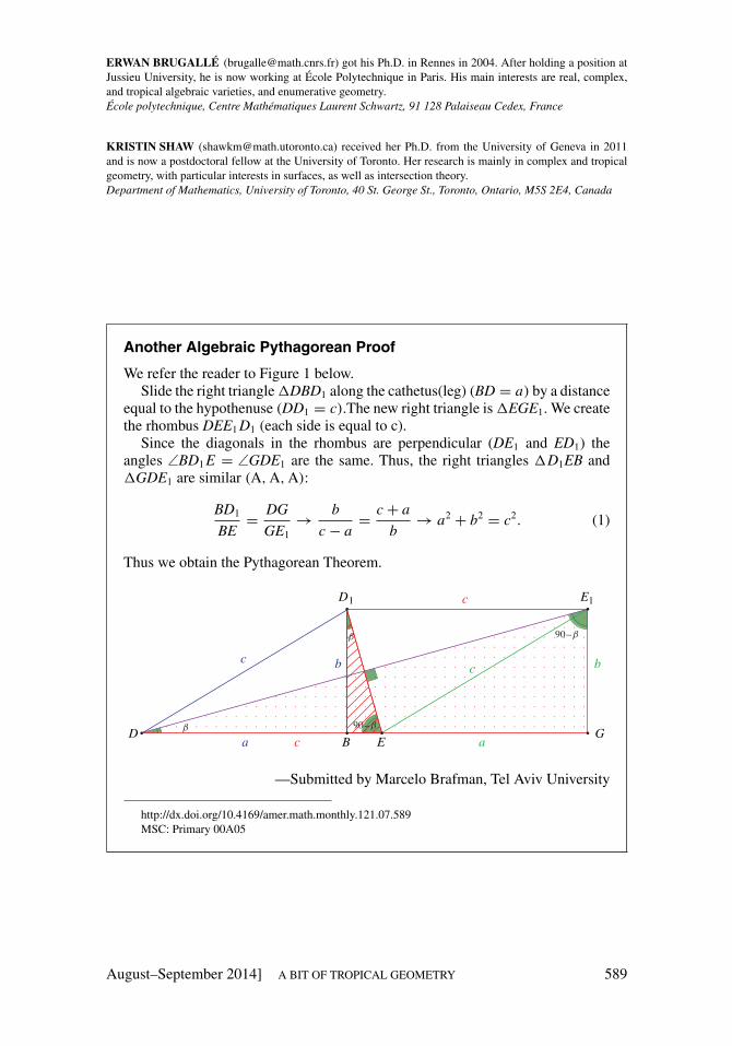
ERWAN BRUGALLE ([email protected]) got his Ph.D. in Rennes in 2004. After holding a position atJussieu University, he is now working at Ecole Polytechnique in Paris. His main interests are real, complex,and tropical algebraic varieties, and enumerative geometry.Ecole polytechnique, Centre Mathematiques Laurent Schwartz, 91 128 Palaiseau Cedex, France

KRISTIN SHAW ([email protected]) received her Ph.D. from the University of Geneva in 2011and is now a postdoctoral fellow at the University of Toronto. Her research is mainly in complex and tropicalgeometry, with particular interests in surfaces, as well as intersection theory.Department of Mathematics, University of Toronto, 40 St. George St., Toronto, Ontario, M5S 2E4, Canada

Another Algebraic Pythagorean Proof

We refer the reader to Figure 1 below.Slide the right triangle1DBD1 along the cathetus(leg) (BD = a) by a distance

equal to the hypothenuse (DD1 = c).The new right triangle is1EGE1. We createthe rhombus DEE1 D1 (each side is equal to c).

Since the diagonals in the rhombus are perpendicular (DE1 and ED1) theangles ∠BD1 E = ∠GDE1 are the same. Thus, the right triangles 1D1EB and1GDE1 are similar (A,A,A):

BD1

BE= DG

GE1→ b

c − a= c + a

b→ a2 + b2 = c2. (1)

Thus we obtain the Pythagorean Theorem.

. . . . . . . . . . . . . . . . . . . . . . . . . . . . . . . . . . . . . . . . . . .. . . . . . . . . . . . . . . . . . . . . . . . . . . . . . . . . . . . . . .

. . . . . . . . . . . . . . . . . . . . . . . . . . . . . . . . . . . .. . . . . . . . . . . . . . . . . . . . . . . . . . . . . . . .

. . . . . . . . . . . . . . . . . . . . . . . . . . . .. . . . . . . . . . . . . . . . . . . . . . . . .

. . . . . . . . . . . . . . . . . . . . .. . . . . . . . . . . . . . . . . .

. . . . . . . . . . . . . .. . . . . . . . . .

. . . . . . .. . .

Ba Ec a

cc

GD

D1 E1

b b

β

β 90–β

90–β

c

—Submitted by Marcelo Brafman, Tel Aviv University

http://dx.doi.org/10.4169/amer.math.monthly.121.07.589MSC: Primary 00A05





Four Quotient Set Gems

Bryan Brown, Michael Dairyko, Stephan Ramon Garcia,Bob Lutz, and Michael Someck

Abstract. Our aim in this note is to present four remarkable facts about quotient sets. Theseobservations seem to have been overlooked by the MONTHLY, despite its intense coverage ofquotient sets over the years.

INTRODUCTION. If A is a subset of the natural numbers N = {1, 2, . . .}, then welet R(A) = {a/a′ : a, a′ ∈ A} denote the corresponding quotient set (sometimes calleda ratio set). Our aim in this short note is to present four remarkable results, which seemto have been overlooked in the MONTHLY, despite its intense coverage of quotient setsover the years [3, 4, 5, 9, 10, 11, 14]. Some of these results are novel, while others haveappeared in print elsewhere but somehow remain largely unknown.

In what follows, we let A(x) = A ∩ [1, x] so that |A(x)| denotes the number ofelements in A which are ≤ x . The lower asymptotic density of A is the quantity

d(A) = lim infn→∞

|A(n)|

n,

which satisfies the obvious bounds 0 ≤ d(A) ≤ 1. We say that A is fractionally denseif the closure of R(A) in R equals [0,∞) (i.e., if R(A) is dense in [0,∞)).

Our four gems are as follows.

1. The set of all natural numbers whose base-b representation begins with the digit1 is fractionally dense for b = 2, 3, 4, but not for b ≥ 5.

2. For each δ ∈ [0, 12 ), there exists a set A ⊂ N with d(A) = δ that is not fraction-

ally dense. On the other hand, if d(A) ≥ 12 , then A must be fractionally dense

[15].

3. We can partition N into three sets, each of which is not fractionally dense. How-ever, such a partition is impossible using only two sets [2].

4. There are subsets of N that contain arbitrarily long arithmetic progressions, yetthat are not fractionally dense. On the other hand, there exist fractionally densesets that have no arithmetic progressions of length ≥ 3.

BASE-b REPRESENTATIONS. In [5, Example 19], it was shown that the set

A = {1} ∪ {10, 11, 12, 13, 14, 15, 16, 17, 18, 19} ∪ {100, 101, . . .} ∪ · · ·

of all natural numbers whose base-10 representation begins with the digit 1 is notfractionally dense. This occurs despite the fact that d(A) = 1

9 , so that a positive pro-portion of the natural numbers belongs to A. The consideration of other bases revealsthe following gem.

http://dx.doi.org/10.4169/amer.math.monthly.121.07.590MSC: Primary 11A99, Secondary 11B99; 11A16



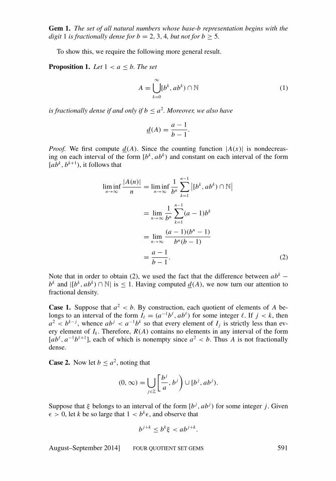
Gem 1. The set of all natural numbers whose base-b representation begins with thedigit 1 is fractionally dense for b = 2, 3, 4, but not for b ≥ 5.

To show this, we require the following more general result.

Proposition 1. Let 1 < a ≤ b. The set

A =∞⋃

k=0

[bk, abk) ∩ N (1)

is fractionally dense if and only if b ≤ a2. Moreover, we also have

d(A) =a − 1

b − 1.

Proof. We first compute d(A). Since the counting function |A(x)| is nondecreas-ing on each interval of the form [bk, abk) and constant on each interval of the form[abk, bk+1), it follows that

lim infn→∞

|A(n)|

n= lim inf

n→∞

1

bn

n−1∑k=1

∣∣[bk, abk) ∩ N∣∣

= limn→∞

1

bn

n−1∑k=1

(a − 1)bk

= limn→∞

(a − 1)(bn− 1)

bn(b − 1)

=a − 1

b − 1. (2)

Note that in order to obtain (2), we used the fact that the difference between abk−

bk and |[bk, abk) ∩ N| is ≤ 1. Having computed d(A), we now turn our attention tofractional density.

Case 1. Suppose that a2 < b. By construction, each quotient of elements of A be-longs to an interval of the form I` = (a−1b`, ab`) for some integer `. If j < k, thena2 < bk− j , whence ab j < a−1bk so that every element of I j is strictly less than ev-ery element of Ik . Therefore, R(A) contains no elements in any interval of the form[ab`, a−1b`+1], each of which is nonempty since a2 < b. Thus A is not fractionallydense.

Case 2. Now let b ≤ a2, noting that

(0,∞) =⋃j∈Z

[b j

a, b j

)∪ [b j , ab j ).

Suppose that ξ belongs to an interval of the form [b j , ab j ) for some integer j . Givenε > 0, let k be so large that 1 < bkε, and observe that

b j+k≤ bkξ < ab j+k .

August–September 2014] FOUR QUOTIENT SET GEMS 591

Let ` be the unique natural number satisfying

b j+k+ ` ≤ bkξ < b j+k

+ `+ 1 (3)

and

0 ≤ ` ≤ (a − 1)b j+k− 1. (4)

From (3), we find that

0 ≤ bkξ − (b j+k+ `) < 1,

from which it follows that

0 ≤ ξ −b j+k+ `

bk< ε.

Since (4) ensures that b j+k+ ` belongs to the interval [b j+k, ab j+k), we conclude

that (b j+k+ `)/bk belongs to R(A). A similar argument applies if ξ belongs to an

interval of the form [ b j

a , b j ). Putting this all together, we conclude that A is fractionallydense.

To see that Gem 1 follows from the preceding proposition, observe that if a = 2and b ≥ 2 is an integer, then the set A defined by (1) is precisely the set of all naturalnumbers whose base-b representation begins with the digit 1. The inequality b ≤ a2

holds precisely for the bases b = 2, 3, 4 and fails for all b ≥ 5.

CRITICAL DENSITY. Having seen that there exist sets that are not fractionallydense, yet whose lower asymptotic density is positive, it is natural to ask whetherthere exists a critical value 0 < κ ≤ 1 such that κ ≤ d(A) ensures that A is fractionallydense. The following gem establishes the existence of such a critical density, namelyκ = 1

2 .

Gem 2. If d(A) ≥ 12 , then A is fractionally dense. On the other hand, if 0 ≤ δ < 1

2 ,then there exists a subset A ⊂ N with d(A) = δ that is not fractionally dense.

Establishing this result will take some work, although we are now in a positionto prove the second statement (originally obtained by Strauch and Toth [15, Thm. 1]and by Harman [8, p. 167] using slightly different methods). If 0 ≤ δ < 1

2 , then wemay write δ = 1

2+ε where ε > 0. Now let a = 1 + ε

2 and b = 1 + ε + 12ε

2 so that1 < a2 < b. For these parameters, Proposition 1 tells us that the set A defined by (1)satisfies d(A) = δ and fails to be fractionally dense. If δ = 0, then we note that the setA = {2n : n ∈ N} is not fractionally dense and has d(A) = 0.

Thus, we can construct sets having lower asymptotic density arbitrarily close to 12 ,

yet which fail to be fractionally dense. On the other hand, it is clear that fractionallydense sets with d(A) = 1

2 exist. Indeed, one such example is A = {2, 4, 6, . . .}. How-ever, the question of whether a non-fractionally dense set can have lower asymptoticdensity equal to the critical density 1

2 is much more difficult.In the late 1960s, Salat proposed an example of a set A ⊂ N that is not fractionally

dense and such that d(A) = 12 [12, p. 278]. However, Salat’s example was flawed, as


pointed out in the associated corrigendum [13]. In 1998, Strauch and Toth establisheda more general result [15, Thm. 2], which implies that a set satisfying d(A) ≥ 1

2 mustbe fractionally dense (fortunately, the lengthy corrigendum [16] to this paper does notaffect the result in question). For d(A) > 1

2 , the fractional density of A also followsfrom a sophisticated theorem in metric number theory [8, Thm. 6.6] (although Harmanwas kind enough to show us an elementary proof in this case). The proof below, whichcovers the critical case d(A) = 1

2 , is essentially due to Strauch and Toth.

Theorem 2. If d(A) ≥ 12 , then A is fractionally dense.

Proof. Let d(A) ≥ 12 and suppose toward a contradiction that 0 < α < β ≤ 1 and

R(A) ∩ (α, β) = ∅. Noting that A must be infinite, we enumerate the elements of Ain increasing order a1 < a2 < · · · . Let k be a natural number, which is so large thatkα > 1, and let 0 < θ < 1. For all m and n in N, let

J nm =

(αak(bθnc+m), α(ak(bθnc+m) + k)

).

For each n in N, we claim that the intervals

J n0 , J n

1 , . . . , J nn−bθnc−1, (αakn, βakn), (5)

used below in a delicate counting argument, are pairwise disjoint. Indeed, since the ai

are integers, it follows that

α(ak(bθnc+m) + k) ≤ α(ak(bθnc+m)+k) = α(ak(bθnc+m+1)),

so that the right endpoint of J nm is at most the left endpoint of J n

m+1. A similar argumentshows that the right endpoint of J n

n−bθnc−1 is at most αakn .Next, let n be so large that bθnc ≥ α

β−α. We claim that

J nm ⊆

(αak(bθnc+m), βak(bθnc+m)

)(6)

for each m = 0, 1, . . . , n − bθnc − 1. To see this, note that

kα

β − α≤ kbθnc ≤ akbθnc < akbθnc+m,

which implies that α(ak(bθnc+m) + k) ≤ βak(bθnc+m) so that (6) holds.Since (αan, βan) ∩ A = ∅ by assumption, it follows now that the intervals (5) are

contained in the complement [0,∞)\A. Letting B = N \ A, a naıve counting argu-ment gives

|B(βakn)| ≥((β − α)akn − 1

)+ (n − bθnc)(kα − 1).

Dividing through by βakn and taking limits superior yields

1− d(A) = lim supn→∞

|B(n)|

n

≥ lim supn→∞

|B(βakn)|

βakn


≥ lim supn→∞

((β − α)akn − 1

βakn+(n − bθnc)(kα − 1)

βakn

)≥β − α

β+ lim inf

n→∞

(n − bθnc)(kα − 1)

βakn

≥ 1−α

β+ (1− θ) lim inf

n→∞

αkn − n

βakn

≥ 1−α

β+ (1− θ)

(α

βlim inf

n→∞

kn

akn−

1

βklim sup

n→∞

kn

akn

)≥ 1−

α

β+ (1− θ)

(α

βd(A)−

1

βk

).

Taking the limit as θ → 0 and k →∞ and rearranging gives(1+

α

β

)d(A) ≤

α

β. (7)

If d(A) ≥ 12 , then the preceding inequality implies that β ≤ α, a contradiction.

The astute reader will note that we have actually shown that if (α, β) ∩ R(A) = ∅,then (7) must hold. In fact, with only a little more work, we can show that

d(A) ≤α

βmin

{d(A), 1− d(A)

}and d(A) ≤ 1− (β − α), where

d(A) = lim supn→∞

|A(n)|

n

denotes the upper asymptotic density of A [15, Thm. 2]. Moreover, it is also knownthat d(A)+ d(A) ≥ 1 implies that A is fractionally dense [15, p. 71].

PARTITIONS OF N. Clearly, N itself is fractionally dense since R(N) = Q ∩(0,∞), the set of positive rational numbers. An interesting question now presentsitself. If N is partitioned into a finite number of disjoint subsets, does one of thesesubsets have to be fractionally dense? The following result gives a complete answer tothis problem.

Gem 3. We can partition N into three sets, each of which is not fractionally dense.However, such a partition is impossible using only two sets.

This gem is due to Bukor, Salat, and Toth [2]. These three, along with P. Erdos,later generalized the second statement by showing that if the set A is presented asan increasing sequence a1 < a2 < · · · satisfying limn→∞ an+1/an = 1, then for eachB ⊆ A, either B or A\B is fractionally dense [1].

The proof of our third gem is contained in the following two results.

Proposition 3. There exist disjoint sets A, B,C ⊂ N, none of which are fractionallydense, such that N = A ∪ B ∪ C.


Proof. Let

A =∞⋃

k=0

[5k, 2 · 5k

)∩ N,

B =∞⋃

k=0

[2 · 5k, 3 · 5k

)∩ N,

and

C =∞⋃

k=0

[3 · 5k, 5 · 5k

)∩ N,

so that A, B, and C consist of those natural numbers whose base-5 expansions be-gin, respectively, with 1, with 2, and with 3 or 4. We consider only C here, for theremaining two cases are similar (in fact, the set A is already covered by Proposition1). Observe that each quotient of elements of C is contained in an interval of the formI` =

(35 5`, 5

3 5`)

for some integer `. If j < k, then every element of I j is strictly lessthan every element of Ik , since 5

3 · 5j < 3

5 · 5k holds if and only if 25

9 < 5k− j . Thus,R(C) ∩ [ 5

3 5`, 35 5`+1] = ∅ for any integer `.

Theorem 4. If A and B are disjoint sets such that N = A ∪ B, then at least one ofA, B is fractionally dense.

Proof. Without loss of generality, we may assume that both A and B are infinite.Suppose, toward a contradiction, that neither A nor B is fractionally dense. Thus, thereexists α, β > 1, and ε > 0 such that (α − ε, α + ε)∩ R(A) and (β − ε, β + ε)∩ R(B)are both empty. Now, let n0 ∈ N be such that

1+ α + β + 2αβ

n0< ε.

Since A and B are both infinite, there exists n > αβ(n0 + 1) such that n ∈ A andn + 1 ∈ B. If s = b n

αβc − 1 belongs to A, then setting t = bαsc yields

∣∣∣∣ ts − α∣∣∣∣ = ∣∣∣∣bαsc − αs

s

∣∣∣∣ < 1

s≤

1

n0< ε. (8)

Since (α − ε, α + ε) ∩ R(A) = ∅, we conclude that t belongs to B. Now, observe that∣∣∣∣n + 1

t− β

∣∣∣∣ = n + 1− βbαsc

t

<n + 1− β(αs − 1)

t

=1+ β + αβ + n − αβb n

αβc

t

<1+ β + 2αβ

t


≤1+ β + 2αβ

n0

< ε.

Hence, n+1t belongs to (β − ε, β + ε) ∩ R(B), which is a contradiction. Therefore, it

must be the case that s belongs to B.Assuming now that s = b n

αβc − 1 belongs to B, we now let t = bβsc. Proceeding

as in (8), we can show that | ts − β| < ε and hence that t belongs to A. Moreover,∣∣∣nt− α

∣∣∣ = ∣∣∣∣n − αbβsc

t

∣∣∣∣<

n − α(βs − 1)

t

=α + n − αβs

t

=α + n − αβ(b n

αβc − 1)

t

=α + αβ + (n − αβb n

αβc)

t

<α + 2αβ

n0

< ε.

Thus, nt belongs to (α − ε, α + ε)∩ R(A), a contradiction which implies that s belongs

to neither A nor B, an absurdity, since N = A ∪ B.

Although we might be tempted to postulate a relationship between Theorems 2 and4, lower asymptotic density has no bearing on the preceding result, since it is possibleto partition N into two subsets both having lower asymptotic density zero.

Proposition 5. There exist disjoint sets A, B ⊂ N such that N = A ∪ B, d(A) =d(B) = 0, and d(A) = d(B) = 1.

Proof. We require the Stolz–Cesaro Theorem [6], which tells us that if xn and yn aretwo increasing and unbounded sequences of real numbers, then

limn→∞

xn+1 − xn

yn+1 − yn= L =⇒ lim

n→∞

xn

yn= L .

Now put the first 1! natural numbers into A, then the next 2! into B, the next 3! into A,and so forth, yielding the sets

A = {1, 4, 5, 6, 7, 8, 9, 34, . . .}, B = {2, 3, 10, 11, 12, . . . , 32, 33, 154, 155, . . .}.

By construction, A ∩ B = ∅ and N = A ∪ B. Let xn =∑2n−1

k=1 k! and yn =∑2n

k=1 k!,observing that |A(xn)| = |A(yn)| =

∑nk=1(2k − 1)!. Since

|A(yn+1)| − |A(yn)|

yn+1 − yn=

(2n + 1)!

(2n + 2)!+ (2n + 1)!=

1

2n + 3→ 0


and

|A(xn+1)| − |A(xn)|

xn+1 − xn=

(2n + 1)!

(2n + 1)!+ (2n)!=

1

1+ 12n+1

→ 1,

it follows from the Stolz–Cesaro Theorem that d(A) = 0 and d(A) = 1. An analo-gous argument using xn =

∑2nk=1 k! and yn =

∑2n+1k=1 k! now reveals that d(B) = 0 and

d(B) = 1 as well.

ARITHMETIC PROGRESSIONS. Our final gem concerns arithmetic progressionsof natural numbers. Recall that an arithmetic progression with common difference band length n is a sequence of the form a, a + b, a + 2b, . . . , a + (n − 1)b. Subsetsof the natural numbers that contain arbitrarily long arithmetic progressions are oftenthought of as being “thick” or “dense” in some qualitative sense.

Gem 4. There exists a subset of N containing arbitrarily long arithmetic progressionsthat is not fractionally dense. On the other hand, there exists a fractionally dense setthat has no arithmetic progressions of length ≥ 3.

The first statement of Gem 4 has already been proven. Indeed, Proposition 1 pro-duces sets that are not fractionally dense and that contain arbitrarily long blocks ofconsecutive natural numbers. We therefore need only produce a fractionally dense sethaving no arithmetic progressions of length three (see also [9, Thm. 2]).

Proposition 6. The set A = {2 j : j ≥ 2} ∪ {3k : k ≥ 2} is fractionally dense and con-tains no arithmetic progressions of length three.

Proof. First, recall that Kronecker’s approximation theorem [7, Thm. 440] asserts thatif β > 0 is irrational, α ∈ R, and δ > 0, then there exist n,m ∈ N such that |nβ −α − m| < δ. Let ξ, ε > 0 and note that β = log2 3 > 0 is irrational. By the continuityof f (x) = 2x at log2 ξ , there exists δ > 0 such that

| log2 x − log2 ξ | < δ =⇒ |x − ξ | < ε. (9)

Kronecker’s theorem with β = log2 3 and α = log2 ξ now yields n,m ∈ N so that∣∣∣∣log2

(3n

2m

)− log2 ξ

∣∣∣∣ = |n log2 3− log2 ξ − m| < δ.

In light of (9), it follows that |3n/2m− ξ | < ε, whence A is fractionally dense.

We now show that A contains no arithmetic progressions of length three. Assume,toward a contradiction, that such an arithmetic progression exists. By the definition ofA, the first term in this progression is either a power of 2 or a power of 3. We considerboth cases separately, letting b denote the common difference in each progression.

Case 1. Suppose that 2 j , 2 j+ b, and 2 j

+ 2b belong to A. Since 2 j+ 2b is even and

belongs to A, it must be of the form 2k for some k > j , whence b = 2k−1− 2 j−1 is

even since j ≥ 2. Thus, 2 j+ b must also be of the form 2` for some ` > j so that

2` = 2 j+ b = 2 j

+ (2k−1− 2 j−1) = 2 j−1(2k− j

+ 1).

Upon dividing the preceding by 2 j−1 we obtain a contradiction.


Case 2. Now suppose that 3 j , 3 j+ b, 3 j

+ 2b is an arithmetic progression in A oflength three that begins with 3 j . In this case, 3 j

+ 2b is odd and hence must be of theform 3k for some k > j . Therefore,

b =3k− 3 j

2= 3 j (3

k− j− 1)

2,

so that the second term 3 j+ b in our progression is divisible by 3 j . Thus, 3 j

+ b = 3`

for some ` > j , from which it follows that

3` = 3 j+ b = 3 j

+ 3 j (3k− j− 1)

2.

Since this implies that 2 · 3`− j= 2+ (3k− j

− 1), which is inconsistent modulo 3, weconclude that A has no arithmetic progressions of length three.

ACKNOWLEDGMENT. Partially supported by National Science Foundation Grant DMS-1001614.

REFERENCES

1. J. Bukor, P. Erdos, T. Salat, J. T. Toth, Remarks on the (R)-density of sets of numbers, II, Math. Slovaca47 (1997) 517–256.

2. J. Bukor, T. Salat, J. T. Toth, Remarks on R-density of sets of numbers, Tatra Mt. Math. Publ. 11 (1997)159–165.

3. J. Bukor, J. T. Toth, On accumulation points of ratio sets of positive integers, Amer. Math. Monthly 103(1996) 502–504.

4. S. R. Garcia, Quotients of Gaussian primes, Amer. Math. Monthly 120 (2013) 851–853.5. S. R. Garcia, V. Selhorst-Jones, D. E. Poore, N. Simon, Quotient sets and Diophantine equations, Amer.

Math. Monthly 118 (2011) 704–711.6. R. Gelca, T. Andreescu, Putnam and Beyond. Springer, New York, 2007.7. G. H. Hardy, E. M. Wright, An Introduction to the Theory of Numbers. Sixth edition. Oxford University

Press, Oxford, 2008.8. G. Harman, Metric Number Theory. London Mathematical Society Monographs. New Series. Vol. 18.

Clarendon Press Oxford University Press, New York, 1998.9. S. Hedman, D. Rose, Light subsets of N with dense quotient sets, Amer. Math. Monthly 116 (2009)

635–641.10. D. Hobby, D. M. Silberger, Quotients of primes, Amer. Math. Monthly 100 (1993) 50–52.11. A. Nowicki, Editor’s endnotes, Amer. Math. Monthly 117 (2010) 755–756.12. T. Salat, On ratio sets of sets of natural numbers, Acta Arith. 15 (1969) 273–278.13. , Corrigendum to the paper “On ratio sets of sets of natural numbers,” Acta Arith. 16 (1970) 103.14. P. Starni, Answer to two questions concerning quotients of primes, Amer. Math. Monthly 102 (1995)

347–349.15. O. Strauch, J. T. Toth, Asymptotic density of A ⊂ N and density of the ratio set R(A), Acta Arith. 87

(1998) 67–78.16. , Corrigendum to Theorem 5 of the paper: “Asymptotic density of A ⊂ N and density of the ratio

set R(A),” Acta Arith. 103 (2002) 191–200.

BRYAN BROWN is a junior at Pomona College majoring in mathematics and minoring in computer [email protected]

MICHAEL DAIRYKO graduated from Pomona College in 2013 with a degree in mathematics and is cur-rently a Ph.D. student at Iowa State University. He hopes to become a professor at a small liberal arts collegewhere the climate is warm. When not “mathing,” he enjoys the outdoors, socializing with friends, and playingwater polo.Department of Mathematics, Iowa State University, 396 Carver Hall, Ames, IA [email protected]




STEPHAN RAMON GARCIA grew up in San Jose, California before attending U.C. Berkeley for his B.A.and Ph.D. After graduating, he worked at U.C. Santa Barbara for several years before moving to PomonaCollege in 2006. He has earned three NSF research grants and five teaching awards from three different in-stitutions. He is the author of fifty research articles in operator theory, complex analysis, matrix analysis, andnumber theory. http://pages.pomona.edu/~sg064747Department of Mathematics, Pomona College, Claremont, CA [email protected]

BOB LUTZ is a recent graduate from Pomona College and a Ph.D. student in mathematics at the Universityof Michigan. An ardent gourmand and sometimes-author, he aspires to teach at a liberal arts college one day,but is tempted by the more stable prospect of a career in food blogging.Department of Mathematics, University of Michigan, 2074 East Hall, 530 Church Street,Ann Arbor, MI [email protected]

MICHAEL SOMECK is a junior mathematics and philosophy double major at Pomona College, currentlyspending a year abroad at the University of Oxford. He is interested in the ways in which mathematiciansand philosophers often use the same tool, logic, to solve completely different problems. In his free time, heenjoys traveling, spending time with friends, reading a good book, or relaxing at a beach in his hometown ofSan [email protected]

100 Years ago this Month in The American Mathematical MonthlyEdited by Vadim Ponomarenko

That there has been and still is an unrest among thoughtful high school teachersof mathematics is manifest. This problem certainly exists: How are we to adaptthe courses in algebra and geometry to the experiences of high school students,in order that these may contribute to their broader development in both a culturaland a practical way? On the one hand we have the student who is preparing forthe university and on the other hand the student whose school life ends with thehigh school or who, going on to the university, will not continue the subject ofmathematics. The one who would solve this problem must have these two classesin view, and the solution for the one must be the solution for the other since itis only in the largest schools that distinction can be made by having separateclasses, even if it were advisable.

—Excerpted from “Miscellaneous Questions” 21 (1914), 239.


http://pages.pomona.edu/~sg064747




Blind-friendly von Neumann’s Heads or Tails

Vinıcius G. Pereira de Sa and Celina M. H. de Figueiredo

Abstract. The toss of a coin is usually regarded as the epitome of randomness, and hasbeen used for ages as a means to resolve disputes in a simple, fair way. Perhaps as ancientas consulting objects such as coins and dice is the art of maliciously biasing them in orderto unbalance their outcomes. However, it is possible to employ a biased device to produceequiprobable results in a number of ways, the most famous of which is the method suggestedby von Neumann back in 1951. This paper addresses how to extract uniformly distributed bitsof information from a nonuniform source. We study some probabilities related to biased diceand coins, culminating in an interesting variation of von Neumann’s mechanism that can beemployed in a more restricted setting where the actual results of the coin tosses are not knownto the contestants.

1. INTRODUCTION. Estimating probabilities is one of those tasks at which thehuman brain seems to be not very good. Conditional probabilities, in particular, fre-quently defy—and defeat—one’s intuition, from the uninitiated to the specialist. Thisexplains to a certain extent why people lose money gambling and on similar activ-ities. Led astray by instinct, the inadvertent player overlooks probabilistic subtletiesand misestimates the odds.

In this paper, we study some probabilities that may be rather counterintuitive. Al-though our results were formulated in the context of games between two opponents,they could as well have been framed in terms of the general engineering problem ofconverting biased randomness into unbiased randomness, a fascinating subject withplenty of literature available (see, for instance, [3, 4, 10, 11, 13, 14]).

In Section 2, we describe a game where the winning chances depend on the fairnessof a die with n ≥ 2 sides in a nontrivial way. Indeed, even knowing beforehand theexact probability associated to each side of the die, it may not be so easy to decide,between two seemingly equivalent strategies, which one is the most advantageous.Still, it is possible to show that one of the strategies is never worse than the other,no matter the bias or the number of sides of the die. We then look at some specialcases. Particularly for n = 2, we derive the winning chances as a function of the bias,showing how to maximize the probability that a given player wins.

In Section 3, we consider the following questions regarding three independent andidentically distributed (iid) random variables A, B, and C . Are the events C = B andB 6= A always independent? When, and to which extent, may (the knowledge of) theformer affect (the probability of) the latter? The answers to these questions are closelyrelated to the results in Section 2.

Finally, in Section 4, we leverage the results from the previous sections into a vari-ation of von Neumann’s method of playing a fair heads or tails with a biased coin.Numerous improvements on von Neumann’s original idea have been studied over thedecades ([1, 7, 9, 12], to mention but a few). Our method handles, however, an extrarestriction: The players do not know the actual result of each coin toss; instead, theyare only aware of whether each toss produced the same result as the previous one alonga sequence of independent tosses.

http://dx.doi.org/10.4169/amer.math.monthly.121.07.600MSC: Primary 60C05, Secondary 60G40



2. A TRIPLE OR TWO STRAIGHT DOUBLES? In this section, we discuss avery simple dice game, not only for its own sake, but also for the useful inequality weobtain from it.

Consider a die with n ≥ 2 sides. We propose a game where each player must choosebetween two strategies: playing for a “triple”, or two “consecutive doubles”. In the for-mer strategy, the player throws the die three times, scoring a point if the die producesthree identical results. In the latter, the player throws the die four times, scoring a pointif the results after the first and the second throws match one another and the third andfourth results also match one another. After repeating their sequences of throws a pre-viously arranged number of times, the player with more points wins the game.

We might think that both strategies are equally good (or equally terrible, dependingon how big n is). Indeed, when playing for a triple, there are two critical momentsat which the player needs to be lucky: at the second throw, whose result is requiredto match the first one; and at the third throw, which is also required to match theother two. When playing for two doubles in a row, there are also two such criticalmoments: at the second throw, when the player wants the die to match the result thatjust preceded it, and again at the fourth throw, for the same reason. In spite of theirapparent equivalence, the odds for both strategies are not always as good, and howmore advantageous one strategy is depends on the fairness of the die.

In order to get some intuition, suppose our die is strongly biased towards one partic-ular outcome (say it results in a 1 in 90% of the throws). What difference does it make,now, to play for a triple or two straight doubles? When playing for a triple, we haveonly three chances of “going wrong”, that is, of throwing the die and obtaining some-thing other than 1. (Of course, it is possible that some other-than-1 outcome appearsthree times in a row, but that is definitely unlikely.) On the other hand, when playingfor two straight doubles, we have in practice four chances of “going wrong”, since anyother-than-1 outcome that ends up occurring will most likely remain unmatched. Nowwe proceed to a more formal discussion.

Claim 1. If A, B, C, and D are iid discrete random variables, then

Pr{A = B ∧ C = D} ≤ Pr{A = B = C}.

Proof. Let � be the range of possible values of A, B, C , and D. For i ∈ �, let pi be theprobability Pr{A = i} = Pr{B = i} = Pr{C = i} = Pr{D = i} that a given variabletakes value i . Let E2,2 denote the event that A = B and C = D, and let E3 denote theevent that A = B = C . Since the variables are independent, we can write

Pr{E2,2} =

(∑i∈�

p2i

)2

(1)

and

Pr{E3} =

∑i∈�

p3i . (2)

We now show that Pr{E2,2} ≤ Pr{E3}. Inspired by its use in [5], we recall the Cauchyinequality [2, p. 373] (∑

i∈�

xi yi

)2

≤

(∑i∈�

x2i

)(∑i∈�

y2i

).

August–September 2014] 601

Setting xi = p3/2i and yi = p1/2

i , we obtain(∑i∈�

p2i

)2

≤

(∑i∈�

p3i

)(∑i∈�

pi

)=

∑i∈�

p3i

as desired.

As a consequence, the probability of obtaining a triple in three throws of a die isnever less than the probability of obtaining two straight doubles in four throws of thatdie. It should now be clear that equality must not be taken for granted. We look at somespecial cases.

From now on, let A, B, C , and D be specifically the results of four consecutivethrows of an n-sided die; that is, iid random variables defined by selections on thesample space � = {1, . . . , n}. We denote by pi the probability that i is the resultobtained by throwing that die, for i ∈ �.

Perfectly fair dice. Consider the case where pi = 1/n for all i ∈ �; that is, our die is“perfectly fair”. In this situation, equations (1) and (2) yield

Pr{E3} = Pr{E2,2} =1

n2,

and therefore both players have the same probability of winning the game. As a matterof fact, it is a simple exercise to show that Claim 1 holds with equality if, and onlyif, either the random variables are uniformly distributed over a subset of their samplespace, or one of the possible outcomes occur with probability 1.

Perfectly loaded dice. Suppose the die was manufactured in such a way that the sameside always ends upwards after a throw, e.g. p1 = 1, and pi = 0 for i ∈ {2, . . . , n}. Ofcourse, both strategies will score a point at each and every sequence of throws, andthe game will almost certainly end in a draw. As in the perfectly fair case, there is nopreferable strategy.

Coins. We now focus on the case n = 2 and call our die a coin. We are interested in thefunction d : [0, 1]→ [0, 1] that quantifies the advantage d(p) = Pr{E3} − Pr{E2,2} ofplaying for a triple when the probability of our coin landing heads is p. By makingp1 = p and p2 = 1− p in (1) and (2), we obtain

d(p) =[

p3+ (1− p)3

]−[

p2+ (1− p)2

]2

= −4p4+ 8p3

− 5p2+ p.

It is now easy to see (Figure 1) that d has minimum value 0 at p ∈ {0, 0.5, 1} as ex-pected, and maximum value 0.0625 at p = 1/2± 1/(2

√2) ≈ 0.5± 0.3536. In other

words, 6.25% is the largest possible probabilistic advantage that can be obtained inthis game.1 This is achieved by the player who plays for a triple when the probabilityof the coin landing heads (or tails, by symmetry) is approximately 85.36%.

1Should a winning margin of 6.25% appear to be rather small, compare it with the casino’s winning marginof 5.26% in American roulette, and of only 2.70% in European roulette. Yet we do not see casinos goingbankrupt too often!


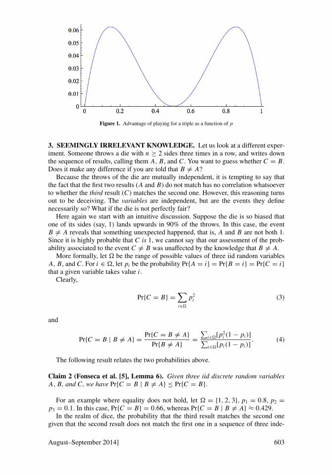
Figure 1. Advantage of playing for a triple as a function of p

3. SEEMINGLY IRRELEVANT KNOWLEDGE. Let us look at a different exper-iment. Someone throws a die with n ≥ 2 sides three times in a row, and writes downthe sequence of results, calling them A, B, and C . You want to guess whether C = B.Does it make any difference if you are told that B 6= A?

Because the throws of the die are mutually independent, it is tempting to say thatthe fact that the first two results (A and B) do not match has no correlation whatsoeverto whether the third result (C) matches the second one. However, this reasoning turnsout to be deceiving. The variables are independent, but are the events they definenecessarily so? What if the die is not perfectly fair?

Here again we start with an intuitive discussion. Suppose the die is so biased thatone of its sides (say, 1) lands upwards in 90% of the throws. In this case, the eventB 6= A reveals that something unexpected happened, that is, A and B are not both 1.Since it is highly probable that C is 1, we cannot say that our assessment of the prob-ability associated to the event C 6= B was unaffected by the knowledge that B 6= A.

More formally, let � be the range of possible values of three iid random variablesA, B, and C . For i ∈ �, let pi be the probability Pr{A = i} = Pr{B = i} = Pr{C = i}that a given variable takes value i .

Clearly,

Pr{C = B} =∑i∈�

p2i (3)

and

Pr{C = B | B 6= A} =Pr{C = B 6= A}

Pr{B 6= A}=

∑i∈�[p2

i (1− pi )]∑i∈�[pi (1− pi )]

. (4)

The following result relates the two probabilities above.

Claim 2 (Fonseca et al. [5], Lemma 6). Given three iid discrete random variablesA, B, and C, we have Pr{C = B | B 6= A} ≤ Pr{C = B}.

For an example where equality does not hold, let � = {1, 2, 3}, p1 = 0.8, p2 =

p3 = 0.1. In this case, Pr{C = B} = 0.66, whereas Pr{C = B | B 6= A} ≈ 0.429.In the realm of dice, the probability that the third result matches the second one

given that the second result does not match the first one in a sequence of three inde-


pendent throws of a die is less than or equal to the unconditional probability that thethird result matches the second one.

Perfectly fair dice. By replacing pi with 1/n in equations (3) and (4), it is straight-forward to verify that both probabilities are equal to 1/n. In other words, if the die isfair, then the probability of having a match between the third and the second results isnot at all affected by the fact that the second throw and the first one do not match. Theevents are in this case independent.

Perfectly loaded dice. If the die always lands with the same side upwards, then itis impossible that two throws have different outcomes. Our comparison here is thenmeaningless.

Coins. When n = 2, the unconditional probability that two tosses of the coin yield thesame result is clearly

Pr{C = B} = p21 + p2

2 = p2+ (1− p)2

= 2p2− 2p + 1, (5)

where p denotes, without loss of generality, the probability of heads. Such a probabil-ity has minimum value 0.5 at p = 0.5 (i.e., a fair coin).

On the other hand, the conditional probability we are interested in is obtained fromequation (4) and translates to

Pr{C = B | B 6= A} =p2(1− p)+ (1− p)2 p

2p − 2p2

=p − p2

2p − 2p2

= 0.5,

regardless of p (of course, provided p is not 0 or 1).A simpler way of seeing this is to note that, given that the first two coins came up

differently, the second coin is uniformly distributed over heads and tails. Thus, theprobability that the third coin results the same as the second is 0.5p + 0.5(1− p) =

0.5.

This interesting result, which motivates the whole next section, is summarized inthe corollary below. We recall that a Bernoulli random variable is such that it takesvalue 1 with “success probability” p and value 0 with “failure probability” 1− p.

Corollary 3. Given three independent Bernoulli random variables A, B, and C withsuccess probability 0 < p < 1, we have Pr{C = B | B 6= A} = 0.5 regardless of p.

4. HAND CLAPS AND WHISTLES. The idea of playing a fair heads or tails witha biased coin2 is attributed to von Neumann [8] as follows. The coin is tossed twicein a row. The first player wins if the outcome is a heads-tails sequence, whereas thesecond player wins with a tails-heads sequence. If two identical results are obtained,another turn of two coin tosses starts from scratch. The probability of winning thegame at a certain turn is identical for both players, namely p(1− p), where p is the

2In spite of the numerous references to such entities over the centuries, some recent evidence seems to showthat there is no such thing as a biased coin that is caught by the hand (i.e., the coin is allowed to spin in the air,but not to bounce). See [6] for finding out why the biased coin may be considered the unicorn of probabilitytheory.


probability that a coin toss results heads. Thus, the probability that some player wins ata certain turn is q = 2p(1− p), and the number of turns until the game has a winner isa geometric random variable X whose expectation is E{X} = 1/q = 1/(2(p − p2)).Since each turn comprises exactly two coin tosses, the expected number of tosses untila player wins using von Neumann’s method is 2E{X} = 1/(p − p2).

Now suppose we have a situation where the coin is concealed, that is, the contestantsare not able to see the outcome of each toss. Instead, they can only figure out, after eachtoss, whether the result happened to match the one that just preceded it, which we referto as the base result. For the sake of illustration, consider that the coin is tossed by atrusted third party who claps hands each time the coin toss results the same as in theprevious toss, and who whistles otherwise. Only after the very first toss (the initialtoss, in each game), no sound is produced, since there is no base result to comparewith. We want to assure fairness, and we certainly cannot use von Neumann’s originalmethod, since the actual coin results are not known to the players.

We first discuss wrong ways of trying to obtain a fair game.

Unsuccessful attempts at fairness. In the proposed setting, the players cannot see theactual results, but they hear something after each toss3: a hand clap (Cl) or a whistle(Wh). Then why not simply regard a hand clap as heads, a whistle as tails, and playthe good old heads or tails? In other words, after the initial toss, toss the coin exactlyonce more. Player 1 wins with a hand clap, Player 2 wins with a whistle. Of coursewe can play such a game, but should not expect it to be fair if the coin itself is notfair. Indeed, the greater the coin bias, the greater the advantage of playing for a handclap. Formally, if p is the probability that the coin lands heads, then the probabilitythat Player 1 wins is equal to the probability that two independent tosses of the coinyield the same result, namely p2

+ (1− p)2= 2p2

− 2p + 1, whose minimum value0.5 is obtained at p = 0.5, as in (5).

Aiming at neutralizing the coin bias, a second, natural attempt is to use a straight-forward translation of von Neumann’s idea based on the perceived sounds. After theinitial toss, which sets the first base value, the coin is tossed twice in a row. Player1 wins with a Cl-Wh sequence, Player 2 wins with a Wh-Cl sequence. If any othersequence occurs, the game proceeds with another turn of two coin tosses. Is the gamenow fair, regardless of the coin bias? We show that it is not, except again if p = 0.5.

To calculate the probability P1 that Player 1 wins the game, let F H and F T denotethe events where the initial toss results heads (H) or tails (T), respectively, so that

P1 = Pr{P1 | F H} · Pr{F H

} + Pr{P1 | F T} · Pr{F T

}

by the law of total probability. By letting P H1 = Pr{P1 | F H

} and PT1 = Pr{P1 | F T

},we can write

P1 = P H1 · p + PT

1 · (1− p). (6)

We now obtain P H1 conditioned on the results of the two coin tosses that followed

the initial toss (whose result was heads, by definition):

• [base H] H-H—this sequence yields two hand claps, no player wins yet, and theprobability that Player 1 eventually wins is still P H

1 due to the memorylessness ofthe process, which now starts over with a new turn of two tosses still having headsas base value;

3Except for the initial toss, as mentioned above.


• [base H] H-T—this gives a Cl-Wh sequence, and victory is awarded to Player 1;• [base H] T-H—we have two whistles and no winner, hence the probability of Player

1 winning is still P H1 , as in the case H-H;

• [base H] T-T—a whistle followed by a hand clap: victory goes straight to Player 2.

Using again the law of total probability, we can write

P H1 =

∑S∈S

Pr{P H1 | S} · Pr{S}

= P H1 · p2

+ 1 · p(1− p)+ P H1 · (1− p)p + 0 · (1− p)2,

where S = {H-H, H-T, T-H, T-T} is the set of events associated to the two coin tossesthat follow the initial toss, as mentioned above. After some easy manipulations, weobtain

P H1 = p. (7)

An analogous argument shows that

PT1 = 1− p. (8)

By plugging (7) and (8) into (6), we obtain P1 = p2+ (1− p)2

= 2p2− 2p + 1.

This is again the same expression as in (5), which has minimum value 0.5 at p = 0.5.In short, the game is only fair when the coin itself is fair.

Before proceeding, it is interesting to notice that here—unlike the coin game pro-posed in Section 2, where a probability of heads around 0.5 ± 0.3536 would maxi-mize a player’s winning odds—the greater the coin bias, the greater the probabilitythat Cl-Wh wins over Wh-Cl, in spite of the apparent symmetry of both strategies.We could try this game against an inadvertent opponent (perhaps someone who er-roneously regards it as being equivalent to von Neumann’s method). However, us-ing a similar reasoning as in the calculation of P1, we see that the expected numberof tosses before the game finishes (disregarding the initial toss) is 1/(p − p2), as invon Neumann’s method. This fact cannot be disregarded. For example, when the coinis so biased that p = 0.999, though the Cl-Wh player has a winning probability of98.02%, the coin needs to be tossed 1001 times on average before the game has awinner!

In the next section, we look into a variation that successfully shields the playersfrom whatever bias the concealed coin might have (provided both sides appear withnon-zero probability).

Fair game with a concealed biased coin. We want to devise a coin game with thefollowing properties:

1. the coin is possibly biased, yet the exact bias is unknown to the players;2. both players have equal chances of winning;3. the actual coin results are not revealed, but it is possible to infer whether any two

consecutive coin tosses yielded the same result.

The two first conditions are the usual ones. Ideally, we would like to cope with thethird, new condition without incurring any increase in the expected duration of thegame.


First, let us consider the natural solution of tossing the coin four times, consideringthe sounds X and Y produced after the second and fourth tosses, respectively. Player1 wins with a Cl-Wh sequence, Player 2 wins with Wh-Cl, and the other possiblesequences are discarded, triggering four fresh tosses of the coin. By doing so, X andY are clearly independent, and this approach corresponds exactly to von Neumann’sidea, therefore assuring a fair game. The drawback is that it may take twice as long.

Now consider the following variation. The main action consists of tossing the cointwo consecutive times, whose results we call respectively A and B, constituting a turn.If a whistle is heard after the second toss (meaning B 6= A), then a third coin toss—whose result we call C—will decide the game. Player 1 wins if C 6= B (indicated bythe subsequent whistle), Player 2 wins if C = B (indicated by the subsequent handclap). On the other hand, if the sound alert after the second coin toss is a hand clap(meaning B = A), then the game continues with a fresh turn of two coin tosses that willset the values of A and B from scratch, configuring a perfectly memoryless process.Note that an initial toss that would set a base value prior to the first turn is not evennecessary here, since the players only care about sound alerts that come with evenparity (after the second, fourth, sixth tosses, etc.) until a whistle with even parity isheard for the first time. When it eventually happens, a single, decisive extra toss closesthe game.

Theorem 4. The proposed coin game, where Player 1 wins with a whistle of evenparity immediately followed by another whistle, and Player 2 wins with a whistle ofeven parity immediately followed by a hand clap, is a perfectly fair game, no matterthe probability of heads 0 < p < 1 of the employed coin.

Proof. Let A and B be the results of the two coin tosses that preceded the first whistlewith even parity. That very whistle indicates B 6= A. The next coin toss, whose resultwe call C , will decide the game in Player 1’s favor if C 6= B, and in Player 2’s favorif C = B. Using a simple (tails → 0, heads → 1) mapping, those three results areclearly independent Bernoulli random variables with success probability p. Thus, byCorollary 3, both players have identical probabilities

Pr{C 6= B | B 6= A} = Pr{C = B | B 6= A} = 0.5

of winning the game.

As for the expected number of tosses, notice that the event that a whistle is heardafter the second toss of a turn corresponds to the event that the two consecutive tossesof that turn produces either a H-T or a T-H sequence; hence, it occurs with probability2p(1− p). The number of turns before the game finishes is therefore a geometric ran-dom variable X , whose expectation is E{X} = 1/(2p(1− p)), plus one (correspond-ing to the final, decisive toss). Thus, the expected number of tosses in the game is

2 · E{X} + 1 =1

p − p2+ 1, (9)

which is only one coin toss greater than in the original von Neumann’s method.It is interesting to observe that, if in an attempt to reduce its expected duration, we

decided the game right after the first whistle regardless of its parity, then two unfortu-nate consequences would ensue:


(i) the intended “improvement” would not decrease the expected length of thegame at all; and, most importantly,

(ii) we would not be able to assure the fairness of the game anymore!

To show (i), let F H (and, respectively, F T ) denote the event that the first coin tossin the game yields heads (respectively, tails), and let Y be the random variable corre-sponding to the number of tosses before the first whistle is heard. Using conditional ex-pectations, we can write the overall expected number of tosses in the modified game as

1+ E{Y } = 1+ E{Y | F H} · Pr{F H

} + E{Y | F T} · Pr{F T

}

= 1+

(1+

1

1− p

)· p +

(1+

1

p

)· (1− p)

= 1+1

p − p2,

which is exactly the same as in (9).To show (ii), we argue that Player 1—who wins the game if the sound after the first

whistle is another whistle—will win the game exactly if:

• the first coin toss yields H, and the toss immediately after the first occurrence ofT (which produces the first whistle of the game) yields H (producing the secondwhistle in a row); or, analogously,

• the first coin toss yields T, and the toss immediately after the first occurrence of Hyields T.

Thus, the probability that Player 1 wins the game is p2+ (1− p)2

= 2p2− 2p + 1,

the same function of p seen in (5)—which has minimum value 0.5 exactly at p =0.5—yet again.

ACKNOWLEDGEMENTS. The “triple or two straight doubles” question was proposed to us by GuilhermeDias da Fonseca when he was studying randomized data structures. We are also grateful to Alexandre Stauffer,to Luiz Henrique de Figueiredo, and to the anonymous referees for the numerous valuable suggestions.

REFERENCES

1. M. Blum, Independent unbiased coin flips from a correlated biased source: a finite state Markov chain,Combinatorica 6 (1986) 97–108.

2. A. Cauchy, Oeuvres 2, III (1821).3. B. Chor, O. Goldreich, Unbiased bits from sources of weak randomness and probabilistic communication

complexity, in Proc. 26th IEEE Symp. on Foundations of Computer Science (1985) 429–442.4. P. Elias, The efficient construction of an unbiased random sequence, The Annals of Mathematical Statis-

tics 43 (1972) 865–870.5. G. D. da Fonseca, C. M. H. de Figueiredo, P. C. P. Carvalho, Kinetic hanger, Information Processing

Letters 89 (2004) 151–157.6. A. Gelman, D. Nolan, You can load a die, but you can’t bias a coin, The American Statistician 56 (2002)

308–311.7. W. Hoeffding, G. Simons, Unbiased coin tossing with a biased coin, The Annals of Mathematical Statis-

tics 41 (1970) 341–352.8. J. von Neumann, Various techniques used in connection with random digits, J. Res. National Bureau of

Standards 12 (1951) 36–38.9. Y. Peres, Iterating von Neumann’s procedure for extracting random bits, The Annals of Statistics 20

(1992) 590–597.10. P. A. Samuelson, Constructing an unbiased random sequence, Journal of the American Statistical Asso-

ciation 63 (1968) 1526–1527.


11. A. Srinivasan, D. Zuckerman, Computing with very weak random sources, SIAM Journal on Computing28 (1999) 1433–1459.

12. Q. F. Stout, B. Warren, Tree algorithms for unbiased coin tossing with a biased coin, The Annals ofProbability 12 (1984) 212–222.

13. S. Vembu, S. Verdu, Generating random bits from an arbitrary source: fundamental limits, IEEE Trans-actions on Information Theory 41 (1995) 1322–1332.

14. D. Zuckerman, Simulating BPP using a general weak random source, in Proc. 32nd IEEE Symp. onFoundations of Computer Science (1991) 79–89.

VINICIUS GUSMAO PEREIRA DE SA received his D.Sc. degree from Universidade Federal do Rio deJaneiro, where he is currently an associate professor. When he is neither working with combinatorics or pro-gramming computers, he can be seen bicycling or trying to play the piano.Departamento de Ciencia da Computacao, UFRJ, [email protected]

CELINA MIRAGLIA HERRERA DE FIGUEIREDO is a full professor at the Systems Engineering andComputer Science Program of COPPE, Universidade Federal do Rio de Janeiro, where she has been a collab-orator since 1991.COPPE, UFRJ, [email protected]

“A Drug-Induced Random Walk” by Daniel Velleman (Amherst College) wasinspired by his cat, Natasha.

Abstract. The label on a bottle of pills says “Take one half pill daily.” A natural wayto proceed is as follows: Every day, remove a pill from the bottle at random. If it is awhole pill, break it in half, take one half, and return the other half to the bottle; if it is ahalf pill, take it. We analyze the history of such a pill bottle.

Here, Natasha is helping Dr. Velleman proofread his article that was featured in the April 2014issue of the MONTHLY.




Zero Sums on Unit Square Vertex Setsand Plane Colorings

Richard Katz, Mike Krebs, and Anthony Shaheen

Abstract. We prove that if a real-valued function of the plane sums to zero on the four verticesof every unit square, then it must be the zero function. This fact implies a lower bound in a“coloring of the plane” problem similar to the famous Hadwiger–Nelson problem, which asksfor the smallest number of colors needed to assign every point in the plane a color so that notwo points of unit distance apart have the same color.

1. INTRODUCTION. The first problem from the 2009 Putnam exam asks, “Let fbe a real-valued function on the plane such that for every square ABCD in the plane,f (A)+ f (B)+ f (C)+ f (D) = 0. Does it follow that f (P) = 0 for all points P inthe plane?” Spoiler alert: The answer is yes, and here is a proof. Let P be an arbitrarypoint in the plane, and arrange eight other points A, B,C, D, E, F,G, H in the planeas in Figure 1, so that ACHF is a square with center P and B, E,G, and D are themidpoints of AC, CH, HF, and FA, respectively.

A C

DP

E

F

B

G H

Figure 1. Nine points defining six squares

Each square produces an equation; the square ABPD, for example, tells us thatf (A) + f (B) + f (P) + f (D) = 0. Adding the four equations from the four smallsquares, then using the fact that ACHF and BEGD are also squares, shows that4 f (P) = 0 and so f (P) = 0.

Note that the various squares involved do not all have the same size. ABPD, forexample, is smaller than BEGD, which in turn is smaller than ACHF. Is that a necessaryfeature of any solution, or can we find a proof that makes use of squares all withthe same side lengths? In other words, suppose we are given only that the conditionf (A)+ f (B)+ f (C)+ f (D) = 0 holds whenever ABCD is a unit square, that is, asquare with side length 1. Does it still follow that f must be the zero function?

http://dx.doi.org/10.4169/amer.math.monthly.121.07.610MSC: Primary 00A05



The answer, it turns out, is again yes. Not surprisingly, arriving at this result is moredifficult than solving the Putnam problem, but our proof nevertheless uses only highschool algebra and geometry. In Section 2, we present our solution, which takes apleasant and meandering journey before reaching its final destination. In Section 3, weprovide a brief history of the long-standing Hadwiger–Nelson problem (which asksfor the smallest number of colors needed to color the plane so that no two points ofdistance 1 from each other have the same color), and then show how our main theoremsheds some light on this question and other closely related questions.

2. PROOF OF THE MAIN RESULT. In this section, we prove the followingtheorem.

Theorem 2.1. Let f : R2→ R such that f (A) + f (B) + f (C) + f (D) = 0 holds

whenever ABCD is a unit square. Then f (P) = 0 for all P ∈ R2.

Henceforth, if a function satisfies the hypothesis of Theorem 2.1, we will say itsatisfies the unit square condition.

Figure 1 offers us a clue as to how to prove Theorem 2.1. Each point corresponds toa variable, and each square corresponds to a linear equation those variables must sat-isfy. The key is the “rotated” square BEGD, which produces an extra equation withoutintroducing any additional variables. The main idea of our proof, then, is to rotate acollection of unit squares so that the resulting figure contains, on average, many unitsquares per vertex. Applying this approach and then following our noses leads to alemma (Lemma 2.2) that takes us from the unit square condition (a statement aboutfour noncollinear points) to a more useful statement about six collinear points.

Lemma 2.2. Suppose that f satisfies the unit square condition. Let r be any point inthe plane, and let u be any unit vector. Then

f (r+ 8u)+ f (r+ 7u)+ f (r+ 5u) = f (r+ 3u)+ f (r+ u)+ f (r).

Proof. We can arrange a coordinate system so that r = (0, 0) and u = (1, 0). We beginby observing that the value of f on integer lattice points is determined by its valueson the axes. More precisely, let Xa,b = f (a, b), Pa = Xa,0, Qb = X0,b, and θ = X0,0.It follows by repeatedly applying the unit square condition (i.e., using four doubleinductions on a and b, one for each quadrant) that for any integers a, b, we have

Xa,b = (−1)b Pa + (−1)a Qb + (−1)a+b+1θ. (1)

We remark that the integer lattice alone is not sufficient to force f to be the zerofunction; a “checkerboard” of 1’s and −1’s shows otherwise. With that in mind, wenow rotate the integer lattice so that the new lattice has many points in common withthe old lattice. To do so, we take advantage of a 3-4-5 right triangle. Let

Ya,b = f

(3

5a +

4

5b,−

4

5a +

3

5b

)and Ua = Ya,0, Vb = Y0,b.

Figure 2 shows some of the points evaluated to find the values Xa,b and Ya,b for inte-gers a, b. Because (3a/5+ 4b/5,−4a/5+ 3b/5) is obtained by applying a rotationmatrix to (a, b), and because rotations map unit squares to unit squares, the values

August–September 2014] ZERO SUMS 611

Figure 2. The Xa,b (resp. Ya,b) give the values of f at the solid (resp. hollow) dots. Note the 3-4-5 righttriangle that defines the angle of rotation.

Ya,b will satisfy the same relations as the values Xa,b. So the following analogue ofequation (1) holds for any integers a, b:

Ya,b = (−1)bUa + (−1)a Vb + (−1)a+b+1θ. (2)

The intersection points of the two lattices give us relations between the valuesPa, Qb,Ua, Vb. Specifically, we have

X4 j−5m,3 j−5m = Ym,5 j−7m (3)

for any integers j,m. Combining equations (1), (2), and (3) and then simplifying, weget

P4 j−5m + (−1) j Q3 j−5m = Um + (−1) j V5 j−7m (4)

for any integers m, j .Our next goal is to eliminate variables one at a time from equation (4) until we have

only Ps. First we wipe out the Us. To do so, take j = 0 to get that

P−5m + Q−5m − V−7m = Um . (5)

Substitute (5) back into (4) and collect variables of the same type to get that

P4 j−5m − P−5m + (−1) j Q3 j−5m − Q−5m = −V−7m + (−1) j V5 j−7m . (6)

Next, we take aim at the V s. Substitute −7r for j in equation (6) to get

P−28r−5m − P−5m + (−1)r Q−21r−5m − Q−5m = −V−7m + (−1)r V−35r−7m (7)


for any integers r,m. Substitute j + 7r for j and m + 5r for m in equation (6) toget

P4 j−5m+3r − P−5m−25r + (−1) j+r Q3 j−5m−4r − Q−5m−25r

= −V−7m−35r + (−1) j+r V5 j−7m . (8)

Observe that the right-hand sides of the three equations (6), (7), and (8) con-tain only three V variables, namely V−7m, V5 j−7m, and V−7m−35r . (As you may havesuspected, that was the reason for all those substitutions.) So with the appropriatemanipulations—namely, subtract (7) from (6), multiply the result by (−1)r , and set itequal to (8)—we find that

(−1)r P4 j−5m + (−1)r+1 P−28r−5m − P4 j−5m+3r + P−5m−25r

= (−1) j+r+1 Q3 j−5m + Q−21r−5m + (−1) j+r Q3 j−5m−4r − Q−5m−25r . (9)

Finally, we lay waste to the Qs. Equation (9) is a relation between the valuesof f on certain points on the coordinate axes. Because this equation was derivedusing only the unit square condition, we can shift all of those points to the rightone unit and obtain the following new relation for the values of f at the shiftedpoints:

(−1)r P4 j−5m+1 + (−1)r+1 P−28r−5m+1 − P4 j−5m+3r+1 + P−5m−25r+1

= (−1) j+r+1 X1,3 j−5m + X1,−21r−5m + (−1) j+r X1,3 j−5m−4r − X1,−5m−25r . (10)

Using equation (1), this equation becomes

(−1)r P4 j−5m+1 + (−1)r+1 P−28r−5m+1 − P4 j−5m+3r+1 + P−5m−25r+1

= (−1) j+r Q3 j−5m − Q−21r−5m + (−1) j+r+1 Q3 j−5m−4r + Q−5m−25r . (11)

Observe that the right-hand side of equation (11) is precisely the negative of theright-hand side of equation (9). For the values r = −1,m = 4, j = 6, equations (9)and (11) both hold, giving us

− P4 + P8 − P1 + P5 = P5 − P9 + P2 − P6. (12)

Equation (12) tells us about a relationship between values of f on certain points alongthe horizontal coordinate axis. Employing our favorite trick, we can slide this relation-ship back and forth at will, because it ultimately derives from the unit square condition,which is invariant under rigid motions. So, by shifting to the left 1 unit, we find that

P8 + P7 + P5 = P3 + P1 + P0. (13)

Unwinding our variable definitions, we see that (13) is precisely the equation we setout to prove.

With Lemma 2.2 firmly in hand, we now prove Theorem 2.1. Let

u1 =

(1

24,−

√575

24

); u2 =

(1

24,

√575

24

);


u3 =

(−

√575

24,

1

24

); u4 =

(√575

24,

1

24

).

Observe that u1,u2,u3, and u4 all have magnitude 1, and that 12u1 + 12u2 = e1 =

(1, 0) and 12u3 + 12u4 = e2 = (0, 1).Let f be a function satisfying the unit square condition, and let n ∈ {0, 1, 2, 3, 4}.

We will prove the following claim: If f is invariant under translation by 12u j for allintegers j with 1 ≤ j ≤ n, then f is the zero function. Note that the case n = 0 isprecisely our theorem, so it suffices to prove this claim.

The proof will be by reverse induction. For the base case (n = 4), we have that fis invariant under translation by 12u1, 12u2, 12u3, and 12u4. Therefore, f is invariantunder translation by e1 and e2. Hence for any x, we have 4 f (x) = f (x)+ f (x+ e1)+

f (x+ e2)+ f (x+ e1 + e2) = 0. Therefore, f is the zero function.Now we prove the claim for n = k − 1, assuming it has been proven for n = k,

where k ∈ {1, 2, 3, 4}. Define two functions g and h from R2 to R by g(x) = f (x+uk)+ f (x) and h(x) = g(x+ 3uk)+ g(x). Then g and h each satisfy the unit squarecondition, and each are invariant under translation by 12u j for all integers j with1 ≤ j ≤ k − 1. Moreover, note that by Lemma 2.2, we have

h(x+ 4uk) = f (x+ 8uk)+ f (x+ 7uk)+ f (x+ 5uk)+ f (x+ 4uk)

= f (x+ 4uk)+ f (x+ 3uk)+ f (x+ uk)+ f (x)

= h(x).

So h is invariant under translation by 4uk and hence also by 12uk . By the inductivehypothesis, h is the zero function. It follows that g(x+ 3uk) = −g(x) for all x. So galso is invariant under translation by 12uk and therefore is the zero function. From thiswe see that f (x+ uk) = − f (x) for all x, which by similar reasoning implies that f isthe zero function, as desired.

3. COLORINGS OF THE PLANE A LA HADWIGER–NELSON. The classicHadwiger–Nelson problem asks the following. Suppose we wish to assign each pointin the plane a color so that no two points of distance 1 from each other have the samecolor. What is the smallest number of colors needed? It has been known since 1961that at least 4 colors are needed, as shown by the Moser spindle [3], which is depictedin Figure 3. Moreover, a book [2] published in 1964 uses a hexagonal tiling as inFigure 4 to meet the requirement using only 7 colors. So the smallest number of colorsneeded is at least 4 and is no more than 7. For the past half-century, no improvementhas been made on these bounds. We remark that there is not universal agreement asto who originally posed this problem or what it should be called. A more extensivediscussion of the problem (including a history of the tangled web of attributions) canbe found in [4].

The question can be formulated easily in the language of graph theory. Namely, letG be the graph whose vertex set is R2 so that two vertices are adjacent if and only ifthey are distance 1 from each other. Hadwiger–Nelson asks for the chromatic numberof G. As a corollary to Theorem 2.1, we obtain a lower bound on the chromatic numberof a similar graph.

Corollary 3.1. Suppose we wish to assign each point in the plane a color so that anytwo points of distance 1 or

√2 from each other have different colors. Then at least 5

colors are needed.


Figure 3. The Moser spindle—a subset of the plane requiring at least four colors where each line segmentshown has length 1.

5 3 1 6

6 4 2 7

7 5 3 1

1 6 4 2

2 7 5 3

3 1 6 4

1 6 4

2 7 5

3 1 6

4 2 7

5 3 1

Figure 4. A portion of a “paint-by-numbers” 7-coloring of the plane using hexagons of diameter just lessthan 1.

In other words, define a graph whose vertex set is R2, where two vertices are adja-cent if and only if the distance between them is either 1 or

√2. We will show that the

chromatic number of this graph is greater than or equal to 5.

Proof. Temporarily assume that such a coloring is possible with only 4 colors, say,orange, yellow, blue, and hot pink. Observe that all four colors are needed for thefour vertices of any unit square. Define a function f : R2

→ R by f (x) = 3 if x isorange and f (x) = −1 otherwise. Then f (A)+ f (B)+ f (C)+ f (D) = 0 wheneverABCD is a unit square. So by Theorem 2.1, f is the zero function, which contradictsthe definition of f .

Remark 3.2. Figure 4 is not a proper 7-coloring of the plane with respect to the dis-tance set {1,

√2}. By carefully analyzing Figure 4, however, we can make the appro-

priate adjustments. The 7-coloring in Figure 4 is obtained as follows. Working modulo7, for any hexagon with value n, assign the value n + 1 to the adjacent hexagon im-


mediately below it, and assign the value n + 2 to the adjacent hexagon immediatelyup and to the right of it. (On the boundary, assign the value of any adjoining hexagon.)The result is that any hexagon H with value n has a “bubble,” two hexagons deep,surrounding it, so that none of the hexagons in the bubble have value n. Moreover, twohexagons deep is just deep enough so that given any point p in H , the circle of radius 1centered at p lies entirely within that bubble, as illustrated in Figure 4. A line segmentof length

√2 with one end at p, however, may extend outside the bubble. To preclude

this situation, we must find new values that create a bubble three hexagons deep. Todo so, we work modulo 13. For any hexagon with value n, assign the value n + 1 tothe adjacent hexagon immediately below it, and assign the value n + 3 to the adjacenthexagon immediately up and to the right of it. This time, the circles of radius 1 and

√2

both lie in the bubble, as depicted in Figure 5. The result, then, is a 13-coloring of theplane with the property that no two points of distance 1 or

√2 from each other have

the same color. So the number of colors needed is at least 5 and no more than 13.

13 7 1 8

1 8 2 9

2 9 3 10

3 10 4 11

4 11 5 12

5 12 6 13

6 13 7 1

7 1 8 2

10 4 11 5 12

11 5 12 6 13

12 6 13 7 1

13 7 1 8 2

1 8 2 9 3

2 9 3 10 4

3 10 4 11 5

Figure 5. A portion of a 13-coloring of the plane using hexagons of diameter just less than 1.

Note that in Corollary 3.1, we have shown that at least 5 colors are needed withoutfinding any specific subset of the plane that requires at least 5 colors. Indeed, a similarargument produces the lower bound of 4 for the original Hadwiger–Nelson problemwithout the need for the Moser spindle or any such figure. First, we establish that afunction f : R2

→ R that sums to zero on the vertices of any equilateral triangle ofside length 1 must equal zero everywhere. Recursively draw circles of radius

√3, first

centered at the origin, then centered at all points previously drawn. These circles fillup the plane, thereby showing that f must be the constant function, hence the zerofunction. The lower bound of 4 now follows immediately from a proof just like that ofCorollary 3.1. (Indeed, using higher-dimensional analogues of regular tetrahedra withside length 1, we can likewise show that at least n + 2 colors are needed for Rn .)

We move now into speculative territory. The preceding discussion suggests a pos-sible two-step strategy for improving the current best lower bound in the Hadwiger–Nelson problem. The first step would be to find a set S of 4k points in the plane suchthat any 4-coloring of S that forbids the distance 1 must use each color exactly k times.


In other words, in graph-theoretic language, find a finite unit distance graph with chro-matic number 4 so that any proper 4-coloring uses all four colors equitably. Assuming4 colors suffice, define a real-valued function f of the plane with value 3 on pointsof the first color and −1 everywhere else. Observe that f sums to zero on any setcongruent to S. The second step would be to argue that any such function must vanisheverywhere.

As for the second step, it is not unreasonable to hope that Theorem 2.1 can be ex-tended to sets other than unit squares. In a recent MONTHLY article [1], de Grooteand Duerinckx prove that if E is any finite subset of R2, and f is a real-valued func-tion of the plane that vanishes on all sets directly similar to E (that is, the image ofE under the composition of a translation, a dilation, and a rotation), then f must bethe zero function. In fact, consider the group AGL(2,R) of all affine transformationsof the plane. (An affine transformation is a translation composed with a linear trans-formation.) Suppose that G is a subgroup of AGL(2,R) such that point stabilizers aretransitive and abelian. They show more generally that for any finite subset E of theplane, if f sums to zero on g(E) for all g ∈ G, then f is the zero function. We notethat Theorem 2.1 is not a special case of their result, because for us the relevant groupis the group of rigid motions of the plane, so our point stabilizers are not transitive.It is natural to ask, then, whether the intersection of the extensions of their result andours holds. In other words, let E be a finite subset of R2, and let f : R2

→ R. Supposethat whenever E ′ is an image of E under a rigid motion of the plane (i.e., whenever E ′

is congruent to E), then the sum of f over the elements of E ′ is zero. Does it followthat f vanishes everywhere?

ACKNOWLEDGMENT. We would like to offer our profuse thanks to the reviewers, especially the eagle-eyed referee who spotted a “serious but deadly” error in our original proof of Theorem 2.1.

REFERENCES

1. C. de Groote, M. Duerinckx, Functions with constant mean on similar countable subsets of R2, Amer.Math. Monthly 119 (2012) 603–605.

2. H. Hadwiger, H. Debrunner, Combinatorial Geometry in the Plane. Translated by V. Klee. With a newchapter and additional material supplied by the translator. Holt, Rinehart and Winston, New York, 1964.

3. L. Moser, W. Moser, Solution to problem 10, Canad. Math. Bull. 4 (1961) 187–189.4. A. Soifer, Chromatic number of the plane & its relatives, history, problems and results: an essay in 11

parts, in Ramsey Theory. Progr. Math. Vol. 285. Birkhauser Springer, New York, 2011, available at http://dx.doi.org/10.1007/978-0-8176-8092-3_8.

RICHARD KATZ received a B.E.E. from City College of New York and, after working in the aerospaceindustry for four years, returned to school and obtained a Ph.D. in mathematics from UCLA. He recentlyretired from Cal State University, Los Angeles. His main research interest was (and still is) function theory onRiemann surfaces and he has had a lifelong interest in the history of mathematics.Department of Mathematics, California State University–Los Angeles, 5151 State University Drive,Los Angeles, CA [email protected]

MIKE KREBS received a bachelor’s degree from Pomona College and a Ph.D. in mathematics from JohnsHopkins University. He is currently an Associate Professor of Mathematics at California State University, LosAngeles. On a recent sixteen-hundred mile road trip, he and his six-year-old son rode square-wheeled tricyclesat a math-themed museum exhibit.Department of Mathematics, California State University–Los Angeles, 5151 State University Drive,Los Angeles, CA [email protected]


http://dx.doi.org/10.1007/978-0-8176-8092-3_8

http://dx.doi.org/10.1007/978-0-8176-8092-3_8



TONY SHAHEEN is an Associate Professor of Mathematics at California State University, Los Angeles.When “Pomp and Circumstance” begins to play, Professor Shaheen makes a magical transformation into Sum-mer Tony.Department of Mathematics, California State University–Los Angeles, 5151 State University Drive,Los Angeles, CA [email protected]

A Refinement of a Theorem of J. E. Littlewood

In [1], J. E. Littlewood raises the question of how short a doctoral dissertation in mathematics couldin principle be,1 and proposes the precise answer: “Two sentences long.” He proves this assertionby pointing out that two sentences is a lower bound, since any thesis in mathematics must containat least the statement of one theorem and its proof, and then goes on to show that this lower boundcould in theory be attained (though it presumably never has been) by exhibiting a one-sentence proof,using only results and notations that were familiar to the mathematicians of the period, of Picard’s“small” theorem stating that an entire function avoiding the values 0 and 1 is constant. But Littlewoodoverlooked the fact that one can shorten the thesis by one whole sentence by placing the statement ofthe theorem in the title rather than the body of the text (cf. [2]). Moreover, his proof of the upper boundis also too complicated, since there is a theorem that is better-known and simpler to prove than Picard’s,yet undoubtedly also important enough to justify conferring the title of Doctor of Philosophy on itsauthor. We therefore propose the following corrected and refined version of Littlewood’s theorem.

Theorem. The shortest possible doctoral thesis in mathematics is one sentence long.

Proof. One sentence is clearly a lower bound, because a thesis in mathematics must contain a proof. Weshow that this bound can be attained by the following explicit construction of a theoretically possibledoctoral thesis.

Bounded entire functions are constantby Joseph Liouville

submitted to the Department of Mathematics of the University of Paris, 1844,in partial fulfillment of the requirement of the

Degree of Doctor of Philosophy in Mathematics

If f (z) is bounded and entire, then Mr. Cauchy’s theorem implies that

f ′(a) = limR→∞

(1

2π i

∫|z|=R

f (a + z)

z2dz

)= 0

for every a in the complex plane, so f (z) is constant.

REFERENCES

1. J. E. Littlewood, A Mathematician’s Miscellany. Methuen & Co., London, 1953.2. D. Zagier, A one-sentence proof that every prime p ≡ 1 (mod 4) is a sum of two squares, Amer.

Math. Monthly 97 (1990) 144.

1Actually, Littlewood asks “whether a dissertation of 2 lines could deserve and get a Fellowship,”but I have rephrased this in a less Cambridge-oriented way.

—by D. Zagier, Max Planck Institute, Bonn, Germany

http://dx.doi.org/10.4169/amer.math.monthly.121.07.618MSC: Primary 63B10




Positive Linear Maps andSpreads of Matrices

Rajendra Bhatia and Rajesh Sharma

Abstract. The farther a normal matrix is from being a scalar, the more dispersed its eigenval-ues should be. There are several inequalities in matrix analysis that render this principle moreprecise. Here it is shown how positive unital linear maps can be used to derive many of theseinequalities.

An interesting theorem in linear algebra says that the eigenvalues of a normal matrixare more spread out than its diagonal entries; i.e., if A =

[ai j

]is an n × n normal

matrix with eigenvalues λ1(A), . . . , λn(A), then

maxi, j

∣∣ai i − a j j

∣∣ ≤ maxi, j

∣∣λi (A)− λ j (A)∣∣ . (1)

It is customary to call the quantity on the right-hand side of (1) the spread of A, anddenote it by spd (A). Then the inequality (1) can be stated as

spd (diag (A)) ≤ spd (A). (2)

One proof of this goes as follows. Let 〈x, y〉 be the standard inner product on Cn

defined as 〈x, y〉 =∑n

i=1 xi yi , and let ‖x‖ = 〈x, x〉1/2 be the associated norm. The set

W (A) = {〈x, Ax〉 : ‖x‖ = 1} , (3)

is called the numerical range of the matrix A. If A is normal, then using the spectraltheorem, we can see that W (A) is the convex polygon spanned by the eigenvalues ofA. So spd (A) is equal to the diameter diam W (A). The diagonal entry ai i = 〈ei , Aei 〉

evidently is in W (A). So, we have the inequality (1).The Toeplitz–Hausdorff Theorem is the statement that for every matrix A, the nu-

merical range W (A) is a convex set. It contains all the eigenvalues of A (in (3) choosex to be an eigenvector of A). So, we always have diam W (A) ≥ spd (A). Chapter 1of [4] contains a comprehensive discussion of the numerical range, and all these factscan be found there.

In the special case when A is Hermitian, we can arrange its eigenvalues in decreas-ing order as λ↓1 (A) ≥ · · · ≥ λ

↓

n (A). Then W (A) is the interval[λ↓n (A), λ

↓

1 (A)], and the

inequality (1) says

maxi, j

∣∣ai i − a j j

∣∣ ≤ λ↓1 (A)− λ↓n (A). (4)

The inequality (2) is not always true for arbitrary matrices. For example, the 2× 2matrix

http://dx.doi.org/10.4169/amer.math.monthly.121.07.619MSC: Primary 15A60, Secondary 15A42

August–September 2014] LINEAR MAPS AND MATRICES 619


[1 1/4−1 0

]has eigenvalue 1/2 with multiplicity 2. Here, spd (A) = 0, but spd (diag (A)) = 1.

It is not always easy to find the eigenvalues of a matrix, and the importance ofrelations like (1) lies in the information they give about eigenvalues in terms of matrixentries. Many authors have found different lower bounds for spd (A) in which the left-hand side of (1) is replaced by a larger quantity or by some other function of entries ofA. The aim of this note is to propose a method by which many of the known results,and some new ones, can be obtained.

Let M(n) be the space of all n × n complex matrices. A linear map 8 from M(n)to M(k) is said to be positive if 8(A) is positive semidefinite whenever A is. It is saidto be unital if 8(I ) = I . In the special case when k = 1, such a 8 is called a positive,unital, linear functional, and it is customary to represent it by the lower case letter ϕ.We refer the reader to [1] for properties of such maps.

The space M(n) is a Hilbert space with the inner product 〈A, B〉 = tr A∗B. As aconsequence, every linear functional on M(n) has the form ϕ(A) = tr AX for somematrix X . This functional is positive if and only if X is positive semidefinite, andunital if and only if tr X = 1. (Positive semidefinite matrices with trace 1 are calleddensity matrices in the physics literature.) Let α1, . . . , αn be the (necessarily real andnonnegative) eigenvalues of X and let u1, . . . , un be a corresponding orthonormal setof eigenvectors. If T is any n × n matrix, and u1, . . . , un is an orthonormal basis ofCn , then tr T =

∑nj=1〈u j , T u j 〉. Hence,

ϕ(A) = tr AX =n∑

j=1

〈u j , AXu j 〉 =

n∑j=1

α j 〈u j , Au j 〉.

Since∑α j = 1, this shows that ϕ(A) is a convex combination of the complex num-

bers 〈u j , Au j 〉, each of which is in W (A). So by the Toeplitz–Hausdorff Theorem,ϕ(A) is also in W (A). There exists a unit vector y (depending on A) such that ϕ(A) =〈y, Ay〉. Thus, the numerical range W (A) is also the collection of all complex numbersϕ(A) as ϕ varies over positive unital linear functionals. So if ϕ1 and ϕ2 are any twosuch functionals, then

|ϕ1(A)− ϕ2(A)| ≤ diam W (A). (5)

The following theorem, which is of independent interest, is an extension of this obser-vation.

We use the notation ‖A‖ for the operator norm of A defined as

‖A‖ = sup {‖Ax‖ : ‖x‖ = 1} .

If s1(A) ≥ · · · ≥ sn(A) are the decreasingly ordered singular values of A, then ‖A‖ =s1(A). If A is normal, then ‖A‖ = max

j

∣∣λ j (A)∣∣. If A is Hermitian, then

‖A‖ = max‖x‖=1|〈x, Ax〉| .

These facts about the norm ‖ · ‖ are used in the following discussion. If A and B aretwo Hermitian matrices, we say that A ≥ B if A − B is positive semidefinite.


Theorem 1. If 81 and 82 are any two positive unital linear maps from M(n) intoM(k), then

(i) for every Hermitian A in M(n),

‖81(A)−82(A)‖ ≤ diam W(A), (6)

(ii) if n = 2, then the inequality (6) holds also for all normal matrices A.

Proof. If A is an n × n Hermitian matrix, then λ↓n (A)I ≤ A ≤ λ↓1 (A)I . The linearmaps8 j , for j = 1, 2, preserve order and take the identity I in M(n) to I in M(k). Sowe have λ↓n (A)I ≤ 8 j (A) ≤ λ

↓

1 (A)I , for j = 1, 2. From this we obtain

81(A)−82(A) ≤(λ↓

1 (A)− λ↓

n (A))

I

and

82(A)−81(A) ≤(λ↓

1 (A)− λ↓

n (A))

I.

Now, if X is a Hermitian matrix and ±X ≤ α I , then∣∣λ j (X)

∣∣ ≤ α for all j , and hence‖X‖ ≤ α. So we have the inequality (6).

Now, suppose that n = 2. If A is a 2× 2 normal matrix, then A = λP +µQ, whereλ,µ are the eigenvalues of A and P, Q are the corresponding eigenprojections. Wehave P + Q = I , and hence 8 j (P)+8 j (Q) = I . Hence,

81(A)−82(A) = λ81(P)+ µ81(Q)− λ82(P)− µ82(Q)

= λ(I −81(Q))+ µ81(Q)− λ(I −82(Q))− µ82(Q)

= (λ− µ)(82(Q)−81(Q)).

Taking norms of both sides, we get

‖81(A)−82(A)‖ = |λ− µ|‖82(Q)−81(Q)‖. (7)

Since 0 ≤ Q ≤ I , we have 0 ≤ 8 j (Q) ≤ I , and hence ‖8 j (Q)‖ ≤ 1 for j = 1, 2. IfX, Y are positive semidefinite, then ‖X − Y‖ ≤ max(‖X‖, ‖Y‖). So, from equation(7) it follows that ‖81(A)−82(A)‖ ≤ |λ− µ|. This proves part (ii) of the Theorem.

When n = 3, the inequality (6) is not valid for all normal matrices. For nonnormalmatrices, it need not hold even when n = 2. Let 81 be the map that takes a 3 × 3matrix A to its top left 2× 2 block, and let 82 be the map that takes A to its bottomright 2× 2 block. Then 81,82 are positive unital linear maps from M(3) into M(2).Let

A =

0 1 00 0 −11 0 0

.Then A is normal, and its eigenvalues are the three cube roots of−1. So diam W (A) =√

3, but


‖81(A)−82(A)‖ =

∣∣∣∣∣∣∣∣[ 0 20 0

]∣∣∣∣∣∣∣∣ = 2,

and the inequality (6) breaks down. Let 81 : M(2)→M(2) be the map defined as

81(A) =

1

2

∑i, j

ai j

I,

and let 82(A) = A. If X is a positive semidefinite matrix of any order n and e theall-ones n-vector, then ∑

i, j

xi j = 〈e, Xe〉 ≥ 0.

So 81 defined above is a positive unital linear map. Choose

A =

[0 10 0

].

A little calculation shows that W (A) is the disk of radius 1/2 centered at the origin.So diam W (A) = 1. On the other hand, the matrix

81(A)−82(A) =

[1/2 −10 1/2

]and its norm is bigger than 1. (The norm ‖X‖ cannot be smaller than the Euclideannorm of any column of X .)

Interesting lower bounds for spd (A) of normal and Hermitian matrices can be ob-tained from (5) and (6). We illustrate this with a few examples.

Let ϕ1, ϕ2 be linear functionals on M(n) defined for i 6= j as

ϕ1(A) =1

2

(ai i + a j j + ai j e

iθ+ a j i e

−iθ)

and

ϕ2(A) =1

2

(ai i + a j j − ai j e

iθ− a j i e

−iθ).

Both ϕ1 and ϕ2 are positive and unital. (Positivity is a consequence of the fact that if Ais positive semidefinite, then

∣∣ai j

∣∣ ≤ √ai i a j j ≤12 (ai i + a j j )). So from (5), we see that

for every normal matrix A,

spd (A) ≥∣∣ai j e

iθ+ a j i e

−iθ∣∣ .

This is true for every θ . The maximum value of the right-hand side over θ is |ai j | +

|a j i |. Thus, for every normal matrix A we have

spd (A) ≥ maxi 6= j

(|ai j | + |a j i |

). (8)


This was first proved by L. Mirsky (see Theorem 3 (iii) in [7]). When A is Hermitian,this says

spd (A) ≥ 2maxi 6= j|ai j |. (9)

Another result of Mirsky, Theorem 2 in [7], subsumes both the inequalities (4) and (9).It says that for every Hermitian matrix A, we have

spd (A)2 ≥ maxi 6= j

((ai i − a j j )

2+ 4|ai j |

2). (10)

This can be obtained from (6) as follows. Let

81(A) =

[ai i ai j

ai j a j j

]and 82(A) =

[a j j −ai j

−ai j ai i

].

Then 81 and 82 are positive, unital, linear maps, and

81(A)−82(A) =

[ai i − a j j 2ai j

2ai j a j j − ai i

].

This is a Hermitian matrix with trace 0. Its eigenvalues are ±α, where α = [(ai i −

a j j )2+ 4|ai j |

2]1/2. So ‖81(A) − 82(A)‖ = α. The inequality (10) then followsfrom (6).

Next let

ϕ1(A) =1

n

∑i, j

ai j and ϕ2(A) =1

n

tr A −1

n − 1

∑i 6= j

ai j

.Both are unital linear functionals. We have already observed that ϕ1 is positive. Weclaim that ϕ2 is also positive. If A is any Hermitian matrix, then∑

i 6= j

ai j = 2Re∑i< j

ai j ≤ 2∑i< j

|ai j |.

If further A is positive semidefinite, then we have∣∣ai j

∣∣ ≤ 12 (ai i + a j j ). Combining

these two inequalities, we see that∑i 6= j

ai j ≤ (n − 1)tr A.

So the linear functional ϕ2 is positive. The inequality (5) now shows that for everynormal matrix A, we have

spd (A) ≥1

n − 1

∣∣∣∣∣∣∑i 6= j

ai j

∣∣∣∣∣∣ . (11)

This inequality is stated as Theorem 2.1 in [5] and as Theorem 5 in [6], and is provedthere by other arguments.


Many more inequalities, some of them stronger and more intricate than the oneswe have discussed, can be obtained by choosing other positive maps. Enhancing thistechnique, we have the inequality of Bhatia and Davis [2]. This says that if 8 is apositive unital linear map, then for every Hermitian matrix A,

8(A2)−8(A)2 ≤1

4spd (A)2. (12)

Again, choosing different 8 one can obtain a variety of inequalities. This is demon-strated in [3].

REFERENCES

1. R. Bhatia, Positive Definite Matrices. Princeton University Press, Princeton, NJ, 2007.2. R. Bhatia, C. Davis, A better bound on the variance, Amer. Math. Monthly 107 (2000) 353–357.3. R. Bhatia, R. Sharma, Some inequalities for positive linear maps, Linear Algebra Appl. 436 (2012) 1562–

1571.4. R. A. Horn, C. R. Johnson, Topics in Matrix Analysis. Cambridge University Press, Cambridge, UK, 1991.5. C. R. Johnson, R. Kumar, H. Wolkowicz, Lower bounds for the spread of a matrix, Linear Algebra Appl.

71 (1985) 161–173.6. J. K. Merikoski, R. Kumar, Characterizations and lower bounds for the spread of a normal matrix, Linear

Algebra Appl. 364 (2003) 13–31.7. L. Mirsky, Inequalities for normal and Hermitian matrices, Duke Math. J. 24 (1957) 591–599.

RAJENDRA BHATIA has been a Professor at the Indian Statistical Institute since 1984. In between, he hasheld several visiting appointments in Asia, Europe, and North America, the last of these as a Fellow Professorat Sungkyunkwan University in Korea. He is the author of five books, three of which are close to the topics ofthis article.Theoretical Statistics and Mathematics Unit, Indian Statistical Institute, 7, S. J. S. Sansanwal Marg,New Delhi - 110016, IndiaDepartment of Mathematics, Sungkyunkwan University, Suwon 440-746, Republic of [email protected]

RAJESH SHARMA received his Ph.D. in mathematics from the Himachal Pradesh University in 1992. Heis presently a Professor at the same university, and frequently visits the Indian Statistical Institute, New Delhi.His research work is focussed on inequalities and matrix analysis.Department of Mathematics & Statistics, Himachal Pradesh University, Shimla 171005, Indiarajesh hpu [email protected]



mailto:rajesh hpu [email protected]

NOTESEdited by Sergei Tabachnikov

Trisecting Angles in Pythagorean Triangles

Wen D. Chang and Russell A. Gordon

Abstract. Suppose that a2+ b2= c2, where a, b, and c are relatively prime positive integers,

and consider the right triangle T with sides a, b, and c. We prove that both of the acute anglesin T can be trisected with a compass and unmarked straightedge if and only if c is a perfectcube.

1. INTRODUCTION. It has been known for about two centuries that some anglescannot be trisected using only a compass and straightedge (assuming the rules es-tablished by the classic Greek geometers). Most sources mention that certain anglessuch as 90◦, 45◦, and 9◦ can be trisected with only these tools and then prove that a60◦ angle cannot be trisected in this way. In this note, we determine necessary andsufficient conditions for both of the acute angles in right triangles corresponding toPythagorean triples to be trisectible with only a compass and straightedge.

Since both the trisection of angles problem and the properties of Pythagorean tripleshave been studied extensively, we leave most of the background details (which aretedious and distract from our primary goal) to the reader. There are a plethora ofreferences for these subjects; the short list provided at the end of this note barelyscratches the surface on these topics. A primitive Pythagorean triple (a, b, c) consistsof three relatively prime positive integers such that a2

+ b2= c2, while a primitive

Pythagorean triangle refers to the corresponding right triangle having side lengths ofa, b, and c. It is easy to verify that c must be odd and that a and b must have oppo-site parity; we will always assume that the first integer in the triple is even. Note thatprimitive Pythagorean triangles (and thus their acute angles) can be constructed witha compass and straightedge, since the sides of the triangle have integer lengths.

2. PRELIMINARIES. To prove our main result (Theorem 3), we need two theo-retical results. We encourage the reader to look into the details behind each of thesefacts. The first result involves the theory of constructible numbers. A number α is con-structible if, given a line segment of length x , a line segment of length |α|x can beconstructed with a compass and straightedge. It can be shown that every constructiblenumber is an algebraic number for which the degree of its minimal polynomial is apower of two. See [1] or [6] for a proof of this fact. The geometry text [8] does a nicejob presenting an informal discussion of constructible numbers and explaining why a60◦ angle cannot be trisected.

Theorem 1. Suppose that cos θ = r , where r is a rational number. The angle θ can betrisected with a compass and straightedge if and only if the polynomial 4x3

− 3x − rhas a rational root.

http://dx.doi.org/10.4169/amer.math.monthly.121.07.625MSC: Primary 51M04, Secondary 11A99

August–September 2014] NOTES 625


Proof. This result is a consequence of the triple angle formula for cosine and the factthat the degree of a constructible number must be a power of two. The details can befound in the texts mentioned above or in a variety of other sources.

In order to prove the next result, we will make use of Gaussian integers. A Gaussianinteger is a number of the form p + qi , where p and q are integers and i =

√−1.

Unique factorization (up to multiplication by units) is valid for the set of Gaussianintegers (see [3], [7], or [9]) but there is the complicating feature that there are fourunits, namely 1, −1, i , and −i . It turns out that integer primes of the form 4k + 3 areprime in the Gaussian integers, while integer primes of the form 4k + 1 can be writtenas ww, where both w and w are distinct prime Gaussian integers. (For the record, theinteger 2 is not a Gaussian prime, since 2 = (1 + i)(1 − i). However, the numbers1 + i and 1 − i are not distinct Gaussian primes, since each is the product of a unitwith the other; for example, 1− i = −i(1+ i)). Equations such as

37 = (1+ 6i)(1− 6i), (1+ 6i)2 = −35+ 12i, 122+ 352

= 372

hint at a connection between Gaussian integers and primitive Pythagorean triples.

Theorem 2. If (A, B,C3) is a primitive Pythagorean triple, then there exists a primi-tive Pythagorean triple (a, b,C) such that A = |a3

− 3ab2| and B = |b3

− 3a2b|.

Proof. By properties of Pythagorean triples (see [7], [9], or most any elementary num-ber theory text), there exist relatively prime positive integers s and t such that s < t ,t − s is odd, and A = 2st , B = t2

− s2, C3= t2+ s2. It follows that

C3= (t + si)(t − si) and (t + si)2 = B + Ai.

It is not too difficult to show that the Gaussian integers t + si and t − si are relativelyprime (the fact that t − s is odd is necessary here, since 2 is not a Gaussian prime) andthus each must be a perfect cube. Choose a Gaussian integer v + ui so that (v + ui)3 =t + si and let a = |2uv| and b = |v2

− u2|. We claim that a and b have the desired

properties. Noting that

(a2+ b2)3 =

((v + ui)2(v − ui)2

)3= ((t + si)(t − si))2 = C6,

we find that (a, b,C) is a Pythagorean triple. In addition, the equation

B + Ai = (t + si)2 =((v + ui)2

)3

=((v2− u2)+ 2uvi

)3

=((v2− u2)3 − 3(v2

− u2)(2uv)2)+

(3(v2− u2)2(2uv)− (2uv)3

)i

= (v2− u2)(b2

− 3a2)+ 2uv(3b2− a2)i

reveals that B = |b(b2− 3a2)| and A = |a(a2

− 3b2)|. Finally, the fact that A and Bare relatively prime guarantees that a and b are relatively prime. This completes theproof.


3. MAIN RESULTS. We are now able to prove our main result. We mention in pass-ing that if one of the acute angles in a right triangle can be trisected with a compassand straightedge, then the other acute angle can also be trisected in this way. To seethis, let α and β be the two acute angles in a right triangle and suppose that α/3 canbe constructed with a compass and straightedge. Since it is easy to construct a 30◦

angle (just bisect one of the angles in an equilateral triangle), it follows that the angleβ/3 = 30◦ − α/3 can be constructed and thus β can be trisected with a compass andstraightedge.

Theorem 3. The acute angles of a primitive Pythagorean triangle (a, b, c) can betrisected with a compass and straightedge if and only if c is a perfect cube.

Proof. Suppose first that the acute angles of the primitive Pythagorean triangle(a, b, c) can be trisected with a compass and straightedge. By Theorem 1, the polyno-mial 4x3

− 3x − (b/c) has a rational root. Let y/z be such a root, where y and z arerelatively prime integers with z > 0. It follows that

4

(y

z

)3

− 3

(y

z

)=

b

cor

y(4y2− 3z2)

z3=

b

c.

If z is odd, then both of the fractions in the second equality are in reduced form. To seethis, suppose that p is a prime that divides both y(4y2

− 3z2) and z3. Then p is oddand p divides both z and 4y2

− 3z2. But this implies that p divides 4y2 and thus y, acontradiction to the fact that y and z are relatively prime. It follows that c = z3. Now,suppose that z is even (and thus that y is odd) and let z = 2w. In this case,

b

c=

y(4y2− 12w2)

8w3=

y(y2− 3w2)

2w3.

If w is even, then (as above) the last fraction is in reduced form and c = 2w3, a con-tradiction to the fact that c is odd. If w is odd, then similar reasoning shows that theonly common factor of y(y2

− 3w2) and 2w3 is 2, and we find that 2b = y(y2− 3w2)

and c = w3. We conclude that c is a perfect cube.Now suppose that c = C3 is a perfect cube and represent the corresponding

primitive Pythagorean triple by (A, B,C3). By Theorem 2, there exists a primitivePythagorean triple (a, b,C) such that

A = |a3− 3ab2

| and B = |b3− 3a2b|.

Noting that

4

(b

C

)3

− 3

(b

C

)=

b(4b2− 3C2)

C3

=b

(4b2− 3(a2

+ b2))

C3

=b(b2− 3a2)

C3

= ±B

C3,


we find that either b/C or −b/C is a rational root of 4x3− 3x − (B/C3). It follows

from Theorem 1 that the acute angles of the primitive Pythagorean triangle (A, B,C3)

can be trisected with a compass and straightedge.

The primitive Pythagorean triangle (44, 117, 125) is the smallest such triangle thathas angles that can be trisected with a compass and straightedge. When c is the cubeof a prime, there is only one possible triple, so these types of examples are relativelysimple. In general, if c is the product of n distinct primes of the form 4k + 1, then thereare 2n−1 distinct primitive Pythagorean triples that have c as hypotenuse; see Fassler[5]. This fact indicates why c and c3 appear as the third term in the same numberof primitive triples. To give a nontrivial example, consider the number (5 · 13)3. Thetwo primitive triples corresponding to this value for c are (186416, 201663, 274625)and (7336, 274527, 274625). Referring to the proof of the theorem, these triples aregenerated by the triples (16, 63, 65) and (56, 33, 65), respectively. We leave the detailsand other examples to the reader.

We next consider a somewhat related result. By choosing t = s + 1 in thePythagorean triple (2st, t2

− s2, t2+ s2), we easily see that there are an infinite num-

ber of primitive Pythagorean triples (a, b, c) for which c − a = 1. With a little moreeffort (Pell equations play a role; see [5]), it can be shown that there are an infinitenumber of primitive Pythagorean triples (a, b, c) for which |b − a| = 1. It turns outthat in each of these cases, the integer c cannot be a perfect cube and thus the acuteangles in the corresponding right triangle cannot be trisected. Although there may besimpler ways to verify this (for instance, the result follows from the fact that a cubecannot be expressed as the sum of two consecutive nonzero squares), the proofs ofthe following theorem and its corollary provide an interesting perspective and indicateother algebraic techniques related to the problem of trisecting angles.

Theorem 4. Suppose that b > 1 is a positive integer. If tan θ = b or tan θ = 1/b, thenθ cannot be trisected with a compass and straightedge.

Proof. Since the angles in question are complements of each other, it is sufficient toconsider the case in which tan θ = b. Using the triple angle formula for tangent, wefind that

3 tan(θ/3)− tan3(θ/3)

1− 3 tan2(θ/3)= tan θ = b or x3

− 3bx2− 3x + b = 0,

where x = tan(θ/3). Appealing to the theory of constructible numbers once again, it issufficient to prove that this equation has no rational roots. Since the leading coefficientof the polynomial is 1, the only possible rational roots are integers. Suppose that n isa nonzero integral root of this equation. Since n divides b, we may write b = jn forsome integer j . We then have

n3− 3 jn3

− 3n + jn = 0 or n2=

j − 3

3 j − 1.

The only choices for j that give an integral perfect square are −1 and 3. These give bvalues of 1 and 0, respectively, which are not allowed.

Corollary 5. If the acute angles of a primitive Pythagorean triangle can be trisectedwith a compass and straightedge, then no two side lengths of the triangle differ by 1.


Proof. We will prove the contrapositive of this statement. Let (a, b, c) be a primitivePythagorean triangle and let β be the acute angle opposite the side b. Suppose first thatc − a = 1. We then have

tan(β/2) =sinβ

1+ cosβ=

b/c

1+ (a/c)=

b

c + a=

b(c − a)

c2 − a2=

c − a

b=

1

b.

It follows that β/2 and thus β cannot be trisected with a compass and straightedge.Now, suppose that |b − a| = 1. We will assume that b = a + 1; the case a = b + 1

is similar. Since tanβ = (a + 1)/a, the difference formula for tangent yields

tan(β − 45◦) =tanβ − 1

1+ tanβ=

1/a

2+ (1/a)=

1

2a + 1.

By Theorem 4, the angle β − 45◦ cannot be trisected. Since the angle 45◦ can betrisected, we know that β cannot be trisected with a compass and straightedge.

4. CONCLUDING REMARKS. In addition to the references we have given, thereare many sources (both online and text) for the number theory results in this paper.The same is true for the problem of trisecting angles. A good place to start for thelatter is Dudley [4], since he provides an elementary discussion of the problem andpresents myriad ill-fated attempts to prove that angles can be trisected. The article [2]gives an elementary introduction to the trisection problem and makes some interestingobservations about which rational numbers can appear as the cosine or tangent of anangle that can be trisected.

The reader intrigued by the ideas and results presented thus far may enjoy workingthrough the details of the following related result. This result indicates that Mordellcurves (y2

= x3+ n) play a role in determining which angles can be trisected. The

website for Wolfram MathWorld is a good source for information about these curves.The text [10] gives an elementary approach for finding integer solutions to these equa-tions for a few values of n, but it does not make mention of the term ‘Mordell curve.’

Theorem 6. Suppose that tan θ = a/b, where a and b are relatively prime positiveintegers.

1. If a + b is odd, then the angle θ can be trisected with a compass and straightedgeif and only if a2

+ b2 is a perfect cube.

2. If a + b is even, then the angle θ can be trisected with a compass and straight-edge if and only if (a2

+ b2)/2 is a perfect cube.

Proof. To prove (1), assume that a + b is odd and suppose first that θ can be trisectedwith a compass and straightedge. By the triple angle formula for tangent and the theoryof constructible numbers, the polynomial bt3

− 3at2− 3bt + a, where t = tan(θ/3),

has a rational root. Let m/n be such a root, where m and n are relatively prime integerswith n > 0. We then have

b(m

n

)3− 3a

(m

n

)2− 3b

(m

n

)+ a = 0 or

a

b=

m3− 3mn2

3m2n − n3.


We assert that the integers m(m2− 3n2) and n(3m2

− n2) are relatively prime, leavinga proof of this fact to the reader. (This is where the hypothesis that a + b is odd isused.) It follows that a = |m(m2

− 3n2)| and b = |n(3m2− n2)|, and hence

a2+ b2=

(m6− 6m4n2

+ 9m2n4)+

(9m4n2

− 6m2n4+ n6

)= m6

+ 3m4n2+ 3m2n4

+ n6

= (m2+ n2)3.

This shows that a2+ b2 is a perfect cube.

Now suppose that a2+ b2

= c3 is a perfect cube. Since c3= (a + bi)(a − bi)

expresses a perfect cube as the product of two relatively prime Gaussian integers,each of the factors must be a perfect cube as well. Let a + bi = (m + ni)3. Thena = m3

− 3mn2 and b = 3m2n − n3, and it is not difficult to show that m/n is a ra-tional root of the polynomial bt3

− 3at2− 3bt + a. It follows that the angle θ can be

trisected with a compass and straightedge.For (2), suppose that both a and b are odd and, without loss of generality, that

0 < a < b. Since a 45◦ angle can be trisected with a compass and straightedge, itfollows that θ can be trisected with a compass and straightedge if and only if θ + 45◦

can be trisected in this way. Using the sum formula for tangent, we find that

tan(θ + 45◦) =tan θ + 1

1− tan θ=(b + a)/2

(b − a)/2.

Since 12 (b+ a) and 1

2 (b− a) are relatively prime positive integers with opposite parity,part (1) of the theorem reveals that θ can be trisected with a compass and straightedgeif and only if (

b + a

2

)2

+

(b − a

2

)2

=a2+ b2

2

is a perfect cube. This completes the proof.

To illustrate this theorem, the equation 22+ 112

= 53 reveals that the angle θ satis-fying tan θ = 2/11 can be trisected with a compass and straightedge. The same is truefor the angle φ satisfying tanφ = 9/13, since 92

+ 132= 2 · 53. We note in passing

that the odd integer that is cubed must be a product of primes of the form 4k + 1; thisfollows from the fact that the number can be represented as a sum of two squares.

Part (1) of Theorem 6 can be used to give a different proof of Theorem 3. Forprimitive Pythagorean triangles corresponding to the triple (a, b, c), the integers a andb have opposite parity. We thus know that

• the acute angles in the triangle can be trisected if and only if a2+ b2 is an odd

perfect cube;• the triangle is Pythagorean if and only if a2

+ b2 is an odd perfect square.

Thus, we need Pythagorean triples of the form (a, b, c3) in order to guarantee that theangles can be trisected. This restatement of our main result is a fitting place to end thisnote.

REFERENCES

1. G. Birkhoff, S. MacLane, A Survey of Modern Algebra. Fourth edition. Macmillan, New York, 1977.2. K. Chew, On the trisection of an angle, Math. Medley 6 (1978) 10–18.


3. J. Conway, R. Guy, The Book of Numbers. Springer-Verlag, New York, 1996.4. U. Dudley, The Trisectors. Mathematical Association of America, Washington, DC, 1994.5. A. Fassler, Multiple Pythagorean number triples, Amer. Math. Monthly 98 (1991) 505–517.6. J. Gallian, Contemporary Abstract Algebra. Fifth edition. Houghton Mifflin, Boston, 2002.7. G. Hardy, E. Wright, An Introduction to the Theory of Numbers. Third edition. Clarendon Press, Oxford,

1954.8. I. Isaacs, Geometry for College Students. American Mathematical Society, Providence, RI, 2001.9. I. Niven, H. Zuckerman, An Introduction to the Theory of Numbers. Third edition. Wiley, New York,

1972.10. J. Uspensky, M. Heaslet, Elementary Number Theory. McGraw-Hill, New York, 1939.

Department of Mathematics and Computer Science, Alabama State University, Montgomery, AL [email protected]

Department of Mathematics, Whitman College, Walla Walla, WA [email protected]

Yet Another Direct Proof of the Uncountability of theTranscendental Numbers

The most known proof of uncountability of the transcendental numbers is based on provingthat A is countable and concluding that R\A is uncountable, since R is. Very recently, J. Gas-par [1] gave a nice “direct” proof that the set of transcendental numbers is uncountable. In thiscontext, the word direct means a proof that does not follow the previous steps. However, wepoint out that his proof is based on the transcendence of π , which is, to the best of the author’sknowledge, proved by an indirect argument. In this note, in the spirit of Gaspar, we present a“direct” proof of the following stronger result.

Theorem. There exist uncountable many algebraically independent real numbers. In partic-ular, the set of the transcendental real numbers is uncountable.

Proof. Let B be a transcendence basis (which exists by Zorn’s lemma) of the field extensionR/Q. If B were countable, then Q(B) would be countable (because its elements are of theform P(Eb)/Q(Ec) with n ∈ N, P, Q ∈ Q[X1, . . . , Xn], and Eb, Ec ∈ Bn), so R would be count-able (because its elements are roots of polynomials in Q(B)[X ]\{0} and there would be onlycountable roots), which is false. The elements of B are uncountable many algebraically inde-pendent real numbers.

ACKNOWLEDGMENT. The author would like to thank the anonymous referees for carefully exam-ining this paper. He is also grateful to Matheus Bernardini for pointing out the Gaspar paper.

REFERENCES

1. J. Gaspar, Direct proof of the uncountability of the transcendental numbers, Amer. Math. Monthly121 (2014) p. 80.

—Submitted by Diego Marques*, University of Brasilia

http://dx.doi.org/10.4169/amer.math.monthly.121.07.631MSC: Primary 11J81*Supported by FAP-DF and CPNq-Brazil.





Points Covered an Odd Number ofTimes by Translates

Rom Pinchasi

Abstract. Given an odd number of axis-aligned unit squares in the plane, it is known that thearea of the set whose points in the plane that belong to an odd number of unit squares cannotexceed the area of one unit square, that is, 1. In this paper, we consider the same problem forother shapes. Let T be a fixed triangle and consider an odd number of translated copies of T inthe plane. We show that the set of points in the plane that belong to an odd number of triangleshas an area of at least half of the area of T . This result is best possible. We resolve also themore general case of a trapezoid and discuss related problems.

1. INTRODUCTION. While preparing puzzles for my ‘puzzles course’ that I gaveat the Technion during 2009 and 2010, I found the following puzzle in the fall’s contestof ‘Tournament of Towns’ for the year 2009 [2]:

On an infinite chessboard are placed 2009 n × n cardboard pieces such thateach of them covers exactly n2 cells of the chessboard. Prove that the number ofcells of the chessboard which are covered by odd numbers of cardboard piecesis at least n2.

As for the history of the problem (as far as I could trace it back), a one-dimensionalversion of this puzzle was suggested by Uri Rabinovich and communicated to IgorPak. Pak added one more dimension and communicated it to Arseniy V. Akopyan, andthen through some Russian network contacts to the organizers of the Tournament ofTowns in Moscow.

Perhaps the shortest solution to this puzzle is an elegant use of the coloring tech-nique: Color a grid square (a, b) by the color ((a mod n), (b mod n)). We thus haven2 different colors and the crucial observation is that each n × n cardboard containsprecisely one grid square of each color. It follows that there must be at least one gridsquare of each color class that is covered an odd number of times (because the totalnumber of grid squares from each color is 2009 with multiple counting).

It is almost an immediate consequence of this puzzle that the continuous versionof this problem is true. That is, given an odd number of axes-parallel unit squares inthe plane, then the total area of all points covered by an odd number of squares isat least 1 (see Figure 1 for an illustration). Equality is possible, for example, if allsquares coincide. We can also give a direct proof: Color each point (x, y) of the planeby the color ((x mod 1), (y mod 1)). Then every axes-parallel unit square containsprecisely one point of each color. The rest of the proof is identical to the discrete case,keeping in mind that any (measurable) set that contains at least one point of each colorhas an area that is greater than or equal to 1. We will use variants of this simple idea inthe sequel.

As a nice exercise, suggested by anonymous referee, based on this simple argumentwe can show the following. Given an even number of axes-parallel unit squares in the

http://dx.doi.org/10.4169/amer.math.monthly.121.07.632MSC: Primary 52C20



plane, denote by D the set of points that belong to an odd number of those squares.Then there is no axes-parallel unit square in the plane that contains more than half ofthe area of D.

Figure 1. Five unit squares. The area in black is covered an odd number of times.

We then tried to consider the continuous version with respect to other planar shapes.The most natural that comes to mind is perhaps the unit disc, and also regular n-gons.

Problem. Let F be a family of an odd number of unit discs in the plane. Is it true thatthe total area of all points in the plane that are contained in an odd number of discs inF is at least π?

As it turns out, Igor Pak preceded me in considering this question, as it appears asan (unsolved) Exercise 15.14 in [1].

Definition 1. Let T be any given measurable compact set in the plane with positivemeasure. We define fodd(T ) to be the maximum number such that for any collectionF of an odd number of translates of T , the set of all points in the plane that belong toan odd number of members from F has area of at least fodd(T ). We denote by A(T )the area of the set T .

Clearly, fodd(T )/A(T ) ∈ [0, 1] for any T . As we observed earlier, if T is a square,then fodd(T ) = A(T ). In fact, it can be shown for any shape T which can tile the planethat we have fodd(T ) = A(T ). At this point, we could be tempted to conjecture thatfodd(T ) = A(T ) for any T . This is perhaps the first guess after several failed attemptsto construct T with fodd(T ) < A(T ). The truth, however, is different, as is shown inthe following theorem.

Theorem 1. For any triangle T , we have fodd(T ) = 12 A(T ).

We will prove Theorem 1 as a special case of the following more general resultabout trapezoids.

Theorem 2. Let T be a trapezoid that is not a parallelogram. Let h denote the heightof T and let x1 and x2 denote the lengths of the two parallel sides of T , respectively.Then fodd(T ) = 1

4 h|x2 − x1|.

Theorem 1 follows from Theorem 2 if we take x1 = 0 in Theorem 2.


Notice that fodd(T )/A(T ) can be arbitrarily small when T is a trapezoid. Thishappens when the difference between the lengths of the two parallel sides of Tis small compared to their sum. Somewhat surprisingly, this implies that the func-tion fodd(T )/A(T ) is far from being continuous. If T is a trapezoid that is veryclose to a square, then fodd(T )/A(T ) is very close to 0, while if T is a square, thenfodd(T )/A(T ) = 1.

It is interesting to note, however, that the value of 14 h|x2 − x1| in Theorem 2 is never

actually attained.

Theorem 3. Let T be a proper trapezoid that is not a parallelogram. Let h denotethe height of T and let x1 and x2 denote the lengths of the two parallel sides of T ,respectively. Let F be a finite collection of an odd number of translates of T . Thenthe area of all points in the plane that belong to an odd number of trapezoids in F isstrictly greater than 1

4 h|x2 − x1|.

The proof of Theorem 2 is presented in Section 2. We will provide the proof ofTheorem 3 in Section 3, leaving some of the details to the reader.

2. PROOF OF THEOREM 2. We assume without loss of generality that x2 > x1.Because T is not a parallelogram, it is enough to show the theorem for the trapezoidT ′ whose vertices are A = (0, 0), B = (1, 1), C = (t, 1) and D = (t, 0), where t =

x2x2−x1

≥ 1 (the case t = 1 is where x1 = 0 and T is a triangle). This is because T ′ isthe image of T under a linear transformation that we denote by g. Notice that whenx1 > 0, the ratio between the parallel sides of T and T ′ is the same as t

t−1 =x2x1

. Ifx1 = 0, then both T and T ′ are triangles and therefore linearly equivalent. Applyinga linear transformation g changes the value of fodd(T ) by a factor of |det g|. Here, wehave |det g| = 1

h(x2−x1), because this is the ratio between the area of T ′ = g(T ) and the

area of T . After applying the linear transformation g, we have h = 1, x1 = t − 1, andx2 = t . Hence, if we show the theorem for T ′ (namely, fodd(T ′) ≥ 1

4 ), it will imply thatfodd(T ) = 1

|det g| fodd(T ′) = 14 h(x2 − x1).

We color each point of the plane as follows. We color a point (a, b) by the color((a mod 1

2 ), (b mod 12 )). Unlike our coloring of the plane in the case of dealing with

a square, it is not true in this case that every translated copy of T ′ contains preciselyone point of each color. However, it is true that every translated copy of T ′ containsan odd number of points of each color. To see this, observe that, up to sets of measure0, T ′ is the disjoint union of five regions: two triangles D1, D2, a square Q, and tworectangles R1 and R2, as shown in Figure 2.

Consider a translated copy of T ′, that is, T ′ + (x, y) for some vector (x, y). Aswe have already seen, Q + (x, y) contains exactly one point of each color. The tworectangles R1 + (x, y) and R2 + (x, y) contain the same multi-set of colors and thesame is true for the two triangles D1 and D2. We conclude that every translated copyof T ′ contains an odd number of points from each color.

As in the case of the square, it follows that for each color there must be a point ofthis color that belongs to an odd number of translated copies of T ′. Because the areaof the basic square of colors is 1

4 , this shows that fodd(T ′) ≥ 14 .

To complete the proof of Theorem 2, we will show, by construction, that fodd(T ′)is not greater than 1

4 . Let S = T ′ − (ε, ε) for some small ε > 0. The set of pointsthat belong to just one of T ′ and S consists of the rectangle whose vertices are (t, 1−ε), (t − ε, 1− ε), (t, 0), and (t − ε, 0), together with another set of points contained in


21

1

0

(t, 1)(1, 1)

t

D1

D2

Q

R2

R1

12

( 12 , 1

2 )(t , 1

2 )

12

Figure 2. T ′ is the disjoint union of five regions

the two stripes Z1 = {−ε ≤ y ≤ 0} and Z2 = {1− ε ≤ y ≤ 1} (see Figure 3(b)). TakeN = t−1/2

εand assume ε is chosen so that N is an integer. For every i = 1, . . . , N , let

T ′i = T ′ + (iε, 0) and Si = S + (iε, 0).Consider now the family F of 2N translated copies of T ′, which consists of

T ′1, . . . , T ′N and S1, . . . , SN . The set of points that belong to an odd number of the setsin F consists of an axes-parallel rectangle B and an additional set of points that wedenote by W , contained in the stripes Z1 and Z2 (see Figure 3(c)). B is the rectanglewhose vertices are (t, 0), (t, 1 − ε), (2t − 1

2 , 1 − ε), and (2t − 12 , 0). Hence, B is a

rectangle of dimensions (t − 1/2)× (1− ε).

(a) The trapezoid T ′

B

Y1

Y2

(b) T ′ and S

(d) 2N + 1 translates of T ′(c) 2N translates of T ′. The black area in Z1 ∪ Z2 is W.

Z1

Z2

Figure 3. Illustrating the construction in the proof of Theorem 2

We now add to F the trapezoid T + (t − 1/2, 0). Now, F is a family of an odd num-ber of translated copies of T . The set of those points in the plane that belong to an oddnumber of sets from F is the union of the two triangles Y1 and Y2, together with pointsthat belong to Z1 ∪ Z2, as illustrated in Figure 3(d). Y1 is the triangle whose verticesare (t − 1

2 , 0), (t, 0), and (t, 12 ). Y2 is the triangle whose vertices are (t, 1

2 ), (t, 1− ε),and (t + 1

2 − ε, 1− ε). The area of Y1 ∪ Y2 is equal to 18 + 1

2 (12 − ε)2 = 1

4 − ε

2 + ε2

2 .The area of those points that belong to Z1 ∪ Z2 and to one of the sets in F is boundedfrom above by 4tε. It follows that fodd(T ) ≤ 1

4 + 4tε. Since this is true for every ε > 0,we conclude that fodd(T ) ≤ 1

4 .


3. PROOF OF THEOREM 3. By applying a suitable linear transformation in theplane, as in the proof of Theorem 2, we may assume that the vertices of T are A =(0, 0), B = (1, 1), C = (t, 1), and D = (t, 0) for t = x2

x2−x1> 1 (here we assume that

x1 > 0; that is, T is a proper trapezoid). Then h = 1 and |x2 − x1| = 1, and we needto show that, given a collection F of odd number of translated copies of T , the areaof those points in the plane that belong to odd number of trapezoids from F is strictlygreater than 1

4 .Let F be such a collection of an odd number of translated copies of T . We may

assume that no two trapezoids in F coincide, or else we can remove such a pair fromF , as this will not change the set of points in the plane that is covered an odd numberof times by trapezoids in F . Let ` be the vertical line supporting an edge of at least onetrapezoid from F , such that all trapezoids in F lie in the closed half-plane bounded tothe left of `.

Let ε > 0 be a small constant to be determined later. Let `ε be the vertical line thatlies to the left of ` at distance ε from `. We assume that ε is small enough so that `εdoes not meet any trapezoid not supported by `.

We color the points of the plane in the same way as we did in the proof of Theorem2. Namely, we color the point (x, y) by the color ((x mod 1

2 ), (y mod 12 )). We know,

as we argued in the proof of Theorem 2, that every trapezoid in F contains an oddnumber of points of each color. The crucial observation is that if we cut off the pictureof the region H bounded between ` and `ε , then it is still true that every trapezoidcontains an odd number points of each color. This is because every trapezoid is eitherdisjoint from H or intersects H in a rectangle of dimensions ε × 1. In the latter case,notice that the color of a point (x, y) in the plane is the same as the color of (x, y + 1

2 )

and therefore a rectangle of dimensions ε × 1 contains either zero or two points ofeach color.

It follows now that the total area of all points not in H that are covered an oddnumber of times is at least 1

4 , as in the proof of Theorem 2. The crucial point is thatthe region H contains points that belong to exactly one trapezoid (and 1 is an oddnumber); namely, the area that belongs to the highest trapezoid supported by `, but notto the second highest trapezoid supported by `.

We note that the assumption in Theorem 3 that T is a proper trapezoid is not crucialfor the proof, and with small modifications, the same idea works if T is a triangle.

ACKNOWLEDGMENTS. The author was supported by ISF grant (grant No. 1357/12) and by BSF grant(grant No. 2008290).

REFERENCES

1. I. Pak, Lectures on Discrete Geometry and Convex Polyhedra. Cambridge U. Press (to appear), availableat http://www.math.ucla.edu/~pak/geompol8.pdf.

2. The International Mathematics Tournament of the Towns, fall of 2009, available at http://www.math.toronto.edu/oz/turgor/archives/TT2009F_JAproblems.pdf.

Mathematics Department, Technion—Israel Institute of Technology, Haifa 32000, Israel,[email protected]


http://www.math.ucla.edu/~pak/geompol8.pdf

http://www.math.toronto.edu/oz/turgor/archives/TT2009F_JAproblems.pdf

http://www.math.toronto.edu/oz/turgor/archives/TT2009F_JAproblems.pdf


On the Characterizationof Galois Extensions

Meinolf Geck

Abstract. We present a shortcut to the familiar characterizations of finite Galois extensions,based on an idea from an earlier MONTHLY note by Sonn and Zassenhaus.

Let L ⊇ K be a field extension and G := Aut(L , K ). We assume throughout that[L : K ] <∞. Then, automatically, |G| <∞. The following result is an essential partof the usual development (and teaching) of Galois theory.

Theorem 1. The following conditions are equivalent.

(a) |G| = [L : K ].(b) L is a splitting field for a polynomial 0 6= f ∈ K [X ], which does not have

multiple roots in L.

(c) K = {y ∈ L | σ(y) = y for all σ ∈ G}.

If these conditions hold, then L ⊇ K is called a Galois extension. For example,condition (b) yields a simple criterion for an extension to be a Galois extension, andcondition (c) is crucial for many applications of Galois theory. Combining all threeimmediately shows that, if L ⊇ K is a Galois extension and M is an intermediatefield, then L ⊇ M is also a Galois extension, and so

M = {y ∈ L | σ(y) = y for all σ ∈ H} where H := Aut(L ,M) ⊆ G,

which is a significant part of the “Main Theorem of Galois Theory.”Proofs of Theorem 1 often rely on Dedekind’s Lemma on group characters and

Artin’s Theorem [1, Chap. II, §F], and some results on normal and separable exten-sions. Some textbooks (e.g., [2], [4]) use the “Theorem on primitive elements” at anearly stage to obtain a shortcut. It is the purpose of this note to point out that there is adifferent shortcut, which avoids using the existence of primitive elements, and actuallyestablishes this existence as a by-product (at least for Galois extensions). This relieson only a few basic results about fields (e.g., the degree formula and the uniqueness ofsplitting fields); no assumptions on the characteristic are required. The starting pointis the following observation.

Lemma 2. If K $ L, then L is not the union of finitely many fields M such thatK ⊆ M $ L.

Proof. If K is infinite, then each M as above is a proper subspace of the K -vectorspace L , and it is well known and easy to prove that a finite-dimensional vector spaceover an infinite field is not the union of finitely many proper subspaces. Now, assumethat K is finite. Then L is also finite, and so |L| = pn for some prime p. In this case,

http://dx.doi.org/10.4169/amer.math.monthly.121.07.637MSC: Primary 12F10



it is not enough just to argue with the vector space structure. We could use the fact thatthe multiplicative group of L is cyclic. Or we can argue as follows. Again, it is wellknown and easy to prove that, for every m ≤ n, there is at most one subfield M ⊆ Lsuch that |M | = pm . (The elements of such a subfield are roots of the polynomialX pm− X ∈ L[X ]). So the total number of elements in L that lie in proper subfields is

at most 1+ p + · · · + pn−1 < pn= |L|, as desired.

Corollary 3. There exists an element z ∈ L such that StabG(z) = {id}.

Proof. If G = {id}, there is nothing to prove. Now, assume that G 6= {id}. For id 6=σ ∈ G, we set Mσ := {y ∈ L | σ(y) = y}. Then Mσ is a field such that K ⊆ Mσ $ L .Now apply Lemma 2.

Corollary 4. We always have |G| ≤ [L : K ]. If equality holds, then there is somez ∈ L such that L = K (z) and the minimal polynomial µz ∈ K [X ] has only simpleroots in L; furthermore, L is a splitting field for µz .

Proof. Let z ∈ L be as in Corollary 3. Let G = {σ1, . . . , σm}. Then {σi (z) | 1 ≤ i ≤m} has precisely m elements. Now [L : K ] ≥ [K (z) : K ] = deg(µz). Since µz hascoefficients in K , we have µz(σi (z)) = σi (µz(z)) = 0 for all i . So µz has at leastm distinct roots; in particular, deg(µz) ≥ m = |G|. This shows that [L : K ] ≥ |G|.If [L : K ] = |G|, then all of the above inequalities must be equalities. This yieldsL = K (z) and deg(µz) = m; in particular, µz =

∏mi=1(X − σi (z)) has only simple

roots and L is a splitting field for µz .

Corollary 4 shows the implication “(a) ⇒ (b)” in Theorem 1 and also establishesthe existence of a primitive element. Then the remaining implications in Theorem 1are proved by standard arguments, which we briefly sketch.

Proof of “(a)⇒ (c).” Let M := {y ∈ L | σ(y) = y for all σ ∈ G}. Then M is a fieldsuch that K ⊆ M ⊆ L and it is clear from the definitions that G = Aut(L ,M). Hence,Corollary 4 shows that |G| ≤ [L : M] ≤ [L : K ]. Since (a) holds, this implies that[L : M] = [L : K ] and so M = K .

Proof of “(c)⇒ (b).” Let L = K (z1, . . . , zm) and form the set B := {σ(zi ) | 1 ≤ i ≤m, σ ∈ G}. Since (c) holds, we have f :=

∏z∈B(X − z) ∈ K [X ]; furthermore, L is a

splitting field for f , and f has no multiple roots.

Proof of “(b)⇒ (a).” This relies on a standard result on extending field isomorphisms(which is also used to prove that any two splitting fields of a polynomial are isomor-phic; see, e.g., [1, Theorem 10]). Using this result and induction on [L : K ], it is asimple matter of bookkeeping (no further theory required) to construct [L : K ] dis-tinct elements of G; the details can be found, for example, in [2, Ch. 14, (5.4)]. Thisshows that |G| ≥ [L : K ], and Corollary 4 yields equality.

Once Theorem 1 and Corollary 4 are established, the “Main Theorem of GaloisTheory” now follows rather quickly; see [2, Ch. 14, §5] or [4, §9.3].

Remark 5. The idea of looking at elements of L that do not lie in proper subfields istaken from [3].


REFERENCES

1. E. Artin, Galois Theory. Edited and with a supplemental chapter by A. N. Milgram. Reprint of the 1944second edition. Dover, Mineola, NY, 1998.

2. M. Artin, Algebra. Prentice Hall, Englewood Cliffs, NJ, 1991.3. J. Sonn, H. Zassenhaus, On the theorem on the primitive element, Amer. Math. Monthly 74 (1967) 407–

410.4. J. Stillwell, Elements of Algebra: Geometry, Numbers, Equations. Springer-Verlag, New York, 1994.

IAZ – Lehrstuhl fur Algebra, Universitat Stuttgart, Pfaffenwaldring 57, 70569 Stuttgart, [email protected]

Simpson’s Rule and Sums of Powers

Our aim is to show that Simpson’s Rule yields the well-known closed formulas for the first Sumsof Powers Sk(n) =

∑ni=1 ik

= 1k+ 2k

+ · · · + nk . For sure, most of us have handled closed-formexpressions for Sk(n) in order to calculate definite integrals through the limit of some of its Riemannsums, a simple example being∫ 1

0x2 dx = lim

n→∞

n∑i=1

(1

n

)(i

n

)2

= limn→∞

S2(n)

n3= lim

n→∞

n(n + 1)(2n + 1)

6n3=

1

3.

Our result moves in the opposite direction: starting from a formula of numerical integration, we calcu-late Sk(n). We expect our derivation to give new insight in these old, but always alive, subjects.

First recall the celebrated Compound Simpson’s Rule. It reads∫ b

af (x) dx=

b−a

6n

(f (a)+4

n−1∑i=0

f (x2i+1)+2n−1∑i=1

f (x2i )+ f (b)

)− f (4)(ξ)

(b−a)5

2880n4, (1)

where f ∈ C4[a, b], n is a positive integer, xi = a + i b−a2n for i = 0, 1, . . . , 2n, and a < ξ < b. What

if we use (1) with f (x) = fk(x) = xk and with either a = 0, b = 1 or a = 1/(2n), b = 1+ (1/(2n))?For the cases k = 1, 2, 3, 4, for which f (4)k (ξ) = 24δ4k , we easily get

(6n + k + 1)(2n)k

2(k + 1)+ δ4k

4n

10= 2 Tk(n)+ 2k Sk(n), (2)

3((2n + 1)k+1− 1)

(k + 1)+ 1− (2n + 1)k + δ4k

4n

5= 2 Tk(n)+ 4 · 2k Sk(n), (3)

where Tk(n) =∑n

i=1(2i − 1)k = 1k+ 3k+ · · · + (2n − 1)k .

Now combine (2) and (3) to obtain, for k = 1, 2, 3, 4,

Sk(n) =1

3 · 2k

(3((2n + 1)k+1

− 1)

(k + 1)+ 1− (2n + 1)k + δ4k

4n

10−(6n + k + 1)(2n)k

2(k + 1)

),

and hence S1(n) = n(n + 1)/2, S2(n) = n(n + 1)(2n + 1)/6, S3(n) = n2(n + 1)2/4 and S4(n) =n(n + 1)(2n + 1)(3n2

+ 3n − 1)/30.Maybe the use of different composite rules provides new formulas. We leave the interested reader

the task of hunting them.

—Submitted by Samuel G. Moreno* and Esther M. Garcıa-Caballero*,Universidad de Jaen

http://dx.doi.org/10.4169/amer.math.monthly.121.07.639MSC: Primary 65D32*This work was partially supported by Junta de Andalucıa, Research Group FQM 0178.




Continuous Images of Cantor’s Ternary Set

F. Dreher and T. Samuel

Abstract. The Hausdorff–Alexandroff Theorem states that any compact metric space is thecontinuous image of Cantor’s ternary set C . It is well known that there are compact Hausdorffspaces of cardinality equal to that of C that are not continuous images of Cantor’s ternaryset. On the other hand, every compact countably infinite Hausdorff space is a continuousimage of C . Here, we present a compact countably infinite non-Hausdorff space that is not thecontinuous image of Cantor’s ternary set.

1. INTRODUCTION. One of the simplest sets that is widely studied by and mostimportant to many mathematicians, in particular analysts and topologists, is Cantor’sternary set (also referred to as the middle third Cantor set), introduced by H. Smith [6]and by G. Cantor [2]. Cantor’s ternary set is generated by the simple recipe of dividingthe unit interval [0, 1] into three parts, removing the open middle interval, and thencontinuing the process so that at each stage, each remaining subinterval is similarlysubdivided into three and the middle open interval removed. Continuing this processad infinitum, we obtain a nonempty set consisting of an infinite number of points. Wenow formally define Cantor’s ternary set in arithmetic terms.

Definition 1.1. Cantor’s ternary set is defined to be the set

C :=

{∑n∈N

ωn

3n: ωn ∈ {0, 2} for all n ∈ N

}.

Throughout, C will denote Cantor’s ternary set, equipped with the subspacetopology induced by the Euclidean metric. Below, we list some of the remarkableproperties of Cantor’s ternary set. For a proof of Property (1), more commonly knownas the Hausdorff–Alexandroff Theorem, we refer the reader to [8, Theorem 30.7].Both F. Hausdorff [4] and P. S. Alexandroff [1] published proofs of this result in 1927.For Properties (2) to (8), we refer the reader to [3] or [7, Counterexample 29]; for aproof of Properties (9) and (10), the definition of the Lebesgue measure, Hausdorffdimension, and that of a self-similar set, we refer the reader to [3]. For basic definitionsof topological concepts, see [5] or [8].

1. Any compact metric space is the continuous image of C .2. The set C is totally disconnected.3. The set C is perfect.4. The set C is compact.5. The set C is nowhere dense in the closed unit interval [0, 1].6. The set C is Hausdorff.7. The set C is normal.8. The cardinality of C is equal to that of the continuum.

http://dx.doi.org/10.4169/amer.math.monthly.121.07.640MSC: Primary 28A80, Secondary 54A25



9. The one-dimensional Lebesgue measure and outer Jordan content of C are bothequal to zero.

10. The set C is a self-similar set and has Hausdorff dimension equal tolog(2)/ log(3).

In this note, we are interested in whether the Hausdorff–Alexandroff Theorem canbe strengthened. To avoid any misunderstandings regarding the compactness conditionthat might stem from different naming traditions, we shall explicitly define what wemean by compact. Note that a compact space does not have to be Hausdorff.

Definition 1.2 (Compact). Given a subset A ⊆ X of a topological space (X, τ ), anopen cover of A is a collection of open sets whose union contains A. An open subcoveris a sub-collection of an open cover whose union still contains A. We call a subset Aof X compact if every open cover has a finite open subcover.

It is known that for compact Hausdorff spaces, the properties (i) metrizability, (ii)second-countability, and (iii) being a continuous image of Cantor’s ternary set, areequivalent. This follows from the fact that a compact Hausdorff space is metrizableif and only if it is second-countable (see, for instance, [5, p. 218]), the Hausdorff–Alexandroff Theorem, and the fact that the continuous image of a compact metricspace (in our case the Cantor set C) in a compact Hausdorff space is again a compactmetrizable space ([8, Corollary 23.2]).

Obviously, the cardinality of a space that is the continuous image of C cannot ex-ceed that of the continuum. This restriction on cardinality is a necessary but not a suf-ficient condition; there are compact Hausdorff spaces with cardinality equal to that ofthe continuum which are not second-countable, for instance, the Alexandroff one-pointcompactification of the discrete topological space (R,P(R)), where P(R) denotes thepower set of R.

Restricting the cardinality even further leads to a sufficient condition. If we onlylook at countably infinite target spaces, we can deduce that for compact countablyinfinite spaces, the Hausdorff property already implies metrizability. In a countablyinfinite Hausdorff space, every point is a Gδ point, which, together with compactness,implies that the space is first-countable [8, Problem 16.A.4]; since the space is count-ably infinite, it follows that it is also second-countable. Hence, we have a space thatis compact Hausdorff and second-countable and so, using the above-mentioned equiv-alence, metrizable. Therefore, any compact countably infinite Hausdorff space is thecontinuous image of C . Is this strong restriction on the space’s cardinality a sufficientcondition for the Hausdorff–Alexandroff Theorem, that is, is every compact countablyinfinite topological space the continuous image of C? This is precisely the questionwe address and, in fact, show that the answer is no, by exhibiting a counterexample.

Theorem 1.3. There exists a compact countably infinite topological space (T, τ ) thatis not the continuous image of C.

To prove this result, we require an auxiliary result, Lemma 2.1. In the proof of thisresult, we rectify an error in [7, Counterexample 99].

The main idea behind the proof of Theorem 1.3 is to choose a specific space thatis not Hausdorff, and to show that if there exists a continuous map from the Cantorset into this space, then the continuous map must push forward the Hausdorff propertyof Cantor’s ternary set, which will be a contradiction to how the target space wasoriginally chosen.


2. PROOF OF THEOREM 1.3.

Lemma 2.1. There exists a countable topological space (T, τ ) with the followingproperties:

(a) (T, τ ) is compact,

(b) (T, τ ) is non-Hausdorff, and

(c) every compact subset of T is closed with respect to τ .

Proof. This proof is based on [7, Counterexample 99]. We define

T := (N× N) ∪ {x, y} ,

namely, the Cartesian product of the set of natural numbers N with itself unioned withtwo distinct arbitrary points x and y. We equip the set T with the topology τ whosebase consists of all sets of the form:

(i) {(m, n)}, where (m, n) ∈ N× N,

(ii) T \ A, where A ⊂ (N× N) ∪ {y} contains y and is such that the cardinalityof the set A ∩ {(m, n) : n ∈ N} is finite for all m ∈ N; that is, the set A con-tains at most finitely many points on each row (these sets T \ A are the openneighbourhoods of x), and

(iii) T \ B, where B ⊂ (N× N) ∪ {x} contains x and is such that there exists anM ∈ N, so that if (m, n) ∈ B ∩ (N × N), then m ≤ M ; that is, B containsonly points from at most finitely many rows (these sets T \ B are the openneighborhoods of y).

Property (a) follows from the observation that any open cover of T contains at leastone open neighborhood U ⊇ T \ A of x and one open neighborhood V ⊇ T \ B ofy with A and B as given above. The points not already contained in these two opensets are contained in T \ (U ∪ V ) ⊆ T \ ((T \ A) ∪ (T \ B)) = A ∩ B, which, byconstruction, is a finite set. In this way, a finite open subcover can be chosen and hencethe topological space (T, τ ) is compact.

To see why (T, τ ) has Property (b), consider open neighborhoods of x and y. Anopen neighborhood of x contains countably infinitely many points on each row of thelattice N×N; an open neighborhood of y contains countably infinitely many full rows.It follows that there are no disjoint open neighborhoods U 3 x and V 3 y, and thus Tis non-Hausdorff.

We use contraposition to prove Property (c). Suppose that E ⊂ T is not closed. Wemay assume that E is a strict subset of T , since T itself is closed by the fact that ∅ ∈ τ .By construction of the topology, a set that is not closed cannot contain both x and y.Also, there needs to be at least one point in the closure E of E , but not already in E ;this has to be one of the points x or y, because singletons {(m, n)} that are subsets ofthe lattice N × N are open. Thus, the point (m, n) cannot be a limit point of E . Weshall now check both cases, that is, (i) if x ∈ E \ E , and (ii) if y ∈ E \ E .

(i) If x ∈ E \ E , then every open neighborhood of x has a nonempty intersectionwith E . It follows that there is at least one row in N× N that shares infinitelymany points with E . Denote this row by B. Then the open cover

{T \ (B ∪ {∝})} ∪ {{b} : b ∈ B ∩ E}


of E cannot be reduced to a finite open subcover, and therefore, E is not com-pact.

(ii) If y ∈ E \ E , then, similar to (i), we have that E contains points from infinitelymany rows. Take one point from each of these rows and call the resulting setA. Then the open cover {T \ (A ∪ {y})} ∪ {{a} : a ∈ A ∩ E} of E cannot bereduced to a finite open subcover, and hence E is not compact.

Proof of 1.3. Assume that there exists a surjective continuous map f : C → T . Wewill show that this implies that (T, τ ) is Hausdorff, which contradicts Lemma 2.1(b).

Choose two distinct points u, v ∈ T . Since singletons are compact, Lemma 2.1(c)implies that the sets {u} and {v} are closed in T with respect to τ . Therefore, theirpre-images under f are nonempty closed subsets of C and have disjoint open neigh-borhoods U (u) and U (v), as C is normal. The complements U (u)c and U (v)c of theseopen neighborhoods are compact subsets of C . Thus, their images under f are com-pact in T because f is continuous, and they are closed because of Lemma 2.1(c).Therefore, V (u) := f (U (u)c)c and V (v) := f (U (v)c)

c are open neighborhoods ofu and v, respectively. We claim that these sets are disjoint:

V (u) ∩ V (v) = f (U (u)c)c ∩ f (U (v)c)c

= ( f (U (u)c) ∪ f (U (v)c))c

= ( f (U (u)c ∪U (v)c))c

= ( f ((U (u) ∩U (v))c))c

= ( f (∅c))c

= ∅.

Hence, we have separated the points u and v by open neighborhoods. Since both u andv ∈ T were chosen arbitrarily, we conclude that (T, τ ) is Hausdorff, giving the desiredcontradiction.

REFERENCES

1. P. S. Alexandroff, Uber stetige Abbildungen kompakter Raume, Math. Annalen 96 (1927) 55–571.2. G. Cantor, Grundlagen einer allgemeinen Mannigfaltigkeitslehre, Math. Annalen 21 (1883) 545–591.3. K. J. Falconer, Fractal Geometry. Second edition. John Wiley and Sons, Chichester, West Sussex, 2003.4. F. Hausdorff, Mengenlehre, Zweite, neubearbeitete Auflage. Walter de Gruyter, 1927.5. J. R. Munkres, Topology. Second edition. Prentice-Hall, Upper Saddle River, NJ, 2000.6. H. J. S. Smith, On the integration of discontinuous functions, Proc. London Math. Soc. 6 (1875) 140–153.7. L. R. Steen, J. A. Seebach (Jr.), Counterexamples in Topology. Dover Publications, New York, 1978.8. S. Willard, General Topology. Addison-Wesley, Reading, MA, 1970.

Fachbereich 3 - Mathematik, Universitat Bremen, 28359 Bremen, [email protected]

Fachbereich 3 - Mathematik, Universitat Bremen, 28359 Bremen, [email protected]




Extended Echelon Form and Four Subspaces

Robert A. Beezer

Abstract. Associated with any matrix, there are four fundamental subspaces: the columnspace, row space, (right) null space, and left null space. We describe a single computationthat makes readily apparent bases for all four of these subspaces. Proofs of these results relyonly on matrix algebra, not properties of dimension. A corollary is the equality of column rankand row rank.

Bringing a matrix to reduced row-echelon form via row operations is one of the mostimportant computational processes taught in an introductory linear algebra course. Forexample, if we augment a square nonsingular matrix with an identity matrix of thesame size and row-reduce the resulting n × 2n matrix, we obtain the inverse in thefinal n columns:

[A | In]RREF−−→

[In | A−1

].

What happens if A is singular, or perhaps not even square?We depict this process for an arbitrary m × n matrix A:

M = [A | Im]RREF−−→ N = [B | J ] =

[C K

0 L

].

The columns are partitioned into the first n columns, followed by the last m columns.The rows are partitioned so that C has a leading one in each row. We refer to N asthe extended echelon form of A. While it is transparent that C contains informationabout A, it is less obvious that L also contains significant information about A.

Given a matrix A, four associated subspaces are of special interest: the columnspace C (A), the (right) null space N (A) = {x | Ax = 0}, the row space R (A), andthe left nullspace N

(At). These are Strang’s four subspaces, whose interesting proper-

ties and important relationships are described in the “Fundamental Theorem of LinearAlgebra” (see [4] and [5]). Bases for all four of these subspaces can be obtained easilyfrom C and L . Additionally, we obtain the result that row rank and column rank areequal. We only know of one other textbook [3] besides our own [1], that describesthis procedure. (See also Lay’s paper [2].) So, one purpose of this note is to make thisapproach better known.

Several informal observations about extended echelon form are key. As we performthe row operations necessary to bring M to reduced row-echelon form, the conversionof Im to J records all of these row operations, as it is the product of the elementarymatrices associated with the row operations. Indeed, B = J A (see Lemma 1). Second,J is nonsingular, which we can see by its row-equivalence with Im , or recognized asa product of elementary matrices, each of which is nonsingular. Third, the entries ofa row of L are the scalars in a relation of linear dependence on the rows of A, soeach row of L is an element of N

(At). We will see that the rows of L are a basis for

N(

At).

http://dx.doi.org/10.4169/amer.math.monthly.121.07.644MSC: Primary 15A03, Secondary 97H60; 15A23



We begin our last observation by considering that there can be many different se-quences of row operations that bring a matrix to reduced row-echelon form. If A doesnot have rank m, then part of this variety is due to the many ways row operationscan produce zero rows. However, because the reduced row-echelon form of a matrixis unique, we conclude that J is unique. Thus, J can be interpreted as a canonicaltransformation of the rows of A to reduced row-echelon form.

Lemma 1. For any matrix A, with the notation as above, B = J A and J is nonsingu-lar. For vectors x and y, Ax = y if and only if Bx = Jy.

Proof. Since N is obtained from M via row operations, there is a nonsingular matrixR (a product of elementary matrices) such that N = RM . The last m columns of thismatrix equality give J = R, and hence J is nonsingular. If we replace R by J in thematrix equality, then the first n columns give B = J A.

The equivalence follows from substitutions and the invertibility of J :

Ax = y ⇐⇒ J Ax = Jy ⇐⇒ Bx = Jy.

Informally, the equivalence simply says that if we solve the system Ax = y for xby augmenting the coefficient matrix A with the vector y and row-reducing, then weobtain a matrix in reduced row-echelon form representing an equivalent system havingB as coefficient matrix and Jy as the vector of constants.

Because A and B are row-equivalent, and because B and C differ only in the zerorows of B, it should be apparent that N (A) = N (C) and R (A) = R (C). While theindividual rows of L are easily explained as elements of the the left null space of A,together they form a basis for the left null space. Less obvious to a student is that thenull space of L is the column space of A!

We now establish these two results about L carefully. Our second purpose is to giveproofs that establish these set equalities without ever exploiting the properties of thesubspaces as vector spaces, in contrast to the arguments on dimension used in [2]. Thisgives us a fundamental result about the dimensions of these subspaces as a corollary.The equivalence of Lemma 1 is our primary tool in the proofs of the next two lemmas.

Lemma 2. If A is a matrix with L as above, then C (A) = N (L).

Proof. Suppose that y ∈ C (A). Then there exists a vector x such that Ax = y. There-fore, [

Cx

0

]=

[Cx

0x

]= Bx = Jy =

[K y

Ly

].

If C has r rows, then the last m − r entries of this vector equality imply that y ∈ N (L).Conversely, suppose that y ∈ N (L). Because C is in reduced row-echelon form,

there is a vector x such that Cx = K y. Then

Jy =[

K y

Ly

]=

[Cx

0

]=

[Cx

0x

]= Bx.

Thus, Ax = y and y ∈ C (A).


Our next lemma can be obtained by taking orthogonal complements of the sub-spaces in the conclusion of Lemma 2. Instead, we provide a direct proof.

Lemma 3. If A is a matrix with L as above, then N(

At)= R (L).

Proof. Suppose that y ∈ N(

At). Since J is nonsingular, there is a vector x such that

J t x = y. Suppose C has r rows, and write x as a partitioned vector with parts of sizer and size m − r , x =

[uv

]. Then

C t u =[

C t 0] [u

v

]= B t x = (J A)t x = At J t x = At y = 0.

Since C is in reduced row-echelon form, the rows of C are linearly independent, so inturn the columns of C t are linearly independent. This implies that u = 0. Now

y = J t x = [K t| L t ]

[0

v

]= L t v.

So y ∈ C(L t), thus implying y ∈ R (L).

Conversely, suppose that y ∈ R (L). Then there is a vector v such that L t v = y.Then

At y = At L t v

= At[

K t L t] [ 0

v

]

= At J t

[0

v

]

= (J A)t

[0

v

]

= B t

[0

v

]

=

[C t 0t

] [ 0

v

]= 0. (1)

Thus y ∈ N(

At).

So far, we have only employed definitions and matrix operations in the proofs ofthese results. Now, consider the vector space structure of these subspaces, specificallytheir dimensions. We choose to define the rank of a matrix, r , as the dimension of therow space. From this definition, it follows that the matrix C must have r rows, andconsequently L has m − r rows. Recall that if a matrix with n columns has reducedrow-echelon form with r pivot columns, then there is a natural basis of the null spacewith n − r vectors. Notice that L is in reduced row-echelon form with no zero rows.So the dimension of N (L) is m − (m − r) = r , and by Lemma 2, the dimension of


C (A) is r . So we have an argument based only on definitions and matrix operationsthat says the two types of rank, the row rank and the column rank, are equal. In asimilar vein, the dimension of R (L) is m − r , and so by Lemma 3 the dimension ofN(

At)

is m − r .We summarize our results as a theorem and corollary.

Theorem. Suppose that A is an m × n matrix of rank r . Let C and L be matricesdefined as above. Then we have the following.

1. The row space of A is the row space of C, with dimension r.

2. The null space of A is the null space of C, with dimension n − r .

3. The column space of A is the null space of L, with dimension r.

4. The left null space of A is the row space of L, with dimension m − r .

So a student can easily obtain all four fundamental subspaces from extended ech-elon form as row spaces or null spaces of the matrices C and L . Bases for these sub-spaces are easy to enumerate, since both C and L are in reduced row-echelon form.From this theorem, we have the very important corollary about dimension.

Corollary. If A is a matrix, then dimR (A) = dim C (A).

ACKNOWLEDGMENTS. Jeff Stuart provided a literature search of similar results in introductory textbooks,of which there was only one. Helpful suggestions from a referee have improved this note, and are greatlyappreciated.

REFERENCES

1. R. A. Beezer, A First Course in Linear Algebra. Congruent Press, Gig Harbor, WA, 2012, available athttp://linear.pugetsound.edu.

2. D. C. Lay, Subspaces and echelon forms, College Math. J. 24 (1993) 57–62.3. T. Shifrin, M. R. Adams, Linear Algebra: A Geometric Approach. W. H. Freeman, New York, 2011.4. G. Strang, The fundamental theorem of linear algebra, Amer. Math. Monthly 100 (1993) 848–855.5. , Linear Algebra and Its Applications. Fourth edition. Thomson Brooks/Cole, Belmont, CA, 2005.

Department of Mathematics and Computer Science, University of Puget Sound, Tacoma WA [email protected]


http://linear.pugetsound.edu


PROBLEMS AND SOLUTIONS

Edited by Gerald A. Edgar, Doug Hensley, Douglas B. Westwith the collaboration of Itshak Borosh, Paul Bracken, Ezra A. Brown, RandallDougherty, Tamas Erdelyi, Zachary Franco, Christian Friesen, Ira M. Gessel, LaszloLiptak, Frederick W. Luttmann, Vania Mascioni, Frank B. Miles, Richard Pfiefer,Dave Renfro, Cecil C. Rousseau, Leonard Smiley, Kenneth Stolarsky, Richard Stong,Walter Stromquist, Daniel Ullman, Charles Vanden Eynden, Sam Vandervelde, andFuzhen Zhang.

Proposed problems and solutions should be sent in duplicate to the MONTHLY

problems address on the back of the title page. Proposed problems should neverbe under submission concurrently to more than one journal. Submitted solutionsshould arrive before December 31, 2014. Additional information, such as gen-eralizations and references, is welcome. The problem number and the solver’sname and address should appear on each solution. An asterisk (*) after the num-ber of a problem or a part of a problem indicates that no solution is currentlyavailable.

PROBLEMS

11789. Proposed by Gregory Galperin, Eastern Illinois University, Charleston, IL,and Yury J. Ionin, Central Michigan University, Mount Pleasant, MI. Let a and k bepositive integers. Prove that for every positive integer d there exists a positive integern such that d divides kan

+ n.

11790. Proposed by Arkady Alt, San Jose, CA and Konstantin Knop, St. Petersburg,Russia. Given a triangle with semiperimeter s, inradius r , and medians of length ma ,mb, and mc, prove that ma + mb + mc ≤ 2s − 3(2

√3− 3)r .

11791. Proposed by Marian Stofka, Slovak University of Technology, Bratislava, Slo-vakia. Show that for r ≥ 1,

r∑s=1

(6r + 1

6s − 2

)B6s−2 = −

6r + 1

6,

where Bn denotes the nth Bernoulli number.

11792. Proposed by Stephen Scheinberg, Corona del Mar, CA. Show that every infinitedimensional Banach space contains a closed subspace of infinite dimension and infinitecodimension.

11793. Proposed by Istvan Mezo, Nanjing University of Information Science and Tech-nology, Nanjing, China. Prove that

∞∑n=1

log(n + 1)

n2= −ζ ′(2)+

∞∑n=3

(−1)n+1 ζ(n)

n − 2,

where ζ denotes the Riemann zeta function and ζ ′ denotes its derivative.




11794. Proposed by George Stoica, University of New Brunswick, Saint John, Canada.Find every twice differentiable function f on R such that for all nonzero x and y,x f ( f (y)/x) = y f ( f (x)/y).

11795. Proposed by Mircea Merca, University of Craiova, Craiova, Romania. Let pbe the partition counting function on the set Z+ of positive integers, and let g be thefunction on Z+ given by g(n) = 1

2dn/2e d(3n + 1)/2e. Let A(n) be the set of positiveinteger triples (i, j, k) such that g(i)+ j + k = n. Prove for n ≥ 1 that

p(n) =1

n

∑(i, j,k)∈A(n)

(−1)di/2e−1g(i)p( j)p(k).

SOLUTIONS

Inequality for a Convex Quadrilateral

11655 [2012, 523]. Proposed by Pal Peter Dalyay, Szeged, Hungary. Let ABC D bea convex quadrilateral, and let α, β, γ , and δ be the radian measures of angles D AB,ABC , BC D, and C D A, respectively. Suppose α + β > π and α + δ > π , and letη = α + β − π and φ = α + δ − π . Let a, b, c, d, e, f be real numbers with ac =bd = e f . Show that if abe > 0, then

a cosα + b cosβ + c cos γ + d cos δ + e cos η + f cosφ ≤be

2a+

c f

2b+

de

2c+

a f

2d,

while for abe < 0 the inequality is reversed.

Solution by Richard Stong, Center for Communications Research, San Diego, CA. Itsuffices to consider the case abe > 0; the other case follows by negating a, b, c, d, e, f .Write νAB , νBC , νC D , and νD A for outward unit normal vectors to the sides AB, BC ,C D, and D A, respectively. We have

νD A · νAB = − cosα, νAB · νBC = − cosβ, νBC · νC D = − cos γ,

νC D · νD A = − cos δ, νAB · νC D = − cosφ, νBC · νD A = − cos η.

Let

r =

√2abe

2e, s =

√2abe

2a, t =

ac√

2abe, u =

√2abe

2b.

We compute

a = 2ru, b = 2rs, c = 2st, d = 2tu, e = 2su, f = 2r t,

r 2+ s2+ t2+ u2

=ab

2e+

be

2a+

ac2

2be+

ae

2b=

a f

2d+

be

2a+

c f

2b+

de

2c.

Thus the right side of the desired inequality is r 2+ t2+ s2+ u2, and the left side is

the negation of

2ru νD A · νAB + 2rs νAB · νBC + 2st νBC · νC D

+ 2tu νC D · νD A + 2su νBC · νD A + 2r t νAB · νC D.

August–September 2014] PROBLEMS AND SOLUTIONS 649

Thus the desired inequality is equivalent to∥∥r νAB + s νBC + t νC D + u νD A

∥∥2≥ 0,

which holds trivially.

Also solved by GCHQ Problem Solving Group (U. K.), and the proposer.

How Many Polynomial Shapes Are There?

11656 [2012, 608]. Proposed by Valerio De Angelis, Xavier University of Louisiana,New Orleans, LA. The sign chart of a polynomial f with real coefficients is the list ofsuccessive pairs (ε, σ ) of signs of ( f ′, f ) on the intervals separating real zeros of f f ′,together with the signs at the zeros of f f ′ themselves, read from left to right. Thus, forx3− 3x2, the sign chart is ((1,−1), (0, 0), (−1,−1), (0,−1), (1,−1), (1, 0), (1, 1)).

As a function of n, how many distinct sign charts occur for polynomials of degree n?

Solution by Ronald E. Prather, Oakland CA. We count the sign charts, but do not provethat they can all be achieved by polynomials of the required degree.

Let n ≥ 1. The polynomials f of degree n satisfying limx→−∞ f (x) = +∞ pro-duce half of the sign charts, so it suffices to count the sign charts for them.

Instead of sign charts, we first consider a related enumeration of a set D(n) ofshapes of polynomials f of degree n. A shape will be a finite sequence chosen froma set of twelve symbols. We write m when, scanning from the left, we encounter alocal minimum of f (that is, f ′ has a zero of odd order, f ′ < 0 to the left, and f ′ > 0to the right). We write M on meeting a local maximum (that is, a point at which f ′

has a zero of odd order, f ′ > 0 to the left, and f ′ < 0 to the right). We write I fora decreasing stationary point (that is, f ′ has a zero of even order and f ′ < 0 on bothsides). We write J for an increasing stationary point (that is, f ′ has a zero of evenorder and f ′ > 0 on both sides). Each of these symbols will have subscript+, 0, or−,according as f > 0, f = 0, or f < 0 at the point. This yields twelve symbols: threeways to subscript each of m, M , I , and J .

The shape of a polynomial f is the sequence, from left to right, of the symbols cor-responding to the zeros of f ′. With the restriction that f is positive and f ′ is negativefar to the left, we will be able to recover the sign chart from the shape of a polynomialand vice versa. In particular, from the data in the shape, we can discover the intervalswhere there is a point with f = 0 but f ′ 6= 0.

The polynomial −x3+ 3x2, the negative of the example in the problem statement,

has shape m0 M+. Setting f (x) = −x3+ 2x2, let us recover the corresponding sign

chart. Left of the point with symbol m0 (or just ‘m0’) f is positive and decreasing.Between m0 and M+, f is positive and increasing. Just right of M+, f is positive anddecreasing. Since f →−∞ at the far right, there is a zero of f where it changes sign.This yields

((−1,+1), (0, 0), (+1,+1), (0,+1), (−1,+1), (−1, 0), (−1,−1)

).

Next we define weight. The weight of a subscripted m or M is 1, the weight ofa subscripted I or J is 2, and the weight of a shape is the sum of the weights ofits components. The case of weight 0 with no components is allowed. The weight ofthe shape of a polynomial f is equal to the degree of f ′, possibly reduced by an evennumber, so the weight is the degree of f minus an odd positive number. Write S(w) forthe set of all shapes of polynomials f with weightw for which limx→−∞ f (x) = +∞.We have |D(n)| = |S(n − 1)| + |S(n − 3)| + |S(n − 5)| + . . . ,where we end at |S(0)|or |S(1)|.

We must now compute |S(w)|. The difficulty is that not every sequence of thetwelve symbols can occur. For example, following a zero of f ′ of type m+ the func-tion is positive and increasing, so the next symbol must be either M+ or J+. Anotherexample: m− can only be followed by M+,M0,M−, J+, J0, or J−.


We next provide a code for our shapes, symbol by symbol, according to the con-vention

m+ a m0 b m− c M+ c M0 a M− b

I+ bb I0 ba I− aa J+ aa J0 ba J bb.

The coding of a shape of weight w is a string of w symbols from the alphabet {a,b, c}such that the substring ab never appears. All such w-strings occur as encodings.

Given a string (with no ab), here is the method to obtain the corresponding shape.A string of w letters (a’s, b’s, and c’s) arising in this fashion from a polynomial isthe concatenation of some k batches of strings buavc, with the final c perhaps absent:bu1av1cbu2av2c . . . buk avk cε where k ≥ 0, the u j and v j are nonnegative integers, andε ∈ {0, 1}.

Suppose we are turning a string into a shape, moving left to right, and we cometo a batch aubvc of letters knowing that any corresponding underlying function f ispositive and decreasing. (The case of negative and increasing will be similar. Theseare the only two possibilities following a c, and we have enough information about theshape to know the local sign of any f that might underlie the shape we are building.)There are four cases for the upcoming batch, depending on the parities of the upcomingu and v.

If the batch has the form b2i+1a2 j+1c, then the corresponding next part of the shapeis I i+

I0 I−j m−. If it has the form b2i+1a2 j c, then the next part is I+

i m0 J+j M+. If it has

the form b2i a2 j c, then the next part is I+i I−

j m−. If it has the form b2i a2 j+1c, then thenext part is I+

i m+ J+j M+. If there is no final c (which can only happen if the current

batch is the last), then drop the final shape item (an m or M). Note that i = 0 andj = 0 are allowed in all cases.

Let s(w) = |S(w)|. Because the coding is a bijection, s(w) is the number of stringsof length w with no ab. It can be computed recursively: s(0) = 1, s(1) = 3, s(w) =3s(w − 1)− s(w − 2). The solution is

s(w) =φ2w+2

− φ−2w−2

√5

= F2w+2,

where φ = (1+√

5 )/2 is the golden ratio and Fn is the nth Fibonacci number.Finally, the solution to the problem itself is

2(s(n − 1)+ s(n − 3)+ s(n − 5)+ . . .

)=

2(φ2n+2

+ φ−2n−2)+ (−1)n+1

− 5

5

=2L2n+2 + (−1)n+1

− 5

5,

in terms of Lucas numbers Ln .

Editorial comment. As noted, this solution does not show that every shape of weightwcan be realized by a polynomial of degree w + 1, another of degree w + 3, and so on.The proposer also omits this consideration, but to be fair the determination by degreewas added by the editors. Stong found that all of the sign charts enumerated can beachieved by polynomials of the required degree, but his proof would have been toolong to present with all details filled in.

Also (partially) solved by R. Stong and the proposer.


Partitioning Segments Into Triples

11657 [2012, 608]. Proposed by Gregory Galperin, Eastern Illinois University,Charleston, IL, and Yury Ionin, Central Michigan University, Mount Pleasant, MI.Given a set V of n points in R2, no three of them collinear, let E be the set of

(n2

)line

segments joining distinct elements of V .(a) Prove that if n 6≡ 2 (mod 3), then E can be partitioned into triples in which thelength of each segment is smaller than the sum of the other two.(b) Prove that if n ≡ 2 (mod 3) and e is an element of E , then E \ {e} can be sopartitioned.

Solution by the proposers. Part (a) is immediate for n = 3; we prove (a) for n = 4 and(b) for n = 5 and proceed by induction on n. For x, y ∈ V , let |xy| denote the lengthof the segment xy. Since E is the edge set of the complete graph with vertex set V , forx, y, z, w ∈ V we evoke terminology from graph theory by letting wxyz denote thegraph with vertex set {w, x, y, z} and edge set {wx, wy, wz} (a claw), letting txyzwdenote the graph with vertex set {x, y, z, w} and edge set {xy, yz, zw} (a path), andletting 4xyz denote the graph with vertex set {x, y, z} and edge set {xy, xz, yz} (atriangle).

When three segments satisfy the condition that the length of each is smaller thanthe sum of the other two, we say that the triple is triangular; this holds for any triangle4 xyz and also for other triples of edges, including some paths and claws.

For n = 4, let V = {x, y, z, w}. Without loss of generality, let xy be a shortestsegment in E , and label z and w so that |xz| + |yz| ≤ |xw| + |yw|. Using this in-equality and the triangles containing zw, we have 2(|xw| + |yw|) ≥ (|xw| + |yw|)+(|xz| + |yz|) = (|xw| + |xz|)+ (|yw| + |yz|) > 2|zw|, so |xw| + |yw| > |zw|. Also,|xw| + |zw| ≥ |xw| + |xy| > |yw| and |yw| + |zw| ≥ |yw| + |xy| > |xw|. Hencethe triangular triples 4 xyz and wxyz suffice.

For n = 5, let V = {x1, x2, y1, y2, y3} and E ′ = E \ {x1x2}. We partition E ′ intothree triangular triples. If t x1 yi y j x2 is triangular, where {i, j, k} = {1, 2, 3}, then weuse {t x1 yi y j x2,4 x1 y j yk,4 x2 yi yk}. If xi y1 y2 y3 is triangular, where {i, j} = {1, 2},then we apply the case n = 4 to partition the segments formed by {x j , y1, y2, y3} intotwo triangular triples and use xi y1 y2 y3 as the third.

In the remaining case for n = 5, no path of the form t x1 yi y j x2 and no claw of theform xi y1 y2 y3 is triangular. If yi y j is a longest segment in E ′, then |yi y j | ≥ |x1 yi | +

|x2 y j | and |yi y j | ≥ |x1 y j | + |x2 yi |; otherwise, t x1 yi y j x2 or t x1 y j yi x2 is triangular.This yields the contradiction

2|yi y j | ≥ (|x1 yi | + |x1 y j |)+ (|x2 y j | + |x2 yi |) > 2|yi y j |.

Therefore, any longest segment in E ′ has the form xi y j . Index the points so x1 y1

is a longest segment and |x1 y1| ≥ |x1 y2| ≥ |x1 y3|. Now |x1 y1| ≥ |x1 y2| + |x1 y3| (oth-erwise x1 y1 y2 y3 is triangular), and |x1 y3| + |y3 y1| > |x1 y1| (since 4 x1 y1 y3 is tri-angular), so |y1 y3| > |x1 y2|. Since t x1 y1 y3x2 is not triangular and x1 y1 is a longestsegment, |x1 y1| ≥ |y1 y3| + |y3x2|. If y1 y3 is a longest segment in t x1 y3 y1x2, then|y1 y3| ≥ |x1 y3| + |y1x2|, yielding the contradiction |x1 y1| ≥ |x1 y3| + |y3x2| + |x2 y1|

(combining two triangles). Since |y1 y3| > |x1 y2| ≥ |x1 y3|, we conclude that x2 y1 islongest in t x1 y3 y1x2. Since t x1 y3 y1x2 is not triangular, we obtain the contradiction|x2 y1| ≥ |y1 y3| + |y3x1| > |x1 y1|, finishing the case n = 5.

Now consider n ≥ 6. In the case n 6≡ 2 (mod 3), let xy be a shortest segment inE , and let z be a point in V such that |xy| + |yz| = minw/∈{x,y}{|xw| + |yw|}. Theproof given for n = 4 shows that wxyz is triangular for all w /∈ {x, y, z}. Hence4 xyz and the claws wxyz for w /∈ {x, y, z} can be combined with a partition of the


pairs in V \ {x, y, z} (obtained by the induction hypothesis) to complete the desiredpartition.

Finally, in the case n 6≡ 2 (mod 3), let e = uv. Let xy be a shortest segment de-termined by the points in V \ {u, v}, and let z be a point in V \ {x, y, u, v} suchthat |xy| + |yz| is the minimum of |xw + yw| over all w /∈ {x, y, u, v} such thatxw, yw ∈ E . Again, every claw wxyz is triangular when w /∈ {x, y, z, u, v}. Ap-ply the case n = 5 for the pairs in {x, y, z, u, v}, and apply the induction hypothesis tothe n − 3 points in V \ {x, y, z}, in both cases choosing e = uv as the deleted line seg-ment. Combine the resulting partitions with the claws wxyz for w /∈ {x, y, z, u, v}.

Editorial comment. The result applies to any metric space, since the proof given needsonly the property that every actual triangle is triangular. The problem was printed withan unfortunate typo in the rewording of the triangle inequality, with the word “greater”appearing instead of “smaller.”

Also solved by R. Stong.

Pentagonal Series as Limit

11659 [2012, 608]. Proposed by Albert Stadler, Herrliberg, Switzerland. Let x be realwith 0 < x < 1, and consider the sequence 〈an〉 given by a0 = 0, a1 = 1, and, forn > 1,

an =a2

n−1

xan−2 + (1− x)an−1.

Show that

limn→∞

1

an=

∞∑k=−∞

(−1)k x k(3k−1)/2.

Solution by Greg Martin, University of British Columbia, Vancouver, BC, Canada.Take the reciprocal of the recurrence relation and multiply both sides by an−1 to get

an−1

an= x

an−2

an−1+ (1− x), (n ≥ 2).

Let rn = an/an+1. We now have r0 = 0 and the recurrence rn = xrn + 1− x for n ≥ 1.The solution to this is rn = 1− xn . Therefore

limn→∞

1

an= lim

n→∞

n−1∏k=1

ak

ak+1= lim

n→∞

n−1∏k=1

rk = limn→∞

n−1∏k=1

(1− x k) =

∞∏k=1

(1− x k).

By Euler’s pentagonal number theorem, for |x | < 1 this infinite product is equal to∑∞

k=−∞(−1)k x k(3k−1)/2.

Also solved by M. Bataille (France), D. Beckwith, P. Bracken, B. Bradie, N. Caro (Brazil), R. Chapman (U. K.),H. Chen, J. E. Cooper III, P. P. Dalyay (Hungary), E. S. Eyeson, S. M. Gagola Jr., C. Georghiou (Greece), O.Geupel (Germany), A. Habil (Syria), E. A. Herman, R. Howard, M. Kim (Korea), O. Kouba (Syria), W. C.Lang, J. Li, J. C. Linders (Netherlands), J. H. Lindsey II, O. P. Lossers (Netherlands), R. Martin (Germany),T. L. McCoy, R. Nandan, M. Omarjee (France), P. Perfetti (Italy), C. R. Pranesachar (India), M. A. Prasad(India), D. N. Sanyasi (India), R. K. Schwartz, C. R. Selvaraj & S. Selvaraj, N. C. Singer, A. Stenger, R. Stong,R. Tauraso (Italy), D. B. Tyler, E. I. Verriest, J. Vinuesa (Spain), T. Viteam (Chile), M. Vowe (Switzerland), M.Wildon (U. K.), GCHQ Problem Solving Group (U. K.), TCDmath Problem Group (Ireland), and the proposer.


An Unusual Differential Equation

11660 [2012, 609]. Proposed by Stefano Siboni, University of Trento, Trento, Italy.Consider the following differential equation: s ′′(t) = −s(t)− s(t)2 sgn(s ′(t)), wheresgn(u) denotes the sign of u. Show that if s(0) = a and s ′(0) = b with ab 6= 0, then(s, s ′) tends to (0, 0) with

√s2 + s ′2 ≤ C/t as t →∞, for some C > 0.

Solution by GCHQ Problem Solving Group, Cheltenham, UK. The claim does notalways hold. Suppose that s(t) is the position of a particle at time t , and denote s ′(t)by v(t). If we let s1(t) denote s when s(0) = a and s ′(0) = b and s2(t) denote s whens(0) = −a and s ′(0) = −b, then s2(t) = −s1(t) for all t and the claim holds for s1 ifand only if it holds for s2. Without loss of generality, we may assume a ≥ 0. Wheneverv > 0, the equation is v dv

ds = −s − s2. Hence integration yields

1

2(v2− V 2) =

1

2(S2− s2)+

1

3(S3− s3),

where (s, v) = (S, V ) at some point of the motion. Whenever v < 0, the equation isv dv

ds = −s + s2, so

1

2(v2−U 2) =

1

2(R2− s2)+

1

3(s3− R3),

where (s, v) = (R,U ) at some point of the motion. Thus, if a, b > 0 such that 3a2+

3b2+ 2a3

≥ 5, then v2= a2+ b2− s2+

23 (a

3− s3), so the particle moves to the right

until v = 0 or s2+

23 s3= a2

+ b2+

23 a3≥

53 .

Letting α denote the smallest solution, we have α ≥ 1 and α2 > α. When s reachesα, the particle stops instantaneously and reverses its direction. As the particle attemptsto go left, sgn(s ′(t)) flips; since α2

≥ α, the net acceleration then acts to the right andmotion is instantaneously reversed again. Therefore (s, v) = (α, 0) for all future time.

It is not true that s2+ s ′2 ≤ C/t as t →∞, but it is trivially true that (s − α)2 +

s ′2 ≤ C/t . Note also s ′′(t) 6→ 0 as t →∞, even when α = 1. Similarly, if a > 0 andb < 0 with 3a2

+ 3b2− 2a3

≥ 0, then v2= a2

+ b2− s2+

23 (s

3− a3). The particle

moves to the left until s2−

23 s3= a2

+ b2−

23 a3≥

53 . Letting β denote the largest

negative solution, we have β ≤ −1. Therefore, once s reaches β, we have (s, v) =(β, 0) for all future time.

Now we show that the claim holds for the opposite inequality, and that C = 10will suffice. Consider the case in which a ≥ 0, b > 0, and 3a2

+ 2a3+ 3b2 < 5. The

particle moves to the right until s = α, where α2+

23α

3= a2+ b2+

23 a3. Since α < 1,

the particle then accelerates left with motion governed by v2= α2

− s2+

23 (s

3− α3),

stopping instantaneously when 0 = 3(α2− s2) + 2(s3

− α3) = (α − s)(3(α + s) −2(α2+ αs + s2)) = (α − s) f (s), say. With f (s) defined this way, we have f (0) =

α(3 − 2α) > 0 and f (α) = 6α(1 − α) > 0, so f (s) has one negative root and oneroot larger than α. The particle will stop when s is the smaller of these roots, whichwe denote by β, where

β =1

4

[3− 2α −

√(3− 2α)(3+ 6α)

]= −

1

4

√3− 2α

[√3+ 6α −

√3− 2α

].

(1)Since f (−α) = −2α2 < 0, we have β > −α or |β| < |α|. The particle now accel-erates to the right, obeying v2

= β2− s2+

23 (β

3− s3), and stops when 0 = 3(β2

−

s2) + 2(β3− s3) = (β − s)(3(β + s) + 2(β2

+ βs + s2)) = (β − s)g(s), say. Withg(s) defined this way, we have g(β) = 6β(1 + β) < 0 and g(0) = β(3 + 2β) < 0.


Thus g(s) has one positive root and one root smaller than β. The particle will stopwhen s is the larger of these roots, which we denote γ . We have

γ =1

4

[− (3+ 2β)+

√(3+ 2β)(3− 6β)

]=

1

4

√3+ 2β

[√3− 6β −

√3+ 2β

].

Since g(−s) = 2β2 > 0, we know that s++ < −β or |s++| < |β|. The sequence ofdistances from the origin to the stationary points is decreasing and bounded below by0 and must converge. If it converges to a positive limit P , then by (1) it would haveto satisfy −4P = 3− 2P −

√(3− 2P)(3+ 6P), which yields P = 0. Hence s → 0

and also v → 0. Define T0 to be the time that the particle comes to rest followingits first rightward motion. Define T1, T2, T3, . . . to be the times for subsequent rests,with odd (even) indices following leftward (rightward) motion. Let s = S j at time T j

and let U j = |S j |. Consider the motion of the particle during the cycle from s = S2 j

through s = S2 j+1 to s = S2 j+2. We have the following bounds: v < 0 implies v2=

S22 j − s2

+23 (s

3− S3

2 j ), which implies√

s2 + s ′2 ≤ U2 j ; if v > 0 then v2= S2

2 j+1 −

s2+

23 (S

32 j+1 − s3), which implies

√s2 + s ′2 ≤ U2 j+1.

We now show that√

s2 + s ′2 ≤ C/t in four steps (a)–(d).(a) Tn < T0 + nπ . If v < 0, then s ≥ S2 j+1. Hence v2

= S22 j −

23 S3

2 j − s2+

23 s3≥

S22 j −

23 S3

2 j − s2(1 − 23 S2 j+1) so the velocity is larger and travel time less than when

travelling under dsdt =

√S2

2 j −23 S3

2 j − s2(1− 23 S2 j+1). This implies

t=∫

ds√S2

2 j −23 S3

2 j − s2(1− 23 S2 j+1)

=1√

1− 23 S2 j+1

arcsin

s

√√√√1− 23 S2 j+1

S22 j −

23 S3

2 j

.Therefore,

T2 j+1 − T2 j ≤1√

1− 23 S2 j+1

(π2−

(−π

2

))=

π√1+ 2

3U2 j+1

< π.

When v > 0, we have s ≤ S2 j+2, so v2= S2

2 j+1 +23 S2

2 j+1 − s2−

23 s3≥ S2

2 j+1 +

23 S3

2 j+1 − s2(1+ 23 S2 j+1), which yields T2 j+2 − T2 j+1 < π .

(b) U j+1 < U j −13U 2

j . From above, we have 0 < U j ≤ 3/2 andU j+1 =

14

√3− 2U j (

√3+ 6U j −

√3− 2U j ). Now 0 < 9 − 6U j + 2U 2

j , so 0 <8u2

j −163 U 3

j +169 U 4

j . Together with our range for U j , this implies 0 < 9 + 12U j −

12U 2j < (3+ 2U j −

43U 2

j )2. Taking the square root now yields

√(3+ 6U j )(3− 2U j )

< 3+ 2U j −43U 2

j = (3− 2U j )+ (4U j −43U 2

j ). This implies (b).(c) If n ≥ 0, then 1/Un ≥ 1/U0 +

n3 . Clearly this holds for n = 0, so assume it

holds up to some n = N . By factoring, we have(N +

3

U0

)2

− 1 <

(N +

3

U0

)2

=⇒N + 3/U0 − 1

(N + 3/U0)2<

1

N + 3/U0 + 1.

The expression x − 13 x2 is increasing on the range of interest, so

UN+1 < UN −1

3U 2

N <3

N + 3/U0−

3

(N + 3/U0)2

=3(N + 3/U0 − 1)

(N + 3/U0)2<

1

N + 3/U0 + 1.


The result holds for n = N + 1 and the induction is complete. Equality holds onlywhen n = 0.

(d)√

s2 + s ′2 ≤ C/t . For Tn ≤ t ≤ Tn+1, we have

1√

s2 + s ′2≥

1

Un≥

1

U0+

n

3>

1

U0+

Tn − T0

3π≥

1

U0+(t − π)− T0

3π>

t

C

for C = 10 and for sufficiently large t . Any choice of C with C > 3π will work.If a ≥ 0 and b ≤ 0, then we obtain the same asymptotic result, and C = 10 again

suffices.

Also solved by E. A. Herman, O. P. Lossers (Netherlands), R. Stong, D. B. Tyler, E. I. Verriest, TCDmathProblem Group (Ireland), and the proposer.

More Triangle Inequalities

11664 [2012, 699]. Proposed by Cosmin Pohoata, Princeton University, Princeton, NJ,and Darij Grinberg, Massachusetts Institute of Technology, Cambridge, MA. Let a, b,and c be the side lengths of a triangle. Let s denote the semiperimeter, r the inradius,and R the circumradius of that triangle. Let a′ = s − a, b′ = s − b, and c′ = s − c.(a) Prove that ar

R ≤√

b′c′.(b) Prove that

r(a + b + c)

R

(1+

R − 2r

4R + r

)≤ 2

(b′c′

a+

c′a′

b+

a′b′

c

).

Solution for (a) by Alper Ercan, Istanbul, Turkey. Recall these formulas, involving thearea 1 of the triangle:

1 = rs =abc

4R, 12

= sa′b′c′.

The inequality to be proved becomes 4a′√

b′c′ ≤ (a′ + b′)(a′ + c′), because bc =(a′ + b′)(a′ + c′). By the AM–GM inequality, 2

√a′b′ ≤ a′ + b′ and 2

√a′c′ ≤ a′ + c′.

The desired inequality follows.

Solution for (b) by Paolo Perfetti, Universita degli Studi di Roma “Tor Vergata”, Rome,Italy. Recall

R =abc

√(a + b + c)(a + b − c)(b + c − a)(c + a − b)

,

r =abc

4Rs=

√(a + b + c)(a + b − c)(b + c − a)(c + a − b)

s.

For convenience, write x = a′, y = b′, z = c′, and D = (x + y)(y + z)(z + x). Theinequality to be proved becomes

8(x + y + z)xyz

D

5D − 4xyz

4D + 4xyz≤ 2

[xy

x + y+

yz

y + z+

zx

z + x

].

Clearing denominators, we see that this is equivalent to

(xy)3 + (yz)3 + (zx)3 + 3(xyz)2 ≥ x3 y2z + y3z2x + z3x2 y,

which, with α = xy, β = yz, and γ = zx , becomes Schur’s third-degree inequalityα3+ β3

+ γ 3+ 3αβγ ≥ α2β + β2γ + γ 2α.


Editorial comment. Some solvers noted that part (a) is related to Problem 11306, thisMonthly 116 (2009) 88–89. Part (b) was also solved using various other geometricinequalities, such as Kooi’s inequality.

Also solved by R. Boukharfane (Canada), M. Can, R. Chapman (U. K.), P. P. Dalyay (Hungary), J. Fabrykowski& T. Smotzer, O. Geupel (Germany), M. Goldenberg & M. Kaplan, W. Janous (Austria), O. Kouba (Syria),K.-W. Lau (China), P. Nuesch (Switzerland), V. Pambuccian, N. Stanciu & Z. Zvonaru (Romania), R. Stong,M. Vowe (Switzerland), J. Zacharias, GCHQ Problem Solving Group (U. K.), and the proposer.

Inequalities for Inner Product Space

11667 [2012, 700]. Proposed by Cezar Lupu, University of Pittsburgh, Pittsburgh, PA,and Dan Schwarz, Softwin Co., Bucharest, Romania. Let f , g, and h be elements ofan inner product space over R, with 〈 f, g〉 = 0.(a) Show that

〈 f, f 〉〈g, g〉〈h, h〉2 ≥ 4〈g, h〉2〈h, f 〉2.

(b) Show that

(〈 f, f 〉〈h, h〉)〈h, f 〉2 + (〈g, g〉〈h, h〉)〈g, h〉2 ≥ 4〈g, h〉2〈h, f 〉2.

Solution I by Pal Peter Dalyay, Szeged, Hungary. If f , g, or h is zero, then the inequal-ities clearly hold. Since 〈 f, g〉 = 0, note that

e =〈h, f 〉

〈 f, f 〉f +〈h, g〉

〈g, g〉g

is the orthogonal projection of h onto the space spanned by { f, g}, and therefore‖h‖2

= ‖e‖2+ ‖h − e‖2. Thus, ‖h‖2

≥ ‖e‖2= 〈h, f 〉2/‖ f ‖2

+ 〈h, g〉2/‖g‖2≥

2〈h, f 〉〈h, g〉/(‖ f ‖ · ‖g‖). Squaring both sides gives (a). By the AM–GM inequality,

〈 f, f 〉〈h,h〉〈h, f 〉2+〈g,g〉〈h,h〉〈g,h〉2 ≥ 2√〈 f, f 〉〈g,g〉(〈h,h〉)2(〈h, f 〉)2(〈g,h〉)2

= 2 ·[√〈 f, f 〉〈g,g〉〈h,h〉

]· 〈h, f 〉〈g,h〉.

By (a), the bracketed term is at least 2|〈g, h〉〈h, f 〉|, so (b) follows.

Solution II by Paolo Perfetti, Dipartimento di Matematica, Universita Degli Studi diRoma, Rome, Italy. If f , g, or h is zero, then the result clearly holds, so we may defineF = f/‖ f ‖, G = g/‖g‖, and H = h/‖h‖. Now (a) reads 〈h, h〉2 ≥ 4〈G, h〉2〈F, h〉2.By Bessel’s inequality, ‖h‖2

≥ 〈G, h〉2 + 〈F, h〉2 ≥ 2〈G, h〉〈F, h〉, and (a) followsby squaring this result. Similarly, part (b) reads ‖ f ‖2

〈H, f 〉2 + ‖g‖2〈H, g〉2 ≥

4〈H, f 〉2〈H, g〉2. Again by AM–GM, ‖ f ‖2〈H, f 〉2+‖g‖2

〈H, g〉2 ≥ 2‖ f ‖ · ‖g‖ ·|〈H, f 〉〈H, g〉|, and it remains to show ‖ f ‖ · ‖g‖ ≥ 2|〈H, f 〉〈H, g〉|. When we mul-tiply both sides by ‖h‖

‖ f ‖·‖g‖ , this becomes ‖h‖ ≥ 2|〈h, F〉〈h,G〉|, which is essentially(a).

Also solved by K. Andersen (Canada), G. Apostolopoulos (Greece), R. Boukharfane (Canada), P. Bracken, R.Chapman (U. K.), A. Ercan (Turkey), D. Fleischman, C. Georghiou (Greece), O. Geupel (Germany), K. Hanes,E. A. Herman, F. Holland, B. Karaivanov, O. Kouba (Syria), J. H. Lindsey II, O. P. Lossers (Netherlands), M.Omarjee (France), M. A. Prasad (India), N. C. Singer, R. Stong, R. Tauraso (Italy), T. Trif (Romania), D. B.Tyler, E. I. Verriest, J. Vinuesa (Spain), R. Wyant & T. Smotzer, GCHQ Problem Solving Group (U. K.), andthe proposers.


REVIEWSEdited by Jeffrey Nunemacher

Mathematics and Computer Science, Ohio Wesleyan University, Delaware, OH 43015

The Outer Limits of Reason. Noson Yanofsky. MIT Press, Cambridge, MA and London, Eng-land, 2013, xiv + 403 pp., ISBN 978-0-262-01935-4, $29.95.

Reviewed by Michael Barr

This beautifully-written book explores a variety of topics that are either impossible toresolve or unfeasible (and likely permanently so). It is written in such a way that most(although probably not all) of the material will be accessible to non-mathematicians.Both my wife (who studied no mathematics at the college level) and my daughter(whose mathematical training stopped with calculus) read early versions of this bookand agree with that assessment. (Full disclosure: both of them, along with me, arethanked in the Acknowledgments). However, there is much in here that was new andinteresting to me, so its appeal is also not limited to non-mathematicians.

The best way to appreciate the breadth of this book is to give the chapter headings,followed by a brief discussion of what is in each.

Chapter 1, Introduction, is an overview of the book.Chapter 2, Language Paradoxes, discusses problems ranging from the well-known

Cretans, the paradoxes of self reference (“This sentence is false.”), and the paradoxesof naming numbers (“The first number that cannot be described with fewer than thir-teen words”). No resolution is suggested for these paradoxes, although the author doespoint out that there is no village in the real world in which the barber shaves everyonewho doesn’t shave himself. There are no logical contradictions in the real world.

Chapter 3, Philosophical Conundrums, starts with the identity problem. Assumingthe “ship of Theseus” has had all its planks changed, is it the same ship? If not, whendid it cease? What if someone saved all the discarded planks and built a new shipwith it? Would the old one or the new one be most properly described as the shipof Theseus? Are you the same person you were a year ago? Twenty years ago? Youhave probably changed quite a bit. If not, when did the twenty-year-ago person changeto the present you? Further questions in this chapter include a very nice discussionof Zeno’s paradoxes. Then the chapter veers into such questions as who is the tallestmidget or the hairiest bald man and the Monty Hall problem. It ends with an interestingdiscussion of “He knows that she knows that he knows that she knows, . . . ”. How deepis the recursion?

Chapter 4, Infinity Puzzles, covers ground, such as Hilbert’s hotel, that is thoroughlyfamiliar to mathematicians but not to other readers. It includes the Russell paradox anda discussion of ZF(C) and the continuum hypothesis.

Chapter 5, Computing Complexities, is mostly a discussion of P versus NP and NPcomplete. One criticism is that it leaves the impression that all NP problems are NPcomplete. The author does not, for example, mention that the factorization of num-bers is not known to be NP complete. There is a nice illustration showing how much




faster exponential functions grow compared to polynomial functions. There is a briefdiscussion of quantum computing (Yanofsky is the coauthor of a book about quantumcomputing) that takes a very pessimistic view of the likelihood that any NP completefunction will ever succumb to a quantum computer.

Chapter 6, Computing Impossibilities, begins with a brief discussion of pragmaticimpossibilities (a computer cannot fall in love, or decide that a poem or a flower isbeautiful), but is really about fundamental issues such as the halting problem. First,he introduces a kind of pseudocode that is essentially BASIC. Looking at it remindsme that, all the computer snobs notwithstanding, BASIC is really a very nice languagefor beginners. You can read a simple program with (almost) no explanation. Even so,he gives a simple program in which it is nearly impossible to follow through nestedloops and decide whether it halts. If I had a BASIC interpreter, I would enter it andsee. This leads directly to a discussion of the halting problem. Since this impossibilityis shown by having a program that can reason about itself, he relates it to the linguisticparadoxes of Chapter 2, in which the problems all seem to be related to self-reference.One thing mentioned was new to me, that even if you have an oracle to solve thehalting problem, Turing showed that there are problems beyond that that still couldnot be solved. In fact, there is a hierarchy of such levels of impossibility. There is evena theorem that says that there are three levels of impossibility A, B, C such that for anoracle of level A, PA

= NPA, while for an oracle of level B, PB6= NPB , and for C , the

question PC= NPC is formally undecidable. While this doesn’t prove that P = NP is

undecidable, it surely suggests that. The chapter ends with an inconclusive discussionof whether the human mind can, as Kurt Godel and Roger Penrose appeared to believe,transcend what computers can do. Or conversely, can humans keep up with computers,having lost their mastery of chess and Jeopardy?

Chapter 7, Scientific Limitations, begins with a discussion of chaos theory and sen-sitive dependence on initial conditions (the butterfly effect). One of the important ques-tions he raises here is the essential impossibility of solving the 3-body (or n-body)problem. Yes, solutions exist, but they cannot predict whether the solar system is sta-ble in the long run. Thus, this is a limitation on what we can know. He mentionsthe “Laplace” computer that could, in principle, calculate the future state of the uni-verse by starting with the current position and momentum of every particle. Laplace,of course, did not know of quantum mechanics. Nonetheless, the author shows that aLaplace computer is logically impossible. More precisely, he shows that having twoLaplace computers in the same universe is logically impossible by programming themto take inconsistent actions in response to each other. This is followed by a long sec-tion giving the essentials of quantum mechanics and uncertainty. Since that is alreadya summary, I will not try to summarize it further. It is worth reading even if you al-ready know a good deal about quantum mechanics, as you may still find surprises.The chapter ends with a discussion of relativity theory, both the special and the gen-eral theory. Although the discussion is interesting, it is not clear what it has to withunknowability.

Chapter 8, Metascientific Perplexities, begins with a long discussion of scientificinduction. How can we know that “All swans are white” unless we have seen allswans? For me, that question was answered in the simplest possible way, by ac-tually seeing some black swans. (They are native to Australia, but I saw my firstones swimming in the Zurichsee). In the end, he gives a probabilistic interpretationto distinguish between the logically equivalent claims that all crows are black andthat all non-black things are non-crows. There are just so many fewer crows thannon-black things that each instance of a black crow has more persuasive power thaneach instance of a non-black thing. That is correct, but somehow I remain convinced

August–September 2014] REVIEWS 659

that “crow” is a natural class (whatever that means) while “non-black thing” is not.1

This is followed by a long, interesting section on the “unreasonable effectiveness ofmathematics.” Various explanations, none entirely satisfactory, are explored. Some,such as the assertion that mathematics follows physics are clearly wrong (Rieman-nian geometry, matrix theory, and group theory all preceded their applications inphysics by a half-century or more). The chapter continues with a fascinating discus-sion of the fact that the physical constants of the universe seem to be just perfectfor life and even intelligent life to form. This leads to the “anthropic principle” thatstates, essentially, that if the laws weren’t what they are, we wouldn’t be here toobserve them. This leads to further unknowable questions. There is a serious errorinvolving the cosmological constant, which does not have to be correct “to the 120thdecimal place” in order for human life to have formed. It could perfectly well be0 (as was widely assumed until about 15 years ago) without impinging on humanexistence.

Chapter 9, Mathematical Obstructions, begins with familiar observations such asthe Greek discovery that

√2 is irrational, including a pretty geometric proof that

makes no mention of divisibility. He then turns to Galois theory and the impossibilityof giving solutions by radicals. Then he considers a couple of problems (can a set oftiles fill space; can you discover if a polynomial in several variables has an integersolution?) which can encode the halting problem and therefore are undecidable. Heends the chapter by describing Godel’s incompleteness theorem in some detail.

Chapter 10, Beyond Reason, begins by summing up the four main categories of lim-itations: physical limitations, mental limitations, practical limitations, and limitationsbased on failed intuition (such as generalizing familiar facts from finite to infinite).This is followed by a discussion of what reason is. One mark of reason is that it notlead to a contradiction. For example, why, when you are ill, is it reasonable to measureyour temperature, but not to consult your horoscope? He then discusses ideas that usedto be considered reasonable, but have been left behind (phlogiston, ether, . . . ) and con-versely what was long considered nonsense and turned out to be true (the germ theoryof disease, negative and imaginary numbers, . . . ). This last motivates me to ask a ques-tion. Classical physics was formulated entirely with real numbers. Could quantum me-chanics have even been formulated without complex numbers? What could it possiblylook like? Isn’t the fact that complex numbers were created long before quantum me-chanics required it, another example of the unreasonable effectiveness of mathematics?

What is the intended audience for this book? Any mathematician will find it in-teresting. But, as illustrated by my wife and daughter, most interested laymen wouldenjoy at least parts of it.

Dept. Math. and Stats., McGill University, Montreal, QC, H3A [email protected]

1However, I discovered endnote 2 on page 367. The trouble is that it is an endnote, not a footnote and noone looks at endnotes, while most people look at footnotes—just as you are looking at this. So he does knowabout black swans and even rarer white ravens.



Illustrated Special Relativity through Its Paradoxes:A Fusion of Linear Algebra, Graphics, and Reality

By John dePillis and José WudkaSpectrum Series

The text illustrates and resolves several apparent paradoxes of Special Relativity including the twin paradox and train-and-tunnel paradox. Assuming a minimum of technical prerequisites the authors introduce inertial frames and use them to explain a variety of phenomena: the nature of simultaneity, the proper way to add velocities, and why faster-than-light travel is impossible. Most of these explanations are contained in the resolution of apparent paradoxes, including some lesser-known ones: the pea-shooter paradox, the bug-and-rivet paradox, and the accommodating universe paradox. The explanation of time and length contraction is

especially clear and illuminating.

The roots of Einstein’s work in Maxwell’s lead the authors to devote several chapters to an exposition of Maxwell’s equations. The authors establish that those equations predict a frame-independent speed for the propagation of electromagnetic radiation, a speed that equals that of light. Several chapters are devoted to experiments of Roemer(SYMBOL!), Fizeau, and de Sitter to measure the speed of light and the Michelson-Morley experiment abolishing the aether.

Throughout the exposition is thorough, but not overly technical, and often illustrated by cartoons. The volume might be suitable for a one-semester general-education introduction to Special Relativity. It is especially well-suited to self-study by interested laypersons or use as a supplement to a more traditional text.

eISBN 978-1-61444-517-32013, 478 pp.Catalog Code: ISR PDF Price: $33.00


New in the MAA eBooks Store

BS

TppaiatteaopT

IllustratedSpecial

Relativitythrough its

Paradoxes

IIIIIIIIIIIIIIIIllllll

Spectrum

John dePillis & José WudkaIllustrations and animations by John dePillis

To order, visit www.maa.org/ebooks/ISR.

http://www.maa.org/ebooks/ISR

MATHEMATICAL ASSOCIATION OF AMERICA1529 Eighteenth St., NWWashington, DC 20036

Willoughby’s essay is a gem. It should be in the hands of every young teacher. I wish that I had read it many years ago. I have no doubt that many of his observations and the information he imparts will re-main with me for a while. I certainly hope so. A collection of reminiscences from other teachers with their valuable insights and experiences (who could write with such expertise as he does) would make a fine addition to the education literature. —James Tattersall, Providence College

A thought provoking “must read”

for all teachers.

New in the

MAA eBooks Store


ebook: $11.00Print on demand (paperbound): $18.00

To order go to www.maa.org/ebooks/TTT

Textbooks, Testing, TrainingHow We Discourage Thinking

Stephen S. Willoughby

http://www.maa.org/ebooks/TTT

amm vol121n07

Documents

differential equations

introductory course

flipped course

science majors

area of nonlinear equations

particular text

geometry of nonlinear

term calculus sequence