an introduction to sieve methods and their applications

http://www.cambridge.org/9780521848169

An Introduction to Sieve Methods and Their Applications

LONDON MATHEMATICAL SOCIETY STUDENT TEXTSManaging editor: Professor J. W. Bruce,Department of Mathematics, University of Hull, UK

3 Local fields, J. W. S. CASSELS4 An introduction to twistor theory: Second edition, S. A. HUGGETT & K. P. TOD5 Introduction to general relativity, L. P. HUGHSTON & K. P. TOD8 Summing and nuclear norms in Banach space theory, G. J. O. JAMESON9 Automorphisms of surfaces after Nielsen and Thurston, A. CASSON & S. BLEILER11 Spacetime and singularities, G. NABER12 Undergraduate algebraic geometry, MILES REID13 An introduction to Hankel operators, J. R. PARTINGTON15 Presentations of groups: Second edition, D. L. JOHNSON17 Aspects of quantum field theory in curved spacetime, S. A. FULLING18 Braids and coverings: selected topics, VAGN LUNDSGAARD HANSEN20 Communication theory, C. M. GOLDIE & R. G. E. PINCH21 Representations of finite groups of Lie type, FRANCOIS DIGNE & JEAN MICHEL22 Designs, graphs, codes, and their links, P. J. CAMERON & J. H. VAN LINT23 Complex algebraic curves, FRANCES KIRWAN24 Lectures on elliptic curves, J. W. S CASSELS26 An introduction to the theory of L-functions and Eisenstein series, H. HIDA27 Hilbert Space: compact operators and the trace theorem, J. R. RETHERFORD28 Potential theory in the complex plane, T. RANSFORD29 Undergraduate commutative algebra, M. REID31 The Laplacian on a Riemannian manifold, S. ROSENBERG32 Lectures on Lie groups and Lie algebras, R. CARTER, G. SEGAL, & I. MACDONALD33 A primer of algebraic D-modules, S. C. COUNTINHO34 Complex algebraic surfaces, A. BEAUVILLE35 Young tableaux, W. FULTON37 A mathematical introduction to wavelets, P. WOJTASZCZYK38 Harmonic maps, loop groups, and integrable systems, M. GUEST39 Set theory for the working mathematician, K. CIESIELSKI40 Ergodic theory and dynamical systems, M. POLLICOTT & M. YURI41 The algorithmic resolution of diophantine equations, N. P. SMART42 Equilibrium states in ergodic theory, G. KELLER43 Fourier analysis on finite groups and applications, AUDREY TERRAS44 Classical invariant theory, PETER J. OLVER45 Permutation groups, P. J. CAMERON47 Introductory lectures on rings and modules, J. BEACHY48 Set theory, A HAJNÁL, P. HAMBURGER49 K-theory for C*-algebras, M. RORDAM, F. LARSEN, & N. LAUSTSEN50 A brief guide to algebraic number theory, H. P. F. SWINNERTON-DYER51 Steps in commutative algebra: Second edition, R. Y. SHARP52 Finite Markov chains and algorithmic applications, O. HAGGSTROM53 The prime number theorem, G. J. O. JAMESON54 Topics in graph automorphisms and reconstruction, J. LAURI & R. SCAPELLATO55 Elementary number theory, group theory, and Ramanujan graphs, G. DAVIDOFF, P. SARNAK, &

A. VALETTE56 Logic, Induction and Sets, T. FORSTER57 Introduction to Banach Algebras and Harmonic Analysis, H. G. DALES et al58 Computational Algebraic Geometry, HAL SCHENCK59 Frobenius Algebras and 2-D Topological Quantum Field Theories, J. KOCK60 Linear Operators and Linear Systems, J. R. PARTINGTON61 An Introduction to Noncommutative Noetherian Rings, K. R. GOODEARL & R. B. WARFIELD62 Topics from One Dimensional Dynamics, K. M. BRUCKS & H. BRUIN63 Singularities of Plane Curves, C. T. C. WALL64 A Short Course on Banach Space Theory, N. L. CAROTHERS

An Introduction to Sieve Methods andTheir Applications

ALINA CARMEN COJOCARUPrinceton University

M. RAM MURTYQueen’s University

cambridge university pressCambridge, New York, Melbourne, Madrid, Cape Town, Singapore, São Paulo

Cambridge University PressThe Edinburgh Building, Cambridge cb2 2ru, UK

First published in print format

isbn-13 978-0-521-84816-9

isbn-13 978-0-521-61275-3

isbn-13 978-0-511-13149-3

© Cambridge University Press 2005

2005

Information on this title: www.cambridge.org/9780521848169

This publication is in copyright. Subject to statutory exception and to the provision ofrelevant collective licensing agreements, no reproduction of any part may take placewithout the written permission of Cambridge University Press.

isbn-10 0-511-13285-9

isbn-10 0-521-84816-4

isbn-10 0-521-61275-6

Cambridge University Press has no responsibility for the persistence or accuracy of urlsfor external or third-party internet websites referred to in this publication, and does notguarantee that any content on such websites is, or will remain, accurate or appropriate.

Published in the United States of America by Cambridge University Press, New York

www.cambridge.org

hardback

paperback

paperback

eBook (NetLibrary)

eBook (NetLibrary)

hardback

http://www.cambridge.org

http://www.cambridge.org/9780521848169

Principles exist. We don’t create them. We only discover them.Vivekananda

Contents

Preface page xi

1 Some basic notions 11.1 The big ‘O’ and little ‘o’ notation 11.2 The Mobius function 21.3 The technique of partial summation 41.4 Chebycheff’s theorem 51.5 Exercises 10

2 Some elementary sieves 152.1 Generalities 152.2 The larger sieve 172.3 The square sieve 212.4 Sieving using Dirichlet series 252.5 Exercises 27

3 The normal order method 323.1 A theorem of Hardy and Ramanujan 323.2 The normal number of prime divisors of a polynomial 353.3 Prime estimates 383.4 Application of the method to other sequences 403.5 Exercises 43

4 The Turán sieve 474.1 The basic inequality 474.2 Counting irreducible polynomials in �p�x� 494.3 Counting irreducible polynomials in ��x� 514.4 Square values of polynomials 53

vii

viii Contents

4.5 An application with Hilbert symbols 554.6 Exercises 58

5 The sieve of Eratosthenes 635.1 The sieve of Eratosthenes 635.2 Mertens’ theorem 655.3 Rankin’s trick and the function ��x� z� 685.4 The general sieve of Eratosthenes and applications 705.5 Exercises 74

6 Brun’s sieve 806.1 Brun’s pure sieve 816.2 Brun’s main theorem 876.3 Schnirelman’s theorem 1006.4 A theorem of Romanoff 1066.5 Exercises 108

7 Selberg’s sieve 1137.1 Chebycheff’s theorem revisited 1137.2 Selberg’s sieve 1187.3 The Brun–Titchmarsh theorem and applications 1247.4 Exercises 130

8 The large sieve 1358.1 The large sieve inequality 1368.2 The large sieve 1398.3 Weighted sums of Dirichlet characters 1428.4 An average result 1478.5 Exercises 151

9 The Bombieri–Vinogradov theorem 1569.1 A general theorem 1579.2 The Bombieri–Vinogradov theorem 1679.3 The Titchmarsh divisor problem 1729.4 Exercises 174

10 The lower bound sieve 17710.1 The lower bound sieve 17710.2 Twin primes 18510.3 Quantitative results and variations 193

Contents ix

10.4 Application to primitive roots 19510.5 Exercises 199

11 New directions in sieve theory 20111.1 A duality principle 20111.2 A general formalism 20511.3 Linnik’s problem for elliptic curves 20711.4 Linnik’s problem for cusp forms 20911.5 The large sieve inequality on GL�n� 21311.6 Exercises 216

References 218

Index 222

Preface

It is now nearly 100 years since the birth of modern sieve theory. The theoryhas had a remarkable development and has emerged as a powerful tool, notonly in number theory, but in other branches of mathematics, as well. Until20 years ago, three sieve methods, namely Brun’s sieve, Selberg’s sieve andthe large sieve of Linnik, could be distinguished as the major pillars of thetheory. But after the fundamental work of Deshouillers and Iwaniec in the1980’s, the theory has been linked to the theory of automorphic forms andthe fusion is making significant advances in the field.

This monograph is the outgrowth of seminars and graduate courses givenby us during the period 1995–2004 at McGill and Queen’s Universitiesin Canada, and Princeton University in the US. Its singular purpose is toacquaint graduate students to the difficult, but extremely beautiful area, andenable them to apply these methods in their research. Hence we do notdevelop the detailed theory of each sieve method. Rather, we choose themost expedient route to introduce it and quickly indicate various applica-tions. The reader may find in the literature more detailed and encyclopedicaccounts of the theory (many of these are listed in the references). Our purposehere is didactic and we hope that many will find the treatment elegant andenjoyable.

Here are a few guidelines for the instructor. Chapters 1 through 5 alongwith Chapter 7 can be used as material for a senior level undergraduate course.Each chapter includes a good number of exercises suitable at this level. Thebook contains more than 200 exercises in all. Chapter 6 along with chapters8 and 9 are certainly at the graduate level and require further prerequisites.Finally, Chapters 10 and 11 are at the ‘seminar’ level and require furthermathematical sophistication. For the last chapter, in particular, a modest

xi

xii Preface

background in the theory of elliptic curves and automorphic representationsmay make the reading a bit smoother. Whenever possible, we have tried toprovide suitable references for the reader for these prerequisites. Our list ofreferences is by no means exhaustive.

1Some basic notions

A. F. Möbius (1790–1868) introduced the famous Möbius function ��·�in 1831 and proved the now well-known inversion formula. The Möbiusfunction is fundamental in sieve theory and it will be seen that almost allsieve techniques are based on approximations or identities of various sorts tothis function.

It seems that the Möbius inversion formula was independently discoveredby P. L. Chebycheff (1821–94) in the year 1851, when he wrote his celebratedpaper establishing upper and lower bounds for ��x� and settling Bertrand’spostulate that there is always a prime number between n and 2n for n ≥ 2.We give the proof of this below, but follow a derivation due to S. Ramanujan(1887–1920).

1.1 The big ‘O’ and little ‘o’ notation

Let D be a subset of the complex numbers � and let f D−→� be a complexvalued map defined on D. We will write

f�x�= O�g�x��

if g D −→�+ and there is a positive constant A such that

�f�x�� ≤ Ag�x�

for all x ∈D. Often, D will be the set of natural numbers or the non-negativereals. Sometimes we will write

f�x�� g�x� or g�x�� f�x�

1

2 Some basic notions

to indicate that f�x�=O�g�x��. If we have that f�x�� g�x� and g�x�� f�x��

then we write

f�x�� g�x�In the case that D is unbounded, we will write

f�x�= o�g�x��if

limx→x∈D

f�x�

g�x�= 0

Clearly, if f�x�= o�g�x��, then f�x�= O�g�x��We will also write

f�x�∼ g�x�to mean

limx→x∈D

f�x�

g�x�= 1

As an example, look at ��n�, the number of distinct prime factors of apositive integer n. Then ��n�=O�logn�. Also, for any � > 0, logx= o �x�� because

logxx�

→ 0

as x→.There is one convention prevalent in analytic number theory and this refers

to the use of �. Usually, when we write f�x� = O �x�� it means that forany � > 0 there is a positive constant C� depending only on � such that�f�x�� ≤ C�x� for all x ∈ D. If the usage of � is in this sense, then it shouldbe clear that f�x�= O (

x2�)also implies f�x�= O �x��.

Throughout the book, p, q, will usually denote primes, n, d, k will bepositive integers, x, y, z positive real numbers. Any deviation will be clearfrom the context. Also, sometimes we denote gcd (n, d) as (n, d) and thelcm (n, d) as [n, d].

1.2 The Möbius function

The Mobius function, denoted ��·�, is defined as a multiplicative functionsatisfying ��1�= 1, ��p�=−1 for every prime p and ��pa�= 0 for integersa≥ 2. Thus, if n is not squarefree, ��n�= 0� and if n is a product of k distinctprimes, then ��n�= �−1�k. We have the basic lemma:

1.2 The Möbius function 3

Lemma 1.2.1 (The fundamental property of the Möbius function)

∑d�n��d�=

{1 if n= 1

0 otherwise.

Proof If n = 1, then the statement of the lemma is clearly true. If n > 1,let n= pa11 parr be the unique factorization of n into distinct prime powers.Set N = p1 pr (this is called the radical of n). As ��d� = 0 unless d issquarefree, we have ∑

d�n��d�=∑

d�N��d�

The latter sum contains 2r summands, each one corresponding to a subset of�p1� � pr�� since the divisors of N are in one-to-one correspondence withsuch subsets. The number of k element subsets is clearly( r

k

)�

and for a divisor d determined by such a subset we have ��d�= �−1�k. Thus

∑d�N��d�=

r∑k=0

(rk

)�−1�k = �1−1�r = 0

This completes the proof. �

Lemma 1.2.1 is fundamental for various reasons. First, it allows us to derivean inversion formula that is useful for combinatorial questions. Second, it isthe basis of both the Eratosthenes’ and Brun’s sieves that we will meet inlater chapters.

Theorem 1.2.2 (The Möbius inversion formula)Let f and g be two complex valued functions defined on the natural numbers. If

f�n�=∑d�ng�d��

then

g�n�=∑d�n��d�f�n/d��

and conversely.

Proof Exercise. �


Theorem 1.2.3 (The dual Möbius inversion formula)

Let � be a divisor closed set of natural numbers (that is, if d ∈� and d′�d�then d′ ∈ �). Let f and g be two complex valued functions on the naturalnumbers. If

f�n�= ∑n�dd∈�

g�d��

then

g�n�= ∑n�dd∈�

�

(d

n

)f�d��

and conversely (assuming that all the series are absolutely convergent).

Proof Exercise. �

1.3 The technique of partial summation

Theorem 1.3.1 Let c1� c2� be a sequence of complex numbers and set

S�x� = ∑n≤xcn

Let n0 be a fixed positive integer. If cj = 0 for j < n0 and f �n0��−→ �has continuous derivative in �n0��, then for x an integer > n0 we have

∑n≤xcnf�n�= S�x�f�x�−

∫ x

n0

S�t�f ′�t�dt

Proof This is easily deduced by writing the left-hand side as

∑n≤x�S�n�−S�n−1��f�n� = ∑

n≤xS�n�f�n�− ∑

n≤x−1

S�n�f�n+1�

= S�x�f�x�− ∑n≤x−1

S�n�∫ n+1

nf ′�t�dt

= S�x�f�x�−∫ x

n0

S�t�f ′�t�dt�

1.4 Chebycheff’s theorem 5

because S�t� is a step function that is constant on intervals of the form�n�n+1�. �

In the mathematical literature, the phrase ‘by partial summation’ oftenrefers to a use of the above lemma with appropriate choices of cn and f�t�.For instance, we can apply it with cn = 1 and f�t�= log t to deduce that

∑n≤x

logn= �x� logx−∫ x

1

�t�

tdt�

where the notation �x� indicates the greatest integer less than or equal to x.Since �x�= x+O�1�, we easily find:

Proposition 1.3.2 ∑n≤x

logn= x logx−x+O�logx�

Similarly, we deduce:

Proposition 1.3.3 ∑n≤x

1n= logx+O�1�

1.4 Chebycheff’s theorem

We caution the reader to what has now become standard notation in numbertheory. Usually p (and sometimes q or ) will denote a prime number, andsummations or products of the form∑

p≤x�

∑p

�∏p≤x�

∏p

indicate that the respective sums or products are over primes.Let ��x� denote the number of primes up to x. Clearly, ��x� = O�x�. In

1850, Chebycheff proved by an elementary method that

��x�= O(x

logx

) (1.1)

In fact, if we define

��x� = ∑p≤x

logp�

then Chebycheff proved:


Theorem 1.4.1 (Chebycheff’s theorem)

There exist positive constants A and B such that

Ax < ��x� < Bx

By partial summation, this implies the bound on ��x� stated in (1.1).From Theorem 1.4.1 it is clear that there is always a prime number between

x and Bx/A, since

�

(Bx

A

)> A

(Bx

A

)= Bx > ��x�

By obtaining constants A and B so that B/A ≤ 2� Chebycheff was able todeduce further from this theorem:

Theorem 1.4.2 (Bertrand’s postulate)

There is always a prime between n and 2n, for n≥ 1

Chebycheff’s theorem represented the first substantial progress at that timetowards a famous conjecture of Gauss concerning the asymptotic behaviourof ��x�. Based on extensive numerical data and coherent heuristic reasoning,Gauss predicted that

��x�∼ x

logx(1.2)

as x→ . This was proven independently by Hadamard and de la ValléePoussin in 1895 and is known as the prime number theorem. Before wediscuss Chebycheff’s proof, we will outline a simplified treatment of Theo-rem 1.4.1, due to Ramanujan [55].

Ramanujan’s proof of Theorem 1.4.1 Let us observe that if

a0 ≥ a1 ≥ a2 ≥ · · ·is a decreasing sequence of real numbers, tending to zero, then

a0−a1 ≤∑n=0

�−1�nan ≤ a0−a1+a2

These inequalities are obvious if we write

∑n=0

�−1�nan = a0− �a1−a2�− �a3−a4�−· · · �


on the one hand, and∑n=0

�−1�nan = �a0−a1�+ �a2−a3�+· · · �

on the other. Following Chebycheff, we define

��x� = ∑pa≤x

logp� (1.3)

where the summation is over all prime powers pa ≤ x. We let

T�x� = ∑n≤x�(xn

)

and notice that

∑n≤x

logn= ∑n≤x

(∑pa�n

logp

)= ∑m≤x�( xm

)= T�x�

By Proposition 1.3.2 of the previous section,

T�x�= x logx−x+O�logx��so that

T�x�−2T(x2

)= �log2�x+O�logx�

On the other hand,

T�x�−2T(x2

)= ∑n≤x�−1�n−1�

(xn

)

and we can apply our initial observation to deduce

��x�−�(x2

)+�

(x3

)≥ �log2�x+O�logx�� (1.4)

because an = ��x/n� is a decreasing sequence of real numbers tending tozero (in fact, equal to zero for n > x). By the same logic, we have

��x�−�(x2

)≤ �log2�x+O�logx�

By successively replacing x with x/2k in the above inequality, we obtain

��x�≤ 2�log2�x+O (log2 x

)

This completes Ramanujan’s proof of Theorem 1.4.1. �

We can easily deduce Bertrand’s postulate now.


Proof of Theorem 1.4.2 From (1.4),

��x�−�(x2

)≥ 1

3�log2�x+O (

log2 x) (1.5)

This shows that there is always a prime power between n and 2n for nsufficiently large. We leave as an exercise to show that (1.5) implies thatthere is always a prime between n and 2n for n sufficiently large. �

We now indicate Chebycheff’s argument.

Chebysheff’s proof of Theorem 1.4.1 The key observation is that

∏n<p≤2n

p∣∣∣(2nn

)

Since (2nn

)≤ 22n�

we find, upon taking logarithms,

��2n�−��n�≤ 2n log2

By writing successively

��n�−�(n2

)≤ n log2�

�(n2

)−�

(n4

)≤ n

2log2�

· · · · · ·and by summing the inequalities, we find

��2n�≤ 4n log2

In other words,

��x�= O�x�Hence

x� ��x� ≥ ∑√x<p≤x

logp

≥ 12�logx�

(��x�−��√x�)

≥ 12�logx��x�+O�√x logx��

so that ��x�= O �x/logx�.


Chebycheff also proved that, for some positive constant c�

��x� >cx

logx

We relegate a proof of this (which is different from Chebycheff’s) to anexercise. �

We will use the above circle of ideas to describe one more result ofChebycheff.

Theorem 1.4.3 ∑p≤n

logpp

= logn+O�1�

Proof Let us study the prime factorization of n!. We write

n! = ∏p≤npep�

since only primes p≤ n can divide n!. The number of multiples of p that are≤ n is �n/p�. The number of multiples of p2 that are ≤ n is

[n/p2

]� and so

on. Hence it is easily seen that

ep =[n

p

]+[n

p2

]+· · · �

where, in fact, the sum is finite since for some power pa of p we will haven < pa so that �n/pa�= 0. We therefore deduce

logn! = ∑p≤n

([n

p

]+[n

p2

]+· · ·

)logp

Since we also have

logn! = ∑k≤n

logk= n logn−n+O�logn�

and ∑p≤n

([n

p2

]+[n

p3

]+· · ·

)logp ≤ n∑

p

logpp�p−1�

� n�

we find ∑p≤n

[n

p

]logp= n logn+O�n�

�


Setting cn = �logp�/p when n = p and zero otherwise, we apply partialsummation with f�t� = �log t�−1 to deduce, from Theorem 1.4.3:

Theorem 1.4.4 ∑p≤n

1p= log logn+O�1�

Remark 1.4.5 It is easy to see that in the above derivation we used Cheby-cheff’s theorem only in getting an upper bound for the quantities in Theo-rems 1.4.3 and 1.4.4. Thus, the lower bound

∑p≤n

1p≥ log logn+O�1�

can be obtained easily by partial summation from

∑p≤n

logpp

≥ logn+O�1��

which, in turn, can be derived without appealing to Chebycheff’s upperbound (1.1).

1.5 Exercises

1. Show that log logx = o��logx�� for any � > 0.2. If d�n� denotes the number of divisors of n, show that d�n�= O�√n�.3. Show that there is a constant c > 0 such that

d�n�= O(exp

(c lognlog logn

))

Deduce that for any � > 0, d�n�= O �n��.4. Prove the Möbius inversion formula.5. Prove the dual Möbius inversion formula.6. Let F and G be complex valued functions defined on �1��. Prove

that

F�x�= ∑n≤xG�x/n�

if and only if

G�x�= ∑n≤x��n�F�x/n�

1.5 Exercises 11

7. Prove that there is a constant � such that

∑n≤x

1n= logx+�+O�1/x�

(� is called Euler’s constant.)8. Show that ∑

n≤xd�n�= x logx+O�x�

9. Prove that ∑n≤xd�n�= x logx+ �2�−1�x+O�√x�

10. Prove, by partial summation, that ��x�∼ x if and only if ��x�∼ x/ logx.[Hint: prove first that ��x�∼ x if and only if ��x�∼ x/ logx.]

11. Using (1.4), show that

��x�−�(x2

)≥ 1

3�log2�x+O

(x

12 log2 x

)

12. Define the function

��n� ={logp if n= pa0 otherwise.

This is called the von Mangoldt function. Observe that

��x�= ∑n≤x��n�

and prove that

��x�= O�x�13. Show that ∑

n≤x��n�2 � x logx

14. Show that

e��n� = lcm�1�2�3� � n�

15. Consider the integral

I =∫ 1

0xn�1−x�ndx

and show that

0< I < 4−n

16. Show that e��2n+1�I is a positive integer.


17. Deduce from the previous exercise that ��n�≥ �log2�n for n sufficientlylarge.

18. Infer from the previous exercise that for some constant c > 0,

��x� >cx

logx

for all x ≥ 2.

19. Using the previous two exercises, show that there is always a primebetween n and 2n for n≥ 2.

20. Let ��n� denote the number of coprime residue classes mod n. This iscalled Euler’s function. Show that∑

d�n��d�= n

21. Show that ∑n≤x

��n�

n= 6�2x+O�logx�

22. Let pn denote the n-th prime. Show that there are positive constants Aand B such that An logn < pn < Bn logn.

The following exercises utilise partial summation and Möbius inversion todeduce Selberg’s formula. This was the key tool in Selberg’s elementaryproof of the prime number theorem [58], discovered in 1949.

23. Using partial summation, show that∑n≤x

log2 n= x log2 x−2x logx+2x+O (log2 x

)

24. Using the previous exercise, deduce that∑n≤x

log2x

n= O�x�


��n�

n= logx+O�1�


��n�

nlogx

n= 1

2log2 x+O�logx�

1.5 Exercises 13

27. Putting G�x�= 1 in Exercise 6 above, deduce that

∑n≤x

��n�

n= O�1�

28. Putting G�x�= x in Exercise 6 above, deduce that

∑n≤x

��n�

nlogx

n= O�1�

29. Putting G�x�= x logx in Exercise 6 above, deduce that

∑n≤x

��n�

nlog2

x

n= 2 logx+O�1�

30. Deduce from the previous exercises that∑d1d2≤x

��d1� log2 d2 = 2x logx+O�x�

31. A complex valued function defined on the set of natural numbers iscalled an arithmetical function. For two arithmetical functions f andg we define the Dirichlet product f ∗g by

�f ∗g��n� =∑d�nf�d�g�n/d�

We can also define the ordinary product of two arithmetical functionsf and g, denoted fg, by setting �fg��n� = f�n�g�n�. Now let

L�n� = logn

Show that

L�f ∗g�= �Lf �∗g+f ∗ �Lg�32. If � denotes the usual von Mangoldt function, show that

�L+�∗�= �∗L2�

where L�·� is as above.33. Deduce from the previous exercises that∑

n≤x��n� logn+ ∑

uv≤x��u��v�= 2x logx+O�x�

34. Deduce Selberg’s formula from the previous exercise:

��x� logx+∑n≤x��n��x/n�= 2x logx+O�x�


35. Let max�n� denote the largest exponent appearing in the uniquefactorization of n into distinct prime powers. Show that∑

n≤xmax�n�= O�x�

36. With max�n� as in the previous exercise, show that for some constantc > 0, ∑

n≤xmax�n�∼ cx

as x tends to infinity. What can be said about the error term? What canbe said about the constant c?

2Some elementary sieves

Modern sieve theory had an awkward and slow beginning in the early worksof Viggo Brun (1885–1978). Brun’s papers received scant attention and sosieve theory essentially lay dormant, waiting to be developed. By the 1950s,however, the Selberg sieve and the large sieve emerged as powerful tools inanalytic number theory. In retrospect, we now understand the concept of asieve in a better light. This reflection has recently given rise to some elemen-tary sieve techniques. Though relatively recent in origin, these techniques aresimple enough to be treated first, especially from the didactic perspective.

2.1 Generalities

Let � be a finite set of objects and let � be an index set of primes such thatto each p ∈ � we have associated a subset �p of �. The sieve problem is toestimate, from above and below, the size of the set

�� =�\∪p∈� �p

This is the formulation of the problem in the most general context. Ofcourse, the ‘explicit’ answer is given by the familiar inclusion–exclusionprinciple in combinatorics. More precisely, for each subset I of �� denote by

�I = ∩p∈I�p

Then the inclusion–exclusion principle gives us

#��= ∑I⊆�

�−1�#I#�I �

where for the empty set ∅ we interpret �∅ as � itself. This formula is thebasis in many questions of probability theory (see the exercises).

15

16 Some elementary sieves

In number theory we often take � to be a finite set of positive integersand �p to be the subset of � consisting of elements lying in certain specifiedcongruence classes modulo p For instance, if � is the set of natural numbers≤ x and �p is the set of numbers in � divisible by p� then the size of�� will be the number of positive integers n ≤ x coprime to all theelements of � Estimating #�� is a fundamental question which arisesin many disguises in mathematics and forms the focus of attention of all sievetechniques. We will illustrate this in later chapters.

We could also reverse the perspective. Namely, we can think of � =�� as a given set, whose size we want to estimate. We seek to do thisby looking at its image modulo primes p ∈ � for some set of primes � Thiswill be the point of view in the large sieve (Chapter 8).

We could even enlarge this reversed perspective, as follows. Let be afinite set of positive integers and let be a set of prime powers. Supposethat we know the size of the image of �mod t� for any t ∈ We then seekto estimate the size of itself. This is the approach of the larger sieve, to bediscussed below. The rationale for the terminology will be explained later.

In some fortuitous circumstances, we may have a family � of complexvalued functions

f −→ �

such that

∑f∈�f�n�=

{1 if n ∈

0 otherwise.(2.1)

Then

#= ∑f∈�

(∑n∈f�n�

)

and the inner sum may be tractable by other techniques, such as analyticmethods. We will illustrate this idea in the section on sieving using Dirichletseries.

Often it is the case that a precise relation as (2.1) may not exist and wemay only have an approximation to it. For instance,

∑f∈�f�n�=

{1+o�1� if n ∈o�1� otherwise,

(2.2)

as #� → Such a family of functions can then be used with great effect inobtaining estimates for #

2.2 The larger sieve 17

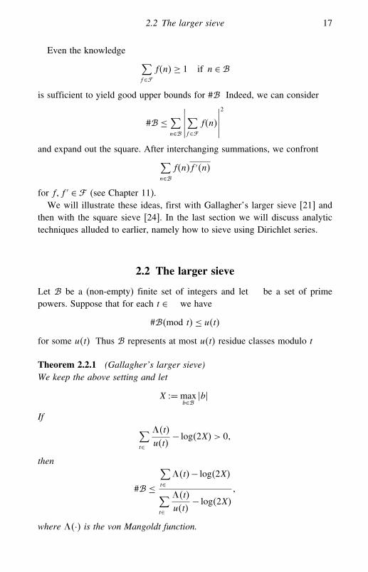
Even the knowledge ∑f∈�f�n�≥ 1 if n ∈

is sufficient to yield good upper bounds for # Indeed, we can consider

#≤ ∑n∈

∣∣∣∣∣∑f∈�f�n�

∣∣∣∣∣2

and expand out the square. After interchanging summations, we confront∑n∈f�n�f ′�n�

for f� f ′ ∈ � (see Chapter 11).We will illustrate these ideas, first with Gallagher’s larger sieve [21] and

then with the square sieve [24]. In the last section we will discuss analytictechniques alluded to earlier, namely how to sieve using Dirichlet series.

2.2 The larger sieve

Let be a (non-empty) finite set of integers and let be a set of primepowers. Suppose that for each t ∈ we have

#�mod t�≤ u�t�for some u�t� Thus represents at most u�t� residue classes modulo t

Theorem 2.2.1 (Gallagher’s larger sieve)We keep the above setting and let

X =maxb∈

�b�If ∑

t∈

��t�

u�t�− log�2X� > 0�

then

#≤

∑t∈��t�− log�2X�

∑t∈

��t�

u�t�− log�2X�

�

where ��·� is the von Mangoldt function.


Proof Let t ∈ and for each residue class r�mod t� define

Z�� t� r� = # �b ∈ b ≡ r�mod t��

Then

#= ∑r�mod t�

Z�� t� r�

By the Cauchy–Schwarz inequality, this is

≤ u�t�1/2( ∑r�mod t�

Z�� t� r�2)1/2

Hence

�#�2

u�t�≤ ∑r�mod t�

∑b�b′∈

b�b′≡r�mod t�

1

≤ #+ ∑b�b′∈b �=b′

∑t�b−b′

1

We multiply this inequality by ��t� and we sum over t ∈ Using∑t�n��t�= logn�

we obtain∑t∈

�#�2

u�t��t�≤ �#�∑

t∈��t�+ �log2X� (�#�2−#

)

By cancelling the # and rearranging, we establish the inequality. �

This sieve should be compared with the large sieve discussed in Chapter 8.The advantage here is that we can sieve out residue classes modulo primepowers, whereas in the large sieve only residue classes modulo primes areconsidered. This explains to some extent the name ‘the larger sieve’.

Following Gallagher, we apply the larger sieve to prove:

Theorem 2.2.2 Let a�b be integers having the property that for any primepower t there exists an integer �t such that

b ≡ a�t �mod t�

Then there exists an integer � such that

b = a�

2.2 The larger sieve 19

Before proceeding with the proof of this theorem, let us review some basicproperties of the cyclotomic polynomial. Recall that for a positive integer d�the d-th cyclotomic polynomial �d�x� is the minimal polynomial over � ofa primitive d-th root of unity. Thus it has degree ��d�, where ��·� is Euler’sfunction. Now let n be an arbitrary positive integer. As the n-th roots of unitycan be partitioned according to their order, we see that we have the formula

xn−1=∏d�n�d�x�

Finally, for an integer a such that �a�n� = 1� let fa�n� be the order of amodulo n By Exercise 6 we have that fa�n�= d if and only if n��d�a�Proof of Theorem 2.2.2 Let a�b be as in the statement of the theorem. Wenote that to prove the result, we may suppose that a�b are positive and a≥ 3(see Exercise 5).

Let

= {n≤ x n= aibj for some i� j

}and

= �t t prime power � fa�t�≤ y� �where y = y�x� is some parameter to be chosen later. By Exercise 6, is afinite set.

We keep the notation of Theorem 2.2.1. If for every prime power t wehave that b is a power of a modulo t� then

u�t�≤ fa�t�Thus Theorem 2.2.1 implies that

#≤

∑t∈��t�− log�2x�

∑t∈

��t�

fa�t�− log�2x�

� (2.3)

provided that the denominator is positive.We have ∑

t∈��t� = ∑

d≤y

∑fa�t�=d

��t�

= ∑d≤y

∑t��d�a�

��t�

= ∑d≤y

log�d�a��


upon using Exercise 6 and the formula∑d�n ��d�= logn Clearly,

�a−1��d� ≤ ��d�a�� ≤ �a+1��d��

so that ∑t∈��t�= ∑

d≤ylog ��d�a��

∑d≤y��d�� y2

We also note that this implies

∑t∈

��t�

fa�t�≥ 1y

∑t∈��t�� y

Now choose

y = 100 log�2x�

From (2.3) we deduce that

#� logx (2.4)

To this end, let us remark that if all the powers of a and b are distinct, thenthe set has cardinality

� �logx�2

(see Exercise 7). This contradicts (2.4), and so we conclude that for somei0� j0 we have

ai0 = bj0 We may even suppose that �i0� j0�= 1� for otherwise we can take �i0� j0�-throots of both sides of the above equality.

Let us write

n=∏p

p�p�n�

for the unique factorization of an integer n into prime powers. We deducethat

i0�p�a�= j0�p�b�for all primes p As �i0� j0�= 1� this means that i0��p�b� and j0��p�a� for allprimes p This implies that a is a j0-th power and b is an i0-th power of someinteger c The hypothesis now implies that for any prime q there exists a �qsuch that

cj0�q ≡ ci0�mod q��

which is equivalent to fc�q��j0�q− i0� if �q� c�= 1

2.3 The square sieve 21

Now take a prime divisor q of �j0t�c� for any t By Exercise 6 we deducethat fc�q�≡ 0�mod j0� Thus j0�i0� and so b is a power of a� as desired. �

2.3 The square sieve

The square sieve is a simple technique originating in [24] meant to estimatethe number of squares in a given set of integers. It relies on the use of a familyof quadratic residue symbols for sifting out the squares. Consequently, it iswell-suited for those sequences that are uniformly distributed in arithmeticprogressions.

Theorem 2.3.1 (The square sieve)Let � be a finite set of nonzero integers and let � be a set of odd primes. Set

S�� = # �� ∈� � is a square �

Then

S��≤ #�#�

+ maxq1 �=q2q1�q2∈�

∣∣∣∣∣∑�∈�

(�

q1q2

)∣∣∣∣∣+E�where

(·

q1q2

)denotes the Jacobi symbol and

E = O(

1#�

∑�∈��+

1�#��2

∑�∈��

2

)�

�� =∑p∈�p��

1

Remark 2.3.2 In practice, the contribution from E is negligible and onewould expect the larger contributions to the estimate to come from the firsttwo terms.

Proof We begin by observing that if � ∈� is a square, then

∑q∈�

(�

q

)= #�−��

Thus

S��≤ ∑�∈�

1�#��2

(∑q∈�

(�

q

)+��

)2

(2.5)


Upon squaring and interchanging the summations, we get that the righthand side of inequality (2.5) is

∑�∈�

1�#��2

( ∑q1�q2∈�

(�

q1

)(�

q2

)+2��

∑q∈�

(�

q

)+��2

)

The first sum is∑q1�q2∈�

1�#��2

∑�∈�

(�

q1

)(�

q2

)≤ #�

#�+ ∑q1�q2∈�q1 �=q2

1�#��2

∑�∈�

(�

q1q2

)

≤ #�#�

+ maxq1�q2∈�q1 �=q2

∣∣∣∣∣∑�∈�

(�

q1q2

)∣∣∣∣∣ The contribution to (2.5) from the latter sums is easily seen to be

E ≤ 2#�

∑�∈��+

1�#��2

∑�∈��

2


Corollary 2.3.3 Let � be a set of nonzero integers and let � be a set ofprimes that are coprime to the elements of � Then

S��= # �� ∈� � is a square �≤ #�#�

+ maxq1�q2∈�q1 �=q2

∣∣∣∣∣∑�∈�

(�

q1q2

)∣∣∣∣∣

Proof The hypothesis of the corollary implies that ��= 0 for any �∈��so that E = 0 in the square sieve. �

We want to apply the square sieve to count the number of integral pointson a hyperelliptic curve

y2 = f�x��where f�x� ∈ ��x� is a polynomial of degree d, of non-zero discriminant,and which is not the perfect square of a polynomial with integer coefficients.A famous theorem of Siegel [67] tells us that the number of integral pointson such a curve is finite. Recently, effective estimates of this number havebeen given by various authors (see [30]). However, these estimates involveknowing the Mordell-Weil rank of the Jacobian of the hyperelliptic curve. Ourapproach is elementary and can be adapted to study how often a polynomialf�x1� � xn� represents a square. As will be seen below, the generalization

2.3 The square sieve 23

will require the deep work of Deligne (see [62]). For more applications, thereader may consult [7].

Given f�x� ∈ ��x� and k ∈ � let us set for k > 2,

Sf �k� =∑

a�mod k�

(f�a�

k

)�

where �·/k� is the Jacobi symbol.

Lemma 2.3.4 Let q1� q2 be distinct primes and let f ∈ ��x� Then

Sf �q1q2�= Sf1�q1�Sf2�q2��where f1�x� = f�q2x�� f2�x� = f�q1x�

Proof The residue classes modulo q1q2 can be written as

q1a2+q2a1�with 0 ≤ a2 ≤ q2−1�0 ≤ a1 ≤ q1−1 (see Exercise 8). Therefore

Sf �q1q2� =q1−1∑a2=0

q2−1∑a1=0

(f�q1a2+q2a1�

q1q2

)

=q1−1∑a2=0

q2−1∑a1=0

(f�q1a2+q2a1�

q1

)(f�q1a2+q2a1�

q2

)

=q1−1∑a2=0

q2−1∑a1=0

(f�q2a1�

q1

)(f�q1a2�

q2

)

The result follows. �

Now let H be a positive real number and let us consider the set

� = �f�n� �n� ≤H� By the square sieve, the number of squares of � is, for any set of primes �not dividing the discriminant of f ,

≤ 2H+1#�

+ maxq1�q2∈�q1 �=q2

∣∣∣∣∣∑�n�≤H

(f�n�

q1q2

)∣∣∣∣∣+E�where

E = O(H logH#�

+ H�logH�2

�#��2

)

and where we have used the elementary estimate ��= O�log��


Let q1� q2 be two distinct primes of � . We have

∑�n�≤H

(f�n�

q1q2

)= ∑a�mod q1q2�

(f�a�

q1q2

) ∑�n�≤H

n≡a�mod q1q2�

1

The inner sum is2Hq1q2

+O�1��

so we obtain ∑�n�≤H

(f�n�

q1q2

)= 2Hq1q2

∑a�mod q1q2�

(f�a�

q1q2

)+O�q1q2�

By the lemma, the sum on the right-hand side is the product Sf1�q1�Sf2�q2�for appropriate polynomials f1� f2We invoke a celebrated result of Weil (see [35, p. 99]), asserting that,

for any g�x� ∈ ��x� with non-zero discriminant and which is not the perfectsquare of a polynomial with integer coefficients, and for any prime p notdividing the discriminant of g,∣∣∣∣∣

∑a�mod p�

(g�a�

p

)∣∣∣∣∣≤ �deg g−1�√p

Using this in the above estimates gives

∑�n�≤H

(f�n�

q1q2

)= O

(H√q1q2

+q1q2)

Let us choose the set � to be given by the primes not dividing the discrim-inant of f and lying in the interval �z�2z� for some z= z�H� > 0� to be alsochosen soon. We get the final estimate

S�� H log zz

+ Hz+ z2+ H�logH��log z�

z+ H�logH�

2�log z�2

z2

Choosing

z =H1/3�logH�2/3

proves:

Theorem 2.3.5 Let f be a polynomial with non-zero discriminant and inte-ger coefficients, which is not the perfect square of a polynomial with integralcoefficients. Let H> 0 Then the number of squares in the set

�f�n� �n� ≤H�

2.4 Sieving using Dirichlet series 25

is O(H2/3�logH�4/3

)� with the implied O-constant depending only on the

degree of f and the coefficients of f .

2.4 Sieving using Dirichlet series

Sometimes, the sequences of numbers that we sift from exhibit a multiplicativestructure and the sieve conditions may also exhibit such a property. In suchcases, analytic methods using Dirichlet series are quite powerful and direct.In some instances, the techniques may even yield asymptotic formulae forthe sieve problem. We illustrate this idea below, in greater detail. Furtherelaboration can be found in [46].

Let � be a set of primes and let � indicate its complement in the set of allprimes. Suppose that we want to count the number of natural numbers n≤ xwhich are not divisible by any of the primes of � If we define the Dirichletseries

F�s�= ∑n≥1

anns= ∏

p∈�

(1− 1

ps

)−1

�

we see that an = 1 if n is not divisible by any p ∈ � and an = 0 otherwise.Thus we seek to study ∑

n≤xan

By Perron’s formula (see [45, pp. 54–7]), this can be written as∑n≤xan =

12�i

∫ 2+i

2−iF�s�

xs

sds

Here is a variant of the classical Tauberian theorem that is useful in sucha context.

Theorem 2.4.1 (Tauberian theorem)

Let F�s�=∑n≥1

anns

be a Dirichlet series with non-negative coefficients converg-

ing for Re�s� > 1. Suppose that F�s� extends analytically at all points onRe�s�= 1 apart from s = 1, and that at s = 1 we can write

F�s�= H�s�

�s−1�1−�

for some � ∈ � and some H�s� holomorphic in the region Re�s� ≥ 1 andnonzero there. Then ∑

n≤xan ∼

cx

�logx��


with

c = H�1��1−��

where � is the usual Gamma function.

This theorem was proven in 1938 by Raikov [54]. We do not prove ithere, but only indicate that standard techniques of analytic number theory, asexplained in [45, Chapter 4], can be used to derive the result. The reader mayalso find treatments in English in [75] and [68].

As an illustration of the principle, we consider the problem of counting thenumber of natural numbers n≤ x that can be written as the sum of two squares.It is well-known (see [32, p. 279]) that n can be written as a sum of twosquares if and only if for every prime p≡ 3�mod 4� dividing n, the power ofp appearing in the unique factorization of n is even. Thus, if an = 1 whenevern can be written as a sum of two squares and is zero otherwise, we see that

F�s� = ∑n≥1

anns

=(1− 1

2s

)−1 ∏p≡1�mod 4�

(1− 1

ps

)−1 ∏p≡3�mod 4�

(1− 1

p2s

)−1

Now we need to invoke some basic properties of the Riemann zeta func-tion ��s� and the Dirichlet L-function L�s��4� associated with the quadraticcharacter �4, defined by

��s� = ∑n≥1

1ns� L�s��4� =

∑n≥1

�4�n�

ns

for s ∈ � with Re�s� > 1 Here, �4�n� is 0 for n even and �−1��n−1�/2 for nodd. We refer the reader to [45] for the properties of these functions. Usingthe Euler products of ��s� and L�s��4� we write

F�s�= ��s�L�s��4��1/2H1�s��

where H1�s� is analytic and non-vanishing for Re�s� > 1/2 As L�s��4�extends to an entire function and is non-vanishing for Re�s�≥ 1� we have

F�s�= ��s�1/2H2�s�

for some H2�s� holomorphic and nonzero in Re�s� ≥ 1 Thus, using the factthat the Riemann zeta function has a simple pole at s= 1 and that it is analyticand non-vanishing for Re�s�= 1� s �= 1 (see [45]), we deduce that

F�s�= H�s�

�s−1�1/2�

with H�s� holomorphic and non-vanishing in the region Re�s�≥ 1.By the Tauberian theorem cited above we obtain:

2.5 Exercises 27

Theorem 2.4.2 The number of n≤ x that can be written as the sum of twosquares is

∼ cx√logx

for some c > 0� as x→

By the same technique using classical Dirichlet series, one can also deducethe following remarkable result. Fix an integer k ≥ 3. The number of n ≤ xnot divisible by any prime p≡ 1�mod k� is

∼ c1x

�logx�1/��k�

for some c1 > 0, where ��k� is the Euler function. Thus a consequence ofthis result is that ‘almost all’ numbers have a prime divisor p≡ 1�mod k�

Further applications of the technique can be found in [46].

2.5 Exercises

1. (The Cauchy–Schwarz inequality)

Let �ai�1≤i≤n� �bi�1≤i≤n be complex numbers. Show that

∣∣∣∣∣∑

1≤i≤naibi

∣∣∣∣∣2

≤( ∑

1≤i≤n�ai�2

)( ∑1≤i≤n

�bi�2)

2. Let k < n be positive integers. Let X be a k-element set and Y =�y1� � yn� an n-element set. Let S be the set of all maps from X toY , and �i be the set of maps whose image does not contain yi Thenthe set

S\∪1≤i≤n�i

consists of maps that are surjective. Using the inclusion–exclusionprinciple, deduce that

∑0≤i≤n

�−1�i(n

i

)�n− i�k = 0

whenever k < n


3. Prove that ∑0≤i≤n

�−1�i(n

i

)�n− i�n = n!

4. Let � = �1�2� � n� Denote by Dn the number of one-to-one mapsf �−→� without any fixed point. Show that

limn→

Dnn! = 1

e�

where e denotes Euler’s e.[A map f without any fixed point is called a derangement].

5. Let a�b be integers. We say that a and b are related if, for every primepower t,

b ≡ a�t �mod t�

for some positive integer �t Show that if a and b are related, so are a2

and b2 Also, show that if �a� ≤ 2 and �b� ≤ 2 with a�b related, then�a� = �b�

6. If t is a prime power coprime to k, show that t��k�a� if and only ifa�mod t� has order k

7. If a and b are natural numbers ≥ 2 with{ai i ≥ 1

}∩{bj j ≥ 1

}= ∅�show that the number of aibj ≤ x is

� �logx�28. Let t1� t2 be coprime positive integers and let t = t1t2 Show that all

the residue classes modulo t can be represented as

t1a2+ t2a1for some 0 ≤ a2 ≤ t2−1�0 ≤ a1 ≤ t1−1 Also, show that the coprimeresidue classes modulo t can be represented as above with �a2� t2� =�a1� t1�= 1

9. For any f�x� ∈ ��x� and any natural number k > 2� define

Sf �k� =∑

a�mod k�

(f�a�

k

)�

where (·/k) is the Jacobi symbol. If k = ∏iq�ii is the unique prime

factorization of k, then there exist polynomials fi such that

Sf �k�=∏i

Sfi(q�ii

)

2.5 Exercises 29

10. A number n is called squareful if for every prime p�n we have p2�nShow that the number of squareful natural numbers ≤ x is

∼c1√x

for some c1 > 0, as x→11. Let k be a natural number ≥ 3 Show that the number of n≤ x that are

not divisible by any prime p≡ 1�mod k� is

∼ c2x

�logx�1/��k�

for some c2 > 0, as x→12. Show that, for any positive integer n�

∑d�n��d�= logn

13. Show that

�a−1��d� ≤ ��d�a�� ≤ �a+1��d�

and ∑d≤x��d�� x2

14. Let ��x� y� denote the number of n ≤ x with the property that if aprime p�n, then p < y. Show that if x1/2 < z≤ x, then

��x� z�=(1− log

(logxlog z

))x+O

(x

log z

)

[A number all of whose prime factors are < y is called a y-smoothnumber.]

15. Prove that if y < z, then

��x� y�=��x� z�− ∑y≤p<z

∑r=1

��x/pr�p�

Deduce that

��x� y�=��x� z�− ∑y≤p<z

� �x/p�p�+O�x/y�

[This is often referred to as Buchstab’s identity.]16. For x1/3 ≤ y ≤ x1/2, show that

��x� y�∼ x��u��where u = logx/ logy and

��u� = 1− logu+∫ u

2log�v−1�

dvv

[Hint: use Buchstab’s identity and partial summation.]


17. Define ��u� recursively by ��u� = 1 for 0 ≤ u ≤ 1 and, for positiveintegers k, by

��u�= ��k�−∫ u

k��v−1�

dvv

for k < u ≤ k+ 1. Using Buchstab’s identity, deduce inductively thatfor any � > 0 and x� < y ≤ x, we have the asymptotic formula

��x� y�∼ x��u�with u = logx/ logy. [��u� is called Dickman’s function and wasdiscovered by K. Dickman in 1930. For further details on this function,as well as more results concerning ��x� y�, we refer the reader to[68, p. 367].]

18. Suppose that A is a subset of natural numbers contained in the interval�1� x� whose image modulo every prime p has size O�p1/2�. Show that#A= O�logx�.

19. Let A be a set of natural numbers and let P be a set of prime numbers.Let �P� denote the semigroup generated by elements of P. Then anyinteger n can be written uniquely as n= nPm� where nP ∈ �P� and mis coprime to p for all p ∈ P. Show that

∑d�nd∈�P�

��d�

equals 1 if nP = 1 and zero otherwise. If �P�n� is defined to be logpwhenever n= pa for some prime p ∈ P and zero otherwise, then showthat

�P�n�=− ∑d�nd∈�P�

��d� logd

whenever nP > 1.

20. With notation as in the previous exercise, let A be a set of naturalnumbers ≤ x and let S�A�P� denote the set of elements n of A withnP = 1. Now suppose:

(i) for d ∈ �P�, the set Ad consisting of elements of A divisible by dsatisfies

#Ad = �x

d+R�x�d�

2.5 Exercises 31

for some � and some R�x�d� with∑d≤xd∈�P�

�R�x�d�� log xd= O�x��

(ii) if n ∈A with nP > 1, then nP has at least two prime factors countedwith multiplicity;

(iii) there is a set B such that S�A�P� = S�B�P� and satisfying thecondition that for p ∈ P and m ∈ B, we have pm ∈ B;

(iv) there are numbers a and b with a > 0 so that

∑m≤xm∈B

1m

= a logx+b+O(1x

)

Under these conditions, show that for some positive constant c,

#S�A�P�∼ cx

�logx�1−a/b

as x tends to infinity.21. Apply the previous exercise to the set A consisting of natural numbers≡

1�mod 4� and P the set of primes ≡ 3�mod 4�. Thus, deduce Theorem2.4.2. [Hint: take B to be the set of odd natural numbers.]The last two exercises have been adapted from [52].

22. Let f�x� be a polynomial with integer coefficients having the propertythat for every integer n, f�n� is a perfect square. Show that f�x� is thesquare of a polynomial with integer coefficients. Generalize this resultto polynomials of several variables. [Hint: this can be deduced withoutusing the results obtained in this chapter on the square sieve, as follows.We may suppose without loss of generality that f�x� is a product ofdistinct irreducible polynomials. Take a prime p that is coprime to thediscriminant of f such that p�f�n� for some n. Consider f�n+p� andf�n� and deduce that one of them is not divisible by p2. The generalcase can be formally treated using resultants and made to reduce to thesingle variable case.]

3The normal order method

The normal order method has its origins in a 1916 paper of G. H. Hardy(1877–1947) and S. Ramanujan (1887–1920). A simpler and more transparenttreatment of their work was given later in 1934 by Paul Turán (1910–76).Turán’s method was substantially amplified by Paul Erdös (1913–96) andMark Kac (1914–84). They used it to create an entire subject that has cometo be known as probabilistic number theory.

The method of Turán will be discussed in greater detail in the next chapter,which will form the basis for an elementary sieve method. In this chapter wewill focus on how Turán’s method can be used to study the distribution ofthe number of prime factors of various sequences of numbers.

3.1 A theorem of Hardy and Ramanujan

We recall that ��n� denotes the number of distinct prime divisors of n. In1916, Hardy and Ramanujan (see [28, p. 356]) proved that almost all numbersn are composed of log logn prime factors. To be precise, they showed thatthe number of n≤ x not satisfying the inequality

�1−�� log logn < ��n� < �1+�� log logn

is o�x� for any given � > 0. Their proof involved an elaborate inductionargument and was rather long and complicated. In 1934, Turán gave a simplerproof of their result. We begin by presenting Turán’s proof. After that, wediscuss the application of the technique to a wider context. In the next chapter,we will isolate a combinatorial sieve method from it, which we call the Turánsieve.

32

3.1 A theorem of Hardy and Ramanujan 33

Theorem 3.1.1 We have∑n≤x��n�= x log logx+O�x�

and ∑n≤x�2�n�= x�log logx�2+O�x log logx�

Proof Let us observe that, by Theorem 1.4.4,

∑n≤x��n� = ∑

p≤x

[x

p

]

= x∑p≤x

1p+O�x�

= x log logx+O�x�Also, ∑

n≤x�2�n� = ∑

n≤x

∑p�n

∑q�n

1

= ∑p�q≤x

∑n≤xp�n �q�n

1

= ∑p�q≤xp �=q

[x

pq

]+∑p≤x

[x

p

]

= ∑pq≤x

[x

pq

]+O�x log logx�

= x ∑pq≤x

1pq

+O�x log logx�

Now, ( ∑p≤√

x

1p

)2

≤ ∑pq≤x

1pq

≤(∑p≤x

1p

)2

Since

∑p≤√

x

1p= log log

√x+O�1�= log logx+O�1��

34 The normal order method

we find that ∑n≤x�2�n�= x�log logx�2+O�x log logx�


Now consider the variance∑n≤x��n�− log logx�2 = ∑

n≤x�2�n�−2�log logx�

∑n≤x��n�+ �log logx�2

∑n≤x

1�

which is easily seen to be O�x log logx� by what we have proven above. Thisshows:

Theorem 3.1.2 (Turán)∑n≤x��n�− log logx�2 = O�x log logx�

Corollary 3.1.3 Let � > 0. The number of n ≤ x that do not satisfy theinequality

��n�− log logx�< �log logx�12+�

is o�x�.

Proof Indeed, if n ≤ x does not satisfy the inequality, then a summandcoming from n satisfies

��n�− log logx� ≥ �log logx�1/2+�

The theorem implies that the number of such n≤ x is

O(x�log logx�−2�

)= o�x��

Hardy and Ramanujan prove, in fact, a stronger theorem, getting a moreprecise estimate for the exceptional set. As already mentioned, the proof wehave given is due to Turán (see, for example, [28, pp. 354–8]).

Related to the above results there is a celebrated theorem of Erdös and Kac(see [11, 12]), which states that, if for �≤ �,

S�x�� = #

{n≤ x �≤ ��n�− log logn√

log logn≤ �

}�

3.2 The normal number of prime divisors of a polynomial 35

then

limx→

S�x��

x= 1√

2�

∫ �

�e−t

2/2dt

The integral is the familiar probability integral associated with the normaldistribution. Thus, the theorem of Erdös–Kac says that the function

��n�− log logn√log logn

is ‘normally distributed’ in a suitable probabilistic sense. We refer the readerto [11, 12] for further details.

We say that a function f�n� has normal order F�n� if, for every � > 0,the inequality

�1−��F�n� < f�n� < �1+��F�n�is satisfied for almost all values of n. That is, the number of n ≤ x that donot satisfy the inequality is o�x�.

It is now not difficult to establish that ��n� has normal order log logn (seeExercise 1).

3.2 The normal number of prime divisors of a polynomial

Let f�x� be an irreducible polynomial with integer coefficients. We wouldlike to consider the problem of determining the normal order of ��f�n��. Forthis purpose, we proceed as in the previous section. The details follow.

First, let us observe that if �y�n� denotes the number of primes dividing nthat are ≤ y and if y = x� for some 0< � < 1/2, then for n≤ x we have

��n�= �y�n�+ ��n�−�y�n��= �y�n�+O�1��since the number of prime divisors of n greater than y is O�1�. We cantherefore write ∑

n≤x��f�n��= ∑

n≤x�y�f�n��+O�x� (3.1)

Let us denote by �f �p� the number of solutions modulo p of the congruencef�x�≡ 0�mod p�. Then ∑

n≤x�y�f�n��=

∑n≤x

∑p�f�n�p≤y

1� (3.2)


so that, upon interchanging summation, we must count, for fixed p, thenumber of integers n≤ x that belong to �f �p� residue classes modulo p. Weobtain ∑

n≤x��f�n��= ∑

p≤y

(x�f �p�

p+O��f �p��

)+O�x�� (3.3)

and since �f �p� ≤ degf , we see that the error term arising from the abovesummation is O�y�.

At this point we need to invoke some algebraic number theory. Let K =�� where � is a solution of f�x� = 0. The ring of integers �K of K is aDedekind domain. It is a classical theorem of Dedekind (see Theorem 5.5.1of [17]) that for all but finitely many primes p, �f �p� is the number of primeideals � of �K such that the norm NK/��= p. If �K�x� denotes the numberof prime ideals whose norm is ≤ x, then the analogue of the prime numbertheorem for number fields asserts that

�K�x�∼x

logx

as x→. In fact, for some constant c > 0,

�K�x�= lix+O�xe−c√

logx��

where

lix =∫ x

2

dtlog t

is the famous logarithmic integral (let us note that, upon integration by parts,lix = x/logx+O (

x/log2 x)). Since the norm of any prime ideal is a prime

power and since the number of prime ideals whose norm is not a prime cannotexceed O�

√x logx�, we deduce:

Theorem 3.2.1 (The prime ideal theorem)∑p≤x�f �p�= lix+O�xe−c

√logx�

for some c > 0.

By partial summation we deduce further:

Corollary 3.2.2 ∑p≤x

�f �p�

p= log logx+O�1�

3.2 The normal number of prime divisors of a polynomial 37

We can now complete our analysis of the normal order of ��f�n��. By ourearlier discussion ((3.1), (3.2), (3.3)) and the corollary above,∑

n≤x��f�n��= x log logx+O�x�

Also,

∑n≤x�2�f�n�� = ∑

n≤x�2y �f�n��+O

(∑n≤x�y�f�n��

)

= ∑n≤x�2y �f�n��+O�x log logx�

We find by the Chinese remainder theorem that

∑n≤x�2y �f�n��=

∑p�q≤yp �=q

(x�f �p��f �q�

pq+O�1�

)+O�x log logx��

where the latter error term arises from terms where p= q. Since∑p

�f �p�2

p2= O�1��

we have

∑p�q≤yp �=q

�f �p��f �q�

pq=

(∑p≤y

�f �p�

p

)2

+O�1�

Thus ∑n≤x�2y �f�n��= x�log logx�2+O�y2�+O�x log logx�

Now we recall that y = x� with 0 < � < 1/2, and so the O�y2� error term isdominated by O�x log logx�. This proves:

Theorem 3.2.3 ∑n≤x��f�n��− log logx�2 = O�x log logx�

It is now an elementary exercise to deduce the normal order of ��f�n�� aslog logn.

Theorem 3.2.3 gives an estimate of

� x

log logx


for the number of n ≤ x such that f�n� is prime. A classical conjecture ofBuniakowski formulated in 1854 predicts that any irreducible polynomialf�x� ∈ ��x�, such that f��+� has no common divisor larger than 1, repre-sents primes infinitely often. The only known case of this conjecture is thecelebrated theorem of Dirichlet about the distribution of primes in an arith-metic progression, which settles it in the linear case. We will see later (usingmethods of Chapters 6 and 10) that sieve techniques can be applied to shedsome light on this conjecture. In some cases, the methods come very close tosettling it.

One can also establish the analogue of the Erdös–Kac theorem for ��f�n��.This has been done in [49].

If f is not irreducible, but has r irreducible factors, then the prime idealtheorem implies ∑

p≤x�f �p�∼

rx

logx

as x→. It will be of interest to make this effective and investigate whethersuch a result can be used to give an efficient ‘primality test’ or ‘irreducibilitytest’ for an arbitrary f ∈ ��x�.It would also be of interest to generalize these investigations to study poly-

nomials of several variables. This leads to the study of polynomial congru-ences modulo p in several variables, about which much is known thanks tothe spectacular development of modern algebraic geometry (see, for example,the excellent monograph of Ireland and Rosen [32] for an introduction).

3.3 Prime estimates

We can investigate in a similar way ��p−1� as p varies over the primes. Moreprecisely, let k be a natural number and define for �a� k�= 1 the quantity

��x�k�a� = # �p ≤ x p≡ a�mod k��

Then it is easily seen that∑p≤x��p−1�=∑

≤x��x� �1��

where we recall that denotes a rational prime. As before, it is convenient toobserve that, by an application of Chebycheff’s theorem,

∑p≤x��p−1�= ∑

p≤x�y�p−1�+O

(x

logx

)�

3.3 Prime estimates 39

so that we obtain sums of the form∑ ≤y��x� �1�

to investigate with y = x� for some � > 0.A classical theorem of Bombieri and Vinogradov states that, for any A> 0,

there is a B = B�A� > 0 so that

∑k≤x1/2 log−B x

maxy≤x max

�a�k�=1

∣∣∣��y�k�a�− li y��k�

∣∣∣� x

logA x

This theorem will be proven in Chapter 9. In fact, much of the developmentof the large sieve method (to be discussed in Chapter 8) culminated in itsproof. We invoke this theorem to deduce

∑ ≤y��x� �1�=∑

≤y

lix −1

+O(

x

logA x

)�

provided � < 1/2. Since

∑ ≤y

1 −1

=∑ ≤y

1 +O�1��

we conclude that∑p≤x��p−1�= ��x� log logx+O

(x

logx

)

In a similar way we deduce that (see Exercise 9)∑p≤x�2�p−1�= ��x��log logx�2+O��x� log logx�

This establishes the following theorem of Erdös:

Theorem 3.3.1 (Erdös’ theorem)

∑p≤x��p−1�− log logp�2 = O

(x log logx

logx

)

Again, it is possible to establish the analogue of the Erdös–Kac theorem for��p−1�. In a recent paper [38], it is shown how one may prove this theoremwithout using the Bombieri–Vinogradov theorem but rather a ‘weighted’version of the Turan sieve discussed in the next chapter.

A similar investigation can be made for the study of ��p−a� for any integera The case a=−2 is related to the well-known twin prime conjecture. Tobe precise, a prime p is called a twin prime if p+ 2 is also a prime; it is


conjectured that there are infinitely many such primes. An interesting corollaryof the analogues of Theorem 3.3.1 for ��p+ 2� will be that the number ofprimes p ≤ x such that p+2 is also a prime is

O

(��x�

log logx

) (3.4)

However, it is to be noted that we have proven (3.4) by assuming theBombieri–Vinogradov theorem, which in turn is derived from the large sieve.The latter method is capable of yielding superior estimates for the number oftwin primes, as will be discussed in Chapter 10.

3.4 Application of the method to other sequences

Having in mind the main steps for the proofs of Theorems 3.1.2, 3.2.3 and3.3.1, we deduce that the normal order method can be formalized as follows.

Let � = �an� be a finite sequence of natural numbers. Let �1 =� andfor each squarefree d, define

�d = �an an ≡ 0�mod d��

For each squarefree d, we will write

#�d =��d�

dX+Rd�

or even

#�d = �dX+Rd�where we think of X as an approximation to the cardinality of � and of R1

as the error in the approximation. The function �d =��d�/d is to be thoughtof as the ‘proportion’ of the elements of � belonging to �d. In particular,for primes p and q we write

#�p =��p�

pX+Rp

and

#�pq =��pq�

pqX+Rpq

Now suppose that

an = O�nC�

3.4 Application of the method to other sequences 41

for some positive constant C. As before, we can show that∑n≤x��an�=

∑n≤x�y�an�+O�x�

for some y = x� and � > 0. Then we find

∑n≤x��an�=

∑p≤y

��p�

pX+∑

p≤yRp+O�x�

and we see that, in order to proceed further, we would need the asymptoticbehaviour of ∑

p≤y

��p�

p

and an estimate for the sum of the error terms∑p≤yRp

Similarly, the study of ∑n≤x�2�an�

would lead to finding an estimate for the sum∑p�q≤y

Rpq

We will develop a general sieve out of this method in the next chapter.In the example of Section 3.1, an = n, X = x and ��p�= 1. In the example

of Section 3.2, an = f�n� with f an irreducible polynomial ∈��x�, X = x and��p�= �f �p�. In the case an = pn−1 where pn denotes the n-th prime andpn ≤ x, we have X = ��x� and ��p�= p/�p−1�.There are many other interesting applications of this method. For example,

let g be a nonzeromultiplicative function (that is, g�mn�= g�m�g�n� for anycoprime integers m�n), taking rational integer values and such that g�n� �= 0for every natural number n (this assumption can be relaxed somewhat (see[48])). Define

�g�x�d� = #�p ≤ x g�p�≡ 0�mod d��

Let us assume:�H0� for some � > 0, �g�n�� ≤ n� for all n;�H1� for some � > 0�∑

d≤x��g�x�d�−��d��x��

x

logx�


�H2� for prime powers p��q� (p �= q�,��p��= p−�+O�p−�−1�

and

��p�q��= �p−�+O�p−�−1��q−�+O�q−�−1��

where the implied constants are absolute.The following is proven in [49]:

Theorem 3.4.1 Denote by

N�x�� = #{n≤ x ��g�n��−

12 �log logn�2

�log logn�3/2≤ �√

3

}�

where g satisfies �H0�� H1�� H2� above. Then

limx→

N�x��

x= 1√

2�

∫ �

−e−t

2/2dt

Under the same hypotheses, one can also show that∑p≤x��g�p��− log logp�2 = O��x� log logx��

and, more generally, a theorem of Erdös–Kac type for ��g�p��. To be precise,if we let

S�x�� = #{p ≤ x ��g�p��− log logp√

log logp≤ �

}�

then

limx→

S�x��

��x�= 1√

2�

∫ �

−e−t

2/2dt

These results have been established in [48, 49].Theorem 3.4.1 can, for instance, be applied to ��n��. In [16], Erdös

and Pomerance determined the normal order of ��n�� using the Bombieri–Vinogradov theorem. In [50], Murty and Saidak show that the same result canbe established without this theorem and by using only the elementary sieveof Eratosthenes (to be discussed in Chapter 5).

To cite a ‘modular’ example, consider the Ramanujan function ��n�defined as the coefficient of xn in the infinite product

x∏m=1

�1−xm�24

3.5 Exercises 43

By invoking the theory of -adic representations (see [63, 64]), one canprove certain properties about the number of prime divisors of ��n�. In 1916,Ramanujan conjectured that ��n� is a multiplicative function. This was provena year later by Mordell (see [61]). One can try to apply Theorem 3.4.1 todetermine the normal number of prime factors of ��n� whenever it is not zero.Such an investigation is caried out in [48, 49]. Hypothesis �H0� is satisfied andhypotheses �H1� and �H2� are satisfied, as well, if we assume the generalizedRiemann hypothesis for certain Artin L-functions. The method does lead tothe interesting conclusion that

��p�� ≥ exp��logp�1−��

for almost all primes p (that is, apart from o �x/logx� primes p ≤ x) andfor any 0 < � < 1. This is related to a classical conjecture of Lehmer (stillunresolved) that ��p� �= 0.Finally, let us mention that the normal order method was recently applied

by Ram Murty and F. Saidak to settle a conjecture of Erdös and Pomeranceconcerning the function fa�p�� which is defined to be the number of primefactors of the order of a modulo p in ��/p��∗, albeit conditionally assumingthe generalized Riemann hypothesis. Precise details can be found in [50].

3.5 Exercises

1. Prove that ∑n≤x��n�− log logn�2 = O�x log logx�

2. Let �y�n� denote the number of prime divisors of n that are less thanor equal to y. Show that

∑n≤x

(�y�n�− log logy

)2 = O �x log logy�

3. Prove that

∑n≤x��n�− log logx�2 = x log logx+O�x�

4. Let �n� denote the number of prime powers that divide n. Showthat �n� has normal order log logn.


5. Fix k ∈ � and let �a� k�= 1. Denote by ��n�k�a� the number of primedivisors of n that are ≡ a�mod k�. Show that ��n�k�a� has normalorder

1��k�

log logn

6. Let g be a non-negative bounded function defined on the primes anddefine

g�n� =∑p�ng�p��

A�n� = ∑p≤n

g�p�

p

Prove that ∑n≤x�g�n�−A�x��2 = O�x log logx�

7. Using Theorem 3.2.1, prove that there is a positive constant c such that

∑p≤x

�f �p�

p= log logx+ c+O

(1

logx

)

8. If f�x� ∈��x� is not irreducible, but has r distinct irreducible factors in��x� (hence in ��x�), deduce that ��f�n�� has normal order r log logn.

9. Using the Bombieri–Vinogradov theorem, prove that∑p≤x�2�p−1�= ��x��log logx�2+O��x� log logx�

10. Let Px denote the greatest prime factor of∏n≤x

(n2+1

)

Show that Px > cx logx for some positive constant c.

11. Show that, as x→,∑a2+b2≤x

��a2+b2�= ��x��log logx�+O�x��

where the summation is over all integers a�b satisfying the inequalitya2+b2 ≤ x.

3.5 Exercises 45

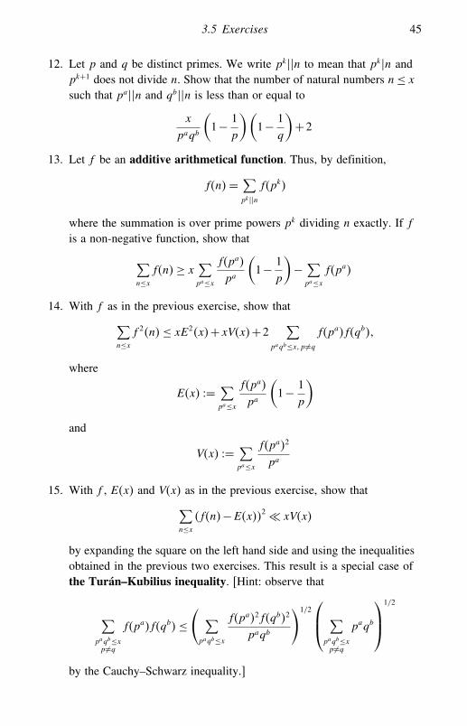
12. Let p and q be distinct primes. We write pk��n to mean that pk�n andpk+1 does not divide n. Show that the number of natural numbers n≤ xsuch that pa��n and qb��n is less than or equal to

x

paqb

(1− 1

p

)(1− 1

q

)+2

13. Let f be an additive arithmetical function. Thus, by definition,

f�n�= ∑pk��nf�pk�

where the summation is over prime powers pk dividing n exactly. If fis a non-negative function, show that

∑n≤xf�n�≥ x ∑

pa≤x

f�pa�

pa

(1− 1

p

)− ∑pa≤x

f�pa�

14. With f as in the previous exercise, show that∑n≤xf 2�n�≤ xE2�x�+xV�x�+2

∑paqb≤x�p �=q

f�pa�f�qb��

where

E�x� = ∑pa≤x

f�pa�

pa

(1− 1

p

)

and

V�x� = ∑pa≤x

f�pa�2

pa

15. With f , E�x� and V�x� as in the previous exercise, show that∑n≤x�f�n�−E�x��2 � xV�x�

by expanding the square on the left hand side and using the inequalitiesobtained in the previous two exercises. This result is a special case ofthe Turán–Kubilius inequality. [Hint: observe that

∑paqb≤xp �=q

f�pa�f�qb�≤( ∑paqb≤x

f�pa�2f�qb�2

paqb

)1/2⎛⎜⎝ ∑paqb≤xp �=q

paqb

⎞⎟⎠

1/2

by the Cauchy–Schwarz inequality.]


16. If f , E�x� and V�x� are as in the previous exercises and V�x� tends toinfinity as x tends to infinity, show that, for any � > 0, the number ofn≤ x with

�f�n�−E�x�� ≥ V�x�1/2+�

is o�x�.17. Extend the result of Exercise 15 to arbitrary real valued additive func-

tions f , as follows. Define additive functions g1�n� and g2�n� by settingg1�p

k� = f�pk� if f�pk� ≥ 0 and zero otherwise, g2�pk� =−f�pk� if

f�pk� < 0 and zero otherwise. Then f�n�= g1�n�−g2�n�. If

Ej�x� =∑pk≤x

gj�pk�

pk

(1− 1

p

)�

then show that

�f�n�−E�x��2 ≤ 22∑j=1

�gj�n�−Ej�x��2

by the Cauchy–Schwarz inequality. Deduce that∑n≤x

�f�n�−E�x��2 � xV�x�

18. Extend the result of the previous exercise to complex valued additivefunctions by considering the real-valued additive functions g1�n� =Re�f�n�� and g2�n� = Im�f�n��. This establishes the Turán–Kubiliusinequality for all complex-valued additive functions.

19. Show that the implied constant in the Turán–Kubilius inequality can betaken to be 32.

20. Show that the factor 32x implied by the previous exercise for theTurán–Kubilius inequality can be replaced by

!�x� = 2x+⎛⎜⎝ ∑paqb≤xp �=q

paqb

⎞⎟⎠

1/2

+4

(∑pa≤x

1pa

∑qb≤xqb

)1/2

Deduce that

lim supx→

!�x�

x≤ 2

4The Turán sieve

In 1934, Paul Turán (1910–76) gave an extremely simple proof of the classicaltheorem of Hardy and Ramanujan about the normal number of prime factorsof a given natural number. Inherent in his work is a basic sieve method, whichwas called Turán’s sieve by the authors of [37], where it was first developed.In this chapter, we will illustrate how this sieve can be used to treat otherquestions that had previously been studied using more complicated sievemethods. For example, the Turán sieve is more elementary than the sieve ofEratosthenes and in some cases gives comparable results.

4.1 The basic inequality

Let � be an arbitrary finite set and let � be a set of prime numbers. Foreach prime p ∈ � we assume given a set �p ⊆�. Let �1 =� and for anysquarefree integer d composed of primes of �� let

�d = ∩p�d�p

Fix a positive real number z and set

P�z� = ∏p∈�p<z

p

We will be interested in estimating

S�� z� = #(�\∪p�P�z��p

)

Following the method illustrated in Section 3.4, we write for each primep ∈ � ,

#�p = �pX+Rp (4.1)

47

48 The Turán sieve

and for distinct primes p�q ∈ ��

#�pq = �p�qX+Rp�q� (4.2)

where

X = #��

0 ≤ �p < 1

For notational convenience, we interpret Rp�p as Rp. Heuristically, we usuallythink of �p as the proportion of elements of� lying in�p, and ofRp as the errorterm in this estimation. The same interpretation can be given to �p�q andRp�q.

Theorem 4.1.1 (The Turán sieve)

We keep the above setting. Let

U�z� = ∑p�P�z�

�p

Then

S�� z�≤ X

U�z�+ 2U�z�

∑p�P�z�

�Rp�+1

U�z�2

∑p�q�P�z�

�Rp�q�

Proof For each element a ∈�, let N�a� be the number of primes p�P�z�such that a ∈�p. Then

S�� z�= #�a ∈� N�a�= 0�≤ 1U�z�2

∑a∈��N�a�−U�z��2

Thus the goal is to derive an upper bound for

∑a∈��N�a�−U�z��2 �

an expression that is reminiscent of the normal order method. Squaring outthe summand and expanding, we must consider

∑a∈�N�a�2−2U�z�

∑a∈�N�a�+XU�z�2

4.2 Counting irreducible polynomials in �p�x� 49

For the first sum we have

∑a∈�N�a�2 = ∑

a∈�

⎛⎜⎜⎝ ∑p�P�z�a∈�p

1

⎞⎟⎟⎠

2

= ∑p�q�P�z�

#�p∩�q

= ∑p�q�P�z�p �=q

#�pq+∑p�P�z�

#�p

= X ∑p�q�P�z�p �=q

�p�q+X∑p�P�z�

�p+∑

p�q�P�z�Rp�q

= X( ∑p�P�z�

�p

)2

−X ∑p�P�z�

�2p+X∑p�P�z�

�p+∑

p�q�P�z�Rp�q�

and, similarly, ∑a∈�N�a�= X ∑

p�P�z��p+

∑p�P�z�

Rp

Here we have used assumptions (4.1) and (4.2). Therefore∑a∈��N�a�−U�z��2 = X ∑

p�P�z��p�1−�p�+

∑p�q�P�z�

Rp�q−2U�z�∑p�P�z�

Rp

Since �1− �p� ≤ 1, we immediately deduce the upper bound stated in thetheorem. �

Remark 4.1.2 In order to use the above theorem, the essential point is tohave upper bounds for Rp�q and Rp� as well as a lower bound for U�z�.

4.2 Counting irreducible polynomials in �p�x�

Let �p denote the finite field of p elements. Fix a natural number n > 1 andlet Nn be the number of monic irreducible polynomials in �p�x� of degree n.There are several ways of obtaining an exact formula for Nn. The simplest isvia a technique of zeta functions, as follows.

Consider the power series ∑f

T deg f �

50 The Turán sieve

where the summation is over all monic polynomials f ∈ �p�x�. Since the totalnumber of monic polynomials f ∈ �p�x� of degree n is pn, the power seriesis easily seen to be

∑n=0

pnTn = 11−pT

On the other hand, �p�x� is a Euclidean domain and so it has unique factor-ization. Thus we can write an ‘Euler product’ expression for the power seriesabove as ∏

v

�1−T deg v�−1 =∏n=1

�1−Tn�−Nn�

where v runs over monic irreducible polynomials of �p�x�. We thereforeobtain

�1−pT�−1 =∏d=1

�1−Td�−Nd (4.3)

By using that

− log�1−pT�=∑n=1

pnTn

n

and taking logarithms in (4.3), we get∑n=1

pnTn

n= − log�1−pT�=−

∑d=1

Nd log�1−Td�

=∑d=1

∑e=1

dNdTde

de=

∑n=1

Tn

n

(∑de=n

dNd

)

This proves:

Theorem 4.2.1 Let Nd denote the number of monic irreducible polynomialsof �p�x� of degree d. Then ∑

d�ndNd = pn

Observe that an immediate consequence is

Nn ≤pn

n�

which can be viewed as the function field analogue of Chebycheff’s upperbound (1.1) for ��x�. In fact, it is easy to deduce that (see Exercise 1)

Nn ∼pn

n�

4.3 Counting irreducible polynomials in ��x� 51

or, more precisely,

Nn =pn

n+O�pn/2d�n��

where d�n� denotes the number of divisors of n. One can view this as theanalogue of the prime number theorem (1.2) for �p�x�.It is possible to invert the above expression for Nn and solve for it via the

Mobius inversion formula. This will give us an explicit formula for Nn. Moreprecisely, by applying Theorem 1.2.2 we deduce from Theorem 4.2.1:

Theorem 4.2.2 Let Nn denote the number of monic irreducible polynomialsof �p�x� of degree n. Then

Nn =1n

∑d�n��d�pn/d

4.3 Counting irreducible polynomials in ��x�

Fix natural numbers H and n > 1We will apply the Turán sieve to count thenumber of irreducible polynomials

xn+an−1xn−1+· · ·+a1x+a0

with 0 ≤ ai ≤H , ai ∈ �. We will prove that this number is

Hn+O�Hn−1/3 log2/3H�

Thus, a random polynomial with integer coefficients is irreducible, withprobability 1.

Let us observe first that if a polynomial is reducible over ��x�, then it isreducible modulo p for every prime p. Our strategy will be to get an upperbound estimate for the number of reducible polynomials.

Let

� = ��an−1� an−2� � a1� a0� ∈ �n 0 ≤ ai < H�We will think of the n-tuples �an−1� � a1� a0� as corresponding to the monicpolynomials

xn+an−1xn−1+· · ·+a1x+a0

We want to count the number of tuples of � that correspond to irreduciblepolynomials in ��x�. So, let � consist of all primes and for each prime p,let �p denote the subset of tuples corresponding to irreducible polynomials

52 The Turán sieve

modulo p. Let z = z�H� be a positive real number to be chosen later. ThenS�� z� represents an upper bound for the number of reducible polynomialsin ��x�� because if a polynomial belongs to �p for some prime p, then it isirreducible.

We observe that � has Hn elements. If we specify a monic polynomialg�x� ∈ �p�x�, then the number of elements of � that, reduced modulo p, arecongruent to g�x��mod p�� is (

H

p+O�1�

)n

We will choose z satisfying z2<H so that, for primes p< z, this expressioncan be written as

Hn

pn+O

(Hn−1

pn−1

)

From our previous discussion, the number of monic irreducible polynomialsof degree n is

Nn =pn

n+O�pn/2��

where the implied constant depends on n. Thus the total number of polyno-mials in � corresponding to irreducible polynomials of �p�x� is(

Hn

pn+O

(Hn−1

pn−1

))(pn

n+O�pn/2�

)= H

n

n+O

(Hn

pn/2

)+O�Hn−1p�

This implies that

#�p =1nHn+O�Hn−1p�+O�Hn/pn/2�

and, similarly, that for p �= q

#�p∩�q =1n2Hn+O�Hn−1pq�+O�Hn/pn/2�+O�Hn/qn/2�

We can now apply Theorem 4.1.1 with �p = 1/n and

Rp�q = O�Hn−1pq�+O�Hn/pn/2�+O�Hn/qn/2�By using Chebycheff’s bound, we deduce:

Theorem 4.3.1 For � as above, n≥ 3 and z2 <H , we have

S�� z�� Hn log zz

+Hn−1z2

4.4 Square values of polynomials 53

By choosing

z =H1/3�logH�1/3

we obtain:

Theorem 4.3.2 Let n≥ 3. The number of reducible polynomials

xn+an−1xn−1+· · ·+a1x+a0� 0 ≤ ai ≤H� ai ∈ ��

is O(Hn−1/3�logH�2/3

).

For n= 2, the above analysis leads to an estimate of

O(H5/3�logH�2/3�log logH�

)for the number of reducible monic quadratic polynomials, as the reader caneasily verify. However, one can get a sharper estimate of O�H logH� for this,directly (see Exercise 6).

Gallagher [20] obtained the sharper estimate of O�Hn−1/2 logH� by usinga higher dimensional version of the large sieve inequality. One conjecturesthat the optimal exponent should be n− 1, and, by Exercise 6, this is bestpossible.

4.4 Square values of polynomials

Let f�x� ∈��x� be a polynomial with non-zero discriminant discf and whichis not the square of another polynomial in ��x�. Let H> 0 We consider thequestion of estimating

# ��n� ≤H f�n� is a perfect square � This question was discussed earlier in Chapter 2 in the context of the squaresieve. We will now apply the Turán sieve by way of illustration of how suchquestions can be tackled by this sieve.

As noted earlier, Siegel’s theorem concerning integral points on hyperel-liptic curves gives us a universal bound (depending on f ). The novelty hereis that, on the one hand, we will not involve the deep work of Siegel. On theother hand, the method will have a wider range of applicability, such as thecase of polynomials of several variables.

Let

� = �n �n� ≤H�and for each prime p � discf , let

�p = ��n� ≤H f�n��mod p� is not a square �

54 The Turán sieve

By the result of Weil quoted in Chapter 2 (see [35, p. 94]),∣∣∣∣∣∑

a�mod p�

(f�a�

p

)∣∣∣∣∣≤ �deg f −1�√p�

and so we find that the number of n�mod p� such that

y2 ≡ f�n��mod p�

for some integer y is p/2+O (√p) Hence, the number of n�mod p� so that

f�n� is not a square modulo p is p/2+O (√p) Thus

#�p =(2Hp

+O�1�)(p

2+O �√p�

)

= H+O(H√p+p

)

Similarly, for distinct primes p�q � discf ,

#�pq =(2Hpq

+O�1�)(pq

4+O �√pq+p√q�

)

= H

2+O

(pq+ H√

p+ H√

q

)

As #�= 2H+O�1�� we see that, using the notation of Section 4.1, �p = 1/2and the axioms of the Turán sieve are satisfied with

Rp = O(H√p+p

)

and

Rpq = O(H√p+ H√

q+pq

)

Applying Theorem 4.1.1 to our context, we obtain

# ��n� ≤H f�n� is a square �

� H log zz

+ H√z+ z+ 1

z2(Hz3/2+ z4�log z�2)

Choosing z = H2/5

�logH�4/5 � we get

# ��n� ≤H f�n� is a square �= O (H4/5�logH�2/5

)�

which is inferior to the estimate obtained by the square sieve.We note, however, that if we consider the analogous problem of how often

f�n� is a cube or a higher odd power, the square sieve is inapplicable and we

4.5 An application with Hilbert symbols 55

leave it to the reader to show that a similar estimate can be deduced by theabove technique.

4.5 An application with Hilbert symbols

Let H> 0 We now consider the problem of counting the number of pairs ofintegers �a� b� with 1≤ a�b ≤H with the property that

ax2+by2 = z2

has a non-trivial rational point. We will need some properties of the Hilbertsymbol. These will be reviewed here, but we also refer the reader to [61, Ch. 3]for a more detailed exposition.

Let k be � or the p-adic field �p For a�b ∈ k∗� we define the Hilbertsymbol �a� b� to be equal to 1 if ax2+by2 = z2 has a non-trivial solution (i.e.different from (0,0,0)) and to be equal to −1 otherwise. The Hilbert symbolsatisfies

�aa′� b�= �a� b��a′� b�If k = �p we may write �a� b�p for �a� b� to indicate the dependence on pand if k=� we may write �a� b�.

If k=�p with p > 2� the Hilbert symbol can be computed using Legendresymbols, as follows. Let a= p�u and b = p�v with u� v ∈ �∗

p Then

�a� b�p = �−1��p−1�

2

(u

p

)�(v

p

)��

where (u/p) denotes the Legendre symbol �u/p�, with u denoting the imageof u under the homomorphism of reduction (modulo p).By a classical theorem of Hasse and Minkowski (see [61, p. 41]), we have

that

ax2+by2 = z2

has a non-trivial rational point if and only if

�a� b�p = 1 ∀p and �a� b� = 1

Now let � be an arbitrary set of primes, let

� = ��a� b� 1≤ a�b ≤H��and for each prime p ∈ � let

�p ={�a� b� ∈� �a� b�p =−1

}

56 The Turán sieve

Then the size of

�\∪p∈� �p

gives us an upper bound for the number of �a� b� with 1 ≤ a�b ≤ H and forwhich

ax2+by2 = z2

has a non-trivial solution.Before applying Turán’s sieve, let us show a few auxiliary results.

Lemma 4.5.1 Let p ≡ 1 (mod 4). The value of �a� b�p depends only on thereduced residue classes ofa and bmodulop2 if neither of them is divisible byp2

Proof We write a = p2t+ a1� b = p2s+ b1� with 1 ≤ a1� b1 ≤ p2 − 1 Ifa1� b1 are both coprime to p, then �a� b�p = �a1� b1�p = 1 If p�a1 and b1 iscoprime to p, then

�a� b�p =(b1p

)

The case p�b1 and a1 coprime to p is similar. If p�a1 and p�b1 then �a� b�p =�a1� b1�p. This completes the proof. �

Lemma 4.5.2 Let p≡ 1�mod 4� Then

#�p =H2

p+O

(H2

p2+p4+Hp2

)

Proof We first remove from �p those elements �a� b� with at least onecomponent divisible by p2 The number of such pairs is clearly O�H2/p2�.The remaining elements are enumerated by the sum

12

∑1≤a�b≤Hp2�a�b

(1− �a� b�p

)

By the previous lemma, the value of �a� b�p depends only on the reducedclasses of a�b�mod p2� Thus


�a� b�p =∑

1≤a1�b1≤p2−1

�a1� b1�p

(H

p2+O�1�

)2

= H2

p4

∑1≤a1�b1≤p2−1

�a1� b1�p+O(p4+Hp2)

4.5 An application with Hilbert symbols 57

The summation on the right-hand side is easily determined. If a1� b1 areboth coprime to p� we have �a1� b1�p = 1 and the contribution to the sumfrom such terms is

�p�p−1��2

If p�a1 and b1 is coprime to p, then

�a1� b1�p =(b1p

)

and the contribution to the sum from such terms is zero. The same is the caseif p�b1 and a1 is coprime to p. If p�a1, p�b1 then a1=b1=p and we get anerror of O �H2/p4�.

Hence the final result is that

#�p =H2

p+O

(H2

p2+p4+Hp2

)

�

Lemma 4.5.3 Let p�q ≡ 1�mod 4� be distinct primes. Then

#�p∩�q =H2

pq+O

(H2

p2+ H

2

q2+p4q4+Hp2q2

)

Proof As before, we remove from �p and �q any pair �a� b� with at leastone of a�b divisible by p2 or q2 The remaining elements are enumerated by

14


q2�a�b

(1− �a� b�p

) (1− �a� b�q

)

Expanding the product in the summand leads to the consideration of foursums, three of which can be treated by the previous lemma. Thus we needonly consider ∑

1≤a�b≤Hp2�q2�a�b

�a� b�p�a� b�q

By Lemma 4.5.1, each of the summands depends only on the residue classof a�b�mod p2q2� As before, we partition the sum according to the residueclasses modulo pq and find that it equals

H2

(p2−pp2

)(q2−qq2

)+O (

�pq�4+Hp2q2)

58 The Turán sieve

By putting everything together we find

#�p∩�q =H2

pq+O

(H2

p2+ H

2

q2+ �pq�4+Hp2q2

)�

as desired. �

We can now apply the Turán sieve to prove:

Theorem 4.5.4 The number of pairs of integers �a� b� with 1 ≤ a�b ≤ Hand for which ax2+by2 = z2 has a non-trivial rational point is

� H2

log logH

Proof By the Turán sieve we find that the number in question is

� H2

log log z+ z10+Hz6�

where � is chosen to be the set of primes p≡ 1�mod 4� with p≤ z Choosingz =H�1/6�−� for any � > 0 gives us the required result. �

Remark 4.5.5 It can be seen, by invoking the large sieve, that this estimatecan be refined to

� H

�logH��

for some � > 0 This is proven in [65].

4.6 Exercises

1. With Nn as defined in Theorem 4.2.1, show that

Nn =pn

n+O (

pn/2d�n�)�

where d�n� denotes the number of divisors of n.2. Show that x4+6x2+1 is irreducible in ��x�� but reducible modulo p for

every prime p. [Hint: consider �x2+bx±1��x2−bx±1��mod p� forsuitable b.] (One can prove that an irreducible polynomial f�x� ∈ ��x�of degree n is reducible modulo p for every prime p if and only if theGalois group of f has no cycles of order n. This is a consequence ofthe Chebotarev density theorem.)

4.6 Exercises 59

3. Prove that the number of irreducible polynomials

xn+an−1xn−1+· · ·+a1x+a0� 0 ≤ ai < H� ai ∈ ��

that are reducible modulo p for every prime p is O(Hn−1/3�logH�2/3

).

4. Let � be the set of natural numbers ≤ x and let � be the set of primesp < z. Use Theorem 4.1.1 to show that

��x�� x

log logx

Note that only a lower bound for U�z� is required and hence therelevance of Remark 1.4.5 made at the end of Chapter 1, whereChebycheff’s theorem was not used.

5. Prove that the number of reducible polynomials

xn+an−1xn−1+· · ·+a1x+a0� 0 ≤ ai ≤H� ai ∈ ��

is �Hn−1.6. Show that the number of reducible polynomials x2+ax+b with a�b ∈�

and 0 ≤ a�b ≤H is O�H logH�. Can this estimate be sharpened?7. If k=�, show that the Hilbert symbol �a� b� is 1 if a or b is > 0 and

is −1 if a and b are < 08. Modify the proof of the main result of Section 4.5 to deduce that the

number of integers a�b with �a�� b� ≤H and for which ax2+by2 = z2has a non-trivial rational solution is

O

(H2

log logH

)

9. Prove that there is a constant c > 0 such that∑n≤x��n�− log logx�2 = x log logx+ cx+O

(x log logx

logx

)

10. Let d�n� denote the number of divisors of n. Show that logd�n� hasnormal order �log2� log logn. [Hint: let �n� be the number of primefactors of n, counted with multiplicity, then 2��n� ≤ d�n�≤ 2 �n�.]

11. Prove the inequality

∑n≤x

∣∣∣∣∣∣∣∑p�n

p>x1/2

f�p�− ∑x1/2<p≤x

f�p�

p

∣∣∣∣∣∣∣2

≤ 2x∑

x1/2<p≤x

�f�p��2p

for all complex numbers f�p� and x≥ 1. [Hint: first treat the case f�p�real and non-negative and then apply the methods of Exercises 17 and18 of Chapter 3 to deal with the general case.]

60 The Turán sieve

12. Let ��x� y� denote the number of n≤ x all of whose prime factors are≤ y. Let � > 0 and y = x�. By considering numbers of the form

n=mp1 pk ≤ xwith

x�−�2< pi < x

�� 1≤ i ≤ k= �1/��show that

��x� y�� x�

where the implied constant depends on �.13. Let � > 0 be fixed. By applying the method of proof of Theorem 4.1.1,

show that the number of primes p ≤ x such that the smallest quadraticnon-residue modulo p is greater than x� is bounded by a constantdepending on �. [Hint: let � be the set of numbers n≤ x and let � bethe set of primes p ≤ x1/4 for which the least quadratic non-residue is>x�. Let�p be the set of elements of� that are quadratic non-residuesmodulo p. Observe that S�� x1/4� ≥ ��x�x��] (This result wasfirst obtained by U. V. Linnik (1915–72) as an application of his largesieve inequality.)

14. Let f be a non-negative valued function and let �� z be as in Section4.1. Assume that (4.1) and (4.2) hold. Define, for a ∈�,

Nf�a� =∑pa∈�p

f�p��

Uf �z� =∑p�P�z�

�pf�p�

Show that∑a∈��Nf �a�−Uf�z��2 = X

∑p�P�z�

f�p�2�p�1−�p�

+ ∑p�q�P�z�

f�p�f�q�Rp�q−2Uf�z�∑p�P�z�

f�p�Rp

15. With notation as in the previous exercise and Theorem 4.1.1, show that

S�� z� ≤ XVf�z�

Uf �z�2+ 2Uf�z�

∑p�P�z�

f�p��Rp�

+ 1Uf�z�

2

∑p�q�P�z�

f�p�f�q��Rp�q��

4.6 Exercises 61

where

Vf �z� =∑p�P�z�

�pf�p�2

16. With Uf and Vf as in the previous exercise, show that

Uf�z�2 ≤ U�z�Vf �z�

Infer that the optimal estimate for S�� z� implied by Exercise 15 isthe one given by Theorem 4.1.1 (namely, the choice f ≡ 1).

17. Let � and � be as in Section 4.1. For each a ∈ �, let w�a� benon-negative real number (usually called a ‘weight’) and set

X = ∑a∈�w�a�

Suppose that, for p ∈ � , ∑a∈�p

w�a�= �pX+Rp

and, for distinct primes p�q ∈ � ,∑a∈�pq

w�a�= �p�qX+Rp�q

Let N�a� be the number of p ∈ � for which a ∈�p and let

U�z� = ∑p�P�z�

�p

Prove that∑a∈�w�a� �N�a�−U�z��2 =X ∑

p�P�z��p�1−�p�+

∑p�q�P�z�

Rp�q−2U�z�∑p�P�z�

Rp

18. Let y = logx and for each natural number n≤ x define w�n� to be 1 ifn has no prime factor ≤ y and zero otherwise. Show that∑

n≤xw�n� ��n�− log logx�2 = xV�y� log logx+O�xV�y��

where

V�y� = ∏p≤y

(1− 1

p

)

[Hint: let P�y� denote the product of the primes ≤ y. Observe that

w�n�= ∑d��n�P�y��

��d�

Now apply the previous exercise.]

62 The Turán sieve

19. Deduce from the previous exercise that the number of primes p ≤ x is

O

(x

�log logx�2

)

Compare this with the result obtained in Exercise 4 above.

5The sieve of Eratosthenes

Eratosthenes (276–194 bce) was the director of the famous library ofAlexandria. The sieve of Eratosthenes was first described in the work ofNicomedes (280–210 bce), entitled Introduction to Arithmetic.The form of the sieve of Eratosthenes we describe in Section 5.1 below is

due to A. M. Legendre (1752–1833) and was written down by him in 1808in the second edition of his book Théorie des Nombres.

In this chapter, we treat this material from a modern perspective and showthat when it is combined with ‘Rankin’s trick’, the sieve of Eratosthenesbecomes as powerful as Brun’s pure sieve, the latter being more cumbersomeand awkward to derive.

5.1 The sieve of Eratosthenes

We will use the fundamental property of the Mobius function given inLemma 1.2.1 to study the number

��x� z� = # �n≤ x n is not divisible by any prime< z� �

where x� z are positive real numbers. This will be used as a motivating examplethat will signal a more formal development of the sieve of Eratosthenes,undertaken in a later section.

If we let

Pz =∏p<z

p�

63

64 The sieve of Eratosthenes

then

��x� z� = ∑n≤x

∑d��n�Pz�

��d�= ∑d�Pz��d�

[ xd

]

= x∑d�Pz

��d�

d+O�2z�= x∏

p<z

(1− 1

p

)+O�2z�

We can use this to deduce an elementary estimate for ��x�, as follows.First note that

��x� = ��x�−��z��+��z�≤��x� z�+��z�≤��x� z�+ z (5.1)

Moreover, the inequality 1−x ≤ e−x� valid for positive x� implies that

∏p<z

(1− 1

p

)≤ exp

(−∑p<z

1p

)

In Chapter 1 we established in an elementary fashion (see Remark 1.4.5) that

∑p<z

1p≥ log log z+O�1�

Thus we obtain an upper bound for

∏p<z

(1− 1

p

)�

and consequently for ��x� z�. Choosing

z = c logxfor some small positive constant c and using (5.1), we find:

Proposition 5.1.1

��x�� x

log logx

In the next two sections we will investigate ways of improving the aboveanalysis. As we will see in Section 5.4, this analysis has an interestingapplication to the study of twin primes.

5.2 Mertens’ theorem 65

5.2 Mertens’ theorem

We begin by deriving an asymptotic formula for

V�z� = ∏p<z

(1− 1

p

)

In Section 5.1 we only obtained an upper bound for this product. It is easyto derive the asymptotic formula for it, and we do it below. However, todetermine the constants explicitly in the formula will involve an applicationof some properties of the Riemann zeta function ��s� Most notably, we willneed to use the fact that ��s� can be extended analytically to the regionRe�s� > 0� apart from a simple pole at s = 1 with residue 1.

We write

− logV�z�=∑p<z

1p+∑k≥2p<z

1kpk�

and since

∑k≥2p<z

1kpk

≤∑p<z

∑k≥2

1pk

=∑p<z

1p�p−1�

�

we may write

∑k≥2p<z

1kpk

= c0+O(1z

)

for some positive constant c0. We deduce that

− logV�z�=∑p<z

1p+ c0+O

(1z

)�

where, actually,

c0 =−∑p

{log

(1− 1

p

)+ 1p

}

Recall that by Theorem 1.4.3 of Chapter 1 we have

R�z� =∑p<z

logpp

= log z+O�1��


so that, by partial summation,

∑p<z

1p= R�z�

log z+∫ z

2

R�t�dt

t log2 t

= log log z+ c1+O(

1log z

)

for some positive constant c1. Thus

− logV�z�= log log z+ c0+ c1+O(

1log z

)�

and so ∏p<z

(1− 1

p

)= e−�c0+c1�

log z

(1+O

(1

log z

))

as z→.By a careful analysis, Mertens showed that c0+c1 = �, where � is Euler’s

constant defined in Exercise 7 of Chapter 1. This is derived as follows. For" > 0 consider

��1+"�=∑n=1

1n1+"

and recall that we have the Euler product

��1+"�=∏p

(1− 1

p1+"

)−1

Thus

f�"� = log ��1+"�−∑p

1p1+"

= −∑p

{log

(1− 1

p1+"

)+ 1p1+"

}�

so that

c0 = lim"→0f�"�

By Exercise 2 we know that, for " > 0,

log ��1+"� = log1"+O�"�

= − log�1− e−"�+O�"�

=∑n=1

e−"nn−1+O�"�

5.2 Mertens’ theorem 67

Put

H�t� =∑n≤t

1n

and

P�t� =∑p≤t

1p

Then, by partial summation,

∑p

1p1+"

= "∫

1

P�u�

u1+"du= "

∫

0P�et�e−"tdt

Similarly,

log ��1+"�= "∫

0e−"tH�t�dt+O�"�

Hence

f�"�= "∫

0e−"t �H�t�−P�et��dt+O�"�

Since

H�t�= log t+�+O(1t

)

and

P �et�= log t+ c1+O(1t

)�

we deduce

f�"� = "∫

0e−"t

(�− c1+O

(1t+1

))dt+O�"�

= �− c1+O�"�Letting "→0 gives

f�0�= c0 = �− c1This proves:

Theorem 5.2.1

V�z�= ∏p<z

(1− 1

p

)= e−�

log z

(1+O

(1

log z

))

as z→.


5.3 Rankin’s trick and the function ��x� z�

If we consider

��x� z� = # �n≤ x if p�n� then p < z� �

we find that in the sieve of Eratosthenes discussed in Section 5.1 we canmake a finer analysis:

��x� z�= ∑d�Pzd≤x

��d�[ xd

]= x∑

d�Pzd≤x

��d�

d+O��x� z�� (5.2)

We now use a trick of Rankin to estimate ��x� z�. For any �> 0, we have

��x� z�= ∑n≤x

p�n⇒p<z

1≤ ∑n≤x

p�n⇒p<z

(xn

)� ≤ x� ∏p<z

(1− 1

p�

)−1

We observe that∏p<z

(1− 1

p�

)−1

� ∏p<z

(1+ 1

p�

)(1− 1

p2�

)−1

� ∏p<z

(1+ 1

p�

)�

since the product ∏p

(1− 1

p2�

)−1

converges for � > 1/2. Therefore

��x� z�� x�∏p<z

(1+ 1

p�

)

By applying the elementary inequality 1+x ≤ ex we obtain

��x� z�� exp

(� logx+∑

p<z

1p�

)

Now we choose � = 1−# with #→0 as z→. By writing

p−� = p−1p# = p−1e# logp

and using the inequality ex ≤ 1+xex� we deduce∑p<z

1p�

≤∑p<z

1p�1+ �# logp�z#� �

since p < z. Thus, choosing

# = 1log z

gives:

5.3 Rankin’s trick and the function $�x� z� 69

Theorem 5.3.1

��x� z�� x�log z� exp(− logxlog z

)

as x→.

We apply the above result to deduce:

Theorem 5.3.2

∑d�Pzd≤x

��d�

d= ∏p<z

(1− 1

p

)+O

(�log z�2 exp

(− logxlog z

))

Proof We have

∑d�Pzd≤x

��d�

d= ∏p<z

(1− 1

p

)−∑d�Pzd>x

��d�

d

By Exercise 3, the last sum is dominated by

∑d�Pzd>x

1d≤−��x� z�

x+∫

x

��t� z�

t2dt

The integral is bounded by

�log z�∫

xexp

(− log tlog z

)dtt= �log z�

∫

x

dt

t1+1/ log z≤ �log z�2 exp

(− logxlog z

)�

which completes the proof of the theorem. �

Going back to (5.2) and combining the above theorems, we see that wehave proven:

Theorem 5.3.3

��x� z�= x∏p<z

(1− 1

p

)+O

(x�log z�2 exp

(− logxlog z

))

as x� z→.

Corollary 5.3.4

��x�� x

logx�log logx�


Proof In the theorem choose log z= � logx/ log logx for some sufficientlysmall � and note that

∏p<z

(1− 1

p

)≤ exp

(−∑p<z

1p

)� 1

log z

By applying (5.1) we get the result. We emphasize that the last estimate abovedoes not use Chebycheff’s theorem. �

5.4 The general sieve of Eratosthenes and applications

We are ready to formalize our discussions. Let � be any set of naturalnumbers ≤ x and let � be a set of primes. To each prime p ∈ � , let therebe ��p� distinguished residue classes modulo p. Let �p denote the set ofelements of � belonging to at least one of these distinguished residue classesmodulo p� let �1 =� and for any squarefree integer d composed of primesin � define

�d = ∩p�d�p

and

��d� =∏p�d��p�

Let z be a positive real number and set

P�z� = ∏p∈�p<z

p

As usual, we denote by S�� z� the number of elements of

�\∪p�P�z��p

We suppose that there is an X such that

#�d =��d�

dX+Rd (5.3)

for some Rd

Theorem 5.4.1 (The sieve of Eratosthenes)

In the above setting, suppose that the following conditions are satisfied:

5.4 The general sieve of Eratosthenes and applications 71

1. �Rd� = O��d��;2. for some %≥ 0, ∑

p�P�z�

��p� logpp

≤ % log z+O�1��

3. for some positive real number y� #�d = 0 for every d > y.

Then

S�� z�= XW�z�+O((X+ y

log z

)�log z�%+1 exp

(− logylog z

))�

where

W�z� = ∏p∈�p<z

(1− ��p�

p

)

To prove this, we will need the following lemmas.

Lemma 5.4.2 With the setting and hypotheses of Theorem 5.4.1, let

F�t� z� = ∑d≤td�P�z�

��d�

Then

F�t� z�= O(t�log z�% exp

(− log tlog z

))

Proof As before, we use Rankin’s trick. For any � > 0,

F�t� z�≤ ∑d�P�z�

��d�( td

)�

Since � is multiplicative, we deduce that

F�t� z�≤ exp

(� log t+ ∑

p�P�z�

��p�

p�

)

by applying the elementary inequality 1+x≤ ex Setting � = 1−# and usingthe inequality ex ≤ 1+xex� we find

F�t� z�≤ t exp(−# log t+ ∑

p�P�z�

��p�

p+#z# ∑

p�P�z�

��p� logpp

)


By the second hypothesis of Theorem 5.4.1 and partial summation we findthat ∑

p�P�z�

��p�

p≤ % log log z+O�1�

Thus

F�t� z�� t exp �−# log t+% log log z+%#�log z�z#� Choosing # = 1/ log z� as before, gives the result. �

Lemma 5.4.3 With the setting and hypotheses of Theorem 5.4.1,

∑d�P�z�d>y

��d�

d= O

(�log z�%+1 exp

(− logylog z

))

Proof Clearly, by partial summation we have

∑d�P�z�d>y

��d�

d�

∫

y

F�t� z�

t2dt

The result now follows from Lemma 5.4.2. �

Proof of Theorem 5.4.1 By the inclusion–exclusion principle and the firstand third hypotheses,

S�� z� = ∑d�P�z�d≤y

��d�#�d

= ∑d�P�z�d≤y

��d�X��d�

d+O�F�y� z��

Then by Lemmas 5.4.2 and 5.4.3 we find easily that

S�� z�= XW�z�+O((X+ y

log z

)�log z�%+1 exp

(− logylog z

))

�

We recall that a prime number p such that p+2 is also a prime is calleda twin prime and that the famous twin prime conjecture, still unresolved,predicts that there are infinitely many twin primes. One can say that thisconjecture has spawned extensive research in sieve theory. In fact, the birth

5.4 The general sieve of Eratosthenes and applications 73

of modern sieve theory can be traced to a 1919 paper of Viggo Brun (see [27]for example), where he proved that

∑p

p+2prime

1p<

Before Brun’s paper, no one knew how to tackle such questions. Brun deducedthis result from an estimate he obtained by a sophisticated sieve method, nowcalled Brun’s sieve, which we will discuss in the next chapter. The point oftheoretical interest we now make is that Brun’s bound can be derived from theelementarysieveofEratosthenesdiscussedhere.Theupperboundderivedbelowisnotbestpossible,butwill suffice todeduce theconvergenceof theaboveseries.

Theorem 5.4.4 The number of primes p ≤ x such that p+2 is prime is

� x�log logx�2

log2 x

Proof Let � be the set of natural numbers n≤ x and let � be the set of allprimes. Let z= z�x� be a positive real number, to be chosen soon. For eachprime p < z we distinguish the residue classes 0 and −2 modulo p. Since �p

(the set of n ≤ x belonging to at least one of these residue classes) is emptyfor p > x+2, we apply Theorem 5.4.1 with %= 2 to deduce that

S�� z�= xW�z�+O(x�log z�3 exp

(− logxlog z

))�

where

W�z� = ∏p<z

(1− 2

p

)

Now

W�z�= ∏p<z

(1− 2

p

)≤ exp

(−∑p<z

2p

)� �log z�−2

We choose z such that

log z= logx/A log logx

for some large positive constant A and deduce

S�� z�� x�log logx�2

log2 x


Clearly, the number of twin primes cannot exceed

��z�+S�� z�≤ z+S�� z��with z as above. The result is now immediate. �

Corollary 5.4.5 (Brun’s theorem)The sum ∑

pp+2prime

1p

converges.

Proof By partial summation and Theorem 5.4.4, the sum is bounded by

�∫

2

�log log t�2dt

t log2 t�

which is finite. �

Remark 5.4.6 The elementary reasoning used to derive the general sieve ofEratosthenes actually yields a better result than stated; we have chosen theabove parameters to keep the exposition simple. More precisely, if

2%z log z > logx�

then

S�� z� = XW�z�+O((X+ y

log z

)

× �log z�%+1 exp(− logy2 log z

log(

logy2% log z

)))

This is obtained by setting

# = 1log z

log(

logx2% log z

)< 1

in the derivation of Theorems 5.4.1 and 5.4.2.

5.5 Exercises

1. Show that ∑d2�n��d�=

{1 if n is squarefree

0 otherwise.

5.5 Exercises 75

If Q�x� denotes the number of squarefree numbers ≤ x, deduce that

Q�x�= 6�2x+O�√x�

2. By using partial summation, show that

��1+"�= 1"+O�"�

for " > 0.

3. Let C�x� = ∑n≤x cn and let f�t� be a differentiable function with

continuous derivative. Suppose that

limY→

C�Y �f�Y �= 0

and ∫

1C�t�f ′�t�dt <

Prove that ∑n>x

cnf�n�=−C�x�f�x�−∫

xC�t�f ′�t�dt

4. Let C�x� be as in the previous exercise. Suppose that there is a " > 0so that C�x�/x" → 0 as x→. Show that

∑n=1

cnns

= s∫

1

C�t�

ts+1dt

for Re�s� > " .

5. Prove that ∑p≤x/2

1p log x

p

= O(log logxlogx

)

by subdividing the interval �1� x/2� into subintervals of the formIj = �ej� ej+1�. (This technique is referred to as the method of dyadicsubdivision.)

6. Let �k�x� denote the number of n ≤ x with k prime factors (notnecessarily distinct). Using the sieve of Eratosthenes, show that

�k�x�≤x�A log logx+B�k

k! logxfor some positive constants A and B.


7. Using Chebycheff’s estimate for ��x�, show that if 0 ≤ � < 1, then

∑p≤z

1p�

� z1−�

1−��

where the implied constant is absolute. Using this refined estimate inthe proof of Theorem 5.3.1, deduce that

��x� z�� x exp(− logxlog z

)

8. Using the method of the previous exercise, show that for some constantc > 0,

��x� z�� x exp(−# logx+ cz#

# log z

)�

for any 0< # < 1. Choosing

# = 1log z

log(logxlog z

)�

which is less than 1 if logx < z log z, deduce that, for some c1 > 0,

��x� z�� x exp(−c1 logx

log zlog

(logxlog z

))

Apply this result to deduce that Corollary 5.3.4 can be improved to

��x�� x log logx�logx� log log logx

(Compare this with the technique of Exercises 23–25 below.)9. Let �a� k� = 1 and let ��x�k�a� denote the number of primes p ≤ x

p≡ a�mod k�. Let A > 0. Show that

��x�k�a�� x log logx��k� logx

uniformly for k ≤ �logx�A, where the implied constant depends onlyon A.

10. Let f�n� be a completely multiplicative function (that is, f�mn� =f�m�f�n� for any m�n) satisfying 0 ≤ f�p� < A. Let x� z be positivereal numbers. Show that

∑n≤x

p�n⇒p<z

f�n�� x�log z�A exp(− logxlog z

)

5.5 Exercises 77

11. Let rad�n� denote the product of the prime divisors of n. We setrad�1�= 1. Show that the Dirichlet series

∑n=1

1rad�n�ns

converges for Re�s� > 0. Using this fact, deduce that

N�x� y� = #�n≤ x rad�n�≤ y�is O�yx�� for any � > 0.

12. With notation as in the previous exercise, show that for some constantc > 0,

N�x� y�� y�logy� exp�c√log�x/y��

for 2 ≤ y ≤ x. [Hint: for any natural number n enumerated by N�x� y�,notice that

1≤(xn

)�( y

x rad�n�

)1−�

for any 0 ≤ �≤ 1.]13. Let a1� a2� � ak be positive real numbers. Let w > 0 and n be such

that w ≥ nak. By comparingn∑j=0

�w− jak�k−1 and∫ n

0�w− tak�k−1dt�

deduce thatwk

kak<

n∑j=0

�w− jak�k−1 <�w+ak�kkak

14. Let a1� � ak be positive real numbers. Let N�a1� � ak� z� be thenumber of k-tuples �n1� � nk� such that ni ≥ 0 and

n1a1+· · ·+nkak ≤ zShow by induction on k that

zk

k!a1 ak≤ N�a1� � ak� z�≤

�z+a1+· · ·+ak�kk!a1 ak

[Hint: observe that

N�a1� � ak� z�=n∑j=0

N�a1� � ak−1� z− jak�

with n= �z/ak� and apply the previous exercise.]


15. Deduce from the previous result the following: for2 ≤ y ≤√

�logx� log logx,

��x� y�= 1��y�!

∏p≤y

(logxlogp

)(1+O

(y2

�logx��logy�

))

This is a result due to Ennola [15].16. As usual, let ��x� y� be the number of n ≤ x all of whose prime

factors are greater than y. Prove the following analogue of Buchstab’sidentity:

��x� y�= 1+ ∑y<p≤x

∑j≥1

��x/pj�p��

for x� y ≥ 1. Deduce that for x ≥ z≥ y ≥ 1,

��x� y�=��x� z�+ ∑y<p≤z

��x/p�p�+O�x/y�

17. Prove that if√x < y ≤ x, then

��x� y�= ��x�−��y�+1

18. By using Buchstab’s identity and the prime number theorem in theform

��x�= x

logx+O

(x

log2 x

)�

show that, for x1/3 < y ≤ x1/2,

��x� y�= x

logx�1+ log�u−1��+O

(x

log2 x

)

with

u = logxlogy

19. Define the Buchstab function ��u� recursively, as follows: u��u� = 1for 1≤ u≤ 2 and u��u� = 1+ log�u−1� for 2< u≤ 3. Prove that

��x� y�= x��u�−ylogy

+O(

x

log2 y

)

for x1/3 ≤ y ≤ x.20. If we define the Buchstab function recursively by

u��u�= 1+∫ u−1

1��v�dv� u > 2�

5.5 Exercises 79

prove inductively, using Buchstab’s identity, that

��x� y�= x��u�−ylogy

+O(

x

log2 y

)

for x� < y ≤ x with any � > 0.21. If ��x� y� denotes the number of n ≤ x all of whose prime factors are

less than y, show that, for any � > 0,

��x� �logx�r�= O�x1− 1r +��

for any r > 0.22. Show that, for any � > 0 and any r > 0,

��x� �logx�r�= xV��logx�r�+O�x1− 1r +��

with V�·� as in Theorem 5.2.1.23. Let y = exp�c logx/ log logx� for some constant c > 0. Let fy�n� be

the number of prime factors of n which are in the interval �y� x1/4�.Show that∑

n≤x�n�Py�=1

fy�n�= xV�y� �log log logx+O��log logx�/ logx��

with V�y� as in Theorem 5.2.1.24. With notation as in the previous exercise, show that∑

n≤x�n�Py�=1

fy�n�2 = xV�y��log log logx�2+O�xV�y� log log logx�

25. Using the previous two exercises, show that∑n≤x�

�n�Py�=1

(fy�n�− log log logx

)2 = O�xV�y� log log logx�

Deduce that Corollary 5.3.4 can be improved to

��x�� x log logx�logx��log log logx�

6Brun’s sieve

Viggo Brun (1885–1978) introduced the sieve that now bears his name in1915 in the paper [4]. It seems that Jean Merlin [39] had made the firstserious attempt to go beyond Eratosthenes. Unfortunately, he was killed inWorld War I (see [27, p. 33]) and only two of his manuscripts have survived,namely [39, 40]. The latter was prepared for publication by Jacques Hadamard(1865–1963) and published posthumously. Clearly, Brun read Merlin’s papersvery carefully and was inspired by them. Perhaps he was the only one to havedone so. No doubt, this led to his 1915 paper on the subject and later theseresults were developed into a sophisticated sieve [5].

In his fundamental work, Brun proved that there are infinitely many integersn such that n and n+2 have at most nine prime factors. He also showed thatall sufficiently large even integers are the sum of two integers, each havingat most nine prime factors. These represent tremendous advances towards thetwin prime conjecture and the Goldbach conjecture. As a consequence of thiswork, he deduced that the sum of the reciprocals of the sequence of twinprimes converges (see Corollary 5.4.5).

Brun’s original papers on the subject were largely ignored. One storyreports that Edmund Landau (1877–1938) had not looked at them for eightyears, even though they were on his desk. Part of the difficulty lay in theunwieldy notation that Brun had used. Now, 80 years later, the ideas looksimple enough and the notation has been streamlined.

As noted before, some of the early results of Brun can be derived usingthe Eratosthenes sieve and Rankin’s trick. But this was not noticed until thepaper [51] appeared. However, the later work of Brun on his sieve methodcannot be tamed by the elementary methods of the previous chapter. Thus,its study is essential as a viable tool in sieve theory that cannot be ignored.

80

6.1 Brun’s pure sieve 81

6.1 Brun’s pure sieve

In what follows, we will describe Brun’s starting idea for the development ofwhat is now known as Brun’s pure sieve.

We start with the simple observation that for any positive integers � and rsuch that 0 ≤ r ≤ �−1�

∑k≤r�−1�k ��/k�= �−1�r

(�−1r

)

This is obtained by comparing the coefficients of xr of both sides of theidentity

�1−x�−1�1−x�� = �1−x��−1

Now let n be a positive integer and let N be the radical of n (that is, theproduct of the prime divisors of n taken with multiplicity 1). We use theabove formula with � = ��n� to deduce that, for any 0 ≤ r ≤ ��n�−1�

∑d�n��d�≤r

��d�= ∑d�N��d�≤r

��d�=∑k≤r�−1�k

(��n�

r

)= �−1�r

(��n�−1r

) (6.1)

Let us define the truncated Mobius function of d by

�r�d� ={��d� if ��d�≤ r�0 if ��d� > r�

and let us set

�r�n� =∑d�n�r�d�

Then (6.1) can be rewritten as

�r�n�= �−1�r(��n�−1r

)� (6.2)

a formula that could be viewed as a generalization of the fundamental propertyof the Mobius function.

From (6.2) we see that �r�n� ≥ 0 if r is even and �r�n� ≤ 0 if r is odd.This implies that for any positive integers n and r we have

�2r+1�n�≤∑d�n��d�≤ �2r �n� (6.3)

82 Brun’s sieve

We also see that

�2r+1�n�=∑d�n

��d�≤2r

��d�+ ∑d�n

��d�=2r+1

��d�= �2r �n�+O⎛⎜⎝ ∑

d�n��d�=2r+1

��d��⎞⎟⎠

By combining the two we get that for any positive integers n and r�

∑d�n��d�= �r�n�+O

⎛⎜⎝ ∑

d�n��d�=r+1

��d��⎞⎟⎠ (6.4)

Brun’s ingenious idea was to use �r�n�, via (6.4), in the sieve of Eratosthenesso as to reduce the size of the error terms. This is the basic starting point forBrun’s pure sieve.

To elucidate the method, we will begin by applying Brun’s idea to theproblem of obtaining an upper bound for ��x� z�, the number of integers ≤ xthat are free of prime factors < z. Set, as usual,

Pz =∏p<z

p

Then by (6.3) we obtain that, for r even,

��x� z� ≤ ∑n≤x

∑d��n�Pz�

�r�d�

= ∑d�Pz�r�d�

[ xd

]

= x∑d�Pz

�r�d�

d+O �zr� � (6.5)

since �r�d�= 0 unless ��d�≤ r.We now turn our attention to

∑d�Pz

�r�d�

d

By Mobius inversion,

�r�d�=∑��d�

(d

�

)�r��


so that ∑d�Pz

�r�d�

d= ∑

d�Pz

1d

∑��d�

(d

�

)�r��

= ∑��Pz

�r��

�

∑d� Pz�

��d�

d

= W�z�∑��Pz

�r��

��

where

W�z� = ∏p<z

(1− 1

p

)

and � denotes the Euler function. In other words,

∑d�Pz

�r�d�

d=W�z�+W�z�∑

��Pz�>1

�r��

�� (6.6)

We would like to estimate ∑��Pz�>1

�r��

��

Let us first observe that, from (6.2),

�r��≤(��−1r

)�

so that the sum under consideration is bounded by

∑��Pz�>1

(��−1r

)1��

≤ ∑r+1≤m≤��z�

(m−1r

) ∑��Pz�>1��=m

1��

≤ ∑r+1≤m≤��z�

(m−1r

)(∑p<z

1p−1

)m1m!

≤ 1r!

∑m≥r+1

1�m− r�! �log log z+ c1�m

= �log log z+ c1�rr!

∑m≥r+1

1�m− r�! �log log z+ c1�m−r

≤ �log log z+ c1�rr! exp�log log z+ c1�

84 Brun’s sieve

Here we have utilized the elementary estimate that

∑p<z

1p< log log z+ c1

for some positive constant c1. Thus∑��Pz�>1

�r��

��≤ �log log z+ c1�r

r! exp�log log z+ c1� (6.7)

We use the well-known estimate

1r! ≤

(er

)rto obtain from (6.7) that

∑��Pz�>1

�r��

��≤ c2 exp�r− r log r+ r log�� log z� (6.8)

where

� = log log z+ c1and c2 is some positive constant.By combining (6.5), (6.6) and (6.8) we get that

��x� z� ≤ xW�z�+xW�z�O �exp �r− r log r+ r log�� log z�+O �zr� (6.9)

Our intention now is to make the r log r term dominate, to enable us to geta small final error term in (6.9). We choose r to be the nearest even integer to

# log log z

for some # = #�x� z�� to be soon specified. With this choice of r, the errorterms of (6.9) become

x exp�−#�log#��log log z��+ z# log log z�

by an elementary calculation. By equating the two terms above we realizethat the optimal choice for # is

# = � logx�log z��log log z�

for some � < 1

In particular, for z satisfying

log z= O (�logx�1−�

)


for any 0< � < 1� we find

��x� z�≤ xW�z�+O �x exp �−�logx�� This leads to the estimate

��x�= O(

x

�logx�1−�

)

A more delicate consideration above actually yields that for

log z= � logxlog logx

we have

��x�= O(x log logx

logx

)�

a result we obtained by using the sieve of Eratosthenes.After this brief introduction, we are now in a position to formalize the pure

sieve. The starting point is:

Lemma 6.1.1 Let n� r be positive integers with r ≤ ��n� Then there exists�� ≤ 1 such that ∑

d�n��d�= ∑

d�n��d�≤r

��d�+� ∑d�n

��d�=r+1

��d�

Proof This is an easy consequence of the combinatorial identities proven atthe outset of our discussion. �

Let � be any set of natural numbers ≤ x and let � be a set of primes. Foreach prime p ∈�� let�p be the set of elements of� which are divisible by p.Let �1 =� and for any squarefree positive integer d composed of primesof � let �d =∩p�d�p Let z be a positive real number and let P�z� = ∏

p∈�p<z

p

As in the previous chapters, we want to estimate

S�� z� = #(�\∪p�P�z��p

)

We assume that there is a multiplicative function ��·� such that, for any das above,

#�d =��d�

dX+Rd (6.10)

for some Rd, where

X = #�

86 Brun’s sieve

We set

W�z� = ∏p�P�z�

(1− ��p�

p

)

Theorem 6.1.2 (Brun’s pure sieve)We keep the above setting and we make the additional assumptions that:

1. �Rd� ≤ ��d� for any squarefree d composed of primes of �;2. there exists a positive constant C such that ��p� < C for any p ∈ ��3. there exist positive constants C1�C2 such that

∑p<zp∈�

��p�

p< C1 log log z+C2

Then

S�� z�= XW�z� (1+O (�log z�−A

))+O (z# log log z

)with A = # log#. In particular, if log z ≤ c logx/ log logx for a suitablepositive constant c sufficiently small, we obtain

S�� z�= XW�z��1+o�1��

Proof By Lemma 6.1.1 we find that, for any positive integer r,

S�� z� = ∑a∈�

∑d��a�P�z��

��d�

= ∑a∈�

⎛⎜⎝ ∑d��a�P�z��

�r�d�+�∑

d��a�P�z��d�=r+1

��d�

⎞⎟⎠

= ∑d�P�z�

�r�d�#�d+O(X��z�r+1

�r+1�!)

From (6.10), the first hypothesis and the multiplicativity of ��·�� we get

S�� z� = X ∑d�P�z�

�r�d��d�

d+O

⎛⎜⎝ ∑d�P�z��d�≤r

�Rd�⎞⎟⎠+O

(Xzr+1

�r+1�!)

= X ∑d�P�z�

�r�d��d�

d+O

((1+ ∑

p�P�z��p�

)r1r!

)

+O(Xzr+1

�r+1�!)

6.2 Brun’s main theorem 87

Then, by applying the Mobius inversion formula as before, we deduce that

S�� z� = X ∑��P�z�

�r��

�

∑d� P�z��

��d��d�

d

+O((

1+ ∑p�P�z�

��p�

)r1r!

)+O

(Xzr+1

�r+1�!)

Now let us define

�d� =∏p�d�p−��p��

The first sum in the expression above becomes

XW�z�∑��P�z�

�r��

��

By invoking the first and second hypotheses of the theorem, we eventuallyobtain the desired asymptotic formula. �

6.2 Brun’s main theorem

The pure sieve of Brun yields results comparable to the sieve of Eratosthenes.To improve upon this, we will try to use a function

f�n�=∑d�n��d�g�d��

with f�1�= 1� instead of ∑d�n��d��

to initiate the sieving process.More precisely, let� be a finite set of integers and let � be a set of primes.

For each prime p ∈ � suppose that we are given a subset �p ⊆� As usual,let �1 =� and for a positive squarefree integer d composed of primes of� let �d = ∩p�d�p Let z be a positive real number and let P�z� be theproduct of the primes in � that are < z We will use the notation � �� for theset of primes of � with the prime divisors of � removed. Applying Mobiusinversion to the sum defining f , we obtain

��n�g�n�=∑d�n�(nd

)f�d��

88 Brun’s sieve

so that

∑d�P�z�

��d�g�d�#�d =∑d�P�z�

#�d

∑��d�

(d

�

)f��

= ∑��P�z�

f��∑d� P�z��

��d�#�d�

= ∑��P�z�

f��S�� z�

= S�� z�+ ∑��P�z��>1

f��S�� z�

We can interpret the latter sum as some form of error term. By analyzing thisterm, Brun discovered an ingenious choice of the function g so as to obtainupper and lower bounds for S�� z�We will take up this analysis in whatfollows.

We begin by rewriting the sum

∑��P�z��>1

f��S�� z�

in a more manageable form. Let q�� denote the smallest prime divisor of �,where we interpret q�1� as infinity. Let us write each � as pt with p= q��.Then

∑��P�z��>1

f��S�� z� = ∑

p�P�z�

∑t� P�z�pp<q�t�

S��pt��pt�� z�f�pt�

= ∑p�P�z�

∑t�P�z�p<q�t�

S��pt��pt�� z�

(∑d�t��d��g�d�−g�pd��

)

Now write t = de and observe that p < q�t� if and only if p < q�d� andp < q�e�. Then

∑��P�z��>1

f��S�� z�= ∑

d�P�z�

∑p�P�z�p<q�d�

��d��g�d�−g�pd��∑e� P�z�dp<q�e�

S��pde��pde�� z�

If we denote

�� z� =�\∪p�P�z��p�


then a moment’s reflection shows that

��pd��pd�� p�= ∐

e� P�z�dp<q�e�

��pde��pde�� z��

since any element of the left-hand side must necessarily belong to a unique�pde for some e with q�e� > p (the right-hand side is a disjoint union). Thus∑��P�z��>1

f��S�� z�= ∑

d�P�z�


��d��g�d�−g�pd��S��pd��pd�� p�

Since p < q�d�,

S��pd��pd�� p�= S��pd�� p�

This proves:

Theorem 6.2.1 In the above setting and for any function g with g�1� = 1,we have

S�� z�= ∑d�P�z�

��d�g�d�#�d−∑d�P�z�


��d��g�d�−g�pd��S��pd�� p�

The case when g�1� = 1� g�d� = 0 for all d > 1 gives the famous:

Lemma 6.2.2 (Buchstab’s identity)In the above setting,

S�� z�= #�− ∑p�P�z�

S��p�� p�

We also deduce:

Theorem 6.2.3 We keep the setting of Theorem 6.2.1 and let gU and gL betwo functions such that gU �1�= gL�1�= 1� satisfying

��d��gU �d�−gU �pd��≥ 0

and

��d��gL�d�−gL�pd��≤ 0

for all d�P�z��p < q�d�. Then∑d�P�z�

��d�gL�d�#�d ≤ S�� z�≤∑d�P�z�

��d�gU �d�#�d

90 Brun’s sieve

Proof The condition on gU implies that the second sum in Theorem 6.2.1 isnon-negative. The upper bound is now immediate. A similar argument appliesfor gL. �

We now proceed to choosing functions gU and gL satisfying the conditionsof Theorem 6.2.3. To simplify the thought, we shall only consider, followingBrun, functions g so that g�d�= 0 or 1. We decompose the interval �1� z� as

2= zr < zr−1 < · · ·< z1 < z0 = zand we define

Pzn�z =∏

zn≤p<zp

We let b be a fixed positive integer and set

gU �d� ={1 if ��d�Pzn�z��≤ 2b+2n−2 ∀n≤ r�0 otherwise.

(6.11)

We claim that the upper bound condition of Theorem 6.2.3 is satisfied. Forthis we must show that

��d�= 1 implies gU �d�≥ gU �pd�and

��d�=−1 implies gU �d�≤ gU �pd�for any d�P�z� and p < q�d� Suppose ��d� = 1. The only case to consideris gU �d�= 0 and gU �pd�= 1. In this case we have

��d�Pzm�z�� > 2b+2m−2 for some m≤ rand

��pd�Pzn�z��≤ 2b+2n−2 ∀n≤ rFor n = m the second inequality contradicts the first and so the situationcannot arise. Suppose now that ��d� = −1. The only case to consider isgU �pd�= 0 and gU �d�= 1. In such a case,

��d�Pzn�z��≤ 2b+2n−2 ∀n≤ rand

��pd�Pzm�z�� > 2b+2m−2 for some m≤ rIn the second inequality we have

��p�Pzm�z��+��d�Pzm�z�� > 2b+2m−2�


which means

zm ≤ p < zand

2b+2m−3< ��d�Pzm�z��≤ 2b+2m−2

Therefore

��d�Pzm�z��= 2b+2m−2

Since p < q�d� and zm ≤ p < z, we deduce

��d�= ��d�Pzm�z��= 2b+2m−2

Hence ��d�= 1, a contradiction. Notice that, in all cases,

�gU �d�−gU �pd��= ��d�gU �d��1−gU �pd��a fact that will be crucial in our coming discussion.

A similar analysis shows that

gL�d� ={1 if ��d�Pzn�z��≤ 2b+2n−3 ∀n≤ r�0 otherwise

(6.12)

satisfies the condition for gL in Theorem 6.2.3. We have also that

�gL�d�−gL�pd��=−��d�gL�d��1−gL�pd��Let p+ denote the prime of � that succeeds p. For the choices of gU and gL

as above, we will prove:

Lemma 6.2.4

∑d�P�z�

��d�gU �d��d�

d= W�z�

(1+∑

p<z

��p�W�p�

pW�z�

× ∑t�Pp+�z

gU �t��1−gU �pt��t

��t�

⎞⎠ �

∑d�P�z�

��d�gL�d��d�

d= W�z�

(1−∑

p<z

��p�W�p�

pW�z�

× ∑t�Pp+�z

gL�t��1−gL�pt��t

��t�

⎞⎠

92 Brun’s sieve

Proof We will establish the identity for gU , the proof for gL being similar.Let us observe that for d�P�z�,

∑p�d

(gU ��d�Pp+�z��−gU ��d�Pp�z��

)= 1−gU �d�

To see this, note that for d = 1 the statement is trivial. For d > 1, let d =p1 pr with p1 < · · ·< pr and pi ∈ � . The left-hand side becomes

r−1∑i=1

�gU �pi+1 pr�−gU �pi pr��+1−gU �pr�

and the sum telescopes, giving the result. Hence

∑d�P�z�

��d�gU �d��d�

d= ∑d�P�z�

��d�

(1−∑

p�d�gU �d�Pp+�z�−gU �d�Pp�z��

)��d�

d

= W�z�+ ∑d�P�z�

∑p�d��d/p��gU �d�Pp+�z�

−gU �d�Pp�z��d�

d

We write d = �pt� where ��P�p� and t�Pp+�z� to get

∑d�P�z�

��d�gU �d��d�

d= W�z�+∑

p<z

��p�

p

∑��P�p�

��

�

× ∑t�Pp+�z

��t�gU �t�−gU �pt�

t��t�

We have already noted that �gU �t�−gU �pt��=��t�gU �t��1−gU �pt��, and sothe above becomes

∑d�P�z�

��d�gU �d��d�

d=W�z�+∑

p<z

��p�

pW�p�

∑t�Pp+�z


��t��

as claimed. This completes the proof. �

We are now ready to prove:


Theorem 6.2.5 (Brun’s sieve)

We keep the setting of Section 5.1. Suppose that

1. �Rd� ≤ ��d� for any squarefree d composed of primes of �;

2. there exists a constant A1 ≥ 1 such that

0 ≤ ��p�p

≤ 1− 1A1

�

3. there exist constants % > 0 and A2 ≥ 1 such that

∑w≤p<z

��p� logpp

≤ % log zw+A2 if 2 ≤ w ≤ z

Let b be a positive integer and let & be a real number satisfying

0< &e1+& < 1

Then

S�� z� ≤ XW�z�{1+2

&2b+1e2&

1−&2e2+2&exp

(�2b+3�

c1& log z

)}

+O(z2b+ 201

e2&/%−1

)and

S�� z� ≥ XW�z�{1− 2&2be2&

1−&2e2+2&exp

(�2b+2�

c1& log z

)}

+O(z2b−1+ 201

e2&/%−1

)�

where

c1 =A2

2

{1+A1

(%+ A2

log2

)}

Remark 6.2.6 The constants implied by the O-notation do not depend onb or &. If the first hypothesis of the theorem is replaced by

�Rd� ≤ L��d��then this changes the theorem by introducing a factor of L into the last errorterm in each of the upper and lower bound estimates.

94 Brun’s sieve

Proof With the choices of gU and gL as described in (6.11), (6.12), we applyTheorem 6.2.3. We have

S�� z� ≤ ∑d�P�z�

��d�gU �d�#�d

= ∑d�P�z�

��d�gU �d�

(X��d�

d+Rd

)

Now we consider

∑d�P�z�

��d�gU �d��d�

d

By Lemma 6.2.4, this sum is equal to

W�z�

⎛⎝1+∑

p<z

��p�W�p�

pW�z�

∑t�Pp+�z


��t�

⎞⎠

The sums in the expression are estimated by

r∑n=1

∑zn≤p<zn−1

��p�W�p�

pW�z�

∑t�Pp+�z


��t�

≤r∑n=1

W�zn�

W�z�

∑zn≤p<zn−1

��p�

p

∑t�Pp+�z


��t��

since W�p� ≤W�zn� if zn ≤ p < zn−1. Moreover, for each t making a contri-bution to the innermost sum on the right, we have necessarily that gU �t�= 1and gU �pt�= 0� which means

��t�Pzn�z��≤ 2b+2n−2

and

��pt�Pzn�z�� > 2b+2n−2�

so that, as t�Pzn�z,

��t�= ��t�Pzn�z��= 2b+2n−2


Thus the quantity we want to estimate is

≤r∑n=1

W�zn�

W�z�

∑d�Pzn�z

��d�=2b+2n−1

��d�

d

≤r∑n=1

W�zn�

W�z�· 1�2b+2n−1�!

( ∑zn≤p<z

��p�

p

)2b+2n−1

Let & be a real number satisfying the conditions of the theorem. We willshow that z1� � zr can be chosen so that

W�zn�

W�z�≤ e2�n&+c� for n= 1� � r� (6.13)

where

c = c1log z

Let us assume this as true for the moment and continue the proof.We obtain

∑zn≤p<z

��p�

p≤ ∑zn≤p<z

log(1− ��p�

p

)−1

= logW�zn�

W�z�< 2�n&+ c�

for n= 1� � r. Then it follows that

r∑n=1

W�zn�

W�z�· 1�2b+2n−1�!

( ∑zn≤p<z

��p�

p

)2b+2n−1

≤r∑n=1

e2n&+2c �2n&+2c�2b+2n−1

�2b+2n−1�!

≤ e2c�&+ c�2b−1r∑n=1

�2n/e�2n

�2n�!(1+ c

n&

)2n�&e1+&�2n�

since

�2b+2n−1�! ≥ �2n�!�2n�2b−1

We observe that

e−nnn

n!is decreasing and that (

1+ c

n&

)2n ≤ e2c/&�

96 Brun’s sieve

so that the sum under consideration is at most

e2c�&+ c�2b−1�2e−2�e2c/&∑n=1

�&e1+&�2n = 2&2b+1e2&

1−&2e2+2&

(1+ c

&

)2b−1e2c�1+1/&�

≤ 2&2b+1e2&

1−&2e2+2&e�2b−1�c/&+2c+2c/&

≤ 2&2b+1e2&

1−&2e2+2&e�2b+3�c/&�

since & < 1. This proves that

∑d�P�z�

��d�gU �d��d�

d≤W�z�

(1+ 2&2b+1e2&

1−&2e2+2&e�2b+3�c/&

)

An almost identical analysis leads to

∑d�P�z�

��d�gL�d��d�

d≥W�z�

(1− 2&2be2&

1−&2e2+2&e�2b+2�c/&

)

We now need to estimate∑d�P�z�

gU �d��Rd� ≤∑d�P�z�

gU �d��d�

The sum is supported on those d satisfying

��d�Pzn�z��≤ 2b+2n−2 ∀n≤ rWe claim that the sum is

≤(1+∑

p<z

��p�

)2b(1+ ∑

p<z1

��p�

)2

(1+ ∑

p<zr

��p�

)2

To see this, note that if d appears in∑d�P�z�

gU �d��d�

and ��d�≤ 2b, then it appears in(1+∑

p<z

��p�

)2b

Now suppose 2b < ��d� ≤ 2b+2 Not all prime factors of d can be greaterthan z1 since ��d�Pz1�z��≤ 2b Such a d would therefore appear in(

1+∑p<z

��p�

)2b(1+ ∑

p<z1

��p�

)2


If 2b+2< ��d�≤ 2b+4, then not all prime factors of d can be greater thanz2 since ��d�Pz2�z��≤ 2b+2 Such a d would therefore appear in

(1+∑

p<z

��p�

)2b(1+ ∑

p<z1

��p�

)2(1+ ∑

p<z2

��p�

)2

Proceeding in this manner, the claim is established.

By the third hypothesis and partial summation, we deduce∑p<z

��p�≤ A�2li z+3��

where A =max�%�A2�. Inserting this estimate in the above calculation yields

∑d�P�z�

gU �d��d�≤ �1+A�2li z+3��2br−1∏n=1

�1+A�2li zn+3��2

We will now choose our numbers zn. Let � be a positive real number anddefine zn by

log zn = e−n� log z for n= 1� � r

Since zr = 2, we have

log zr−1 = e−�r−1�� log z > log2

and

log zr = e−r� log z= log2�

so that

e�r−1�� <log zlog2

= er�

Hence, for some absolute constant B,

∑d�P�z�

gU �d��d�= O((

Bz

log z

)2b r−1∏n=1

(Bzne

n�

log z

)2)

Let us observe that, since z is sufficiently big,

r−1∏n=1

Ben�

log z= Br−1e

12 r�r−1��

�log z�r−1= B

r−1�log z/ log2�r−12

�log z�r−1< 1�

B

log z< 1�

98 Brun’s sieve

andr−1∏n=1

z2n = exp

(2r−1∑n=1

log zn

)= exp

(−2 log z

r−1∑n=1

e−n�)≤ z2/�e�−1�

Hence the error term is

O(z2b+2/�e�−1�

)

It is now time to recall that we must ensure that

W�zn�

W�z�≤ e2�n&+c�

(see (6.13)). To this end, notice that, by partial summation,

W�w�

W�z�≤ exp

(% log

log zlogw

+ A2

logw

(1+A1%+

A1A2

log2

))

for any w� so that

W�zn�

W�z�≤ exp

(%n�+ 2c1e

n�

log z

)

= e2c exp(%

(n�+ 2c1

log z· en�−1n

))

≤ e2c exp

(n�%

(1+ 2c1e

�

% log2· 1

log log zlog2

))

for all n= 1� � r Putting

� = 2&%

· 11+�� = 1

200e1/%�

we obtaine2&/%−1e�−1

≤ 2012�

so that ∑d�P�z�

gU �d��Rd� = O(z2b+ 201

e2&/%−1

)

The analysis of ∑d�P�z�

gL�d��Rd�

is similar. This completes the proof of the theorem. �

Now let us apply Brun’s sieve to the twin prime problem:


Theorem 6.2.7 As x→�# �n≤ x n and n+2 have at most seven prime factors�� x

�logx�2

Proof Consider the sequence

� = �n�n+2� n≤ x�We would like to count the number of elements in this sequence that arefree of any prime factors < z for some fixed z Thus, in the notation ofTheorem 6.2.5, X = x, � is the set of rational primes, ��2�= 1 and ��p�= 2for p > 2. The hypotheses of the theorem are satisfied with A0 = % = 2,A1 = 3� so that for b = 1 we obtain

S�� z� >12x

∏2<p<z

(1− 2

p

){1− 2&2e2&

1−&2e2+2&exp

(4c1& log z

)}

+O(z1+ 201

e&−1

)

We observe that, for z→,

exp(

4c1& log z

)= 1+O�1/ log z�

Now we want to choose & so that

2&2e2&

1−&2e2+2&< 1

That is,

&e& <1√

2+ e2

Using log tables, we easily find that

& = log�1288�

satisfies the above inequalities. For this choice of &, 7 > 201/�e& − 1�Therefore

S�� z�� x

log2 z+O (

z�)

with � < 8.

100 Brun’s sieve

Finally, by choosing z = x1/u with u < 8, we deduce that for at least

� x

�logx�2

numbers n≤ x, both n and n+2 have at most seven prime factors. �

6.3 Schnirelman’s theorem

In a 1742 letter to Euler, Goldbach conjectured that every integer > 5 can bewritten as the sum of three primes. This is equivalent to what is now knownas Goldbach’s conjecture, predicting that every positive even integer ≥ 4can be written as the sum of two primes. Any such integer will be calleda Goldbach number. In 1770, in his Meditationes Algebraicae, Waringformulated another interesting conjecture, now known as Waring’s problem,saying that every positive integer can be written as the sum of four squares,nine cubes, 19 fourth powers, and so on. In the same year, Lagrange provedhis celebrated four square theorem.

In 1909, Hilbert made a significant advance on the Waring problem. Foreach natural number k, Hilbert showed the existence of a number g�k� so thatevery natural number can be written as a sum of g�k� k-th powers.

In the 1920s, Hardy and Ramanujan initiated the famous circle method withtheir attack on the partition function, and, subsequently, they developed themethod to handle problems of Goldbach type or Waring’s problem. The circlemethod is an elaborate method that is, in some sense, special to every problemunder consideration; a microscopic analysis of the minor arcs is often neededin order to obtain some sort of theorem. This method was subsequently refined,and, by an ingenious use of exponential sums, I. M. Vinogradov proved thatevery sufficiently large number is the sum of four prime numbers. Thistheorem is, however, ineffective.

Using Brun’s sieve, L. Schnirelman proved in 1939 the following relatedresult:

Theorem 6.3.1 There exists a positive constant c0 such that every naturalnumber can be written as a sum of at most c0 prime numbers.

The proof of this theorem is exceedingly simple. Apparently, Hardy andLittlewood were astonished at how such a simple argument can yield somuch. Moreover, in sharp contrast with the aforementioned Vinogradov’sresult, Schnirelman’s theorem is effective and extremely general in its scope(see [53] where a detailed history of this method is given).

6.3 Schnirelman’s theorem 101

The best constant c0 that one can obtain by Schnirelman’s method has beencalled Schnirelman’s constant. Vaughan [71] recently proved that a carefulderivation of the argument which we will describe below leads to c0 = 27 andthis bound applies to all natural numbers. He also showed [70] that the samemethod yields an ineffective result that every sufficiently large number is thesum of at most six primes, quite a remarkable achievement for so elementarya method.

Let us describe Schnirelman’s method. Let A be a set of non-negativenumbers and denote by A�n� the number of positive elements ≤ n in theset A. Define the Schnirelman density d�A� of the set A by

d�A� = infn≥1

A�n�

n

Thus the set E of positive even numbers has d�E�= 0� whereas d�E∪�1��=1/2 If B is another set of non-negative integers, we take

A+B = �a+b a ∈ A� b ∈ B�∪A∪BWe will use the notation A�2� to denote A+A, A�3� to denote A�2�+A� andso on.

We begin by proving the fundamental property:

Theorem 6.3.2 Let A�B be sets of non-negative integers. Then

d�A+B�≥ d�A�+d�B�−d�A�d�B�

Proof Let n be a positive integer and let A�n�= k. We write

0= a0 < a1 < a2 < · · ·< ak ≤ nfor the elements of A.Clearly,

�A+B��n�≥ A�n�+k−1∑i=0

B�ai+1−ai−1�+B�n−ak�

But

B�ai+1−ai−1�≥ d�B��ai+1−ai−1��

thus

�A+B��n� ≥ �1−d�B��A�n�+d�B�n≥ �1−d�B��d�A�n+d�B�n�

which proves the theorem. �

102 Brun’s sieve

Observe that if d�A� > 1/2� then A�n� > n/2 for all n. Hence the numbersa�n− a� as a ranges over all positive a ∈ A with a ≤ n� cannot all bedistinct, for otherwise we would have > n distinct numbers that are ≤ n,a contradiction. Therefore, for some a�a′ ∈ A, we have a+ a′ = n and soA+A= . In other words, if d�A� > 1/2� then every natural number can bewritten as a sum of two elements from A.

Theorem 6.3.2 implies:

Corollary 6.3.3 Let A be a set of non-negative integers. If d�A� > 0, thenfor some m, A�m� = .

Proof If d�A�= 1, then the theorem is true with m= 1. We may thereforesuppose that d�A� < 1. Writing the inequality of the theorem as

d�A+B�≥ 1− �1−d�A��1−d�B��we see easily by induction that

d(A�k�

)≥ 1− �1−d�A��kNow choose k sufficiently large so that

�1−d�A��k < 12

Then, for such a k,

d(A�k�

)>

12

This implies that d(A�2k�

)= 1 and so the theorem is true with m= 2k. �

We would now like to apply these ideas to the study of Goldbach’s conjec-ture and other additive problems. Using Brun’s sieve, we will show that theset of Goldbach numbers has positive Schnirelman density. It would thenfollow from Corollary 6.3.3 that, for some constant c0, every number can bewritten as a sum of at most c0 primes.We start with a simple application of Brun’s sieve:

Theorem 6.3.4 For any � ∈ �, � �= 0, we have

#�p ≤ x �p+�� is prime� <cx

�logx�2∏p��

(1− 1

p

)−1

for some absolute positive constant c.


Proof We only consider the case � > 0, since the case � < 0 is almostidentical.

We keep the notation of Theorem 6.2.5 and let

� = �n+� n≤ x �� the set of all primes and z= z�x� a positive real number, to be chosen later.For each prime p < z we would like to ensure p � n and p � n+�. Thus, foreach prime p < z, p � �, we have ��p�= 2� and for p��, we have ��p�= 1.The quantity to be estimated in the theorem is clearly

≤ z+S�� z�Thus we will focus on finding an upper bound for S�� z� and then onchoosing a suitable z

In Theorem 6.2.5, we choose & sufficiently small and b = 1 so that

S�� z�� xW�z�+O (z�)

for some constant �. Moreover, for some constant c1, we have

W�z� = ∏p<z

(1− ��p�

p

)

= ∏p<zp��

(1− 1

p

)∏p<zp��

(1− 2

p

)

= ∏p<zp��

(1− 1

p

)(1− 2

p

)−1 ∏p<z

(1− 2

p

)

≤ c1�log z�2

∏p��

(1− 1

p

)−1

by a simple application of Mertens’ theorem. Thus

#�p ≤ x �p+�� is prime�� x

�log z�2∏p<z

(1− 2

p

)+ z�

Now we choose z = x1/2� and deduce the theorem. �

We are ready to prove Schnirelman’s Theorem.

Proof of Theorem 6.3.1 Let n be a natural number and let g�n� be thenumber of ways of writing n as a sum of two primes. Let

G�x� = #�n≤ x g�n�≥ 1�

104 Brun’s sieve

Then, by the Cauchy–Schwarz inequality,

�(x2

)2 ≤ ∑n≤xg�n�≥1

g�n�≤G�x�1/2⎛⎜⎝ ∑

n≤xg�n�≥1

g2�n�

⎞⎟⎠

1/2

This clearly implies that

G�x�� x4

�logx�4∑n≤xg�n�≥1

g2�n�

In order to find a lower bound for G�x� it suffices to have an upper boundfor ∑

n≤xg�n�≥1

g2�n�

By Theorem 6.3.4 with b = −n and x = n, we obtain that, for n such thatg�n�≥ 1,

g�n� <cn

�logn�2∏p�n

(1− 1

p

)−1

� ��n�

�logn�2

Hence ∑n≤xg�n�≥1

g2�n�� ∑1<n≤x

��n�2

�logn�2� x3

�logx�4

This proves

G�x�� x

Now let us take n1� n2� to be the sequence of Goldbach numbers. Bythe above estimate, the sequence

1< n1 < n2 < · · ·has positive Schnirelman density. From this we may deduce that there is apositive integer k so that any natural number m can be written as

m=∑i≤kn′i+

∑1

where the n′is are taken from the nis and in the second sum we have at mostk 1s. If the number of 1s is at least 2, we may write the second sum using 2sand 3s. As each n′i is a sum of two primes, we deduce that m can be written


as a sum of O�k� primes. If there is only one 1 in the second sum, we mayconsider, for m> 2, the number m−2 and write

m−2=∑i≤kn′i+

∑1

If now there is only one 1, we have

m=∑i≤kn′i+3

Otherwise, we may, as before, group together the 2s and 3s and deduce that mcan be written as a sum of at most O�k� primes. This completes the proof. �

This method is capable of considerable refinement and extensive applica-tion. First, it is a celebrated theorem of Mann that

d�A+B�≥min�1�d�A�+d�B��Second, the notion of Schnirelman density can be modified so that the infimumis taken over all n ≥ n0 for some sufficiently large n0. Both Theorem 6.3.2and Mann’s theorem can be established for this modified density. Corollary6.3.3 would then be altered to read that all sufficiently large numbers can bewritten as a sum of at most m elements from the set A, where m= 2k and kis the least number so that the modified density d

(A�k�

)> 1/2. Thirdly, one

can prove (using the large sieve inequality) that, for x→,

G�x�∼ 12x�

as predicted by Goldbach’s conjecture. By Mann’s theorem, it would thenfollow that every sufficiently large number is the sum of at most six primes.

Another application of Schnirelman’s theorem that comes to mind is inWaring’s problem, namely that for each integer k≥ 2 there is a m�k� so thatevery natural number can be written as a sum of at most m�k� k-th powers.The existence of m�k� was first established by D. Hilbert in two paperswritten in 1909. The idea of using Schnirelman’s theorem to solve Waring’sproblem was first suggested by U. V. Linnik and his proof was subsequentlysimplified by L. K. Hua [26]. As we mentioned at the beginning, the theoremfor squares was proven by Lagrange in 1770. The corresponding theoremfor cubes, namely that m�3� = 9, was proven by A. Wieferich in 1909. Theresult that m�4� = 19 was only recently established by R. Balasubramanianand J.-M. Deshouillers. The value of m�k� is now known for all k exceptk= 5. For further details and precise references, we refer the reader to [53].

106 Brun’s sieve

Elsholtz [14] has discussed the ‘inverse’ Goldbach problem. Is it possibleto find two sets A and B with at least two elements so that A+B is, apartfrom finitely many exceptions, equal to the set of primes? It is conjecturedthat no such decomposition exists.

6.4 A theorem of Romanoff

An interesting conjecture of de Polignac asserts that every odd number greaterthan 3 can be written as the sum of a prime and a power of 2. We relegate tothe exercises the construction of counterexamples to this conjecture. However,one can use the above methods to show:

Theorem 6.4.1 (Romanoff)

Let a≥ 2 be an integer. Then there exists a positive integer r such that everypositive integer n can be written as

n= p1+p2+· · ·+pr +ak1 +ak2 +· · ·+akr

for some primes p1� p2� � pr and positive integers k1� k2� � kr

Remark 6.4.2 Linnik had established this with r = 3.

Proof We will show that the set of numbers of the form

p+am�where p is prime, has positive Schnirelman density. By Corollary 6.3.3, thiswill prove the theorem.

Let us denote by R�x� the number of positive integers n ≤ x of the formp+am, and for each such n set

f�n� = # ��p�m� p+am = n� Then ∑

n≤xf�n�≥ ∑

p≤ x2

∑m≤ log x2

loga

1� x

and, by the Cauchy–Schwarz inequality,

∑n≤xf�n�≤ R�x�1/2

(∑n≤xf 2�n�

)1/2

6.4 A theorem of Romanoff 107

It remains to estimate ∑n≤xf 2�n�

First we see that this sum is

≤ #{�p�m�� p1�m1� p ≤ x�p1 ≤ x�m≤ logx

loga�m1 ≤

logxloga

�p−p1 = am1 −am}

Now, for a positive integer b� set

J�b� =∏p�b

(1+ 1

p

)

and observe that J�·� is a multiplicative function whose value at b is deter-mined by the prime divisors of b. By Theorem 6.3.4 we infer that, for somepositive constant c,

∑n≤xf 2�n� ≤ cx

log2 x

∑m�m1≤ logx

logam�=m1

J �am1 −am�+O�x�

� x

logx

∑h≤ logx

loga

J(ah−1

)+O�x��where the O�x� term represents the contribution from terms with m=m1.

Let e�d� be the exponent of a modulo d. That is, it is the smallest positivenumber m such that am ≡ 1�mod d� If y = logx/ loga, we have

∑h≤yJ(ah−1

) = ∑h≤y

∑d�ah−1

�2�d�

d

≤ ∑d≤x

�2�d�

d

∑h≤ye�d��h

1

≤ y∑d≤x

�2�d�

de�d�

≤ y∑n=1

s�n�

n�

where

s�n� = ∑e�d�=n

�2�d�

d

108 Brun’s sieve

Define

S�n� = ∑m≤ns�m�= ∑

e�d�≤n

�2�d�

d

and observe that any d entering into the definition of S�n�must be a squarefreedivisor of ∏

m≤n�am−1�

It is elementary to show (see the exercises) that

∑d�n

�2�d�

d≤ 6e�

�2log logn+O�1�

Therefore

S�n�≤ 6e�

�2log log

(∏m≤n�am−1�

)+O�1�≤ O�logn�

By partial summation we deduce

∑n=1

s�n�

n=

∑n=1

S�n�

n�n+1�<

Thus ∑h≤yJ(ah−1

)� y

We conclude that ∑n≤xf 2�n�� x�

which completes the proof of Romanoff’s theorem. �

6.5 Exercises

1. Let k be a natural number and �a� k�= 1. Set

� = �kn+a n≤ x/k�and

� = �p ≤ z �p� k�= 1��

6.5 Exercises 109

with usual notation. Let ��x�k�a� be the number of primes p≤ x withp ≡ a�mod k�. Use Brun’s sieve to estimate S�� z�. Choosing zappropriately, deduce that for some constant � > 0,

��x�k�a�� x

��k� log�x/k�

uniformly for k ≤ x�. (This result is called the Brun–Titchmarshtheorem. Sharper results will be derived in later chapters.)

2. Observing that

1��k�

= 1k

∏p�k

(1− 1

p

)−1

� 1k

∑d�k

�2�d�

d�

deduce that ∑k≤x

1��k�

� logx

3. Prove that

k

��k�=∑

d�k

�2�d�

��d�

Deduce that ∑k≤x

k

��k�= Ax+O�logx��

for some positive constant A.

4. Using partial summation, deduce from the previous exercise that thereare positive constants A�B such that

∑k≤x

1��k�

= A logx+B+O(logxx

)

5. Show that if d�n� is the divisor function, then∑p≤xd�p−1�= O�x�

6. Let ��n� denote the number of prime factors of n. Show that

∑p≤x��p−1�� x log logx

logx�

where the summation is over prime numbers.

110 Brun’s sieve

7. Let �n� denote the number of prime factors of n counted withmultiplicity. Show that

∑p≤x �p−1�� x log logx

logx

8. Show that ∑d�n

�2�d�

d≤ 6e�

�2log logn+O�1�

9. Show that the number of n≤ x not having a prime factor ≡ 3�mod 4� is

� x√logx

10. Let 1<y≤ x. Show that the number of primes in the interval �x� x+y� is� y

logy

11. Prove that the number of primes in the sequence n2+1 with n≤ x is

� x

logx

12. Show that there are infinitely many odd numbers that cannot be writtenas p+2m. [Hint: consider numbers of the form 2n−1.]

13. For a fixed positive integer m, show that the number of solutions of theequation

p−1=mqwith p and q prime ≤ x is

� x

��m� log2�x/m�

14. Using Brun’s sieve, deduce that

��x�� x

logx

15. Using the prime number theorem, show that, as x tends to infinity,∑pn≤x

pn−pn−1

logpn≤ �1+o�1�� x

logx�

where the summation is over prime numbers pn ≤ x arranged inincreasing order. Deduce that

lim infn→

pn−pn−1

logpn≤ 1

6.5 Exercises 111

A long-standing conjecture that the above limit is zero was recentlyproved by D. Goldston, J. Pintz and C. Yildirim. This represents asignificant advance towards the twin prime conjecture (see Section 10.2).

16. Using Brun’s sieve, show that the number of solutions of

a= pi−pj� pi� pj ≤ 2x�

where pi�pj denote prime numbers, is bounded by

cx

log2 x

∏p�a

(1+ 1

p

)�

for some absolute constant c > 0.17. Let � > 0 and I denote the interval ��1−�� logx� �1+�� logx�. Show

that ∑a∈I

∏p�a

(1+ 1

p

)� � logx�

where the implied constant is absolute.18. Let pn denote the n-th prime. Using the previous two results, show that

for some � > 0,

lim infn→

pn+1−pnlogpn

< 1−�

[Hint: if the result is false, then for all n,

pn+1−pn ≥ �1−�� logpnLet p1 < p2 < · · ·< pt be the primes in the interval �x�2x�. Clearly,

t−1∑n=1

�pn+1−pn�≤ x

Break the sum into two parts according as pn+1−pn ∈ I or not.]19. By observing that the numbers m! + 2�m! + 3� �m! +m are all

composite for any natural number m ≥ 2, deduce that for infinitelymany n,

pn−pn−1 >logpn

log logpn�

where pn denotes the n-th prime.20. With pn denoting the n-th prime, observe that∑

pn≤x�pn−pn−1�= �1+o�1��x

112 Brun’s sieve

Let

G�x� =maxpn≤x�pn−pn−1�

Show that

G�x�� logx

Deduce that

pn−pn−1 � logpn

for infinitely many n.21. Show that the Schnirelman density of the set of squarefree numbers

is strictly greater than 1/2. Using Mann’s theorem, deduce that everynatural number can be written as the sum of two squarefree numbers.

22. Let k be a natural number and �a� k�= 1. Let p�k�a� denote the leastprime ≡ a(mod k). Show that there are positive constants c1� c2 suchthat for k sufficiently large,

p�k�a�≥ c1��k� logkfor at least c2��k� progressions modulo k. [Hint: show that the sum

∑�a�k�=1

��x�k�a��x�k�a�−1�� ∑t≤x/k

x

log2 x

∏p�kt

(1+ 1

p

)�

by an application of Brun’s sieve. Notice that by the Cauchy–Schwarzinequality,( ∑

�a�k�=1

��x�k�a�

)2

≤ #�a ��x�k�a� �= 0�

( ∑�a�k�=1

��x�k�a�2

)

Choose x = c1��k� logk for a suitable c1 to deduce the result.]

7Selberg’s sieve

In the 1940s Atle Selberg discovered a new sieve method in his research onthe zeroes of the Riemann zeta function. There he developed his ‘mollifiermethod’ that later gave rise to Selberg’s sieve, and he used it to show that apositive proportion of the zeroes of the zeta function lie on the critical lineRe�s�= 1/2.The Selberg sieve is essentially combinatorial in structure. As such, it has

been generalized to the context of partially ordered sets by R. Wilson [74]. Itmay be that its versatility has not been fully realized.

7.1 Chebycheff’s theorem revisited

We recall that in Section 1.3 of Chapter 1 we used a combinatorial argumentof Chebycheff to show that ��x�= O �x/ logx� In the subsequent chapters,the use of Turán’s sieve, of the Eratosthenes sieve, and even of Brun’s puresieve, led to weaker upper bounds for ��x�� namely ��x�= O �x/ log logx�(see Exercise 4 of Chapter 4 and Proposition 5.1.1 of Chapter 5) and ��x�=O �x log logx/ logx� (see Corollary 5.3.4 of Chapter 5). The proof of the latterresult was based on the inclusion–exclusion principle expressed in the form

��x� z�= ∑d�Pz��d�

∑n≤xd�n

1� (7.1)

and, consequently, on the equation

��x� z�= ∑n≤x

∑d��n�Pz�

��d�� (7.2)

113

114 Selberg’s sieve

where Pz is, as usual, the product of all prime numbers < z A refined analysisof (7.2) eventually led to the formula

��x� z�= x∏p<z

(1− 1

p

)+O

(x�log z�2 exp

(− logxlog z

))(7.3)

(see Theorem 5.3.3 of Chapter 5) and then to the upper estimate for ��x�stated above.

In 1947, Selberg had the brilliant idea of replacing the Mobius function thatappears in (7.1) with a quadratic form, optimally chosen so that the resultingestimates are minimal. More precisely, his crucial observation was that forany sequence �&d� of real numbers such that

&1 = 1�

one has

∑d�k��d�≤

(∑d�k&d

)2

(7.4)

for any k Using this observation in (7.2) gives

��x� z� ≤ ∑n≤x

( ∑d��n�Pz�

&d

)2

= ∑n≤x

( ∑d1�d2��n�Pz�

&d1&d2

)

= ∑d1�d2�Pz

&d1&d2∑n≤x

�d1�d2��n

1

By observing that

# �n≤ x n≡ 0�mod d��=[ xd

]= xd+O�1��

we obtain further the inequality

��x� z� ≤ x ∑d1�d2�Pz

&d1&d2�d1�d2�

+O( ∑d1�d2�Pz

�&d1 ��&d2 �)

(7.5)

in which the first sum is to be viewed as the main term of our estimates andthe O-sum as the error term.

Now, for convenience, let us assume that

&d = 0 for any d > z

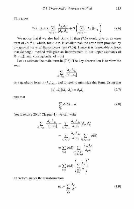
7.1 Chebycheff’s theorem revisited 115

This gives

��x� z� ≤ x ∑d1�d2≤z

&d1&d2�d1�d2�

+O( ∑d1�d2≤z

�&d1 ��&d2 �) (7.6)

We notice that if we also had �&d� ≤ 1� then (7.6) would give us an errorterm of O

(z2)� which, for z < x� is smaller than the error term provided by

the general sieve of Eratosthenes (see (7.3)). Hence it is reasonable to hopethat Selberg’s method will give an improvement to our upper estimates of��x� z�� and, consequently, of ��x�

Let us estimate the main term in (7.6). The key observation is to view thesum ∑

d1�d2≤z

&d1&d2�d1�d2�

as a quadratic form in �&d�d≤z� and to seek to minimize this form. Using that

�d1�d2��d1�d2�= d1d2 (7.7)

and that ∑��d��= d (7.8)

(see Exercise 20 of Chapter 1), we can write

∑d1�d2≤z

&d1&d2�d1�d2�

= ∑d1�d2≤z

&d1&d2d1d2

�d1�d2�

= ∑d1�d2≤z

&d1&d2d1d2

∑��d1�d2�

��

= ∑�≤z��

∑d1�d2≤z��d1�d2�

&d1&d2d1d2

= ∑�≤z��

⎛⎜⎝∑d≤z��d

&dd

⎞⎟⎠

2

Therefore, under the transformation

u� =∑d≤z��d

&dd� (7.9)


the initial quadratic form has been diagonalized to∑�≤z��u2�

Our next aim will be to minimize this new diagonal form, if possible.We recall that the sequence �&d� was chosen subject to the constraints that

&1 = 1 and &d = 0 for d > z Equation (7.9) tells us that we must also haveconditions on �u�� This can be seen by using the dual Mobius inversionformula (Theorem 1.2.3). We obtain

&��

=∑��d�

(d

�

)ud (7.10)

Thus we have the constraints

u� = 0 for any � > z

and ∑�<z

��u� = 1 (7.11)

Now we use (7.11) to write

∑�≤z��u2� =

∑�≤z��

(u�−

��

��V�z�

)2

+ 1V�z�

�

where

V�z� =∑d≤z

�2�d�

��d� (7.12)

From this expression we see immediately that the form∑�≤z��u2� has a

minimal value of 1/V�z�, attained at

u� =��

��V�z�

With the above choice of u�� and, consequently, with the choice

&� = �∑d≤z��d

��d/��d�

��d�V�z�(7.13)

of &�� we get

��x� z�≤ x

V�z�+O

( ∑d1�d2≤z

�&d1 ��&d2 �)

7.1 Chebycheff’s theorem revisited 117

It remains to analyze the O-error term above. Using (7.13) we obtain

V�z�&� = �∑d≤z��d

��d/��d�

��d�= �∑

t≤ z

�

��t��t�

��t�

= � ∑t≤ z

��t��=1

�2�t��

��t�= ��∏

p��

(1+ 1

p−1

) ∑t≤ z

��t��=1

�2�t�

��t�

This implies that

�V�z��&�� ≤ �V�z��and so

�&�� ≤ 1 for any �

Putting everything together finally gives:

Theorem 7.1.1

��x� z�≤ x

V�z�+O (

z2)

as x� z→� where V�z� =∑d≤z

�2�d�

��d�

Let us emphasize that, in the end, the sequence �&d� was well determinedby (7.13) and was not arbitrary. We could have given this definition right fromthe beginning, but in that way our choice would not have been motivated.

From Theorem 7.1.1 we can deduce now Chebycheff’s upper boundfor ��x�:

Corollary 7.1.2

��x�� x

logx

Proof We write, as usual,

��x�≤��x� z�+ zfor any z= z�x�≤ x� and use Theorem 7.1.1 to estimate ��x� z� To do this

we need to find a lower bound for∑d≤z

�2�d�

��d�and to choose an appropriate z

We have ∑d≤z

�2�d�

��d�≥∑d≤z

�2�d�

d=∑d≤z

1d−∑d≤z

′ 1d�


where the summation∑

d≤z′ is over non-squarefree integers d We recall that

we showed in Chapter 1 that

∑d≤z

1d= log z+O�1�

By combining this formula with the observation that

∑d≤z

′ 1d≤ 1

4

∑d≤ z

4

1d�

we then obtain ∑d≤z

�2�d�

��d�� log z

Hence

��x�� x

log z+ z2

Now we choose

z =(x

logx

)1/2

and get our desired estimate. �

Remark 7.1.3 The main terms

x∏p<z

(1− 1

p

)and

x∑d≤z

�2�d�

��d�

provided by the sieve of Eratosthenes and Selberg’s method, respectively,have the same order of magnitude. They are both O �x/ log z� However, theerror term provided by Selberg’s method is smaller than the Eratostheneserror term, and this is why we were now able to retrieve Chebycheff’s upperestimate for ��x�

7.2 Selberg’s sieve

In this section we formalize the method illustrated above. Let � be any finiteset of elements and let � be a set of primes. For each prime p ∈ �� let �p

be a subset of �. We denote by d squarefree numbers composed of primes

7.2 Selberg’s sieve 119

of � Let �1 =� and for squarefree integers d composed of primes of ��let �d = ∩p�d�p Let z be a positive real number and set

P�z� = ∏p∈�p<z

p

Denote by S�� z� the number of elements of

�\∪p�P�z��p

Theorem 7.2.1 (Selberg’s sieve, 1947)We keep the above setting and assume that there exist X > 0 and a multi-plicative function f�·� satisfying f�p� > 1 for any prime p ∈ �� such that forany squarefree integer d composed of primes of � we have

#�d =X

f�d�+Rd (7.14)

for some real number Rd We write

f�n�=∑d�nf1�d� (7.15)

for some multiplicative function f1�·� that is uniquely determined by f byusing the Mobius inversion formula; that is,

f1�n�=∑d�n��d�f

(nd

)

Also, we set

V�z� = ∑d≤zd�P�z�

�2�d�

f1�d�

Then

S�� z�≤ X

V�z�+O

⎛⎜⎝ ∑

d1�d2≤zd1�d2�P�z�

�R�d1�d2��⎞⎟⎠

To prove this theorem we will need the dual Mobius inversion formula andthe following generalization of (7.7):

Lemma 7.2.2 Let f be a multiplicative function and let d1�d2 be positivesquarefree integers. Then

f��d1�d2��f��d1�d2��= f�d1�f�d2�


Proof Exercise. �

Proof of Theorem 7.2.1 Let �&d� be any sequence of real numbers suchthat

&1 = 1

and

&d = 0 for any d > z

For a ∈�, let

D�a� = ∏p∈�a∈�p

p�

with the convention that D�a� = 1 if a �∈�p for any p ∈ � . Then

∑d�P�z�a∈�d

��d�= ∑d��P�z��D�a��

��d�≤( ∑d��P�z��D�a��

&d

)2

=⎛⎜⎝ ∑d�P�z�a∈�d

&d

⎞⎟⎠

2

(7.16)

Now let us look at the cardinality S�� z�. Using (7.16), we obtain

S�� z� = ∑a∈�

a��p∀p�P�z�

1= ∑d�P�z�

��d�∑a∈�d

1

= ∑a∈�

⎛⎜⎝ ∑d�P�z�a∈�d

��d�

⎞⎟⎠≤ ∑

a∈�

⎛⎜⎝ ∑d�P�z�a∈�d

&d

⎞⎟⎠

2

= ∑a∈�

⎛⎜⎜⎝ ∑d1�d2�P�z�a∈��d1�d2 �

&d1&d2

⎞⎟⎟⎠= ∑

d1�d2≤z&d1&d2#��d1�d2�

By (7.14) the above expression becomes

X∑


&d1&d2f��d1�d2��

+O⎛⎜⎝ ∑


�&d1 ��&d2 ��R�d1�d2��⎞⎟⎠

Here, the first sum is viewed as the main term of our estimates, while theO-sum is viewed as the error term. As in Section 7.1, we also view the main


term as a quadratic form in �&d�d≤z� which we seek to bring to a diagonalform and to minimize. By Lemma 7.2.2 and (7.14),

∑d1�d2�P�z�

&d1&d2f��d1�d2��

= ∑d1�d2≤zd1�d2�P�z�

&d1&d2f�d1�f�d2�

f��d1�d2��

= ∑d1�d2≤zd1�d2�P�z�

&d1&d2f�d1�f�d2�

∑��d1�d2�

f1��

= ∑�≤z��P�z�

f1��∑

d1�d2≤zd1�d2�P�z��d1�d2�

&d1&d2f�d1�f�d2�

= ∑�≤z��P�z�

f1��

⎛⎜⎜⎜⎝

∑d≤zd�P�z��d

&df�d�

⎞⎟⎟⎟⎠

2

Thus, under the transformation

u� =∑d≤zd�P�z��d

&df�d�

� (7.17)

our quadratic form is reduced to the diagonal form∑�≤z��P�z�

f1��u2� (7.18)

The dual Mobius inversion formula enables us to write

&�f��

= ∑d�P�z��d

�

(d

�

)ud� (7.19)

and so, by recalling that &d = 0 for d > z and &1 = 1� we obtain

u� = 0 for any � > z

and ∑�≤z��P�z�

��u� = 1


Then we can write, as before,

∑�≤z��P�z�

f1��u2� =

∑�≤z��P�z�

f1��

(u�−

��

f1��V�z�

)2

+ 1V�z�

�

from which we see immediately that the minimal value of the quadratic formgiven in (7.18) is 1/V�z� and is attained at

u� =��

f1��V�z� (7.20)

We note that here we have used that f1�p� = f�p�− 1 > 0 for any p ∈ ��hence, by the multiplicativity of f1�·�� that the coefficients f1�d� appearingin our form are positive.

It remains to analyze the error term

O

⎛⎜⎝ ∑


�&d1 ��&d2 ��R�d1�d2��⎞⎟⎠

More precisely, our aim is to find upper bounds for �&�� for all �≤ z��P�z�From (7.17) and (7.19) we obtain that for such �� we have

V�z�&� = f��∑d≤zd�P�z��d

� �d/��d�

f1��

= f�� ∑t≤ z

�t�P�z��t��=1

�2�t��

f1�t�f1��

= ��(∏p��

f�p�

f1�p�

) ∑t≤ z

�t�P�z��t��=1

�2�t�

f1�t�

= ��(∏p��

(1+ 1

f1�p�

)) ∑t≤ z

�t�P�z��t��=1

�2�t�

f1�t�

Therefore

�V�z��&�� ≤ �V�z��


and so

�&�� ≤ 1

Consequently, the error term becomes

O

⎛⎜⎝ ∑


�R�d1�d2��⎞⎟⎠ �

and this completes the proof of the theorem. �

In order to use Theorem 7.2.1 we need lower bounds for the quantity V�z�Useful bounds are given as follows.

Lemma 7.2.3 We keep the notation of Theorem 7.2.1. We let f �·� be thecompletely multiplicative function defined by f �p� = f�p� for all primes pand we set

P�z� = ∏p��p<z

p

Then

1. V�z�≥ ∑�≤z

p��⇒p�P�z�

1

f ��

2. f�P�z��V�z�≥ f1�P�z��∑�≤z

1

f ��

Proof

1. We want to express the quotients 1/f1�d� appearing in V�z� in terms ofthe function f For this, we observe that for d a squarefree integer suchthat d�P�z� we have

f�d�

f1�d�= ∏

p�d

f�p�

f1�p�=∏p�d

(1− 1

f�p�

)−1

= ∏p�d

∑n≥0

1f�p�n

=∑k

′ 1

f �k��

where the sum∑k

′is over integers k composed of prime divisors of d

Then

V�z�= ∑d≤zd�P�z�

��d�2

f�d�

∑k

′ 1

f �k�≥ ∑

�≤zp��⇒p�P�z�

1

f ��


2. Similarly to part 1, we write

f�P�z��

f1�P�z��V�z� = ∏

p��p<z

(1− 1

f�p�

)−1 ∑d≤zd�P�z�

��d�2

f�d�

∑k

′ 1

f �k�

= ∏p��p<z

(∑n≥0

1f�p�n

) ∑d≤zd�P�z�

��d�2

f�d�

∑k

′ 1

f �k�

≥ ∑�≤z

1

f �z�

�

7.3 The Brun–Titchmarsh theorem and applications

In this section we will use Selberg’s sieve to estimate the number of primesp≤ x in a given arithmetic progression. More precisely, for any given coprimeintegers a and k we will estimate

��x�k�a�= # �p ≤ x p≡ a�mod k��

The problem of studying the asymptotic behaviour of ��x�k�a� goes backto Legendre, who conjectured that given �a� k�= 1� there are infinitely manyprimes p such that p≡ a�mod k� It is also a particular case of Buniakowski’sconjecture concerning the prime values of integral valued polynomials.

In the late 1830s, Dirichlet proved Legendre’s conjecture by using importantproperties of certain generalizations of the Riemann zeta function (known asDirichlet L-functions). Dirichlet’s work on this problem is viewed now as thebeginning of analytic number theory. More precisely, Dirichlet showed thatthe analytic density of the set of primes p ≡ a�mod k� is 1/��k�� that is,that

lims→1

∑p≡a�mod k�

1/ps

log1/�s−1�= 1��k�

Actually, there is a more natural definition for the density of a set of primes:a set � of primes is said to have natural density � if the limit

limx→

# �p ≤ x p ∈ ��

# �p ≤ x�

exists and is equal to � It can be proven that if � has natural density �� thenit also has analytic density �� however the converse is not true in general.

7.3 The Brun–Titchmarsh theorem and applications 125

In the case of the set of primes p≡ a�mod k�� the natural density exists andthen, by Dirichlet’s theorem, we obtain the asymptotic formula

��x�k�a�∼ 1��k�

lix

Effective asymptotic formulae for ��x�k�a� are also known, as follows:

1. For any N > 0� there exists c�N� > 0 such that, if

k≤ �logx�N �then

��x�k�a�= 1��k�

lix+O (x exp

(−c�N��logx�1/2)) �uniformly in k (this is known as the Siegel–Walfisz theorem);

2. Assuming a generalized Riemann hypothesis (for Dirichlet L-functions)we have that, for any k≤ x�

��x�k�a�= 1��k�

lix+O (x1/2 log�kx�

)

The implied O-constant does not depend on k.

Thus, unconditionally, the error terms∣∣∣��x�k�a�− 1

��k�lix

∣∣∣ are known (only)

in a range of k < �logx�N Finally, the Bombieri–Vinogradov theoremmentioned in Section 3.3 of Chapter 3 allows us to control these error terms,on ‘average’ and unconditionally, in bigger ranges of k This important theo-rem will be discussed in detail in Chapter 9.

Our aim in this chapter is more modest than the results mentioned above.We want to obtain an upper bound for ��x�k�a� More precisely, we wantto prove:

Theorem 7.3.1 (The Brun–Titchmarsh theorem)

Let a and k be positive coprime integers and let x be a positive real numbersuch that k ≤ x� for some � < 1. Then, for any � > 0� there exists x0 =x0�� > 0 such that

��x�k�a�≤ �2+��x��k� log�2x/k�

for all x > x0


Proof We fix a positive real number z < x and observe that

��x�k�a� = ��z�k�a�+# �z≤ p ≤ x p≡ a�mod k��

≤ z+# �n≤ x n≡ a�mod k��n �≡ 0�mod p� ∀p < z� �p�k�= 1�

If we choose

� = �n≤ x n≡ a�mod k��

� = �p �p� k�= 1� �

and

�p = �n≤ x n≡ a�mod k��n≡ 0�mod p�� for all p ∈ ��

P�z� = ∏p<z

�p�k�=1

p�

then we have

S�� z�= # �n≤ x n≡ a�mod k��n �≡ 0�mod p� ∀p�P�z�� Hence once we obtain an upper bound for S�� z�� we also obtain anupper bound for ��x�k�a�

Since the primes p∈� are coprime to k� we can use the Chinese RemainderTheorem to deduce that

#�d =x

kd+O�1�

for any squarefree positive integer d composed of primes of �� where

�d = ∩p�d�p

Thus, in the notation of Theorem 7.2.1, we have X = x/k� f�d�= d�f1�d�=��d� and Rd = O�1�� and so

S�� z�≤ x

kV�z�+O (

z2)�

where

V�z� = ∑d≤z

�d�k�=1

�2�d�

��d�

Using part 2 of Lemma 7.2.3 together with formula (7.8), we obtain

k

��k�V�z�≥∑

�≤z

1�≥ log z+O�1�


Hence

��x�k�a�≤ z+S�� z�≤ x

��k��log z+O�1�� +O(z2)

By choosing

z =(2xk

) 12−�

for any arbitrary fixed 0 < � < 1� we get the desired upper estimate for��x�k�a� �

Remark 7.3.2 Montgomery and Vaughan [42] have proved the more preciseresult that

��x+y�k�a�−��x�k�a�≤ 2y��k� log�y/k�

for y > k. Any further improvement of the constant 2 in the above estimatewould imply the non-existence of Siegel zeros, as noted by several authorsbeginning with Chowla, Motohashi and Siebert. See [47] for a historicaldiscussion.

Following Erdos, we apply the Brun–Titchmarsh theorem, Brun’s sieve andthe sieve of Eratosthenes to the problem of finding an asymptotic formula forthe number of n ≤ x such that �n��n�� = 1. One can prove, using Sylowtheorems, that this is a necessary and sufficient condition for any group oforder n to be cyclic.

Theorem 7.3.3 (Erdos)The number of n≤ x such that �n��n��= 1 is

∼ e−�xlog log logx

as x→.

To prove this theorem, we will need the following preliminary results.

Lemma 7.3.4 Let 0< � < 1 and let p < �log logx�1−�. Then

∑′

q

1q>c1 log logx

p> �log logx��/2�

where the dash indicates that the sum is over primes q ≡ 1�mod p� satisfyingq < x1/�log logx�

2.


Proof Using the Siegel–Walfisz theorem stated above and partial summa-tion, we deduce the assertion of the lemma. �

Lemma 7.3.5 Let p be any prime. Then

∑q≤x

q≡1�mod p�

1q< c2

(log logx+ logp

p

)

Proof This follows from Theorem 7.3.1 and partial summation. �

Lemma 7.3.6 Let 0< � < 1 and let z ≤ �log logx�1+�. Then the number ofn≤ x not divisible by any prime p ≤ z is

�1+o�1��e−�xlog z

as x→.

Proof This is a simple application of the sieve of Eratosthenes. �

Lemma 7.3.7 Let 0< � < 1 and let p ≤ �log logx�1+�. Then the number ofn≤ x having the least prime divisor p is

�1+o�1�� e−�xp logp

as p→.

Proof This is a simple consequence of Lemma 7.3.6. �

Proof of Theorem 7.3.3 Let A�x� be the number of n ≤ x such that�n��n�� = 1. We partition these numbers into sets �p according to thesmallest prime divisor p of n� and we denote by Ap�x� the number of elementsin �p. Then

A�x�=∑p

Ap�x�=∑

1+∑

2+∑

3�

where in∑

1 we have p < �log logx�1−�, in

∑2 we have �log logx�

1−� < p <�log logx�1+�� and in

∑3 we have p > �log logx�

1+� for any fixed 0< �< 1


Observe that for each prime p� the numbers enumerated by Ap�x� do nothave any prime factor q ≡ 1�mod p�. By Brun’s sieve and Lemma 7.3.4,

Ap�x��x

p

∏q≡1�mod p�

q<x1/�log logx�2

(1− 1

q

)� x

pexp

(−�log logx��/2)

Therefore ∑1= o

(x

log log logx

)

For∑

2 we use Lemma 7.3.7 to deduce that

∑2� x

log log logx

∑′

p

1p�

where the dash on the sum indicates that �log logx�1−� < p < �log logx�1+�.We find ∑′

p

1p� ��

so that ∑2� �

x

log log logx

Finally, by the sieve of Eratosthenes,

∑3≤ �1+o�1�� e−�x

�1+�� log log logx �

since all the prime divisors of an n enumerated by∑

3 are greater than�log logx�1+�. On the other hand,

∑3≥ �1+o�1�� e−�x

�1+�� log log logx −∑p>y

x

p2−∑p>y

∑q≡1�mod p�pq≤x

x

pq�

where y = �log logx�1+�. The penultimate sum is easily seen to be

O

(x

log logx

)

The final sum is estimated using Lemma 7.3.5. It is

� x∑p>y

log logx+ logpp2

� x

�log logx��

by partial summation. This completes the proof. �


7.4 Exercises

1. Let f be a multiplicative function and let d1�d2 be positive squarefreeintegers. Then

f��d1�d2��f��d1�d2��= f�d1�f�d2�2. Use the method of Lagrange’s multipliers to find the minimal value of

the form ∑�≤z��P�z�

f1��u2�

defined in (7.18).3. Show that if a set of primes has natural density �� then it has analytic

density and this is also �4. Find an example of a set of primes that has analytic density, but does

not have natural density.5. Let a be a positive integer and x a positive real number. Show that, for

any A�B > 0�

∑xA

�logx�B≤k≤xA�logx�B�k�a�=1

��x�k�a�� x log logx�logx�2

6. For any natural number n recall that the radical of n is

rad�n� =∏p�np

Show that the number of n ≤ x such that rad�n� and ��rad�n�� arecoprime is

∼ e−�xlog log logx

as x→. (This gives an asymptotic formula for the number of n ≤ xsuch that all groups of order n are nilpotent. Since finite abelian groupsare nilpotent, we infer an asymptotic formula for the number of n ≤ xsuch that all groups of order n are abelian.) [Hint: modify the methodof proof of Theorem 7.3.3 to deduce the result.]

7. Using the Siegel–Walfisz theorem, show that

∑q<z

q≡1�mod d�

1q= log log z

��d�+O�1��

where the summation is over primes q ≡ 1�mod d�.

7.4 Exercises 131

8. In the previous exercise, show that if A is any positive number andd < �log z�A, then

∑q<z

q≡1�mod d�

1q= log log z

��d�+O

(logd��d�

)

9. For any positive integer d, show that

∑q<z

q≡1�mod d�

1q� log log z+ logd

��d�

10. Let

k�n� =∏p�n�n�p−1�

Show that ∑n≤x

logk�n�=(∑d

��d�

d��d�+o�1�

)x log logx

as x→. (k�n� is an upper bound for the number of non-isomorphicgroups of order n all of whose Sylow subgroups are cyclic.) [Hint:write

logk�n�=∑p�n

∑d�nd�p−1

��d��

and analyze the cases d < log logx and d > log logx separately, usingthe previous exercises.]

11. Fix � > 0. Let Hk�x� be the number of n ≤ x of the form n =p1p2 pkm, where all the pi are less than �log logx�1−�, all the primedivisors of m are greater than �log logx�1+� and �m��m�� = 1. Bymodifying the proof of Theorem 7.3.3, show that

Hk�x�∼e−�x�log log log logx�k

k! log log logxas x→.

12. By adapting the method of Theorem 7.3.3, show that the number ofn≤ x such that �n��n�� is prime is

∼ e−�x log log log logx

log log logx

[Hint: analyze the contribution from squarefree and non-squarefree nseparately.]


13. Prove that the number of n≤ x such that ��n��n��= k is

∼ e−�x�log log log logx�k

k! log log logxas x→. [Hint: proceed by induction on k and use the previous twoexercises.]

14. Prove that ∑d≤z

�2�d�

��d�≥ log z

[Hint: notice that the sum in question is

∑d≤z

�2�d�

d

∏p�d

(1− 1

p

)−1

= ∑rad�n�≤z

1n�

15. For positive integers k, define

Hk�x� =∑d≤x�d�k�=1

�2�d�

��d�

Show that

H1�x�=∑t�k

�2�t�

��t�Hk�x/t�

and deduce thatHk�x�

logx≥∏p�k

(1− 1

p

)

16. Let � be a set of natural numbers, � a set of primes, and for squarefreeintegers d composed of primes of � let �d be the set of elements of �divisible by d. Suppose that there exists X > 0 such that

#�d =X

d+Rd

for some real number Rd with �Rd� ≤ 1. Show that in this setting,Theorem 7.2.1 can be sharpened to

S�� z�≤ X

log z

∏p<zp��

(1− 1

p

)−1

+ z2

[Hint: use the previous exercise.]

7.4 Exercises 133

17. Let k be a natural number. Prove that the number of n ≤ x that arecoprime to k is

≤ x

log z

∏p≤z

�p�k�=1

(1− 1

p

)−1

+ z2�

for any z≤ x.18. Show that for z≤ x,

��x� z�≤ x

log z+ z2�

where ��x� z� is the number of n≤ x free of prime factors < z.19. Let k be a natural number and a an integer coprime to k. For k < y,

show that

��x+y�k�a�−��x�k�a�≤ 2y��k� log�y/k�

+O(

y

k log2�y/k�

)�

where the implied constant is absolute. (Using the large sieve,Montgomery and Vaughan [42] have shown that the error term abovecan be eliminated.)

20. Let �odd�x� z� (respectively �even�x� z�) denote the number of n ≤ xwith an odd (respectively even) number of prime factors, counted withmultiplicity, free of prime factors < z. Suppose that �d is a boundedsequence of real numbers satisfying∑

d�n��d�≤∑

d�n�d�

with �d = 0 for d > z. Let &�n� denote the Liouville function, whichis equal to �−1�r , where r is the total number of prime factors of ncounted with multiplicity. Assuming that∑

n≤x&�n�= O�x exp�−c�logx�1/2��

for some constant c > 0 (this assumption is equivalent to a strong formof the prime number theorem), show that, for any � < 1 and any z < x�,we have

�odd�x� z�≤x

2

∑d

�dd

+O�x�log z� exp�−c1�logx�1/2��

Establish a similar result for �even�x� z�. Deduce that

∑d≤√

x

�dd

≥ 2+o�1�logx


(This example, due to Selberg [59], shows the parity problem of thesieve method. As can be seen, the method gives the same bound for�even�x�

√x� and �odd�x�

√x�, whereas

�even�x�√x�= 0� �odd�x�

√x�= �1+o�1�� x

logx�

as x→. )

8The large sieve

The sieves discussed in the previous chapters rely on the use of the Möbiusfunction or of its variations (as in the case of Selberg’s sieve). They areclassified as ‘combinatorial sieves’. In this chapter we will discuss a sieve ofa completely different nature, called the large sieve, which was introducedby Yuri Linnik (1915–72) in 1941 and was subsequently improved by Rényi(1950), Roth (1965), Bombieri (1965), Davenport and Halberstam (1966),Gallagher (1967), and others. We refer the reader to [8, p. 151] for thehistory. This sieve can be deduced from a beautiful inequality, known as thelarge sieve inequality, which, at a first sight, does not seem to have the bigpotential that it actually has.

Linnik’s original motivation was to attack Vinogradov’s hypothesisconcerning the size of the least quadratic non-residue np�mod p�. Vinogradovconjectured that

np = O �p��for any � > 0 The generalized Riemann hypothesis implies

np = O(�logp�2

)

Linnik proved, using his large sieve, that the number of primes p ≤ x forwhich np > p

� is O �log logx� Linnik’s paper introduced a new theme inanalytic number theory that employed ideas from probability theory.

As will be seen in the following chapters, the large sieve has evolved intoa powerful tool, its significant application being the Bombieri–Vinogradovtheorem. The latter theorem has often served as a substitute for the use of thegeneralized Riemann hypothesis in certain contexts, and will be discussed indetail in the next chapter.

135

136 The large sieve

8.1 The large sieve inequality

We begin with a preliminary lemma.

Lemma 8.1.1 Let F �0�1�−→ � be a differentiable function with contin-uous derivative, extended by periodicity to all � with period 1. Let z be apositive integer. Then

∑d≤z

∑1≤a≤d�a�d�=1

∣∣∣F (ad

)∣∣∣≤ z2 ∫ 1

0�F��d�+

∫ 1

0�F ′��d� (8.1)

Proof Let d ≤ z, a ∈ �1�d�∩ with �a�d�= 1, and � ∈ �0�1�. Then

−F(ad

)=−F��+

∫ �

ad

F ′�t�dt

By taking absolute value on both sides, this implies∣∣∣F (ad

)∣∣∣≤ �F��+∫ �

ad

�F ′�t��dt (8.2)

Now let us fix � > 0 (to be chosen later) so that the intervals

I(ad

)=

(ad−�� a

d+�

)are contained in �0�1�. We integrate (8.2) over I �a/d�, with respect to �,and obtain

2�∣∣∣F (a

d

)∣∣∣≤ ∫I� ad �

�F��d�+∫I� ad �

∫ �

ad

�F ′�t��dt d� (8.3)

Since � ∈ I �a/d� and t ∈ �a/d��, we obtain that t ∈ I �a/d�. Hence theright-hand side of the above inequality is

≤∫I� ad �

�F��d�+∫I� ad �

∫I� ad �

�F ′�t��dt d�

=∫I� ad �

�F��d�+2�∫I� ad �

�F ′�t��dt

=∫I� ad �

�F��d�+2�∫I� ad �

�F ′��d�

In other words,

2�∣∣∣F (a

d

)∣∣∣≤ ∫I� ad �

�F��d�+2�∫I� ad �

�F ′��d� (8.4)

8.1 The large sieve inequality 137

Now we choose

� = 12z2

With this choice, the intervals I �a/d�, 1 ≤ a ≤ d� �a�d� = 1�d ≤ z do notoverlap (modulo 1). Indeed, let x ∈ I �a/d�∩ I �a′/d′� for a/d �= a′/d′. Then∣∣∣x− a

d

∣∣∣< ��∣∣∣∣x− a′d′

∣∣∣∣< ��and so ∣∣∣∣ad − a

′

d′

∣∣∣∣< 2�= 1z2 (8.5)

On the other hand, we have∣∣∣∣ad − a′

d′

∣∣∣∣= �ad′ −a′d�dd′

�= 0�

since if ad′ = a′d, then, recalling that �a�d�= �a′�d′�= 1, we obtain d= d′,which is false. Thus ∣∣∣∣ad − a

′

d′

∣∣∣∣≥ 1dd′

≥ 1z2 (8.6)

Putting together (8.5) and (8.6) we are led to a contradiction.We sum (8.4) over all intervals I �a/d� and get

1z2

∑d≤z

∑1≤a≤d�a�d�=1

∣∣∣F (ad

)∣∣∣ ≤ ∑I� ad �

∫I� ad �

�F��d�+ 1z2

∑I� ad �

∫I� ad �

�F ′��d�

≤∫ 1

0�F��d�+ 1

z2

∫ 1

0�F ′��d�

This completes the proof of the lemma. �

Now let us choose

F�� =(∑n≤xane�n��

)2

�

where �an�n≥1 is an arbitrary sequence of complex numbers, x is a positiveinteger and for a rational number t, e�t� = exp�2�it�

For simplicity of notation, set

S�� = ∑n≤xane�n��

138 The large sieve

hence

F��= S��2� F ′��= 2S��S′��

By Lemma 8.1.1 we obtain

∑d≤z

∑1≤a≤d�a�d�=1

∣∣∣S (ad

)∣∣∣2 ≤ z2 ∫ 1

0�S��2 d�+2

∫ 1

0�S��S′��d�

We now recall Parseval’s identity that

∫ 1

0

∣∣∣∣∣∑n≤xane�n��

∣∣∣∣∣2

d�= ∑n≤x

�an�2�

thus ∫ 1

0�S��2 d�= ∑

n≤x�an�2

This implies that

∑d≤z

∑1≤a≤z�a�d�=1

∣∣∣S (ad

)∣∣∣2 ≤ z2 ∑n≤x

�an�2+2∫ 1

0�S��S′��d�

For the second term on the right-hand side of the above inequality we use theCauchy–Schwarz inequality and, once again, Parseval’s identity. We obtain

∫ 1

0�S��S′��d� ≤

(∫ 1

0�S��2 d�

)1/2(∫ 1

0�S′��2 d�

)1/2

≤(∑n≤x

�an�2)1/2(∑

n≤x4�2n2�an�2

)1/2

≤ 2�x∑n≤x

�an�2

We record this result as:

Theorem 8.1.2 (The large sieve inequality)Let �an�n≥1 be a sequence of complex numbers and let x� z be positive integers.Then

∑d≤z

∑1≤a≤d�a�d�=1

∣∣∣∣∣∑n≤xane

(nad

)∣∣∣∣∣2

≤ (z2+4�x

)∑n≤x

�an�2� (8.7)

where, for a rational number �� e�� = exp�2�i��

8.2 The large sieve 139

Montgomery and Vaughan [42], and Selberg [60] have independently shownthat z2+4�x can be replaced by z2+x .

8.2 The large sieve

We want to deduce a sieve method from the inequality described inTheorem 8.1.2. Let � be a set of positive integers n≤ x and let � be a set ofprimes. For each p ∈ �� suppose that we are given a set

{w1�p� �w��p��p

}of ��p� residue classes modulo p Let z be a positive real number and denoteby P�z� the product of the primes p ∈ �� p < z We set

�� z� = {n ∈� n �≡ wi�p�mod p� ∀1≤ i ≤ ��p�� ∀p�P�z�} (8.8)

and we denote by S�� z� the cardinality of this set.

Theorem 8.2.1 (The large sieve)With the above notation, we have

S�� z�≤ z2+4�xL�z�

�

where

L�z� =∑d≤z�2�d�

∏p�d

��p�

p−��p�

The (unusual) idea for the proof of Theorem 8.2.1 is to use sums of theform

cd�n� =∑

1≤a≤d�a�d�=1

e(nad

)� (8.9)

where n�d ∈ , called Ramanujan sums. They have the following interestingproperties:

Proposition 8.2.2 Let d�d′ be positive integers. Then

1. if �d�d′�= 1� we have that cdd′�n�= cd�n�cd′�n��2. cd�n�=

∑D��d�n�

�

(d

D

)D�

3. if �d�n�= 1� we have that cd�n�= ��d�, that is,��d�= ∑

1≤a≤d�a�d�=1

e(nad

)

140 The large sieve

Proof Part 1 of the proposition is left to the reader as an exercise. Part 3 isa straightforward consequence of part 2. We now prove part 2.

Let

cd�n� =∑

1≤a≤de(nad

)

On one hand we can write

cd�n�= e(nd

) ∑0≤a≤d−1

e(nad

)�

and we see that this is e �n/d� e�n�−1e�n/d�−1 if d � n and e �n/d�d if d�n In other

words,

cd�n�={0 if d � n

d if d�n. (8.10)

On the other hand, we can write

cd�n� =∑D�d

∑1≤a≤d�a�d�=D

e(nad

)

= ∑D�d

∑1≤a1≤ d

D

�a1� dD �=1

e(nDa1d

)=∑D�dc dD�n�

By using the Möbius inversion formula we deduce that

cd�n�=∑D�d��D�c d

D�n�=∑

D�d�

(d

D

)cD�n��

which, by (8.10), is ∑D��d�n�

�

(d

D

)D

�

Proof of Theorem 8.2.1 First, let us set some notation. Let d= p1 pt be apositive squarefree integer composed of primes dividing P�z� By the ChineseRemainder Theorem, for any i= �i1� � it� with 1≤ i1 ≤��p1�� 1≤ it ≤��pt�� there exists a unique integer wi�d such that

wi�d ≡ wij�pj �mod pj� ∀1≤ j ≤ tWe denote by ��d� the number of all possible wi�d appearing in this fashion(namely, as we vary i, but keep d fixed). Clearly, ��d� is the product of the��pi�’s.

8.2 The large sieve 141

Now let n ∈ �� z� This implies that(n−wi�d�d

)= 1

for any d and i as above, and so by part 3 of Proposition 8.2.2 we obtain

��d�= cd(n−wi�d

)= ∑1≤a≤d�a�d�=1

e

((n−wi�d

)a

d

) (8.11)

We sum (8.11) over all indices i corresponding to d and over all integersn ∈ �� z� and get

��d��d�S�� z�= ∑1≤a≤d�a�d�=1

∑wi�d

e(−wi�da

d

) ∑n∈��z�

e(nad

) (8.12)

Squaring (8.12) out and applying the Cauchy–Schwarz inequality gives

��d��d�S�� z��2 ≤⎛⎜⎝ ∑

1≤a≤d�a�d�=1

∣∣∣∣∣∑wi�d

e(−wi�da

d

)∣∣∣∣∣2⎞⎟⎠

×⎛⎜⎝ ∑

1≤a≤d�a�d�=1

∣∣∣∣∣∑

n∈��z�e(nad

)∣∣∣∣∣2⎞⎟⎠

We write the first factor in the above expression as

∑1≤a≤d�a�d�=1

∑wi�d�wi′ �d

e

((wi′�d−wi�d

)a

d

)= ∑wi�d�wi′ �d

cd(wi′�d−wi�d

)�

and, further, by using part 2 of Proposition 8.2.2, as


∑D��d�wi�d−wi′ �d�

�

(d

D

)D = ∑

D�d


wi�d≡wi′ �d�mod D�

�

(d

D

)D

= ∑D�d�

(d

D

)D��d��

(d

D

)

= d��d�∑E�d

��E��E�

E

= d��d�∏p�d

(1− ��p�

p

)

= ��d�∏p�d�p−��p��

142 The large sieve

This gives us that

��d� ��d�S�� z��2

≤ ��d�∏p�d�p−��p��

⎛⎜⎝ ∑

1≤a≤d�a�d�=1

∣∣∣∣∣∑

n∈��z�e(nad

)∣∣∣∣∣2⎞⎟⎠ �

or, equivalently, that

�2�d�S�� z�2∏p�d

��p�

p−��p� ≤∑

1≤a≤d�a�d�=1

∣∣∣∣∣∑

n∈��z�e(nad

)∣∣∣∣∣2

(8.13)

Now we sum (8.13) over d≤ z and we use Theorem 8.1.2 with the sequence�an�n≥1 chosen such that an is 1 if n ∈ �� z� and 0 otherwise. We obtain

∑d≤z��d�2S�� z�2

∏p�d

��p�

p−��p� ≤(z2+4�x

)S�� z��

which, after doing the obvious cancelations, completes the proof of thetheorem. �

Remark 8.2.3 When using Theorem 8.2.1, we need lower bounds for thesum L�z� One way of obtaining a lower bound is by considering the summa-tion over primes p < z� and not over all integers d� that is,

L�z�≥∑p<z

��p�

p−��p�

In some situations, the lower bound obtained for L�z� in this manner issufficient, as in the case of applications to the Euclidean algorithm [29].

8.3 Weighted sums of Dirichlet characters

We want to exploit the large sieve inequality in a slightly different directionthan the one of the previous section.

We recall that for a positive integer d≥ 2, a (Dirichlet) character modulod is a group homomorphism � ��/d��∗ −→ �∗ One extends � to all of� by setting ��n�= 0 for any integer n not coprime to d This is a periodicfunction, whose values are �d−th roots of unity. The trivial (or principal)character modulo d, denoted �0, is defined by �0�n� = 1 for all n coprimeto d In the case that � is non-trivial and has period strictly less than d� we

8.3 Weighted sums of Dirichlet characters 143

say that it is an imprimitive character; otherwise, we say that it is primitive,of conductor d

An important result about Dirichlet characters, which will be useful inChapter 9, is that for any non-trivial character � modulo d,∑

M+1≤n≤M+N��n�� d

12 logd (8.14)

for any M�N This is known as the Pólya–Vinogradov inequality.There is an important function, called theGauss sum, which brings together

the character � modulo d and the exponential function e( ·d

)

�� = ∑1≤a≤d

��a�e(ad

)

One can show that if � is a primitive character modulo d� then

�� = d1/2 (8.15)

and, for �n�d�= 1,

��n�= 1� ��

∑1≤a≤d

��a�e(nad

)� (8.16)

where � denotes the complex conjugate of �We will use these two identitiesto obtain modified versions of the large sieve inequality.

Theorem 8.3.1 (First modified large sieve inequality)

Let �an�n≥1 be a sequence of complex numbers and let x� z be positive integers.Then

∑d≤z

d

��d�

∑�

∗∣∣∣∣∣∑n≤xan��n�

∣∣∣∣∣2

≤ (z2+4�x

)∑n≤x

�an�2� (8.17)

where the summation∑∗

�is over primitive characters � modulo d

Proof Let d ≤ z be fixed and let n be coprime to d. Let � be a primitivecharacter modulo d We multiply (8.16) by an� sum it over n ≤ x and thensquare it out. By using (8.15) we obtain∣∣∣∣∣

∑n≤xan��n�

∣∣∣∣∣2

= 1d

∣∣∣∣∣∑

1≤a≤d��a�

∑n≤xane

(and

)∣∣∣∣∣2

144 The large sieve

Now we sum the above identity over all primitive characters � modulo dand get

∑�

∗∣∣∣∣∣∑n≤xan��n�

∣∣∣∣∣2

= 1d

∑�

∗∣∣∣∣∣∑

1≤a≤d��a�

∑n≤xane

(and

)∣∣∣∣∣2

≤ 1d

∑�

∣∣∣∣∣∑

1≤a≤d��a�

∑n≤xane

(and

)∣∣∣∣∣2

= 1d

∑1≤a≤d

∑1≤b≤d

(∑n≤xane

(and

))(∑n≤xane

(bn

d

))∑�

��a��b��

where, for a complex number z� we denote by z its complex conjugate.By the orthogonality relations (see Exercise 3),

∑��a��b� is ��d� if

a≡ b�mod d� and 0 otherwise. Therefore

d

��d�

∑�

∗∣∣∣∣∣∑n≤xan��n�

∣∣∣∣∣2

≤ ∑1≤a≤d�a�d�=1

∣∣∣∣∣∑n≤xane

(and

)∣∣∣∣∣2

We sum over d ≤ z and apply the large sieve inequality to obtain (8.17). �

An immediate consequence of Theorem 8.3.1 and the Cauchy–Schwarzinequality is:

Corollary 8.3.2 Let �an�n≥1� �bm�m≥1 be sequences of complex numbers andlet x� y� z be positive integers. Then

∑d≤z

d

��d�

∑�

∗∣∣∣∣∣∑n≤x

∑m≤yanbm��nm�

∣∣∣∣∣≤ (z2+4�x

)1/2 (z2+4�y

)1/2(∑n≤x

�an�2)1/2(∑

m≤y�bm�2

)1/2

� (8.18)



We also want to prove a variation of (8.18) that will be very useful inChapter 9.

8.3 Weighted sums of Dirichlet characters 145

Theorem 8.3.3 (Second modified large sieve inequality)Let �an�n≥1� �bm�m≥1 be sequences of complex numbers and let x� y� z bepositive integers. Then

∑d≤z

d

��d�

∑�

∗maxu

∣∣∣∣∣∣∑n≤x

∑m≤ynm≤u

anbm��nm�

∣∣∣∣∣∣� (z2+x)1/2 (z2+y)1/2

(∑n≤x

�an�2)1/2(∑

m≤y�bm�2

)1/2

log�2xy�� (8.19)



Proof Clearly, in order to prove (8.19) we should make use of inequal-ity (8.18). To do this, we have to handle the condition nm ≤ u First weobserve that, without loss of generality, we can assume u= k+1/2 for someinteger 0 ≤ k ≤ xy Now let d ≤ z be fixed, let � be a primitive charactermodulo d, and let T > 0 By Exercise 17 with � = log�nm� and � = logu,we obtain ∑

n≤x

∑m≤ynm≤u

anbm��nm� =∫ T

−TA�t��B�t��

sin�t logu��t

dt

+O(1T

∑n≤x

∑m≤y

�anbm�∣∣log nmu

∣∣)� (8.20)

where

A�t�� = ∑n≤x

an��n�

nit� B�t�� = ∑

m≤y

bm��m�

mit

We note that, by our assumption on u� we have∣∣∣log nmu

∣∣∣� 1u� 1xy

and

sin�t logu��min �1� �t� log�2xy�� Then using the above in (8.20) gives∣∣∣∣∣∣

∑n≤x

∑m≤ynm≤u

anbm��nm�

∣∣∣∣∣∣ �∫ T

−T�A�t��B�t��min

{1�t� � log�2xy�

}dt

+ xyT

∑n≤x

∑m≤y

�anbm�

146 The large sieve

By applying the Cauchy–Schwarz inequality to the last sum, we get that∣∣∣∣∣∣∑n≤x

∑m≤ynm≤u

anbm��nm�

∣∣∣∣∣∣ �∫ T


{1�t� � log�2xy�

}dt

+ x3/2y3/2

T

(∑n≤x

�an�2)1/2(∑

m≤y�bm�2

)1/2

We take the maximum over u and then sum over � and d ≤ z to obtain

∑d≤z

d

��d�

∑�

∗maxu

∣∣∣∣∣∣∑n≤x

∑m≤ynm≤u

anbm��nm�

∣∣∣∣∣∣�∑

d≤z

d

��d�

∑�

∗ ∫ T


{1�t� � log�2xy�

}dt

+x3/2y3/2

T

∑d≤z

d

��d�

∑�

∗(∑n≤x

�an�2)1/2(∑

m≤y�bm�2

)1/2

(8.21)

Now we use the Cauchy–Schwarz inequality, Corollary 8.3.2 and Exercise15 to obtain upper bounds for the first term on the right-hand side of (8.21):

∑d≤z

d

��d�

∑�

∗ ∫ T


{1�t� � log�2xy�

}dt

≤⎛⎝∑d≤z

d

��d�

∑�

∗∣∣∣∣∣∑n≤xan��n�

∣∣∣∣∣2⎞⎠

1/2⎛⎝∑d≤z

d

��d�

∑�

∗∣∣∣∣∣∑m≤ybm��m�

∣∣∣∣∣2⎞⎠

1/2

×∫ T

−Tmin

{1�t� � log�2xy�

}dt

≤ (z2+4�x

)1/2 (z2+4�y

)1/2(∑n≤x

�an�2)1/2(∑

m≤y�bm�2

)1/2

× �logT + log�2xy�� (8.22)

For the second term on the right-hand side of (8.21) we observe that thereare ��d� characters modulo d (see Exercise 4), hence

x3/2y3/2

T

∑d≤z

d

��d�

∑�

∗(∑n≤x

�an�2)1/2(∑

m≤y�bm�2

)1/2

≤ x3/2y3/2z2

T

(∑n≤x

�an�2)1/2(∑

m≤y�bm�2

)1/2

(8.23)

8.4 An average result 147

Putting together (8.21), (8.22) and (8.23), and choosing T = x3/2y3/2 givesthe desired inequality. �

8.4 An average result

In this section we deduce an average result of Barban, Davenport andHalberstam about the behaviour of the error term in the prime number theoremfor primes in an arithmetic progression.

Let x be a positive real number and a�d integers with �a�d� = 1 Bypartial summation, in order to study ��x�d�a� it is actually enough to studythe function

��x�d�a� = ∑n≤x

�a�n�=1

��n�� (8.24)

where ��·� is the von Mangoldt function. Hence our focus in this section willbe on the function ��x�d�a� instead of ��x�d�a�.

Theorem 8.4.1 (The Barban–Davenport–Halberstam theorem)For any A > 0 and for any z satisfying x/�logx�A ≤ z≤ x� we have

∑d≤z

∑1≤a≤d�a�d�=1

∣∣∣∣��x�d�a�− x

��d�

∣∣∣∣2

≤ xz logx

Proof We start by rewriting the error term ��x�d�a�−x/��d� in a moreconvenient form. Namely, for any d ≤ z and 1 ≤ a ≤ d with �a�d�= 1� weobserve that

��x�d�a�= 1��d�

∑��mod d�

��a��x��


��mod d�is over (not necessarily primitive) Dirichlet

characters � modulo d� and where

��x�� = ∑n≤x��n��n� (8.25)

Let �0 denote the trivial character modulo d. We observe that

��x�d�a�− x

��d�= 1��d�

∑��mod d�� =�0

��a��x��+ ��x��0�−x��d�

(8.26)

148 The large sieve

By using the orthogonality relations, we see that

∑1≤a≤d�a�d�=1

∣∣∣∣∣∣∣∑

��mod d�� =�0

��a��x��

∣∣∣∣∣∣∣2

= ��d� ∑��mod d�� =�0

��x��2 (8.27)

Now let us remark that if the character � �= �0 modulo d is induced by someprimitive character �1 modulo d1� then

��x��= ��x��1�+O ��logx��logd�� (8.28)

Indeed, we have

��x��1�−��x��=∑pk≤xp�d

�1(pk

)logp� ∑

p≤xp�d

[logxlogp

]logp� �logx��logd�

Hence, by using (8.26), (8.27) and (8.28), we get

∑d≤z

∑1≤a≤d�a�d�=1

∣∣∣∣��x�d�a�− x

��d�

∣∣∣∣2

�∑d≤z

1��d�

∑��mod d�� =�0

��x��2+∑d≤z

1��d�

��x��0�−x�2

�∑d≤z

1��d�

∑��mod d�� =�0

��x��1��2+∑d≤z

1��d�

��x�−x�2+ z�log z�2�logx�2�

where ��x� is defined in (1.3) of Chapter 1.Let us remark that the second term above can be estimated using the

following form of the prime number theorem:

��x�= x+O(x exp

(−c√logx

))(8.29)

for some c > 0 (see [8, Chapter 18]). Thus

∑d≤z

1��d�

��x�−x�2 � x2 log z�logx�A

� xz logx�

where A > 0 is as in the statement of the theorem.

8.4 An average result 149

Since the term z�log z�2�logx�2 is negligible compared to the desired finalestimate of xz logx� we now see that in order to prove the theorem it sufficesto show that

∑d≤z

1��d�

∑��mod d�� =�0

��x��1��2 � xz logx (8.30)

For each character � �= �0 modulo d and its associated primitive character�1 modulo d1� let us write d = d1k for some positive integer k We have

∑d≤z

1��d�

∑��mod d�� =�0

��x��1��2

= ∑d1≤z

∑�1�mod d1�

��x��1��2∑k≤ z

d1

1��d1k�

=∑d≤z

∑�

∗ ��x��2 ∑k≤ z

d

1��dk�

�


�is over primitive characters � modulo d.

We observe that the innermost sum satisfies (see Exercise 15)

∑k≤ z

d

1��dk�

� 1��d�

log2zd

Therefore, in order to prove (8.30) it is enough to show that

∑d≤z

1��d�

log(2zd

)∑�

∗ ��x��2 � xz logx (8.31)

To do this, we remark that, by the first modified large sieve inequalityapplied to the sequence an =��n�� we have

∑d≤z

d

��d�

∑�

∗ ��x��2 � (z2+x)x logx� (8.32)

since∑

n≤x ��n�2 � x logx (see Exercise 13 of Chapter 1).

We will now use this estimate in a slightly indirect manner. More precisely,letD=D�x� be a parameter to be chosen later and such that 1<D≤ z� and letus divide the interval �D� z� into dyadic subintervals �U�2U� with U = z/2k�

150 The large sieve

where k are integers running from 1 to log�z/D�/ log2. By (8.32) togetherwith partial summation, we are led to

∑U<d≤2U

1��d�

log(2zd

)∑�

∗ ��x��2

�(x2

U+Ux

)�logx� log

(2zU

)

for each interval �U�2U� Now we sum over all U = z/2k and obtain

∑D<d≤z

1��d�

log(2zd

)∑�

∗ ��x��2 � x2

D�logx�2+ zx logx (8.33)

If we choose

D = �logx�A+1 (8.34)

and if we recall that x/�logx�A ≤ z≤ x� then (8.33) becomes

∑D<d≤z

1��d�

log(2zd

)∑�

∗ ��x��2 � zx logx (8.35)

In order to complete the proof of (8.30), it remains to show that

∑2≤d≤D

1��d�

log(2zd

)∑�

∗ ��x��2 � zx logx (8.36)

With D as in (8.34) and for any non-trivial character � modulo d such thatd ≤ D� the Siegel–Walfisz theorem stated in Section 7.3 of Chapter 7 givesthat

��x�� x exp(−c√logx

)(8.37)

for some positive constant c = c�A� (see Exercise 12). Therefore

∑2≤d≤D

1��d�

log(2zd

)∑�

∗ ��x��2

�D�log z�x2 exp(−2c

√logx

)

� x2

�logx�A� zx logx

This proves (8.36) and also completes the proof of the theorem. �

8.5 Exercises 151

8.5 Exercises

1. (Parseval’s identity) Let �an�n≥1 be complex numbers and x be apositive integer. Show that

∫ 1

0

∣∣∣∣∣∑n≤xane�n��

∣∣∣∣∣2

d�= ∑n≤x

�an�2�

where e�n��= exp�2�in��2. Let d�d′� n be positive integers. Show that, if �d�d′�= 1� then

cdd′�n�= cd�n�cd′�n��where cd�n� is defined in (8.9).

3. (The orthogonality relations) Let � denote Dirichlet characters modulod Then

∑�

��a��b�={��d� if a≡ b�mod d�

0 if a �≡ b�mod d�

and

∑n�mod d�

��n�={��d� if � = �00 if � �= �0

4. Show that there are exactly ��d� Dirichlet characters modulo d5. Let � be a Dirichlet character modulo d If � is imprimitive, show that

there exist a proper factor d1 of d and a primitive character �1 modulod1 such that

��n�={�1�n� if �n�d�= 1

0 if �n�d� > 1

6. Let � be a primitive character modulo d Show that, for any integer n�

��n�� = ∑1≤a≤d

��a�e(nad

)

Deduce that

��n��2 �� 2 = ∑1≤a1≤d

∑1≤a2≤d

��a1��a2�e(n�a1−a2�

d

)

7. Use the previous exercise to show that, if � is a primitive charactermodulo d� then

�� = d1/2

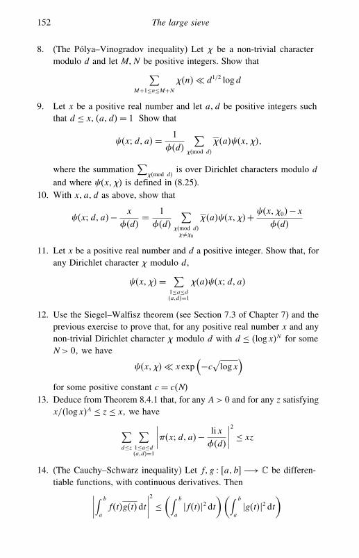
152 The large sieve

8. (The Pólya–Vinogradov inequality) Let � be a non-trivial charactermodulo d and let M�N be positive integers. Show that∑

M+1≤n≤M+N��n�� d1/2 logd

9. Let x be a positive real number and let a�d be positive integers suchthat d ≤ x� �a�d�= 1 Show that

��x�d�a�= 1��d�

∑��mod d�

��a��x��


��mod d�is over Dirichlet characters modulo d

and where ��x�� is defined in (8.25).10. With x�a�d as above, show that

��x�d�a�− x

��d�= 1��d�

∑��mod d�� =�0

��a��x��+ ��x��0�−x��d�

11. Let x be a positive real number and d a positive integer. Show that, forany Dirichlet character � modulo d�

��x��= ∑1≤a≤d�a�d�=1

��a��x�d�a�

12. Use the Siegel–Walfisz theorem (see Section 7.3 of Chapter 7) and theprevious exercise to prove that, for any positive real number x and anynon-trivial Dirichlet character � modulo d with d ≤ �logx�N for someN > 0� we have

��x�� x exp(−c√logx

)for some positive constant c = c�N�

13. Deduce from Theorem 8.4.1 that, for any A> 0 and for any z satisfyingx/�logx�A ≤ z≤ x� we have

∑d≤z

∑1≤a≤d�a�d�=1

∣∣∣∣��x�d�a�− lix��d�

∣∣∣∣2

≤ xz

14. (The Cauchy–Schwarz inequality) Let f� g �a� b� −→ � be differen-tiable functions, with continuous derivatives. Then∣∣∣∣

∫ b

af�t�g�t�dt

∣∣∣∣2

≤(∫ b

a�f�t��2 dt

)(∫ b

a�g�t��2 dt

)

8.5 Exercises 153

15. Let z be a positive real number and d a positive integer. Show that

∑k≤ z

d

1��dk�

� 1��d�

log2zd

16. Let y > 0� c > 0� T > 0�

��y� =

⎧⎪⎪⎨⎪⎪⎩0 if 0< y < 1

1/2 if y = 1

1 if y > 1�

and

I�y�T� = 12�i

∫ c+iT

c−iTys

sds

Show that

�I�y�T�−��y��<⎧⎨⎩y

cmin(1� 1

T � logy�)

if y �= 1cT

if y = 1

17. Use the previous exercise to show that, for any T > 0�� ∈ �� > 0�we have

∫ T

−Teit�

sin�t��t

dt =

⎧⎪⎪⎨⎪⎪⎩�+O

(1

T��−��)

if ��< ��2 if �� = �O(

1T��−��

)if ��> �

18. Let T > 0 and x� y be positive integers. Show that

∫ T

−Tmin

(1�t� � log�2xy�

)dt = O �logT + log�2xy��

19. Let � be a set of Z integers. Let p be a prime and set

S

(a

p

)= ∑

n∈�e(na

p

)�

where, as before, e�t� = exp�2�it�. Let Z�p�h� be the number ofelements of � that are ≡ h (mod p). Show that

∑�a�p�=1

∣∣∣∣S(a

p

)∣∣∣∣2

= p ∑h�modp�

(Z�p�h�− Z

p

)2

154 The large sieve

20. With notation as in the previous exercise, let d be an arbitrary positiveinteger and set

S(ad

)= ∑

n∈�e(nad

)

Let Z�d�h� be the number of elements of � that are ≡ h�mod d�. Let

T�d�h� = ∑�a�d�=1

S(ad

)e(−ahd

)

Prove that

dZ�d�h�=∑��dT

(d

��h

)

Deduce that

∑�a�d�=1

∣∣∣S (ad

)∣∣∣2 = d d∑h=1

(∑��d

��

�Z

(d

��h

))2

21. Let

S(ad

)= ∑

n∈�ane

(nad

)�

where � is a finite set of integers. For p prime, let

S�p�a� = ∑n∈�

n≡a�mod p�

an

and let ��p� be the number of a�mod p� for which S�p�a� = 0. Byobserving that

S�0�=p∑a=1

S�p�a�

and using the Cauchy–Schwarz inequality, show that

�S�0��2(��p�

p−��p�)≤ ∑�a�p�=1

∣∣∣∣S(a

p

)∣∣∣∣2

22. We keep the notation of the previous exercise. Let d1�d2 be coprimepositive integers, and let d = d1d2. Observing that by the Chineseremainder theorem we have

∑�a�d�=1

∣∣∣S (ad

)∣∣∣2 = ∑�a1�d1�=1

∑�a2�d2�=1

∣∣∣∣S(a1d1

+ a2d2

)∣∣∣∣2

�

8.5 Exercises 155

deduce that ∑�a�d�=1

∣∣∣S (ad

)∣∣∣2 ≥ �S�0��2J�d1�J�d2��

where

J�d� =∏p�d

��p�

p−��p�

Then deduce that∣∣∣∣∣∑n∈�an

∣∣∣∣∣2

�2�d�∏p�d

��p�

p−��p� ≤∑

�a�d�=1

∣∣∣S (ad

)∣∣∣2 (This gives an alternate method for deriving Theorem 8.2.1.)

9The Bombieri–Vinogradov theorem

The Bombieri–Vinogradov theorem is considered one of the finest conse-quences of the large sieve method. Its virtue lies in the fact that in many ques-tions that require the use of the generalized Riemann hypothesis for DirichletL-functions, one can apply the Bombieri–Vinogradov theorem. Thus, in situ-ations involving ‘sufficiently many’ L-functions, the theorem can be regardedas a substitute for the generalized Riemann hypothesis. As we will see below,one application is to the Titchmarsh divisor problem. Another more compli-cated application can be found in Hooley’s monograph [31], where an asymp-totic formula is derived for the number of ways of writing a natural numberas the sum of a prime number and two squares.

In 1976, Motohashi [43] discovered an induction principle that generalizesthe Bombieri–Vinogradov theorem and makes it applicable in a wider contextfor general arithmetical functions. This perspective was useful in the workof Bombieri et al. [2, 3], where the range of summation in the classicalBombieri–Vinogradov theorem is extended beyond the

√x barrier. We refer

the reader to Section 12 of [1], where a brief discussion of the new ideas canbe found.

In this chapter we will derive the classical Bombieri–Vinogradov theoremusing a method of Vaughan, as described in [8]. We show that the methodhas a wide range of applicability by putting it in a general context. We thenapply the results to treat the Titchmarsh divisor problem. In the next chapter,we will use the Bombieri–Vinogradov theorem in conjunction with the lowerbound sieve method to count the number of primes p such that p+ 2 hasa bounded number of prime factors, a result that represents some advancetowards the twin prime conjecture.

156

9.1 A general theorem 157

9.1 A general theorem

The main result of this section is derived as a generalization of a method ofVaughan, which lies at the heart of one proof of the celebrated Bombieri–Vinogradov theorem.

Before stating the general result, let us introduce the class of functions

� ={D −→ �

∑n≤x

�D�n��2 = O �x�logx�� for some � > 0

} (9.1)

We have the following basic properties:

Proposition 9.1.1

1. If D ∈� and � ≥ 0� then

∑n≤x

�D�n��n�

� x1−��logx��

for some � > 0

2. If D1�D2 ∈�� then∑ef≤x

�D1�e�D2�f ��d�ef �� x�logx��

for some � > 0� and∑ef≤x

�D1�e�D2�f ��2d�ef �� x�logx��

for some � > 0� where for a positive integer e, d�e� denotes the numberof the divisors of e

Proof Exercise. �

Theorem 9.1.2 Let x� z be positive integers and let

A�s�= ∑n≥1

a�n�

ns� B�s�= ∑

n≥1

b�n�

ns

be normalized Dirichlet series (that is, a�1�= b�1�= 1) for which we write

A�s�

B�s�= ∑n≥1

c�n�

ns�

1B�s�

= ∑n≥1

b�n�

ns

158 The Bombieri–Vinogradov theorem

for some c�n�� b�n� ∈ � We assume that all these series are convergent forRe�s� > "0 for some "0� and that they satisfy the following hypotheses:

(H1) �a�n��n≥1 is an increasing sequence of positive real numbers;(H2) b�·�� b�·�� c�·� ∈��(H3) there exist 0 ≤ � < 1 and 0 ≤ � < 1 such that, for any non-trivial

Dirichlet character � modulo d,∑n≤xb�n��n�� x�

√d logd+x�

Then

1. if z≤ x 1−�3−� �

∑d≤z

d

��d�

∑�

∗maxy≤x

∣∣∣∣∣∑n≤yc�n��n�

∣∣∣∣∣ (9.2)

�(z2x

12 +x+ zx 5−�

2�3−�� + z2x 1−�+2�3−� + z 5

2 x1+�3−� a�x�

)�logx��

′

for some �′ > 0�2. if z > x

1−�3−� �

∑d≤z

d

��d�

∑�

∗maxy≤x

∣∣∣∣∣∑n≤yc�n��n�

∣∣∣∣∣ (9.3)

�(z2x

12 +x+ z 9−4�

2�3−2�� x2−�3−2� a�x��log z�

+ z 3−4�+3�3−2� x

2−2�+�3−2� �log z�

)�logx��

′′

for some �′′ > 0

Here, the summation∑∗

�is over primitive Dirichlet characters � modulo d

Proof We set

F�s� = ∑n≤U

c�n�

ns� G�s� = ∑

n≤V

b�n�

ns

for some parameters U =U�x� z� and V =V�x� z�, to be chosen later. We thinkof F�s� as an ‘approximation to A�s�/B�s�’ and of G�s� as ‘an approximationto 1/B�s�’, and we observe that we can write

A�s�

B�s�= F�s�−B�s�G�s�F�s�+A�s�G�s�

+(A�s�

B�s�−F�s�

)�1−B�s�G�s�� (9.4)


In the literature, this is known as Vaughan’s identity and goes back to ideasof Linnik. By comparing the coefficients of n−s on both sides of (9.4), wededuce that

c�n�= a1�n�+a2�n�+a3�n�+a4�n��where

a1�n� ={c�n� if n≤ U0 if n > U�

(9.5)

a2�n� =−∑efg=nf≤Vg≤U

b�e�b�f �c�g�� (9.6)

a3�n� =∑ef=nf≤V

a�e�b�f �� (9.7)

a4�n� =−∑ef=ne>Uf>V

c�e�∑gh=fh≤V

b�g�b�h� (9.8)

Therefore, for any Dirichlet character � modulo d we can write∑n≤yc�n��n�= ∑

1≤i≤4

∑n≤yai�n��n�=

∑1≤i≤4

Si�y�� (9.9)

We prove the theorem by estimating each of the sums

∑d≤z

d

��d�

∑�

∗maxy≤x �Si�y�� 1≤ i ≤ 4

The estimate for S1�y�� Using (9.5) and hypothesis (H2) together withpart 1 of Proposition 9.1.1, we obtain

�S1�y�� =∣∣∣∣∣∣∑n≤yn≤U

c�n��n�

∣∣∣∣∣∣�∑n≤U

�c�n�� U�logU��0

for some �0 > 0 The above bound is independent of y�� and d� hence,recalling that there are ��d� Dirichlet characters modulo d, we obtain

∑d≤z

d

��d�

∑�

∗maxy≤x �S1�y�� z2U�logU��0 (9.10)


The estimate for S2�y�� Using (9.6) we write

S2�y��=− ∑efg≤yf≤Vg≤U

b�e�b�f �c�g��efg��

which we split into two parts according to whether fg ≤ U or U < fg ≤ UVThe first sum obtained in this way will be denoted by S′2�y�� and the secondsum by S′′2 �y��For S′2�y�� we write

�S′2�y�� ≤∑g≤U

�c�g�� ∑f≤min�V� Ug �

∣∣b�f �∣∣∣∣∣∣∣∣∑e≤ y

fg

b�e��e�

∣∣∣∣∣∣so that we can use hypothesis (H3) to estimate the innermost sum. We get

S′2�y�� y�√d�logd�

∑g≤U

�c�g��g�

∑f≤min�V� Ug �

∣∣b�f �∣∣f�

+y� ∑g≤U

�c�g��g�

∑f≤min�V� Ug �

∣∣b�f �∣∣f�

� y�√d�logd�

∑g≤U

�c�g��g�

∑f≤ U

g

∣∣b�f �∣∣f�

+y� ∑g≤U

�c�g��g�

∑f≤ U

g

∣∣b�f �∣∣f�

Then, by using (H2) and part 1 of Proposition 9.1.1, we obtain

S′2�y�� y�√d�logd�

∑g≤U

�c�g��g�

(U

g

)1−��logU��1

+y� ∑g≤U

�c�g��g�

(U

g

)1−��logU��2

� y�√d�logd�U 1−��logU��3 +y�U 1−��logU��4

for some �1��2��3��4 > 0 This implies that

∑d≤z

d

��d�

∑�

∗maxy≤x �S′2�y��

� x�z52 �log z�U 1−��logU��3 +x�z2�log z�U 1−��logU��4 (9.11)


For S′′2 �y�� we write

∑d≤z

d

��d�

∑�

∗maxy≤x �S′′2 �y��

=∑d≤z

d

��d�

∑�

∗maxy≤x

∣∣∣∣∣∣∣∑eh≤y

U<h≤UV

b�e�

⎛⎜⎝ ∑f≤V�g≤Ufg=h

b�f �c�g�

⎞⎟⎠��eh�

∣∣∣∣∣∣∣ �which suggests that we use the second modified large sieve inequality discussedin Chapter 8. However, we observe that by applying this inequality directlyto the pair of sequences of complex numbers

�b�e�� xUV <e≤ x

Uand

(b�f �c�g�

)fg=h�U<h≤UV

�

we will overestimate our expression. Instead, we should divide the interval�U�UV� into dyadic intervals �2k�2k+1� with �log2U� < k < �log2UV� andapply the modified large sieve inequality to each of the pair of sequences

�b�e�� x

2k+1 <e≤ x

2kand

(b�f �c�g�

)fg=h�2k<h≤2k+1

For each �log2U� < k < �log2UV� we obtain that

∑d≤z

d

��d�

∑�

∗maxy≤x

∣∣∣∣∣∣∣∑eh≤y

2k<h≤2k+1

b�e�


b�f �c�g�

⎞⎟⎠��eh�

∣∣∣∣∣∣∣�

(z2+ x

2k

)1/2 (z2+2k

)1/2(∑e

′)1/2(∑

h

′)1/2

�logx�� (9.12)

where

∑e

′= ∑

e≤ x

2k

�b�e��2� (9.13)

∑h

′= ∑

2k<h≤2k+1

∣∣∣∣∣∣∣∑

f≤V�g≤Ufg=h

b�f �c�g�

∣∣∣∣∣∣∣2

(9.14)

By (H2) we get ∑e≤ x

2k

�b�e��2 � x

2k

(log

x

2k

)�5(9.15)


for some �5 > 0� and by the Cauchy–Schwarz inequality together with (H2)and part 2 of Proposition 9.1.1, we get

∑2k<h≤2k+1

∣∣∣∣∣∣∣∑

f≤V�g≤Ufg=h

b�f �c�g�

∣∣∣∣∣∣∣2

� ∑2k<h≤2k+1

d�h�∑f �h

∣∣b�f �∣∣2 ∣∣∣∣c(h

f

)∣∣∣∣2

� 2k(log2k

)�6 (9.16)

for some �6 > 0 Then we plug (9.15) and (9.16) into (9.13), (9.14), (9.12),to obtain

∑d≤z

d

��d�

∑�

∗maxy≤x

∣∣∣∣∣∣∣∑eh≤y

2k<h≤2k+1

b�e�


b�f �c�g�

⎞⎟⎠��eh�

∣∣∣∣∣∣∣�

(z2+ zx

1/2

2k/2+ z2k/2+x1/2

)x

12 �logx�

�52 +1

(log2k

) �62

We sum over all k to finally get

∑d≤z

d

��d�

∑�

∗maxy≤x �S′′2 �y�� (9.17)

�(z2+ zx

1/2

U 1/2+ z�UV�1/2+x1/2

)x

12 �logx�

�52 +1�logUV�

�62 +1

The estimate for S3�y�� We define a step function � � −→ � by��t�= a�1� if t ≤ 1� ��t�= a�2�−a�1� if 1< t ≤ 2� and, generally, ��t�=a�n�−a�n−1� if n−1< t ≤ n Then we observe that a�n�= ∫ n

0 ��t�dt andthat ��·� is positive, since the sequence �a�n��n≥1 is increasing. Using (9.7)(and assuming, without loss of generality, that y is an integer) we write

�S3�y�� =∣∣∣∣∣∣∑f≤Vb�f ��f �

∑e≤ y

f

a�e��e�

∣∣∣∣∣∣=

∣∣∣∣∣∣∑f≤Vb�f ��f �

∑e≤ y

f

��e�∫ e

0��t�dt

∣∣∣∣∣∣


=∣∣∣∣∣∣∫ y

0��t�

∑f≤Vb�f ��f �

∑t≤e≤ y

f

��e�dt

∣∣∣∣∣∣≤

∫ y

0��t�� ∑

f≤V

∣∣b�f �∣∣∣∣∣∣∣∣∑t≤e≤ y

f

��e�

∣∣∣∣∣∣ dtWe remark that we can use the Pólya–Vinogradov inequality (8.14) to estimatethe inner sum. We obtain

S3�y��√d�logd�

∫ y

0��t��dt∑

f≤V

∣∣b�f �∣∣�√d�logd�V�logV��7a�y�

for some �7 > 0 Therefore, by observing that ��t�� = ��t� and by using(H1), we further obtain

∑d≤z

d

��d�

∑�

∗maxy≤x �S3�y�� z

52 �log z�V�logV��7 max

y≤x �a�y��

= z52 �log z�V�logV��7a�x� (9.18)

The estimate for S4�y�� By using (9.8) we write

∑d≤z

d

��d�

∑�

∗maxy≤x �S4�y��

=∑d≤z

d

��d�

∑�

∗maxy≤x

∣∣∣∣∣∣∣∣∑ef≤ye>Uf>V

c�e�

⎛⎜⎝∑gh=fh≤V

b�g�b�h�

⎞⎟⎠��ef �

∣∣∣∣∣∣∣∣�

which suggests that we apply the second modified large sieve inequality tothe pair of sequences of complex numbers

�c�e��U<e< xV

and(b�g�b�h�

)gh=f�h≤V�V<f< x

U

However, in order to obtain optimal results, we proceed as when handlingthe sum S′′2 �y�� To be precise, we divide the interval �U� y/V � into dyadicintervals

(2k�2k+1

]with �log2U� < k≤ �log2 y/V � and we apply the modified

large sieve inequality to each of the pair of sequences

�c�e��2k<e≤2k+1 and(b�g�b�h�

)gh=f�h≤V�max�V� y

2k+1 �<f<y

2k


For each �log2U� < k≤[log2

y

V

]we obtain

∑d≤z

d

��d�

∑�

∗maxy≤x

∣∣∣∣∣∣∣∣∣∣∣∑ef≤ye>Uf>V

2k<e≤2k+1

c�e�


b�g�b�h�

⎞⎟⎠��ef �

∣∣∣∣∣∣∣∣∣∣∣� (z2+2k

)1/2 (z2+ x

2k

)1/2(∑

e

′′)1/2(∑

f

′′)1/2

logx� (9.19)

where ∑e

′′= ∑

2k<e≤2k+1

�c�e��2� (9.20)

∑f

′′= ∑

V<f≤ x

2k

∣∣∣∣∣∣∣∑gh=fh≤V

b�g�b�h�

∣∣∣∣∣∣∣2

(9.21)

We observe that by (H2) we get∑2k<e≤2k+1

�c�e��2 � 2k(log2k

)�8 (9.22)

for some �8 > 0� and by the Cauchy–Schwarz inequality together with (H2)and part 2 of Proposition 9.1.1, we get

∑V<f≤ x

2k

∣∣∣∣∣∣∣∑gh=fh≤V

b�g�b�h�

∣∣∣∣∣∣∣2

� ∑V<f≤ x

2k

d�f �∑h�f

∣∣b�h�∣∣2 ∣∣∣∣b(f

h

)∣∣∣∣2

� x

2k

(log

x

2k

)�9(9.23)

for some �9 > 0 We plug (9.22) and (9.23) into (9.20), (9.21), (9.19), andobtain

∑d≤z

d

��d�

∑�

∗maxy≤x

∣∣∣∣∣∣∣∣∣∣∣∑ef≤ye>Uf>V

2k<e≤2k+1

c�e�


b�g�b�h�

⎞⎟⎠��ef �

∣∣∣∣∣∣∣∣∣∣∣�

(z2+ zx

1/2

2k/2+ z2k/2+x1/2

)x

12 �logx�

�92 +1

(log2k

) �82


Finally we sum over all k and deduce that

∑d≤z

d

��d�

∑�

∗maxy≤x �S4�y��

�(z2+ zx

1/2

U 1/2+ zx

1/2

V 1/2+x1/2

)x

12 �logx�

�8+�92 +2 (9.24)

We have completed estimating all the four sums Si�y��1 ≤ i ≤ 4 (see(9.10), (9.11), (9.17), (9.18) and (9.24)). Putting these estimates together givesthat

∑d≤z

d

��d�

∑�

∗maxy≤x

∣∣∣∣∣∑n≤yc�n��n�

∣∣∣∣∣� z2U�logU��0

+x�z5/2�log z�U 1−��logU��3 +x�z2�log z�U 1−��logU��4

+(z2+ zx

1/2

U 1/2+ z�UV�1/2+x1/2

)x

12 �logx�

�52 +1�logUV�

�62 +1

+ z5/2�log z�V�logV��7a�x�

+(z2+ zx

1/2

U 1/2+ zx

1/2

V 1/2+x1/2

)x

12 �logx�

�8+�92 +2 (9.25)

It remains to choose the parameters U and V appropriately. We look forU and V such that z5/2x�U 1−� = z5/2V� that is, such that

V = x�U 1−�

Now we analyse the expression

E�x� z�U� = zx

U 1/2+ z5/2x�U 1−�+ zx 1

2 �UV�1/2

= zx

U 1/2+ zU

(z

32 x�U−�+x 1+�

2 U− �2

)

If

z32 x�U−� ≤ x 1+�

2 U− �2 �

that is, if

z≤ x 1−�3 U

�3 � (9.26)

then

E�x� z�U�� zx

U 1/2+ zx 1+�

2 U2−�2


We choose U such thatzx

U 1/2= zx 1+�

2 U2−�2 �

that is,

U = x 1−�3−�

Going back to (9.26), we note that our choice of U implies

z≤ x 1−�3−�

We obtain

∑d≤z

d

��d�

∑�

∗maxy≤x

∣∣∣∣∣∑n≤yc�n��n�

∣∣∣∣∣�

(z2x

12 +x+ zx 5−�

2�3−�� + z2x 1−�+2�3−� + z 5

2 x1+�3−� a�x�

)�logx��

′

for some �′ > 0

If

z32 x�U−� > x

1+�2 U− �

2 �

then we proceed as above and choose U such that

zx

U 1/2= z5/2x�U 1−�

Thus

U = x2�1−��3−2�

z3

3−2�

With this choice of U we get that

z > x1−�3−� �

and that

∑d≤z

d

��d�

∑�

∗maxy≤x

∣∣∣∣∣∑n≤yc�n��n�

∣∣∣∣∣�

(z2x

12 +x+ z 9−4�

2�3−2�� x2−�3−2� a�x��log z�+ z 3−4�+3�

3−2� x2−2�+�3−2� �log z�

)�logx��

′′

for some �′′ > 0

This completes the proof of the theorem. �

9.2 The Bombieri–Vinogradov theorem 167

9.2 The Bombieri–Vinogradov theorem

In this section we return to the study of the error term that occurs in theasymptotic formula for ��x�d�a�� where a�d are coprime integers and d≤ xWe have already mentioned in Chapter 7 that if we assume a generalizedRiemann hypothesis, then

��x�d�a�= lix��d�

+O (x1/2 log�dx�

)

We are now ready to prove that, on ‘average’ and under no hypothesis, theerror term has indeed size Od�x

1/2 logx�More precisely, we shall be proving:

Theorem 9.2.1 (The Bombieri–Vinogradov theorem)For any A > 0 there exists B = B�A� > 0 such that

∑d≤ x1/2

�logx�B

maxy≤x max

�a�d�=1

∣∣∣∣��y�d�a�− li y��d�

∣∣∣∣� x

�logx�A (9.27)

The Bombieri–Vinogradov theorem was first obtained, independently, byE. Bombieri and A. I. Vinogradov in 1965. Their proofs were based onan application of the large sieve for estimating the number of zeroes ofcertain L-functions in various rectangles. A different proof of the theoremwas obtained by Gallagher in 1968. Yet another proof was obtained byVaughan in 1975, and it is his approach that we will be following in ourpresentation below (see [8, p.16]).

There are two main ingredients needed in Vaughan’s proof of the Bombieri–Vinogradov theorem. The first one is a particular case of the general theoremthat we discussed in Section 9.1. We state it below. The second one is theresult due to Siegel and Walfisz, stated in Section 7.3 of Chapter 7, whichprovides unconditional estimates for ��x�d�a�− lix/��d� as long as d runsin small ranges with respect to x

Theorem 9.2.2 (Vaughan)Let x and z be arbitrary positive integers. Then

∑d≤z

d

��d�

∑�

∗maxy≤x

∣∣∣∣∣∑n≤y��n��n�

∣∣∣∣∣� (z2x1/2+x+ zx5/6) �log z��logx�� (9.28)

for some � > 0� where the summation∑∗

�is over primitive characters �

modulo d and where ��·� denotes the von Mangoldt function.


Proof We use the notation introduced in Theorem 9.1.2 and set

A�s� =−� ′�s�= ∑n≥1

lognns� B�s� = ��s�= ∑

n≥1

1ns

Thus, for any n≥ 1�

a�n�= logn�b�n�= 1� c�n�=��n�� b�n�= ��n��and hypotheses (H1) and (H2) of Theorem 9.1.2 are clearly satisfied. Byusing the Pólya–Vinogradov inequality (8.14) we see that, for any d and anynon-trivial Dirichlet character � modulo d�∑

n≤xb�n��n�= ∑

n≤x��n��√

d logd

Hence hypothesis (H3) is also satisfied, with � = 0 = � We obtain that ifz≤ x1/3� then

∑d≤z

d

��d�

∑�

∗maxy≤x

∣∣∣∣∣∑n≤y��n��n�

∣∣∣∣∣� (z2x1/2+x+ zx5/6+ z5/2x1/3) �log z��logx��′

for some �′ > 0� and if z > x1/3� then

∑d≤z

d

��d�

∑�

∗maxy≤x

∣∣∣∣∣∑n≤y��n��n�

∣∣∣∣∣� (z2x1/2+x+ z3/2x2/3) �log z��logx��′′

for some �′′ > 0 Combining the two estimates gives us the desiredinequality. �

Corollary 9.2.3 Let x� z�D be positive integers such that z > D Then

∑D<d≤z

d

��d�

∑�

∗maxy≤x

∣∣∣∣∣∑n≤y��n��n�

∣∣∣∣∣�

(zx1/2+ x

z+ x

D+x5/6 log z

)�log z��logx�� (9.29)

for some �> 0� where, again, the summation∑∗

�is over primitive Dirichlet

characters � modulo d

Proof This is an immediate consequence of Theorem 9.2.2 and of the methodof partial summation. We leave it to the reader as an exercise. �


Proof of the Bombieri–Vinogradov theorem We will follow very closelythe proof of Theorem 8.4.1 of Chapter 8. To obtain the stronger estimate (9.27)we will use, instead of the modified large sieve inequality, the technical resultgiven by Corollary 9.2.3. The details follow.

First we remark that proving (9.27) is equivalent to proving that for anyA > 0 there exists B = B�A� > 0 such that

∑d≤ x1/2

�logx�B

maxy≤x max

�a�d�=1

∣∣∣∣��y�d�a�− y

��d�

∣∣∣∣� x

�logx�A�

where ��y�d�a� is defined in (8.24).Let A�y�x be positive real numbers such that y ≤ x, and let d ≤ y.

We observe that

max�a�d�=1

∣∣∣∣��y�d�a�− y

��d�

∣∣∣∣≤ 1��d�

∑��mod d�� =�0

��y��+ ��y��0�−y��d�

(9.30)

Let the character � �= �0 modulo d be induced by some primitive character�1 modulo d1 We saw in (8.28) that

��y��1�−��y�� logy��logd�

Using this in (9.30) gives us that

max�a�d�=1

∣∣∣∣��y�d�a�− y

��d�

∣∣∣∣ � 1��d�

∑��mod d�� =�0

��y��1��

+∑d≤z

1��d�

maxy≤x ��y�−y�+ �logy��logd��

and, further, that∑d≤z

maxy≤x max

�a�d�=1

∣∣∣∣��y�d�a�− y

��d�

∣∣∣∣�∑d≤z

1��d�

∑��mod d�� =�0

maxy≤x ��y��1��

+∑d≤z

1��d�

maxy≤x ��y�−y�+ z�log z��logx��

where z = z�x� is a positive real number, depending on x, to be specifiedsoon. For the second term above we use the prime number theorem in theform (8.29) given in Chapter 8, obtaining that

∑d≤z

1��d�

maxy≤x ��y�−y� � x log z

�logx�A+1 (9.31)

It remains to estimate the first term.


We write each modulus d as d = d1k for some positive integer k andobserve that

∑d≤z

1��d�

∑��mod d�� =�0

maxy≤x ��y��1�� =

∑d1≤z

∑k≤ z

d1

1��d1k�

∑�1�mod d1�

maxy≤x ��y��1��

�∑d≤z

1��d�

log(2zd

)∑�

∗��y��

where we have also used the estimate

∑k≤ z

d

1��dk�

� 1��d�

log2zd

and where the summation∑∗


In order to complete the proof of the theorem we need to choose z appropri-ately (i.e. of the form z= x1/2/�logx�B for some positive constant B= B�A�)and to show that

∑d≤z

1��d�

∑�

∗maxy≤x ��y�� x

�logx�A (9.32)

We recall that by the Siegel–Walfisz theorem, namely by Exercise 12 ofChapter 8, there exists B= B�A� > 0 such that, if d ≤ �logx�B and � �= �0 isa character modulo d, then

��y�� x

�logx�A+1

Thus

∑d≤�logx�B

1��d�

∑�


�logx�A (9.33)

Now we choose

z = x1/2

�logx�B

and apply Corollary 9.2.3 and partial summation to obtain

∑�logx�B<d≤z

1��d�

∑�


�logx�A (9.34)

By combining (9.31), (9.33) and (9.34), the proof of the theorem iscompleted. �


The Bombieri–Vinogradov theorem has been extended by Bombieri et al. [3]in the following way. Let a �= 0 and x ≥ y ≥ 3 Then

∑d≤x 1

2 y12

�d�a�=1

∣∣∣∣��x�d�a�− x

��d�

∣∣∣∣� x

(logylogx

)2

�log logx�B

Here B is an absolute constant and the constant implied by the � symboldepends only on a

This means that in most applications involving the Bombieri–Vinogradovtheorem, one can take

d ≤ x 12 exp

(logx

�log logx�B

)

instead of d≤ x 12 �logx�−B In particular, this applies to the Titchmarsh divisor

problem (to be discussed in the following section) and we can deduce theexistence of positive constants c and c1 such that

∑p≤xd�p+a�= cx+ c1

x

logx+O

(x�log logx�B

�logx�2

)

The problem of proving results of the form

∑d≤x�

max�a�d�=1

∣∣∣∣��x�d�a�− x

��d�

∣∣∣∣� x

�logx�A

for any A > 0 and � > 1/2 is an exceedingly difficult one. A celebratedconjecture of Elliott and Halberstam [13] predicts that the above inequalityis true for any � < 1If one discards the absolute value and fixes a� then some significant results

have been obtained in [2]. Without going into too much detail, we mentionthat for so-called ‘well-factorable functions &�d� of level z’ we have, for any� > 0 and z = x 4

7−�,

∑�d�a�=1d≤z

&�d�

(��x�d�a�− x

��d�

)� x

�logx�A

for any A > 0This result has numerous applications. For example, in the case of the

Titchmarsh divisor prolem one can show, for any A > 0�

∑p≤xd�p+a�= cx+ c1lix+O

(x

�logx�A

)


for positive constants c� c1. Another aplication is to the Artin primitive rootconjecture [44], as well as to the theory of elliptic curves.

The proofs of these improvements depend upon estimates for averages ofKloosterman sums and these, in turn, are derived from the fundamental workof Deshouillers and Iwaniec [9] relating spectral theory to sieve theory.

In conclusion, we mention an important paper of Fouvry [18] that signalsa conjectural approach to the Elliott–Halberstam conjecture.

9.3 The Titchmarsh divisor problem

Let a be a fixed integer. We recall that in Chapter 3 we considered thequestion of determining the asymptotic behaviour of the function∑

p≤x��p+a�

for a=−1 Now let us consider the more complex question of determiningthe asymptotic behaviour of ∑

p≤xd�p+a��

where d�·� is the divisor function. This is known in the literature as theTitchmarsh divisor problem. It was first studied by Titchmarsh in 1930 [69]and is related to a famous conjecture of Hardy and Littlewood, formulatedin 1922 and asserting that every sufficiently large integer can be representedas the sum of a prime and two squares. Already in 1930, Titchmarsh showedthat ∑

p≤xd�p+a�= O�x��

and that, under a generalized Riemann hypothesis, an explicit asymptoticformula for

∑p≤xd�p+a� (see (9.35) below) also holds.

In 1923, Hardy and Littlewood suggested that their aforementioned conjec-ture was true for almost all integers if one assumes a generalized Riemannhypothesis, and in 1928 Stanley showed that this was indeed true. Later on,the hypothesis of her results was gradually weakened by S. Chowla (1935),A. Walfisz (1935), T. Estermann (1936), H. Halberstam (1951), and C. Hooley(1957), without being completely removed. Only in 1960 Linnik obtained anunconditional proof for the Hardy–Littlewood conjecture. His method, nowknown as ‘the dispersion method’, can also be used to provide an uncondi-tional proof for the Titchmarsh divisor problem.

9.3 The Titchmarsh divisor problem 173

Simpler proofs for both theHardy–Littlewood conjecture and the Titchmarshdivisor problemwere obtained in 1966 by P. D. T. A. Elliott and H. Halberstam,and in 1965 by G. Rodriquez, by combining Hooley’s 1957 approach (see [31])with the Bombieri–Vinogradov Theorem.

Our goal in this section is to describe a simple proof of the Titchmarshdivisor problem. More precisely, we are showing:

Theorem 9.3.1 Let a be a fixed integer. Then there exists a positive constantc such that

∑p≤xd�p+a�= cx+O

(x log logx

logx

)(9.35)

Proof First let us observe that for any positive integer n�

d�n�= 2∑d�nd≤√

n

1−��n��

where

��n� ={1 if n is a square

0 otherwise

Thus

∑p≤xd�p+a� = 2

∑p≤x

∑d�p+ad≤√

x

1−∑p≤x��p+a�

= 2∑d≤√

x

��x�d�−a�+O (√x) (9.36)

We recall that the Bombieri–Vinogradov theorem allows us to controlthe error terms in the asymptotic formulae for ��x�d�−a�� as long as d ≤√x�logx�−B for some positive constant B (to be specified later). This suggests

that we split the summation on the right-hand side of (9.36) into two parts:

∑d≤√

x

��x�d�−a�= ∑d≤

√x

�logx�B

��x�d�−a�+ ∑√x

�logx�B<d≤√

x

��x�d�−a� (9.37)


For the first sum in (9.37) we write

∑d≤

√x

�logx�B

��x�d�−a�= ∑d≤

√x

�logx�B

(��x�d�−a�− lix

��d�

)+ ∑d≤

√x

�logx�B

lix��d�

and use the Bombieri–Vinogradov theorem to obtain an upper bound of

lix∑

d≤√x

�logx�B

1��d�

+O(

x

�logx�A

)

for any arbitrary A> 0 and some B= B�A� Now we remark (see Exercise 4of Chapter 6) that there exists a positive constant c0 such that, for any x�

∑d≤x

1��d�

= c0 logx+O�1� (9.38)

Therefore

∑d≤

√x

�logx�B

��x�d�−a�= c02x+O

(x log logx

logx

) (9.39)

For the second sum in (9.37) we use the Brun–Titchmarsh theorem and,again, (9.38). We obtain

∑√x

�logx�B<d≤√

x

��x�d�−a�� x

logx

∑√x

�logx�B<d≤√

x

1��d�

� x log logxlogx

(9.40)

The proof of the theorem is completed by combining (9.36), (9.37), (9.39)and (9.40), and by setting c = c0/2. �

9.4 Exercises

1. Use partial summation and the Cauchy–Schwarz inequality to proveProposition 9.1.1.

2. Let n�k ≥ 1 and let dk�n� denote the number of ways of representingn as a product of k positive integers. Observe that d2�n� = d�n� andshow that dk�·� ∈� for any k≥ 2� where � is as in Exercise 1.

3. Prove Vaughan’s identity (9.4) and (9.5)–(9.8).

9.4 Exercises 175

4. Using the notation introduced in the proof of Theorem 9.1.2, find anon-trivial upper estimate for

∑d≤z

d

��d�

∑�

∗maxy≤x

∣∣∣∣∣∣∣∑eh≤y

U<h≤UV

b�e�


b�f �c�g�

⎞⎟⎠��eh�

∣∣∣∣∣∣∣by applying the modified large sieve inequality to the pair of sequencesof complex numbers �b�e��x/UV<e≤x/U and (b�f �c�g��fg=h�U<h≤UV Compare the result with estimate (9.17).

5. Let ��s�=∑n≥1 1/n

s be the Riemann zeta function. Show that

−�′�s��s�

= ∑n≥1

��n�

ns

and1��s�

= ∑n≥1

��n�

ns

6. Prove Corollary 9.2.3.

7. Show that for any positive integer n�

d�n�= 2∑d�nd≤√

n

1−��n��

where ��n� is 1 if n is a square and 0 otherwise.

8. With the function ��·� defined as in the previous exercise, show thatfor any fixed integer a� ∑

p≤x��p+a�= O (√

x)

9. In the proof of Theorem 9.3.1 use the conditional asymptotic formulafor ��x�d�−a� (given in Section 7.3 of Chapter 7) instead of theBombieri–Vinogradov theorem to prove (9.35).

10. Let f�n� be an arithmetical function satisfying

∑d>y

�f�d��d�

� �logy�−2

Let

g�n� =∑d�nf�d�


Show that, as x tends to infinity,

∑p≤xg�p−1�=

( ∑d=1

f�d�

��d�

)lix+O�x log−2 x��

where the summation is over primes p.11. Show that the number of primes p ≤ x such that p−1 is squarefree is

equal to ( ∑d=1

��d�

d��d�

)lix+O�x�log−A x�

for any A > 1. [Hint: observe that∑d2�n��d�

equals 1 if n is squarefree and zero otherwise.]12. Prove that every natural number greater than 2 can be written as the

sum of a prime and a squarefree number.

10The lower bound sieve

In a sense, the first lower bound sieve was derived by Viggo Brun (1885–1978) in the year 1919. After he had introduced his �2 method (Selberg’sname for his sieve), Selberg indicated how his method can be developed intoa lower bound sieve. The treatment we give here is due to Bombieri [1]. Itwill be seen that the sieve method is still of a combinatorial nature, suggestingits development and applicability to a wider context.

10.1 The lower bound sieve

In this section we exploit in more depth Selberg’s idea discussed in Chapter 7and developed as Selberg’s sieve. The result that we will obtain is a morepowerful sieve technique, called the lower bound sieve.

We consider our usual general setting: � is a finite set of positive integers;� is a set of rational primes; for each prime p ∈ �� p is a subset of �;�1 =� and for any squarefree positive integer d composed of primes of ��d = ∩p�d�p� for a positive real number z� P�z� denotes the product of theprimes p ∈ � such that p < zIn the previous chapters we were concerned with finding estimates for

S�� z� = #(�\∪p�P�z��p

)

We recall that the starting point in our combinatorial treatments of this prob-lem was the formula

S�� z�= ∑a∈�


��d��

177

178 The lower bound sieve

and that Selberg’s original idea was the use in the above of the inequality


��d�≤⎛⎜⎝ ∑d�P�z�a∈�d

&d

⎞⎟⎠

2

�

valid for any sequence of real numbers �&d� satisfying &1 = 1We will elaborate on Selberg’s idea and study the weighted sum

∑a∈�

⎛⎝∑

ta∈�t

wt

⎞⎠⎛⎜⎝ ∑

da∈�d

&d

⎞⎟⎠

2

�

where �wt� and �&d� are arbitrary sequences of real numbers supported onlyat positive squarefree integers t� d composed of primes of � FollowingE. Bombieri, we prove:

Theorem 10.1.1 (The lower bound sieve)We keep the above setting and assume that there exist X> 0 and a multiplica-tive function f�·� such that, for any positive squarefree integer d composedof primes of ��

#�d =X

f�d�+Rd (10.1)

for some real number Rd We write

f�n�=∑d�nf1�d� (10.2)

for some multiplicative function f1�·�� uniquely determined by f Then, for anyy� z > 0 and for any sequences of real numbers �wt�� &d� that are supportedonly at positive squarefree integers t ≤ y�d ≤ z composed of primes of ��we have

∑a∈�

⎛⎝∑

ta∈�t

wt

⎞⎠⎛⎜⎝ ∑

da∈�d

&d

⎞⎟⎠

2

= !X+E� (10.3)

where

E = O

⎛⎜⎜⎝ ∑m≤yz2m�P�yz�

⎛⎜⎝∑t≤yt�m

�wt�⎞⎟⎠⎛⎜⎝∑d≤zd�m

�&d�⎞⎟⎠

2

�Rm�

⎞⎟⎟⎠ (10.4)

10.1 The lower bound sieve 179

and

! = ∑t≤y��≤z

t�P�y��P�z��t��=1

wtf�t�

· 1f1��

⎛⎜⎜⎜⎜⎝

∑r≤z/�r�P�z�r�t

��r�z�r

⎞⎟⎟⎟⎟⎠

2

� (10.5)

with

zr = ��r�f1�r�∑s≤z/rs�P�z�

&srf�sr�

(10.6)

for any positive squarefree integer r composed of primes of �

Remark 10.1.2 First we note that choosing the sequence �&d� is equivalentto choosing the sequence �zr�, since, by the dual Möbius inversion formula,(10.6) is equivalent to

&d = ��d�f�d�∑r≤z/dr�P�z�

�2�rd�

f1�rd�zrd (10.7)

Then we note that Theorem 10.1.1 is a generalization of Selberg’s sievediscussed in Chapter 7. To see this, we choose

wt ={1 if t = 1

0 if t > 1(10.8)

and

zr ={

1V�z�

if r ≤ z and r�P�z�0 otherwise�

(10.9)

where


�2�d�

f1�d�(10.10)

(notice that this is the same as V�z� defined in Chapter 7). On one hand, from(10.7) and (10.9) we get that

&d =1V�z�

· ��d�f�d�f1�d�

∑r≤z/dr�P�z��r�d�=1

�2�r�

f1�r�� (10.11)


which is exactly what we had chosen in the proof of Selberg’s sieve. For thischoice, we have &d = 0 if d > z� &1 = 1 and �&d� ≤ 1 for any d ≤ z Usingthese observations in (10.4) we obtain that

E = O⎛⎜⎝ ∑


�R�d1�d2��⎞⎟⎠

On the other hand, from (10.9) and (10.5) we get

!= 1V�z�

Thus

S�� z�≤ X

V�z�+O

⎛⎜⎝ ∑


�R�d1�d2��⎞⎟⎠ �

which is exactly Selberg’s sieve.

The proof of Theorem 10.1.1 is a ‘weighted replica’ of the treatment of thesummation

∑a∈�

⎛⎜⎝ ∑

da∈�d

&d

⎞⎟⎠

2

occuring in Selberg’s sieve. We will need the following auxiliary results.

Lemma 10.1.3 Let f be a multiplicative function. For any squarefree posi-tive integers t� d1�d2 we have

f �t�d1�d2�=f�t�f�d1�f�d2�f�t�d1�d2�

f�t�d1�f�t�d2�f�d1�d2��

where, for integers a and b, f �a� b�= f��a� b�� and f�a� b�= f��a� b��

Proof Exercise. �

Lemma 10.1.4 Let f be a multiplicative function, let f1 be defined by (10.2)and let f−1 be defined by

1f�n�

=∑d�nf−1�d� (10.12)


Let t� � be squarefree positive integers. Then

∑�r�s�=�s�t

f1�r�f−1�s�={f1�� if �t� ��= 1

0 otherwise.

Proof Let r� s be squarefree positive integers, and let � = �r� s�, � = �r� s�.Using Lemma 10.1.3 we see that

f1��=f1�r�f1��

f1��

or, equivalently,

f1�r�=f1��f1��

f1�s�

This allows us to write∑�r�s�=�s�t

f1�r�f−1�s� = f1��∑s��t��

f−1�s�

f1�s�

∑��sf1��

= f1��∑s��t��

f−1�s�f�s�

f1�s�

Now we notice that for any prime p we have

f−1�p�f�p�

f1�p�=

(1f�p�

−1)f�p�

f�p�−1=−1

Since f−1�·�f�·�/f1�·� is a multiplicative function, we must have

f−1�s�f�s�

f1�s�= ��s�

Therefore ∑�r�s�=�s�t

f1�r�f−1�s�= f1��∑s��t��

��s��

which, by Lemma 1.2.1 of Chapter 1, gives us the result claimed in thelemma. �

Lemma 10.1.5 Let f be a multiplicative function and let f1 be defined by(10.2). Let r� t� � be positive integers such that r is squarefree and �t� ��= 1Then

∑s�r�( rs

)f�t� �s�=

{f1�r� if r�t0 if r � t.


Proof First we observe that since �t� ��= 1� we have �t� �s�= �t� s� Thuswe need to analyze

S =∑s�r�( rs

)f�t� s�

Let r = p1 pk be the prime factorization of r. First let us consider thecase when r�t, hence the case when t= p1 pkt′ for some positive integer t′.Then

S = ∑0≤�1≤1···0≤�k≤1

�(p1−�11 p

1−�kk

)f(p�11 p

�kk

)

= ∏1≤j≤k

(f�pj�−1

)= f1�r�

Now let us consider the case when r � t. Without loss of generality we canwrite t = pi pkt′ for some i > 1 and some integer t′ coprime to p1 pi−1.Then

S = ∑0≤�i≤1···0≤�k≤1

�(p1 pi−1p

1−�ii p

1−�kk

)f(pi pkt

′� p�11 p�kk

)

= ∏1≤j≤i−1

∑0≤�j≤1

�(p1−�jj

)· ∏i≤j≤k

∑0≤�j≤1

�(p1−�jj

)f(p�jj

)

= ∏1≤j≤i−1

(��pj�+1

) · ∏i≤j≤k

∑0≤�j≤1

�(p1−�jj

)f(p�jj

)= 0


Proof of Theorem 10.1.1 By squaring out the sum over d� interchangingsummation and using the assumption on #�d� we obtain

∑a∈�

⎛⎜⎜⎜⎝

∑t≤yt�P�y�a∈�t

wt

⎞⎟⎟⎟⎠⎛⎜⎜⎜⎝

∑d≤zd�P�z�a∈�d

&d

⎞⎟⎟⎟⎠

2

= X ∑t≤y�d1�d2≤z

t�P�y��d1�d2�P�z�

wt&d1&d2f �t�d1�d2�

+ ∑t≤y�d1�d2≤z


wt&d1&d2R�t�d1�d2�


= X ∑t≤y�d1�d2≤z


wt&d1&d2f �t�d1�d2�

+O

⎛⎜⎜⎝ ∑m≤yz2m�P�yz�


�wt�⎞⎟⎠⎛⎜⎝∑d≤zd�m

�&d�⎞⎟⎠

2

�Rm�

⎞⎟⎟⎠ (10.13)

Now we analyze

!′ = ∑t≤y�d1�d2≤z


wt&d1&d2f�t�d1�d2�

(10.14)

which, by using Lemma 10.1.3 and formulae (10.2) and (10.12), can berewritten as

= ∑t≤y�d1�d2≤z


wtf�t�

· &d1f�t�d1�f�d1�

· &d2f�t�d2�f�d2�

( ∑r��d1�d2�

f1�r�

)( ∑s��t�d1�d2�

f−1�s�

)

= ∑t≤y�r�s≤z

t�P�y��r�s�P�z�s�t

wtf�t�

f1�r�f−1�s�∑

d1�d2≤zd1�d2�P�z��r�s��d1�r�s��d2

&d1f�t�d1�

f�d1�· &d2f�t�d2�f�d2�

= ∑t≤y�r�s≤z

t�P�y�� r�s�P�z�s�t

wtf�t�

f1�r�f−1�s�

⎛⎜⎜⎜⎝

∑d≤zd�P�z��r�s��d

&df�t�d�

f�d�

⎞⎟⎟⎟⎠

2

For any t and � with t�P�y� and ��P�z� let

ut�� =∑d≤zd�P�z��d

&df�t�d�

f�d� (10.15)

By the dual Mobius inversion formula this is equivalent to

&�f�t� ��

f��= ∑

d≤zd�P�z��d

�

(d

�

)ut�d (10.16)


By using (10.15) and Lemma 10.1.4 we obtain

!′ = ∑t≤y��≤z

t�P�y��P�z�

wtf�t�

u2t��∑�r�s�=�s�t

f1�r�f−1�s�

= ∑t≤y��≤z

t�P�y��P�z��t��=1

wtf�t�

f1��u2t�� (10.17)

We note that (10.17) is reminiscent of (7.18) of Chapter 7, since in thesituation of Selberg’s sieve the sequence �wt� is given by w1 = 1 and wt = 0for any t > 1 (see Remark 10.1.2). If we view !′ as a quadratic form in �&d��then we see that, through the above calculations, we have diagonalized thisform.

In what follows we will try to bring the summation

∑�≤z��P�z�

1f1��

into the expression of !′ This will emphasize the resemblance of the resultdiscussed here with Selberg’s sieve. Let us note that from (10.15) and (10.16)we get

u1�� =∑m≤z/�m�P�z�

&�mf��m�

(10.18)

and

&�f��

= ∑t≤z/�t�P�z�

��t�u1��t (10.19)

By using (10.19) and Lemma 10.1.5 we rewrite ut�� as

ut�� =∑s≤z/�s�P�z�

&�sf�t� �s�

f��s�= ∑s≤z/�s�P�z�

f�t� �s�∑

m≤z/��s�m�P�z�

��m�u1��sm

= ∑r≤z/�r�P�z�

(∑s�r�( rs

)f�t� �s�

)u1��r =


f1�r�u1��r

10.2 Twin primes 185

Now we use (10.18) and the observation that if r�t and �t� �� = 1� then�r� ��= 1� to write

ut�� =∑r≤z/�r�P�z�r�t

f1�r�∑

s≤z/��r�s�P�z�

&�rsf��rs�

= ��

f1��


��r��r�f1��r�∑


&�rsf��rs�

We plug this back into (10.17) and get

!′ = ∑t≤y��≤z

t�P�y��P�z��t��=1

wtf�t�

· 1f1��

⎛⎜⎜⎜⎜⎝


��r��r�f1��r�∑


&�rsf��rs�

⎞⎟⎟⎟⎟⎠

2

By introducing the notation

zr = ��r�f1�r�∑s≤z/rs�P�z�

&srf�sr�

�

we finally obtain

!′ = ∑t≤y��≤z

t�P�y��P�z��t��=1

wtf�t�

· 1f1��

⎛⎜⎜⎜⎜⎝


��r�z�r

⎞⎟⎟⎟⎟⎠

2

�

which is exactly the quantity ! introduced in the statement of the theorem.This completes the proof. �

10.2 Twin primes

In 1849, de Polignac conjectured that every even number is the difference oftwo primes in infinitely many ways. In particular, the conjecture predicts thatthere are infinitely many primes p such that p+2 is also prime. This specialcase of de Polignac’s conjecture undoubtedly has roots in antiquity. In thissection, we will prove:


Theorem 10.2.1 There are infinitely many primes p such that p+2 has atmost four distinct prime factors.

This is an application of the lower bound sieve discussed in Section 10.1and of the following preliminary lemmas.

Lemma 10.2.2 (Mertens’ formula)

∑p≤x

1p−1

= log�1+ logx�+A0+O(

11+ logx

)

for some positive constant A0

Proof Exercise. �

We denote by�1�·� the multiplicative function defined by��n�=∑d�n�1�d�

Lemma 10.2.3 ∑�≤x2��

�2��

�1��= A1 logx+A2+O

(1x1/4

)

for some positive constants A1�A2

Proof Exercise. �

Lemma 10.2.4 ∑�≤x2��

�2��

�1��· 11+ log x

�

� log logx

Proof We break the interval �2� x� into dyadic subintervals of the form(x/2k+1� x/2k

)with 0 ≤ k < �logx/ log2�−2 Then

∑�≤x2��

�2��

�1��· 11+ log x

�

� ∑1≤k<logx

1k

∑x

2k+1 <�≤ x

2k

�2��

�1��

By using Lemma 10.2.3, the above becomes

� ∑1≤k<logx

1k

(1+

(2k

x

)1/4)� ∑

1≤k<logx

1k� log logx



Lemma 10.2.5

∑�≤x2��

�2��

�1��

∑x� <q≤yq�2�

1q−1

= O �1�

Proof We write

∑�≤x2��

�2��

�1��

∑x�<q≤yq�2�

1q−1

= ∑q≤y

1q−1

∑xq<�≤x2��q�2�

�2��

�1��

= ∑x2<�≤x2��

�2��

�1��+ ∑

2 �=q≤y

1q−1

∑xq<�≤xq��

�2��

�1��

= ∑x2<�≤x2��

�2��

�1��+ ∑

2 �=q≤y

1�q−1��q−2�

∑xq2<�1≤ x

q

q��1

�2��1�

�1��1�

Now we apply Lemma 10.2.3 and obtain

∑�≤x2��

�2��

�1��

∑x�<q≤yq�2�

1q−1

= O(

1x1/4

)+O�1�= O�1�

�

Lemma 10.2.6 As x→�∑�≤x2��

�2��

�1��log

logx1+ log x

�

∼ ∑�≤x2��

�2��

�1��

Proof We apply partial summation and then Lemma 10.2.3 to obtain

∑�≤x2��

�2��

�1��log

logx1+ log x

�

= �log logx�∑�≤x2��

�2��

�1��−∑�≤x2��

�2��

�1��log

(1+ log

x

�

)

= A1�logx��log logx�+A2 log logx

+O(log logxx1/4

)− I�


where

I =∫ x

3

⎛⎜⎝∑�≤t2��

�2��

�1��

⎞⎟⎠ 1

t(1+ log x

t

) dtand where the constants A1�A2 are as in Lemma 10.2.3. To handle theintegral I we make use once more of Lemma 10.2.3. We obtain

I = −A1

∫ x

3

dtt+ �A1 logx+A1+A2�

∫ x

3

dtt�1+ logx− log t�

+O(

1x1/4

)

= −A1 logx+A1 log3+A1�logx��log logx�

+�A1+A2� log logx+O(

1logx

)

Putting everything together gives us that

∑�≤x2��

�2��

�1��log

logx1+ log x

�

∼ A1 logx�

which, by Lemma 10.2.3, completes the proof of the lemma. �

Lemma 10.2.7 Let k be a positive integer. Then

∑m≤x

dk�m�

m� �logx�2

k

Proof Exercise. �

Proof of Theorem 10.2.1 Let

� = �p+2 p ≤ x�p prime � �

� = �q q �= 2� q prime � �

and for each q ∈ �� let

�q = �p+2 p ≤ x�p prime � q�p+2�

We observe that for any squarefree positive integer d composed of primes of� we have

#�d = ��x�d�−2�= 1��d�

lix+Rd (10.20)

for some Rd satisfying dRd � x


By applying Theorem 10.1.1 we get that for any y� z > 0 and for anysequences of real numbers �wt� and �&d� we have

∑p≤x

⎛⎜⎜⎜⎝

∑t≤yt�P�y�t��p+2�

wt

⎞⎟⎟⎟⎠⎛⎜⎜⎜⎝

∑d≤zd�P�z�d��p+2�

&d

⎞⎟⎟⎟⎠

2

= !lix+E (10.21)

where ! and E are as in (10.5) and (10.4), respectively, with the multiplicativefunctionf�·� replaced by the Euler function ��·�The parameters y and z depend on and grow with x� and will be specified

later.We choose the sequence �&d� as in Selberg’s sieve, that is, we choose �zr�

according to (10.9) and, equivalently, �&d� according to (10.11). This impliesthat

E = O

⎛⎜⎜⎝ ∑m≤yz2m�P�yz�


�wt�⎞⎟⎠d2�m��Rm�

⎞⎟⎟⎠ � (10.22)

where d�·� is the divisor function, and that

!= 1V�z�2

∑t≤y��≤z

t�P�y��P�z��t��=1

wt��t�

· 1�1��

⎛⎜⎜⎜⎜⎝


��r�

⎞⎟⎟⎟⎟⎠

2

� (10.23)

where


1�1�d�

=∑d≤z2�d

�2�d�

�1�d� (10.24)

The sequence �wt� will be chosen in two different ways, as follows.The first choice of �wt� We set

wt ={1 ift = 1

0 ift > 1(10.25)

Then (10.22) becomes

E1 = O(∑m≤z2

d2�m��Rm�)

(10.26)


and (10.23) becomes

!1 =1

V�z�2

∑�≤z��P�z�

1�1��

= 1V�z�

(10.27)

In other words,

∑p≤x

⎛⎜⎜⎜⎜⎝

∑d≤z

2�d��2�d�=1d��p+2�

&d

⎞⎟⎟⎟⎟⎠

2

= 1V�z�

lix+O(∑m≤z2

d2�m��Rm�) (10.28)

The second choice of �wt� We set

wt ={1 if t ≤ y and t prime

0 otherwise.(10.29)

Then (10.22) becomes

E2 = O( ∑m≤yz2

d3�m��Rm�)

(10.30)

and, by using Mertens’ formula, (10.23) becomes

!2 =1

V�z�2

∑q≤y��≤z��P�z�

�q>z�q�2�

1�q−1��1��

= 1V�z�2

∑�≤z2��

�2��

�1��

⎛⎜⎜⎜⎝

∑z�<q≤y

1q−1

− ∑z�<q≤yq�2�

1q−1

⎞⎟⎟⎟⎠

= 1V�z�2

∑�≤z2��

�2��

�1��

⎛⎜⎜⎜⎝log

1+ logy1+ log z

�

+O(

11+ log z

�

)− ∑z�<q≤yq�2�

1q−1

⎞⎟⎟⎟⎠

= 1V�z�

log1+ logylog z

+ 1V�z�2

∑�≤z2��

�2��

�1��

⎛⎜⎜⎜⎝log

log z1+ log z

�

+O(

11+ log z

�

)− ∑z�<q≤yq�2�

1q−1

⎞⎟⎟⎟⎠


By using Lemmas 10.2.4–10.2.6 we deduce that

!2 =1+ log

(logylog z

)V�z�

+o(

1V�z�

) (10.31)

Therefore

∑p≤x

⎛⎜⎝ ∑

2 �=q≤yq��p+2�

1

⎞⎟⎠⎛⎜⎜⎜⎜⎝

∑d≤z

2�d��2�d�=1d��p+2�

&d

⎞⎟⎟⎟⎟⎠

2

= 1+ log logylog z

V�z�lix+o

(x

V�z� logx

)

+O( ∑m≤yz2

d3�m��Rm�) (10.32)

Now we want to choose y and z such that E1 = E2 = o(x/�logx�2

). By using

the Cauchy–Schwarz inequality and Lemma 10.2.7 in (10.26) and (10.30) weobtain

E1 �(∑m≤z2

d4�m�

m

)1/2(∑m≤z2

m�Rm�2)1/2

� �log z��x1/2(∑m≤z2

�Rm�)1/2

for some �> 0�where we have also used thatm�Rm�� x for anym Similarly,

E2 � �logyz��x1/2( ∑m≤yz2

�Rm�)1/2

for some � > 0 In order to estimate the summations∑m

�Rm�� we invoke theBombieri–Vinogradov theorem. To do this, we need

yz2 ≤ x1/2

�logx�B

for a sufficiently large positive integer B This condition is satisfied if wechoose

y = x1/4�logx�B and z = x1/8

�logx�B (10.33)

We then obtain

E1 = E2 = o(

x

�logx�2

) (10.34)


Finally we combine (10.28), (10.32), (10.33) and (10.34) to deduce that,as x→�

∑p≤x

⎛⎜⎜⎜⎜⎝

∑d≤x1/8�logx�−B2�d��2�d�=1d��p+2�

&d

⎞⎟⎟⎟⎟⎠

2⎛⎜⎜⎝2− ∑

2 �=q≤x1/4�logx�Bq��p+2�

1

⎞⎟⎟⎠∼

1− log(

14 logx+B log logx18 logx−B log logx

)V�x1/8�logx�−B�

lix

We notice that, as x→� the quantity on the right-hand side of the aboveasymptotic formula is positive, and so there must be infinitely many primesp ≤ x such that

2− ∑2 �=q≤x1/4�logx�B

q��p+2�

1> 0

In otherwords, as x→� there are infinitelymany primesp≤ x such thatp+2has at most one (odd) prime factor ≤ x1/4�logx�B Clearly, if p≤ x� then p+2has at most three prime factors > x1/4�logx�B Thus we proved the existenceof infinitely many primes p for which p+2 has at most four prime divisors. �We will now give a brief outline of a recent breakthrough in the theory

of the lower bound sieve method. Let '�n� be log n if n is prime and zerootherwise. Let H = �h1� � hk� be a set of k distinct integers. We now definethe polynomial

PH�n�= �n+h1��n+h2� · · · �n+hk�Fix a non-negative integer and let R > 0. In a recent paper soon to bepublished, D. Goldston, J. Pintz and C. Yildirim consider the sum

S�N �= ∑N≤n≤2N

(∑h∈H'�n+h�− log 3N

)( ∑d�pH�n�

&d

)2

for some suitable choice of &d’s. Note that, if S�N � is positive for N suffi-ciently large, then there exist distinct hi and hj such that n+hi and n+hj areboth prime for some n in the interval [N�2N ]. Goldston et al. choose &d to be

��d��logR/d�k+

�k+ �!for d < R and zero otherwise. Then, for suitable choices of and R theyshow that S�N � is strictly positive for N sufficiently large. Assuming theHalberstam–Elliott conjecture with exponent � (see Section 9.2), they showthat for � > 1/2 there is a constant c�� so that

lim infn→ �pn+1−pn�≤ c��

10.3 Quantitative results and variations 193

[Here pn denotes the n-th prime.] If one can choose � > 20/21, then

lim infn→ �pn+1−pn�≤ 20

Unconditionally, using the Bombieri–Vinogradov theorem, they show that

lim infn→

�pn+1−pn�logpn

= 0�

settling a long-standing conjecture. This work represents a new approach to thetwin prime problem. Undoubtedly, the methods will have other applications.

10.3 Quantitative results and variations

We begin by making some remarks on the calculation of the previous section.The first question we address is whether we can obtain a quantitative estimate.As the &ds satisfy �&d� ≤ 1, we immediately see that∑

p≤x

′d�p+2�2 � x

log2 x

where the dash on the summation indicates that∑q≤x1/4�logx�B

q�p+2

1< 2

Thus, for each prime in the dashed summation, the number of prime divisorsof p+2 is bounded. Consequently, d�p+2� is bounded for these primes. Weimmediately deduce:

Theorem 10.3.1 Let B be as in the previous section. The number of primesp ≤ x having at most one prime factor ≤ x1/4�logx�B is

� x

�logx�2

It should now be clear that the method can be applied to treat other problemsof a similar nature. For example, one can discuss a variation of the Goldbachconjecture and show that every sufficiently large even number can be writtenas a sum of a prime and another number which has at most four primedivisors. We leave the details to the reader.

One particular application we will highlight here. This concerns the prob-lems of finding many primes p such that �p−1�/2 has few prime factors, allof them being very large. It is evident that the method of the previous section


can be applied. We will only indicate the necessary modifications here andleave the details to the reader as an instructive exercise.

First, we sieve the sequence

� = ��p−1�/2 p ≤ x�p prime � �

with

� = �q q �= 2� q prime �

The method of the previous section can be applied mutatis mutandis to deducethat there are

� x

�logx�2

primes p ≤ x such that �p− 1�/2 has at most four prime factors. However,with a view to applications in the next section, we will choose our parametersslightly differently.

The first condition to ensure is

yz2 ≤ x1/2/�logx�B�with notation as in Section 10.2. Then, (10.34) is guaranteed. This allows usto deduce that

∑p≤x

⎛⎜⎝ ∑

d≤zd��p−1�/2

&d

⎞⎟⎠

2⎛⎜⎝1− ∑

q≤yq��p−1�/2

1

⎞⎟⎠∼

log(

log zlogy

)V�z�

lix

We choose z = x1/6�logx�B� y = x1/6/�logx�2B. This enables us to obtain:

Theorem 10.3.2 Let B be chosen as before. Then the number of primes p≤ xsuch that all the prime factors of �p−1�/2 are greater than x1/6/�logx�2B is

� x log logx�logx�3

It is clear that the theorem affords other variations. We could, for example,have all the primes in a fixed residue class modulo some specifed modulus andstill obtain an analogous result. It is also clear that we may suppose that all theprime divisors of �p−1�/2 are distinct. Indeed, the number of primes p ≤ xfor which �p−1�/2 is divisible by q2 with q > x1/6/�logx�2B cannot exceed∑

q>x1/6/�logx�2B

x

q2� x5/6�logx�2B�

which is negligible compared to the lower estimate provided by Theo-rem 10.3.2.

10.4 Application to primitive roots 195

10.4 Application to primitive roots

In 1927, Emil Artin conjectured that any non-zero integer a other than±1 or aperfect square represents a generator of the coprime residue classes mod p forinfinitely many primes p. This is known as Artin’s conjecture on primitiveroots (see [44] for history and details).

In 1967, C. Hooley [31] applied the sieve of Eratosthenes in conjunctionwith the generalized Riemann hypothesis to show that the number of primesp ≤ x for which a is a primitive root modulo p is

∼ A�a� xlogx

as x tends to infinity and with A�a� > 0 whenever a �= ±1 or a perfect square.It is still unknown if this can be obtained without the generalized Riemannhypothesis.

In 1984, Rajiv Gupta and Ram Murty [23] proved unconditionally thatthere is a finite set S such that for some a ∈ S, Artin’s conjecture is true.Their work employed the lower bound sieve (in the form given by Iwaniec[34]) in conjunction with the Bombieri–Vinogradov theorem. As describedin Chapter 9, the Bombieri–Vinogradov theorem has since been improvedin various ways. Thus, if we inject the work of [2] into the arguments, oneobtains a corresponding improvement in the results of [23]. This was doneby Heath–Brown [25] and the best result to date is:

Theorem 10.4.1 Let a1� a2� a3 be three non-zero integers unequal to ±1 ora perfect square. Further, suppose that a1� a2� a3 generate a subgroup of rank3 in �∗. Then, one of a1� a2� a3 is a primitive root modulo p for infinitelymany primes p.

We will prove below a result slightly weaker than the one obtained in [23].It will still serve to illustrate how the lower bound sieve can be applied tosuch problems.

The strategy is simple enough. By Euler’s criterion, a is a primitive rootmodulo p if and only if

a�p−1�/q �≡ 1�mod p�� ∀q�p−1

Thus, to ensure that a is a primitive root modulo p, we must verify each ofthese conditions for every prime divisor q of p−1.

Observe that 2 is a primitive root modulo p whenever p = 4q+ 1 withq prime (see the exercises below). At present, it is unknown if there are


infinitely many such primes, the problem being as difficult as the twin primequestion.

However, the lower bound sieve and, more precisely, Theorem 10.3.2,guarantees that there are at least


primes p ≤ x such that �p− 1�/2 has all distinct prime factors each greaterthan

x1/6/�logx�2B

Lemma 10.4.2 Let � be a subgroup of �∗ of rank r, generated by a1� � ar(say). Then the number of primes p ≤ x for which � has good reductionmodulo p (that is, we avoid primes dividing the denominators of a1� � ar)and for which

#��mod p�≤ yis O�y1+1/r�.

Proof Clearly, there are only finitely many primes p for which � has badreduction modulo p. We exclude these primes. Consider the set

S = �an11 anrr 0 ≤ ni ≤ y1/r � 1≤ i ≤ r�As the a1� � ar are multiplicatively independent (because � has rank r),the number of elements of S exceeds(

�y1/r �+1)r> y

Thus, if p is a prime such that

#��mod p�≤ y�then two distinct elements of S are congruent modulo p. Hence p divides thenumerator N of

am11 a

mrr −1

for some m1� �mr , and the number of such primes is clearly bounded by

logN ≤ y1/rr∑i=1

logH�ai�= O�y1/r��

10.4 Application to primitive roots 197

where H�ai� = max��bi�� ci�� and ai = bi/ci with bi� ci being coprime inte-gers. Taking into account the number of possibilities for m1� �mr , the totalnumber of primes p cannot exceed

O�y1+1/r�

�

Now suppose a1� � a6 are mutually coprime integers. We want to showthat there is a positive constant A and a finite set of the form

S = �an11 an66 0 ≤ ni ≤ A�such that, for some a ∈ S, there are infinitely many primes p for which a isa primitive root modulo p.

Indeed, let p be a prime enumerated in Theorem 10.3.2 and � the subgroupgenerated by a1� � a6. By the remark following Theorem 10.3.2, we canensure that

a�p−1�/2i ≡−1�mod p�

for 1 ≤ i ≤ 6. In particular, the index ��∗p ��mod p�� is odd. As �p− 1�/2

has all its prime divisors

> x1/6/�logx�2B�

we see that if the index ��∗p ��mod p�� is greater than 1, then

#��mod p�≤ x5/6�logx�2BBy Lemma 10.4.2, the number of such primes is

O�x35/36�logx�7B/3��

which is negligible compared to the number of primes supplied by Theorem10.3.2. Thus, we may assume that the index ��∗

p ��mod p��= 1 for at least


primes p ≤ x.Now fix such a prime p. Suppose that none of the elements of S are

primitive roots modulo p. Choose a primitive root g modulo p and write

ai = gei �mod p�


Thus, for every 6-tuple �n1� � n6� enumerated by S we have

gcd

(6∑i=1

niei� p−1

)> 1

The total number of elements of S is �A+1�6. We remove from this set anytuple �n1� � n6� for which

gcd

(6∑i=1

niei� p−1

)�= 1

As �p− 1� has a bounded number of prime factors, there are not too manytuples to eliminate. For instance, the number of tuples with

6∑i=1

niei ≡ 0�mod 2�

is at most �A+1�6/2 (as each of the eis is odd). For each of the remainingpossibilities we may choose n1� � n5 arbitrarily and then solve for n6 from

n6e6 ≡−5∑i=‘1

niei�mod q�

for the prime q�p−1 with q > x1/6/�logx�2B As A is fixed, there can be atmost one solution for n6 in this congruence for x sufficiently large. Thus, if

�A+1�6− 12�A+1�6−6�A+1�5 > 0�

we deduce that there is a tuple �n1� � n6� in S such that

an11 a

n66

is a primitive root modulo p for the primes enumerated above. Thus, if A> 11,we are ensured a solution. This proves:

Theorem 10.4.3 Let a1� � a6 be mutually coprime integers greater than 1.Then there are infinitely many primes p for which some member of the finiteset

S = �an11 an66 0 ≤ ni ≤ 12�

is a primitive root modulo p for infinitely many primes p. Moreover, thenumber of such primes p ≤ x is


10.5 Exercises 199

As indicated in [23], one can obtain stronger results if we apply the Rosser–Iwaniec sieve [34]. By that technique, one can obtain

� x

log2 x

primes p≤ x with the property that all prime divisors of �p−1�/2 are greaterthan

x1/4/�logx�B

There are other applications of the lower bound sieve that are too numerousto enumerate here. We will content ourselves by relating one application tothe Euclidean algorithm.

An integral domain R is said to be Euclidean if there is a map

� R\�0�→ ∪ �0�such that for any a�b ∈ R, b �= 0, there are q� r ∈ R such that

a= bq+ r�with r = 0 or ��r� < ��b�Any such Euclidean domain is necessarily a principal ideal domain (PID).

In 1973, Weinberger [72] proved the remarkable theorem that if K is analgebraic number field with infinitely many units, then the ring of integers ofK is Euclidean if and only if it is a PID, provided the generalized Riemannhypothesis holds. Naturally, it would be good to eliminate the use of thishypothesis from this result. In this direction, M. Harper and R. Murty [29]showed that whenever the unit rank of K is greater than 3, the generalizedRiemann hypothesis can be dispensed with. A key tool in this work is thelower bound sieve and the large sieve method. We refer the reader to [29] forfurther details and applications.

10.5 Exercises

1. Prove Lemma 10.2.2.

2. Prove Lemma 10.2.3.

3. Let d�·� be the divisor function and let k be a positive integer. Show that

∑m≤x

dk�m�

m� �logx�2

k


4. Let x�� be positive real numbers and let

y = x�+�� z = x�−�

for some �� > 0 Show that the conditions

yz2 ≤ x 12−�

and

limx→

(1− log

(logylog z

))> 0

are satisfied if and only if

�= 14��= 1

8

5. Show that 2 is a primitive root modulo p if p is of the form 4q+1 withq a prime.

6. In the proof of Theorem 10.4.3, what goes wrong if we take five mutuallycoprime integers greater than 1?

7. Fix a prime q < x� with � < 1/2 Show that the number of primesp ≡ 1�mod q� such that �p− 1�/2q has all its prime factors > x� forsome � > 0 is

� x

q�logx�2

8. Assuming the result stated at the end of Section 10.4, deduce that thereare

� x

�logx�2

primes p ≤ x with the property that all the prime divisors of �p−1�/2are greater than

x1/4�logx�B

Deduce that if a�b� c are three distinct prime numbers, then one of themis a primitive root modulo p for infinitely many primes p

9. Assuming the Elliott–Halberstam conjecture (see Chapter 9), show thatfor any distinct prime numbers a�b, at least one of them is a primitiveroot modulo p

11New directions in sieve theory

Nearly a century after the discovery of Brun’s sieve, we can look back andsee how the subject has developed, and, to some extent, indicate how it maydevelop in the next 100 years.

One of the dominant themes of the twentieth century number theory hasbeen the ‘modular connection’. In 1955, Yutaka Taniyama (1927–58) firsthinted at a connection between elliptic curves and automorphic forms. TheLanglands program has absorbed this theme and the connection is expectedto hold in a wider context. At the heart of the Langlands program lies the‘Rankin–Selberg method’, which signals an ‘orthogonality principle’ for auto-morphic representations on GL�n�. This point of view has suggested one modeof generalizing the large sieve inequalities of analytic number theory.

In a series of remarkable papers, H. Iwaniec and his school have developedthe ‘modular connection’ and the cognate ‘spectral connection’ as it applies toGL�2� analogues of the large sieve inequality (see, for example, [2,3,9,33]).

In this chapter, we give a brief overview of the work of Duke and Kowalski[10] that suggests a future direction for the large sieve method. No doubt,there will be other directions of development, but the authors do not have acrystal ball to perceive them.

11.1 A duality principle

The large sieve inequality can be reduced to a statement in linear algebra,which in turn can be proven using matrix theory. This is the point of viewof Elliott [11, pp. 150–70]. We review this below, as it is one of the keyingredients in ‘non-abelian’ generalizations of the large sieve, initiated (and, toa large extent, developed) by Iwaniec [33].

201

202 New directions in sieve theory

Theorem 11.1.1 (A principle of duality)Let cij�1≤ i≤m�1≤ j ≤ n� bemn complex numbers. Let & be a non-negativereal number. Then the inequality

∑1≤i≤m

∣∣∣∣∣∑

1≤j≤ncijaj

∣∣∣∣∣2

≤ & ∑1≤j≤n

�aj�2

holds for any complex numbers a1� � an if and only if the inequality

∑1≤j≤n

∣∣∣∣∣∑

1≤i≤mcijbi

∣∣∣∣∣2

≤ & ∑1≤i≤m

�bi�2

holds for any complex numbers b1� � bm

Proof First, let us recall some standard notation. For a vector v with complexcomponents, vt denotes its transpose, ��v�� denotes its length in the Euclideanspace, and v denotes its complex conjugate.

Now, for a1� � an ∈� and b1� � bm ∈�� let a and b denote the columnvectors �a1� � an�

t and �b1� � bm�t� respectively. We consider the matrix

C = �cij�1≤i≤m�1≤j≤n�and we observe that the first inequality of the theorem can be rewritten as

��Ca��2 ≤ &��a��2 ∀aand the second one can be rewritten as

��btC��2 ≤ &��b��2 ∀bLet us assume that the first inequality holds. By the Cauchy–Schwarz

inequality, we have

��btCa��2 ≤ ��bt��2��Ca��2 ≤ &��b��2��a��2 ∀a�the last inequality following from our assumption. Now set

a = Ctb�so that

��btC��4 ≤ &��b��2��btC��2From this we deduce that

��btC��2 ≤ &��b��2 ∀b�as required.

11.1 A duality principle 203

The converse implication is immediate upon interchanging the roles of iand j �

More can be said about & appearing in the previous theorem. The matrixA = CtC is an n× n Hermitian matrix. Consequently, all of its eigenval-ues, denoted &1� � &n, are real and we may diagonalize A by a unitarytransformation U More precisely, there is a matrix U satisfying

UUt = I

and

��Cx��2 = xtAx = ytU tCtCUy = ∑1≤j≤n

&j�yj�2�

where x = Uy Without loss of generality we may assume that

&1 ≥ &2 ≥ ≥ &n ≥ 0�

so that

��Cx��2 ≤ &1��y��2 = &1��x��2�as U is a unitary transformation (and hence preserves lengths). Thus & in thetheorem can be taken to be the maximal eigenvalue of C

tC� and if the aj’s

are unrestricted, this is the best choice possible.By duality, we can consider B = CCt instead of C

tC As B is Hermitian,

its eigenvalues are real and, again, we may order them as

�1 ≥ �2 ≥ ≥ �n ≥ 0

to deduce that the inequality of the theorem holds with &= �1� which is bestpossible. Thus the theorem implies &1 = �1

In fact, more is true. One can show that &i = �i for i≤min�m�n� and thatthe remaining eigenvalues are all zero (see [11, pp. 163–4]).

The large sieve inequality (Theorem 8.7) can be derived from the followingmore general inequality. Let xj�1≤ j ≤ R� be real numbers that satisfy

��xj−xk�� ≥ � > 0 �j �= k��where ��y�� denotes now the distance of y to the nearest integer. That is,

��y�� =min �y− �y�� y�+1−y�(we hope that the reader will not confuse it with the length of a vector). Thenthe large sieve inequality can be deduced from (see Exercise 2)

∑1≤j≤R

∣∣∣∣∣∑

1≤n≤Nane

2�inxj

∣∣∣∣∣2

≤ (N +�−1

) ∑1≤n≤N

�an�2


This last inequality can be proven by determining the largest eigenvalue ofthe R×R matrix

CCt�

where

C = (e2�ixjn

)1≤j≤R�1≤n≤N

Notice that the �j� k�-th entry of CCtis∑

1≤n≤Ne2�i�xj−xk�n�

which is a geometric series that can be summed directly. If xj �= xk� this sumis easily seen to be

2ie�i�xj−xk�(e2�i�xj−xk�N −1sin��xj−xk�

)

By Exercise 3, this is

� ��xj−xk��−1

Now, given any n×n matrix A= �aij�, it is easy to see (Exercise 6) that allthe eigenvalues & of A lie in the discs

�&−aii� ≤∑j �=i

�aij�

Since ��xj−xk�� ≥ � for any j �= k� a little reflection (Exercise 5) shows that

∑j �=k

��xj−xk��−1 � �−1 log1��

which gives a slightly weaker form of the large sieve inequality. A refinedanalysis (see [11, pp. 166–170]) gives the sharper inequality stated above.

As discussed in Theorem 8.3.1, the large sieve inequality must be reformu-lated in terms of Dirichlet characters before it can be applied to deduce impor-tant consequences to the theory of L-functions or the Bombieri–Vinogradovtheorem (Theorem 9.2.1). More precisely, the form of the large sieve is theinequality

∑d≤z

d

��d�

∑�

∗∣∣∣∣∣∑n≤xan��n�

∣∣∣∣∣2

≤ (z2+4�x

)∑n≤x

�an�2�

where the summation∑∗� is over primitive Dirichlet characters modulo d

The transition is effected by the orthogonality of the Dirichlet characters and

11.2 A general formalism 205

the inequality should be viewed as some form of ‘quasi’-orthogonality. Thisviewpoint suggests the study of sums of the form

∑f

∣∣∣∣∑n

an�f �n�

∣∣∣∣2

�

where �f �n� is to be thought of as a generalized character and where f rangesover a suitable family. We formalize this in the next section.

11.2 A general formalism

The following set-up is suggested by a paper of Duke and Kowalski [10]. Let� be a finite set. For each f ∈ � � suppose that we are given a sequence

&f �n�� n≥ 1

Let �an�n≥1 be a sequence of complex numbers and x a positive real number.The goal is to derive an inequality of the form

∑f∈�

∣∣∣∣∣∑n≤xan&f �n�

∣∣∣∣∣2

≤ !∑n≤x

�an�2

for some ! > 0.We will suppose that the elements of � form a ‘quasi’-orthogonal family

in the following sense: there exist non-negative numbers �� such that, forany f� g ∈ � �

∑n≤x&f �n�&g�n�= c�f� g�x+O

(x��#� ��

)� (11.1)

where the implied constant is absolute and where c�f� g� = 0 unless f = g,in which case we suppose that

c�f� f �= O ��#� ��for any � > 0

By duality we need to estimate

∑n≤x

∣∣∣∣∣∑f∈�bf&f �n�

∣∣∣∣∣2


for any sequence �bf �f∈� of complex numbers. Expanding and using that2�bfbg� ≤ �bf �2+�bg�2, we get by (11.1) that∑

f�g

bfbg∑n≤x&f �n�&g�n� = x

∑f

�bf �2c�f� f �+O(x��#� ��+1

)∑f

�bf �2

� (x�#� ��+O (

x��#� ��+1))∑

f

�bf �2

This proves:

Theorem 11.2.1 Let � be a finite set and for each f ∈ � , let �&f �n��n≥1

be a sequence of complex numbers. Let �an�n≥1 be a sequence of complexnumbers. Let x�� > 0 Under assumption (11.1) we have

∑f∈�

∣∣∣∣∣∑n≤xan&f �n�

∣∣∣∣∣2

� (x�#� ��+O (

x��#� ��+1))∑n≤x

�an�2

Let us note that the Cauchy–Schwarz inequality gives the estimate(x�#� �1+�+O (

x��#� ��+1))∑n≤x

�an�2

(see Exercise 7). We see that Theorem 11.2.1 provides a saving of #� in themain term.

To apply this theorem, we must have a ready supply of families � thatsatisfy (11.1). A natural family is provided by normalized Hecke eigenformsin the theory of modular forms. Indeed, if f and g are cusp forms of weightsk1 and k2, respectively, with Fourier expansions

f�z�= ∑n≥1

&f �n�nk1−12 e2�inz�

g�z�= ∑n≥1

&g�n�nk2−12 e2�inz�

then the Rankin–Selberg L-series

∑n≥1

&f �n�&g�n�

ns

has been studied (independently) by Rankin [56] and Selberg [57]. Theirresults imply that if we take � to be the set of normalized Hecke eigenformsof level ≤Q� then (11.1) holds with �= 1/2��= 1/2 and with c�f� g� equalto zero unless f = g� in which case c�f� f � is related to the Petersson innerproduct �f� f � One also has the estimate on c�f� f � required by (11.1).

11.3 Linnik’s problem for elliptic curves 207

This observation opens up a wide spectrum of examples and potentialapplications. Relation (11.1) holds in a wider context of Rankin–Selbergtheory in the Langlands program. We refer the reader to [6] for a generalintroduction to the theory.

11.3 Linnik’s problem for elliptic curves

In 1941, when Linnik [36] introduced his large sieve, he was motivated bythe following question: let d be a natural number and � a primitive Dirichletcharacter modulo d�what is the size of the smallest n� = n such that ��n� �= 1?

In the special case that � is the quadratic character (that is, �2 = �0� thetrivial character) and d= q is a prime, this is the question concerning the sizeof the least quadratic non-residue modulo q and one has the celebrated conjec-ture of Vinogradov that n� � q� for any � > 0 The generalized Riemannhypothesis (see [41, Chapter 13]) implies

n� � �logq�2

Using his large sieve, Linnik obtained a statistical result towards this question.More precisely, if D> 0 and � > 1� and if we let

N�D��

be the number of primitive characters � of modulus d≤D such that ��n�= 1for all n≤ �logD�� then Linnik’s argument shows that

N�D��D2�+�

for any � > 0 Since the total number of characters under consideration isabout D2, this result says that the number of characters � with n� > �logD�

�

is o(D2

)for any � > 2 In particular, one can conclude that Vinogradov’s

hypothesis is ‘almost always’ true in the probabilistic sense described above.After the advent of the Langlands program and, to some extent, the impor-

tant work of Iwaniec [33], automorphic representations are viewed as higherdimensional analogues of Dirichlet characters. The discussion in the previ-ous section and its brief allusion to Rankin–Selberg theory justifies, to someextent, this viewpoint. Thus it has been a useful background theme to inves-tigate to what extent theorems concerning Dirichlet characters can be gener-alized to the higher dimensional ‘automorphic’ context. Poetic as this maysound, the transfer of ideas is not easy and our understanding even in theGL�2� context has been meagre. However, some results can be obtained,suggesting that ‘non-abelian’ analogues of the large sieve inequality do exist.


This perspective first arose in the fundamental work of Iwaniec [33] andthen was developed in the foundational paper [9]. These works focused on theGL�2� analogues. In [10], Duke and Kowalski presented a general approachon how to generalize the large sieve inequality to GL�n� It is this presentationthat we will follow here.

Inspired by Linnik’s problem, Duke and Kowalski consider the followingproblem: given two non-isogenous elliptic curves E1 and E2 over �, howlarge can n be such that E1 and E2 have the same number of points modulop for all primes p≤ n where E1 and E2 have good reduction? We can phrasethis question in another way, as follows. Given an elliptic curve E over ��let ap�E� be defined by

ap�E� = p+1−#E��p�

for primes p of good reduction. It is known that two elliptic curves E1 and E2

are isogenous over � if and only if ap�E1�= ap�E2� for all but finitely manyprimes p Thus, given two non-isogenous elliptic curves E1 and E2 over ��the problem is to find the size of the smallest prime p so that ap�E1� �= ap�E2�

We shall refer to it as Linnik’s problem for elliptic curves.This question comes up in many contexts and was first discussed by

Serre [64] in his determination of the Galois groups obtained by adjoin-ing the -division points of a given elliptic curve to � He proved, under thegeneralized Riemann hypothesis (for Dedekind zeta functions), that one canfind such a prime p satisfying

p� �logD�2�

where D = max�N1�N2� with N1�N2 equal to the conductors of E1�E2�

respectively. Thus, a natural question to ask is if one can prove a resultanalogous to Linnik’s without any hypothesis in the elliptic curve context.This is what is proven in [10]:

Theorem 11.3.1 (Duke and Kowalski)

Let D> 0�� > 1 Let

M�D��

be the maximal number of isogeny classes of semistable elliptic curves over�� with conductor ≤D� such that for every prime p≤ �logD�� they have thesame number of points modulo p Then, for any � > 0�

M�D��D10� +�

11.4 Linnik’s problem for cusp forms 209

Fouvry et al. [19] have shown that the number of semistable elliptic curvesof conductor ≤D is

�D56

That this is the expected result can be seen, roughly, as follows. Given anelliptic curve E y2 = x3+ax+ b over �� the discriminant of the equationis 4a3 + 27b2 (which may not be equal to the discriminant of the curve!).The number of choices for a and b so that 4a3+27b2 ≤D and 4a3+27b2 issquarefree is, approximately,

�D1/3D1/2 =D5/6

This heuristic argument shows that the result of [19] is of the correct orderof expected magnitude.

Thus, if 10/� < 5/6� that is, if � > 12� we obtain from Theorem 11.3.1 astatistical result of Linnik type in the elliptic curve context.

In view of the spectacular work of Wiles [73] and his school, all ellipticcurves over � are modular. That is, to each elliptic curve E over � we canassociate a weight 2 cusp form fE such that ap�E� = &fE �p�� where &fE �p�denotes the p-th Fourier coefficient of fE Hence the Linnik problem forelliptic curves can be rephrased in terms of cups forms. This is the strategyadopted in [10]. We therefore consider the larger class of cusp forms oflevel ≤ Q, derive a ‘large sieve’-type inequality for them, and then deduceTheorem 11.3.1.

11.4 Linnik’s problem for cusp forms

Let k be a positive even integer. For a positive integer d� let

Sk�d�+

be the set of primitive cusp forms of weight k and level d. We know that theelements of Sk�d�

+ are Hecke eigenforms.Let D> 0 and let

Sk�≤D�+

denote the set of primitive cusp forms of weight k and level ≤ D Forf ∈ Sk�≤D�+ we write

f�z�= ∑n≥1

&f �n�nk−12 e2�inz

for its Fourier expansion at i


There are precise formulae for the cardinality of Sk�d�+ and we can deduce

that

#Sk�≤D�+ ∼ c�k�D2

for some positive constant c�k� (see [66, pp. 25–46] for details).We will be interested in a special subset of Sk�≤D�+� denoted

Sk�≤D�#�consisting of ‘non-monomial’ forms. One can characterize the ‘monomial’forms as those f for which there exists a quadratic Dirichlet character � suchthat, for all primes p, we have

&f �p�= &f �p��p�These are the so-called ‘forms of CM-type’. One can show that the collectionof monomial elements of Sk�≤D�+ is of size o

(D2

)� so that

#Sk�≤D�# ∼ c�k�D2

as D→ (in fact, one can show that the number of monomial forms isO(D1+�) for any � > 0).The main theorem in [10] is:

Theorem 11.4.1 Let k be a positive even integer, D�� > 0 Let �an�n≥1

be a sequence of complex numbers.

1. If � > 6� then

∑f∈Sk�≤D�#

∣∣∣∣∣∑n≤D�

an&f �n�

∣∣∣∣∣2

�D�+�∑n≤D�

�an�2

2. If � > 10� then

∑f∈Sk�≤D�#

∗∣∣∣∣∣∑n≤D�

�2�n�an&f(n2)∣∣∣∣∣

2

�D�+�∑n≤D�

�2�n��an�2�

where the star on the summation indicates that we sum over those f ‘upto quadratic equivalence’. That is, two forms f� g ∈ Sk�≤D�# are said tobe quadratic equivalent if there exists a quadratic character � such that,for all p� &f �p�= &g�p��p� The summation is over representatives ofthe equivalence classes.

We will discuss the proof of this theorem in the next section. In this sectionwe will indicate how one may deduce Theorem 11.3.1 from it.

11.4 Linnik’s problem for cusp forms 211

Proof of Theorem 11.3.1 Fix k�D�� and �an�n≥1 as in Theorem 11.4.1.Also, fix � > 1 and a set � of primes, of natural density � Thus

# �p ∈ � p ≤ x�∼ ��x�as x→We will say that two elements f� g ∈ Sk�≤ D�# are equivalent, denoted

f ∼ g� if&f �p�= &g�p� ∀p ∈ �� p ≤ �logD��

Let us fix f0 ∈ Sk�≤ D�# and let d0 be the level of f0 We introduce thenotation

��D� = �p ≤ �logD�� p � d0� �

�1�D� ={p ∈ ��Q� �&f0�p�� ≥ 1/2

}�

�2�D� ={p ∈ ��Q� �&f0

(p2

) � ≥ 1/2}

Since d0 has � logD prime divisors, the set ��D� satisfies

#��D�∼ ��logD��

� log logD�

as � > 1 For any p ∈ ��D� we have

&f0�p�2−&f0

(p2

)= 1�

so that, for some i0 ∈ �1�2��

#�i0�D�≥ #��D�/2 ≥ ��logD��

3� log logD

Let m be a positive integer to be chosen soon. We denote by

� �D�

the set of squarefree integers n that have m prime factors, all from �i0�D�Let N be the largest element of � �D�� so that

N ≤ �logD��m = N ′ �say�

We assume that m is chosen such that N ′ is less than (but near) D�, with �to be chosen so that we may apply Theorem 11.4.1.

We remark that if f ∼ f0 in the sense defined above, then &f �p�= &f0�p�for all p ∈�i�D�� hence &f �n�= &f0�n� if n has all its prime factors in �i�D��where 1≤ i ≤ 2. Moreover, if n ∈� �D�� then∣∣&f (ni0)∣∣= ∣∣&f0 (ni0)∣∣≥ 2−m (11.2)


Now let us deduce Theorem 11.3.1. For this, it is enough to take k = 2�and in this situation the cusp forms f appearing in the inequalities givenby Theorem 11.4.1 will correspond to elliptic curves over �. We will alsoconsider only those f ’s belonging to the equivalence class of the fixed formf0� so that we count elliptic curves in the same isogeny class. We choose

an ={&f0

(ni0

)if n ∈� �D�

0 otherwise,

In the case i0 = 1� we use the first inequality of Theorem 11.4.1 to obtain

M�D��

∣∣∣∣∣∑

n∈� �D��&f0�n��2

∣∣∣∣∣2

�D�+�∑

n∈� �D��&f �n��2

Now �112� implies that∑n∈� �D�

�&f0�n��2 ≥ 2−2m#� �D�

Thus

M�D�� D�+�22m

#� �D�

In the case i0 = 2, let M�2��D�� be the size of M�D�� up to quadratictwists. Then, using the second inequality of Theorem 11.4.1, we get that, for� > 10�

M�2��D��

∣∣∣∣∣∑

n∈� �D�

∣∣&f0 (n2)∣∣2∣∣∣∣∣2

�D�+�∑

n∈� �D�

∣∣&f0 (n2)∣∣2 �so that, as before,

M�2��D�� D�+�22m

#� �D�

We choose

m =[� logQ� log logQ

]�

and so 22m = O �D�� By unique factorization and Stirling’s formula,

#� �D�≥(#�i0�D�m

)�D��

�−1� �−�

Hence

M�2��D��D��+�

11.5 The large sieve inequality on GL(n) 213

Since any equivalence class contributes at most one semistable curve, thiscompletes the proof of Theorem 11.3.1. �

We remark that the number of quadratic twists of a given f that may be

in any equivalence class is at most O(D

12+�

)� hence this would have to

be taken into account in the general case. However, these estimates can berefined and we refer the reader to [10, p. 15] for further details.

The interested reader should also compare this argument with the classicalone of Linnik, which can be found in [1, p. 7].

11.5 The large sieve inequality on GL(n)

In this section we adopt the general approach of [10] and outline, verybriefly, how one may prove Theorem 11.4.1. For any comprehensive proofthe prerequisites are formidable and it would be out of the scope of thisbook to provide complete details. Our goal is to indicate (rather vaguely) howsuch a theory is to be developed. As we feel the theory will have profoundapplications in the future, it would be short-sighted on our part to leave outa discussion of it. For the terminology and background, we refer the readerto [22].

Let � be a cuspidal automorphic representation of GLn�A�� where A�

denotes the adele ring of the rational number field. To each such �� Langlandshas attached an L-function:

L�s�� = ∑n≥1

&��n�

ns

We fix the infinity component � of � and the central character # of �.For any integer d ≥ 1� let

Aut�d�

be the set of cuspidal automorphic representations � of GLn�A�� such that

1. � is the infinity component of � and # is its central character;

2. � satisfies the Ramanujan conjecture in the sense that

&��n�= O �n��for any � > 0�

3. the conductor of � is d.


For D> 0� let

Aut�≤D� = ∪d≤DAut�d�For each d, suppose that we are given a set S�d�⊆ Aut�d� and define

S�≤D� = ∪d≤DS�d�The goal is to prove an inequality of the form

∑�∈S�≤D�

∣∣∣∣∣∑n≤Nan&��n�

∣∣∣∣∣2

� N 1+� ∑n≤N

�an�2

forD andN in a suitable range. As remarked in Section 11.1, this is equivalent,by duality, to

∑n≤N

∣∣∣∣∣∑

�∈S�≤D�b�&��n�

∣∣∣∣∣2

� N 1+� ∑�∈S�≤D�

�b� �2

Since we seek only an upper bound, we choose a smooth, positive, compactlysupported test function

� �+ −→�+

so that ��x� = 1 for 0 ≤ x ≤ 1 and ��x� ≥ 0 for all x ∈ �+ Then we mustestimate

∑n≥1

∣∣∣∣∣∑

�∈S�≤D�b�&��n�

∣∣∣∣∣2

�( nN

)

Expanding the square and interchanging the order of summation gives∑�1��2∈S�≤D�

b�1b�2∑n≥1

&�1�n�&�2�n��( nN

)

Let us consider the Dirichlet series

Lb�s��1⊗ �2� =∑n≥1

&�1�n�&�2�n�

ns�

which we call the ‘naive’ convolution L-series of �1 and �2. It is closelyrelated to the Rankin–Selberg convolution L�s��1 ⊗ �2�: there exists aDirichlet series

H�s��1� �2��

which converges absolutely for Re�s� > 1/2� so that

Lb�s��1⊗ �2�=H�s��1� �2�L�s��1⊗ �2�

11.5 The large sieve inequality on GL(n) 215

Moreover, we have, for any � > 0 and uniformly for Re�s� = " > 1/2� abound

H�s��1� �2�� q1� q2��H�"��

where H is a fixed Dirichlet series absolutely convergent in Re�s� > 1/2 andsatisfying

H�"��("− 1

2

)−A

for some A > 0� here, �q1� q2� denotes the least common multiple of theconductors q1� q2 of �1��2� respectively.

Define

��s� =∫

0��x�xs

dxx�

so that

��x�= 12�i

∫ c+i

c−i��s�x−s ds

for c > 2 Hence

∑n≥1

&�1�n�&�2�n��( nN

)= 1

2�i

∫ c+i

c−iNs��s�H�s��1� �2�L�s��1⊗ �2�ds

Now we can apply standard techniques of analytic number theory (see [45,Chapter 4]). We move the line of integration to Re�s�= 1

2 +c� with c < 1/2 to

be chosen later. The Mellin transform � is easily seen to be holomorphic forRe�s� > 0 and rapidly decreasing in any vertical strip 0< � < Re�s� < b forevery positive b. By the Phragmén–Lindelof principle (see [45, Chapter 8]),∣∣∣∣L

(12+ c+ it��1⊗ �2

)∣∣∣∣�D2n� 14− c2 ��t�E

for some E, using the work of Bushnell–Henniart on conductors of tensorproducts of two automorphic representations. The final result is that the sumin question is

= ��1��2��1�NR�1 +O(N

12+ n

2�+�)

when N > D�� where ��·� ·� is the Kronecker delta function and R�1 is theresidue of L�s��1 ⊗ �1� at s = 1. Moreover, R�1 can be estimated to beO �D�� by using the Ramanujan bound for &�1�n� that we have assumed.If we now assume that, for some a,

#S�≤D��Da�


then putting everything together gives

∑�∈S�≤D�

∣∣∣∣∣∑n≤Nan&��n�

∣∣∣∣∣2

� N 1+� ∑n≤N

�an�2�

provided N >D� and � > 2a+nThis completes our discussion of the theorem.

11.6 Exercises

1. Let C be an m×n matrix. Show that the non-zero eigenvalues of CtC

and CCtare equal.

2. Deduce Theorem 8.7 from

∑1≤j≤R

∣∣∣∣∣∑

1≤n≤Nane

2�inxj

∣∣∣∣∣2

≤ (N +�−1

) ∑1≤n≤N

�an�2�

where ��xj−xk�� ≥ � for j �= k.3. Let C = �cij� be an m×n matrix with complex entries. Let & be the

largest eigenvalue of the Hermitian matrix CtC. Show that

n&≥m∑i=1

n∑j=1

�cij�2

By repeating the argument for CCt, deduce that

&min�m�n�≥m∑i=1

n∑j=1

�cij�2

4. Infer from the preceding exercises that, in the large sieve inequality, thefactor z2+4�x cannot be replaced by a quantity smaller than

max�x�∑d≤z��d��

5. Prove that for some constant c > 0�

� sin x� ≥ c��x��6. Let A = �aij� be an n× n matrix. Show that any eigenvalue & of A

satisfies

�&−aii� ≤∑j �=i

�aij�� 1≤ i ≤ n

11.6 Exercises 217

7. Show that if (11.1) holds, then

∑f∈�

∣∣∣∣∣∑n≤xan&f �n�

∣∣∣∣∣2

� (x�#� �1+�+O (

x��#� ��+1))∑n≤x

�an�2

8. By applying the duality principle to the Turán–Kubilius inequality (seethe exercises in Chapter 3), deduce that

∑pk≤xpk

∣∣∣∣∣∑

n≤x�pk��nan−p−k

∑n≤xan

∣∣∣∣∣2

� x∑n≤x

�an�2�

uniformly for all real x and all complex numbers an.

References

[1] E. Bombieri, Le grand crible dans la théorie analytique des nombres. Astérisque18 (Société Mathématique de France, 1974).

[2] E. Bombieri, J. Friedlander and H. Iwaniec, Primes in arithmetic progressions tolarge moduli. Acta Math., 156 (1986), 203–51.

[3] E. Bombieri, J. Friedlander and H. Iwaniec, Primes in arithmetic progressions tolarge moduli, II, Math. Ann., 277: 3 (1987), 361–93.

[4] V. Brun, Über das Goldbachsche Gesetz und die Anzahl der Primzahlpaare.Archiv for Math. og Naturvid., B34: 8 (1915), 19 pages.

[5] V. Brun, Le crible d’Eratostène et le théorème de Goldbach. Videnskaps. Skr.,Mat.-Naturv. Kl. Kristiana, no. 3 (1920), 36 pp.

[6] D. Bump, Automorphic Forms and Representations, (Cambridge: CambridgeUniversity Press, 1997).

[7] A. C. Cojocaru, E. Fouvry and M. Ram Murty, The square sieve and the Lang–Trotter conjecture. Can. J. Math. (to appear).

[8] H. Davenport, Multiplicative Number Theory, 3rd edn (New York: SpringerVerlag, 2000).

[9] J.-M. Deshouillers and H. Iwaniec, Kloosterman sums and Fourier coefficientsof cups forms. Inv. Math., 70 (1982), 219–88.

[10] W. Duke and E. Kowalski, A problem of Linnik for elliptic curves and meanvalue estimates for automorphic representations. Inv. Math., 139 (2000), 1–39.

[11] P. D. T. A. Elliott, Probabilistic Number Theory I: Mean Value Theorems,New York, Berlin: Springer-Verlag, 1980.

[12] P. D. T. A. Elliott, Probabilistic Number Theory II: Central Limit Theorems,New York, Berlin: Springer-Verlag, 1980.

[13] P. D. T. A. Elliott and H. Halberstam, A conjecture in prime number theory.Symp. Math., 4 (1968/9), pp. 59–72.

[14] C. Elsholtz, Some remarks on the additive structure of the set of primes.In Number Theory for the Millennium I, (Natick, MA: A. K. Peters, 2002),pp. 419–27.

[15] V. Ennola, On numbers with small prime divisors. Ann. Acad. Sci. Fenn. Ser.AI, 440 (1969), 16 pp.

[16] P. Erdos and C. Pomerance, On the normal number of prime factors of ��n�.Rocky Mountain J., 15 (1985), 343–52.

[17] Jody Esmonde and M. Ram Murty, Problems in Algebraic Number theory,(New York: Springer-Verlag, 1999).

218

References 219

[18] E. Fouvry, Autour du théorème de Bombieri-Vinogradov. Acta Math., 152: 3–4(1984), 219–44.

[19] E. Fouvry, M. Nair and G. Tenenbaum, L’ensemble exceptionnel dans la conjec-ture de Szpiro. Bull. Soc. Math. France, 120: 4 (1992), 483–506.

[20] P. X. Gallagher, The large sieve and probabilistic Galois theory. Analytic NumberTheory, Proc. Symp. Pure Math., 24, (AMS, 1973), 91–101.

[21] P. X. Gallagher, A larger sieve. Acta Arithm., 18 (1971), 77–81.[22] S. Gelbart, Automorphic Forms on Adele Groups (Princeton, NJ: Princeton

University Press, 1975).[23] R. Gupta and M. Ram Murty, A remark on Artin’s conjecture. Inventiones Math.,

78 (1984), 127–30.[24] D. R. Heath-Brown, The square sieve and consecutive squarefree numbers.Math.

Ann., 266 (1984), 251–9.[25] D. R. Heath-Brown, Artin’s conjecture for primitive roots. Q. J. Math., Oxford,

37: 2 (1986), 27–38.[26] L. K. Hua, Introduction to Number Theory (Berlin: Springer-Verlag, 1982).[27] H. Halberstam and H. E. Richert, Sieve Methods, London Mathematical Society

monographs, No 4, (London, New York: Academic Press, 1974).[28] G. H. Hardy and E. M. Wright, An Introduction to the Theory of Numbers

(Oxford, 1960).[29] M. Harper and M. Ram Murty, Euclidean rings of integers. Can. J. Math., 56

(2004), 71–6.[30] M. Hindry and J. Silverman, Introduction to Diophantine Geometry (New York:

Springer-Verlag, 2001).[31] C. Hooley, Applications of Sieve Methods, (Cambridge: Cambridge University

Press, 1976).[32] K. Ireland and M. Rosen, A Classical Introduction to Modern Number Theory,

2nd edn (New York: Springer-Verlag, 1998).[33] H. Iwaniec, Fourier coefficients of cups forms and the Riemann zeta function.

Sém. Th. Nb. Bordeaux, exposé no. 18, (1979–1980) 36 pp.[34] H. Iwaniec, Rosser’s sieve. Acta Arith., 36 (1980), 171–202.[35] W. Li, Number Theory with Applications (Singapore: World Scientific, 1996).[36] Yu. V. Linnik, The large sieve. Dokl. Akad. Nauk. SSSR, 30 (1941), 292–4.[37] Yu-Ru Liu and M. Ram Murty, The Turán sieve and some of its applications,

J. Ramanujan Math. Soc., 13:2 (1999), pp. 35–49.[38] Yu-Ru Liu and M. Ram Murty, A weighted Turán sieve method, to appear.[39] J. Merlin, Sur quelques théorèmes d’Arithmetique et un énoncé qui les contient.

C.R. Acad. Sci.Paris, 153 (1911), 516–18.[40] J. Merlin, Un travail de Jean Merlin sur les nombres premiers. Bull. Sci. Math.,

39:2 (1915), 121–36.[41] H. Montgomery, Topics in Multiplicative Number Theory, (New York: Springer

Verlag, 1971).[42] H. L. Montgomery and R. C. Vaughan, The large sieve.Mathematika, 20 (1973),

119–34.[43] Y. Motohashi, An induction principle for the generalizations of Bombieri’s prime

number theorem. Proc. Japan Acad., 52:6 (1976), 273–75.[44] M. Ram Murty, Artin’s conjecture for primitive roots, Math. Intelligencer, 10:4,

(1988), 59–67.[45] M. Ram Murty, Problems in Analytic Number Theory, (New York: Springer-

Verlag, 2001).

220 References

[46] M. Ram Murty, Sieving using Dirichlet series. In Current Trends in NumberTheory, ed. S. D. Adhikari, S. A. Katre and B. Ramakrishnan. (New Delhi:Hindustan Book Agency, 2002), pp. 111–24.

[47] M.Ram Murty, Sieve methods, Siegel zeros and Sarvadaman Chowla. InConnected at Infinity, Texts Read. Math., 25 (2003), pp. 18–35.

[48] M. Ram Murty and V. Kumar Murty, Prime divisors of Fourier coefficients ofmodular forms. Duke Math. Journal, 51 (1984), 57–76.

[49] M. Ram Murty and V. Kumar Murty, An analogue of the Erdos–Kac theoremfor Fourier coefficients of modular forms. Indian J. Pure Applied Math., 15:10(1984), 1090–101.

[50] M. Ram Murty and F. Saidak, Non-abelian generalizations of the Erdos–Kactheorem. Can. J. Math., 56 (2004), 356–72.

[51] M. Ram Murty and N. Saradha, On the sieve of Eratosthenes. Can. J. Math.,39:5 (1987), 1107–122.

[52] M. Ram Murty and N. Saradha, An asymptotic formula by a method of Selberg.C.R. Math. Rep. Acad. Sci. (Canada), XV:6 (1993), 273–77.

[53] B. M. Nathanson, Additive Number Theory. The Classical Bases (New York:Springer-Verlag, 1996).

[54] D. A. Raikov, Generalisation of a theorem of Ikehara–Landau (in Russian). Mat.Sbornik, 45 (1938), 559–68.

[55] S. Ramanujan, A proof of Bertrand’s postulate. J. Indian Math. Soc., 11 (1919),181–2.

[56] R. Rankin, Contributions to the theory of Ramanujan’s function ��n� and similararithmetical functions, III – A note on the sum of the Fourier coefficients ofintegral modular forms. Proc. Camb. Phil. Soc., 36 (1940), 150–1.

[57] A. Selberg, Bemerkungen über eine Dirichletsche Reihe, die mit der Theorie derModulformen nahe verbunden ist. Archiv for Mathematik og Naturvidenskab B.,43:4 (1940), 47–50 (see also A. Selberg, Collected Papers, vol. 1, pp. 38–41,Springer-Verlag, 1989).

[58] A. Selberg, An elementary proof of the prime number theorem. Ann. Math., 50(1949), 305–13.

[59] A. Selberg, The general sieve method and its place in prime number theory, Proc.Int. Congress of Mathematicians Cambridge, MA (Providence, RI. AmericanMathematical Society, 1950), vol. 1, pp. 289–262.

[60] A. Selberg, Lectures on sieves, Collected Papers, vol. 2. (Berlin: Springer-Verlag, 1991), pp. 66–247.

[61] J.-P. Serre, A Course in Arithmetic, (Springer, 1973).[62] J.-P. Serre, Majorations de sommes exponentielles. Journées Arith. Caen,

Astérisque, 41–42 (1977), 111–26.[63] J.-P. Serre, Divisibilité de certaines fonctions arithmétiques’, L’Ens. Math., 22

(1976), 227–60 (see also Collected Papers, vol. 3, pp. 250–83, Springer-Verlag,1986).

[64] J.-P. Serre, Quelques applications du théorème de densité de Chebotarev. Pub.Math. I.H.E.S., 54 (1981), 123–201.

[65] J.-P. Serre, Spécialisation des éléments de Br2��T1� � Tn��. C. R. Acad. Sci.,Paris, 311 (1990), 397–422 (see also Collected Papers, vol. 4, pp. 194–199Springs-Verlag, 1986).

[66] G. Shimura, Introduction to the Arithmetic Theory of Automorphic Functions,(Princeton, NJ: Iwanami Shoten and Princeton University Press, 1971).

[67] C. L. Siegel, The integer solutions of the equation y2 = axn+ bxn−1 +· · ·+ k.J. London Math. Soc., 1 (1920), 66–8.

References 221

[68] G. Tenenbaum, Introduction to Analytic and Probabilistic Number Theory(Cambridge: Cambridge University Press, 1995).

[69] E.C. Titchmarsh, A divisor problem. Rend. Circ. Mat. Palermo, 54 (1930),414–29.

[70] R. C. Vaughan, A note on Schnirelman’s approach to Goldbach’s problem. Bull.London Math. Soc., 8:3 (1976), 245–250.

[71] R. C. Vaughan, On the estimation of Schnirelman’s constant. J. reine Angew.Math., 290 (1977), 93–108.

[72] P. Weinberger, On Euclidean rings of algebraic integers. Proc. Symp. Pure Math.,24 (1973), 321–32.

[73] A. Wiles, Modular elliptic curves and Fermat’s last theorem. Ann. Math. 141:2(1995), 443–551.

[74] R. Wilson, The Selberg sieve for a lattice. In Combinatorial Theory and itsApplications, III, Proc. Colloq. Ballatonfüred, 1969 (Amsterdam: North-Holland,1970), pp. 1141–9.

[75] A. Wintner, On the prime number theorem. Amer. J. Math, 64 (1942), 320–26.

Index

O-notation, 1 �·�, 43, 59, 110��x� z�, 63, 68, 69, 76, 78, 79, 82, 85, 113,

117, 133��x� y�, 29, 30, 60, 68, 69, 76, 78, 79�-notation, 2�-notation, 1�-notation, 1��·�, 2, 32–35, 37, 43, 44, 59, 109��x�, 5, 11, 12, 59, 62, 64, 69, 76, 79, 85,

110, 113, 117��x�k�a�, 38, 76, 109, 112, 124, 125, 130,

133, 147, 152, 167�K�x�, 36��x�, 7, 11, 12, 148��x��, 147, 152��x�k�a�, 147, 152∼-notation, 2��x�, 5, 11d�·�, 10, 11, 51, 58, 59, 109, 157, 172, 174,

175, 188, 189o-notation, 2

additive arithmetical function, 45analytic density, 124, 130arithmetical function, 13Artin, 195Artin L-function, 43Artin’s conjecture on primitive roots,

172, 195

Balasubramanian, 105Barban-Davenport-Halberstam theorem, 147Bertrand’s postulate, 6, 12Bombieri, 135, 156, 167, 177, 178

Bombieri-Vinogradov theorem, 39, 40, 42,44, 125, 135, 156, 157, 167, 171, 173,175, 191, 195

Brun, 15, 73, 80, 88, 90, 177Brun’s pure sieve, 63, 81, 82, 86, 113Brun’s sieve, 3, 73, 93, 98, 100, 102,

109–112, 127, 129, 201Brun’s theorem, 73, 74Brun-Titchmarsh theorem, 109, 125, 127, 174Buchstab’s function, 78Buchstab’s identity, 29, 30, 78, 79, 89Buniakowski’s conjecture, 38, 124Bushnell, 215

Cauchy-Schwarz inequality, 18, 27, 45, 46,104, 106, 112, 141, 144, 146, 152, 154,162, 164, 174, 191, 202, 206

Chebotarev density theorem, 58Chebycheff, 1, 5, 9, 113Chebycheff’s theorem, 6, 10, 12, 38, 52, 59,

70, 76Chowla, 172completely multiplicative function, 76, 123cyclotomic polynomial, 19, 28, 29

Davenport, 135de la Vallée Poussin, 6de Polignac’s conjecture, 106Dedekind’s theorem, 36Deligne, 23Deshouillers, 105, 172Dickman, 30Dickman’s function, 29, 30Dirichlet, 124Dirichlet character, 142, 151, 204, 207

222

Index 223

Dirichlet character, orthogonalityrelations, 151

Dirichlet character, primitive, 143Dirichlet character, trivial, 142Dirichlet L-function, 26, 124, 125Dirichlet product, 13Dirichlet’s theorem, 38, 125dispersion method, 172Duke, 201, 205, 208

Elliott, 173, 201Elliott-Halberstam conjecture, 171, 172, 200Ennola, 78Eratosthenes, 63, 80Eratosthenes’ sieve, 3, 47, 63, 68, 70, 73–75,

80, 82, 85, 113, 115, 118, 127–129, 195Erdos, 32, 39, 42, 43, 127Erdos’ theorem on cyclic groups, 127, 131Erdos’ theorem on ��p−1�, 39Erdos-Kac theorem, 34, 38, 39, 42Estermann, 172Euclidean algorithm, 199Euclidean domain, 199Euler, 100Euler’s constant, 11, 66, 110Euler’s function, 12, 19, 27, 29, 83,

109, 186

Fouvry, 172, 209

Gallagher, 18, 53, 135, 167Gauss, 6Gauss sum, 143, 151generalized Riemann hypothesis, 43, 125,

135, 156, 167, 172, 195, 199, 207, 208Goldbach, 100Goldbach number, 100Goldbach’s conjecture, 80, 100, 102,

105, 193Gupta, 195

Hadamard, 6, 80Halberstam, 135, 172, 173Hardy, 32, 34, 100, 172Hardy-Littlewood conjecture, 172Hardy-Ramanujan theorem, 32, 47Harper, 199Hasse-Minkovski theorem, 55Heath-Brown, 195Henniart, 215Hilbert, 105

Hilbert symbol, 55, 56, 59Hooley, 156, 172, 173, 195Hua, 105

inclusion-exclusion principle, 15, 72, 113Iwaniec, 172, 195, 201, 207, 208

Jacobi symbol, 21, 28

Kac, 32Kowalski, 201, 205, 208

Lagrange, 100, 105Landau, 80Langlands, 213Langlands program, 201, 207large sieve, 15, 16, 18, 39, 40, 58, 133, 135,

139, 156, 167, 199, 201, 204, 207large sieve inequality, 60, 105, 135, 138, 201,

203, 204, 208large sieve, first modified inequality, 143,

149, 169large sieve, second modified inequality, 145,

161, 163larger sieve, 16, 18Legendre, 63, 124Legendre symbol, 55Lehmer’s conjecture, 43Linnik, 60, 105, 106, 135, 159, 172,

207, 213Linnik’s problem for elliptic curves, 208, 209Liouville function, 133Littlewood, 100, 172logarithmic integral, 36lower bound sieve, 156, 177, 178, 186, 195,

196, 199

Mobius function, 1, 2, 30, 74, 85, 114, 135,175

Mobius function, dual inversion formula, 4,116, 119, 121, 179

Mobius function, fundamental property, 3, 63,81

Mobius function, inversion formula, 3, 51,82, 87, 119, 140, 183

Mobius function, truncated, 81Mann’s theorem, 105, 112Merlin, 80Mertens, 66Mertens’ formula, 186, 190Mertens’ theorem, 65

224 Index

Montgomery, 133, 139Mordell, 43Motohashi, 156multiplicative function, 41, 119, 130, 180Murty, 42, 43, 195, 199

Nair, 209natural density, 124, 130normal order, 35, 37, 42–44, 59normal order method, 32, 40, 48

Pólya-Vinogradov inequality, 143, 152,163, 168

parity problem, 134Parseval’s identity, 138, 151partial summation, 4, 5Perron’s formula, 25Phragmén–Lindelof principle, 215Pomerance, 42, 43prime ideal theorem, 36, 38prime number theorem, 6, 11, 12, 78, 110,

133, 148, 169prime number theorem for primes in an

arithmetic progression, 147prime number theorem, function field

analogue, 51primitive root, 195, 197, 198, 200principle of duality, 202, 217

Rényi, 135radical, 3, 77, 130Raikov, 26Ramanujan, 1, 6, 32, 34, 43, 100Ramanujan sum, 139, 151Ramanujan’s conjecture, 213Ramanujan’s function, 42Rankin, 206Rankin’s trick, 63, 68, 71, 80Riemann zeta function, 26, 65, 75, 113,

168, 175Rodriquez, 173Romanoff’s theorem, 106Rosser-Iwaniec sieve, 199Roth, 135

Saidak, 42, 43Schnirelman, 100Schnirelman density, 101, 102, 105,

106, 112Schnirelman’s constant, 101

Schnirelman’s theorem, 100, 103Selberg, 12, 113, 114, 134, 139,

177, 206Selberg’s formula, 12, 13Selberg’s method, 114, 118Selberg’s sieve, 15, 113, 119, 124, 135, 177,

179, 184, 189Serre, 208Siegel, 53Siegel’s theorem, 22, 53Siegel-Walfisz theorem, 125, 128, 130, 150,

152, 167, 170sieving using Dirichlet series, 16, 25smooth number, 29square sieve, 21, 23, 53, 54Stanley, 172

Taniyama, 201Tauberian theorem, 25, 26Tennenbaum, 209the method of dyadic subdivision, 75Titchmarsh, 172Titchmarsh divisor problem, 156,

171–173Turán, 32Turán’s sieve, 32, 47, 48, 51, 53, 54, 58,

60, 113Turán’s theorem, 34, 47Turán-Kubilius inequality, 45, 46, 217twin prime, 39, 40, 64, 72, 73, 99, 111,

186, 193twin prime conjecture, 39, 72, 80, 156

Vaughan, 101, 133, 139, 157, 167Vaughan’s identity, 159, 174Vaughan’s method, 156Vaughan’s theorem, 167Vinogradov, 100, 167Vinogradov’s hypothesis, 135, 207von Mangoldt function, 11, 12, 29, 147,

167, 175

Walfisz, 172Waring, 100Waring’s problem, 100, 105Weil’s theorem, 24, 54Weinberger, 199Wieferich, 105Wiles, 209Wilson, 113

an introduction to sieve methods and their applications

Documents