econstorMake Your Publications Visible.

A Service of

zbwLeibniz-InformationszentrumWirtschaftLeibniz Information Centrefor Economics

Martins, Ana Paula

Working Paper

Concentration and other wage determinants

EERI Research Paper Series, No. 06/2018

Provided in Cooperation with:Economics and Econometrics Research Institute (EERI), Brussels

Suggested Citation: Martins, Ana Paula (2018) : Concentration and other wage determinants,EERI Research Paper Series, No. 06/2018, Economics and Econometrics Research Institute(EERI), Brussels

This Version is available at:http://hdl.handle.net/10419/213539

Standard-Nutzungsbedingungen:

Die Dokumente auf EconStor dürfen zu eigenen wissenschaftlichenZwecken und zum Privatgebrauch gespeichert und kopiert werden.

Sie dürfen die Dokumente nicht für öffentliche oder kommerzielleZwecke vervielfältigen, öffentlich ausstellen, öffentlich zugänglichmachen, vertreiben oder anderweitig nutzen.

Sofern die Verfasser die Dokumente unter Open-Content-Lizenzen(insbesondere CC-Lizenzen) zur Verfügung gestellt haben sollten,gelten abweichend von diesen Nutzungsbedingungen die in der dortgenannten Lizenz gewährten Nutzungsrechte.

Terms of use:

Documents in EconStor may be saved and copied for yourpersonal and scholarly purposes.

You are not to copy documents for public or commercialpurposes, to exhibit the documents publicly, to make thempublicly available on the internet, or to distribute or otherwiseuse the documents in public.

If the documents have been made available under an OpenContent Licence (especially Creative Commons Licences), youmay exercise further usage rights as specified in the indicatedlicence.

www.econstor.eu

EERI Economics and Econometrics Research Institute

EERI Research Paper Series No 06/2018

ISSN: 2031-4892

Copyright © 2018 by Ana Paula Martins

Concentration and Other Wage Determinants

Ana Paula Martins

EERI

Economics and Econometrics Research Institute

Avenue Louise

1050 Brussels

Belgium

Tel: +32 2271 9482

Fax: +32 2271 9480

www.eeri.eu

UNIVERSIDADE CATÓLICA PORTUGUESA

UCP Católica Lisbon School of Business & Economics

Concentration and Other Wage

Determinants: Portuguese Evidence *

Ana Paula Martins **

* A very preliminary version of this paper was presented at the "Workshop on Skill Shortages and Human Resource Regimes”, held at MESS (Portuguse Labor Ministry). Comments made there were useful for the following stages of the research. This paper was also presented at a Seminar at the School of Economics of Universidade Nova de Lisboa, and at the E.E.A. (Helsinki), E.A.R.I.E. (Tel´aviv) and E.A.L.E. (Maastricht) meetings. Comments of participants are also acknowledged. ** Assistant Professor at the UCP Católica Lisbon School of Business & Economics of Universidade Católica Portuguesa, Cam. Palma de Cima, 1649-023 Lisboa, Portugal. Phone:

351 217214248. Fax: 351 217270252. Email: apm@ucp.pt. This research started while this author

was also Invited Professor at Faculdade de Economia da Universidade Nova de Lisboa.

- 2 -

2

ABSTRACT

Concentration and Other Wage Determinants: Portuguese Evidence

This research presents evidence on how the impact of industry concentration and unionism affect the Portuguese wage levels. The influence of employer association is also considered.

We use sector information - two-digit level disaggregation of “Classificação das Actividades Económicas” -, and control for other wage determinants, as usually done in earnings functions regressions. Dependent variables are logarithms of the mean sector wages considered for each case.

Some statistical distribution indicators are also used to provide possible insights on the impact of skill composition and dispersion - eventually reflecting good assignment of people to jobs and/or tasks - on productivity and, thus, production.

JEL: J31, J41, J42, J51, J56, J28, J24, J16, L10, L23.

Keywords: Earnings Functions Determinants. Segmented Labor

Markets;

Wages and Job Risk; Male-Female Earnings/Wage Differentials;

Market

Structure and Wage Profiles; Firm Size and Wages (Efficiency

Wages);

Skill Mix and Wages.

- 3 -

3

Concentration and Other Wage

Determinants: Portuguese Evidence

CONTENTS

Introduction. I. Theoretical Background. II. The Data. III. Some Econometric Considerations. IV. Wage Determinants. V. Summary and Conclusions. Bibliography and References.

Appendix A: Correlation Tables and Some Descriptive Statistics. Appendix B: Sectorial Aggregation and Clustering.

- 4 -

4

Concentration, and Other Wage Determinants: Portuguese Evidence

Introduction.

The literature on wage determination shows that, along with human capital and implicit contracts variables, other specific job, firm or industry sector characteristics affect earnings. We were particularly interested in knowing how industry concentration and firm size, unionism, employer association, gender, some job/industry characteristics, such as accident risks, and skill composition and dispersion affect the wage level and explain differentials across industries in Portugal. For the sake of completeness, other variables were controlled for, such as location, firm legal status, etc.

Section I contains the theoretical background. Section II describes the data and sources and our statistical indicators, and in section III we briefly digress over some econometric issues considered in the estimation. In section IV we analyze the regressions on the log of monthly earnings. We conclude by summarizing the main results in section V.

- 5 -

5

I. Theoretical Background. The literature on wage and earnings determinants has turned out quite

extensive, either for the explanation of log earnings, or (log of) wages. Most, if not all, of the related empirical research 1 includes standard human capital proxies; however, other characteristics - job, firm or industry specific - seem important as well. This section summarizes some of the arguments which may account for earnings/wages differentials 2 across individuals for which we could collect data.

1. Human capital proxies. Education, experience, job tenure and age are usually used as

determinants of earnings potential 3. Schooling and experience in the labor market are linked to general human capital - that enhances the individual´s productivity potential in the labor market; tenure length is associated with firm-specific human capital.

The explanation of the influence of experience and, specially, tenure on the lifetime earnings patterns can also rely on implicit contract theory arguments.

In some studies, age minus schooling minus six is used as a proxy for experience. When experience is available and used simultaneously with age (and, eventually, tenure length), the latter can be associated with human capital depreciation, entry-year effects or even lifecycle considerations.

When available, proxies for innate ability are used in the regressions (I.Q. measures, for example), representing exogenous (not voluntarily acquired) skills.

2. Accidents and risks. The standard textbook example of hedonic regressions 4 uses job risk

as a determinant of wages. Some job characteristics may be more distasteful or hazardous than others, and some compensation is necessary to induce workers to accept the hazard.

In addition, accidents, given that they reduce hours of work, may imply reduced earnings - even if not hourly wage, requiring an equivalent compensation

1 Most empirical references use U.S. data. 2 The fact that we ignore fringe benefits - usually larger for more skilled labor and in large firms - may cloud some of our results. Also, recall that some of the theories on wage determinants rely on individual decisions and motivations for explanations of different results; this would suggest that we should use after-tax earnings. 3 Standard references are Becker (1962, 1975) and Mincer (1962, 1974). For recent surveys, see Weiss (1986) and Willis (1986). 4 Rosen (1974). Also Lancaster (1971) for an interpretation of the characteristics determinants of prices.

- 6 -

6

3. Gender. Discrimination 5 is a much debated source of income and earnings

inequality. The differential effects may occur not only in earnings but also in the position to which women can aspire. Moreover, prospects of discrimination may also determine pre-labor market behavior and acquisition of human capital (or even labor market: it may discourage engagement in further training programs; it may lead to a choice - not only or entirely due to pregnancy and child-rearing prospects - for lower labor market or job attachment).

The female-male differentials also differ by schooling level, experience and job characteristics, including unionism.

(Also race and ethnic characteristics are a source of discrimination.) 4. Unionism. Union membership 6 usually increases the wage received. The impact

differs, however, with union strength, individual skills - with less gain for more skilled workers -, tenure, gender, etc, and job, sector or union characteristics.

The evidence points to the fact that unionism increases the wages of union but also nonunion members - we would also expect such an effect in Portugal, once wage level agreements are usually extended to every worker in the same profession/sector, independently of union status.

Complementarily to some extent, unionism seems to decrease profitability (increase labor share), independently of market structure 7.

Additionally, union bargaining has usually considered not only wages - and theory posits that also employment (and, thus, unemployment) - but also hours of work. Safety regulation, fringe benefits, training programs, overtime regulation, working conditions, may also be subject of union bargaining.

5. Location. Labor (people´s) mobility 8 is not so perfect that allows for wage

equalization even after controlling for other variables as described above - what happens between countries also occurs at a more disaggregate regional level. Monopsony arguments may also be put forward when a small regional disaggregation is considered.

Simultaneously, cost of living, commuting time, etc. in some regions may be higher in some areas (specially urban) than others - implying a cost differential that must be rewarded to ensure people will want to live there 9.

Some areas may be less pleasant to live in than others - again calling for some positive differential.

5 For recent surveys, see Cain (1986) and Tzannatos (1990). 6 References can be found in Farber (1986), Lewis (1986) and Ulph and Ulph (1990). 7 See some evidence in Macpherson (1990) and Chappel, Mayer and Shughart II (1991). 8 Topel (1986) studies interregional mobility and impact of location on wages and unemployment. 9 See also some interesting reflections and empirical evidence on the impact of the degree of urban specialization - measured by an Herfindahl indicator - on the wage level in Diamond and Simon (1990).

- 7 -

7

6. Firm Legal Status. Empirical evidence for the U.S. 10 has stressed the public/private sector

earnings differential. This differential favors public (federal, not so much state or local) employees, having declined in later years. The differential could be explained by the particular pay determination practices in the public sector, but also in terms of equalizing differences - say that, federal jobs require more responsibility and loyalty than others -, and also because there might be less resistence of the private sector to the differential at the federal than at the state and local levels.

We could also explain a negative differential: jobs in the public sector are more stable than those in the private sector (the unemployment risk is lower). Therefore, a negative sign for a public sector job dummy could as well be reasonable.

7. Industry concentration and monopoly power. Mixed arguments are associated to the effect of monopoly or

concentrated industries on wages 11. To prevent workers complaints - and because there is a profit surplus relative to competitive firms - that may invite government regulation, these firms may actually pay more than the average market wage rate. Some authors suggest that monopolies may pay lower wages - in fact, labor demand is lower in a monopoly than in a competitive environment.

Concentration may also invite and make unionism easier - in which case an indirect effect may be in action through unionization.

8. Firm and plant size. The (positive) effect of firm size 12 on wages has been linked to the

efficiency wages 13 literature - higher wages, being an effort incentive, would lower monitoring costs, shirking and turnover costs which are expected to be higher in large firms. The same type of reasoning is thus used when justifying the inclusion of the firm capital-labor ratio in wage regressions.

The monopoly power argument may also apply to the effect of firm size on wages - notice also that fringe benefits (for which we have no information for) may also be larger in these firms and/or industries.

9. Industry dynamics. We may distinguish three types of arguments related to the effect of

unemployment on wages in the cross-section samples.

10 See Ehrenberg and Schwarz (1986), Ehrenberg and Smith (1988), Lewis (1990) and Moore and Raisian (1991). 11 See Belman and Weiss (1989) for further references of previous empirical research on the subject. 12 Se, for example, Idson and Feaster (1990) and Gerlach and Schmidt (1990) for empirical evidence, in the U.S. and Germany respectively. 13 Interesting surveys on inter-industry wage differences that stress this hypothesis can be found in Krueger and Summers (1987 and 1988) and Dickens and Katz (1987). See also Helwege (1992).

- 8 -

8

Some industries may have a more variable demand 14 - hence, being riskier, they require higher profitability - than others. For example, it can happen that due to the specific type of market they are oriented to, rate of bankrupcy is systematically higher in certain industries than in others, thus originating higher probability of unemployment to the workers (unemployment risk). Somehow, risky businesses would share it with employees. We expect then that - as accident risk - these characteristics would be rewarded.

Employment in some industries is more affected by the economic business cycles than others. This argument has been stressed in the literature 15. If the previous argument relies on intrinsic and consistent business characteristics in some sense, we would consider here only the variability induced by business cycle fluctuation. Again, a positive differential would be expected to reward unemployment risk.

Eventually, for the first effect, we would observe a different impact of the unemployment risk indicator on the mean sector wage in recession subsamples relative to the same estimate of the corresponding coefficient but using a subsample observed in booms.

Finally, in the short (but not necessarily so short...) run, we can expect less dynamic industries to pay less than average. Say, the industry demand is declining relative to other sectors: the firms in the sector are paying less and thus, individuals are quitting; or/and they are being dismissed. We would expect that this type of unemployment would be more in line with quitting rates than involuntary unemployment, and eventually reflected in predominance of short spells for younger workers. On the other hand, growing industries may be paying above average, due to the short-run inelasticity of ("industry specific") supply of specialized/qualified workers 16.

Additionally, we must consider that wage bargaining leads to an unemployment-wage mix. Sectors where unionism is stronger, and favors wages, unemployment and wages will be higher. This may cause the need to consider simultaneity when analysing the effect of unemployment in wage regressions - Blanchflower and Oswald (1994) contain a thorough review of the theoretical arguments explaining the empirical negative relation found between unemployment and wages.

These arguments may also apply to explain occupational wage differences. In these, particular supply shortages-surpluses may induce not so short run differentials, once occupational training may be lengthy.

10. (Other) Industry characteristics. Also, some industries may have on average a more distasteful or

require more (unmeasurable and, for instance, psychological) effort than others. Again, the hedonic argument applies.

14 For example, variability of demand was controlled for in Belman and Weiss (1989) and a positive coefficient was found. 15 See Topel (1984), Topel (1986) and Diamond and Simon (1990), for example. Unemployment insurance payments have been found to compensate the loss of wage due to unemployent risk, this implying an increase in the wage. 16 See Moore and Raisian (1991) for a similar argument in a different context.

- 9 -

9

Openness to foreign competition (for tradeables) may also have an impact on the wage paid in the industry.

Part of the literature on wage differentials has relied on the assumption of segmentation of labor markets 17, which in fact can be seen as resulting from barriers to equalizing (and compensating) differences in wage determination - and job access. In fact, the effect of concentration and unionism may be considered to belong to this type of arguments.

Studies that use individuals (micro or panel) data account for some of

the effects regressing the wage on various indicators, including dummy variables (for location, union status, gender, etc.). Self-selection is sometimes corrected for, as well as unobservable characteristics.

The data we had access to is not of this type. Thus, the next section will explain in some detail our adaptation of the methodology. Additionally, two new - to our knowledge - arguments are introduced in the analysis:

11. Skill dispersion and distribution. Some inquiry was performed in order to determine whether specific

characteristics of the distribution of the employed population is influencing the pay-rate. The assumption was that apart from average characteristics, i.e., intensity, - even if better interpretations could be obtained with individual data and firm level indicators - also specific distribution forms of skills combination, namely dispersion, could enhance productivity. (Of course our evidence relating this matter may partly reflect other nonlinearity influence coming from intensity of skills used... or we get, say, significance for the variance of schooling just because the true model, as theory suggests, should use data on individuals, not sector means, and schooling squared should show up in the micro data regressions...)

On the other hand, given the equilibrium interpretation of earnings regressions, we can explain the influence of those distribution characteristics on wages as resulting from a particular situation in the job market in terms of stocks of skills available. Some, the market can slowly correct. Others will induce rents earned by individuals.

Consider education. It is reasonable to assume that a higher education mean level will increase productivity, and hence, earnings. If we talk about the mean productivity and wage of the sector, however, we may expect that if all the individuals have a certain degree of education level, assumed high, some will be performing tasks for which that same level is not required. Moreover, a good distribution of skills and jobs may be needed. Therefore, there will be a rent for a good assignment not only of people to jobs according to skill 18, but also of jobs to the firm/sector - a premium for good personnel management, and for good management that includes a good ´job composition´ rent. If the assignment is perfect - or equally good - everywhere, we do not expect such rents to show up in the regressions - that is, the coefficients will be insignificant, which, therefore, does not mean distribution or good assignment

17 See Taubman and Watcher (1986) and McNabb and Ryan (1990) for surveys. 18 See Sattinger (1993).

- 10 -

10

is not important. If they are significant, which is the likely case to occur, we expect to have distribution rents. The reason this is the more likely case to occur derives from the fact that career decisions cause rigidity, as well as schooling decisions, once they are made with such a lag from market entry, and people carry them for the rest of their lives. 19

If this argument holds for schooling, much more adequately will hold for proxies of OJT (tenure and experience), once these are not easily controlled - that is, for an individual to vary experience he must actually go out of the labor market (even if he can acquire less OJT). Age is not controllable for at all (at most, parents made a birth decision in the past; or again, people may decide to go out of the market at some age - but that may not be financially viable).

To account for these factors, some characteristics of distribution (for education, tenure, age) were considered: the Herfindahl and Gini indexes for concentration; variance, standard deviation and coefficient of variation for dispersion.

12. Employer association. Another issue regarding wage determination usually not accounted for

in wage regressions is employer association strength or activity 20. Employer association may have a threefold effect: it may act as the reverse of the union effect; but, also, it may actually promote monopolistic and collusive behavior in the output market - which, as we saw, may raise wages. Simultaneously, employers associations activities are also oriented towards other objectives related to production and market orientation and information that may actually improve productivity - hence, profitability and, eventually, wages.

19 See Helwege (1992) for a similar discussion. 20 See Ulph and Ulph (1990) for some considerations and references of literature on the role of employer associations.

- 11 -

11

II. The Data. The sources for the empirical research were available published data.

They may not be completely compatible, but consistently our observations are related to (mostly) two-digit level sectors of CAE. We use pooled data - using observations for 1987 to 1990 (except for union membership and elections participation rates - for which 1986 was considered as a proxy for the four subsequent years - and employer associations).

Following the outline of the previous section, we proceed to the description of the variables created to reproduce the micro data regressions.

The most part of the original data came from "Quadros de Pessoal" (1987 to 1990). Information on unionism was obtained from Cerdeira e Padilha (1990). Reported accidents were read in the annual reports of "Inspecção do Trabalho" (where three-digit CAE level information is available). The source of employers associations data was the tables of "Estatísticas da Protecção Social, Associações Sindicais e Patronais" (of which, years 1986 to 1989 were considered). Sector unemployment rates were built from (quarterly) employment and unemployment figures reported in "Inquérito ao Emprego" (1987 to 1990).

Nominal variables were deflated using the average yearly increase in the Consumer Price Index of INE. All nominal variables are, thus measured in 1987 constant prices.

1. Wages and earnings (dependent variables). For dependent variables we considered three different variables: REMT - monthly ("basic": corresponding to "normal" hours) earnings RGT - monthly earnings REH - hourly ("basic") earnings We considered the logs of those variables as dependent variables:

LREM, LRG and LREH. 2. Human capital proxies. 2.1.1. The proportion of workers by sector for each schooling degree

(ED1 to ED11) is available for each sector. The variable EDX corresponds to the mean of schooling years for each sector (and year). The correspondence to the ten categories ("others" was not used to compute the statistics) was the following:

ED1 - Less than primary school: 0 years ED2 - Primary School: 4 years ED3 - "Preparatório": 6 years ED4 - General Secondary School: 9 years ED6 - "Ensino Secundário Técnico (Comercial, Industrial e Agrícola)": 9

years ED5 - "Secundário Complementar": 11 years ED7 - "Outros Ensinos Secundários": 9 years ED9 - "Universitário (3 anos)": 14 years ED8 - "Ensino Médio" (3 anos)": 14 years

- 12 -

12

ED10 - "Universitário (5 years): 16 years ED11 - "Não classificado" We believe that "Ensino Médio" (ED8) could be achieved in only 12

years - but it may happen that most students that chose this type of degree actually completed Complementary High-School (ED5), not having had access to an University. Additionally, some people included in ED6 and ED7 may have (up to) 11 years of schooling. After 1976, a 12th year of school was necessary to enter college - but these individuals may represent a very small proportion of the sample. 21

Concerning the mean earnings by ascending order, we have for categories 1-10: for 1987, 1-5, 8, 6, 7, 9, 10; for 1988, 1-5, 8, 7, 6, 9, 10; for 1989, 1-5, 8, 7, 6, 9, 10; for 1990 (and 1991), 1-4, 7, 5, 8, 6, 9, 10.

Powers of mean education were also included: EDX2 (squared term), EDX3 (cubic), EDX4 (quartic). Some distribution indicators were constructed:

- variance of educational years over the population of each sector (for each year), EDV

- standard deviation of schooling, EDVS (the square root of EDV) - coefficient of variation (EDVS over EDX) - Gini coefficient, EDG (recall that we have a distribution over a

quantitative variable, schooling years) - Herfindahl coefficient, EDHF 2.1.2. Alternatively, ED1 to ED11, the proportions of workers of the

sector in each reported education class, were also considered. 2.2.1. The same technique was used to create the equivalent variables

for tenure length (in years) from the published data. The equivalence for each class was:

T1 - less than one year: 0,5 T4 - between one and four years: 2,5 T9 - between five and nine years: 7,5 T14 - between ten and fourteen years: 12,5 T19 - between fifteen and nineteen years: 17,5 T20 - more than twenty years: 27,5 Thus, we computed: - mean and corresponding powers, TX, TX2, TX3 and TX4 - variance, TV - standard deviation, TVS - coefficient of variation, TC - Gini coefficient, TG - Herfindahl coefficient, THF 2.2.2. T1, T4, T9, T14, T19 and T20 correspond the proportion of

workers in the sector for each reported tenure class. 2.3.1. For age (in years), we considered the equivalence: ID1 - less than fifteen years: 14 ID2 - between fifteen and twenty four years: 20

21 See Kiker and Santos (1991).

- 13 -

13

ID3 - between twenty five and thirty four years: 30 ID4 - between thirty five and forty four years: 40 ID5 - between forty five and fifty four years: 50 ID6 - between fifty five and sixty four years: 60 ID7 - more than sixty five years: 70 Thus, we computed: - mean and corresponding powers, IDX, IDX2, IDX3 and IDX4 - variance, IDV - standard deviation, IDVS - coefficient of variation, IDC - Gini coefficient, IDG - Herfindahl coefficient, IDHF 2.3.2. ID1 to ID7 correspond the proportion of workers employed in

the sector for each reported age category. 2.4. There is some data on the number of workers for each sector

according to the qualification level occupied. TOP1 to TOP9 are the proportion of workers of the sector in each category; by decreasing mean basic earnings (in most years), they are:

TOP1 - "Quadros Superiores" TOP2 - "Quadros Médios" TOP4 - "Profissionais Altamente Qualificados" (Highly Skilled

Professionals) TOP3 - "Encarregados, Contramestres e Chefes de Equipa"

(Supervisors) TOP9 - "Nível Desconhecido" (Unknown) TOP5 - "Profissionais Qualificados" (Skilled Professionals) TOP6 - "Profissionais Semi-Qualificados" (Semi-Skilled Professionals) TOP7 - "Profissionais Não Qualificados" (Unskilled Professionals) TOP8 - "Praticantes e Aprendizes" (Trainees and Aprentices) This qualification was designed to reflect some evaluation of job/tasks

complexity 22. We expect these variables to be related to wage, but rather to be

associated with a wage category or scale and thus to be an indirect measure of earnings potential and not a determinant of it.

2.5 Interaction terms were also considered between education and

tenure (EDXTX), and education and age (EDXIDX). 3. Accidents and risks. Total reported accidents and mortal accidents by sectors are available

in statistics from Inspecção de Trabalho. For some, three-digit category is available - so the two-digit correspondence is immediate. For others, one-digit is available; for these, we considered for each two-digit subsector a proportion

22 Some examples of its use in earnings regressions can be found in Almeida (1982), Kiker and Santos (1991) and Vieira (1992),

- 14 -

14

of accidents corresponding to the proportion of people in (the firms) of the subsector. (There is no data for accidents in fishing, however.) Thus, total accidents, ACI, and mortal accidents ACIM, were created.

To account for sector size, we used ACIP and ACIMP, the ratio of ACI and ACIM to people in the sector. Also, ACIMM, the proportion of mortal accidents (ACIM divided by ACI) for each subsector.

4. Gender. The proportion of female workers in each sector was created: TOPM.

This variable was interacted with education, EDXTOPM, age, IDXTOPM, and tenure, TXTOPM. Also, interaction with union variables was also considered - SINDM = TSIND x TOPM and PSINDM = TPSIND x TOPM.

5. Unionism. In Cerdeira e Padilha (1990), we found data for union membership rate

(Quadro 4) by sectors for the years 1985-1986. We considered the broadest classification. When only one digit-level equivalence was available, the same rate was used for all the subsectors. For sectors for which no rate was available, we used the weighted (by proportion of workers employed) mean of the numbers available for the two-digit subsectors of the same one-digit sector. Thus, variable TSIND corresponds to the union membership rate (and is equal for all years).

Similarly, TPSIND corresponds to the union elections participation indicator found in that work (Quadro 27). The same treatment was given to subsector information as for union membership.

Interaction variables were also consider: - SIND = TSIND x TPSIND - SINDE = SIND x EDX - SINDI = SIND x IDX - SINDT = SIND x SIND - SINDIM = SIND x DIMSEP etc. 6. Location. The proportion of workers employed in each of the five NUTs was

considered: NNORP - proportion employed in the North NCENP - proportion employed in the Center NLIVP - proportion employed in Lisbon and Tagus valley NALEP - proportion employed in the Alentejo NALGP - proportion employed in the Algarve (These variables - analogously to dummy variables - always sum one,

and cannot be used all together in a regression with intercept). 7. Industry concentration and firm (and plant) size distribution. Information by size class (in terms of number of people employed) for

firm and plant level is available which allows us to estimate concentration measures for each sector (year):

- 15 -

15

- Gini coefficient: EEG for firms, NNG for plants. - Herfindahl coefficient (sum of the squared shares of each firm/plant -

we assumed that firms in each of the seven classes considered had the same size - but, of course, different from class to class): EEHF for firms, NNHF for plants.

Dispersion measures were also created, and the mean firm (EXT) and plant (NXT) size were considered in the regressions:

- variance of size: firms, EVT; plants NVT. - standard deviation: firms, EVTS; plants NVTS. - coefficient of variation: firms, ECT; plants NCT. Notice that it is easy to show that the Herfindahl measures is equal to

the (squared coefficient of variation plus one) divided by the number of firms - or plants. That is, for instance

EEHF = {[EVT / (EXT x EXT)] + 1} / EET 23 This result highlights two points 24: - when dispersion increases, we expect relative concentration to

increase (for given sample size). - we may expect some colinearity between dispersion measures and

the Herfindahl indicator. In the empirical literature, CR4, the four-firm concentration ratio, is

widely used as a measure of concentration. Apart from the fact that we do not have data on such indicator, we are working with data at a very aggregate level and the use of the Gini coefficient may be a better choice.

Firm and plant size could have been dealt with by considering the proportion of firms (or people employed) in each class. Notice that the available data includes the following classes:

- 0 to 9 employees - 10 to 19 employees - 20 to 49 employees - 50 to 99 employees - 100 to 199 employees - 200 to 499 employees - more than 500 employees

23 See Maddala and Miller (1989). Notice that this equivalence is different from the relation noted there - page 351 - between the Herfindahl indicator and the variance of shares, or, more distantly, from Diamond and Simon (1990). The equality here depicted is an equivalence between that indicator and the coefficient of variation of the actual variable. That is, we can get our expression from Maddala & Miller´s taking into consideration that

var[X/(n)] = Var (X) /(n)2, where X/(n) represents the share and is the mean of X. 24 Notice that once the Herfindahl indicator is between 1/n and 1, we get that, for instance 1/EET ‹ {[EVT / (EXT x EXT)] + 1} / EET ‹ 1 Manipulating:

0 ‹ c.v. ‹ (n-1)1/2

For, a variable that ranges over nonnegative values, the coefficient of variation varies between 0 and the square root of the sample size minus one.

- 16 -

16

8. Industry dynamics and hours of work. 8.1. Sectorial unemployment. From the quarterly employment and unemployment figures we

constructed six unemployment indicators (that ignore unemployed looking for a first job 25):

TDES1 - unemployment rate (unemployment over the sum of employed and unemployed people) in the first quarter

TDES - average unemployment rate in the four quarters TD - average unemployment over the sum of average employment and

unemployment TDESM1 - female unemployment rate in the first quarter TDESM - average female unemployment rate in the four quarters TDM - average unemployment over the sum of average employment

and unemployment for women (The first quarter figures were also considered because data on

earnings refers to March.) The published figures do not cover a complete 2-digit CAE

disaggregation. Thus, the rates for one-digit CAE were considered the same for each of the 2-level disaggregation. In other cases, in which two 2-digit classes were aggregated in the statistics, again the same rate was considered for the two sectors. Public Administration was ignored (because it is not covered in the earnings sample) and for the social and collective services (9, 92 to 96) an average of some of the classes (of employment data) was considered.

8.2. Hours of work. Some information on hours of work is also considered. HT - average workweek (hours) HET - average overtime hours per week (per worker who works

overtime). HETP - average overtime hours per week per worker HETPP - overtime hours per week divided by hours per week (that is,

HETP/HT). 9. Firm legal status. The proportion of firms of each of the five NUTs was considered: EPUB - proportion of public enterprises ENIN - proportion individual firm ESAN - proportion of "sociedades anónimas" ESQU - proportion of "sociedades por quotas" ESCO - proportion of "cooperativas" (labor-managed firms) ESOT - other legal forms (We would rather use the proportion of workers in each of those types

of firms; however, such information is not published). This information is available for one-digit CAE disaggregation. The

proportion was considered the same for each 2-digit subsector. (These variables always sum one, and cannot be used simultaneously

in a regression with intercept.)

25 See Modesto and Monteiro (1991) for a similar definition for the manufacturing sector).

- 17 -

17

10. (Other) Industry characteristics. To account for specific influence of industry characteristics, industry

dummies were created: DDII, 1 if the belongs to CAE sector 30 (manufacturing), 40 (electricity, gas and water distribution), 50 (construction) or 70 (transportation and communications), 0 otherwise; and DDIII, 1 if the belongs to CAE sector 60 (commerce, restaurants and hotels), 80 (banking and insurance), 90 (social services), 0 otherwise; agriculture (forestry and fishing), 10, and mining, 20, are the remaining subsectors.

This step intended to capture the traditional three broad sector classification - primary, secondary and tertiary sectors. That choice did not seem too fruitful...

Another approach - see Appendix B - consisted of trying dummy aggregation compatible with clustering results. These suggested the creation of DD1, 1 if the observation belongs to sector 1, 2 or 5, 0 otherwise; DD2, 1 for sector 3, 6 and 9; DD3 - 1 for sector 4; and DD4, 1 for sectors 7 and 8. Only three are used in the regressions that includes intercept. (Notice that one dummy for each sector - another possible approach - implies we will loose too many degrees of freedom - which is an inconvenient when we already try so many other variables).

11. Employers Associations. Contrary to what we found for unions, Portuguese employer

associations publish a large number of information on their activities by one-digit CAE classification sectors: number of associations, of associate firms, of delegations, of publications, general assemblies held, legal services available, costs and revenues, etc. So, the problem was to choose which ones to use, once high colinearity is expected between them. Mainly, four types of arguments suggest to us:

11.1. Association membership (coverage) A first plausible variable would be association membership, i.e., -

analogously to union membership - associate firms, APTE, over the total number of firms in the sector:

DIMSEP = APTE / EET where - APTE: number of firms in associations - EET: number of firms in the sector A better proxy, particularly if the distribution of associate firms by size

is not the same as the firms in the sector, would be employment coverage of the associations in the sector, that is number of people employed in the associate firms of the sector over the number of people working in the sector. Therefore, we constructed the variable

DIMEP = (AP49/APT x APTE x EX49 + ... + + AP500/APT x APTE x EX500 ) / NET where - APT number of employer associations - AP49/APT: proportion of associations with firms with less than 49

workers. Assuming that the proportion of associations is the same as for firms,

- 18 -

18

AP49/APT x APTE is considered to represent the number of associated firms in class 0-49 (this implies all classes have the same firm association rate, which may not be true).

- EX49 average size in number of people employed of firms with less than 49 workers...

- NET total number of people employed in the sector 11.2. Association size - DIMAP = APTE/APT, average number of firms per association - DIMSAP = EET/APT, number of firms in the sector per association - DIMPAP = APR/APT, revenue per association - DIMCAP = APCU/APT, cost per association - APAGP = APAG/APT, general assembly per association - APFMP = APFM/APT, courses on managerial training per association - APSEP = APSE/APT, discussion sessions per association etc. 11.3. Intensity of activity - DIMPAAP= APR/APTE, revenue per associated firm (average payment

of associated firms) - DIMCAAP = APCU/APTE - APFMAP = APFM/APTE, managerial training courses per associated

firm - APPUP = APPU/APT, publications per association - APSCP = APSC/APT, proportion of associations with legal counselling - APSCAP = APSC/APTE, legal counselling per associated firm etc. Notice that APAGP, APFMP and APSEP may be intensity indicators -

once taken, some of them are of a public good essence... (Some of the indicators by associated firm were also considered by firm

in the sector.) 11.4. Other factors Other elements were also considered, like: - Proportion of associations affiliated to international and national

unions, federations and confederations. - Delegations per association, firms and associated firms per

delegation. 12. Year effects A trend (YEAR) and year dummies for 1989 and 1990 - D89 and D90

(equal to one for the corresponding year, zero otherwise) - were also considered. The trend coefficient represents the wage growth rate from 1987 to 1988; if we sum this number to the estimated coefficient of D89, we get the 1989 average wage growth - and analogously for 1990.

Observations corresponding to CAE sectors 22 (Oil and Gas Mining), 96

(International Organizations and Extra-Territorial Institutions) and 0 (Ill - Defined Activities) were removed from the sample.

Notice that when using data from different sources to construct an indicator, we sometimes get "impossible" results, say, proportion of associated

- 19 -

19

firms in one sector larger than one. However, we expect the relative magnitude of such indicators for the different observations to be consistent with the true values.

- 20 -

20

III. Some Econometric Considerations. 1. A large number of candidate explanatory variables presented

themselves to us. On the one hand, using them all together would lead to a lack of degrees of freedom to get any significance. On the other, most of the variables are highly colinear - it is what we expect from, say, the employer association indicators, for example; for the simultaneous use of interaction and original terms, and of original terms and their several powers.

Thus, a preliminary phase used stepwise regression methods to choose some of the variables to include in the regressions. Usually, when proportions that sum one were included, we left out of the choice pool the variable corresponding to the highest proportion.

2. We have as dependent a variable the observations of which are

means: the mean wage for the subsector in that year. Suppose that the original model is not in the means but in the elementary observations. Then we recall that the variance of the mean is one n-th of the variance of the elements - n being the number of observations used to compute the mean. Therefore, we can use weighted least squares to estimate such a regression, using for weights the number of workers employed in each sector (variable TOT).

This approach would be more correct if the explanatory variable was in the levels - not in the logs, as we use. Therefore, we performed the Breusch-Pagan test on the squared residuals of some earnings regressions, considering for explanatory variables the inverse of TOT - and also of log(1/TOT).

Hence, weighted least squares estimates using TOT of the earnings regressions were performed 26, along with non-weighted ones.

3. A third problem refers to the eventual endogeneity - either through

simultaneity or through indirect effects - of some of the explanatory variables, namely union membership (TSIND) and union elections participation (TPSIND) 27.

Not only do we expect concentration to affect (positively) both of those variables 28 - an indirect effect -, as it may be the case that wages affect negatively unionism - the simultaneity issue. Thus, a two-stages least squares estimation procedure was considered, using instruments for both of those variables. Hausman exogeneity tests were performed for some cases.

The same type of considerations applies to employer association. The endogeneity problem may, however, not be very serious once we

considered the lag of these variables. That is, for unionism, we use data referring to 1985-1986 to explain wages of the following four years. Data on

26 Results available upon request. 27 See Duncan and Leigh (1985), Addison and Portugal (1989) and Ashraf (1992) for some insights on the use of instrumental variables instead of the Inverse Mills Ratio to take care of the endogeneity of union membership decision; our motive is somewhat broader than that taken in micro data empirical approaches - we have a simultaneity argument that considers that low wages may cause union membership demand. 28 See the empirical treatment of Belman and Weiss (1989).

- 21 -

21

employer association was also considered in lags. Nevertheless, to the extent that

- earnings data refer, in fact, to March of each year - negotiated earnings in one year may actually (at least partly) be in

effect in the subsequent year (specially in its beginning), - persistent structure of negotiation patterns maybe in action, testing for exogeneity seems a reasonable procedure. 4. Simultaneity between the injury rate - this being also affected by

unionism - and earnings is also possible and has been considered in the literature 29.

Also, concentration may itself be endogenous and influenced by unionism 30: it may be the case that high unionism - and, thus, high wages - discourages or deters entry.

These two aspects weren´t dealt with at this stage, neither the hours, or unemployment problems discussed previously.

5. Lack of consistency of timing of the survey period of the different

data sources may also cause some problems, as we saw for unionism and employer associatism. For instance, using the annual deflator for earnings in March - unless we are correctly assuming that the earnings structure will be maintained all through the year - may not be a reasonable procedure. We would expect that the introduction of year dummies would somehow capture these discrepancies - as other effects - say, for example, cyclical macroeffects.

29 See Fairris (1992). 30 See Chappell, Kimenyi and Mayer (1992) for an investigation of the effects of unionism on the entry of firms.

- 22 -

22

IV. Wage Determinants 31. 1. In Tables A.1 to A.6 of the Appendix A we present the sample

correlations between some of the variables used in the empirical research. 1.1. Education, Tenure and Age. The first interesting result is that the correlations between the (log)

earnings variables - first three columns - and most of the indicators of the distribution of Education and Tenure and Age of workers (with the exception of the Herfindahl measures) in the sector are strongly correlated - except the Gini index of education. Consistently:

- the correlations are positive for the mean (as expected); - the variance and standard deviation and Gini coefficient are positively

correlated for Education and Tenure, but negatively correlated for Age - the correlations are negative for the coefficient of variation. 1.2. Industry Structure. Relative to the variables representative of the size distribution and

concentration, they would seem to have a positive impact on wages. Considering the firm size indicators, the stronger impact comes from

the Gini coefficient and smaller one from the coefficient of variation. The standard deviation has higher impact than the variance.

With respect to plant size, also the standard deviation shows higher impact than the variance. The Herfindahl measure shows a very small effect. The coefficient of variation shows the highest values, as well as the Gini coefficient.

1.2. Proportion of Employment in Each Qualification Level From TOP1 to TOP6 the correlation is positive; it is usually negative for

the other cases. TOP6 and TOP9 (and to a smaller extent TOP3) show a very weak value.

1.3. Proportion of Female Employment. As expected, the proportion of female employment shows a strong

negative impact 1.4. Accident Rates. The proportion of accidents exhibits positive but small correlation with

wages. The other two indicators - proportion of mortal accidents out of the total people in the sector and out of total accidents - show the wrong sign of correlation.

1.5. Hours The correlations with hours per week, HT, and overtime hours per

worker, HET, seem small and negative. When we consider the other two overtime measures - HETP and HETPP - the correlations show up as strongly positive. Once LREM and LREH do not include overtime payments, we conclude this is due to a positive effect of demand - i.e., more dynamic industries pay more. (Notice that smaller industries in terms of workers hired pay more, however - the correlations with TOTPI are negative.)

31 Regressions and other estimation results were obtained using the econometric and statistical package SAS System.

- 23 -

23

1.6. Unemployment The unemployment rate is negatively correlated with the wage. 1.7. Unionism. The union membership and union participation indicators show a

positive correlation with earnings, as expected. Notice the positive correlation, of 0,401, between the two variables. The stronger values correspond to union membership (except for LRG).

1.8. Employer Association. The correlations presented use the whole sample - as described in

section II, we have the same figures for two-digit sectors as for one-digit. As for the absolute number of associations, of associated firms and of people employed in the associations, they are negatively correlated to the wage. This could suggest that employer associations are influencing negatively the wage rate - but also that sectors with lower wages and productivity may feel a stronger need to associate themselves or benefit from other services usually provided by the association.

DIMSAP, number of firms in the sector per association - an indicator of association size -, shows the highest (negative) correlation with wages: the lower DIMSAP, the higher coverage and the larger will be the wage. Notice that less competitive practices may be in action but also a better informational targeting.

2. In the same Tables - A.1 to A.6 - we can see the correlation

between the same variables and the union indicators - fourth and fifth columns:

- proportion of female employment and accident rate affect the two indicators with opposite signs. Sectors with high union membership show higher proportion of female and lower accident rates. The contrary occurs for union election participation. Thus, the first variable seems more "endogenously formed" than the other one. Participation in elections is higher when accident rate is higher.

- the distribution variables of firm size affect positively both rates. The Gini coefficient for both plant and firm size are, as expected, positively correlated with both union variables.

- TOP1 and TOP2 show the highest positive correlations with union variables; TOP7 and TOP8 the highest negative correlations.

- mean age and union activity are positively correlated. Dispersion and concentration of the age distribution show negative values for the correlation measures.

- mean and variance of education and tenure show positive correlations with unionism.

- unemployment and participation in elections are negatively correlated. Positive correlations were found for unionism with some overtime measures.

- negative correlations between union election participation and some employer association variables - DIMEP, DIMSEP, DIMAP, APFMP. For other cases, they are positive: DIMCAAP, DIMPAAP, APSCAP, APHIP, DIMCAP, DIMPAP.

- 24 -

24

3. The association coverage variables - DIMSEP and DIMEP -, do not

show, in general very high correlations with skill variables. They show high correlations with mean firm size (EXT) and dispersion (EVT, EVTS, ECT). The correlations are negative for concentration measures (EEG and EEHF). The same pattern occurs for plant size distribution indicators.

4. Correlations between the earnings and hourly wages indicators 32

were also considered. The values for LREM, LRG and LREH range from 0,965 to 0,983. We do not expect, the results of the regressions to give very different results with either one of the indicators as dependent variables.

Similarly, the correlations between the variables in the levels, REMT, RGT and REH, range between 0,964 to 0,984.

5.1. Firm and Plant Size Distribution Measures. The effect of concentration indicators seem to point out for a smaller

importance of the Herfindahl measure and a more important effect for indicators relative to firm size rather than plant size. Also, we expect a high degree of colinearity among them. Therefore, we present in Tables 1.1. to 1.3. the correlation coefficients between them.

The two types of size indicators are strongly correlated - the diagonal elements of Table 1.1. are usually the highest for each row and column of the table.

Table 1.1. Pearson Correlation Coefficients

EXT EVT EVTS ECT EEG EEHF

NXT 0,3900 0,3620 0,3910 -0,3075 0,6776 0,6305

NVT 0,4551 0,3629 0,3707 -0,2408 0,5818 0,5266

NVTS 0,4761 0,3848 0,4089 -0,2168 0,7630 0,5308

NCT 0,0195 -0,0924 -0,0725 0,5338 0,3817 -0,1745

NNG 0,3041 0,2338 0,2759 -0,1491 0,8608 0,5463

NNHF 0,0190 -0,0553 -0,0299 -0,2334 0,3745 0,6476

32 Available upon request.

- 25 -

25

The Gini coefficient EEG for firm size is strongly and positively related

to any of the distribution measures of plant size, especially with the other Gini coefficient (0,861). For this reason, the simultaneous use of the two Gini variables showed opposite results.

The Herfindahl indicator for plant size shows the more random behavior in terms of correlations.

The coefficient of variation of firm size is negatively correlated to all the plant size measures apart from the other coefficient of variation.

Correlation between the mean and the other measures for each size measure is also high, specially for plant size: the correlation of NXT with NVT is 0,954, with NNG 0,813 and with NNHF 0,804; and the correlation of EXT with EVT is 0,829, with EEG 0,394 and with EEHF 0,314. Therefore, again, multicolinearity problems may show up when the two types of indicators are used simultaneously even if we use only either plant or firm size distribution measures.

With respect to the two concentration measures, they are strongly and positively correlated: the correlation of EEG and EEHF is 0,623; and of NNG with NNHF is 0,600.

Table 1.2. Pearson Correlation Coefficients

EXT EVT EVTS ECT EEG EEHF

EXT 1 0,8294 0,7995 -0,2748 0,3938 0,3144

EVT 1 0,9900 -0,1681 0,4760 0,4273

EVTS 1 -0,1329 0,5522 0,4782

ECT 1 0,0992 -0,1897

EEG 1 0,6229

EEHF 1

- 26 -

26

Table 1.3. Pearson Correlation Coefficients

NXT NVT NVTS NCT NNG NNHF

NXT 1 0,9537 0,9474 -0,0474 0,8126 0,8038

NVT 1 0,9337 0,0353 0,7179 0,7923

NVTS 1 0,2077 0,8948 0,6913

NCT 1 0,3828 -0,1027

NNG 1 0,5997

NNHF 1

5.2. Education, Age and Tenure Distribution Measures. We present in Tables 1.4. to 1.9. the correlation coefficients between

the distribution measures for education, age and tenure 33. The higher the mean education level in the sector: the lower is the

dispersion and concentration of age, but the higher is absolute dispersion of tenure (Tables 1.4. and 1.6). Sectors of high mean education are also sectors of high mean tenure and high mean age.

Mean and dispersion of education and tenure are negatively correlated with dispersion and concentration of the age distribution.

Education and tenure show positive correlation for the equivalent distribution measures (see the diagonal of Table 1.6), but absolute dispersion measures of age and education (diagonal of Table 1.4) and of age and tenure (diagonal of Table 1.5) are negatively correlated.

Between variables, concentration measures have low correlation with other distribution measures, except for the Gini coefficient. The Gini indicator for age is negatively correlated with the Herfindahl measure of both education, tenure and (strangely) age.

With respect to the correlation between distribution measures of the same variable (Tables 1.7 to 1.9),

- mean education in the sector is higher in sectors of lower education relative dispersion but higher absolute dispersion.

- mean tenure in the sector is higher in sectors of lower tenure relative dispersion but higher absolute dispersion.

33 The weighted correlations by the total number of people in the sector(s) showed approximately the same picture.

- 27 -

27

- mean age in the sector is higher in sectors of lower age, both absolute and relative, dispersion. The Gini and Herfindahl indicators symmetric pictures.

Notice that if we take the point of view that of mean and dispersion of all the three variables are favorable to production, "old" sectors may be in a disadvantage due to the fact that they have lower dispersion of age; however, this is compensated by the fact that they have higher mean and variance of both education and tenure. The “young“ sectors are in the opposite position, with low dispersion, small mean education, and of course, tenure.

In definite “bad“ situation are the sectors of low age dispersion (which are old sectors to some extent, once age dispersion is negatively correlated with mean age), because they show low dispersion and mean of the other two variables.

Table 1.4. Pearson Correlation Coefficients

EDX EDV EDVS EDC EDG EDHF

IDX 0,3623 0,5584 0,6016 0,1732 0,3159 0,1318

IDV -0,5603 -0,2175 -0,2300 0,5555 0,2182 -0,2512

IDVS -0,5583 -0,2137 -0,2281 0,5403 0,2222 -0,2676

IDC -0,5678 -0,4854 -0,5214 0,2151 -0,0722 -0,2635

IDG -0,5572 -0,2109 -0,2232 0,5615 0,2210 -0,2588

IDHF -0,1952 -0,0103 -0,0069 0,2499 0,2179 0,9977

- 28 -

28

Table 1.5. Pearson Correlation Coefficients

TX TV TVS TC TG THF

IDX 0,6388 0,3543 0,3241 -0,6174 0,1153 0,0982

IDV -0,7220 -0,4407 -0,4182 0,7366 -0,1460 -0,1385

IDVS -0,7292 -0,4322 -0,4103 0,7420 -0,1325 -0,1563

IDC -0,8322 -0,4873 -0,4537 0,8328 -0,1511 -0,1739

IDG -0,7013 -0,4310 -0,4083 0,7186 -0,1404 -0,1475

IDHF 0,2132 0,1193 0,0991 -0,2025 -0,0413 0,9718

Table 1.6. Pearson Correlation Coefficients

TX TV TVS TC TG THF

EDX 0,5047 0,3835 0,3842 -0,4968 0,2174 -0,2665

EDV 0,4398 0,3606 0,3449 -0,4400 0,2020 -0,04365

EDVS 0,4712 0,3864 0,3678 -0,4655 0,2204 -0,04128

EDC -0,2897 -0,2764 -0,2967 0,2645 -0,2363 0,3333

EDG 0,0740 0,1032 0,0894 -0,0824 0,0598 0,2327

EDHF 0,2003 0,1079 0,0870 -0,1908 -0,0493 0,9771

- 29 -

29

Table 1.7. Pearson Correlation Coefficients

EDX EDV EDVS EDC EDG EDHF

EDX 1 0,6572 0,6663 -0,6875 -0,0473 -0,2064

EDV 1 0,9941 0,0118 0,7065 0,0038

EDVS 1 0,0186 0,6770 0,0070

EDC 1 0,6119 0,2818

EDG 1 0,2457

EDHF 1

Table 1.8. Pearson Correlation Coefficients

TX TV TVS TC TG THF

TX 1 0,8094 0,7898 -0,9540 0,5175 0,0879

TV 1 0,9928 -0,72897 0,8731 0,0093

TVS 1 -0,7002 0,8929 -0,0129

TC 1 -0,3444 -0,0595

TG 1 -0,0982

THF 1

- 30 -

30

Table 1.9. Pearson Correlation Coefficients

IDX IDV IDVS IDC IDG IDHF

IDX 1 -0,2915 -0,3225 -0,8085 -0,2605 0,1325

IDV 1 0,9980 0,7947 0,9983 -0,2662

IDVS 1 0,8139 0,9945 -0,2829

IDC 1 0,7759 -0,2728

IDG 1 -0,2735

IDHF 1

6. One of the first steps taken was to proceed to some previous

regressions to check on which variables to include in the log earnings regressions.

The first conclusions obtained referred to the multicolinearity between the different explanatory variables - as expected. This led us to discard interaction terms and higher than second powers of the means of the skill variables. Also, we considered only variance and standard deviation for age, schooling and tenure. And for firm and plant size distribution, we considered the mean, the variance 34 and the Gini coefficient.

The colinearity problem seemed to occur also when we considered the employer association data. After some preliminary search, we ended up by keeping APAGP, APSCP DIMCAAP, APSCAP APPUP, DIMEP (in some cases, also APT, APTE and DIMSAP). For unemployment, TD and TDM were kept.

Most of this preliminary search was based on stepwise procedures. We present below some of the results. We consider two types of frameworks for skill measures:

(1) One in which we considered only the skills distribution measures for age, schooling and tenure.

(2) Another in which instead of those measures we included the proportion of individuals in each skill category 35.

34 The fact that the mean and variance were always considered relies on the fact that these determine the shape of the normal distribution. The idea behind including the standard deviation in the skill measures comes from the possibility of finding some optimal dispersion level for some of those variables. The inclusion of the concentration measure accounts additionally for the common concentration effect. 35 Notice that the distribution mean is a linear combination of these proportions.

- 31 -

31

Afterwards, we performed stepwise procedures (using a backward search procedure) using for possible entry variables the ones included in either of the first two methods - (3).

Stepwise regressions were performed with and without the proportion of workers in each qualification category, TOP2 to TOP9.

In Tables 2.1. to 2.3., we can see the results of some of these regressions. In Table 3 we have some versions of the Hausman tests - performed on some other structures (obtained by backward stepwise search procedures on some the variables included in Tables 2.1 to 2.3.) - which recommended instrumentation 36. 2SLS results for these regressions were later presented in Tables 4.1. to 4.3. The conclusions with these results were not so different from those of OLS regressions.

We can summarize the following findings: 6.1. Skill variables - Mean education has a positive effect on earnings. When the squared

term shows up, it has, as expected given results from other studies, a negative effect was found for it. Highest mean earnings when this second term showed up corresponded to 8,667 (1b) 9,326 (1c), 8,479 (1d) years for mean schooling level in the sector - 9 years corresponds to secondary school 37. Notice that - Table A.7 in Appendix A - mean schooling is 5,565 years in the Total sample (except public administration) and 4,997 in Manufacturing industries.

When also percentage terms were included, the implicit maxima were found for 14,546 (3a) - 14 years corresponds to polytechnical and 3-year BA´s - and 11,962 (3b) - 11 corresponds to complementary schooling. Notice that when these terms are included, the most positive effects were found for ED6 - Technical High School ("Ensino Técnico") 38 - and ED9 39 - 3 year-length BA´s, 14 years of schooling. ED10 ("Licenciatura", 16 years of schooling), when it shows up has a negative effect 40; as well as ED2 (Primary schooling).

- Mean age, if alone has a negative effect on mean sector wages. Given the depreciation interpretation of the coefficient, this would be expected.

However, in some of the regressions, significance was found for both IDX has IDX2 and interestingly, these gave a positive coefficient for IDX and negative for IDX2. It corresponded to maximum earnings for sectors with

36 Eventually, all three variables TSIND, TPSIND, DIMEP should have been included in these regressions... And is also unclear whether APAGP, APPUP and APSCAP should or not also be instrumented... 37 This number may be, thus, a reference for length of mandatory schooling, even if our proxy of mean schooling years understate the true value, once the sample does not give information on incomplete degrees. 38 These degrees were abolished. As in other studies, this may point to their return. However, caution must be taken in these conclusions once, as noted in the data description, it is possible that this degree corresponds to 11 and not 9 years of schooling. 39 In a recent study for the U.S., Bound and Johnson (1992) found evidence that support the hypothesis on an "increase in the relative demand for highly educated workers" during the 1980´s. However, we must caution for the fact that our assignment of (also) 14 years of schooling to "Ensino Médio" may also be related to this result. 40 This, together with evidence from the previous paragraph, may support the recommendation to shorten University degrees from 5 to 4 years, but it may also be a sign of shortage of 3-year B.A.'s relative to 5-year.

- 32 -

32

37,444 years (1a) and 37,887 (1c). Well, mean age was 35,0495 years for the sample as a whole and 33,4065 for manufacturing - see Table A.8. in Appendix A -, thus the two results would seem somehow contradictory. They can be recovered if we recall that tenure has usually been discarded by stepwise regression - and we expect age and tenure to be positively correlated. In fact, TX and IDX show a Pearson correlation coefficient of 0,6388. Also, experience is not available - age will be positively correlated to it.

ID4 (proportion of people with 35-45 years) has always a positive and significant effect. When ID6 (54-64 years) shows up, it has a negative effect.

- Mean tenure, TX, does not show up - but TV and TVS do. Notice that the Pearson correlation coefficient between TX and TV is 0,8094, and with TVS is 0,7898. Given this, the conclusions that follow for the effect of tenure may be considered with care.

Variance of tenure in the sector, TV, has a positive effect when alone. The same occurs with the standard deviation TVS. When both are significant - case (1a) -, a minimum mean sector earnings corresponds to 5,496 years for standard deviation of tenure length - this means increasing earnings with dispersion in the relevant range. Notice also - table A.7 - that TVS for the whole sample is 8,508 years and 8,919 for Manufacturing.

For proportion of people in each tenure category, only T9 was found significant - proportion of people with five to 9 years of tenure length - and negative.

6.2. If TOP3, TOP4, TOP6 and TOP7 are included, the first three are

positive. TOP6 - proportion of workers "Profissionais Semi-Qualificados" - is always included and positive. TOP7 - "Profissionais Não Qualificados" - when included is negative.

It is unclear whether these variables should be included. Some authors would consider qualification level as a measure of job difficulty - but this is hardly the case for most categories. The qualification classes used may reflect rather individual skills and may be a function of a mixture of other indicators such as education (schooling years and type of schooling), tenure and experience (OJT), results of some sort of "promotion lotteries"; also, some categories seem to distinguish type of job and not so much the degree of difficulty of the tasks considered...

6.3. Industry concentration. - EEG, firm size (in number of people employed) concentration as

measured by the Gini indicator, is usually positive and significant; EVT, the corresponding value for variance is usually negative.

- Notice that NNG - the Gini concentration coefficient for plant size - is negative when EEG is included - recall the positive correlation between them - but positive when not included.

Mean plant size - NXT - shows up as positive and NVT, variance, is negative.

Dispersion disfavours mean salaries - it may promote competition, for it means more variability in structure, thus in firms objectives - and concentration affects them positively. Notice that at this aggregated level, more (absolute)

- 33 -

33

dispersion may be due to a higher degree of product differentiation with monopolistic competition, or to the fact that we are just aggregating different product markets within the same sector, or, also, to constant returns technology.

6.4. Gender seems to be an important determinant of earnings

differentials - TOPM, proportion of female employment, is always included and negative. Given the persistence of its significance when so many other variables are also included in the regressions, we cannot reject that either discrimination is in the paying process, or in the hiring process - there being a concentration of women in low-paying jobs.

6.5. As expected, HET, overtime 41, has a positive effect, and TD and

TDM a negative effect. Notice that it is usually TDM - female unemployment - that shows up as significant: female employment seems to be more affected by "relative sectoral depression". This is consistent with our interpretation of unemployment being associated to our proxy for such "depression", given that men, in our sample years of rising employment (booms), may have been (more) quickly reassigned to other sectors. Recall that compensating wage differentials theories would suggest a positive effect of unemployment - and a negative effect for unemployment insurance (subsidy), suggesting some compensation 42. Part of the negative effect of female unemployment may just capture part of the female employment on wages - sectors of higher female unemployment may also have a higher proportion of female employment.

When HT is included, it shows up as negative 43. Literature on earnings-hours locus would point to the opposite effect. However, there is a significant negative correlation between HT and HET (-0,2150) - which may favor the hypothesis that there is some trade-off between the two variables 44.

Additionally, we must consider that unions also bargain over hours 45 - our negative effect for hours may capture part of such effect, once our union membership proxy may not be a good approximation. Recall that the "indirect effect" of unionism on unemployment - through the choice of higher wages - would suggest a positive effect of the unemployment proxies 46 on earnings

41 In related literature, for example Trejo (1991) and Fairris (1992), this effect is also noted. Trejo interprets such evidence as favoring the fixed-wage - as opposed to the fixed-job - hypothesis; after his empirical work, however, he seemed more inclined to accept the opposite effect. 42 More remotely, we could thus think that if u.i. was included as well in our regressions the same results would be reproduced... 43 It is unclear whether in an hedonic framework hours should be included, even if some studies would recommend it - see for example, Siow (1987) and Biddle and Zarkin (1989). Eventually, instrumentation would be advisable. Nevertheless, only in half of the stepwise regressions does it show up. 44 Again, this may favor the fixed-wage hypothesis cited in Trejo (1991). 45 See Earle and Pencavel (1990) for empirical evidence of the effect of unionism on hours; also Johnson (1990) and Ulph and Ulph (1990) for analytical illustration of their possible effects on wage determination in the presence of union bargaining. 46 Modesto e Monteiro (1991) find that unemployment causes a downward pressure on manufacturing wages, this being associated with higher wage flexibility. Their argument is

- 34 -

34

regressions. Thus, one interesting hypothesis is whether Portuguese union bargaining has stressed - along with wages - hours reductions at the bargaining table, forcing some substitution in production of employment for hours.

6.6. Recall that with respect to characteristics represented by

proportion of people in each category, the interpretation of earnings regressions results must have in consideration the fact that the reference is the mean sector earnings for categories not in the regression.

With respect to location, we get: Algarve seems to have a positive influence. This may reward

seasonality (variability according to tourism) of demand in the region. The Center pays on average less than other regions for given

characteristics. Alentejo has negative signs in some cases, positive in others. The

positive ones show up when Lisbon region (NLIVP) is included in the regression - in these cases both coefficients, for NLIVP and for NALEP, are close to each other.

The Center and the Algarve seem more dissimilar from the rest than other regions - they show up in most regressions.

6.7. With respect to legal status, we noted that we had rather have

proportion of people employed than proportion of firms. "Sociedades por Quotas" (ESQU) are out. When EPUB is included, its

coefficient is negative as well as the one of ESOT. However, looking at the different regressions, we notice that when all

the concentration and dispersion coefficients of firm and plant size are included, we get less number of these variables as significant - or different signs for the included variables than in other cases.

6.8. The previous results may also have some relation with the

inclusion of the industry dummy DD3 - for sector 4, Gas, Water and Electricity, the sector with the highest percentage of public enterprises. If DD3 is included and EPUB is also included, the coefficient of DD3 is positive - EPUB being negative. When EPUB is not included, DD3 is negative.

DD1 - 1 for agriculture (1), mining (2), and construction (5) -, as expected, shows up with a negative sign.

The only yearly dummy variable included in a relevant number of cases is D89 - with a consistent negative sign.

6.9. The accident rate variables show different signs: ACIP is negative

47 (recall that this may influence negatively the earnings due to loss of hours of

based on dynamics, using time series data, but can be found to be indirectly related to our result that, at the cross-section level, we do not find unemployment "correctly" related to wages. 47 This result is not unique in the empirical literature - see Belman and Weiss (1989) regressions: injuries affect negatively the wage rate but positively unionism; and according to Fairris (1992) results, in the unionised sector injury risk earns a positive premium, but in the

- 35 -

35

work, this applying to those regressions where HT is not included). The mortal accidents rate, ACIMM, however, is always positive: we would expect this result, with higher risks being rewarded by the market. ACIMP does not show up as important.

6.10. The union variables are significant but in spite of instrumentation

TSIND has a negative sign (except when TPSIND is not included): it would seem that unionisation induces employers resistance - eventually their associations are probably also stronger. (Or we may still be capturing the fact that smaller wages induce higher union membership...) Participation in union activities as proxied by TPSIND, however, has a significant positive impact on sector mean wages.

6.11. General assemblies per association, APAGP, seem to have the

effect oposite to union participation, having negative sign when relevant. APSCAP, associations with legal counselling per associated firm has a

positive effect on wages. This may have a reverse interpretation: higher wage sectors have usually more need for legal assistance. When no other employer association indicator is included, APSCAP has a negative impact.

APPUP, number of publications per association has a negative impact on wages (publication efforts maybe higher in less dynamic sectors, and this may therefore reflect such fact).

DIMEP, coverage, has a positive sign when present - less competitive strategies may be related to it.

author´s earnings regressions for the non-unionised workers sample he gets a negative coefficient for the injury rate. Our result can be related to the fact that unionism may affect enforcement of safety regulations, injuries being, thus, endogenously formed; additionally, recall that unionism is higher (but elections participation is lower) in sectors with lower accidents.

- 36 -

36

Table 2.1. Stepwise Regression Estimates

Dependent Variable: LREM

(1a) (1b) (2a) (2b) (3a) (3b)

INT. 7,58863 9,41668 10,68681 11,17405 11,87698 10,81907

(0,7388) (0,1312) (0,07419) (0,1206) (0,7044) (0,3057)

D89 - -0,012626 -0,016744 - -0,012955 -0,017707

(0,008073) (0,006541) (0,0069219) (0,005451)

D90 - - - 0,010969 - -

(0,006714)

DD1 - - -0,20312 - -0,080388 -0,14675

(0,02448) (0,04030) (0,03409)

DD3 - -0,35309 - - 0,68960 0,57291

(0,03786) (0,2371) (0,1981)

EDX 0,08901 0,27888 - - 0,34922 0,26767

(0,005807) (0,03804) (0,06160) (0,04673)

EDX2 - -0,016089 - - -0,012004 -0,011188

(0,003147) (0,003818) (0,003166)

ED1 - - -0,0040935 - 0,016844 0,012988

(0,0009408) (0,002828) (0,001950)

ED2 - - -0,0058823 -0,0047365 - -

(0,0005507) (0,0009721)

ED5 - - - 0,0053101 -0,0067911 -

(0,001972) (0,003377)

ED6 - - 0,017082 0,013240 0,0085698 0,015007

(0,002139) (0,002169) (0,002396) (0,002170)

ED9 - - 0,080024 0,082957 0,072822 0,05775

(0,007490) (0,007691) (0,009093) (0,007507)

ED10 - - - -0,024423 -0,031481 -0,016088

(0,002623) (0,005153) (0,003698)

TV 0,0095320 0,0011864 - - 0,0019968 -

(0,002524) (0,0003923) (0,0004192)

TVS -0,10478 - - - - 0,016174

(0,03646) (0,005637)

T9 - - -0,0030919 -0,0035443 -0,0041987 -0,0026122

(0,0008952) (0,001034) (0,001269) (0,001099)

IDX 0,14577 -0,0044743 - - -0,060619 -0,037033

(0,03912) (0,002663) (0,01313) (0,005508)

IDX2 -0,0019465 - - - - -

(0,0005391)

- 37 -

37

Table 2.2. Stepwise Regression Estimates

Dependent Variable: LREM

(1a) (1b) (2a) (2b) (3a) (3b)

ID2 - - - -0,0024233 -0,016609 -0,0048742

(0,001035) (0,004889) (0,001928)

ID3 - - 0,0021807 - -0,0075105 -

(0,001260) (0,003461)

ID4 - - 0,0088175 0,0059764 0,010063 0,014392

(0,001371) (0,001411) (0,003044) (0,001653)

ID6 - - - -0,0071070 - -

(0,001589)

EEG 0,26619 0,88227 0,27207 0,16514 - 0,24857

(0,04951) (0,07073) (0,03296) (0,02446) (0,03121)

EVT - -0,000000 -0,000000 -0,000000 -0,000000 -0,000000

(0,000000) (0,000000) (0,000000) (0,000000) (0,000000)

NNG - -0,72494 - - 0,13442 -

(0,09187) (0,04485)

NXT 0,0024746 0,0057133 - - - -

(0,0007219) (0,0007396)

NVT -0,00000295 -0,00000559 - - - -

(0,00000073) (0,00000077)

NCENP - - -0,16202 - -0,14218 -0,19929

(0,03227) (0,03896) (0,03489)

NLIVP - 0,37664 - - - -

(0,04423)

NALEP - 0,36507 -0,26079 - -0,28921 -

(0,07222) (0,07668) (0,08586)

NALGP - -0,63848 1,52020 0,53633 1,55634 1,49543

(0,2091) (0,1396) (0,1287) (0,1636) (0,1752)

EPUB - - - -0,62183 -5,02692 -4,88345

(0,1870) (2,1474) (1,7810)

ENIN -0,25759 - - - -0,23693 -0,16581

(0,064395) (0,07420) (0,07281)

ESAN - - -0,55999 - -1,42903 -1,33401

(0,1578) (0,5084) (0,4362)

ESOT - - -0,64412 - -0,49372 -0,50047

(0,06144) (0,1316) (0,09429)

TOPM -0,44900 -0,70880 -0,24468 -0,37096 -0,24672 -0,38889

(0,03177)

(0,03015) (0,02992) (0,02334) (0,03739) (0,02982)

- 38 -

38

- 39 -

39

Table 2.3. Stepwise Regression Estimates

Dependent Variable: LREM

(1a) (1b) (2a) (2b) (3a) (3b)

ACIP -0,62638 - -0,71844 - -0,93997 -0,59853

(0,2263) (0,1721) (0,1845) (0,1507)

ACIMM 0,10172 0,11898 - - - -

(0,02482) (0,01942)

HT - - - -0,011106 -0,0076334 -0,0085461

(0,001759) (0,003073) (0,001650)

HET 0,0081088 0,012169 0,019707 0,022631 0,017307 0,020941

(0,004786) (0,004057) (0,0031388) (0,002904) (0,003125) (0,002521)

TD - - -1,01557 - - -0,82048

(0,2660) (0,3404)

TDM -0,46334 -0,93788 - -0,74443 -0,31867 -0,45219

(0,1398) (0,1127) (0,08295) (0,1027) (0,1296)

TSIND - 0,0013963 -0,0050652 - -0,0047492 -0,0042975

(0,0002592) (0,0005365) (0,0007330) (0,0006044)

TPSIND 0,0018164 - 0,0046666 - 0,0064591 0,0048964

(0,0004360) (0,0006342) (0,0008992) (0,0007246)

DIMEP 0,00069932 0,00051474 - - - -

(0,0001003) (0,00009944)

APAGP - -0,027109 - - -0,014496 -0,015343

(0,007657) (0,006683) (0,005686)

APPUP - - -0,00000510 - - -

(0,00000296)

APSCAP - - 6,69664 - 4,56177 -

(1,3647) (1,9029)

TOP3 - -1,16443 - 0,91340 - -

(0,2756) (0,2146)

TOP4 - - - 0,39741 - 0,30794

(0,08312) (0,08352)

TOP6 - 0,51495 - 0,18878 - 0,22817

(0,06363) (0,04557) (0,04337)

TOP7 - - - -0,29974 - -

(0,03938)

RSQ 0,9769 0,9883 0,9925 0,9930 0,9955 0,9962

N 105 105 105 105 105 105

FSTAT 232,68 298,34 439,69 525,36 456,20 559,18

TGEN 9,3581 5,1359 2,6293 2,1755 - -

[0,0001] [0,0001] [0,0013] [0,0070]

TGEN2 6,4546 0,3652 3,3545 2,4346 - -

[0,0001] [0,8327] [0,0025] [0,0071]

- 40 -

40

7. We performed nonnested tests on the regressions presented (last

two lines of Table 2.3. These consisted on the F-test on the null of none of the excluded variables should be included (against the corresponding structure with all the variables used in either of the cases with or without TOP´s respectively). The nulls were usually rejected...

Table 3. Hausman Tests

Dependent Variable: LREM

(1c) (1d) (2c) (2d)

TSINDR -0,000939

(0,002507)

[0,7090]

-

0,003514

(0,001582)

[0,0293]

0,001676

(0,001428)

[0,2443]

TPSINDR -0,001436

(0,003196)

[0,6543]

-

-0,003925

(0,001949)

[0,0475]

-0,000513

(0,001592)

[0,7480]

DIMEPR -0,000774

(0,000353)

[0,0311]

-0,000622

(0,000258)

[0,0181]

-

-

Joint 1,9602

[0,1265]

- - -

TSINDR=0, TPSINDR=0

1,1529

[0,3208]

- 2,5053

(0,0884)

1,6671

[0,1958]

TSINDR=0, DIMEPR=0

2,8905

[0,0613]

- - -

TPSINDR=0, DIMEPR=0

2,6398

[0,0775)

- - -

8. We present the results of the Breusch and Pagan tests in Table 5.

The Chi-square tests never reject homoskedasticity at the 10% level. The logarithmization of earnings may have dealt with the problem.

- 41 -

41

Table 4.1. 2SLS Estimates

Dependent Variable: LREM

(1c) (1d) (2c) (2d)

INTE. 5,80009 9,20316 11,38902 11,89284

(0,6441) (0,1163) (0,1419) (0,1104)

D89 - -0,022632 - -

(0,008675)

D90 - -0,021193 - -

(0,009031)

DD1 -0,15769 -0,13997 -0,22487 -0,21978

(0,03696) (0,02017) (0,02922) (0,03846)

DD3 - -0,47343 - -

(0,05533)

EDX 0,27280 0,33496 - -

(0,03241) (0,03675)

EDX2 -0,014625 -0,019773 - -

(0,002699) (0,003166)

ED1 - - -0,004777 -

(0,001393)

ED2 - - -0,007978 -0,007579

(0,000624) (0,000522)

ED6 - - 0,014592 0,016184

(0,002071) (0,002246)

ED9 - - 0,076508 0,057905

(0,008466) (0,008295)

ED10 - - - -0,007628

(0,003645)

T9 - - -0,002723 -0,004078

(0,000880) (0,000873)

IDX 0,19936 - - -

(0,03545)

IDX2 -0,002631 - - -

(0,000491)

- 42 -

42

Table 4.2. 2SLS Estimates

Dependent Variable: LREM

(1c) (1d) (2c) (2d)

ID4 - - 0,010930 0,010076

(0,001121) (0,000998)

ID6 - - -0,005837 -0,010964

(0,002395) (0,001561)

EEG 0,44140 0,91701 - -

(0,04611) (0,06401)

EVT - -0,000000 -0,000000 -0,000000

(0,000000) (0,000000) (0,000000)

NNG - -0,63132 0,28319 0,30449

(0,08984) (0,04287) (0,03437)

NXT 0,002925 0,005612 - -

(0,000842) (0,000720)

NVT -0,000003954 -0,000006066 -0,000000741 -0,000001062

(0,000000903) (0,000000775) (0,000000280) (0,000000257)

NCENP -0,15736 -0,11782 -0,20985 -0,21069

(0,05320) (0,04159) (0,04220) (0,04606)

NLIVP - 0,26181 - -0,15819

(0,04648) (0,04174)

NALEP - 0,32639 -0,25535 -

(0,06794) (0,09590)

NALGP - - 1,56354 1,62606

(0,1364) (0,1737)

EPUB -0,88543 - - -

(0,3832)

ENIN -0,15926 0,22937 -0,24670 -0,23943

(0,08270) (0,08740) (0,06434) (0,06268)

ESAN - 1,10649 -2,12536 -0,62405

(0,4575) (0,5234) (0,1721)

ESOT -0,22050 -0,11849 -1,10920 -0,73662

(0,1119) (0,09818) (0,08972) (0,1068)

TOPM -0,43982 -0,71998 -0,22278 -0,40630

(0,03911)

(0,03438) (0,03316) (0,03298)

- 43 -

43

Table 4.3. 2SLS Estimates

Dependent Variable: LREM

(1c) (1d) (2c) (2d)

ACIP -0,74014 - -0,61254 -

(0,2239) (0,2048)

ACIMM 0,11583 0,12804 - -

(0,02348) (0,02035)

HT - - -0,010111 -0,020012

(0,002576) (0,002040)

HET - 0,011136 0,018072 0,020465

(0,003933) (0,003296) (0,002605)

TD - -1,42685 - -

(0,41750)

TDM -0,54688 -0,55986 - -0,60904

(0,1620) (0,1762) (0,1008)

TSINDP -0,002880 - -0,007873 -0,005818

(0,000801) (0,000595) (0,000821)

TPSINDP 0,005638 - 0,008924 0,005151

(0,000775) (0,000855) (0,000743)

DIMEPP 0,000777 0,000475 - -

(0,000118) (0,000123)

APAGP -0,021205 -0,022090 - -

(0,009104) (0,007578)

APPUP - - -0,000005866 -

(0,000003003)

APSCAP - - 2,46550 -5,88504

(1,71371) (1,2750)

TOP3 - -1,07880 - 0,93280

(0,3600) (0,2524)

TOP4 - - - 0,58267

(0,08173)

TOP6 - 0,49015 - 0,19665

(0,05848) (0,05393)

TOP7 - - - -0,14998

(0,05129)

RSQ 0,9825 0,9893 0,9924 0,9950

Ad. RSQ 0,9782 0,9857 0,9899 0,9931

N 105 105 105 105

FSTAT 235,477 277,126 393,842 538,368

- 44 -

44

- 45 -

45

Table 5. Breusch-Pagan Tests

Dependent Variable: LREMR2 - Squared Residuals of LREM 2SLS Regression

(1c) (1d) (2c) (2d)

(1)

INTERC. 0,001119

(0,000182)

[0,0001]

0,000732

(0,000107)

[0,0001]

0,000564

(0,00008663)

[0,0001]

0,000380

(0,000065175)

[0,0001]

1/TOT 0,93852

(0,8004)

[0,2437]

0,034352

(0,4678)

[0,9416]

-0,50507

(0,3803)

[0,1871]

-0,39660

(0,2861)

[0,1687]

n R2 1,386 0,0105 1,764 1,9215

(2)

INTERC. 0,002157

(0,001217)

[0,0182]

0,001028

(0,000772)

[0,1860]

0,000112

(0,000632)

[0,8594]

-0,000034912

(0,000476)

[0,9416]

log(1/TOT) 0,000185

(0,000124)

[0,1377

0,000027766

(0,00007262)

[0,7030]

-0,000038564

(0,00005947)

[0,5181]

-0,000035965

(0,0004473)

[0,4232]

n R2 2,2365 0,147 0,4305 0,651

(3)

INTERC. 0,003202

(0,002275)

[0,1623]

0,001442

(0,001333)

[0,2821]

0,001288

(0,001083)

[0,2373]

0,000777

(0,000816)

[0,3434]

1/TOT -0,032568

(1,3262)

[0,9805]

-0,29630

(0,7772)

[0,7038]

-0,84220

(0,6314)

[0,1852]

-0,58142

(0,4755)

[0,2242]

log(1/TOT) 0,000189

(0,000206)

[0,3604]

0,000064453

(0,000121)

[0,5946]

0,000065717

(0,00009809)

[0,5044]

0,000036026

(0,00007387)

[0,6268]

n R2 2,2365 0,294 2,2155 2,163

- 46 -

46

9. Possible inclusions or improvements in our sample are: - use of the proportion of self-employed (which can also discern

possible screening and signalling effects, as well as account for the influence of some personal unobservable characteristics) (proportion of "t.c.o.", and or employers)

- use of proportion of people (firms or plants) in size classes - redefinition of EDX 10. We can compare some of our results with some contemporaneous

Portuguese literature on earnings functions for Portugal. First of all, our results are not directly comparable with most of

previous studies, once these use microdata. The "first wave" of such studies were oriented towards measuring the returns to education (for men and for women) - Psacharopoulos (1981) and (1981a), Soares, Pedro e Magalhães (1984), Silva (1985). More recent empirical literature, even if also interested in the returns to education, has dealt with and/or stressed other aspects as public and female differentials, skill requirement of jobs 48, location and industry sector differentials, nonlinear patterns of experience profiles, differentials in types of schooling - Kiker and Santos (1991), Martins (1992) and Vieira 49 (1992).

The most comprehensive data set used seems to be the one of Kiker and Santos (1991), which finds a positive public enterprise differential - but does not control for concentration or unionism. The study suggests that firm size affects earnings positively.

11. Finally, some remarks were pointed out concerning the more likely

simultaneity problems we may have than studies using micro data. The appropriateness of stepwise methods is also arguable - due to the multicolinearity found for the several variables our interpretations may be clouded by this. Being microdata available, it would be possible to avoid these problems and:

1) use a more disaggregated concentration 50 measure. 2) use of within-firm dispersion measures of tenure, experience and

education. 3) use dummies for firm association and union membership of

individuals (as well as for variables of which we have used proportions) 4) account for quits and layoffs as well as unemployment benefit 5) use more disaggregated industry dummies 6) use information on incidence of training programs.

48 Almeida (1982) has also studied some of these effects in a previous study. 49 For the Azores only. 50 Say, CAE 6-digit as in Mata (1992).

- 47 -

47

V. Summary and Conclusions. We performed some estimates of log-earnings regressions

specifications with the available data for the Portuguese labor force. We can summarize the main conclusions as follows:

1. Concentration and firm size affect positively the wage rate. 2. Union membership seems to promote resistance to wage demands

from the employers. Nevertheless, union activities participation - as expected - affects positively the wage rate.

3. Employer association and corresponding activities affect the wage

rate. Part of the empirical evidence supports (does not reject) the argument that employer association promotes less competitive practices in the output market, and also enhances the employers´ bargaining power in wage negotiations.

4. Presence of discrimination, as in other studies, is not rejected:

proportion of female employment is always an important and negative factor in earnings regressions.

5. Accident risk, as measured by mortal accident rate, is positively

related to the wage rate in the labor market. 6. Distribution of skills in the sectors show some contribution to the

explanation of mean sector wage levels, deserving further investigation, preferably with micro data. Notice that not only means are important - as theory suggests -, but also other characteristics of the distribution. Whether this corresponds to particular shortages/surplus or other factors is unclear.

Those are possible arguments to consider as inputs in production function econometrics.

7. With respect to industry adjustments - a short run result -, sectors

with higher dynamism (proxied by overtime hours and, inversely, by female unemployment rate), as expected, pay more than average.

Agriculture, mining and construction seem to pay less than average for the same characteristics.

8. Location evidence suggests that Algarve has a positive impact on

wages and Center a negative one. 9. Sectors with a higher proportion of public enterprises pay less than

average.

- 48 -

48

Bibliography and References Addison, John T. & Pedro Portugal. (1989) "The Endogeneity of Union Status

and the Application of the Hausman Test." Journal of Labor Research, Vol. X, N. 4, pp. 437-441.

Almeida, Maria Henriqueta. (1982) "Diferenciações Salariais entre as Indústrias Transformadoras no Continente - Seus Factores Determinantes." Lisboa: Ministério do Trabalho, Estudos Série B Rendimentos, 2.

Ashraf, Javed. (1992) "Union Wage Premiums in an Instrumental Variables Framework." Journal of Labor Research, Vol 13, N. 2: 231-6.

Asplund, R., E. Barth, C. Le Grand, A. Mastekaasa & N. Westergård-Nielsen. (1991) "Wage Differentials in the Nordic Countries." Paper presented at the EALE Third Annual Conference, in El Escorial, Spain.

Becker, Gary S. (1962) "Investment in Human Capital: a Theoretical Analysis." Journal of Political Economy 70 (Supplement): 9-49.

Becker, Gary S. (1975) Human Capital: a Theoretical Analysis. with Special Reference to Education. New York: Columbia University Press for N.B.E.R.

Belman, Dale & Leonard W. Weiss. (1989) "Concentration and Wages: Direct and Indirect Effects." In Concentration and Price, edited by Leonard W. Weiss: 85-111.

Biddle, Jeff E. & Gary A. Zarkin. (1989) "Choice among Wage-Hours Package: An Empirical Investigation of Male Labor Supply." Journal of Labor Economics, Vol 7, N. 4: 415-437.

Blanchflower, David G. & Andrew J. Oswald. (1994) The Wage Curve. Cambridge: The M.I.T. Press.

Blau, Francine D. & Lawrence M. Kahn. (1992) "The Gender Earnings Gap: Learning from International Comparison." American Economic Review, Papers and Proceedings, 82, N. 2: 533-532.

Bound, John & George Johnson. (1992) "Changes in the Structure of Wages in the 1980´s: An Evaluation of Alternative Explanations." A.E.R., 82, N. 3: 371-92.

Cain, Glen C. (1986) "The Economic Analysis of Labor Market Discrimination: A Survey." In Handbook of Labor Economics., Vol I, edited by O. Ashenfelter and R. Layard.

Cerdeira, Mª da Conceição & Edite Padilha (1990) "A Sindicalização e Alguns Comportamentos Sindicais." Lisboa: Ministério do Emprego e da Segurança Social - SICT, Estudos Série C, Trabalho 8.

Chappell, William F., Walter J. Mayer & William F. Shughart II. (1991) "Union Rents and Market Structure Revisited." Journal of Labor Research, Vol 12, N. 1: 35-46.

Chappell, William F., Mwangi S. Kimenyi & Walter J. Mayer. (1992) "The Impact of Unionization on the Entry of Firms: Evidence from U.S. Industries." Journal of Labor Research, Vol 13, N. 3: 273-83.

Departamento de Estatística do MESS. (1987, 1988, 1989 & 1990) Quadros de Pessoal. Lisboa: Departamento de Estatística, M.E.S.S.

Diamond, Charles A. & Curtis J. Simon. (1990) "Industrial Specialization and the Returns to Labor." Journal of Labor Economics, Vol 8, N. 2: 175-201.

- 49 -

49

Dickens, William T. & Lawrence F. Katz. (1987) "Inter-Industry Wage Differences and Industry Characteristics." In Unemployment and the Structure of Labor Markets, edited by Kevin Lang & Jonathan Leonard. New York: Basil Blackwell.

Duncan, Gregory M. & Duane E. Leigh. (1985) "The Endogeneity of Union Status: An Empirical Test." Journal of Labor Economics, Vol 3, N. 3: 385-402.

Earle, John S. & John Pencavel. (1990) "Hours of Work and Trade Unionism." Journal of Labor Economics, Vol 8, N. 1, Part II: S150-74.

Ehrenberg, Ronald G. & Joshua L. Schwarz. (1986) "Public-Sector Labor Markets." In Handbook of Labor Economics, Vol II, edited by O. Ashenfelter and R. Layard.

Ehrenberg, Ronald G. & Robert S. Smith. (1988) Modern Labor Economics. Scott, Foresman and Company.

Fairris, David. (1992) "Compensating Payments and Hazardous Work in Union and Nonunion Settings." Journal of Labor Research, Vol 13, N. 2: 205-21.

Farber, Henry S. (1986) "The Analysis of Union Behavior." In Handbook of Labor Economics., Vol II, edited by O. Ashenfelter and R. Layard.

Ferguson, Paul R. (1988) Industrial Economics: Issues and Perspectives. Macmillan Education.

Fleisher, Belton M. & Thomas J. Kniesner. (1984) Labor Economics: Theory, Evidence, and Policy. Prentice-Hall, Inc.

Gerlach, Knut & Elke Maria Schmidt. (1990) "Firm Size and Wages." Labour, Vol 4, N. 2: 27-49.

Hamermesh, Daniel S. & John R. Wolfe. (1990) "Compensating Wage Differentials and the Duration of Wage Loss." Journal of Labor Economics, Vol 8, N. 1, Part II: S175-97.

Hartog, Joop & Nick Vriend (1990) "Young Mediterraneans in the Dutch Labour Market: A Comparative Analysis of Allocation and Earnings." Oxford Economic Papers, Vol. 42, pp. 379-401.

Helwege, Jean. (1992) "Sectoral Shifts and Interindustry Wage Differentials." Journal of Labor Economics, Vol 10, N. 1: 55-84.

Idson, Todd L. & Daniel J. Feaster. (1990) "A Selectivity Model of Employer-Size Differentials." Journal of Labor Economics, Vol 8, N. 1, Part I: 99-122.

I.N.E. Índice de Preços no Consumidor. Lisboa: Instituto Nacional de Estatística.

I.N.E. Inquérito ao Emprego. Lisboa: Instituto Nacional de Estatística. Inspecção-Geral do Trabalho, MESS. (1987) Inspecção do Trabalho -

Relatório Anual 1987. Lisboa: Inspecção-Geral do Trabalho, M.E.S.S. Inspecção-Geral do Trabalho, MESS. (1988) Inspecção do Trabalho -

Relatório Anual 1988. Lisboa: Inspecção-Geral do Trabalho, M.E.S.S. Inspecção-Geral do Trabalho, MESS. (1989) Inspecção do Trabalho -

Relatório Anual 1989. Lisboa: Inspecção-Geral do Trabalho, M.E.S.S. Inspecção-Geral do Trabalho, MESS. (1990) Inspecção do Trabalho -

Relatório Anual 1990. Lisboa: Inspecção-Geral do Trabalho, M.E.S.S. Johnson, George E. (1990) "Work Rules, Featherbedding, and Pareto-optimal

Union-Management Bargaining." Journal of Labor Economics, Vol 8, N. 1, Part II: S237-59.

- 50 -

50

Judge, G.G., W.E. Griffiths, R. Carter Hill, H. Lütkepohl, & T.-C. Lee. (1985) The Theory and Practice of Econometrics. 2nd. edition. John Wiley & Sons.

Kiker, B.F. & M.C. Santos. (1991) "Human Capital and Earnings in Portugal." Economics of Education Review, Vol. 10, N. 3, pp. 187-203.

Krueger, Alan & Lawrence H. Summers. (1988) "Efficiency Wages and the Inter-Industry Wage Structure." Econometrica, Vol. 56 N. 2, pp. 259-293.

Krueger, Alan B. & Lawrence H. Summers. (1987) "Reflections on the Inter-Industry Wage Structure." In Unemployment and the Structure of Labor Markets, edited by Kevin Lang & Jonathan Leonard. New York: Basil Blackwell.

Lancaster, Kelvin. (1971) Consumer Demand: A New Approach. New York: Columbia University Press.

Lang, Kevin, Jonathan S. Leonard & David M. Lilien. (1987) "Labor Market Structure, Wages and Unemployment." In Unemployment and the Structure of Labor Markets, edited by Kevin Lang & Jonathan Leonard. New York: Basil Blackwell.

Leite, António Nogueira & José Ferreira Machado. (1990) "Duração e Flexibilidade do Horário de Trabalho." Economia, Vol. XIV, N. 1, pp. 123-30.

Lewis, H. Gregg. (1990) "Union/Nonunion Wage Gaps in the Public Sector." Journal of Labor Economics, Vol 8, N. 1, Part II: S260-328.

Lewis, H. Gregg. (1986) "Union Relative Wage Effects." In Handbook of Labor Economics, Vol II, edited by O. Ashenfelter and R. Layard.

Loprest, Pamela J. (1992) "Gender Differences in Wage Growth and Mobility." American Economic Review, Papers and Proceedings, 82, N. 2: 526-532.

Lucifora, Claudio & Barry Reilly. (1990) "Wage Discrimination and Female Occupational Intensity." Labour, Vol 4, N. 2: 145-68.

Macpherson, David A. (1990) "Trade Unions and Labor´s Share in U.S. Manufacturing Industries." International Journal of Industrial Organization, Vol 8, N. 1: 143-51.

MaCurdy, Thomas E. (1981) "An Empirical Model of Labor Supply in a Life-Cycle Setting." Journal of Political Economy, 89: 1059-85.

Maddala, G.S. & Ellen Miller. (1989) Microeconomics: Theory and Applications. Singapore: McGraw-Hill.

Magnac, Th. (1991) "Segmented or Competitive Labor Markets?" Econometrica, Vol. 59 N. 1, pp. 165-187.

Martins, Ana Paula. (1991) "The Employment-Hours Trade-off at the Microlevel: Theory and an Application to the Portuguese Case." Universidade Católica Portuguesa, Estudo N. 30.

Martins, Ana Paula. (1992) "Human Capital Earnings Functions: The Portuguese Case." Forthcoming in the 1991 EALE Proceedings.

Martins, Ana Paula. (1990) "O Trade-off Emprego/Horas, Custos Quasi-Fixos e Trabalho Extraordinário: Alguns Aspectos Analíticos." Boletim do Conselho Nacional do Plano, N. 22, 3º Quadrimestre.

Martins, Ana Paula. (1989) "Worker´s Characteristics and Production Theory." Economia, Vol. XIII, N. 1, pp. 17-55.

Mata, José. (1992) "Concentration and Competitive Dynamics." In The Portuguese Economy Towards 1992, edited by João Ferreira do Amaral, Diogo Lucena & António Sampaio e Mello. Dordrecht: Kluwer Academic.

- 51 -

51

McNabb, Robert & Paul Ryan. (1990) "Segmented Labour Markets." In Current Issues in Labour Economics, edited by D. Sapsford & Z. Tzannatos, Macmillan.

MESS. (1990) Acidentes de Trabalho. Lisboa: Departamento de Estatística, M.E.S.S.

Mincer, Jacob. (1989) "Job Training: Costs, Returns, and Wage Profiles." NBER Working Paper Nº 3208, December, 1989.

Mincer, Jacob. (1962) "On-the-Job Training: Costs, Returns and Some Implications." Journal of Political Economy, 70 (Supplement): S50-S79.

Mincer, Jacob. (1974) Schooling, Experience, and Earnings. New York: N.B.E.R.

Mincer, Jacob & Solomon Polachek. (1974) "Family Investments in Human Capital: Earnings of Women." Journal of Political Economy, 82 (Supplement): S76-S108.

Modesto, Leonor & Manuel L. Monteiro. (1991) "Wages, Productivity and Efficiency: An Empirical Study for the Portuguese Manufacturing Sector." Unpublished manuscript. Universidade Católica Portuguesa.

Moore, William J. & John Raisin. (1991) "Government Wage Differentials Revisited." Journal of Labor Research, Vol 12, N. 1: 13-33.

Moulton, Brent R. (1990) "A Reexamination of the Federal-Private Wage Differential in the United States." Journal of Labor Economics, Vol 8, N. 2: 270-293.

Murphy, Kevin & Robert H. Topel. (1987) "Unemployment, Risk, and Earnings: Testing for Equalizing Wage Differences in the Labor Market." In Unemployment and the Structure of Labor Markets, edited by Kevin Lang & Jonathan Leonard. New York: Basil Blackwell.

Murphy, Kevin M. & Finis Welch. (1990) "Empirical Age-Earnings Profiles." Journal of Labor Economics, Vol. 8, N. 2: 202-29.

Pearce, James E. (1990) "Tenure, Unions, and the Relationship between Employer Size and Wages." Journal of Labor Economics, Vol 8, N. 2: 251-269.

Pindyck, Robert S. & Daniel L. Rubinfeld. (1991) Econometric Models and Economic Forecasts. 3rd. edition. Singapore: McGraw-Hill.

Psacharopoulos, George. (1981) "Returns to Education: An Updated International Comparison." In Comparative Education, 17: 321-41.

Psacharopoulos, George. (1981a) "Education and the Structure of Earnings in Portugal." In De Economist, 129, N. 4.

Rosen, Harvey. (1982) "Taxation and On-the-Job Training Decisions." Review of Economics and Statistics, August.

Rosen, S. (1974) "Hedonic Prices and Implicit Markets: Product Differentiation in Price Competition." Journal of Political Economy, Vol. 82, Nº1, pp. 34-55.

SAS Institute (1988) SAS/ETS User´s Guide, Version 6, First Edition. Cary: SAS Institute Inc.

SAS Institute (1985) SAS User´s Guide: Statistics, Version 5 Edition. Cary: SAS Institute Inc.

Sattinger, Michael. (1993) "Assignment Models of the Distribution of Earnings." Journal of Economic Literature, Vol. XXXI, nº 2 (June), pp. 831-80.

- 52 -

52

Silva, Maria Emília Ferreira São Pedro da. (1985) Economia do Desenvolvimento dos Recursos Humanos: Uma Visão da Literatura com Enfase em Portugal. Tese de Mestrado, Faculdade de Economia da Universidade Nova de Lisboa.

Siow, Aloysius. (1987) "The Use of Wages in Coordinating Hours of Work." Unpublished manuscript. New York: Columbia University.

Soares, Maria Cândida; Maria Emília São Pedro e Maria Manuela Magalhães (1984) Análise Custo-Benefício no Sistema Educativo Português. Lisboa: Gabinete de Estudos e Planeamento / Ministério da Educação.

Taubman, Paul & Michael L. Wachter. (1986) "Segmented Labor Markets." In Handbook of Labor Economics, Vol II, edited by O. Ashenfelter and R. Layard.

Topel, Robert H. (1984) "Equilibrium Earnings, Turnover, and Unemployment: New Evidence." Journal of Labor Economics, Vol 2, N. 4: 500-22.

Topel, Robert H. (1986) "Local Labor Markets." Journal of Political Economy, Vol 94, N. 3, Part II: S111-43.

Trejo, Stephen J. (1991) "The Effects of Overtime Pay Regulation on Worker Compensation." American Economic Review, 81, N. 4: 719-740.

Tzannatos, Zafiris. (1990) "The Economics of Discrimination: Theory and British Evidence." In Current Issues in Labour Economics, edited by D. Sapsford & Z. Tzannatos, Macmillan.

Ulph, Alistair & David Ulph. (1990) "Union Bargaining: A Survey of Recent Work." In Current Issues in Labour Economics, edited by D. Sapsford & Z. Tzannatos, Macmillan.

Vieira, José A. Cabral. (1992) "Salários e Afectação no Mercado de Trabalho: Uma Aplicação aos Açores." Unpublished manuscript. Universidade dos Açores/ Universidade Nova de Lisboa.

Weiss, Andrew & Henry J. Landau. (1984) "Wages, Hiring Standards, and Firm Size." Journal of Labor Economics, Vol 2, N. 4: 477-99.

Weiss, Yoram. (1986) "The Determination of Life Cycle Earnings: A Survey." In Handbook of Labor Economics, Vol I, edited by O. Ashenfelter and R. Layard.

Willis, Robert J. (1986) "Wage Determinants: A Survey and Reinterpretation of Human Capital Earnings Functions." In Handbook of Labor Economics, Vol I, edited by O. Ashenfelter and R. Layard.

- 53 -

53

Appendix A: Correlation Tables and Some Descriptive Statistics.

In Tables A.1 to A.6 we present the statistical correlations between

some of the variables considered in the regressions. Tables A.7 to A.12 present the four-year average of those variables for

the whole sample, 1, and for Manufacturing, 3.

Table A.1. Pearson Correlation Coefficients

LREM LRG LREH TSIND TPSIND DIMSEP DIMEP

EDX 0,7909 0,7239 0,8471 0,6341 0,2902 0,0114 0,0667

EDV 0,5997 0,5760 0,6478 0,2565 0,1375 -0,0043 -0,0463

EDVS 0,6440 0,6214 0,6827 0,2789 0,1766 -0,0005 -0,0441

EDC -0,4342 -0,3644 -0,4640 -0,5959 -0,0528 -0,0949 -0,2023

EDG -0,0120 0,0196 0,0092 -0,2807 -0,0913 -0,0750 -0,1576

EDHF 0,0596 0,1212 0,0486 -0,2963 0,2635 -0,2950 -0,2345

TX 0,7716 0,7753 0,7458 0,4889 0,3473 0,0656 -0,0825

TV 0,6084 0,5963 0,5698 0,3753 0,2422 0,0010 -0,0823

TVS 0,5789 0,5645 0,5450 0,3594 0,2293 0,0003 -0,0690

TC -0,7397 -0,7286 -0,7302 -0,4901 -0,3301 -0,0302 0,1135

TG 0,3385 0,3308 0,2896 0,2205 0,0791 0,0687 0,0252

THF -0,0086 0,0712 -0,0204 -0,3494 0,2595 -0,2844 -0,2386

- 54 -

54

Table A.2. Pearson Correlation Coefficients

LREM LRG LREH TSIND TPSIND DIMSEP DIMEP

IDX 0,6110 0,6522 0,6208 0,2231 0,2703 0,1385 -0,0285

IDV -0,6704 -0,6561 -0,6741 -0,5790 -0,3251 -0,0404 -0,0039

IDVS -0,6744 -0,6629 -0,6790 -0,5694 -0,3469 -0,0326 0,0077

IDC -0,7956 -0,8142 -0,8066 -0,4833 -0,3876 -0,0915 0,0263

IDG -0,6621 -0,6472 -0,6665 -0,5726 -0,3158 -0,0311 -0,0076

IDHF 0,0665 0,1270 0,0569 -0,2786 0,2608 -0,2943 -0,2331

EXT 0,2912 0,3193 0,2774 0,1798 0,0410 0,4284 0,1778

EVT 0,3790 0,4162 0,3586 0,2005 0,0416 0,3476 0,1574

EVTS 0,4390 0,4793 0,4194 0,2319 0,0828 0,2948 0,1160

ECT 0,1891 0,2163 0,1468 0,1188 0,1314 0,2626 0,1636

EEG 0,6713 0,7369 0,6655 0,3677 0,4404 -0,0686 -0,2582

EEHF 0,3700 0,4113 0,3473 0,0276 0,2066 -0,2161 -0,1734

- 55 -

55

Table A.3. Pearson Correlation Coefficients

LREM LRG LREH TSIND TPSIND DIMSEP DIMEP

NXT 0,2512 0,3133 0,2443 -0,0040 0,2209 -0,0476 -0,1653

NVT 0,2255 0,2765 0,2212 -0,0471 0,1901 0,1210 -0,0257

NVTS 0,3530 0,4109 0,3403 0,1244 0,2592 0,0822 -0,1239

NCT 0,4871 0,4781 0,4740 0,5010 0,3566 0,2301 0,0053

NNG 0,4329 0,4906 0,4171 0,2482 0,3547 -0,1257 -0,3278

NNHF 0,1107 0,1551 0,1106 -0,2217 0,2201 -0,2183 -0,1632

TOP1 0,8379 0,8456 0,8456 0,4374 0,2514 0,0810 0,0305

TOP2 0,6333 0,6224 0,6825 0,4225 0,4476 -0,1434 -0,1046

TOP3 0,1969 0,2618 0,1594 0,0864 -0,0082 0,0578 -0,0070

TOP4 0,4829 0,4574 0,5068 0,3926 0,0907 -0,0259 -0,0635

TOP5 0,3814 0,3856 0,3450 0,1614 0,1793 0,0084 0,0917

TOP6 0,0890 0,0732 0,0471 0,1656 0,1447 -0,0155 -0,0265

TOP7 -0,4647 -0,4410 -0,4542 -0,3884 -0,2056 0,0385 -0,0289

TOP8 -0,4665 -0,5227 -0,4960 -0,0923 -0,3310 0,0281 0,1628

TOP9 -0,0197 -0,0152 0,0553 -0,0280 -0,0205 -0,0645 -0,1075

TOPM -0,3305 -0,3809 -0,2484 0,1097 -0,3407 0,1950 0,2142

- 56 -

56

Table A.4. Pearson Correlation Coefficients

LREM LRG LREH TSIND TPSIND DIMSEP DIMEP

ACIP 0,1152 0,1600 0,0890 -0,2487 0,2526 -0,2006 -0,1854

ACIMP -0,1753 -0,1500 -0,2088 -0,3842 0,1269 -0,2418 -0,2359

ACIMM -0,1378 -0,1397 -0,0989 -0,1584 0,1049 -0,0874 -0,0717

TOTPI -0,2291 -0,2737 -0,2401 0,0892 -0,2870 0,1982 0,2494

HT -0,1110 -0,1067 -0,2038 -0,0233 -0,0311 0,1406 0,1290

HET -0,0162 0,0142 -0,0343 -0,0800 -0,0822 0,2154 0,0652

HETP 0,5141 0,5565 0,4591 0,2421 0,1496 0,3119 0,0924

HETPP 0,5351 0,5765 0,4841 0,2488 0,1562 0,2922 0,0793

TDES -0,3568 -0,4285 -0,3536 0,0807 -0,4172 0,1420 0,2788

TD -0,3578 -0,4297 -0,3544 0,0828 -0,4161 0,1435 0,2770

TDES1 -0,3645 -0,4340 -0,3615 0,0321 -0,3872 0,1490 0,2677

TDESM -0,1898 -0,2110 -0,2079 -0,0614 -0,0522 -0,0755 0,0026

TDM -0,2517 -0,2843 -0,2807 0,0599 -0,1862 -0,0243 0,0643

TDESM1 -0,2857 -0,3114 -0,3128 -0,0312 -0,1695 -0,0174 0,0832

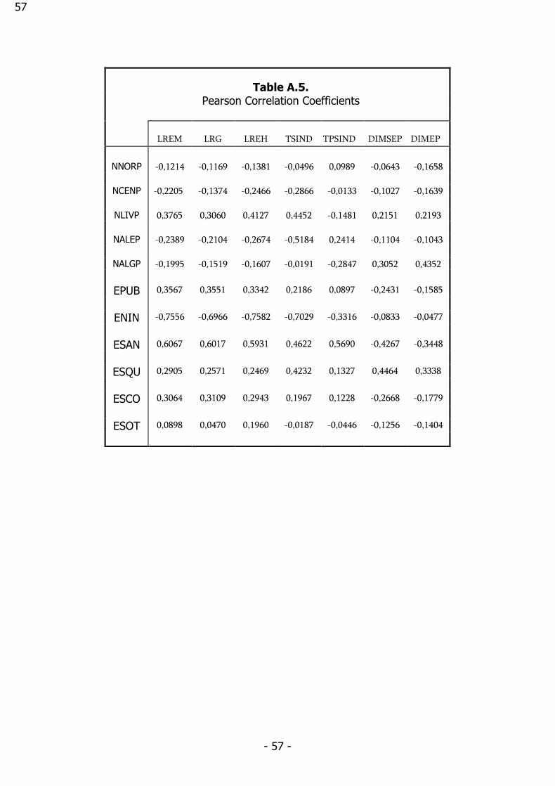
- 57 -

57

Table A.5. Pearson Correlation Coefficients

LREM LRG LREH TSIND TPSIND DIMSEP DIMEP

NNORP -0,1214 -0,1169 -0,1381 -0,0496 0,0989 -0,0643 -0,1658

NCENP -0,2205 -0,1374 -0,2466 -0,2866 -0,0133 -0,1027 -0,1639

NLIVP 0,3765 0,3060 0,4127 0,4452 -0,1481 0,2151 0,2193

NALEP -0,2389 -0,2104 -0,2674 -0,5184 0,2414 -0,1104 -0,1043

NALGP -0,1995 -0,1519 -0,1607 -0,0191 -0,2847 0,3052 0,4352

EPUB 0,3567 0,3551 0,3342 0,2186 0,0897 -0,2431 -0,1585

ENIN -0,7556 -0,6966 -0,7582 -0,7029 -0,3316 -0,0833 -0,0477

ESAN 0,6067 0,6017 0,5931 0,4622 0,5690 -0,4267 -0,3448

ESQU 0,2905 0,2571 0,2469 0,4232 0,1327 0,4464 0,3338

ESCO 0,3064 0,3109 0,2943 0,1967 0,1228 -0,2668 -0,1779

ESOT 0,0898 0,0470 0,1960 -0,0187 -0,0446 -0,1256 -0,1404

- 58 -

58

Table A.6. Pearson Correlation Coefficients

LREM LRG LREH TSIND TPSIND DIMSEP DIMEP

TSIND 0,5632 0,5216 0,5739 1 0,4006 0,0066 -0,0304

TPSIND 0,5087 0,5236 0,4770 0,4006 1 -0,4526 -0,5398

APT -0,4089 -0,4730 -0,4276 0,1283 -0,4696 0,1958 0,3527

APTE -0,2004 -0,2621 -0,2057 -0,0241 -0,5837 0,5116 0,8662

APNN* -0,4708 -0,4986 -0,4816 0,0502 -0,3893 0,3366 0,3705

DIMSEP -0,0172 -0,0029 -0,0333 0,0066 -0,4526 1 0,8263

DIMEP -0,0481 -0,0734 -0,0559 -0,0304 -0,5398 0,8263 1

DIMAP -0,0807 -0,0978 -0,0912 -0,0903 -0,6142 0,8744 0,9044

DIMSAP -0,4964 -0,4166 -0,5042 -0,3411 -0,0823 0,2896 0,0272

DIMCAP 0,3030 0,2935 0,3122 0,2430 0,2922 -0,0889 -0,1333

DIMPAP 0,3008 0,2889 0,3091 0,2533 0,2875 -0,0886 -0,1361

APAGP -0,1062 -0,0676 -0,1361 -0,2025 0,1138 0,1958 0,0264

APHIP 0,2617 0,2131 0,2927 0,3965 0,3380 -0,2080 -0,1213

APFMP 0,0388 0,0239 0,0093 0,1437 -0,2416 0,5233 0,5131

APPUP 0,1589 0,1111 0,1826 0,1749 -0,0582 0,1527 0,2646

APSEP 0,0813 0,0654 0,0872 0,2710 0,0522 0,2222 0,1559

APSCP -0,0934 -0,1106 -0,1213 0,0003 0,0301 0,1580 0,0594

APNNP -0,2694 -0,2695 -0,2445 -0,0143 -0,0478 0,5665 0,3424

DIMCAAP 0,3484 0,3532 0,3605 0,2099 0,5411 -0,3361 -0,2662

DIMPAAP 0,3560 0,3585 0,3679 0,2278 0,5505 -0,3415 -0,2718

APFMAP 0,1101 0,0832 0,1015 0,3630 0,1825 -0,0472 -0,0719

APSCAP 0,1120 0,1381 0,0915 -0,1668 0,5419 -0,4421 -0,3885

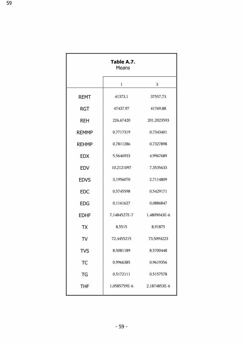
- 59 -

59

Table A.7. Means

1 3

REMT 41373,1 37557,73

RGT 47437,97 41769,88

REH 226,67420 201,2023593

REMMP 0,7717319 0,7343401

REHMP 0,7811286 0,7327898

EDX 5,5646933 4,9967689

EDV 10,2121097 7,3535633

EDVS 3,1956070 2,7114809

EDC 0,5745598 0,5429171

EDG 0,1161627 0,0886847

EDHF 7,1484527E-7 1,4809043E-6

TX 8,5515 8,91875

TV 72,4455215 73,5094223

TVS 8,5081189 8,5700448

TC 0,9966385 0,9619356

TG 0,5172111 0,5157578

THF 1,0585759E-6 2,1874853E-6

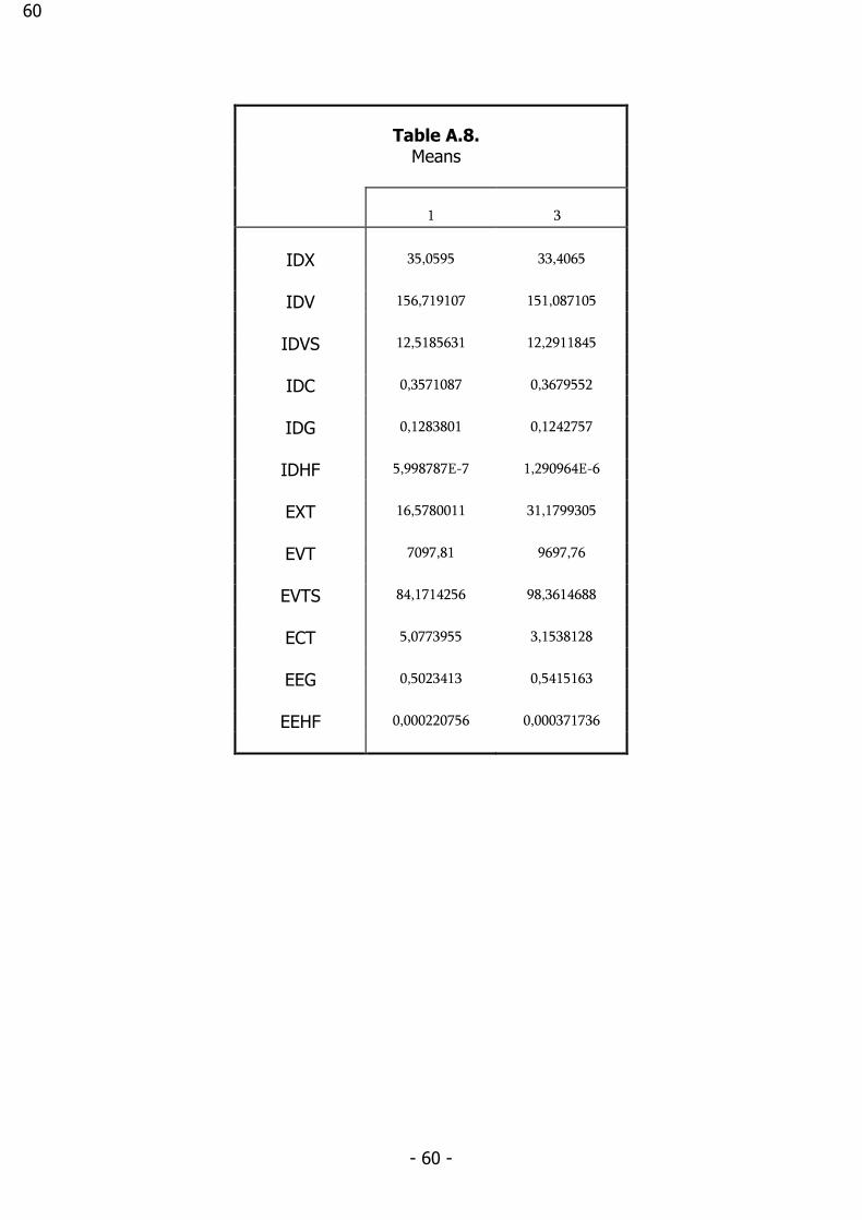
- 60 -

60

Table A.8. Means

1 3

IDX 35,0595 33,4065

IDV 156,719107 151,087105

IDVS 12,5185631 12,2911845

IDC 0,3571087 0,3679552

IDG 0,1283801 0,1242757

IDHF 5,998787E-7 1,290964E-6

EXT 16,5780011 31,1799305

EVT 7097,81 9697,76

EVTS 84,1714256 98,3614688

ECT 5,0773955 3,1538128

EEG 0,5023413 0,5415163

EEHF 0,000220756 0,000371736

- 61 -

61

Table A.9. Means

1 3

NXT 14,0083833 28,675945

NVT 2788,2 6875,56

NVTS 52,7446929 82,8426345

NCT 3,7637028 2,8881773

NNG 0,4210407 0,5087154

NNHF 0,000106377 0,000293329

TOP1 0,0199911 0,0127927

TOP2 0,0171188 0,0098842

TOP3 0,0384618 0,0378071

TOP4 0,0385605 0,0343524

TOP5 0,3885032 0,3742005

TOP6 0,1892038 0,2407125

TOP7 0,1145465 0,0785375

TOP8 0,1150138 0,1490596

TOP9 0,0786006 0,0626534

TOPM 0,3647638 0,4146985

- 62 -

62

Table A.10. Means

1 3

ACIP 0,0039153 0,0051884

ACIMP 0,000107736 0,000068792

ACIMM 0,0274414 0,0131445

TOTPI 1 0,4674989

HT 39,75 40,75

HET 4,5 4

HETP 0,000239359 0,000182748

HETPP 6,0195897E-6 4,4858617E-6

TDES 0,0474960 0,0561613

TD 0,0474830 0,0561340

TDES1 0,0534228 0,0629168

TDESM 0,0659291 0,0779898

TDM 0,0659087 0,0779397

TDESM1 0,0733225 0,0857410

- 63 -

63

Table A.11. Means

1 3

NNORP 0,390876 0,5148794

NCENP 0,144235 0,1698468

NLIVP 0,397709 0,2873343

NALEP 0,037394 0,0194626

NALGP 0,029787 0,0084769

EPUB 0,000519287 0,000522099

ENIN 0,3691618 0,3693525

ESAN 0,0172646 0,0252901

ESQU 0,5367550 0,5802960

ESCO 0,0125968 0,0076590

ESOT 0,0637026 0,0168803

- 64 -

64

Table A.12. Means

1 3

TSIND 52,6 72,8667

TPSIND 46,1 49,2025

APT 380,25 107,75

APTE 212920,5 18795,8

APNN* 1703,5 475

DIMSEP 1,74787 0,64093

DIMEP 55,54597 3,9666

DIMAP 559,727 174,6699

DIMSAP 0,0031287 0,0036509

DIMCAP 11166,5 14097,4

DIMPAP 12157,79 15463,35

APAGP 1,20127 1,38295

APHIP 0,216261 0,23806

APFMP 0,083548 0,05090

APPUP 1161 551,261

APSEP 1,599206 1,42496

APSCP 0,55818 0,67932

APNNP 4,47671 4,52381

DIMCAAP 19,86721 82,89484

DIMPAAP 21,63786 90,84574

APFMAP 0,0001489 0,00029

APSCAP 0,0009959 0,003944