Analysis of different numerical

procedures for determining the random

and chaotic earthquake properties

R. Magaña*, A. Hermosillo*, M. Pérez**

*Instituto de Ingeniería

Universidad Nacional Autónoma de México

Ciudad Universitaria, 04510 México, Distrito Federal

e-mail: rmat@pumas.iingen.unam.mx

** Centro Tecnológico Aragón

FES Aragón, UNAM

Email: marcelo@tigre.aragon.unam.mx

September 2010

Introduction• The purposes of this paper are:

• - To consider nonlinear dynamical aspects, in the criteria for structural and geotechnical design.

• - show that some earthquakes have chaotic content in addition to the random one. Taking into account that are non-stationary processes, so they must use appropriate mathematical tools (not limited to criteria used in stationary linear dynamic).

• Like examples of application of these concepts, the chaotic content analysis was realized for three earthquakes in Mexico, occurred in: Aguamilpa dam in Nayarit, Acapulco and Mexico City. The procedure followed is based on concepts of chaotic Hamiltonian mechanics, which is a generalization of the classic mechanics, and it lies on iterative equation systems, called maps.

• This article briefly discusses some of the mathematical models of nonlinear dynamic systems, and criteria for identifying the chaotic time series content as well as the application of these criteria to the earthquakes mentioned.

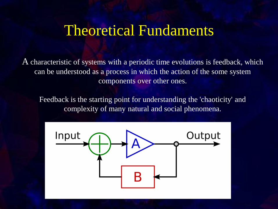
Theoretical Fundaments

A characteristic of systems with a periodic time evolutions is feedback, which

can be understood as a process in which the action of the some system

components over other ones.

Feedback is the starting point for understanding the 'chaoticity' and

complexity of many natural and social phenomena.

Solutions of differential equations in

phase space.

Hamiltonian dynamics. A wide class of

physical phenomena can be described by

Hamiltonian equations. This class includes

particles, fields, classical and quantum objects,

and it makes up a significant part of our

knowledge of the basics of dynamics in nature.

Hamiltonian dynamics is very different from,

for example, dissipative dynamics, and its

analysis uses specific tools that cannot be

applied in other cases. Discovery of chaotic

dynamics is a result of discovering new

features in Hamiltonian dynamics and new

types of solutions of the dynamical equations.

Hamiltonian equation

A Hamiltonian system with N degrees of freedom is characterized by a

generalized coordinate vector , generalized momentum vector , and a

Hamiltonian H = H(p, q) such that the equations of motion are:

i

ii

q

H

dt

dpp

i

i

ip

H

dt

dqq

Ni ,,1

The space (p, q) is 2N-dimensional phase space and a pair (pi, qi).

The Hamiltonian can depend explicitly on time, i.e. H = H(p, q t). Then the system

can be considered in an extended space of 2(N + 1) variables.

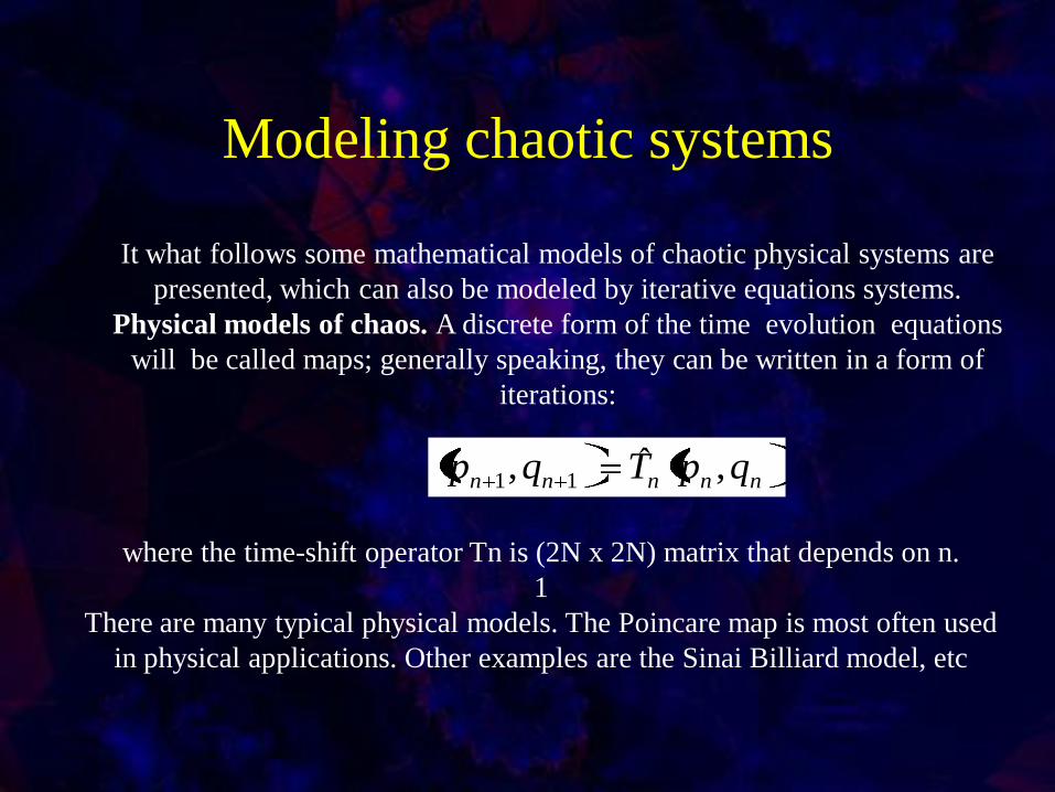
Modeling chaotic systems

It what follows some mathematical models of chaotic physical systems are

presented, which can also be modeled by iterative equations systems.

Physical models of chaos. A discrete form of the time evolution equations

will be called maps; generally speaking, they can be written in a form of

iterations:

nnnnn qpTqp ,ˆ, 11

where the time-shift operator Tn is (2N x 2N) matrix that depends on n.

1

There are many typical physical models. The Poincare map is most often used

in physical applications. Other examples are the Sinai Billiard model, etc

Universal and standard mapThe following is an example of a chaotic system which is a particular case of

Hamiltonian potential function, which includes shocks (given as a series of

pulses). Consider a Hamiltonian:

- T

t(x) fK + Ho(P) = H n

in which perturbation is a periodic sequence of δ function type pulses (kicks)

following with period T= 2π/v, K is an amplitude of the pulses, is a frequency

and (f(x)≤1) is some function. The equations of motion, corresponding to (2), are

- T

t(x)' fK - = p n p (P)H' = x 0

Tpxx nnn 11

There is a special case for and f(x) = -cos(x) and w(p) = p

Take into account the before we can derive the iteration equation:

nnn xKTfpp '1

For small K << 1 we can replace the difference equations with

the differential ones: This is the pendulum equation, and its

solutions are presented in figure 1.

Figure 1. Solution of pendulum equation in phase space

Fractals and chaos

Any kind of equation is an approximate way to describe an ensemble of

trajectories or particles, while neglecting some details of dynamics. All this

means that, depending upon the information about the system we would like

to preserve, the type and specific structure of the kinetic equation depends on

our choice of the reduced space of variables and on the level of coarse-

graining of trajectories. These properties of dynamics require a new approach

to kinetics (based on fractional differential equations) when the scaling

features of the dynamics dominate others and, moreover, do not have a

universal pattern as in the case of Gaussian processes, but instead, are

specified by the phase space topology and the corresponding characteristics of

singular zones.

Fractals and chaos

Structuring in the phase space. As has been noted, the solutions in the phase

space for chaotic systems give rise to specific structures, which are induced

by attractors, and are classified to classical and chaotic dynamics as follows.

Stable attractors (or classic dynamic). In the phase diagrams, these

converge on stable points, whereas in periodic signals, the trajectories have

well-defined paths.

Strange attractors (chaotic dynamics). These movements correspond to

unpredictable, irregular and seemingly random curves in the phase diagram,

but are located according to some probabilistic distribution within a certain

structure. A dynamical systems that converge in the long run to a strange

attractor is called chaotic.

Dynamical systems can be classified according to the behaviour of their orbits

(Espinosa, 2005). These orbits correspond to the movement in which the

system evolves over time. Thus, if the system moves in a set such that the set

of orbits A is a subset of , then the orbits will have the following behavior:

- Dissipative system: If A shrinks over time.

- System expansion: If A expands over time.

- System conservative: If A is maintained over time.

Typical chaotic oscillators

There are well-known chaotic oscillators, which

are characterized by iterative systems of equations,

due to space limitations in this study, only one is

discussed in what follows.

The changes over time of four well-known low-

dimensional chaotic systems are studied: Lorenz,

Rössler, Verhulst, and Duffing (Laurent et al.,

2010). Only the first is presented below. The

Lorenz system was designed for convection

analysis and is not generally used to study

population data.

Lorenz attractor standard values for the constants

were set as follows (through an iterative equation

system):

xyzz

xzyxy

yxx

3

8

28

2010

Detection AlgoritthmsThe possibility of reaching chaotic trajectories in nonlinear dynamical

systems leads naturally to the empirical question of how to distinguish such

trajectories of other really random time series (Gimeno et al., 2004). The topic

about the chaotic detection has attracted the attention of scientists from

different disciplines that have used different statistical procedures to measure

chaos.

In common usage, "chaos" means "a state of disorder", but the adjective

"chaotic" is defined more precisely in chaos theory (Wikipedia, 2010).

Although there is no an universally accepted mathematical definition of

chaos, a commonly-used definition says that, for a dynamical system to be

classified as chaotic, it must have the following properties:

• it must be sensitive to initial conditions,

• it must be topologically mixing, and

• its periodic orbits must be dense.

Detection Algoritthms

Sensitivity to initial conditions means that each point in such a system is

arbitrarily closely approximated by other points with significantly

different future trajectories. Thus, an arbitrarily small perturbation of the

current trajectory may lead to significantly different future behaviour.

Topological mixing (or topological transitivity) means that the system will

evolve over time so that any given region or open set of its phase space will

eventually overlap with any other given region. This mathematical concept of

"mixing" corresponds to the standard intuition, and the mixing of colored dyes

or fluids is an example of a chaotic system.

Density of periodic orbits means that every point in the space is approached

arbitrarily closely by periodic orbits. Topologically mixing systems failing

this condition may not display sensitivity to initial conditions, and hence may

not be chaotic.

There are different procedures to detect chaos, in what follows some of them

are commented.

Peters (Peters, 1994) tries to find evidence of a series with chaotic behaviour

by graphic analysis and notes that the series of financial asset prices have

graphically the same structure, whatever the timescale studied (Espinosa,

2005). The fact that these series have the same appearance on different time

scales is an indication that this is a fractal.

For the reconstruction of the recurrence maps is necessary to find hidden

patterns and structural changes in the data or similarities in patterns across the

time series under study. Thus, a signal off determinism will be when more

structured is the recurrence map. A random signal is when the recurrence

map is more uniform distributed on the phase space and does not have an

identifiable pattern.

Traditional methods of time series analysis come from the well-established

field of digital signal processing. Most traditional methods are well-

researched and their proper application is understood. One of the most

familiar and widely used tools is the Fourier transform. However, these

methods are designed to deal with a restricted subclass of possible data. The

data is often assumed to be stationary, that is, the dynamics generating the

data are independent of time. With experimental nonlinear data, traditional

signal processing methods may fail because the system dynamics are, at best,

complicated, and at worst, extremely noisy. In general, more advanced and

varied methods are often required.

Another tool for analyzing time series is the wavelet transform (WT). The WT

has been introduced and developed to study a large class of phenomena such

as image processing, data compression, chaos, fractals, etc. The basic

functions of the WT have the key property of localization in time (or space)

and in frequency, contrary to what happens with trigonometric functions. In

fact, the WT works as a mathematical microscope on a specific part of a

signal to extract local structures and singularities. This makes the wavelets

ideal for handling non-stationary and transient signals, as well as fractal-type

structures

Chaos indicatorsChaos indicators. Among these are: correlation

dimension, Lyapunov exponents, Kolmogorov

entropy, etc.

Correlation Dimension. A clear indicator that a

system is chaotic is to have a small correlation

dimension.

Lyapunov exponents. The most important indicator of

chaos in a nonlinear system is the Liapunov

exponents. They measured the speed at which a

system converges or diverges. They are calculated,

observation under observation, so a sample of size n

will have (n-1) exponents. The most important is the

greatest of them. If the greatest of all is negative, the

system will converge over time. However, if it is

positive, the error will grow exponentially over time,

and the system will exhibit the sensitive dependence

on initial conditions that are indicative of chaos.

The Lyapunov exponent characterises the extent of the sensitivity to initial

conditions (Wikipedia, 2010). Quantitatively, two trajectories in phase space

with initial separation diverge . where λ is the Lyapunov exponent. The rate

of separation can be different for different orientations of the initial separation

vector. Thus, there is a whole spectrum of Lyapunov exponents; the number

of them is equal to the number of dimensions of the phase space. It is common

to just refer to the largest one, i.e. to the Maximal Lyapunov exponent (MLE),

because it determines the overall predictability of the system. A positive MLE

is usually taken as an indication that the system is chaotic.

Kolmogorov entropy. The entropy of a dynamical system can be thought of as

the “disorder” to which the system tends with time. In this case the attractors,

if any, does not tend to disappear but to perpetuate itself, so the system is

chaotic. In terms of a decision rule can be concluded that a system is:

periodic if its entropy is close to 0%; Chaotic if it is between 0 and 100% and

Random if it is near of 100%.

The Hurst coefficient

The Hurst coefficient indicates the persistence or non-persistence in a time

series (Espinosa, 2005). Of being persistent, this would be a sign that this

series is not white noise and, therefore, there would be some kind of

dependency between the data.

The calculation of Hurst coefficient reveals that is given in the following

power law shown in equation (6):

HNa

NS

R

where a is a constant; N is the number of observations; H is the Hurst

exponent, is the statistic depends on the size series and is defined as the

coefficient of variation of the series divided by its standard deviation. The

Hurst coefficient is used to detect long-term memory in time series.

To calculate the correlation dimension Grassberger and Procaccia

(Grassberger et al, 1983) developed an efficient algorithm that suggest that ,

where D is the capacity dimension. The idea is to replace the algorithm to

calculate , called box-counting, by the estimation of distances between points

(which representing positions of the system along an orbit) in the attractor

set.

Developed software examples

Between that is an algorithm developed by Wolf (Wolf et al, 1985), which

implements the theory in a very simple and direct fashion (Kodba et al.,

2004). The whole program package that can be downloaded from our Web

page (User) consists of five programs (embedd.exe, mutual.exe, fnn.exe,

determinism.exe and lyapmax.exe) and an input file ini.dat, which contains

the studied time series. All programs have a graphical interface and display

results in the forms of graphs and drawings.

For these reasons the Nonlinear Dynamics Toolbox was created (Reiss, 2001).

The Nonlinear Dynamics Toolbox (NDT) is a set of routines for the creation,

manipulation, analysis, and display of large multi-dimensional time series

data sets, using both established and original techniques derived primarily

from the field of nonlinear dynamics. In addition, some traditional signal

processing methods are also available in NDT.

Chaotic Analysis of Earthquakes

A common methodology used to determinate if a system have chaotic

behavior is the next: firstly, it is used the embedding delay of coordinates in

order to reconstruct the attractor system of the time series analyzed (phase

space); for this purpose, both, the embedding delay (t) and embedding

dimension (m) have to be calculated. Two methods are used: the mutual

information method to estimate the appropriate embedding delay and the false

nearest neighbor method (FNN) to estimate the embedding dimension. Next, a

determinism test is performed to determine if the series were obtained of

chaotic or random systems. Finally, the computation of the maximal

Lyapunov exponent is performed to determinate if chaos in the phenomenon

is present

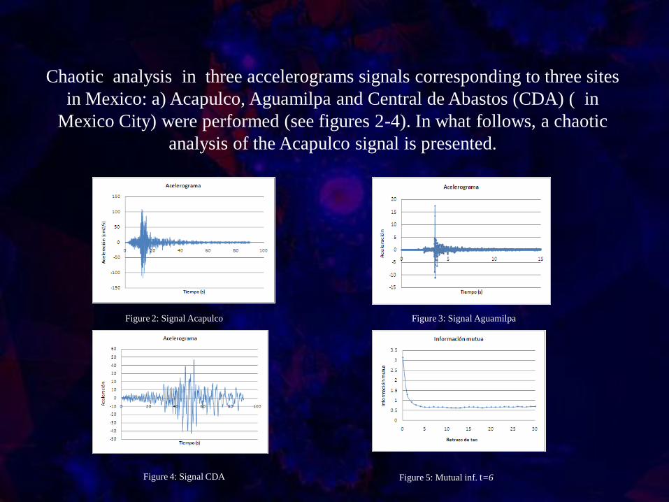
Figure 2: Signal Acapulco Figure 3: Signal Aguamilpa

Figure 4: Signal CDA Figure 5: Mutual inf. t=6

Chaotic analysis in three accelerograms signals corresponding to three sites

in Mexico: a) Acapulco, Aguamilpa and Central de Abastos (CDA) ( in

Mexico City) were performed (see figures 2-4). In what follows, a chaotic

analysis of the Acapulco signal is presented.

Chaotic analysis software

The software used to calculate the parameters m and t, the phase space

reconstruction, the determinism test and the estimation of the maximal

Lyapunov exponent can be consult and download from the site on the

web (user).

Phase space reconstruction

Below, the estimation of the parameters m and t which are necessary for the

phase space reconstruction using the mutual information and the FNN

methods is presented (see figures 5 and 6).

In the figure 7 a projection in a plane of the attractor system is presented.

Figure 8 shows the graph corresponding to the determinism (determ)

test and finally, in figure 9, the estimation of the maximal Lyapunov

exponent is presented.

Figure 6: FNN. m=4 Figure 7: Phase space

Figure 8. Determ =0.638 Figure 9. Maximal Lyapunov exponent=0.9

Table 1. Resume of results

Signal

m Determ Max Exp

Lyap

Acapulco 6 4 0.638 0.90

Aguamilpa 1 5 0.397 0.68

CDA 10 10 0.723 0.60

From the analysis presented it can be concluded that the three signals have a chaotic behavior.

In table 1 a resume of the analysis made to the three signals is presented.

Conclutions

1. There are different classes of systems: mechanical, electronic,

biological, economic, etc., represented by systems of differential

equations of integer and fractional order, which can be replaced by

iterative equations systems, and have movement histories which

when are to be represented in a phase diagram have complex

topological structures (including fractal type).

2. There are several algorithmic procedures by which they can analyze

time series and deduce whether these come from deterministic

chaotic systems or are either purely random kind.

3. To consider the cases of nonlinear dynamics is important because

usually the design procedures are based on linear dynamic

mathematical models or purely random, but this strategy is not

entirely appropriate because most natural processes are not

stationary, like earthquakes, and therefore it is necessary to develop

a more consistent design methodology.

Conclutions

4. From the analysis presented, it can be concluded that the analyzed

signals were generated from a deterministic chaotic phenomenon

because the vector field turned out to be deterministic and the

maximal Lyapunov exponent was positive, suggesting that the

reconstructed system have an important deterministic chaotic

component.

5. The fact that the earthquakes have chaotic content, reveals clearly that

the signals detected in each place, have effects of the geologic

system where were registered.