analysis of microsoft, google and apple stock prices

ANALYSIS OF MICROSOFT, GOOGLE AND

APPLE STOCK PRICES

JUSTIN RODRIGUES

HIRA NADEEM

INTRODUCTION

Stock market is an important part of the economy. The stock market plays a pivotal role in the

growth of the industry and commerce of the country that eventually affects the economy of the country to a

great extent. That is reason that the government, industry and even the central banks of the country keep a close

watch on the happenings of the stock market. This is the primary function of the stock exchange and thus they

play the most important role of supporting the growth of the industry and commerce in the country. That is the

reason that a rising stock market is the sign of a developing industrial sector and a growing economy of the

country. Investors buy stocks with the belief that the company will grow continuously to raise the value of their

shares. Acquiring stocks from a new company is considered to be more risky than buying shares from a well-

established company but the potential gain is much greater.

For the purpose of our study, we wish to analyze the stock market for three of the leading companies in

the technical world, MICROSOFT, GOOGLE AND APPLE and then determine their success rates based on the

models that these companies follow. The data is taken from Yahoo finance which provides information for over

9000 companies, including contact information, business summaries, officer and employee information, sector

and industry classifications, business and earnings announcement summaries, and financial statistics and ratios.

The stock data for each company ranges from January 1, 2008 to March 31, 2012. Overall, that makes 1071

observations. Since stocks are not traded over weekends or on holidays, only on so-called trading days, the

stock values do not change over weekends or holidays. For simplicity, we will analyze the data as if they were

equally spaced. Overall, we wish to study the reasons for the rise and fall in the stock price of the three

companies during a certain amount of time. Further, we want to see if all these companies follow the same or

different time series models and if, possible, we will try to predict the future stock growth. Our main goal would

be to come up with a model using various techniques that may fit our data for each of the three companies like

ARIMA, ACF/PACF, normality tests, residue analysis, as well as some of the financial models like ARCH and

GARCH.

STATISTICAL ANALYSIS

For the initial research into the topic, we analyzed some time series plots for the three companies.

The time series plot for all of the three companies show that they might follow the same model,

though there is more increase in the stock price of apple as compared to the price of stocks for Microsoft and

Google.

Looking at the trend, we can see an overall increase in the stock price in the stocks of these three

companies with a huge dip that started in October, 2008 when the stock market crashed. Low interest rates

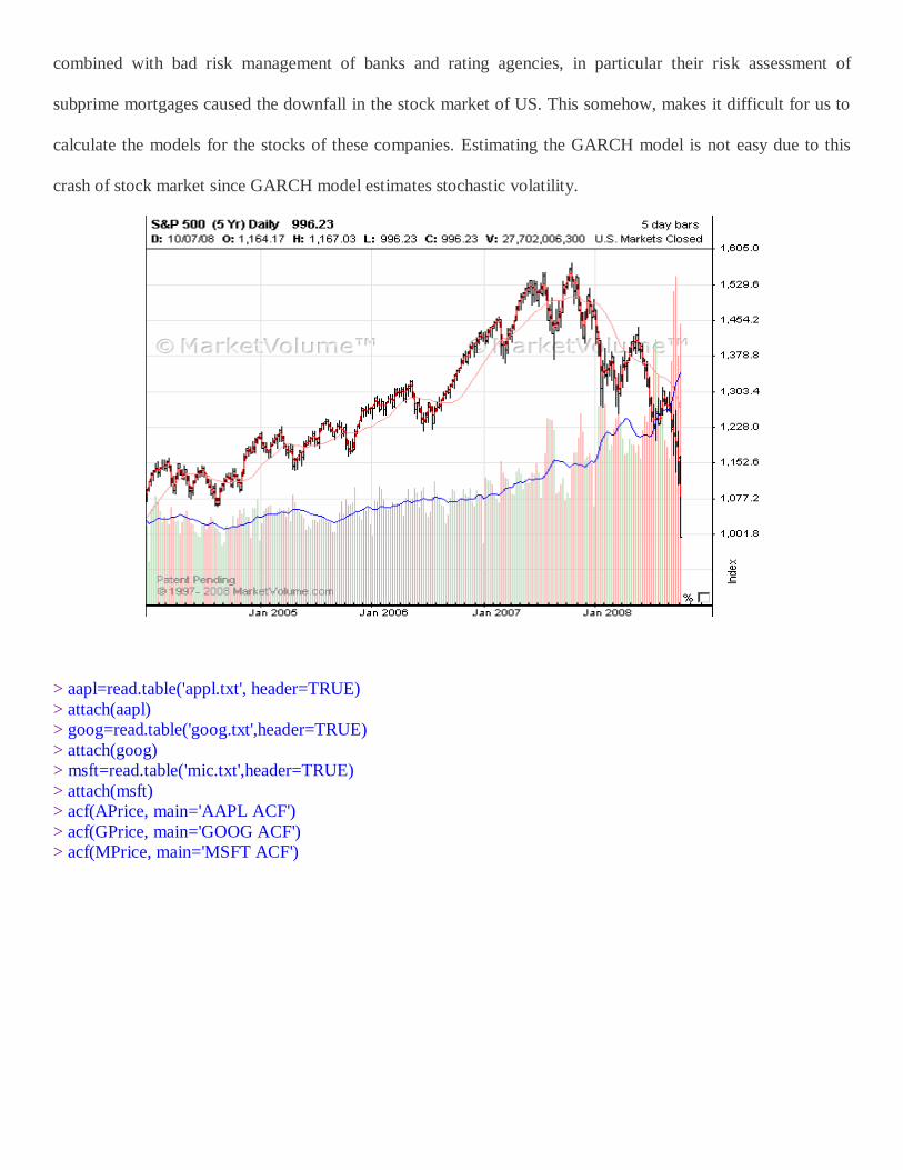
combined with bad risk management of banks and rating agencies, in particular their risk assessment of

subprime mortgages caused the downfall in the stock market of US. This somehow, makes it difficult for us to

calculate the models for the stocks of these companies. Estimating the GARCH model is not easy due to this

crash of stock market since GARCH model estimates stochastic volatility.

> aapl=read.table('appl.txt', header=TRUE)

> attach(aapl)

> goog=read.table('goog.txt',header=TRUE)

> attach(goog)

> msft=read.table('mic.txt',header=TRUE)

> attach(msft)

> acf(APrice, main='AAPL ACF')

> acf(GPrice, main='GOOG ACF')

> acf(MPrice, main='MSFT ACF')

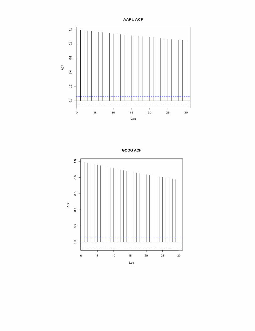
All the autocorrelation functions for three companies show an exponential decay, and thus, by Box-Jenkins

Approach there is no evidence for the presence of Moving Average.

> pacf(APrice, main='AAPL PACF')

> pacf(GPrice, main='GOOG PACF')

> pacf(MPrice, main='MSFT PACF')

Using the partial autocorrelation functions, we can see that apart from lag 1, there are no other

significant lags, and hence, by Box-Jenkins Approach, there is no evidence for the presence for the

Autoregressive model. So, ARMA fail to be the model for any of the three stock prices.

Using the regression model approach, lm() we obtained the following data.

Apple

> model1=lm(APrice~time(APrice))

> summary(model1)

Coefficients:

Estimate Std. Error t value Pr(>|t|)

(Intercept) 61.415658 2.946335 20.84 <2e-16 ***

time(APrice) 0.340697 0.004762 71.55 <2e-16 ***

Plotting an abline of model1 to the Apple Stock price plot shows us that our data is not linear, as this does not

produce a good enough fit for our model. The R-squared value is 0.827, which shows that at least 82.7% of the

model is captured by this linear model, but the plot shows otherwise.

> plot(APrice,type='l',ylab='Stock Price', main="AAPL", xlab='Time')

> abline(model1)

Google

> model2=lm(GPrice~time(GPrice))

> summary(model2)

Coefficients:


(Intercept) 4.210e+02 4.741e+00 88.79 <2e-16 ***

time(APrice) 1.640e-01 7.662e-03 21.40 <2e-16 ***

Plotting a linear trend model for Google Stock does not produce an accurate trend either as we can see below.

For Google’s price, our linear modeling produced an Adjusted R-Squared of 0.2993, which means that the data

is not captured well by this linear approximation at all.

> plot(GPrice,type='l',ylab='Stock Price', main="GOOG", xlab='Time')

> abline(model2)

Microsoft

> model3=lm(MPrice~time(MPrice))

> summary(model3)

Coefficients:


(Intercept) 2.489e+01 2.181e-01 114.126 < 2e-16 ***

time(MPrice) 2.014e-03 3.524e-04 5.715 1.42e-08 ***

Following the same procedure as with AAPL and GOOG, we see that MSFT is an even poorer fit than the other

two in terms of linear modeling. The Adjusted R-Square of 0.2874 confirms what we can observe visually from

the plot below, that this data is not linear in nature.

Modelling

Our next goal is to determine which model our data follows. Clearly our raw stock price data did not

follow any clearly visible trend. Our next option was to take the logged difference of each of the stocks prices

in order to consider the daily growth rate of each stock’s price, with the hope of being left with white noise data

after the transformation. Logging converts absolute differences into relative (i.e., percentage) differences. Thus,

the series DIFF(LOG(Y)) represents the percentage change in Y from period to period. The input series need to

be stationary, i-e it should have a constant mean, variance and autocorrelation function with time. Log

transforming the data stabilizes the data.

Apple

> ALD=diff(log(APrice))

> plot.ts(ALD, main="diff(log(AAPL))", ylab='Growth Rate', xlab='Time')

> abline(h=0)

The diff(log(y)) series of Apple is not stationary since it varies more in the beginning and in the end,

it shows a bit increasing trend. So, the series is not stationary.

Next we examined the ACF and PACF for the logged and differenced data for Apple, here referred to as ALD.

(Apple Logged and Differenced)

> par(mfrow=c(2,1))

> acf(ALD)

> acf(ALD, type='partial')

The autocorrelation and partial autocorrelation functions of logarithm differenced series represents

that it is not an ARIMA model since using the Box-Jenkins Approach no lags in the ACF is significant, i-e

different from zero, so there is no evidence for Moving Average Model, similarly, using PACF, we can say

none of the lags are significant, so there is no evidence of Autoregressive Model. Thus, overall, log(diff(y))

model is not an ARIMA model.

Google

> GLD=diff(log(GPrice))

> plot.ts(GLD, main="diff(log(GOOG))", ylab='Growth Rate', xlab='Time')

> abline(h=0)

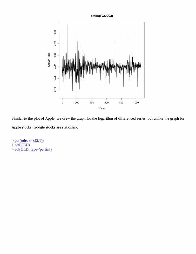
Similar to the plot of Apple, we drew the graph for the logarithm of differenced series, but unlike the graph for

Apple stocks, Google stocks are stationary.

> par(mfrow=c(2,1))

> acf(GLD)

> acf(GLD, type='partial')

Even though the diff(log(GOOG)) is stationary, there is no evidence of ARIMA model. Using Box-

Jenkins Approach, none of the lags in the autocorrelation and partial autocorrelation functions are significant, so

there is no evidence of Moving Average in ACF and Autoregressive Model in PACF. So, overall, there is no

ARIMA model for the Google Stock Price.

Microsoft

> MLD=diff(log(MPrice))

> plot.ts(MLD, main="diff(log(MSFT))", ylab='Growth Rate', xlab='Time')

> abline(h=0)

The differenced logarithm series for Microsoft Stock Price is stationary with mean zero. So, there

might be a presence of ARIMA model.

> par(mfrow=c(2,1))

> acf(MLD)

> acf(MLD,type='partial')

Similar to the differenced logarithm series of Google, there is no evidence of the presence of

ARIMA model, using the Box-Jenkins Approach, since none of the lags are significantly different from zero, so

there is no ARIMA model.

We next took the logged and differenced data for all three stocks, and examined the distribution of each stock’s

return.

APPLE

An excellent test of normality is known as the Shapiro-Wilk test. It essentially calculates the

correlation between the residuals and the corresponding normal quantiles. The lower this correlation, the more

evidence we have against normality.

Looking at the Shapiro-Wilkes test of normality we see that this data is not normally distributed.

> shapiro.test(rAAPL)

Shapiro-Wilk normality test

data: rAAPL

W = 0.9405, p-value < 2.2e-16

GOOGLE

> shapiro.test(rGOOG)


data: rGOOG

W = 0.902, p-value < 2.2e-16

Applying this test to these residuals gives a test statistic of W = 0.902 with a very small p-value of

2.2e-16. The test shows that Google stock market for the logged differenced series is not normal. The graph is

thick-tailed from the ends.

MICROSOFT

> shapiro.test(rMSFT)


data: rMSFT

W = 0.9188, p-value < 2.2e-16

Applying this test to these residuals gives a test statistic of W = 0.9188 with a very small p-value of

2.2e-16. The test shows that Microsoft stock market for the logged differenced series is not normal. The graph

is thick-tailed from the ends.

Thus, the stock prices of all the three companies are not normal.

The thickness of the tail of a distribution relative to that of a normal distribution is often measured by

the (excess) kurtosis. For normal distributions, the kurtosis is always equal to zero. A distribution with positive

kurtosis is called a heavy-tailed distribution, whereas it is called light-tailed if its kurtosis is negative.

> kurtosis(rAAPL)

[1] 6.694315

> kurtosis(rGOOG)

[1] 8.315009

> kurtosis(rMSFT)

[1] 7.579608

All of the three stock price logged differenced series have a positive kurtosis representing that all of these series

are heavy-tailed.

Skewness is a measure of the asymmetry of the probability distribution of a real-valued random

variable. The skewness value can be positive or negative, or even undefined. Qualitatively, a negative skew

indicates that the tail on the left side of the probability density function is longer than the right side and the bulk

of the values (possibly including the median) lie to the right of the mean. A positive skew indicates that

the tail on the right side is longer than the left side and the bulk of the values lie to the left of the mean. A zero

value indicates that the values are relatively evenly distributed on both sides of the mean, typically but not

necessarily implying a symmetric distribution.

> skewness(rAAPL)

[1] -0.5528693

> skewness(rGOOG)

[1] 0.4376514

> skewness(rMSFT)

[1] 0.2844724

By the value of skewness, rAAPL is negatively skewed indicating that the tail on the left side is

longer on the right side, and most values lie on the right side, whereas the positive values of skewness for

Google returns and Microsoft returns indicates the tail on the right side is longer than the left side and bulk of

values lie to the left of mean.

Since none of our data suggested an ARIMA model, it was time to explore the possibility that these

stock prices had a heteroscedastic property where their variance changed with time. Modelling

heteroskedasticity, i.e. time- or state-dependent conditional variance in linear

regression models, is an important problem to which a number of solutions has been

proposed in the time series literature ranging from an ad-hoc Box-Cox transformation

over generalized least-squares methods to the Generalized AutoRegressive Conditional

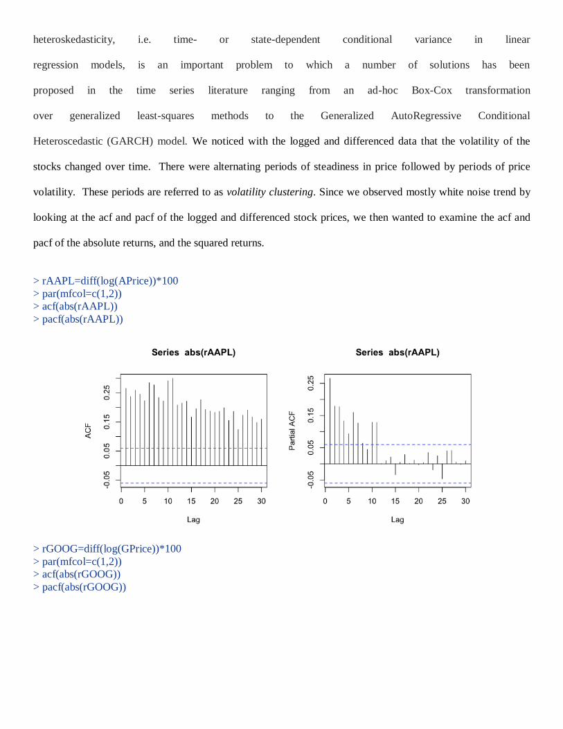
Heteroscedastic (GARCH) model. We noticed with the logged and differenced data that the volatility of the

stocks changed over time. There were alternating periods of steadiness in price followed by periods of price

volatility. These periods are referred to as volatility clustering. Since we observed mostly white noise trend by

looking at the acf and pacf of the logged and differenced stock prices, we then wanted to examine the acf and

pacf of the absolute returns, and the squared returns.

> rAAPL=diff(log(APrice))*100

> par(mfcol=c(1,2))

> acf(abs(rAAPL))

> pacf(abs(rAAPL))

> rGOOG=diff(log(GPrice))*100

> par(mfcol=c(1,2))

> acf(abs(rGOOG))

> pacf(abs(rGOOG))

> rMSFT=diff(log(MPrice))*100

> par(mfcol=c(1,2))

> acf(abs(rMSFT))

> pacf(abs(rMSFT))

Next we examined the squared returns and their acf/pacf for each of the three companies. The squared returns

provide an unbiased estimator. A series with large squared returns may foretell a relatively volatile period.

Conversely, a series of small squared returns may foretell a relatively quiet period.

Now, we need to distinguish between series values being uncorrelated and series values being independent. If

series values are truly independent, then nonlinear instantaneous transformations such as taking logarithms,

absolute values, or squaring preserves independence.

> par(mfcol=c(1,2))

> acf(rAAPL^2)

> pacf(rAAPL^2)

> par(mfcol=c(1,2))

> acf(rGOOG^2)

> pacf(rGOOG^2)

> par(mfcol=c(1,2))

> acf(rMSFT^2)

> pacf(rMSFT^2)

Now, we want to see if the model representing the stock market of these three companies is ARCH, so

we use the McLeod Li Test. In practice, it is useful to apply the McLeod-Li test for ARCH using a number of

lags and plot the p-values of the test.

>McLeod.Li.test(y=rAAPL, main='McLeod Li Test for rAAPL')

The McLeod test indicates that there is no evidence of the ARCH model for the returns of Apple stock price.

>McLeod.Li.test(y=rGOOG, main='McLeod Li Test for rGOOG')

The McLeod Li Test for the return of Google Stock Price indicates a presence of either ARCH or GARCH

model.

> McLeod.Li.test(y=rMSFT, main='McLeod Li Test for rMSFT')

From the McLeod Test we can see that only Google’s stock price appears to be a proper candidate for

ARCH/GARCH modeling.

To identify the order of a mixed model, we use the extended autocorrelation function (EACF)

First we looked at the EACF for return data for Google. Which suggested a GARCH(1,1) or possibly

GARCH(2,2) model.

> eacf(rGOOG)

AR/MA

0 1 2 3 4 5 6 7 8 9 10 11 12 13

0 o o o o o o o x o o o x o o

1 x o o o o o o x x o o x o o

2 x x o o o o o x x o o o o o

3 x x x o o o o x o o o o o o

4 x x o o o o o x o o o o o o

5 x x x o o o o o o o o o o o

6 x x o o o o o o o o o o o o

7 x x x x o x x o o o o o o o

In order for us to analyze and interpret which model would be the best selection for GOOG, we needed to check

whether or not each model’s assumptions were supported by our data. We did this by inspecting the

standardized residuals from different fitted GARCH(p,q) models of daily Google returns. The model that

produces standardized residuals that appear to be most indepently and identically distributed will be our correct

choice.

> m1=garch(x=rGOOG, order=c(1,1))




> par(mfcol=c(2,2))

> plot(residuals(m1),type='h', main='GARCH(1,1)',ylab='Standardized Residuals')




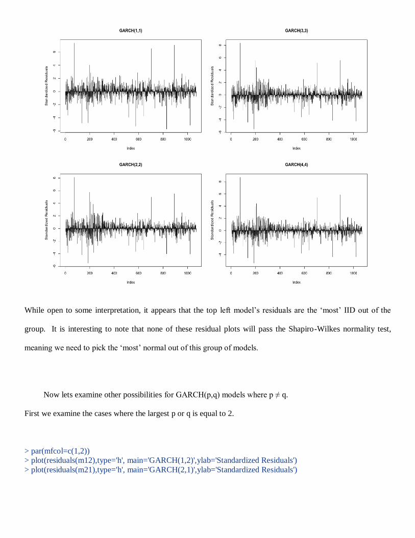
While open to some interpretation, it appears that the top left model’s residuals are the ‘most’ IID out of the

group. It is interesting to note that none of these residual plots will pass the Shapiro-Wilkes normality test,

meaning we need to pick the ‘most’ normal out of this group of models.

Now lets examine other possibilities for GARCH(p,q) models where p ≠ q.

First we examine the cases where the largest p or q is equal to 2.

> par(mfcol=c(1,2))



Then we examided the models with the largest p or q is equal to 3.

> par(mfcol=c(1,2))



Finally we examined the possible GARCH(p,q) models where the highest value of p or q is 4.

> par(mfcol=c(3,2))







We opted to stop after evaluating the first 16 possible models, as we saw very little improvement in

the residuals’ normality. We then took the 4 most independent and identically distributed looking of these 16

plots and applied portmanteau tests to further determine which residuals are the most normalized, thereby

hopefully identifying the best model for Google’s stock price.

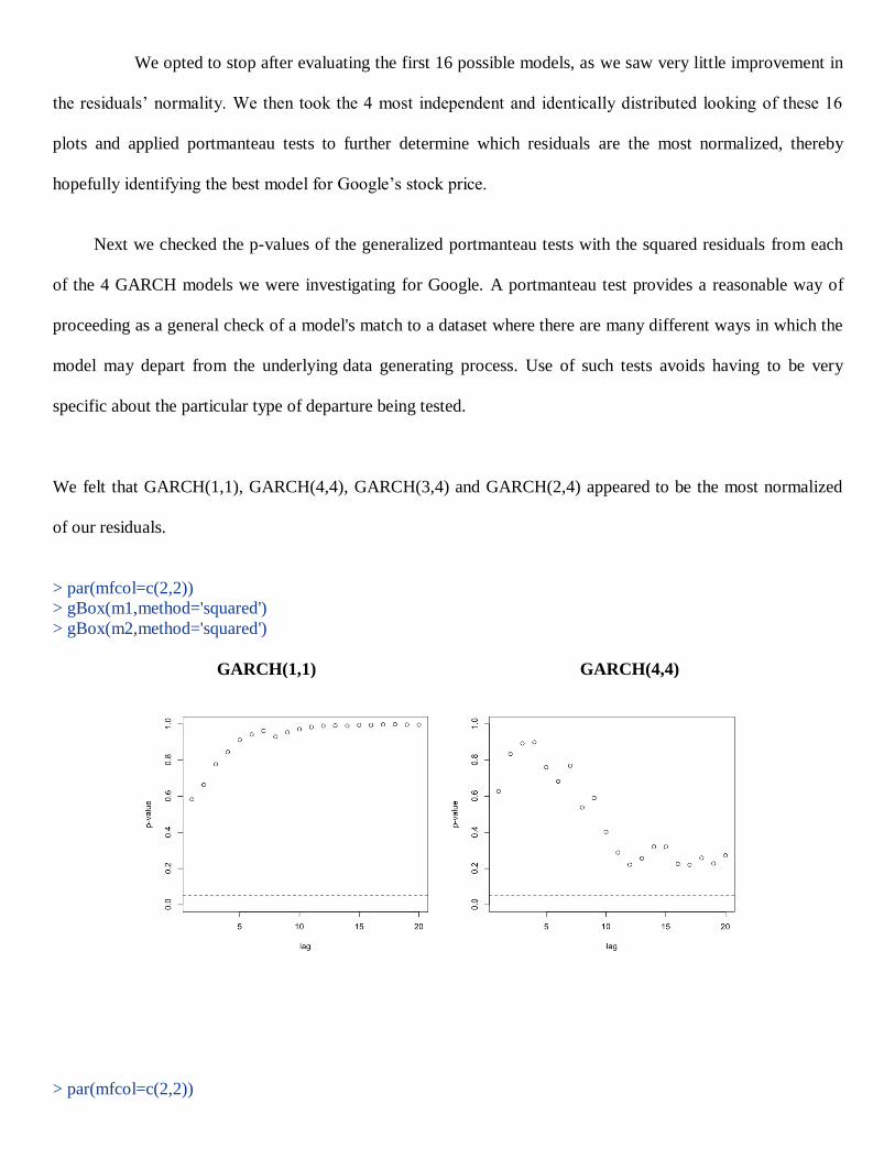
Next we checked the p-values of the generalized portmanteau tests with the squared residuals from each

of the 4 GARCH models we were investigating for Google. A portmanteau test provides a reasonable way of

proceeding as a general check of a model's match to a dataset where there are many different ways in which the

model may depart from the underlying data generating process. Use of such tests avoids having to be very

specific about the particular type of departure being tested.

We felt that GARCH(1,1), GARCH(4,4), GARCH(3,4) and GARCH(2,4) appeared to be the most normalized

of our residuals.

> par(mfcol=c(2,2))

> gBox(m1,method='squared')


GARCH(1,1) GARCH(4,4)

> par(mfcol=c(2,2))



GARCH(3,4) GARCH(2,4)

It is clear that the model with the highest p-values is GARCH(1,1). From this we concluded that the best

GARCH(p,q) model would be GARCH(1,1).

Forecasting of the GARCH model is difficult.

CONCLUSION

Analysis of the Stock Market is not an easy job. Unexpected fluctuations in the market make the study and

prediction of the Stock Market difficult and vague. We attempted to study the pattern of the stock prices of the

three leading technology companies; Apple, Microsoft and Google, and see if any model fits the stock prices

data from January, 2008 till March, 2012. Time Series plots of each of these showed fluctuations throughout

with Apple having an overall increasing trend. However, when using the ACF or PACF plot, we showed that

there is no evidence of either an AR or MA model. Further, we take the logarithm difference of the series next.

Ploting the log(diff(y)) for the three series give us a stationary plot for Google and Microsoft and an increasing

trend for Apple. We then plotted the ACF and PACF for the difference series shows no lag is significance, so

there is no evidence for ARIMA Model. Then we check for the normality of the three diff(log(y)) series using

Shapiro-Wilk test, kurtosis and skewness. All of these show that all three series are not normal. Further, then we

look for the presence of ARCH or GARCH Model using the McLeod Test, so only Google shows some

evidence for ARCH or GARCH Model. We, then tested different GARCH(p,q) Model, first in case, where p=q

and second, in which p≠q for p,q ≤ 4. Thus, as a result of plotting these Models, we got GARCH(1,1) as best

Model for Google Stock Prices.

analysis of microsoft, google and apple stock prices

Documents