analytical formulae for the kirchhoff–routh path function in multiply...

Analytical formulae for the Kirchhoff–Routhpath function in multiply connected domains

BY DARREN CROWDY AND JONATHAN MARSHALL

Department of Mathematics, Imperial College of Science,Technology and Medicine, 180 Queen’s Gate, London SW7 2AZ, UK

([email protected]; [email protected])

Explicit formulae for the Kirchhoff–Routh path functions (or Hamiltonians) governingthe motion of N-point vortices in multiply connected domains are derived when allcirculations around the holes in the domain are zero. The method uses the Schottky–Klein prime function to find representations of the hydrodynamic Green’s function inmultiply connected circular domains. The Green’s function is then used to construct theassociated Kirchhoff–Routh path function. The path function in more general multiplyconnected domains then follows from a transformation property of the path functionunder conformal mapping of the canonical circular domains. Illustrative examples arepresented for the case of single vortex motion in multiply connected domains.

Keywords: point vortex; Kirchhoff–Routh; Hamiltonian

RecAcc

1. Introduction

The study of point vortex dynamics is an important area of fluid dynamicsalready commanding a vast literature. The review by Aref et al. (2002) providesa recent survey of results involving vortex equilibria (or vortex crystals), mainlyin unbounded and periodic configurations, while the recent monograph byNewton (2002) gives a broader perspective of the general N-vortex problem,including discussions of vortex motion in unbounded and bounded planardomains, as well as on curved surfaces such as the surface of a sphere.

Although the motion of point vortices in unbounded domains has receivedmuch attention, the theory of point vortex motion in domains bounded byimpenetrable walls is much less developed. The simplest example is a single-pointvortex adjacent to an infinite straight wall. Such a vortex translates at constantspeed, maintaining a constant distance from the wall. This motion isconveniently understood as being induced by an opposite circulation ‘image’vortex behind the wall. This is perhaps the simplest example of the celebrated‘method of images’ (Milne-Thomson 1968). Several more elaborate examplesinvolving simply connected fluid regions are given in ch. 3 of Newton (2002)while others are described by Saffman (1992). Many of these examples rely on thetransformation properties, under conformal mapping, of what is known as theKirchhoff–Routh path function, which is essentially the Hamiltonian governingthe vortex motion. The Hamiltonian formulation of point vortex dynamics and

Proc. R. Soc. A (2005) 461, 2477–2501

doi:10.1098/rspa.2005.1492

Published online 23 June 2005

eived 6 September 2004epted 4 April 2005 2477 q 2005 The Royal Society

D. Crowdy and J. Marshall2478

the Kirchhoff–Routh path function date back to the work of Kirchhoff & Routh(Routh 1881). It was reappraised much later by Lin (1941a,b), who consideredmultiply connected domains, and more recently by Flucher & Gustafsson (1997)(see also ch. 15 of Flucher 1999), who have analysed various aspects of thegeneral boundary-value problem arising from the problem of point vortex motionin bounded domains.

The motion of a single vortex in bounded, simply connected domains isrelatively well studied. Gustafsson (1979) and Richardson (1980) have shownthat the Kirchhoff–Routh path function satisfies an elliptic Liouville equation inthe bounded domain D and is infinite everywhere on the boundary. On thesubject of N-vortex motion in multiply connected domains, the literature issparse. Lin (1941a) established the existence and uniqueness of a generalizedKirchhoff–Routh path function in this case, but does not construct it explicitly orgive any specific examples.

In this paper, an analytical formula for the hydrodynamic Green’s functionintroduced by Lin (1941a) is found in the class of multiply connected circulardomains. This is achieved using a special transcendental function called theSchottky–Klein prime function (Baker 1995). A circular domain is a planardomain all of whose boundary components are circles. By using this Green’sfunction, formulae for the associated Kirchhoff–Routh path function for generalN-vortex motion in such circular domains can be constructed. However, Lin(1941b) has also shown how to derive formulae for the Kirchhoff–Routh pathfunction in conformally equivalent, multiply connected domains. Thus, if aformula for the conformal mapping from a given circular multiply connecteddomain to a more general domain is known, then the path function in the newdomain can be constructed in an analytical form.

2. The hydrodynamic Green’s function

Lin (1941a) introduced a special Green’s function G(x, y; x0, y0) with respect tothe two points (x, y) and (x0, y0) in a fluid domain D in the following way. Threeseparate cases of domain D (cases 1–3 below) are considered depending onwhether D is bounded or unbounded. Let MR0 be an integer. Suppose D isbounded by MC1 impenetrable walls, and let these boundaries of D befCj jjZ0; 1;.;Mg. If D is bounded, then C0 will be taken as the outer boundarywith fCk jkZ1;.;Mg denoting the M enclosed boundaries. If D is unboundedbut has a boundary extending to infinity, then this infinite-length boundarywill be denoted C0. Lin’s special hydrodynamic Green’s function is the functionG(x, y; x0, y0) satisfying the following properties.

(i)

Proc.

The function

gðx; y; x0; y0ÞZKGðx; y; x0; y0ÞK1

2plog r0; (2.1)

is harmonic with respect to (x, y) throughout the region D including at the

R. Soc. A (2005)

2479Formulae for the Kirchhoff–Routh path function

Proc.

point (x0, y0). Here, r0 is

r0 ZffiffiffiffiffiffiffiffiffiffiffiffiffiffiffiffiffiffiffiffiffiffiffiffiffiffiffiffiffiffiffiffiffiffiffiffiffiffiffiffiffiffiffiðxKx0Þ2CðyKy0Þ2

q: (2.2)

(ii)
If vG/vn is the normal derivative of G on a curve, then
Gðx; y; x0; y0ÞZAk; on Ck; k Z 1;.;M ;

#Ck

vG

vndsZ 0; k Z 1;.;M ;

9>=>; (2.3)

where ds denotes an element of arc and fAk jkZ1;.;Mg are constants.
(iii) Case 1. If D has a closed outer boundary C0, then
Gðx; y; x0; y0ÞZ 0 on C0: (2.4)

Case 2. If D is unbounded and extends to infinity in all directions, then over
(iv) a very large circle of radius r0, G behaves as follows:
Gðx; y; x0; y0ÞZK1

2plog r0 COð1=r0Þ;

vG

vsZOð1=r20 Þ;

vG

vnZK

1

2pr0COð1=r20 Þ;

9>>>>>>>=>>>>>>>;

(2.5)

where vG/vs is the tangential derivative along the circle.
(v) Case 3. If D is unbounded but has boundaries extending to infinity, then G
behaves as follows:

Gðx; y; x0; y0ÞZ 0; on C0;

Gðx; y; x0; y0ÞZ oð1Þ; on a very large circle of radius r0:

)(2.6)

n also established the following two lemmas.
Li
Lemma 2.1. The function G(x, y; x0, y0) defined by conditions (i)–(v) aboveexists uniquely and is a generalized Green’s function satisfying the reciprocitycondition

Gðx; y; x0; y0ÞZGðx0; y0; x; yÞ: (2.7)

Lemma 2.2. If N vortices of strengths fGk j kZ1;.;Ng are present inan incompressible fluid at the points {(xk, yk)jkZ1,.,N } in a generalregion D bounded by fixed boundaries, the streamfunction of the fluid motion isgiven by

jðx; y; x1; y1;.; xN ; yN ÞZj0ðx; yÞCXNkZ1

GkGðx; y; xk; ykÞ; (2.8)

where the properties of G are given in lemma 2.1 and j0(x, y) is thestreamfunction due to outside agencies and satisfying the boundary conditions

R. Soc. A (2005)


of no flow through the domain boundaries. j0 is independent of the point vortexpositions.

Finally, Lin establishes the following theorem.

Theorem 2.3. For the motion of vortices of circulations fGk jkZ1;.;Ng in ageneral region D bounded by fixed boundaries, there exists a Kirchhoff–Routhfunction H(x1, y1,., xN, yN) such that

Gk

dxkdt

ZvH

vyk; Gk

dykdt

ZKvH

vxk; (2.9)

where H(x1, y1,., xN, yN) is given by

Hðx1;y1;.;xN ;yN ÞZXNkZ1

Gkj0ðxk;ykÞCXN

k1;k2Z1

k1Ok2

Gk1Gk2Gðxk1 ;yk1 ;xk2 ;yk2Þ

K1

2

XNkZ1

G2kgðxk ;yk;xk ;ykÞ: ð2:10Þ

In rescaled coordinates ðffiffiffiffiffiGk

pxk ;

ffiffiffiffiffiGk

pykÞ equation (2.9) is a Hamiltonian system

in canonical form.Flucher & Gustafsson (1997) refer to Lin’s special Green’s function as the

hydrodynamic Green’s function and we will adopt this terminology. They alsoconsider an associated function called the Robin function. It is the regular part ofthe above hydrodynamic Green’s function evaluated at the singularity. If thehydrodynamic Green’s function G is decomposed into a radially symmetricsingular part and a regular part as in equation (2.1), then the Robin functionR(x0, y0) is defined as

Rðx0; y0Þhgðx0; y0; x0; y0Þ: (2.11)

This implies that, near the singularity at (x0, y0), G can be expanded as

Gðx; y; x0; y0ÞZK1

2plog r0 KRðx0; y0ÞCOðr0Þ: (2.12)

It is more convenient for what follows to introduce complex coordinates zZxCiyand �zZxK iy. Thus, if the complex number aZx0Ciy0 denotes the complexposition of the singularity of the Green’s function we will henceforth writeG(z; a) instead of G(x, y; x0, y0).

3. Construction of G in circular domains

We will now show how to construct an explicit representation for G in a general,multiply connected circular domain of arbitrary finite connectivity. Let Dz bethe interior of the unit z-disc with M smaller circular discs excised. MZ0 is thesimply connected case. Let the boundaries of these smaller circular discs bedenoted fCj jjZ1;.;Mg. Let the unit circle jzjZ1 be denoted C0. The complex

Proc. R. Soc. A (2005)


numbers fdj jjZ1;.;Mg are the centres of the enclosed circular discs while thereal numbers fqj jjZ1;.;Mg will denote their radii.

This special class of multiply connected domains is significant for two reasons.First, such circular domains are known to be canonical domains for conformalmapping to general multiply connected domains (Nehari 1952). That is, anygiven multiply connected domain can be obtained by conformal mapping of acircular domain of the same connectivity for some choice of the parametersfdj jjZ1;.;Mg and fqj jjZ1;.;Mg. These parameters must be determined aspart of the construction of the conformal mapping and, in the latter context, arereferred to as the conformal moduli of the domain (Nehari 1952). Second, Lin(1941b) gives explicit formulae for the transformation properties of theKirchhoff–Routh path function under conformal mapping. In particular, ifa conformal map z(z) maps a given region Dz in a z-plane to a region Dz in a

z-plane, and H (z) and H (z), respectively, denote the Hamiltonians in the z andz-planes, then these Hamiltonians are related by the formula

H ðzÞðz1; �z1;.; zN ; �zN ÞZH ðzÞðz1; �z1;.; zN ; �zN ÞCXNkZ1

G2k

4plogjzzðzkÞj; (3.1)

where fzk jkZ1;.;Ng and fzkZzðzkÞjkZ1;.;Ng are the point vortexpositions in the z- and z-planes, respectively.

In combination, these two facts mean that the formulae to be derived in thispaper will theoretically yield formulae for the Kirchhoff–Routh path function forN vortices in any multiply connected domain for which a conformal mappingfrom a circular preimage region is known explicitly.

4. Schottky groups

First, define M Mobius maps ffj jjZ1;.;Mg corresponding to the conjugationmap for points on the circle Cj. That is, if Cj has equation

jzKdj j2 Z ðzKdjÞð�zK�djÞZ q2j ; (4.1)

then

�zZ �dj Cq2j

zKdj; (4.2)

and so

fjðzÞh�dj Cq2j

zKdj: (4.3)

If z is a point on Cj , then its complex conjugate is given by �zZfjðzÞ.Next, introduce the Mobius maps

qjðzÞh �fjðzK1ÞZ dj Cq2j z

1K�djz: (4.4)

Let C 0j be the circle obtained by reflection of the circle Cj in the unit circle jzjZ1

(i.e. the circle obtained by the transformation z11=�z). It is easily verified thatthe image of the circle C 0

j under the transformation qj is the circle Cj . Since the M


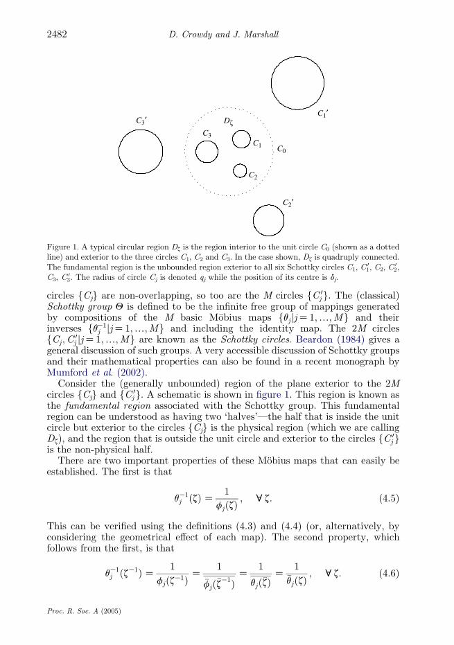
Figure 1. A typical circular region Dz is the region interior to the unit circle C0 (shown as a dottedline) and exterior to the three circles C1, C2 and C3. In the case shown, Dz is quadruply connected.The fundamental region is the unbounded region exterior to all six Schottky circles C1, C

01, C2, C

02,

C3, C03. The radius of circle Cj is denoted qj while the position of its centre is dj.


circles {Cj} are non-overlapping, so too are the M circles fC 0j g. The (classical)

Schottky group Q is defined to be the infinite free group of mappings generatedby compositions of the M basic Mobius maps fqj jjZ1;.;Mg and theirinverses fqK1

j jjZ1;.;Mg and including the identity map. The 2M circlesfCj ;C

0j jjZ1;.;Mg are known as the Schottky circles. Beardon (1984) gives a

general discussion of such groups. A very accessible discussion of Schottky groupsand their mathematical properties can also be found in a recent monograph byMumford et al. (2002).

Consider the (generally unbounded) region of the plane exterior to the 2Mcircles {Cj} and fC 0

j g. A schematic is shown in figure 1. This region is known asthe fundamental region associated with the Schottky group. This fundamentalregion can be understood as having two ‘halves’—the half that is inside the unitcircle but exterior to the circles {Cj} is the physical region (which we are callingDz), and the region that is outside the unit circle and exterior to the circles fC 0

j gis the non-physical half.

There are two important properties of these Mobius maps that can easily beestablished. The first is that

qK1j ðzÞZ 1

fjðzÞ; cz: (4.5)

This can be verified using the definitions (4.3) and (4.4) (or, alternatively, byconsidering the geometrical effect of each map). The second property, whichfollows from the first, is that

qK1j ðzK1ÞZ 1

fjðzK1ÞZ

1

�fjð�zK1Þ

Z1

qjð�zÞZ

1�qjðzÞ

; cz: (4.6)



Some special infinite subsets of mappings in a given Schottky group will beneeded in what follows. A special notation is now introduced. This notation is notstandard but is introduced here to clarify the presentation.

The full Schottky group is denoted Q. The notation iQj is used to denote allmappings in the full group, which do not have a power of qi or q

K1i on the left-hand

end or a power of qj or qK1j on the right-hand end. As a special case of this, the

notationQj simplymeans allmappings in the group that do not have any positive ornegative power of qj at the right-hand end (but with no stipulation about whatappears on the left-hand end). Similarly, jQ means all mappings that do not haveany positive or negative power of qj at the left-hand end (but with no stipulationabout what appears on the right-hand end). In addition, the single prime notationwill be used to denote a subset where the identity is excluded from the set; thus,Q0

1denotes allmappings, excluding the identity and all transformationswith a positiveor negative power of q1 at the right-hand end. The double prime notation will beused to denote a subset where the identity and all inverse mappings are excludedfrom the set. This means, for example, that if q1q2 is included in the set, thenthe mapping qK1

2 qK11 must be excluded. Thus, Q 00 means all mappings excluding

the identity and all inverses. Similarly, the notation 1Q002 denotes all mappings,

excluding inverses and the identity, which do not have any power of q1 or qK11 on

the left-hand end or any power of q2 or qK12 on the right-hand end. Likewise, Q00

j

denotes allmappings, excluding the identity and all inverses, which do not have anypositive or negative power of qj at the right-hand end.

5. The Schottky–Klein prime function

Following Baker (1995), the Schottky–Klein prime function is defined as

uðz;gÞZ ðzKgÞu0ðz;gÞ; (5.1)

where the function u 0(z, g) is given by

u0ðz;gÞZYqi2Q00

ðqiðzÞKgÞðqiðgÞKzÞðqiðzÞKzÞðqiðgÞKgÞ ; (5.2)

and where the product is over all mappings qi in the set Q00; u0 can also bewritten as

u0ðz;gÞZYqi2Q00

fz; qiðzÞ;g; qiðgÞg; (5.3)

where the brace notation denotes a cross-ratio of the four arguments. This will beuseful later. The function u(z, g) is single valued on the whole z-plane and has azero at g and all points equivalent to g under the mappings of the group Q. Theprime notation is not used here to denote differentiation.

The Schottky–Klein prime function has some important transformationproperties. One such property is that it is antisymmetric in its arguments,that is,

uðz;gÞZKuðg; zÞ: (5.4)



This is clear from inspection of equations (5.1) and (5.2). A second importantproperty is given by

uðqjðzÞ;g1ÞuðqjðzÞ;g2Þ

Z bjðg1;g2Þuðz;g1Þuðz;g2Þ

; (5.5)

where qj is any one of the basic maps of the Schottky group. A detailed derivationof this result is given in ch. 12 of Baker (1995). A formula for bj(g1, g2) is

bjðg1;g2ÞZYqk2Qj

ðg1 KqkðBjÞÞðg2KqkðAjÞÞðg1 KqkðAjÞÞðg2KqkðBjÞÞ

; (5.6)

where Aj and Bj are the two fixed points of the mapping qj satisfying

qjðAjÞZAj ; qjðBjÞZBj : (5.7)

Aj and Bj satisfy an equation of the form

qjðzÞKBj

qjðzÞKAj

Zmj eikj

zKBj

zKAj

; (5.8)

for some real constants mj , kj , and are distinguished by the fact that jmjj!1 inequation (5.8). For the distribution of Schottky circles fCj ;C

0j g considered in §4,

the prime function also has the property that

�uðzK1;gK1ÞZK1

zguðz;gÞ; (5.9)

where the conjugate function �uðz;gÞ is defined by

�uðz;gÞZuð�z; �gÞ: (5.10)

A derivation of equation (5.9) is given in appendix A.It is convenient to categorize all possible compositions of the basic maps

according to their level. As an illustration, consider the case in which there arefour basic maps fqj jjZ1; 2; 3; 4g. The identity map is considered to be the level-zero map. The four basic maps, together with their inverses, fqK1

j jjZ1; 2; 3; 4gconstitute the eight level-one maps. All possible combinations of any two of theseeight level-one maps which do not reduce to the identity, for example,

q1ðq1ðzÞÞ; q1ðq2ðzÞÞ; q1ðq3ðzÞÞ; q1ðq4ðzÞÞ; q2ðq1ðzÞÞ; q2ðq2ðzÞÞ;.;

(5.11)

will be called the level-two maps; all possible combinations of any three ofthe eight level-one maps that do not reduce to a lower-level map will be calledthe level-three maps, and so on.

On a practical note, to write a function routine to calculate u(z,g)numerically, it is necessary to truncate the infinite product in equation (5.1).This is achieved in a natural way by including all Mobius maps up to somechosen level and truncating the contribution to the product from all higher-levelmaps. The truncation, which includes all maps up to level three, has been used tocompute the examples in this paper. The software programme MATLAB is



particularly suited to construction of the Schottky–Klein prime function becausethe action of an element of the Schottky group on the point z can be written asmultiplication by a 2!2 matrix on the vector (z, 1)T—a linear algebra operationthat is performed very efficiently in MATLAB.

6. Explicit solution for G

Given a circular domain Dz with given moduli (such as that shown in figure 1),the associated Schottky–Klein prime function u(z, g) can be constructed. Let thesingularity of the hydrodynamic Green’s function G in this domain be at a. Thecomplex potential W(z; a) for the flow is such that

Gðz;aÞZ Im½W ðz;aÞ�; (6.1)

and an explicit expression for it is

W ðz;aÞZKi

4plog

uðz;aÞ�uðzK1;aK1Þuðz; �aK1Þ�uðzK1; �aÞ

� �: (6.2)

It is natural to choose the branch of the logarithm so that the branch points at aand �aK1 are joined by a branch cut, as are all image-pairs of these two pointsunder the transformations of the group (i.e. in all regions ‘equivalent’ to thefundamental region). An explicit representation for G(z;a) is

Gðz;aÞZ Im½W ðz;aÞ�ZK1

4plog


��: (6.3)

Formulae (6.2) and (6.3) are the principal new results of this paper.In order to prove that equations (6.2) and (6.3) satisfy the conditions outlined

above, consider the function

Sðz;aÞhuðz;aÞ�uðzK1;aK1Þuðz; �aK1Þ�uðzK1; �aÞ

: (6.4)

S(z;a) has a second-order zero at zZa (as well as at all points in the planeequivalent to a under the action of the group). S(z;a) also has a second-orderpole at the point �aK1 (and all equivalent points). Let a be a point in the physicalhalf of the fundamental region. It follows that �aK1 will be in the non-physicalhalf. Since

Gðz;aÞZK1

4plogjSðz;aÞj; (6.5)

this means that, in the physical half of the fundamental region Dz, G(z;a) has asingle isolated logarithmic singularity at zZa, as required. Given that the zero ofS at a is second order, locally, G(z;a) has the expansion

Gðz;aÞZK1

2plogjzKajCOð1Þ; (6.6)

again as required.



It has yet to be verified that equation (6.3) satisfies the required boundaryconditions on all the circles fCj jjZ0; 1;.;Mg. On C0,

Sðz;aÞ Z �uðzK1; �aÞuðz; �aK1Þ�uðzK1;aK1Þuðz;aÞ

Z1

Sðz;aÞ ; (6.7)

where we have used the fact that �zZzK1 on C0. Since jS(z;a)jZ1 on C0, then itfollows from equation (6.5) that

Gðz;aÞZ 0; on C0: (6.8)

This is the normalization condition stipulated in equation (2.4).On the other hand, on any one of the interior circles fCj jjZ1;.;Mg,

Sðz;aÞ Z�uðfjðzÞ; �aÞuðfjðzÞK1; �aK1Þ�uðfjðzÞ;aK1ÞuðfjðzÞK1;aÞ

Z�uð�qjðzK1Þ; �aÞuð�qjðzK1ÞK1; �aK1Þ�uð�qjðzK1Þ;aK1Þuð�qjðzK1ÞK1;aÞ

Z�uð�qjðzK1Þ; �aÞ�uð�qjðzK1Þ; �aÞ

jaj2 �uð�qjðzK1Þ;aK1Þ�uð�qjðzK1Þ;aK1Þ:

(6.9)

However, we can now use equation (5.5) to give

Sðz;aÞ Zbjða; �aK1Þ2 �uðzK1; �aÞ�uðzK1; �aÞjaj2 �uðzK1;aK1Þ�uðzK1;aK1Þ

Zbjða; �aK1Þ2 uðz; �aK1Þ�uðzK1; �aÞ

uðz;aÞ�uðzK1;aK1ÞZ

bjða; �aK1Þ2

Sðz;aÞ :

(6.10)

Formula (6.10) immediately implies that, on Cj ,

jSðz;aÞjZ bjða; �aK1Þ; (6.11)so that

Gðz;aÞZK1

4plogjSðz;aÞjZK

1

4plog bjða; �aK1Þ; on Cj : (6.12)

This means the parameters fAj jjZ1;.;Mg of equation (2.3) are

Aj ZK1

4plog bjða; �aK1Þ: (6.13)

Utilizing equation (5.6), a formula for bjða; �aK1Þ is

bjða; �aK1ÞZYqk2Qj

ðaKqkðBjÞÞð�aK1KqkðAjÞÞðaKqkðAjÞÞð�aK1 KqkðBjÞÞ

: (6.14)

From equation (6.10), bjða; �aK1Þ must be a real quantity, but it is not clear frominspection whether the right-hand side of equation (6.14) is always real. Forcompleteness, a demonstration of this is given in appendix B. It turns out that forany a2C, fbjða; �aK1Þg are all real positive quantities. Finally, some algebraic



manipulations reveal that the associated Robin function is given by

Rða; �aÞZ 1

4plog

u0ða;aÞ�u0ðaK1;aK1Þa2uða; �aK1Þ�uðaK1; �aÞ

��: (6.15)

(a ) Normalization and symmetry

Lemma 2.1 states that the hydrodynamic Green’s function satisfies areciprocity relation given by

Gðz;aÞZGða; zÞ: (6.16)

It is appropriate to verify that the explicit formula given in equation (6.3)satisfies equation (6.16) because it is not obvious by inspection. To this end,consider

Gða; zÞZK1

4plog

uða; zÞ�uðaK1; zK1Þuða; �zK1Þ�uðaK1; �zÞ

��: (6.17)

Note first that, by using equation (5.4),

juða; zÞ�uðaK1; zK1ÞjZ juðz;aÞ�uðzK1;aK1Þj: (6.18)

Next, note that

juða; �zK1ÞjZ j�uð�a; zK1ÞjZ j�uðzK1; �aÞj; (6.19)

where the first equality is simply a statement of the fact that the moduli ofcomplex conjugate numbers are equal and the second equality follows from theuse of equation (5.4). By similar manipulations

j�uðaK1; �zÞjZ juð�aK1; zÞjZ juðz; �aK1Þj: (6.20)

By using equations (6.18)–(6.20) in equation (6.17), the reciprocity relation(6.16) is confirmed.

Utilizing equation (5.9), it is also possible to write W(z; a), and hence G(z; a),in the alternative equivalent forms

W ðz;aÞZKi

2plog

1

jajuðz;aÞuðz; �aK1Þ

� �; Gðz;aÞZK

1

2plog

1

a

uðz;aÞuðz; �aK1Þ

��: (6.21)

However, we prefer the representations given in equations (6.2) and (6.3),because it is easily seen from these formulae that the normalization GZ0 on C0

has been enforced. This normalization is crucial not only for the uniqueness of thehydrodynamic Green’s function, but also so that the reciprocity condition (6.16)is satisfied (Flucher & Gustafsson 1997).

(b ) Conditions on R on the boundaries

A result given in Flucher & Gustafsson (1997) is that the Robin functionRða; �aÞ is singular on all boundaries of the domain. It is appropriate to verify this



for the Robin function (6.15) found for the case of multiply connected circulardomains.

First, note that as a tends to a point on C0, it is clear that because a and �aK1

have the same argument, they will approach each other as jaj/1. Thus, thedenominator in the argument of the logarithm in equation (6.15) will tend to zeroin this limit. This verifies that Rða; �aÞ is singular on C0.

Similarly, for a point a on fCj jjZ1;.;Mg, note that

juða; �aK1ÞjZ juðfjðaÞ; �aK1ÞjZ juðfj ð�aÞ; �aK1ÞjZ juðqjð�aK1Þ; �aK1Þj: (6.22)

However, this final term is zero using the fact that uðz; �aK1Þ has a zero at �aK1 andat all transformations of this point under the mappings of the group Q. Inparticular, it will have a zero at qjð�aK1Þ. Given that juða; �aK1Þj appears as thedenominator of the argument of the logarithm in equation (6.15), and becausethe numerator is easily seen not to vanish, it follows that Rða; �aÞ is singular at allpoints on the boundaries fCj jjZ1;.;Mg.

(c ) Round-island circulations

The circulation around the j th island is by definition

Re

�#Cj

dW

dzdz

�ZRe

�#Cj

dW

�ZRe½W �Cj

; (6.23)

where the notation ½W �Cjdenotes the change in value of W on making a

single circuit around the closed curve Cj . By the choice of logarithmic branchcuts in the z-plane made earlier, none of the branch cuts across any of thecircles fCj jjZ1;.;Mg; hence W does not change value on making a circuit ofany of these circles. The round-island circulations are therefore all zero.However, the same is not true of the unit circle C0, because a branch cut crossesC0 in order to join a to �aK1. If it is also required to render the circulation aroundC0 equal to zero (case 2 of the definition in §2), then another point vortex ofopposite circulation KG must be added in the physical half of the fundamentalregion. Let this additional vortex be at a point b. The complex potential for avortex of circulation G will then become

W ðz;a; bÞZKiG

4plog


� �

CiG

4plog

uðz; bÞ�uðzK1; bK1Þuðz; �bK1Þ�uðzK1; �bÞ

!;

(6.24)

where the branch of the function is chosen so that branch cuts join a to b insidethe physical half of the fundamental region, while another branch cut joins �aK1 to�bK1

in the non-physical half (with analogous choices of cuts being made in allother equivalent regions). This construction is particularly useful in the case ofunbounded flows, where C0 is conformally mapped to an (MC1)th island andthere is a point zN in Dz mapping to infinity. If it is required to make thecirculation around this island zero (so that all round-island circulations are zero),



then it is usual to add an additional point vortex of circulation KG to the pointat infinity, with b being taken to be zN. In their studies of vortex motion pasttwo circular islands, Johnson & McDonald (2004a) also introduce a point vortexsingularity at infinity to render the circulation around both islands equal to zero.

(d ) Inter-island fluxes

It is well known that the difference between two values of G evaluated on twodifferent islands gives the (time-dependent) ‘inter-island flux’ of fluid between thetwo islands. Let Fij denote the flux between islands i and j, then by usingequation (6.12), we can obtain explicit formulae for the values of these fluxes. Inparticular,

Fij ZK1

4plog

bið�a;aK1Þbjð�a;aK1Þ

� �; (6.25)

where the explicit formula (6.14) can be used.

7. The Kirchhoff–Routh path function

Using the representations for the hydrodynamic Green’s and Robin functions incircular domains derived in §6, it is now possible to write down formulae for theKirchhoff–Routh path function as given in equation (2.10) for any finite numberN of vortices in a multiply connected circular region. However, our result isstronger than this once we exploit the second result (3.1) from Lin (1941b)showing how the Hamiltonian transforms under conformal mapping.

We summarize our results in a more explicit statement of theorem 2.3.

Theorem 7.1. For the motion of vortices of strengths fGkjkZ1;.;Ng in ageneral region Dz bounded by fixed boundaries, first construct the Kirchhoff–Routh path function H ðzÞða1; �a1;.;aN ; �aN Þ in a conformally equivalent circularregion Dz of the form

H ðzÞða1; �a1;.;aN ; �aN Þ

ZXNkZ1

Gkj0ðakÞCXNk1;k2Z1

k1Ok2

Gk1Gk2Gðak1 ;ak2ÞK1

2

XNkZ1

G2kRðak ; �akÞ;

(7.1)

where G(z; a) is given in equation (6.3), Rða; �aÞ is given in equation (6.15) andj0(z) is the contribution to the Hamiltonian from external agencies such asbackground flows or non-zero round-island circulations. Then, if z(z) is theconformal map from Dz to Dz, the Kirchhoff–Routh path function for the N-vortexmotion is

H ðzÞðz1; �z1;.; zN ; �zN ÞZH ðzÞða1; �a1;.;aN ; �aN ÞCXNkZ1

G2k

4plogjzzðakÞj; (7.2)

where zkZz(ak) for kZ1,.,N.



In cases where both j0(z) and the conformal mapping z(z) are knownexplicitly, it follows that the Hamiltonian will also be given in analytical form byusing equation (7.2). Even when either of the functions j0(z) and z(z) is notknown analytically (and must be computed numerically), these two functions areindependent of the instantaneous point vortex positions, and can be computed atthe start of any calculation (assuming the boundaries of the flow domain and theflow due to external agencies are not changing in time). In any case, theHamiltonian given in equation (7.2) can still facilitate numerical calculation ofeven very complicated N-vortex flows.

8. The single vortex case

To illustrate the usefulness of the formulae derived in this paper, we include someexamples for the motion of a single vortex. This also provides us the opportunityto examine how our general formulation reduces to the simply and doublyconnected studies that have already appeared in the literature.

First, we write down the Hamiltonians for single-vortex flow in the three typesof domain (cases 1–3) considered in §2.

Case 1. When just a single vortex is present, the double sum in equation (2.10)disappears and the Kirchhoff–Routh path function, in the absence of externalsources of vorticity, for a circulation-G point vortex reduces to

H ðzÞða; �aÞZKG2

2Rða; �aÞ: (8.1)

By using equation (6.15), this becomes

H ðzÞða; �aÞZKG2

8plog

u0ða;aÞ�u0ðaK1;aK1Þa2uða; �aK1Þ�uðaK1; �aÞ

��: (8.2)

Let z(z) be any map from the circular domain to a (conformally equivalent)multiply connected domain. Then, by equation (3.1), the Hamiltonian in thez-plane is given by

H ðzÞðza; �zaÞZH ðzÞða; �aÞC G2

4plogjzzðaÞj; (8.3)

where zaZz(a). Equivalently,

H ðzÞðza; �zaÞZKG2

8plog

1

a2

u0ða;aÞ�u0ðaK1;aK1Þuða; �aK1Þ�uðaK1; �aÞ

1

zzðaÞ2

��: (8.4)

If the conformal map z(z) is known explicitly, then equation (8.4) gives theHamiltonian in explicit form.

Case 2. In the case where D is unbounded but has a single boundary thatextends to infinity, C0 is taken to map to the infinite boundary (so that theGreen’s function is zero on this boundary as required in the definition given in§2), and the Hamiltonian is again given by equation (8.4).

Case 3. In the case where D is unbounded in all directions, it is necessary toadd a point vortex at infinity with circulation KG in order to render zero the



circulation around all islands. Let zN be the point in Dz mapping to physicalinfinity. Then, the complex potential for the point vortex at infinity is

WNðzÞZiG

4plog

uðz; zNÞ�uðzK1; zK1N Þ

uðz; �zK1N Þ�uðzK1; �zNÞ

!; (8.5)

and the Hamiltonian equation (8.4) must be modified by the addition of

HNða; �aÞZG Im½WNðaÞ�; (8.6)

thereby yielding

H ðzÞðza; �zaÞZKG2

8plog

1

a2

u0ða;aÞ�u0ðaK1;aK1Þu2ða; �zK1N Þ�u2ðaK1; �zNÞ

uða; �aK1Þ�uðaK1; �aÞu2ða; zNÞ�u2ðaK1; zK1N Þ

1

zzðaÞ2

��:

(8.7)

In the case of a single vortex, the Hamiltonian H ðzÞðza; �zaÞ is a conserved quantityand the trajectories of the vortex are simply its level lines.

(a ) The simply connected case

Consider a simply connected domain. In this case, the Schottky group is thetrivial group and the associated Schottky–Klein prime function is just

uðz;gÞZ ðzKgÞ: (8.8)

The hydrodynamic Green’s function in a bounded domain reduces to

Gðz;aÞZK1

4plog

ðzKaÞðzK1KaK1ÞðzK �aK1ÞðzK1K �aÞ

��ZK

1

2plog

1

a

ðzKaÞðzK �aK1Þ

��

ZK1

2plogjzKajK 1

2plog

1

a

1

ðzK �aK1Þ

��:

(8.9)

The Robin function is

Rða; �aÞZ 1

2plog

1

1Ka�a

��: (8.10)

The Hamiltonian for a single vortex in a domain mapping from the unit z-circlevia a mapping z(z) (with the inverse mapping zZz(z)) is then

Hðza; �zaÞZKG2

8plog

z0ðzaÞ �z0 ð�zaÞð1KzðzaÞ�zð�zaÞÞ2

��: (8.11)

It is now easy to verify directly that this Hamiltonian satisfies the ellipticLiouville equation

V2Hh4v2H

vzav�zaZK

G2

peK8pH=G2

: (8.12)

Indeed, the Hamiltonian can be characterized as a solution of equation (8.12) inDz which satisfies the boundary condition that it is everywhere infinite on the



boundary of Dz. This result for a single vortex in a simply connected domain waspointed out by Flucher & Gustafsson (1997) and Richardson (1980).

On the other hand, the complex potential for a flow in which the round-islandcirculation is zero would be

W ðz;aÞZKi

2plog

ðzKaÞjajðzK �aK1Þ

� �C

i

2plog z; (8.13)

where an opposite circulation point vortex has been added at zZ0 in order torender the total circulation around the circular cylinder equal to zero. Under aconformal mapping zZzK1, which maps the interior of the unit z-circle to theexterior of the unit z-circle, we obtain the complex potential

wðz; bÞhW ð1=z; 1=bÞZK1

2plog

z

jbjðzKbÞðzK �b

K1Þ

!; (8.14)

where bZaK1 is the image in the z-plane of the point vortex at zZa. Equation(8.14) is the usual formula, which can be obtained by the Milne–Thomson circletheorem (Acheson 1990), for the complex potential of a single vortex at zZboutside a circular cylinder in the case when the round-island circulation is takento be zero.

(b ) The doubly connected case

A doubly connected domain can be obtained by a conformal mapping fromsome annulus q!jzj!1 in a parametric z-plane (the value of the parameter q isdetermined by the domain itself). In this case, the Schottky group is generatedby the Mobius map

q1ðzÞZ q2z; (8.15)

and its inverse. Then,

uðz;gÞZKg

C2Pðz=g; qÞ; (8.16)

where

Pðz; qÞhð1KzÞYNkZ1

ð1Kq2kzÞð1Kq2kzK1Þ (8.17)

and

ChYNkZ1

ð1Kq2kÞ: (8.18)

Note that because �q1ðzÞZq1ðzÞ, then �uðz;gÞZuðz;gÞ.In the case of a bounded doubly connected domain, the streamfunction

becomes

G ZK1

4plog

PðzaK1; qÞPðazK1; qÞPðz�a; qÞPðzK1�aK1; qÞ

��: (8.19)



Using the (easily established) property thatPðzK1; qÞZKzK1Pðz; qÞ, this reduces to

G ZK1

2plog

aPðzaK1; qÞPðz�a; qÞ

��: (8.20)

The function P(z, q) is related to the first Jacobi theta function Q1 (Whittaker &Watson 1927). Indeed, if we define

tZKlog z; ta ZKlog a; (8.21)

then the annulus in the z-plane is mapped to a rectangle in the t-plane. It can beshown (see Whittaker & Watson 1927) that

Pðz; qÞZKiC eKt=2

q1=4Q1ðit=2; qÞ: (8.22)

Using equation (8.22), it follows that

PðzaK1; qÞZKiCqK1=4

ffiffiffiffiz

a

rQ1ðiðtKtaÞ=2; qÞ;

Pðz�a; qÞZKiCqK1=4ffiffiffiffiffiffiz�a

pQ1ðiðtC �taÞ=2; qÞ;

9>=>; (8.23)

which, on substitution into equation (8.20), yields

G ZK1

2plog

Q1ðiðtKtaÞ=2; qÞQ1ðiðtC �taÞ=2; qÞ

��: (8.24)

This is precisely the imaginary part of the complex potential given in eqn (2.11) ofJohnson & McDonald (2004a).

(c ) Higher-connected examples

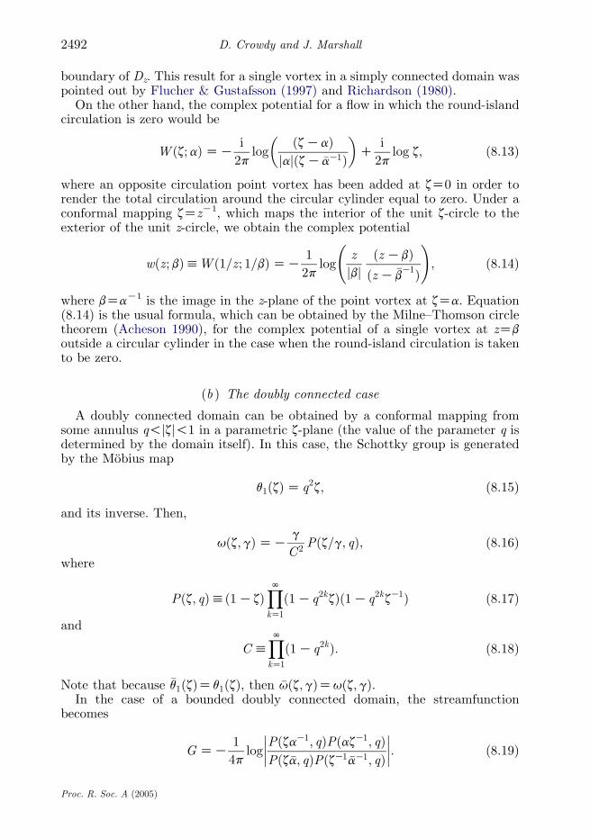
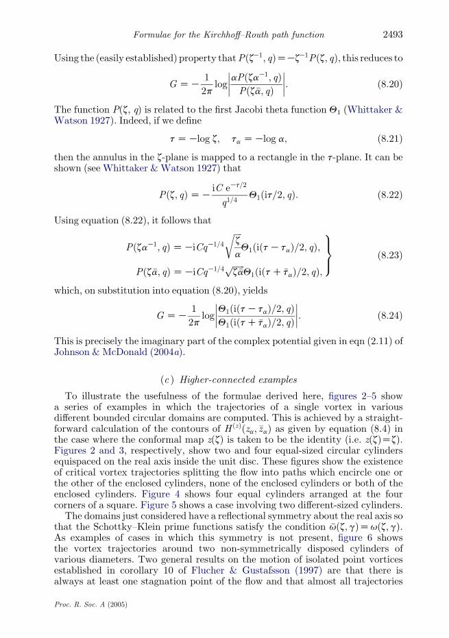
To illustrate the usefulness of the formulae derived here, figures 2–5 showa series of examples in which the trajectories of a single vortex in variousdifferent bounded circular domains are computed. This is achieved by a straight-forward calculation of the contours of H ðzÞðza; �zaÞ as given by equation (8.4) inthe case where the conformal map z(z) is taken to be the identity (i.e. z(z)Zz).Figures 2 and 3, respectively, show two and four equal-sized circular cylindersequispaced on the real axis inside the unit disc. These figures show the existenceof critical vortex trajectories splitting the flow into paths which encircle one orthe other of the enclosed cylinders, none of the enclosed cylinders or both of theenclosed cylinders. Figure 4 shows four equal cylinders arranged at the fourcorners of a square. Figure 5 shows a case involving two different-sized cylinders.

The domains just considered have a reflectional symmetry about the real axis sothat the Schottky–Klein prime functions satisfy the condition �uðz;gÞZuðz;gÞ.As examples of cases in which this symmetry is not present, figure 6 showsthe vortex trajectories around two non-symmetrically disposed cylinders ofvarious diameters. Two general results on the motion of isolated point vorticesestablished in corollary 10 of Flucher & Gustafsson (1997) are that there isalways at least one stagnation point of the flow and that almost all trajectories


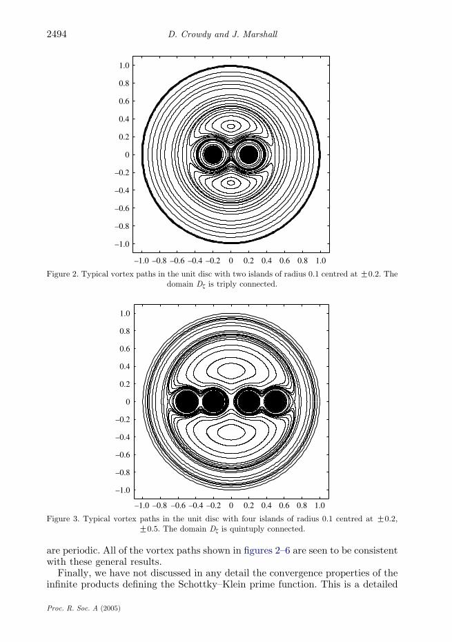
Figure 2. Typical vortex paths in the unit disc with two islands of radius 0.1 centred at G0.2. Thedomain Dz is triply connected.

Figure 3. Typical vortex paths in the unit disc with four islands of radius 0.1 centred at G0.2,G0.5. The domain Dz is quintuply connected.


are periodic. All of the vortex paths shown in figures 2–6 are seen to be consistentwith these general results.

Finally, we have not discussed in any detail the convergence properties of theinfinite products defining the Schottky–Klein prime function. This is a detailed


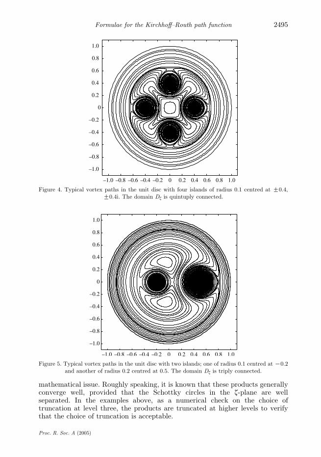
Figure 4. Typical vortex paths in the unit disc with four islands of radius 0.1 centred at G0.4,G0.4i. The domain Dz is quintuply connected.

Figure 5. Typical vortex paths in the unit disc with two islands; one of radius 0.1 centred at K0.2and another of radius 0.2 centred at 0.5. The domain Dz is triply connected.


mathematical issue. Roughly speaking, it is known that these products generallyconverge well, provided that the Schottky circles in the z-plane are wellseparated. In the examples above, as a numerical check on the choice oftruncation at level three, the products are truncated at higher levels to verifythat the choice of truncation is acceptable.


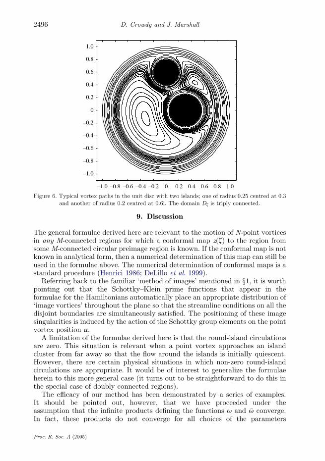
Figure 6. Typical vortex paths in the unit disc with two islands; one of radius 0.25 centred at 0.3and another of radius 0.2 centred at 0.6i. The domain Dz is triply connected.


9. Discussion

The general formulae derived here are relevant to the motion of N-point vorticesin any M-connected regions for which a conformal map z(z) to the region fromsome M-connected circular preimage region is known. If the conformal map is notknown in analytical form, then a numerical determination of this map can still beused in the formulae above. The numerical determination of conformal maps is astandard procedure (Henrici 1986; DeLillo et al. 1999).

Referring back to the familiar ‘method of images’ mentioned in §1, it is worthpointing out that the Schottky–Klein prime functions that appear in theformulae for the Hamiltonians automatically place an appropriate distribution of‘image vortices’ throughout the plane so that the streamline conditions on all thedisjoint boundaries are simultaneously satisfied. The positioning of these imagesingularities is induced by the action of the Schottky group elements on the pointvortex position a.

A limitation of the formulae derived here is that the round-island circulationsare zero. This situation is relevant when a point vortex approaches an islandcluster from far away so that the flow around the islands is initially quiescent.However, there are certain physical situations in which non-zero round-islandcirculations are appropriate. It would be of interest to generalize the formulaeherein to this more general case (it turns out to be straightforward to do this inthe special case of doubly connected regions).

The efficacy of our method has been demonstrated by a series of examples.It should be pointed out, however, that we have proceeded under theassumption that the infinite products defining the functions u and �u converge.In fact, these products do not converge for all choices of the parameters



fqj ; dj jjZ1;.;Mg. Broadly speaking, their convergence depends on thedistribution of circles fCj jjZ1;.;Mg in the preimage plane. If the circlesare ‘well-separated’, then good convergence is assured. There is a large regionof the parameter space fqj ; dj jjZ1;.;Mg where the convergence is completelyadequate for practical purposes. This region of parameter space is largeenough to capture many physically interesting fluid domains. Examples ofthese can be found in a companion article by the authors (Crowdy & Marshall2005), where the formulae of this paper have been combined with variouschoices of conformal maps to unbounded fluid domains of interest inapplications.

On the subject of applications, we conclude by mentioning a few. In arecent paper, Johnson & McDonald (2004a) consider the motion of a vortexin the doubly connected region exterior to two circular cylinders whoseboundaries act as impenetrable barriers for the flow. The motivation for thisstudy was to provide a simple model to understand how an oceanic eddy/vortexinteracts with topography (Simmons & Nof 2000). Such flow scenarios occur in arange of geophysical situations such as the interaction of Mediterranean saltlenses (‘Meddies’) with seamounts in the Canary basin (Dewar 2002) orthe collision of North Brazil current rings with the islands of the Caribbean(Simmons & Nof 2002). In their study, Johnson & McDonald (2004a) considerthe case in which the circulation around each island is zero, which is precisely thecase considered here. An important result of Johnson & McDonald (2004a) wasthat, in many cases, the motion of the centroid of a finite-area vortex patcharound topography is well-approximated by a point vortex model in the samedomain. Thus, one application of our results will be to provide useful checks onnumerical calculations of the motion of finite-area vortex patches aroundtopography. Other studies of geophysical interest involve the motion of vorticesnear gaps in an impenetrable barrier (Nof 1995; Johnson & McDonald 2004b,2005). The results here generalize the formulae of Johnson & McDonald (2004a)to any number of circular islands, and we expect our results to be of practical usein geophysical applications. Indeed, we have used the new formalism to study anumber of island configurations of geophysical interest, including islands off aninfinite coastline as well as island clusters in unbounded oceans (Crowdy &Marshall 2005).

J.M. acknowledges the support of an EPSRC studentship.

Appendix A. Proof of transformation property (5.9)

From the definition given in equations (5.1)–(5.3),

uðz;gÞZ ðzKgÞYqj2Q00

fz; qjðzÞ;g; qjðgÞg: (A 1)

By using equation (A 1),

uðzK1;gK1ÞZ ðzK1KgK1ÞYqj2Q00

fzK1; qjðzK1Þ;gK1; qjðgK1Þg: (A 2)



Consider a general term of the form qj(zK1). This is some composition of the

generators of the Schottky group. Suppose, for example, that

qjðzK1ÞZ qpðqqðqrðzK1ÞÞÞ; (A 3)

for some sequence of integers (p, q, r) labelling the level-one maps (such asequence of integers is sometimes called a ‘word’; Mumford et al. 2002). Recallfrom equation (4.6) that if qk is one of the basic level-one maps, then

qK1k ðzK1ÞZ 1

�qkðzÞ: (A 4)

Equivalently,

qkðzK1ÞZ 1

�qK1k ðzÞ

: (A 5)

By using equation (A5) repeatedly in equation (A 3),

qjðzK1ÞZ qpðqqðqrðzK1ÞÞÞZ qp qq1

�qK1r ðzÞ

! !Z qp

1

�qK1q ð�qK1

r ðzÞÞ

!

Z1

�qK1p ð�qK1

q ð�qK1r ðzÞÞÞ

Z1

qrqqqpK1ðzÞ

:

(A 6)

We now introduce a general subscript ‘r ’ notation; given the map qj (e.g.corresponding to the word (p, q, r)), then qjr will denote the map correspondingto the reversed word. In this example, the reversed word is (r, q, p) so that

qjr Z qrðqqðqpðzÞÞÞ: (A 7)

Then, equation (A 6) can be written

qjðzK1ÞZ 1

qjrK1ðzÞ

: (A 8)

It should be clear that the result in equation (A8) will be true for any map qj .It follows that

uðzK1;gK1ÞZðzK1 KgK1ÞYqj2Q00

1

z;

1

qjrK1ðzÞ

;1

g;

1

qjrK1ðgÞ

( )

ZðzK1 KgK1ÞYqj2Q00

z; qjrK1ðzÞ;g; qjr

K1ðgÞn o

;

(A 9)

where we have used the invariance of cross-ratios to Mobius transformation of allfour arguments. Now, using the fact that inverses are excluded from the product,



equation (A 9) can also be written

uðzK1;gK1ÞZ ðzK1 KgK1ÞYqj2Q00

fz; qjrðzÞ;g; qjrðgÞg; (A 10)

where we have simply relabelled the maps in the product. Furthermore, if amapping qj is included in the product, then it is easy to check that it can bearranged that the mapping qjr is also in the product. Thus, under a furtherrelabelling of the maps, equation (A10) becomes

uðzK1;gK1ÞZ ðzK1 KgK1ÞYqj2Q00

fz; qj ðzÞ;g; qj ðgÞg: (A 11)

Thus,

�uðzK1;gK1ÞZuð�zK1; �gK1Þ

ZðzK1 KgK1ÞYqj2Q00

fz; qjðzÞ;g; qjðgÞg

ZðzK1KgK1Þ uðz;gÞðzKgÞ

ZK1

zguðz;gÞ: (A 12)

This completes the proof. &

Appendix B. Proof that {bj(a; �aK1)} are real and positive

We now verify that the formula on the right-hand side of equation (6.14) gives areal positive quantity.

First, note that the product in equation (6.14) defining bjða; �aK1Þ is over mapsin the set Qj , which excludes those maps in Q with a power of qj or qK1

j on theright-hand end. Consider a typical term in the product, tkða; �aÞ say, associatedwith the map qk ,

tkða; �aÞZaKqkðBjÞaKqkðAjÞ

� ��aK1 KqkðAjÞ�aK1 KqkðBjÞ

� �: (B 1)

Its complex conjugate is

tkða; �aÞ Z�aK �qkð �BjÞ�aK �qkð �AjÞ

!aK1K �qkð �AjÞaK1K �qkð �BjÞ

!: (B 2)

However, from equation (A 8), it is known that for all mappings in the group

qK1k ðzK1ÞZ 1

�qkrðzÞ; (B 3)



which implies, in particular, that

�qkð �AjÞZ1

qK1kr ð �A

K1j Þ

; �qkð �BjÞZ1

qK1kr ð �B

K1j Þ

: (B 4)

By using these in equation (B 2) and after some rearrangement, we get

tkða; �aÞ ZaKqK1

kr ð �AK1j Þ

aKqK1kr ð �B

K1j Þ

!�aK1 KqK1

kr ð �BK1j Þ

�aK1 KqK1kr ð �A

K1j Þ

!: (B 5)

Now, observe that if Aj and Bj are the fixed points of qj (and hence also of qK1j ),

then �Aj , �Bj are necessarily the fixed points of �qj (and hence also of �qK1j ).

Substituting zZ �Aj ; �Bj in equation (B 3) yields

qK1j ð �AK1

j ÞZ �AK1j ; qK1

j ð �BK1j ÞZ �B

K1j ; (B 6)

from which we deduce the relations

Aj Z1�Bj

; Bj Z1�Aj

; (B 7)

where we have enforced the ordering jAjjOjBjj. By using equation (B 7) inequation (B 5), we deduce

tkða; �aÞ ZaKqK1

kr ðBjÞaKqK1

kr ðAjÞ

!�aK1 KqK1

kr ðAjÞ�aK1 KqK1

kr ðBjÞ

!: (B 8)

However, the right-hand side of equation (B 8) is precisely the term appearing inthe product associated with the map qK1

kr . It is straightforward to verify that if qkis in the set Qj , then so is the map qK1

kr . Thus, these two terms in the product aremutual complex conjugates and combine in pairs to give a positive real quantity.

qk and qK1kr are distinct except if qk is the identity. The outstanding term is

simply

ðaKBjÞð�aK1 KAjÞðaKAjÞð�aK1 KBjÞ

: (B 9)

Given that AjZBjK1

, this can be rewritten in the form

jAj j2aKBj

aKAj

��2; (B 10)

which is clearly real, and positive.In summary, the products defining the quantities fbjða; �aK1Þg are therefore

real and positive. &

References

Acheson, D. J. 1990 Elementary fluid dynamics. Oxford: Oxford University Press.Aref, H., Newton, P. K., Stremler, M., Tokieda, T. & Vainchtein, D. L. 2002 Vortex crystals. Adv.

Appl. Mech. 39.



Baker, H. 1995 Abelian functions. Cambridge: Cambridge University Press.Beardon, A. F. 1984 A primer on Riemann surfaces. In London Mathematical Society Lecture Notes

Series 78. Cambridge: Cambridge University Press.Crowdy, D. G. & Marshall, J. S. 2005 The motion of a point vortex around multiple circular

islands. Phys. Fluids. 17, 056602.DeLillo, T. K., Horn, M. A. & Pfaltzgraff, J. A. 1999 Numerical conformal mapping of multiply-

connected regions by Fornberg-like methods. Numerische Math. 83, 205–230.Dewar, W. K. 2002 Baroclinic eddy interaction with isolated topography. J. Phys. Oceanogr. 32,

2789–2805.Flucher, M. 1999 Variational problems with concentration. Basel: Birkhauser.Flucher, M. & Gustafsson, B. 1997 Vortex motion in two dimensional hydrodynamics TRITA-

MAT-1997-MA 02. Stockholm: Royal Institute of Technology.Gustafsson, B. 1979 On the motion of a vortex in two-dimensional flow of an ideal fluid in simply

and multiply connected domains TRITA-MAT-1979-7. Stockholm: Royal Institute ofTechnology.

Henrici, P. 1986 Applied and computational complex analysis. New York: Wiley Interscience.Johnson, E. R. & McDonald, N. R. 2004 The motion of a vortex near two circular cylinders. Proc.

R. Soc. A 460, 939–954. (doi:10.1098/rspa.2003.1193.)Johnson, E. R. & McDonald, N. R. 2004b The motion of a vortex near a gap in a wall. Phys. Fluids

16, 462–469.Johnson, E. R. & McDonald, N. R. 2005 Vortices near barriers with multiple gaps. J. Fluid Mech.

31, 355–358.Lin, C. C. 1941a On the motion of vortices in two dimensions. I. Existence of the Kirchhoff–Routh

function. Proc. Natl Acad. Sci. 27, 570–575.Lin, C. C. 1941b On the motion of vortices in two dimensions. II. Some further investigations on

the Kirchhoff–Routh function. Proc. Natl Acad. Sci. 27, 575–577.Milne-Thomson, L. M. 1968 Theoretical hydrodynamics. London: Macmillan.Mumford, D., Series, C. & Wright, D. 2002 Indra’s Pearls. Cambridge: Cambridge University

Press.Nehari, Z. 1952 Conformal mapping. New York: McGraw-Hill.Newton, P. K. 2002 The N-vortex problem. New York: Springer.Nof, D. 1995 Choked flows from the Pacific to the Indian Ocean. J. Phys. Oceanogr. 25, 1369.Richardson, S. 1980 Vortices, Liouville’s equation and the Bergman kernel function. Mathematika

27, 321–334.Routh, E. J. 1881 Some applications of conjugate functions. Proc. R. Soc. A 12, 73–89.Saffman, P. G. 1992 Vortex dynamics. Cambridge: Cambridge University Press.Simmons, H. L. & Nof, D. 2000 Islands as eddy splitters. J. Mar. Res. 58, 919–956.Simmons, H. L. & Nof, D. 2002 The squeezing of eddies through gaps. J. Phys. Oceanogr. 32, 314.Whittaker, E. T. & Watson, G. N. 1927 A course of modern analysis. Cambridge: Cambridge

University Press.

As this paper exceeds the maximum length normally permitted,the authors have agreed to contribute to production costs.


http://dx.doi.org/doi:10.1098/rspa.2003.1193

analytical formulae for the kirchhoff–routh path function in multiply...

Documents