appendices dr susan walker evidence kidd mcintyre appeals

Appendices to evidence-in-chief of Susan Walker, 27 October 2017 page 1

APPENDICES to the evidence-in-chief of Susan Walker, 27 October 2017

APPENDIX Numbered page

Appendix 1. Copy of access Agreement: Simons Pass And Simons Hill 2

Appendix 2. Major landform and climate gradients in the Mackenzie Basin 6

Appendix 3. Ecological components of the natural landscape character of the Mackenzie

Basin subzone 12

Appendix 4. Ecologically important climatic features of the Mackenzie Basin floor 12

Appendix 5. The New Zealand Threat Classification System 21

Appendix 6. Photographs of transport of materials on wind in comparable environments 23

Appendix 7. Brochure “Surface Inversions For Australian Agricultural Regions” 25


Appendix 1. Copy of access agreement: Simons Pass and Simons Hill


Appendix 2. Major landform and climate gradients in the Mackenzie Basin Map A2.1 Simplified glacial geomorphology of the Mackenzie Basin floor, derived from Barrell et al. (2011).

Moraines

Outwash gravels

Application sites

Ecological districtboundaries

Mackenzie districtboundary

Highways

25 km


Map A2.2 Detailed glacial geomorphology of the Mackenzie Basin floor, derived from Barrell et al. (2012).

Source: Barrell DJA, Andersen BG, Denton GH 2011. Glacial geomorphology of the central South Island, New Zealand. GNS Science monograph 27. Lower Hutt, GNS Science.

Late Otiranoutwash surface

Holocene alluvial plain or terrace

Latest late Otiranoutwash surface

4.0 km


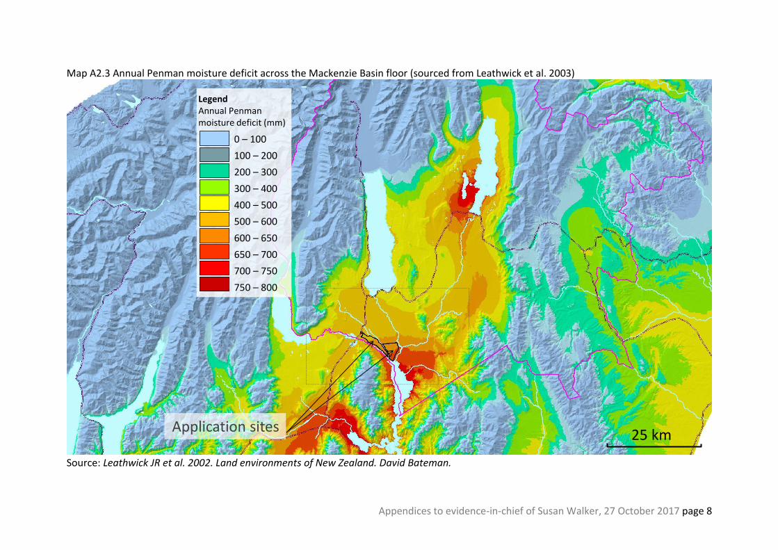
Map A2.3 Annual Penman moisture deficit across the Mackenzie Basin floor (sourced from Leathwick et al. 2003)

Source: Leathwick JR et al. 2002. Land environments of New Zealand. David Bateman.

LegendAnnual Penman moisture deficit (mm)

0 – 100

100 – 200

200 – 300

300 – 400

400 – 500

500 – 600

600 – 650

650 – 700

700 – 750

750 – 800

Application sites25 km


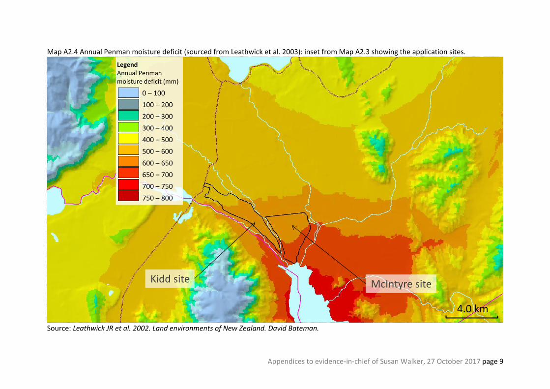
Map A2.4 Annual Penman moisture deficit (sourced from Leathwick et al. 2003): inset from Map A2.3 showing the application sites.


LegendAnnual Penman moisture deficit (mm)

0 – 100

100 – 200

200 – 300

300 – 400

400 – 500

500 – 600

600 – 650

650 – 700

700 – 750

750 – 800

Kidd site McIntyre site

4.0 km


Map A2.5 October vapour pressure deficit across the Mackenzie Basin floor (sourced from Leathwick et al. 2003)


LegendOctober vapourpressure deficit(kPa)

0 – 40

40 – 42

42 – 44

44 – 46

46 – 48

48 – 50

Application sites25 km


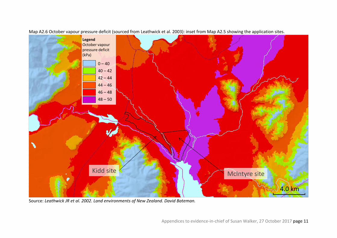
Map A2.6 October vapour pressure deficit (sourced from Leathwick et al. 2003): inset from Map A2.5 showing the application sites.


LegendOctober vapourpressure deficit(kPa)

0 – 40

40 – 42

42 – 44

44 – 46

46 – 48

48 – 50

Kidd site McIntyre site

4.0 km


Appendix 3.

Ecological components of the natural landscape character of the Mackenzie Basin subzone

‘Ecosystems’ including historically rare ecosystems based on geomorphological features NOTE: Parentheses indicate the land types of Lynn (1993) and Environment Canterbury (2010) within which these ecosystems are mainly (bold type) or more occasionally found. Lake margins and deltas (H3) Connected sequences of moraines of different ages (H3) Striated moraines framing lakes (H3) Terminal moraines (H3) Rugged and hummocky young moraines (H3, H4) Subdued older rolling moraine surfaces (usually further from lakes) (H3, H4) Erratic boulders and boulderfields (H3, H4) Kettlehole tarns and ephemeral wetlands (H3, H4) Seepages and flushes (H3, H4) Ephemeral streams (H3, H4) Other wetland types and systems on and within depositional surfaces (H3, H4) Outwash gravel terraces and fans (H3, H4) Braided dry meltwater outwash channels (H3, H4) Inland sand dunes (H1) Terraces separating different depositional surfaces (H3, H4) Series of terraces (H3, H4) Braided rivers and associated alluvial surfaces (H3, H4) Rivers, streams and associated alluvium issuing from surrounding ranges (H3, H4, H17) Ice-sculpted hills within basin (H7) Footslopes of ranges and hills (H3, H4, H7) Alluvial and colluvial fans (H3, H4, H7) Gradients, sequences, patterns, ecotones and transitions Wet north-west to drier south-east aridity gradient Sequences of different soils across the aridity gradient Sequences of moraines of different ages Moist western moraines with tall and short tussock grassland Drier moraines with short tussock grassland and herbfields Moraines cut by outwash and meltwater channels of different ages Extensive, continuous, undeveloped moraine-outwash-alluvium sequences Complexes of outwash and alluvial gravel surfaces of different ages Transitions or ecotones between different depositional (glacial and alluvial) landforms Series and flights of terraces (high and/or low, and different ages) Terrace brows, scarps, and toes Micro-habitat and soil variation (including aspect-related) within moraines Ridge and hollow micro-topography on outwash gravels


Ecological components of the natural landscape character of the Mackenzie Basin subzone (continued) Vegetation and flora Extensive and little-fragmented sequences of vegetation Tall and short tussock grasslands and their native inter-tussock flora Matagouri shubland and wild spaniard Ephemeral wetlands and their turfs Lakeshore and delta plant communities Wetlands, wetland complexes, and their vegetation Alternation of sparse and better-vegetated surfaces on outwash gravels and alluvium Braided vegetation patterns on outwash and alluvium Grey and mixed shrublands and their native flora Mat and cushion vegetation, including hawkweed-dominated Mossfields, lichenfields, and non-vascular crusts Exposed stonefields Prostrate or low-growing native flora Spring annual and seasonal geophytes (orchids, ferns) and their habitats Non-vascular species (including lichens, mosses, and fungi) in all habitats Xerophytic (drought-adapted) endemic flora At risk and threatened flora Fauna (including habitats) Native and endemic wading birds, terns and gulls of braided rivers, outwash surfaces and moraine wetlands Extensive seasonal breeding habitats of banded dotterel and pied oystercatcher, especially sparsely-vegetated outwash and alluvial surfaces Native wetland bird fauna Grey shrubland native bird fauna New Zealand pipit and their mixed grassland habitats (especially moraine) Endemic lizards and their habitats including mixed grasslands, erratics and bouldery surfaces Endemic insect species characteristic of different habitats Endemic freshwater fish fauna of clear unpolluted streams Xerophytic (drought-adapted) endemic fauna At risk and threatened fauna REFERENCES Environment Canterbury 2010. Canterbury Regional Landscape Study Review – Final Report – July 2010. http://ecan.govt.nz/publications/Plans/canterbury-regional-landscape-study-review-2010.pdf Lynn IH 1993. Land types of the Canterbury Region. Landcare Research New Zealand and Lucas Associates.


Appendix 4. Ecologically important climatic features of the Mackenzie Basin floor

The data shown in this Appendix were derived from the national climate database CLiFlo maintained by NIWA (https://cliflo.niwa.co.nz/). Figure A4.1. Daily temperature ranges, daily maximum temperature, and daily minimum temperature in each of the twelve calendar months (denoted by their first letter) over the last 10 years at Pukaki Aerodrome (upper row, 44.23⁰S, 170.11⁰E, 473m a.s.l.) and the last ~9 years at Tara Hills (lower row, 44.53⁰S, 168.89⁰E, 488 m a.s.l.). These are the two nearest climate stations to the application sites with temperature records. The figures are box and whisker plots, in which the horizontal black lines are the median value, the boxes show the interquartile range (i.e. the middle 50% of values), and the whiskers extend to the extreme maximum and minimum values. The figures shows that large daily temperature ranges are regularly experienced in the Mackenzie Basin, especially in summer, when night time temperatures generally fall to <10⁰C, and that frosts can be experienced in any month.

https://cliflo.niwa.co.nz/


Figure A4.2. Day and night wind roses for Lake Tekapo (44.00⁰S, 170.44⁰E, 780m a.s.l., the nearest meteorological site with wind records) between 1 October and 31 March over the years 2003 to 2016. The bars show the frequency (in %) of counts aggregated by the direction from which the wind is coming, and average wind speed, in the 10 minute period preceding each hour. Widths of the coloured bars indicate the percentage of time that winds are experienced from one of the eight principal wind directions: north (‘N’) 338 to 22⁰, northeast 23 to 67⁰, east (‘E’) 68 to 112⁰, southeast 113 to 157⁰, south (‘S’) 158 to 202⁰, southwest 203 to 247⁰, west (‘W’) 248 to 292⁰, and northwest (293 to 337⁰) within a wind speed band (0 to 2, 2 to 4, 4 to 6, or 6 to 25 metres per second). The figures show that strong northerly and northwesterly winds predominate during the day in the summer growing season, and that there are generally lighter winds at night, which that are dominated by gentle northerly katabatic breezes.

Day (9am to 8pm) Night (9pm to 8am)

W

S

N

E

5%

10%

15%

20%

25%

30%

35%

40%

45%

50%

0 to 2 2 to 4 4 to 6 6 to 24.9

metres per second

W

S

N

E

5%

10%

15%

20%

25%

30%

35%

40%

45%

50%

0 to 2 2 to 4 4 to 6 6 to 24.9

metres per second

0 to 2 2 to 4 4 to 6 6 to 25Average wind speed over the 10 minute

period preceding each hour, in metres per second


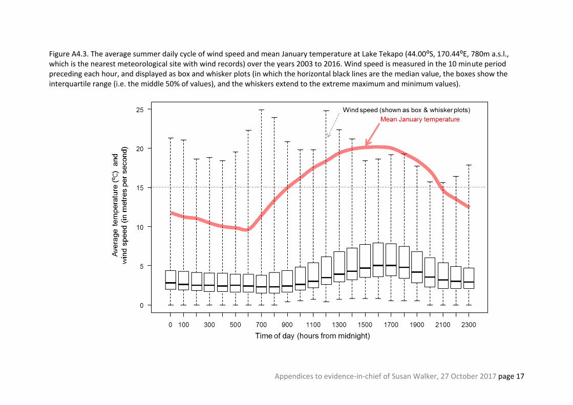
Figure A4.3. The average summer daily cycle of wind speed and mean January temperature at Lake Tekapo (44.00⁰S, 170.44⁰E, 780m a.s.l., which is the nearest meteorological site with wind records) over the years 2003 to 2016. Wind speed is measured in the 10 minute period preceding each hour, and displayed as box and whisker plots (in which the horizontal black lines are the median value, the boxes show the interquartile range (i.e. the middle 50% of values), and the whiskers extend to the extreme maximum and minimum values).


Figure A4.4. Relative humidity in calendar months at the Tara Hills/Omarama climate station between 1951 and 2017, presented as box and whisker plots which show the medians (solid lines), interquartile ranges (boxes), and extremes (upper and lower whiskers). Note that the climate station name was changed to Omarama when measurement technology changed in 1985, but the location (44.53⁰S, 168.89⁰E, 488 m a.s.l.) remained the same. As can be seen in C., humidity has changed little between the periods before and after 1985.


Figure A4.5. The difference between the 9am air temperature and the dew point in calendar months at the at the Tara Hills/Omarama climate station between 1972 and 2017. The box and whisker plots show the medians (solid lines), interquartile ranges (boxes), and extremes (upper and lower whiskers). Note that the climate station name was changed to Omarama when measurement technology changed in 1985, but the location (44.53⁰S, 168.89⁰E, 488 m a.s.l.) remained the same. Values greater than zero mean that the air temperature is higher than the dew point temperature, so that moisture in the air will not condense.


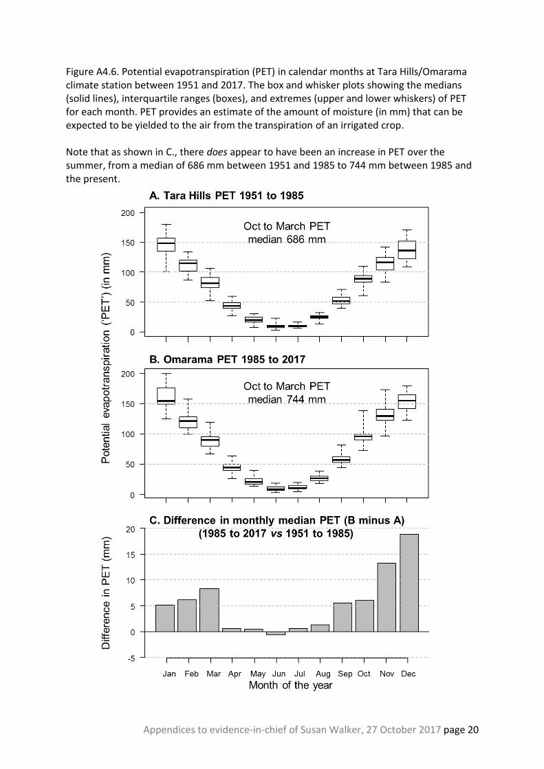
Figure A4.6. Potential evapotranspiration (PET) in calendar months at Tara Hills/Omarama climate station between 1951 and 2017. The box and whisker plots showing the medians (solid lines), interquartile ranges (boxes), and extremes (upper and lower whiskers) of PET for each month. PET provides an estimate of the amount of moisture (in mm) that can be expected to be yielded to the air from the transpiration of an irrigated crop. Note that as shown in C., there does appear to have been an increase in PET over the summer, from a median of 686 mm between 1951 and 1985 to 744 mm between 1985 and the present.


Appendix 5. The New Zealand Threat Classification System

In New Zealand, candidate taxa in different biotic groups (e.g. vascular plants, birds, bats, lizards, fungi) are evaluated and placed in different categories of risk according to the criteria outlined by Townsend et al. (2008) and shown in the Figure below.

Evaluated taxa are placed in one of the following categories:

• Extinct (those for which there is now no reasonable doubt – following repeated surveys in known or expected habitats at appropriate times (diurnal, seasonal and annual) and throughout the plant’s historic range – that the last individual has died);

• Threatened (with three subcategories – Nationally Critical, Nationally Endangered, and Nationally Vulnerable – which represent a sequence of decreasing extinction risk);

• At Risk (with four subcategories – Declining, Recovering, Relict, and Naturally Uncommon – of which Declining species are considered to be at greatest risk);

• Not Threatened (the category of lowest risk).

Townsend AJ, de Lange PJ, Norton DA, Molloy J, Miskelly C, Duffy C 2008. The New Zealand Threat Classification System manual. Wellington, Department of Conservation. 30 p.


Threatened and at risk taxa are defined as follows:

Threatened

Nationally Critical taxa, which are “Nationally Critical A”– very small population (natural or unnatural); “Nationally Critical B”– small population (natural or unnatural) with a high ongoing or predicted decline; or “Nationally Critical C”– population (irrespective of size or number of sub-populations) with a very high ongoing or predicted decline (>70%).

Nationally Endangered taxa, which are “Nationally Endangered A”– small population (natural or unnatural) that has a low to high ongoing or predicted decline; “Nationally Endangered B”– small stable population (unnatural); or “Nationally Endangered C”– moderate population and high ongoing or predicted decline.

Nationally Vulnerable taxa, which are “Nationally Vulnerable A”– small, increasing population (unnatural); “Nationally Vulnerable B”– moderate, stable population (unnatural); “Nationally Vulnerable C”– moderate population, with population trend that is declining; “Nationally Vulnerable D”– moderate to large population and moderate to high ongoing or predicted decline; or “Nationally Vulnerable D”– large population and high ongoing or predicted decline.

At Risk

Declining taxa include “Declining A”– moderate to large population and low ongoing or predicted decline; “Declining B”– large population and low to moderate ongoing or predicted decline; and “Declining C”– very large population and low to high ongoing or predicted decline.

Naturally Uncommon taxa are those whose distribution is naturally confined to specific substrates (e.g. ultramafic rock), habitats (e.g. high alpine fellfield, hydrothermal vents), or geographic areas (e.g. subantarctic islands, seamounts), or taxa that occur within naturally small and widely scattered populations. This distribution is not the result of past or recent human disturbance. Populations may be stable or increasing. Note that a naturally uncommon taxon that has <250 mature individuals qualifies for Nationally Critical. Taxa that have >20,000 mature individuals are not considered Naturally Uncommon, unless they occupy an area of <100,000 ha (1000 km2).

Data Deficient taxa are suspected to belong to one of the above categories, but this is not definitely known due to a lack of current information about their present-day distribution and abundance. It is hoped that listing such taxa will stimulate research to find out the true category of threat.


Appendix 6. Photographs of transport of materials on wind in comparable environments


Appendix 7. Brochure “Surface Inversions for Australian Agricultural Regions”

This brochure is distributed by the Cotton Field Awareness Map, an Australian industry initiative which has been designed to highlight the location of cotton fields. The service is provided free of charge with the purpose of minimising off-target damage from downwind pesticide application, particularly during fallow spraying. (http://www.cottonmap.com.au/Content/documents/Temperature%20Inversions.pdf)

http://www.cottonmap.com.au/Content/documents/Temperature%20Inversions.pdf

appendices dr susan walker evidence kidd mcintyre appeals

Documents